Linear Algebra
Linear Algebra
Linear Algebra

You also want an ePaper? Increase the reach of your titles
YUMPU automatically turns print PDFs into web optimized ePapers that Google loves.
� �<br />
�<br />
�1<br />
2�<br />
�<br />
�3 1�<br />
<strong>Linear</strong> <strong>Algebra</strong><br />
� �<br />
�<br />
�x<br />
· 1 2�<br />
�<br />
�x · 3 1�<br />
Jim Hefferon<br />
� �<br />
�<br />
�6<br />
2�<br />
�<br />
�8 1�
Notation<br />
R real numbers<br />
N natural numbers: {0, 1, 2,...}<br />
C complex numbers<br />
{... � � ...} set of ... such that ...<br />
〈...〉 sequence; like a set but order matters<br />
V,W,U vector spaces<br />
�v, �w vectors<br />
�0, �0V zero vector, zero vector of V<br />
B,D bases<br />
En = 〈�e1, ... , �en〉 standard basis for R n<br />
�β, � δ basis vectors<br />
Rep B(�v) matrix representing the vector<br />
Pn set of n-th degree polynomials<br />
Mn×m set of n×m matrices<br />
[S] span of the set S<br />
M ⊕ N direct sum of subspaces<br />
V ∼ = W isomorphic spaces<br />
h, g homomorphisms<br />
H, G matrices<br />
t, s transformations; maps from a space to itself<br />
T,S square matrices<br />
Rep B,D(h) matrix representing the map h<br />
hi,j matrix entry from row i, column j<br />
|T | determinant of the matrix T<br />
R(h), N (h) rangespace and nullspace of the map h<br />
R∞(h), N∞(h) generalized rangespace and nullspace<br />
Lower case Greek alphabet<br />
name symbol name symbol name symbol<br />
alpha α iota ι rho ρ<br />
beta β kappa κ sigma σ<br />
gamma γ lambda λ tau τ<br />
delta δ mu µ upsilon υ<br />
epsilon ɛ nu ν phi φ<br />
zeta ζ xi ξ chi χ<br />
eta η omicron o psi ψ<br />
theta θ pi π omega ω<br />
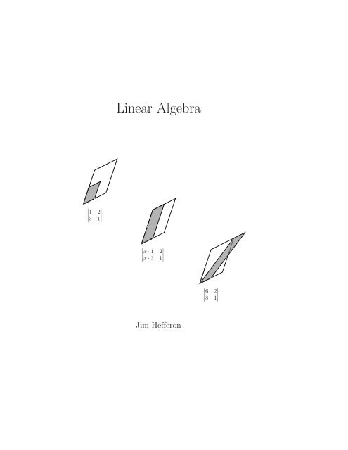
Cover. This is Cramer’s Rule applied to the system x +2y =6,3x + y =8. Thearea<br />
of the first box is the determinant shown. The area of the second box is x times that,<br />
and equals the area of the final box. Hence, x is the final determinant divided by the<br />
first determinant.
Preface<br />
In most mathematics programs linear algebra is taken in the first or second<br />
year, following or along with at least one course in calculus. While the location<br />
of this course is stable, lately the content has been under discussion. Some instructors<br />
have experimented with varying the traditional topics, trying courses<br />
focused on applications, or on the computer. Despite this (entirely healthy)<br />
debate, most instructors are still convinced, I think, that the right core material<br />
is vector spaces, linear maps, determinants, and eigenvalues and eigenvectors.<br />
Applications and computations certainly can have a part to play but most mathematicians<br />
agree that the themes of the course should remain unchanged.<br />
Not that all is fine with the traditional course. Most of us do think that<br />
the standard text type for this course needs to be reexamined. Elementary<br />
texts have traditionally started with extensive computations of linear reduction,<br />
matrix multiplication, and determinants. These take up half of the course.<br />
Finally, when vector spaces and linear maps appear, and definitions and proofs<br />
start, the nature of the course takes a sudden turn. In the past, the computation<br />
drill was there because, as future practitioners, students needed to be fast and<br />
accurate with these. But that has changed. Being a whiz at 5×5 determinants<br />
just isn’t important anymore. Instead, the availability of computers gives us an<br />
opportunity to move toward a focus on concepts.<br />
This is an opportunity that we should seize. The courses at the start of<br />
most mathematics programs work at having students correctly apply formulas<br />
and algorithms, and imitate examples. Later courses require some mathematical<br />
maturity: reasoning skills that are developed enough to follow different types<br />
of proofs, a familiarity with the themes that underly many mathematical investigations<br />
like elementary set and function facts, and an ability to do some<br />
independent reading and thinking, Where do we work on the transition?<br />
<strong>Linear</strong> algebra is an ideal spot. It comes early in a program so that progress<br />
made here pays off later. The material is straightforward, elegant, and accessible.<br />
The students are serious about mathematics, often majors and minors.<br />
There are a variety of argument styles—proofs by contradiction, if and only if<br />
statements, and proofs by induction, for instance—and examples are plentiful.<br />
The goal of this text is, along with the development of undergraduate linear<br />
algebra, to help an instructor raise the students’ level of mathematical sophistication.<br />
Most of the differences between this book and others follow straight<br />
from that goal.<br />
One consequence of this goal of development is that, unlike in many computational<br />
texts, all of the results here are proved. On the other hand, in contrast<br />
with more abstract texts, many examples are given, and they are often quite<br />
detailed.<br />
Another consequence of the goal is that while we start with a computational<br />
topic, linear reduction, from the first we do more than just compute. The<br />
solution of linear systems is done quickly but it is also done completely, proving<br />
i
everything (really these proofs are just verifications), all the way through the<br />
uniqueness of reduced echelon form. In particular, in this first chapter, the<br />
opportunity is taken to present a few induction proofs, where the arguments<br />
just go over bookkeeping details, so that when induction is needed later (e.g., to<br />
prove that all bases of a finite dimensional vector space have the same number<br />
of members), it will be familiar.<br />
Still another consequence is that the second chapter immediately uses this<br />
background as motivation for the definition of a real vector space. This typically<br />
occurs by the end of the third week. We do not stop to introduce matrix<br />
multiplication and determinants as rote computations. Instead, those topics<br />
appear naturally in the development, after the definition of linear maps.<br />
To help students make the transition from earlier courses, the presentation<br />
here stresses motivation and naturalness. An example is the third chapter,<br />
on linear maps. It does not start with the definition of homomorphism, as<br />
is the case in other books, but with the definition of isomorphism. That’s<br />
because this definition is easily motivated by the observation that some spaces<br />
are just like each other. After that, the next section takes the reasonable step of<br />
defining homomorphisms by isolating the operation-preservation idea. A little<br />
mathematical slickness is lost, but it is in return for a large gain in sensibility<br />
to students.<br />
Having extensive motivation in the text helps with time pressures. I ask<br />
students to, before each class, look ahead in the book, and they follow the<br />
classwork better because they have some prior exposure to the material. For<br />
example, I can start the linear independence class with the definition because I<br />
know students have some idea of what it is about. No book can take the place<br />
of an instructor, but a helpful book gives the instructor more class time for<br />
examples and questions.<br />
Much of a student’s progress takes place while doing the exercises; the exercises<br />
here work with the rest of the text. Besides computations, there are many<br />
proofs. These are spread over an approachability range, from simple checks<br />
to some much more involved arguments. There are even a few exercises that<br />
are reasonably challenging puzzles taken, with citation, from various journals,<br />
competitions, or problems collections (as part of the fun of these, the original<br />
wording has been retained as much as possible). In total, the questions are<br />
aimed to both build an ability at, and help students experience the pleasure of,<br />
doing mathematics.<br />
Applications, and Computers. The point of view taken here, that linear<br />
algebra is about vector spaces and linear maps, is not taken to the exclusion<br />
of all other ideas. Applications, and the emerging role of the computer, are<br />
interesting, important, and vital aspects of the subject. Consequently, every<br />
chapter closes with a few application or computer-related topics. Some of the<br />
topics are: network flows, the speed and accuracy of computer linear reductions,<br />
Leontief Input/Output analysis, dimensional analysis, Markov chains, voting<br />
paradoxes, analytic projective geometry, and solving difference equations.<br />
These are brief enough to be done in a day’s class or to be given as indepen-<br />
ii
dent projects for individuals or small groups. Most simply give a reader a feel<br />
for the subject, discuss how linear algebra comes in, point to some accessible<br />
further reading, and give a few exercises. I have kept the exposition lively and<br />
given an overall sense of breadth of application. In short, these topics invite<br />
readers to see for themselves that linear algebra is a tool that a professional<br />
must have.<br />
For people reading this book on their own. The emphasis on motivation<br />
and development make this book a good choice for self-study. While a professional<br />
mathematician knows what pace and topics suit a class, perhaps an<br />
independent student would find some advice helpful. Here are two timetables<br />
for a semester. The first focuses on core material.<br />
week Mon. Wed. Fri.<br />
1 1.I.1 1.I.1, 2 1.I.2, 3<br />
2 1.I.3 1.II.1 1.II.2<br />
3 1.III.1, 2 1.III.2 2.I.1<br />
4 2.I.2 2.II 2.III.1<br />
5 2.III.1, 2 2.III.2 exam<br />
6 2.III.2, 3 2.III.3 3.I.1<br />
7 3.I.2 3.II.1 3.II.2<br />
8 3.II.2 3.II.2 3.III.1<br />
9 3.III.1 3.III.2 3.IV.1, 2<br />
10 3.IV.2, 3, 4 3.IV.4 exam<br />
11 3.IV.4, 3.V.1 3.V.1, 2 4.I.1, 2<br />
12 4.I.3 4.II 4.II<br />
13 4.III.1 5.I 5.II.1<br />
14 5.II.2 5.II.3 review<br />
The second timetable is more ambitious (it presupposes 1.II, the elements of<br />
vectors, usually covered in third semester calculus).<br />
week Mon. Wed. Fri.<br />
1 1.I.1 1.I.2 1.I.3<br />
2 1.I.3 1.III.1, 2 1.III.2<br />
3 2.I.1 2.I.2 2.II<br />
4 2.III.1 2.III.2 2.III.3<br />
5 2.III.4 3.I.1 exam<br />
6 3.I.2 3.II.1 3.II.2<br />
7 3.III.1 3.III.2 3.IV.1, 2<br />
8 3.IV.2 3.IV.3 3.IV.4<br />
9 3.V.1 3.V.2 3.VI.1<br />
10 3.VI.2 4.I.1 exam<br />
11 4.I.2 4.I.3 4.I.4<br />
12 4.II 4.II, 4.III.1 4.III.2, 3<br />
13 5.II.1, 2 5.II.3 5.III.1<br />
14 5.III.2 5.IV.1, 2 5.IV.2<br />
See the table of contents for the titles of these subsections.<br />
iii
For guidance, in the table of contents I have marked some subsections as<br />
optional if, in my opinion, some instructors will pass over them in favor of<br />
spending more time elsewhere. These subsections can be dropped or added, as<br />
desired. You might also adjust the length of your study by picking one or two<br />
Topics that appeal to you from the end of each chapter. You’ll probably get<br />
more out of these if you have access to computer software that can do the big<br />
calculations.<br />
Do many exercises. (The answers are available.) I have marked a good sample<br />
with �’s. Be warned about the exercises, however, that few inexperienced<br />
people can write correct proofs. Try to find a knowledgeable person to work<br />
with you on this aspect of the material.<br />
Finally, if I may, a caution: I cannot overemphasize how much the statement<br />
(which I sometimes hear), “I understand the material, but it’s only that I can’t<br />
do any of the problems.” reveals a lack of understanding of what we are up<br />
to. Being able to do particular things with the ideas is the entire point. The<br />
quote below expresses this sentiment admirably, and captures the essence of<br />
this book’s approach. It states what I believe is the key to both the beauty and<br />
the power of mathematics and the sciences in general, and of linear algebra in<br />
particular.<br />
I know of no better tactic<br />
than the illustration of exciting principles<br />
by well-chosen particulars.<br />
–Stephen Jay Gould<br />
Jim Hefferon<br />
Saint Michael’s College<br />
Colchester, Vermont USA<br />
jim@joshua.smcvt.edu<br />
April 20, 2000<br />
Author’s Note. Inventing a good exercise, one that enlightens as well as tests,<br />
is a creative act, and hard work (at least half of the the effort on this text<br />
has gone into exercises and solutions). The inventor deserves recognition. But,<br />
somehow, the tradition in texts has been to not give attributions for questions.<br />
I have changed that here where I was sure of the source. I would greatly appreciate<br />
hearing from anyone who can help me to correctly attribute others of the<br />
questions. They will be incorporated into later versions of this book.<br />
iv
Contents<br />
1 <strong>Linear</strong> Systems 1<br />
1.I Solving <strong>Linear</strong> Systems ........................ 1<br />
1.I.1 Gauss’ Method ........................... 2<br />
1.I.2 Describing the Solution Set .................... 11<br />
1.I.3 General = Particular + Homogeneous .............. 20<br />
1.II <strong>Linear</strong> Geometry of n-Space ...................... 32<br />
1.II.1 Vectors in Space .......................... 32<br />
1.II.2 Length and Angle Measures ∗ ................... 38<br />
1.III Reduced Echelon Form ........................ 45<br />
1.III.1 Gauss-Jordan Reduction ...................... 45<br />
1.III.2 Row Equivalence .......................... 51<br />
Topic: Computer <strong>Algebra</strong> Systems ..................... 61<br />
Topic: Input-Output Analysis ....................... 63<br />
Topic: Accuracy of Computations ..................... 67<br />
Topic: Analyzing Networks ......................... 72<br />
2 Vector Spaces 79<br />
2.I Definition of Vector Space ....................... 80<br />
2.I.1 Definition and Examples ...................... 80<br />
2.I.2 Subspaces and Spanning Sets ................... 91<br />
2.II <strong>Linear</strong> Independence ..........................102<br />
2.II.1 Definition and Examples ......................102<br />
2.III Basis and Dimension ..........................113<br />
2.III.1 Basis .................................113<br />
2.III.2 Dimension ..............................119<br />
2.III.3 Vector Spaces and <strong>Linear</strong> Systems ................124<br />
2.III.4 Combining Subspaces ∗ .......................131<br />
Topic: Fields .................................141<br />
Topic: Crystals ................................143<br />
Topic: Voting Paradoxes ..........................147<br />
Topic: Dimensional Analysis ........................152<br />
v
3 Maps Between Spaces 159<br />
3.I Isomorphisms ..............................159<br />
3.I.1 Definition and Examples ......................159<br />
3.I.2 Dimension Characterizes Isomorphism ..............169<br />
3.II Homomorphisms ............................176<br />
3.II.1 Definition ..............................176<br />
3.II.2 Rangespace and Nullspace .....................184<br />
3.III Computing <strong>Linear</strong> Maps ........................194<br />
3.III.1 Representing <strong>Linear</strong> Maps with Matrices ............194<br />
3.III.2 Any Matrix Represents a <strong>Linear</strong> Map ∗ ..............204<br />
3.IV Matrix Operations ...........................211<br />
3.IV.1 Sums and Scalar Products .....................211<br />
3.IV.2 Matrix Multiplication .......................214<br />
3.IV.3 Mechanics of Matrix Multiplication ................221<br />
3.IV.4 Inverses ...............................230<br />
3.V Change of Basis ............................238<br />
3.V.1 Changing Representations of Vectors ...............238<br />
3.V.2 Changing Map Representations ..................242<br />
3.VI Projection ................................250<br />
3.VI.1 Orthogonal Projection Into a Line ∗ ................250<br />
3.VI.2 Gram-Schmidt Orthogonalization ∗ ................255<br />
3.VI.3 Projection Into a Subspace ∗ ....................260<br />
Topic: Line of Best Fit ...........................269<br />
Topic: Geometry of <strong>Linear</strong> Maps ......................274<br />
Topic: Markov Chains ............................280<br />
Topic: Orthonormal Matrices ........................286<br />
4 Determinants 293<br />
4.I Definition ................................294<br />
4.I.1 Exploration ∗ ............................294<br />
4.I.2 Properties of Determinants ....................299<br />
4.I.3 The Permutation Expansion ....................303<br />
4.I.4 Determinants Exist ∗ ........................312<br />
4.II Geometry of Determinants ......................319<br />
4.II.1 Determinants as Size Functions ..................319<br />
4.III Other Formulas .............................326<br />
4.III.1 Laplace’s Expansion ∗ .......................326<br />
Topic: Cramer’s Rule ............................331<br />
Topic: Speed of Calculating Determinants .................334<br />
Topic: Projective Geometry .........................337<br />
5 Similarity 347<br />
5.I Complex Vector Spaces ........................347<br />
5.I.1 Factoring and Complex Numbers; A Review ∗ ..........348<br />
5.I.2 Complex Representations .....................350<br />
5.II Similarity ................................351<br />
vi
5.II.1 Definition and Examples ......................351<br />
5.II.2 Diagonalizability ..........................353<br />
5.II.3 Eigenvalues and Eigenvectors ...................357<br />
5.III Nilpotence ...............................365<br />
5.III.1 Self-Composition ∗ .........................365<br />
5.III.2 Strings ∗ ...............................368<br />
5.IV Jordan Form ..............................379<br />
5.IV.1 Polynomials of Maps and Matrices ∗ ...............379<br />
5.IV.2 Jordan Canonical Form ∗ ......................386<br />
Topic: Computing Eigenvalues—the Method of Powers .........399<br />
Topic: Stable Populations ..........................403<br />
Topic: <strong>Linear</strong> Recurrences .........................405<br />
Appendix A-1<br />
Introduction .................................A-1<br />
Propositions .................................A-1<br />
Quantifiers .................................A-3<br />
Techniques of Proof ............................A-5<br />
Sets, Functions, and Relations .......................A-6<br />
∗ Note: starred subsections are optional.<br />
vii
Chapter 1<br />
<strong>Linear</strong> Systems<br />
1.I Solving <strong>Linear</strong> Systems<br />
Systems of linear equations are common in science and mathematics. These two<br />
examples from high school science [Onan] give a sense of how they arise.<br />
The first example is from Physics. Suppose that we are given three objects,<br />
one with a mass of 2 kg, and are asked to find the unknown masses. Suppose<br />
further that experimentation with a meter stick produces these two balances.<br />
h<br />
40 50<br />
c<br />
15<br />
2<br />
c<br />
25 50<br />
Now, since the sum of moments on the left of each balance equals the sum of<br />
moments on the right (the moment of an object is its mass times its distance<br />
from the balance point), the two balances give this system of two equations.<br />
40h +15c = 100<br />
25c =50+50h<br />
The second example of a linear system is from Chemistry. We can mix,<br />
under controlled conditions, toluene C7H8 and nitric acid HNO3 to produce<br />
trinitrotoluene C7H5O6N3 along with the byproduct water (conditions have to<br />
be controlled very well, indeed — trinitrotoluene is better known as TNT). In<br />
what proportion should those components be mixed? The number of atoms of<br />
each element present before the reaction<br />
x C7H8 + y HNO3 −→ z C7H5O6N3 + w H2O<br />
must equal the number present afterward. Applying that principle to the elements<br />
C, H, N, and O in turn gives this system.<br />
7x =7z<br />
8x +1y =5z +2w<br />
1y =3z<br />
3y =6z +1w<br />
1<br />
25<br />
2<br />
h
2 Chapter 1. <strong>Linear</strong> Systems<br />
To finish each of these examples requires solving a system of equations. In<br />
each, the equations involve only the first power of the variables. This chapter<br />
shows how to solve any such system.<br />
1.I.1 Gauss’ Method<br />
1.1 Definition A linear equation in variables x1,x2,... ,xn has the form<br />
a1x1 + a2x2 + a3x3 + ···+ anxn = d<br />
where the numbers a1,... ,an ∈ R are the equation’s coefficients and d ∈ R is<br />
the constant. Ann-tuple (s1,s2,... ,sn) ∈ R n is a solution of, or satisfies, that<br />
equation if substituting the numbers s1, ... , sn for the variables gives a true<br />
statement: a1s1 + a2s2 + ...+ ansn = d.<br />
A system of linear equations<br />
a1,1x1 + a1,2x2 + ···+ a1,nxn = d1<br />
a2,1x1 + a2,2x2 + ···+ a2,nxn = d2<br />
.<br />
am,1x1 + am,2x2 + ···+ am,nxn = dm<br />
has the solution (s1,s2,... ,sn) if that n-tuple is a solution of all of the equations<br />
in the system.<br />
1.2 Example The ordered pair (−1, 5) is a solution of this system.<br />
In contrast, (5, −1) is not a solution.<br />
3x1 +2x2 =7<br />
−x1 + x2 =6<br />
Finding the set of all solutions is solving the system. No guesswork or good<br />
fortune is needed to solve a linear system. There is an algorithm that always<br />
works. The next example introduces that algorithm, called Gauss’ method. It<br />
transforms the system, step by step, into one with a form that is easily solved.<br />
1.3 Example To solve this system<br />
3x3 =9<br />
x1 +5x2 − 2x3 =2<br />
1<br />
3 x1 +2x2<br />
=3
Section I. Solving <strong>Linear</strong> Systems 3<br />
we repeatedly transform it until it is in a form that is easy to solve.<br />
swap row 1 with row 3<br />
−→<br />
multiply row 1 by 3<br />
−→<br />
add −1 times row 1 to row 2<br />
−→<br />
1<br />
3x1 +2x2<br />
=3<br />
x1 +5x2 − 2x3 =2<br />
3x3 =9<br />
x1 +6x2 =9<br />
x1 +5x2 − 2x3 =2<br />
3x3 =9<br />
x1 + 6x2 = 9<br />
−x2 − 2x3 = −7<br />
3x3 = 9<br />
The third step is the only nontrivial one. We’ve mentally multiplied both sides<br />
of the first row by −1, mentally added that to the old second row, and written<br />
the result in as the new second row.<br />
Now we can find the value of each variable. The bottom equation shows<br />
that x3 = 3. Substituting 3 for x3 in the middle equation shows that x2 =1.<br />
Substituting those two into the top equation gives that x1 = 3 and so the system<br />
has a unique solution: the solution set is { (3, 1, 3) }.<br />
Most of this subsection and the next one consists of examples of solving<br />
linear systems by Gauss’ method. We will use it throughout this book. It is<br />
fast and easy. But, before we get to those examples, we will first show that<br />
this method is also safe in that it never loses solutions or picks up extraneous<br />
solutions.<br />
1.4 Theorem (Gauss’ method) If a linear system is changed to another by<br />
one of these operations<br />
(1) an equation is swapped with another<br />
(2) an equation has both sides multiplied by a nonzero constant<br />
(3) an equation is replaced by the sum of itself and a multiple of another<br />
then the two systems have the same set of solutions.<br />
Each of those three operations has a restriction. Multiplying a row by 0 is<br />
not allowed because obviously that can change the solution set of the system.<br />
Similarly, adding a multiple of a row to itself is not allowed because adding −1<br />
times the row to itself has the effect of multiplying the row by 0. Finally, swapping<br />
a row with itself is disallowed to make some results in the fourth chapter<br />
easier to state and remember (and besides, self-swapping doesn’t accomplish<br />
anything).<br />
Proof. We will cover the equation swap operation here and save the other two<br />
cases for Exercise 29.
4 Chapter 1. <strong>Linear</strong> Systems<br />
Consider this swap of row i with row j.<br />
a1,1x1 + a1,2x2 + ··· a1,nxn = d1 a1,1x1 + a1,2x2 + ··· a1,nxn = d1<br />
.<br />
.<br />
.<br />
.<br />
ai,1x1 + ai,2x2 + ··· ai,nxn = di aj,1x1 + aj,2x2 + ··· aj,nxn = dj<br />
. −→<br />
.<br />
aj,1x1 + aj,2x2 + ··· aj,nxn = dj ai,1x1 + ai,2x2 + ··· ai,nxn = di<br />
.<br />
.<br />
.<br />
.<br />
am,1x1 + am,2x2 + ··· am,nxn = dm am,1x1 + am,2x2 + ··· am,nxn = dm<br />
The n-tuple (s1,... ,sn) satisfies the system before the swap if and only if<br />
substituting the values, the s’s, for the variables, the x’s, gives true statements:<br />
a1,1s1+a1,2s2+···+a1,nsn = d1 and ... ai,1s1+ai,2s2+···+ai,nsn = di and ...<br />
aj,1s1 + aj,2s2 + ···+ aj,nsn = dj and ... am,1s1 + am,2s2 + ···+ am,nsn = dm.<br />
In a requirement consisting of statements and-ed together we can rearrange<br />
the order of the statements, so that this requirement is met if and only if a1,1s1+<br />
a1,2s2 + ···+ a1,nsn = d1 and ... aj,1s1 + aj,2s2 + ···+ aj,nsn = dj and ...<br />
ai,1s1 + ai,2s2 + ···+ ai,nsn = di and ... am,1s1 + am,2s2 + ···+ am,nsn = dm.<br />
This is exactly the requirement that (s1,... ,sn) solves the system after the row<br />
swap. QED<br />
1.5 Definition The three operations from Theorem 1.4 are the elementary reduction<br />
operations, orrow operations, orGaussian operations. They are swapping,<br />
multiplying by a scalar or rescaling, andpivoting.<br />
When writing out the calculations, we will abbreviate ‘row i’ by‘ρi’. For<br />
instance, we will denote a pivot operation by kρi + ρj, with the row that is<br />
changed written second. We will also, to save writing, often list pivot steps<br />
together when they use the same ρi.<br />
1.6 Example A typical use of Gauss’ method is to solve this system.<br />
x + y =0<br />
2x − y +3z =3<br />
x − 2y − z =3<br />
The first transformation of the system involves using the first row to eliminate<br />
the x in the second row and the x in the third. To get rid of the second row’s<br />
2x, we multiply the entire first row by −2, add that to the second row, and<br />
write the result in as the new second row. To get rid of the third row’s x, we<br />
multiply the first row by −1, add that to the third row, and write the result in<br />
as the new third row.<br />
−ρ1+ρ3<br />
−→<br />
−2ρ1+ρ2<br />
x + y =0<br />
−3y +3z =3<br />
−3y − z =3<br />
(Note that the two ρ1 steps −2ρ1 + ρ2 and −ρ1 + ρ3 are written as one operation.)<br />
In this second system, the last two equations involve only two unknowns.
Section I. Solving <strong>Linear</strong> Systems 5<br />
To finish we transform the second system into a third system, where the last<br />
equation involves only one unknown. This transformation uses the second row<br />
to eliminate y from the third row.<br />
−ρ2+ρ3<br />
−→<br />
x + y =0<br />
−3y + 3z =3<br />
−4z =0<br />
Now we are set up for the solution. The third row shows that z = 0. Substitute<br />
that back into the second row to get y = −1, and then substitute back into the<br />
firstrowtogetx =1.<br />
1.7 Example For the Physics problem from the start of this chapter, Gauss’<br />
method gives this.<br />
40h +15c = 100<br />
−50h +25c = 50<br />
5/4ρ1+ρ2<br />
−→<br />
40h + 15c = 100<br />
(175/4)c = 175<br />
So c = 4, and back-substitution gives that h = 1. (The Chemistry problem is<br />
solved later.)<br />
1.8 Example The reduction<br />
x + y + z =9<br />
2x +4y − 3z =1<br />
3x +6y − 5z =0<br />
shows that z =3,y = −1, and x =7.<br />
−2ρ1+ρ2<br />
−→<br />
−3ρ1+ρ3<br />
−(3/2)ρ2+ρ3<br />
−→<br />
x + y + z = 9<br />
2y − 5z = −17<br />
3y − 8z = −27<br />
x + y + z = 9<br />
2y − 5z = −17<br />
− 1 3<br />
2z = − 2<br />
As these examples illustrate, Gauss’ method uses the elementary reduction<br />
operations to set up back-substitution.<br />
1.9 Definition In each row, the first variable with a nonzero coefficient is the<br />
row’s leading variable. A system is in echelon form if each leading variable is<br />
to the right of the leading variable in the row above it (except for the leading<br />
variable in the first row).<br />
1.10 Example The only operation needed in the examples above is pivoting.<br />
Here is a linear system that requires the operation of swapping equations. After<br />
the first pivot<br />
x − y =0<br />
2x − 2y + z +2w =4<br />
y + w =0<br />
2z + w =5<br />
−2ρ1+ρ2<br />
−→<br />
x − y =0<br />
z +2w =4<br />
y + w =0<br />
2z + w =5
6 Chapter 1. <strong>Linear</strong> Systems<br />
the second equation has no leading y. To get one, we look lower down in the<br />
system for a row that has a leading y and swap it in.<br />
ρ2↔ρ3<br />
−→<br />
x − y =0<br />
y + w =0<br />
z +2w =4<br />
2z + w =5<br />
(Had there been more than one row below the second with a leading y then we<br />
could have swapped in any one.) The rest of Gauss’ method goes as before.<br />
−2ρ3+ρ4<br />
−→<br />
x − y = 0<br />
y + w = 0<br />
z + 2w = 4<br />
−3w = −3<br />
Back-substitution gives w =1,z =2,y = −1, and x = −1.<br />
Strictly speaking, the operation of rescaling rows is not needed to solve linear<br />
systems. We have included it because we will use it later in this chapter as part<br />
of a variation on Gauss’ method, the Gauss-Jordan method.<br />
All of the systems seen so far have the same number of equations as unknowns.<br />
All of them have a solution, and for all of them there is only one<br />
solution. We finish this subsection by seeing for contrast some other things that<br />
can happen.<br />
1.11 Example <strong>Linear</strong> systems need not have the same number of equations<br />
as unknowns. This system<br />
x +3y = 1<br />
2x + y = −3<br />
2x +2y = −2<br />
has more equations than variables. Gauss’ method helps us understand this<br />
system also, since this<br />
−2ρ1+ρ2<br />
−→<br />
−2ρ1+ρ3<br />
x + 3y = 1<br />
−5y = −5<br />
−4y = −4<br />
shows that one of the equations is redundant. Echelon form<br />
−(4/5)ρ2+ρ3<br />
−→<br />
x + 3y = 1<br />
−5y = −5<br />
0= 0<br />
gives y =1andx = −2. The ‘0 = 0’ is derived from the redundancy.
Section I. Solving <strong>Linear</strong> Systems 7<br />
That example’s system has more equations than variables. Gauss’ method<br />
is also useful on systems with more variables than equations. Many examples<br />
are in the next subsection.<br />
Another way that linear systems can differ from the examples shown earlier<br />
is that some linear systems do not have a unique solution. This can happen in<br />
two ways.<br />
The first is that it can fail to have any solution at all.<br />
1.12 Example Contrast the system in the last example with this one.<br />
x +3y = 1<br />
2x + y = −3<br />
2x +2y = 0<br />
−2ρ1+ρ2<br />
−→<br />
−2ρ1+ρ3<br />
x + 3y = 1<br />
−5y = −5<br />
−4y = −2<br />
Here the system is inconsistent: no pair of numbers satisfies all of the equations<br />
simultaneously. Echelon form makes this inconsistency obvious.<br />
The solution set is empty.<br />
−(4/5)ρ2+ρ3<br />
−→<br />
x + 3y = 1<br />
−5y = −5<br />
0= 2<br />
1.13 Example The prior system has more equations than unknowns, but that<br />
is not what causes the inconsistency — Example 1.11 has more equations than<br />
unknowns and yet is consistent. Nor is having more equations than unknowns<br />
necessary for inconsistency, as is illustrated by this inconsistent system with the<br />
same number of equations as unknowns.<br />
x +2y =8<br />
2x +4y =8<br />
−2ρ1+ρ2<br />
−→<br />
x +2y = 8<br />
0=−8<br />
The other way that a linear system can fail to have a unique solution is to<br />
have many solutions.<br />
1.14 Example In this system<br />
x + y =4<br />
2x +2y =8<br />
any pair of numbers satisfying the first equation automatically satisfies the second.<br />
The solution set {(x, y) � � x + y =4} is infinite — some of its members<br />
are (0, 4), (−1, 5), and (2.5, 1.5). The result of applying Gauss’ method here<br />
contrasts with the prior example because we do not get a contradictory equation.<br />
−2ρ1+ρ2<br />
−→<br />
x + y =4<br />
0=0
8 Chapter 1. <strong>Linear</strong> Systems<br />
Don’t be fooled by the ‘0 = 0’ equation in that example. It is not the signal<br />
that a system has many solutions.<br />
1.15 Example The absence of a ‘0 = 0’ does not keep a system from having<br />
many different solutions. This system is in echelon form<br />
x + y + z =0<br />
y + z =0<br />
has no ‘0 = 0’, and yet has infinitely many solutions. (For instance, each of<br />
these is a solution: (0, 1, −1), (0, 1/2, −1/2), (0, 0, 0), and (0, −π, π). There are<br />
infinitely many solutions because any triple whose first component is 0 and<br />
whose second component is the negative of the third is a solution.)<br />
Nor does the presence of a ‘0 = 0’ mean that the system must have many<br />
solutions. Example 1.11 shows that. So does this system, which does not have<br />
many solutions — in fact it has none — despite that when it is brought to<br />
echelon form it has a ‘0 = 0’ row.<br />
2x − 2z =6<br />
y + z =1<br />
2x + y − z =7<br />
3y +3z =0<br />
−ρ1+ρ3<br />
−→<br />
−ρ2+ρ3<br />
−→<br />
−3ρ2+ρ4<br />
2x − 2z =6<br />
y + z =1<br />
y + z =1<br />
3y +3z =0<br />
2x − 2z = 6<br />
y + z = 1<br />
0= 0<br />
0=−3<br />
We will finish this subsection with a summary of what we’ve seen so far<br />
about Gauss’ method.<br />
Gauss’ method uses the three row operations to set a system up for back<br />
substitution. If any step shows a contradictory equation then we can stop<br />
with the conclusion that the system has no solutions. If we reach echelon form<br />
without a contradictory equation, and each variable is a leading variable in its<br />
row, then the system has a unique solution and we find it by back substitution.<br />
Finally, if we reach echelon form without a contradictory equation, and there is<br />
not a unique solution (at least one variable is not a leading variable) then the<br />
system has many solutions.<br />
The next subsection deals with the third case — we will see how to describe<br />
the solution set of a system with many solutions.<br />
Exercises<br />
� 1.16 Use Gauss’ method to find the unique solution for each system.<br />
x − z =0<br />
2x +3y = 13<br />
(a) (b) 3x + y =1<br />
x − y = −1<br />
−x + y + z =4<br />
� 1.17 Use Gauss’ method to solve each system or conclude ‘many solutions’ or ‘no<br />
solutions’.
Section I. Solving <strong>Linear</strong> Systems 9<br />
(a) 2x +2y =5 (b) −x + y =1 (c) x − 3y + z = 1<br />
x − 4y =0 x + y =2 x + y +2z =14<br />
(d) −x − y =1 (e) 4y + z =20 (f) 2x + z + w = 5<br />
−3x − 3y =2 2x − 2y + z = 0<br />
y − w = −1<br />
x + z = 5 3x − z − w = 0<br />
x + y − z =10 4x + y +2z + w = 9<br />
� 1.18 There are methods for solving linear systems other than Gauss’ method. One<br />
often taught in high school is to solve one of the equations for a variable, then<br />
substitute the resulting expression into other equations. That step is repeated<br />
until there is an equation with only one variable. From that, the first number in<br />
the solution is derived, and then back-substitution can be done. This method both<br />
takes longer than Gauss’ method, since it involves more arithmetic operations and<br />
is more likely to lead to errors. To illustrate how it can lead to wrong conclusions,<br />
we will use the system<br />
x +3y = 1<br />
2x + y = −3<br />
2x +2y = 0<br />
from Example 1.12.<br />
(a) Solve the first equation for x and substitute that expression into the second<br />
equation. Find the resulting y.<br />
(b) Again solve the first equation for x, but this time substitute that expression<br />
into the third equation. Find this y.<br />
What extra step must a user of this method take to avoid erroneously concluding<br />
a system has a solution?<br />
� 1.19 For which values of k are there no solutions, many solutions, or a unique<br />
solution to this system?<br />
x − y =1<br />
3x − 3y = k<br />
� 1.20 This system is not linear:<br />
2sinα− cos β +3tanγ = 3<br />
4sinα +2cosβ−2tanγ =10<br />
6sinα− 3cosβ + tanγ = 9<br />
but we can nonetheless apply Gauss’ method.<br />
solution?<br />
Do so. Does the system have a<br />
� 1.21 What conditions must the constants, the b’s, satisfy so that each of these<br />
systems has a solution? Hint. Apply Gauss’ method and see what happens to the<br />
right side.<br />
(a) x − 3y = b1 (b) x1 +2x2 +3x3 = b1<br />
3x + y = b2 2x1 +5x2 +3x3 = b2<br />
x +7y = b3<br />
2x +4y = b4<br />
x1 +8x3 = b3<br />
1.22 True or false: a system with more unknowns than equations has at least one<br />
solution. (As always, to say ‘true’ you must prove it, while to say ‘false’ you must<br />
produce a counterexample.)<br />
1.23 Must any Chemistry problem like the one that starts this subsection — a<br />
balance the reaction problem — have infinitely many solutions?<br />
� 1.24 Find the coefficients a, b, andcso that the graph of f(x) =ax 2 +bx+c passes<br />
through the points (1, 2), (−1, 6), and (2, 3).
10 Chapter 1. <strong>Linear</strong> Systems<br />
1.25 Gauss’ method works by combining the equations in a system to make new<br />
equations.<br />
(a) Can the equation 3x−2y = 5 be derived, by a sequence of Gaussian reduction<br />
steps, from the equations in this system?<br />
x + y =1<br />
4x − y =6<br />
(b) Can the equation 5x−3y = 2 be derived, by a sequence of Gaussian reduction<br />
steps, from the equations in this system?<br />
2x +2y =5<br />
3x + y =4<br />
(c) Can the equation 6x − 9y +5z = −2 be derived, by a sequence of Gaussian<br />
reduction steps, from the equations in the system?<br />
2x + y − z =4<br />
6x − 3y + z =5<br />
1.26 Prove that, where a,b,... ,e are real numbers and a �= 0,if<br />
ax + by = c<br />
has the same solution set as<br />
ax + dy = e<br />
then they are the same equation. What if a =0?<br />
� 1.27 Show that if ad − bc �= 0then<br />
ax + by = j<br />
cx + dy = k<br />
has a unique solution.<br />
� 1.28 In the system<br />
ax + by = c<br />
dx + ey = f<br />
each of the equations describes a line in the xy-plane. By geometrical reasoning,<br />
show that there are three possibilities: there is a unique solution, there is no<br />
solution, and there are infinitely many solutions.<br />
1.29 Finish the proof of Theorem 1.4.<br />
1.30 Is there a two-unknowns linear system whose solution set is all of R 2 ?<br />
� 1.31 Are any of the operations used in Gauss’ method redundant? That is, can<br />
any of the operations be synthesized from the others?<br />
1.32 Prove that each operation of Gauss’ method is reversible. That is, show that if<br />
two systems are related by a row operation S1 ↔ S2 then there is a row operation<br />
to go back S2 ↔ S1.<br />
1.33 A box holding pennies, nickels and dimes contains thirteen coins with a total<br />
value of 83 cents. How many coins of each type are in the box?<br />
1.34 [Con. Prob. 1955] Four positive integers are given. Select any three of the<br />
integers, find their arithmetic average, and add this result to the fourth integer.<br />
Thus the numbers 29, 23, 21, and 17 are obtained. One of the original integers<br />
is:
Section I. Solving <strong>Linear</strong> Systems 11<br />
(a) 19 (b) 21 (c) 23 (d) 29 (e) 17<br />
� 1.35 [Am. Math. Mon., Jan. 1935] Laugh at this: AHAHA + TEHE = TEHAW.<br />
It resulted from substituting a code letter for each digit of a simple example in<br />
addition, and it is required to identify the letters and prove the solution unique.<br />
1.36 [Wohascum no. 2] The Wohascum County Board of Commissioners, which has<br />
20 members, recently had to elect a President. There were three candidates (A, B,<br />
and C); on each ballot the three candidates were to be listed in order of preference,<br />
with no abstentions. It was found that 11 members, a majority, preferred A over<br />
B (thus the other 9 preferred B over A). Similarly, it was found that 12 members<br />
preferred C over A. Given these results, it was suggested that B should withdraw,<br />
to enable a runoff election between A and C. However, B protested, and it was<br />
then found that 14 members preferred B over C! The Board has not yet recovered<br />
from the resulting confusion. Given that every possible order of A, B, C appeared<br />
on at least one ballot, how many members voted for B as their first choice?<br />
1.37 [Am. Math. Mon., Jan. 1963] “This system of n linear equations with n unknowns,”<br />
said the Great Mathematician, “has a curious property.”<br />
“Good heavens!” said the Poor Nut, “What is it?”<br />
“Note,” said the Great Mathematician, “that the constants are in arithmetic<br />
progression.”<br />
“It’s all so clear when you explain it!” said the Poor Nut. “Do you mean like<br />
6x +9y =12and15x +18y = 21?”<br />
“Quite so,” said the Great Mathematician, pulling out his bassoon. “Indeed,<br />
the system has a unique solution. Can you find it?”<br />
“Good heavens!” cried the Poor Nut, “I am baffled.”<br />
Are you?<br />
1.I.2 Describing the Solution Set<br />
A linear system with a unique solution has a solution set with one element.<br />
A linear system with no solution has a solution set that is empty. In these cases<br />
the solution set is easy to describe. Solution sets are a challenge to describe<br />
only when they contain many elements.<br />
2.1 Example This system has many solutions because in echelon form<br />
2x + z =3<br />
x − y − z =1<br />
3x − y =4<br />
−(1/2)ρ1+ρ2<br />
−→<br />
−(3/2)ρ1+ρ3<br />
−ρ2+ρ3<br />
−→<br />
2x + z = 3<br />
−y − (3/2)z = −1/2<br />
−y − (3/2)z = −1/2<br />
2x + z = 3<br />
−y − (3/2)z = −1/2<br />
0= 0<br />
not all of the variables are leading variables. The Gauss’ method theorem<br />
showed that a triple satisfies the first system if and only if it satisfies the third.<br />
Thus, the solution set {(x, y, z) � � 2x + z =3andx − y − z =1and3x − y =4}
12 Chapter 1. <strong>Linear</strong> Systems<br />
can also be described as {(x, y, z) � � 2x + z =3and−y − 3z/2 =−1/2}. However,<br />
this second description is not much of an improvement. It has two equations<br />
instead of three, but it still involves some hard-to-understand interaction<br />
among the variables.<br />
To get a description that is free of any such interaction, we take the variable<br />
that does not lead any equation, z, and use it to describe the variables<br />
that do lead, x and y. The second equation gives y = (1/2) − (3/2)z and<br />
the first equation gives x =(3/2) − (1/2)z. Thus, the solution set can be described<br />
as {(x, y, z) = ((3/2) − (1/2)z,(1/2) − (3/2)z,z) � � z ∈ R}. For instance,<br />
(1/2, −5/2, 2) is a solution because taking z = 2 gives a first component of 1/2<br />
and a second component of −5/2.<br />
The advantage of this description over the ones above is that the only variable<br />
appearing, z, is unrestricted — it can be any real number.<br />
2.2 Definition The non-leading variables in an echelon-form linear system are<br />
free variables.<br />
In the echelon form system derived in the above example, x and y are leading<br />
variables and z is free.<br />
2.3 Example A linear system can end with more than one variable free. This<br />
row reduction<br />
x + y + z − w = 1<br />
y − z + w = −1<br />
3x +6z − 6w = 6<br />
−y + z − w = 1<br />
−3ρ1+ρ3<br />
−→<br />
3ρ2+ρ3<br />
−→<br />
ρ2+ρ4<br />
x + y + z − w = 1<br />
y − z + w = −1<br />
−3y +3z − 3w = 3<br />
−y + z − w = 1<br />
x + y + z − w = 1<br />
y − z + w = −1<br />
0= 0<br />
0= 0<br />
ends with x and y leading, and with both z and w free. To get the description<br />
that we prefer we will start at the bottom. We first express y in terms of<br />
the free variables z and w with y = −1 +z − w. Next, moving up to the<br />
top equation, substituting for y in the first equation x +(−1 +z − w) +z −<br />
w = 1 and solving for x yields x =2− 2z +2w. Thus, the solution set is<br />
{2 − 2z +2w, −1+z − w, z, w) � � z,w ∈ R}.<br />
We prefer this description because the only variables that appear, z and w,<br />
are unrestricted. This makes the job of deciding which four-tuples are system<br />
solutions into an easy one. For instance, taking z =1andw = 2 gives the<br />
solution (4, −2, 1, 2). In contrast, (3, −2, 1, 2) is not a solution, since the first<br />
component of any solution must be 2 minus twice the third component plus<br />
twice the fourth.
Section I. Solving <strong>Linear</strong> Systems 13<br />
2.4 Example After this reduction<br />
2x − 2y =0<br />
z +3w =2<br />
3x − 3y =0<br />
x − y +2z +6w =4<br />
−(3/2)ρ1+ρ3<br />
−→<br />
−(1/2)ρ1+ρ4<br />
−2ρ2+ρ4<br />
−→<br />
2x − 2y =0<br />
z +3w =2<br />
0=0<br />
2z +6w =4<br />
2x − 2y =0<br />
z +3w =2<br />
0=0<br />
0=0<br />
x and z lead, y and w are free. The solution set is {(y, y, 2 − 3w, w) � � y, w ∈ R}.<br />
For instance, (1, 1, 2, 0) satisfies the system — take y =1andw =0. The<br />
four-tuple (1, 0, 5, 4) is not a solution since its first coordinate does not equal its<br />
second.<br />
We refer to a variable used to describe a family of solutions as a parameter<br />
and we say that the set above is paramatrized with y and w. (The terms<br />
‘parameter’ and ‘free variable’ do not mean the same thing. Above, y and w<br />
are free because in the echelon form system they do not lead any row. They<br />
are parameters because they are used in the solution set description. We could<br />
have instead paramatrized with y and z by rewriting the second equation as<br />
w =2/3− (1/3)z. In that case, the free variables are still y and w, but the<br />
parameters are y and z. Notice that we could not have paramatrized with x and<br />
y, so there is sometimes a restriction on the choice of parameters. The terms<br />
‘parameter’ and ‘free’ are related because, as we shall show later in this chapter,<br />
the solution set of a system can always be paramatrized with the free variables.<br />
Consequenlty, we shall paramatrize all of our descriptions in this way.)<br />
2.5 Example This is another system with infinitely many solutions.<br />
x +2y =1<br />
2x + z =2<br />
3x +2y + z − w =4<br />
−2ρ1+ρ2<br />
−→<br />
−3ρ1+ρ3<br />
−ρ2+ρ3<br />
−→<br />
x + 2y =1<br />
−4y + z =0<br />
−4y + z − w =1<br />
x + 2y =1<br />
−4y + z =0<br />
−w =1<br />
The leading variables are x, y, andw. The variable z is free. (Notice here that,<br />
although there are infinitely many solutions, the value of one of the variables is<br />
fixed — w = −1.) Write w in terms of z with w = −1+0z. Then y =(1/4)z.<br />
To express x in terms of z, substitute for y into the first equation to get x =<br />
1 − (1/2)z. The solution set is {(1 − (1/2)z,(1/4)z,z,−1) � � z ∈ R}.<br />
We finish this subsection by developing the notation for linear systems and<br />
their solution sets that we shall use in the rest of this book.<br />
2.6 Definition An m×n matrix is a rectangular array of numbers with m rows<br />
and n columns. Each number in the matrix is an entry,
14 Chapter 1. <strong>Linear</strong> Systems<br />
Matrices are usually named by upper case roman letters, e.g. A. Each entry is<br />
denoted by the corresponding lower-case letter, e.g. ai,j is the number in row i<br />
and column j of the array. For instance,<br />
A =<br />
�<br />
1 2.2<br />
�<br />
5<br />
3 4 −7<br />
has two rows and three columns, and so is a 2×3 matrix. (Read that “twoby-three”;<br />
the number of rows is always stated first.) The entry in the second<br />
row and first column is a2,1 = 3. Note that the order of the subscripts matters:<br />
a1,2 �= a2,1 since a1,2 =2.2. (The parentheses around the array are a typographic<br />
device so that when two matrices are side by side we can tell where one<br />
ends and the other starts.)<br />
2.7 Example We can abbreviate this linear system<br />
with this matrix.<br />
x1 +2x2 =4<br />
x2 − x3 =0<br />
+2x3 =4<br />
x1<br />
⎛<br />
1<br />
⎝0<br />
2<br />
1<br />
0<br />
−1<br />
⎞<br />
4<br />
0⎠<br />
1 0 2 4<br />
The vertical bar just reminds a reader of the difference between the coefficients<br />
on the systems’s left hand side and the constants on the right. When a bar<br />
is used to divide a matrix into parts, we call it an augmented matrix. In this<br />
notation, Gauss’ method goes this way.<br />
⎛<br />
⎞<br />
1 2 0 4<br />
⎝0<br />
1 −1 0⎠<br />
1 0 2 4<br />
−ρ1+ρ3<br />
⎛<br />
⎞<br />
1 2 0 4<br />
−→ ⎝0<br />
1 −1 0⎠<br />
0 −2 2 0<br />
2ρ2+ρ3<br />
⎛<br />
⎞<br />
1 2 0 4<br />
−→ ⎝0<br />
1 −1 0⎠<br />
0 0 0 0<br />
The second row stands for y − z = 0 and the first row stands for x +2y =4so<br />
the solution set is {(4 − 2z,z,z) � � z ∈ R}. One advantage of the new notation is<br />
that the clerical load of Gauss’ method — the copying of variables, the writing<br />
of +’s and =’s, etc. — is lighter.<br />
We will also use the array notation to clarify the descriptions of solution<br />
sets. A description like {(2 − 2z +2w, −1+z − w, z, w) � � z,w ∈ R} from Example<br />
2.3 is hard to read. We will rewrite it to group all the constants together,<br />
all the coefficients of z together, and all the coefficients of w together. We will<br />
write them vertically, in one-column wide matrices.<br />
⎛ ⎞<br />
2<br />
⎜<br />
{ ⎜−1<br />
⎟<br />
⎝ 0 ⎠<br />
0<br />
+<br />
⎛ ⎞ ⎛ ⎞<br />
−2 2<br />
⎜ 1 ⎟ ⎜<br />
⎟<br />
⎝ 1 ⎠ · z + ⎜−1<br />
⎟<br />
⎝ 0 ⎠<br />
0 1<br />
· w � � z,w ∈ R}
Section I. Solving <strong>Linear</strong> Systems 15<br />
For instance, the top line says that x =2− 2z +2w. The next section gives a<br />
geometric interpretation that will help us picture the solution sets when they<br />
are written in this way.<br />
2.8 Definition A vector (or column vector) is a matrix with a single column.<br />
A matrix with a single row is a row vector. The entries of a vector are its<br />
components.<br />
Vectors are an exception to the convention of representing matrices with<br />
capital roman letters. We use lower-case roman or greek letters overlined with<br />
an arrow: �a, �b, ... or �α, � β, ... (boldface is also common: a or α). For<br />
instance, this is a column vector with a third component of 7.<br />
⎛<br />
�v = ⎝ 1<br />
⎞<br />
3⎠<br />
7<br />
2.9 Definition The linear equation a1x1 + a2x2 + ··· + anxn = d with unknowns<br />
x1,... ,xn is satisfied by<br />
⎛ ⎞<br />
s1<br />
⎜<br />
�s = ⎝ .<br />
⎟<br />
. ⎠<br />
if a1s1 + a2s2 + ··· + ansn = d. A vector satisfies a linear system if it satisfies<br />
each equation in the system.<br />
The style of description of solution sets that we use involves adding the<br />
vectors, and also multiplying them by real numbers, such as the z and w. We<br />
need to define these operations.<br />
2.10 Definition The vector sum of �u and �v is this.<br />
⎛ ⎞ ⎛ ⎞ ⎛<br />
u1 v1<br />
⎜<br />
�u + �v = ⎝ .<br />
⎟ ⎜<br />
. ⎠ + ⎝ .<br />
⎟ ⎜<br />
. ⎠ = ⎝<br />
un<br />
sn<br />
vn<br />
u1 + v1<br />
.<br />
un + vn<br />
In general, two matrices with the same number of rows and the same number<br />
of columns add in this way, entry-by-entry.<br />
2.11 Definition The scalar multiplication of the real number r and the vector<br />
�v is this.<br />
⎛ ⎞ ⎛ ⎞<br />
v1 rv1<br />
⎜<br />
r · �v = r ·<br />
.<br />
⎝ .<br />
⎟ ⎜<br />
. ⎠ =<br />
.<br />
⎝ .<br />
⎟<br />
. ⎠<br />
vn rvn<br />
In general, any matrix is multiplied by a real number in this entry-by-entry way.<br />
⎞<br />
⎟<br />
⎠
16 Chapter 1. <strong>Linear</strong> Systems<br />
Scalar multiplication can be written in either order: r · �v or �v · r, or without<br />
the ‘·’ symbol: r�v. (Do not refer to scalar multiplication as ‘scalar product’<br />
because that name is used for a different operation.)<br />
2.12 Example<br />
⎛<br />
⎝ 2<br />
⎞ ⎛<br />
3⎠<br />
+ ⎝<br />
1<br />
3<br />
⎞ ⎛<br />
−1⎠<br />
= ⎝<br />
4<br />
2+3<br />
⎞ ⎛<br />
3 − 1⎠<br />
= ⎝<br />
1+4<br />
5<br />
⎛ ⎞<br />
⎞ 1<br />
⎜<br />
2⎠<br />
7 · ⎜ 4 ⎟<br />
⎝−1⎠<br />
5<br />
−3<br />
=<br />
⎛ ⎞<br />
7<br />
⎜ 28 ⎟<br />
⎝ −7 ⎠<br />
−21<br />
Notice that the definitions of vector addition and scalar multiplication agree<br />
where they overlap, for instance, �v + �v =2�v.<br />
With the notation defined, we can now solve systems in the way that we will<br />
use throughout this book.<br />
2.13 Example This system<br />
2x + y − w =4<br />
y + w + u =4<br />
x − z +2w =0<br />
reduces in this way.<br />
⎛<br />
2<br />
⎝0<br />
1<br />
1<br />
0<br />
0<br />
−1<br />
1<br />
0<br />
1<br />
⎞<br />
4<br />
4⎠<br />
1 0 −1 2 0 0<br />
−(1/2)ρ1+ρ3<br />
−→<br />
(1/2)ρ2+ρ3<br />
−→<br />
⎛<br />
2<br />
⎝0<br />
1<br />
1<br />
0<br />
0<br />
−1<br />
1<br />
0<br />
1<br />
⎞<br />
4<br />
4 ⎠<br />
0<br />
⎛<br />
2<br />
⎝0<br />
−1/2<br />
1 0<br />
1 0<br />
−1 5/2<br />
−1 0<br />
1 1<br />
0 −2<br />
⎞<br />
4<br />
4⎠<br />
0 0 −1 3 1/20 The solution set is {(w +(1/2)u, 4 − w − u, 3w +(1/2)u, w, u) � � w, u ∈ R}. We<br />
write that in vector form.<br />
⎛ ⎞<br />
x<br />
⎜<br />
⎜y<br />
⎟<br />
{ ⎜<br />
⎜z<br />
⎟<br />
⎝w⎠<br />
u<br />
=<br />
⎛ ⎞<br />
0<br />
⎜<br />
⎜4<br />
⎟<br />
⎜<br />
⎜0<br />
⎟<br />
⎝0⎠<br />
0<br />
+<br />
⎛ ⎞ ⎛ ⎞<br />
1 1/2<br />
⎜<br />
⎜−1⎟<br />
⎜<br />
⎟ ⎜−1<br />
⎟<br />
⎜ 3 ⎟ w + ⎜<br />
⎜1/2<br />
⎟<br />
⎝ 1 ⎠ ⎝ 0 ⎠<br />
0 1<br />
u � � w, u ∈ R}<br />
Note again how well vector notation sets off the coefficients of each parameter.<br />
For instance, the third row of the vector form shows plainly that if u is held<br />
fixed then z increases three times as fast as w.<br />
That format also shows plainly that there are infinitely many solutions. For<br />
example, we can fix u as 0, let w range over the real numbers, and consider the<br />
first component x. We get infinitely many first components and hence infinitely<br />
many solutions.
Section I. Solving <strong>Linear</strong> Systems 17<br />
Another thing shown plainly is that setting both w and u to zero gives that<br />
this<br />
⎛ ⎞<br />
x<br />
⎜<br />
⎜y<br />
⎟<br />
⎜<br />
⎜z<br />
⎟<br />
⎝w⎠<br />
u<br />
=<br />
⎛ ⎞<br />
0<br />
⎜<br />
⎜4<br />
⎟<br />
⎜<br />
⎜0<br />
⎟<br />
⎝0⎠<br />
0<br />
is a particular solution of the linear system.<br />
2.14 Example In the same way, this system<br />
x − y + z =1<br />
3x + z =3<br />
5x − 2y +3z =5<br />
reduces<br />
⎛<br />
1<br />
⎝3<br />
5<br />
−1<br />
0<br />
−2<br />
1<br />
1<br />
3<br />
⎞<br />
1<br />
3⎠<br />
5<br />
−3ρ1+ρ2<br />
⎛<br />
1<br />
−→ ⎝0<br />
−5ρ1+ρ3<br />
0<br />
−1<br />
3<br />
3<br />
1<br />
−2<br />
−2<br />
⎞<br />
1<br />
0⎠<br />
0<br />
−ρ2+ρ3<br />
⎛<br />
1<br />
−→ ⎝0<br />
0<br />
−1<br />
3<br />
0<br />
1<br />
−2<br />
0<br />
⎞<br />
1<br />
0⎠<br />
0<br />
to a one-parameter solution set.<br />
⎛ ⎞ ⎛ ⎞<br />
1 −1/3<br />
{ ⎝0⎠<br />
+ ⎝ 2/3 ⎠ z<br />
0 1<br />
� � z ∈ R}<br />
Before the exercises, we pause to point out some things that we have yet to<br />
do.<br />
The first two subsections have been on the mechanics of Gauss’ method.<br />
Except for one result, Theorem 1.4 — without which developing the method<br />
doesn’t make sense since it says that the method gives the right answers — we<br />
have not stopped to consider any of the interesting questions that arise.<br />
For example, can we always describe solution sets as above, with a particular<br />
solution vector added to an unrestricted linear combination of some other vectors?<br />
The solution sets we described with unrestricted parameters were easily<br />
seen to have infinitely many solutions so an answer to this question could tell<br />
us something about the size of solution sets. An answer to that question could<br />
also help us picture the solution sets — what do they look like in R 2 ,orinR 3 ,<br />
etc?<br />
Many questions arise from the observation that Gauss’ method can be done<br />
in more than one way (for instance, when swapping rows, we may have a choice<br />
of which row to swap with). Theorem 1.4 says that we must get the same<br />
solution set no matter how we proceed, but if we do Gauss’ method in two<br />
different ways must we get the same number of free variables both times, so<br />
that any two solution set descriptions have the same number of parameters?
18 Chapter 1. <strong>Linear</strong> Systems<br />
Must those be the same variables (e.g., is it impossible to solve a problem one<br />
way and get y and w free or solve it another way and get y and z free)?<br />
In the rest of this chapter we answer these questions. The answer to each<br />
is ‘yes’. The first question is answered in the last subsection of this section. In<br />
the second section we give a geometric description of solution sets. In the final<br />
section of this chapter we tackle the last set of questions.<br />
Consequently, by the end of the first chapter we will not only have a solid<br />
grounding in the practice of Gauss’ method, we will also have a solid grounding<br />
in the theory. We will be sure of what can and cannot happen in a reduction.<br />
Exercises<br />
� 2.15 Find the indicated entry of the matrix, if it is defined.<br />
� �<br />
1 3 1<br />
A =<br />
2 −1 4<br />
(a) a2,1 (b) a1,2 (c) a2,2 (d) a3,1<br />
� 2.16 Give the size of each matrix.<br />
� � � �<br />
1 1<br />
1 0 4<br />
(a)<br />
(b) −1 1<br />
2 1 5<br />
3 −1<br />
(c)<br />
�<br />
5<br />
�<br />
10<br />
10 5<br />
� 2.17 Do the indicated vector operation, if it is defined.<br />
� � � �<br />
2 3 � � � � � �<br />
1 3<br />
4<br />
(a) 1 + 0 (b) 5 (c) 5 − 1<br />
−1<br />
1 4<br />
1 1<br />
� � � � � � � � � �<br />
1<br />
3 2 1<br />
1<br />
(e) + 2 (f) 6 1 − 4 0 +2 1<br />
2<br />
3<br />
1 3 5<br />
(d) 7<br />
� � � �<br />
2 3<br />
+9<br />
1 5<br />
� 2.18 Solve each system using matrix notation. Express the solution using vec-<br />
tors.<br />
(a) 3x +6y =18<br />
x +2y = 6<br />
(d) 2a + b − c =2<br />
2a + c =3<br />
a − b =0<br />
(b) x + y = 1<br />
x − y = −1<br />
(e) x +2y − z =3<br />
2x + y + w =4<br />
x − y + z + w =1<br />
(c) x1 + x3 = 4<br />
x1 − x2 +2x3 = 5<br />
4x1 − x2 +5x3 =17<br />
(f) x + z + w =4<br />
2x + y − w =2<br />
3x + y + z =7<br />
� 2.19 Solve each system using matrix notation. Give each solution set in vector<br />
notation.<br />
(a) 2x + y − z =1<br />
4x − y =3<br />
(b) x − z =1<br />
y +2z − w =3<br />
x +2y +3z − w =7<br />
(c) x − y + z =0<br />
y + w =0<br />
3x − 2y +3z + w =0<br />
−y − w =0<br />
(d) a +2b +3c + d − e =1<br />
3a − b + c + d + e =3<br />
� 2.20 The vector is in the set. What value of the parameters produces that vector?<br />
� � � �<br />
5 1<br />
(a) , { k<br />
−5 −1<br />
� � k ∈ R}
Section I. Solving <strong>Linear</strong> Systems 19<br />
� � � � � �<br />
−1 −2 3<br />
(b) 2 , { 1 i + 0 j<br />
1 0 1<br />
� � i, j ∈ R}<br />
� � � � � �<br />
0 1 2<br />
(c) −4 , { 1 m + 0 n<br />
2 0 1<br />
� � m, n ∈ R}<br />
2.21 Decide � �if<br />
the � vector � is in the set.<br />
3 −6<br />
(a) , { k<br />
−1 2<br />
� � k ∈ R}<br />
� � � �<br />
5 5<br />
(b) , { j<br />
4 −4<br />
� � j ∈ R}<br />
� � � � � �<br />
2 0 1<br />
(c) 1 , { 3 + −1 r<br />
−1 −7 3<br />
� � r ∈ R}<br />
� � � � � �<br />
1 2 −3<br />
(d) 0 , { 0 j + −1 k<br />
1 1 1<br />
� � j, k ∈ R}<br />
2.22 Paramatrize the solution set of this one-equation system.<br />
x1 + x2 + ···+ xn =0<br />
� 2.23 (a) Apply Gauss’ method to the left-hand side to solve<br />
x +2y − w = a<br />
2x + z = b<br />
x + y +2w = c<br />
for x, y, z, andw, in terms of the constants a, b, andc.<br />
(b) Use your answer from the prior part to solve this.<br />
x +2y − w = 3<br />
2x + z = 1<br />
x + y +2w = −2<br />
� 2.24 Why is the comma needed in the notation ‘ai,j’ for matrix entries?<br />
� 2.25 Give the 4×4 matrix whose i, j-th entry is<br />
(a) i + j; (b) −1 tothei + j power.<br />
2.26 For any matrix A, thetranspose of A, written A trans , is the matrix whose<br />
columns are the rows of A. Findthetransposeofeachofthese.<br />
� � � � � � � �<br />
1<br />
1 2 3<br />
2 −3<br />
5 10<br />
(a)<br />
(b)<br />
(c)<br />
(d) 1<br />
4 5 6<br />
1 1<br />
10 5<br />
0<br />
� 2.27 (a) Describe all functions f(x) = ax 2 + bx + c such that f(1) = 2 and<br />
f(−1) = 6.<br />
(b) Describe all functions f(x) =ax 2 + bx + c such that f(1) = 2.<br />
2.28 Show that any set of five points from the plane R 2 lie on a common conic<br />
section, that is, they all satisfy some equation of the form ax 2 + by 2 + cxy + dx +<br />
ey + f = 0 where some of a, ... ,f are nonzero.<br />
2.29 Make up a four equations/four unknowns system having<br />
(a) a one-parameter solution set;<br />
(b) a two-parameter solution set;<br />
(c) a three-parameter solution set.
20 Chapter 1. <strong>Linear</strong> Systems<br />
2.30 [USSR Olympiad no. 174]<br />
(a) Solve the system of equations.<br />
ax + y = a 2<br />
x + ay = 1<br />
For what values of a does the system fail to have solutions, and for what values<br />
of a are there infinitely many solutions?<br />
(b) Answer the above question for the system.<br />
ax + y = a 3<br />
x + ay = 1<br />
2.31 [Math. Mag., Sept. 1952] In air a gold-surfaced sphere weighs 7588 grams. It<br />
is known that it may contain one or more of the metals aluminum, copper, silver,<br />
or lead. When weighed successively under standard conditions in water, benzene,<br />
alcohol, and glycerine its respective weights are 6588, 6688, 6778, and 6328 grams.<br />
How much, if any, of the forenamed metals does it contain if the specific gravities<br />
of the designated substances are taken to be as follows?<br />
Aluminum 2.7 Alcohol 0.81<br />
Copper 8.9 Benzene 0.90<br />
Gold 19.3 Glycerine 1.26<br />
Lead 11.3 Water 1.00<br />
Silver 10.8<br />
1.I.3 General = Particular + Homogeneous<br />
The prior subsection has many descriptions of solution sets. They all fit a<br />
pattern. They have a vector that is a particular solution of the system added<br />
to an unrestricted combination of some other vectors. The solution set from<br />
Example 2.13 illustrates.<br />
⎛ ⎞ ⎛ ⎞ ⎛ ⎞<br />
0 1 1/2<br />
⎜<br />
⎜4⎟<br />
⎜<br />
⎟ ⎜−1⎟<br />
⎜<br />
⎟ ⎜−1<br />
⎟ �<br />
{ ⎜<br />
⎜0<br />
⎟ + w ⎜ 3 ⎟ + u ⎜<br />
⎜1/2⎟<br />
�<br />
⎟ w, u ∈ R}<br />
⎝0⎠<br />
⎝ 1 ⎠ ⎝ 0 ⎠<br />
0 0 1<br />
� �� �<br />
particular<br />
solution<br />
� �� �<br />
unrestricted<br />
combination<br />
The combination is unrestricted in that w and u can be any real numbers —<br />
there is no condition like “such that 2w −u = 0” that would restrict which pairs<br />
w, u can be used to form combinations.<br />
That example shows an infinite solution set conforming to the pattern. We<br />
can think of the other two kinds of solution sets as also fitting the same pattern.<br />
A one-element solution set fits in that it has a particular solution, and<br />
the unrestricted combination part is a trivial sum (that is, instead of being a<br />
combination of two vectors, as above, or a combination of one vector, it is a
Section I. Solving <strong>Linear</strong> Systems 21<br />
combination of no vectors). A zero-element solution set fits the pattern since<br />
there is no particular solution, and so the set of sums of that form is empty.<br />
We will show that the examples from the prior subsection are representative,<br />
in that the description pattern discussed above holds for every solution set.<br />
3.1 Theorem For any linear system there are vectors � β1, ... , � βk such that<br />
the solution set can be described as<br />
{�p + c1 � β1 + ··· + ck � �<br />
βk � c1, ... ,ck ∈ R}<br />
where �p is any particular solution, and where the system has k free variables.<br />
This description has two parts, the particular solution �p and also the unrestricted<br />
linear combination of the � β’s. We shall prove the theorem in two<br />
corresponding parts, with two lemmas.<br />
We will focus first on the unrestricted combination part. To do that, we<br />
consider systems that have the vector of zeroes as one of the particular solutions,<br />
so that �p + c1 � β1 + ···+ ck � βk can be shortened to c1 � β1 + ···+ ck � βk.<br />
3.2 Definition A linear equation is homogeneous if it has a constant of zero,<br />
that is, if it can be put in the form a1x1 + a2x2 + ··· + anxn =0.<br />
(These are ‘homogeneous’ because all of the terms involve the same power of<br />
their variable — the first power — including a ‘0x0’ that we can imagine is on<br />
the right side.)<br />
3.3 Example With any linear system like<br />
3x +4y =3<br />
2x − y =1<br />
we associate a system of homogeneous equations by setting the right side to<br />
zeros.<br />
3x +4y =0<br />
2x − y =0<br />
Our interest in the homogeneous system associated with a linear system can be<br />
understood by comparing the reduction of the system<br />
3x +4y =3<br />
2x − y =1<br />
−(2/3)ρ1+ρ2<br />
−→<br />
3x + 4y =3<br />
−(11/3)y = −1<br />
with the reduction of the associated homogeneous system.<br />
3x +4y =0<br />
2x − y =0<br />
−(2/3)ρ1+ρ2<br />
−→<br />
3x + 4y =0<br />
−(11/3)y =0<br />
Obviously the two reductions go in the same way. We can study how linear systems<br />
are reduced by instead studying how the associated homogeneous systems<br />
are reduced.
22 Chapter 1. <strong>Linear</strong> Systems<br />
Studying the associated homogeneous system has a great advantage over<br />
studying the original system. Nonhomogeneous systems can be inconsistent.<br />
But a homogeneous system must be consistent since there is always at least one<br />
solution, the vector of zeros.<br />
3.4 Definition A column or row vector of all zeros is a zero vector, denoted �0.<br />
There are many different zero vectors, e.g., the one-tall zero vector, the two-tall<br />
zero vector, etc. Nonetheless, people often refer to “the” zero vector, expecting<br />
that the size of the one being discussed will be clear from the context.<br />
3.5 Example Some homogeneous systems have the zero vector as their only<br />
solution.<br />
3x +2y + z =0<br />
6x +4y =0<br />
y + z =0<br />
−2ρ1+ρ2<br />
−→<br />
3x +2y + z =0<br />
−2z =0<br />
y + z =0<br />
ρ2↔ρ3<br />
−→<br />
3x +2y + z =0<br />
y + z =0<br />
−2z =0<br />
3.6 Example Some homogeneous systems have many solutions. One example<br />
is the Chemistry problem from the first page of this book.<br />
The solution set:<br />
7x − 7j =0<br />
8x + y − 5j − 2k =0<br />
y − 3j =0<br />
3y − 6j − k =0<br />
−(8/7)ρ1+ρ2<br />
−→<br />
−ρ2+ρ3<br />
−→<br />
−3ρ2+ρ4<br />
−(5/2)ρ3+ρ4<br />
−→<br />
⎛ ⎞<br />
1/3<br />
⎜<br />
{ ⎜ 1 ⎟<br />
⎝1/3⎠<br />
1<br />
w � � k ∈ R}<br />
7x − 7z =0<br />
y +3z − 2w =0<br />
y − 3z =0<br />
3y − 6z − w =0<br />
7x − 7z =0<br />
y + 3z − 2w =0<br />
−6z +2w =0<br />
−15z +5w =0<br />
7x − 7z =0<br />
y + 3z − 2w =0<br />
−6z +2w =0<br />
0=0<br />
has many vectors besides the zero vector (if we interpret w as a number of<br />
molecules then solutions make sense only when w is a nonnegative multiple of<br />
3).<br />
We now have the terminology to prove the two parts of Theorem 3.1. The<br />
first lemma deals with unrestricted combinations.
Section I. Solving <strong>Linear</strong> Systems 23<br />
3.7 Lemma For any homogeneous linear system there exist vectors � β1, ... ,<br />
�βk such that the solution set of the system is<br />
{c1 � β1 + ···+ ck � �<br />
βk � c1,... ,ck ∈ R}<br />
where k is the number of free variables in an echelon form version of the system.<br />
Before the proof, we will recall the back substitution calculations that were<br />
done in the prior subsection. Imagine that we have brought a system to this<br />
echelon form.<br />
x + 2y − z +2w =0<br />
−3y + z =0<br />
−w =0<br />
We next perform back-substitution to express each variable in terms of the<br />
free variable z. Working from the bottom up, we get first that w is 0 · z,<br />
next that y is (1/3) · z, and then substituting those two into the top equation<br />
x + 2((1/3)z) − z + 2(0) = 0 gives x =(1/3) · z. So, back substitution gives<br />
a paramatrization of the solution set by starting at the bottom equation and<br />
using the free variables as the parameters to work row-by-row to the top. The<br />
proof below follows this pattern.<br />
Comment: That is, this proof just does a verification of the bookkeeping in<br />
back substitution to show that we haven’t overlooked any obscure cases where<br />
this procedure fails, say, by leading to a division by zero. So this argument,<br />
while quite detailed, doesn’t give us any new insights. Nevertheless, we have<br />
written it out for two reasons. The first reason is that we need the result — the<br />
computational procedure that we employ must be verified to work as promised.<br />
The second reason is that the row-by-row nature of back substitution leads to a<br />
proof that uses the technique of mathematical induction. ∗ This is an important,<br />
and non-obvious, proof technique that we shall use a number of times in this<br />
book. Doing an induction argument here gives us a chance to see one in a setting<br />
where the proof material is easy to follow, and so the technique can be studied.<br />
Readers who are unfamiliar with induction arguments should be sure to master<br />
this one and the ones later in this chapter before going on to the second chapter.<br />
Proof. First use Gauss’ method to reduce the homogeneous system to echelon<br />
form. We will show that each leading variable can be expressed in terms of free<br />
variables. That will finish the argument because then we can use those free<br />
variables as the parameters. That is, the � β’s are the vectors of coefficients of<br />
the free variables (as in Example 3.6, where the solution is x =(1/3)w, y = w,<br />
z =(1/3)w, andw = w).<br />
We will proceed by mathematical induction, which has two steps. The base<br />
step of the argument will be to focus on the bottom-most non-‘0 = 0’ equation<br />
and write its leading variable in terms of the free variables. The inductive step<br />
of the argument will be to argue that if we can express the leading variables from<br />
∗ More information on mathematical induction is in the appendix.
24 Chapter 1. <strong>Linear</strong> Systems<br />
the bottom t rows in terms of free variables, then we can express the leading<br />
variable of the next row up — the t + 1-th row up from the bottom — in terms<br />
of free variables. With those two steps, the theorem will be proved because by<br />
the base step it is true for the bottom equation, and by the inductive step the<br />
fact that it is true for the bottom equation shows that it is true for the next<br />
one up, and then another application of the inductive step implies it is true for<br />
third equation up, etc.<br />
For the base step, consider the bottom-most non-‘0 = 0’ equation (the case<br />
where all the equations are ‘0 = 0’ is trivial). We call that the m-th row:<br />
am,ℓm xℓm + am,ℓm+1xℓm+1 + ···+ am,nxn =0<br />
where am,ℓm �= 0. (The notation here has ‘ℓ’ stand for ‘leading’, so am,ℓm means<br />
“the coefficient, from the row m of the variable leading row m”.) Either there<br />
are variables in this equation other than the leading one xℓm or else there are<br />
not. If there are other variables xℓm+1, etc., then they must be free variables<br />
because this is the bottom non-‘0 = 0’ row. Move them to the right and divide<br />
by am,ℓm<br />
xℓm =(−am,ℓm+1/am,ℓm )xℓm+1 + ···+(−am,n/am,ℓm )xn<br />
to expresses this leading variable in terms of free variables. If there are no free<br />
variables in this equation then xℓm = 0 (see the “tricky point” noted following<br />
this proof).<br />
For the inductive step, we assume that for the m-th equation, and for the<br />
(m − 1)-th equation, ... , and for the (m − t)-th equation, we can express the<br />
leading variable in terms of free variables (where 0 ≤ t
Section I. Solving <strong>Linear</strong> Systems 25<br />
The next lemma finishes the proof of Theorem 3.1 by considering the particular<br />
solution part of the solution set’s description.<br />
3.8 Lemma For a linear system, where �p is any particular solution, the solution<br />
set equals this set.<br />
{�p + � h � � � h satisfies the associated homogeneous system}<br />
Proof. We will show mutual set inclusion, that any solution to the system is<br />
in the above set and that anything in the set is a solution to the system. ∗<br />
For set inclusion the first way, that if a vector solves the system then it is in<br />
the set described above, assume that �s solves the system. Then �s − �p solves the<br />
associated homogeneous system since for each equation index i between 1 and<br />
n,<br />
ai,1(s1 − p1)+···+ ai,n(sn − pn) =(ai,1s1 + ···+ ai,nsn)<br />
− (ai,1p1 + ···+ ai,npn)<br />
= di − di<br />
=0<br />
where pj and sj are the j-th components of �p and �s. We can write �s − �p as � h,<br />
where � h solves the associated homogeneous system, to express �s in the required<br />
�p + � h form.<br />
For set inclusion the other way, take a vector of the form �p + � h, where �p<br />
solves the system and � h solves the associated homogeneous system, and note<br />
that it solves the given system: for any equation index i,<br />
ai,1(p1 + h1)+···+ ai,n(pn + hn) =(ai,1p1 + ···+ ai,npn)<br />
+(ai,1h1 + ···+ ai,nhn)<br />
= di +0<br />
= di<br />
where hj is the j-th component of � h. QED<br />
The two lemmas above together establish Theorem 3.1. We remember that<br />
theorem with the slogan “General = Particular + Homogeneous”.<br />
3.9 Example This system illustrates Theorem 3.1.<br />
Gauss’ method<br />
−2ρ1+ρ2<br />
−→<br />
x +2y − z =1<br />
2x +4y =2<br />
y − 3z =0<br />
x +2y − z =1<br />
2z =0<br />
y − 3z =0<br />
ρ2↔ρ3<br />
−→<br />
∗ More information on equality of sets is in the appendix.<br />
x +2y − z =1<br />
y − 3z =0<br />
2z =0
26 Chapter 1. <strong>Linear</strong> Systems<br />
shows that the general solution is a singleton set.<br />
⎛<br />
{ ⎝ 1<br />
⎞<br />
0⎠}<br />
0<br />
That single vector is, of course, a particular solution. The associated homogeneous<br />
system reduces via the same row operations<br />
x +2y − z =0<br />
2x +4y =0<br />
y − 3z =0<br />
to also give a singleton set.<br />
−2ρ1+ρ2<br />
−→ ρ2↔ρ3<br />
−→<br />
⎛ ⎞<br />
0<br />
{ ⎝0⎠}<br />
0<br />
x +2y − z =0<br />
y − 3z =0<br />
2z =0<br />
As the theorem states, and as discussed at the start of this subsection, in this<br />
single-solution case the general solution results from taking the particular solution<br />
and adding to it the unique solution of the associated homogeneous system.<br />
3.10 Example Also discussed there is that the case where the general solution<br />
set is empty fits the ‘General = Particular+Homogeneous’ pattern. This system<br />
illustrates. Gauss’ method<br />
x + z + w = −1<br />
2x − y + w = 3<br />
x + y +3z +2w = 1<br />
−2ρ1+ρ2<br />
−→<br />
−ρ1+ρ3<br />
x + z + w = −1<br />
−y − 2z − w = 5<br />
y +2z + w = 2<br />
shows that it has no solutions. The associated homogeneous system, of course,<br />
has a solution.<br />
x + z + w =0<br />
2x − y + w =0<br />
x + y +3z +2w =0<br />
−2ρ1+ρ2<br />
−→<br />
−ρ1+ρ3<br />
ρ2+ρ3<br />
−→<br />
x + z + w =0<br />
−y − 2z − w =0<br />
0=0<br />
In fact, the solution set of the homogeneous system is infinite.<br />
⎛ ⎞ ⎛ ⎞<br />
−1 −1<br />
⎜<br />
{ ⎜−2⎟<br />
⎜<br />
⎟<br />
⎝ 1 ⎠ z + ⎜−1<br />
⎟<br />
⎝ 0 ⎠<br />
0 1<br />
w � � z,w ∈ R}<br />
However, because no particular solution of the original system exists, the general<br />
solution set is empty — there are no vectors of the form �p + � h because there are<br />
no �p ’s.<br />
3.11 Corollary Solution sets of linear systems are either empty, have one<br />
element, or have infinitely many elements.
Section I. Solving <strong>Linear</strong> Systems 27<br />
Proof. We’ve seen examples of all three happening so we need only prove that<br />
those are the only possibilities.<br />
First, notice a homogeneous system with at least one non-�0 solution �v has<br />
infinitely many solutions because the set of multiples s�v is infinite — if s �= 1<br />
then s�v − �v =(s − 1)�v is easily seen to be non-�0, and so s�v �= �v.<br />
Now, apply Lemma 3.8 to conclude that a solution set<br />
{�p + � h � � � h solves the associated homogeneous system}<br />
is either empty (if there is no particular solution �p), or has one element (if there<br />
is a �p and the homogeneous system has the unique solution �0), or is infinite (if<br />
there is a �p and the homogeneous system has a non-�0 solution, and thus by the<br />
prior paragraph has infinitely many solutions). QED<br />
This table summarizes the factors affecting the size of a general solution.<br />
particular<br />
solution<br />
exists?<br />
yes<br />
no<br />
number of solutions of the<br />
associated homogeneous system<br />
one infinitely many<br />
unique<br />
solution<br />
infinitely many<br />
solutions<br />
no<br />
solutions<br />
no<br />
solutions<br />
The factor on the top of the table is the simpler one. When we perform<br />
Gauss’ method on a linear system, ignoring the constants on the right side and<br />
so paying attention only to the coefficients on the left-hand side, we either end<br />
with every variable leading some row or else we find that some variable does not<br />
lead a row, that is, that some variable is free. (Of course, “ignoring the constants<br />
on the right” is formalized by considering the associated homogeneous system.<br />
We are simply putting aside for the moment the possibility of a contradictory<br />
equation.)<br />
A nice insight into the factor on the top of this table at work comes from considering<br />
the case of a system having the same number of equations as variables.<br />
This system will have a solution, and the solution will be unique, if and only if it<br />
reduces to an echelon form system where every variable leads its row, which will<br />
happen if and only if the associated homogeneous system has a unique solution.<br />
Thus, the question of uniqueness of solution is especially interesting when the<br />
system has the same number of equations as variables.<br />
3.12 Definition A square matrix is nonsingular if it is the matrix of coefficients<br />
of a homogeneous system with a unique solution. It is singular otherwise,<br />
that is, if it is the matrix of coefficients of a homogeneous system with infinitely<br />
many solutions.
28 Chapter 1. <strong>Linear</strong> Systems<br />
3.13 Example The systems from Example 3.3, Example 3.5, and Example 3.9<br />
each have an associated homogeneous system with a unique solution. Thus these<br />
matrices are nonsingular.<br />
� �<br />
3 4<br />
2 −1<br />
⎛<br />
3<br />
⎝6 2<br />
−4<br />
⎞<br />
1<br />
0⎠<br />
0 1 1<br />
⎛<br />
1<br />
⎝2 2<br />
4<br />
⎞<br />
−1<br />
0 ⎠<br />
0 1 −3<br />
The Chemistry problem from Example 3.6 is a homogeneous system with more<br />
than one solution so its matrix is singular.<br />
⎛<br />
7<br />
⎜<br />
⎜8<br />
⎝0<br />
0<br />
1<br />
1<br />
−7<br />
−5<br />
−3<br />
⎞<br />
0<br />
−2 ⎟<br />
0 ⎠<br />
0 3 −6 −1<br />
3.14 Example The first of these matrices is nonsingular while the second is<br />
singular<br />
�<br />
1<br />
�<br />
2<br />
�<br />
1<br />
�<br />
2<br />
3 4 3 6<br />
because the first of these homogeneous systems has a unique solution while the<br />
second has infinitely many solutions.<br />
x +2y =0<br />
3x +4y =0<br />
x +2y =0<br />
3x +6y =0<br />
We have made the distinction in the definition because a system (with the same<br />
number of equations as variables) behaves in one of two ways, depending on<br />
whether its matrix of coefficients is nonsingular or singular. A system where<br />
the matrix of coefficients is nonsingular has a unique solution for any constants<br />
on the right side: for instance, Gauss’ method shows that this system<br />
x +2y = a<br />
3x +4y = b<br />
has the unique solution x = b − 2a and y =(3a − b)/2. On the other hand, a<br />
system where the matrix of coefficients is singular never has a unique solutions —<br />
it has either no solutions or else has infinitely many, as with these.<br />
x +2y =1<br />
3x +6y =2<br />
x +2y =1<br />
3x +6y =3<br />
Thus, ‘singular’ can be thought of as connoting “troublesome”, or at least “not<br />
ideal”.<br />
The above table has two factors. We have already considered the factor<br />
along the top: we can tell which column a given linear system goes in solely by
Section I. Solving <strong>Linear</strong> Systems 29<br />
considering the system’s left-hand side — the the constants on the right-hand<br />
side play no role in this factor. The table’s other factor, determining whether a<br />
particular solution exists, is tougher. Consider these two<br />
3x +2y =5<br />
3x +2y =5<br />
3x +2y =5<br />
3x +2y =4<br />
with the same left sides but different right sides. Obviously, the first has a<br />
solution while the second does not, so here the constants on the right side<br />
decide if the system has a solution. We could conjecture that the left side of a<br />
linear system determines the number of solutions while the right side determines<br />
if solutions exist, but that guess is not correct. Compare these two systems<br />
3x +2y =5<br />
4x +2y =4 and<br />
3x +2y =5<br />
3x +2y =4<br />
with the same right sides but different left sides. The first has a solution but<br />
the second does not. Thus the constants on the right side of a system don’t<br />
decide alone whether a solution exists; rather, it depends on some interaction<br />
between the left and right sides.<br />
For some intuition about that interaction, consider this system with one of<br />
the coefficients left as the parameter c.<br />
x +2y +3z =1<br />
x + y + z =1<br />
cx +3y +4z =0<br />
If c = 2 this system has no solution because the left-hand side has the third row<br />
as a sum of the first two, while the right-hand does not. If c �= 2 this system has<br />
a unique solution (try it with c = 1). For a system to have a solution, if one row<br />
of the matrix of coefficients on the left is a linear combination of other rows,<br />
then on the right the constant from that row must be the same combination of<br />
constants from the same rows.<br />
More intuition about the interaction comes from studying linear combinations.<br />
That will be our focus in the second chapter, after we finish the study of<br />
Gauss’ method itself in the rest of this chapter.<br />
Exercises<br />
� 3.15 Solve each system. Express the solution set using vectors. Identify the par-<br />
ticular solution and the solution set of the homogeneous system.<br />
(a) 3x +6y =18<br />
x +2y = 6<br />
(d) 2a + b − c =2<br />
2a + c =3<br />
a − b =0<br />
(b) x + y = 1<br />
x − y = −1<br />
(e) x +2y − z =3<br />
2x + y + w =4<br />
x − y + z + w =1<br />
(c) x1 + x3 = 4<br />
x1 − x2 +2x3 = 5<br />
4x1 − x2 +5x3 =17<br />
(f) x + z + w =4<br />
2x + y − w =2<br />
3x + y + z =7<br />
3.16 Solve each system, giving the solution set in vector notation. Identify the<br />
particular solution and the solution of the homogeneous system.
30 Chapter 1. <strong>Linear</strong> Systems<br />
(a) 2x + y − z =1<br />
4x − y =3<br />
(b) x − z =1<br />
y +2z − w =3<br />
x +2y +3z − w =7<br />
(c) x − y + z =0<br />
y + w =0<br />
3x − 2y +3z + w =0<br />
−y − w =0<br />
(d) a +2b +3c + d − e =1<br />
3a − b + c + d + e =3<br />
� 3.17 For the system<br />
2x − y − w = 3<br />
y + z +2w = 2<br />
x − 2y − z = −1<br />
which of these can be used as the particular solution part of some general solution?<br />
⎛ ⎞<br />
0<br />
⎛ ⎞<br />
2<br />
⎛ ⎞<br />
−1<br />
⎜−3⎟<br />
(a) ⎝<br />
5<br />
⎠<br />
⎜1⎟<br />
(b) ⎝<br />
1<br />
⎠<br />
⎜−4⎟<br />
(c) ⎝<br />
8<br />
⎠<br />
0<br />
0<br />
−1<br />
� 3.18 Lemma 3.8 says that any particular solution may be used for �p.<br />
possible, a general solution to this system<br />
Find, if<br />
x − y + w =4<br />
2x +3y − z =0<br />
y + z + w =4<br />
that uses<br />
⎛<br />
the<br />
⎞<br />
given vector<br />
⎛ ⎞<br />
as its particular<br />
⎛ ⎞<br />
solution.<br />
0<br />
−5<br />
2<br />
⎜0⎟<br />
(a) ⎝<br />
0<br />
⎠<br />
⎜ 1 ⎟<br />
(b) ⎝<br />
−7<br />
⎠<br />
⎜−1⎟<br />
(c) ⎝<br />
1<br />
⎠<br />
4<br />
10<br />
1<br />
3.19 One of these is nonsingular while the other is singular. Which is which?<br />
(a)<br />
�<br />
1 3<br />
�<br />
4 −12<br />
�<br />
1<br />
�<br />
2<br />
(b)<br />
� �<br />
1 3<br />
4 12<br />
� 3.20 Singular or nonsingular? � �<br />
1 2<br />
(a)<br />
(b)<br />
1 3<br />
−3 −6<br />
� � �<br />
1 2 1<br />
2 2<br />
(c)<br />
�<br />
1<br />
�<br />
1<br />
1<br />
2<br />
3<br />
�<br />
1<br />
(Careful!)<br />
1<br />
(d) 1 1 3 (e) 1 0 5<br />
3 4 7<br />
−1 1 4<br />
� 3.21 Is� the � given � �vector<br />
� �in<br />
the set generated by the given set?<br />
2 1 1<br />
(a) , { , }<br />
3 4 5<br />
� � � � � �<br />
−1 2 1<br />
(b) 0 , { 1 , 0 }<br />
1<br />
� �<br />
1<br />
0<br />
� �<br />
1<br />
1<br />
� �<br />
2<br />
� �<br />
3<br />
� �<br />
4<br />
(c) 3 , { 0 , 1 , 3 , 2 }<br />
0<br />
⎛ ⎞<br />
1<br />
4<br />
⎛ ⎞<br />
2<br />
5<br />
⎛ ⎞<br />
3<br />
0 1<br />
⎜0⎟<br />
⎜1⎟<br />
⎜0⎟<br />
(d) ⎝ ⎠ , { ⎝ ⎠ , ⎝ ⎠}<br />
1<br />
1<br />
0<br />
1<br />
0<br />
2
Section I. Solving <strong>Linear</strong> Systems 31<br />
3.22 Prove that any linear system with a nonsingular matrix of coefficients has a<br />
solution, and that the solution is unique.<br />
3.23 To tell the whole truth, there is another tricky point to the proof of Lemma 3.7.<br />
What happens if there are no non-‘0 = 0’ equations? (There aren’t any more tricky<br />
points after this one.)<br />
� 3.24 Prove that if �s and �t satisfy a homogeneous system then so do these vectors.<br />
(a) �s + �t (b) 3�s (c) k�s + m�t for k, m ∈ R<br />
What’s wrong with: “These three show that if a homogeneous system has one<br />
solution then it has many solutions — any multiple of a solution is another solution,<br />
and any sum of solutions is a solution also — so there are no homogeneous systems<br />
with exactly one solution.”?<br />
3.25 Prove that if a system with only rational coefficients and constants has a<br />
solution then it has at least one all-rational solution. Must it have infinitely many?
32 Chapter 1. <strong>Linear</strong> Systems<br />
1.II <strong>Linear</strong> Geometry of n-Space<br />
For readers who have seen the elements of vectors before, in calculus or physics,<br />
this section is an optional review. However, later work in this book will refer to<br />
this material often, so this section is not optional if it is not a review.<br />
In the first section, we had to do a bit of work to show that there are only<br />
three types of solution sets — singleton, empty, and infinite. But for systems<br />
with two equations and two unknowns, we can just see this. We picture each<br />
two-unknowns equation as a line in R 2 and then the two lines could have a<br />
unique intersection, be parallel, or be the same.<br />
One solution<br />
3x +2y = 7<br />
x − y = −1<br />
No solutions<br />
3x +2y =7<br />
3x +2y =4<br />
Infinitely many<br />
solutions<br />
3x +2y = 7<br />
6x +4y =14<br />
As this shows, sometimes our results are expressed clearly in a picture. In this<br />
section we develop the terminology and ideas we need to express our results<br />
from the prior section, and from some future sections, geometrically. The twodimensional<br />
case is familiar enough, but to extend to systems with more than<br />
two unknowns we shall also need some higher-dimensional geometry.<br />
1.II.1 Vectors in Space<br />
“Higher-dimensionsional geometry” sounds exotic. It is exotic — interesting<br />
and eye-opening. But it isn’t distant or unreachable.<br />
As a start, we define one-dimensional space to be the set R 1 . To see that<br />
definition is reasonable, draw a one-dimensional space<br />
and make the usual correspondence with R: pick a point to label 0 and another<br />
to label 1.<br />
0 1<br />
Now, armed with a scale and a direction, finding the point corresponding to,<br />
say +2.17, is easy — start at 0, head in the direction of 1 (i.e., the positive<br />
direction), but don’t stop there, go 2.17 times as far.<br />
The basic idea here, combining magnitude with direction, is the key to extending<br />
to higher dimensions.
Section II. <strong>Linear</strong> Geometry of n-Space 33<br />
An object comprised of a magnitude and a direction is a vector (we will use<br />
the same word as in the previous section because we shall show below how to<br />
describe such an object with a column vector). We can draw a vector as having<br />
some length, and pointing somewhere.<br />
There is a subtlety here — these<br />
are equal, even though they start in different places, because they have equal<br />
lengths and equal directions. Again: those vectors are not just alike, they are<br />
equal.<br />
How can things that are in different places be equal? Think of a vector as<br />
representing a displacement (‘vector’ is Latin for “carrier” or “traveler”). These<br />
squares undergo the same displacement, despite that those displacements start<br />
in different places.<br />
Sometimes, to emphasize this property vectors have of not being anchored, they<br />
are referred to as free vectors.<br />
These two, as free vectors, are equal;<br />
we can think of each as a displacement of one over and two up. More generally,<br />
two vectors in the plane are the same if and only if they have the same change<br />
in first components and the same change in second components: the vector<br />
extending from (a1,a2) to(b1,b2) equals the vector from (c1,c2) to(d1,d2) if<br />
and only if b1 − a1 = d1 − c1 and b2 − a2 = d2 − c2.<br />
An expression like ‘the vector that, were it to start at (a1,a2), would stretch<br />
to (b1,b2)’ is awkward. Instead of that terminology, from among all of these<br />
we single out the one starting at the origin as being in canonical (or natural)<br />
position and we describe a vector by stating its endpoint when it is in canonical
34 Chapter 1. <strong>Linear</strong> Systems<br />
position, as a column. For instance, the ‘one over and two up’ vectors above are<br />
denoted in this way.<br />
� �<br />
1<br />
2<br />
More generally, the plane vector starting at (a1,a2) and stretching to (b1,b2) is<br />
denoted<br />
� �<br />
b1 − a1<br />
b2 − a2<br />
since the prior paragraph shows that when the vector starts at the origin, it<br />
ends at this location.<br />
We often just say “the point<br />
� �<br />
1<br />
”<br />
2<br />
rather than “the endpoint of the canonical position of” that vector. That is, we<br />
shall find it convienent to blur the distinction between a point in space and the<br />
vector that, if it starts at the origin, ends at that point. Thus, we will refer to<br />
both of these as Rn .<br />
{(x1,x2) � � �<br />
x1 ��<br />
� x1,x2 ∈ R} { x1,x2 ∈ R}<br />
In the prior section we defined vectors and vector operations with an algebraic<br />
motivation;<br />
� � � � � � � � � �<br />
v1 rv1 v1 w1 v1 + w1<br />
r · =<br />
+ =<br />
v2 rv2 v2 w2 v2 + w2<br />
we can now interpret those operations geometrically. For instance, if �v represents<br />
a displacement then 3�v represents a displacement in the same direction<br />
but three times as far, and −1�v represents a displacement of the same distance<br />
as �v but in the opposite direction.<br />
−�v<br />
�v<br />
And, where �v and �w represent displacements, �v + �w represents those displacements<br />
combined.<br />
�v + �w<br />
�v<br />
3�v<br />
�w<br />
x2
Section II. <strong>Linear</strong> Geometry of n-Space 35<br />
The long arrow is the combined displacement in this sense: if, in one minute, a<br />
ship’s motion gives it the displacement relative to the earth of �v and a passenger’s<br />
motion gives a displacement relative to the ship’s deck of �w, then �v + �w is<br />
the displacement of the passenger relative to the earth.<br />
Another way to understand the vector sum is with the parallelogram rule.<br />
Draw the parallelogram formed by the vectors �v1,�v2 and then the sum �v1 + �v2<br />
extends along the diagonal to the far corner.<br />
� �<br />
� �<br />
x1 + x2<br />
x2<br />
y2<br />
� �<br />
x1<br />
y1<br />
y1 + y2<br />
The above drawings show how vectors and vector operations behave in R 2 .<br />
We can extend to R 3 , or to even higher-dimensional spaces where we have no<br />
pictures, with the obvious generalization: the free vector that, if it starts at<br />
(a1,... ,an), ends at (b1,... ,bn), is represented by this column<br />
⎛<br />
⎜<br />
⎝<br />
b1 − a1<br />
.<br />
bn − an<br />
(vectors are equal if they have the same representation), we aren’t too careful<br />
to distinguish between a point and the vector whose canonical representation<br />
ends at that point,<br />
⎛ ⎞<br />
v1<br />
⎞<br />
⎟<br />
⎠<br />
R n ⎜<br />
= {<br />
. ⎟<br />
⎝ . ⎠ � � v1,... ,vn ∈ R}<br />
vn<br />
and addition and scalar multiplication are component-wise.<br />
Having considered points, we now turn to the lines. In R2 , the line through<br />
(1, 2) and (3, 1) is comprised of (the endpoints of) the vectors in this set<br />
� � � �<br />
1 2 ��<br />
{ + t · t ∈ R}<br />
2 −1<br />
That description expresses this picture.<br />
� �<br />
2<br />
=<br />
−1<br />
� �<br />
3<br />
−<br />
1<br />
� �<br />
1<br />
2<br />
The vector associated with the parameter t has its whole body in the line — it<br />
is a direction vector for the line. Note that points on the line to the left of x =1<br />
are described using negative values of t.
36 Chapter 1. <strong>Linear</strong> Systems<br />
In R3 , the line through (1, 2, 3) and (5, 5, 5) is the set of (endpoints of)<br />
vectors of this form<br />
⎛<br />
{ ⎝ 1<br />
⎞ ⎛<br />
2⎠<br />
+ t · ⎝<br />
3<br />
4<br />
⎞<br />
3⎠<br />
2<br />
� � t ∈ R}<br />
and lines in even higher-dimensional spaces work in the same way.<br />
If a line uses one parameter, so that there is freedom to move back and<br />
forth in one dimension, then a plane must involve two. For example, the plane<br />
through the points (1, 0, 5), (2, 1, −3), and (−2, 4, 0.5) consists of (endpoints of)<br />
the vectors in<br />
⎛<br />
{ ⎝ 1<br />
⎞ ⎛<br />
0⎠<br />
+ t · ⎝<br />
5<br />
1<br />
⎞ ⎛<br />
1 ⎠ + s · ⎝<br />
−8<br />
−3<br />
⎞<br />
4 ⎠<br />
−4.5<br />
� � t, s ∈ R}<br />
(the column vectors associated with the parameters<br />
⎛ ⎞ ⎛ ⎞ ⎛ ⎞<br />
1 2 1<br />
⎝ 1 ⎠ = ⎝ 1 ⎠ − ⎝0⎠<br />
⎛ ⎞ ⎛ ⎞ ⎛ ⎞<br />
−3 −2 1<br />
⎝ 4 ⎠ = ⎝ 4 ⎠ − ⎝0⎠<br />
−8 −3 5 −4.5 0.5 5<br />
are two vectors whose whole bodies lie in the plane). As with the line, note that<br />
some points in this plane are described with negative t’s or negative s’s or both.<br />
A description of planes that is often encountered in algebra and calculus uses<br />
a single equation<br />
⎛ ⎞<br />
x<br />
P = { ⎝y⎠<br />
z<br />
� � 2x +3y − z =4}<br />
as the condition that describes the relationship among the first, second, and<br />
third coordinates of points in a plane. The translation from such a description<br />
to the vector description that we favor in this book is to think of the condition<br />
as a one-equation linear system and paramatrize x =(1/2)(4 − 3y + z).<br />
⎛<br />
P = { ⎝ 2<br />
⎞ ⎛<br />
0⎠<br />
+ ⎝<br />
0<br />
−3/2<br />
⎞ ⎛<br />
1 ⎠ y + ⎝<br />
0<br />
1/2<br />
⎞<br />
0 ⎠ z<br />
1<br />
� � y, z ∈ R}<br />
Generalizing from lines and planes, we define a k-dimensional linear surface<br />
(or k-flat) inRn �<br />
to be {�p + t1�v1 + t2�v2 + ···+ tk�vk<br />
� t1,... ,tk ∈ R} where<br />
�v1,... ,�vk ∈ R n . For example, in R 4 ,<br />
⎛<br />
⎜<br />
{ ⎜<br />
⎝<br />
2<br />
π<br />
3<br />
⎞ ⎛ ⎞<br />
1<br />
⎟ ⎜<br />
⎟<br />
⎠ + t ⎜0⎟<br />
�<br />
⎟ �<br />
⎝0⎠<br />
t ∈ R}<br />
−0.5 0
Section II. <strong>Linear</strong> Geometry of n-Space 37<br />
is a line,<br />
⎛ ⎞ ⎛ ⎞ ⎛ ⎞<br />
0 1 2<br />
⎜<br />
{ ⎜0⎟<br />
⎜<br />
⎟<br />
⎝0⎠<br />
+ t ⎜ 1 ⎟ ⎜<br />
⎟<br />
⎝ 0 ⎠ + s ⎜0⎟<br />
�<br />
⎟ �<br />
⎝1⎠<br />
t, s ∈ R}<br />
0 −1 0<br />
is a plane, and<br />
⎛ ⎞ ⎛ ⎞ ⎛ ⎞ ⎛ ⎞<br />
3 0 1 2<br />
⎜<br />
{ ⎜ 1 ⎟ ⎜<br />
⎟<br />
⎝−2⎠<br />
+ r ⎜ 0 ⎟ ⎜<br />
⎟<br />
⎝ 0 ⎠ + s ⎜0⎟<br />
⎜<br />
⎟<br />
⎝1⎠<br />
+ t ⎜0⎟<br />
�<br />
⎟ �<br />
⎝1⎠<br />
r, s, t ∈ R}<br />
0.5 −1 0 0<br />
is a three-dimensional linear surface. Again, the intuition is that a line permits<br />
motion in one direction, a plane permits motion in combinations of two<br />
directions, etc.<br />
A linear surface description can be misleading about the dimension — this<br />
⎛ ⎞ ⎛ ⎞ ⎛ ⎞<br />
1 1 2<br />
⎜<br />
L = { ⎜ 0 ⎟ ⎜<br />
⎟<br />
⎝−1⎠<br />
+ t ⎜ 1 ⎟ ⎜<br />
⎟<br />
⎝ 0 ⎠ + s ⎜ 2 ⎟ �<br />
⎟ �<br />
⎝ 0 ⎠ t, s ∈ R}<br />
−2 −1 −2<br />
is a degenerate plane because it is actually a line.<br />
⎛ ⎞ ⎛ ⎞<br />
1 1<br />
⎜<br />
L = { ⎜ 0 ⎟ ⎜<br />
⎟<br />
⎝−1⎠<br />
+ r ⎜ 1 ⎟ �<br />
⎟ �<br />
⎝ 0 ⎠ r ∈ R}<br />
−2 −1<br />
We shall see in the <strong>Linear</strong> Independence section of Chapter Two what relationships<br />
among vectors causes the linear surface they generate to be degenerate.<br />
We finish this subsection by restating our conclusions from the first section<br />
in geometric terms. First, the solution set of a linear system with n unknowns<br />
is a linear surface in R n . Specifically, it is an k-dimensional linear surface,<br />
where k is the number of free variables in an echelon form version of the system.<br />
Second, the solution set of a homogeneous linear system is a linear surface<br />
passing through the origin. Finally, we can view the general solution set of any<br />
linear system as being the solution set of its associated homogeneous system<br />
offset from the origin by a vector, namely by any particular solution.<br />
Exercises<br />
� 1.1 Find the canonical name for each vector.<br />
(a) the vector from (2, 1) to (4, 2) in R 2<br />
(b) the vector from (3, 3) to (2, 5) in R 2<br />
(c) the vector from (1, 0, 6) to (5, 0, 3) in R 3<br />
(d) the vector from (6, 8, 8) to (6, 8, 8) in R 3
38 Chapter 1. <strong>Linear</strong> Systems<br />
� 1.2 Decide if the two vectors are equal.<br />
(a) the vector from (5, 3) to (6, 2) and the vector from (1, −2) to (1, 1)<br />
(b) the vector from (2, 1, 1) to (3, 0, 4) and the vector from (5, 1, 4) to (6, 0, 7)<br />
� 1.3 Does (1, 0, 2, 1) lie on the line through (−2, 1, 1, 0) and (5, 10, −1, 4)?<br />
� 1.4 (a) Describe the plane through (1, 1, 5, −1), (2, 2, 2, 0), and (3, 1, 0, 4).<br />
(b) Is the origin in that plane?<br />
1.5 Describe the plane that contains this point and line.<br />
� � � � � �<br />
2 −1 1<br />
0 { 0 + 1 t<br />
3 −4 2<br />
� � t ∈ R}<br />
� 1.6 Intersect these planes.<br />
� � � �<br />
1 0<br />
{ 1 t + 1 s<br />
1 3<br />
� � t, s ∈ R}<br />
� � � � � �<br />
1 0 2<br />
{ 1 + 3 k + 0 m<br />
0 0 4<br />
� � k, m ∈ R}<br />
� 1.7 Intersect each pair, if possible.<br />
� � � � � � � �<br />
1 0 �� 1 0 ��<br />
(a) { 1 + t 1 t ∈ R}, { 3 + s 1 s ∈ R}<br />
2 1<br />
−2 2<br />
� � � � � � � �<br />
2 1 �� 0 0 ��<br />
(b) { 0 + t 1 t ∈ R}, {s 1 + w 4 s, w ∈ R}<br />
1 −1<br />
2 1<br />
1.8 Show that the line segments (a1,a2)(b1,b2) and(c1,c2)(d1,d2) have the same<br />
lengths and slopes if b1 − a1 = d1 − c1 and b2 − a2 = d2 − c2. Is that only if?<br />
1.9 How should R 0 be defined?<br />
� 1.10 [Math. Mag., Jan. 1957] A person traveling eastward at a rate of 3 miles per<br />
hour finds that the wind appears to blow directly from the north. On doubling his<br />
speed it appears to come from the north east. What was the wind’s velocity?<br />
1.11 Euclid describes a plane as “a surface which lies evenly with the straight lines<br />
on itself”. Commentators (e.g., Heron) have interpreted this to mean “(A plane<br />
surface is) such that, if a straight line pass through two points on it, the line<br />
coincides wholly with it at every spot, all ways”. (Translations from [Heath], pp.<br />
171-172.) Do planes, as described in this section, have that property? Does this<br />
description adequately define planes?<br />
1.II.2 Length and Angle Measures<br />
We’ve translated the first section’s results about solution sets into geometric<br />
terms for insight into how those sets look. But we must watch out not to be<br />
mislead by our own terms; labeling subsets of R k of the forms {�p + t�v � � t ∈ R}<br />
and {�p + t�v + s�w � � t, s ∈ R} as “lines” and “planes” doesn’t make them act like<br />
the lines and planes of our prior experience. Rather, we must ensure that the<br />
names suit the sets. While we can’t prove that the sets satisfy our intuition —<br />
we can’t prove anything about intuition — in this subsection we’ll observe that
Section II. <strong>Linear</strong> Geometry of n-Space 39<br />
a result familiar from R 2 and R 3 , when generalized to arbitrary R k , supports<br />
the idea that a line is straight and a plane is flat. Specifically, we’ll see how to<br />
do Euclidean geometry in a “plane” by giving a definition of the angle between<br />
two R n vectors in the plane that they generate.<br />
2.1 Definition The length of a vector �v ∈ R n is this.<br />
��v � =<br />
�<br />
v 2 1 + ···+ v2 n<br />
2.2 Remark This is a natural generalization of the Pythagorean Theorem. A<br />
classic discussion is in [Polya].<br />
We can use that definition to derive a formula for the angle between two<br />
vectors. For a model of what to do, consider two vectors in R3 .<br />
�v<br />
Put them in canonical position and, in the plane that they determine, consider<br />
the triangle formed by �u, �v, and�u − �v.<br />
To that triangle, apply the Law of Cosines,<br />
��u − �v � 2 = ��u � 2 + ��v � 2 − 2 ��u ���v � cos θ<br />
where θ is the angle between �u and �v. Expand both sides<br />
(u1 − v1) 2 +(u2 − v2) 2 +(u3 − v3) 2<br />
and simplify.<br />
�u<br />
=(u 2 1 + u 2 2 + u 2 3)+(v 2 1 + v 2 2 + v 2 3) − 2 ��u ���v � cos θ<br />
θ = arccos( u1v1 + u2v2 + u3v3<br />
)<br />
��u ���v �<br />
In higher dimensions no picture suffices but we can make the same argument<br />
analytically. First, the form of the numerator is clear — it comes from the middle<br />
terms of the squares (u1 − v1) 2 ,(u2 − v2) 2 ,etc.<br />
2.3 Definition The dot product (or inner product, orscalar product) of two<br />
n-component real vectors is the linear combination of their components.<br />
�u �v = u1v1 + u2v2 + ···+ unvn
40 Chapter 1. <strong>Linear</strong> Systems<br />
Notice that the dot product of two vectors is a real number, not a vector, and<br />
that the dot product of a vector from R n with a vector from R m is defined<br />
only when n equals m. Notice also this relationship between dot product and<br />
length: dotting a vector with itself gives its length squared �u �u = u1u1 + ···+<br />
unun = ��u � 2 .<br />
2.4 Remark The wording in that definition allows one or both of the two to<br />
be a row vector instead of a column vector. Some books require that the first<br />
vector be a row vector and that the second vector be a column vector. We shall<br />
not be that strict.<br />
Still reasoning with letters, but guided by the pictures, we use the next<br />
theorem to argue that the triangle formed by �u, �v, and�u − �v in R n lies in the<br />
planar subset of R n generated by �u and �v.<br />
2.5 Theorem (Triangle Inequality) For any �u, �v ∈ R n ,<br />
��u + �v �≤��u � + ��v �<br />
with equality if and only if one of the vectors is a nonnegative scalar multiple<br />
of the other one.<br />
This inequality is the source of the familiar saying, “The shortest distance<br />
between two points is in a straight line.”<br />
start .<br />
�u + �v<br />
�u<br />
. finish<br />
Proof. We’ll use some algebraic properties of dot product that we have not<br />
shown, for instance that �u·(�a+ � b)=�u·�a+�u· � b and that �u·�v = �v ·�u. Verification<br />
of those properties is Exercise 17. The desired inequality holds if and only if its<br />
square holds.<br />
��u + �v � 2 ≤ (��u� + ��v�) 2<br />
�v<br />
(�u + �v) (�u + �v) ≤��u � 2 +2��u ���v � + ��v � 2<br />
�u �u + �u �v + �v �u + �v �v ≤ �u �u +2��u ���v � + �v �v<br />
2 �u �v ≤ 2 ��u ���v �<br />
That, in turn, holds if and only if the relationship obtained by multiplying both<br />
sides by the nonnegative numbers ��u � and ��v �<br />
and rewriting<br />
2(��v ��u) (��u ��v) ≤ 2 ��u � 2 ��v � 2<br />
0 ≤��u � 2 ��v � 2 − 2(��v ��u) (��u ��v)+��u � 2 ��v � 2
Section II. <strong>Linear</strong> Geometry of n-Space 41<br />
is true. But factoring<br />
0 ≤ (��u ��v −��v ��u) (��u ��v −��v ��u)<br />
shows that this certainly is true since it only says that the square of the length<br />
of the vector ��u ��v −��v ��u is not negative.<br />
As for equality, it holds when, and only when, ��u ��v −��v ��u is �0. The check<br />
that ��u ��v = ��v ��u if and only if one vector is a nonnegative real scalar multiple<br />
of the other is easy. QED<br />
This result supports the intuition that even in higher-dimensional spaces,<br />
lines are straight and planes are flat. For any two points in a linear surface, the<br />
line segment connecting them is contained in that surface (this is easily checked<br />
from the definition). But if the surface has a bend then that would allow for a<br />
shortcut (shown here dotted, while the line segment from P to Q, contained in<br />
the linear surface, is solid).<br />
. P<br />
. Q<br />
Because the Triangle Inequality says that in any R n , the shortest cut between<br />
two endpoints is simply the line segment connecting them, linear surfaces have<br />
no such bends.<br />
Back to the definition of angle measure. The heart of the Triangle Inequality’s<br />
proof is the ‘�u · �v ≤��u ���v �’ line. At first glance, a reader might wonder<br />
if some pairs of vectors satisfy the inequality in this way: while �u · �v is a large<br />
number, with absolute value bigger than the right-hand side, it is a negative<br />
large number. The next result says that no such pair of vectors exists.<br />
2.6 Corollary (Cauchy-Schwartz Inequality) For any �u, �v ∈ R n ,<br />
|�u · �v |≤��u ���v �<br />
with equality if and only if one vector is a scalar multiple of the other.<br />
Proof. The Triangle Inequality’s proof shows that �u �v ≤��u ���v � so if �u �v is<br />
positive or zero then we are done. If �u �v is negative then this holds.<br />
|�u �v| = −(�u �v) =(−�u) �v ≤�−�u ���v � = ��u ���v �<br />
The equality condition is Exercise 18. QED<br />
The Cauchy-Schwartz inequality assures us that the next definition makes<br />
sense because the fraction has absolute value less than or equal to one.
42 Chapter 1. <strong>Linear</strong> Systems<br />
2.7 Definition The angle between two nonzero vectors �u, �v ∈ R n is<br />
�u �v<br />
θ = arccos(<br />
��u ���v � )<br />
(the angle between the zero vector and any other vector is defined to be a right<br />
angle).<br />
Thus vectors from R n are orthogonal if and only if their dot product is zero.<br />
2.8 Example These vectors are orthogonal.<br />
� � � �<br />
1 1<br />
−1 1<br />
Although they are shown away from canonical position so that they don’t appear<br />
to touch, nonetheless they are orthogonal.<br />
2.9 Example The R 3 angle formula given at the start of this subsection is a<br />
special case of the definition. Between these two<br />
the angle is<br />
arccos(<br />
� �<br />
1<br />
1<br />
0<br />
(1)(0) + (1)(3) + (0)(2)<br />
� �<br />
0<br />
3<br />
2<br />
√ 1 2 +1 2 +0 2 √ 0 2 +3 2 +2<br />
=0<br />
3<br />
) = arccos( √ √ )<br />
2 2 13<br />
approximately 0.94 radians. Notice that these vectors are not orthogonal. Although<br />
the yz-plane may appear to be perpendicular to the xy-plane, in fact<br />
the two planes are that way only in the weak sense that there are vectors in each<br />
orthogonal to all vectors in the other. Not every vector in each is orthogonal to<br />
all vectors in the other.<br />
Exercises<br />
� 2.10 Find the length of each vector.<br />
� � � � � �<br />
4<br />
3<br />
−1<br />
(a) (b)<br />
(c) 1<br />
1<br />
2<br />
1<br />
(d)<br />
� �<br />
0<br />
0<br />
0<br />
� 2.11 Find the angle between each two, if it is defined.<br />
(e)<br />
⎛ ⎞<br />
1<br />
⎜−1⎟<br />
⎝<br />
1<br />
⎠<br />
0
Section II. <strong>Linear</strong> Geometry of n-Space 43<br />
(a)<br />
� � � �<br />
1 1<br />
,<br />
2 4<br />
(b)<br />
� �<br />
1<br />
2<br />
0<br />
,<br />
� �<br />
0<br />
4<br />
1<br />
(c)<br />
� � � �<br />
1<br />
1<br />
, 4<br />
2<br />
−1<br />
� 2.12 During maneuvers preceding the Battle of Jutland, the British battle cruiser<br />
Lion moved as follows (in nautical miles): 1.2 miles north, 6.1 miles 38 degrees<br />
east of south, 4.0 miles at 89 degrees east of north, and 6.5 miles at 31 degrees<br />
east of north. Find the distance between starting and ending positions.<br />
2.13 Find k so that these two vectors are perpendicular.<br />
� � � �<br />
k 4<br />
1 3<br />
2.14 Describe the set of vectors in R 3 orthogonal to this one.<br />
� �<br />
1<br />
3<br />
−1<br />
� 2.15 (a) Find the angle between the diagonal of the unit square in R 2 and one of<br />
the axes.<br />
(b) Find the angle between the diagonal of the unit cube in R 3 and one of the<br />
axes.<br />
(c) Find the angle between the diagonal of the unit cube in R n and one of the<br />
axes.<br />
(d) What is the limit, as n goes to ∞, of the angle between the diagonal of the<br />
unit cube in R n and one of the axes?<br />
2.16 Is there any vector that is perpendicular to itself?<br />
� 2.17 Describe the algebraic properties of dot product.<br />
(a) Is it right-distributive over addition: (�u + �v) �w = �u �w + �v �w?<br />
(b) Is is left-distributive (over addition)?<br />
(c) Does it commute?<br />
(d) Associate?<br />
(e) How does it interact with scalar multiplication?<br />
As always, any assertion must be backed by either a proof or an example.<br />
2.18 Verify the equality condition in Corollary 2.6, the Cauchy-Schwartz Inequality.<br />
(a) Show that if �u is a negative scalar multiple of �v then �u �v and �v �u are less<br />
than or equal to zero.<br />
(b) Show that |�u �v| = ��u ���v � if and only if one vector is a scalar multiple of<br />
the other.<br />
2.19 Suppose that �u �v = �u �w and �u �= �0. Must �v = �w?<br />
� 2.20 Does any vector have length zero except a zero vector? (If “yes”, produce an<br />
example. If “no”, prove it.)<br />
� 2.21 Find the midpoint of the line segment connecting (x1,y1) with(x2,y2) inR 2 .<br />
Generalize to R n .<br />
2.22 Show that if �v �= �0 then�v/��v � has length one. What if �v = �0?<br />
2.23 Show that if r ≥ 0thenr�v is r times as long as �v. Whatifr
44 Chapter 1. <strong>Linear</strong> Systems<br />
2.25 Prove that ��u + �v � 2 + ��u − �v � 2 =2��u � 2 +2��v � 2 .<br />
2.26 Show that if �x �y =0forevery�ythen �x = �0.<br />
2.27 Is ��u1 + ···+ �un� ≤��u1� + ···+ ��un�? If it is true then it would generalize<br />
the Triangle Inequality.<br />
2.28 What is the ratio between the sides in the Cauchy-Schwartz inequality?<br />
2.29 Why is the zero vector defined to be perpendicular to every vector?<br />
2.30 Describe the angle between two vectors in R 1 .<br />
2.31 Give a simple necessary and sufficient condition to determine whether the<br />
angle between two vectors is acute, right, or obtuse.<br />
� 2.32 Generalize to R n the converse of the Pythagorean Theorem, that if �u and �v<br />
are perpendicular then ��u + �v � 2 = ��u � 2 + ��v � 2 .<br />
2.33 Show that ��u � = ��v � if and only if �u + �v and �u − �v are perpendicular. Give<br />
an example in R 2 .<br />
2.34 Show that if a vector is perpendicular to each of two others then it is perpendicular<br />
to each vector in the plane they generate. (Remark. They could generate<br />
a degenerate plane — a line or a point — but the statement remains true.)<br />
2.35 Prove that, where �u, �v ∈ R n are nonzero vectors, the vector<br />
�u �v<br />
+<br />
��u � ��v �<br />
bisects the angle between them. Illustrate in R 2 .<br />
2.36 Verify that the definition of angle is dimensionally correct: (1) if k>0then<br />
the cosine of the angle between k�u and �v equals the cosine of the angle between<br />
�u and �v, and(2)ifk
Section III. Reduced Echelon Form 45<br />
1.III Reduced Echelon Form<br />
After developing the mechanics of Gauss’ method, we observed that it can be<br />
done in more than one way. One example is that we sometimes have to swap<br />
rows and there can be more than one row to choose from. Another example is<br />
that from this matrix<br />
� �<br />
2 2<br />
4 3<br />
Gauss’ method could derive any of these echelon form matrices.<br />
�<br />
2<br />
�<br />
2<br />
�<br />
1<br />
�<br />
1<br />
�<br />
2<br />
�<br />
0<br />
0 −1 0 −1 0 −1<br />
The first results from −2ρ1 + ρ2. The second comes from following (1/2)ρ1 with<br />
−4ρ1 + ρ2. The third comes from −2ρ1 + ρ2 followed by 2ρ2 + ρ1 (after the first<br />
pivot the matrix is already in echelon form so the second one is extra work but<br />
it is nonetheless a legal row operation).<br />
The fact that the echelon form outcome of Gauss’ method is not unique<br />
leaves us with some questions. Will any two echelon form versions of a system<br />
have the same number of free variables? Will they in fact have exactly the same<br />
variables free? In this section we will answer both questions “yes”. We will<br />
do more than answer the questions. We will give a way to decide if one linear<br />
system can be derived from another by row operations. The answers to the two<br />
questions will follow from this larger result.<br />
1.III.1 Gauss-Jordan Reduction<br />
Gaussian elimination coupled with back-substitution solves linear systems,<br />
but it’s not the only method possible. Here is an extension of Gauss’ method<br />
that has some advantages.<br />
1.1 Example To solve<br />
x + y − 2z = −2<br />
y +3z = 7<br />
x − z = −1<br />
we can start by going to echelon form as usual.<br />
⎛<br />
1<br />
−ρ1+ρ3<br />
−→ ⎝0 1<br />
1<br />
−2<br />
3<br />
⎞<br />
−2<br />
7 ⎠<br />
0 −1 1 1<br />
ρ2+ρ3<br />
⎛<br />
1<br />
−→ ⎝0 1<br />
1<br />
−2<br />
3<br />
⎞<br />
−2<br />
7 ⎠<br />
0 0 4 8
46 Chapter 1. <strong>Linear</strong> Systems<br />
We can keep going to a second stage by making the leading entries into ones<br />
⎛<br />
1<br />
(1/4)ρ3<br />
−→ ⎝0 1<br />
1<br />
−2<br />
3<br />
⎞<br />
−2<br />
7 ⎠<br />
0 0 1 2<br />
and then to a third stage that uses the leading entries to eliminate all of the<br />
other entries in each column by pivoting upwards.<br />
⎛<br />
⎞<br />
1 1 0 2<br />
−3ρ3+ρ2<br />
−→ ⎝0 1 0 1⎠<br />
2ρ3+ρ1<br />
0 0 1 2<br />
−ρ2+ρ1<br />
⎛<br />
⎞<br />
1 0 0 1<br />
−→ ⎝0 1 0 1⎠<br />
0 0 1 2<br />
The answer is x =1,y =1,andz =2.<br />
Note that the pivot operations in the first stage proceed from column one to<br />
column three while the pivot operations in the third stage proceed from column<br />
three to column one.<br />
1.2 Example We often combine the operations of the middle stage into a<br />
single step, even though they are operations on different rows.<br />
� �<br />
� �<br />
2 1 7 −2ρ1+ρ2 2 1 7<br />
−→<br />
4 −2 6<br />
0 −4 −8<br />
� �<br />
(1/2)ρ1 1 1/2 7/2<br />
−→<br />
(−1/4)ρ2 0 1 2<br />
� �<br />
−(1/2)ρ2+ρ1 1 0 5/2<br />
−→<br />
0 1 2<br />
The answer is x =5/2 andy =2.<br />
This extension of Gauss’ method is Gauss-Jordan reduction. It goes past<br />
echelon form to a more refined, more specialized, matrix form.<br />
1.3 Definition A matrix is in reduced echelon form if, in addition to being in<br />
echelon form, each leading entry is a one and is the only nonzero entry in its<br />
column.<br />
The disadvantage of using Gauss-Jordan reduction to solve a system is that the<br />
additional row operations mean additional arithmetic. The advantage is that<br />
the solution set can just be read off.<br />
In any echelon form, plain or reduced, we can read off when a system has<br />
an empty solution set because there is a contradictory equation, we can read off<br />
when a system has a one-element solution set because there is no contradiction<br />
and every variable is the leading variable in some row, and we can read off when<br />
a system has an infinite solution set because there is no contradiction and at<br />
least one variable is free.<br />
In reduced echelon form we can read off not just what kind of solution set<br />
the system has, but also its description. Whether or not the echelon form
Section III. Reduced Echelon Form 47<br />
is reduced, we have no trouble describing the solution set when it is empty,<br />
of course. The two examples above show that when the system has a single<br />
solution then the solution can be read off from the right-hand column. In the<br />
case when the solution set is infinite, its parametrization can also be read off<br />
of the reduced echelon form. Consider, for example, this system that is shown<br />
brought to echelon form and then to reduced echelon form.<br />
⎛<br />
⎞<br />
2 6 1 2 5<br />
⎝0 3 1 4 1⎠<br />
0 3 1 2 5<br />
−ρ2+ρ3<br />
⎛<br />
⎞<br />
2 6 1 2 5<br />
−→ ⎝0 3 1 4 1⎠<br />
0 0 0 −2 4<br />
⎛<br />
⎞<br />
1 0 −1/2 0 −9/2<br />
−3ρ2+ρ1<br />
−→ ⎝ ⎠<br />
(1/2)ρ1<br />
−→<br />
(1/3)ρ2<br />
−(1/2)ρ3<br />
x4<br />
(4/3)ρ3+ρ2<br />
−→<br />
−ρ3+ρ1<br />
0 1 1/3 0 3<br />
0 0 0 1 −2<br />
Starting with the middle matrix, the echelon form version, back substitution<br />
produces −2x4 = 4 so that x4 = −2, then another back substitution gives<br />
3x2 + x3 +4(−2) = 1 implying that x2 = 3 − (1/3)x3, and then the final<br />
back substitution gives 2x1 + 6(3 − (1/3)x3) +x3 +2(−2) = 5 implying that<br />
x1 = −(9/2) + (1/2)x3. Thus the solution set is this.<br />
⎛ ⎞<br />
x1<br />
⎜x2⎟<br />
S = { ⎜ ⎟<br />
⎝x3⎠<br />
=<br />
⎛ ⎞<br />
−9/2<br />
⎜ 3 ⎟<br />
⎝ 0 ⎠<br />
−2<br />
+<br />
⎛ ⎞<br />
1/2<br />
⎜<br />
⎜−1/3<br />
⎟<br />
⎝ 1 ⎠<br />
0<br />
x3<br />
�<br />
� x3 ∈ R}<br />
Now, considering the final matrix, the reduced echelon form version, note that<br />
adjusting the parametrization by moving the x3 terms to the other side does<br />
indeed give the description of this infinite solution set.<br />
Part of the reason that this works is straightforward. While a set can have<br />
many parametrizations that describe it, e.g., both of these also describe the<br />
above set S (take t to be x3/6 andsto be x3 − 1)<br />
⎛ ⎞<br />
−9/2<br />
⎜<br />
{ ⎜ 3 ⎟<br />
⎝ 0 ⎠<br />
−2<br />
+<br />
⎛ ⎞<br />
3<br />
⎜<br />
⎜−2<br />
⎟<br />
⎝ 6 ⎠<br />
0<br />
t � ⎛ ⎞<br />
−4<br />
⎜<br />
� t ∈ R} { ⎜8/3<br />
⎟<br />
⎝ 1 ⎠<br />
−2<br />
+<br />
⎛ ⎞<br />
1/2<br />
⎜<br />
⎜−1/3<br />
⎟<br />
⎝ 1 ⎠<br />
0<br />
s � � s ∈ R}<br />
nonetheless we have in this book stuck to a convention of parametrizing using<br />
the unmodified free variables (that is, x3 = x3 instead of x3 =6t). We can<br />
easily see that a reduced echelon form version of a system is equivalent to a<br />
parametrization in terms of unmodified free variables. For instance,<br />
x1 =4− 2x3<br />
x2 =3− x3<br />
⇐⇒<br />
⎛<br />
1<br />
⎝0 0<br />
0<br />
1<br />
0<br />
2<br />
1<br />
0<br />
⎞<br />
4<br />
3⎠<br />
0<br />
(to move from left to right we also need to know how many equations are in the<br />
system). So, the convention of parametrizing with the free variables by solving
48 Chapter 1. <strong>Linear</strong> Systems<br />
each equation for its leading variable and then eliminating that leading variable<br />
from every other equation is exactly equivalent to the reduced echelon form<br />
conditions that each leading entry must be a one and must be the only nonzero<br />
entry in its column.<br />
Not as straightforward is the other part of the reason that the reduced<br />
echelon form version allows us to read off the parametrization that we would<br />
have gotten had we stopped at echelon form and then done back substitution.<br />
The prior paragraph shows that reduced echelon form corresponds to some<br />
parametrization, but why the same parametrization? A solution set can be<br />
parametrized in many ways, and Gauss’ method or the Gauss-Jordan method<br />
can be done in many ways, so a first guess might be that we could derive many<br />
different reduced echelon form versions of the same starting system and many<br />
different parametrizations. But we never do. Experience shows that starting<br />
with the same system and proceeding with row operations in many different<br />
ways always yields the same reduced echelon form and the same parametrization<br />
(using the unmodified free variables).<br />
In the rest of this section we will show that the reduced echelon form version<br />
of a matrix is unique. It follows that the parametrization of a linear system in<br />
terms of its unmodified free variables is unique because two different ones would<br />
give two different reduced echelon forms.<br />
We shall use this result, and the ones that lead up to it, in the rest of the<br />
book but perhaps a restatement in a way that makes it seem more immediately<br />
useful may be encouraging. Imagine that we solve a linear system, parametrize,<br />
and check in the back of the book for the answer. But the parametrization there<br />
appears different. Have we made a mistake, or could these be different-looking<br />
descriptions of the same set, as with the three descriptions above of S? The prior<br />
paragraph notes that we will show here that different-looking parametrizations<br />
(using the unmodified free variables) describe genuinely different sets.<br />
Here is an informal argument that the reduced echelon form version of a<br />
matrix is unique. Consider again the example that started this section of a<br />
matrix that reduces to three different echelon form matrices. The first matrix<br />
of the three is the natural echelon form version. The second matrix is the same<br />
as the first except that a row has been halved. The third matrix, too, is just a<br />
cosmetic variant of the first. The definition of reduced echelon form outlaws this<br />
kind of fooling around. In reduced echelon form, halving a row is not possible<br />
because that would change the row’s leading entry away from one, and neither<br />
is combining rows possible, because then a leading entry would no longer be<br />
alone in its column.<br />
This informal justification is not a proof; we have argued that no two different<br />
reduced echelon form matrices are related by a single row operation step, but<br />
we have not ruled out the possibility that multiple steps might do. Before we go<br />
to that proof, we finish this subsection by rephrasing our work in a terminology<br />
that will be enlightening.<br />
Many different matrices yield the same reduced echelon form matrix. The<br />
three echelon form matrices from the start of this section, and the matrix they
Section III. Reduced Echelon Form 49<br />
were derived from, all give this reduced echelon form matrix.<br />
� �<br />
1 0<br />
0 1<br />
We think of these matrices as related to each other. The next result speaks to<br />
this relationship.<br />
1.4 Lemma Elementary row operations are reversible.<br />
Proof. For any matrix A, the effect of swapping rows is reversed by swapping<br />
them back, multiplying a row by a nonzero k is undone by multiplying by 1/k,<br />
and adding a multiple of row i to row j (with i �= j) is undone by subtracting<br />
the same multiple of row i from row j.<br />
A ρi↔ρj<br />
−→ ρj↔ρi<br />
−→ A A kρi<br />
−→ (1/k)ρi<br />
−→ A A kρi+ρj<br />
−→ −kρi+ρj<br />
−→ A<br />
(The i �= j conditions is needed. See Exercise 13.) QED<br />
This lemma suggests that ‘reduces to’ is misleading — where A −→ B, we<br />
shouldn’t think of B as “after” A or “simpler than” A. Instead we should think<br />
of them as interreducible or interrelated. Below is a picture of the idea. The<br />
matrices from the start of this section and their reduced echelon form version<br />
are shown in a cluster. They are all related; some of the interrelationships are<br />
shown also.<br />
� �<br />
2 2<br />
4 3<br />
↔↔<br />
↔↔↔<br />
� �<br />
2 0<br />
0 −1<br />
↔↔<br />
� �<br />
1 0<br />
0 1<br />
↔↔<br />
↔↔↔<br />
↔↔↔<br />
� �<br />
1 1<br />
0 −1<br />
� �<br />
2 2<br />
0 −1<br />
The technical phrase in this situation is that matrices that reduce to each other<br />
are ‘equivalent with respect to the relationship of row reducibility’. The next<br />
result verifies this statement using the definition of an equivalence. ∗<br />
1.5 Lemma Between matrices, ‘reduces to’ is an equivalence relation.<br />
Proof. We must check the conditions (i) reflexivity, that any matrix reduces to<br />
itself, (ii) symmetry, that if A reduces to B then B reduces to A, and (iii) transitivity,<br />
that if A reduces to B and B reduces to C then A reduces to C.<br />
Reflexivity is easy; any matrix reduces to itself in zero row operations.<br />
That the relationship is symmetric is Lemma 1.4 —ifA reduces to B by<br />
some row operations then also B reduces to A by reversing those operations.<br />
For transitivity, suppose that A reduces to B and that B reduces to C.<br />
Linking the reduction steps from A → ··· → B with those from B → ··· → C<br />
gives a reduction from A to C. QED<br />
∗ More information on equivalence relations is in the appendix.<br />
↔
50 Chapter 1. <strong>Linear</strong> Systems<br />
1.6 Definition Two matrices that are interreducible by the elementary row<br />
operations are row equivalent.<br />
The diagram below has the collection of all matrices as a box. Inside that<br />
box, each matrix lies in some class. Matrices are in the same class if and only if<br />
they are interreducible. The classes are disjoint — no matrix is in two distinct<br />
classes. The collection of matrices has been partitioned into row equivalence<br />
classes. One of the reasons that showing the row equivalence relation is an<br />
equivalence is useful is that any equivalence relation gives rise to a partition. ∗<br />
All matrices:<br />
.A<br />
✥<br />
✪<br />
✩<br />
✦ ✜<br />
✢<br />
...<br />
B.<br />
A row equivalent<br />
to B.<br />
One of the classes in this partition is the cluster of matrices shown above,<br />
expanded to include all of the nonsingular 2×2 matrices.<br />
The next subsection proves that the reduced echelon form of a matrix is<br />
unique; that every matrix reduces to one and only one reduced echelon form<br />
matrix. Rephrased in the relation language, we shall prove that every matrix is<br />
row equivalent to one and only one reduced echelon form matrix. In terms of the<br />
partition in the picture what we shall prove is: every equivalence class contains<br />
one and only one reduced echelon form matrix. So each reduced echelon form<br />
matrix serves as a representative of its class.<br />
After that proof we shall, as mentioned in the introduction to this section,<br />
have a way to decide if one matrix can be derived from another by row reduction.<br />
We can just apply the Gauss-Jordan procedure to both and see whether or not<br />
they come to the same reduced echelon form.<br />
Exercises<br />
� 1.7 Use Gauss-Jordan reduction to solve each system.<br />
(a) x + y =2 (b) x − z =4 (c) 3x − 2y = 1<br />
x − y =0 2x +2y =1 6x + y =1/2<br />
(d) 2x − y = −1<br />
x +3y − z = 5<br />
y +2z = 5<br />
� 1.8 Find the reduced echelon form of each matrix.<br />
� � � � �<br />
1 3 1<br />
1<br />
2 1<br />
(a)<br />
(b) 2 0 4 (c) 1<br />
1 3<br />
−1 −3 −3<br />
3<br />
� �<br />
0 1 3 2<br />
0<br />
4<br />
4<br />
3<br />
2<br />
8<br />
1<br />
1<br />
1<br />
�<br />
2<br />
5<br />
2<br />
(d) 0 0 5 6<br />
1 5 1 5<br />
� 1.9 Find each solution set by using Gauss-Jordan reduction, then reading off the<br />
parametrization.<br />
∗ More information on partitions and class representatives is in the appendix.
Section III. Reduced Echelon Form 51<br />
(a) 2x + y − z =1<br />
4x − y =3<br />
(b) x − z =1<br />
y +2z − w =3<br />
x +2y +3z − w =7<br />
(d) a +2b +3c + d − e =1<br />
3a − b + c + d + e =3<br />
1.10 Give two distinct echelon form versions of this matrix.<br />
� �<br />
2 1 1 3<br />
6 4 1 2<br />
1 5 1 5<br />
(c) x − y + z =0<br />
y + w =0<br />
3x − 2y +3z + w =0<br />
−y − w =0<br />
� 1.11 List the reduced echelon forms possible for each size.<br />
(a) 2×2 (b) 2×3 (c) 3×2 (d) 3×3<br />
� 1.12 What results from applying Gauss-Jordan reduction to a nonsingular matrix?<br />
1.13 The proof of Lemma 1.4 contains a reference to the i �= j condition on the<br />
row pivoting operation.<br />
(a) The definition of row operations has an i �= j condition on the swap operation<br />
ρi ↔ ρj. Show that in A ρi↔ρj −→ ρi↔ρj −→ A this condition is not needed.<br />
(b) Write down a 2×2 matrix with nonzero entries, and show that the −1·ρ1 +ρ1<br />
operation is not reversed by 1 · ρ1 + ρ1.<br />
(c) Expand the proof of that lemma to make explicit exactly where the i �= j<br />
condition on pivoting is used.<br />
1.III.2 Row Equivalence<br />
We will close this section and this chapter by proving that every matrix is<br />
row equivalent to one and only one reduced echelon form matrix. The ideas<br />
that appear here will reappear, and be further developed, in the next chapter.<br />
The underlying theme here is that one way to understand a mathematical<br />
situation is by being able to classify the cases that can happen. We have met this<br />
theme several times already. We have classified solution sets of linear systems<br />
into the no-elements, one-element, and infinitely-many elements cases. We have<br />
also classified linear systems with the same number of equations as unknowns<br />
into the nonsingular and singular cases. We adopted these classifications because<br />
they give us a way to understand the situations that we were investigating. Here,<br />
where we are investigating row equivalence, we know that the set of all matrices<br />
breaks into the row equivalence classes. When we finish the proof here, we will<br />
have a way to understand each of those classes — its matrices can be thought<br />
of as derived by row operations from the unique reduced echelon form matrix<br />
in that class.<br />
To understand how row operations act to transform one matrix into another,<br />
we consider the effect that they have on the parts of a matrix. The crucial<br />
observation is that row operations combine the rows linearly.
52 Chapter 1. <strong>Linear</strong> Systems<br />
2.1 Definition A linear combination of x1,... ,xm is an expression of the form<br />
c1x1 + c2x2 + ··· + cmxm where the c’s are scalars.<br />
(We have already used the phrase ‘linear combination’ in this book. The meaning<br />
is unchanged, but the next result’s statement makes a more formal definition<br />
in order.)<br />
2.2 Lemma (<strong>Linear</strong> Combination Lemma) A linear combination of linear<br />
combinations is a linear combination.<br />
Proof. Given the linear combinations c1,1x1 + ···+ c1,nxn through cm,1x1 +<br />
···+ cm,nxn, consider a combination of those<br />
d1(c1,1x1 + ···+ c1,nxn) +···+ dm(cm,1x1 + ···+ cm,nxn)<br />
where the d’s are scalars along with the c’s. Distributing those d’s and regrouping<br />
gives<br />
= d1c1,1x1 + ···+ d1c1,nxn + d2c2,1x1 + ···+ dmc1,1x1 + ···+ dmc1,nxn<br />
=(d1c1,1 + ···+ dmcm,1)x1 + ···+(d1c1,n + ···+ dmcm,n)xn<br />
which is indeed a linear combination of the x’s. QED<br />
In this subsection we will use the convention that, where a matrix is named<br />
with an upper case roman letter, the matching lower-case greek letter names<br />
the rows.<br />
⎛<br />
⎞ ⎛<br />
⎞<br />
α1<br />
β1<br />
⎜<br />
⎟ ⎜<br />
⎟<br />
⎜<br />
⎟<br />
⎜<br />
A = ⎜<br />
⎝<br />
α2<br />
.<br />
αm<br />
⎟<br />
⎠<br />
⎜<br />
B = ⎜<br />
⎝<br />
2.3 Corollary Where one matrix row reduces to another, each row of the<br />
second is a linear combination of the rows of the first.<br />
The proof below uses induction on the number of row operations used to<br />
reduce one matrix to the other. Before we proceed, here is an outline of the argument<br />
(readers unfamiliar with induction may want to compare this argument<br />
with the one used in the ‘General = Particular + Homogeneous’ proof). ∗ First,<br />
for the base step of the argument, we will verify that the proposition is true<br />
when reduction can be done in zero row operations. Second, for the inductive<br />
step, we will argue that if being able to reduce the first matrix to the second<br />
in some number t ≥ 0 of operations implies that each row of the second is a<br />
linear combination of the rows of the first, then being able to reduce the first to<br />
the second in t + 1 operations implies the same thing. Together, this base step<br />
and induction step prove this result because by the base step the proposition<br />
β2<br />
.<br />
βm<br />
∗ More information on mathematical induction is in the appendix.<br />
⎟<br />
⎠
Section III. Reduced Echelon Form 53<br />
is true in the zero operations case, and by the inductive step the fact that it is<br />
true in the zero operations case implies that it is true in the one operation case,<br />
and the inductive step applied again gives that it is therefore true in the two<br />
operations case, etc.<br />
Proof. We proceed by induction on the minimum number of row operations<br />
that take a first matrix A to a second one B.<br />
In the base step, that zero reduction operations suffice, the two matrices<br />
are equal and each row of B is obviously a combination of A’s rows: � βi =<br />
0 · �α1 + ···+1· �αi + ···+0· �αm.<br />
For the inductive step, assume the inductive hypothesis: with t ≥ 0, if a<br />
matrix can be derived from A in t or fewer operations then its rows are linear<br />
combinations of the A’s rows. Consider a B that takes t+1 operations. Because<br />
there are more than zero operations, there must be a next-to-last matrix G so<br />
that A −→ · · · −→ G −→ B. This G is only t operations away from A and so the<br />
inductive hypothesis applies to it, that is, each row of G is a linear combination<br />
of the rows of A.<br />
If the last operation, the one from G to B, isarowswapthentherows<br />
of B are just the rows of G reordered and thus each row of B is also a linear<br />
combination of the rows of A. The other two possibilities for this last operation,<br />
that it multiplies a row by a scalar and that it adds a multiple of one row to<br />
another, both result in the rows of B being linear combinations of the rows of<br />
G. But therefore, by the <strong>Linear</strong> Combination Lemma, each row of B is a linear<br />
combination of the rows of A.<br />
With that, we have both the base step and the inductive step, and so the<br />
proposition follows. QED<br />
2.4 Example In the reduction<br />
�<br />
0<br />
1<br />
� �<br />
2 ρ1↔ρ2 1<br />
−→<br />
1 0<br />
�<br />
1 (1/2)ρ2<br />
−→<br />
2<br />
� �<br />
1 1 −ρ2+ρ1<br />
−→<br />
0 1<br />
� �<br />
1 0<br />
,<br />
0 1<br />
call the matrices A, D, G, andB. The methods of the proof show that there<br />
are three sets of linear relationships.<br />
δ1 =0· α1 +1· α2<br />
δ2 =1· α1 +0· α2<br />
γ1 =0· α1 +1· α2<br />
γ2 =(1/2)α1 +0· α2<br />
β1 =(−1/2)α1 +1· α2<br />
β2 =(1/2)α1 +0· α2<br />
The prior result gives us the insight that Gauss’ method works by taking<br />
linear combinations of the rows. But to what end; why do we go to echelon<br />
form as a particularly simple, or basic, version of a linear system? The answer,<br />
of course, is that echelon form is suitable for back substitution, because we have<br />
isolated the variables. For instance, in this matrix<br />
⎛<br />
⎞<br />
2 3 7 8 0 0<br />
⎜<br />
R = ⎜0<br />
0 1 5 1 1 ⎟<br />
⎝0<br />
0 0 3 3 0⎠<br />
0 0 0 0 2 1
54 Chapter 1. <strong>Linear</strong> Systems<br />
x1 has been removed from x5’s equation. That is, Gauss’ method has made x5’s<br />
row independent of x1’s row.<br />
Independence of a collection of row vectors, or of any kind of vectors, will<br />
be precisely defined and explored in the next chapter. But a first take on it is<br />
that we can show that, say, the third row above is not comprised of the other<br />
rows, that ρ3 �= c1ρ1 + c2ρ2 + c4ρ4. For, suppose that there are scalars c1, c2,<br />
and c4 such that this relationship holds.<br />
�<br />
0 0 0 3 3<br />
� �<br />
0 = c1 2 3 7 8 0<br />
�<br />
0<br />
� �<br />
+ c2 0 0 1 5 1 1<br />
� �<br />
+ c4 0 0 0 0 2 1<br />
The first row’s leading entry is in the first column and narrowing our consideration<br />
of the above relationship to consideration only of the entries from the first<br />
column 0 = 2c1+0c2+0c4 gives that c1 = 0. The second row’s leading entry is in<br />
the third column and the equation of entries in that column 0 = 7c1 +1c2 +0c4,<br />
along with the knowledge that c1 = 0, gives that c2 = 0. Now, to finish, the<br />
third row’s leading entry is in the fourth column and the equation of entries<br />
in that column 3 = 8c1 +5c2 +0c4, along with c1 =0andc2 = 0, gives an<br />
impossibility.<br />
The following result shows that this effect always holds. It shows that what<br />
Gauss’ linear elimination method eliminates is linear relationships among the<br />
rows.<br />
2.5 Lemma In an echelon form matrix, no nonzero row is a linear combination<br />
of the other rows.<br />
Proof. Let R be in echelon form. Suppose, to obtain a contradiction, that<br />
some nonzero row is a linear combination of the others.<br />
ρi = c1ρ1 + ...+ ci−1ρi−1 + ci+1ρi+1 + ...+ cmρm<br />
We will first use induction to show that the coefficients c1, ... , ci−1 associated<br />
with rows above ρi are all zero. The contradiction will come from consideration<br />
of ρi and the rows below it.<br />
The base step of the induction argument is to show that the first coefficient<br />
c1 is zero. Let the first row’s leading entry be in column number ℓ1 be the<br />
column number of the leading entry of the first row and consider the equation<br />
of entries in that column.<br />
ρi,ℓ1<br />
= c1ρ1,ℓ1 + ...+ ci−1ρi−1,ℓ1 + ci+1ρi+1,ℓ1 + ...+ cmρm,ℓ1<br />
The matrix is in echelon form so the entries ρ2,ℓ1 , ... , ρm,ℓ1 , including ρi,ℓ1 ,are<br />
all zero.<br />
0=c1ρ1,ℓ1 + ···+ ci−1 · 0+ci+1 · 0+···+ cm · 0<br />
Because the entry ρ1,ℓ1 is nonzero as it leads its row, the coefficient c1 must be<br />
zero.
Section III. Reduced Echelon Form 55<br />
The inductive step is to show that for each row index k between 1 and i − 2,<br />
if the coefficient c1 and the coefficients c2, ... , ck are all zero then ck+1 is also<br />
zero. That argument, and the contradiction that finishes this proof, is saved for<br />
Exercise 21. QED<br />
We can now prove that each matrix is row equivalent to one and only one<br />
reduced echelon form matrix. We will find it convenient to break the first half<br />
of the argument off as a preliminary lemma. For one thing, it holds for any<br />
echelon form whatever, not just reduced echelon form.<br />
2.6 Lemma If two echelon form matrices are row equivalent then the leading<br />
entries in their first rows lie in the same column. The same is true of all the<br />
nonzero rows — the leading entries in their second rows lie in the same column,<br />
etc.<br />
For the proof we rephrase the result in more technical terms. Define the form<br />
of an m×n matrix to be the sequence 〈ℓ1,ℓ2,... ,ℓm〉 where ℓi is the column<br />
number of the leading entry in row i and ℓi = ∞ if there is no leading entry<br />
in that column. The lemma says that if two echelon form matrices are row<br />
equivalent then their forms are equal sequences.<br />
Proof. Let B and D be echelon form matrices that are row equivalent. Because<br />
they are row equivalent they must be the same size, say n×m. Let the column<br />
number of the leading entry in row i of B be ℓi and let the column number of<br />
the leading entry in row j of D be kj. We will show that ℓ1 = k1, that ℓ2 = k2,<br />
etc., by induction.<br />
This induction argument relies on the fact that the matrices are row equivalent,<br />
because the <strong>Linear</strong> Combination Lemma and its corollary therefore give<br />
that each row of B is a linear combination of the rows of D and vice versa:<br />
βi = si,1δ1 + si,2δ2 + ···+ si,mδm and δj = tj,1β1 + tj,2β2 + ···+ tj,mβm<br />
where the s’s and t’s are scalars.<br />
The base step of the induction is to verify the lemma for the first rows of<br />
the matrices, that is, to verify that ℓ1 = k1. If either row is a zero row then<br />
the entire matrix is a zero matrix since it is in echelon form, and hterefore both<br />
matrices are zero matrices (by Corollary 2.3), and so both ℓ1 and k1 are ∞. For<br />
the case where neither β1 nor δ1 is a zero row, consider the i = 1 instance of<br />
the linear relationship above.<br />
β1 = s1,1δ1 + s1,2δ2 + ···+ s1,mδm<br />
� � � �<br />
0 ··· b1,ℓ1 ··· = s1,1 0 ··· d1,k1 ···<br />
� �<br />
+ s1,2 0 ··· 0 ···<br />
.<br />
� �<br />
+ s1,m 0 ··· 0 ···
56 Chapter 1. <strong>Linear</strong> Systems<br />
First, note that ℓ1
Section III. Reduced Echelon Form 57<br />
gives this set of equations for i =1uptoi = r.<br />
b1,ℓj<br />
bj,ℓj<br />
br,ℓj<br />
= c1,1d1,ℓj + ···+ c1,jdj,ℓj + ···+ c1,rdr,ℓj<br />
.<br />
= cj,1d1,ℓj + ···+ cj,jdj,ℓj + ···+ cj,rdr,ℓj<br />
.<br />
= cr,1d1,ℓj + ···+ cr,jdj,ℓj + ···+ cr,rdr,ℓj<br />
Since D is in reduced echelon form, all of the d’s in column ℓj are zero except for<br />
dj,ℓj , which is 1. Thus each equation above simplifies to bi,ℓj = ci,jdj,ℓj = ci,j ·1.<br />
But B is also in reduced echelon form and so all of the b’s in column ℓj are zero<br />
except for bj,ℓj , which is 1. Therefore, each ci,j is zero, except that c1,1 =1,<br />
and c2,2 =1,... ,andcr,r =1.<br />
We have shown that the only nonzero coefficient in the linear combination<br />
labelled (∗) iscj,j, which is 1. Therefore βj = δj. Because this holds for all<br />
nonzero rows, B = D. QED<br />
We end with a recap. In Gauss’ method we start with a matrix and then<br />
derive a sequence of other matrices. We defined two matrices to be related if one<br />
can be derived from the other. That relation is an equivalence relation, called<br />
row equivalence, and so partitions the set of all matrices into row equivalence<br />
classes.<br />
All matrices:<br />
✥<br />
✪<br />
✩<br />
✦ ✜<br />
. ( ✢<br />
...<br />
13<br />
27 )<br />
. ( 13<br />
01 )<br />
each class<br />
consists of<br />
row equivalent<br />
matrices<br />
(There are infinitely many matrices in the pictured class, but we’ve only got<br />
room to show two.) We have proved there is one and only one reduced echelon<br />
form matrix in each row equivalence class. So the reduced echelon form is a<br />
canonical form ∗ for row equivalence: the reduced echelon form matrices are<br />
representatives of the classes.<br />
All matrices:<br />
⋆<br />
⋆<br />
✥<br />
✪<br />
✩<br />
✦ ✜<br />
⋆<br />
✢<br />
⋆<br />
...<br />
( 10<br />
01 )<br />
⋆<br />
one reduced<br />
echelon form matrix<br />
from each class<br />
We can answer questions about the classes by translating them into questions<br />
about the representatives.<br />
∗ More information on canonical representatives is in the appendix.
58 Chapter 1. <strong>Linear</strong> Systems<br />
2.8 Example We can decide if matrices are interreducible by seeing if Gauss-<br />
Jordan reduction produces the same reduced echelon form result. Thus, these<br />
are not row equivalent � 1 −3<br />
−2 6<br />
� � 1 −3<br />
−2 5<br />
because their reduced echelon forms are not equal.<br />
�<br />
1<br />
�<br />
−3<br />
�<br />
1<br />
�<br />
0<br />
0 0 0 1<br />
2.9 Example Any nonsingular 3×3 matrix Gauss-Jordan reduces to this.<br />
⎛<br />
1<br />
⎝0 0<br />
1<br />
⎞<br />
0<br />
0⎠<br />
0 0 1<br />
2.10 Example We can describe the classes by listing all possible reduced echelon<br />
form matrices. Any 2×2 matrix lies in one of these: the class of matrices<br />
row equivalent to this,<br />
� �<br />
0 0<br />
0 0<br />
the infinitely many classes of matrices row equivalent to one of this type<br />
� �<br />
1 a<br />
0 0<br />
where a ∈ R (including a = 0), the class of matrices row equivalent to this,<br />
� �<br />
0 1<br />
0 0<br />
and the class of matrices row equivalent to this<br />
� �<br />
1 0<br />
0 1<br />
(this the class of nonsingular 2×2 matrices).<br />
Exercises<br />
� 2.11 Decide if the matrices are row equivalent.<br />
� � � � � � �<br />
1 0 2 1<br />
1 2 0 1<br />
(a) ,<br />
(b) 3 −1 1 , 0<br />
4 8 1 2<br />
5 −1 5 2<br />
� �<br />
2 1 −1 � � �<br />
1 0 2<br />
1 1<br />
(c) 1 1 0 ,<br />
(d)<br />
0 2 10<br />
−1 2<br />
4 3 −1<br />
� � � �<br />
1 1 1 0 1 2<br />
(e)<br />
,<br />
0 0 3 1 −1 1<br />
�<br />
0 2<br />
2 10<br />
0 4<br />
� �<br />
1 0<br />
,<br />
2 2<br />
3<br />
2<br />
�<br />
−1<br />
5<br />
2.12 Describe the matrices in each of the classes represented in Example 2.10.<br />
2.13 Describe all matrices in the row equivalence class of these.<br />
�
Section III. Reduced Echelon Form 59<br />
(a)<br />
� �<br />
1 0<br />
0 0<br />
(b)<br />
� �<br />
1 2<br />
2 4<br />
(c)<br />
� �<br />
1 1<br />
1 3<br />
2.14 How many row equivalence classes are there?<br />
2.15 Can row equivalence classes contain different-sized matrices?<br />
2.16 How big are the row equivalence classes?<br />
(a) Show that the class of any zero matrix is finite.<br />
(b) Do any other classes contain only finitely many members?<br />
� 2.17 Give two reduced echelon form matrices that have their leading entries in the<br />
same columns, but that are not row equivalent.<br />
� 2.18 Show that any two n×n nonsingular matrices are row equivalent. Are any<br />
two singular matrices row equivalent?<br />
� 2.19 Describe all of the row equivalence classes containing these.<br />
(a) 2 × 2matrices (b) 2 × 3matrices (c) 3 × 2 matrices<br />
(d) 3×3 matrices<br />
2.20 (a) Show that a vector � β0 is a linear combination of members of the set<br />
{ � β1,... , � βn} if and only there is a linear relationship �0 =c0� β0 + ··· + cn� βn<br />
where c0 is not zero. (Watch out for the � β0 = �0 case.)<br />
(b) Derive Lemma 2.5.<br />
� 2.21 Finish the proof of Lemma 2.5.<br />
(a) First illustrate the inductive step by showing that ℓ2 = k2.<br />
(b) Do the full inductive step: assume that ck is zero for 1 ≤ k
60 Chapter 1. <strong>Linear</strong> Systems<br />
(2) Can any equation be derived from an inconsistent system?<br />
2.27 Extend the definition of row equivalence to linear systems. Under your definition,<br />
do equivalent systems have the same solution set?<br />
� 2.28 In this matrix<br />
� �<br />
1 2 3<br />
3 0 3<br />
1 4 5<br />
the first and second columns add to the third.<br />
(a) Show that remains true under any row operation.<br />
(b) Make a conjecture.<br />
(c) Prove that it holds.
Topic: Computer <strong>Algebra</strong> Systems 61<br />
Topic: Computer <strong>Algebra</strong> Systems<br />
The linear systems in this chapter are small enough that their solution by hand<br />
is easy. But large systems are easiest, and safest, to do on a computer. There<br />
are special purpose programs such as LINPACK for this job. Another popular<br />
tool is a general purpose computer algebra system, including both commercial<br />
packages such as Maple, Mathematica, or MATLAB, or free packages such as<br />
SciLab, or Octave.<br />
For example, in the Topic on Networks, we need to solve this.<br />
i0 − i1 − i2<br />
= 0<br />
i1 − i3 − i5 = 0<br />
i2 − i4 + i5 = 0<br />
i3 + i4 − i6 = 0<br />
5i1 +10i3 =10<br />
2i2 +4i4 =10<br />
5i1 − 2i2 +50i5 = 0<br />
It can be done by hand, but it would take a while and be error-prone. Using a<br />
computer is better.<br />
We illustrate by solving that system under Maple (for another system, a<br />
user’s manual would obviously detail the exact syntax needed). The array of<br />
coefficients can be entered in this way<br />
> A:=array( [[1,-1,-1,0,0,0,0],<br />
[0,1,0,-1,0,-1,0],<br />
[0,0,1,0,-1,1,0],<br />
[0,0,0,1,1,0,-1],<br />
[0,5,0,10,0,0,0],<br />
[0,0,2,0,4,0,0],<br />
[0,5,-1,0,0,10,0]] );<br />
(putting the rows on separate lines is not necessary, but is done for clarity).<br />
The vector of constants is entered similarly.<br />
> u:=array( [0,0,0,0,10,10,0] );<br />
Then the system is solved, like magic.<br />
> linsolve(A,u);<br />
7 2 5 2 5 7<br />
[ -, -, -, -, -, 0, - ]<br />
3 3 3 3 3 3<br />
Systems with infinitely many solutions are solved in the same way — the computer<br />
simply returns a parametrization.<br />
Exercises<br />
1 Use the computer to solve the two problems that opened this chapter.<br />
(a) This is the Statics problem.<br />
40h +15c =100<br />
25c =50+50h
62 Chapter 1. <strong>Linear</strong> Systems<br />
(b) This is the Chemistry problem.<br />
7h =7j<br />
8h +1i =5j +2k<br />
1i =3j<br />
3i =6j +1k<br />
2 Use the computer to solve these systems from the first subsection, or conclude<br />
‘many solutions’ or ‘no solutions’.<br />
(a) 2x +2y =5 (b) −x + y =1 (c) x − 3y + z = 1<br />
x − 4y =0 x + y =2 x + y +2z =14<br />
(d) −x − y =1 (e) 4y + z =20 (f) 2x + z + w = 5<br />
−3x − 3y =2 2x − 2y + z = 0<br />
y − w = −1<br />
x + z = 5 3x − z − w = 0<br />
x + y − z =10 4x + y +2z + w = 9<br />
3 Use the computer to solve these systems from the second subsection.<br />
(a) 3x +6y =18 (b) x + y = 1 (c) x1 + x3 = 4<br />
x +2y = 6 x − y = −1 x1 − x2 +2x3 = 5<br />
4x1 − x2 +5x3 =17<br />
(d) 2a + b − c =2 (e) x +2y − z =3 (f) x + z + w =4<br />
2a + c =3 2x + y + w =4 2x + y − w =2<br />
a − b =0 x − y + z + w =1 3x + y + z =7<br />
4 What does the computer give for the solution of the general 2×2 system?<br />
ax + cy = p<br />
bx + dy = q
Topic: Input-Output Analysis 63<br />
Topic: Input-Output Analysis<br />
An economy is an immensely complicated network of interdependences. Changes<br />
in one part can ripple out to affect other parts. Economists have struggled to<br />
be able to describe, and to make predictions about, such a complicated object.<br />
Mathematical models using systems of linear equations have emerged as a key<br />
tool. One is Input-Output Analysis, pioneered by W. Leontief, who won the<br />
1973 Nobel Prize in Economics.<br />
Consider an economy with many parts, two of which are the steel industry<br />
and the auto industry. As they work to meet the demand for their product from<br />
other parts of the economy, that is, from users external to the steel and auto<br />
sectors, these two interact tightly. For instance, should the external demand<br />
for autos go up, that would lead to an increase in the auto industry’s usage of<br />
steel. Or, should the external demand for steel fall, then it would lead to a fall<br />
in steel’s purchase of autos. The type of Input-Output model we will consider<br />
takes in the external demands and then predicts how the two interact to meet<br />
those demands.<br />
We start with a listing of production and consumption statistics. (These<br />
numbers, giving dollar values in millions, are excerpted from [Leontief 1965],<br />
describing the 1958 U.S. economy. Today’s statistics would be quite different,<br />
both because of inflation and because of technical changes in the industries.)<br />
value of<br />
steel<br />
value of<br />
auto<br />
used by<br />
steel<br />
used by<br />
auto<br />
used by<br />
others total<br />
5 395 2 664 25 448<br />
48 9 030 30 346<br />
For instance, the dollar value of steel used by the auto industry in this year is<br />
2, 664 million. Note that industries may consume some of their own output.<br />
We can fill in the blanks for the external demand. This year’s value of the<br />
steel used by others this year is 17, 389 and this year’s value of the auto used<br />
by others is 21, 268. With that, we have a complete description of the external<br />
demands and of how auto and steel interact, this year, to meet them.<br />
Now, imagine that the external demand for steel has recently been going up<br />
by 200 per year and so we estimate that next year it will be 17, 589. Imagine<br />
also that for similar reasons we estimate that next year’s external demand for<br />
autos will be down 25 to 21, 243. We wish to predict next year’s total outputs.<br />
That prediction isn’t as simple as adding 200 to this year’s steel total and<br />
subtracting 25 from this year’s auto total. For one thing, a rise in steel will<br />
cause that industry to have an increased demand for autos, which will mitigate,<br />
to some extent, the loss in external demand for autos. On the other hand, the<br />
drop in external demand for autos will cause the auto industry to use less steel,<br />
and so lessen somewhat the upswing in steel’s business. In short, these two<br />
industries form a system, and we need to predict the totals at which the system<br />
as a whole will settle.
64 Chapter 1. <strong>Linear</strong> Systems<br />
For that prediction, let s be next years total production of steel and let a be<br />
next year’s total output of autos. We form these equations.<br />
next year’s production of steel = next year’s use of steel by steel<br />
+ next year’s use of steel by auto<br />
+ next year’s use of steel by others<br />
next year’s production of autos = next year’s use of autos by steel<br />
+ next year’s use of autos by auto<br />
+ next year’s use of autos by others<br />
On the left side of those equations go the unknowns s and a. At the ends of the<br />
right sides go our external demand estimates for next year 17, 589 and 21, 243.<br />
For the remaining four terms, we look to the table of this year’s information<br />
about how the industries interact.<br />
For instance, for next year’s use of steel by steel, we note that this year the<br />
steel industry used 5395 units of steel input to produce 25, 448 units of steel<br />
output. So next year, when the steel industry will produce s units out, we<br />
expect that doing so will take s · (5395)/(25 448) units of steel input — this is<br />
simply the assumption that input is proportional to output. (We are assuming<br />
that the ratio of input to output remains constant over time; in practice, models<br />
may try to take account of trends of change in the ratios.)<br />
Next year’s use of steel by the auto industry is similar. This year, the auto<br />
industry uses 2664 units of steel input to produce 30346 units of auto output. So<br />
next year, when the auto industry’s total output is a, we expect it to consume<br />
a · (2664)/(30346) units of steel.<br />
Filling in the other equation in the same way, we get this system of linear<br />
equation.<br />
5 395 2 664<br />
· s + · a + 17 589 = s<br />
25 448 30 346<br />
48 9 030<br />
· s + · a + 21 243 = a<br />
25 448 30 346<br />
Rounding to four decimal places and putting it into the form for Gauss’ method<br />
gives this.<br />
0.7880s − 0.0879a = 17 589<br />
−0.0019s +0.7024a = 21 268<br />
The solution is s = 25 708 and a = 30 350.<br />
Looking back, recall that above we described why the prediction of next<br />
year’s totals isn’t as simple as adding 200 to last year’s steel total and subtracting<br />
25 from last year’s auto total. In fact, comparing these totals for next year<br />
to the ones given at the start for the current year shows that, despite the drop<br />
in external demand, the total production of the auto industry is predicted to<br />
rise. The increase in internal demand for autos caused by steel’s sharp rise in<br />
business more than makes up for the loss in external demand for autos.
Topic: Input-Output Analysis 65<br />
One of the advantages of having a mathematical model is that we can ask<br />
“What if ... ?” questions. For instance, we can ask “What if the estimates for<br />
next year’s external demands are somewhat off?” To try to understand how<br />
much the model’s predictions change in reaction to changes in our estimates, we<br />
can try revising our estimate of next year’s external steel demand from 17, 589<br />
down to 17, 489, while keeping the assumption of next year’s external demand<br />
for autos fixed at 21, 243. The resulting system<br />
0.7880s − 0.0879a = 17 489<br />
−0.0019s +0.7024a = 21 243<br />
when solved gives s = 25 577 and a = 30 314. This kind of exploration of the<br />
model is sensitivity analysis. We are seeing how sensitive the predictions of our<br />
model are to the accuracy of the assumptions.<br />
Obviously, we can consider larger models that detail the interactions among<br />
more sectors of an economy. These models are typically solved on a computer,<br />
using the techniques of matrix algebra that we will develop in Chapter Three.<br />
Some examples are given in the exercises. Obviously also, a single model does<br />
not suit every case; expert judgment is needed to see if the assumptions underlying<br />
the model can are reasonable ones to apply to a particular case. With<br />
those caveats, however, this model has proven in practice to be a useful and accurate<br />
tool for economic analysis. For further reading, try [Leontief 1951] and<br />
[Leontief 1965].<br />
Exercises<br />
Hint: these systems are easiest to solve on a computer.<br />
1 With the steel-auto system given above, estimate next year’s total productions<br />
in these cases.<br />
(a) Next year’s external demands are: up 200 from this year for steel, and unchanged<br />
for autos.<br />
(b) Next year’s external demands are: up 100 for steel, and up 200 for autos.<br />
(c) Next year’s external demands are: up 200 for steel, and up 200 for autos.<br />
2 Imagine a new process for making autos is pioneered. The ratio for use of steel<br />
by the auto industry falls to .0500 (that is, the new process is more efficient in its<br />
use of steel).<br />
(a) How will the predictions for next year’s total productions change compared<br />
to the first example discussed above (i.e., taking next year’s external demands<br />
to be 17, 589 for steel and 21, 243 for autos)?<br />
(b) Predict next year’s totals if, in addition, the external demand for autos rises<br />
to be 21, 500 because the new cars are cheaper.<br />
3 This table gives the numbers for the auto-steel system from a different year, 1947<br />
(see [Leontief 1951]). The units here are billions of 1947 dollars.<br />
value of<br />
steel<br />
value of<br />
autos<br />
used by<br />
steel<br />
used by<br />
auto<br />
used by<br />
others total<br />
6.90 1.28 18.69<br />
0 4.40 14.27
66 Chapter 1. <strong>Linear</strong> Systems<br />
(a) Fill in the missing external demands, and compute the ratios.<br />
(b) Solve for total output if next year’s external demands are: steel’s demand<br />
up 10% and auto’s demand up 15%.<br />
(c) How do the ratios compare to those given above in the discussion for the<br />
1958 economy?<br />
(d) Solve these equations with the 1958 external demands (note the difference<br />
in units; a 1947 dollar buys about what $1.30 in 1958 dollars buys). How far off<br />
are the predictions for total output?<br />
4 Predict next year’s total productions of each of the three sectors of the hypothet-<br />
ical economy shown below<br />
used by<br />
used by<br />
rail<br />
used by<br />
shipping<br />
used by<br />
others total<br />
value of<br />
farm<br />
farm<br />
25 50 100 800<br />
value of<br />
rail<br />
25 50 50 300<br />
value of<br />
shipping<br />
15 10 0 500<br />
if next year’s external demands are as stated.<br />
(a) 625 for farm, 200 for rail, 475 for shipping<br />
(b) 650 for farm, 150 for rail, 450 for shipping<br />
5 This table gives the interrelationships among three segments of an economy (see<br />
[Clark & Coupe]).<br />
used by<br />
food<br />
used by<br />
wholesale<br />
used by<br />
retail<br />
used by<br />
others<br />
total<br />
value of<br />
food<br />
value of<br />
0 2 318 4 679 11 869<br />
wholesale<br />
value of<br />
393 1 089 22 459 122 242<br />
retail 3 53 75 116 041<br />
We will do an Input-Output analysis on this system.<br />
(a) Fill in the numbers for this year’s external demands.<br />
(b) Set up the linear system, leaving next year’s external demands blank.<br />
(c) Solve the system where next year’s external demands are calculated by taking<br />
this year’s external demands and inflating them 10%. Do all three sectors<br />
increase their total business by 10%?<br />
rate?<br />
Do they all even increase at the same<br />
(d) Solve the system where next year’s external demands are calculated by taking<br />
this year’s external demands and reducing them 7%. (The study from which<br />
these numbers are taken concluded that because of the closing of a local military<br />
facility, overall personal income in the area would fall 7%, so this might be a<br />
first guess at what would actually happen.)
Topic: Accuracy of Computations 67<br />
Topic: Accuracy of Computations<br />
Gauss’ method lends itself nicely to computerization. The code below illustrates.<br />
It operates on an n×n matrix a, pivoting with the first row, then with<br />
the second row, etc. (This code is in the C language. For readers unfamiliar<br />
with this concise language, here is a brief translation. The loop construct<br />
for(pivot row=1;pivot row
68 Chapter 1. <strong>Linear</strong> Systems<br />
4<br />
3<br />
2<br />
1<br />
0<br />
-1<br />
(1,1)<br />
-1 0 1 2 3 4<br />
At the scale of this graph, the two lines are hard to resolve apart. This system<br />
is nearly singular in the sense that the two lines are nearly the same line. Nearsingularity<br />
gives this system the property that a small change in the system<br />
can cause a large change in its solution; for instance, changing the 3.000 000 01<br />
to 3.000 000 03 changes the intersection point from (1, 1) to (3, 0). This system<br />
changes radically depending on a ninth digit, which explains why the eightplace<br />
computer is stumped. A problem that is very sensitive to inaccuracy or<br />
uncertainties in the input values is ill-conditioned.<br />
The above example gives one way in which a system can be difficult to solve<br />
on a computer. It has the advantage that the picture of nearly-equal lines<br />
gives a memorable insight into one way that numerical difficulties can arise.<br />
Unfortunately, though, this insight isn’t very useful when we wish to solve some<br />
large system. We cannot, typically, hope to understand the geometry of an<br />
arbitrary large system. And, in addition, the reasons that the computer’s results<br />
may be unreliable are more complicated than only that the angle between some<br />
of the linear surfaces is quite small.<br />
For an example, consider the system below, from [Hamming].<br />
0.001x + y =1<br />
x − y =0<br />
The second equation gives x = y, sox = y =1/1.001 and thus both variables<br />
have values that are just less than 1. A computer using two digits represents<br />
the system internally in this way (we will do this example in two-digit floating<br />
point arithmetic, but a similar one with eight digits is easy to invent).<br />
(1.0 × 10 −2 )x +(1.0 × 10 0 )y =1.0 × 10 0<br />
(1.0 × 10 0 )x − (1.0 × 10 0 )y =0.0 × 10 0<br />
The computer’s row reduction step −1000ρ1 + ρ2 produces a second equation<br />
−1001y = −999, which the computer rounds to two places as (−1.0 × 10 3 )y =<br />
−1.0 × 10 3 . Then the computer decides from the second equation that y =1<br />
and from the first equation that x = 0. This y value is fairly good, but the x<br />
is way off. Thus, another cause of unreliable output is the mixture of floating<br />
point arithmetic and a reliance on pivots that are small.
Topic: Accuracy of Computations 69<br />
An experienced programmer may respond that we should go to double precision<br />
where, usually, sixteen significant digits are retained. It is true, this will<br />
solve many problems. However, there are some difficulties with it as a general<br />
approach. For one thing, double precision takes longer than single precision (on<br />
a ’486 chip, multiplication takes eleven ticks in single precision but fourteen in<br />
double precision [Programmer’s Ref.]) and has twice the memory requirements.<br />
So attempting to do all calculations in double precision is just not practical. And<br />
besides, the above systems can obviously be tweaked to give the same trouble in<br />
the seventeenth digit, so double precision won’t fix all problems. What we need<br />
is a strategy to minimize the numerical trouble arising from solving systems<br />
on a computer, and some guidance as to how far the reported solutions can be<br />
trusted.<br />
Mathematicians have made a careful study of how to get the most reliable<br />
results. A basic improvement on the naive code above is to not simply take<br />
the entry in the pivot row , pivot row position for the pivot, but rather to look<br />
at all of the entries in the pivot row column below the pivot row row, and take<br />
the one that is most likely to give reliable results (e.g., take one that is not too<br />
small). This strategy is partial pivoting. For example, to solve the troublesome<br />
system (∗) above, we start by looking at both equations for a best first pivot,<br />
and taking the 1 in the second equation as more likely to give good results.<br />
Then, the pivot step of −.001ρ2 + ρ1 gives a first equation of 1.001y =1,which<br />
the computer will represent as (1.0×100 )y =1.0×100 , leading to the conclusion<br />
that y = 1 and, after back-substitution, x = 1, both of which are close to right.<br />
The code from above can be adapted to this purpose.<br />
for(pivot_row=1;pivot_row
70 Chapter 1. <strong>Linear</strong> Systems<br />
experts is a variation on the code above that first finds the best pivot among<br />
the candidates, and then scales it to a number that is less likely to give trouble.<br />
This is scaled partial pivoting.<br />
In addition to returning a result that is likely to be reliable, most welldone<br />
code will return a number, called the conditioning number of the matrix,<br />
that describes the factor by which uncertainties in the input numbers could be<br />
magnified to become possible inaccuracies in the results returned (see [Rice]).<br />
The lesson of this discussion is that just because Gauss’ method always works<br />
in theory, and just because computer code correctly implements that method,<br />
and just because the answer appears on green-bar paper, doesn’t mean that the<br />
answer is reliable. In practice, always use a package where experts have worked<br />
hard to counter what can go wrong.<br />
Exercises<br />
1 Using two decimal places, add 253 and 2/3.<br />
2 This intersect-the-lines problem contrasts with the example discussed above.<br />
4<br />
3<br />
2<br />
1<br />
0<br />
-1<br />
(1,1)<br />
x +2y =3<br />
3x − 2y =1<br />
-1 0 1 2 3 4<br />
Illustrate that, in the resulting system, some small change in the numbers will<br />
produce only a small change in the solution by changing the constant in the bottom<br />
equation to 1.008 and solving. Compare it to the solution of the unchanged<br />
system.<br />
3 Solve this system by hand ([Rice]).<br />
0.000 3x +1.556y =1.569<br />
0.345 4x − 2.346y =1.018<br />
(a) Solve it accurately, by hand. (b) Solve it by rounding at each step to<br />
four significant digits.<br />
4 Rounding inside the computer often has an effect on the result. Assume that<br />
your machine has eight significant digits.<br />
(a) Show that the machine will compute (2/3) + ((2/3) − (1/3)) as unequal to<br />
((2/3) + (2/3)) − (1/3). Thus, computer arithmetic is not associative.<br />
(b) Compare the computer’s version of (1/3)x + y = 0 and (2/3)x +2y =0. Is<br />
twice the first equation the same as the second?<br />
5 Ill-conditioning is not only dependent on the matrix of coefficients. This example<br />
[Hamming] shows that it can arise from an interaction between the left and right<br />
sides of the system. Let ε be a small real.<br />
3x + 2y + z = 6<br />
2x +2εy +2εz =2+4ε<br />
x +2εy − εz = 1+ε
Topic: Accuracy of Computations 71<br />
(a) Solve the system by hand. Notice that the ε’s divide out only because there<br />
is an exact cancelation of the integer parts on the right side as well as on the<br />
left.<br />
(b) Solve the system by hand, rounding to two decimal places, and with ε =<br />
0.001.
72 Chapter 1. <strong>Linear</strong> Systems<br />
Topic: Analyzing Networks<br />
This is the diagram of an electrical circuit. It happens to describe some of the<br />
connections between a car’s battery and lights, but it is typical of such diagrams.<br />
To read it, we can think of the electricity as coming out of one end of the battery<br />
(labeled 6V OR 12V), flowing through the wires (drawn as straight lines to make<br />
the diagram more readable), and back into the other end of the battery. If, in<br />
making its way from one end of the battery to the other through the network of<br />
wires, some electricity flows through a light bulb (drawn as a circle enclosing a<br />
loop of wire), then that light lights. For instance, when the driver steps on the<br />
brake at point A then the switch makes contact and electricity flows through<br />
the brake lights at point B.<br />
This network of connections and components is complicated enough that to<br />
analyze it — for instance, to find out how much electricity is used when both<br />
the headlights and the brake lights are on — then we need systematic tools.<br />
One such tool is linear systems. To illustrate this application, we first need a<br />
few facts about electricity and networks.<br />
The two facts that we need about electricity concern how the electrical components<br />
act. First, the battery is like a pump for electricity; it provides a force<br />
or push so that the electricity will flow, if there is at least one available path for<br />
it. The second fact about the components is the observation that (in the materials<br />
commonly used in components) the amount of current flow is proportional<br />
to the force pushing it. For each electrical component there is a constant of<br />
proportionality, called its resistance, satisfying that potential = flow·resistance.<br />
(The units are: potential to flow is described in volts, the rate of flow itself is<br />
given in amperes, and resistance to the flow is in ohms. These units are set up<br />
so that volts = amperes · ohms.)<br />
For example, suppose a bulb has a resistance of 25 ohms. Wiring its ends<br />
to a battery with 12 volts results in a flow of electrical current of 12/25 =<br />
0.48 amperes. Conversely, with that same bulb, if we have flow of electrical<br />
current of 2 amperes through it, then the potential difference between one end
Topic: Analyzing Networks 73<br />
of the bulb and the other end will be 2 · 25 = 50 volts. This is the voltage drop<br />
across this bulb. One way to think of the above circuit is that the battery is a<br />
voltage source, or rise, and the other components are voltage sinks, or drops,<br />
that use up the force provided by the battery.<br />
The two facts that we need about networks are Kirchhoff’s Laws.<br />
First Law. The flow into any spot equals the flow out.<br />
Second Law. Around a circuit the total drop equals the total rise.<br />
(In the above circuit the only voltage rise is at the one battery, but some circuits<br />
have more than one rise.)<br />
We can use these facts for a simple analysis of the circuit shown below.<br />
There are three components; they might be bulbs, or they might be some other<br />
component that resists the flow of electricity (resistors are drawn as zig-zags ).<br />
When components are wired one after another, as these are, they are said to be<br />
in series.<br />
20 volt<br />
potential<br />
3ohm<br />
resistance<br />
2ohm<br />
resistance<br />
5ohm<br />
resistance<br />
By Kirchhoff’s Second Law, because the voltage rise in this circuit is 20 volts, so<br />
too, the total voltage drop around this circuit is 20 volts. Since the resistance in<br />
total, from start to finish, in this circuit is 10 ohms (we can take the resistance<br />
of a wire to be negligible), we get that the current is (20/10) = 2 amperes. Now,<br />
Kirchhoff’s First Law says that there are 2 amperes through each resistor, and<br />
so the voltage drops are 4 volts, 10 volts, and 6 volts.<br />
<strong>Linear</strong> systems appear in the analysis of the next network. In this one, the<br />
resistors are not in series. They are instead in parallel. This network is more<br />
like the car’s lighting diagram.<br />
20 volts 12 ohm 8ohm
74 Chapter 1. <strong>Linear</strong> Systems<br />
We begin by labeling the branches of the network. Call the flow of current<br />
coming out of the top of the battery and through the top wire i0, call the<br />
current through the left branch of the parallel portion i1, that through the right<br />
branch i2, and call the current flowing through the bottom wire and into the<br />
bottom of the battery i3. (Remark: in labeling, we don’t have to know the<br />
actual direction of flow. We arbitrarily choose a direction to establish a sign<br />
convention for the equations.)<br />
i0<br />
The fact that i0 splits into i1 and i2, on application of Kirchhoff’s First Law,<br />
gives that i1 + i2 = i0. Similarly, we have that i1 + i2 = i3. In the circuit that<br />
loops out of the top of the battery, down the left branch of the parallel portion,<br />
and back into the bottom of the battery, the voltage rise is 20 and the voltage<br />
drop is i1 ·12, so Kirchoff’s Second Law gives that 12i1 = 20. In the circuit from<br />
the battery to the right branch and back to the battery there is a voltage rise of<br />
20 and a voltage drop of i2 ·8, so Kirchoff’s Second law gives that 8i2 = 20. And<br />
finally, in the circuit that just loops around in the left and right branches of the<br />
parallel portion (taken clockwise), there is a voltage rise of 0 and a voltage drop<br />
of 8i2 − 12i1 so Kirchoff’s Second Law gives 8i2 − 12i1 =0.<br />
All of these equations taken together make this system.<br />
i3<br />
i1<br />
i0 − i1 − i2 = 0<br />
− i1 − i2 + i3 = 0<br />
12i1 =20<br />
8i2 =20<br />
−12i1 +8i2 = 0<br />
The solution is i0 =25/6, i1 =5/3, i2 =5/2, and i3 =25/6 (all in amperes).<br />
(Incidentally, this illustrates that redundant equations do arise in practice, since<br />
the fifth equation here is redundant.)<br />
Kirchhoff’s laws can be used to establish the electrical properties of networks<br />
of great complexity. The next circuit has five resistors, wired in a combination<br />
of series and parallel. It is said to be a series-parallel circuit.<br />
i2
Topic: Analyzing Networks 75<br />
10 volts<br />
5ohm<br />
10 ohm<br />
50 ohm<br />
2ohm<br />
4ohm<br />
This circuit is a Wheatstone bridge. It is used to measure the resistance of an<br />
component placed at, say, the location labeled 5 ohms, against known resistances<br />
placed in the other positions (see Exercise 7). To analyze it, we can establish<br />
the arrows in this way.<br />
i0<br />
Kirchoff’s First Law, applied to the top node, the left node, the right node, and<br />
the bottom node gives these equations.<br />
i0 = i1 + i2<br />
i1 = i3 + i5<br />
i2 + i5 = i4<br />
i3 + i4 = i6<br />
Kirchhoff’s Second Law, applied to the inside loop (i0-i1-i3-i6), the outside loop,<br />
and the upper loop not involving the battery, gives these equations.<br />
i6<br />
5i1 +10i3 =10<br />
2i2 +4i4 =10<br />
5i1 +50i5− 2i2 =0<br />
We could get more equations, but these are enough to produce a solution: i0 =<br />
7/3, i1 =2/3, i2 =5/3, i3 =2/3, i4 =5/3, i5 =0,andi6 =7/3.<br />
Networks of other kinds, not just electrical ones, can also be analyzed in this<br />
way. For instance, a network of streets in given in the exercises.<br />
Exercises<br />
Hint: Most of the linear systems are large enough that they are best solved on a<br />
computer.<br />
i1<br />
i3<br />
i5<br />
i2<br />
i4
76 Chapter 1. <strong>Linear</strong> Systems<br />
1 Calculate the amperages in each part of each network.<br />
(a) This is a relatively simple network.<br />
9volt<br />
3ohm<br />
2ohm<br />
2ohm<br />
(b) Compare this one with the parallel case discussed above.<br />
9volt<br />
3ohm<br />
2ohm 2ohm<br />
2ohm<br />
(c) This is a reasonably complicated network.<br />
9volt<br />
3ohm<br />
3ohm 2ohm<br />
2ohm<br />
2ohm<br />
3ohm<br />
4ohm<br />
2 Kirchhoff’s laws can apply to a network of streets, as here. On Cape Cod, in<br />
Massachusetts, there are many intersections that involve traffic circles like this<br />
one.<br />
Main St<br />
North Ave<br />
Pier Bvd<br />
Assume the traffic is as below.<br />
North Pier Main<br />
into 100 150 25<br />
out of 75 150 50
Topic: Analyzing Networks 77<br />
We can use Kirchhoff’s Law, that the flow into any intersection equals the flow<br />
out, to establish some equations modeling how traffic flows work here.<br />
(a) Label each of the three arcs of road in the circle with a variable. For each of<br />
the three in-out intersections, get an equation describing the traffic flow at that<br />
node.<br />
(b) Solve that system.<br />
3 This is a map of a network of streets. Below we will describe the flow of cars<br />
into, and out of, this network.<br />
Willow<br />
Shelburne St<br />
Jay Ln<br />
west Winooski Ave<br />
The hourly flow of cars into this network’s entrances, and out of its exits can be<br />
observed.<br />
east Winooski west Winooski Willow Jay Shelburne<br />
into 100 150 25 – 200<br />
out of 125 150 50 25 125<br />
(The total in must approximately equal the total out over a long period of time.)<br />
Once inside the network, the traffic may proceed in different ways, perhaps<br />
filling Willow and leaving Jay mostly empty, or perhaps flowing in some other<br />
way. We can use Kirchhoff’s Law that the flow into any intersection equals the<br />
flow out.<br />
(a) Determine the restrictions on the flow inside this network of streets by setting<br />
up a variable for each block, establishing the equations, and solving them. Notice<br />
that some streets are one-way only. (Hint: this will not yield a unique solution,<br />
since traffic can flow through this network in various ways. You should get at<br />
least one free variable.)<br />
(b) Suppose some construction is proposed for Winooski Avenue East between<br />
Willow and Jay, so traffic on that block will be reduced. What is the least<br />
amount of traffic flow that can be allowed on that block without disrupting the<br />
hourly flow into and out of the network?<br />
4 Calculate the amperages in this network with more than one voltage rise.<br />
1.5 volt<br />
5ohm<br />
2ohm 3volt<br />
10 ohm<br />
east<br />
3ohm<br />
6ohm<br />
5 In the circuit with the 8 ohm and 12 ohm resistors in parallel, the electric current<br />
away from and back to the battery was found to be 25/6 amperes. Thus, the
78 Chapter 1. <strong>Linear</strong> Systems<br />
parallel pair can be said to be equivalent to a single resistor having a value of<br />
20/(25/6) = 24/5 =4.8 ohms.<br />
(a) What is the equivalent resistance if the two resistors in parallel are 8 ohms<br />
and 5 ohms? Has the equivalent resistance risen or fallen?<br />
(b) What is the equivalent resistance if the two are both 8 ohms?<br />
(c) Find the formula for the equivalent resistance R if the two resistors in parallel<br />
are R1 ohms and R2 ohms.<br />
(d) What is the formula for more than two resistors in parallel?<br />
6 In the car dashboard example that begins the discussion, solve for these amperages.<br />
Assume all resistances are 15 ohms.<br />
(a) If the driver is stepping on the brakes, so the brake lights are on, and no<br />
other circuit is closed.<br />
(b) If all the switches are closed (suppose both the high beams and the low beams<br />
rate 15 ohms).<br />
7 Show that, in the Wheatstone Bridge, if r2r6 = r3r5 then i4 =0. (Thewaythis<br />
device is used in practice is that an unknown resistance, say at r1, iscompared<br />
to three known resistances. At r3 is placed a meter that shows the current. The<br />
known resistances are varied until the current is read as 0, and then from the above<br />
equation the value of the resistor at r1 can be calculated.)
Chapter 2<br />
Vector Spaces<br />
The first chapter began by introducing Gauss’ method and finished with a fair<br />
understanding, keyed on the <strong>Linear</strong> Combination Lemma, of how it finds the<br />
solution set of a linear system. Gauss’ method systematically takes linear combinations<br />
of the rows. With that insight, we now move to a general study of<br />
linear combinations.<br />
We need a setting for this study. At times in the first chapter, we’ve combined<br />
vectors from R 2 , at other times vectors from R 3 , and at other times vectors<br />
from even higher-dimensional spaces. Thus, our first impulse might be to work<br />
in R n , leaving n unspecified. This would have the advantage that any of the<br />
results would hold for R 2 and for R 3 and for many other spaces, simultaneously.<br />
But, if having the results apply to many spaces at once is advantageous then<br />
sticking only to R n ’s is overly restrictive. We’d like the results to also apply to<br />
combinations of row vectors, as in the final section of the first chapter. We’ve<br />
even seen some spaces that are not just a collection of all of the same-sized<br />
column vectors or row vectors. For instance, we’ve seen a solution set of a<br />
homogeneous system that is a plane, inside of R 3 . This solution set is a closed<br />
system in the sense that a linear combination of these solutions is also a solution.<br />
But it is not just a collection of all of the three-tall column vectors; only some<br />
of them are in this solution set.<br />
We want the results about linear combinations to apply anywhere that linear<br />
combinations are sensible. We shall call any such set a vector space. Our results,<br />
instead of being phrased as “Whenever we have a collection in which we can<br />
sensibly take linear combinations ... ”, will be stated as “In any vector space<br />
... ”.<br />
Such a statement describes at once what happens in many spaces. The step<br />
up in abstraction from studying a single space at a time to studying a class<br />
of spaces can be hard to make. To understand its advantages, consider this<br />
analogy. Imagine that the government made laws one person at a time: “Leslie<br />
Jones can’t jay walk.” That would be a bad idea; statements have the virtue of<br />
economy when they apply to many cases at once. Or, suppose that they ruled,<br />
“Kim Ke must stop when passing the scene of an accident.” Contrast that with,<br />
“Any doctor must stop when passing the scene of an accident.” More general<br />
statements, in some ways, are clearer.<br />
79
80 Chapter 2. Vector Spaces<br />
2.I Definition of Vector Space<br />
We shall study structures with two operations, an addition and a scalar multiplication,<br />
that are subject to some simple conditions. We will reflect more on<br />
the conditions later, but on first reading notice how reasonable they are. For<br />
instance, surely any operation that can be called an addition (e.g., column vector<br />
addition, row vector addition, or real number addition) will satisfy all the<br />
conditions in (1) below.<br />
2.I.1 Definition and Examples<br />
1.1 Definition A vector space (over R) consists of a set V along with two<br />
operations ‘+’ and ‘·’ such that<br />
(1) if �v, �w ∈ V then their vector sum �v + �w is in V and<br />
• �v + �w = �w + �v<br />
• (�v + �w)+�u = �v +(�w + �u) (where �u ∈ V )<br />
• there is a zero vector �0 ∈ V such that �v + �0 =�v for all �v ∈ V<br />
• each �v ∈ V has an additive inverse �w ∈ V such that �w + �v = �0<br />
(2) if r, s are scalars (members of R) and�v, �w ∈ V then each scalar multiple<br />
r · �v is in V and<br />
• (r + s) · �v = r · �v + s · �v<br />
• r · (�v + �w) =r · �v + r · �w<br />
• (rs) · �v = r · (s · �v)<br />
• 1 · �v = �v.<br />
1.2 Remark Because it involves two kinds of addition and two kinds of multiplication,<br />
that definition may seem confused. For instance, in ‘(r + s) · �v =<br />
r · �v + s · �v ’, the first ‘+’ is the real number addition operator while the ‘+’ to<br />
the right of the equals sign represents vector addition in the structure V . These<br />
expressions aren’t ambiguous because, e.g., r and s are real numbers so ‘r + s’<br />
can only mean real number addition.<br />
The best way to go through the examples below is to check all of the conditions<br />
in the definition. That check is written out in the first example. Use<br />
it as a model for the others. Especially important are the two: ‘�v + �w is in<br />
V ’ and ‘r · �v is in V ’. These are the closure conditions. They specify that the<br />
addition and scalar multiplication operations are always sensible — they must<br />
be defined for every pair of vectors, and every scalar and vector, and the result<br />
of the operation must be a member of the set (see Example 1.4).
Section I. Definition of Vector Space 81<br />
1.3 Example The set R2 is a vector space if the operations ‘+’ and ‘·’ have<br />
their usual meaning.<br />
� � � � � � � � � �<br />
x1 y1 x1 + y1 x1 rx1<br />
+ =<br />
r · =<br />
x2 y2 x2 + y2 x2 rx2<br />
We shall check all of the conditions in the definition.<br />
There are five conditions in item (1). First, for closure of addition, note that<br />
for any v1,v2,w1,w2 ∈ R the result of the sum<br />
� � � � � �<br />
v1 w1 v1 + w1<br />
+ =<br />
v2<br />
w2<br />
v2 + w2<br />
is a column array with two real entries, and so is in R2 . Second, to show that<br />
addition of vectors commutes, take all entries to be real numbers and compute<br />
� � � � � � � � � � � �<br />
v1 w1 v1 + w1 w1 + v1 w1 v1<br />
+ =<br />
=<br />
= +<br />
v2<br />
w2<br />
v2 + w2<br />
w2 + v2<br />
(the second equality follows from the fact that the components of the vectors<br />
are real numbers, and the addition of real numbers is commutative). The third<br />
condition, associativity of vector addition, is similar.<br />
� � � � � � � �<br />
v1 w1 u1 (v1 + w1)+u1<br />
( + )+ =<br />
v2 w2 u2 (v2 + w2)+u2<br />
� �<br />
v1 +(w1 + u1)<br />
=<br />
v2 +(w2 + u2)<br />
� � � � � �<br />
v1 w1 u1<br />
= +( + )<br />
For the fourth we must produce a zero element — the vector of zeroes is it.<br />
� � � � � �<br />
v1 0 v1<br />
+ =<br />
0<br />
v2<br />
Fifth, to produce an additive inverse, note that for any v1,v2 ∈ R we have<br />
� � � � � �<br />
−v1 v1 0<br />
+ =<br />
−v2 v2 0<br />
so the first vector is the desired additive inverse of the second.<br />
The checks for the five conditions in item (2) are just as routine. First, for<br />
closure under scalar multiplication, where r, v1,v2 ∈ R,<br />
� � � �<br />
v1 rv1<br />
r · =<br />
v2 rv2<br />
is a column array with two real entries, and so is in R2 . This checks the second<br />
condition.<br />
� � � � � � � � � �<br />
v1 (r + s)v1 rv1 + sv1 v1 v1<br />
(r + s) · =<br />
=<br />
= r · + s ·<br />
v2 (r + s)v2 rv2 + sv2 v2 v2<br />
v2<br />
v2<br />
w2<br />
w2<br />
u2<br />
v2
82 Chapter 2. Vector Spaces<br />
For the third condition, that scalar multiplication distributes from the left over<br />
vector addition, the check is also straightforward.<br />
� � � � � � � � � � � �<br />
v1 w1 r(v1 + w1) rv1 + rw1 v1 w1<br />
r · ( + )=<br />
=<br />
= r · + r ·<br />
v2 w2 r(v2 + w2) rv2 + rw2 v2 w2<br />
The fourth<br />
� � � � � � � �<br />
v1 (rs)v1 r(sv1)<br />
v1<br />
(rs) · = = = r · (s · )<br />
v2 (rs)v2 r(sv2)<br />
v2<br />
and fifth conditions are also easy.<br />
� � � � � �<br />
v1 1v1 v1<br />
1 · = =<br />
v2 1v2 v2<br />
In a similar way, each R n is a vector space with the usual operations of<br />
vector addition and scalar multiplication. (In R 1 , we usually do not write the<br />
members as column vectors, i.e., we usually do not write ‘(π)’. Instead we just<br />
write ‘π’.)<br />
1.4 Example This subset of R3 that is a plane through the origin<br />
⎛ ⎞<br />
x<br />
P = { ⎝y⎠<br />
z<br />
� � x + y + z =0}<br />
is a vector space if ‘+’ and ‘·’ are interpreted in this way.<br />
⎛ ⎞ ⎛ ⎞ ⎛ ⎞ ⎛ ⎞ ⎛ ⎞<br />
x1 x2 x1 + x2<br />
x rx<br />
⎝y1⎠<br />
+ ⎝y2⎠<br />
= ⎝y1<br />
+ y2 ⎠ r · ⎝y⎠<br />
= ⎝ry⎠<br />
z rz<br />
z1<br />
z2<br />
z1 + z2<br />
The addition and scalar multiplication operations here are just the ones of R3 ,<br />
reused on its subset P .WesayPinherits these operations from R3 .Hereisa<br />
typical addition in P .<br />
⎛ ⎞ ⎛ ⎞ ⎛ ⎞<br />
1 −1 0<br />
⎝ 1 ⎠ + ⎝ 0 ⎠ = ⎝ 1 ⎠<br />
−2 1 −1<br />
This illustrates that P is closed under addition. We’ve added two vectors from<br />
P — that is, with the property that the sum of their three entries is zero —<br />
and we’ve gotten a vector also in P . Of course, this example of closure is not<br />
a proof of closure. To prove that P is closed under addition, take two elements<br />
of P<br />
⎛<br />
⎝ x1<br />
⎞ ⎛<br />
⎠ , ⎝ x2<br />
⎞<br />
⎠<br />
y1<br />
z1<br />
y2<br />
z2
Section I. Definition of Vector Space 83<br />
(membership in P means that x1 + y1 + z1 =0andx2 + y2 + z2 = 0), and<br />
observe that their sum<br />
⎛ ⎞<br />
⎠<br />
⎝ x1 + x2<br />
y1 + y2<br />
z1 + z2<br />
is also in P since (x1+x2)+(y1+y2)+(z1+z2) =(x1+y1+z1)+(x2+y2+z2) =0.<br />
To show that P is closed under scalar multiplication, start with a vector from<br />
P<br />
⎛<br />
⎝ x<br />
⎞<br />
y⎠<br />
z<br />
(so that x + y + z = 0), and then for r ∈ R observe that the scalar multiple<br />
⎛ ⎞ ⎛ ⎞<br />
x rx<br />
r · ⎝y⎠<br />
= ⎝ry⎠<br />
z rz<br />
satisfies that rx + ry + rz = r(x + y + z) = 0. Thus the two closure conditions<br />
are satisfied. The checks for the other conditions in the definition of a vector<br />
space are just as easy.<br />
1.5 Example Example 1.3 shows that the set of all two-tall vectors with real<br />
entries is a vector space. Example 1.4 gives a subset of an Rn that is also a<br />
vector space. In contrast with those two, consider the set of two-tall columns<br />
with entries that are integers (under the obvious operations). This is a subset<br />
of a vector space, but it is not itself a vector space. The reason is that this set is<br />
not closed under scalar multiplication, that is, it does not satisfy requirement (2)<br />
in the definition. Here is a column with integer entries, and a scalar, such that<br />
the outcome of the operation<br />
0.5 ·<br />
� � � �<br />
4 2<br />
=<br />
3 1.5<br />
is not a member of the set, since its entries are not all integers.<br />
1.6 Example The singleton set<br />
⎛ ⎞<br />
0<br />
⎜<br />
{ ⎜0<br />
⎟<br />
⎝0⎠<br />
0<br />
}<br />
is a vector space under the operations<br />
⎛ ⎞<br />
0<br />
⎜<br />
⎜0<br />
⎟<br />
⎝0⎠<br />
0<br />
+<br />
⎛ ⎞<br />
0<br />
⎜<br />
⎜0<br />
⎟<br />
⎝0⎠<br />
0<br />
=<br />
⎛ ⎞<br />
0<br />
⎜<br />
⎜0<br />
⎟<br />
⎝0⎠<br />
0<br />
that it inherits from R 4 .<br />
⎛ ⎞<br />
0<br />
⎜<br />
r · ⎜0<br />
⎟<br />
⎝0⎠<br />
0<br />
=<br />
⎛ ⎞<br />
0<br />
⎜<br />
⎜0<br />
⎟<br />
⎝0⎠<br />
0
84 Chapter 2. Vector Spaces<br />
A vector space must have at least one element, its zero vector. Thus a<br />
one-element vector space is the smallest one possible.<br />
1.7 Definition A one-element vector space is a trivial space.<br />
Warning! The examples so far involve sets of column vectors with the usual<br />
operations. But vector spaces need not be collections of column vectors, or even<br />
of row vectors. Below are some other types of vector spaces. The term ‘vector<br />
space’ does not mean ‘collection of columns of reals’. It means something more<br />
like ‘collection in which any linear combination is sensible’.<br />
1.8 Example Consider P3 = {a0 + a1x + a2x 2 + a3x 3 � � a0,... ,a3 ∈ R}, the<br />
set of polynomials of degree three or less (in this book, we’ll take constant<br />
polynomials, including the zero polynomial, to be of degree zero). It is a vector<br />
space under the operations<br />
(a0 + a1x + a2x 2 + a3x 3 )+(b0 + b1x + b2x 2 + b3x 3 )<br />
=(a0 + b0)+(a1 + b1)x +(a2 + b2)x 2 +(a3 + b3)x 3<br />
and<br />
r · (a0 + a1x + a2x 2 + a3x 3 )=(ra0)+(ra1)x +(ra2)x 2 +(ra3)x 3<br />
(the verification is easy). This vector space is worthy of attention because these<br />
are the polynomial operations familiar from high school algebra. For instance,<br />
3 · (1 − 2x +3x 2 − 4x 3 ) − 2 · (2 − 3x + x 2 − (1/2)x 3 )=−1+7x 2 − 11x 3 .<br />
Although this space is not a subset of any R n , there is a sense in which we<br />
can think of P3 as “the same” as R 4 . If we identify these two spaces’s elements<br />
in this way<br />
a0 + a1x + a2x 2 + a3x 3<br />
corresponds to<br />
then the operations also correspond. Here is an example of corresponding additions.<br />
1 − 2x +0x2 +1x3 + 2+3x +7x2 − 4x3 3+1x +7x2 − 3x3 ⎛ ⎞<br />
1<br />
⎜<br />
corresponds to ⎜−2<br />
⎟<br />
⎝ 0 ⎠<br />
1<br />
+<br />
⎛ ⎞<br />
2<br />
⎜ 3 ⎟<br />
⎝ 7 ⎠<br />
−4<br />
=<br />
⎛ ⎞<br />
3<br />
⎜ 1 ⎟<br />
⎝ 7 ⎠<br />
−3<br />
Things we are thinking of as “the same” add to “the same” sum. Chapter Three<br />
makes precise this idea of vector space correspondence. For now we shall just<br />
leave it as an intuition.<br />
⎛<br />
⎜<br />
⎝<br />
a0<br />
a1<br />
a2<br />
a3<br />
⎞<br />
⎟<br />
⎠
Section I. Definition of Vector Space 85<br />
1.9 Example The set {f � � f : N → R} of all real-valued functions of one natural<br />
number variable is a vector space under the operations<br />
(f1 + f2)(n) =f1(n)+f2(n) (r · f)(n) =rf(n)<br />
so that if, for example, f1(n) =n 2 +2sin(n) andf2(n) =− sin(n) +0.5 then<br />
(f1 +2f2)(n) =n 2 +1.<br />
We can view this space as a generalization of Example 1.3 by thinking of<br />
these functions as “the same” as infinitely-tall vectors:<br />
n f(n) =n 2 +1<br />
0 1<br />
1 2<br />
2 5<br />
3 10<br />
.<br />
.<br />
corresponds to<br />
⎛ ⎞<br />
1<br />
⎜ 2 ⎟<br />
⎜ 5 ⎟<br />
⎜<br />
⎝<br />
10⎟<br />
⎠<br />
.<br />
with addition and scalar multiplication are component-wise, as before. (The<br />
“infinitely-tall” vector can be formalized as an infinite sequence, or just as a<br />
function from N to R, in which case the above correspondence is an equality.)<br />
1.10 Example The set of polynomials with real coefficients<br />
{a0 + a1x + ···+ anx n � � n ∈ N and a0,... ,an ∈ R}<br />
makes a vector space when given the natural ‘+’<br />
(a0 + a1x + ···+ anx n )+(b0 + b1x + ···+ bnx n )<br />
and ‘·’.<br />
=(a0 + b0)+(a1 + b1)x + ···+(an + bn)x n<br />
r · (a0 + a1x + ...anx n )=(ra0)+(ra1)x + ...(ran)x n<br />
This space differs from the space P3 of Example 1.8. This space contains not just<br />
degree three polynomials, but degree thirty polynomials and degree three hundred<br />
polynomials, too. Each individual polynomial of course is of a finite degree,<br />
but the set has no single bound on the degree of all of its members.<br />
This example, like the prior one, can be thought of in terms of infinite-tuples.<br />
For instance, we can think of 1 + 3x +5x 2 as corresponding to (1, 3, 5, 0, 0,...).<br />
However, don’t confuse this space with the one from Example 1.9. Each member<br />
of this set has a bounded degree, so under our correspondence there are no<br />
elements from this space matching (1, 2, 5, 10, ...). The vectors in this space<br />
correspond to infinite-tuples that end in zeroes.<br />
1.11 Example The set {f � � f : R → R} of all real-valued functions of one real<br />
variable is a vector space under these.<br />
(f1 + f2)(x) =f1(x)+f2(x) (r · f)(x) =rf(x)<br />
The difference between this and Example 1.9 is the domain of the functions.
86 Chapter 2. Vector Spaces<br />
1.12 Example The set F = {a cos θ+b sin θ � � a, b ∈ R} of real-valued functions<br />
of the real variable θ is a vector space under the operations<br />
and<br />
(a1 cos θ + b1 sin θ)+(a2 cos θ + b2 sin θ) =(a1 + a2)cosθ +(b1 + b2)sinθ<br />
r · (a cos θ + b sin θ) =(ra)cosθ +(rb)sinθ<br />
inherited from the space in the prior example. (We can think of F as “the same”<br />
as R 2 in that a cos θ + b sin θ corresponds to the vector with components a and<br />
b.)<br />
1.13 Example The set<br />
{f : R → R � � d2f + f =0}<br />
dx2 is a vector space under the, by now natural, interpretation.<br />
(f + g)(x) =f(x)+g(x) (r · f)(x) =rf(x)<br />
In particular, notice that closure is a consequence:<br />
and<br />
d 2 (f + g)<br />
dx 2<br />
+(f + g) =( d2f dx2 + f)+(d2 g<br />
+ g)<br />
dx2 d2 (rf)<br />
dx2 +(rf) =r(d2 f<br />
+ f)<br />
dx2 of basic Calculus. This turns out to equal the space from the prior example —<br />
functions satisfying this differential equation have the form a cos θ + b sin θ —<br />
but this description suggests an extension to solutions sets of other differential<br />
equations.<br />
1.14 Example The set of solutions of a homogeneous linear system in n variables<br />
is a vector space under the operations inherited from Rn .<br />
under addition, if<br />
For closure<br />
⎛ ⎞ ⎛ ⎞<br />
�v =<br />
⎜<br />
⎝<br />
v1<br />
.<br />
vn<br />
⎟<br />
⎠ �w =<br />
both satisfy the condition that their entries add to zero then �v + �w also satisfies<br />
that condition: c1(v1 + w1)+···+ cn(vn + wn) =(c1v1 + ···+ cnvn)+(c1w1 +<br />
···+ cnwn) = 0. The checks of the other conditions are just as routine.<br />
⎜<br />
⎝<br />
w1<br />
.<br />
wn<br />
⎟<br />
⎠
Section I. Definition of Vector Space 87<br />
As we’ve done in those equations, we often omit the multiplication symbol ‘·’.<br />
We can distinguish the multiplication in ‘c1v1’ fromthatin‘r�v ’ since if both<br />
multiplicands are real numbers then real-real multiplication must be meant,<br />
while if one is a vector then scalar-vector multiplication must be meant.<br />
The prior example has brought us full circle since it is one of our motivating<br />
examples.<br />
1.15 Remark Now, with some feel for the kinds of structures that satisfy the<br />
definition of a vector space, we can reflect on that definition. For example, why<br />
specify in the definition the condition that 1 · �v = �v but not a condition that<br />
0 · �v = �0?<br />
One answer is that this is just a definition — it gives the rules of the game<br />
from here on, and if you don’t like it, put the book down and walk away.<br />
Another answer is perhaps more satisfying. People in this area have worked<br />
hard to develop the right balance of power and generality. This definition has<br />
been shaped so that it contains the conditions needed to prove all of the interesting<br />
and important properties of spaces of linear combinations, and so that it<br />
does not contain extra conditions that only bar as examples spaces where those<br />
properties occur. As we proceed, we shall derive all of the properties natural to<br />
collections of linear combinations from the conditions given in the definition.<br />
The next result is an example. We do not need to include these properties<br />
in the definition of vector space because they follow from the properties already<br />
listed there.<br />
1.16 Lemma In any vector space V ,<br />
(1) 0 · �v = �0<br />
(2) (−1 · �v)+�v = �0<br />
(3) r · �0 =�0<br />
for any �v ∈ V and r ∈ R.<br />
Proof. For the first item, note that �v =(1+0)· �v = �v +(0· �v). Add to both<br />
sides the additive inverse of �v, the vector �w such that �w + �v = �0.<br />
�w + �v = �w + �v +0· �v<br />
�0 =�0+0· �v<br />
�0 =0· �v<br />
The second item is easy: (−1 · �v)+�v =(−1+1)· �v =0· �v = �0 shows that<br />
we can write ‘−�v ’ for the additive inverse of �v without worrying about possible<br />
confusion with (−1) · �v.<br />
For the third one, this r · �0 =r · (0 · �0) = (r · 0) · �0 =�0 will do. QED<br />
We finish this subsection with an recap, and a comment.
88 Chapter 2. Vector Spaces<br />
Chapter One studied Gaussian reduction. That lead us here to the study of<br />
collections of linear combinations. We have named any such structure a ‘vector<br />
space’. In a phrase, the point of this material is that vector spaces are the right<br />
context in which to study linearity.<br />
Finally, a comment. From the fact that it forms a whole chapter, and especially<br />
because that chapter is the first one, a reader could come to think that<br />
the study of linear systems is our purpose. The truth is, we will not so much<br />
use vector spaces in the study of linear systems as we will instead have linear<br />
systems lead us into the study of vector spaces. The wide variety of examples<br />
from this subsection shows that the study of vector spaces is interesting and important<br />
in its own right, aside from how it helps us understand linear systems.<br />
<strong>Linear</strong> systems won’t go away. But from now on our primary objects of study<br />
will be vector spaces.<br />
Exercises<br />
1.17 Give the zero vector from each of these vector spaces.<br />
(a) The space of degree three polynomials under the natural operations<br />
(b) The space of 2×4 matrices<br />
(c) The space {f :[0..1] → R � � f is continuous}<br />
(d) The space of real-valued functions of one natural number variable<br />
� 1.18 Find the additive inverse, in the vector space, of the vector.<br />
(a) In P3, thevector−3 − 2x + x 2<br />
(b) In the space of 2×2 matrices with real number entries under the usual matrix<br />
addition and scalar multiplication,<br />
�1 �<br />
−1<br />
0 3<br />
(c) In {ae x + be −x � � a, b ∈ R}, a space of functions of the real variable x under<br />
the natural operations, the vector 3e x − 2e −x .<br />
� 1.19 Show that each of these is a vector space.<br />
(a) The set of linear polynomials P1 = {a0 + a1x � � a0,a1 ∈ R} under the usual<br />
polynomial addition and scalar multiplication operations<br />
(b) The set of 2×2 matrices with real entries under the usual matrix operations<br />
(c) The set of three-component row vectors with their usual operations<br />
(d) The set<br />
⎛ ⎞<br />
x<br />
⎜y<br />
⎟<br />
L = { ⎝<br />
z<br />
⎠ ∈ R<br />
w<br />
4 � � x + y − z + w =0}<br />
under the operations inherited from R 4<br />
� 1.20 Show that each set is not a vector space. (Hint. Start by listing two members<br />
of each set.)<br />
(a) Under the operations inherited from R 3 ,thisset<br />
� �<br />
x<br />
{ y ∈ R<br />
z<br />
3 � � x + y + z =1}
Section I. Definition of Vector Space 89<br />
(b) Under the operations inherited from R 3 ,thisset<br />
� �<br />
x<br />
{ y<br />
z<br />
∈ R 3 � � x 2 + y 2 + z 2 =1}<br />
(c) Under the usual matrix operations,<br />
� �<br />
a 1 ��<br />
{ a, b, c ∈ R}<br />
b c<br />
(d) Under the usual polynomial operations,<br />
{a0 + a1x + a2x 2 � � a0,a1,a2 ∈ R + }<br />
where R + is the set of reals greater than zero<br />
(e) Under the inherited operations,<br />
� �<br />
x<br />
{ ∈ R<br />
y<br />
2 � � x +3y =4and2x−y =3and6x +4y =10}<br />
1.21 Define addition and scalar multiplication operations to make the complex<br />
numbers a vector space over R.<br />
� 1.22 Is the set of rational numbers a vector space over R under the usual addition<br />
and scalar multiplication operations?<br />
1.23 Show that the set of linear combinations of the variables x, y, z is a vector<br />
space under the natural addition and scalar multiplication operations.<br />
1.24 Prove that this is not a vector space: the set of two-tall column vectors with<br />
real entries subject to these operations.<br />
� � � � � � � � � �<br />
x1 x2 x1 − x2<br />
x rx<br />
+ =<br />
r · =<br />
y ry<br />
y1<br />
y2<br />
y1 − y2<br />
1.25 Prove or disprove that R 3 is a vector space under these operations.<br />
� � � � � � � � � �<br />
x1 x2 0<br />
x rx<br />
(a) y1 + y2 = 0 and r y = ry<br />
z1<br />
� �<br />
x1<br />
z2<br />
� �<br />
x2<br />
0<br />
� �<br />
0<br />
z<br />
� �<br />
x<br />
rz<br />
� �<br />
0<br />
(b) y1 + y2 = 0 and r y = 0<br />
z1 z2 0<br />
z 0<br />
� 1.26 For each, decide if it is a vector space; the intended operations are the natural<br />
ones.<br />
(a) The diagonal 2×2 matrices<br />
�<br />
a<br />
{<br />
0<br />
�<br />
0 ��<br />
a, b ∈ R}<br />
b<br />
(b) This set of 2×2 matrices<br />
� �<br />
x x+ y ��<br />
{<br />
x, y ∈ R}<br />
x + y y<br />
(c) This set<br />
⎛ ⎞<br />
x<br />
⎜y<br />
⎟<br />
{ ⎝<br />
z<br />
⎠ ∈ R<br />
w<br />
4 � � x + y + w =1}
90 Chapter 2. Vector Spaces<br />
(d) The set of functions {f : R → R � � df/dx +2f =0}<br />
(e) The set of functions {f : R → R � � df /dx +2f =1}<br />
� 1.27 Prove or disprove that this is a vector space: the real-valued functions f of<br />
one real variable such that f(7) = 0.<br />
� 1.28 Show that the set R + of positive reals is a vector space when ‘x + y’ isinterpreted<br />
to mean the product of x and y (so that 2 + 3 is 6), and ‘r · x’ is interpreted<br />
as the r-th power of x.<br />
1.29 Is {(x, y) � � x, y ∈ R} a vector space under these operations?<br />
(a) (x1,y1)+(x2,y2) =(x1 + x2,y1 + y2) andr(x, y) =(rx, y)<br />
(b) (x1,y1)+(x2,y2) =(x1 + x2,y1 + y2) andr · (x, y) =(rx, 0)<br />
1.30 Prove or disprove that this is a vector space: the set of polynomials of degree<br />
greater than or equal to two, along with the zero polynomial.<br />
1.31 At this point “the same” is only an intuitive notion, but nonetheless for each<br />
vector space identify the k for which the space is “the same” as R k .<br />
(a) The 2×3 matrices under the usual operations<br />
(b) The n×m matrices (under their usual operations)<br />
(c) This set of 2×2 matrices<br />
� �<br />
a 0 ��<br />
{ a, b, c ∈ R}<br />
b c<br />
(d) This set of 2×2 matrices<br />
� �<br />
a 0 ��<br />
{ a + b + c =0}<br />
b c<br />
� 1.32 Using �+ to represent vector addition and �· for scalar multiplication, restate<br />
the definition of vector space.<br />
� 1.33 Prove these.<br />
(a) Any vector is the additive inverse of the additive inverse of itself.<br />
(b) Vector addition left-cancels: if �v,�s,�t ∈ V then �v + �s = �v + �t implies that<br />
�s = �t.<br />
1.34 The definition of vector spaces does not explicitly say that �0+�v = �v (check<br />
the order in which the summands appear). Show that it must nonetheless hold in<br />
any vector space.<br />
� 1.35 Prove or disprove that this is a vector space: the set of all matrices, under<br />
the usual operations.<br />
1.36 In a vector space every element has an additive inverse. Can some elements<br />
have two or more?<br />
1.37 (a) Prove that every point, line, or plane thru the origin in R 3 is a vector<br />
space under the inherited operations.<br />
(b) What if it doesn’t contain the origin?<br />
� 1.38 Using the idea of a vector space we can easily reprove that the solution set of<br />
a homogeneous linear system has either one element or infinitely many elements.<br />
Assume that �v ∈ V is not �0.<br />
(a) Prove that r · �v = �0 if and only if r =0.<br />
(b) Prove that r1 · �v = r2 · �v if and only if r1 = r2.<br />
(c) Prove that any nontrivial vector space is infinite.<br />
(d) Use the fact that a nonempty solution set of a homogeneous linear system is<br />
a vector space to draw the conclusion.
Section I. Definition of Vector Space 91<br />
1.39 Is this a vector space under the natural operations: the real-valued functions<br />
of one real variable that are differentiable?<br />
1.40 A vector space over the complex numbers C has the same definition as a vector<br />
space over the reals except that scalars are drawn from C insteadoffromR. Show<br />
that each of these is a vector space over the complex numbers. (Recall how complex<br />
numbers add and multiply: (a0 + a1i) +(b0 + b1i) =(a0 + b0) +(a1 + b1)i and<br />
(a0 + a1i)(b0 + b1i) =(a0b0 − a1b1)+(a0b1 + a1b0)i.)<br />
(a) The set of degree two polynomials with complex coefficients<br />
(b) This set<br />
� �<br />
0 a ��<br />
{ a, b ∈ C and a + b =0+0i}<br />
b 0<br />
1.41 Find a property shared by all of the R n ’s not listed as a requirement for a<br />
vector space.<br />
� 1.42 (a) Prove that a sum of four vectors �v1,... ,�v4 ∈ V can be associated in<br />
any way without changing the result.<br />
((�v1 + �v2)+�v3)+�v4 =(�v1 +(�v2 + �v3)) + �v4<br />
=(�v1 + �v2)+(�v3 + �v4)<br />
= �v1 +((�v2 + �v3)+�v4)<br />
= �v1 +(�v2 +(�v3 + �v4))<br />
This allows us to simply write ‘�v1 + �v2 + �v3 + �v4’ without ambiguity.<br />
(b) Prove that any two ways of associating a sum of any number of vectors give<br />
the same sum. (Hint. Use induction on the number of vectors.)<br />
1.43 For any vector space, a subset that is itself a vector space under the inherited<br />
operations (e.g., a plane through the origin inside of R 3 )isasubspace.<br />
(a) Show that {a0 + a1x + a2x 2 � � a0 + a1 + a2 =0} is a subspace of the vector<br />
space of degree two polynomials.<br />
(b) Show that this is a subspace of the 2×2 matrices.<br />
� �<br />
a b ��<br />
{ a + b =0}<br />
c 0<br />
(c) Show that a nonempty subset S of a real vector space is a subspace if and only<br />
if it is closed under linear combinations of pairs of vectors: whenever c1,c2 ∈ R<br />
and �s1,�s2 ∈ S then the combination c1�v1 + c2�v2 is in S.<br />
2.I.2 Subspaces and Spanning Sets<br />
One of the examples that led us to introduce the idea of a vector space<br />
was the solution set of a homogeneous system. For instance, we’ve seen in<br />
Example 1.4 such a space that is a planar subset of R 3 . There, the vector space<br />
R 3 contains inside it another vector space, the plane.<br />
2.1 Definition For any vector space, a subspace is a subset that is itself a<br />
vector space, under the inherited operations.
92 Chapter 2. Vector Spaces<br />
2.2 Example The plane from the prior subsection,<br />
⎛<br />
P = { ⎝ x<br />
⎞<br />
y⎠<br />
z<br />
� � x + y + z =0}<br />
is a subspace of R3 . As specified in the definition, the operations are the ones<br />
that are inherited from the larger space, that is, vectors add in P3 as they add<br />
in R3 ⎛<br />
⎝ x1<br />
⎞ ⎛<br />
⎠ + ⎝ x2<br />
⎞ ⎛<br />
⎠ = ⎝ x1<br />
⎞<br />
+ x2<br />
⎠<br />
y1<br />
z1<br />
y2<br />
z2<br />
y1 + y2<br />
z1 + z2<br />
and scalar multiplication is also the same as it is in R 3 . To show that P is a<br />
subspace, we need only note that it is a subset and then verify that it is a space.<br />
Checking that P satisfies the conditions in the definition of a vector space is<br />
routine. For instance, for closure under addition, just note that if the summands<br />
satisfy that x1 + y1 + z1 =0andx2 + y2 + z2 = 0 then the sum satisfies that<br />
(x1 + x2)+(y1 + y2)+(z1 + z2) =(x1 + y1 + z1)+(x2 + y2 + z2) =0.<br />
2.3 Example The x-axis in R2 is a subspace where the addition and scalar<br />
multiplication operations are the inherited ones.<br />
� � � � � � � � � �<br />
x1 x2 x1 + x2 x rx<br />
+ =<br />
r · =<br />
0 0 0<br />
0 0<br />
As above, to verify that this is a subspace, we simply note that it is a subset<br />
and then check that it satisfies the conditions in definition of a vector space.<br />
For instance, the two closure conditions are satisfied: (1) adding two vectors<br />
with a second component of zero results in a vector with a second component<br />
of zero, and (2) multiplying a scalar times a vector with a second component of<br />
zero results in a vector with a second component of zero.<br />
2.4 Example Another subspace of R2 is<br />
� �<br />
0<br />
{ }<br />
0<br />
its trivial subspace.<br />
Any vector space has a trivial subspace {�0 }. At the opposite extreme, any<br />
vector space has itself for a subspace. These two are the improper subspaces.<br />
Other subspaces are proper.<br />
2.5 Example The condition in the definition requiring that the addition and<br />
scalar multiplication operations must be the ones inherited from the larger space<br />
is important. Consider the subset {1} of the vector space R 1 . Under the operations<br />
1+1 = 1 and r·1 = 1 that set is a vector space, specifically, a trivial space.<br />
But it is not a subspace of R 1 because those aren’t the inherited operations, since<br />
of course R 1 has 1 + 1 = 2.
Section I. Definition of Vector Space 93<br />
2.6 Example All kinds of vector spaces, not just R n ’s, have subspaces. The<br />
vector space of cubic polynomials {a + bx + cx 2 + dx 3 � � a, b, c, d ∈ R} has a subspace<br />
comprised of all linear polynomials {m + nx � � m, n ∈ R}.<br />
2.7 Example Another example of a subspace not taken from an R n is one<br />
from the examples following the definition of a vector space. The space of all<br />
real-valued functions of one real variable f : R → R has a subspace of functions<br />
satisfying the restriction (d 2 f/dx 2 )+f =0.<br />
2.8 Example Being vector spaces themselves, subspaces must satisfy the closure<br />
conditions. The set R + is not a subspace of the vector space R 1 because<br />
with the inherited operations it is not closed under scalar multiplication: if<br />
�v = 1 then −1 · �v �∈ R + .<br />
The next result says that Example 2.8 is prototypical. The only way that a<br />
subset can fail to be a subspace (if it is nonempty and the inherited operations<br />
are used) is if it isn’t closed.<br />
2.9 Lemma For a nonempty subset S of a vector space, under the inherited<br />
operations, the following are equivalent statements. ∗<br />
(1) S is a subspace of that vector space<br />
(2) S is closed under linear combinations of pairs of vectors: for any vectors<br />
�s1,�s2 ∈ S and scalars r1,r2 the vector r1�s1 + r2�s2 is in S<br />
(3) S is closed under linear combinations of any number of vectors: for any<br />
vectors �s1,... ,�sn ∈ S and scalars r1,... ,rn the vector r1�s1 + ···+ rn�sn is<br />
in S.<br />
Briefly, the way that a subset gets to be a subspace is by being closed under<br />
linear combinations.<br />
Proof. ‘The following are equivalent’ means that each pair of statements are<br />
equivalent.<br />
(1) ⇐⇒ (2) (2) ⇐⇒ (3) (3) ⇐⇒ (1)<br />
We will show this equivalence by establishing that (1) =⇒ (3) =⇒ (2) =⇒<br />
(1). This strategy is suggested by noticing that (1) =⇒ (3) and (3) =⇒ (2)<br />
are easy and so we need only argue the single implication (2) =⇒ (1).<br />
For that argument, assume that S is a nonempty subset of a vector space V<br />
and that S is closed under combinations of pairs of vectors. We will show that<br />
S is a vector space by checking the conditions.<br />
The first item in the vector space definition has five conditions. First, for<br />
closure under addition, if �s1,�s2 ∈ S then �s1 + �s2 ∈ S, as�s1 + �s2 =1· �s1 +1· �s2.<br />
Second, for any �s1,�s2 ∈ S, because addition is inherited from V , the sum �s1 +�s2<br />
in S equals the sum �s1 +�s2 in V , and that equals the sum �s2 +�s1 in V (because<br />
V is a vector space, its addition is commutative), and that in turn equals the<br />
sum �s2 +�s1 in S. The argument for the third condition is similar to that for the<br />
∗ More information on equivalence of statements is in the appendix.
94 Chapter 2. Vector Spaces<br />
second. For the fourth, consider the zero vector of V and note that closure of S<br />
under linear combinations of pairs of vectors gives that (where �s is any member<br />
of the nonempty set S) 0· �s +0· �s = �0 isinS; showing that �0 acts under the<br />
inherited operations as the additive identity of S is easy. The fifth condition is<br />
satisfied because for any �s ∈ S, closure under linear combinations shows that<br />
the vector 0 · �0 +(−1) · �s is in S; showing that it is the additive inverse of �s<br />
under the inherited operations is routine.<br />
The checks for item (2) are similar and are saved for Exercise 32. QED<br />
We usually show that a subset is a subspace with (2) =⇒ (1).<br />
2.10 Remark At the start of this chapter we introduced vector spaces as collections<br />
in which linear combinations are “sensible”. The above result speaks<br />
to this.<br />
The vector space definition has ten conditions but eight of them, the ones<br />
stated there with the ‘•’ bullets, simply ensure that referring to the operations<br />
as an ‘addition’ and a ‘scalar multiplication’ is sensible. The proof above checks<br />
that if the nonempty set S satisfies statement (2) then inheritance of the operations<br />
from the surrounding vector space brings with it the inheritance of these<br />
eight properties also (i.e., commutativity of addition in S follows right from<br />
commutativity of addition in V ). So, in this context, this meaning of “sensible”<br />
is automatically satisfied.<br />
In assuring us that this first meaning of the word is met, the result draws<br />
our attention to the second meaning. It has to do with the two remaining<br />
conditions, the closure conditions. Above, the two separate closure conditions<br />
inherent in statement (1) are combined in statement (2) into the single condition<br />
of closure under all linear combinations of two vectors, which is then extended<br />
in statement (3) to closure under combinations of any number of vectors. The<br />
latter two statements say that we can always make sense of an expression like<br />
r1�s1 + r2�s2, without restrictions on the r’s — such expressions are “sensible” in<br />
that the vector described is defined and is in the set S.<br />
This second meaning suggests that a good way to think of a vector space<br />
is as a collection of unrestricted linear combinations. The next two examples<br />
take some spaces and describe them in this way. That is, in these examples we<br />
paramatrize, just as we did in Chapter One to describe the solution set of a<br />
homogeneous linear system.<br />
2.11 Example This subset of R 3<br />
⎛<br />
S = { ⎝ x<br />
⎞<br />
y⎠<br />
z<br />
� � x − 2y + z =0}<br />
is a subspace under the usual addition and scalar multiplication operations of<br />
column vectors (the check that it is nonempty and closed under linear combinations<br />
of two vectors is just like the one in Example 2.2). To paramatrize, we
Section I. Definition of Vector Space 95<br />
can take x − 2y + z = 0 to be a one-equation linear system and expressing the<br />
leading variable in terms of the free variables x =2y− z.<br />
⎛ ⎞<br />
2y − z<br />
S = { ⎝ y ⎠<br />
z<br />
� ⎛<br />
� y, z ∈ R} = {y ⎝ 2<br />
⎞ ⎛<br />
1⎠<br />
+ z ⎝<br />
0<br />
−1<br />
⎞<br />
0 ⎠<br />
1<br />
� � y, z ∈ R}<br />
Now the subspace is described as the collection of unrestricted linear combinations<br />
of those two vectors. Of course, in either description, this is a plane<br />
through the origin.<br />
2.12 Example This is a subspace of the 2×2 matrices<br />
� �<br />
a 0 ��<br />
L = { a + b + c =0}<br />
b c<br />
(checking that it is nonempty and closed under linear combinations is easy). To<br />
paramatrize, express the condition as a = −b − c.<br />
� � � � � �<br />
−b − c 0 �� −1 0 −1 0 ��<br />
L = {<br />
b, c ∈ R} = {b + c<br />
b, c ∈ R}<br />
b c<br />
1 0 0 1<br />
As above, we’ve described the subspace as a collection of unrestricted linear<br />
combinations (by coincidence, also of two elements).<br />
Paramatrization is an easy technique, but it is important. We shall use it<br />
often.<br />
2.13 Definition The span (or linear closure) of a nonempty subset S of a<br />
vector space is the set of all linear combinations of vectors from S.<br />
�<br />
[S] ={c1�s1 + ···+ cn�sn � c1,... ,cn ∈ R and �s1,... ,�sn ∈ S}<br />
The span of the empty subset of a vector space is the trivial subspace.<br />
No notation for the span is completely standard. The square brackets used here<br />
are common, but so are ‘span(S)’ and ‘sp(S)’.<br />
2.14 Remark In Chapter One, after we showed that the solution set of a<br />
homogeneous linear system can written as {c1 � β1 + ···+ ck � �<br />
βk<br />
� c1,... ,ck ∈ R},<br />
we described that as the set ‘generated’ by the � β’s. We now have the technical<br />
term; we call that the ‘span’ of the set { � β1,... , � βk}.<br />
Recall also the discussion of the “tricky point” in that proof. The span of<br />
the empty set is defined to be the set {�0} because we follow the convention that<br />
a linear combination of no vectors sums to �0. Besides, defining the empty set’s<br />
span to be the trivial subspace is a convienence in that it keeps results like the<br />
next one from having annoying exceptional cases.<br />
2.15 Lemma In a vector space, the span of any subset is a subspace.
96 Chapter 2. Vector Spaces<br />
Proof. Call the subset S. IfS is empty then by definition its span is the trivial<br />
subspace. If S is not empty then by Lemma 2.9 we need only check that the<br />
span [S] is closed under linear combinations. For a pair of vectors from that<br />
span, �v = c1�s1 +···+cn�sn and �w = cn+1�sn+1 +···+cm�sm, a linear combination<br />
p · (c1�s1 + ···+ cn�sn)+r · (cn+1�sn+1 + ···+ cm�sm)<br />
= pc1�s1 + ···+ pcn�sn + rcn+1�sn+1 + ···+ rcm�sm<br />
(p, r scalars) is a linear combination of elements of S and so is in [S] (possibly<br />
some of the �si’s forming �v equal some of the �sj’s from �w, but it does not<br />
matter). QED<br />
The converse of the lemma holds: any subspace is the span of some set,<br />
because a subspace is obviously the span of the set of its members. Thus a<br />
subset of a vector space is a subspace if and only if it is a span. This fits the<br />
intuition that a good way to think of a vector space is as a collection in which<br />
linear combinations are sensible.<br />
Taken together, Lemma 2.9 and Lemma 2.15 show that the span of a subset<br />
S of a vector space is the smallest subspace containing all the members of S.<br />
2.16 Example In any vector space V , for any vector �v, the set {r · �v � � r ∈ R}<br />
is a subspace of V . For instance, for any vector �v ∈ R 3 , the line through the<br />
origin containing that vector, {k�v � � k ∈ R} is a subspace of R 3 . This is true even<br />
when �v is the zero vector, in which case the subspace is the degenerate line, the<br />
trivial subspace.<br />
2.17 Example The span of this set is all of R2 .<br />
� � � �<br />
1 1<br />
{ , }<br />
1 −1<br />
Tocheck this we must show that any member of R 2 is a linear combination of<br />
these two vectors. So we ask: for which vectors (with real components x and y)<br />
are there scalars c1 and c2 such that this holds?<br />
Gauss’ method<br />
c1<br />
c1 + c2 = x<br />
c1 − c2 = y<br />
� �<br />
1<br />
1<br />
+ c2<br />
� �<br />
1<br />
−1<br />
=<br />
� �<br />
x<br />
y<br />
−ρ1+ρ2<br />
−→ c1 + c2 = x<br />
−2c2 = −x + y<br />
with back substitution gives c2 =(x − y)/2 andc1 =(x + y)/2. These two<br />
equations show that for any x and y that we start with, there are appropriate<br />
coefficients c1 and c2 making the above vector equation true. For instance, for<br />
x =1andy = 2 the coefficients c2 = −1/2 andc1 =3/2 will do. That is, any<br />
vector in R 2 can be written as a linear combination of the two given vectors.
Section I. Definition of Vector Space 97<br />
Since spans are subspaces, and we know that a good way to understand a<br />
subspace is to paramatrize its description, we can try to understand a set’s span<br />
in that way.<br />
2.18 Example Consider, in P2, the span of the set {3x − x 2 , 2x}. By the<br />
definition of span, it is the subspace of unrestricted linear combinations of the<br />
two {c1(3x − x 2 )+c2(2x) � � c1,c2 ∈ R}. Clearly polynomials in this span must<br />
have a constant term of zero. Is that necessary condition also sufficient?<br />
We are asking: for which members a2x 2 + a1x + a0 of P2 are there c1 and c2<br />
such that a2x 2 + a1x + a0 = c1(3x − x 2 )+c2(2x)? Since polynomials are equal<br />
if and only if their coefficients are equal, we are looking for conditions on a2,<br />
a1, anda0 satisfying these.<br />
−c1 = a2<br />
3c1 +2c2 = a1<br />
0=a0<br />
Gauss’ method gives that c1 = −a2, c2 =(3/2)a2 +(1/2)a1, and0=a0. Thus<br />
the only condition on polynomials in the span is the condition that we knew<br />
of — as long as a0 = 0, we can give appropriate coefficients c1 and c2 to describe<br />
the polynomial a0 + a1x + a2x 2 as in the span. For instance, for the polynomial<br />
0 − 4x +3x 2 , the coefficients c1 = −3 andc2 =5/2 will do. So the span of the<br />
given set is {a1x + a2x 2 � � a1,a2 ∈ R}.<br />
This shows, incidentally, that the set {x, x 2 } also spans this subspace. A<br />
space can have more than one spanning set. Two other sets spanning this subspace<br />
are {x, x 2 , −x +2x 2 } and {x, x + x 2 ,x+2x 2 ,...}. (Naturally, we usually<br />
prefer to work with spanning sets that have only a few members.)<br />
2.19 Example These are the subspaces of R 3 that we now know of, the trivial<br />
subspace, the lines through the origin, the planes through the origin, and the<br />
whole space (of course, the picture shows only a few of the infinitely many<br />
subspaces). In the next section we will prove that R 3 has no other type of<br />
subspaces, so in fact this picture shows them all.<br />
{x<br />
{x<br />
� � � � 1<br />
0<br />
0 + y 1 }<br />
0<br />
0<br />
� 1<br />
0<br />
0<br />
� }<br />
✄<br />
✄<br />
{x<br />
� � 1<br />
0 + y<br />
0<br />
✘✘✘<br />
✏<br />
✘✘<br />
✏✏<br />
✘✘✘<br />
✏✏<br />
�<br />
✘✘<br />
✏<br />
�<br />
� �<br />
{x<br />
} {x<br />
}<br />
� 1<br />
0<br />
0<br />
� + z<br />
� 0<br />
0<br />
1<br />
� � � 1<br />
0<br />
1 + z 0<br />
0<br />
1<br />
❍ ✏✏<br />
❆✏✏❍❍❍{y ��<br />
✏❆<br />
� � � � � � 0<br />
2<br />
1<br />
{y 1 }<br />
1 } {y 1 } ...<br />
0<br />
0<br />
1<br />
❳❳ �<br />
❳❳❳❳ ������� ❍<br />
❍❍❍❍<br />
❳❳❳❳<br />
❳❳<br />
❅ ❅ � � 0<br />
{ }<br />
0<br />
0<br />
� � 0<br />
1 + z<br />
0<br />
...<br />
� � 0<br />
0 }<br />
1
98 Chapter 2. Vector Spaces<br />
The subsets are described as spans of sets, using a minimal number of members,<br />
and are shown connected to their supersets. Note that these subspaces fall<br />
naturally into levels — planes on one level, lines on another, etc. — according<br />
to how many vectors are in a minimal-sized spanning set.<br />
So far in this chapter we have seen that to study the properties of linear<br />
combinations, the right setting is a collection that is closed under these combinations.<br />
In the first subsection we introduced such collections, vector spaces,<br />
and we saw a great variety of examples. In this subsection we saw still more<br />
spaces, ones that happen to be subspaces of others. In all of the variety we’ve<br />
seen a commonality. Example 2.19 above brings it out: vector spaces and subspaces<br />
are best understood as a span, and especially as a span of a small number<br />
of vectors. The next section studies spanning sets that are minimal.<br />
Exercises<br />
� 2.20 Which of these subsets of the vector space of 2 × 2 matrices are subspaces<br />
under the inherited operations? For each one that is a subspace, paramatrize its<br />
description. � For � each that is not, give a condition that fails.<br />
a 0 ��<br />
(a) { a, b ∈ R}<br />
0 b<br />
� �<br />
a 0 ��<br />
(b) { a + b =0}<br />
0 b<br />
� �<br />
a 0 ��<br />
(c) { a + b =5}<br />
0 b<br />
� �<br />
a c ��<br />
(d) { a + b =0,c∈ R}<br />
0 b<br />
� 2.21 Is this a subspace of P2: {a0 + a1x + a2x 2 � � a0 +2a1 + a2 =4}? If so, paramatrize<br />
its description.<br />
� 2.22 Decide if the vector lies in the span of the set, inside of the space.<br />
� � � � � �<br />
2 1 0<br />
(a) 0 , { 0 , 0 }, inR<br />
1 0 1<br />
3<br />
(b) x − x 3 , {x 2 , 2x + x 2 ,x+ x 3 },inP3<br />
� � � � � �<br />
0 1 1 0 2 0<br />
(c) , { , }, inM2×2<br />
4 2 1 1 2 3<br />
2.23 Which of these are members of the span [{cos 2 x, sin 2 x}] in the vector space<br />
of real-valued functions of one real variable?<br />
(a) f(x) =1 (b) f(x) =3+x 2<br />
(c) f(x) =sinx (d) f(x) = cos(2x)<br />
� 2.24 Which of these sets spans R 3 ? That is, which of these sets has the property<br />
that any three-tall vector can be expressed as a suitable linear combination of the<br />
set’s elements? � � � �<br />
1 0<br />
� �<br />
0<br />
� �<br />
2<br />
� �<br />
1<br />
� �<br />
0<br />
� �<br />
1<br />
� �<br />
3<br />
(a) { 0 , 2 , 0 } (b) { 0 , 1 , 0 } (c) { 1 , 0 }<br />
0<br />
� �<br />
1<br />
0<br />
� �<br />
3<br />
3<br />
� �<br />
−1<br />
� �<br />
2<br />
1 0<br />
� �<br />
2<br />
1<br />
� �<br />
3<br />
� �<br />
5<br />
0<br />
� �<br />
6<br />
0<br />
(d) { 0 , 1 , 0 , 1 } (e) { 1 , 0 , 1 , 0 }<br />
1 0 0 5<br />
1 1 2 2
Section I. Definition of Vector Space 99<br />
� 2.25 Paramatrize each subspace’s description. Then express each subspace as a<br />
span.<br />
(a) The subset {a + bx + cx 3 � � a − 2b + c =0} of P3<br />
(b) The subset { � a b c � � � a − c =0} of the three-wide row vectors<br />
(c) This subset of M2×2<br />
�<br />
a<br />
{<br />
c<br />
�<br />
b ��<br />
a + d =0}<br />
d<br />
(d) This subset of M2×2<br />
� �<br />
a b ��<br />
{ 2a − c − d =0anda +3b =0}<br />
c d<br />
(e) The subset of P2 of quadratic polynomials p such that p(7) = 0<br />
� 2.26 Find a set to span the given subspace of the given space. (Hint. Paramatrize<br />
each.)<br />
(a) the xz-plane in R 3<br />
� �<br />
x ��<br />
(b) { y 3x +2y + z =0} in R<br />
z<br />
3<br />
⎛ ⎞<br />
x<br />
⎜y<br />
⎟<br />
(c) { ⎝<br />
z<br />
⎠<br />
w<br />
� � 2x + y + w =0andy +2z =0} in R 4<br />
(d) {a0 + a1x + a2x 2 + a3x 3 � � a0 + a1 =0anda2 − a3 =0} in P3<br />
(e) The set P4 in the space P4<br />
(f) M2×2 in M2×2<br />
2.27 Is R 2 a subspace of R 3 ?<br />
� 2.28 Decide if each is a subspace of the vector space of real-valued functions of one<br />
real variable.<br />
(a) The even functions {f : R → R � � f(−x) =f(x) for all x}. For example, two<br />
membersofthissetaref1(x) =x 2 and f2(x) =cos(x).<br />
(b) The odd functions {f : R → R � � f(−x) =−f(x) for all x}. Twomembersare<br />
f3(x) =x 3 and f4(x) =sin(x).<br />
2.29 Example 2.16 says that for any vector �v in any vector space V , the set<br />
{r · �v � � r ∈ R} is a subspace of V . (This is of course, simply the span of the<br />
singleton set {�v}.) Must any such subspace be a proper subspace, or can it be<br />
improper?<br />
2.30 An example following the definition of a vector space shows that the solution<br />
set of a homogeneous linear system is a vector space. In the terminology of this<br />
subsection, it is a subspace of R n where the system has n variables. What about<br />
a non-homogeneous linear system; do its solutions form a subspace (under the<br />
inherited operations)?<br />
2.31 Example 2.19 shows that R 3 has infinitely many subspaces. Does every nontrivial<br />
space have infinitely many subspaces?<br />
2.32 Finish the proof of Lemma 2.9.<br />
2.33 Show that each vector space has only one trivial subspace.<br />
� 2.34 Show that for any subset S of a vector space, the span of the span equals the<br />
span [[S]]=[S]. (Hint. Members of [S] are linear combinations of members of
100 Chapter 2. Vector Spaces<br />
S. Membersof[[S]] are linear combinations of linear combinations of members of<br />
S.)<br />
2.35 All of the subspaces that we’ve seen use zero in their description in some<br />
way. For example, the subspace in Example 2.3 consists of all the vectors from R 2<br />
with a second component of zero. In contrast, the collection of vectors from R 2<br />
with a second component of one does not form a subspace (it is not closed under<br />
scalar multiplication). Another example is Example 2.2, where the condition on<br />
the vectors is that the three components add to zero. If the condition were that the<br />
three components add to ong then it would not be a subspace (again, it would fail<br />
to be closed). This exercise shows that a reliance on zero is not strictly necessary.<br />
Consider the set<br />
� �<br />
x ��<br />
{ y x + y + z =1}<br />
z<br />
under these operations.<br />
� � � �<br />
x1 x2<br />
� �<br />
x1 + x2 − 1<br />
� �<br />
x<br />
� �<br />
rx − r +1<br />
+ = y1 + y2 r y = ry<br />
z rz<br />
y1<br />
z1<br />
y2<br />
z2<br />
z1 + z2<br />
(a) Show that it is not a subspace of R 3 .(Hint. See Example 2.5).<br />
(b) Show that it is a vector space. Note that by the prior item, Lemma 2.9 can<br />
not apply.<br />
(c) Show that any subspace of R 3 must pass thru the origin, and so any subspace<br />
of R 3 must involve zero in its description. Does the converse hold? Does any<br />
subset of R 3 that contains the origin become a subspace when given the inherited<br />
operations?<br />
2.36 We can give a justification for the convention that the sum of no vectors equals<br />
the zero vector. Consider this sum of three vectors �v1 + �v2 + �v3.<br />
(a) What is the difference between this sum of three vectors and the sum of the<br />
first two of this three?<br />
(b) What is the difference between the prior sum and the sum of just the first<br />
one vector?<br />
(c) What should be the difference between the prior sum of one vector and the<br />
sum of no vectors?<br />
(d) So what should be the definition of the sum of no vectors?<br />
2.37 Is a space determined by its subspaces? That is, if two vector spaces have the<br />
same subspaces, must the two be equal?<br />
2.38 (a) Give a set that is closed under scalar multiplication but not addition.<br />
(b) Give a set closed under addition but not scalar multiplication.<br />
(c) Give a set closed under neither.<br />
2.39 Show that the span of a set of vectors does not depend on the order in which<br />
the vectors are listed in that set.<br />
2.40 Which trivial subspace is the span of the empty set? Is it<br />
� �<br />
0<br />
{ 0<br />
0<br />
}⊆R 3 or some other subspace?<br />
, or {0+0x} ⊆P1,<br />
2.41 Show that if a vector is in the span of a set then adding that vector to the set<br />
won’t make the span any bigger. Is that also ‘only if’?
Section I. Definition of Vector Space 101<br />
� 2.42 Subspaces are subsets and so we naturally consider how ‘is a subspace of’<br />
interacts with the usual set operations.<br />
(a) If A, B are subspaces of a vector space, must A ∩ B be a subspace? Always?<br />
Sometimes? Never?<br />
(b) Must A ∪ B be a subspace?<br />
(c) If A is a subspace, must its complement be a subspace?<br />
(Hint. Try some test subspaces from Example 2.19.)<br />
� 2.43 Does the span of a set depend on the enclosing space? That is, if W is a<br />
subspace of V and S is a subset of W (and so also a subset of V ), might the span<br />
of S in W differ from the span of S in V ?<br />
2.44 Is the relation ‘is a subspace of’ transitive? That is, if V is a subspace of W<br />
and W is a subspace of X, mustV be a subspace of X?<br />
� 2.45 Because ‘span of’ is an operation on sets we naturally consider how it interacts<br />
with the usual set operations.<br />
(a) If S ⊆ T are subsets of a vector space, is [S] ⊆ [T ]? Always? Sometimes?<br />
Never?<br />
(b) If S, T are subsets of a vector space, is [S ∪ T ]=[S] ∪ [T ]?<br />
(c) If S, T are subsets of a vector space, is [S ∩ T ]=[S] ∩ [T ]?<br />
(d) Is the span of the complement equal to the complement of the span?<br />
2.46 Reprove Lemma 2.15 without doing the empty set separately.<br />
2.47 Find a structure that is closed under linear combinations, and yet is not a<br />
vector space. (Remark. This is a bit of a trick question.)
102 Chapter 2. Vector Spaces<br />
2.II <strong>Linear</strong> Independence<br />
The prior section shows that a vector space can be understood as an unrestricted<br />
linear combination of some of its elements — that is, as a span. For example,<br />
the space of linear polynomials {a + bx � � a, b ∈ R} is spanned by the set {1,x}.<br />
The prior section also showed that a space can have many sets that span it.<br />
The space of linear polynomials is also spanned by {1, 2x} and {1,x,2x}.<br />
At the end of that section we described some spanning sets as ‘minimal’,<br />
but we never precisely defined that word. We could take ‘minimal’ to mean one<br />
of two things. We could mean that a spanning set is minimal if it contains the<br />
smallest number of members of any set with the same span. With this meaning<br />
{1,x,2x} is not minimal because it has one member more than the other two.<br />
Or we could mean that a spanning set is minimal when it has no elements that<br />
can be removed without changing the span. Under this meaning {1,x,2x} is not<br />
minimal because removing the 2x and getting {1,x} leaves the span unchanged.<br />
The first sense of minimality appears to be a global requirement, in that to<br />
check if a spanning set is minimal we seemingly must look at all the spanning sets<br />
of a subspace and find one with the least number of elements. The second sense<br />
of minimality is local in that we need to look only at the set under discussion<br />
and consider the span with and without various elements. For instance, using<br />
the second sense, we could compare the span of {1,x,2x} with the span of {1,x}<br />
and note that the 2x is a “repeat” in that its removal doesn’t shrink the span.<br />
In this section we will use the second sense of ‘minimal spanning set’ because<br />
of this technical convenience. However, the most important result of this book<br />
is that the two senses coincide; we will prove that in the section after this one.<br />
2.II.1 Definition and Examples<br />
We first characterize when a vector can be removed from a set without<br />
changing its span.<br />
1.1 Lemma Where S is a subset of a vector space,<br />
for any �v in that space.<br />
[S] =[S ∪{�v}] if and only if �v ∈ [S]<br />
Proof. The left to right implication is easy. If [S] = [S ∪{�v}] then, since<br />
obviously �v ∈ [S ∪{�v}], the equality of the two sets gives that �v ∈ [S].<br />
For the right to left implication assume that �v ∈ [S] toshowthat[S] =[S ∪<br />
{�v}] by mutual inclusion. The inclusion [S] ⊆ [S ∪{�v}] is obvious. For the other<br />
inclusion [S] ⊇ [S ∪{�v}], write an element of [S ∪{�v}] asd0�v+d1�s1 +···+dm�sm,<br />
and substitute �v’s expansion as a linear combination of members of the same set<br />
d0(c0 �t0 + ···+ ck �tk)+d1�s1 + ···+ dm�sm. This is a linear combination of linear<br />
combinations, and so after distributing d0 we end with a linear combination of<br />
vectors from S. Hence each member of [S ∪{�v}] isalsoamemberof[S]. QED
Section II. <strong>Linear</strong> Independence 103<br />
1.2 Example In R3 , where<br />
⎛<br />
�v1 = ⎝ 1<br />
⎞<br />
0⎠<br />
,<br />
⎛<br />
�v2 = ⎝<br />
0<br />
0<br />
⎞<br />
1⎠<br />
,<br />
⎛<br />
�v3 = ⎝<br />
0<br />
2<br />
⎞<br />
1⎠<br />
0<br />
the spans [{�v1,�v2}] and [{�v1,�v2,�v3}] are equal since �v3 is in the span [{�v1,�v2}].<br />
The lemma says that if we have a spanning set then we can remove a �v to<br />
get a new set S with the same span if and only if �v is a linear combination of<br />
vectors from S. Thus, under the second sense described above, a spanning set<br />
is minimal if and only if it contains no vectors that are linear combinations of<br />
the others in that set. We have a term for this important property.<br />
1.3 Definition A subset of a vector space is linearly independent if none of its<br />
elements is a linear combination of the others. Otherwise it is linearly dependent.<br />
Here is a small but useful observation: although this way of writing one<br />
vector as a combination of the others<br />
�s0 = c1�s1 + c2�s2 + ···+ cn�sn<br />
visually sets �s0 off from the other vectors, algebraically there is nothing special<br />
in that equation about �s0. For any �si with a coefficient ci that is nonzero, we<br />
can rewrite the relationship to set off �si.<br />
�si =(1/ci)�s0 +(−c1/ci)�s1 + ···+(−cn/ci)�sn<br />
When we don’t want to single out any vector by writing it alone on one side of<br />
the equation we will instead say that �s0,�s1,...,�sn areinalinear relationship and<br />
write the relationship with all of the vectors on the same side. The next result<br />
rephrases the linear independence definition in this style. It gives what is usually<br />
the easiest way to compute whether a finite set is dependent or independent.<br />
1.4 Lemma A subset S of a vector space is linearly independent if and only if<br />
for any distinct �s1,...,�sn ∈ S the only linear relationship among those vectors<br />
is the trivial one: c1 =0,..., cn =0.<br />
c1�s1 + ···+ cn�sn = �0 c1,...,cn ∈ R<br />
Proof. This is a direct consequence of the observation above.<br />
If the set S is linearly independent then no vector �si can be written as a linear<br />
combination of the other vectors from S so there is no linear relationship where<br />
some of the �s ’s have nonzero coefficients. If S is not linearly independent then<br />
some �si is a linear combination �si = c1�s1+···+ci−1�si−1+ci+1�si+1+···+cn�sn of<br />
other vectors from S, and subtracting �si from both sides of that equation gives<br />
a linear relationship involving a nonzero coefficient, namely the −1 infrontof<br />
�si. QED
104 Chapter 2. Vector Spaces<br />
1.5 Example In the vector space of two-wide row vectors, the two-element set<br />
{ � 40 15 � , � −50 25 � } is linearly independent. To check this, set<br />
c1 · � 40 15 � + c2 · � −50 25 � = � 0 0 �<br />
and solve the resulting system.<br />
40c1 − 50c2 =0<br />
15c1 +25c2 =0<br />
−(15/40)ρ1+ρ2<br />
−→<br />
40c1 − 50c2 =0<br />
(175/4)c2 =0<br />
Therefore c1 and c2 both equal zero and so the only linear relationship between<br />
the two given row vectors is the trivial relationship.<br />
In the same vector space, { � 40 15 � , � 20 7.5 � } is linearly dependent since<br />
we can satisfy<br />
� �<br />
c1 40 15 + c2 · � 20 7.5 � = � 0 0 �<br />
with c1 =1andc2 = −2.<br />
1.6 Remark Recall the Statics example that began this book. We first set the<br />
unknown-mass objects at 40 cm and 15 cm and got a balance, and then we set<br />
the objects at −50 cm and 25 cm and got a balance. With those two pieces of<br />
information we could compute values of the unknown masses. Had we instead<br />
first set the unknown-mass objects at 40 cm and 15 cm, and then at 20 cm and<br />
7.5 cm, we would not have been able to compute the values of the unknown<br />
masses (try it). Intuitively, the problem is that the � 20 7.5 � information is a<br />
“repeat” of the � 40 15 � information — that is, � 20 7.5 � is in the span of the<br />
set { � 40 15 � } — and so we would be trying to solve a two-unknowns problem<br />
with what is essentially one piece of information.<br />
1.7 Example The set {1+x, 1 − x} is linearly independent in P2, the space<br />
of quadratic polynomials with real coefficients, because<br />
gives<br />
0+0x +0x 2 = c1(1 + x)+c2(1 − x) =(c1 + c2)+(c1 − c2)x +0x 2<br />
c1 + c2 =0<br />
c1 − c2 =0<br />
−ρ1+ρ2<br />
−→<br />
c1 + c2 =0<br />
2c2 =0<br />
(since polynomials are equal only if their coefficients are equal). Thus, the only<br />
linear relationship between these two members of P2 is the trivial one.<br />
1.8 Example In R3 , where<br />
⎛<br />
�v1 = ⎝ 3<br />
⎞<br />
4⎠<br />
,<br />
⎛<br />
�v2 = ⎝<br />
5<br />
2<br />
⎞<br />
9⎠<br />
,<br />
⎛<br />
�v3 = ⎝<br />
2<br />
4<br />
⎞<br />
18⎠<br />
4
Section II. <strong>Linear</strong> Independence 105<br />
the set S = {�v1,�v2,�v3} is linearly dependent because this is a relationship<br />
0 · �v1 +2· �v2 − 1 · �v3 = �0<br />
where not all of the scalars are zero (the fact that some scalars are zero is<br />
irrelevant).<br />
1.9 Remark That example shows why, although Definition 1.3 is a clearer<br />
statement of what independence is, Lemma 1.4 is more useful for computations.<br />
Working straight from the definition, someone trying to compute whether S is<br />
linearly independent would start by setting �v1 = c2�v2+c3�v3 and concluding that<br />
there are no such c2 and c3. But knowing that the first vector is not dependent<br />
on the other two is not enough. Working straight from the definition, this<br />
personwouldhavetogoontotry�v2 = c3�v3 in order to find the dependence<br />
c3 =1/2. Similarly, working straight from the definition, a set with four vectors<br />
would require checking three vector equations. Lemma 1.4 makes the job easier<br />
because it allows us to get the conclusion with only one computation.<br />
1.10 Example The empty subset of a vector space is linearly independent.<br />
There is no nontrivial linear relationship among its members as it has no members.<br />
1.11 Example In any vector space, any subset containing the zero vector is<br />
linearly dependent. For example, in the space P2 of quadratic polynomials,<br />
consider the subset {1+x, x + x 2 , 0}.<br />
One way to see that this subset is linearly dependent is to use Lemma 1.4: we<br />
have 0 ·�v1 +0·�v2 +1·�0 =�0, and this is a nontrivial relationship as not all of the<br />
coefficients are zero. Another way to see that this subset is linearly dependent<br />
is to go straight to Definition 1.3: we can express the third member of the subset<br />
as a linear combination of the first two, namely, c1�v1 + c2�v2 = �0 is satisfied by<br />
taking c1 =0andc2 = 0 (in contrast to the lemma, the definition allows all of<br />
the coefficients to be zero).<br />
(There is still another way to see this that is somewhat trickier. The zero<br />
vector is equal to the trivial sum, that is, it is the sum of no vectors. So in<br />
a set containing the zero vector, there is an element that can be written as a<br />
combination of a collection of other vectors from the set, specifically, the zero<br />
vector can be written as a combination of the empty collection.)<br />
Lemma 1.1 suggests how to turn a spanning set into a spanning set that is<br />
minimal. Given a finite spanning set, we can repeatedly pull out vectors that<br />
are a linear combination of the others, until there aren’t any more such vectors<br />
left.<br />
1.12 Example This set spans R3 .<br />
⎛<br />
S0 = { ⎝ 1<br />
⎞ ⎛<br />
0⎠<br />
, ⎝<br />
0<br />
0<br />
⎞ ⎛<br />
2⎠<br />
, ⎝<br />
0<br />
1<br />
⎞ ⎛<br />
2⎠<br />
, ⎝<br />
0<br />
0<br />
⎞ ⎛<br />
−1⎠<br />
, ⎝<br />
1<br />
3<br />
⎞<br />
3⎠}<br />
0
106 Chapter 2. Vector Spaces<br />
Looking for a linear relationship<br />
⎛<br />
c1 ⎝ 1<br />
⎞ ⎛<br />
0⎠<br />
+ c2 ⎝<br />
0<br />
0<br />
⎞ ⎛<br />
2⎠<br />
+ c3 ⎝<br />
0<br />
1<br />
⎞ ⎛<br />
2⎠<br />
+ c4 ⎝<br />
0<br />
0<br />
⎞ ⎛<br />
−1⎠<br />
+ c5 ⎝<br />
1<br />
3<br />
⎞ ⎛<br />
3⎠<br />
= ⎝<br />
0<br />
0<br />
⎞<br />
0⎠<br />
0<br />
gives a three equations/five unknowns linear system whose solution set can be<br />
paramatrized in this way.<br />
⎛ ⎞ ⎛ ⎞ ⎛ ⎞<br />
c1 −1 −3<br />
⎜c2⎟<br />
⎜<br />
⎜ ⎟ ⎜−1⎟<br />
⎜<br />
⎟ ⎜−3/2<br />
⎟ �<br />
{ ⎜c3⎟<br />
⎜ ⎟ = c3<br />
⎜ 1 ⎟ + c5<br />
⎜ 0 ⎟ �<br />
⎟ c3,c5 ∈ R}<br />
⎝c4⎠<br />
⎝ 0 ⎠ ⎝ 0 ⎠<br />
0<br />
1<br />
c5<br />
Setting, say, c3 =0andc5 = 1 shows that the fifth vector is a linear combination<br />
of the first two. Thus, Lemma 1.1 gives that this set<br />
⎛ ⎞ ⎛ ⎞ ⎛ ⎞ ⎛ ⎞<br />
1 0 1 0<br />
S1 = { ⎝0⎠<br />
, ⎝2⎠<br />
, ⎝2⎠<br />
, ⎝−1⎠}<br />
0 0 0 1<br />
has the same span as S0. Similarly, the third vector of the new set S1 is a linear<br />
combination of the first two and we get<br />
⎛ ⎞ ⎛ ⎞ ⎛ ⎞<br />
1 0 0<br />
S2 = { ⎝0⎠<br />
, ⎝2⎠<br />
, ⎝−1⎠}<br />
0 0 1<br />
with the same span as S1 and S0, but with one difference. This last set is<br />
linearly independent (this is easily checked), and so removal of any of its vectors<br />
will shrink the span.<br />
We finish this subsection by recasting that example as a theorem that any<br />
finite spanning set has a subset with the same span that is linearly independent.<br />
To prove that result we will first need some facts about how linear independence<br />
and dependence, which are properties of sets, interact with the subset relation<br />
between sets.<br />
1.13 Lemma Any subset of a linearly independent set is also linearly independent.<br />
Any superset of a linearly dependent set is also linearly dependent.<br />
Proof. This is clear. QED<br />
Restated, independence is preserved by subset and dependence is preserved<br />
by superset. Those are two of the four possible cases of interaction that we<br />
can consider. The third case, whether linear dependence is preserved by the<br />
subset operation, is covered by Example 1.12, which gives a linearly dependent<br />
set S0 with a subset S1 that is linearly dependent and another subset S2 that<br />
is linearly independent.<br />
That leaves one case, whether linear independence is preserved by superset.<br />
The next example shows what can happen.
Section II. <strong>Linear</strong> Independence 107<br />
1.14 Example Here are some linearly independent sets from R3 and their<br />
supersets.<br />
⎛<br />
(1) If S1 = { ⎝ 1<br />
⎞<br />
0⎠}<br />
then the span [S1] isthex-axis.<br />
0<br />
A linearly dependent superset:<br />
⎛<br />
{ ⎝ 1<br />
⎞ ⎛<br />
0⎠<br />
, ⎝<br />
0<br />
−3<br />
⎞<br />
0 ⎠}<br />
A linearly independent superset:<br />
⎛<br />
0<br />
{ ⎝ 1<br />
⎞ ⎛<br />
0⎠<br />
, ⎝<br />
0<br />
0<br />
⎞<br />
1⎠}<br />
0<br />
⎛ ⎞ ⎛ ⎞<br />
1 0<br />
(2) If S2 = { ⎝0⎠<br />
, ⎝1⎠}<br />
then [S2] isthexy-plane.<br />
0 0<br />
⎛ ⎞<br />
1<br />
⎛ ⎞<br />
0<br />
⎛ ⎞<br />
3<br />
A linearly dependent superset: { ⎝0⎠<br />
, ⎝1⎠<br />
, ⎝−2⎠}<br />
⎛<br />
0<br />
⎞<br />
1<br />
⎛<br />
0<br />
⎞<br />
0<br />
⎛<br />
0<br />
⎞<br />
0<br />
A linearly independent superset: { ⎝0⎠<br />
, ⎝1⎠<br />
, ⎝0⎠}<br />
0 0 1<br />
⎛ ⎞ ⎛ ⎞ ⎛ ⎞<br />
1 0 0<br />
(3) If S3 = { ⎝0⎠<br />
, ⎝1⎠<br />
, ⎝0⎠}<br />
then [S3] is all of R<br />
0 0 1<br />
3 .<br />
⎛ ⎞ ⎛ ⎞ ⎛ ⎞ ⎛ ⎞<br />
1 0 0 2<br />
A linearly dependent superset: { ⎝0⎠<br />
, ⎝1⎠<br />
, ⎝0⎠<br />
, ⎝−1⎠}<br />
0 0 1 3<br />
There are no linearly independent supersets.<br />
(Checking the dependence or independence of these sets is easy.)<br />
So in general a linearly independent set can have some supersets that are dependent<br />
and some supersets that are independent. We can characterize when a<br />
superset of a independent set is dependent and when it is independent.<br />
1.15 Lemma Where S is a linearly independent subset of a vector space V ,<br />
S ∪{�v} is linearly dependent if and only if �v ∈ [S]<br />
for any �v ∈ V with �v �∈ S.
108 Chapter 2. Vector Spaces<br />
Proof. One implication is clear: if �v ∈ [S] then �v = c1�s1 + c2�s2 + ···+ cn�sn<br />
where each �si ∈ S and ci ∈ R, andso�0 =c1�s1 + c2�s2 + ···+ cn�sn +(−1)�v is a<br />
nontrivial linear relationship among elements of S ∪{�v}.<br />
The other implication requires the assumption that S is linearly independent.<br />
With S ∪{�v} linearly dependent, there is a nontrivial linear relationship c0�v +<br />
c1�s1 + c2�s2 + ···+ cn�sn = �0 and independence of S then implies that c0 �= 0,or<br />
else that would be a nontrivial relationship among members of S. Now rewriting<br />
this equation as �v = −(c1/c0)�s1 −···−(cn/c0)�sn shows that �v ∈ [S]. QED<br />
(Compare this result with Lemma 1.1. Note the additional hypothesis here of<br />
linear independence.)<br />
1.16 Corollary A subset S = {�s1,...,�sn} of a vector space is linearly dependent<br />
if and only if some �si is a linear combination of the vectors �s1, ... , �si−1<br />
listed before it.<br />
Proof. Consider S0 = {}, S1 = { �s1}, S2 = {�s1,�s2}, etc. Some index i ≥ 1is<br />
the first one with Si−1 ∪{�si} linearly dependent, and there �si ∈ [Si−1]. QED<br />
Lemma 1.15 can be restated in terms of independence instead of dependence:<br />
if S is linearly independent (and �v �∈ S) then the set S ∪{�v} is also linearly<br />
independent if and only if �v �∈ [S]. Applying Lemma 1.1, we conclude that if<br />
S is linearly independent and �v �∈ S then S ∪{�v} is also linearly independent<br />
if and only if [S ∪{�v}] �= [S]. Briefly, to preserve linear independence through<br />
superset we must expand the span.<br />
Example 1.14 shows that some linearly independent sets are maximal —<br />
have as many elements as possible — in that they have no linearly independent<br />
supersets. By the prior paragraph, linearly independent sets are maximal if and<br />
only if their span is the entire space, because then no vector exists that is not<br />
already in the span.<br />
This table summarizes the interaction between the properties of independence<br />
and dependence and the relations of subset and superset.<br />
K ⊂ S K ⊃ S<br />
S independent K must be independent K may be either<br />
S dependent K may be either K must be dependent<br />
In developing this table we’ve uncovered an intimate relationship between linear<br />
independence and span. Complementing the fact that a spanning set is minimal<br />
if and only if it is linearly independent, a linearly independent set is maximal if<br />
and only if it spans the space.<br />
We close with the result promised earlier that recasts Example 1.12 as a<br />
theorem.<br />
1.17 Theorem In a vector space, any finite subset has a linearly independent<br />
subset with the same span.
Section II. <strong>Linear</strong> Independence 109<br />
Proof. If the finite set S is linearly independent then there is nothing to prove<br />
so assume that S = {�s1,...,�sn} is linearly dependent. By Corollary 1.16, there<br />
is a vector �si that is a linear combination of �s1, ... , �si−1. Define S1 to be the<br />
set S −{�si}. Lemma 1.1 then says that the span does not shrink: [S1] =[S].<br />
If S1 is linearly independent then we are finished. Otherwise repeat the<br />
prior paragraph to derive S2 ⊂ S1 such that [S2] =[S1]. Repeat this process<br />
until a linearly independent set appears; one must eventually appear because<br />
S is finite. (Formally, this part of the argument uses mathematical induction.<br />
Exercise 37 asks for the details.) QED<br />
In summary, we have introduced the definition of linear independence to<br />
formalize the idea of the minimality of a spanning set. We have developed some<br />
elementary properties of this idea. The most important is Lemma 1.15, which,<br />
complementing that a spanning set is minimal when it linearly independent,<br />
tells us that a linearly independent set is maximal when it spans the space.<br />
Exercises<br />
� 1.18 Decide whether each subset of R 3 is linearly dependent or linearly independent.<br />
� �<br />
1<br />
� �<br />
2<br />
� �<br />
4<br />
(a) { −3 , 2 , −4 }<br />
5<br />
� �<br />
1<br />
4<br />
� �<br />
2<br />
14<br />
� �<br />
3<br />
(b) { 7 , 7 , 7 }<br />
7<br />
� �<br />
0<br />
7<br />
� �<br />
1<br />
7<br />
(c) { 0 , 0 }<br />
−1<br />
� �<br />
9<br />
4<br />
� �<br />
2<br />
� �<br />
3<br />
� �<br />
12<br />
(d) { 9 , 0 , 5 , 12 }<br />
0 1 −4 −1<br />
� 1.19 Which of these subsets of P3 are linearly dependent and which are independent?<br />
(a) {3 − x +9x 2 , 5 − 6x +3x 2 , 1+1x− 5x 2 }<br />
(b) {−x 2 , 1+4x 2 }<br />
(c) {2+x +7x 2 , 3 − x +2x 2 , 4 − 3x 2 }<br />
(d) {8+3x +3x 2 ,x+2x 2 , 2+2x +2x 2 , 8 − 2x +5x 2 }<br />
� 1.20 Prove that each set {f,g} is linearly independent in the vector space of all<br />
functions from R + to R.<br />
(a) f(x) =x and g(x) =1/x<br />
(b) f(x) = cos(x) andg(x) =sin(x)<br />
(c) f(x) =e x and g(x) =ln(x)<br />
� 1.21 Which of these subsets of the space of real-valued functions of one real variable<br />
is linearly dependent and which is linearly independent? (Note that we have<br />
abbreviated some constant functions; e.g., in the first item, the ‘2’ stands for the<br />
constant function f(x) =2.)
110 Chapter 2. Vector Spaces<br />
(a) {2, 4sin 2 (x), cos 2 (x)} (b) {1, sin(x), sin(2x)} (c) {x, cos(x)}<br />
(d) {(1 + x) 2 ,x 2 +2x, 3} (e) {cos(2x), sin 2 (x), cos 2 (x)} (f) {0,x,x 2 }<br />
1.22 Does the equation sin 2 (x)/ cos 2 (x) =tan 2 (x) show that this set of functions<br />
{sin 2 (x), cos 2 (x), tan 2 (x)} is a linearly dependent subset of the set of all real-valued<br />
functions with domain (−π/2..π/2)?<br />
1.23 Why does Lemma 1.4 say “distinct”?<br />
� 1.24 Show that the nonzero rows of an echelon form matrix form a linearly independent<br />
set.<br />
� 1.25 (a) Show that if the set {�u, �v, �w} linearly independent set then so is the set<br />
{�u, �u + �v, �u + �v + �w}.<br />
(b) What is the relationship between the linear independence or dependence of<br />
the set {�u, �v, �w} and the independence or dependence of {�u − �v,�v − �w, �w − �u}?<br />
1.26 Example 1.10 shows that the empty set is linearly independent.<br />
(a) When is a one-element set linearly independent?<br />
(b) How about a set with two elements?<br />
1.27 In any vector space V , the empty set is linearly independent. What about all<br />
of V ?<br />
1.28 Show that if {�x, �y,�z} is linearly independent then so are all of its proper<br />
subsets: {�x, �y}, {�x, �z}, {�y,�z}, {�x},{�y}, {�z}, and{}. Is that ‘only if’ also?<br />
1.29 (a) Show that this<br />
� � � �<br />
1 −1<br />
S = { 1 , 2 }<br />
0 0<br />
is a linearly independent subset of R 3 .<br />
(b) Show that<br />
� �<br />
3<br />
2<br />
0<br />
is in the span of S by finding c1 and c2 giving a linear relationship.<br />
� � � � � �<br />
1 −1 3<br />
c1 1 + c2 2 = 2<br />
0 0 0<br />
Show that the pair c1,c2 is unique.<br />
(c) Assume that S is a subset of a vector space and that �v is in [S], so that �v is<br />
a linear combination of vectors from S. Prove that if S is linearly independent<br />
then a linear combination of vectors from S adding to �v is unique (that is, unique<br />
up to reordering and adding or taking away terms of the form 0 · �s). Thus S<br />
as a spanning set is minimal in this strong sense: each vector in [S] is“hit”a<br />
minimum number of times — only once.<br />
(d) Prove that it can happen when S is not linearly independent that distinct<br />
linear combinations sum to the same vector.<br />
1.30 Prove that a polynomial gives rise to the zero function if and only if it is<br />
the zero polynomial. (Comment. This question is not a <strong>Linear</strong> <strong>Algebra</strong> matter,<br />
but we often use the result. A polynomial gives rise to a function in the obvious<br />
way: x ↦→ cnx n + ···+ c1x + c0.)<br />
1.31 Return to Section 1.2 and redefine point, line, plane, and other linear surfaces<br />
to avoid degenerate cases.
Section II. <strong>Linear</strong> Independence 111<br />
1.32 (a) Show that any set of four vectors in R 2 is linearly dependent.<br />
(b) Is this true for any set of five? Any set of three?<br />
(c) What is the most number of elements that a linearly independent subset of<br />
R 2 can have?<br />
� 1.33 Is there a set of four vectors in R 3 , any three of which form a linearly independent<br />
set?<br />
1.34 Must every linearly dependent set have a subset that is dependent and a<br />
subset that is independent?<br />
1.35 In R 4 , what is the biggest linearly independent set you can find? The smallest?<br />
The biggest linearly dependent set? The smallest? (‘Biggest’ and ‘smallest’ mean<br />
that there are no supersets or subsets with the same property.)<br />
� 1.36 <strong>Linear</strong> independence and linear dependence are properties of sets. We can<br />
thus naturally ask how those properties act with respect to the familiar elementary<br />
set relations and operations. In this body of this subsection we have covered the<br />
subset and superset relations. We can also consider the operations of intersection,<br />
complementation, and union.<br />
(a) How does linear independence relate to intersection: can an intersection of<br />
linearly independent sets be independent? Must it be?<br />
(b) How does linear independence relate to complementation?<br />
(c) Show that the union of two linearly independent sets need not be linearly<br />
independent.<br />
(d) Characterize when the union of two linearly independent sets is linearly independent,<br />
in terms of the intersection of the span of each.<br />
� 1.37 For Theorem 1.17,<br />
(a) fill in the induction for the proof;<br />
(b) give an alternate proof that starts with the empty set and builds a sequence<br />
of linearly independent subsets of the given finite set until one appears with the<br />
same span as the given set.<br />
1.38 With a little calculation we can get formulas to determine whether or not a<br />
set of vectors is linearly independent.<br />
(a) Show that this subset of R 2<br />
� � � �<br />
a b<br />
{ , }<br />
c d<br />
is linearly independent if and only if ad − bc �= 0.<br />
(b) Show that this subset of R 3<br />
� �<br />
a<br />
� �<br />
b<br />
� �<br />
c<br />
{ d , e , f }<br />
g h i<br />
is linearly independent iff aei + bfg + cdh − hfa − idb − gec �= 0.<br />
(c) When is this subset of R 3<br />
� �<br />
a<br />
� �<br />
b<br />
{ d , e }<br />
g h<br />
linearly independent?<br />
(d) This is an opinion question: for a set of four vectors from R 4 , must there be<br />
a formula involving the sixteen entries that determines independence of the set?<br />
(You needn’t produce such a formula, just decide if one exists.)
112 Chapter 2. Vector Spaces<br />
� 1.39 (a) Prove that a set of two perpendicular nonzero vectors from R n is linearly<br />
independent when n>1.<br />
(b) What if n =1? n =0?<br />
(c) Generalize to more than two vectors.<br />
1.40 Consider the set of functions from the open interval (−1..1) to R.<br />
(a) Show that this set is a vector space under the usual operations.<br />
(b) Recall the formula for the sum of an infinite geometric series: 1+x+x 2 +···=<br />
1/(1−x) for all x ∈ (−1..1). Why does this not express a dependence inside of the<br />
set {g(x) =1/(1 − x),f0(x) =1,f1(x) =x, f2(x) =x 2 ,...} (in the vector space<br />
that we are considering)? (Hint. Review the definition of linear combination.)<br />
(c) Show that the set in the prior item is linearly independent.<br />
This shows that some vector spaces exist with linearly independent subsets that<br />
are infinite.<br />
1.41 Show that, where S is a subspace of V , if a subset T of S is linearly independent<br />
in S then T is also linearly independent in V . Is that ‘only if’?
Section III. Basis and Dimension 113<br />
2.III Basis and Dimension<br />
The prior section ends with the statement that a spanning set is minimal when<br />
it is linearly independent and that a linearly independent set is maximal when<br />
it spans the space. So the notions of minimal spanning set and maximal independent<br />
set coincide. In this section we will name this notion and study some<br />
of its properties.<br />
2.III.1 Basis<br />
1.1 Definition A basis for a vector space is a sequence of vectors that form a<br />
set that is linearly independent and that spans the space.<br />
We denote a basis with angle brackets 〈 � β1, � β2,...〉 to signify that this collection<br />
is a sequence ∗ — the order of the elements is significant. (The requirement<br />
that a basis be ordered will be needed, for instance, in Definition 1.13.)<br />
1.2 Example This is a basis for R2 .<br />
� � � �<br />
2 1<br />
〈 , 〉<br />
4 1<br />
It is linearly independent<br />
� � � � � �<br />
2 1 0<br />
c1 + c2 =<br />
4 1 0<br />
and it spans R 2 .<br />
2c1 +1c2 = x<br />
4c1 +1c2 = y<br />
1.3 Example This basis for R 2<br />
=⇒<br />
2c1 +1c2 =0<br />
4c1 +1c2 =0 =⇒ c1 = c2 =0<br />
=⇒ c2 =2x − y and c1 =(y − x)/2<br />
� � � �<br />
1 2<br />
〈 , 〉<br />
1 4<br />
differs from the prior one because of its different order. The verification that it<br />
is a basis is just as in the prior example.<br />
1.4 Example The space R2 has many bases. Another one is this.<br />
� � � �<br />
1 0<br />
〈 , 〉<br />
0 1<br />
The verification is easy.<br />
∗ More information on sequences is in the appendix.
114 Chapter 2. Vector Spaces<br />
1.5 Definition For any Rn ,<br />
⎛ ⎞<br />
1<br />
⎜<br />
⎜0<br />
⎟<br />
En = 〈 ⎜.<br />
⎝.<br />
⎟<br />
. ⎠<br />
0<br />
,<br />
⎛ ⎞<br />
0<br />
⎜<br />
⎜1<br />
⎟<br />
⎜.<br />
⎝.<br />
⎟<br />
. ⎠<br />
0<br />
,...,<br />
⎛ ⎞<br />
0<br />
⎜<br />
⎜0<br />
⎟<br />
⎜.<br />
⎝.<br />
⎟<br />
. ⎠<br />
1<br />
〉<br />
is the standard (or natural) basis. We denote these vectors by �e1,...,�en.<br />
Note that the symbol ‘�e1’ means something different in a discussion of R 3 than<br />
it means in a discussion of R 2 . (Calculus books call R 2 ’s standard basis vectors<br />
�ı and �j instead of �e1 and �e2, and they call R 3 ’s standard basis vectors �ı, �j, and<br />
� k instead of �e1, �e2, and�e3.)<br />
1.6 Example We can give bases for spaces other than just those comprised of<br />
column vectors. For instance, consider the space {a · cos θ + b · sin θ � � a, b ∈ R}<br />
of function of the real variable θ. This is a natural basis<br />
〈1 · cos θ +0· sin θ, 0 · cos θ +1· sin θ〉 = 〈cos θ, sin θ〉<br />
while, another, more generic, basis is 〈cos θ − sin θ, 2cosθ +3sinθ〉. Verfication<br />
that these two are bases is Exercise 22.<br />
1.7 Example A natural basis for the vector space of cubic polynomials P3 is<br />
〈1,x,x 2 ,x 3 〉. Two other bases for this space are 〈x 3 , 3x 2 , 6x, 6〉 and 〈1, 1+x, 1+<br />
x + x 2 , 1+x + x 2 + x 3 〉. Checking that these are linearly independent and span<br />
the space is easy.<br />
1.8 Example The trivial space {�0} has only one basis, the empty one 〈〉.<br />
1.9 Example The space of finite degree polynomials has a basis with infinitely<br />
many elements 〈1,x,x 2 ,...〉.<br />
1.10 Example We have seen bases before. For instance, we have described<br />
the solution set of homogeneous systems such as this one<br />
by paramatrizing.<br />
x + y − w =0<br />
z + w =0<br />
⎛ ⎞ ⎛ ⎞<br />
−1 1<br />
⎜<br />
{ ⎜ 1 ⎟ ⎜<br />
⎟<br />
⎝ 0 ⎠ y + ⎜ 0 ⎟<br />
⎝−1⎠<br />
0 1<br />
w � � y, w ∈ R}<br />
That is, we have described the vector space of solutions as the span of a twoelement<br />
set. We can easily check that this two-vector set is also linearly independent.<br />
Thus the solution set is a subspace of R 4 with a two-element basis.
Section III. Basis and Dimension 115<br />
1.11 Example Parameterization helps find bases for other vector spaces, not<br />
just for solution sets of homogeneous systems. To find a basis for this subspace<br />
of M2×2<br />
� �<br />
a b ��<br />
{ a + b − 2c =0}<br />
c 0<br />
we rewrite the condition as a = −b +2c to get this.<br />
�<br />
−b +2c<br />
{<br />
c<br />
� �<br />
b �� −1<br />
b, c ∈ R} = {b<br />
0<br />
0<br />
� �<br />
1 2<br />
+ c<br />
0 1<br />
�<br />
0 ��<br />
b, c ∈ R}<br />
0<br />
Thus, this is a natural candidate for a basis.<br />
�<br />
−1<br />
〈<br />
0<br />
� �<br />
1 2<br />
,<br />
0 1<br />
�<br />
0<br />
〉<br />
0<br />
The above work shows that it spans the space.<br />
independent is routine.<br />
To show that it is linearly<br />
Consider Example 1.2 again. To show that the basis spans the space we<br />
looked at a general vector � � x<br />
2<br />
y from R . We found a formula for coefficients c1<br />
and c2 in terms of x and y. Although we did not mention it in the example,<br />
the formula shows that for each vector there is only one suitable coefficient pair.<br />
This always happens.<br />
1.12 Theorem In any vector space, a subset is a basis if and only if each<br />
vector in the space can be expressed as a linear combination of elements of the<br />
subset in a unique way. (We consider combinations to be the same if they differ<br />
only in the order of summands or in the addition or deletion of terms of the<br />
form ‘0 · � β’.)<br />
Proof. By definition, a sequence is a basis if and only if its vectors form both<br />
a spanning set and a linearly independent set. A subset is a spanning set if<br />
and only if each vector in the space is a linear combination of elements of that<br />
subset in at least one way.<br />
Thus, to finish we need only show that a subset is linearly independent if<br />
and only if every vector in the space is a linear combination of elements from<br />
the subset in at most one way. Consider two expressions of a vector as a linear<br />
combination of the members of the basis. We can rearrange the two sums, and<br />
if necessary add some 0 � βi’s, so that the two combine the same � β’s in the same<br />
order: �v = c1 � β1 + c2 � β2 + ···+ cn � βn and �v = d1 � β1 + d2 � β2 + ···+ dn � βn. Now,<br />
equality<br />
holds if and only if<br />
c1 � β1 + c2 � β2 + ···+ cn � βn = d1 � β1 + d2 � β2 + ···+ dn � βn<br />
(c1 − d1) � β1 + ···+(cn − dn) � βn = �0<br />
holds, and so asserting that each coefficient in the lower equation is zero is the<br />
same thing as asserting that ci = di for each i. QED
116 Chapter 2. Vector Spaces<br />
1.13 Definition In a vector space with basis B the representation of �v with<br />
respect to B is the column vector of the coefficients used to express �v as a linear<br />
combination of the basis vectors. That is,<br />
⎛ ⎞<br />
c1<br />
⎜c2⎟<br />
⎜ ⎟<br />
RepB(�v) = ⎜ .<br />
⎝ .<br />
⎟<br />
. ⎠<br />
where B = 〈 � β1,..., � βn〉 and �v = c1 � β1 + c2 � β2 + ··· + cn � βn. The c’s are the<br />
coordinates of �v with respect to B.<br />
1.14 Example In P3, with respect to the basis B = 〈1, 2x, 2x 2 , 2x 3 〉, the rep-<br />
resentation of x + x 2 is<br />
cn<br />
B<br />
RepB(x + x 2 ⎛ ⎞<br />
0<br />
⎜<br />
)= ⎜1/2<br />
⎟<br />
⎝1/2⎠<br />
0<br />
(note that the coordinates are scalars, not vectors). With respect to a different<br />
basis D = 〈1+x, 1 − x, x + x 2 ,x+ x 3 〉, the representation<br />
is different.<br />
RepD(x + x 2 ⎛ ⎞<br />
0<br />
⎜<br />
)= ⎜0<br />
⎟<br />
⎝1⎠<br />
0<br />
1.15 Remark This use of column notation and the term ‘coordinates’ has<br />
both a down side and an up side.<br />
The down side is that representations look like vectors from R n , and that<br />
can be confusing when the vector space we are working with is R n , especially<br />
since we sometimes omit the subscript base. We must then infer the intent from<br />
the context. For example, the phrase ‘in R2 , where<br />
� �<br />
3<br />
�v = , ... ’<br />
2<br />
refers to the plane vector that, when in canonical position, ends at (3, 2). To<br />
find the coordinates of that vector with respect to the basis<br />
� � � �<br />
1 0<br />
B = 〈 , 〉<br />
1 2<br />
we solve<br />
� � � � � �<br />
1 0 3<br />
c1 + c2 =<br />
1 2 2<br />
D<br />
B
Section III. Basis and Dimension 117<br />
to get that c1 =3andc2 =1/2. Then we have this.<br />
� �<br />
3<br />
RepB(�v) =<br />
−1/2<br />
Here, although we’ve ommited the subscript B from the column, the fact that<br />
the right side it is a representation is clear from the context.<br />
The up side of the notation and the term ‘coordinates’ is that they generalize<br />
the use that we are familiar with: in Rn and with respect to the standard<br />
basis En, the vector starting at the origin and ending at (v1,...,vn) has this<br />
representation.<br />
⎛ ⎞ ⎛ ⎞<br />
v1<br />
vn<br />
v1<br />
⎜<br />
RepEn ( ⎝ .<br />
⎟ ⎜<br />
. ⎠) = ⎝ .<br />
⎟<br />
. ⎠<br />
Our main use of representations will come in the third chapter. The definition<br />
appears here because the fact that every vector is a linear combination of<br />
basis vectors in a unique way is a crucial property of bases, and also to help make<br />
two points. First, we put the elements of a basis in a fixed order so that coordinates<br />
can stated in that order. Second, for calculation of coordinates, among<br />
other things, we shall want our bases to have only finitely many elements. We<br />
will see that in the next subsection.<br />
Exercises<br />
� 1.16 Decide if each is a basis for R 3 � � � � � � . � �<br />
1 3 0<br />
1<br />
� �<br />
3<br />
� �<br />
0<br />
� �<br />
1<br />
� �<br />
2<br />
(a) 〈 2 , 2 , 0 〉 (b) 〈 2 , 2 〉 (c) 〈 2 , 1 , 5 〉<br />
3<br />
� �<br />
0<br />
1<br />
� �<br />
1<br />
1<br />
� �<br />
1<br />
3 1<br />
−1 1 0<br />
(d) 〈 2 , 1 , 3 〉<br />
−1 1 0<br />
� 1.17 Represent � � the� vector � � with � respect to the basis.<br />
1 1 −1<br />
(a) , B = 〈 , 〉⊆R<br />
2 1 1<br />
2<br />
(b) x 2 + x 3 , D = 〈1, 1+x, 1+x + x 2 , 1+x + x 2 + x 3 〉⊆P3<br />
⎛ ⎞<br />
0<br />
⎜−1⎟<br />
(c) ⎝<br />
0<br />
⎠, E4 ⊆ R<br />
1<br />
4<br />
1.18 Find a basis for P2, the space of all quadratic polynomials. Must any such<br />
basis contain a polynomial of each degree: degree zero, degree one, and degree<br />
two?<br />
1.19 Find a basis for the solution set of this system.<br />
x1 − 4x2 +3x3 − x4 =0<br />
2x1 − 8x2 +6x3 − 2x4 =0<br />
� 1.20 Find a basis for M2×2, the space of 2×2 matrices.<br />
vn<br />
En
118 Chapter 2. Vector Spaces<br />
� 1.21 Find a basis for each.<br />
(a) The subspace {a2x 2 �<br />
+ a1x + a0 � a2 − 2a1 = a0} of P2<br />
(b) The space of three-wide row vectors whose first and second components add<br />
to zero<br />
(c) This subspace of the 2×2 matrices<br />
� �<br />
a b ��<br />
{ c − 2b =0}<br />
0 c<br />
1.22 Check Example 1.6.<br />
� 1.23 Find the span of each set and then find a basis for that span.<br />
(a) {1+x, 1+2x} in P2 (b) {2 − 2x, 3+4x 2 } in P2<br />
� 1.24 Find a basis for each of these subspaces of the space P3 of cubic polynomials.<br />
(a) The subspace of cubic polynomials p(x) such that p(7) = 0<br />
(b) The subspace of polynomials p(x) such that p(7) = 0 and p(5) = 0<br />
(c) The subspace of polynomials p(x) such that p(7) = 0, p(5) = 0, and p(3) = 0<br />
(d) The space of polynomials p(x) such that p(7) = 0, p(5) = 0, p(3) = 0,<br />
and p(1) = 0<br />
1.25 We’ve seen that it is possible for a basis to remain a basis when it is reordered.<br />
Must it remain a basis?<br />
1.26 Can a basis contain a zero vector?<br />
� 1.27 Let 〈 � β1, � β2, � β3〉 beabasisforavectorspace.<br />
(a) Show that 〈c1� β1,c2� β2,c3� β3〉 is a basis when c1,c2,c3 �= 0. What happens<br />
when at least one ci is 0?<br />
(b) Prove that 〈�α1,�α2,�α3〉 is a basis where �αi = � β1 + � βi.<br />
1.28 Give one more vector �v that will make each into a basis for the indicated<br />
space.<br />
� �<br />
1<br />
(a) 〈 ,�v〉 in R<br />
1<br />
2<br />
� � � �<br />
1 0<br />
(b) 〈 1 , 1 ,�v〉 in R<br />
0 0<br />
3<br />
(c) 〈x, 1+x 2 ,�v〉 in P2<br />
� 1.29 Where 〈 � β1,..., � βn〉 is a basis, show that in this equation<br />
c1 � β1 + ···+ ck � βk = ck+1 � βk+1 + ···+ cn � βn<br />
each of the ci’s is zero. Generalize.<br />
1.30 A basis contains some of the vectors from a vector space; can it contain them<br />
all?<br />
1.31 Theorem 1.12 shows that, with respect to a basis, every linear combination is<br />
unique. If a subset is not a basis, can linear combinations be not unique? If so,<br />
must they be?<br />
� 1.32 A square matrix is symmetric if for all indices i and j, entryi, j equals entry<br />
j, i.<br />
(a) Find a basis for the vector space of symmetric 2×2 matrices.<br />
(b) Find a basis for the space of symmetric 3×3 matrices.<br />
(c) Find a basis for the space of symmetric n×n matrices.<br />
� 1.33 We can show that every basis for R 3 contains the same number of vectors,<br />
specifically, three of them.<br />
(a) Show that no linearly independent subset of R 3 contains more than three<br />
vectors.
Section III. Basis and Dimension 119<br />
(b) Show that no spanning subset of R 3 contains fewer than three vectors. (Hint.<br />
Recall how to calculate the span of a set and show that this method, when applied<br />
to two vectors, cannot yield all of R 3 .)<br />
1.34 One of the exercises in the Subspaces subsection shows that the set<br />
� �<br />
x ��<br />
{ y x + y + z =1}<br />
z<br />
is a vector space under these operations.<br />
� � � � � �<br />
x1 x2 x1 + x2 − 1<br />
� �<br />
x<br />
� �<br />
rx − r +1<br />
y1 + y2 = y1 + y2 r y = ry<br />
z1<br />
Find a basis.<br />
z2 z1 + z2<br />
z rz<br />
2.III.2 Dimension<br />
In the prior subsection we saw that a vector space can have many different<br />
bases. For example, following the definition of a basis, we saw three different<br />
bases for R 2 . So we cannot talk about “the” basis for a vector space.<br />
True, some vector spaces have bases that strike us as more natural than others,<br />
for instance, R 2 ’s basis E2 or R 3 ’s basis E3 or P2’s basis 〈1,x,x 2 〉. But<br />
the idea of “natural” is hard to make formal. For example, with the space<br />
{a2x2 �<br />
+ a1x + a0<br />
� 2a2 − a0 = a1}, no particular basis leaps out at us as “the”<br />
natural one. We cannot, in general, associate with a space any single basis that<br />
best describes that space.<br />
We can, however, find something about the bases that is uniquely associated<br />
with the space. This subsection shows that any two bases for a space have the<br />
same number of elements. So, with each space we can associate a number, the<br />
number of vectors in any of its bases.<br />
This brings us back to when we considered the two things that could be<br />
meant by the term ‘minimal spanning set’. At that point we defined ‘minimal’<br />
as linearly independent, but we noted that another reasonable interpretation of<br />
the term is that a spanning set is ‘minimal’ when it has the fewest number of<br />
elements of any set with the same span. At the end of this subsection, after we<br />
have shown that all bases have the same number of elements, then we will have<br />
shown that the two senses of ‘minimal’ are equivalent.<br />
Before we start, we first limit our attention to spaces where at least one basis<br />
has only finitely many members.<br />
2.1 Definition A vector space is finite-dimensional if it has a basis with only<br />
finitely many vectors.<br />
(One reason for sticking to finite-dimensional spaces is so that the representation<br />
of a vector with respect to a basis is a finitely-tall vector, and so can be easily<br />
written out. A further remark is at the end of this subsection.) From now on
120 Chapter 2. Vector Spaces<br />
we study only finite-dimensional vector spaces. We shall take the term ‘vector<br />
space’ to mean ‘finite-dimensional vector space’. Infinite-dimensional spaces are<br />
interesting and important, but they lie outside of our scope.<br />
To prove the main theorem we shall use a technical result.<br />
2.2 Lemma (Exchange Lemma) Assume that B = 〈 � β1,..., � βn〉 is a basis<br />
for a vector space, and that for the vector �v the relationship �v = c1 � β1 + c2 � β2 +<br />
···+ cn � βn has ci �= 0. Then exchanging � βi for �v yields another basis for the<br />
space.<br />
Proof. Call the outcome of the exchange ˆ B = 〈 � β1,..., � βi−1,�v, � βi+1,..., � βn〉.<br />
We first show that ˆ B is linearly independent. Any relationship d1 � β1 + ···+<br />
di�v + ···+ dn � βn = �0 among the members of ˆ B, after substitution for �v,<br />
d1 � β1 + ···+ di · (c1 � β1 + ···+ ci � βi + ···+ cn � βn)+···+ dn � βn = �0 (∗)<br />
gives a linear relationship among the members of B. The basis B is linearly<br />
independent, so the coefficient dici of � βi is zero. Because ci is assumed to be<br />
nonzero, di = 0. Using this in equation (∗) above gives that all of the other d’s<br />
are also zero. Therefore ˆ B is linearly independent.<br />
We finish by showing that ˆ B has the same span as B. Half of this argument,<br />
that [ ˆ B] ⊆ [B], is easy; any member d1 � β1 + ···+ di�v + ···+ dn � βn of [ ˆ B]can<br />
be written d1 � β1 + ···+ di · (c1 � β1 + ···+ cn � βn)+···+ dn � βn, which is a linear<br />
combination of linear combinations of members of B, and hence is in [B]. For<br />
the [B] ⊆ [ ˆ B] half of the argument, recall that when �v = c1 � β1 + ···+ cn � βn with<br />
ci �= 0, then the equation can be rearranged to � βi =(−c1/ci) � β1+···+(−1/ci)�v+<br />
···+(−cn/ci) � βn. Now, consider any member d1 � β1 + ···+ di � βi + ···+ dn � βn of<br />
[B], substitute for � βi its expression as a linear combination of the members<br />
of ˆ B, and recognize (as in the first half of this argument) that the result is a<br />
linear combination of linear combinations, of members of ˆ B, and hence is in<br />
[ ˆ B]. QED<br />
2.3 Theorem In any finite-dimensional vector space, all of the bases have the<br />
same number of elements.<br />
Proof. Fix a vector space with at least one finite basis. Choose, from among all<br />
of this space’s bases, B = 〈 � β1,..., � βn〉 of minimal size. We will show that any<br />
other basis D = 〈 � δ1, � δ2,...〉 also has the same number of members, n. Because<br />
B has minimal size, D has no fewer than n vectors. We will argue that it cannot<br />
have more.<br />
The basis B spans the space and � δ1 is in the space, so � δ1 is a nontrivial linear<br />
combination of elements of B. By the Exchange Lemma, � δ1 can be swapped for<br />
a vector from B, resulting in a basis B1, where one element is � δ and all of the<br />
n − 1 other elements are � β’s.<br />
The prior paragraph forms the basis step for an induction argument. The<br />
inductive step starts with a basis Bk (for 1 ≤ k
Section III. Basis and Dimension 121<br />
� δk+1. Represent it as a linear combination of elements of Bk. The key point: in<br />
that representation, at least one of the nonzero scalars must be associated with<br />
a � βi or else that representation would be a nontrivial linear relationship among<br />
elements of the linearly independent set D. Exchange � δk+1 for � βi to get a new<br />
basis Bk+1 with one � δ more and one � β fewer than the previous basis Bk.<br />
Repeat the inductive step until no � β’s remain, so that Bn contains � δ1,..., � δn.<br />
Now, D cannot have more than these n vectors because any � δn+1 that remains<br />
would be in the span of Bn (since it is a basis) and hence would be a linear combination<br />
of the other � δ’s, contradicting that D is linearly independent. QED<br />
2.4 Definition The dimension of a vector space is the number of vectors in<br />
any of its bases.<br />
2.5 Example Any basis for R n has n vectors since the standard basis En has<br />
n vectors. Thus, this definition generalizes the most familiar use of term, that<br />
R n is n-dimensional.<br />
2.6 Example The space Pn of polynomials of degree at most n has dimension<br />
n + 1. We can show this by exhibiting any basis — 〈1,x,...,xn 〉 comes to<br />
mind — and counting its members.<br />
2.7 Example A trivial space is zero-dimensional since its basis is empty.<br />
Again, although we sometimes say ‘finite-dimensional’ as a reminder, in the<br />
rest of this book all vector spaces are assumed to be finite-dimensional. An<br />
instance of this is that in the next result the word ‘space’ should be taken to<br />
mean ‘finite-dimensional vector space’.<br />
2.8 Corollary No linearly independent set can have a size greater than the<br />
dimension of the enclosing space.<br />
Proof. Inspection of the above proof shows that it never uses that D spans the<br />
space, only that D is linearly independent. QED<br />
2.9 Example Recall the subspace diagram from the prior section showing the<br />
subspaces of R 3 . Each subspaces shown is described with a minimal spanning<br />
set, for which we now have the term ‘basis’. The whole space has a basis with<br />
three members, the plane subspaces have bases with two members, the line<br />
subspaces have bases with one member, and the trivial subspace has a basis<br />
with zero members. When we saw that diagram we could not show that these<br />
are the only subspaces that this space has. We can show it now. The prior<br />
corollary proves the only subspaces of R 3 are either three-, two-, one-, or zerodimensional.<br />
Therefore, the diagram indicates all of the subspaces. There are<br />
no subspaces somehow, say, between lines and planes.<br />
2.10 Corollary Any linearly independent set can be expanded to make a basis.<br />
Proof. If a linearly independent set is not already a basis then it must not<br />
span the space. Adding to it a vector that is not in the span preserves linear<br />
independence. Keep adding, until the resulting set does span the space, which<br />
the prior corollary shows will happen after only a finite number of steps. QED
122 Chapter 2. Vector Spaces<br />
2.11 Corollary Any spanning set can be shrunk to a basis.<br />
Proof. Call the spanning set S. If S is empty then it is already a basis. If<br />
S = {�0} then it can be shrunk to the empty basis without changing the span.<br />
Otherwise, S contains a vector �s1 with �s1 �= �0 and we can form a basis<br />
B1 = 〈�s1〉. If[B1] =[S] then we are done.<br />
If not then there is a �s2 ∈ [S] such that �s2 �∈ [B1]. Let B2 = 〈�s1, �s2〉; if<br />
[B2] =[S] then we are done.<br />
We can repeat this process until the spans are equal, which must happen in<br />
at most finitely many steps. QED<br />
2.12 Corollary In an n-dimensional space, a set of n vectors is linearly independent<br />
if and only if it spans the space.<br />
Proof. First we will show that a subset with n vectors is linearly independent<br />
if and only if it is a basis. ‘If’ is trivially true — bases are linearly independent.<br />
‘Only if’ holds because a linearly independent set can be expanded to a basis,<br />
but a basis has n elements, so that this expansion is actually the set we began<br />
with.<br />
To finish, we will show that any subset with n vectors spans the space if and<br />
only if it is a basis. Again, ‘if’ is trivial. ‘Only if’ holds because any spanning<br />
set can be shrunk to a basis, but a basis has n elements and so this shrunken<br />
set is just the one we started with. QED<br />
The main result of this subsection, that all of the bases in a finite-dimensional<br />
vector space have the same number of elements, is the single most important<br />
result in this book because, as Example 2.9 shows, it describes what vector<br />
spaces and subspaces there can be. We will see more in the next chapter.<br />
2.13 Remark The case of infinite-dimensional vector spaces is somewhat controversial.<br />
The statement ‘any infinite-dimensional vector space has a basis’<br />
is known to be equivalent to a statement called the Axiom of Choice (see<br />
[Blass 1984]). Mathematicians differ philosophically on whether to accept or<br />
reject this statement as an axiom on which to base mathematics. Consequently<br />
the question about infinite-dimensional vector spaces is still somewhat up in the<br />
air. (A discussion of the Axiom of Choice can be found in the Frequently Asked<br />
Questions list for the Usenet group sci.math. Another accessible reference is<br />
[Rucker].)<br />
Exercises<br />
Assume that all spaces are finite-dimensional unless otherwise stated.<br />
� 2.14 Find a basis for, and the dimension of, P2.<br />
2.15 Find a basis for, and the dimension of, the solution set of this system.<br />
x1 − 4x2 +3x3 − x4 =0<br />
2x1 − 8x2 +6x3 − 2x4 =0<br />
� 2.16 Find a basis for, and the dimension of, M2×2, the vector space of 2×2matrices.
Section III. Basis and Dimension 123<br />
2.17 Find the dimension of the vector space of matrices<br />
� �<br />
a b<br />
c d<br />
subject to each condition.<br />
(a) a, b, c, d ∈ R<br />
(b) a − b +2c =0andd ∈ R<br />
(c) a + b + c =0,a + b − c =0,andd ∈ R<br />
� 2.18 Find the dimension of each.<br />
(a) The space of cubic polynomials p(x) such that p(7) = 0<br />
(b) The space of cubic polynomials p(x) such that p(7) = 0 and p(5) = 0<br />
(c) The space of cubic polynomials p(x) such that p(7) = 0, p(5) = 0, and p(3) =<br />
0<br />
(d) The space of cubic polynomials p(x) such that p(7) = 0, p(5) = 0, p(3) = 0,<br />
and p(1) = 0<br />
2.19 What is the dimension of the span of the set {cos 2 θ, sin 2 θ, cos 2θ, sin 2θ}? This<br />
span is a subspace of the space of all real-valued functions of one real variable.<br />
2.20 Find the dimension of C 47 , the vector space of 47-tuples of complex numbers.<br />
2.21 What is the dimension of the vector space M3×5 of 3×5 matrices?<br />
� 2.22 Show that this is a basis for R 4 .<br />
⎛ ⎞ ⎛ ⎞<br />
1 1<br />
⎛ ⎞<br />
1<br />
⎛ ⎞<br />
1<br />
⎜0⎟<br />
⎜1⎟<br />
⎜1⎟<br />
⎜1⎟<br />
〈 ⎝<br />
0<br />
⎠ , ⎝<br />
0<br />
⎠ , ⎝<br />
1<br />
⎠ , ⎝<br />
1<br />
⎠〉<br />
0 0 0 1<br />
(The results of this subsection can be used to simplify this job.)<br />
2.23 Refer to Example 2.9.<br />
(a) Sketch a similar subspace diagram for P2.<br />
(b) Sketch one for M2×2.<br />
� 2.24 Observe that, where S is a set, the functions f : S → R form a vector space<br />
under the natural operations: f + g (s) =f(s)+g(s) andr · f (s) =r · f(s). What<br />
is the dimension of the space resulting for each domain?<br />
(a) S = {1} (b) S = {1, 2} (c) S = {1,... ,n}<br />
2.25 (See Exercise 24.) Prove that this is an infinite-dimensional space: the set of<br />
all functions f : R → R under the natural operations.<br />
2.26 (See Exercise 24.) What is the dimension of the vector space of functions<br />
f : S → R, under the natural operations, where the domain S is the empty set?<br />
2.27 Show that any set of four vectors in R 2 is linearly dependent.<br />
2.28 Show that the set 〈�α1,�α2,�α3〉 ⊂R 3 is a basis if and only if there is no plane<br />
through the origin containing all three vectors.<br />
2.29 (a) Prove that any subspace of a finite dimensional space has a basis.<br />
(b) Prove that any subspace of a finite dimensional space is finite dimensional.<br />
2.30 Where is the finiteness of B used in Theorem 2.3?<br />
� 2.31 Prove that if U and W are both three-dimensional subspaces of R 5 then U ∩W<br />
is non-trivial. Generalize.<br />
2.32 Because a basis for a space is a subset of that space, we are naturally led to<br />
how the property ‘is a basis’ interacts with set operations.<br />
(a) Consider first how bases might be related by ‘subset’. Assume that U, W are
124 Chapter 2. Vector Spaces<br />
subspaces of some vector space and that U ⊆ W . Can there exist bases BU for<br />
U and BW for W such that BU ⊆ BW ? Must such bases exist?<br />
For any basis BU for U, must there be a basis BW for W such that BU ⊆ BW ?<br />
For any basis BW for W , must there be a basis BU for U such that BU ⊆ BW ?<br />
For any bases BU ,BW for U and W ,mustBU be a subset of BW ?<br />
(b) Is the intersection of bases a basis? For what space?<br />
(c) Is the union of bases a basis? For what space?<br />
(d) What about complement?<br />
(Hint. Test any conjectures against some subspaces of R 3 .)<br />
� 2.33 Consider how ‘dimension’ interacts with ‘subset’. Assume U and W are both<br />
subspaces of some vector space, and that U ⊆ W .<br />
(a) Prove that dim(U) ≤ dim(W ).<br />
(b) Prove that equality of dimension holds if and only if U = W .<br />
(c) Show that the prior item does not hold if they are infinite-dimensional.<br />
2.34 [Wohascum no. 47] Foranyvector�v in R n and any permutation σ of the<br />
numbers 1, 2, ... , n (that is, σ is a rearrangement of those numbers into a new<br />
order), define σ(�v) to be the vector whose components are vσ(1), vσ(2), ... ,and<br />
vσ(n) (where σ(1) is the first number in the rearrangement, etc.). Now fix �v and<br />
let V be the span of {σ(�v) � � σ permutes 1, ... , n}. What are the possibilities for<br />
the dimension of V ?<br />
2.III.3 Vector Spaces and <strong>Linear</strong> Systems<br />
We will now reconsider linear systems and Gauss’ method, aided by the tools<br />
and terms of this chapter. We will make three points.<br />
For the first point, recall the <strong>Linear</strong> Combination Lemma and its corollary: if<br />
two matrices are related by row operations A −→ · · · −→ B then each row of B<br />
is a linear combination of the rows of A. That is, Gauss’ method works by taking<br />
linear combinations of rows. Therefore, the right setting in which to study row<br />
operations in general, and Gauss’ method in particular, is the following vector<br />
space.<br />
3.1 Definition The row space of a matrix is the span of the set of its rows. The<br />
row rank is the dimension of the row space, the number of linearly independent<br />
rows.<br />
3.2 Example If<br />
A =<br />
� �<br />
2 3<br />
4 6<br />
then Rowspace(A) is this subspace of the space of two-component row vectors.<br />
{c1 · � 2 3 � + c2 · � 4 6 � � � c1,c2 ∈ R}<br />
The linear dependence of the second on the first is obvious and so we can simplify<br />
this description to {c · � 2 3 � � � c ∈ R}.
Section III. Basis and Dimension 125<br />
3.3 Lemma If the matrices A and B are related by a row operation<br />
A ρi↔ρj<br />
−→ B or A kρi<br />
−→ B or A kρi+ρj<br />
−→ B<br />
(for i �= j and k �= 0) then their row spaces are equal. Hence, row-equivalent<br />
matrices have the same row space, and hence also, the same row rank.<br />
Proof. The row space of A is the set of all linear combinations of the rows<br />
of A. By the <strong>Linear</strong> Combination Lemma then, each row of B is in the row<br />
space of A. Further, Rowspace(B) ⊆ Rowspace(A) because a member of the<br />
set Rowspace(B) is a linear combination of the rows of B, which means it is a<br />
combination of a combination of the rows of A, and hence is also a member of<br />
Rowspace(A).<br />
For the other containment, recall that row operations are reversible: A −→ B<br />
if and only if B −→ A. With that, Rowspace(A) ⊆ Rowspace(B) also follows<br />
from the prior paragraph, and hence the two sets are equal. QED<br />
So, row operations leave the row space unchanged. But of course, Gauss’<br />
method performs the row operations systematically, with a specific goal in mind,<br />
echelon form.<br />
3.4 Lemma The nonzero rows of an echelon form matrix make up a linearly<br />
independent set.<br />
Proof. A result in the first chapter, Lemma III.2.5, states that in an echelon<br />
form matrix, no nonzero row is a linear combination of the other rows. This is<br />
a restatement of that result into new terminology. QED<br />
Thus, in the language of this chapter, Gaussian reduction works by eliminating<br />
linear dependences among rows, leaving the span unchanged, until no<br />
nontrivial linear relationships remain (among the nonzero rows). That is, Gauss’<br />
method produces a basis for the row space.<br />
3.5 Example From any matrix, we can produce a basis for the row space by<br />
performing Gauss’ method and taking the nonzero rows of the resulting echelon<br />
form matrix. For instance,<br />
⎛ ⎞<br />
⎛ ⎞<br />
1 3 1<br />
⎝1 4 1⎠<br />
2 0 5<br />
−ρ1+ρ2<br />
−→<br />
−2ρ1+ρ3<br />
6ρ2+ρ3<br />
−→<br />
1<br />
⎝0 3<br />
1<br />
1<br />
0⎠<br />
0 0 3<br />
produces the basis 〈 � 1 3 1 � , � 0 1 0 � , � 0 0 3 � 〉 for the row space. This<br />
is a basis for the row space of both the starting and ending matrices, since the<br />
two row spaces are equal.<br />
Using this technique, we can also find bases for spans not directly involving<br />
row vectors.
126 Chapter 2. Vector Spaces<br />
3.6 Definition The column space of a matrix is the span of the set of its<br />
columns. The column rank is the dimension of the column space, the number<br />
of linearly independent columns.<br />
Our interest in column spaces stems from our study of linear systems. An<br />
example is that this system<br />
c1 +3c2 +7c3 = d1<br />
2c1 +3c2 +8c3 = d2<br />
4c1<br />
c2 +2c3 = d3<br />
+4c3 = d4<br />
has a solution if and only if the vector of d’s is a linear combination of the other<br />
column vectors,<br />
⎛ ⎞ ⎛ ⎞ ⎛ ⎞<br />
1 3 7<br />
⎜<br />
c1<br />
⎜2⎟<br />
⎜<br />
⎟<br />
⎝0⎠<br />
+ c2<br />
⎜3⎟<br />
⎜<br />
⎟<br />
⎝1⎠<br />
+ c3<br />
⎜8<br />
⎟<br />
⎝2⎠<br />
4 0 4<br />
=<br />
⎛ ⎞<br />
d1<br />
⎜d2⎟<br />
⎜ ⎟<br />
⎝d3⎠<br />
meaning that the vector of d’s is in the column space of the matrix of coefficients.<br />
3.7 Example Given this matrix,<br />
⎛<br />
1<br />
⎜<br />
⎜2<br />
⎝0<br />
3<br />
3<br />
1<br />
⎞<br />
7<br />
8 ⎟<br />
2⎠<br />
4 0 4<br />
to get a basis for the column space, temporarily turn the columns into rows and<br />
reduce.<br />
⎛<br />
⎞<br />
1 2 0 4<br />
⎝3<br />
3 1 0⎠<br />
7 8 2 4<br />
−3ρ1+ρ2<br />
⎛<br />
⎞<br />
1 2 0 4<br />
−2ρ2+ρ3<br />
−→ −→ ⎝0<br />
−3 1 −12⎠<br />
−7ρ1+ρ3<br />
0 0 0 0<br />
Now turn the rows back to columns.<br />
⎛ ⎞<br />
1<br />
⎜<br />
〈 ⎜2<br />
⎟<br />
⎝0⎠<br />
4<br />
,<br />
⎛ ⎞<br />
0<br />
⎜ −3 ⎟<br />
⎝ 1 ⎠<br />
−12<br />
〉<br />
The result is a basis for the column space of the given matrix.<br />
3.8 Definition The transpose of a matrix is the result of interchanging the<br />
rows and columns of that matrix. That is, column j of the matrix A is row j of<br />
A trans , and vice versa.<br />
d4
Section III. Basis and Dimension 127<br />
So the instructions for the prior example are “transpose, reduce, and transpose<br />
back”.<br />
We can even, at the price of tolerating the as-yet-vague idea of vector spaces<br />
being “the same”, use Gauss’ method to find bases for spans in other types of<br />
vector spaces.<br />
3.9 Example To get a basis for the span of {x 2 + x 4 , 2x 2 +3x 4 , −x 2 − 3x 4 }<br />
in the space P4, think of these three polynomials as “the same” as the row<br />
vectors � 0 0 1 0 1 � , � 0 0 2 0 3 � , and � 0 0 −1 0 −3 � , apply<br />
Gauss’ method<br />
⎛<br />
0<br />
⎝0 0<br />
0<br />
0<br />
0<br />
1<br />
2<br />
−1<br />
0<br />
0<br />
0<br />
⎞<br />
1<br />
3 ⎠<br />
−3<br />
−2ρ1+ρ2 2ρ2+ρ3<br />
−→ −→<br />
ρ1+ρ3<br />
⎛<br />
0<br />
⎝0 0<br />
0<br />
1<br />
0<br />
0<br />
0<br />
⎞<br />
1<br />
1⎠<br />
0 0 0 0 0<br />
and translate back to get the basis 〈x 2 + x 4 ,x 4 〉. (As mentioned earlier, we will<br />
make the phrase “the same” precise at the start of the next chapter.)<br />
Thus, our first point in this subsection is that the tools of this chapter give<br />
us a more conceptual understanding of Gaussian reduction.<br />
For the second point of this subsection, consider the effect on the column<br />
space of this row reduction.<br />
� �<br />
1 2 −2ρ1+ρ2<br />
−→<br />
2 4<br />
� �<br />
1 2<br />
0 0<br />
The column space of the left-hand matrix contains vectors with a second component<br />
that is nonzero. But the column space of the right-hand matrix is different<br />
because it contains only vectors whose second component is zero. It is this<br />
knowledge that row operations can change the column space that makes next<br />
result surprising.<br />
3.10 Lemma Row operations do not change the column rank.<br />
Proof. Restated, if A reduces to B then the column rank of B equals the<br />
column rank of A.<br />
We will be done if we can show that row operations do not affect linear relationships<br />
among columns (e.g., if the fifth column is twice the second plus the<br />
fourth before a row operation then that relationship still holds afterwards), because<br />
the column rank is just the size of the largest set of unrelated columns. But<br />
this is exactly the first theorem of this book: in a relationship among columns,<br />
⎛ ⎞<br />
a1,1<br />
⎜ a2,1 ⎟<br />
⎜ ⎟<br />
c1 · ⎜ .<br />
⎝ .<br />
⎟<br />
. ⎠ + ···+ cn<br />
⎛ ⎞<br />
a1,n<br />
⎜ a2,n ⎟<br />
⎜ ⎟<br />
· ⎜ .<br />
⎝ .<br />
⎟<br />
. ⎠ =<br />
⎛ ⎞<br />
0<br />
⎜<br />
⎜0<br />
⎟<br />
⎜.<br />
⎝.<br />
⎟<br />
. ⎠<br />
0<br />
am,1<br />
am,n<br />
row operations leave unchanged the set of solutions (c1,... ,cn). QED
128 Chapter 2. Vector Spaces<br />
Another way, besides the prior result, to state that Gauss’ method has something<br />
to say about the column space as well as about the row space is to consider<br />
again Gauss-Jordan reduction. Recall that it ends with the reduced echelon form<br />
of a matrix, as here.<br />
⎛<br />
⎞<br />
⎛ ⎞<br />
1<br />
⎝2 3<br />
6<br />
1<br />
3<br />
6<br />
16⎠−→<br />
··· −→<br />
1 3 1 6<br />
1<br />
⎝0 3<br />
0<br />
0<br />
1<br />
2<br />
4⎠<br />
0 0 0 0<br />
Consider the row space and the column space of this result. Our first point<br />
made above says that a basis for the row space is easy to get: simply collect<br />
together all of the rows with leading entries. However, because this is a reduced<br />
echelon form matrix, a basis for the column space is just as easy: take the<br />
columns containing the leading entries, that is, 〈�e1,�e2〉. (<strong>Linear</strong> independence<br />
is obvious. The other columns are in the span of this set, since they all have<br />
a third component of zero.) Thus, for a reduced echelon form matrix, bases<br />
for the row and column spaces can be found in essentially the same way —<br />
by taking the parts of the matrix, the rows or columns, containing the leading<br />
entries.<br />
3.11 Theorem The row rank and column rank of a matrix are equal.<br />
Proof. First bring the matrix to reduced echelon form. At that point, the<br />
row rank equals the number of leading entries since each equals the number<br />
of nonzero rows. Also at that point, the number of leading entries equals the<br />
column rank because the set of columns containing leading entries consists of<br />
some of the �ei’s from a standard basis, and that set is linearly independent and<br />
spans the set of columns. Hence, in the reduced echelon form matrix, the row<br />
rank equals the column rank, because each equals the number of leading entries.<br />
But Lemma 3.3 and Lemma 3.10 show that the row rank and column rank<br />
are not changed by using row operations to get to reduced echelon form. Thus<br />
the row rank and the column rank of the original matrix are also equal. QED<br />
3.12 Definition The rank of a matrix is its row rank or column rank.<br />
So our second point in this subsection is that the column space and row<br />
space of a matrix have the same dimension. Our third and final point is that<br />
the concepts that we’ve seen arising naturally in the study of vector spaces are<br />
exactly the ones that we have studied with linear systems.<br />
3.13 Theorem For linear systems with n unknowns and with matrix of coefficients<br />
A, the statements<br />
(1) the rank of A is r<br />
(2) the space of solutions of the associated homogeneous system has dimension<br />
n − r<br />
are equivalent.
Section III. Basis and Dimension 129<br />
So if the system has at least one particular solution then for the set of solutions,<br />
the number of parameters equals n − r, the number of variables minus the rank<br />
of the matrix of coefficients.<br />
Proof. The rank of A is r if and only if Gaussian reduction on A ends with r<br />
nonzero rows. That’s true if and only if echelon form matrices row equivalent<br />
to A have r-many leading variables. That in turn holds if and only if there are<br />
n − r free variables. QED<br />
3.14 Remark [Munkres] Sometimes that result is mistakenly remembered to<br />
say that the general solution of an n unknown system of m equations uses n−m<br />
parameters. The number of equations is not the relevant figure, rather, what<br />
matters is the number of independent equations (the number of equations in<br />
a maximal independent set). Where there are r independent equations, the<br />
general solution involves n − r parameters.<br />
3.15 Corollary Where the matrix A is n×n, the statements<br />
(1) the rank of A is n<br />
(2) A is nonsingular<br />
(3) the rows of A form a linearly independent set<br />
(4) the columns of A form a linearly independent set<br />
(5) any linear system whose matrix of coefficients is A has one and only one<br />
solution<br />
are equivalent.<br />
Proof. Clearly (1) ⇐⇒ (2) ⇐⇒ (3) ⇐⇒ (4). The last, (4) ⇐⇒ (5), holds<br />
because a set of n column vectors is linearly independent if and only if it is a<br />
basis for Rn , but the system<br />
⎛ ⎞ ⎛ ⎞<br />
a1,1<br />
a1,n<br />
⎜ a2,1 ⎟ ⎜ a2,n ⎟<br />
⎜ ⎟ ⎜ ⎟<br />
c1 ⎜<br />
⎝ .<br />
⎟ + ···+ cn ⎜<br />
. ⎠ ⎝ .<br />
⎟<br />
. ⎠ =<br />
⎛ ⎞<br />
d1<br />
⎜d2⎟<br />
⎜ ⎟<br />
⎜<br />
⎝ .<br />
⎟<br />
. ⎠<br />
am,1<br />
am,n<br />
has a unique solution for all choices of d1,...,dn ∈ R if and only if the vectors<br />
of a’s form a basis. QED<br />
Exercises<br />
3.16 Transpose each.<br />
� �<br />
2 1<br />
(a)<br />
(b)<br />
3 1<br />
�<br />
2<br />
1<br />
�<br />
1<br />
3<br />
(c)<br />
�<br />
1<br />
6<br />
4<br />
7<br />
�<br />
3<br />
8<br />
(d)<br />
(e) � −1 −2 �<br />
� 3.17 Decide if the vector is in the row space of the matrix.<br />
� �<br />
2 1<br />
(a) ,<br />
3 1<br />
� 1 0 �<br />
� �<br />
0 1 3<br />
(b) −1 0 1 ,<br />
−1 2 7<br />
� 1 1 1 �<br />
� 3.18 Decide if the vector is in the column space.<br />
dn<br />
� �<br />
0<br />
0<br />
0
130 Chapter 2. Vector Spaces<br />
(a)<br />
�<br />
1<br />
1<br />
� � �<br />
1 1<br />
,<br />
1 3<br />
(b)<br />
�<br />
1<br />
2<br />
1<br />
3<br />
0<br />
−3<br />
� � �<br />
1 1<br />
4 , 0<br />
−3 0<br />
� 3.19 Find a basis for the row space of this matrix.<br />
⎛<br />
⎞<br />
2 0 3 4<br />
⎜0<br />
⎝<br />
3<br />
1<br />
1<br />
1<br />
0<br />
−1⎟<br />
2<br />
⎠<br />
1 0 −4 −1<br />
� 3.20 Find � the rank�of each matrix. �<br />
2 1 3<br />
1 −1<br />
�<br />
2<br />
(a) 1 −1 2 (b) 3 −3 6 (c)<br />
1<br />
�<br />
0<br />
0<br />
0<br />
3<br />
�<br />
0<br />
−2 2 −4<br />
(d) 0 0 0<br />
0 0 0<br />
� 3.21 Find a basis for the span of each set.<br />
(a) { � 1 3 � , � −1 3 � , � 1 4 � , � 2 1 � }⊆M1×2<br />
� � � � � �<br />
1 3 1<br />
(b) { 2 , 1 , −3 }⊆R<br />
1 −1 −3<br />
3<br />
(c) {1+x, 1 − x 2 , 3+2x− x 2 }⊆P3<br />
� � � � �<br />
1 0 1 1 0 3 −1<br />
(d) {<br />
,<br />
,<br />
3 1 −1 2 1 4 −1<br />
0<br />
−1<br />
�<br />
−5<br />
−9<br />
�<br />
1 3<br />
�<br />
2<br />
5 1 1<br />
6 4 3<br />
}⊆M2×3<br />
3.22 Which matrices have rank zero? Rank one?<br />
� 3.23 Given a, b, c ∈ R, what choice of d will cause this matrix to have the rank of<br />
one?<br />
�<br />
a<br />
�<br />
b<br />
c d<br />
3.24 Find the column rank of this matrix.<br />
�<br />
1 3 −1 5 0<br />
�<br />
4<br />
2 0 1 0 4 1<br />
3.25 Show that a linear system with at least one solution has at most one solution if<br />
and only if the matrix of coefficients has rank equal to the number of its columns.<br />
� 3.26 If a matrix is 5×9, which set must be dependent, its set of rows or its set of<br />
columns?<br />
3.27 Give an example to show that, despite that they have the same dimension,<br />
the row space and column space of a matrix need not be equal. Are they ever<br />
equal?<br />
3.28 Show that the set {(1, −1, 2, −3), (1, 1, 2, 0), (3, −1, 6, −6)} does not have the<br />
same span as {(1, 0, 1, 0), (0, 2, 0, 3)}. What, by the way, is the vector space?<br />
� 3.29 Show that this set of column vectors<br />
�� � �<br />
d1 �� 3x +2y +4z = d1<br />
d2 there are x, y, andzsuch that x − z = d2<br />
d3<br />
2x +2y +5z = d3<br />
is a subspace of R 3 . Find a basis.
Section III. Basis and Dimension 131<br />
3.30 Show that the transpose operation is linear:<br />
(rA + sB) trans = rA trans + sB trans<br />
for r, s ∈ R and A, B ∈Mm×n,<br />
� 3.31 In this subsection we have shown that Gaussian reduction finds a basis for<br />
the row space.<br />
(a) Show that this basis is not unique — different reductions may yield different<br />
bases.<br />
(b) Produce matrices with equal row spaces but unequal numbers of rows.<br />
(c) Prove that two matrices have equal row spaces if and only if after Gauss-<br />
Jordan reduction they have the same nonzero rows.<br />
3.32 Why is there not a problem with Remark 3.14 in the case that r is bigger<br />
than n?<br />
3.33 Show that the row rank of an m×n matrix is at most m. Is there a better<br />
bound?<br />
� 3.34 Show that the rank of a matrix equals the rank of its transpose.<br />
3.35 True or false: the column space of a matrix equals the row space of its transpose.<br />
� 3.36 We have seen that a row operation may change the column space. Must it?<br />
3.37 Prove that a linear system has a solution if and only if that system’s matrix<br />
of coefficients has the same rank as its augmented matrix.<br />
3.38 An m×n matrix has full row rank if its row rank is m, and it has full column<br />
rank if its column rank is n.<br />
(a) Show that a matrix can have both full row rank and full column rank only<br />
if it is square.<br />
(b) Prove that the linear system with matrix of coefficients A has a solution for<br />
any d1, ... , dn’s on the right side if and only if A has full row rank.<br />
(c) Prove that a homogeneous system has a unique solution if and only if its<br />
matrix of coefficients A has full column rank.<br />
(d) Prove that the statement “if a system with matrix of coefficients A has any<br />
solution then it has a unique solution” holds if and only if A has full column<br />
rank.<br />
3.39 How would the conclusion of Lemma 3.3 change if Gauss’ method is changed<br />
to allow multiplying a row by zero?<br />
� 3.40 What is the relationship between rank(A) and rank(−A)? Between rank(A)<br />
and rank(kA)? What, if any, is the relationship between rank(A), rank(B), and<br />
rank(A + B)?<br />
2.III.4 Combining Subspaces<br />
This subsection is optional. It is required only for the last sections of Chapter<br />
Three and Chapter Five and for occasional exercises, and can be passed over<br />
without loss of continuity.<br />
This chapter opened with the definition of a vector space, and the middle<br />
consisted of a first analysis of the idea. This subsection closes the chapter
132 Chapter 2. Vector Spaces<br />
by finishing the analysis, in the sense that ‘analysis’ means “method of determining<br />
the ... essential features of something by separating it into parts”<br />
[Macmillan Dictionary].<br />
A common way to understand things is to see how they can be built from<br />
component parts. For instance, we think of R 3 as put together, in some way,<br />
from the x-axis, the y-axis, and z-axis. In this subsection we will make this<br />
precise; we will describe how to decompose a vector space into a combination of<br />
some of its subspaces. In developing this idea of subspace combination, we will<br />
keep the R 3 example in mind as a benchmark model.<br />
Subspaces are subsets and sets combine via union. But taking the combination<br />
operation for subspaces to be the simple union operation isn’t what we<br />
want. For one thing, the union of the x-axis, the y-axis, and z-axis is not all of<br />
R 3 , so the benchmark model would be left out. Besides, union is all wrong for<br />
this reason: a union of subspaces need not be a subspace (it need not be closed;<br />
for instance, this R3 vector<br />
⎛ ⎞ ⎛ ⎞ ⎛ ⎞ ⎛ ⎞<br />
1 0 0 1<br />
⎝0⎠<br />
+ ⎝1⎠<br />
+ ⎝0⎠<br />
= ⎝1⎠<br />
0 0 1 1<br />
is in none of the three axes and hence is not in the union). In addition to the<br />
members of the subspaces, we must at a minimum also include all possible linear<br />
combinations.<br />
4.1 Definition Where W1,...,Wk are subspaces of a vector space, their sum<br />
is the span of their union W1 + W2 + ···+ Wk =[W1 ∪ W2 ∪ ...Wk].<br />
(The notation, writing the ‘+’ between sets in addition to using it between<br />
vectors, fits with the practice of using this symbol for any natural accumulation<br />
operation.)<br />
4.2 Example The R 3 model fits with this operation. Any vector �w ∈ R 3 can<br />
be written as a linear combination c1�v1 + c2�v2 + c3�v3 where �v1 is a member of<br />
the x-axis, etc., in this way<br />
⎛<br />
⎝ w1<br />
⎞ ⎛<br />
w2⎠<br />
=1· ⎝ w1<br />
⎞ ⎛<br />
0 ⎠ +1· ⎝<br />
0<br />
0<br />
⎞ ⎛<br />
w2⎠<br />
+1· ⎝<br />
0<br />
0<br />
0<br />
w3<br />
and so R 3 = x-axis + y-axis + z-axis.<br />
4.3 Example A sum of subspaces can be less than the entire space. Inside of<br />
P4, letL be the subspace of linear polynomials {a + bx � � a, b ∈ R} and let C be<br />
the subspace of purely-cubic polynomials {cx 3 � � c ∈ R}. Then L + C is not all<br />
of P4. Instead, it is the subspace L + C = {a + bx + cx 3 � � a, b, c ∈ R}.<br />
4.4 Example A space can be described as a combination of subspaces in more<br />
than one way. Besides the decomposition R 3 = x-axis + y-axis + z-axis, we can<br />
w3<br />
⎞<br />
⎠
Section III. Basis and Dimension 133<br />
also write R3 = xy-plane + yz-plane. To check this, we simply note that any<br />
�w ∈ R3 can be written<br />
⎛<br />
⎝ w1<br />
⎞ ⎛<br />
w2⎠<br />
=1· ⎝ w1<br />
⎞ ⎛<br />
w2⎠<br />
+1· ⎝<br />
0<br />
0<br />
⎞<br />
0 ⎠<br />
w3<br />
as a linear combination of a member of the xy-plane and a member of the<br />
yz-plane.<br />
The above definition gives one way in which a space can be thought of as a<br />
combination of some of its parts. However, the prior example shows that there is<br />
at least one interesting property of our benchmark model that is not captured by<br />
the definition of the sum of subspaces. In the familiar decomposition of R3 ,we<br />
often speak of a vector’s ‘x part’or‘y part’or‘z part’. That is, in this model,<br />
each vector has a unique decomposition into parts that come from the parts<br />
making up the whole space. But in the decomposition used in Example 4.4, we<br />
cannot refer to the “xy part” of a vector — these three sums<br />
⎛ ⎞ ⎛ ⎞ ⎛ ⎞ ⎛ ⎞ ⎛ ⎞ ⎛ ⎞ ⎛ ⎞<br />
1 1 0 1 0 1 0<br />
⎝2⎠<br />
= ⎝2⎠<br />
+ ⎝0⎠<br />
= ⎝0⎠<br />
+ ⎝2⎠<br />
= ⎝1⎠<br />
+ ⎝1⎠<br />
3 0 3 0 3 0 3<br />
all describe the vector as comprised of something from the first plane plus something<br />
from the second plane, but the “xy part” is different in each.<br />
That is, when we consider how R 3 is put together from the three axes “in<br />
some way”, we might mean “in such a way that every vector has at least one<br />
decomposition”, and that leads to the definition above. But if we take it to<br />
mean “in such a way that every vector has one and only one decomposition”<br />
then we need another condition on combinations. To see what this condition<br />
is, recall that vectors are uniquely represented in terms of a basis. We can use<br />
this to break a space into a sum of subspaces such that any vector in the space<br />
breaks uniquely into a sum of members of those subspaces.<br />
4.5 Example The benchmark is R 3 with its standard basis E3 = 〈�e1,�e2,�e3〉.<br />
The subspace with the basis B1 = 〈�e1〉 is the x-axis. The subspace with the<br />
basis B2 = 〈�e2〉 is the y-axis. The subspace with the basis B3 = 〈�e3〉 is the<br />
z-axis. The fact that any member of R 3 is expressible as a sum of vectors from<br />
these subspaces<br />
w3<br />
⎛<br />
⎝ x<br />
⎞ ⎛<br />
y⎠<br />
= ⎝<br />
z<br />
x<br />
⎞ ⎛<br />
0⎠<br />
+ ⎝<br />
0<br />
0<br />
⎞ ⎛<br />
y⎠<br />
+ ⎝<br />
0<br />
0<br />
⎞<br />
0⎠<br />
z<br />
is a reflection of the fact that E3 spans the space — this equation<br />
⎛<br />
⎝ x<br />
⎞ ⎛<br />
y⎠<br />
= c1 ⎝<br />
z<br />
1<br />
⎞ ⎛<br />
0⎠<br />
+ c2 ⎝<br />
0<br />
0<br />
⎞ ⎛<br />
1⎠<br />
+ c3 ⎝<br />
0<br />
0<br />
⎞<br />
0⎠<br />
1
134 Chapter 2. Vector Spaces<br />
has a solution for any x, y, z ∈ R. And, the fact that each such expression is<br />
unique reflects that fact that E3 is linearly independent — any equation like the<br />
one above has a unique solution.<br />
4.6 Example We don’t have to take the basis vectors one at a time, the same<br />
idea works if we conglomerate them into larger sequences. Consider again the<br />
space R3 and the vectors from the standard basis E3. The subspace with the<br />
basis B1 = 〈�e1,�e3〉 is the xz-plane. The subspace with the basis B2 = 〈�e2〉 is<br />
the y-axis. As in the prior example, the fact that any member of the space is a<br />
sum of members of the two subspaces in one and only one way<br />
⎛<br />
⎝ x<br />
⎞ ⎛<br />
y⎠<br />
= ⎝<br />
z<br />
x<br />
⎞ ⎛<br />
0⎠<br />
+ ⎝<br />
z<br />
0<br />
⎞<br />
y⎠<br />
0<br />
is a reflection of the fact that these vectors form a basis — this system<br />
⎛ ⎞ ⎛ ⎞ ⎛ ⎞ ⎛ ⎞<br />
x 1 0 0<br />
⎝y⎠<br />
=(c1⎝0⎠<br />
+ c3 ⎝0⎠)+c2<br />
⎝1⎠<br />
z 0 1 0<br />
has one and only one solution for any x, y, z ∈ R.<br />
These examples illustrate a natural way to decompose a space into a sum<br />
of subspaces in such a way that each vector decomposes uniquely into a sum of<br />
vectors from the parts. The next result says that this way is the only way.<br />
4.7 Definition The concatenation of the sequences B1 = 〈 � β1,1,..., � β1,n1 〉, ... ,<br />
Bk = 〈 � βk,1,..., � βk,nk 〉 is their adjoinment.<br />
⌢ ⌢ ⌢<br />
B1 B2 ··· Bk = 〈 � β1,1,..., � β1,n1 , � β2,1,..., � βk,nk 〉<br />
4.8 Lemma Let V be a vector space that is the sum of some of its subspaces<br />
V = W1 + ···+ Wk. Let B1, ... , Bk be any bases for these subspaces. Then<br />
the following are equivalent.<br />
(1) For every �v ∈ V , the expression �v = �w1 + ···+ �wk (with �wi ∈ Wi) is<br />
unique.<br />
(2) The concatenation B1<br />
⌢ ··· ⌢ Bk is a basis for V .<br />
(3) The nonzero members of { �w1,..., �wk} (with �wi ∈ Wi) form a linearly<br />
independent set — among nonzero vectors from different Wi’s, every linear<br />
relationship is trivial.<br />
Proof. We will show that (1) =⇒ (2), that (2) =⇒ (3), and finally that<br />
(3) =⇒ (1). For these arguments, observe that we can pass from a combination<br />
of �w’s to a combination of � β’s<br />
d1 �w1 + ···+ dk �wk<br />
= d1(c1,1 � �β1,n1 β1,1 + ···+ c1,n1 )+···+ dk(ck,1 � �βk,nk βk,1 + ···+ ck,nk )<br />
= d1c1,1 · � β1,1 + ···+ dkck,nk · � βk,nk<br />
(∗)
Section III. Basis and Dimension 135<br />
and vice versa.<br />
For (1) =⇒ (2), assume that all decompositions are unique. We will show<br />
⌢ ⌢<br />
that B1 ··· Bk spans the space and is linearly independent. It spans the<br />
space because the assumption that V = W1 + ··· + Wk means that every �v<br />
canbeexpressedas�v = �w1 + ···+ �wk, which translates by equation (∗) toan<br />
expression of �v as a linear combination of the � β’s from the concatenation. For<br />
linear independence, consider this linear relationship.<br />
�0 =c1,1 � �βk,nk<br />
β1,1 + ···+ ck,nk<br />
Regroup as in (∗) (that is, take d1, ... , dk to be 1 and move from bottom to<br />
top) to get the decomposition �0 = �w1 + ···+ �wk. Because of the assumption<br />
that decompositions are unique, and because the zero vector obviously has the<br />
decomposition �0 =�0+···+�0, we now have that each �wi is the zero vector. This<br />
means that ci,1 � �βi,ni βi,1 + ···+ ci,ni = �0. Thus, since each Bi is a basis, we have<br />
the desired conclusion that all of the c’s are zero.<br />
⌢ ⌢<br />
For (2) =⇒ (3), assume that B1 ··· Bk is a basis for the space. Consider<br />
a linear relationship among nonzero vectors from different Wi’s,<br />
�0 = ···+ di �wi + ···<br />
in order to show that it is trivial. (The relationship is written in this way<br />
because we are considering a combination of nonzero vectors from only some of<br />
the Wi’s; for instance, there might not be a �w1 in this combination.) As in (∗),<br />
�0 = ···+di(ci,1 � �βi,ni βi,1+···+ci,ni )+··· = ···+dici,1· � βi,1+···+dici,ni ·� βi,ni +···<br />
⌢ ⌢<br />
and the linear independence of B1 ··· Bk gives that each coefficient dici,j is<br />
zero. Now, �wi is a nonzero vector, so at least one of the ci,j’s is zero, and thus<br />
di is zero. This holds for each di, and therefore the linear relationship is trivial.<br />
Finally, for (3) =⇒ (1), assume that, among nonzero vectors from different<br />
Wi’s, any linear relationship is trivial. Consider two decompositions of a vector<br />
�v = �w1 + ···+ �wk and �v = �u1 + ···+ �uk in order to show that the two are the<br />
same. We have<br />
�0 =(�w1 + ···+ �wk) − (�u1 + ···+ �uk) =(�w1 − �u1)+···+(�wk − �uk)<br />
which violates the assumption unless each �wi − �ui is the zero vector. Hence,<br />
decompositions are unique. QED<br />
4.9 Definition A collection of subspaces {W1,... ,Wk} is independent if no<br />
nonzero vector from any Wi is a linear combination of vectors from the other<br />
subspaces W1,...,Wi−1,Wi+1,...,Wk.<br />
4.10 Definition A vector space V is the direct sum (or internal direct sum)<br />
of its subspaces W1,...,Wk if V = W1 + W2 + ··· + Wk and the collection<br />
{W1,...,Wk} is independent. We write V = W1 ⊕ W2 ⊕ ...⊕ Wk.<br />
4.11 Example The benchmark model fits: R 3 = x-axis ⊕ y-axis ⊕ z-axis.
136 Chapter 2. Vector Spaces<br />
4.12 Example The space of 2×2 matrices is this direct sum.<br />
�<br />
a<br />
{<br />
0<br />
� �<br />
0 �� 0<br />
a, d ∈ R} ⊕{<br />
d<br />
0<br />
� �<br />
b �� 0<br />
b ∈ R} ⊕{<br />
0<br />
c<br />
�<br />
0 ��<br />
c ∈ R}<br />
0<br />
It is the direct sum of subspaces in many other ways as well; direct sum decompositions<br />
are not unique.<br />
4.13 Corollary The dimension of a direct sum is the sum of the dimensions<br />
of its summands.<br />
Proof. In Lemma 4.8, the number of basis vectors in the concatenation equals<br />
the sum of the number of vectors in the subbases that make up the concatenation.<br />
QED<br />
The special case of two subspaces is worth mentioning separately.<br />
4.14 Definition When a vector space is the direct sum of two of its subspaces,<br />
then they are said to be complements.<br />
4.15 Lemma A vector space V is the direct sum of two of its subspaces W1<br />
and W2 if and only if it is the sum of the two V = W1+W2 and their intersection<br />
is trivial W1 ∩ W2 = {�0 }.<br />
Proof. Suppose first that V = W1 ⊕ W2. By definition, V is the sum of the<br />
two. To show that the two have a trivial intersection, let �v be a vector from<br />
W1 ∩ W2 and consider the equation �v = �v. On the left side of that equation<br />
is a member of W1, and on the right side is a linear combination of members<br />
(actually, of only one member) of W2. But the independence of the spaces then<br />
implies that �v = �0, as desired.<br />
For the other direction, suppose that V is the sum of two spaces with a<br />
trivial intersection. To show that V is a direct sum of the two, we need only<br />
show that the spaces are independent — no nonzero member of the first is<br />
expressible as a linear combination of members of the second, and vice versa.<br />
This is true because any relationship �w1 = c1 �w2,1 + ···+ dk �w2,k (with �w1 ∈ W1<br />
and �w2,j ∈ W2 for all j) shows that the vector on the left is also in W2, since<br />
the right side is a combination of members of W2. The intersection of these two<br />
spaces is trivial, so �w1 = �0. The same argument works for any �w2. QED<br />
4.16 Example In the space R 2 ,thex-axis and the y-axis are complements,<br />
that is, R 2 = x-axis ⊕ y-axis. A space can have more than one pair of complementary<br />
subspaces; another pair here are the subspaces consisting of the lines<br />
y = x and y =2x.<br />
4.17 Example In the space F = {a cos θ + b sin θ � � a, b ∈ R}, the subspaces<br />
W1 = {a cos θ � � a ∈ R} and W2 = {b sin θ � � b ∈ R} are complements. In addition<br />
to the fact that a space like F can have more than one pair of complementary<br />
subspaces, inside of the space a single subspace like W1 can have more than one<br />
complement — another complement of W1 is W3 = {b sin θ + b cos θ � � b ∈ R}.
Section III. Basis and Dimension 137<br />
4.18 Example In R 3 ,thexy-plane and the yz-planes are not complements,<br />
which is the point of the discussion following Example 4.4. One complement of<br />
the xy-plane is the z-axis. A complement of the yz-plane is the line through<br />
(1, 1, 1).<br />
4.19 Example Following Lemma 4.15, here is a natural question: is the simple<br />
sum V = W1 + ···+ Wk also a direct sum if and only if the intersection of the<br />
subspaces is trivial? The answer is that if there are more than two subspaces<br />
then having a trivial intersection is not enough to guarantee unique decomposition<br />
(i.e., is not enough to ensure that the spaces are independent). In R3 ,let<br />
W1 be the x-axis, let W2 be the y-axis, and let W3 be this.<br />
⎛<br />
W3 = { ⎝ q<br />
⎞<br />
q⎠<br />
r<br />
� � q, r ∈ R}<br />
The check that R3 = W1 + W2 + W3 is easy. The intersection W1 ∩ W2 ∩ W3 is<br />
trivial, but decompositions aren’t unique.<br />
⎛ ⎞ ⎛ ⎞ ⎛ ⎞ ⎛ ⎞ ⎛ ⎞ ⎛ ⎞ ⎛ ⎞<br />
x 0 0 x x − y 0 y<br />
⎝y⎠<br />
= ⎝0⎠<br />
+ ⎝y<br />
− x⎠<br />
+ ⎝x⎠<br />
= ⎝ 0 ⎠ + ⎝0⎠<br />
+ ⎝y⎠<br />
z 0 0 z 0 0 z<br />
(This example also shows that this requirement is also not enough: that all<br />
pairwise intersections of the subspaces be trivial. See Exercise 30.)<br />
In this subsection we have seen two ways to regard a space as built up from<br />
component parts. Both are useful; in particular, in this book the direct sum<br />
definition is needed to do the Jordan Form construction in the fifth chapter.<br />
Exercises<br />
� 4.20 Decide if R 2 � �is the direct sum of � each � W1 and W2.<br />
x �� x ��<br />
(a) W1 = { x ∈ R}, W2 = { x ∈ R}<br />
0<br />
x<br />
� � � �<br />
s �� s ��<br />
(b) W1 = { s ∈ R}, W2 = { s ∈ R}<br />
s<br />
1.1s<br />
(c) W1 = R 2 , W2 �= {�0} �<br />
t ��<br />
(d) W1 = W2 = { t ∈ R}<br />
t<br />
� � � � � � � �<br />
1 x �� −1 0 ��<br />
(e) W1 = { + x ∈ R}, W2 = { + y ∈ R}<br />
0 0<br />
0 y<br />
� 4.21 Show that R 3 is the direct sum of the xy-plane with each of these.<br />
(a) the z-axis<br />
(b) the line<br />
� �<br />
z ��<br />
{ z z ∈ R}<br />
z
138 Chapter 2. Vector Spaces<br />
4.22 Is P2 the direct sum of {a + bx 2 � � a, b ∈ R} and {cx � � c ∈ R}?<br />
� 4.23 In Pn, theeven polynomials are � the members of this set<br />
E = {p ∈Pn � p(−x) =p(x) for all x}<br />
and the odd polynomials are the members � of this set.<br />
O = {p ∈Pn � p(−x) =−p(x) for all x}<br />
Show that these are complementary subspaces.<br />
4.24 Which of these subspaces of R 3<br />
W1: thex-axis, W2: they-axis, W3: thez-axis,<br />
W4: the plane x + y + z =0, W5: theyz-plane<br />
can be combined to<br />
(a) sum to R 3 ? (b) direct sum to R 3 �<br />
?<br />
� 4.25 Show that Pn = {a0 � a0 ∈ R}⊕...⊕{anx n � � an ∈ R}.<br />
4.26 What is W1 + W2 if W1 ⊆ W2?<br />
4.27 Does Example 4.5 generalize? That is, is this true or false: if a vector space V<br />
has a basis 〈 � β1,..., � βn〉 then it is the direct sum of the spans of the one-dimensional<br />
subspaces V =[{ � β1}] ⊕ ...⊕ [{ � βn}]?<br />
4.28 Can R 4 be decomposed as a direct sum in two different ways? Can R 1 ?<br />
4.29 This exercise makes the notation of writing ‘+’ between sets more natural.<br />
Prove that, where W1,...,Wk are subspaces of�a vector space,<br />
W1 + ···+ Wk = { �w1 + �w2 + ···+ �wk � �w1 ∈ W1,..., �wk ∈ Wk},<br />
and so the sum of subspaces is the subspace of all sums.<br />
4.30 (Refer to Example 4.19. This exercise shows that the requirement that pariwise<br />
intersections be trivial is genuinely stronger than the requirement only that<br />
the intersection of all of the subspaces be trivial.) Give a vector space and three<br />
subspaces W1, W2, andW3such that the space is the sum of the subspaces, the<br />
intersection of all three subspaces W1 ∩ W2 ∩ W3 is trivial, but the pairwise intersections<br />
W1 ∩ W2, W1 ∩ W3, andW2∩W3 are nontrivial.<br />
� 4.31 Prove that if V = W1 ⊕ ...⊕ Wk then Wi ∩ Wj is trivial whenever i �= j. This<br />
shows that the first half of the proof of Lemma 4.15 extends to the case of more<br />
than two subspaces. (Example 4.19 shows that this implication does not reverse;<br />
the other half does not extend.)<br />
4.32 Recall that no linearly independent set contains the zero vector. Can an<br />
independent set of subspaces contain the trivial subspace?<br />
� 4.33 Does every subspace have a complement?<br />
� 4.34 Let W1,W2 be subspaces of a vector space.<br />
(a) Assume that the set S1 spans W1, and that the set S2 spans W2. CanS1∪S2 span W1 + W2? Mustit?<br />
(b) Assume that S1 is a linearly independent subset of W1 and that S2 is a<br />
linearly independent subset of W2. CanS1∪S2bea linearly independent subset<br />
of W1 + W2? Mustit?<br />
4.35 When a vector space is decomposed as a direct sum, the dimensions of the<br />
subspaces add to the dimension of the space. The situation with a space that is<br />
given as the sum of its subspaces is not as simple. This exercise considers the<br />
two-subspace special case.<br />
(a) For these subspaces of M2×2 find W1 ∩ W2, dim(W1∩W2), W1 + W2, and<br />
dim(W1 + W2).<br />
� � � �<br />
0 0 �� 0 b ��<br />
W1 = { c, d ∈ R} W2 = { b, c ∈ R}<br />
c d<br />
c 0
Section III. Basis and Dimension 139<br />
(b) Suppose that U and W are subspaces of a vector space. Suppose that the<br />
sequence 〈 � β1,..., � βk〉 is a basis for U ∩ W . Finally, suppose that the prior<br />
sequence has been expanded to give a sequence 〈�µ1,...,�µj, � β1,..., � βk〉 that is a<br />
basis for U, and a sequence 〈 � β1,..., � βk,�ω1,...,�ωp〉 that is a basis for W .Prove<br />
that this sequence<br />
〈�µ1,...,�µj, � β1,..., � βk,�ω1,...,�ωp〉<br />
is a basis for for the sum U + W .<br />
(c) Conclude that dim(U + W )=dim(U)+dim(W ) − dim(U ∩ W ).<br />
(d) Let W1 and W2 be eight-dimensional subspaces of a ten-dimensional space.<br />
List all values possible for dim(W1 ∩ W2).<br />
4.36 Let V = W1 ⊕ ...⊕ Wk and for each index i suppose that Si is a linearly<br />
independent subset of Wi. Prove that the union of the Si’s is linearly independent.<br />
4.37 Amatrixissymmetric if for each pair of indices i and j, thei, j entry equals<br />
the j, i entry. A matrix is antisymmetric if each i, j entry is the negative of the j, i<br />
entry.<br />
(a) Give a symmetric 2×2 matrix and an antisymmetric 2×2 matrix. (Remark.<br />
For the second one, be careful about the entries on the diagional.)<br />
(b) What is the relationship between a square symmetric matrix and its transpose?<br />
Between a square antisymmetric matrix and its transpose?<br />
(c) Show that Mn×n is the direct sum of the space of symmetric matrices and<br />
the space of antisymmetric matrices.<br />
4.38 Let W1,W2,W3 be subspaces of a vector space. Prove that (W1 ∩W2)+(W1∩ W3) ⊆ W1 ∩ (W2 + W3). Does the inclusion reverse?<br />
4.39 The example of the x-axis and the y-axis in R 2 shows that W1 ⊕ W2 = V does<br />
not imply that W1 ∪ W2 = V .CanW1⊕W2 = V and W1 ∪ W2 = V happen?<br />
� 4.40 Our model for complementary subspaces, the x-axis and the y-axis in R 2 ,<br />
has one property not used here. Where U is a subspace of R n we define the<br />
orthocomplement of U to be<br />
U ⊥ = {�v ∈ R n � � �v �u =0forall�u∈ U}<br />
(read “U perp”).<br />
(a) Find the orthocomplement of the x-axis in R 2 .<br />
(b) Find the orthocomplement of the x-axis in R 3 .<br />
(c) Find the orthocomplement of the xy-plane in R 3 .<br />
(d) Show that the orthocomplement of a subspace is a subspace.<br />
(e) Show that if W is the orthocomplement of U then U is the orthocomplement<br />
of W .<br />
(f) Prove that a subspace and its orthocomplement have a trivial intersection.<br />
(g) Conclude that for any n and subspace U ⊆ R n we have that R n = U ⊕ U ⊥ .<br />
(h) Show that dim(U)+dim(U ⊥ ) equals the dimension of the enclosing space.<br />
� 4.41 Consider Corollary 4.13. Does it work both ways — that is, supposing that<br />
V = W1 + ···+ Wk, isV = W1 ⊕ ...⊕ Wk if and only if dim(V )=dim(W1) +<br />
···+dim(Wk)?<br />
4.42 We know that if V = W1 ⊕ W2 then there is a basis for V that splits into a<br />
basis for W1 and a basis for W2. Can we make the stronger statement that every<br />
basis for V splits into a basis for W1 and a basis for W2?<br />
4.43 We can ask about the algebra of the ‘+’ operation.<br />
(a) Is it commutative; is W1 + W2 = W2 + W1?<br />
(b) Is it associative; is (W1 + W2)+W3 = W1 +(W2 + W3)?
140 Chapter 2. Vector Spaces<br />
(c) Let W be a subspace of some vector space. Show that W + W = W .<br />
(d) Must there be an identity element, a subspace I such that I + W = W + I =<br />
W for all subspaces W ?<br />
(e) Does left-cancelation hold: if W1 + W2 = W1 + W3 then W2 = W3? Right<br />
cancelation?<br />
4.44 Consider the algebraic properties of the direct sum operation.<br />
(a) Does direct sum commute: does V = W1 ⊕ W2 imply that V = W2 ⊕ W1?<br />
(b) Prove that direct sum is associative: (W1 ⊕ W2) ⊕ W3 = W1 ⊕ (W2 ⊕ W3).<br />
(c) Show that R 3 is the direct sum of the three axes (the relevance here is that by<br />
the previous item, we needn’t specify which two of the threee axes are combined<br />
first).<br />
(d) Does the direct sum operation left-cancel: does W1 ⊕ W2 = W1 ⊕ W3 imply<br />
W2 = W3? Does it right-cancel?<br />
(e) There is an identity element with respect to this operation. Find it.<br />
(f) Do some, or all, subspaces have inverses with respect to this operation: is<br />
there a subspace W of some vector space such that there is a subspace U with<br />
the property that U ⊕ W equals the identity element from the prior item?
Topic: Fields 141<br />
Topic: Fields<br />
<strong>Linear</strong> combinations involving only fractions or only integers are much easier<br />
for computations than combinations involving real numbers, because computing<br />
with irrational numbers is awkward. Could other number systems, like the<br />
rationals or the integers, work in the place of R in the definition of a vector<br />
space?<br />
Yes and no. If we take “work” to mean that the results of this chapter<br />
remain true then an analysis of which properties of the reals we have used in<br />
this chapter gives the following list of conditions an algebraic system needs in<br />
order to “work” in the place of R.<br />
Definition. A field is a set F with two operations ‘+’ and ‘·’ such that<br />
(1) for any a, b ∈F the result of a + b is in F and<br />
• a + b = b + a<br />
• if c ∈F then a +(b + c) =(a + b)+c<br />
(2) for any a, b ∈F the result of a · b is in F and<br />
• a · b = b · a<br />
• if c ∈F then a · (b · c) =(a · b) · c<br />
(3) if a, b, c ∈F then a · (b + c) =a · b + a · c<br />
(4) there is an element 0 ∈F such that<br />
• if a ∈F then a +0=a<br />
• for each a ∈F there is an element −a ∈F such that (−a)+a =0<br />
(5) there is an element 1 ∈F such that<br />
• if a ∈F then a · 1=a<br />
• for each non-0 element a ∈F there is an element a −1 ∈F such that<br />
a −1 · a =1.<br />
The number system comsisting of the set of real numbers along with the<br />
usual addition and multiplication operation is a field, naturally. Another field is<br />
the set of rational numbers with its usual addition and multiplication operations.<br />
An example of an algebraic structure that is not a field is the integer number<br />
system—it fails the final condition.<br />
Some examples are surprising. The set {0, 1} under these operations:<br />
isafield(seeExercise4).<br />
+ 0 1<br />
0 0 1<br />
1 1 0<br />
· 0 1<br />
0 0 0<br />
1 0 1
142 Chapter 2. Vector Spaces<br />
We could develop <strong>Linear</strong> <strong>Algebra</strong> as the theory of vector spaces with scalars<br />
from an arbitrary field, instead of sticking to taking the scalars only from R. In<br />
that case, almost all of the statements in this book would carry over by replacing<br />
‘R’ with ‘F’, and thus by taking coefficients, vector entries, and matrix entries<br />
to be elements of F. (This says “almost all” because statements involving<br />
distances or angles are exceptions.) Here are some examples; each applies to a<br />
vector space V over a field F.<br />
∗ For any �v ∈ V and a ∈F, (i) 0 · �v = �0, and (ii) −1 · �v + �v = �0, and<br />
(iii) a · �0 =�0.<br />
∗ The span (the set of linear combinations) of a subset of V is a subspace<br />
of V .<br />
∗ Any subset of a linearly independent set is also linearly independent.<br />
∗ In a finite-dimensional vector space, any two bases have the same number<br />
of elements.<br />
(Even statements that don’t explicitly mention F use field properties in their<br />
proof.)<br />
We won’t develop vector spaces in this more general setting because the<br />
additional abstraction can be a distraction. The ideas we want to bring out<br />
already appear when we stick to the reals.<br />
The only exception is in Chapter Five. In that chapter we must factor<br />
polynomials, so we will switch to considering vector spaces over the field of<br />
complex numbers. We will discuss this more, including a brief review of complex<br />
arithmetic, when we get there.<br />
Exercises<br />
1 Show that the real numbers form a field.<br />
2 Prove that these are fields:<br />
(a) the rational numbers (b) the complex numbers.<br />
3 Give an example that shows that the integer number system is not a field.<br />
4 Consider the set {0, 1} subject to the operations given above. Show that it is a<br />
field.<br />
5 Come up with suitable operations to make the set {0, 1, 2} afield.
Topic: Crystals 143<br />
Topic: Crystals<br />
Everyone has noticed that table salt comes in little cubes.<br />
Remarkably, the explanation for the cubical external shape is the simplest one<br />
possible: the internal shape, the way the atoms lie, is also cubical. The internal<br />
structure is pictured below. Salt is sodium cloride, and the small spheres shown<br />
are sodium while the big ones are cloride. (To simplify the view, only the<br />
sodiums and clorides on the front, top, and right are shown.)<br />
The specks of salt that we see when we spread a little out on the table consist of<br />
many repetitions of this fundamental unit. That is, these cubes of atoms stack<br />
up to make the larger cubical structure that we see. A solid, such as table salt,<br />
with a regular internal structure is a crystal.<br />
We can restrict our attention to the front face. There, we have this pattern<br />
repeated many times.<br />
The distance between the corners of this cell is about 3.34 ˚Angstroms (an<br />
˚Angstrom is 10−10 meters). Obviously that unit is unwieldly for describing<br />
points in the crystal lattice. Instead, the thing to do is to take as a unit the<br />
length of each side of the square. That is, we naturally adopt this basis.<br />
� � � �<br />
3.34 0<br />
〈 , 〉<br />
0 3.34
144 Chapter 2. Vector Spaces<br />
Then we can describe, say, the corner in the upper right of the picture above as<br />
3 � β1 +2 � β2.<br />
Another crystal from everyday experience is pencil lead. It is graphite,<br />
formed from carbon atoms arranged in this shape.<br />
This is a single plane of graphite. A piece of graphite consists of many of these<br />
planes layered in a stack. (The chemical bonds between the planes are much<br />
weaker than the bonds inside the planes, which explains why graphite writes—<br />
it can be sheared so that the planes slide off and are left on the paper.) A<br />
convienent unit of length can be made by decomposing the hexagonal ring into<br />
three regions that are rotations of this unit cell.<br />
A natural basis then would consist of the vectors that form the sides of that<br />
unit cell. The distance along the bottom and slant is 1.42 ˚Angstroms, so this<br />
� � � �<br />
1.42 1.23<br />
〈 , 〉<br />
0 .71<br />
is a good basis.<br />
The selection of convienent bases extends to three dimensions. Another<br />
familiar crystal formed from carbon is diamond. Like table salt, it is built from<br />
cubes, but the structure inside each cube is more complicated than salt’s. In<br />
addition to carbons at each corner,<br />
there are carbons in the middle of each face.
Topic: Crystals 145<br />
(To show the added face carbons clearly, the corner carbons have been reduced<br />
to dots.) There are also four more carbons inside the cube, two that are a<br />
quarter of the way up from the bottom and two that are a quarter of the way<br />
down from the top.<br />
(As before, carbons shown earlier have been reduced here to dots.) The distance<br />
along any edge of the cube is 2.18 ˚Angstroms. Thus, a natural basis for<br />
describing the locations of the carbons, and the bonds between them, is this.<br />
⎛ ⎞ ⎛ ⎞ ⎛<br />
2.18 0<br />
〈 ⎝ 0 ⎠ , ⎝2.18⎠<br />
, ⎝<br />
0<br />
0<br />
⎞<br />
⎠〉<br />
0 0 2.18<br />
Even the few examples given here show that the structures of crystals is complicated<br />
enough that some organized system to give the locations of the atoms,<br />
and how they are chemically bound, is needed. One tool for that organization<br />
is a convienent basis. This application of bases is simple, but it shows a context<br />
where the idea arises naturally. The work in this chapter just takes this simple<br />
idea and develops it.<br />
Exercises<br />
1 How many fundamental regions are there in one face of a speck of salt? (With a<br />
ruler, we can estimate that face is a square that is 0.1 cmonaside.)<br />
2 In the graphite picture, imagine that we are interested in a point 5.67 ˚Angstroms<br />
up and 3.14 ˚Angstroms over from the origin.<br />
(a) Express that point in terms of the basis given for graphite.<br />
(b) How many hexagonal shapes away is this point from the origin?<br />
(c) Express that point in terms of a second basis, where the first basis vector is<br />
the same, but the second is perpendicular to the first (going up the plane) and<br />
of the same length.<br />
3 Give the locations of the atoms in the diamond cube both in terms of the basis,<br />
and in ˚Angstroms.<br />
4 This illustrates how the dimensions of a unit cell could be computed from the<br />
shape in which a substance crystalizes ([Ebbing], p. 462).<br />
(a) Recall that there are 6.022×10 23 atoms in a mole (this is Avagadro’s number).<br />
From that, and the fact that platinum has a mass of 195.08 grams per mole,<br />
calculate the mass of each atom.<br />
(b) Platinum crystalizes in a face-centered cubic lattice with atoms at each lattice<br />
point, that is, it looks like the middle picture given above for the diamond crystal.<br />
Find the number of platinums per unit cell (hint: sum the fractions of platinums<br />
that are inside of a single cell).<br />
(c) From that, find the mass of a unit cell.
146 Chapter 2. Vector Spaces<br />
(d) Platinum crystal has a density of 21.45 grams per cubic centimeter. From<br />
this, and the mass of a unit cell, calculate the volume of a unit cell.<br />
(e) Find the length of each edge.<br />
(f) Describe a natural three-dimensional basis.
Topic: Voting Paradoxes 147<br />
Topic: Voting Paradoxes<br />
Imagine that a Political Science class studying the American presidential process<br />
holds a mock election. Members of the class are asked to rank, from most<br />
preferred to least preferred, the nominees from the Democratic Party, the Republican<br />
Party, and the Third Party, and this is the result (> means ‘is preferred<br />
to’).<br />
preference order<br />
number with<br />
that preference<br />
Democrat > Republican > Third 5<br />
Democrat > Third > Republican 4<br />
Republican > Democrat > Third 2<br />
Republican > Third > Democrat 8<br />
Third > Democrat > Republican 8<br />
Third > Republican > Democrat 2<br />
total 29<br />
What is the preference of the group as a whole?<br />
Overall, the group prefers the Democrat to the Republican (by five votes;<br />
seventeen voters ranked the Democrat above the Republican versus twelve the<br />
other way). And, overall, the group prefers the Republican to the Third’s<br />
nominee (by one vote; fifteen to fourteen). But, strangely enough, the group<br />
also prefers the Third to the Democrat (by seven votes; eighteen to eleven).<br />
7voters<br />
Third<br />
Democrat<br />
1voter<br />
5voters<br />
Republican<br />
This is an example of a voting paradox, specifically, a majority cycle.<br />
Voting paradoxes are studied in part because of their implications for practical<br />
politics. For instance, the instructor can manipulate the class into choosing<br />
the Democrat as the overall winner by first asking the class to choose between<br />
the Republican and the Third, and then asking the class to choose between the<br />
winner of that contest (the Republican) and the Democrat. By similar manipulations,<br />
any of the other two candidates can be made to come out as the winner.<br />
(In this Topic we will stick to three-candidate elections, but similar results apply<br />
to larger elections.)<br />
Voting paradoxes are also studied simply because they are mathematically<br />
interesting. One interesting aspect is that the group’s overall majority cycle<br />
occurs despite that each single voters’s preference list is rational—in a straightline<br />
order. That is, the majority cycle seems to arise in the aggregate, without<br />
being present in the elements of that aggregate, the preference lists. Recently,
148 Chapter 2. Vector Spaces<br />
however, linear algebra has been used [Zwicker] to argue that a tendency toward<br />
cyclic preference is actually present in each voter’s list, and that it surfaces when<br />
there is more adding of the tendency than cancelling.<br />
For this argument, abbreviating the choices as D, R, andT , we can describe<br />
how a voter with preference order D>R>T contributes to the above cycle<br />
−1 voterD<br />
1voter<br />
T R<br />
1voter<br />
(the negative sign is here because the arrow describes T as preferred to D, but<br />
this voter likes them the other way). The descriptions for the other preference<br />
lists are in the table on page 150. Now, to conduct the election, we linearly<br />
combine these descriptions; for instance, the Political Science mock election<br />
D D D −1 voter 1voter −1 voter 1voter<br />
1voter −1voter<br />
5 · T R +4· T R + ··· +2· T R<br />
1voter<br />
−1 voter<br />
−1 voter<br />
yields the circular group preference shown earlier.<br />
Of course, taking linear combinations is linear algebra. The above cycle notation<br />
is suggestive but inconvienent, so we temporarily switch to using column<br />
vectors by starting at the D and taking the numbers from the cycle in counterclockwise<br />
order. Thus, the mock election and a single D>R>Tvote are<br />
represented in this way.<br />
⎛ ⎞ ⎛ ⎞<br />
7<br />
⎝1⎠<br />
and<br />
5<br />
−1<br />
⎝ 1 ⎠<br />
1<br />
We will decompose vote vectors into two parts, one cyclic and the other acyclic.<br />
For the first part, we say that a vector is purely cyclic if it is in this subspace<br />
of R3 .<br />
⎛ ⎞<br />
k<br />
C = { ⎝k⎠<br />
k<br />
� ⎛ ⎞<br />
1<br />
� k ∈ R} = {k · ⎝1⎠<br />
1<br />
� � k ∈ R}<br />
For the second part, consider the subspace (see Exercise 6) of vectors that are<br />
perpendicular to all of the vectors in C.<br />
C ⊥ ⎛<br />
= { ⎝ c1<br />
⎞<br />
c2⎠<br />
c3<br />
� ⎛<br />
� ⎝ c1<br />
⎞ ⎛<br />
c2⎠<br />
⎝<br />
c3<br />
k<br />
⎞<br />
k⎠<br />
= 0 for all k ∈ R}<br />
k<br />
⎛<br />
= { ⎝ c1<br />
⎞<br />
⎠ � � c1 + c2 + c3 =0}<br />
c2<br />
c3<br />
⎛<br />
= {c2 ⎝ −1<br />
⎞ ⎛<br />
1 ⎠ + c3 ⎝<br />
0<br />
−1<br />
⎞<br />
0 ⎠<br />
1<br />
� � c2,c3 ∈ R}
Topic: Voting Paradoxes 149<br />
(Read that aloud as “C perp”.) Consideration of those two has led to this basis<br />
of R3 .<br />
⎛<br />
〈 ⎝ 1<br />
⎞ ⎛<br />
1⎠<br />
, ⎝<br />
1<br />
−1<br />
⎞ ⎛<br />
1 ⎠ , ⎝<br />
0<br />
−1<br />
⎞<br />
0 ⎠〉<br />
1<br />
We can represent votes with respect to this basis, and thereby decompose them<br />
into a cyclic part and an acyclic part. (Note for readers who have covered the<br />
optional section: that is, the space is the direct sum of C and C ⊥ .)<br />
For example, consider the D>R>T voter discussed above. The representation<br />
in terms of the basis is easily found,<br />
c1 − c2 − c3 = −1<br />
c1 + c2 = 1<br />
c1 + c3 = 1<br />
−ρ1+ρ2 (−1/2)ρ2+ρ3<br />
−→ −→<br />
−ρ1+ρ3<br />
so that c1 =1/3, c2 =2/3, and c3 =2/3. Then<br />
c1 − c2 − c3 = −1<br />
2c2 + c3 = 2<br />
(3/2)c3 = 1<br />
⎛ ⎞<br />
−1<br />
⎝ 1 ⎠ =<br />
1<br />
1<br />
3 ·<br />
⎛ ⎞<br />
1<br />
⎝1⎠<br />
+<br />
1<br />
2<br />
3 ·<br />
⎛ ⎞<br />
−1<br />
⎝ 1 ⎠ +<br />
0<br />
2<br />
3 ·<br />
⎛ ⎞ ⎛ ⎞ ⎛ ⎞<br />
−1 1/3 −4/3<br />
⎝ 0 ⎠ = ⎝1/3⎠<br />
+ ⎝ 2/3 ⎠<br />
1 1/3 2/3<br />
gives the desired decomposition into a cyclic part and and an acyclic part.<br />
−1<br />
T<br />
D 1<br />
1<br />
R<br />
=<br />
1/3<br />
D<br />
1/3<br />
T<br />
1/3<br />
R<br />
+<br />
−4/3<br />
D<br />
2/3<br />
T<br />
2/3<br />
R<br />
Thus, this D>R>Tvoter’s rational preference list can indeed be seen to<br />
have a cyclic part.<br />
The T>R>Dvoter is opposite to the one just considered in that the ‘>’<br />
symbols are reversed. This voter’s decomposition<br />
1<br />
D<br />
−1<br />
T<br />
−1<br />
R<br />
=<br />
−1/3<br />
D<br />
−1/3<br />
T R<br />
−1/3<br />
+<br />
4/3<br />
D<br />
−2/3<br />
T R<br />
−2/3<br />
shows that these opposite preferences have decompositions that are opposite.<br />
We say that the first voter has positive spin since the cycle part is with the<br />
direction we have chosen for the arrows, while the second voter’s spin is negative.<br />
The fact that that these opposite voters cancel each other is reflected in the<br />
fact that their vote vectors add to zero. This suggests an alternate way to tally<br />
an election. We could first cancel as many opposite preference lists as possible,<br />
and then determine the outcome by adding the remaining lists.<br />
The rows of the table below contain the three pairs of opposite preference<br />
lists, and the columns group those pairs by spin. For instance, the first row<br />
contains the two voters just considered.
150 Chapter 2. Vector Spaces<br />
positive spin negative spin<br />
Democrat > Republican > Third<br />
−1 D<br />
1<br />
T<br />
1<br />
R<br />
=<br />
1/3 D 1/3<br />
T R<br />
1/3<br />
−4/3 D 2/3<br />
T R<br />
2/3<br />
+<br />
Republican > Third > Democrat<br />
1<br />
D −1<br />
T<br />
1<br />
R<br />
=<br />
1/3 D 1/3<br />
T R<br />
1/3<br />
+<br />
2/3 D −4/3<br />
T R<br />
2/3<br />
Third > Democrat > Republican<br />
1<br />
D<br />
1<br />
T R<br />
−1<br />
=<br />
1/3 D 1/3<br />
T R<br />
1/3<br />
+<br />
2/3 D 2/3<br />
T R<br />
−4/3<br />
Third > Republican > Democrat<br />
1<br />
D −1<br />
T R<br />
−1<br />
−1/3 D −1/3<br />
T R<br />
−1/3<br />
=<br />
+<br />
4/3 D −2/3<br />
T R<br />
−2/3<br />
Democrat > Third > Republican<br />
−1 D<br />
1<br />
T R<br />
−1<br />
−1/3 D −1/3 −2/3 D 4/3<br />
T R + T R<br />
−1/3<br />
−2/3<br />
=<br />
Republican > Democrat > Third<br />
−1 D −1<br />
T<br />
1<br />
R<br />
−1/3 D −1/3 −2/3 D −2/3<br />
T R + T R<br />
−1/3<br />
4/3<br />
If we conduct the election as just described then after the cancellation of as many<br />
opposite pairs of voters as possible, there will be left three sets of preference<br />
lists, one set from the first row, one set from the second row, and one set from<br />
the third row. We will finish by proving that a voting paradox can happen<br />
only if the spins of these three sets are in the same direction. That is, for a<br />
voting paradox to occur, the three remaining sets must all come from the left<br />
of the table or all come from the right (see Exercise 3). This shows that there<br />
is some connection between the majority cycle and the decomposition that we<br />
are using—a voting paradox can happen only when the tendencies toward cyclic<br />
preference reinforce each other.<br />
For the proof, assume that opposite preference orders have been cancelled,<br />
and we are left with one set of preference lists from each of the three rows.<br />
Consider the sum of these three (here, a, b, andc could be positive, negative,<br />
or zero).<br />
−a<br />
D<br />
a<br />
T<br />
a<br />
R<br />
+<br />
b<br />
T<br />
D −b<br />
b<br />
R<br />
+<br />
c<br />
D<br />
c<br />
T<br />
−c<br />
R<br />
=<br />
=<br />
−a + b + c<br />
D<br />
a − b + c<br />
T R<br />
a + b − c<br />
A voting paradox occurs when the three numbers on the right, a − b + c and<br />
a + b − c and −a + b + c, are all nonnegative or all nonpositive. On the left,<br />
at least two of the three numbers, a and b and c, are both nonnegative or both<br />
nonpositive. We can assume that they are a and b. That makes four cases: the<br />
cycle is nonnegative and a and b are nonnegative, the cycle is nonpositive and<br />
a and b are nonpositive, etc. We will do only the first case, since the second is<br />
similar and the other two are also easy.<br />
So assume that the cycle is nonnegative and that a and b are nonnegative.<br />
The conditions 0 ≤ a − b + c and 0 ≤−a + b + c add to give that 0 ≤ 2c, which<br />
implies that c is also nonnegative, as desired. That ends the proof.<br />
This result only says that having all three spin in the same direction is a<br />
necessary condition for a majority cycle. It is not also a sufficient condition; see<br />
Exercise 4.
Topic: Voting Paradoxes 151<br />
Voting theory and associated topics are the subject of current research. The<br />
are many surprising and intriguing results, most notably the one produced by<br />
K. Arrow [Arrow], who won the Nobel Prize in part for this work, showing, essentially,<br />
that no voting system is entirely fair. For more information, some good<br />
introductory articles are [Gardner, 1970], [Gardner, 1974], [Gardner, 1980], and<br />
[Neimi & Riker]. A quite readable recent book is [Taylor]. The material of this<br />
Topic is largely drawn from [Zwicker]. (Author’s Note: I would like to thank<br />
Professor Zwicker for his kind and illuminating discussions.)<br />
Exercises<br />
1 Here is a reasonable way in which a voter could have a cyclic preference. Suppose<br />
that this voter ranks each candidate on each of three criteria.<br />
(a) Draw up a table with the rows labelled ‘Democrat’, ‘Republican’, and ‘Third’,<br />
and the columns labelled ‘character’, ‘experience’, and ‘policies’. Inside each<br />
column, rank some candidate as most preferred, rank another as in the middle,<br />
and rank the remaining one as least preferred.<br />
(b) In this ranking, is the Democrat preferred to the Republican in (at least) two<br />
out of three criteria, or vice versa? Is the Republican preferred to the Third?<br />
(c) Does the table that was just constructed have a cyclic preference order? If<br />
not, make one that does.<br />
So it is possible for a voter to have a cyclic preference among candidates. The<br />
paradox described above, however, is that even if each voter has a straight-line<br />
preference list, there can still be a cyclic group preference.<br />
2 Compute the values in the table of decompositions.<br />
3 Do the cancellations of opposite preference orders for the Political Science class’s<br />
mock election. Are all the remaining preferences from the left three rows of the<br />
tableorfromtheright?<br />
4 The necessary condition that is proved above—a voting paradox can happen only<br />
if all three preference lists remaining after cancellation have the same spin—is not<br />
also sufficient.<br />
(a) Continuing the positive cycle case considered in the proof, use the two inequalities<br />
0 ≤ a − b + c and 0 ≤−a + b + c to show that |a − b| ≤c.<br />
(b) Also show that c ≤ a + b, and hence that |a − b| ≤c ≤ a + b.<br />
(c) Give an example of a vote where there is a majority cycle, and addition of<br />
one more voter with the same spin causes the cycle to go away.<br />
(d) Can the opposite happen; can addition of one voter with a “wrong” spin<br />
cause a cycle to appear?<br />
(e) Give a condition that is both necessary and sufficient to get a majority cycle.<br />
5 A one-voter election cannot have a majority cycle because of the requirement<br />
that we’ve imposed that the voter’s list must be rational.<br />
(a) Show that a two-voter election may have a majority cycle. (We consider the<br />
group preference a majority cycle if all three group totals are nonnegative or if<br />
all three are nonpositive—that is, we allow some zero’s in the group preference.)<br />
(b) Show that for any number of voters greater than one, there is an election<br />
involving that many voters that results in a majority cycle.<br />
6 Let U be a subspace of R 3 . Prove that the set U ⊥ = {�v � � �v �u =0forall�u ∈ U}<br />
of vectors that are perpendicular to each vector in U is also a subspace of R 3 .
152 Chapter 2. Vector Spaces<br />
Topic: Dimensional Analysis<br />
“You can’t add apples and oranges,” the old saying goes. It reflects the common<br />
experience that in applications the numbers are associated with units, and<br />
keeping track of the units is worthwhile. Everyone is familiar with calculations<br />
such as this one that use the units as a check.<br />
60 sec min hr day<br />
sec<br />
· 60 · 24 · 365 = 31 536 000<br />
min hr day year year<br />
However, the idea of paying attention to how the quantities are measured can<br />
be pushed beyond bookkeeping. It can be used to draw conclusions about the<br />
nature of relationships among physical quantities.<br />
Consider this equation expressing a relationship: dist = 16 · (time) 2 . If<br />
distance is taken in feet and time in seconds then this is a true statement about<br />
the motion of a falling body. But this equation is a correct description only in<br />
the foot-second unit system. In the yard-second unit system it is not the case<br />
that d =16t2 . To get a complete equation—one that holds irrespective of the<br />
size of the units—we will make the 16 a dimensional constant.<br />
dist = 16 ft<br />
· (time)2<br />
sec2 Now, the equation holds in any units system, e.g., in yards and seconds we have<br />
this.<br />
dist in yd = 16<br />
(1/3) yd<br />
sec 2<br />
· (time in sec) 2 = 16<br />
3<br />
yd<br />
· (time in sec)2<br />
sec2 The results below hold for complete equations.<br />
Dimensional analysis can be applied to many areas, but we shall stick to<br />
Newtonian dynamics. In the light of the prior paragraph, we shall work outside<br />
of any particular unit system, and instead say that all quantities are measured<br />
in combinations of (some units of) length L, mass M, and time T . Thus, for<br />
instance, the dimensional formula of velocity is L/T and that of density is<br />
M/L 3 . We shall prefer to write those by including even the dimensions with a<br />
zero exponent, e.g., as L 1 M 0 T −1 and L −3 M 1 T 0 .<br />
In this terminology, the saying “You can’t add apples to oranges” becomes<br />
the advice to have all of the terms in an equation have the same dimensional<br />
formula. Such an equation is dimensionally homogeneous. An example is this<br />
version of the falling body equation: d − gt 2 = 0 where the dimensional formula<br />
of d is L 1 M 0 T 0 , that of g is L 1 M 0 T −2 , and that of t is L 0 M 0 T 1 (g is the<br />
dimensional constant expressed above in units of ft/sec 2 ). The gt 2 term works<br />
out as L 1 M 0 T −2 (L 0 M 0 T 1 ) 2 = L 1 M 0 T 0 , and so it has the same dimensional<br />
formula as the d term.<br />
Quantities with dimensional formula L 0 M 0 T 0 , are said to be dimensionless.<br />
An example of such a quantity is the measure of an angle. An angle measured<br />
in radians is the ratio of the subtended arc to the radius.
Topic: Dimensional Analysis 153<br />
arc<br />
θ<br />
rad<br />
This is the ratio of a length to a length L 1 M 0 T 0 /L 1 M 0 T 0 and thus angles have<br />
the dimensional formula L 0 M 0 T 0 .<br />
Paying attention to the dimensional formulas of the physical quantities will<br />
help us to see which relationships are possible or impossible among the quantities.<br />
For instance, suppose that we want to give the period of a pendulum as<br />
some formula p = ··· involving the other relevant physical quantities, length of<br />
the string, etc. (see the table on page 154). The period is expressed in units of<br />
time—it has dimensional formula L 0 M 0 T 1 —and so the quantities on the other<br />
side of the equation must have their dimensional formulas combine in such a<br />
way that the L’s and M’s cancel and only a T is left. For instance, in that table,<br />
the only quantities involving L are the length of the string and the acceleration<br />
due to gravity. For these L’s to cancel, the quantities must enter the equation<br />
in ratio, e.g., as (ℓ/g) 2 or as cos(ℓ/g), or as (ℓ/g) −1 . In this way, simply from<br />
consideration of the dimensional formulas, we know that that the period can be<br />
written as a function of ℓ/g; the formula cannot possibly involve, say, ℓ 3 and<br />
g −2 because the dimensional formulas wouldn’t cancel their L’s.<br />
To do dimensional analysis systematically, we need two results (for proofs,<br />
see [Bridgman], Chapter II and IV). First, each equation relating physical quantities<br />
that we shall see involves a sum of terms, where each term has the form<br />
m p1<br />
1 mp2<br />
2 ...mpk<br />
k<br />
for numbers m1, ... , mk that measure the quantities.<br />
Next, observe that an easy way to construct a dimensionally homogeneous<br />
expression is by taking a product of dimensionless quantities, or by adding<br />
such dimensionless terms. The second result, Buckingham’s Theorem, is that<br />
any complete relationship among quantities with dimensional formulas can be<br />
algebraically manipulated into a form where there is some function f such that<br />
f(Π1,... ,Πn) =0<br />
for a complete set {Π1,... ,Πn} of dimensionless products. (We shall see what<br />
makes a set of dimensionless products ‘complete’ in the examples below.) We<br />
usually want to express one of the quantities, m1 for instance, in terms of the<br />
others, and for that we will assume that the above equality can be rewritten<br />
m1 = m −p2<br />
2<br />
...m −pk<br />
k<br />
· ˆ f(Π2,...,Πn)<br />
where Π1 = m1m p2<br />
2 ...mpk<br />
k is dimensionless and the products Π2, ... ,Πn don’t<br />
involve m1 (as with f, here ˆ f is just some function, this time of n−1 arguments).<br />
Thus, Buckingham’s Theorem says that to investigate the complete relationships<br />
that are possible, we can look into the dimensionless products that are possible.<br />
For that we will use the material of this chapter.
154 Chapter 2. Vector Spaces<br />
The classic example is a pendulum. An investigator trying to determine<br />
the formula for its period might conjecture that these are the relevant physical<br />
quantities.<br />
quantity<br />
dimensional<br />
formula<br />
period p L 0 M 0 T 1<br />
length of string ℓ L 1 M 0 T 0<br />
mass of bob m L 0 M 1 T 0<br />
acceleration due to gravity g L 1 M 0 T −2<br />
arc of swing θ L 0 M 0 T 0<br />
To find which combinations of the powers in p p1 ℓ p2 m p3 g p4 θ p5 yield dimensionless<br />
products, consider this equation.<br />
(L 0 M 0 T 1 ) p1 (L 1 M 0 T 0 ) p2 (L 0 M 1 T 0 ) p3 (L 1 M 0 T −2 ) p4 (L 0 M 0 T 0 ) p5 = L 0 M 0 T 0<br />
It gives three conditions on the powers.<br />
p2 + p4 =0<br />
p3 =0<br />
p1 − 2p4 =0<br />
Note that p3 is 0—the mass of the bob does not affect the period. The system’s<br />
solution space can be described in this way (p1 is taken as one of the parameters<br />
in order to express the period in terms of the other quantities).<br />
⎛<br />
⎜<br />
{ ⎜<br />
⎝<br />
p1<br />
p2<br />
p3<br />
p4<br />
p5<br />
⎞<br />
⎟<br />
⎠ =<br />
⎛ ⎞<br />
1<br />
⎜<br />
⎜−1/2<br />
⎟<br />
⎜ 0 ⎟<br />
⎝ 1/2 ⎠<br />
0<br />
p1<br />
⎛ ⎞<br />
0<br />
⎜<br />
⎜0<br />
⎟<br />
+ ⎜<br />
⎜0<br />
⎟<br />
⎝0⎠<br />
1<br />
p5<br />
�<br />
� p1,p5 ∈ R}<br />
Here is the linear algebra. The set of dimensionless products is the set of<br />
products p p1 ℓ p2 m p3 a p4 θ p5 subject to the conditions in the above linear system.<br />
This forms a vector space under the ‘+’ addition operation of multiplying two<br />
such products and the ‘·’ scalar multiplication operation of raising such a product<br />
to the power of the scalar (see Exercise 5). The term ‘complete set of<br />
dimensionless products’ in Buckingham’s Theorem means a basis for this vector<br />
space.<br />
We can get a basis by first taking p1 =1andp5 = 0, and then taking p1 =0<br />
and p5 = 1. The associated dimensionless products are Π1 = pℓ −1/2 g 1/2 and<br />
Π2 = θ. The set {Π1, Π2} is complete, so we have<br />
p = ℓ 1/2 g −1/2 · ˆ f(θ)<br />
= � ℓ/g · ˆ f(θ)
Topic: Dimensional Analysis 155<br />
where ˆ f is a function that we cannot determine from this analysis (by other<br />
means we know that for small angles it is approximately the constant function<br />
ˆf(θ) =2π).<br />
Thus, analysis of the relationships that are possible between the quantities<br />
with the given dimensional formulas has given us a fair amount of information: a<br />
pendulum’s period does not depend on the mass of the bob, and it rises with<br />
the square root of the length of the string.<br />
For the next example we try to determine the period of revolution of two<br />
bodies in space orbiting each other under mutual gravitational attraction. An<br />
experienced investigator could expect that these are the relevant quantities.<br />
quantity<br />
dimensional<br />
formula<br />
period of revolution p L 0 M 0 T 1<br />
mean radius of separation r L 1 M 0 T 0<br />
mass of the first m1 L 0 M 1 T 0<br />
mass of the second m2 L 0 M 1 T 0<br />
gravitational constant G L 3 M −1 T −2<br />
To get the complete set of dimensionless products we consider the equation<br />
(L 0 M 0 T 1 ) p1 (L 1 M 0 T 0 ) p2 (L 0 M 1 T 0 ) p3 (L 0 M 1 T 0 ) p4 (L 3 M −1 T −2 ) p5 = L 0 M 0 T 0<br />
which gives rise to these relationships among the powers<br />
p1<br />
p2<br />
+3p5 =0<br />
p3 + p4 − p5 =0<br />
− 2p5 =0<br />
with the solution space<br />
⎛ ⎞<br />
1<br />
⎜<br />
⎜−3/2<br />
⎟<br />
{ ⎜ 1/2 ⎟<br />
⎝ 0 ⎠<br />
1/2<br />
p1<br />
⎛ ⎞<br />
0<br />
⎜ 0 ⎟<br />
+ ⎜<br />
⎜−1<br />
⎟<br />
⎝ 1 ⎠<br />
0<br />
p4<br />
�<br />
� p1,p4 ∈ R}<br />
(p1 is taken as a parameter so that we can state the period as a function of the<br />
other quantities). As with the pendulum example, the linear algebra here is<br />
that the set of dimensionless products of these quantities forms a vector space,<br />
and we want to produce a basis for that space, a ‘complete’ set of dimensionless<br />
products. One such set, gotten from setting p1 = 1 and p4 = 0, and also<br />
setting p1 = 0 and p4 = 1 is {Π1 = pr−3/2m 1/2<br />
1 G1/2 , Π2 = m −1<br />
1 m2}. With<br />
that, Buckingham’s Theorem says that any complete relationship among these<br />
quantities must be stateable this form.<br />
p = r 3/2 m −1/2<br />
1 G−1/2 · ˆ f(m −1<br />
1 m2)<br />
= r3/2<br />
√ ·<br />
Gm1<br />
ˆ f(m2/m1)
156 Chapter 2. Vector Spaces<br />
Remark. An especially interesting application of the above formula occurs<br />
when when the two bodies are a planet and the sun. The mass of the sun m1<br />
is much larger than that of the planet m2. Thus the argument to ˆ f is approximately<br />
0, and we can wonder if this part of the formula remains approximately<br />
constant as m2 varies. One way to see that it does is this. The sun’s mass is<br />
much larger than the planet’s mass and so the mutual rotation is approximately<br />
about the sun’s center. If we vary the planet’s mass m2 by a factor of x then the<br />
force of attraction is multiplied by x, andx times the force acting on x times<br />
the mass results in the same acceleration, about the same center. Hence, the<br />
orbit will be the same, and so its period will be the same, and thus the right side<br />
of the above equation also remains unchanged (approximately). Therefore, for<br />
m2’s much smaller than m1, the value of ˆ f(m2/m1) is approximately constant<br />
as m2 varies. This result is Kepler’s Third Law: the square of the period of a<br />
planet is proportional to the cube of the mean radius of its orbit about the sun.<br />
In the final example, we will see that sometimes dimensional analysis alone<br />
suffices to essentially determine the entire formula. One of the earliest applications<br />
of the technique was to give the formula for the speed of a wave in deep<br />
water. Lord Raleigh put these down as the relevant quantities.<br />
Considering<br />
quantity<br />
dimensional<br />
formula<br />
velocity of the wave v L 1 M 0 T −1<br />
density of the water d L −3 M 1 T 0<br />
acceleration due to gravity g L 1 M 0 T −2<br />
wavelength λ L 1 M 0 T 0<br />
(L 1 M 0 T −1 ) p1 (L −3 M 1 T 0 ) p2 (L 1 M 0 T −2 ) p3 (L 1 M 0 T 0 ) p4 = L 0 M 0 T 0<br />
gives this system<br />
with this solution space<br />
p1 − 3p2 + p3 + p4 =0<br />
p2<br />
=0<br />
−p1 − 2p3 =0<br />
⎛ ⎞<br />
1<br />
⎜<br />
{ ⎜ 0 ⎟<br />
⎝−1/2⎠<br />
−1/2<br />
p1<br />
�<br />
� p1 ∈ R}<br />
(as in the pendulum example, one of the quantities d turns out not to be involved<br />
in the relationship). There is thus one dimensionless product, Π1 =<br />
vg −1/2 λ −1/2 , and we have that v is √ λg times a constant ( ˆ f is constant since<br />
it is a function of no arguments).<br />
As those three examples show, analysis of the relationships possible among<br />
quantities of the given dimensional formulas can bring us far toward expressing
Topic: Dimensional Analysis 157<br />
the relationship among the quantities. For further reading, the classic reference<br />
is [Bridgman]—this brief book is a delight to read. Another source is<br />
[Giordano, Wells, Wilde]. A description of how dimensional analysis fits into<br />
the process of mathematical modeling is [Giordano, Jaye, Weir].<br />
Exercises<br />
1 [de Mestre] Consider a projectile, launched with initial velocity v0, atanangle<br />
θ. An investigation of this motion might start with the guess that these are the<br />
relevant quantities.<br />
dimensional<br />
quantity formula<br />
horizontal position x L 1 M 0 T 0<br />
vertical position y L 1 M 0 T 0<br />
initial speed v0 L 1 M 0 T −1<br />
angle of launch θ L 0 M 0 T 0<br />
acceleration due to gravity g L 1 M 0 T −2<br />
time t L 0 M 0 T 1<br />
(a) Show that {gt/v0,gx/v 2 0, gy/v 2 0,θ} is a complete set of dimensionless products.<br />
(Hint. This can be done by finding the appropriate free variables in the<br />
linear system that arises, but there is a shortcut that uses the properties of a<br />
basis.)<br />
(b) These two equations of motion for projectiles are familiar: x = v0 cos(θ)t and<br />
y = v0 sin(θ)t−(g/2)t 2 . <strong>Algebra</strong>ic manipulate each to rewrite it as a relationship<br />
among the dimensionless products of the prior item.<br />
2 [Einstein] conjectured that the infrared characteristic frequencies of a solid may<br />
be determined by the same forces between atoms as determine the solid’s ordanary<br />
elastic behavior. The relevant quantities are<br />
dimensional<br />
quantity formula<br />
characteristic frequency ν L 0 M 0 T −1<br />
compressibility k L 1 M −1 T 2<br />
number of atoms per cubic cm N L −3 M 0 T 0<br />
mass of an atom m L 0 M 1 T 0<br />
Show that there is one dimensionless product. Conclude that, in any complete<br />
relationship among quantities with these dimensional formulas, k is a constant<br />
times ν −2 N −1/3 m −1 . This conclusion played an important role in the early study<br />
of quantum phenomena.<br />
3 [Giordano, Wells, Wilde] Consider the torque produced by an engine. Torque<br />
has dimensional formula L 2 M 1 T −2 . We may first guess that it depends on the<br />
engine’s rotation rate (with dimensional formula L 0 M 0 T −1 ), and the volume of<br />
air displaced (with dimensional formula L 3 M 0 T 0 ).<br />
(a) Try to find a complete set of dimensionless products. What goes wrong?<br />
(b) Adjust the guess by adding the density of the air (with dimensional formula<br />
L −3 M 1 T 0 ). Now find a complete set of dimensionless products.<br />
4 [Tilley] Dominoes falling make a wave. We may conjecture that the wave speed v<br />
depends on the the spacing d between the dominoes, the height h of each domino,<br />
and the acceleration due to gravity g.<br />
(a) Find the dimensional formula for each of the four quantities.
158 Chapter 2. Vector Spaces<br />
(b) Show that {Π1 = h/d, Π2 = dg/v 2 } is a complete set of dimensionless products.<br />
(c) Show that if h/d is fixed then the propagation speed is proportional to the<br />
square root of d.<br />
5 Prove that the dimensionless products form a vector space under the �+ operation<br />
of multiplying two such products and the �· operation of raising such the product<br />
to the power of the scalar. (The vector arrows are a precaution against confusion.)<br />
That is, prove that, for any particular homogeneous system, this set of products<br />
of powers of m1, ... , mk<br />
{m p1<br />
1 ...mp �<br />
k �<br />
k p1, ... , pk satisfy the system}<br />
is a vector space under:<br />
m p1<br />
1 ...mp k q1 �+m k 1 ...mq k<br />
k = mp1+q1 1 ...m pk+qk k<br />
and<br />
r�·(m p1<br />
1 ...mp k<br />
k )=mrp1<br />
1<br />
...m rp k<br />
k<br />
(assume that all variables represent real numbers).<br />
6 The advice about apples and oranges is not right. Consider the familiar equations<br />
for a circle C =2πr and A = πr 2 .<br />
(a) Check that C and A have different dimensional formulas.<br />
(b) Produce an equation that is not dimensionally homogeneous (i.e., it adds<br />
apples and oranges) but is nonetheless true of any circle.<br />
(c) The prior item asks for an equation that is complete but not dimensionally<br />
homogeneous. Produce an equation that is dimensionally homogeneous but not<br />
complete.<br />
(Just because the old saying isn’t strictly right, doesn’t keep it from being a useful<br />
strategy. Dimensional homogeneity is often used as a check on the plausibility<br />
of equations used in models. For an argument that any complete equation can<br />
easily be made dimensionally homogeneous, see [Bridgman], Chapter I, especially<br />
page 15.)
Chapter 3<br />
Maps Between Spaces<br />
3.I Isomorphisms<br />
In the examples following the definition of a vector space we developed the<br />
intuition that some spaces are “the same” as others. For instance, the space<br />
of two-tall column vectors and the space of two-wide row vectors are not equal<br />
because their elements—column vectors and row vectors—are not equal, but we<br />
have the idea that these spaces differ only in how their elements appear. We<br />
will now make this idea precise.<br />
This section illustrates a common aspect of a mathematical investigation.<br />
With the help of some examples, we’ve gotten an idea. We will next give a formal<br />
definition, and then we will produce some results backing our contention that<br />
the definition captures the idea. We’ve seen this happen already, for instance, in<br />
the first section of the Vector Space chapter. There, the study of linear systems<br />
led us to consider collections closed under linear combinations. We defined such<br />
a collection as a vector space, and we followed it with some supporting results.<br />
Of course, that definition wasn’t an end point, instead it led to new insights<br />
such as the idea of a basis. Here too, after producing a definition, and supporting<br />
it, we will get two (pleasant) surprises. First, we will find that the definition<br />
applies to some unforeseen, and interesting, cases. Second, the study of the<br />
definition will lead to new ideas. In this way, our investigation will build a<br />
momentum.<br />
3.I.1 Definition and Examples<br />
We start with two examples that suggest the right definition.<br />
1.1 Example Consider the example mentioned above, the space of two-wide<br />
row vectors and the space of two-tall column vectors. They are “the same” in<br />
that if we associate the vectors that have the same components, e.g.,<br />
� �<br />
� � 1<br />
1 2 ←→<br />
2<br />
159
160 Chapter 3. Maps Between Spaces<br />
then this correspondence preserves the operations, for instance this addition<br />
� 1 2 � + � 3 4 � = � 4 6 � ←→<br />
and this scalar multiplication.<br />
5 · � 1 2 � = � 5 10 � ←→ 5 ·<br />
More generally stated, under the correspondence<br />
both operations are preserved:<br />
and<br />
� �<br />
a0 a1 ←→<br />
� �<br />
1<br />
+<br />
2<br />
� �<br />
a0<br />
� � � � � �<br />
a0 a1 + b0 b1 = a0 + b0 a1 + b1 ←→<br />
a1<br />
r · � � � �<br />
a0 a1 = ra0 ra1 ←→ r ·<br />
(all of the variables are real numbers).<br />
� �<br />
1<br />
=<br />
2<br />
� �<br />
3<br />
=<br />
4<br />
� �<br />
5<br />
10<br />
� �<br />
4<br />
6<br />
� � � �<br />
a0 b0<br />
+ =<br />
a1<br />
b1<br />
� � � �<br />
a0 ra0<br />
=<br />
a1 ra1<br />
� a0 + b0<br />
a1 + b1<br />
1.2 Example Another two spaces we can think of as “the same” are P2, the<br />
space of quadratic polynomials, and R 3 . A natural correspondence is this.<br />
a0 + a1x + a2x 2 ←→<br />
⎛<br />
⎝<br />
a0<br />
a1<br />
a2<br />
⎞<br />
⎠ (e.g., 1 + 2x +3x2 ⎛ ⎞<br />
1<br />
←→ ⎝2⎠)<br />
3<br />
The structure is preserved: corresponding elements add in a corresponding way<br />
a0 + a1x + a2x 2<br />
+ b0 + b1x + b2x 2<br />
(a0 + b0)+(a1 + b1)x +(a2 + b2)x 2<br />
and scalar multiplication corresponds also.<br />
←→<br />
⎛<br />
⎝ a0<br />
⎞ ⎛<br />
⎠ + ⎝ b0<br />
⎞ ⎛<br />
⎠ =<br />
r · (a0 + a1x + a2x 2 )=(ra0)+(ra1)x +(ra2)x 2 ←→ r ·<br />
a1<br />
a2<br />
b1<br />
b2<br />
�<br />
⎝ a0 + b0<br />
a1 + b1<br />
a2 + b2<br />
⎞<br />
⎠<br />
⎛<br />
⎝ a0<br />
⎞ ⎛<br />
a1⎠<br />
= ⎝<br />
a2<br />
ra0<br />
⎞<br />
ra1⎠<br />
ra2
Section I. Isomorphisms 161<br />
1.3 Definition An isomorphism between two vector spaces V and W is a map<br />
f : V → W that<br />
(1) is a correspondence: f is one-to-one and onto; ∗<br />
(2) preserves structure: if �v1,�v2 ∈ V then<br />
and if �v ∈ V and r ∈ R then<br />
f(�v1 + �v2) =f(�v1)+f(�v2)<br />
f(r�v) =rf(�v)<br />
(we write V ∼ = W ,read“V is isomorphic to W ”, when such a map exists).<br />
(“Morphism” means map, so “isomorphism” means a map expressing sameness.)<br />
1.4 Example The vector space G = {c1 cos θ + c2 sin θ � � c1,c2 ∈ R} of functions<br />
of θ is isomorphic to the vector space R2 under this map.<br />
c1 cos θ + c2 sin θ f<br />
� �<br />
c1<br />
↦−→<br />
We will check this by going through the conditions in the definition.<br />
We will first verify condition (1), that the map is a correspondence between<br />
the sets underlying the spaces.<br />
To establish that f is one-to-one, we must prove that f(�a) =f( � b) only when<br />
�a = � b.If<br />
then, by the definition of f,<br />
f(a1 cos θ + a2 sin θ) =f(b1 cos θ + b2 sin θ)<br />
� � � �<br />
a1 b1<br />
=<br />
a2<br />
from which we can conclude that a1 = b1 and a2 = b2 because column vectors are<br />
equal only when they have equal components. We’ve proved that f(�a) =f( �b) implies that �a = �b, which shows that f is one-to-one.<br />
To check that f is onto we must check that any member of the codomain R2 mapped to. But that’s clear—any<br />
� �<br />
x<br />
∈ R<br />
y<br />
2<br />
is the image, under f, of this member of the domain: x cos θ + y sin θ ∈ G.<br />
Next we will verify condition (2), that f preserves structure.<br />
∗ More information on one-to-one and onto maps is in the appendix.<br />
b2<br />
c2
162 Chapter 3. Maps Between Spaces<br />
This computation shows that f preserves addition.<br />
f � (a1 cos θ + a2 sin θ)+(b1cos θ + b2 sin θ) �<br />
= f � (a1 + b1)cosθ +(a2 + b2)sinθ �<br />
� �<br />
a1 + b1<br />
=<br />
a2 + b2<br />
� � � �<br />
a1 b1<br />
= +<br />
a2<br />
b2<br />
= f(a1 cos θ + a2 sin θ)+f(b1 cos θ + b2 sin θ)<br />
A similar computation shows that f preserves scalar multiplication.<br />
f � r · (a1 cos θ + a2 sin θ) � = f( ra1 cos θ + ra2 sin θ )<br />
� �<br />
ra1<br />
=<br />
ra2<br />
� �<br />
a1<br />
= r ·<br />
a2<br />
= r · f(a1 cos θ + a2 sin θ)<br />
With that, conditions (1) and (2) are verified, so we know that f is an<br />
isomorphism, and we can say that the spaces are isomorphic G ∼ = R 2 .<br />
1.5 Example Let V be the space {c1x + c2y + c3z � � c1,c2,c3 ∈ R} of linear<br />
combinations of three variables x, y, andz, under the natural addition and<br />
scalar multiplication operations. Then V is isomorphic to P2, the space of<br />
quadratic polynomials.<br />
To show this we will produce an isomorphism map. There is more than one<br />
possibility; for instance, here are four.<br />
c1x + c2y + c3z<br />
f1<br />
↦−→ c1 + c2x + c3x2 f2<br />
↦−→ c2 + c3x + c1x2 f3<br />
↦−→ −c1 − c2x − c3x2 f4<br />
↦−→ c1 +(c1 + c2)x +(c1 + c3)x2 Although the first map is the more natural correspondence, below we shall<br />
verify that the second one is an isomorphism, to underline that there are many<br />
isomorphisms other than the obvious one that just carries the coefficients over<br />
(showing that f1 is an isomorphism is Exercise 12).<br />
To show that f2 is one-to-one, we will prove that if f2(c1x + c2y + c3z) =<br />
f2(d1x + d2y + d3z) then c1x + c2y + c3z = d1x + d2y + d3z. The assumption<br />
that f2(c1x+c2y +c3z) =f2(d1x+d2y +d3z) gives, by the definition of f2, that<br />
c2 + c3x + c1x 2 = d2 + d3 + d1x 2 . Equal polynomials have equal coefficients, so<br />
c2 = d2, c3 = d3, andc1 = d1. Thusf2(c1x + c2y + c3z) =f2(d1x + d2y + d3z)<br />
implies that c1x + c2y + c3z = d1x + d2y + d3z and therefore f2 is one-to-one.
Section I. Isomorphisms 163<br />
The map f2 is onto because any member a + bx + cx 2 of the codomain is the<br />
image of some member of the domain, namely it is the image of cx + ay + bz.<br />
(For instance, 2 + 3x − 4x 2 is f2(−4x +2y +3z).)<br />
The computations for structure preservation for this map are like those in<br />
the prior example. This map preserves addition<br />
�<br />
f2 (c1x + c2y + c3z)+(d1x + d2y + d3z) �<br />
�<br />
= f2 (c1 + d1)x +(c2 + d2)y +(c3 + d3)z �<br />
=(c2 + d2)+(c3 + d3)x +(c1 + d1)x 2<br />
=(c2 + c3x + c1x 2 )+(d2 + d3x + d1x 2 )<br />
= f2(c1x + c2y + c3z)+f2(d1x + d2y + d3z)<br />
and scalar multiplication.<br />
�<br />
f2 r · (c1x + c2y + c3z) � = f2(rc1x + rc2y + rc3z)<br />
= rc2 + rc3x + rc1x 2<br />
Thus f2 is an isomorphism and we write V ∼ = P2.<br />
= r · (c2 + c3x + c1x 2 )<br />
= r · f2(c1x + c2y + c3z)<br />
We are sometimes interested in an isomorphism of a space with itself, called<br />
an automorphism. The identity map is easily seen to be an automorphism. The<br />
next example shows that there are others.<br />
1.6 Example Consider the space P5 of polynomials of degree 5 or less and the<br />
map f that sends a polynomial p(x) top(x − 1). For instance, under this map<br />
x 2 ↦→ (x−1) 2 = x 2 −2x+1 and x 3 +2x ↦→ (x−1) 3 +2(x−1) = x 3 −3x 2 +5x−3.<br />
This map is an automorphism of this space, the check is Exercise 21.<br />
This isomorphism of P5 with itself does more than just tell us that the space<br />
is “the same” as itself. It gives us some insight into the space’s structure. For<br />
instance, below is shown a family of parabolas, graphs of members of P5. Each<br />
has a vertex at y = −1, and the left-most one has zeroes at −2.25 and −1.75,<br />
the next one has zeroes at −1.25 and −0.75, etc.<br />
p 0 (x) p 1 (x)
164 Chapter 3. Maps Between Spaces<br />
Geometrically, the substitution of x − 1forx in any function’s argument shifts<br />
its graph to the right by one. In the case of the above picture, f(p0) =p1, and<br />
more generally, f’s action is to shift all of the parabolas to the right by one.<br />
Observe, though, that the picture before f is applied is the same as the picture<br />
after f is applied, because while each parabola moves to the right, another one<br />
comes in from the left to take its place. This also holds true for cubics, etc.<br />
So the automorphism f gives us the insight that P5 has a certain horizontalhomogeneity—the<br />
space looks the same near x = 1 as near x =0.<br />
1.7 Example A dilation map ds : R 2 → R 2 that multiplies all vectors by a<br />
nonzero scalar s is an automorphism of R 2 .<br />
�v<br />
�u<br />
d1.5<br />
↦−→<br />
d1.5(�u)<br />
d1.5(�v)<br />
A rotation or turning map tθ : R 2 → R 2 that rotates all vectors through an angle<br />
θ is an automorphism.<br />
�v<br />
t π/3<br />
↦−→<br />
t π/3(�v)<br />
A third type of automorphism of R 2 is a map fℓ : R 2 → R 2 that flips or reflects<br />
all vectors over a line ℓ through the origin.<br />
See Exercise 29.<br />
�v<br />
f ℓ<br />
↦−→<br />
fℓ(�v)<br />
As described in the preamble to this section, we will next produce some<br />
results supporting the contention that the definition of isomorphism above captures<br />
our intuition of vector spaces being the same.<br />
Of course the definition itself is persuasive: a vector space consists of two<br />
components, a set and some structure, and the definition simply requires that<br />
the sets correspond and that the structures correspond also. Also persuasive are<br />
the examples above. In particular, Example 1.1, which gives an isomorphism<br />
between the space of two-wide row vectors and the space of two-tall column<br />
vectors, dramatizes our intuition that isomorphic spaces are the same in all
Section I. Isomorphisms 165<br />
relevant respects. Sometimes people say, where V ∼ = W ,that“W is just V<br />
painted green”—any differences are merely cosmetic.<br />
Further support for the definition, in case it is needed, is provided by the<br />
following results that, taken together, suggest that all the things of interest<br />
in a vector space correspond under an isomorphism. Since we studied vector<br />
spaces to study linear combinations, “of interest” means “pertaining to linear<br />
combinations”. Not of interest is the way that the vectors are typographically<br />
laid out (or their color!).<br />
As an example, although the definition of isomorphism doesn’t explicitly say<br />
that the zero vectors must correspond, it is a consequence of that definition.<br />
1.8 Lemma An isomorphism maps a zero vector to a zero vector.<br />
Proof. Where f : V → W is an isomorphism, fix any �v ∈ V . Then f(�0V )=<br />
f(0 · �v) =0· f(�v) =�0W . QED<br />
The definition of isomorphism requires that sums of two vectors correspond<br />
and that so do scalar multiples. We can extend that to say that all linear<br />
combinations correspond.<br />
1.9 Lemma For any map f : V → W between vector spaces the statements<br />
(1) f preserves structure<br />
f(�v1 + �v2) =f(�v1)+f(�v2) and f(c�v) =cf(�v)<br />
(2) f preserves linear combinations of two vectors<br />
f(c1�v1 + c2�v2) =c1f(�v1)+c2f(�v2)<br />
(3) f preserves linear combinations of any finite number of vectors<br />
are equivalent.<br />
f(c1�v1 + ···+ cn�vn) =c1f(�v1)+···+ cnf(�vn)<br />
Proof. Since the implications (3) =⇒ (2) and (2) =⇒ (1) are clear, we need<br />
only show that (1) =⇒ (3). Assume statement (1). We will prove statement (3)<br />
by induction on the number of summands n.<br />
The one-summand base case, that f(c�v) = cf(�v), is covered by statement<br />
(1).<br />
For the inductive step assume that statement (3) holds whenever there are k<br />
or fewer summands, that is, whenever n =1,orn =2,... ,orn = k. Consider<br />
the k + 1-summand case. The first half of statement (1) gives<br />
f(c1�v1 + ···+ ck�vk + ck+1�vk+1) =f(c1�v1 + ···+ ck�vk)+f(ck+1�vk+1)
166 Chapter 3. Maps Between Spaces<br />
by breaking the sum along the final +. Then the inductive hypothesis lets us<br />
break up the sum of the k things.<br />
= f(c1�v1)+···+ f(ck�vk)+f(ck+1�vk+1)<br />
Finally, the second half of statement (1) gives<br />
= c1 f(�v1)+···+ ck f(�vk)+ck+1 f(�vk+1)<br />
when applied k + 1 times. QED<br />
In addition to adding to the intuition that the definition of isomorphism<br />
does indeed preserve things of interest in a vector space, that lemma’s second<br />
item is an especially handy way of checking that a map preserves structure.<br />
We close with a summary. We have defined the isomorphism relation ‘ ∼ =’<br />
between vector spaces. We have argued that it is the right way to split the<br />
collection of vector spaces into cases because it preserves the features of interest<br />
in a vector space—in particular, it preserves linear combinations. The material<br />
in this section augments the chapter on Vector Spaces. There, after giving the<br />
definition of a vector space, we informally looked at what different things can<br />
happen. We have now said precisely what we mean by ‘different’, and by ‘the<br />
same’, and so we have precisely classified the vector spaces.<br />
Exercises<br />
� 1.10 Verify, using Example 1.4 as a model, that the two correspondences given<br />
before the definition are isomorphisms.<br />
(a) Example 1.1 (b) Example 1.2<br />
� 1.11 For the map f : P1 → R 2 given by<br />
a + bx f<br />
� �<br />
a − b<br />
↦−→<br />
b<br />
Find the image of each of these elements of the domain.<br />
(a) 3 − 2x (b) 2+2x (c) x<br />
Show that this map is an isomorphism.<br />
1.12 Show that the natural map f1 from Example 1.5 is an isomorphism.<br />
� 1.13 Decide whether each map is an isomorphism (of course, if it is an isomorphism<br />
then prove it and if it isn’t then state a condition that it fails to satisfy).<br />
(a) f : M2×2 → R given by<br />
� �<br />
a b<br />
↦→ ad − bc<br />
c d<br />
(b) f : M2×2 → R 4 given by<br />
⎛<br />
⎞<br />
� � a + b + c + d<br />
a b ⎜ a + b + c ⎟<br />
↦→<br />
c d<br />
⎝<br />
a + b<br />
⎠<br />
a<br />
(c) f : M2×2 →P3 given by<br />
� �<br />
a b<br />
c d<br />
↦→ c +(d + c)x +(b + a)x 2 + ax 3
Section I. Isomorphisms 167<br />
(d) f : M2×2 →P3 given by<br />
� �<br />
a b<br />
c d<br />
↦→ c +(d + c)x +(b + a +1)x 2 + ax 3<br />
1.14 Show that the map f : R 1 → R 1 given by f(x) =x 3 is one-to-one and onto.<br />
Is it an isomorphism?<br />
� 1.15 Refer to Example 1.1. Produce two more isomorphisms (of course, that they<br />
satisfy the conditions in the definition of isomorphism must be verified).<br />
1.16 Refer to Example 1.2. Produce two more isomorphisms (and verify that they<br />
satisfy the conditions).<br />
� 1.17 Show that, although R 2 is not itself a subspace of R 3 , it is isomorphic to the<br />
xy-plane subspace of R 3 .<br />
1.18 Find two isomorphisms between R 16 and M4×4.<br />
� 1.19 For what k is Mm×n isomorphic to R k ?<br />
1.20 For what k is Pk isomorphic to R n ?<br />
1.21 Prove that the map in Example 1.6, fromP5 to P5 given by p(x) ↦→ p(x − 1),<br />
is a vector space isomorphism.<br />
1.22 Why, in Lemma 1.8, must there be a �v ∈ V ? That is, why must V be<br />
nonempty?<br />
1.23 Are any two trivial spaces isomorphic?<br />
1.24 In the proof of Lemma 1.9, what about the zero-summands case (that is, if n<br />
is zero)?<br />
1.25 Show that any isomorphism f : P0 → R 1 has the form a ↦→ ka for some nonzero<br />
real number k.<br />
� 1.26 These prove that isomorphism is an equivalence relation.<br />
(a) Show that the identity map id: V → V is an isomorphism. Thus, any vector<br />
space is isomorphic to itself.<br />
(b) Show that if f : V → W is an isomorphism then so is its inverse f −1 : W → V .<br />
Thus, if V is isomorphic to W then also W is isomorphic to V .<br />
(c) Show that a composition of isomorphisms is an isomorphism: if f : V → W is<br />
an isomorphism and g : W → U is an isomorphism then so also is g ◦ f : V → U.<br />
Thus, if V is isomorphic to W and W is isomorphic to U, thenalsoV is isomorphic<br />
to U.<br />
1.27 Suppose that f : V → W preserves structure. Show that f is one-to-one if and<br />
only if the unique member of V mapped by f to �0W is �0V .<br />
1.28 Suppose that f : V → W is an isomorphism. Prove that the set {�v1,...,�vk} ⊆<br />
V is linearly dependent if and only if the set of images {f(�v1),...,f(�vk)} ⊆W is<br />
linearly dependent.<br />
� 1.29 Show that each type of map from Example 1.7 is an automorphism.<br />
(a) Dilation ds by a nonzero scalar s.<br />
(b) Rotation tθ throughanangleθ.<br />
(c) Reflection fℓ over a line through the origin.<br />
Hint. For the second and third items, polar coordinates are useful.<br />
1.30 Produce an automorphism of P2 other than the identity map, and other than<br />
ashiftmapp(x) ↦→ p(x − k).<br />
1.31 (a) Show that a function f : R 1 → R 1 is an automorphism if and only if it<br />
has the form x ↦→ kx for some k �= 0.<br />
(b) Let f be an automorphism of R 1 such that f(3) = 7. Find f(−2).
168 Chapter 3. Maps Between Spaces<br />
(c) Show that a function f : R 2 → R 2 is an automorphism if and only if it has<br />
the form<br />
� �<br />
x<br />
↦→<br />
y<br />
� �<br />
ax + by<br />
cx + dy<br />
for some a, b, c, d ∈ R with ad − bc �= 0. Hint. Exercises in prior subsections<br />
have shown that<br />
� �<br />
b<br />
is not a multiple of<br />
d<br />
� �<br />
a<br />
c<br />
if and only if ad − bc �= 0.<br />
(d) Let f be an automorphism of R 2 with<br />
� � � �<br />
1 2<br />
f( )= and<br />
3 −1<br />
� � � �<br />
1 0<br />
f( )= .<br />
4 1<br />
Find<br />
� �<br />
0<br />
f( ).<br />
−1<br />
1.32 Refer to Lemma 1.8 and Lemma 1.9.<br />
isomorphism.<br />
Find two more things preserved by<br />
1.33 We show that isomorphisms can be tailored to fit in that, sometimes, given<br />
vectors in the domain and in the range we can produce an isomorphism associating<br />
those vectors.<br />
(a) Let B = 〈 � β1, � β2, � β3〉 be a basis for P2 so that any �p ∈ P2 has a unique<br />
representation as �p = c1� β1 + c2� β2 + c3� β3, which we denote in this way.<br />
� �<br />
c1<br />
RepB(�p) =<br />
Show that the Rep B(·) operation is a function from P2 to R 3 (this entails showing<br />
that with every domain vector �v ∈P2 there is an associated image vector in R 3 ,<br />
and further, that with every domain vector �v ∈P2 there is at most one associated<br />
image vector).<br />
(b) Show that this Rep B(·) function is one-to-one and onto.<br />
(c) Show that it preserves structure.<br />
(d) Produce an isomorphism from P2 to R 3 that fits these specifications.<br />
x + x 2 ↦→<br />
� �<br />
1<br />
0<br />
0<br />
c2<br />
c3<br />
and 1 − x ↦→<br />
� �<br />
0<br />
1<br />
0<br />
1.34 Prove that a space is n-dimensional if and only if it is isomorphic to R n .<br />
Hint. Fix a basis B for the space and consider the map sending a vector over to<br />
its representation with respect to B.<br />
1.35 (Requires the subsection on Combining Subspaces, which is optional.) Let U<br />
and W be vector spaces. Define a new vector space, consisting of the set U × W =<br />
{(�u, �w) � � �u ∈ U and �w ∈ W } along with these operations.<br />
(�u1, �w1)+(�u2, �w2) =(�u1 + �u2, �w1 + �w2) and r · (�u, �w) =(r�u, r �w)<br />
This is a vector space, the external direct sum of U and W ).<br />
(a) Checkthatitisavectorspace.<br />
(b) Find a basis for, and the dimension of, the external direct sum P2 × R 2 .<br />
(c) What is the relationship among dim(U), dim(W ), and dim(U × W )?
Section I. Isomorphisms 169<br />
(d) Suppose that U and W are subspaces of a vector space V such that V =<br />
U ⊕ W . Show that the map f : U × W → V given by<br />
f<br />
(�u, �w) ↦−→ �u + �w<br />
is an isomorphism. Thus if the internal direct sum is defined then the internal<br />
and external direct sums are isomorphic.<br />
3.I.2 Dimension Characterizes Isomorphism<br />
In the prior subsection, after stating the definition of an isomorphism, we<br />
gave some results supporting the intuition that such a map describes spaces<br />
as “the same”. Here we will formalize this intuition. While two spaces that<br />
are isomorphic are not equal, we think of them as almost equal—as equivalent.<br />
In this subsection we shall show that the relationship ‘is isomorphic to’ is an<br />
equivalence relation. ∗<br />
2.1 Theorem Isomorphism is an equivalence relation between vector spaces.<br />
Proof. We must prove that this relation has the three properties of being symmetric,<br />
reflexive, and transitive. For each of the three we will use item (2) of<br />
Lemma 1.9 and show that the map preserves structure by showing that the it<br />
preserves linear combinations of two members of the domain.<br />
To check reflexivity, that any space is isomorphic to itself, consider the identity<br />
map. It is clearly one-to-one and onto. The calculation showing that it<br />
preserves linear combinations is easy.<br />
id(c1 · �v1 + c2 · �v2) =c1�v1 + c2�v2 = c1 · id(�v1)+c2 · id(�v2)<br />
To check symmetry, that if V is isomorphic to W via some map f : V → W<br />
then there is an isomorphism going the other way, consider the inverse map<br />
f −1 : W → V . As stated in the appendix, the inverse of the correspondence<br />
f is also a correspondence, so we need only check that the inverse preserves<br />
linear combinations. Assume that �w1 = f(�v1), i.e., that f −1 ( �w1) =�v1, and also<br />
assume that �w2 = f(�v2).<br />
f −1 (c1 · �w1 + c2 · �w2) =f −1� c1 · f(�v1)+c2 · f(�v2) �<br />
= f −1 ( f � c1�v1 + c2�v2) �<br />
= c1�v1 + c2�v2<br />
= c1 · f −1 ( �w1)+c2 · f −1 ( �w2)<br />
Finally, to check transitivity, that if V is isomorphic to W via some map f<br />
and if W is isomorphic to U via some map g then also V is isomorphic to U,<br />
consider the composition map g ◦ f : V → U. As stated in the appendix, the<br />
∗ More information on equivalence relations is in the appendix.
170 Chapter 3. Maps Between Spaces<br />
composition of two correspondences is a correspondence, so we need only check<br />
that the composition preserves linear combinations.<br />
g ◦ f � � �<br />
c1 · �v1 + c2 · �v2 = g f(c1 · �v1 + c2 · �v2) �<br />
= g � c1 · f(�v1)+c2 · f(�v2) �<br />
= c1 · g � f(�v1)) + c2 · g(f(�v2) �<br />
= c1 · g ◦ f (�v1)+c2 · g ◦ f (�v2)<br />
Thus g ◦ f : V → U is an isomorphism. QED<br />
As a consequence of that result, we know that the universe of vector spaces<br />
is partitioned into classes: every space is in one and only one isomorphism class.<br />
Finite-dimensional<br />
vector spaces:<br />
.V<br />
✪<br />
✥<br />
✩<br />
✦ ✜<br />
✢<br />
...<br />
W .<br />
V ∼ = W<br />
The next result gives a simple criteria describing which spaces are in each class.<br />
2.2 Theorem Vector spaces are isomorphic if and only if they have the same<br />
dimension.<br />
This theorem follows from the next two lemmas.<br />
2.3 Lemma If spaces are isomorphic then they have the same dimension.<br />
Proof. We shall show that an isomorphism of two spaces gives a correspondence<br />
between their bases. That is, where f : V → W is an isomorphism and a basis<br />
for the domain V is B = 〈 � β1,..., � βn〉, then the image set D = 〈f( � β1),...,f( � βn)〉<br />
is a basis for the codomain W . (The other half of the correspondence—that for<br />
any basis of W the inverse image is a basis for V —follows on recalling that if<br />
f is an isomorphism then f −1 is also an isomorphism, and applying the prior<br />
sentence to f −1 .)<br />
To see that D spans W ,fixa�w ∈ W , use the fact that f is onto and so there<br />
is a �v ∈ V with �w = f(�v), and expand �v as a combination of basis vectors.<br />
�w = f(�v) =f(v1 � β1 + ···+ vn � βn) =v1 · f( � β1)+···+ vn · f( � βn)<br />
For linear independence of D, if<br />
�0W = c1f( � β1)+···+ cnf( � βn) =f(c1 � β1 + ···+ cn � βn)<br />
then, since f is one-to-one and so the only vector sent to �0W is �0V ,wehave<br />
that �0V = c1 � β1 + ···+ cn � βn, implying that all the c’s are zero. QED
Section I. Isomorphisms 171<br />
2.4 Lemma If spaces have the same dimension then they are isomorphic.<br />
Proof. To show that any two spaces of dimension n are isomorphic, we can<br />
simply show that any one is isomorphic to Rn . Then we will have shown that<br />
they are isomorphic to each other, by the transitivity of isomorphism (which<br />
was established in Theorem 2.1).<br />
Let V be an n-dimensional space. Fix a basis B = 〈 � β1,..., � βn〉 for the<br />
domain V and consider as a function the representation of the members of that<br />
domain with respect to the basis.<br />
⎛ ⎞<br />
�v = v1 � β1 + ···+ vn � βn<br />
RepB<br />
↦−→<br />
(This is well-defined since every �v has one and only one such representation—see<br />
Remark 2.5 below. ∗ )<br />
This function is one-to-one because if<br />
then<br />
⎜<br />
⎝<br />
v1<br />
.<br />
vn<br />
⎟<br />
⎠<br />
RepB(u1 � β1 + ···+ un � βn) =RepB(v1 � β1 + ···+ vn � βn)<br />
⎛<br />
⎜<br />
⎝<br />
u1<br />
.<br />
un<br />
⎞<br />
⎟<br />
⎠ =<br />
and so u1 = v1, ... , un = vn, and therefore the original arguments u1 � β1 + ···+<br />
un � βn and v1 � β1 + ···+ vn � βn are equal.<br />
This function is onto; any n-tall vector<br />
⎛ ⎞<br />
�w =<br />
is the image of some �v ∈ V , namely �w =Rep B(v1 � β1 + ···+ vn � βn).<br />
Finally, this function preserves structure.<br />
⎜<br />
⎝<br />
RepB(r · �u + s · �v) =RepB((ru1 + sv1) � β1 + ···+(run + svn) � βn )<br />
⎛ ⎞<br />
ru1 + sv1<br />
⎜<br />
=<br />
.<br />
⎝ .<br />
⎟<br />
. ⎠<br />
run + svn<br />
⎛ ⎞ ⎛ ⎞<br />
u1 v1<br />
⎜<br />
= r ·<br />
. ⎟ ⎜<br />
⎝ . ⎠ + s ·<br />
. ⎟<br />
⎝ . ⎠<br />
un<br />
⎛<br />
⎜<br />
⎝<br />
w1<br />
.<br />
wn<br />
v1<br />
.<br />
vn<br />
⎟<br />
⎠<br />
⎞<br />
⎟<br />
⎠<br />
vn<br />
= r · Rep B(�u)+s · Rep B(�v)<br />
∗ More information on well-definedness is in the appendix.
172 Chapter 3. Maps Between Spaces<br />
Thus the function is an isomorphism, and we can say that any n-dimensional<br />
space is isomorphic to the n-dimensional space R n . Consequently, as noted at<br />
the start, any two spaces with the same dimension are isomorphic. QED<br />
2.5 Remark The parenthetical comment in that proof about the role played<br />
by the ‘one and only one representation’ result requires some explanation. We<br />
need to show that each vector in the domain is associated by Rep B with one<br />
and only one vector in the codomain.<br />
A contrasting example, where an association doesn’t have this property, is<br />
illuminating. Consider this subset of P2, which is not a basis.<br />
A = {1+0x +0x 2 , 0+1x +0x 2 , 0+0x +1x 2 , 1+1x +2x 2 }<br />
Call those four polynomials �α1, ... , �α4. If, mimicing above proof, we try to<br />
write the members of P2 as �p = c1�α1 + c2�α2 + c3�α3 + c4�α4, and associate �p<br />
with the four-tall vector with components c1, ... , c4 then there is a problem.<br />
For, consider �p(x) =1+x + x 2 . The set A spans the space P2, so there is at<br />
least one four-tall vector associated with �p. But A is not linearly independent<br />
so vectors do not have unique decompositions. In this case, both<br />
�p(x) =1�α1 +1�α2 +1�α3 +0�α4 and �p(x) =0�α1 +0�α2 − 1�α3 +1�α4<br />
and so there is more than one four-tall vector associated with �p.<br />
⎛ ⎞<br />
1<br />
⎜<br />
⎜1<br />
⎟<br />
⎝1⎠<br />
0<br />
and<br />
⎛ ⎞<br />
0<br />
⎜ 0 ⎟<br />
⎝−1⎠<br />
1<br />
If we are trying to think of this association as a function then the problem is<br />
that, for instance, with input �p the association does not have a well-defined<br />
output value.<br />
Any map whose definition appears possibly ambiguous must be checked to<br />
see that it is well-defined. For the above proof that check is Exercise 19.<br />
That ends the proof of Theorem 2.2. We say that the isomorphism classes<br />
are characterized by dimension because we can describe each class simply by<br />
giving the number that is the dimension of all of the spaces in that class.<br />
This subsection’s results give us a collection of representatives of the isomorphism<br />
classes. ∗<br />
2.6 Corollary A finite-dimensional vector space is isomorphic to one and only<br />
one of the R n .<br />
2.7 Remark The proofs above pack many ideas into a small space. Through<br />
the rest of this chapter we’ll consider these ideas again, and fill them out. For a<br />
taste of this, we will close this section by indicating how we can expand on the<br />
proof of Lemma 2.4.<br />
∗ More information on equivalence class representatives is in the appendix.
Section I. Isomorphisms 173<br />
2.8 Example The space M2×2 of 2×2 matrices is isomorphic to R4 . With this<br />
basis for the domain<br />
� � � � � � � �<br />
1 0 0 1 0 0 0 0<br />
B = 〈 , , , 〉<br />
0 0 0 0 1 0 0 1<br />
the isomorphism given in the lemma, the representation map, simply carries the<br />
entries over.<br />
⎛ ⎞<br />
� �<br />
a<br />
a b f1 ⎜<br />
↦−→ ⎜b<br />
⎟<br />
c d ⎝c⎠<br />
d<br />
One way to understand the map f1 is this: we fix the basis B for the domain<br />
and the basis E4 for the codomain, and associate � β1 with �e1, and � β2 with �e2,<br />
etc. We then extend this association to all of the vectors in two spaces.<br />
� �<br />
a b<br />
= a<br />
c d<br />
� β1 + b� β2 + c� β3 + d� β4<br />
f1<br />
↦−→ a�e1 + b�e2 + c�e3 + d�e4 =<br />
⎛ ⎞<br />
a<br />
⎜<br />
⎜b<br />
⎟<br />
⎝c⎠<br />
d<br />
We say that the map has been extended linearly from the bases to the spaces.<br />
We can do the same thing with different bases, for instance, taking this basis<br />
for the domain.<br />
� � � � � � � �<br />
2 0 0 2 0 0 0 0<br />
A = 〈 , , , 〉<br />
0 0 0 0 2 0 0 2<br />
Associating corresponding members of A and E4, and extending linearly,<br />
� �<br />
a b<br />
=(a/2)�α1 +(b/2)�α2 +(c/2)�α3 +(d/2)�α4<br />
c d<br />
f2<br />
↦−→ (a/2)�e1 +(b/2)�e2 +(c/2)�e3 +(d/2)�e4 =<br />
⎛ ⎞<br />
a/2<br />
⎜<br />
⎜b/2<br />
⎟<br />
⎝c/2⎠<br />
d/2<br />
gives rise to an isomorphism that is different than f1.<br />
We can also change the basis for the codomain. Starting with these bases,<br />
B and<br />
⎛ ⎞<br />
1<br />
⎜<br />
D = 〈 ⎜0<br />
⎟<br />
⎝0⎠<br />
0<br />
,<br />
⎛ ⎞<br />
0<br />
⎜<br />
⎜1<br />
⎟<br />
⎝0⎠<br />
0<br />
,<br />
⎛ ⎞<br />
0<br />
⎜<br />
⎜0<br />
⎟<br />
⎝0⎠<br />
1<br />
,<br />
⎛ ⎞<br />
0<br />
⎜<br />
⎜0<br />
⎟<br />
⎝1⎠<br />
0<br />
〉
174 Chapter 3. Maps Between Spaces<br />
associating � β1 with �δ1, etc., and then linearly extending that correspondence to<br />
all of the two spaces<br />
a� β1 + b� β2 + c� β3 + d� �<br />
a<br />
β4 =<br />
c<br />
�<br />
b<br />
d<br />
f3<br />
↦−→ a�δ1 + b�δ2 + c�δ3 + d� ⎛ ⎞<br />
a<br />
⎜<br />
δ4 = ⎜b<br />
⎟<br />
⎝d⎠<br />
c<br />
gives still another isomorphism.<br />
So there is a connection between the maps between spaces and bases for<br />
those spaces. We will explore that connection in later sections.<br />
We now finish this section with a summary.<br />
Recall that in the first chapter, we defined two matrices as row equivalent<br />
if they can be derived from each other by elementary row operations (this was<br />
the meaning of same-ness that was of interest there). We showed that is an<br />
equivalence relation and so the collection of matrices is partitioned into classes,<br />
where all the matrices that are row equivalent fall together into a single class.<br />
Then, for insight into which matrices are in each class, we gave representatives<br />
for the classes, the reduced echelon form matrices.<br />
In this section, except that the appropriate notion of same-ness here is vector<br />
space isomorphism, we have followed much the same outline. First we defined<br />
isomorphism, saw some examples, and established some basic properties. Then<br />
we showed that it is an equivalence relation, and now we have a set of class<br />
representatives, the real vector spaces R 1 , R 2 ,etc.<br />
Finite-dimensional<br />
vector spaces:<br />
⋆R 0<br />
.V<br />
⋆R 1<br />
✪<br />
✥<br />
✩<br />
✦ ✜<br />
✢<br />
⋆R ...<br />
W .<br />
2<br />
⋆R 4<br />
⋆R 3<br />
One representative<br />
per class<br />
As before, the list of representatives helps us to understand the partition. It is<br />
simply a classification of spaces by dimension.<br />
In the second chapter, with the definition of vector spaces, we seemed to<br />
have opened up our studies to many examples of new structures besides the<br />
familiar R n ’s. We now know that isn’t the case. Any finite-dimensional vector<br />
space is actually “the same” as a real space. We are thus considering exactly<br />
the structures that we need to consider.<br />
In the next section, and in the rest of the chapter, we will fill out the work<br />
that we have done here. In particular, in the next section we will consider maps<br />
that preserve structure, but are not necessarily correspondences.<br />
Exercises<br />
� 2.9 Decide if the spaces are isomorphic.
Section I. Isomorphisms 175<br />
(a) R 2 , R 4<br />
(b) P5, R 5<br />
(c) M2×3, R 6<br />
(d) P5, M2×3 (e) M2×k, C k<br />
� 2.10 Consider the isomorphism RepB(·): P1 → R 2 where B = 〈1, 1+x〉. Findthe<br />
image of each of these elements of the domain.<br />
(a) 3 − 2x; (b) 2+2x; (c) x<br />
� 2.11 Show that if m �= n then R m �∼ = R n .<br />
� 2.12 Is Mm×n ∼ = Mn×m?<br />
� 2.13 Are any two planes through the origin in R 3 isomorphic?<br />
2.14 Find a set of equivalence class representatives other than the set of R n ’s.<br />
2.15 True or false: between any n-dimensional space and R n there is exactly one<br />
isomorphism.<br />
2.16 Can a vector space be isomorphic to one of its (proper) subspaces?<br />
� 2.17 This subsection shows that for any isomorphism, the inverse map is also an isomorphism.<br />
This subsection also shows that for a fixed basis B of an n-dimensional<br />
vector space V ,themapRepB : V → R n is an isomorphism. Find the inverse of<br />
this map.<br />
� 2.18 Prove these facts about matrices.<br />
(a) The row space of a matrix is isomorphic to the column space of its transpose.<br />
(b) The row space of a matrix is isomorphic to its column space.<br />
2.19 Show that the function from Theorem 2.2 is well-defined.<br />
2.20 Is the proof of Theorem 2.2 valid when n =0?<br />
2.21 For each, decide if it is a set of isomorphism class representatives.<br />
(a) {C k � �<br />
�<br />
� k ∈ N} (b) {Pk � k ∈{−1, 0, 1,...}} (c) {Mm×n � m, n ∈ N}<br />
2.22 Let f be a correspondence between vector spaces V and W (that is, a map<br />
that is one-to-one and onto). Show that the spaces V and W are isomorphic via f<br />
if and only if there are bases B ⊂ V and D ⊂ W such that corresponding vectors<br />
have the same coordinates: Rep B (�v) =Rep D (f(�v)).<br />
2.23 Consider the isomorphism RepB : P3 → R 4 .<br />
(a) Vectors in a real space are orthogonal if and only if their dot product is zero.<br />
Give a definition of orthogonality for polynomials.<br />
(b) The derivative of a member of P3 is in P3. Give a definition of the derivative<br />
of a vector in R 4 .<br />
� 2.24 Does every correspondence between bases, when extended to the spaces, give<br />
an isomorphism?<br />
2.25 (Requires the subsection on Combining Subspaces, which is optional.) Suppose<br />
that V = V1 ⊕ V2 and that V is isomorphic to the space U under the map f. Show<br />
that U = f(V1) ⊕ f(U2).<br />
2.26 Show that this is not a well-defined function from the rational numbers to the<br />
integers: with each fraction, associate the value of its numerator.
176 Chapter 3. Maps Between Spaces<br />
3.II Homomorphisms<br />
The definition of isomorphism has two conditions. In this section we will consider<br />
the second one, that the map must preserve the algebraic structure of the<br />
space. We will focus on this condition by studying maps that are required only<br />
to preserve structure; that is, maps that are not required to be correspondences.<br />
Experience shows that this kind of map is tremendously useful in the study<br />
of vector spaces. For one thing, as we shall see in the second subsection below,<br />
while isomorphisms describe how spaces are the same, these maps describe how<br />
spaces can be thought of as alike.<br />
3.II.1 Definition<br />
1.1 Definition A function between vector spaces h: V → W that preserves<br />
the operations of addition<br />
and scalar multiplication<br />
is a homomorphism or linear map.<br />
if �v1,�v2 ∈ V then h(�v1 + �v2) =h(�v1)+h(�v2)<br />
if �v ∈ V and r ∈ R then h(r · �v) =r · h(�v)<br />
1.2 Example The projection map π : R 3 → R 2<br />
⎛ ⎞<br />
x<br />
⎝y⎠<br />
z<br />
π<br />
↦−→<br />
is a homomorphism. It preserves addition<br />
⎛<br />
π( ⎝ x1<br />
⎞ ⎛<br />
⎠+ ⎝ x2<br />
⎞ ⎛<br />
⎠) =π( ⎝ x1<br />
⎞<br />
+ x2<br />
⎠) =<br />
y1<br />
z1<br />
y2<br />
z2<br />
y1 + y2<br />
z1 + z2<br />
� �<br />
x<br />
y<br />
� x1 + x2<br />
y1 + y2<br />
⎛<br />
�<br />
= π( ⎝ x1<br />
⎞ ⎛<br />
⎠)+π( ⎝ x2<br />
⎞<br />
⎠)<br />
and it preserves scalar multiplication.<br />
⎛<br />
π(r · ⎝ x1<br />
⎞ ⎛<br />
y1⎠)<br />
=π( ⎝<br />
z1<br />
rx1<br />
⎞<br />
⎛<br />
� �<br />
rx1<br />
ry1⎠)<br />
= = r · π( ⎝<br />
ry1<br />
rz1<br />
x1<br />
⎞<br />
y1⎠)<br />
z1<br />
Note that this map is not an isomorphism, since it is not one-to-one. For<br />
instance, both �0 and�e3 in R 3 are mapped to the zero vector in R 2 .<br />
1.3 Example The domain and codomain can be other than spaces of column<br />
vectors. Both of these maps are homomorphisms.<br />
y1<br />
z1<br />
y2<br />
z2
Section II. Homomorphisms 177<br />
(1) f1 : P2 →P3 given by<br />
(2) f2 : M2×2 → R given by<br />
The verifications are straightforward.<br />
a0 + a1x + a2x 2 ↦→ a0x +(a1/2)x 2 +(a2/3)x 3<br />
� �<br />
a b<br />
↦→ a + d<br />
c d<br />
1.4 Example Between any two spaces there is a zero homomorphism, sending<br />
every vector in the domain to the zero vector in the codomain.<br />
1.5 Example These two suggest why the term ‘linear map’ is used.<br />
(1) The map g : R3 → R given by<br />
⎛ ⎞<br />
x<br />
⎝y⎠<br />
z<br />
g<br />
↦−→ 3x +2y − 4.5z<br />
is linear (i.e., is a homomorphism). In contrast, the map ˆg : R3 → R given<br />
by<br />
⎛ ⎞<br />
x<br />
⎝y⎠<br />
z<br />
ˆg<br />
↦−→ 3x +2y − 4.5z +1<br />
is not linear; for instance,<br />
⎛ ⎞ ⎛ ⎞<br />
0 1<br />
ˆg( ⎝0⎠<br />
+ ⎝0⎠)<br />
= 4 while<br />
⎛ ⎞ ⎛ ⎞<br />
0 1<br />
ˆg( ⎝0⎠)+ˆg(<br />
⎝0⎠)<br />
=5<br />
0 0<br />
0 0<br />
(to show that a map is not linear we need only produce one example of a<br />
linear combination that is not preserved).<br />
(2) The first of these two maps t1,t2 : R 3 → R 2 is linear while the second is<br />
not.<br />
⎛<br />
⎝ x<br />
⎞<br />
y⎠<br />
z<br />
t1<br />
↦−→<br />
� �<br />
5x − 2y<br />
x + y<br />
and<br />
⎛<br />
⎝ x<br />
⎞<br />
y⎠<br />
z<br />
t2<br />
↦−→<br />
� �<br />
5x − 2y<br />
xy<br />
(Finding an example that the second fails to preserve structure is easy.)<br />
What distinguishes the homomorphisms is that the coordinate functions are<br />
linear combinations of the arguments. See also Exercise 22.
178 Chapter 3. Maps Between Spaces<br />
Obviously, any isomorphism is a homomorphism—an isomorphism is a homomorphism<br />
that is also a correspondence. So, one way to think of the ‘homomorphism’<br />
idea is that it is a generalization of ‘isomorphism’, motivated by the<br />
observation that many of the properties of isomorphisms have only to do with<br />
the map respecting structure and not to do with it being a correspondence. As<br />
examples, these two results from the prior section do not use one-to-one-ness or<br />
onto-ness in their proof, and therefore apply to any homomorphism.<br />
1.6 Lemma A homomorphism sends a zero vector to a zero vector.<br />
1.7 Lemma Each of these is a necessary and sufficient condition for f : V → W<br />
to be a homomorphism.<br />
(1) for any c1,c2 ∈ R and �v1,�v2 ∈ V ,<br />
f(c1 · �v1 + c2 · �v2) =c1 · f(�v1)+c2 · f(�v2)<br />
(2) for any c1,...,cn ∈ R and �v1,... ,�vn ∈ V ,<br />
f(c1 · �v1 + ···+ cn · �vn) =c1 · f(�v1)+···+ cn · f(�vn)<br />
This lemma simplifies the check that a function is linear since we can combine<br />
the check that addition is preserved with the one that scalar multiplication is<br />
preserved and since we need only check that combinations of two vectors are<br />
preserved.<br />
1.8 Example The map f : R 2 → R 4 given by<br />
� �<br />
x f<br />
↦−→<br />
y<br />
⎛ ⎞<br />
x/2<br />
⎜ 0 ⎟<br />
⎝x<br />
+ y⎠<br />
3y<br />
satisfies that check<br />
⎛<br />
⎞ ⎛<br />
r1(x1/2) + r2(x2/2)<br />
⎜<br />
0<br />
⎟ ⎜<br />
⎟<br />
⎝r1(x1<br />
+ y1)+r2(x2 + y2) ⎠ = r1<br />
⎜<br />
⎝<br />
r1(3y1)+r2(3y2)<br />
and so it is a homomorphism.<br />
x1/2<br />
0<br />
x1 + y1<br />
3y1<br />
⎞ ⎛<br />
⎟ ⎜<br />
⎟<br />
⎠ + r2<br />
⎜<br />
⎝<br />
x2/2<br />
0<br />
x2 + y2<br />
(Sometimes, such as with Lemma 1.15 below, it is less awkward to check preservation<br />
of addition and preservation of scalar multiplication separately, but this<br />
is purely a matter of taste.)<br />
However, some of the results that we have seen for isomorphisms fail to hold<br />
for homomorphisms in general. An isomorphism between spaces gives a correspondence<br />
between their bases, but a homomorphisms need not; Example 1.2<br />
shows this and another example is the zero map between any two nontrivial<br />
spaces. Instead, a weaker but still very useful result holds.<br />
3y2<br />
⎞<br />
⎟<br />
⎠
Section II. Homomorphisms 179<br />
1.9 Theorem A homomorphism is determined by its action on a basis. That<br />
is, if 〈 � β1,..., � βn〉 is a basis of a vector space V and �w1,..., �wn are (perhaps<br />
not distinct) elements of a vector space W then there exists a homomorphism<br />
from V to W sending � β1 to �w1, ... ,and � βn to �wn, and that homomorphism is<br />
unique.<br />
Proof. We define the map h: V → W by associating � β1 with �w1, etc., and then<br />
extending linearly to all of the domain. That is, where �v = c1 � β1 + ···+ cn � βn,<br />
let h(�v) bec1 �w1 + ···+ cn �wn. This is well-defined because, with respect to the<br />
basis, the representation of each domain vector �v is unique.<br />
This map is a homomorphism since it preserves linear combinations; where<br />
�v1 = c1 � β1 + ···+ cn � βn and �v2 = d1 � β1 + ···+ dn � βn, wehavethis.<br />
h(r1�v1 + r2�v2) =h((r1c1 + r2d1) � β1 + ···+(r1cn + r2dn) � βn)<br />
=(r1c1 + r2d1) �w1 + ···+(r1cn + r2dn) �wn<br />
= r1h(�v1)+r2h(�v2)<br />
And, this map is unique since if ˆ h: V → W is another homomorphism such<br />
that ˆ h( � βi) = �wi for each i then h and ˆ h agree on all of the vectors in the domain.<br />
ˆh(�v) = ˆ h(c1 � β1 + ···+ cn � βn)<br />
= c1 ˆ h( � β1)+···+ cn ˆ h( � βn)<br />
= c1 �w1 + ···+ cn �wn<br />
= h(�v)<br />
Thus, h and ˆ h are the same map. QED<br />
1.10 Example This result says that we can construct homomorphisms by fixing<br />
a basis for the domain and specifying where the map sends those basis vectors.<br />
For instance, if we specify a map h: R 2 → R 2 that acts on the standard<br />
basis E2 in this way<br />
� �<br />
1<br />
h( )=<br />
0<br />
� �<br />
−1<br />
1<br />
� �<br />
0<br />
and h( )=<br />
1<br />
� �<br />
−4<br />
4<br />
then the action of h on any other member of the domain is also specified. For<br />
instance, the value of h on this argument<br />
� � � � � � � � � � � �<br />
3<br />
1 0<br />
1<br />
0 5<br />
h( )=h(3 · − 2 · )=3· h( ) − 2 · h( )=<br />
−2<br />
0 1<br />
0<br />
1 −5<br />
is a direct consiquence of the value of h on the basis vectors. (Later in this<br />
chapter we shall develop a scheme, using matrices, that is a convienent way to<br />
do computations like this one.)<br />
Just as isomorphisms of a space with itself are useful and interesting, so too<br />
are homomorphisms of a space with itself.
180 Chapter 3. Maps Between Spaces<br />
1.11 Definition A linear map from a space into itself t: V → V is a linear<br />
transformation.<br />
In this book we use ‘linear transformation’ only in the case where the codomain<br />
equals the domain, but it is also widely used as a general synonym for ‘homomorphism’.<br />
1.12 Example The map on R2 that projects all vectors down to the x-axis<br />
� � � �<br />
x x<br />
↦→<br />
y 0<br />
is a linear transformation.<br />
1.13 Example The derivative map d/dx: Pn →Pn<br />
n d/dx<br />
a0 + a1x + ···+ anx ↦−→ a1 +2a2x +3a3x 2 + ···+ nanx n−1<br />
is a linear transformation by this result from calculus: d(c1f + c2g)/dx =<br />
c1 (df /dx)+c2 (dg/dx).<br />
1.14 Example The matrix transpose map<br />
�<br />
a<br />
c<br />
�<br />
b<br />
d<br />
↦→<br />
�<br />
a<br />
b<br />
�<br />
c<br />
d<br />
is a linear transformation of M2×2. Note that this transformation is one-to-one<br />
and onto, and so in fact is an automorphism.<br />
We finish this subsection about maps by recalling that we can linearly combine<br />
maps. For instance, for these maps from R2 to itself<br />
� � � � � � � �<br />
x f 2x<br />
x g 0<br />
↦−→<br />
and ↦−→<br />
y 3x − 2y<br />
y 5x<br />
we can take the linear combination 5f − 2g to get this.<br />
� � � �<br />
x 5f−2g 10x<br />
↦−→<br />
y 5x − 10y<br />
1.15 Lemma For vector spaces V and W , the set of linear functions from V<br />
to W is itself a vector space, a subspace of the space of all functions from V to<br />
W . It is denoted L(V,W).<br />
Proof. This set is non-empty because it contains the zero homomorphism. So<br />
to show that it is a subspace we need only check that it is closed under linear<br />
combinations. Let f,g: V → W be linear. Then their sum is linear<br />
(f + g)(c1�v1 + c2�v2) =c1f(�v1)+c2f(�v2)+c1g(�v1)+c2g(�v2)<br />
� � � �<br />
= c1 f + g (�v1)+c2 f + g (�v2)
Section II. Homomorphisms 181<br />
and any scalar multiple is also linear.<br />
(r · f)(c1�v1 + c2�v2) =r(c1f(�v1)+c2f(�v2))<br />
= c1(r · f)(�v1)+c2(r · f)(�v2)<br />
Hence L(V,W) is a subspace. QED<br />
We started this section by isolating the structure preservation property of<br />
isomorphisms. That is, we defined homomorphisms as a generalization of isomorphisms.<br />
Some of the properties that we studied for isomorphisms carried<br />
over unchanged, while others were adapted to this more general setting.<br />
It would be a mistake, though, to view this new notion of homomorphism as<br />
derived from or somehow secondary to that of isomorphism. In the rest of this<br />
chapter we shall work mostly with homomorphisms, partly because any statement<br />
made about homomorphisms is automatically true about isomorphisms,<br />
but more because, while the isomorphism concept is perhaps more natural, experience<br />
shows that the homomorphism concept is actually more fruitful and<br />
more central to further progress.<br />
Exercises<br />
� 1.16 Decide if each h: R 3 → R 2 � �<br />
is linear.<br />
x � � � �<br />
x<br />
x<br />
(a) h( y )=<br />
(b) h( y )=<br />
x + y + z<br />
z<br />
z<br />
� �<br />
x � �<br />
2x + y<br />
(d) h( y )=<br />
3y − 4z<br />
z<br />
� 1.17 Decide if each map h: M2×2 � �<br />
→ R is linear.<br />
a b<br />
(a) h( )=a + d<br />
c d<br />
� �<br />
a b<br />
(b) h( )=ad − bc<br />
c d<br />
� �<br />
a b<br />
(c) h( )=2a +3b + c − d<br />
c d<br />
� �<br />
a b<br />
(d) h( )=a<br />
c d<br />
2 + b 2<br />
� �<br />
0<br />
0<br />
� �<br />
x<br />
(c) h( y<br />
z<br />
)=<br />
� �<br />
1<br />
1<br />
� 1.18 Show that these two maps are homomorphisms.<br />
(a) d/dx: P3 →P2 given by a0 + a1x + a2x 2 + a3x 3 maps to a1 +2a2x +3a3x 2<br />
(b) � : P2 →P3 given by b0 + b1x + b2x 2 maps to b0x +(b1/2)x 2 +(b2/3)x 3<br />
Are these maps inverse to each other?<br />
1.19 Is (perpendicular) projection from R 3 to the xz-plane a homomorphism? Projection<br />
to the yz-plane? To the x-axis? The y-axis? The z-axis? Projection to the<br />
origin?<br />
1.20 Show that, while the maps from Example 1.3 preserve linear operations, they<br />
are not isomorphisms.<br />
1.21 Is an identity map a linear transformation?
182 Chapter 3. Maps Between Spaces<br />
� 1.22 Stating that a function is ‘linear’ is different than stating that its graph is a<br />
line.<br />
(a) The function f1 : R → R given by f1(x) =2x− 1 has a graph that is a line.<br />
Show that it is not a linear function.<br />
(b) The function f2 : R 2 → R given by<br />
� �<br />
x<br />
↦→ x +2y<br />
y<br />
does not have a graph that is a line. Show that it is a linear function.<br />
� 1.23 Part of the definition of a linear function is that it respects addition. Does a<br />
linear function respect subtraction?<br />
1.24 Assume that h is a linear transformation of V and that 〈 � β1,... , � βn〉 is a basis<br />
of V . Prove each statement.<br />
(a) If h( � βi) =�0 for each basis vector then h is the zero map.<br />
(b) If h( � βi) = � βi for each basis vector then h is the identity map.<br />
(c) If there is a scalar r such that h( � βi) = r · � βi for each basis vector then<br />
h(�v) =r · �v for all vectors in V .<br />
� 1.25 Consider the vector space R + where vector addition and scalar multiplication<br />
are not the ones inherited from R but rather are these: a + b is the product of<br />
a and b, andr · a is the r-th power of a. (This was shown to be a vector space<br />
in an earlier exercise.) Verify that the natural logarithm map ln: R + → R is a<br />
homomorphism between these two spaces. Is it an isomorphism?<br />
� 1.26 Consider this transformation of R 2 .<br />
� �<br />
x<br />
↦→<br />
y<br />
� �<br />
x/2<br />
y/3<br />
Find the image under this map of this ellipse.<br />
�<br />
x<br />
{<br />
y<br />
� �� (x 2 /4) + (y 2 /9) = 1}<br />
� 1.27 Imagine a rope wound around the earth’s equator so that it fits snugly (suppose<br />
that the earth is a sphere). How much extra rope must be added to raise the<br />
circle to a constant six feet off the ground?<br />
� 1.28 Verify that this map h: R 3 → R<br />
� � � � � �<br />
x x 3<br />
y ↦→ y −1<br />
z z −1<br />
is linear. Generalize.<br />
=3x − y − z<br />
1.29 Show that every homomorphism from R 1 to R 1 acts via multiplication by a<br />
scalar. Conclude that every nontrivial linear transformation of R 1 is an isomorphism.<br />
Is that true for transformations of R 2 ? R n ?<br />
1.30 (a) Show that for any scalars a1,1,...,am,n this map h: R n → R m is a ho-<br />
momorphism.<br />
⎛<br />
⎜<br />
⎝<br />
x1<br />
.<br />
xn<br />
⎞<br />
⎟<br />
⎠ ↦→<br />
⎛<br />
⎞<br />
a1,1x1 + ···+ a1,nxn<br />
⎜ . ⎟<br />
⎝ . ⎠<br />
am,1x1 + ···+ am,nxn
Section II. Homomorphisms 183<br />
(b) Show that for each i, thei-th derivative operator d i /dx i is a linear transformation<br />
of Pn. Conclude that for any scalars ck,... ,c0 this map is a linear<br />
transformation of that space.<br />
f ↦→ dk d<br />
f + ck−1<br />
dxk k−1<br />
d<br />
f + ···+ c1 f + c0f<br />
dxk−1 dx<br />
1.31 Lemma 1.15 shows that a sum of linear functions is linear and that a scalar<br />
multiple of a linear function is linear. Show also that a composition of linear<br />
functions is linear.<br />
� 1.32 Where f : V → W is linear, suppose that f(�v1) = �w1, ... , f(�vn) = �wn for<br />
some vectors �w1, ... , �wn from W .<br />
(a) If the set of �w ’s is independent, must the set of �v’s also be independent?<br />
(b) If the set of �v ’s is independent, must the set of �w ’s also be independent?<br />
(c) If the set of �w ’s spans W , must the set of �v ’s span V ?<br />
(d) If the set of �v ’s spans V , must the set of �w ’s span W ?<br />
1.33 Generalize Example 1.14 by proving that the matrix transpose map is linear.<br />
What is the domain and codomain?<br />
1.34 (a) Where �u, �v ∈ R n , the line segment connecting them is defined to be<br />
the set ℓ = {t · �u +(1−t) · �v � � t ∈ [0..1]}. Show that the image, under a homomorphism<br />
h, of the segment between �u and �v is the segment between h(�u) and<br />
h(�v).<br />
(b) A subset of R n is convex if, for any two points in that set, the line segment<br />
joining them lies entirely in that set. (The inside of a sphere is convex while the<br />
skin of a sphere is not.) Prove that linear maps from R n to R m preserve the<br />
property of set convexity.<br />
� 1.35 Let h: R n → R m be a homomorphism.<br />
(a) Show that the image under h of a line in R n is a (possibly degenerate) line<br />
in R n .<br />
(b) What happens to a k-dimensional linear surface?<br />
1.36 Prove that the restriction of a homomorphism to a subspace of its domain is<br />
another homomorphism.<br />
1.37 Assume that h: V → W is linear.<br />
(a) Show that the rangespace of this map {h(�v) � � �v ∈ V } is a subspace of the<br />
codomain W .<br />
(b) Show that the nullspace of this map {�v ∈ V � � h(�v) =�0W } is a subspace of<br />
the domain V .<br />
(c) Show that if U is a subspace of the domain V then its image {h(�u) � � �u ∈ U}<br />
is a subspace of the codomain W . This generalizes the first item.<br />
(d) Generalize the second item.<br />
1.38 Consider the set of isomorphisms from a vector space to itself. Is this a<br />
subspace of the space L(V,V ) of homomorphisms from the space to itself?<br />
1.39 Does Theorem 1.9 need that 〈 � β1,... , � βn〉 is a basis? That is, can we still get<br />
a well-defined and unique homomorphism if we drop either the condition that the<br />
set of � β’s be linearly independent, or the condition that it span the domain?<br />
1.40 Let V be a vector space and assume that the maps f1,f2 : V → R 1 are linear.<br />
(a) Define a map F : V → R 2 whose component functions are the given linear<br />
ones.<br />
�v ↦→<br />
� �<br />
f1(�v)<br />
f2(�v)
184 Chapter 3. Maps Between Spaces<br />
Show that F is linear.<br />
(b) Does the converse hold—is any linear map from V to R 2 made up of two<br />
linear component maps to R 1 ?<br />
(c) Generalize.<br />
3.II.2 Rangespace and Nullspace<br />
The difference between homomorphisms and isomorphisms is that while both<br />
kinds of map preserve structure, homomorphisms needn’t be onto and needn’t<br />
be one-to-one. Put another way, homomorphisms are a more general kind of<br />
map; they are subject to fewer conditions than isomorphisms. In this subsection,<br />
we will look at what can happen with homomorphisms that the extra conditions<br />
rule out happening with isomorphisms.<br />
We first consider the effect of dropping the onto requirement. Of course,<br />
any function is onto some set, its range. The next result says that when the<br />
function is a homomorphism, then this set is a vector space.<br />
2.1 Lemma Under a homomorphism, the image of any subspace of the domain<br />
is a subspace of the codomain. In particular, the image of the entire space, the<br />
range of the homomorphism, is a subspace of the codomain.<br />
Proof. Let h: V → W be linear and let S be a subspace of the domain V .<br />
The image h(S) is nonempty because S is nonempty. Thus, to show that h(S)<br />
is a subspace of the codomain W , we need only show that it is closed under<br />
linear combinations of two vectors. If h(�s1) andh(�s2) are members of h(S) then<br />
c1 · h(�s1)+c2 · h(�s2) =h(c1 ·�s1)+h(c2 ·�s2) =h(c1 ·�s1 + c2 ·�s2) isalsoamember<br />
of h(S) because it is the image of c1 · �s1 + c2 · �s2 from S. QED<br />
2.2 Definition The rangespace of h: V → W is<br />
R(h) ={h(�v) � � �v ∈ V }<br />
sometimes denoted h(V ). The dimension of the rangespace is the map’s rank .<br />
(We shall soon see the connection between the rank of a map and the rank of a<br />
matrix.)<br />
2.3 Example Recall that the derivative map d/dx: P3 →P3 given by a0 +<br />
a1x + a2x 2 + a3x 3 ↦→ a1 +2a2x +3a3x 2 is linear. The rangespace R(d/dx) is<br />
the set of quadratic polynomials {r + sx + tx 2 � � r, s, t ∈ R}. Thus, the rank of<br />
this map is three.<br />
2.4 Example With this homomorphism h: M2×2 →P3<br />
� �<br />
a b<br />
c d<br />
↦→ (a + b +2d)+0x + cx 2 + cx 3
Section II. Homomorphisms 185<br />
an image vector in the range can have any constant term, must have an x<br />
coefficient of zero, and must have the same coefficient of x 2 as of x 3 . That is,<br />
the rangespace is R(h) ={r +0x + sx 2 + sx 3 � � r, s ∈ R} and so the rank is two.<br />
The prior result shows that, in passing from the definition of isomorphism to<br />
the more general definition of homomorphism, omitting the ‘onto’ requirement<br />
doesn’t make an essential difference. Any homomorphism is onto its rangespace.<br />
However, omitting the ‘one-to-one’ condition does make a difference. A<br />
homomorphism may have many elements of the domain map to a single element<br />
in the range. The general picture is below. There is a homomorphism and its<br />
domain, codomain, and range. The homomorphism is many-to-one, and two<br />
elements of the range are shown that are each the image of more than one<br />
member of the domain.<br />
domain V<br />
.<br />
.<br />
codomain W<br />
�<br />
R(h)<br />
(Recall that for a map h: V → W , the set of elements of the domain that are<br />
mapped to �w in the codomain {�v ∈ V � � h(�v) = �w} is the inverse image of �w. It<br />
is denoted h −1 ( �w); this notation is used even if h has no inverse function, that<br />
is, even if h is not one-to-one.)<br />
2.5 Example Consider the projection π : R 3 → R 2<br />
⎛ ⎞<br />
x<br />
⎝y⎠<br />
z<br />
π<br />
↦−→<br />
� �<br />
x<br />
y<br />
which is a homomorphism but is not one-to-one. Picturing R 2 as the xy-plane<br />
inside of R 3 allows us to see π(�v) as the “shadow” of �v in the plane. In these<br />
terms, the preservation of addition property says that<br />
�v1 above (x1,y1) plus �v2 above (x2,y2) equals �v1 + �v2 above (x1 + x2,y1 + y2).<br />
Briefly, the shadow of a sum equals the sum of the shadows. (Preservation of<br />
scalar multiplication has a similar interpretation.)
186 Chapter 3. Maps Between Spaces<br />
This description of the projection in terms of shadows is is memorable, but<br />
strictly speaking, R 2 isn’t equal to the xy-plane inside of R 3 (it is composed of<br />
two-tall vectors, not three-tall vectors). Separating the two spaces by sliding<br />
R 2 over to the right gives an instance of the general diagram above.<br />
�w2<br />
�w1<br />
�w1 + �w2<br />
The vectors that map to �w1 on the right have endpoints that lie in a vertical<br />
line on the left. One such vector is shown, in gray. Call any such member<br />
of the inverse image of �w1 a“�w1 vector”. Similarly, there is a vertical line of<br />
“ �w2 vectors”, and a vertical line of “ �w1 + �w2 vectors”.<br />
We are interested in π because it is a homomorphism. In terms of the<br />
picture, this means that the classes add; any �w1 vector plus any �w2 vector<br />
equals a �w1 + �w2 vector, simply because if π(�v1) = �w1 and π(�v2) = �w2 then<br />
π(�v1 + �v2) =π(�v1) +π(�v2) = �w1 + �w2. (A similar statement holds about the<br />
classes under scalar multiplication.) Thus, although the two spaces R 3 and R 2<br />
are not isomorphic, π describes a way in which they are alike: vectors in R 3 add<br />
like the associated vectors in R 2 —vectors add as their shadows add.<br />
2.6 Example A homomorphism can be used to express an analogy between<br />
spaces that is more subtle than the prior one. For instance, this map from R 2<br />
to R 1 is a homomorphism.<br />
� �<br />
x h<br />
↦−→ x + y<br />
y<br />
Fix two numbers a and b in the range R. Then the preservation of addition<br />
condition says this for two vectors �u and �v from the domain.<br />
� �<br />
� �<br />
u1<br />
v1<br />
if h( )=a and h( )=b then h(<br />
u2<br />
v2<br />
� u1 + v1<br />
u2 + v2<br />
�<br />
)=a + b<br />
As in the prior example, we illustrate by showing the class of vectors in the<br />
domain that map to a, the class of vectors that map to b, and the class of<br />
vectors that map to a + b. Vectors that map to a have components that add<br />
to a, so a vector is in the inverse image h −1 (a) if its endpoint lies on the line<br />
x+y = a. We can call these the “a vectors”. Similarly, we have the “b vectors”,<br />
etc. Now the addition preservation statement becomes this.
Section II. Homomorphisms 187<br />
(u1,u2)<br />
(v1,v2)<br />
an a vector plus a b vector equals an a + b vector<br />
(u1 + v1,u2 + v2)<br />
Restated, if an a vector is added to a b vector then the result is mapped by h to<br />
the real number a+b. Briefly, the image of a sum is the sum of the images. Even<br />
more briefly, h(�u + �v) =h(�u)+h(�v). (The preservation of scalar multiplication<br />
condition has a similar restatement.)<br />
2.7 Example Inverse images can be structures other than lines. For the linear<br />
map h: R 3 → R 2<br />
⎛ ⎞<br />
x<br />
⎝y⎠<br />
↦→<br />
z<br />
� �<br />
x<br />
x<br />
the inverse image sets are planes perpendicular to the x-axis.<br />
2.8 Remark We won’t describe how every homomorphism that we will use in<br />
this book is an analogy, both because the formal sense we make of “alike in this<br />
way ... ” is ‘a homomorphism exists such that ... ’, and because many vector<br />
spaces are hard to draw (e.g., a space of polynomials). Nonetheless, the idea<br />
that a homomorphism between two spaces expresses how the domain’s vectors<br />
fall into classes that act like the the range’s vectors, is a good way to view<br />
homomorphisms.<br />
We derive two insights from examples 2.5, 2.6, and2.7.<br />
First, in all three, each inverse image shown is a linear surface. In particular,<br />
the inverse image of the range’s zero vector is a line or plane through the origin—<br />
a subspace of the domain. The next result shows that this insight extends to<br />
any vector space, not just spaces of column vectors (which are the only spaces<br />
where the term ‘linear surface’ is defined).<br />
2.9 Lemma For any homomorphism, the inverse image of a subspace of the<br />
range is a subspace of the domain. In particular, the inverse image of the trivial<br />
subspace of the range is a subspace of the domain.<br />
Proof. Let h: V → W be a homomorphism and let S be a subspace of the<br />
range of h. Consider {�v ∈ V � � h(�v) ∈ S}, the inverse image of S. It is nonempty
188 Chapter 3. Maps Between Spaces<br />
because it contains �0V , as S contains �0W . To show that it is closed under<br />
combinations, let �v1 and �v2 be elements of the inverse image, so that h(�v1) and<br />
h(�v2) are members of S. Then c1�v1 + c2�v2 is also in the inverse image because<br />
under h it is sent h(c1�v1 +c2�v2) =c1h(�v1)+c2h(�v2) to a member of the subspace<br />
S. QED<br />
2.10 Definition The nullspace or kernel of a linear map h: V → W is<br />
N (h) ={�v ∈ V � � h(�v) =�0W } = h −1 (�0W ).<br />
The dimension of the nullspace is the map’s nullity.<br />
2.11 Example The map from Example 2.3 has this nullspace N (d/dx) =<br />
{a0 +0x +0x 2 +0x 3 � � a0 ∈ R}.<br />
2.12 Example The map from Example 2.4 has this nullspace.<br />
� �<br />
a b ��<br />
N (h) ={<br />
a, b ∈ R}<br />
0 −(a + b)/2<br />
Now for the second insight from the above pictures. In Example 2.5, each<br />
of the vertical lines is squashed down to a single point—π, in passing from the<br />
domain to the range, takes all of these one-dimensional vertical lines and “zeroes<br />
them out”, leaving the range one dimension smaller than the domain. Similarly,<br />
in Example 2.6, the two-dimensional domain is mapped to a one-dimensional<br />
range by breaking the domain into lines (here, they are diagonal lines), and<br />
compressing each of those lines to a single member of the range. Finally, in<br />
Example 2.7, the domain breaks into planes which get “zeroed out”, and so the<br />
map starts with a three-dimensional domain but ends with a one-dimensional<br />
range—this map “subtracts” two from the dimension. (Notice that, in this<br />
third example, the codomain is two-dimensional but the range of the map is<br />
only one-dimensional, and it is the dimension of the range that is of interest.)<br />
2.13 Theorem A linear map’s rank plus its nullity equals the dimension of its<br />
domain.<br />
Proof. Let h: V → W be linear and let BN = 〈 � β1,... , � βk〉 be a basis for<br />
the nullspace. Extend that to a basis BV = 〈 � β1,..., � βk, � βk+1,..., � βn〉 for the<br />
entire domain. We shall show that BR = 〈h( � βk+1),...,h( � βn)〉 is a basis for the<br />
rangespace. Then counting the size of these bases gives the result.<br />
To see that BR is linearly independent, consider the equation ck+1h( � βk+1)+<br />
···+ cnh( � βn) =�0W . This gives that h(ck+1 � βk+1 + ···+ cn � βn) =�0W and so<br />
ck+1 � βk+1 +···+cn � βn is in the nullspace of h. AsBN is a basis for this nullspace,<br />
there are scalars c1,...,ck ∈ R satisfying this relationship.<br />
c1 � β1 + ···+ ck � βk = ck+1 � βk+1 + ···+ cn � βn<br />
But BV is a basis for V so each scalar equals zero. Therefore BR is linearly<br />
independent.
Section II. Homomorphisms 189<br />
To show that BR spans the rangespace, consider h(�v) ∈ R(h) and write �v<br />
as a linear combination �v = c1 � β1 + ···+ cn � βn of members of BV . This gives<br />
h(�v) =h(c1 � β1+···+cn � βn) =c1h( � β1)+···+ckh( � βk)+ck+1h( � βk+1)+···+cnh( � βn)<br />
and since � β1, ... , � βk are in the nullspace, we have that h(�v) =�0 +···+ �0 +<br />
ck+1h( � βk+1)+···+ cnh( � βn). Thus, h(�v) is a linear combination of members of<br />
BR, andsoBR spans the space. QED<br />
2.14 Example Where h: R 3 → R 4 is<br />
⎛<br />
⎝ x<br />
⎞<br />
y⎠<br />
z<br />
h<br />
⎛ ⎞<br />
x<br />
⎜<br />
↦−→ ⎜0<br />
⎟<br />
⎝y⎠<br />
0<br />
we have that the rangespace and nullspace are<br />
⎛ ⎞<br />
a<br />
⎜<br />
R(h) ={ ⎜0⎟<br />
�<br />
⎟ �<br />
⎝b⎠<br />
a, b ∈ R}<br />
0<br />
and<br />
⎛ ⎞<br />
0<br />
N (h) ={ ⎝0⎠<br />
z<br />
� � z ∈ R}<br />
and so the rank of h is two while the nullity is one.<br />
2.15 Example If t: R → R is the linear transformation x ↦→ −4x, then the<br />
range is R(t) =R 1 , and so the rank of t is one and the nullity is zero.<br />
2.16 Corollary The rank of a linear map is less than or equal to the dimension<br />
of the domain. Equality holds if and only if the nullity of the map is zero.<br />
We know that there an isomorphism exists between two spaces if and only<br />
if their dimensions are equal. Here we see that for a homomorphism to exist,<br />
the dimension of the range must be less than or equal to the dimension of the<br />
domain. For instance, there is no homomorphism from R 2 onto R 3 —there are<br />
many homomorphisms from R 2 into R 3 , but none has a range that is all of<br />
three-space.<br />
The rangespace of a linear map can be of dimension strictly less than the<br />
dimension of the domain (an example is that the derivative transformation on<br />
P3 has a domain of dimension four but a range of dimension three). Thus, under<br />
a homomorphism, linearly independent sets in the domain may map to linearly<br />
dependent sets in the range (for instance, the derivative sends {1,x,x 2 ,x 3 } to<br />
{0, 1, 2x, 3x 2 }). That is, under a homomorphism, independence may be lost. In<br />
contrast, dependence is preserved.<br />
2.17 Lemma Under a linear map, the image of a linearly dependent set is<br />
linearly dependent.<br />
Proof. Suppose that c1�v1 + ··· + cn�vn = �0V , with some ci nonzero. Then,<br />
because h(c1�v1 +···+cn�vn) =c1h(�v1)+···+cnh(�vn) and because h(�0V )=�0W ,<br />
we have that c1h(�v1)+···+ cnh(�vn) =�0W with some nonzero ci. QED
190 Chapter 3. Maps Between Spaces<br />
When is independence not lost? One obvious sufficient condition is when<br />
the homomorphism is an isomorphism (this condition is also necessary; see<br />
Exercise 34.) We finish our comparison of homomorphisms and isomorphisms by<br />
observing that a one-to-one homomorphism is an isomorphism from its domain<br />
onto its range.<br />
2.18 Definition A linear map that is one-to-one is nonsingular.<br />
(In the next section we will see the connection between this use of ‘nonsingular’<br />
for maps and its familiar use for matrices.)<br />
2.19 Example This nonsingular homomorphism ι: R 2 → R 3<br />
⎛<br />
� �<br />
x ι<br />
↦−→ ⎝<br />
y<br />
x<br />
⎞<br />
y⎠<br />
0<br />
gives the obvious correspondence between R 2 and the xy-plane inside of R 3 .<br />
We will close this section by adapting some results about isomorphisms to<br />
this setting.<br />
2.20 Theorem In an n-dimensional vector space V , then these<br />
(1) h is nonsingular, that is, one-to-one<br />
(2) h has a linear inverse<br />
(3) N (h) ={�0 }, that is, nullity(h) =0<br />
(4) rank(h) =n<br />
(5) if 〈 � β1,..., � βn〉 is a basis for V then 〈h( � β1),...,h( � βn)〉 is a basis for R(h)<br />
are equivalent statements about a linear map h: V → W .<br />
Proof. We will first show that (1) ⇐⇒ (2). We will then show that (1) =⇒<br />
(3) =⇒ (4) =⇒ (5) =⇒ (2).<br />
For (1) =⇒ (2), suppose that the linear map h is one-to-one, and so has an<br />
inverse. The domain of that inverse is the range of h and so a linear combination<br />
of two members of that domain has the form c1h(�v1) +c2h(�v2). On that<br />
combination, the inverse h −1 gives this.<br />
h −1 (c1h(�v1)+c2h(�v2)) = h −1 (h(c1�v1 + c2�v2))<br />
= h −1 ◦ h (c1�v1 + c2�v2)<br />
= c1�v1 + c2�v2<br />
= c1h −1 ◦ h (�v1)c2h −1 ◦ h (�v2)<br />
= c1 · h −1 (h(�v1)) + c2 · h −1 (h(�v2))<br />
Thus the inverse of a one-to-one linear map is automatically linear. But this also<br />
gives the (1) =⇒ (2) implication, because the inverse itself must be one-to-one.<br />
Of the remaining implications, (1) =⇒ (3) holds because any homomorphism<br />
maps �0V to �0W , but a one-to-one map sends at most one member of V<br />
to �0W .
Section II. Homomorphisms 191<br />
Next, (3) =⇒ (4) is true since rank plus nullity equals the dimension of the<br />
domain.<br />
For (4) =⇒ (5), to show that 〈h( � β1),...,h( � βn)〉 is a basis for the rangespace<br />
we need only show that it is a spanning set, because by assumption the range<br />
has dimension n. Consider h(�v) ∈ R(h). Expressing �v as a linear combination<br />
of basis elements produces h(�v) =h(c1 � β1 + c2 � β2 + ···+ cn � βn), which gives that<br />
h(�v) =c1h( � β1)+···+ cnh( � βn), as desired.<br />
Finally, for the (5) =⇒ (2) implication, assume that 〈 � β1,..., � βn〉 is a basis<br />
for V so that 〈h( � β1),...,h( � βn)〉 is a basis for R(h). Then every �w ∈ R(h) athe<br />
unique representation �w = c1h( � β1)+···+ cnh( � βn). Define a map from R(h) to<br />
V by<br />
�w ↦→ c1 � β1 + c2 � β2 + ···+ cn � βn<br />
(uniqueness of the representation makes this well-defined). Checking that it is<br />
linear and that it is the inverse of h are easy. QED<br />
We’ve now seen that a linear map shows how the structure of the domain is<br />
like that of the range. Such a map can be thought to organize the domain space<br />
into inverse images of points in the range. In the special case that the map is<br />
one-to-one, each inverse image is a single point and the map is an isomorphism<br />
between the domain and the range.<br />
Exercises<br />
� 2.21 Let h: P3 →P4 be given by p(x) ↦→ x · p(x). Which of these are in the<br />
nullspace? Which are in the rangespace?<br />
(a) x 3<br />
(b) 0 (c) 7 (d) 12x − 0.5x 3<br />
(e) 1+3x 2 − x 3<br />
� 2.22 Find the nullspace, nullity, rangespace, and rank of each map.<br />
(a) h: R 2 →P3 given by<br />
� �<br />
a<br />
↦→ a + ax + ax<br />
b<br />
2<br />
(b) h: M2×2 → R given by<br />
� �<br />
a b<br />
↦→ a + d<br />
c d<br />
(c) h: M2×2 →P2 given by<br />
� �<br />
a b<br />
↦→ a + b + c + dx<br />
c d<br />
2<br />
(d) the zero map Z : R 3 → R 4<br />
� 2.23 Find the nullity of each map.
192 Chapter 3. Maps Between Spaces<br />
(a) h: R 5 → R 8 of rank five (b) h: P3 →P3 of rank one<br />
(c) h: R 6 → R 3 ,anontomap (d) h: M3×3 →M3×3, onto<br />
� 2.24 What is the nullspace of the differentiation transformation d/dx: Pn →Pn?<br />
What is the nullspace of the second derivative, as a transformation of Pn? The<br />
k-th derivative?<br />
2.25 Example 2.5 restates the first condition in the definition of homomorphism as<br />
‘the shadow of a sum is the sum of the shadows’. Restate the second condition in<br />
the same style.<br />
2.26 For the homomorphism h: P3 →P3 given by h(a0 + a1x + a2x 2 + a3x 3 )=<br />
a0 +(a0 + a1)x +(a2 + a3)x 3 find these.<br />
(a) N (h) (b) h −1 (2 − x 3 ) (c) h −1 (1 + x 2 )<br />
� 2.27 For the map f : R 2 → R given by<br />
� �<br />
x<br />
f( )=2x + y<br />
y<br />
sketch these inverse image sets: f −1 (−3), f −1 (0), and f −1 (1).<br />
� 2.28 Each of these transformations of P3 is nonsingular. Find the inverse function<br />
of each.<br />
(a) a0 + a1x + a2x 2 + a3x 3 ↦→ a0 + a1x +2a2x 2 +3a3x 3<br />
(b) a0 + a1x + a2x 2 + a3x 3 ↦→ a0 + a2x + a1x 2 + a3x 3<br />
(c) a0 + a1x + a2x 2 + a3x 3 ↦→ a1 + a2x + a3x 2 + a0x 3<br />
(d) a0+a1x+a2x 2 +a3x 3 ↦→ a0+(a0+a1)x+(a0+a1+a2)x 2 +(a0+a1+a2+a3)x 3<br />
2.29 Describe the nullspace and rangespace of a transformation given by �v ↦→ 2�v.<br />
2.30 List all pairs (rank(h), nullity(h)) that are possible for linear maps from R 5<br />
to R 3 .<br />
2.31 Does the differentiation map d/dx: Pn →Pn have an inverse?<br />
� 2.32 Find the nullity of the map h: Pn → R given by<br />
a0 + a1x + ···+ anx n � x=1<br />
↦→ a0 + a1x + ···+ anx n dx.<br />
x=0<br />
2.33 (a) Prove that a homomorphism is onto if and only if its rank equals the<br />
dimension of its codomain.<br />
(b) Conclude that a homomorphism between vector spaces with the same dimension<br />
is one-to-one if and only if it is onto.<br />
2.34 Show that a linear map is nonsingular if and only if it preserves linear independence.<br />
2.35 Corollary 2.16 says that for there to be an onto homomorphism from a vector<br />
space V to a vector space W , it is necessary that the dimension of W be less<br />
than or equal to the dimension of V . Prove that this condition is also sufficient;<br />
use Theorem 1.9 to show that if the dimension of W is less than or equal to the<br />
dimension of V , then there is a homomorphism from V to W that is onto.<br />
2.36 Let h: V → R be a homomorphism, but not the zero homomorphism. Prove<br />
that if 〈 � β1,..., � βn〉 is a basis for the nullspace and if �v ∈ V is not in the nullspace<br />
then 〈�v, � β1,..., � βn〉 is a basis for the entire domain V .<br />
� 2.37 Recall that the nullspace is a subset of the domain and the rangespace is a<br />
subset of the codomain. Are they necessarily distinct? Is there a homomorphism<br />
that has a nontrivial intersection of its nullspace and its rangespace?
Section II. Homomorphisms 193<br />
2.38 Prove that the image of a span equals the span of the images. That is, where<br />
h: V → W is linear, prove that if S is a subset of V then h([S]) equals [h(S)]. This<br />
generalizes Lemma 2.1 since it shows that if U is any subspace of V then its image<br />
{h(�u) � � �u ∈ U} is a subspace of W , because the span of the set U is U.<br />
� 2.39 (a) Prove that for any linear map h: V → W and any �w ∈ W , the set<br />
h −1 ( �w) has the form<br />
{�v + �n � � �n ∈ N (h)}<br />
for �v ∈ V with h(�v) = �w (if h is not onto then this set may be empty). Such a<br />
set is a coset of N (h) and is denoted �v + N (h).<br />
(b) Consider the map t: R 2 → R 2 � �<br />
given<br />
�<br />
by<br />
�<br />
x t ax + by<br />
↦−→<br />
y cx + dy<br />
for some scalars a, b, c, andd. Provethattis linear.<br />
(c) Conclude from the prior two items that for any linear system of the form<br />
ax + by = e<br />
cx + dy = f<br />
the solution set can be written (the vectors are members of R 2 )<br />
{�p + �h � � �h satisfies the associated homogeneous system}<br />
where �p is a particular solution of that linear system (if there is no particular<br />
solution then the above set is empty).<br />
(d) Show that this map h: R n → R m ⎛ ⎞ ⎛<br />
is linear<br />
⎞<br />
⎜<br />
⎝<br />
x1<br />
.<br />
⎟<br />
⎠ ↦→<br />
⎜<br />
⎝<br />
a1,1x1 + ···+ a1,nxn<br />
xn am,1x1 + ···+ am,nxn<br />
for any scalars a1,1, ... , am,n. Extend the conclusion made in the prior item.<br />
(e) Show that the k-th derivative map is a linear transformation of Pn for each<br />
k. Prove that this map is a linear transformation of that space<br />
f ↦→ dk d<br />
f + ck−1<br />
dxk k−1<br />
d<br />
f + ···+ c1 f + c0f<br />
dxk−1 dx<br />
for any scalars ck, ... , c0. Draw a conclusion as above.<br />
2.40 Prove that for any transformation t: V → V that is rank one, the map given<br />
by composing the operator with itself t ◦ t: V → V satisfies t ◦ t = r · t for some<br />
real number r.<br />
2.41 Show that for any space V of dimension n, thedual space<br />
L(V,R) ={h: V → R � � h is linear}<br />
is isomorphic to R n . It is often denoted V ∗ . Conclude that V ∗ ∼ = V .<br />
2.42 Show that any linear map is the sum of maps of rank one.<br />
2.43 Is ‘is homomorphic to’ an equivalence relation? (Hint: the difficulty is to<br />
decide on an appropriate meaning for the quoted phrase.)<br />
2.44 Show that the rangespaces and nullspaces of powers of linear maps t: V → V<br />
form descending<br />
V ⊇ R(t) ⊇ R(t 2 ) ⊇ ...<br />
and ascending<br />
{�0} ⊆N (t) ⊆ N (t 2 ) ⊆ ...<br />
chains. Also show that if k is such that R(t k ) = R(t k+1 ) then all following<br />
rangespaces are equal: R(t k )=R(t k+1 )=R(t k+2 ) .... Similarly, if N (t k )=<br />
N (t k+1 )thenN (t k )=N (t k+1 )=N (t k+2 )=....<br />
.<br />
⎟<br />
⎠
194 Chapter 3. Maps Between Spaces<br />
3.III Computing <strong>Linear</strong> Maps<br />
The prior section shows that a linear map is determined by its action on a basis.<br />
In fact, the equation<br />
h(�v) =h(c1 · � β1 + ···+ cn · � βn) =c1 · h( � β1)+···+ cn · h( � βn)<br />
shows that, if we know the value of the map on the vectors in a basis, then we<br />
can compute the value of the map on any vector �v at all just by finding the c’s<br />
to express �v with respect to the basis.<br />
This section gives the scheme that computes, from the representation of a<br />
vector in the domain Rep B(�v), the representation of that vector’s image in the<br />
codomain Rep D(h(�v)), using the representations of h( � β1), ... , h( � βn).<br />
3.III.1 Representing <strong>Linear</strong> Maps with Matrices<br />
1.1 Example Consider a map h with domain R 2 and codomain R 3 (fixing<br />
⎛ ⎞ ⎛ ⎞ ⎛ ⎞<br />
� � � �<br />
1 0 1<br />
2 1<br />
B = 〈 , 〉 and D = 〈 ⎝0⎠<br />
, ⎝−2⎠<br />
, ⎝0⎠〉<br />
0 4<br />
0 0 1<br />
as the bases for these spaces) that is determined by this action on the vectors<br />
in the domain’s basis.<br />
⎛ ⎞<br />
� � 1<br />
2 h<br />
↦−→ ⎝1⎠<br />
0<br />
1<br />
⎛ ⎞<br />
� � 1<br />
1 h<br />
↦−→ ⎝2⎠<br />
4<br />
0<br />
To compute the action of this map on any vector at all from the domain, we<br />
first express h( � β1) andh( � β2) with respect to the codomain’s basis:<br />
and<br />
⎛<br />
⎝ 1<br />
⎞ ⎛<br />
1⎠<br />
=0⎝<br />
1<br />
1<br />
⎞<br />
0⎠<br />
−<br />
0<br />
1<br />
⎛<br />
⎝<br />
2<br />
0<br />
⎞ ⎛<br />
−2⎠<br />
+1⎝<br />
0<br />
1<br />
⎞<br />
0⎠<br />
so RepD(h( 1<br />
� ⎛<br />
β1)) = ⎝ 0<br />
⎞<br />
−1/2⎠<br />
1<br />
⎛<br />
⎝ 1<br />
⎞ ⎛<br />
2⎠<br />
=1⎝<br />
0<br />
1<br />
⎞ ⎛<br />
0⎠<br />
− 1 ⎝<br />
0<br />
0<br />
⎞ ⎛<br />
−2⎠<br />
+0⎝<br />
0<br />
1<br />
⎞<br />
0⎠<br />
so RepD(h( 1<br />
� ⎛<br />
β2)) = ⎝ 1<br />
⎞<br />
−1⎠<br />
0<br />
D<br />
D
Section III. Computing <strong>Linear</strong> Maps 195<br />
(these are easy to check). Then, as described in the preamble, for any member<br />
�v of the domain, we can express the image h(�v) in terms of the h( � β)’s.<br />
� � � �<br />
2 1<br />
h(�v) =h(c1 · + c2 · )<br />
0 4<br />
� � � �<br />
2<br />
1<br />
= c1 · h( )+c2 · h( )<br />
0<br />
4<br />
⎛<br />
= c1 · (0 ⎝ 1<br />
⎞<br />
0⎠−<br />
0<br />
1<br />
⎛<br />
⎝<br />
2<br />
0<br />
⎞ ⎛<br />
−2⎠+1⎝<br />
0<br />
1<br />
⎞ ⎛<br />
0⎠)+c2<br />
· (1 ⎝<br />
1<br />
1<br />
⎞ ⎛<br />
0⎠−<br />
1 ⎝<br />
0<br />
0<br />
⎞ ⎛<br />
−2⎠+0⎝<br />
0<br />
1<br />
⎞<br />
0⎠)<br />
1<br />
⎛<br />
=(0c1 +1c2) · ⎝ 1<br />
⎞<br />
0⎠<br />
+(−<br />
0<br />
1<br />
2 c1<br />
⎛<br />
− 1c2) · ⎝ 0<br />
⎞<br />
⎛<br />
−2⎠<br />
+(1c1 +0c2) · ⎝<br />
0<br />
1<br />
⎞<br />
0⎠<br />
1<br />
Thus,<br />
For instance,<br />
⎛<br />
⎞<br />
� �<br />
0c1 +1c2<br />
c1<br />
with RepB(�v) = then Rep<br />
c2<br />
D( h(�v))= ⎝−(1/2)c1<br />
− 1c2⎠.<br />
1c1 +0c2<br />
⎛ ⎞<br />
� � � �<br />
� � 2<br />
4 1<br />
4<br />
with RepB( )= then Rep<br />
8 2<br />
D( h( ))= ⎝−5/2⎠.<br />
8<br />
B<br />
1<br />
This is a formula that computes how h acts on any argument.<br />
We will express computations like the one above with a matrix notation.<br />
⎛<br />
0<br />
⎝−1/2<br />
1<br />
⎞<br />
1<br />
−1⎠<br />
0<br />
⎛<br />
⎞<br />
� � 0c1 +1c2<br />
c1<br />
= ⎝(−1/2)c1<br />
− 1c2⎠<br />
c2 B 1c1 +0c2<br />
B,D<br />
In the middle is the argument �v to the map, represented with respect to the<br />
domain’s basis B by a column vector with components c1 and c2. On the right<br />
is the value h(�v) of the map on that argument, represented with respect to the<br />
codomain’s basis D by a column vector with components 0c1 +1c2, etc. The<br />
matrix on the left is the new thing. It consists of the coefficients from the vector<br />
on the right, 0 and 1 from the first row, −1/2 and−1 from the second row, and<br />
1 and 0 from the third row.<br />
This notation simply breaks the parts from the right, the coefficients and the<br />
c’s, out separately on the left, into a vector that represents the map’s argument<br />
and a matrix that we will take to represent the map itself.<br />
D
196 Chapter 3. Maps Between Spaces<br />
1.2 Definition Suppose that V and W are vector spaces of dimensions n and<br />
m with bases B and D, and that h: V → W is a linear map. If<br />
RepD(h( � ⎛ ⎞<br />
h1,1<br />
⎜ h2,1 ⎟<br />
⎜ ⎟<br />
β1)) = ⎜ . ⎟ , ... ,Rep<br />
⎝ . ⎠<br />
D(h( � ⎛ ⎞<br />
h1,n<br />
⎜ h2,n ⎟<br />
⎜ ⎟<br />
βn)) = ⎜ . ⎟<br />
⎝ . ⎠<br />
then<br />
hm,1<br />
⎛<br />
⎜<br />
RepB,D(h) = ⎜<br />
⎝<br />
D<br />
h1,1 h1,2 ... h1,n<br />
h2,1 h2,2 ... h2,n<br />
.<br />
hm,1 hm,2 ... hm,n<br />
is the matrix representation of h with respect to B,D.<br />
⎞<br />
⎟<br />
⎠<br />
hm,n<br />
Briefly, the vectors representing the h( � β)’s are adjoined to make the matrix<br />
representing the map.<br />
⎛<br />
.<br />
⎜<br />
.<br />
.<br />
RepB,D(h) = ⎜<br />
⎝ RepD( h( � β1)) ··· RepD( h( � ⎞<br />
⎟<br />
βn)) ⎟<br />
⎠<br />
.<br />
.<br />
.<br />
.<br />
Observe that the number of columns of the matrix is the dimension of the<br />
domain of the map, and the number of rows is the dimension of the codomain.<br />
1.3 Example If h: R3 →P1 is given by<br />
⎛ ⎞<br />
a1<br />
⎝ ⎠ h<br />
↦−→ (2a1 + a2)+(−a3)x<br />
then where<br />
a2<br />
a3<br />
B,D<br />
⎛ ⎞<br />
0<br />
⎛ ⎞<br />
0<br />
⎛ ⎞<br />
2<br />
B = 〈 ⎝0⎠<br />
, ⎝2⎠<br />
, ⎝0⎠〉<br />
and D = 〈1+x, −1+x〉<br />
1 0 0<br />
the action of h on B is given by<br />
⎛<br />
⎝ 0<br />
⎞<br />
0⎠<br />
1<br />
h<br />
↦−→ −x<br />
and a simple calculation gives<br />
� �<br />
−1/2<br />
RepD(−x) =<br />
−1/2<br />
D<br />
⎛<br />
⎝ 0<br />
⎞<br />
2⎠<br />
0<br />
h<br />
↦−→ 2<br />
Rep D(2) =<br />
� �<br />
1<br />
−1<br />
D<br />
⎛<br />
⎝ 2<br />
⎞<br />
0⎠<br />
0<br />
h<br />
↦−→ 4<br />
Rep D(4) =<br />
D<br />
� 2<br />
−2<br />
�<br />
D
Section III. Computing <strong>Linear</strong> Maps 197<br />
showing that this is the matrix representing h with respect to the bases.<br />
Rep B,D(h) =<br />
�<br />
−1/2 1<br />
�<br />
2<br />
−1/2 −1 −2<br />
B,D<br />
We will use lower case letters for a map, upper case for the matrix, and<br />
lower case again for the entries of the matrix. Thus for the map h, the matrix<br />
representing it is H, with entries hi,j.<br />
1.4 Theorem Assume that V and W are vector spaces of dimensions m and<br />
n with bases B and D, and that h: V → W is a linear map. If h is represented<br />
by<br />
⎛<br />
⎞<br />
h1,1 h1,2 ... h1,n<br />
⎜ h2,1 h2,2 ⎜<br />
... h2,n ⎟<br />
RepB,D(h) = ⎜ .<br />
⎝ .<br />
⎟<br />
.<br />
⎠<br />
hm,1 hm,2 ... hm,n<br />
and �v ∈ V is represented by<br />
⎛ ⎞<br />
c1<br />
⎜c2⎟<br />
⎜ ⎟<br />
RepB(�v) = ⎜<br />
⎝ .<br />
⎟<br />
. ⎠<br />
cn<br />
B<br />
B,D<br />
then the representation of the image of �v is this.<br />
⎛<br />
⎞<br />
h1,1c1 + h1,2c2 + ···+ h1,ncn<br />
⎜ h2,1c1 ⎜ + h2,2c2 + ···+ h2,ncn ⎟<br />
RepD( h(�v))= ⎜<br />
⎝<br />
.<br />
⎟<br />
.<br />
⎠<br />
hm,1c1 + hm,2c2 + ···+ hm,ncn<br />
Proof. Exercise 28. QED<br />
We will think of the matrix Rep B,D(h) and the vector Rep B(�v) as combining<br />
to make the vector Rep D(h(�v)).<br />
1.5 Definition The matrix-vector product of a m×n matrix and a n×1 vector<br />
is this.<br />
⎛<br />
⎞ ⎛<br />
⎞<br />
a1,1 a1,2 ... a1,n ⎛ ⎞ a1,1c1 + a1,2c2 + ···+ a1,ncn<br />
c1<br />
⎜ a2,1 a2,2 ⎜<br />
... a2,n ⎟ ⎜ a2,1c1 ⎟ ⎜ .<br />
⎜ .<br />
⎝ .<br />
⎟ ⎝ .<br />
⎟ ⎜ + a2,2c2 + ···+ a2,ncn ⎟<br />
.<br />
⎠ . ⎠ = ⎜<br />
.<br />
⎝<br />
.<br />
⎟<br />
.<br />
⎠<br />
cn<br />
am,1 am,2 ... am,n<br />
am,1c1 + am,2c2 + ···+ am,ncn<br />
D
198 Chapter 3. Maps Between Spaces<br />
The point of Definition 1.2 is to generalize Example 1.1, that is, the point<br />
of the definition is Theorem 1.4, that the matrix describes how to get from<br />
the representation of a domain vector with respect to the domain’s basis to<br />
the representation of its image in the codomain with respect to the codomain’s<br />
basis. With Definition 1.5, we can restate this as: application of a linear map is<br />
represented by the matrix-vector product of the map’s representative and the<br />
vector’s representative.<br />
1.6 Example With the matrix from Example 1.3 we can calculate where that<br />
map sends this vector.<br />
⎛<br />
�v = ⎝ 4<br />
⎞<br />
1⎠<br />
0<br />
This vector is represented, with respect to the domain basis B, by<br />
⎛ ⎞<br />
0<br />
RepB(�v) = ⎝1/2⎠<br />
2<br />
and so this is the representation of the value h(�v) with respect to the codomain<br />
basis D.<br />
⎛ ⎞<br />
� � 0<br />
−1/2 1 2<br />
RepD(h(�v)) =<br />
⎝1/2⎠<br />
−1/2 −1 −2<br />
B,D 2<br />
B<br />
� � � �<br />
(−1/2) · 0+1· (1/2) + 2 · 2 9/2<br />
=<br />
=<br />
(−1/2) · 0 − 1 · (1/2) − 2 · 2 −9/2<br />
D<br />
D<br />
To find h(�v) itself, not its representation, take (9/2)(1 + x) − (9/2)(−1+x) =9.<br />
1.7 Example Let π : R 3 → R 2 be projection onto the xy-plane. To give a<br />
matrix representing this map, we first fix bases.<br />
⎛ ⎞ ⎛ ⎞ ⎛ ⎞<br />
1 1 −1<br />
� � � �<br />
B = 〈 ⎝0⎠<br />
, ⎝1⎠<br />
, ⎝ 0 ⎠〉<br />
2 1<br />
D = 〈 , 〉<br />
1 1<br />
0 0 1<br />
For each vector in the domain’s basis, we find its image under the map.<br />
⎛<br />
⎝ 1<br />
⎞<br />
0⎠<br />
0<br />
π<br />
� �<br />
1<br />
↦−→<br />
0<br />
⎛<br />
⎝ 1<br />
⎞<br />
1⎠<br />
0<br />
π<br />
� �<br />
1<br />
↦−→<br />
1<br />
⎛<br />
⎝ −1<br />
⎞<br />
0 ⎠<br />
1<br />
π<br />
� �<br />
−1<br />
↦−→<br />
0<br />
Then we find the representation of each image with respect to the codomain’s<br />
basis<br />
� � � � � � � � � � � �<br />
1 1<br />
1 0<br />
−1 −1<br />
RepD( )= Rep<br />
0 −1<br />
D( )= Rep<br />
1 1<br />
D( )=<br />
0 1<br />
B
Section III. Computing <strong>Linear</strong> Maps 199<br />
(these are easily checked). Finally, adjoining these representations gives the<br />
matrix representing π with respect to B,D.<br />
�<br />
1<br />
RepB,D(π) =<br />
−1<br />
0<br />
1<br />
�<br />
−1<br />
1<br />
B,D<br />
We can illustrate Theorem 1.4 by computing the matrix-vector product representing<br />
the following statement about the projection map.<br />
⎛<br />
π( ⎝ 2<br />
⎞<br />
2⎠)<br />
=<br />
1<br />
� �<br />
2<br />
2<br />
Representing this vector from the domain with respect to the domain’s basis<br />
⎛ ⎞ ⎛ ⎞<br />
2 1<br />
RepB( ⎝2⎠)<br />
= ⎝2⎠<br />
1 1<br />
gives this matrix-vector product.<br />
⎛ ⎞<br />
2 �<br />
RepD( π( ⎝1⎠))=<br />
1<br />
−1<br />
1<br />
0<br />
1<br />
⎛ ⎞<br />
� 1<br />
−1<br />
⎝2⎠<br />
1<br />
B,D 1<br />
B<br />
B<br />
=<br />
� �<br />
0<br />
2<br />
D<br />
Expanding this representation into a linear combination of vectors from D<br />
0 ·<br />
� �<br />
2<br />
+2·<br />
1<br />
� �<br />
1<br />
=<br />
1<br />
� �<br />
2<br />
2<br />
checks that the map’s action is indeed reflected in the operation of the matrix.<br />
(We will sometimes compress these three displayed equations into one<br />
⎛ ⎞ ⎛ ⎞<br />
2 1<br />
⎝2⎠<br />
= ⎝2⎠<br />
1 1<br />
in the course of a calculation.)<br />
B<br />
h<br />
↦−→ H<br />
� �<br />
0<br />
=<br />
2<br />
D<br />
� �<br />
2<br />
2<br />
We now have two ways to compute the effect of projection, the straightforward<br />
formula that drops each three-tall vector’s third component to make<br />
a two-tall vector, and the above formula that uses representations and matrixvector<br />
multiplication. Compared to the first way, the second way might seem<br />
complicated. However, it has advantages. The next example shows that giving<br />
a formula for some maps is simplified by this new scheme.<br />
1.8 Example To represent a rotation map tθ : R 2 → R 2 that turns all vectors<br />
in the plane counterclockwise through an angle θ
200 Chapter 3. Maps Between Spaces<br />
�v<br />
t θ<br />
↦−→<br />
tθ(�v)<br />
we start by fixing bases. Using E2 both as a domain basis and as a codomain<br />
basis is natural, Now, we find the image under the map of each vector in the<br />
domain’s basis.<br />
� �<br />
1 tθ<br />
↦−→<br />
0<br />
� cos θ<br />
sin θ<br />
� � 0<br />
1<br />
�<br />
tθ<br />
↦−→<br />
� �<br />
− sin θ<br />
cos θ<br />
Then we represent these images with respect to the codomain’s basis. Because<br />
this basis is E2, vectors are represented by themselves. Finally, adjoining the<br />
representations gives the matrix representing the map.<br />
� �<br />
cos θ − sin θ<br />
RepE2,E2 (tθ) =<br />
sin θ cos θ<br />
The advantage of this scheme is that just by knowing how to represent the image<br />
of the two basis vectors, we get a formula that tells us the image of any vector<br />
at all; here a vector rotated by θ = π/6.<br />
� �<br />
3 tπ/6<br />
↦−→<br />
−2<br />
�√<br />
3/2 −1/2<br />
1/2 √ �� �<br />
3<br />
3/2 −2<br />
≈<br />
� �<br />
3.598<br />
−0.232<br />
(Again, we are using the fact that, with respect to E2, vectors represent themselves.)<br />
We have already seen the addition and scalar multiplication operations of<br />
matrices and the dot product operation of vectors. Matrix-vector multiplication<br />
is a new operation in the arithmetic of vectors and matrices. Nothing in Definition<br />
1.5 requires us to view it in terms of representations. We can get some<br />
insight into this operation by turning away from what is being represented, and<br />
instead focusing on how the entries combine.<br />
1.9 Example In the definition the width of the matrix equals the height of<br />
the vector. Hence, the first product below is defined while the second is not.<br />
� �<br />
1 0 0<br />
4 3 1<br />
⎛<br />
⎝ 1<br />
⎞<br />
� � � �� �<br />
0⎠<br />
1 1 0 0 1<br />
=<br />
6 4 3 1 0<br />
2<br />
One reason that this product is not defined is purely formal: the definition requires<br />
that the sizes match, and these sizes don’t match. (Behind the formality,<br />
though, we have a reason why it is left undefined—the matrix represents a map<br />
with a three-dimensional domain while the vector represents a member of a<br />
two-dimensional space.)
Section III. Computing <strong>Linear</strong> Maps 201<br />
A good way to view a matrix-vector product is as the dot products of the<br />
rows of the matrix with the column vector.<br />
⎛<br />
⎞ ⎛ ⎞<br />
.<br />
c1<br />
.<br />
⎜ .<br />
⎟ ⎜c2⎟<br />
⎜ai,1<br />
ai,2 ⎝<br />
... ai,n⎟<br />
⎜ ⎟<br />
⎠ ⎜ .<br />
.<br />
⎝ .<br />
⎟<br />
. ⎠<br />
.<br />
=<br />
⎛<br />
⎞<br />
.<br />
⎜<br />
.<br />
⎟<br />
⎜ai,1c1<br />
⎝<br />
+ ai,2c2 + ...+ ai,ncn⎟<br />
⎠<br />
.<br />
cn<br />
Looked at in this row-by-row way, this new operation generalizes dot product.<br />
Matrix-vector product can also be viewed column-by-column.<br />
⎛<br />
⎜<br />
⎝<br />
h1,1<br />
h2,1<br />
h1,2<br />
h2,2<br />
.<br />
...<br />
...<br />
h1,n<br />
h2,n<br />
⎞ ⎛ ⎞<br />
c1<br />
⎟ ⎜c2⎟<br />
⎟ ⎜ ⎟<br />
⎟ ⎜ . ⎟<br />
⎠ ⎝ . ⎠<br />
hm,1 hm,2 ... hm,n cn<br />
=<br />
⎛<br />
h1,1c1 + h1,2c2 + ···+ h1,ncn<br />
⎜ h2,1c1 ⎜ + h2,2c2 + ···+ h2,ncn<br />
⎜<br />
.<br />
⎝<br />
.<br />
⎞<br />
⎟<br />
⎠<br />
hm,1c1 + hm,2c2 + ···+ hm,ncn<br />
⎛ ⎞ ⎛ ⎞<br />
h1,1<br />
h1,n<br />
⎜ h2,1 ⎟ ⎜ h2,n ⎟<br />
⎜ ⎟ ⎜ ⎟<br />
= c1 ⎜ . ⎟ + ···+ cn ⎜ . ⎟<br />
⎝ . ⎠ ⎝ . ⎠<br />
1.10 Example<br />
�<br />
1<br />
2<br />
0<br />
0<br />
�<br />
−1<br />
3<br />
⎛ ⎞<br />
2<br />
⎝−1<br />
1<br />
⎠ =2<br />
� �<br />
1<br />
− 1<br />
2<br />
hm,1<br />
� �<br />
0<br />
+1<br />
0<br />
� �<br />
−1<br />
=<br />
3<br />
hm,n<br />
� �<br />
1<br />
7<br />
The result has the columns of the matrix weighted by the entries of the<br />
vector. This way of looking at it brings us back to the objective stated at the<br />
start of this section, to compute h(c1 � β1 + ···+ cn � βn) asc1h( � β1)+···+ cnh( � βn).<br />
We began this section by noting that the equality of these two enables us<br />
to compute the action of h on any argument knowing only h( � β1), ... , h( � βn).<br />
We have developed this into a scheme to compute the action of the map by<br />
taking the matrix-vector product of the matrix representing the map and the<br />
vector representing the argument. In this way, any linear map is represented<br />
with respect to some bases by a matrix. In the next subsection, we will show<br />
the converse, that any matrix represents a linear map.<br />
Exercises<br />
� 1.11 Multiply, where it is defined, the matrix<br />
� �<br />
1 3 1<br />
0 −1 2<br />
1 1 0<br />
by each vector.<br />
� �<br />
2<br />
(a) 1 (b)<br />
0<br />
� �<br />
−2<br />
−2<br />
� �<br />
0<br />
(c) 0<br />
0<br />
1.12 Perform, if possible, each matrix-vector multiplication.
202 Chapter 3. Maps Between Spaces<br />
(a)<br />
�<br />
2<br />
3<br />
�� �<br />
1 4<br />
−1/2 2<br />
(b)<br />
�<br />
1<br />
−2<br />
1<br />
1<br />
�<br />
0<br />
0<br />
� �<br />
1<br />
3<br />
1<br />
(c)<br />
� 1.13 Solve this matrix equation.<br />
�<br />
2 1<br />
�� �<br />
1 x<br />
� �<br />
8<br />
0 1 3 y = 4<br />
1 −1 2 z 4<br />
� 1.14 For a homomorphism from P2 to P3 that sends<br />
1 ↦→ 1+x, x ↦→ 1+2x, and x 2 ↦→ x − x 3<br />
where does 1 − 3x +2x 2 go?<br />
� 1.15 Assume that h: R 2 → R 3 is determined by this action.<br />
� �<br />
1<br />
0<br />
↦→<br />
� �<br />
2 � �<br />
0<br />
2<br />
1<br />
0<br />
↦→<br />
� �<br />
0<br />
1<br />
−1<br />
� �<br />
1 1<br />
−2 1<br />
� �<br />
1<br />
3<br />
1<br />
Using the standard bases, find<br />
(a) the matrix representing this map;<br />
(b) a general formula for h(�v).<br />
� 1.16 Let d/dx: P3 →P3 be the derivative transformation.<br />
(a) Represent d/dx with respect to B,B where B = 〈1,x,x 2 ,x 3 〉.<br />
(b) Represent d/dx with respect to B,D where D = 〈1, 2x, 3x 2 , 4x 3 〉.<br />
� 1.17 Represent each linear map with respect to each pair of bases.<br />
(a) d/dx: Pn →Pn with respect to B,B where B = 〈1,x,...,x n 〉,givenby<br />
a0 + a1x + a2x 2 + ···+ anx n ↦→ a1 +2a2x + ···+ nanx n−1<br />
(b) � : Pn →Pn+1 with respect to Bn,Bn+1 where Bi = 〈1,x,...,x i 〉,givenby<br />
a0 + a1x + a2x 2 + ···+ anx n ↦→ a0x + a1<br />
2 x2 + ···+ an<br />
n +1 xn+1<br />
(c) � 1<br />
0 : Pn → R with respect to B,E1 where B = 〈1,x,...,xn 〉 and E1 = 〈1〉,<br />
given by<br />
a0 + a1x + a2x 2 + ···+ anx n ↦→ a0 + a1<br />
2<br />
+ ···+ an<br />
n +1<br />
(d) eval3 : Pn → R with respect to B,E1 where B = 〈1,x,...,x n 〉 and E1 = 〈1〉,<br />
given by<br />
a0 + a1x + a2x 2 + ···+ anx n ↦→ a0 + a1 · 3+a2 · 3 2 + ···+ an · 3 n<br />
(e) slide−1 : Pn →Pn with respect to B,B where B = 〈1,x,... ,x n 〉,givenby<br />
a0 + a1x + a2x 2 + ···+ anx n ↦→ a0 + a1 · (x +1)+···+ an · (x +1) n<br />
1.18 Represent the identity map on any nontrivial space with respect to B,B,<br />
where B is any basis.<br />
1.19 Represent, with respect to the natural basis, the transpose transformation on<br />
the space M2×2 of 2×2 matrices.<br />
1.20 Assume that B = 〈 � β1, � β2, � β3, � β4〉 is a basis for a vector space. Represent with<br />
respect to B,B the transformation that is determined by each.<br />
(a) � β1 ↦→ � β2, � β2 ↦→ � β3, � β3 ↦→ � β4, � β4 ↦→ �0<br />
(b) � β1 ↦→ � β2, � β2 ↦→ �0, � β3 ↦→ � β4, � β4 ↦→ �0
Section III. Computing <strong>Linear</strong> Maps 203<br />
(c) � β1 ↦→ � β2, � β2 ↦→ � β3, � β3 ↦→ �0, � β4 ↦→ �0<br />
1.21 Example 1.8 shows how to represent the rotation transformation of the plane<br />
with respect to the standard basis. Express these other transformations also with<br />
respect to the standard basis.<br />
(a) the dilation map ds, which multiplies all vectors by the same scalar s<br />
(b) the reflection map fℓ, which reflects all all vectors across a line ℓ through the<br />
origin<br />
� 1.22 Consider a linear transformation of R 2 determined by these two.<br />
� � � � � � � �<br />
1 2 1 −1<br />
↦→<br />
↦→<br />
1 0 0 0<br />
(a) Represent this transformation with respect to the standard bases.<br />
(b) Where does the transformation send this vector?<br />
� �<br />
0<br />
5<br />
(c) Represent this transformation with respect to these bases.<br />
� � � � � � � �<br />
1 1<br />
2 −1<br />
B = 〈 , 〉 D = 〈 , 〉<br />
−1 1<br />
2 1<br />
(d) Using B from the prior item, represent the transformation with respect to<br />
B,B.<br />
1.23 Suppose that h: V → W is nonsingular so that by Theorem 2.20, for any<br />
basis B = 〈 � β1,..., � βn〉 ⊂V the image h(B) =〈h( � β1),...,h( � βn)〉 is a basis for<br />
W .<br />
(a) Represent the map h with respect to B,h(B).<br />
(b) For a member �v of the domain, where the representation of �v has components<br />
c1, ... , cn, represent the image vector h(�v) with respect to the image basis h(B).<br />
1.24 Give a formula for the product of a matrix and �ei, the column vector that is<br />
all zeroes except for a single one in the i-th position.<br />
� 1.25 For each vector space of functions of one real variable, represent the derivative<br />
transformation with respect to B,B.<br />
(a) {a cos x + b sin x � � a, b ∈ R}, B = 〈cos x, sin x〉<br />
(b) {ae x + be 2x � � a, b ∈ R}, B = 〈e x ,e 2x 〉<br />
(c) {a + bx + ce x + dxe 2x � � a, b, c, d ∈ R}, B = 〈1,x,e x ,xe x 〉<br />
1.26 Find the range of the linear transformation of R 2 represented with respect to<br />
the standard � �bases<br />
by each � matrix. �<br />
� �<br />
1 0<br />
0 0<br />
a b<br />
(a)<br />
(b)<br />
(c) a matrix of the form<br />
0 0<br />
3 2<br />
2a 2b<br />
� 1.27 Can one matrix represent two different linear maps? That is, can RepB,D(h) =<br />
RepB, ˆ D ˆ ( ˆ h)?<br />
1.28 Prove Theorem 1.4.<br />
� 1.29 Example 1.8 shows how to represent rotation of all vectors in the plane through<br />
an angle θ about the origin, with respect to the standard bases.<br />
(a) Rotation of all vectors in three-space through an angle θ about the x-axis is a<br />
transformation of R 3 . Represent it with respect to the standard bases. Arrange<br />
the rotation so that to someone whose feet are at the origin and whose head is<br />
at (1, 0, 0), the movement appears clockwise.
204 Chapter 3. Maps Between Spaces<br />
(b) Repeat the prior item, only rotate about the y-axis instead. (Put the person’s<br />
head at �e2.)<br />
(c) Repeat, about the z-axis.<br />
(d) Extend the prior item to R 4 .(Hint: ‘rotate about the z-axis’ can be restated<br />
as ‘rotate parallel to the xy-plane’.)<br />
1.30 (Schur’s Triangularization Lemma)<br />
(a) Let U be a subspace of V and fix bases BU ⊆ BV . What is the relationship<br />
between the representation of a vector from U with respect to BU and the<br />
representation of that vector (viewed as a member of V )withrespecttoBV ?<br />
(b) What about maps?<br />
(c) Fix a basis B = 〈 � β1,..., � βn〉 for V and observe that the spans<br />
[{�0}] ={�0} ⊂[{ � β1}] ⊂ [{ � β1, � β2}] ⊂ ··· ⊂[B] =V<br />
form a strictly increasing chain of subspaces. Show that for any linear map<br />
h: V → W there is a chain W0 = {�0} ⊆W1 ⊆ ··· ⊆ Wm = W of subspaces of<br />
W such that<br />
h([{ � β1,..., � βi}]) ⊂ Wi<br />
for each i.<br />
(d) Conclude that for every linear map h: V → W there are bases B,D so the<br />
matrix representing h with respect to B,D is upper-triangular (that is, each<br />
entry hi,j with i>jis zero).<br />
(e) Is an upper-triangular representation unique?<br />
3.III.2 Any Matrix Represents a <strong>Linear</strong> Map<br />
The prior subsection shows that the action of a linear map h is described by<br />
a matrix H, with respect to appropriate bases, in this way.<br />
⎛ ⎞ ⎛<br />
⎞<br />
�v =<br />
⎜<br />
⎝<br />
v1<br />
.<br />
vn<br />
⎟<br />
⎠<br />
B<br />
h<br />
↦−→ H<br />
⎜<br />
⎝<br />
h1,1v1 + ···+ h1,nvn<br />
.<br />
hm,1v1 + ···+ hm,nvn<br />
⎟<br />
⎠<br />
D<br />
= h(�v)<br />
In this subsection, we will show the converse, that each matrix represents a<br />
linear map.<br />
Recall that, in the definition of the matrix representation of a linear map,<br />
the number of columns of the matrix is the dimension of the map’s domain and<br />
the number of rows of the matrix is the dimension of the map’s codomain. Thus,<br />
for instance, a 2×3 matrix cannot represent a map from R 5 to R 4 . The next<br />
result says that, beyond this restriction on the dimensions, there are no other<br />
limitations: the 2×3 matrix represents a map from any three-dimensional space<br />
to any two-dimensional space.<br />
2.1 Theorem Any matrix represents a homomorphism between vector spaces<br />
of appropriate dimensions, with respect to any pair of bases.
Section III. Computing <strong>Linear</strong> Maps 205<br />
Proof. For the matrix<br />
⎛<br />
⎜<br />
H = ⎜<br />
⎝<br />
h1,1 h1,2 ... h1,n<br />
h2,1 h2,2 ... h2,n<br />
.<br />
hm,1 hm,2 ... hm,n<br />
fix any n-dimensional domain space V and any m-dimensional codomain space<br />
W . Also fix bases B = 〈 � β1,..., � βn〉 and D = 〈 �δ1,..., �δm〉 for those spaces.<br />
Define a function h: V → W by: where �v in the domain is represented as<br />
⎛ ⎞<br />
Rep B(�v) =<br />
then its image h(�v) is the member the codomain represented by<br />
⎛<br />
⎞<br />
h1,1v1 + ···+ h1,nvn<br />
⎜<br />
RepD( h(�v))=<br />
.<br />
⎝ .<br />
⎟<br />
. ⎠<br />
hm,1v1 + ···+ hm,nvn<br />
that is, h(�v) =h(v1 � β1 + ···+ vn � βn) is defined to be (h1,1v1 + ···+ h1,nvn) · �δ1 +<br />
···+(hm,1v1 + ···+ hm,nvn) · �δm. (This is well-defined by the uniqueness of the<br />
representation RepB(�v).) Observe that h has simply been defined to make it the map that is represented<br />
with respect to B,D by the matrix H. So to finish, we need only check<br />
that h is linear. If �v,�u ∈ V are such that<br />
⎛ ⎞<br />
⎛ ⎞<br />
Rep B(�v) =<br />
⎜<br />
⎝<br />
v1<br />
.<br />
vn<br />
and c, d ∈ R then the calculation<br />
⎜<br />
⎝<br />
v1<br />
.<br />
vn<br />
⎟<br />
⎠<br />
B<br />
⎟<br />
⎠ and Rep B(�u) =<br />
h(c�v + d�u) = � h1,1(cv1 + du1)+···+ h1,n(cvn + dun) � · �δ1 +<br />
···+ � hm,1(cv1 + du1)+···+ hm,n(cvn + dun) � · �δm = c · h(�v)+d · h(�u)<br />
provides this verification. QED<br />
2.2 Example Which map the matrix represents depends on which bases are<br />
used. If<br />
� �<br />
� � � �<br />
� � � �<br />
1 0<br />
1 0<br />
0 1<br />
H = , B1 = D1 = 〈 , 〉, and B2 = D2 = 〈 , 〉,<br />
0 0<br />
0 1<br />
1 0<br />
⎞<br />
⎟<br />
⎠<br />
⎜<br />
⎝<br />
u1<br />
.<br />
un<br />
D<br />
⎟<br />
⎠
206 Chapter 3. Maps Between Spaces<br />
then h1 : R 2 → R 2 represented by H with respect to B1,D1 maps<br />
� � � �<br />
c1 c1<br />
=<br />
c2<br />
c2<br />
B1<br />
↦→<br />
� �<br />
c1<br />
0<br />
D1<br />
=<br />
� �<br />
c1<br />
0<br />
while h2 : R 2 → R 2 represented by H with respect to B2,D2 is this map.<br />
� � � �<br />
c1 c2<br />
=<br />
c2<br />
c1<br />
B2<br />
↦→<br />
� �<br />
c2<br />
0<br />
D2<br />
� �<br />
0<br />
=<br />
These two are different. The first is projection onto the x axis, while the second<br />
is projection onto the y axis.<br />
So not only is any linear map described by a matrix but any matrix describes<br />
a linear map. This means that we can, when convenient, handle linear maps<br />
entirely as matrices, simply doing the computations, without have to worry that<br />
a matrix of interest does not represent a linear map on some pair of spaces of<br />
interest. (In practice, when we are working with a matrix but no spaces or<br />
bases have been specified, we will often take the domain and codomain to be R n<br />
and R m and use the standard bases. In this case, because the representation<br />
is transparent—the representation with respect to the standard basis of �v is<br />
�v—the column space of the matrix equals the range of the map. Consequently,<br />
the column space of H is often denoted by R(H).)<br />
With the theorem, we have characterized linear maps as those maps that act<br />
in this matrix way. Each linear map is described by a matrix and each matrix<br />
describes a linear map. We finish this section by illustrating how a matrix can<br />
be used to tell things about its maps.<br />
2.3 Theorem The rank of a matrix equals the rank of any map that it represents.<br />
Proof. Suppose that the matrix H is m×n. Fix domain and codomain spaces<br />
V and W of dimension n and m, with bases B = 〈 � β1,..., � βn〉 and D. Then H<br />
represents some linear map h between those spaces with respect to these bases<br />
whose rangespace<br />
{h(�v) � � �v ∈ V } = {h(c1 � β1 + ···+ cn � βn) � � c1,...,cn ∈ R}<br />
= {c1h( � β1)+···+ cnh( � βn) � � c1,...,cn ∈ R}<br />
is the span [{h( � β1),...,h( � βn)}]. The rank of h is the dimension of this rangespace.<br />
The rank of the matrix is its column rank (or its row rank; the two are<br />
equal). This is the dimension of the column space of the matrix, which is the<br />
span of the set of column vectors [{Rep D(h( � β1)),...,Rep D(h( � βn))}].<br />
To see that the two spans have the same dimension, recall that a representation<br />
with respect to a basis gives an isomorphism Rep D : W → R m . Under<br />
this isomorphism, there is a linear relationship among members of the rangespace<br />
if and only if the same relationship holds in the column space, e.g, �0 =<br />
c2
Section III. Computing <strong>Linear</strong> Maps 207<br />
c1h( � β1)+···+ cnh( � βn) if and only if �0 =c1Rep D(h( � β1)) + ···+ cnRep D(h( � βn)).<br />
Hence, a subset of the rangespace is linearly independent if and only if the corresponding<br />
subset of the column space is linearly independent. This means that<br />
the size of the largest linearly independent subset of the rangespace equals the<br />
size of the largest linearly independent subset of the column space, and so the<br />
two spaces have the same dimension. QED<br />
2.4 Example Any map represented by<br />
⎛<br />
1<br />
⎜<br />
⎜1<br />
⎝0<br />
2<br />
2<br />
0<br />
⎞<br />
2<br />
1 ⎟<br />
3⎠<br />
0 0 2<br />
must, by definition, be from a three-dimensional domain to a four-dimensional<br />
codomain. In addition, because the rank of this matrix is two (we can spot this<br />
by eye or get it with Gauss’ method), any map represented by this matrix has<br />
a two-dimensional rangespace.<br />
2.5 Corollary Let h be a linear map represented by a matrix H. Then h<br />
is onto if and only if the rank of H equals the number of its rows, and h is<br />
one-to-one if and only if the rank of H equals the number of its columns.<br />
Proof. For the first half, the dimension of the rangespace of h is the rank of<br />
h, which equals the rank of H by the theorem. Since the dimension of the<br />
codomain of h is the number of columns in H, if the rank of H equals the<br />
number of columns, then the dimension of the rangespace equals the dimension<br />
of the codomain. But a subspace with the same dimension as its superspace<br />
must equal that superspace (a basis for the rangespace is a linearly independent<br />
subset of the codomain, whose size is equal to the dimension of the codomain,<br />
and so this set is a basis for the codomain).<br />
For the second half, a linear map is one-to-one if and only if it is an isomorphism<br />
between its domain and its range, that is, if and only if its domain has the<br />
same dimension as its range. But the number of columns in h is the dimension<br />
of h’s domain, and by the theorem the rank of H equals the dimension of h’s<br />
range. QED<br />
The above results end any confusion caused by our use of the word ‘rank’ to<br />
mean apparently different things when applied to matrices and when applied to<br />
maps. We can also justify the dual use of ‘nonsingular’. We’ve defined a matrix<br />
to be nonsingular if it is square and is the matrix of coefficients of a linear system<br />
with a unique solution, and we’ve defined a linear map to be nonsingular if it is<br />
one-to-one.<br />
2.6 Corollary A square matrix represents nonsingular maps if and only if it<br />
is a nonsingular matrix. Thus, a matrix represents an isomorphism if and only<br />
if it is square and nonsingular.<br />
Proof. Immediate from the prior result. QED
208 Chapter 3. Maps Between Spaces<br />
2.7 Example Any map from R2 to P1 represented with respect to any pair of<br />
bases by<br />
� �<br />
1 2<br />
0 3<br />
is nonsingular because this matrix has rank two.<br />
2.8 Example Any map g : V → W represented by<br />
� �<br />
1 2<br />
3 6<br />
is not nonsingular because this matrix is not nonsingular.<br />
We’ve now seen that the relationship between maps and matrices goes both<br />
ways: fixing bases, any linear map is represented by a matrix and any matrix<br />
describes a linear map. That is, by fixing spaces and bases we get a correspondence<br />
between maps and matrices. In the rest of this chapter we will explore<br />
this correspondence. For instance, we’ve defined for linear maps the operations<br />
of addition and scalar multiplication and we shall see what the corresponding<br />
matrix operations are. We shall also see the matrix operation that represent<br />
the map operation of composition. And, we shall see how to find the matrix<br />
that represents a map’s inverse.<br />
Exercises<br />
� 2.9 Decide if the vector is in the column space of the matrix.<br />
� � � � � � � � �<br />
1<br />
2 1 1<br />
4 −8 0<br />
(a) , (b)<br />
, (c) 1<br />
2 5 −3<br />
2 −4 1<br />
−1<br />
−1<br />
1<br />
−1<br />
�<br />
1<br />
−1 ,<br />
1<br />
� �<br />
2<br />
0<br />
0<br />
� 2.10 Decide if each vector lies in the range of the map from R 3 to R 2 represented<br />
with respect � to the � standard � � bases �by the matrix. � � �<br />
1 1 3 1<br />
2 0 3 1<br />
(a)<br />
, (b)<br />
,<br />
0 1 4 3<br />
4 0 6 1<br />
� 2.11 Consider this matrix, representing a transformation of R 2 , and these bases for<br />
that space.<br />
1<br />
2 ·<br />
�<br />
1<br />
�<br />
1<br />
−1 1<br />
� � � � � � � �<br />
0 1<br />
1 1<br />
B = 〈 , 〉 D = 〈 , 〉<br />
1 0<br />
1 −1<br />
(a) To what vector in the codomain is the first member of B mapped?<br />
(b) The second member?<br />
(c) Where is a general vector from the domain (a vector with components x and<br />
y) mapped? That is, what transformation of R 2 is represented with respect to<br />
B,D by this matrix?<br />
2.12 What transformation of F = {a cos θ + b sin θ � � a, b ∈ R} is represented with<br />
respect to B = 〈cos θ − sin θ, sin θ〉 and D = 〈cos θ +sinθ, cos θ〉 by this matrix?<br />
� �<br />
0 0<br />
1 0
Section III. Computing <strong>Linear</strong> Maps 209<br />
� 2.13 Decide if 1 + 2x is in the range of the map from R 3 to P2 represented with<br />
respect to E3 and 〈1, 1+x 2 ,x〉 by this matrix.<br />
� �<br />
1 3 0<br />
0 1 0<br />
1 0 1<br />
2.14 Example 2.8 gives a matrix that is nonsingular, and is therefore associated<br />
with maps that are nonsingular.<br />
(a) Find the set of column vectors representing the members of the nullspace of<br />
any map represented by this matrix.<br />
(b) Find the nullity of any such map.<br />
(c) Find the set of column vectors representing the members of the rangespace<br />
of any map represented by this matrix.<br />
(d) Find the rank of any such map.<br />
(e) Check that rank plus nullity equals the dimension of the domain.<br />
� 2.15 Because the rank of a matrix equals the rank of any map it represents, if<br />
one matrix represents two different maps H =Rep B,D(h) =Rep ˆ B, ˆ D ( ˆ h)(where<br />
h, ˆ h: V → W ) then the dimension of the rangespace of h equals the dimension of<br />
the rangespace of ˆ h. Must these equal-dimensioned rangespaces actually be the<br />
same?<br />
� 2.16 Let V be an n-dimensional space with bases B and D. Consider a map that<br />
sends, for �v ∈ V , the column vector representing �v with respect to B to the column<br />
vector representing �v with respect to D. Show that is a linear transformation of<br />
R n .<br />
2.17 Example 2.2 shows that changing the pair of bases can change the map that<br />
a matrix represents, even though the domain and codomain remain the same.<br />
Could the map ever not change? Is there a matrix H, vectorspacesV and W ,<br />
and associated pairs of bases B1,D1 and B2,D2 (with B1 �= B2 or D1 �= D2 or<br />
both) such that the map represented by H with respect to B1,D1 equals the map<br />
represented by H with respect to B2,D2?<br />
� 2.18 A square matrix is a diagonal matrix if it is all zeroes except possibly for the<br />
entries on its upper-left to lower-right diagonal—its 1, 1entry,its2, 2entry,etc.<br />
Show that a linear map is an isomorphism if there are bases such that, with respect<br />
to those bases, the map is represented by a diagonal matrix with no zeroes on the<br />
diagonal.<br />
2.19 Describe geometrically the action on R 2 of the map represented with respect<br />
to the standard bases E2, E2 by this matrix.<br />
� �<br />
3 0<br />
0 2<br />
Do the same for these. �1 �<br />
0<br />
�<br />
0<br />
�<br />
1<br />
�<br />
1<br />
�<br />
3<br />
0 0 1 0 0 1<br />
2.20 The fact that for any linear map the rank plus the nullity equals the dimension<br />
of the domain shows that a necessary condition for the existence of a homomorphism<br />
between two spaces, onto the second space, is that there be no gain in<br />
dimension. That is, where h: V → W is onto, the dimension of W must be less<br />
than or equal to the dimension of V .<br />
(a) Show that this (strong) converse holds: no gain in dimension implies that
210 Chapter 3. Maps Between Spaces<br />
there is a homomorphism and, further, any matrix with the correct size and<br />
correct rank represents such a map.<br />
(b) Are there bases for R 3 such that this matrix<br />
� �<br />
1 0 0<br />
H = 2 0 0<br />
0 1 0<br />
represents a map from R 3 to R 3 whose range is the xy plane subspace of R 3 ?<br />
2.21 Let V be an n-dimensional space and suppose that �x ∈ R n . Fix a basis<br />
B for V and consider the map h�x : V → R given �v ↦→ �x RepB(�v) by the dot<br />
product.<br />
(a) Show that this map is linear.<br />
(b) Show that for any linear map g : V → R there is an �x ∈ R n such that g = h�x.<br />
(c) In the prior item we fixed the basis and varied the �x to get all possible linear<br />
maps. Can we get all possible linear maps by fixing an �x and varying the basis?<br />
2.22 Let V,W,X be vector spaces with bases B,C,D.<br />
(a) Suppose that h: V → W is represented with respect to B,C by the matrix<br />
H. Give the matrix representing the scalar multiple rh (where r ∈ R) with<br />
respect to B,C by expressing it in terms of H.<br />
(b) Suppose that h, g : V → W are represented with respect to B,C by H and<br />
G. Give the matrix representing h + g with respect to B,C by expressing it in<br />
terms of H and G.<br />
(c) Suppose that h: V → W is represented with respect to B,C by H and<br />
g : W → X is represented with respect to C, D by G. Give the matrix representing<br />
g ◦ h with respect to B,D by expressing it in terms of H and G.
Section IV. Matrix Operations 211<br />
3.IV Matrix Operations<br />
The prior section shows how matrices represent linear maps. A good strategy, on<br />
seeing a new idea, is to explore how it interacts with some already-established<br />
ideas. In the first subsection we will ask how the representation of the sum<br />
of two maps f + g related to the representations F and G of the two maps,<br />
and how the representation of a scalar product r · h of a map is related to the<br />
representation H of that map. In later subsections we will see how to represent<br />
map composition and map inverse.<br />
3.IV.1 Sums and Scalar Products<br />
Recall that for two maps f and g with the same domain and codomain, the<br />
map sum f + g has the natural definition.<br />
�v f+g<br />
↦−→ f(�v)+g(�v)<br />
The easiest way to see how the representations of the maps combine to represent<br />
the map sum is with an example.<br />
1.1 Example Suppose that f,g: R 2 → R 3 are represented with respect to the<br />
bases B and D by these matrices.<br />
⎛ ⎞<br />
1 3<br />
F =RepB,D(f) = ⎝2<br />
0⎠<br />
1 0<br />
B,D<br />
⎛ ⎞<br />
0 0<br />
G =RepB,D(g) = ⎝−1<br />
−2⎠<br />
2 4<br />
Then, for any �v ∈ V represented with respect to B, computation of the representation<br />
of f(�v)+g(�v)<br />
⎛ ⎞ ⎛ ⎞ ⎛ ⎞ ⎛ ⎞<br />
1 3 � � 0 0 � � 1v1 +3v2 0v1 +0v2<br />
v1<br />
v1<br />
⎝2<br />
0⎠<br />
+ ⎝−1<br />
−2⎠<br />
= ⎝2v1<br />
+0v2⎠<br />
+ ⎝−1v1<br />
− 2v2⎠<br />
v2<br />
v2<br />
1 0<br />
2 4<br />
1v1 +0v2 2v1 +4v2<br />
gives this representation of f + g (�v).<br />
⎛<br />
⎝ (1 + 0)v1<br />
⎞ ⎛<br />
+(3+0)v2<br />
(2 − 1)v1 +(0− 2)v2⎠<br />
= ⎝<br />
(1 + 2)v1 +(0+4)v2<br />
1v1<br />
⎞<br />
+3v2<br />
1v1 − 2v2⎠<br />
3v1 +4v2<br />
Thus, the action of f + g is described by this matrix-vector product.<br />
⎛<br />
1<br />
⎝1 3<br />
⎞<br />
3<br />
−2⎠<br />
4<br />
⎛<br />
� �<br />
v1<br />
= ⎝<br />
v2 B<br />
1v1<br />
⎞<br />
+3v2<br />
1v1 − 2v2⎠<br />
3v1 +4v2<br />
B,D<br />
This matrix is the entry-by-entry sum of original matrices, e.g., the 1, 1entry<br />
of Rep B,D(f + g) is the sum of the 1, 1entryofF and the 1, 1entryofG.<br />
D<br />
B,D
212 Chapter 3. Maps Between Spaces<br />
Representing a scalar multiple of a map works the same way.<br />
1.2 Example If t is a transformation represented by<br />
�<br />
1<br />
RepB,D(t) =<br />
1<br />
�<br />
0<br />
1<br />
so that<br />
� �<br />
v1<br />
�v =<br />
�<br />
↦→<br />
v1<br />
B,D<br />
then the scalar multiple map 5t acts in this way.<br />
� �<br />
v1<br />
�v =<br />
v2<br />
↦−→<br />
� �<br />
5v1<br />
5v1 +5v2<br />
Therefore, this is the matrix representing 5t.<br />
� �<br />
5 0<br />
RepB,D(5t) =<br />
5 5<br />
B<br />
v2<br />
D<br />
B<br />
B,D<br />
=5· t(�v)<br />
v1 + v2<br />
�<br />
D<br />
= t(�v)<br />
1.3 Definition The sum of two same-sized matrices is their entry-by-entry<br />
sum. The scalar multiple of a matrix is the result of entry-by-entry scalar<br />
multiplication.<br />
1.4 Remark These extend the vector addition and scalar multiplication operations<br />
that we defined in the first chapter.<br />
1.5 Theorem Let h, g : V → W be linear maps represented with respect to<br />
bases B,D by the matrices H and G, and let r be a scalar. Then the map<br />
h + g : V → W is represented with respect to B,D by H + G, and the map<br />
r · h: V → W is represented with respect to B,D by rH.<br />
Proof. Exercise 8; generalize the examples above. QED<br />
A notable special case of scalar multiplication is multiplication by zero. For<br />
any map 0 · h is the zero homomorphism and for any matrix 0 · H is the zero<br />
matrix.<br />
1.6 Example The zero map from any three-dimensional space to any twodimensional<br />
space is represented by the 2×3 zero matrix<br />
� �<br />
0 0 0<br />
Z =<br />
0 0 0<br />
no matter which domain and codomain bases are used.<br />
Exercises<br />
� 1.7 Perform � the indicated � � operations, � if defined.<br />
5 −1 2 2 1 4<br />
(a)<br />
+<br />
6 1 1 3 0 5<br />
� �<br />
2 −1 −1<br />
(b) 6 ·<br />
1 2 3
Section IV. Matrix Operations 213<br />
� � � �<br />
2 1 2 1<br />
(c) +<br />
0 3 0 3<br />
� � � �<br />
1 2 −1 4<br />
(d) 4 +5<br />
3 −1 −2 1<br />
� � � �<br />
2 1 1 1 4<br />
(e) 3 +2<br />
3 0 3 0 5<br />
1.8 Prove Theorem 1.5.<br />
(a) Prove that matrix addition represents addition of linear maps.<br />
(b) Prove that matrix scalar multiplication represents scalar multiplication of<br />
linear maps.<br />
� 1.9 Prove each, where the operations are defined, where G, H, andJare matrices,<br />
where Z is the zero matrix, and where r and s are scalars.<br />
(a) Matrix addition is commutative G + H = H + G.<br />
(b) Matrix addition is associative G +(H + J) =(G + H)+J.<br />
(c) The zero matrix is an additive identity G + Z = G.<br />
(d) 0 · G = Z<br />
(e) (r + s)G = rG + sG<br />
(f) Matrices have an additive inverse G +(−1) · G = Z.<br />
(g) r(G + H) =rG + rH<br />
(h) (rs)G = r(sG)<br />
1.10 Fix domain and codomain spaces. In general, one matrix can represent many<br />
different maps with respect to different bases. However, prove that a zero matrix<br />
represents only a zero map. Are there other such matrices?<br />
� 1.11 Let V and W be vector spaces of dimensions n and m. Show that the space<br />
L(V,W) of linear maps from V to W is isomorphic to Mm×n.<br />
� 1.12 Show that it follows from the prior questions that for any six transformations<br />
t1,...,t6 : R 2 → R 2 there are scalars c1,...,c6 ∈ R such that c1t1 + ···+ c6t6 is<br />
the zero map. (Hint: this is a bit of a misleading question.)<br />
1.13 The trace of a square matrix is the sum of the entries on the main diagonal<br />
(the 1, 1 entry plus the 2, 2 entry, etc.; we will see the significance of the trace in<br />
Chapter Five). Show that trace(H + G) =trace(H)+trace(G). Is there a similar<br />
result for scalar multiplication?<br />
1.14 Recall that the transpose of a matrix M is another matrix, whose i, j entry is<br />
the j, i entry of M. Verifiy these identities.<br />
(a) (G + H) trans = G trans + H trans<br />
(b) (r · H) trans = r · H trans<br />
� 1.15 A square matrix is symmetric if each i, j entry equals the j, i entry, that is, if<br />
the matrix equals its transpose.<br />
(a) Prove that for any H, the matrix H + H trans is symmetric. Does every<br />
symmetric matrix have this form?<br />
(b) Prove that the set of n×n symmetric matrices is a subspace of Mn×n.<br />
� 1.16 (a) How does matrix rank interact with scalar multiplication—can a scalar<br />
product of a rank n matrix have rank less than n? Greater?<br />
(b) How does matrix rank interact with matrix addition—can a sum of rank n<br />
matrices have rank less than n? Greater?
214 Chapter 3. Maps Between Spaces<br />
3.IV.2 Matrix Multiplication<br />
After representing addition and scalar multiplication of linear maps in the<br />
prior subsection, the natural next map operation to consider is composition.<br />
2.1 Lemma A composition of linear maps is linear.<br />
Proof. (This argument has appeared earlier, as part of the proof that isomorphism<br />
is an equivalence relation between spaces.) Let h: V → W and g : W → U<br />
be linear. The natural calculation<br />
g ◦ h � � �<br />
c1 · �v1 + c2 · �v2 = g h(c1 · �v1 + c2 · �v2) � = g � c1 · h(�v1)+c2 · h(�v2) �<br />
= c1 · g � h(�v1)) + c2 · g(h(�v2) � = c1 · (g ◦ h)(�v1)+c2 · (g ◦ h)(�v2)<br />
shows that g ◦ h: V → U preserves linear combinations. QED<br />
To see how the representation of the composite arises out of the representations<br />
of the two compositors, consider an example.<br />
2.2 Example Let h: R 4 → R 2 and g : R 2 → R 3 ,fixbasesB ⊂ R 4 , C ⊂ R 2 ,<br />
D ⊂ R3 , and let these be the representations.<br />
�<br />
4<br />
H =RepB,C(h) =<br />
5<br />
6<br />
7<br />
8<br />
9<br />
�<br />
2<br />
3<br />
B,C<br />
⎛<br />
1<br />
G =RepC,D(g) = ⎝0<br />
1<br />
⎞<br />
1<br />
1⎠<br />
0<br />
To represent the composition g ◦ h: R 4 → R 3 we fix a �v, represent h of �v, and<br />
then represent g of that. The representation of h(�v) is the product of h’s matrix<br />
and �v’s vector.<br />
Rep C( h(�v))=<br />
�<br />
4 6 8<br />
�<br />
2<br />
5 7 9 3<br />
B,C<br />
⎛<br />
⎜<br />
⎝<br />
v1<br />
v2<br />
v3<br />
v4<br />
⎞<br />
⎟<br />
⎠<br />
B<br />
C,D<br />
� �<br />
4v1 +6v2 +8v3 +2v4<br />
=<br />
5v1 +7v2 +9v3 +3v4<br />
The representation of g( h(�v) ) is the product of g’s matrix and h(�v)’s vector.<br />
⎛ ⎞<br />
1 1 � �<br />
4v1 +6v2 +8v3 +2v4<br />
RepD( g(h(�v)) )= ⎝0 1⎠<br />
5v1 +7v2 +9v3 +3v4<br />
1 0<br />
C<br />
C,D<br />
⎛<br />
= ⎝ 1 · (4v1<br />
⎞<br />
+6v2 +8v3 +2v4)+1· (5v1 +7v2 +9v3 +3v4)<br />
0 · (4v1 +6v2 +8v3 +2v4)+1· (5v1 +7v2 +9v3 +3v4) ⎠<br />
1 · (4v1 +6v2 +8v3 +2v4)+0· (5v1 +7v2 +9v3 +3v4)<br />
Distributing and regrouping on the v’s gives<br />
⎛<br />
= ⎝ (1 · 4+1· 5)v1<br />
⎞<br />
+(1· 6+1· 7)v2 +(1· 8+1· 9)v3 +(1· 2+1· 3)v4<br />
(0 · 4+1· 5)v1 +(0· 6+1· 7)v2 +(0· 8+1· 9)v3 +(0· 2+1· 3)v4⎠<br />
(1 · 4+0· 5)v1 +(1· 6+0· 7)v2 +(1· 8+0· 9)v3 +(1· 2+0· 3)v4<br />
C<br />
D<br />
D
Section IV. Matrix Operations 215<br />
which we recognizing as the result of this matrix-vector product.<br />
⎛<br />
1 · 4+1· 5<br />
= ⎝0 · 4+1· 5<br />
1 · 4+0· 5<br />
1· 6+1· 7<br />
0· 6+1· 7<br />
1· 6+0· 7<br />
1· 8+1· 9<br />
0· 8+1· 9<br />
1· 8+0· 9<br />
⎞<br />
1· 2+1· 3<br />
0· 2+1· 3⎠<br />
1· 2+0· 3<br />
⎛<br />
⎜<br />
⎝<br />
Thus, the matrix representing g◦h has the rows of G combined with the columns<br />
of H.<br />
2.3 Definition The matrix-multiplicative product of the m×r matrix G and<br />
the r×n matrix H is the m×n matrix P , where<br />
pi,j = gi,1h1,j + gi,2h2,j + ···+ gi,rhr,j<br />
that is, the i, j-th entry of the product is the dot product of the i-th row and<br />
the j-th column.<br />
⎛<br />
⎞ ⎛<br />
⎞<br />
.<br />
h1,j<br />
.<br />
⎜ .<br />
⎟ ⎜<br />
GH = ⎜gi,1<br />
gi,2 ⎝<br />
... gi,r⎟<br />
⎜...<br />
h2,j ... ⎟<br />
⎠ ⎜ .<br />
⎝ .<br />
⎟<br />
. ⎠<br />
.<br />
=<br />
⎛<br />
⎞<br />
.<br />
⎜ . ⎟<br />
⎜<br />
⎝<br />
... pi,j ... ⎟<br />
⎠<br />
.<br />
2.4 Example The matrices from Example 2.2 combine in this way.<br />
⎛<br />
1 · 4+1· 5<br />
⎝0<br />
· 4+1· 5<br />
1· 6+1· 7<br />
0· 6+1· 7<br />
1· 8+1· 9<br />
0· 8+1· 9<br />
⎞ ⎛<br />
1· 2+1· 3 9<br />
0· 2+1· 3⎠<br />
= ⎝5<br />
13<br />
7<br />
17<br />
9<br />
⎞<br />
5<br />
3⎠<br />
1 · 4+0· 5 1· 6+0· 7 1· 8+0· 9 1· 2+0· 3 4 6 8 2<br />
2.5 Example<br />
⎛<br />
2<br />
⎝4<br />
8<br />
⎞<br />
0 �<br />
6⎠<br />
1<br />
5<br />
2<br />
⎛<br />
� 2 · 1+0· 5<br />
3<br />
= ⎝4<br />
· 1+6· 5<br />
7<br />
8 · 1+2· 5<br />
⎞ ⎛<br />
2· 3+0· 7 2<br />
4· 3+6· 7⎠<br />
= ⎝34<br />
8· 3+2· 7 18<br />
⎞<br />
6<br />
54⎠<br />
38<br />
2.6 Theorem A composition of linear maps is represented by the matrix product<br />
of the representatives.<br />
Proof. (This argument parallels Example 2.2.) Let h: V → W and g : W → X<br />
be represented by H and G with respect to bases B ⊂ V , C ⊂ W ,andD ⊂ X,<br />
of sizes n, r, andm. For any �v ∈ V ,thek-th component of Rep C( h(�v)) is<br />
hr,j<br />
hk,1v1 + ···+ hk,nvn<br />
and so the i-th component of Rep D( g ◦ h (�v) ) is this.<br />
gi,1 · (h1,1v1 + ···+ h1,nvn)+gi,2 · (h2,1v1 + ···+ h2,nvn)<br />
+ ···+ gi,r · (hr,1v1 + ···+ hr,nvn)<br />
B,D<br />
v1<br />
v2<br />
v3<br />
v4<br />
⎞<br />
⎟<br />
⎠<br />
D
216 Chapter 3. Maps Between Spaces<br />
Distribute and regroup on the v’s.<br />
=(gi,1h1,1 + gi,2h2,1 + ···+ gi,rhr,1) · v1<br />
Finish by recognizing that the coefficient of each vj<br />
+ ···+(gi,1h1,n + gi,2h2,n + ···+ gi,rhr,n) · vn<br />
gi,1h1,j + gi,2h2,j + ···+ gi,rhr,j<br />
matches the definition of the i, j entry of the product GH. QED<br />
The theorem is an example of a result that supports a definition. We can<br />
picture what the definition and theorem together say with this arrow diagram<br />
(‘w.r.t.’ abbreviates ‘with respect to’).<br />
↗h H<br />
Vw.r.t. B<br />
Ww.r.t. C<br />
g◦h<br />
−→<br />
GH<br />
↘ g<br />
G<br />
Xw.r.t. D<br />
Above the arrows, the maps show that the two ways of going from V to X,<br />
straight over via the composition or else by way of W , have the same effect<br />
�v g◦h<br />
↦−→ g(h(�v)) �v h<br />
↦−→ h(�v)<br />
g<br />
↦−→ g(h(�v))<br />
(this is just the definition of composition). Below the arrows, the matrices<br />
indicate that the product does the same thing—multiplying GH into the column<br />
vector Rep B(�v) has the same effect as multiplying the column first by H and<br />
then multiplying the result by G.<br />
Rep B,D(g ◦ h) =GH =Rep C,D(g)Rep B,C(h)<br />
The definition of the matrix-matrix product operation does not restrict us<br />
to view it as a representation of a linear map composition. We can get insight<br />
into this operation by studying it as a mechanical procedure. The striking thing<br />
is the way that rows and columns combine.<br />
One aspect of that combination is that the sizes of the matrices involved is<br />
significant. Briefly, m×r times r×n equals m×n.<br />
2.7 Example This product is not defined<br />
�<br />
−1 2<br />
��<br />
0 0<br />
�<br />
0<br />
0 10 1.1 0 2<br />
because the number of columns on the left does not equal the number of rows<br />
on the right.
Section IV. Matrix Operations 217<br />
In terms of the underlying maps, the fact that the sizes must match up reflects<br />
the fact that matrix multiplication is defined only when a corresponding function<br />
composition<br />
dimension n space<br />
h<br />
−→ dimension r space<br />
g<br />
−→ dimension m space<br />
is possible.<br />
2.8 Remark The order in which these things are written can be confusing. In<br />
the ‘m×r times r×n equals m×n’ equation, the number written first m is the<br />
dimension of g’s codomain and is thus the number that appears last in the map<br />
dimension description above. The explanation is that while f is done first and<br />
then g is applied, that composition is written g ◦ f, from the notation ‘g(f(�v))’.<br />
(Some people try to lessen confusion by reading ‘g ◦ f’ aloud as “g following<br />
f”.) That order then carries over to matrices: g ◦ f is represented by GF .<br />
Another aspect of the way that rows and columns combine in the matrix<br />
product operation is that in the definition of the i, j entry<br />
pi,j = g i, 1 h 1 ,j + g i, 2 h 2 ,j + ···+ g i, r h r ,j<br />
the boxed subscripts on the g’s are column indicators while those on the h’s<br />
indicate rows. That is, summation takes place over the columns of G but over<br />
the rows of H; left is treated differently than right, so GH may be unequal to<br />
HG. Matrix multiplication is not commutative.<br />
2.9 Example Matrix multiplication hardly ever commutes. Test that by mul-<br />
tiplying randomly chosen matrices both ways.<br />
�<br />
1<br />
3<br />
��<br />
2 5<br />
4 7<br />
� �<br />
6 19<br />
=<br />
8 43<br />
�<br />
22<br />
50<br />
�<br />
5<br />
7<br />
��<br />
6 1<br />
8 3<br />
�<br />
2<br />
=<br />
4<br />
2.10 Example Commutativity can fail more dramatically:<br />
�<br />
5<br />
7<br />
��<br />
6 1<br />
8 3<br />
2<br />
4<br />
� �<br />
0 23<br />
=<br />
0 31<br />
34<br />
46<br />
�<br />
0<br />
0<br />
while<br />
isn’t even defined.<br />
�<br />
1 2<br />
��<br />
0 5<br />
�<br />
6<br />
3 4 0 7 8<br />
�<br />
23<br />
�<br />
34<br />
31 46<br />
2.11 Remark The fact that matrix multiplication is not commutative may<br />
be puzzling at first sight, perhaps just because most algebraic operations in<br />
elementary mathematics are commutative. But on further reflection, it isn’t<br />
so surprising. After all, matrix multiplication represents function composition,<br />
which is not commutative—if f(x) =2x and g(x) =x + 1 then g ◦ f(x) =2x +1<br />
while f ◦ g(x) =2(x +1) = 2x + 2. True, this g is not linear and we might<br />
have hoped that linear functions commute, but this perspective shows that the<br />
failure of commutativity for matrix multiplication fits into a larger context.
218 Chapter 3. Maps Between Spaces<br />
Except for the lack of commutativity, matrix multiplication is algebraically<br />
well-behaved. Below are some nice properties and more are in Exercise 23 and<br />
Exercise 24.<br />
2.12 Theorem If F , G, andH are matrices, and the matrix products are<br />
defined, then the product is associative (FG)H = F (GH) and distributes over<br />
matrix addition F (G + H) =FG+ FH and (G + H)F = GF + HF.<br />
Proof. Associativity holds because matrix multiplication represents function<br />
composition, which is associative: the maps (f ◦ g) ◦ h and f ◦ (g ◦ h) are equal<br />
as both send �v to f(g(h(�v))).<br />
Distributivity is similar. For instance, the first one goes f ◦ (g + h)(�v) =<br />
f � (g + h)(�v) � = f � g(�v)+h(�v) � = f(g(�v)) + f(h(�v)) = f ◦ g(�v)+f ◦ h(�v) (the<br />
third equality uses the linearity of f). QED<br />
2.13 Remark We could alternatively prove that result by slogging through<br />
the indices. For example, associativity goes: the i, j-th entry of (FG)H is<br />
(fi,1g1,1 + fi,2g2,1 + ···+ fi,rgr,1)h1,j<br />
+(fi,1g1,2 + fi,2g2,2 + ···+ fi,rgr,2)h2,j<br />
.<br />
+(fi,1g1,s + fi,2g2,s + ···+ fi,rgr,s)hs,j<br />
(where F , G, andH are m×r, r×s, ands×n matrices), distribute<br />
and regroup around the f’s<br />
fi,1g1,1h1,j + fi,2g2,1h1,j + ···+ fi,rgr,1h1,j<br />
+ fi,1g1,2h2,j + fi,2g2,2h2,j + ···+ fi,rgr,2h2,j<br />
.<br />
+ fi,1g1,shs,j + fi,2g2,shs,j + ···+ fi,rgr,shs,j<br />
fi,1(g1,1h1,j + g1,2h2,j + ···+ g1,shs,j)<br />
+ fi,2(g2,1h1,j + g2,2h2,j + ···+ g2,shs,j)<br />
.<br />
+ fi,r(gr,1h1,j + gr,2h2,j + ···+ gr,shs,j)<br />
to get the i, j entry of F (GH).<br />
Contrast these two ways of verifying associativity, the one in the proof and<br />
the one just above. The argument just above is hard to understand in the sense<br />
that, while the calculations are easy to check, the arithmetic seems unconnected<br />
to any idea (it also essentially repeats the proof of Theorem 2.6 and so is inefficient).<br />
The argument in the proof is shorter, clearer, and says why this property<br />
“really” holds. This illustrates the comments made in the preamble to the chapter<br />
on vector spaces—at least some of the time an argument from higher-level<br />
constructs is clearer.
Section IV. Matrix Operations 219<br />
We have now seen how the representation of the composition of two linear<br />
maps is derived from the representations of the two maps. We have called<br />
the combination the product of the two matrices. This operation is extremely<br />
important. Before we go on to study how to represent the inverse of a linear<br />
map, we will explore it some more in the next subsection.<br />
Exercises<br />
� 2.14 Compute, or state ‘not defined’.<br />
� �� � �<br />
3 1 0 5<br />
1 1<br />
(a)<br />
(b)<br />
−4 2 0 0.5<br />
4 0<br />
�<br />
−1<br />
3<br />
� � �<br />
2 −7<br />
(c)<br />
7 4<br />
2<br />
3<br />
3<br />
�<br />
−1 −1<br />
1 1<br />
1 1<br />
� �<br />
1 0 5 �<br />
5<br />
−1 1 1 (d)<br />
3<br />
3 8 4<br />
��<br />
2 −1<br />
1 3<br />
�<br />
2<br />
−5<br />
� 2.15 Where<br />
A =<br />
� �<br />
1 −1<br />
2 0<br />
B =<br />
� �<br />
5 2<br />
4 4<br />
C =<br />
�<br />
−2<br />
�<br />
3<br />
−4 1<br />
compute or state ‘not defined’.<br />
(a) AB (b) (AB)C (c) BC (d) A(BC)<br />
2.16 Which products are defined?<br />
(a) 3×2 times2×3 (b) 2×3 times 3 ×2 (c) 2×2 times3×3<br />
(d) 3×3 times 2×2<br />
� 2.17 Give the size of the product or state ‘not defined’.<br />
(a) a2×3 matrix times a 3×1 matrix<br />
(b) a1×12 matrix times a 12×1 matrix<br />
(c) a2×3 matrix times a 2×1 matrix<br />
(d) a2×2 matrix times a 2×2 matrix<br />
� 2.18 Find the system of equations resulting from starting with<br />
h1,1x1 + h1,2x2 + h1,3x3 = d1<br />
h2,1x1 + h2,2x2 + h2,3x3 = d2<br />
and making this change of variable (i.e., substitution).<br />
x1 = g1,1y1 + g1,2y2<br />
x2 = g2,1y1 + g2,2y2<br />
x3 = g3,1y1 + g3,2y2<br />
2.19 As Definition 2.3 points out, the matrix product operation generalizes the dot<br />
product. Is the dot product of a 1×n row vector and a n×1 column vector the<br />
same as their matrix-multiplicative product?<br />
� 2.20 Represent the derivative map on Pn with respect to B,B where B is the<br />
natural basis 〈1,x,... ,x n 〉. Show that the product of this matrix with itself is<br />
defined; what the map does it represent?<br />
2.21 Show that composition of linear transformations on R 1 is commutative. Is<br />
this true for any one-dimensional space?<br />
2.22 Why is matrix multiplication not defined as entry-wise multiplication? That<br />
would be easier, and commutative too.<br />
� 2.23 (a) Prove that H p H q = H p+q and (H p ) q = H pq for positive integers p, q.<br />
(b) Prove that (rH) p = r p · H p for any positive integer p and scalar r ∈ R.
220 Chapter 3. Maps Between Spaces<br />
� 2.24 (a) How does matrix multiplication interact with scalar multiplication: is<br />
r(GH) =(rG)H? IsG(rH) =r(GH)?<br />
(b) How does matrix multiplication interact with linear combinations: is F (rG+<br />
sH) =r(FG)+s(FH)? Is (rF + sG)H = rFH + sGH?<br />
2.25 We can ask how the matrix product operation interacts with the transpose<br />
operation.<br />
(a) Show that (GH) trans = H trans G trans .<br />
(b) A square matrix is symmetric if each i, j entry equals the j, i entry, that is,<br />
if the matrix equals its own transpose. Show that the matrices HH trans and<br />
H trans H are symmetric.<br />
� 2.26 Rotation of vectors in R 3 about an axis is a linear map. Show that linear<br />
maps do not commute by showing geometrically that rotations do not commute.<br />
2.27 In the proof of Theorem 2.12 some maps are used. What are the domains and<br />
codomains?<br />
2.28 How does matrix rank interact with matrix multiplication?<br />
(a) Can the product of rank n matrices have rank less than n? Greater?<br />
(b) Show that the rank of the product of two matrices is less than or equal to<br />
the minimum of the rank of each factor.<br />
2.29 Is ‘commutes with’ an equivalence relation among n×n matrices?<br />
� 2.30 (This will be used in the Matrix Inverses exercises.) Here is another property<br />
of matrix multiplication that might be puzzling at first sight.<br />
(a) Prove that the composition of the projections πx,πy : R 3 → R 3 onto the x<br />
and y axes is the zero map despite that neither one is itself the zero map.<br />
(b) Prove that the composition of the derivatives d 2 /dx 2 ,d 3 /dx 3 : P4 →P4 is<br />
the zero map despite that neither is the zero map.<br />
(c) Give a matrix equation representing the first fact.<br />
(d) Give a matrix equation representing the second.<br />
When two things multiply to give zero despite that neither is zero, each is said to<br />
be a zero divisor.<br />
2.31 Show that, for square matrices, (S + T )(S − T ) need not equal S 2 − T 2 .<br />
� 2.32 Represent the identity transformation id: V → V with respect to B,B for any<br />
basis B. This is the identity matrix I. Show that this matrix plays the role in<br />
matrix multiplication that the number 1 plays in real number multiplication: HI =<br />
IH = H (for all matrices H for which the product is defined).<br />
2.33 In real number algebra, quadratic equations have at most two solutions. That<br />
is not so with matrix algebra. Show that the 2×2 matrix equation T 2 = I has<br />
more than two solutions, where I is the identity matrix (this matrix has ones in<br />
its 1, 1and2, 2 entries and zeroes elsewhere; see Exercise 32).<br />
2.34 (a) Prove that for any 2×2 matrixT there are scalars c0,...,c4 such that the<br />
combination c4T 4 + c3T 3 + c2T 2 + c1T + I isthezeromatrix(whereI is the 2×2<br />
identity matrix, with ones in its 1, 1and2, 2 entries and zeroes elsewhere; see<br />
Exercise 32).<br />
(b) Let p(x) be a polynomial p(x) =cnx n + ··· + c1x + c0. If T is a square<br />
matrix we define p(T ) to be the matrix cnT n + ···+ c1T + I (where I is the<br />
appropriately-sized identity matrix). Prove that for any square matrix there is<br />
a polynomial such that p(T ) is the zero matrix.<br />
(c) The minimal polynomial m(x) of a square matrix is the polynomial of least<br />
degree, and with leading coefficient 1, such that m(T ) is the zero matrix. Find
Section IV. Matrix Operations 221<br />
the minimal polynomial of this matrix.<br />
�√<br />
3/2 −1/2<br />
1/2<br />
√ �<br />
3/2<br />
(This is the representation with respect to E2, E2, the standard basis, of a rotation<br />
through π/6 radians counterclockwise.)<br />
2.35 The infinite-dimensional space P of all finite-degree polynomials gives a memorable<br />
example of the non-commutativity of linear maps. Let d/dx: P→Pbe the<br />
usual derivative and let s: P→Pbe the shift map.<br />
a0 + a1x + ···+ anx n<br />
s<br />
↦−→ 0+a0x + a1x 2 + ···+ anx n+1<br />
Show that the two maps don’t commute d/dx ◦ s �= s ◦ d/dx; in fact, not only is<br />
(d/dx ◦ s) − (s ◦ d/dx) not the zero map, it is the identity map.<br />
2.36 Recall the notation for the sum of the sequence of numbers a1,a2,...,an.<br />
n�<br />
i=1<br />
ai = a1 + a2 + ···+ an<br />
In this notation, the i, j entry of the product of G and H is this.<br />
r�<br />
pi,j =<br />
gi,khk,j<br />
k=1<br />
Using this notation,<br />
(a) reprove that matrix multiplication is associative;<br />
(b) reprove Theorem 2.6.<br />
3.IV.3 Mechanics of Matrix Multiplication<br />
In this subsection we consider matrix multiplication as a mechanical process,<br />
putting aside for the moment any implications about the underlying maps. As<br />
described earlier, the striking thing about matrix multiplication is the way rows<br />
and columns combine. The i, j entry of the matrix product is the dot product<br />
of the row i of the left matrix with column j of the right one. For instance, here<br />
is a second row and a third column combining to make a 2, 3entry.<br />
⎛ ⎞<br />
1 1 �<br />
⎜ ⎟ 4<br />
⎝ 0 1⎠<br />
5<br />
1 0<br />
6<br />
7<br />
8<br />
9<br />
� ⎛<br />
⎞<br />
9 13 17 5<br />
2<br />
= ⎝5 7 9 3⎠<br />
3<br />
4 6 8 2<br />
We can view this as the left matrix acting by multiplying its rows, one at a time,<br />
into the columns of the right matrix. Of course, another perspective is that the<br />
right matrix uses its columns to act on the left matrix’s rows. Below, we will<br />
examine actions from the left and from the right for some simple matrices.<br />
The first case, the action of a zero matrix, is very easy.
222 Chapter 3. Maps Between Spaces<br />
3.1 Example Multiplying by an appropriately-sized zero matrix from the left<br />
or from the right<br />
� �� �<br />
0 0 1 3 2<br />
=<br />
0 0 −1 1 −1<br />
results in a zero matrix.<br />
� 0 0 0<br />
0 0 0<br />
� � �� �<br />
2 3 0 0<br />
=<br />
1 4 0 0<br />
� �<br />
0 0<br />
0 0<br />
After zero matrices, the matrices whose actions are easiest to understand<br />
are the ones with a single nonzero entry.<br />
3.2 Definition A matrix with all zeroes except for a one in the i, j entry is an<br />
i, j unit matrix.<br />
3.3 Example This is the 1, 2 unit matrix with three rows and two columns,<br />
multiplying from the left.<br />
⎛ ⎞ ⎛ ⎞<br />
0 1 � � 7 8<br />
⎝0<br />
0⎠<br />
5 6<br />
= ⎝0<br />
0⎠<br />
7 8<br />
0 0<br />
0 0<br />
Acting from the left, an i, j unit matrix copies row j of the multiplicand into<br />
row i of the result. From the right an i, j unit matrix copies column i of the<br />
multiplicand into column j of the result.<br />
⎛<br />
1<br />
⎝4<br />
2<br />
5<br />
⎞ ⎛<br />
3 0<br />
6⎠⎝0<br />
⎞ ⎛<br />
1 0<br />
0⎠<br />
= ⎝0<br />
⎞<br />
1<br />
4⎠<br />
7 8 9 0 0 0 7<br />
3.4 Example Rescaling these matrices simply rescales the result. This is the<br />
action from the left of the matrix that is twice the one in the prior example.<br />
⎛ ⎞ ⎛ ⎞<br />
0 2 � � 14 16<br />
⎝0<br />
0⎠<br />
5 6<br />
= ⎝ 0 0⎠<br />
7 8<br />
0 0<br />
0 0<br />
And this is the action of the matrix that is minus three times the one from the<br />
prior example.<br />
⎛<br />
1<br />
⎝4 2<br />
5<br />
⎞ ⎛<br />
3 0<br />
6⎠⎝0<br />
⎞ ⎛<br />
−3 0<br />
0 ⎠ = ⎝0 ⎞<br />
−3<br />
−12⎠<br />
7 8 9 0 0 0 −21<br />
Next in complication are matrices with two nonzero entries. There are two<br />
cases. If a left-multiplier has entries in different rows then their actions don’t<br />
interact.
Section IV. Matrix Operations 223<br />
3.5 Example<br />
⎛<br />
1<br />
⎝0 0<br />
0<br />
⎞ ⎛<br />
0 1<br />
2⎠⎝4<br />
2<br />
5<br />
⎞ ⎛<br />
3 1<br />
6⎠<br />
=( ⎝0 0<br />
0<br />
⎞ ⎛<br />
0 0<br />
0⎠<br />
+ ⎝0 0<br />
0<br />
⎞ ⎛<br />
0 1<br />
2⎠)<br />
⎝4 2<br />
5<br />
⎞<br />
3<br />
6⎠<br />
0 0 0 7 8 9 0<br />
⎛<br />
1<br />
= ⎝0 0<br />
2<br />
0<br />
0 0<br />
⎞ ⎛<br />
3 0<br />
0⎠<br />
+ ⎝14 0 0 7<br />
⎞<br />
0 0<br />
16 18⎠<br />
8 9<br />
0<br />
⎛<br />
1<br />
= ⎝14 0 0<br />
⎞<br />
2 3<br />
16 18⎠<br />
0 0 0<br />
0 0 0<br />
But if the left-multiplier’s nonzero entries are in the same row then that row of<br />
the result is a combination.<br />
3.6 Example<br />
⎛<br />
1<br />
⎝0<br />
0<br />
0<br />
⎞ ⎛<br />
2 1<br />
0⎠⎝4<br />
2<br />
5<br />
⎞ ⎛<br />
3 1<br />
6⎠<br />
=( ⎝0<br />
0<br />
0<br />
⎞ ⎛<br />
0 0<br />
0⎠<br />
+ ⎝0<br />
0<br />
0<br />
⎞ ⎛<br />
2 1<br />
0⎠)<br />
⎝4<br />
2<br />
5<br />
⎞<br />
3<br />
6⎠<br />
0 0 0 7 8 9 0<br />
⎛<br />
1<br />
= ⎝0<br />
0<br />
2<br />
0<br />
0 0<br />
⎞ ⎛<br />
3 14<br />
0⎠<br />
+ ⎝ 0<br />
0 0 7<br />
⎞<br />
16 18<br />
0 0⎠<br />
8 9<br />
0<br />
⎛<br />
15<br />
0 0<br />
⎞<br />
18 21<br />
0 0 0<br />
= ⎝ 0 0 0⎠<br />
0 0 0<br />
Right-multiplication acts in the same way, with columns.<br />
These observations about matrices that are mostly zeroes extend to arbitrary<br />
matrices.<br />
3.7 Lemma In a product of two matrices G and H, the columns of GH are<br />
formed by taking G times the columns of H<br />
⎛<br />
⎞<br />
.<br />
⎜<br />
.<br />
.<br />
⎟<br />
G · ⎜�<br />
⎝h1<br />
··· �hn ⎟<br />
⎠<br />
.<br />
.<br />
.<br />
.<br />
=<br />
⎛<br />
.<br />
⎜<br />
.<br />
.<br />
⎜<br />
⎝G<br />
· �h1 ··· G · � ⎞<br />
⎟<br />
hn<br />
⎟<br />
⎠<br />
.<br />
.<br />
.<br />
.<br />
and the rows of GH are formed by taking the rows of G times H<br />
⎛ ⎞ ⎛<br />
⎞<br />
··· �g1 ··· ··· �g1 · H ···<br />
⎜ ⎟ ⎜<br />
⎟<br />
⎜ .<br />
⎝ .<br />
⎟<br />
⎠ · H = ⎜ .<br />
⎝ .<br />
⎟<br />
⎠<br />
··· �gr ···<br />
(ignoring the extra parentheses).<br />
··· �gr · H ···
224 Chapter 3. Maps Between Spaces<br />
Proof. We will exhibit the 2×2 case, and leave the general case as an exercise.<br />
�<br />
g1,1<br />
GH =<br />
��<br />
g1,2 h1,1<br />
� �<br />
h1,2 g1,1h1,1 + g1,2h2,1<br />
=<br />
�<br />
g1,1h1,2 + g1,2h2,2<br />
g2,1 g2,2<br />
h2,1 h2,2<br />
The right side of the first equation in the result<br />
� � � � ��<br />
h1,1 h1,2<br />
G G =<br />
h2,1<br />
h2,2<br />
g2,1h1,1 + g2,2h2,1 g2,1h1,2 + g2,2h2,2<br />
�� � �<br />
g1,1h1,1 + g1,2h2,1 g1,1h1,2 + g1,2h2,2<br />
g2,1h1,1 + g2,2h2,1<br />
g2,1h1,2 + g2,2h2,2<br />
is indeed the same as the right side of GH, except for the extra parentheses (the<br />
ones marking the columns as column vectors). The other equation is similarly<br />
easy to recognize. QED<br />
An application of those observations is that there is a matrix that just copies<br />
out the rows and columns.<br />
3.8 Definition The main diagonal (or principle diagonal or diagonal) ofa<br />
square matrix goes from the upper left to the lower right.<br />
3.9 Definition An identity matrix is square and has with all entries zero except<br />
for ones in the main diagonal.<br />
⎛<br />
1<br />
⎜<br />
⎜0<br />
In×n = ⎜<br />
⎝<br />
0<br />
1<br />
.<br />
...<br />
...<br />
⎞<br />
0<br />
0 ⎟<br />
⎠<br />
0 0 ... 1<br />
3.10 Example The 3×3 identity leaves its multiplicand unchanged both from<br />
the left<br />
⎛<br />
1<br />
⎝0<br />
0<br />
1<br />
⎞ ⎛<br />
0 2<br />
0⎠⎝1<br />
3<br />
3<br />
⎞ ⎛<br />
6 2<br />
8⎠<br />
= ⎝ 1<br />
3<br />
3<br />
⎞<br />
6<br />
8⎠<br />
0 0 1 −7 1 0 −7 1 0<br />
and from the right.<br />
⎛<br />
2<br />
⎝ 1<br />
3<br />
3<br />
⎞ ⎛<br />
6 1<br />
8⎠⎝0<br />
0<br />
1<br />
⎞ ⎛<br />
0 2<br />
0⎠<br />
= ⎝ 1<br />
3<br />
3<br />
⎞<br />
6<br />
8⎠<br />
−7 1 0 0 0 1 −7 1 0<br />
3.11 Example So does the 2×2 identity matrix.<br />
⎛<br />
1<br />
⎜<br />
⎜0<br />
⎝1<br />
⎞<br />
−2<br />
�<br />
−2 ⎟ 1<br />
−1⎠<br />
0<br />
⎛<br />
�<br />
1<br />
0 ⎜<br />
= ⎜0<br />
1 ⎝1<br />
⎞<br />
−2<br />
−2 ⎟<br />
−1⎠<br />
4 3<br />
4 3<br />
��
Section IV. Matrix Operations 225<br />
In short, an identity matrix is the identity element of the set of n×n matrices,<br />
with respect to the operation of matrix multiplication.<br />
We next see two ways to generalize the identity matrix.<br />
The first is that if the ones are relaxed to arbitrary reals, the resulting matrix<br />
will rescale whole rows or columns.<br />
3.12 Definition A diagonal matrix is square and has zeros off the main diagonal.<br />
⎛<br />
a1,1<br />
⎜ 0<br />
⎜<br />
⎝<br />
0<br />
a2,2<br />
.<br />
...<br />
...<br />
0<br />
0<br />
⎞<br />
⎟<br />
⎠<br />
0 0 ... an,n<br />
3.13 Example From the left, the action of multiplication by a diagonal matrix<br />
is to rescales the rows.<br />
� �� � � �<br />
2 0 2 1 4 −1 4 2 8 −2<br />
=<br />
0 −1 −1 3 4 4 1 −3 −4 −4<br />
From the right such a matrix rescales the columns.<br />
� �<br />
1 2 1<br />
2 2 2<br />
⎛ ⎞<br />
3 0 0 � �<br />
⎝0<br />
2 0 ⎠<br />
3 4 −2<br />
=<br />
6 4 −4<br />
0 0 −2<br />
The second generalization of identity matrices is that we can put a single one<br />
in each row and column in ways other than putting them down the diagonal.<br />
3.14 Definition A permutation matrix is square and is all zeros except for a<br />
single one in each row and column.<br />
3.15 Example From the left these matrices permute rows.<br />
⎛<br />
0<br />
⎝1 0<br />
0<br />
⎞ ⎛<br />
1 1<br />
0⎠⎝4<br />
2<br />
5<br />
⎞ ⎛<br />
3 7<br />
6⎠<br />
= ⎝1 8<br />
2<br />
⎞<br />
9<br />
3⎠<br />
0 1 0 7 8 9 4 5 6<br />
From the right they permute columns.<br />
⎛<br />
1<br />
⎝4 2<br />
5<br />
⎞ ⎛<br />
3 0<br />
6⎠⎝1<br />
0<br />
0<br />
⎞ ⎛<br />
1 2<br />
0⎠<br />
= ⎝5 3<br />
6<br />
⎞<br />
1<br />
4⎠<br />
7 8 9 0 1 0 8 9 7<br />
We finish this subsection by applying these observations to get matrices that<br />
perform Gauss’ method and Gauss-Jordan reduction.
226 Chapter 3. Maps Between Spaces<br />
3.16 Example We have seen how to produce a matrix that will rescale rows.<br />
Multiplying by this diagonal matrix rescales the second row of the other by a<br />
factor of three.<br />
⎛<br />
1<br />
⎝0 0<br />
3<br />
⎞ ⎛<br />
0 0<br />
0⎠⎝0<br />
2<br />
1/3<br />
1<br />
1<br />
⎞ ⎛<br />
1 0<br />
−1⎠<br />
= ⎝0 2<br />
1<br />
1<br />
3<br />
⎞<br />
1<br />
−3⎠<br />
0 0 1 1 0 2 0 1 0 2 0<br />
We have seen how to produce a matrix that will swap rows. Multiplying by this<br />
permutation matrix swaps the first and third rows.<br />
⎛<br />
0<br />
⎝0 0<br />
1<br />
⎞ ⎛<br />
1 0<br />
0⎠⎝0<br />
2<br />
1<br />
1<br />
3<br />
⎞ ⎛<br />
1 1<br />
−3⎠<br />
= ⎝0 0<br />
1<br />
2<br />
3<br />
⎞<br />
0<br />
−3⎠<br />
1 0 0 1 0 2 0 0 2 1 1<br />
To see how to perform a pivot, we observe something about those two examples.<br />
The matrix that rescales the second row by a factor of three arises in<br />
this way from the identity.<br />
⎛<br />
1<br />
⎝0<br />
0<br />
1<br />
⎞<br />
0<br />
0⎠<br />
0 0 1<br />
3ρ2<br />
⎛<br />
1<br />
−→ ⎝0<br />
0<br />
3<br />
⎞<br />
0<br />
0⎠<br />
0 0 1<br />
Similarly, the matrix that swaps first and third rows arises in this way.<br />
⎛<br />
1<br />
⎝0<br />
0<br />
1<br />
⎞<br />
0<br />
0⎠<br />
0 0 1<br />
ρ1↔ρ3<br />
⎛<br />
0<br />
−→ ⎝0<br />
0<br />
1<br />
⎞<br />
1<br />
0⎠<br />
1 0 0<br />
3.17 Example The 3×3 matrix that arises as<br />
⎛<br />
1<br />
⎝0<br />
0<br />
1<br />
⎞<br />
0<br />
0⎠<br />
0 0 1<br />
−2ρ2+ρ3<br />
⎛<br />
1<br />
−→ ⎝0<br />
0<br />
1<br />
⎞<br />
0<br />
0⎠<br />
0 −2 1<br />
will, when it acts from the left, perform the pivot operation −2ρ2 + ρ3.<br />
⎛<br />
1 0<br />
⎞ ⎛<br />
0 1 0 2<br />
⎞<br />
0<br />
⎛<br />
1 0 2<br />
⎞<br />
0<br />
⎝0<br />
1 0⎠⎝0<br />
1 3 −3⎠<br />
= ⎝0<br />
1 3 −3⎠<br />
0 −2 1 0 2 1 1 0 0 −5 7<br />
3.18 Definition The elementary reduction matrices are obtained from identity<br />
matrices with one Gaussian operation. We denote them:<br />
(1) I kρi<br />
−→ Mi(k) fork �= 0;<br />
(2) I ρi↔ρj<br />
−→ Pi,j for i �= j;<br />
(3) I kρi+ρj<br />
−→ Ci,j(k) fori �= j.
Section IV. Matrix Operations 227<br />
3.19 Lemma Gaussian reduction can be done through matrix multiplication.<br />
(1) If H kρi<br />
−→ G then Mi(k)H = G.<br />
(2) If H ρi↔ρj<br />
−→ G then Pi,jH = G.<br />
(3) If H kρi+ρj<br />
−→ G then Ci,j(k)H = G.<br />
Proof. Clear. QED<br />
3.20 Example This is the first system, from the first chapter, on which we<br />
performed Gauss’ method.<br />
3x3 =9<br />
x1 +5x2 − 2x3 =2<br />
(1/3)x1 +2x2 =3<br />
It can be reduced with matrix multiplication. Swap the first and third rows,<br />
⎛<br />
0<br />
⎝0<br />
0<br />
1<br />
⎞ ⎛<br />
1 0<br />
0⎠⎝1<br />
0<br />
5<br />
3<br />
−2<br />
⎞ ⎛<br />
9 1/3<br />
2⎠<br />
= ⎝ 1<br />
2<br />
5<br />
0<br />
−2<br />
⎞<br />
3<br />
2⎠<br />
1 0 0 1/3 2 0 3 0 0 3 9<br />
triple the first row,<br />
⎛<br />
3<br />
⎝0<br />
0<br />
1<br />
⎞ ⎛<br />
0 1/3<br />
0⎠⎝1<br />
2<br />
5<br />
0<br />
−2<br />
⎞ ⎛<br />
3 1<br />
2⎠<br />
= ⎝1<br />
6<br />
5<br />
0<br />
−2<br />
⎞<br />
9<br />
2⎠<br />
0 0 1 0 0 3 9 0 0 3 9<br />
and then add −1 times the first row to the second.<br />
⎛<br />
1<br />
⎝−1<br />
0<br />
1<br />
⎞ ⎛<br />
0 1<br />
0⎠⎝1<br />
6<br />
5<br />
0<br />
−2<br />
⎞ ⎛<br />
9 1<br />
2⎠<br />
= ⎝0<br />
6<br />
−1<br />
0<br />
−2<br />
⎞<br />
9<br />
−7⎠<br />
0 0 1 0 0 3 9 0 0 3 9<br />
Now back substitution will give the solution.<br />
3.21 Example Gauss-Jordan reduction works the same way. For the matrix<br />
ending the prior example, first adjust the leading entries<br />
⎛<br />
1<br />
⎝0 0<br />
−1<br />
⎞ ⎛<br />
0 1<br />
0 ⎠ ⎝0 6<br />
−1<br />
0<br />
−2<br />
⎞ ⎛<br />
9 1<br />
−7⎠<br />
= ⎝0 6<br />
1<br />
0<br />
2<br />
⎞<br />
9<br />
7⎠<br />
0 0 1/3 0 0 3 9 0 0 1 3<br />
and to finish, clear the third column and then the second column.<br />
⎛<br />
1<br />
⎝0 −6<br />
1<br />
⎞ ⎛<br />
0 1<br />
0⎠⎝0<br />
0<br />
1<br />
⎞ ⎛<br />
0 1<br />
−2⎠<br />
⎝0 6<br />
1<br />
0<br />
2<br />
⎞ ⎛<br />
9 1<br />
7⎠<br />
= ⎝0 0<br />
1<br />
0<br />
0<br />
⎞<br />
3<br />
1⎠<br />
0 0 1 0 0 1 0 0 1 3 0 0 1 3
228 Chapter 3. Maps Between Spaces<br />
We have observed the following result, which we shall use in the next subsection.<br />
3.22 Corollary For any matrix H there are elementary reduction matrices<br />
R1, ... , Rr such that Rr · Rr−1 ···R1 · H is in reduced echelon form.<br />
Until now we have taken the point of view that our primary objects of study<br />
are vector spaces and the maps between them, and have adopted matrices only<br />
for computational convenience. This subsection show that this point of view<br />
isn’t the whole story. Matrix theory is a fascinating and fruitful area.<br />
In the rest of this book we shall continue to focus on maps as the primary<br />
objects, but we will be pragmatic—if the matrix point of view gives some clearer<br />
idea then we shall use it.<br />
Exercises<br />
� 3.23 Predict the result of each multiplication by an elementary reduction matrix,<br />
and then � check ��by multiplying � it�out. �� � � �� �<br />
3 0 1 2<br />
4 0 1 2<br />
1 0 1 2<br />
(a)<br />
(b)<br />
(c)<br />
0 0 3 4<br />
0 2 3 4<br />
−2 1 3 4<br />
� �� � � �� �<br />
1 2 1 −1<br />
1 2 0 1<br />
(d)<br />
(e)<br />
3 4 0 1<br />
3 4 1 0<br />
� 3.24 The need to take linear combinations of rows and columns in tables of numbers<br />
arises often in practice. For instance, this is a map of part of Vermont and New<br />
York.<br />
In part because of Lake Champlain,<br />
there are no roads connecting some<br />
pairs of towns. For instance, there<br />
isnowaytogofromWinooskito<br />
Grand Isle without going through<br />
Colchester. (Of course, many other<br />
roads and towns have been left off<br />
to simplify the graph. From top to<br />
bottom of this map is about forty<br />
miles.)<br />
Grand Isle<br />
Swanton<br />
Colchester<br />
Winooski<br />
Burlington<br />
(a) The incidence matrix of a map is the square matrix whose i, j entry is the<br />
number of roads from city i to city j. Produce the incidence matrix of this map<br />
(take the cities in alphabetical order).<br />
(b) Amatrixissymmetric if it equals its transpose. Show that an incidence<br />
matrix is symmetric. (These are all two-way streets. Vermont doesn’t have<br />
many one-way streets.)<br />
(c) What is the significance of the square of the incidence matrix? The cube?
Section IV. Matrix Operations 229<br />
� 3.25 The need to take linear combinations of rows and columns in tables of numbers<br />
arises often in practice. For instance, this table gives the number of hours of each<br />
type done by each worker, and the associated pay rates. Use matrices to compute<br />
the wages due.<br />
regular overtime<br />
Alan 40 12<br />
Betty 35 6<br />
Catherine 40 18<br />
Donald 28 0<br />
3.26 Find the product of this matrix with its transpose.<br />
� �<br />
cos θ − sin θ<br />
sin θ cos θ<br />
wage<br />
regular $25.00<br />
overtime $45.00<br />
� 3.27 Prove that the diagonal matrices form a subspace of Mn×n. What is its<br />
dimension?<br />
3.28 Does the identity matrix represent the identity map if the bases are unequal?<br />
3.29 Show that every multiple of the identity commutes with every square matrix.<br />
Are there other matrices that commute with all square matrices?<br />
3.30 Prove or disprove: nonsingular matrices commute.<br />
� 3.31 Show that the product of a permutation matrix and its transpose is an identity<br />
matrix.<br />
3.32 Show that if the first and second rows of G are equal then so are the first and<br />
second rows of GH. Generalize.<br />
3.33 Describe the product of two diagonal matrices.<br />
3.34 Write � �<br />
1 0<br />
−3 3<br />
as the product of two elementary reduction matrices.<br />
� 3.35 Show that if G hasarowofzerosthenGH (if defined) has a row of zeros.<br />
Does that work for columns?<br />
3.36 Show that the set of unit matrices forms a basis for Mn×m.<br />
3.37 Find the formula for the n-th power of this matrix.<br />
� �<br />
1 1<br />
1 0<br />
� 3.38 The trace of a square matrix is the sum of the entries on its diagonal (its<br />
significance appears in Chapter Five). Show that trace(GH) =trace(HG).<br />
� 3.39 A square matrix is upper triangular if its only nonzero entries lie above, or<br />
on, the diagonal. Show that the product of two upper triangular matrices is upper<br />
triangular. Does this hold for lower triangular also?<br />
3.40 A square matrix is a Markov matrix if each entry is between zero and one<br />
and the sum along each row is one. Prove that a product of Markov matrices is<br />
Markov.<br />
� 3.41 Give an example of two matrices of the same rank with squares of differing<br />
rank.<br />
3.42 Combine the two generalizations of the identity matrix, the one allowing entires<br />
to be other than ones, and the one allowing the single one in each row and<br />
column to be off the diagonal. What is the action of this type of matrix?
230 Chapter 3. Maps Between Spaces<br />
3.43 On a computer multiplications are more costly than additions, so people are<br />
interested in reducing the number of multiplications used to compute a matrix<br />
product.<br />
(a) How many real number multiplications are needed in formula we gave for the<br />
product of a m×r matrix and a r×n matrix?<br />
(b) Matrix multiplication is associative, so all associations yield the same result.<br />
The cost in number of multiplications, however, varies. Find the association<br />
requiring the fewest real number multiplications to compute the matrix product<br />
of a 5×10 matrix, a 10×20 matrix, a 20×5 matrix, and a 5×1 matrix.<br />
(c) (Very hard.) Find a way to multiply two 2 × 2 matrices using only seven<br />
multiplications instead of the eight suggested by the naive approach.<br />
3.44 [Putnam, 1990, A-5] IfA and B are square matrices of the same size such<br />
that ABAB = 0, does it follow that BABA =0?<br />
3.45 [Am. Math. Mon., Dec. 1966] Demonstrate these four assertions to get an alternate<br />
proof that column rank equals row rank.<br />
(a) �y · �y = �0 iff�y = �0.<br />
(b) A�x = �0 iffA trans A�x = �0.<br />
(c) dim(R(A)) = dim(R(A trans A)).<br />
(d) col rank(A) =colrank(A trans )=rowrank(A).<br />
3.46 [Ackerson] Prove (where A is an n×n matrix and so defines a transformation<br />
of any n-dimensional space V with respect to B,B where B is a basis) dim(R(A)∩<br />
N (A)) = dim(R(A)) − dim(R(A 2 )). Conclude<br />
(a) N (A) ⊂ R(A) iffdim(N (A)) = dim(R(A)) − dim(R(A 2 ));<br />
(b) R(A) ⊆ N (A) iffA 2 =0;<br />
(c) R(A) =N (A) iffA 2 =0anddim(N (A)) = dim(R(A)) ;<br />
(d) dim(R(A) ∩ N (A)) = 0 iff dim(R(A)) = dim(R(A 2 )) ;<br />
(e) (Requires the Direct Sum subsection, which is optional.) V = R(A) ⊕ N (A)<br />
iff dim(R(A)) = dim(R(A 2 )).<br />
3.IV.4 Inverses<br />
We now consider how to represent the inverse of a linear map.<br />
We start by recalling some facts about function inverses. ∗ Some functions<br />
have no inverse, or have an inverse on one side only.<br />
4.1 Example Where π : R 3 → R 2 is the projection map<br />
and η : R 2 → R 3 is the embedding<br />
⎛<br />
⎝ x<br />
⎞<br />
y⎠<br />
↦→<br />
z<br />
� �<br />
x<br />
y<br />
⎛<br />
� �<br />
x<br />
↦→ ⎝<br />
y<br />
x<br />
⎞<br />
y⎠<br />
0<br />
∗ More information on function inverses is in the appendix.
Section IV. Matrix Operations 231<br />
the composition π ◦ η is the identity map on R2 .<br />
⎛<br />
� �<br />
x η<br />
π ◦ η : ↦−→ ⎝<br />
y<br />
x<br />
⎞<br />
y⎠<br />
0<br />
π<br />
↦−→<br />
� �<br />
x<br />
y<br />
We say π is a left inverse map of η or, what is the same thing, that η is a right<br />
inverse map of π. However, composition in the other order η ◦π doesn’t give the<br />
identity map—here is a vector that is not sent to itself under this composition.<br />
⎛<br />
η ◦ π : ⎝ 0<br />
⎞<br />
0⎠<br />
1<br />
π<br />
⎛<br />
� �<br />
0 η<br />
↦−→ ↦−→ ⎝<br />
0<br />
0<br />
⎞<br />
0⎠<br />
0<br />
In fact, the projection π has no left inverse at all. For, if f were to be a left<br />
inverse of π then we would have<br />
⎛ ⎞<br />
x<br />
f ◦ π : ⎝y⎠<br />
z<br />
π<br />
⎛ ⎞<br />
� � x<br />
x f<br />
↦−→ ↦−→ ⎝y⎠<br />
y<br />
z<br />
for all of the infinitely many z’s. But no function f can send a single argument<br />
to more than one value.<br />
(An example of a function with no inverse on either side, is the zero transformation<br />
on R 2 .) Some functions have a two-sided inverse map, another function<br />
that is the inverse of the first, both from the left and from the right. For instance,<br />
the map given by �v ↦→ 2 · �v has the two-sided inverse �v ↦→ (1/2) · �v. In<br />
this subsection we will focus on two-sided inverses. The appendix shows that a<br />
function (linear or not) has a two-sided inverse if and only if it is both one-to-one<br />
and onto. The appendix also shows that if a function f has a two-sided inverse<br />
then it is unique, and so it is called ‘the’ inverse, and is denoted f −1 . So our<br />
purpose in this subsection is, where a linear map h has an inverse, to find the<br />
relationship between Rep B,D(h) and Rep D,B(h −1 ).<br />
4.2 Definition A matrix G is a left inverse matrix of the matrix H if GH is<br />
the identity matrix. It is a right inverse matrix if HG is the identity. A matrix<br />
H with a two-sided inverse is an invertible matrix. That two-sided inverse is<br />
called the inverse matrix and is denoted H −1 .<br />
Because of the correspondence between linear maps and matrices, statements<br />
about map inverses translate into statements about matrix inverses.<br />
4.3 Lemma If a matrix has both a left inverse and a right inverse then the<br />
two are equal.<br />
4.4 Theorem A matrix is invertible if and only if it is nonsingular.
232 Chapter 3. Maps Between Spaces<br />
Proof. (For both results.) Given a matrix H, fix spaces of appropriate dimension<br />
for the domain and codomain. Fix bases for these spaces. With respect to<br />
these bases, H represents a map h. The statements are true about the map and<br />
therefore they are true about the matrix. QED<br />
4.5 Lemma A product of invertible matrices is invertible—if G and H are<br />
invertible and if GH is defined then GH is invertible and (GH) −1 = H −1 G −1 .<br />
Proof. (This is just like the prior proof except that it requires two maps.) Fix<br />
appropriate spaces and bases and consider the represented maps h and g. Note<br />
that h −1 g −1 is a two-sided map inverse of gh since (h −1 g −1 )(gh) =h −1 (id)h =<br />
h −1 h = id and (gh)(h −1 g −1 )=g(id)g −1 = gg −1 = id. This equality is reflected<br />
in the matrices representing the maps, as required. QED<br />
Here is the arrow diagram giving the relationship between map inverses and<br />
matrix inverses. It is a special case of the diagram for function composition and<br />
matrix multiplication.<br />
↗h H<br />
Vw.r.t. B<br />
Ww.r.t. D<br />
id<br />
−→ I<br />
↘ h−1<br />
H −1<br />
Vw.r.t. B<br />
Beyond its place in our general program of seeing how to represent map<br />
operations, another reason for our interest in inverses comes from solving linear<br />
systems. A linear system is equivalent to a matrix equation, as here.<br />
x1 + x2 =3<br />
2x1 − x2 =2 ⇐⇒<br />
� �� � � �<br />
1 1 x1 3<br />
=<br />
2 −1<br />
2<br />
By fixing spaces and bases (e.g., R 2 , R 2 and E2, E2), we take the matrix H to<br />
represent some map h. Then solving the system is the same as asking: what<br />
domain vector �x is mapped by h to the result � d ? If we could invert h then we<br />
could solve the system by multiplying Rep D,B(h −1 ) · Rep D( � d)togetRep B(�x).<br />
4.6 Example We can find a left inverse for the matrix just given<br />
� �� � � �<br />
m n 1 1 1 0<br />
=<br />
p q 2 −1 0 1<br />
by using Gauss’ method to solve the resulting linear system.<br />
m +2n =1<br />
m − n =0<br />
p +2q =0<br />
p − q =1<br />
Answer: m =1/3, n =1/3, p =2/3, and q = −1/3. This matrix is actually<br />
the two-sided inverse of H, as can easily be checked. With it we can solve the<br />
system (∗) above by applying the inverse.<br />
� � � �� � � �<br />
x 1/3 1/3 3 5/3<br />
=<br />
=<br />
y 2/3 −1/3 2 4/3<br />
x2<br />
(∗)
Section IV. Matrix Operations 233<br />
4.7 Remark Why solve systems this way, when Gauss’ method takes less<br />
arithmetic (this assertion can be made precise by counting the number of arithmetic<br />
operations, as computer algorithm designers do)? Beyond its conceptual<br />
appeal of fitting into our program of discovering how to represent the various<br />
map operations, solving linear systems by using the matrix inverse has at least<br />
two advantages.<br />
First, once the work of finding an inverse has been done, solving a system<br />
with the same coefficients but different constants is easy and fast: if we change<br />
the entries on the right of the system (∗) then we get a related problem<br />
�<br />
1<br />
�� �<br />
1 x<br />
2 −1 y<br />
=<br />
� �<br />
5<br />
1<br />
wtih a related solution method.<br />
� � � �� �<br />
x 1/3 1/3 5<br />
=<br />
y 2/3 −1/3 1<br />
x2<br />
=<br />
� �<br />
2<br />
3<br />
In applications, solving many systems having the same matrix of coefficients is<br />
common.<br />
Another advantage of inverses is that we can explore a system’s sensitivity<br />
to changes in the constants. For example, tweaking the 3 on the right of the<br />
system (∗) to<br />
� �� � � �<br />
1 1 x1 3.01<br />
=<br />
2 −1<br />
2<br />
can be solved with the inverse.<br />
� �� �<br />
1/3 1/3 3.01<br />
=<br />
2/3 −1/3 2<br />
� �<br />
(1/3)(3.01) + (1/3)(2)<br />
(2/3)(3.01) − (1/3)(2)<br />
to show that x1 changes by 1/3 of the tweak while x2 moves by 2/3 of that<br />
tweak. This sort of analysis is used, for example, to decide how accurately data<br />
must be specified in a linear model to ensure that the solution has a desired<br />
accuracy.<br />
We finish by describing the computational procedure usually used to find<br />
the inverse matrix.<br />
4.8 Lemma A matrix is invertible if and only if it can be written as the product<br />
of elementary reduction matrices. The inverse can be computed by applying<br />
to the identity matrix the same row steps, in the same order, as are used to<br />
Gauss-Jordan reduce the invertible matrix.<br />
Proof. A matrix H is invertible if and only if it is nonsingular and thus Gauss-<br />
Jordan reduces to the identity. By Corollary 3.22 this reduction can be done<br />
with elementary matrices Rr · Rr−1 ...R1 · H = I. This equation gives the two<br />
halves of the result.
234 Chapter 3. Maps Between Spaces<br />
First, elementary matrices are invertible and their inverses are also elementary.<br />
Applying R−1 r to the left of both sides of that equation, then R −1<br />
r−1 , etc.,<br />
gives H as the product of elementary matrices H = R −1<br />
1 ···R−1 r · I (the I is<br />
here to cover the trivial r =0case).<br />
Second, matrix inverses are unique and so comparison of the above equation<br />
with H−1H = I shows that H−1 = Rr · Rr−1 ...R1 · I. Therefore, applying R1<br />
to the identity, followed by R2, etc., yields the inverse of H. QED<br />
4.9 Example To find the inverse of<br />
� �<br />
1 1<br />
2 −1<br />
we do Gauss-Jordan reduction, meanwhile performing the same operations on<br />
the identity. For clerical convenience we write the matrix and the identity sideby-side,<br />
and do the reduction steps together.<br />
� � � �<br />
1 1 1 0 −2ρ1+ρ2 1 1 1 0<br />
−→<br />
2 −1 0 1<br />
0 −3 −2 1<br />
� �<br />
−1/3ρ2 1 1 1 0<br />
−→<br />
0 1 2/3 −1/3<br />
� �<br />
−ρ2+ρ1 1 0 1/3 1/3<br />
−→<br />
0 1 2/3 −1/3<br />
This calculation has found the inverse.<br />
� �−1 1 1<br />
=<br />
2 −1<br />
�<br />
1/3<br />
�<br />
1/3<br />
2/3 −1/3<br />
4.10 Example This one happens to start with a row swap.<br />
⎛<br />
0<br />
⎝1<br />
3<br />
0<br />
−1<br />
1<br />
1<br />
0<br />
0<br />
1<br />
⎞<br />
0<br />
0⎠<br />
1 −1 0 0 0 1<br />
ρ1↔ρ2<br />
−→<br />
⎛<br />
1<br />
⎝0<br />
0<br />
3<br />
1<br />
−1<br />
0<br />
1<br />
1<br />
0<br />
⎞<br />
0<br />
0⎠<br />
−ρ1+ρ3<br />
−→<br />
1<br />
⎛<br />
1<br />
⎝0<br />
−1<br />
0<br />
3<br />
0<br />
1<br />
−1<br />
0<br />
0<br />
1<br />
0<br />
1<br />
0<br />
1<br />
⎞<br />
0<br />
0⎠<br />
0 −1 −1 0 −1 1<br />
.<br />
−→<br />
⎛<br />
1<br />
⎝0 0<br />
1<br />
0<br />
0<br />
1/4<br />
1/4<br />
1/4<br />
1/4<br />
⎞<br />
3/4<br />
−1/4⎠<br />
0 0 1 −1/4 3/4 −3/4<br />
4.11 Example A non-invertible matrix is detected by the fact that the left<br />
half won’t reduce to the identity.<br />
� � � �<br />
1 1 1 0 −2ρ1+ρ2 1 1 1 0<br />
−→<br />
2 2 0 1<br />
0 0 −2 1
Section IV. Matrix Operations 235<br />
This procedure will find the inverse of a general n×n matrix. The 2×2 case<br />
is handy.<br />
4.12 Corollary The inverse for a 2×2 matrix exists and equals<br />
if and only if ad − bc �= 0.<br />
� �−1 a b<br />
=<br />
c d<br />
1<br />
ad − bc<br />
�<br />
d<br />
�<br />
−b<br />
−c a<br />
Proof. This computation is Exercise 22. QED<br />
We have seen here, as in the Mechanics of Matrix Multiplication subsection,<br />
that we can exploit the correspondence between linear maps and matrices. So<br />
we can fruitfully study both maps and matrices, translating back and forth to<br />
whichever helps us the most.<br />
Over the entire four subsections of this section we have developed an algebra<br />
system for matrices. We can compare it with the familiar algebra system for<br />
the real numbers. Here we are working not with numbers but with matrices.<br />
We have matrix addition and subtraction operations, and they work in much<br />
the same way as the real number operations, except that they only combine<br />
same-sized matrices. We also have a matrix multiplication operation and an<br />
operation inverse to multiplication. These are somewhat like the familiar real<br />
number operations (associativity, and distributivity over addition, for example),<br />
but there are differences (failure of commutativity, for example). And, we have<br />
scalar multiplication, which is in some ways another extension of real number<br />
multiplication. This matrix system provides an example that algebra systems<br />
other than the elementary one can be interesting and useful.<br />
Exercises<br />
4.13 Supply the intermediate steps in Example 4.10.<br />
� 4.14 Use � Corollary � 4.12 to� decide �if<br />
each matrix � has an � inverse.<br />
2 1<br />
0 4<br />
2 −3<br />
(a)<br />
(b)<br />
(c)<br />
−1 1<br />
1 −3<br />
−4 6<br />
� 4.15 For each invertible matrix in the prior problem, use Corollary 4.12 to find its<br />
inverse.<br />
� 4.16 Find the inverse, if it exists, by using the Gauss-Jordan method. Check the<br />
answers for the 2×2 matrices with Corollary 4.12.<br />
� � � � � �<br />
3 1<br />
2 1/2<br />
2 −4<br />
(a)<br />
(b)<br />
(c)<br />
0 2<br />
3 1<br />
−1 2<br />
�<br />
0 1<br />
�<br />
5<br />
�<br />
2 2<br />
�<br />
3<br />
(e) 0 −2 4 (f) 1 −2 −3<br />
2 3 −2<br />
4 −2 −3<br />
� 4.17 What matrix has this one for its inverse?<br />
� �<br />
1 3<br />
2 5<br />
(d)<br />
�<br />
1 1<br />
�<br />
3<br />
0 2 4<br />
−1 1 0
236 Chapter 3. Maps Between Spaces<br />
4.18 How does the inverse operation interact with scalar multiplication and addition<br />
of matrices?<br />
(a) What is the inverse of rH?<br />
(b) Is (H + G) −1 = H −1 + G −1 ?<br />
� 4.19 Is (T k ) −1 =(T −1 ) k ?<br />
4.20 Is H −1 invertible?<br />
4.21 For each real number θ let tθ : R 2 → R 2 be represented with respect to the<br />
standard bases by this matrix.<br />
�cos<br />
θ<br />
�<br />
− sin θ<br />
sin θ cos θ<br />
Show that tθ1+θ2 = tθ1 · tθ2. Show also that tθ −1 = t−θ.<br />
4.22 Do the calculations for the proof of Corollary 4.12.<br />
4.23 Show that this matrix<br />
H =<br />
�<br />
1 0<br />
�<br />
1<br />
0 1 0<br />
has infinitely many right inverses. Show also that it has no left inverse.<br />
4.24 In Example 4.1, how many left inverses has η?<br />
4.25 If a matrix has infinitely many right-inverses, can it have infinitely many<br />
left-inverses? Must it have?<br />
� 4.26 Assume that H is invertible and that HG is the zero matrix. Show that G is<br />
a zero matrix.<br />
4.27 Prove that if H is invertible then the inverse commutes with a matrix GH −1 =<br />
H −1 G if and only if H itself commutes with that matrix GH = HG.<br />
� 4.28 Show that if T is square and if T 4 is the zero matrix then (I − T ) −1 =<br />
I + T + T 2 + T 3 . Generalize.<br />
� 4.29 Let D be diagonal. Describe D 2 , D 3 , ... , etc. Describe D −1 , D −2 , ... ,etc.<br />
Define D 0 appropriately.<br />
4.30 Prove that any matrix row-equivalent to an invertible matrix is also invertible.<br />
4.31 The first question below appeared as Exercise 28.<br />
(a) Show that the rank of the product of two matrices is less than or equal to<br />
the minimum of the rank of each.<br />
(b) Show that if T and S are square then TS = I if and only if ST = I.<br />
4.32 Show that the inverse of a permutation matrix is its transpose.<br />
4.33 The first two parts of this question appeared as Exercise 25.<br />
(a) Show that (GH) trans = H trans G trans .<br />
(b) A square matrix is symmetric if each i, j entry equals the j, i entry (that is, if<br />
the matrix equals its transpose). Show that the matrices HH trans and H trans H<br />
are symmetric.<br />
(c) Show that the inverse of the transpose is the transpose of the inverse.<br />
(d) Show that the inverse of a symmetric matrix is symmetric.<br />
� 4.34 The items starting this question appeared as Exercise 30.<br />
(a) Prove that the composition of the projections πx,πy : R 3 → R 3 is the zero<br />
map despite that neither is the zero map.<br />
(b) Prove that the composition of the derivatives d 2 /dx 2 ,d 3 /dx 3 : P4 →P4 is<br />
the zero map despite that neither map is the zero map.<br />
(c) Give matrix equations representing each of the prior two items.
Section IV. Matrix Operations 237<br />
When two things multiply to give zero despite that neither is zero, each is said to<br />
be a zero divisor. Prove that no zero divisor is invertible.<br />
4.35 In real number algebra, there are exactly two numbers, 1 and −1, that are<br />
their own multiplicative inverse. Does H 2 = I have exactly two solutions for 2×2<br />
matrices?<br />
4.36 Is the relation ‘is a two-sided inverse of’ transitive? Reflexive? Symmetric?<br />
4.37 [Am. Math. Mon., Nov. 1951] Prove: if the sum of the elements of a square<br />
matrix is k, then the sum of the elements in each row of the inverse matrix is 1/k.
238 Chapter 3. Maps Between Spaces<br />
3.V Change of Basis<br />
Representations, whether of vectors or of maps, vary with the bases. For instance,<br />
with respect to the two bases E2 and<br />
� � � �<br />
1 1<br />
B = 〈 , 〉<br />
1 −1<br />
for R2 , the vector �e1 has two different representations.<br />
� �<br />
� �<br />
1<br />
1/2<br />
RepE2 (�e1) = Rep<br />
0<br />
B(�e1) =<br />
1/2<br />
Similarly, with respect to E2, E2 and E2,B, the identity map has two different<br />
representations.<br />
� �<br />
� �<br />
1 0<br />
1/2 1/2<br />
RepE2,E2 (id) =<br />
Rep<br />
0 1<br />
E2,B(id) =<br />
1/2 −1/2<br />
With our point of view that the objects of our studies are vectors and maps, in<br />
fixing bases we are adopting a scheme of tags or names for these objects, that<br />
are convienent for computation. We will now see how to translate among these<br />
names—we will see exactly how representations vary as the bases vary.<br />
3.V.1 Changing Representations of Vectors<br />
In converting Rep B(�v) toRep D(�v) the underlying vector �v doesn’t change.<br />
Thus, this translation is accomplished by the identity map on the space, described<br />
so that the domain space vectors are represented with respect to B and<br />
the codomain space vectors are represented with respect to D.<br />
Vw.r.t. B<br />
⏐<br />
id�<br />
Vw.r.t. D<br />
(The diagram is vertical to fit with the ones in the next subsection.)<br />
1.1 Definition The change of basis matrix for bases B,D ⊂ V is the representation<br />
of the identity map id: V → V with respect to those bases.<br />
⎛<br />
.<br />
.<br />
⎜<br />
.<br />
.<br />
RepB,D(id) = ⎜<br />
⎝RepD(<br />
� β1) ··· RepD( � ⎞<br />
⎟<br />
βn) ⎟<br />
⎠<br />
.<br />
.<br />
.<br />
.
Section V. Change of Basis 239<br />
1.2 Lemma Left-multiplication by the change of basis matrix for B,D converts<br />
a representation with respect to B to one with respect to D. Conversly, if<br />
left-multiplication by a matrix changes bases M · Rep B(�v) =Rep D(�v) then M<br />
is a change of basis matrix.<br />
Proof. For the first sentence, for each �v, as matrix-vector multiplication represents<br />
a map application, Rep B,D(id) · Rep B(�v) =Rep D(id(�v))=Rep D(�v). For<br />
the second sentence, with respect to B,D the matrix M represents some linear<br />
map, whose action is �v ↦→ �v, and is therefore the identity map. QED<br />
1.3 Example With these bases for R2 ,<br />
� � � � � � � �<br />
2 1<br />
−1 1<br />
B = 〈 , 〉 D = 〈 , 〉<br />
1 0<br />
1 1<br />
because<br />
� �<br />
2<br />
RepD(id( )) =<br />
1<br />
� �<br />
−1/2<br />
3/2<br />
D<br />
the change of basis matrix is this.<br />
Rep B,D(id) =<br />
� �<br />
1<br />
RepD(id( )) =<br />
0<br />
�<br />
−1/2<br />
�<br />
−1/2<br />
3/2 1/2<br />
� �<br />
−1/2<br />
1/2<br />
D<br />
We can see this matrix at work by finding the two representations of �e2<br />
� � � �<br />
� � � �<br />
0 1<br />
0 1/2<br />
RepB( )=<br />
Rep<br />
1 −2<br />
D( )=<br />
1 1/2<br />
and checking that the conversion goes as expected.<br />
� �� � � �<br />
−1/2 −1/2 1 1/2<br />
=<br />
3/2 1/2 −2 1/2<br />
We finish this subsection by recognizing that the change of basis matrices<br />
are familiar.<br />
1.4 Lemma A matrix changes bases if and only if it is nonsingular.<br />
Proof. For one direction, if left-multiplication by a matrix changes bases then<br />
the matrix represents an invertible function, simply because the function is<br />
inverted by changing the bases back. Such a matrix is itself invertible, and so<br />
nonsingular.<br />
To finish, we will show that any nonsingular matrix M performs a change of<br />
basis operation from any given starting basis B to some ending basis. Because<br />
the matrix is nonsingular, it will Gauss-Jordan reduce to the identity, so there<br />
are elementatry reduction matrices such that Rr ···R1 · M = I. Elementary<br />
matrices are invertible and their inverses are also elementary, so multiplying<br />
from the left first by Rr −1 , then by Rr−1 −1 , etc., gives M as a product of
240 Chapter 3. Maps Between Spaces<br />
elementary matrices M = R1 −1 ···Rr −1 . Thus, we will be done if we show<br />
that elementary matrices change a given basis to another basis, for then Rr −1<br />
changes B to some other basis Br, and Rr−1 −1 changes Br to some Br−1,<br />
... , and the net effect is that M changes B to B1. We will prove this about<br />
elementary matrices by covering the three types as separate cases.<br />
Applying a row-multiplication matrix<br />
⎛ ⎞ ⎛ ⎞<br />
c1 c1<br />
⎜ . ⎟ ⎜ . ⎟<br />
⎜ . ⎟ ⎜<br />
⎟ ⎜ . ⎟<br />
Mi(k) ⎜ci<br />
⎟<br />
⎜ ⎟ = ⎜kci⎟<br />
⎜ ⎟<br />
⎜ . ⎟ ⎜<br />
⎝ .<br />
. ⎟<br />
. ⎠ ⎝ . ⎠<br />
cn<br />
changes a representation with respect to 〈 � β1,..., � βi,..., � βn〉 to one with respect<br />
to 〈 � β1,...,(1/k) � βi,..., � βn〉 in this way.<br />
�v = c1 · � β1 + ···+ ci · � βi + ···+ cn · � βn<br />
cn<br />
↦→ c1 · � β1 + ···+ kci · (1/k) � βi + ···+ cn · � βn = �v<br />
Similarly, left-multiplication by a row-swap matrix Pi,j changes a representation<br />
with respect to the basis 〈 � β1,..., � βi,..., � βj,..., � βn〉 into one with respect to the<br />
basis 〈 � β1,..., � βj,..., � βi,..., � βn〉 in this way.<br />
�v = c1 · � β1 + ···+ ci · � βi + ···+ cj � βj + ···+ cn · � βn<br />
↦→ c1 · � β1 + ···+ cj · � βj + ···+ ci · � βi + ···+ cn · � βn = �v<br />
And, a representation with respect to 〈 � β1,..., � βi,..., � βj,..., � βn〉 changes via<br />
left-multiplication by a row-combination matrix Ci,j(k) into a representation<br />
with respect to 〈 � β1,..., � βi − k � βj,..., � βj,..., � βn〉<br />
�v = c1 · � β1 + ···+ ci · � βi + cj � βj + ···+ cn · � βn<br />
↦→ c1 · � β1 + ···+ ci · ( � βi − k � βj)+···+(kci + cj) · � βj + ···+ cn · � βn = �v<br />
(the definition of reduction matrices specifies that i �= k and k �= 0 and so this<br />
last one is a basis). QED<br />
1.5 Corollary A matrix is nonsingular if and only if it represents the identity<br />
map with respect to some pair of bases.<br />
In the next subsection we will see how to translate among representations<br />
of maps, that is, how to change Rep B,D(h) toRepˆ B, ˆ D (h). The above corollary<br />
is a special case of this, where the domain and range are the same space, and<br />
where the map is the identity map.
Section V. Change of Basis 241<br />
Exercises<br />
� 1.6 In R 2 ,where<br />
� � � �<br />
2 −2<br />
D = 〈 , 〉<br />
1 4<br />
find the change of basis matrices from D to E2 and from E2 to D. Multiply the<br />
two.<br />
� 1.7 Find the change of basis matrix for B,D ⊆ R 2 . � � � �<br />
1 1<br />
(a) B = E2, D = 〈�e2,�e1〉 (b) B = E2, D = 〈 , 〉<br />
2 4<br />
� � � �<br />
� � � � � � � �<br />
1 1<br />
−1 2<br />
0 1<br />
(c) B = 〈 , 〉, D = E2 (d) B = 〈 , 〉, D = 〈 , 〉<br />
2 4<br />
1 2<br />
4 3<br />
1.8 ForthebasesinExercise7, find the change of basis matrix in the other direction,<br />
from D to B.<br />
� 1.9 Find the change of basis matrix for each B,D ⊆P2.<br />
(a) B = 〈1,x,x 2 〉,D = 〈x 2 , 1,x〉 (b) B = 〈1,x,x 2 〉,D = 〈1, 1+x, 1+x+x 2 〉<br />
(c) B = 〈2, 2x, x 2 〉,D = 〈1+x 2 , 1 − x 2 ,x+ x 2 〉<br />
� 1.10 Decide if each changes bases on R 2 . To what basis is E2 changed?<br />
(a)<br />
� �<br />
5 0<br />
0 4<br />
(b)<br />
� �<br />
2 1<br />
3 1<br />
(c)<br />
� �<br />
−1 4<br />
2 −8<br />
(d)<br />
� �<br />
1 −1<br />
1 1<br />
1.11 Find bases such that this matrix represents the identity map with respect to<br />
those bases. �<br />
3 1<br />
�<br />
4<br />
2 −1 1<br />
0 0 4<br />
1.12 Conside the vector space of real-valued functions with basis 〈sin(x), cos(x)〉.<br />
Show that 〈2sin(x)+cos(x), 3cos(x)〉 is also a basis for this space. Find the change<br />
of basis matrix in each direction.<br />
1.13 Wheredoesthismatrix�<br />
cos(2θ) sin(2θ)<br />
�<br />
sin(2θ) − cos(2θ)<br />
send the standard basis for R 2 ? Any other bases? Hint. Consider the inverse.<br />
� 1.14 What is the change of basis matrix with respect to B,B?<br />
1.15 Prove that a matrix changes bases if and only if it is invertible.<br />
1.16 Finish the proof of Lemma 1.4.<br />
� 1.17 Let H be a n×n nonsingular matrix. What basis of R n does H change to the<br />
standard basis?<br />
� 1.18 (a) In P3 with basis B = 〈1+x, 1 − x, x 2 + x 3 ,x 2 − x 3 〉 we have this repre-<br />
senatation.<br />
RepB(1 − x +3x 2 − x 3 ⎛ ⎞<br />
0<br />
⎜1⎟<br />
)= ⎝<br />
1<br />
⎠<br />
2<br />
B<br />
Find a basis D giving this different representation for the same polynomial.<br />
RepD(1 − x +3x 2 − x 3 ⎛ ⎞<br />
1<br />
⎜0⎟<br />
)= ⎝<br />
2<br />
⎠<br />
0<br />
D
242 Chapter 3. Maps Between Spaces<br />
(b) State and prove that any nonzero vector representation can be changed to<br />
any other.<br />
Hint. The proof of Lemma 1.4 is constructive—it not only says the bases change,<br />
it shows how they change.<br />
1.19 Let V,W be vector spaces, and let B, ˆ B be bases for V and D, ˆ D be bases for<br />
W .Whereh: V → W is linear, find a formula relating RepB,D(h) toRepˆ B, D ˆ (h).<br />
� 1.20 Show that the columns of an n×n change of basis matrix form a basis for<br />
R n . Do all bases appear in that way: can the vectors from any R n basis make the<br />
columns of a change of basis matrix?<br />
� 1.21 Find a matrix having this effect.<br />
� �<br />
1<br />
↦→<br />
3<br />
� �<br />
4<br />
−1<br />
That is, find a M that left-multiplies the starting vector to yield the ending vector.<br />
Is there� a�matrix � having � � these � two � effects? � � � � � � � � �<br />
1 1 2 −1<br />
1 1 2 −1<br />
(a) ↦→<br />
↦→ (b) ↦→<br />
↦→<br />
3 1 −1 −1<br />
3 1 6 −1<br />
Give a necessary and sufficient condition for there to be a matrix such that �v1 ↦→ �w1<br />
and �v2 ↦→ �w2.<br />
3.V.2 Changing Map Representations<br />
The first subsection shows how to convert the representation of a vector with<br />
respect to one basis to the representation of that same vector with respect to<br />
another basis. Here we will see how to convert the representation of a map with<br />
respect to one pair of bases to the representation of that map with respect to<br />
a different pair. That is, we want the relationship between the matrices in this<br />
arrow diagram.<br />
Vw.r.t. B<br />
h<br />
−−−−→<br />
H<br />
Ww.r.t. D<br />
⏐<br />
⏐<br />
⏐<br />
⏐<br />
id�<br />
id�<br />
V w.r.t. ˆ B<br />
h<br />
−−−−→<br />
ˆH<br />
W w.r.t. ˆ D<br />
To move from the lower-left of this diagram to the lower-right we can either go<br />
straight over, or else up to VB then over to WD and then down. Restated in<br />
terms of the matrices, we can calculate ˆ H =Repˆ B, ˆ D (h) either by simply using<br />
ˆB and ˆ D, or else by first changing bases with Rep ˆ B,B (id) then multiplying<br />
by H =Rep B,D(h) and then changing bases with Rep D, ˆ D (id). This equation<br />
summarizes.<br />
ˆH =Rep D, ˆ D (id) · H · Rep ˆ B,B (id) (∗)
Section V. Change of Basis 243<br />
(To compare this equation with the sentence before it, remember that the equation<br />
is read from right to left because function composition is read right to left<br />
and matrix multiplication represent the composition.)<br />
2.1 Example The matrix<br />
� �<br />
cos(π/6) − sin(π/6)<br />
T =<br />
=<br />
sin(π/6) cos(π/6)<br />
�√<br />
3/2 −1/2<br />
1/2 √ �<br />
3/2<br />
represents, with respect to E2, E2, the transformation t: R 2 → R 2 that rotates<br />
vectors π/6 radians counterclockwise.<br />
� �<br />
1<br />
3<br />
t<br />
↦−→<br />
� √<br />
(−3+ 3)/2<br />
(1 + 3 √ �<br />
3)/2<br />
We can translate that representation with respect to E2, E2 to one with respect<br />
to<br />
� �� � � �� �<br />
ˆB<br />
1 0<br />
= 〈 〉 D ˆ −1 2<br />
= 〈 〉<br />
1 2<br />
0 3<br />
by using the arrow diagram and formula (∗).<br />
t<br />
−−−−→<br />
T<br />
R2 w.r.t. R E2<br />
2 w.r.t. E2<br />
⏐<br />
⏐<br />
⏐<br />
⏐<br />
id�<br />
id�<br />
R 2<br />
w.r.t. ˆ B<br />
t<br />
−−−−→<br />
ˆT<br />
R 2<br />
w.r.t. ˆ D<br />
ˆT =Rep E2, ˆ D (id) · T · Rep ˆ B,E2 (id)<br />
Note that Rep E2, ˆ D (id) can be calculated as the matrix inverse of Rep ˆ D,E2 (id).<br />
Rep ˆ B, ˆ D (t) =<br />
� �−1 �√<br />
−1 2 3/2 −1/2<br />
0 3 1/2 √ �� �<br />
1 0<br />
3/2 1 2<br />
� √ √<br />
(5 − 3)/6 (3+2 3)/3<br />
=<br />
(1 + √ �<br />
√<br />
3)/6 3/3<br />
Although the new matrix is messier-appearing, the map that it represents is the<br />
same. For instance, to replicate the effect of t in the picture, start with ˆ B,<br />
� � � �<br />
1 1<br />
RepB ˆ( )=<br />
3 1<br />
apply ˆ T ,<br />
� √ √<br />
(5 − 3)/6 (3+2 3)/3<br />
(1 + √ �<br />
√<br />
3)/6 3/3<br />
ˆB, ˆ D<br />
ˆB<br />
� �<br />
1<br />
=<br />
1 ˆB<br />
� (11 + 3 √ 3)/6<br />
(1 + 3 √ 3)/6<br />
�<br />
ˆD
244 Chapter 3. Maps Between Spaces<br />
and check it against ˆ D<br />
11 + 3 √ 3<br />
6<br />
·<br />
� �<br />
−1<br />
+<br />
0<br />
1+3√3 ·<br />
6<br />
to see that it is the same result as above.<br />
� �<br />
2<br />
=<br />
3<br />
2.2 Example On R3 the map<br />
⎛<br />
⎝ x<br />
⎞<br />
y⎠<br />
z<br />
t<br />
⎛ ⎞<br />
y + z<br />
↦−→ ⎝x + z⎠<br />
x + y<br />
� √<br />
(−3+ 3)/2<br />
(1 + 3 √ �<br />
3)/2<br />
that is represented with respect to the standard basis in this way<br />
⎛<br />
0 1<br />
⎞<br />
1<br />
RepE3,E3 (t) = ⎝1<br />
1<br />
0<br />
1<br />
1⎠<br />
0<br />
can also be represented with respect to another basis<br />
⎛ ⎞ ⎛ ⎞ ⎛ ⎞<br />
1 1 1<br />
if B = 〈 ⎝−1⎠<br />
, ⎝ 1 ⎠ , ⎝1⎠〉<br />
0 −2 1<br />
⎛<br />
−1<br />
then RepB,B(t) = ⎝ 0<br />
0<br />
0<br />
−1<br />
0<br />
⎞<br />
0<br />
0⎠<br />
2<br />
in a way that is simpler, in that the action of a diagonal matrix is easy to<br />
understand.<br />
Naturally, we usually prefer basis changes that make the representation easier<br />
to understand. When the representation with respect to equal starting and<br />
ending bases is a diagonal matrix we say the map or matrix has been diagonalized.<br />
In Chaper Five we shall see which maps and matrices are diagonalizable,<br />
and where one is not, we shall see how to get a representation that is nearly<br />
diagonal.<br />
We finish this subsection by considering the easier case where representations<br />
are with respect to possibly different starting and ending bases. Recall<br />
that the prior subsection shows that a matrix changes bases if and only if it<br />
is nonsingular. That gives us another version of the above arrow diagram and<br />
equation (∗).<br />
2.3 Definition Same-sized matrices H and ˆ H are matrix equivalent if there<br />
are nonsingular matrices P and Q such that ˆ H = PHQ.<br />
2.4 Corollary Matrix equivalent matrices represent the same map, with respect<br />
to appropriate pairs of bases.<br />
Exercise 19 checks that matrix equivalence is an equivalence relation. Thus<br />
it partitions the set of matrices into matrix equivalence classes.
Section V. Change of Basis 245<br />
All matrices:<br />
.H<br />
✥<br />
✪<br />
✩<br />
✦ ✜<br />
✢<br />
...<br />
ˆH .<br />
H matrix equivalent<br />
to ˆ H<br />
We can get some insight into the classes by comparing matrix equivalence with<br />
row equivalence (recall that matrices are row equivalent when they can be reduced<br />
to each other by row operations). In ˆ H = PHQ, the matrices P and<br />
Q are nonsingular and thus each can be written as a product of elementary<br />
reduction matrices (Lemma 4.8). Left-multiplication by the reduction matrices<br />
making up P has the effect of performing row operations. Right-multiplication<br />
by the reduction matrices making up Q performs column operations. Therefore,<br />
matrix equivalence is a generalization of row equivalence—two matrices are row<br />
equivalent if one can be converted to the other by a sequence of row reduction<br />
steps, while two matrices are matrix equivalent if one can be converted to the<br />
other by a sequence of row reduction steps followed by a sequence of column<br />
reduction steps.<br />
Thus, if matrices are row equivalent then they are also matrix equivalent<br />
(since we can take Q to be the identity matrix and so perform no column<br />
operations). The converse, however, does not hold.<br />
2.5 Example These two<br />
�<br />
1<br />
�<br />
0<br />
�<br />
1<br />
�<br />
1<br />
0 0 0 0<br />
are matrix equivalent because the second can be reduced to the first by the<br />
column operation of taking −1 times the first column and adding to the second.<br />
They are not row equivalent because they have different reduced echelon forms<br />
(in fact, both are already in reduced form).<br />
We will close this section by finding a set of representatives for the matrix<br />
equivalence classes. ∗<br />
2.6 Theorem Any m×n matrix of rank k is matrix equivalent to the m×n<br />
matrix that is all zeros except that the first k diagonal entries are ones.<br />
⎛<br />
1 0 ... 0 0 ...<br />
⎞<br />
0<br />
⎜<br />
0<br />
⎜<br />
⎜0<br />
⎜<br />
⎜0<br />
⎜<br />
⎝<br />
1<br />
.<br />
0<br />
0<br />
.<br />
...<br />
...<br />
...<br />
0<br />
1<br />
0<br />
0<br />
0<br />
0<br />
...<br />
...<br />
...<br />
0 ⎟<br />
0 ⎟<br />
0 ⎟<br />
⎠<br />
0 0 ... 0 0 ... 0<br />
∗ More information on class representatives is in the appendix.
246 Chapter 3. Maps Between Spaces<br />
Sometimes this is described as a block partial-identity form.<br />
� �<br />
I Z<br />
Z Z<br />
Proof. As discussed above, Gauss-Jordan reduce the given matrix and combine<br />
all the reduction matrices used there to make P . Then use the leading entries to<br />
do column reduction and finish by swapping columns to put the leading ones on<br />
the diagonal. Combine the reduction matrices used for those column operations<br />
into Q. QED<br />
2.7 Example We illustrate the proof by finding the P and Q for this matrix.<br />
⎛<br />
1<br />
⎝0 2<br />
0<br />
1<br />
1<br />
⎞<br />
−1<br />
−1⎠<br />
2 4 2 −2<br />
First Gauss-Jordan row-reduce.<br />
⎛<br />
1 −1<br />
⎞ ⎛<br />
0 1 0<br />
⎞ ⎛<br />
0 1 2 1<br />
⎞<br />
−1<br />
⎛<br />
1 2 0<br />
⎞<br />
0<br />
⎝0<br />
1 0⎠⎝0<br />
1 0⎠⎝0<br />
0 1 −1⎠<br />
= ⎝0<br />
0 1 −1⎠<br />
0 0 1 −2 0 1 2 4 2 −2 0 0 0 0<br />
Then column-reduce, which involves right-multiplication.<br />
⎛<br />
1<br />
⎝0<br />
0<br />
2<br />
0<br />
0<br />
0<br />
1<br />
0<br />
⎛<br />
⎞ 1<br />
0 ⎜<br />
−1⎠<br />
⎜0<br />
⎝0<br />
0<br />
0<br />
−2<br />
1<br />
0<br />
0<br />
0<br />
0<br />
1<br />
0<br />
⎞ ⎛<br />
0 1<br />
0⎟⎜<br />
⎟ ⎜0<br />
0⎠⎝0<br />
1 0<br />
0<br />
1<br />
0<br />
0<br />
0<br />
0<br />
1<br />
0<br />
⎞<br />
0<br />
0 ⎟<br />
1⎠<br />
1<br />
=<br />
⎛<br />
1<br />
⎝0<br />
0<br />
0<br />
0<br />
0<br />
0<br />
1<br />
0<br />
⎞<br />
0<br />
0⎠<br />
0<br />
Finish by swapping columns.<br />
⎛<br />
1<br />
⎝0<br />
0<br />
0<br />
0<br />
0<br />
0<br />
1<br />
0<br />
⎛<br />
⎞ 1<br />
0 ⎜<br />
0⎠⎜0<br />
⎝0<br />
0<br />
0<br />
0<br />
0<br />
1<br />
0<br />
0<br />
1<br />
0<br />
0<br />
⎞<br />
0<br />
0 ⎟<br />
0⎠<br />
1<br />
=<br />
⎛<br />
1<br />
⎝0<br />
0<br />
0<br />
1<br />
0<br />
0<br />
0<br />
0<br />
⎞<br />
0<br />
0⎠<br />
0<br />
Finally, combine the left-multipliers together as P and the right-multipliers<br />
together as Q to get the PHQ equation.<br />
⎛<br />
⎞<br />
⎛<br />
⎞ ⎛<br />
⎞ 1 0 −2 0<br />
1 −1 0 1 2 1 −1 ⎜<br />
⎝ 0 1 0⎠⎝0<br />
0 1 −1⎠<br />
⎜0<br />
0 1 0 ⎟<br />
⎝0<br />
1 0 1⎠<br />
−2 0 1 2 4 2 −2<br />
0 0 0 1<br />
=<br />
⎛ ⎞<br />
1 0 0 0<br />
⎝0 1 0 0⎠<br />
0 0 0 0<br />
2.8 Corollary Two same-sized matrices are matrix equivalent if and only if<br />
they have the same rank. That is, the matrix equivalence classes are characterized<br />
by rank.<br />
Proof. Two same-sized matrices with the same rank are equivalent to the same<br />
block partial-identity matrix. QED
Section V. Change of Basis 247<br />
2.9 Example Now that we know that the block partial-identity matrices form<br />
canonical representatives of the matrix-equivalence classes, we can see what the<br />
classes look like and how many classes there are. Consider the 2×2 matrices.<br />
There are only three possible ranks: zero, one, or two. Thus the 2×2 matrices<br />
fall into three matrix-equivalence classes.<br />
All 2×2<br />
matrices:<br />
⋆<br />
� �<br />
00<br />
00<br />
⋆<br />
.<br />
✪<br />
✄ ✄✄✄✄✄<br />
� .<br />
.<br />
. .<br />
� 10<br />
00<br />
⋆<br />
� �<br />
10<br />
01<br />
the three<br />
equivalence<br />
classes<br />
Each class just consists of all the 2×2 matrices with the same rank.<br />
In this subsection we have seen how to change the representation of a map<br />
with respect to a first pair of bases to one with respect to a second pair. That<br />
led to a definition describing when matrices are equivalent in this way. Finally<br />
we noted that, with the proper choice of (possibly different) starting and ending<br />
bases, any map can be represented in block partial-identity form.<br />
One of the nice things about this representation is that, in some sense, we<br />
can completely understand the map when it is expressed in this way: if the<br />
bases are B = 〈 � β1,..., � βn〉 and D = 〈 � δ1,..., � δm〉 then the map sends<br />
c1 � β1 + ···+ ck � βk + ck+1 � βk+1 + ···+ cn � βn ↦−→ c1 � δ1 + ···+ ck � δk + �0+···+ �0<br />
where k is the map’s rank. Thus, we can understand any linear map as a kind<br />
of projection.<br />
⎛<br />
⎜<br />
⎝<br />
c1<br />
.<br />
ck<br />
ck+1<br />
.<br />
cn<br />
⎞<br />
⎟<br />
⎠<br />
B<br />
↦→<br />
⎛ ⎞<br />
c1<br />
⎜ . ⎟<br />
⎜ . ⎟<br />
⎜ck⎟<br />
⎜ ⎟<br />
⎜ 0 ⎟<br />
⎜ ⎟<br />
⎝ . ⎠<br />
0<br />
Of course, “understanding” a map expressed in this way requires that we understand<br />
the relationship between B and D. However, despite that difficulty,<br />
this is a good classification of linear maps.<br />
Exercises<br />
� 2.10 Decide � if these � �matrices are �matrix<br />
equivalent.<br />
1 3 0 2 2 1<br />
(a)<br />
,<br />
2 3 0 0 5 −1<br />
� � � �<br />
0 3 4 0<br />
(b) ,<br />
1 1 0 5<br />
D
248 Chapter 3. Maps Between Spaces<br />
�<br />
1<br />
(c)<br />
2<br />
� �<br />
3 1<br />
,<br />
6 2<br />
�<br />
3<br />
−6<br />
� 2.11 Find the canonical representative of the matrix-equivalence class of each matrix.<br />
(a)<br />
�<br />
2<br />
4<br />
1<br />
2<br />
�<br />
0<br />
0<br />
(b)<br />
�<br />
0<br />
1<br />
3<br />
1<br />
1<br />
3<br />
0<br />
0<br />
3<br />
�<br />
2<br />
4<br />
−1<br />
2.12 Suppose that, with respect to<br />
B = E2<br />
� � � �<br />
1 1<br />
D = 〈 , 〉<br />
1 −1<br />
the transformation t: R 2 → R 2 is represented by this matrix.<br />
� �<br />
1 2<br />
3 4<br />
Use change of basis matrices to represent t with respect to each pair.<br />
(a) ˆ � � � �<br />
0 1<br />
B = 〈 , 〉,<br />
1 1<br />
ˆ � � � �<br />
−1 2<br />
D = 〈 , 〉<br />
0 1<br />
(b) ˆ � � � �<br />
1 1<br />
B = 〈 , 〉,<br />
2 0<br />
ˆ � � � �<br />
1 2<br />
D = 〈 , 〉<br />
2 1<br />
� 2.13 What size are P and Q?<br />
� 2.14 Use Theorem 2.6 to show that a square matrix is nonsingular if and only if it<br />
is equivalent to an identity matrix.<br />
� 2.15 Show that, where A is a nonsingular square matrix, if P and Q are nonsingular<br />
square matrices such that PAQ = I then QP = A −1 .<br />
� 2.16 Why does Theorem 2.6 not show that every matrix is diagonalizable (see<br />
Example 2.2)?<br />
2.17 Must matrix equivalent matrices have matrix equivalent transposes?<br />
2.18 What happens in Theorem 2.6 if k =0?<br />
� 2.19 Show that matrix-equivalence is an equivalence relation.<br />
� 2.20 Show that a zero matrix is alone in its matrix equivalence class. Are there<br />
other matrices like that?<br />
2.21 What are the matrix equivalence classes of matrices of transformations on R 1 ?<br />
R 3 ?<br />
2.22 How many matrix equivalence classes are there?<br />
2.23 Are matrix equivalence classes closed under scalar multiplication? Addition?<br />
2.24 Let t: R n → R n represented by T with respect to En, En.<br />
(a) Find RepB,B(t) in this specific case.<br />
� � � � � �<br />
1 1<br />
1 −1<br />
T =<br />
B = 〈 , 〉<br />
3 −1<br />
2 −1<br />
(b) Describe Rep B,B(t) in the general case where B = 〈 � β1,... , � βn〉.<br />
2.25 (a) Let V have bases B1 and B2 and suppose that W has the basis D. Where<br />
h: V → W , find the formula that computes Rep B2,D(h) fromRep B1,D(h).<br />
(b) Repeat the prior question with one basis for V and two bases for W .<br />
2.26 (a) If two matrices are matrix-equivalent and invertible, must their inverses<br />
be matrix-equivalent?<br />
(b) If two matrices have matrix-equivalent inverses, must the two be matrixequivalent?
Section V. Change of Basis 249<br />
(c) If two matrices are square and matrix-equivalent, must their squares be<br />
matrix-equivalent?<br />
(d) If two matrices are square and have matrix-equivalent squares, must they be<br />
matrix-equivalent?<br />
� 2.27 Square matrices are similar if they represent the same transformation, but<br />
each with respect to the same ending as starting basis. That is, RepB1,B1 (t) is<br />
similar to Rep B2,B2 (t).<br />
(a) Give a definition of matrix similarity like that of Definition 2.3.<br />
(b) Prove that similar matrices are matrix equivalent.<br />
(c) Show that similarity is an equivalence relation.<br />
(d) Show that if T is similar to ˆ T then T 2 is similar to ˆ T 2 , the cubes are similar,<br />
etc. Contrast with the prior exercise.<br />
(e) Prove that there are matrix equivalent matrices that are not similar.
250 Chapter 3. Maps Between Spaces<br />
3.VI Projection<br />
The prior section describes the matrix equivalence canonical form as expressing a<br />
projection and so this section takes the natural next step of studying projections.<br />
However, this section is optional; only the last two sections of Chapter Five<br />
require this material. In addition, this section requires some optional material<br />
from the subsection on length and angle measure in n-space.<br />
We have described the projection π from R 3 into its xy plane subspace as<br />
a ‘shadow map’. This shows why, but it also shows that some shadows fall<br />
upward.<br />
� �<br />
1<br />
2<br />
2<br />
� �<br />
1<br />
2<br />
0<br />
� �<br />
1<br />
2<br />
0<br />
� �<br />
1<br />
2<br />
−1<br />
So perhaps a better description is: the projection of �v is the �p in the plane with<br />
the property that someone standing on �p and looking straight up or down sees<br />
�v. In this section we will generalize this to other projections, both orthogonal<br />
(i.e., ‘straight up and down’) and nonorthogonal.<br />
3.VI.1 Orthogonal Projection Into a Line<br />
We first consider orthogonal projection into a line. To orthogonally project<br />
a vector �v into a line ℓ, darken a point on the line if someone on that line and<br />
looking straight up or down (from that person’s point of view) sees �v.<br />
�v<br />
The picture shows someone who has walked out on the line until the tip of<br />
�v is straight overhead. That is, where the line is described as the span of<br />
some nonzero vector ℓ = {c · �s � � c ∈ R}, the person has walked out to find the<br />
coefficient c�p with the property that �v − c�p · �s is orthogonal to c�p · �s.<br />
�p<br />
ℓ
Section VI. Projection 251<br />
�v<br />
c�p�s<br />
�v − c�p�s<br />
We can solve for this coefficient by noting that because �v − c�p�s is orthogonal to<br />
a scalar multiple of �s it must be orthogonal to �s itself, and then the consequent<br />
fact that the dot product (�v − c�p�s) �s is zero gives that c�p = �v �s/�s �s.<br />
1.1 Definition The orthogonal projection of �v into the line spanned by a<br />
nonzero �s is this vector.<br />
�v �s<br />
proj [�s ](�v) = · �s<br />
�s �s<br />
Exercise 19 checks that the outcome of the calculation depends only on the line<br />
and not on which vector �s happens to be used to describe that line.<br />
1.2 Remark The wording of that definition says ‘spanned by �s ’ instead the<br />
more formal ‘the span of the set {�s }’. This casual first phrase is common.<br />
1.3 Example In R2 , to orthogonally project into the line y =2x, wefirstpick<br />
a direction vector for this line. For instance,<br />
� �<br />
1<br />
�s =<br />
2<br />
will do. With that, calculation of a projection is routine.<br />
� � � �<br />
� �<br />
2 1<br />
2<br />
� �<br />
�v =<br />
3<br />
3 2<br />
� � � �<br />
1<br />
· =<br />
1 1 2<br />
2 2<br />
8<br />
5 ·<br />
� � � �<br />
1 8/5<br />
=<br />
2 16/5<br />
1.4 Example In R3 , the orthogonal projection of a general vector<br />
⎛ ⎞<br />
x<br />
⎝y⎠<br />
z<br />
into the y-axis is<br />
⎛<br />
⎝ x<br />
⎞<br />
y⎠<br />
z<br />
⎛<br />
⎝ 0<br />
⎞<br />
1⎠<br />
0<br />
which matches our intuitive expectation.<br />
⎛<br />
⎝ 0<br />
⎞<br />
1⎠<br />
0<br />
⎛<br />
⎝ 0<br />
⎛<br />
⎞ · ⎝<br />
1⎠<br />
0<br />
0<br />
⎞ ⎛<br />
1⎠<br />
= ⎝<br />
0<br />
0<br />
⎞<br />
y⎠<br />
0
252 Chapter 3. Maps Between Spaces<br />
The picture above with the stick figure walking out on the line until �v’s tip<br />
is overhead is one way to think of the orthogonal projection of a vector into a<br />
line. We finish this subsection with two other ways.<br />
1.5 Example A railroad car left on an east-west track without its brake is<br />
pushed by a wind blowing toward the northeast at fifteen miles per hour; what<br />
speed will the car reach?<br />
For the wind we use a vector of length 15 that points toward the northeast.<br />
�v =<br />
� �<br />
15 1/2<br />
15 � �<br />
1/2<br />
The car can only be affected by the part of the wind blowing in the east-west<br />
direction—the part of �v in the direction of the x-axis is this (the picture has the<br />
same perspective as the railroad car picture above).<br />
north<br />
� � �<br />
15 1/2<br />
�p =<br />
0<br />
�p<br />
east<br />
So the car will reach a velocity of 15 � 1/2 miles per hour toward the east.<br />
Thus, another way to think of the picture that precedes the definition is that<br />
it shows �v as decomposed into two parts, the part with the line (here, the part<br />
with the tracks, �p), and the part that is orthogonal to the line (shown here lying<br />
on the north-south axis). These two are “not interacting” or “independent”, in<br />
the sense that the east-west car is not at all affected by the north-south part<br />
of the wind (see Exercise 11). So the orthogonal projection of �v into the line<br />
spanned by �s can be thought of as the part of �v that lies in the direction of �s.<br />
Finally, another useful way to think of the orthogonal projection is to have<br />
the person stand not on the line, but on the vector that is to be projected to the<br />
line. This person has a rope over the line and pulls it tight, naturally making<br />
the rope orthogonal to the line.
Section VI. Projection 253<br />
That is, we can think of the projection �p as being the vector in the line that is<br />
closest to �v (see Exercise 17).<br />
1.6 Example A submarine is tracking a ship moving along the line y =3x+2.<br />
Torpedo range is one-half mile. Can the sub stay where it is, at the origin on<br />
the chart below, or must it move to reach a place where the ship will pass within<br />
range?<br />
north<br />
The formula for projection into a line does not immediately apply because the<br />
line doesn’t pass through the origin, and so isn’t the span of any �s. To adjust<br />
for this, we start by shifting the entire map down two units. Now the line is<br />
y =3x, which is a subspace, and we can project to get the point �p of closest<br />
approach, the point on the line through the origin closest to<br />
the sub’s shifted position.<br />
�v =<br />
� � � �<br />
0 1<br />
−2 3<br />
�p = � � � � ·<br />
1 1<br />
3 3<br />
east<br />
� �<br />
0<br />
−2<br />
� �<br />
1<br />
=<br />
3<br />
� �<br />
−3/5<br />
−9/5<br />
The distance between �v and �p is approximately 0.63 miles and so the sub must<br />
move to get in range.<br />
This subsection has developed a natural projection map, orthogonal projection<br />
into a line. As suggested by the examples, it is often called for in applications.<br />
The next subsection shows how the definition of orthogonal projection<br />
into a line gives us a way to calculate especially convienent bases for vector<br />
spaces, again something that is common in applications. The final subsection<br />
completely generalizes projection, orthogonal or not, into any subspace at all.<br />
Exercises<br />
� 1.7 Project the first vector orthogonally into the line spanned by the second vector.<br />
� � � � � � � � � � � � � � � �<br />
1 1<br />
1 3<br />
2 3<br />
2 3<br />
(a) , (b) , (c) 1 , 2 (d) 1 , 3<br />
1 −2<br />
1 0<br />
4 −1<br />
4 12<br />
� 1.8 Project the vector orthogonally into the line.
254 Chapter 3. Maps Between Spaces<br />
(a)<br />
� �<br />
2<br />
−1<br />
4<br />
, {c<br />
� �<br />
−3 ��<br />
1 c ∈ R} (b)<br />
−3<br />
� �<br />
−1<br />
, the line y =3x<br />
−1<br />
1.9 Although the development of Definition 1.1 is guided by the pictures, we are<br />
not restricted to spaces that we can draw. In R 4 project this vector into this line.<br />
⎛ ⎞<br />
⎛ ⎞<br />
1<br />
−1<br />
⎜2⎟<br />
⎜ 1 ⎟<br />
�v = ⎝<br />
1<br />
⎠ ℓ = {c · ⎝<br />
−1<br />
⎠<br />
3<br />
1<br />
� � c ∈ R}<br />
� 1.10 Definition 1.1 uses two vectors �s and �v. Consider the transformation of R 2<br />
resulting from fixing<br />
� �<br />
3<br />
�s =<br />
1<br />
and projecting �v into the line that is the span of �s. Apply it to these vectors.<br />
� � � �<br />
1<br />
0<br />
(a) (b)<br />
2<br />
4<br />
Show that in general the projection tranformation is this.<br />
� � � �<br />
x1 (x1 +3x2)/10<br />
↦→<br />
x2 (3x1 +9x2)/10<br />
Express the action of this transformation with a matrix.<br />
1.11 Example 1.5 suggests that projection breaks �v into two parts, proj [�s ](�v )and<br />
�v − proj [�s ](�v ), that are “not interacting”. Recall that the two are orthogonal.<br />
Show that any two nonzero orthogonal vectors make up a linearly independent<br />
set.<br />
1.12 (a) What is the orthogonal projection of �v into a line if �v isamemberof<br />
that line?<br />
(b) Show that if �v is not a member of the line then the set {�v,�v − proj [�s ] (�v )} is<br />
linearly independent.<br />
1.13 Definition 1.1 requires that �s be nonzero. Why? What is the right definition<br />
of the orthogonal projection of a vector into the (degenerate) line spanned by the<br />
zero vector?<br />
1.14 Are all vectors the projection of some other vector into some line?<br />
� 1.15 Show that the projection of �v into the line spanned by �s haslengthequalto<br />
the absolute value of the number �v �s divided by the length of the vector �s .<br />
1.16 Find the formula for the distance from a point to a line.<br />
1.17 Find the scalar c such that (cs1,cs2) is a minimum distance from the point<br />
(v1,v2) by using calculus (i.e., consider the distance function, set the first derivative<br />
equal to zero, and solve). Generalize to R n .<br />
� 1.18 Prove that the orthogonal projection of a vector into a line is shorter than the<br />
vector.<br />
� 1.19 Show that the definition of orthogonal projection into a line does not depend<br />
on the spanning vector: if �s is a nonzero multiple of �q then (�v �s/�s �s ) · �s equals<br />
(�v �q/�q �q ) · �q.<br />
� 1.20 Consider the function mapping to plane to itself that takes a vector to its<br />
projection into the line y = x. These two each show that the map is linear, the
Section VI. Projection 255<br />
first one in a way that is bound to the coordinates (that is, it fixes a basis and<br />
then computes) and the second in a way that is more conceptual.<br />
(a) Produce a matrix that describes the function’s action.<br />
(b) Show also that this map can be obtained by first rotating everything in the<br />
plane π/4 radians clockwise, then projecting into the x-axis, and then rotating<br />
π/4 radians counterclockwise.<br />
1.21 For �a, �b ∈ R n let �v1 be the projection of �a into the line spanned by �b,let�v2 be<br />
the projection of �v1 into the line spanned by �a, let�v3 be the projection of �v2 into<br />
the line spanned by �b, etc., back and forth between the spans of �a and �b.Thatis, �vi+1 is the projection of �vi into the span of �a if i + 1 is even, and into the span of �b if i + 1 is odd. Must that sequence of vectors eventually settle down—must there<br />
be a sufficiently large i such that �vi+2 equals �vi and �vi+3 equals �vi+1? If so, what<br />
is the earliest such i?<br />
3.VI.2 Gram-Schmidt Orthogonalization<br />
This subsection is optional. It requires material from the prior, also optional,<br />
subsection. The work done here will only be needed in the final two sections of<br />
Chapter Five.<br />
The prior subsection suggests that projecting into the line spanned by �s<br />
decomposes a vector �v into two parts<br />
�v<br />
�v − proj [�s ] (�v )<br />
proj [�s ] (�v )<br />
�v =proj [�s ](�v) + � �v − proj [�s ](�v) �<br />
that are orthogonal and so are “not interacting”. We now make that phrase<br />
precise.<br />
2.1 Definition Vectors �v1,...,�vk ∈ R n are mutually orthogonal when any two<br />
are orthogonal: if i �= j then the dot product �vi �vj is zero.<br />
2.2 Theorem If the vectors in a set {�v1,...,�vk} ⊂R n are mutually orthogonal<br />
and nonzero then that set is linearly independent.<br />
Proof. Consider a linear relationship c1�v1 + c2�v2 + ···+ ck�vk = �0. If i ∈ [1..k]<br />
then taking the dot product of �vi with both sides of the equation<br />
�vi (c1�v1 + c2�v2 + ···+ ck�vk) =�vi �0<br />
ci · (�vi �vi) =0<br />
shows, since �vi is nonzero, that ci is zero. QED
256 Chapter 3. Maps Between Spaces<br />
2.3 Corollary If the vectors in a size k subset of an k dimensional space are<br />
mutually orthogonal and nonzero then that set is a basis for the space.<br />
Proof. Any linearly independent size k subset of an k dimensional space is a<br />
basis. QED<br />
Of course, the converse of Corollary 2.3 does not hold—not every basis of<br />
every subspace of R n is made of mutually orthogonal vectors. However, we can<br />
get the partial converse that for every subspace of R n there is at least one basis<br />
consisting of mutually orthogonal vectors.<br />
2.4 Example The members � β1 and � β2 of this basis for R 2 are not orthogonal.<br />
� � � �<br />
�β2<br />
4 1<br />
B = 〈 , 〉 �<br />
2 3<br />
β1<br />
However, we can derive from B a new basis for the same space that does have<br />
mutually orthogonal members. For the first member of the new basis we simply<br />
use � β1.<br />
�κ1 =<br />
� �<br />
4<br />
2<br />
For the second member of the new basis, we take away from � β2 its part in the<br />
direction of �κ1,<br />
� � � �<br />
1<br />
1<br />
�κ2 = − proj<br />
3<br />
[�κ1]( )=<br />
3<br />
� �<br />
1<br />
−<br />
3<br />
� �<br />
2<br />
=<br />
1<br />
� �<br />
−1<br />
2<br />
which leaves the part, �κ2 pictured above, of � β2 that is orthogonal to �κ1 (it is<br />
orthogonal by the definition of the projection into the span of �κ1). Note that,<br />
by the corollary, {�κ1,�κ2} is a basis for R 2 .<br />
2.5 Definition An orthogonal basis for a vector space is a basis of mutually<br />
orthogonal vectors.<br />
2.6 Example To turn this basis for R 3<br />
⎛<br />
〈 ⎝ 1<br />
⎞ ⎛<br />
1⎠<br />
, ⎝<br />
1<br />
0<br />
⎞ ⎛<br />
2⎠<br />
, ⎝<br />
1<br />
1<br />
⎞<br />
0⎠〉<br />
3<br />
into an orthogonal basis, we take the first vector as it is given.<br />
⎛<br />
�κ1 = ⎝ 1<br />
⎞<br />
1⎠<br />
1<br />
�κ2
Section VI. Projection 257<br />
We get �κ2 by starting with the given second vector � β2 and subtracting away the<br />
part of it in the direction of �κ1.<br />
⎛<br />
�κ2 = ⎝ 0<br />
⎞ ⎛<br />
2⎠<br />
− proj [�κ1]( ⎝<br />
0<br />
0<br />
⎞ ⎛<br />
2⎠)<br />
= ⎝<br />
0<br />
0<br />
⎞ ⎛<br />
2⎠<br />
− ⎝<br />
0<br />
2/3<br />
⎞ ⎛<br />
2/3⎠<br />
= ⎝<br />
2/3<br />
−2/3<br />
⎞<br />
4/3 ⎠<br />
−2/3<br />
Finally, we get �κ3 by taking the third given vector and subtracting the part of<br />
it in the direction of �κ1, and also the part of it in the direction of �κ2.<br />
⎛<br />
�κ3 = ⎝ 1<br />
⎞ ⎛<br />
0⎠<br />
− proj [�κ1]( ⎝<br />
3<br />
1<br />
⎞<br />
⎛<br />
0⎠)<br />
− proj [�κ2]( ⎝<br />
3<br />
1<br />
⎞ ⎛<br />
0⎠)<br />
= ⎝<br />
3<br />
−1<br />
⎞<br />
0 ⎠<br />
1<br />
Again the corollary gives that<br />
⎛ ⎞ ⎛ ⎞ ⎛ ⎞<br />
1 −2/3 −1<br />
〈 ⎝1⎠<br />
, ⎝ 4/3 ⎠ , ⎝ 0 ⎠〉<br />
1 −2/3 1<br />
is a basis for the space.<br />
The next result verifies that the process used in those examples works with<br />
any basis for any subspace of an R n (we are restricted to R n only because we<br />
have not given a definition of orthogonality for other vector spaces).<br />
2.7 Theorem (Gram-Schmidt orthogonalization) If 〈 � β1,... � βk〉 is a basis<br />
for a subspace of R n then, where<br />
�κ1 = � β1<br />
�κ2 = � β2 − proj [�κ1]( � β2)<br />
�κ3 = � β3 − proj [�κ1]( � β3) − proj [�κ2]( � β3)<br />
.<br />
�κk = � βk − proj [�κ1]( � βk) −···−proj [�κk−1]( � βk)<br />
the �κ ’s form an orthogonal basis for the same subspace.<br />
Proof. We will use induction to check that each �κi is nonzero, is in the span of<br />
〈 � β1,... � βi〉 and is orthogonal to all preceding vectors: �κ1 �κi = ···= �κi−1 �κi =0.<br />
With those, and with Corollary 2.3, we will have that 〈�κ1,...�κk〉 is a basis for<br />
the same space as 〈 � β1,... � βk〉.<br />
We shall cover the cases up to i = 3, which give the sense of the argument.<br />
Completing the details is Exercise 23.<br />
The i = 1 case is trivial—setting �κ1 equal to � β1 makes it a nonzero vector<br />
since � β1 is a member of a basis, it is obviously in the desired span, and the<br />
‘orthogonal to all preceding vectors’ condition is vacuously met.
258 Chapter 3. Maps Between Spaces<br />
For the i = 2 case, expand the definition of �κ2.<br />
�κ2 = � β2 − proj [�κ1]( � β2) = � β2 − � β2 �κ1<br />
· �κ1 =<br />
�κ1 �κ1<br />
� β2 − � β2 �κ1<br />
·<br />
�κ1 �κ1<br />
� β1<br />
This expansion shows that �κ2 is nonzero or else this would be a non-trivial linear<br />
dependence among the � β’s (it is nontrivial because the coefficient of � β2 is 1) and<br />
also shows that �κ2 is in the desired span. Finally, �κ2 is orthogonal to the only<br />
preceding vector<br />
�κ1 �κ2 = �κ1 ( � β2 − proj [�κ1]( � β2)) = 0<br />
because this projection is orthogonal.<br />
The i = 3 case is the same as the i = 2 case except for one detail. As in the<br />
i = 2 case, expanding the definition<br />
�κ3 = � β3 − � β3 �κ1<br />
· �κ1 −<br />
�κ1 �κ1<br />
� β3 �κ2<br />
· �κ2<br />
�κ2 �κ2<br />
= � β3 − � β3 �κ1<br />
·<br />
�κ1 �κ1<br />
� β1 − � β3 �κ2<br />
·<br />
�κ2 �κ2<br />
� β2<br />
� − � β2 �κ1<br />
·<br />
�κ1 �κ1<br />
� β1<br />
shows that �κ3 is nonzero and is in the span. A calculation shows that �κ3 is<br />
orthogonal to the preceding vector �κ1.<br />
� �β3 − proj [�κ1]( � β3) − proj [�κ2]( � β3) �<br />
�κ1 �κ3 = �κ1<br />
= �κ1<br />
�<br />
�β3 − proj [�κ1]( � β3) � − �κ1 proj [�κ2]( � =0<br />
β3)<br />
(Here’s the difference from the i = 2 case—the second line has two kinds of<br />
terms. The first term is zero because this projection is orthogonal, as in the<br />
i = 2 case. The second term is zero because �κ1 is orthogonal to �κ2 and so is<br />
orthogonal to any vector in the line spanned by �κ2.) The check that �κ3 is also<br />
orthogonal to the other preceding vector �κ2 is similar. QED<br />
Beyond having the vectors in the basis be orthogonal, we can do more; we<br />
can arrange for each vector to have length one by dividing each by its own length<br />
(we can normalize the lengths).<br />
2.8 Example Normalizing the length of each vector in the orthogonal basis of<br />
Example 2.6 produces this orthonormal basis.<br />
⎛<br />
1/<br />
〈 ⎝<br />
√ 3<br />
1/ √ 3<br />
1/ √ ⎞ ⎛<br />
−1/<br />
⎠ , ⎝<br />
3<br />
√ 6<br />
2/ √ 6<br />
−1/ √ ⎞ ⎛<br />
⎠ , ⎝<br />
6<br />
−1/√2 0<br />
1/ √ ⎞<br />
⎠〉<br />
2<br />
Besides its intuitive appeal, and its analogy with the standard basis En for R n ,<br />
an orthonormal basis also simplifies some computations. See Exercise 17, for<br />
example.<br />
Exercises<br />
2.9 Perform the Gram-Schmidt process on each of these bases for R 2 .<br />
�
Section VI. Projection 259<br />
� � � � � � � � � � � �<br />
1 2<br />
0 −1<br />
0 −1<br />
(a) 〈 , 〉 (b) 〈 , 〉 (c) 〈 , 〉<br />
1 1<br />
1 3<br />
1 0<br />
Then turn those orthogonal bases into orthonormal bases.<br />
� 2.10 Perform the Gram-Schmidt process on each of these bases for R 3 .<br />
� � � � � � � � � � � �<br />
2 1 0<br />
1 0 2<br />
(a) 〈 2 , 0 , 3 〉 (b) 〈 −1 , 1 , 3 〉<br />
2 −1 1<br />
0 0 1<br />
Then turn those orthogonal bases into orthonormal bases.<br />
� 2.11 Find an orthonormal basis for this subspace of R 3 : the plane x − y + z =0.<br />
2.12 Find an orthonormal basis for this subspace of R 4 .<br />
⎛ ⎞<br />
x<br />
⎜y<br />
⎟<br />
{ ⎝<br />
z<br />
⎠<br />
w<br />
� � x − y − z + w =0andx + z =0}<br />
2.13 Show that any linearly independent subset of R n can be orthogonalized without<br />
changing its span.<br />
� 2.14 What happens if we apply the Gram-Schmidt process to a basis that is already<br />
orthogonal?<br />
2.15 Let 〈�κ1,...,�κk〉 be a set of mutually orthogonal vectors in R n .<br />
(a) Prove that for any �v in the space, the vector �v−(proj [�κ1](�v )+···+proj [�vk](�v ))<br />
is orthogonal to each of �κ1, ... , �κk.<br />
(b) Illustrate the prior item in R 3 by using �e1 as �κ1, using�e2 as �κ2, and taking<br />
�v to have components 1, 2, and 3.<br />
(c) Show that proj [�κ1](�v )+···+proj [�vk](�v ) is the vector in the span of the set<br />
of �κ’s that is closest to �v. Hint. To the illustration done for the prior part,<br />
add a vector d1�κ1 + d2�κ2 and apply the Pythagorean Theorem to the resulting<br />
triangle.<br />
2.16 Find a vector in R 3 that is orthogonal to both of these.<br />
� � � �<br />
1 2<br />
5 2<br />
−1 0<br />
� 2.17 One advantage of orthogonal bases is that they simplify finding the representation<br />
of a vector with respect to that basis.<br />
(a) For this vector and this non-orthogonal basis for R 2<br />
� � � � � �<br />
2<br />
1 1<br />
�v = B = 〈 , 〉<br />
3<br />
1 0<br />
first represent the vector with respect to the basis. Then project the vector into<br />
the span of each basis vector [ � β1] and[ � β2].<br />
(b) With this orthogonal basis for R 2<br />
� � � �<br />
1 1<br />
K = 〈 , 〉<br />
1 −1<br />
represent the same vector �v with respect to the basis. Then project the vector<br />
into the span of each basis vector. Note that the coefficients in the representation<br />
and the projection are the same.<br />
(c) Let K = 〈�κ1,... ,�κk〉 be an orthogonal basis for some subspace of R n .Prove<br />
that for any �v in the subspace, the i-th component of the representation RepK(�v )<br />
is the scalar coefficient (�v �κi)/(�κi �κi) from proj [�κi] (�v ).
260 Chapter 3. Maps Between Spaces<br />
(d) Prove that �v =proj [�κ1](�v )+···+proj [�κk](�v ).<br />
2.18 Bessel’s Inequality. Consider these orthonormal sets<br />
B1 = {�e1} B2 = {�e1,�e2} B3 = {�e1,�e2,�e3} B4 = {�e1,�e2,�e3,�e4}<br />
along with the vector �v ∈ R 4 whose components are 4, 3, 2, and 1.<br />
(a) Find the coefficient c1 for the projection of �v into the span of the vector in<br />
B1. Checkthat��v � 2 ≥|c1| 2 .<br />
(b) Find the coefficients c1 and c2 for the projection of �v into the spans of the<br />
two vectors in B2. Checkthat��v � 2 ≥|c1| 2 + |c2| 2 .<br />
(c) Find c1, c2, andc3 associated with the vectors in B3, andc1, c2, c3, andc4<br />
for the vectors in B4. Check that ��v � 2 ≥|c1| 2 + ···+ |c3| 2 and that ��v � 2 ≥<br />
|c1| 2 + ···+ |c4| 2 .<br />
Show that this holds in general: where {�κ1,... ,�κk} is an orthonormal set and ci is<br />
coefficient of the projection of a vector �v from the space then ��v � 2 ≥|c1| 2 + ···+<br />
|ck| 2 . Hint. One way is to look at the inequality 0 ≤��v − (c1�κ1 + ···+ ck�κk)� 2<br />
and expand the c’s.<br />
2.19 Prove or disprove: every vector in R n is in some orthogonal basis.<br />
2.20 Show that the columns of an n×n matrix form an orthonormal set if and only<br />
if the inverse of the matrix is its transpose. Produce such a matrix.<br />
2.21 Does the proof of Theorem 2.2 fail to consider the possibility that the set of<br />
vectors is empty (i.e., that k =0)?<br />
2.22 Theorem 2.7 describes a change of basis from any basis B = 〈 � β1,... , � βk〉 to<br />
one that is orthogonal K = 〈�κ1,... ,�κk〉. Consider the change of basis matrix<br />
Rep B,K(id).<br />
(a) Prove that the matrix Rep K,B(id) changing bases in the direction opposite<br />
to that of the theorem has an upper triangular shape—all of its entries below<br />
the main diagonal are zeros.<br />
(b) Prove that the inverse of an upper triangular matrix is also upper triangular<br />
(if the matrix is invertible, that is). This shows that the matrix Rep B,K(id)<br />
changing bases in the direction described in the theorem is upper triangular.<br />
2.23 Complete the induction argument in the proof of Theorem 2.7.<br />
3.VI.3 Projection Into a Subspace<br />
This subsection, like the others in this section, is optional. It also requires<br />
material from the optional earlier subsection on Direct Sums.<br />
The prior subsections project a vector into a line by decomposing it into two<br />
parts: the part in the line proj [�s ](�v ) and the rest �v − proj [�s ](�v ). To generalize<br />
projection to arbitrary subspaces, we follow this idea.<br />
3.1 Definition For any direct sum V = M ⊕ N and any �v ∈ V ,theprojection<br />
of �v into M along N is<br />
where �v = �m + �n with �m ∈ M, �n ∈ N.<br />
proj M,N(�v )=�m
Section VI. Projection 261<br />
This definition doesn’t involve a sense of ‘orthogonal’ so we can apply it to<br />
spaces other than subspaces of an R n . (Definitions of orthogonality for other<br />
spaces are perfectly possible, but we haven’t seen any in this book.)<br />
3.2 Example The space M2×2 of 2×2 matrices is the direct sum of these two.<br />
�<br />
a<br />
M = {<br />
0<br />
�<br />
b ��<br />
a, b ∈ R}<br />
0<br />
�<br />
0<br />
N = {<br />
c<br />
�<br />
0 ��<br />
c, d ∈ R}<br />
d<br />
To project<br />
A =<br />
� �<br />
3 1<br />
0 4<br />
into M along N, we first fix bases for the two subspaces.<br />
�<br />
1<br />
BM = 〈<br />
0<br />
� �<br />
0 0<br />
,<br />
0 0<br />
�<br />
1<br />
〉<br />
0<br />
�<br />
0<br />
BN = 〈<br />
1<br />
� �<br />
0 0<br />
,<br />
0 0<br />
�<br />
0<br />
〉<br />
1<br />
The concatenation of these<br />
�<br />
⌢ 1<br />
B = BM BN = 〈<br />
0<br />
� �<br />
0 0<br />
,<br />
0 0<br />
� �<br />
1 0<br />
,<br />
0 1<br />
� �<br />
0 0<br />
,<br />
0 0<br />
�<br />
0<br />
〉<br />
1<br />
is a basis for the entire space, because the space is the direct sum, so we can<br />
use it to represent A.<br />
� � � � � � � � � �<br />
3 1 1 0 0 1 0 0 0 0<br />
=3· +1· +0· +4·<br />
0 4 0 0 0 0 1 0 0 1<br />
Now the projection of A into M along N is found by keeping the M part of this<br />
sum and dropping the N part.<br />
� � � � � � � �<br />
3 1 1 0 0 1 3 1<br />
projM,N( )=3· +1· =<br />
0 4 0 0 0 0 0 0<br />
3.3 Example Both subscripts on projM,N(�v ) are significant. The first subscript<br />
M matters because the result of the projection is an �m ∈ M, and changing<br />
this subspace would change the possible results. For an example showing that<br />
the second subscript matters, fix this plane subspace of R3 and its basis<br />
⎛<br />
M = { ⎝ x<br />
⎞<br />
y⎠<br />
z<br />
� ⎛<br />
� y − 2z =0} BM = 〈 ⎝ 1<br />
⎞ ⎛<br />
0⎠<br />
, ⎝<br />
0<br />
0<br />
⎞<br />
2⎠〉<br />
1<br />
and compare the projections along two different subspaces.<br />
⎛<br />
N = {k ⎝ 0<br />
⎞<br />
0⎠<br />
1<br />
� ⎛<br />
� k ∈ R} N ˆ = {k ⎝ 0<br />
⎞<br />
1 ⎠<br />
−2<br />
� � k ∈ R}
262 Chapter 3. Maps Between Spaces<br />
(Verification that R 3 = M ⊕ N and R 3 = M ⊕ ˆ N is routine.) We will check<br />
that these projections are different by checking that they have different effects<br />
on this vector.<br />
⎛<br />
�v = ⎝ 2<br />
⎞<br />
2⎠<br />
5<br />
For the first one we find a basis for N<br />
⎛<br />
BN = 〈 ⎝ 0<br />
⎞<br />
0⎠〉<br />
1<br />
⌢<br />
and represent �v with respect to the concatenation BM BN .<br />
⎛ ⎞ ⎛ ⎞ ⎛ ⎞ ⎛ ⎞<br />
2 1 0 0<br />
⎝2⎠<br />
=2· ⎝0⎠<br />
+1· ⎝2⎠<br />
+4· ⎝0⎠<br />
5 0 1 1<br />
The projection of �v into M along N is found by keeping the M part and dropping<br />
the N part.<br />
⎛ ⎞<br />
1<br />
⎛ ⎞<br />
0<br />
⎛ ⎞<br />
2<br />
projM,N(�v )=2· ⎝0⎠<br />
+1· ⎝2⎠<br />
= ⎝2⎠<br />
0 1 1<br />
For the other subspace ˆ N, this basis is natural.<br />
⎛ ⎞<br />
0<br />
BN ˆ = 〈 ⎝ 1 ⎠〉<br />
−2<br />
Representing �v with respect to the concatenation<br />
⎛ ⎞<br />
2<br />
⎛ ⎞<br />
1<br />
⎛ ⎞<br />
0<br />
⎛ ⎞<br />
0<br />
⎝2⎠<br />
=2· ⎝0⎠<br />
+(9/5) · ⎝2⎠<br />
− (8/5) · ⎝ 1 ⎠<br />
5 0<br />
1<br />
−2<br />
and then keeping only the M part gives this.<br />
⎛<br />
projM, N ˆ (�v )=2· ⎝ 1<br />
⎞ ⎛<br />
0⎠<br />
+(9/5) · ⎝<br />
0<br />
0<br />
⎞ ⎛<br />
2⎠<br />
= ⎝<br />
1<br />
2<br />
⎞<br />
18/5⎠<br />
9/5<br />
Therefore projection along different subspaces may yield different results.<br />
These pictures compare the two maps. Both show that the projection is<br />
indeed ‘into’ the plane and ‘along’ the line.
Section VI. Projection 263<br />
N<br />
M<br />
Notice that the projection along N is not orthogonal—there are members of the<br />
plane M that are not orthogonal to the dotted line. But the projection along<br />
ˆN is orthogonal.<br />
A natural question is: what is the relationship between the projection operation<br />
defined above, and the operation of orthogonal projection into a line?<br />
The second picture above suggests the answer—orthogonal projection into a<br />
line is a special case of the projection defined above; it is just projection along<br />
a subspace perpendicular to the line.<br />
N<br />
In addition to pointing out that projection along a subspace is a generalization,<br />
this scheme shows how to define orthogonal projection into any subspace of R n ,<br />
of any dimension.<br />
3.4 Definition The orthogonal complement of a subspace M of R n is<br />
M ⊥ = {�v ∈ R n � � �v is perpendicular to all vectors in M}<br />
(read “M perp”). The orthogonal projection proj M (�v ) of a vector is its projection<br />
into M along M ⊥ .<br />
3.5 Example In R3 , to find the orthogonal complement of the plane<br />
⎛<br />
P = { ⎝ x<br />
⎞<br />
y⎠<br />
z<br />
� � 3x +2y − z =0}<br />
we start with a basis for P .<br />
ˆN<br />
M<br />
⎛<br />
B = 〈 ⎝ 1<br />
⎞ ⎛<br />
0⎠<br />
, ⎝<br />
3<br />
0<br />
⎞<br />
1⎠〉<br />
2<br />
Any �v perpendicular to every vector in B is perpendicular to every vector in the<br />
span of B (the proof of this assertion is Exercise 19). Therefore, the subspace<br />
M
264 Chapter 3. Maps Between Spaces<br />
P ⊥ consists of the vectors that satisfy these two conditions.<br />
⎛<br />
⎝ 1<br />
⎞<br />
0⎠<br />
⎛<br />
⎝<br />
3<br />
v1<br />
⎞<br />
v2⎠<br />
=0<br />
⎛<br />
⎝ 0<br />
⎞<br />
1⎠<br />
⎛<br />
⎝<br />
2<br />
v1<br />
⎞<br />
v2⎠<br />
=0<br />
v3<br />
We can express those conditions more compactly as a linear system.<br />
P ⊥ ⎛<br />
= { ⎝ v1<br />
⎞<br />
v2⎠<br />
� �<br />
� 1<br />
0<br />
0<br />
1<br />
�<br />
3<br />
2<br />
⎛<br />
⎝ v1<br />
⎞<br />
� �<br />
v2⎠<br />
0<br />
= }<br />
0<br />
v3<br />
v3<br />
We are thus left with finding the nullspace of the map represented by the matrix,<br />
that is, with calculating the solution set of a homogeneous linear system.<br />
P ⊥ ⎛ ⎞<br />
v1<br />
= { ⎝v2⎠<br />
� � v1<br />
⎛ ⎞<br />
−3<br />
+3v3 =0<br />
} = {k ⎝−2⎠<br />
v2 +2v3 =0<br />
1<br />
� � k ∈ R}<br />
3.6 Example Where M is the xy-plane subspace of R 3 , what is M ⊥ ? A<br />
common first reaction is that M ⊥ is the yz-plane, but that’s not right. Some<br />
vectors from the yz-plane are not perpendicular to every vector in the xy-plane.<br />
� �<br />
1<br />
1 �⊥<br />
0<br />
� �<br />
0<br />
3<br />
2<br />
cos θ =<br />
v3<br />
v3<br />
1 · 0+1· 3+0· 2<br />
√ 1+1+0· √ 0+9+4 so θ ≈ 0.94 rad<br />
Instead M ⊥ is the z-axis, since proceeding as in the prior example and taking<br />
the natural basis for the xy-plane gives this.<br />
M ⊥ ⎛ ⎞<br />
x<br />
= { ⎝y⎠<br />
z<br />
� � �<br />
� 1 0 0<br />
0 1 0<br />
⎛ ⎞<br />
⎛ ⎞<br />
x � � x<br />
⎝y⎠<br />
0<br />
= } = { ⎝y⎠<br />
0<br />
z<br />
z<br />
� � x =0andy =0}<br />
The two examples that we’ve seen since Definition 3.4 illustrate the first<br />
sentence in that definition. The next result justifies the second sentence.<br />
3.7 Lemma Let M be a subspace of R n . The orthogonal complement of M is<br />
also a subspace. The space is the direct sum of the two R n = M ⊕ M ⊥ . And,<br />
for any �v ∈ R n , the vector �v − proj M (�v ) is perpendicular to every vector in M.<br />
Proof. First, the orthogonal complement M ⊥ is a subspace of R n because, as<br />
noted in the prior two examples, it is a nullspace.<br />
Next, we can start with any basis BM = 〈�µ1,...,�µk〉 for M and expand it to<br />
a basis for the entire space. Apply the Gram-Schmidt process to get an orthogonal<br />
basis K = 〈�κ1,...,�κn〉 for R n . This K is the concatenation of two bases<br />
〈�κ1,...,�κk〉 (with the same number of members as BM) and〈�κk+1,...,�κn〉.<br />
ThefirstisabasisforM, so if we show that the second is a basis for M ⊥ then<br />
we will have that the entire space is the direct sum of the two subspaces.
Section VI. Projection 265<br />
Exercise 17 from the prior subsection proves this about any orthogonal basis:<br />
each vector �v in the space is the sum of its orthogonal projections onto the<br />
lines spanned by the basis vectors.<br />
�v =proj [�κ1](�v )+···+proj [�κn](�v ) (∗)<br />
To check this, represent the vector �v = r1�κ1 + ···+ rn�κn, apply �κi to both sides<br />
�v �κi =(r1�κ1 + ···+ rn�κn) �κi = r1 · 0+···+ ri · (�κi �κi) +···+ rn · 0, and<br />
solve to get ri =(�v �κi)/(�κi �κi), as desired.<br />
Since obviously any member of the span of 〈�κk+1,...,�κn〉 is orthogonal to<br />
any vector in M, to show that this is a basis for M ⊥ we need only show the<br />
other containment—that any �w ∈ M ⊥ is in the span of this basis. The prior<br />
paragraph does this. On projections into basis vectors from M, any�w ∈ M ⊥<br />
gives proj [�κ1]( �w )=�0,..., proj [�κk]( �w )=�0 and therefore (∗) gives that �w is a<br />
linear combination of �κk+1,...,�κn. ThusthisisabasisforM ⊥ and R n is the<br />
direct sum of the two.<br />
The final sentence is proved in much the same way. Write �v =proj [�κ1](�v )+<br />
···+proj [�κn](�v ). Then proj M (�v ) is gotten by keeping only the M part and<br />
dropping the M ⊥ part proj M (�v )=proj [�κk+1](�v )+···+proj [�κk](�v ). Therefore<br />
�v − proj M (�v ) consists of a linear combination of elements of M ⊥ and so is<br />
perpendicular to every vector in M. QED<br />
We can find the orthogonal projection into a subspace by following the steps<br />
of the proof, but the next result gives a convienent formula.<br />
3.8 Theorem Let �v be a vector in R n and let M be a subspace of R n<br />
with basis 〈 � β1,..., � βk〉. If A is the matrix whose columns are the � β’s then<br />
proj M (�v )=c1 � β1 + ···+ ck � βk where the coefficients ci are the entries of the<br />
vector (A trans A)A trans · �v. That is, proj M (�v )=A(A trans A) −1 A trans · �v.<br />
Proof. The vector proj M(�v) is a member of M and so it is a linear combination<br />
of basis vectors c1 · � β1 + ···+ ck · � βk. Since A’s columns are the � β’s, that can<br />
be expressed as: there is a �c ∈ R k such that proj M(�v )=A�c (this is expressed<br />
compactly with matrix multiplication as in Example 3.5 and 3.6). Because<br />
�v − proj M(�v ) is perpendicular to each member of the basis, we have this (again,<br />
expressed compactly).<br />
�0 =A trans� �v − A�c � = A trans �v − A trans A�c<br />
Solving for �c (showing that A trans A is invertible is an exercise)<br />
�c = � A trans A � −1 A trans · �v<br />
gives the formula for the projection matrix as proj M (�v )=A · �c. QED<br />
3.9 Example To orthogonally project this vector into this subspace<br />
⎛<br />
�v = ⎝ 1<br />
⎞ ⎛<br />
−1⎠<br />
P = { ⎝<br />
1<br />
x<br />
⎞<br />
y⎠<br />
z<br />
� � x + z =0}
266 Chapter 3. Maps Between Spaces<br />
first make a matrix whose columns are a basis for the subspace<br />
⎛ ⎞<br />
0 1<br />
A = ⎝1 0 ⎠<br />
0 −1<br />
and then compute.<br />
A � A trans A � −1 A trans =<br />
⎛ ⎞<br />
0 1 � ��<br />
⎝1 0 ⎠<br />
0 1 1<br />
1/2 0 0<br />
0 −1<br />
⎛<br />
⎞<br />
1/2 0 −1/2<br />
= ⎝ 0 1 0 ⎠<br />
0<br />
1<br />
�<br />
−1<br />
0<br />
−1/2 0 1/2<br />
With the matrix, calculating the orthogonal projection of any vector into P is<br />
easy.<br />
⎛<br />
⎞ ⎛ ⎞ ⎛ ⎞<br />
1/2 0 −1/2 1 0<br />
projP (�v) = ⎝ 0 1 0 ⎠ ⎝−1⎠<br />
= ⎝−1⎠<br />
−1/2 0 1/2 1 0<br />
Exercises<br />
� 3.10 Project � � the vectors �into � M along N. � �<br />
3<br />
x �� x ��<br />
(a) , M = { x + y =0}, N = { −x − 2y =0}<br />
−2<br />
y<br />
y<br />
� � � � � �<br />
1<br />
x �� x ��<br />
(b) , M = { x − y =0}, N = { 2x + y =0}<br />
2<br />
y<br />
y<br />
� � � � � �<br />
3<br />
x �� 1 ��<br />
(c) 0 , M = { y x + y =0}, N = {c · 0 c ∈ R}<br />
1<br />
z<br />
1<br />
� 3.11 Find M ⊥ . � � � �<br />
x �� x ��<br />
(a) M = { x + y =0} (b) M = { −2x +3y =0}<br />
y<br />
y<br />
� � � �<br />
x �� x ��<br />
(c) M = { x − y =0} (d) M = {�0 } (e) M = { x =0}<br />
y<br />
y<br />
� � � �<br />
x �� x ��<br />
(f) M = { y −x +3y + z =0} (g) M = { y x =0andy + z =0}<br />
z<br />
z<br />
3.12 This subsection shows how to project orthogonally in two ways, the method of<br />
Example 3.2 and 3.3, and the method of Theorem 3.8. To compare them, consider<br />
the plane P specified by 3x +2y − z =0inR 3 .<br />
(a) Find a basis for P .<br />
(b) Find P ⊥ and a basis for P ⊥ .<br />
(c) Represent this vector with respect to the concatenation of the two bases from<br />
the prior item.<br />
�v =<br />
� �<br />
1<br />
1<br />
2
Section VI. Projection 267<br />
(d) Find the orthogonal projection of �v into P by keeping only the P part from<br />
the prior item.<br />
(e) Check that against the result from applying Theorem 3.8.<br />
� 3.13 We have three ways to find the orthogonal projection of a vector into a line,<br />
the Definition 1.1 way from the first subsection of this section, the Example 3.2<br />
and 3.3 way of representing the vector with respect to a basis for the space and<br />
then keeping the M part, and the way of Theorem 3.8. For these cases, do all<br />
three ways. � � � �<br />
1<br />
x ��<br />
(a) �v = , M = { x + y =0}<br />
−3<br />
y<br />
� � � �<br />
0<br />
x ��<br />
(b) �v = 1 , M = { y x + z = 0 and y =0}<br />
2<br />
z<br />
3.14 Check that the operation of Definition 3.1 is well-defined. That is, in Example<br />
3.2 and 3.3, doesn’t the answer depend on the choice of bases?<br />
3.15 What is the orthogonal projection into the trivial subspace?<br />
3.16 What is the projection of �v into M along N if �v ∈ M?<br />
3.17 Show that if M ⊆ R n is a subspace with orthonormal basis 〈�κ1,... ,�κn〉 then<br />
the orthogonal projection of �v into M is this.<br />
(�v �κ1) · �κ1 + ···+(�v �κn) · �κn<br />
� 3.18 Prove that the map p: V → V is the projection into M along N if and only<br />
if the map id − p is the projection into N along M. (Recall the definition of the<br />
difference of two maps: (id − p)(�v) =id(�v) − p(�v) =�v − p(�v).)<br />
� 3.19 Show that if a vector is perpendicular to every vector in a set then it is<br />
perpendicular to every vector in the span of that set.<br />
3.20 True or false: the intersection of a subspace and its orthogonal complement is<br />
trivial.<br />
3.21 Show that the dimensions of orthogonal complements add to the dimension<br />
oftheentirespace.<br />
� 3.22 Suppose that �v1,�v2 ∈ R n are such that for all complements M,N ⊆ R n ,the<br />
projections of �v1 and �v2 into M along N are equal. Must �v1 equal �v2? (If so, what<br />
if we relax the condition to: all orthogonal projections of the two are equal?)<br />
� 3.23 Let M,N be subspaces of R n . The perp operator acts on subspaces; we can<br />
ask how it interacts with other such operations.<br />
(a) Show that two perps cancel: (M ⊥ ) ⊥ = M.<br />
(b) Prove that M ⊆ N implies that N ⊥ ⊆ M ⊥ .<br />
(c) Show that (M + N) ⊥ = M ⊥ ∩ N ⊥ .<br />
� 3.24 The material in this subsection allows us to express a geometric relationship<br />
that we have not yet seen between the rangespace and the nullspace of a linear<br />
map.<br />
(a) Represent f : R 3 → R given by<br />
� �<br />
v1<br />
v2<br />
v3<br />
↦→ 1v1 +2v2 +3v3
268 Chapter 3. Maps Between Spaces<br />
with respect to the standard bases and show that<br />
� �<br />
1<br />
2<br />
3<br />
is a member of the perp of the nullspace. Prove that N (f) ⊥ is equal to the<br />
span of this vector.<br />
(b) Generalize that to apply to any f : R n → R.<br />
(c) Represent f : R 3 → R 2<br />
� �<br />
v1 � �<br />
1v1 +2v2 +3v3<br />
v2 ↦→<br />
4v1 +5v2 +6v3<br />
with respect to the standard bases and show that<br />
� � � �<br />
1 4<br />
2 , 5<br />
3 6<br />
v3<br />
are both members of the perp of the nullspace. Prove that N (f) ⊥ is the span<br />
of these two. (Hint. See the third item of Exercise 23.)<br />
(d) Generalize that to apply to any f : R n → R m .<br />
This, and related results, is called the Fundamental Theorem of <strong>Linear</strong> <strong>Algebra</strong> in<br />
[Strang 93].<br />
3.25 Define a projection to be a linear transformation t: V → V with the property<br />
that repeating the projection does nothing more than does the projection alone: (t◦<br />
t)(�v) =t(�v) for all �v ∈ V .<br />
(a) Show that orthogonal projection into a line has that property.<br />
(b) Show that projection along a subspace has that property.<br />
(c) Show that for any such t there is a basis B = 〈 � β1,... , � βn〉 for V such that<br />
t( � �<br />
�βi i =1, 2,..., r<br />
βi) =<br />
�0 i = r +1,r+2,..., n<br />
where r is the rank of t.<br />
(d) Conclude that every projection is a projection along a subspace.<br />
(e) Also conclude that every projection has a representation<br />
� �<br />
I Z<br />
RepB,B(t) =<br />
Z Z<br />
in block partial-identity form.<br />
3.26 A square matrix is symmetric if each i, j entry equals the j, i entry (i.e., if the<br />
matrix equals its transpose). Show that the projection matrix A(A trans A) −1 A trans<br />
is symmetric. Hint. Find properties of transposes by looking in the index under<br />
‘transpose’.
Topic: Line of Best Fit 269<br />
Topic: Line of Best Fit<br />
This Topic requires the formulas from the subsections on Orthogonal Projection<br />
IntoaLine,andProjectionIntoaSubspace.<br />
Scientists are often presented with a system that has no solution and they<br />
must find an answer anyway, that is, they must find a value that is as close as<br />
possible to being an answer. An often-encountered example is in finding a line<br />
that, as closely as possible, passes through experimental data.<br />
For instance, suppose that we have a coin to flip, and want to know: is it<br />
fair? This question means that a coin has some proportion m of heads to flips,<br />
determined by how it is balanced beween the two sides, and we want to know<br />
if m =1/2. We can get experimental information about it by flipping the coin<br />
many times. This is the result a penny experiment, including some intermediate<br />
numbers.<br />
number of flips 30 60 90<br />
number of heads 16 34 51<br />
Naturally, because of randomness, the exact proportion is not found with this<br />
sample — indeed, there is no solution to this system.<br />
30m =16<br />
60m =34<br />
90m =51<br />
That is, the vector of experimental data is not in the subspace of solutions.<br />
⎛ ⎞ ⎛ ⎞<br />
16 30<br />
⎝34⎠<br />
�∈ {m ⎝60⎠<br />
51 90<br />
� � m ∈ R}<br />
However, as described above, we expect that there is an m that nearly works.<br />
An orthogonal projection of the data vector into the line subspace gives our best<br />
guess at m.<br />
⎛ ⎞ ⎛ ⎞<br />
16 30<br />
⎝34⎠<br />
⎝60⎠<br />
⎛ ⎞<br />
51 90<br />
30<br />
⎛ ⎞ ⎛ ⎞ · ⎝60⎠<br />
=<br />
30 30<br />
90<br />
⎝60⎠<br />
⎝60⎠<br />
90 90<br />
7110<br />
12600 ·<br />
⎛ ⎞<br />
30<br />
⎝60⎠<br />
90<br />
The estimate (m = 7110/12600 ≈ 0.56) is higher than 1/2, but not by much, so<br />
probably the penny is fair enough for flipping purposes.<br />
The line with the slope m ≈ 0.56 is called the line of best fit for this data.<br />
heads<br />
60<br />
30<br />
��<br />
��<br />
��<br />
30 60 90<br />
flips
270 Chapter 3. Maps Between Spaces<br />
Minimizing the distance between the given vector and the vector used as the<br />
right-hand side minimizes the total of these vertical lengths (these have been<br />
distorted, exaggerated by a factor of ten, to make them more visible).<br />
��<br />
Because it involves minimizing this total distance, we say that the line has been<br />
obtained through fitting by least-squares.<br />
In the previous example, the line that we use, whose slope is our best guess<br />
of the true ratio of heads to flips, must pass through (0, 0). We can also handle<br />
cases where the line is not required to pass through the origin.<br />
For example, the different denominations of U.S. money have different average<br />
times in circulation (the $2 bill is left off as a special case). How long should<br />
we expect a $25 bill to last?<br />
denomination 1 5 10 20 50 100<br />
average life (years) 1.5 2 3 5 9 20<br />
The plot (see below) looks roughly linear. It isn’t a perfect line, i.e., the linear<br />
system with equations b +1m =1.5, ... , b + 100m = 20 has no solution, but<br />
we can again use orthogonal projection to find a best approximation. Consider<br />
the matrix of coefficients of that linear system and also its vector of constants,<br />
the experimentally-determined values.<br />
⎛ ⎞ ⎛ ⎞<br />
1 1<br />
⎜<br />
⎜1<br />
5 ⎟<br />
⎜<br />
A = ⎜1<br />
10 ⎟<br />
⎜<br />
⎜1<br />
20 ⎟<br />
⎝1<br />
50 ⎠<br />
1 100<br />
��<br />
��<br />
1.5<br />
⎜ 2 ⎟<br />
⎜<br />
�v = ⎜ 3 ⎟<br />
⎜ 5 ⎟<br />
⎝ 9 ⎠<br />
20<br />
The ending result in the subsection on Projection into a Subspace says that<br />
coefficients b and m so that the linear combination of the columns of A is as<br />
close as possible to the vector �v are the entries of (A trans A) −1 A trans · �v. Some<br />
calculation gives an intercept of b =1.05 and a slope of m =0.18.<br />
avg life<br />
15<br />
5<br />
�� ��<br />
��<br />
��<br />
10 30 50 70 90<br />
��<br />
��<br />
denom<br />
Plugging x = 25 into the equation of the line shows that such a bill should last<br />
between five and six years.
Topic: Line of Best Fit 271<br />
We close with an example [Oakley & Baker] that cautions about overusing<br />
least-squares fitting. These are the world record times for the men’s mile race<br />
that were in force on January first of the given years. We want to project when<br />
a 3:40 mile will be run.<br />
year 1870 1880 1890 1900 1910 1920 1930<br />
seconds 268.8 264.5 258.4 255.6 255.6 252.6 250.4<br />
1940 1950 1960 1970 1980 1990<br />
246.4 241.4 234.5 231.1 229.0 226.3<br />
The plot below shows that the data is surprisingly linear. With this input<br />
⎛<br />
1<br />
⎜<br />
⎜1<br />
⎜<br />
A =<br />
.<br />
⎜<br />
⎜.<br />
⎝1<br />
⎞<br />
1860<br />
1870 ⎟<br />
. ⎟<br />
. ⎟<br />
1980⎠<br />
⎛ ⎞<br />
280.0<br />
⎜ 268.8 ⎟<br />
⎜<br />
�v =<br />
. ⎟<br />
⎜ . ⎟<br />
⎝ 229.0 ⎠<br />
1 1990<br />
226.32<br />
MAPLE gives b = 970.68 and m = −0.37 (rounded to two places).<br />
secs<br />
290<br />
270<br />
250<br />
230<br />
��<br />
��<br />
��<br />
��<br />
�� ��<br />
��<br />
1870 1890 1910 1930 1950 1970 1990<br />
��<br />
When will a 220 second mile be run? Solving 220 = 970.68 − 0.37x gives an<br />
estimate of the year 2027.<br />
This example is amusing, but serves as a caution because the linearity of the<br />
data will break down someday — the tool of fitting by orthogonal projection<br />
should be applied judicioulsy.<br />
Exercises<br />
The calculations here are most practically done on a computer. In addition, some<br />
of the problems require more data, available in your library, on the net, or in the<br />
Answers to the Exercises.<br />
1 Use least-squares to judge if the coin in this experiment is fair.<br />
flips 8 16 24 32 40<br />
heads 4 9 13 17 20<br />
2 For the men’s mile record, rather than give each of the many records and its<br />
exact date, we’ve “smoothed” the data somewhat by taking a periodic sample. Do<br />
the longer calculation and compare the conclusions.<br />
3 Find the line of best fit for the men’s 1500 meter run. How does the slope compare<br />
with that for the men’s mile (the distances are close; a mile is about 1609 meters)?<br />
4 Find the line of best fit for the records for women’s mile.<br />
5 Do the lines of best fit for the men’s and women’s miles cross?<br />
��<br />
��<br />
��<br />
��<br />
��<br />
��<br />
year
272 Chapter 3. Maps Between Spaces<br />
6 When the space shuttle Challenger exploded in 1986, one of the criticisms made of<br />
NASA’s decision to launch was in the way the analysis of number of O-ring failures<br />
versus temperature was made (of course, O-ring failure caused the explosion). Four<br />
O-ring failures will cause the rocket to explode. NASA had data from 24 previous<br />
flights.<br />
temp ◦ F 53 75 57 58 63 70 70 66 67 67 67<br />
failures 3 2 1 1 1 1 1 0 0 0 0<br />
68 69 70 70 72 73 75 76 76 78 79 80 81<br />
0 0 0 0 0 0 0 0 0 0 0 0 0<br />
The temperature that day was forecast to be 31 ◦ F.<br />
(a) NASA based the decision to launch partially on a chart showing only the<br />
flights that had at least one O-ring failure. Find the line that best fits these<br />
seven flights. On the basis of this data, predict the number of O-ring failures<br />
when the temperature is 31, and when the number of failures will exceed four.<br />
(b) Find the line that best fits all 24 flights. On the basis of this extra data,<br />
predict the number of O-ring failures when the temperature is 31, and when the<br />
number of failures will exceed four.<br />
Which do you think is the more accurate method of predicting? (An excellent<br />
discussion appears in [Dalal, et. al.].)<br />
7 This table lists the average distance from the sun to each of the first seven planets,<br />
using earth’s average as a unit.<br />
Mercury Venus Earth Mars Jupiter Saturn Uranus<br />
0.39 0.72 1.00 1.52 5.20 9.54 19.2<br />
(a) Plot the number of the planet (Mercury is 1, etc.) versus the distance. Note<br />
that it does not look like a line, and so finding the line of best fit is not fruitful.<br />
(b) It does, however look like an exponential curve. Therefore, plot the number<br />
of the planet versus the logarithm of the distance. Does this look like a line?<br />
(c) The asteroid belt between Mars and Jupiter is thought to be what is left of a<br />
planet that broke apart. Renumber so that Jupiter is 6, Saturn is 7, and Uranus<br />
is 8, and plot against the log again. Does this look better?<br />
(d) Use least squares on that data to predict the location of Neptune.<br />
(e) Repeat to predict where Pluto is.<br />
(f) Is the formula accurate for Neptune and Pluto?<br />
This method was used to help discover Neptune (although the second item is misleading<br />
about the history; actually, the discovery of Neptune in position 9 prompted<br />
people to look for the “missing planet” in position 5). See [Gardner, 1970]<br />
8 William Bennett has proposed an Index of Leading Cultural Indicators for the<br />
US ([Bennett], in 1993). Among the statistics cited are the average daily hours<br />
spent watching TV, and the average combined SAT scores.<br />
1960 1965 1970 1975 1980 1985 1990 1992<br />
TV 5:06 5:29 5:56 6:07 6:36 7:07 6:55 7:04<br />
SAT 975 969 948 910 890 906 900 899<br />
Suppose that a cause and effect relationship is proposed between the time spent<br />
watching TV and the decline in SAT scores (in this article, Mr. Bennett does not<br />
argue that there is a direct connection).<br />
(a) Find the line of best fit relating the independent variable of average daily<br />
TV hours to the dependent variable of SAT scores.
Topic: Line of Best Fit 273<br />
(b) Find the most recent estimate of the average daily TV hours (Bennett’s cites<br />
Neilsen Media Research as the source of these estimates). Estimate the associated<br />
SAT score. How close is your estimate to the actual average? (Warning: a<br />
change has been made recently in the SAT, so you should investigate whether<br />
some adjustment needs to be made to the reported average to make a valid<br />
comparison.)
274 Chapter 3. Maps Between Spaces<br />
Topic: Geometry of <strong>Linear</strong> Maps<br />
The geometric effect of linear maps h: R n → R m is appealing both for its simplicity<br />
and for its usefulness.<br />
Even just in the case of linear transformations of R 1 , the geometry is quite<br />
nice. The pictures below contrast two nonlinear maps with two linear maps.<br />
Each picture shows the domain R 1 on the left mapped to the codomain R 1 on<br />
the right (the usual cartesian view, with the codomain drawn perpendicular to<br />
the domain, doesn’t make the point as well as this one). The first two show the<br />
nonlinear functions f1(x) =e x and f2(x) =x 2 . Arrows trace out where each<br />
map sends x =0,x =1,x =2,x = −1, and x = −2. Note how these nonlinear<br />
maps distort the domain in transforming it into the range. In the left picture,<br />
for instance, the top three arrows show that f1(1) is much further from f1(2)<br />
than it is from f1(0) — the map is spreading the domain out unevenly so that<br />
in being carried over to the range, an interval from the domain near x =2is<br />
spread apart more than is an interval near x =0.<br />
5<br />
0<br />
−5<br />
Contrast those with the linear maps h1(x) =2x and h2(x) =−x.<br />
5<br />
0<br />
−5<br />
5<br />
0<br />
−5<br />
5<br />
0<br />
−5<br />
These maps are nicer, more regular, in that for each map all of the domain is<br />
spread out by the same factor.<br />
Because the only transformations of R 1 are multiplications by a scalar, these<br />
pictures are possibly misleading by being too simple. In higher-dimensional<br />
spaces more can happen. For instance, this linear transformation of R 2 ,which<br />
rotates all vectors counterclockwise, is not a simple scalar multiplication.<br />
� �<br />
x<br />
y<br />
↦→<br />
−→<br />
5<br />
0<br />
−5<br />
5<br />
0<br />
−5<br />
� �<br />
x cos θ − y sin θ<br />
x sin θ + y cos θ<br />
5<br />
0<br />
−5<br />
5<br />
0<br />
−5<br />
θ
Topic: Geometry of <strong>Linear</strong> Maps 275<br />
And neither is this transformation of R3 , which projects vectors into the xzplane.<br />
� �<br />
x<br />
y<br />
z<br />
↦→<br />
−→<br />
� �<br />
x<br />
0<br />
z<br />
But even in higher-dimensional spaces, the situation isn’t complicated. Of<br />
course, any linear map h: R n → R m can be represented with respect to, say,<br />
the standard bases by a matrix H. Recall that any matrix H can be factored as<br />
H = PBQ where P and Q are nonsingular and B is a partial-identity matrix.<br />
And, recall that nonsingular matrices factor into elementary matrices, matrices<br />
that are obtained from the identity matrix with one Gaussian step<br />
I kρi<br />
−→ Mi(k) I ρi↔ρj<br />
−→ Pi,j<br />
I kρi+ρj<br />
−→ Ci,j(k)<br />
(i �= j, k �= 0). Thus we have the factorization H = TnTn−1 ...TjBTj−1 ...T1<br />
where the T ’s are elementary. Geometrically, a partial-identity matrix acts as a<br />
projection, as here. (That is, the map that this matrix represents with respect<br />
to the standard bases is a projection. We say that this is the map induced by<br />
the matrix.)<br />
⎛ ⎞<br />
x<br />
⎝y⎠<br />
z<br />
�<br />
1 0<br />
�<br />
0<br />
0 1 0<br />
0 0 0<br />
−→<br />
E3 , E3 ⎛ ⎞<br />
x<br />
⎝y⎠<br />
0<br />
Therefore, we will have a description of the geometric action of h if we just<br />
describe the geometric actions of the three kinds of elementary matrices. The<br />
pictures below sticks to the elementary transformations of R 2 only, for ease of<br />
drawing.<br />
The action of a matrix of the form Mi(k) (that is, the action of the transformation<br />
of R 2 that is induced by this matrix) is to stretch vectors by a factor<br />
of k along the i-th axis. This is a dilation. This map stretches by a factor of 3<br />
along the x-axis.<br />
� �<br />
x<br />
y<br />
↦→<br />
−→<br />
� �<br />
3x<br />
y<br />
Note that if 0 ≤ k
276 Chapter 3. Maps Between Spaces<br />
� �<br />
x<br />
y<br />
↦→<br />
−→<br />
� �<br />
y<br />
x<br />
(In higher dimensions, permutations involving many axes can be decomposed<br />
into a combination of swaps of pairs of axes—see Exercise 5.)<br />
The remaining case is the action of matrices of the form Ci,j(k). Recall that,<br />
for instance, C1,2(2) does this.<br />
The picture<br />
�u<br />
�v<br />
� �<br />
x<br />
y<br />
�<br />
1<br />
�<br />
0<br />
2 1<br />
−→<br />
E2 , E2 � �<br />
x<br />
y<br />
↦→<br />
−→<br />
�<br />
x<br />
2x + y<br />
�<br />
�<br />
x<br />
2x + y<br />
�<br />
shows that any Ci,j(k) affects vectors depending on their i-th component; in<br />
this example, the vector �v with the larger first component is affected more—it<br />
is pushed further vertically, since h(�v) is 4 higher than �v while h(�u) isonly2<br />
higher than �u. Another way to see the action of this map is to see where it<br />
sends the unit square.<br />
�u �v<br />
�w<br />
� �<br />
x<br />
y<br />
↦→<br />
−→<br />
�<br />
x<br />
2x + y<br />
�<br />
In this picture, vectors with a first component of 0, like �u, are not pushed<br />
vertically at all but vectors with a positive first component are slid up. In<br />
general, for any Ci,j(k), the sliding happens in such a way that vectors with the<br />
same i-th component are slid by the same amount. Here, �v and �w are each slid<br />
up by 2. The resulting shape, a rhombus, has the same base and height as the<br />
square (and thus the same area) but the right angles are gone. Because of this<br />
action, this kind of map is called a skew.<br />
Recall that under a linear map, the image of a subspace is a subspace. Thus<br />
a linear transformation maps lines through the origin to lines through the origin<br />
(the dimension of the image space cannot be greater than the dimension of the<br />
domain space, so a line can’t map onto, say, a plane). Note, however, that all<br />
four sides of the above rhombus are straight, not just the two sides lying in lines<br />
through the origin. A skew — in fact a linear map of any kind — maps any<br />
line to a line. Exercise 6 asks for a proof of this. That is, linear transformations<br />
respect the linear structures of a space. This is the reason for the assertion<br />
made above that, even on higher-dimensional spaces, linear maps are “nice” or<br />
“regular”.<br />
h(�u)<br />
h(�u)<br />
h(�v)<br />
h(�v)<br />
h( �w)
Topic: Geometry of <strong>Linear</strong> Maps 277<br />
To finish, we will consider a familiar application, in calculus. On the left<br />
below is a picture, like the ones that started this Topic, of the action of the nonlinear<br />
function y(x) =x 2 + x. As described at that start, overall the geometric<br />
effect of this map is irregular in that at different domain points it has different<br />
effects (e.g., as the domain point x goes from 2 to −2, the associated range point<br />
f(x) at first decreases, then pauses instantaneously, and then increases).<br />
5<br />
0<br />
5<br />
0<br />
But in calculus we don’t focus on the map overall, we focus on the local effect<br />
of the map. The picture on the right looks more closely at what this map does<br />
near x =1. Atx = 1 the derivative is y ′ (1) = 3, so that near x =1wehave<br />
that ∆y ≈ 3 · ∆x; in other words, (1.001 2 +1.001) − (1 2 +1)≈ 3 · (0.001). That<br />
is, in a neighborhood of x = 1, this map carries the domain to the codomain by<br />
stretching by a factor of 3 — it is, locally, approximately, a dilation. This shows<br />
a small interval in the domain (x − ∆x..x+∆x) carried over to an interval in<br />
the codomain (y − ∆y..y+∆y) that is three times as wide: ∆y ≈ 3 · ∆x.<br />
x =1<br />
(When the above picture is drawn in the traditional cartesian way then the prior<br />
sentence is usually rephrased as: the derivative y ′ (1) = 3 gives the slope of the<br />
line tangent to the graph at the point (1, 2).)<br />
Calculus considers the map that locally approximates the change ∆x ↦→<br />
3 · ∆x, instead of the actual change map ∆x ↦→ y(1 + ∆x) − y(1), because the<br />
local map is easy to work with. Specifically, if the input change is doubled, or<br />
tripled, etc., then the resulting output change will double, or triple, etc.<br />
5<br />
0<br />
y =2<br />
3(r ∆x) =r (3∆x)<br />
(for r ∈ R) and adding changes in input adds the resulting output changes.<br />
3(∆x1 +∆x2) =3∆x1 +3∆x2<br />
In short, what’s easy to work with about ∆x ↦→ 3 · ∆x is that it is linear.<br />
5<br />
0
278 Chapter 3. Maps Between Spaces<br />
This point of view makes clear an often-misunderstood, but very important,<br />
result about derivatives: the derivative of the composition of two functions is<br />
computed by using the Chain Rule for combining their derivatives. Recall that<br />
(with suitable conditions on the two functions)<br />
d (g ◦ f)<br />
dx<br />
(x) = dg df<br />
(f(x)) ·<br />
dx dx (x)<br />
so that, for instance, the derivative of sin(x 2 +3x) iscos(x 2 +3x)·(2x+3). How<br />
does this combination arise? From this picture of the action of the composition.<br />
x<br />
f(x)<br />
g(f(x))<br />
The first map f dilates the neighborhood of x by a factor of<br />
df<br />
dx (x)<br />
and the second map g dilates some more, this time dilating a neighborhood of<br />
f(x) by a factor of<br />
dg<br />
( f(x))<br />
dx<br />
and as a result, the composition dilates by the product of these two.<br />
Extending from the calculus of one-variable functions to more variables starts<br />
with taking the natural next step: for a function y : R n → R m and a point<br />
�x ∈ R n , the derivative is defined to be the linear map h: R n → R m best approximating<br />
how y changes near y(�x). Then, for instance, the geometric description<br />
given earlier of transformations of R 2 characterizes how these derivatives of<br />
functions y : R 2 → R 2 can act. (Another example of how the extension steps<br />
are natural is that when there is a composition, the Chain Rule just involves<br />
multiplying the matrices expressing those derivatives.)<br />
Exercises<br />
1 Let h: R 2 → R 2 be the transformation that rotates vectors clockwise by π/4 radians.<br />
(a) Find the matrix H representing h with respect to the standard bases. Use<br />
Gauss’ method to reduce H to the identity.<br />
(b) Translate the row reduction to to a matrix equation TjTj−1 ···T1H = I (the<br />
prior item shows both that H is similar to I, and that no column operations are<br />
needed to derive I from H).<br />
(c) Solve this matrix equation for H.
Topic: Geometry of <strong>Linear</strong> Maps 279<br />
(d) Sketch the geometric effect matrix, that is, sketch how H is expressed as a<br />
combination of dilations, flips, skews, and projections (the identity is a trivial<br />
projection).<br />
2 What combination of dilations, flips, skews, and projections produces a rotation<br />
counterclockwise by 2π/3 radians?<br />
3 What combination of dilations, flips, skews, and projections produces the map<br />
h: R 3 → R 3 represented with respect to the standard bases by this matrix?<br />
�<br />
1 2<br />
�<br />
1<br />
3 6 0<br />
1 2 2<br />
4 Show that any linear transformation of R 1 is the map that multiplies by a scalar<br />
x ↦→ kx.<br />
5 Show that for any permutation (that is, reordering) p of the numbers 1, ... , n,<br />
the map<br />
⎛ ⎞ ⎛ ⎞<br />
x1<br />
⎜x2⎟<br />
⎜<br />
⎝ . ⎟<br />
. ⎠<br />
.<br />
↦→<br />
⎜<br />
⎝<br />
xp(1)<br />
xp(2)<br />
xn xp(n)<br />
can be accomplished with a composition of maps, each of which only swaps a single<br />
pair of coordinates. Hint: it can be done by induction on n. (Remark: in the fourth<br />
chapter we will show this and we will also show that the parity of the number of<br />
swaps used is determined by p. That is, although a particular permutation could<br />
be accomplished in two different ways with two different numbers of swaps, either<br />
both ways use an even number of swaps, or both use an odd number.)<br />
6 Show that linear maps preserve the linear structures of a space.<br />
(a) Show that for any linear map from R n to R m , the image of any line is a line.<br />
The image may be a degenerate line, that is, a single point.<br />
(b) Show that the image of any linear surface is a linear surface. This generalizes<br />
the result that under a linear map the image of a subspace is a subspace.<br />
(c) <strong>Linear</strong> maps preserve other linear ideas. Show that linear maps preserve<br />
“betweeness”: if the point B is between A and C then the image of B is between<br />
the image of A and the image of C.<br />
7 Use a picture like the one that appears in the discussion of the Chain Rule to<br />
answer: if a function f : R → R has an inverse, what’s the relationship between how<br />
the function —locally, approximately — dilates space, and how its inverse dilates<br />
space (assuming, of course, that it has an inverse)?<br />
.<br />
⎟<br />
⎠
280 Chapter 3. Maps Between Spaces<br />
Topic: Markov Chains<br />
Here is a simple game. A player bets on coin tosses, a dollar each time, and the<br />
game ends either when the player has no money left or is up to five dollars. If<br />
the player starts with three dollars, what is the chance the game takes at least<br />
five flips? Twenty five flips?<br />
At any point in the game, this player has either $0, or $1, ... , or $5. We<br />
say that the player is the state s0, s1, ... ,ors5. A game consists of moves,<br />
with, for instance, a player in state s3 having on the next flip a .5 chance of<br />
moving to state s2 and a .5 chance of moving to s4. Once in either state s0 or<br />
state s5, the player never leaves that state. Writing pi,n for the probability that<br />
the player is in state si after n flips, this equation sumarizes.<br />
⎛<br />
⎞ ⎛ ⎞ ⎛ ⎞<br />
1 .5 0 0 0 0 p0,n p0,n+1<br />
⎜<br />
⎜0<br />
0 .5 0 0 0⎟⎜p1,n⎟<br />
⎜p1,n+1⎟<br />
⎟ ⎜ ⎟ ⎜ ⎟<br />
⎜<br />
⎜0<br />
.5 0 .5 0 0⎟⎜p2,n⎟<br />
⎜p2,n+1⎟<br />
⎟ ⎜ ⎟<br />
⎜<br />
⎜0<br />
0 .5 0 .5 0⎟⎜p3,n⎟<br />
= ⎜ ⎟<br />
⎜p3,n+1⎟<br />
⎟ ⎜ ⎟ ⎜ ⎟<br />
⎝0<br />
0 0 .5 0 0⎠⎝p4,n⎠<br />
⎝p4,n+1⎠<br />
0 0 0 0 .5 1<br />
p5,n<br />
p5,n+1<br />
For instance, the probability of being in state s0 after flip n +1 is p0,n+1 =<br />
p0,n +0.5 · p1,n. With the initial condition that the player starts with three<br />
dollars, calculation gives this.<br />
⎛<br />
n =0<br />
⎞<br />
0<br />
⎜<br />
⎜0<br />
⎟<br />
⎜<br />
⎜0<br />
⎟<br />
⎜<br />
⎜1<br />
⎟<br />
⎝0<br />
⎠<br />
⎛<br />
n =1<br />
⎞<br />
0<br />
⎜<br />
⎜0<br />
⎟<br />
⎜ .5 ⎟<br />
⎜<br />
⎜0<br />
⎟<br />
⎝ .5⎠<br />
⎛<br />
n =2<br />
⎞<br />
0<br />
⎜ .25 ⎟<br />
⎜<br />
⎜0<br />
⎟<br />
⎜ .5 ⎟<br />
⎝0<br />
⎠<br />
⎛<br />
n =3<br />
⎞<br />
.125<br />
⎜<br />
⎜0<br />
⎟<br />
⎜ .375 ⎟<br />
⎜<br />
⎜0<br />
⎟<br />
⎝ .25 ⎠<br />
⎛<br />
n =4<br />
⎞<br />
.125<br />
⎜ .1875 ⎟<br />
⎜<br />
⎜0<br />
⎟<br />
⎜ .3125 ⎟<br />
⎝0<br />
⎠<br />
···<br />
···<br />
⎛<br />
n =24<br />
⎞<br />
.39600<br />
⎜ .00276 ⎟<br />
⎜<br />
⎜0<br />
⎟<br />
⎜ .00447 ⎟<br />
⎝0<br />
⎠<br />
0 0 .25 .25 .375<br />
.59676<br />
For instance, after the fourth flip there is a probability of 0.50 that the game<br />
is already over — the player either has no money left or has won five dollars.<br />
As this computational exploration suggests, the game is not likely to go on for<br />
long, with the player quickly ending in either state s0 or state s5. (Because a<br />
player who enters either of these two states never leaves, they are said to be<br />
absorbtive. An argument that involves taking the limit as n goes to infinity will<br />
show that when the player starts with $3, there is a probability of 0.60 that the<br />
player eventually ends with $5 and consequently a probability of 0.40 that the<br />
player ends the game with $0. That argument is beyond the scope of this Topic,<br />
however; here we will just look at a few computations for applications.)<br />
This game is an example of a Markov chain, named for work by A.A. Markov<br />
at the start of this century. The vectors of p’s are probability vectors. The<br />
matrix is a transition matrix. A Markov chain is historyless in that, with a<br />
fixed transition matrix, the next state depends only on the current state and<br />
not on any states that came before. Thus a player, say, who starts in state s3,
Topic: Markov Chains 281<br />
then goes to state s2, then to s1, and then to s2 has exactly the same chance<br />
at this point of moving next to state s3 as does a player whose history was to<br />
start in s3, then go to s4, then to s3, and then to s2.<br />
Here is a Markov chain from sociology. A study ([Macdonald & Ridge],<br />
p. 202) divided occupations in the United Kingdom into upper level (executives<br />
and professionals), middle level (supervisors and skilled manual workers), and<br />
lower level (unskilled). To determine the mobility across these levels in a generation,<br />
about two thousand men were asked, “At which level are you, and at<br />
which level was your father when you were fourteen years old?” This equation<br />
summarizes the results.<br />
⎛<br />
⎞ ⎛<br />
.60 .29 .16<br />
⎝ .26 .37 .27⎠<br />
⎝<br />
.14 .34 .57<br />
pU,n<br />
⎞ ⎛<br />
pM,n⎠<br />
= ⎝ pU,n+1<br />
⎞<br />
pM,n+1⎠<br />
pL,n<br />
pL,n+1<br />
For instance, a child of a lower class worker has a .27 probability of growing up to<br />
be middle class. Notice that the Markov model assumption about history seems<br />
reasonable—we expect that while a parent’s occupation has a direct influence<br />
on the occupation of the child, the grandparent’s occupation has no such direct<br />
influence. With the initial distribution of the respondents’s fathers given below,<br />
this table lists the distributions for the next five generations.<br />
⎛<br />
n =0<br />
⎞<br />
.12<br />
⎝.32⎠<br />
⎛<br />
n =1<br />
⎞<br />
.23<br />
⎝.34⎠<br />
⎛<br />
n =2<br />
⎞<br />
.29<br />
⎝.34⎠<br />
⎛<br />
n =3<br />
⎞<br />
.31<br />
⎝.34⎠<br />
⎛<br />
n =4<br />
⎞<br />
.32<br />
⎝.33⎠<br />
⎛<br />
n =5<br />
⎞<br />
.33<br />
⎝.33⎠<br />
.56 .42 .37 .35 .34 .34<br />
One more example, from a very important subject, indeed. The World Series<br />
of American baseball is played between the team winning the American League<br />
and the team winning the National League (we follow [Brunner] but see also<br />
[Woodside]). The series is won by the first team to win four games. That means<br />
that a series is in one of twenty-four states: 0-0 (no games won yet by either<br />
team), 1-0 (one game won for the American League team and no games for the<br />
National League team), etc. If we assume that there is a probability p that the<br />
American League team wins each game then we have the following transition<br />
matrix.<br />
⎛<br />
⎞ ⎛ ⎞ ⎛ ⎞<br />
0 0 0 0 ... p0-0,n p0-0,n+1<br />
⎜ p 0 0 0 ... ⎟ ⎜p1-0,n⎟<br />
⎜p1-0,n+1⎟<br />
⎟ ⎜ ⎟ ⎜ ⎟<br />
⎜<br />
⎜1<br />
− p 0 0 0 ... ⎟ ⎜p0-1,n⎟<br />
⎜p0-1,n+1⎟<br />
⎟ ⎜ ⎟ ⎜ ⎟<br />
⎜ 0 p 0 0 ... ⎟ ⎜p2-0,n⎟<br />
⎜<br />
⎟ ⎜ ⎟ = p2-0,n+1⎟<br />
⎜ ⎟<br />
⎜ 0 1−p p 0 ... ⎟ ⎜p1-1,n⎟<br />
⎜p1-1,n+1⎟<br />
⎟ ⎜ ⎟ ⎜ ⎟<br />
⎜ 0 0 1−p0 ... ⎟ ⎜ ⎟ ⎜ ⎟<br />
⎝<br />
.<br />
.<br />
.<br />
.<br />
⎠ ⎝<br />
p0-2,n<br />
.<br />
⎠<br />
⎝<br />
p0-2,n+1<br />
An especially interesting special case is p =0.50; this table lists the resulting<br />
components of the n = 0 through n = 7 vectors. (The code to generate this<br />
table in the computer algebra system Octave follows the exercises.)<br />
.<br />
⎠
282 Chapter 3. Maps Between Spaces<br />
0 − 0<br />
1 − 0<br />
0 − 1<br />
2 − 0<br />
1 − 1<br />
0 − 2<br />
3 − 0<br />
2 − 1<br />
1 − 2<br />
0 − 3<br />
4 − 0<br />
3 − 1<br />
2 − 2<br />
1 − 3<br />
0 − 4<br />
4 − 1<br />
3 − 2<br />
2 − 3<br />
1 − 4<br />
4 − 2<br />
3 − 3<br />
2 − 4<br />
4 − 3<br />
3 − 4<br />
n =0 n =1 n =2 n =3 n =4 n =5 n =6 n =7<br />
1<br />
0<br />
0<br />
0<br />
0<br />
0<br />
0<br />
0<br />
0<br />
0<br />
0<br />
0<br />
0<br />
0<br />
0<br />
0<br />
0<br />
0<br />
0<br />
0<br />
0<br />
0<br />
0<br />
0<br />
0<br />
0.5<br />
0.5<br />
0<br />
0<br />
0<br />
0<br />
0<br />
0<br />
0<br />
0<br />
0<br />
0<br />
0<br />
0<br />
0<br />
0<br />
0<br />
0<br />
0<br />
0<br />
0<br />
0<br />
0<br />
0<br />
0<br />
0<br />
0.25<br />
0.5<br />
0.25<br />
0<br />
0<br />
0<br />
0<br />
0<br />
0<br />
0<br />
0<br />
0<br />
0<br />
0<br />
0<br />
0<br />
0<br />
0<br />
0<br />
0<br />
0<br />
0<br />
0<br />
0<br />
0<br />
0<br />
0<br />
0.125<br />
0.375<br />
0.375<br />
0.125<br />
0<br />
0<br />
0<br />
0<br />
0<br />
0<br />
0<br />
0<br />
0<br />
0<br />
0<br />
0<br />
0<br />
0<br />
0<br />
0<br />
0<br />
0<br />
0<br />
0<br />
0<br />
0<br />
0<br />
0<br />
0.0625<br />
0.25<br />
0.375<br />
0.25<br />
0.0625<br />
0<br />
0<br />
0<br />
0<br />
0<br />
0<br />
0<br />
0<br />
0<br />
0<br />
0<br />
0<br />
0<br />
0<br />
0<br />
0<br />
0<br />
0<br />
0<br />
0.0625<br />
0<br />
0<br />
0<br />
0.0625<br />
0.125<br />
0.3125<br />
0.3125<br />
0.125<br />
0<br />
0<br />
0<br />
0<br />
0<br />
0<br />
0<br />
0<br />
0<br />
0<br />
0<br />
0<br />
0<br />
0<br />
0<br />
0.0625<br />
0<br />
0<br />
0<br />
0.0625<br />
0.125<br />
0<br />
0<br />
0.125<br />
0.15625<br />
0.3125<br />
0.15625<br />
0<br />
0<br />
0<br />
0<br />
0<br />
0<br />
0<br />
0<br />
0<br />
0<br />
0<br />
0<br />
0.0625<br />
0<br />
0<br />
0<br />
0.0625<br />
0.125<br />
0<br />
0<br />
0.125<br />
0.15625<br />
0<br />
0.15625<br />
0.15625<br />
0.15625<br />
Note that evenly-matched teams are likely to have a long series—there is a<br />
probability of 0.625 that the series goes at least six games.<br />
One reason for the inclusion of this Topic is that Markov chains are one<br />
of the most widely-used applications of matrix operations. Another reason is<br />
that it provides an example of the use of matrices where we do not consider<br />
the significance of any of the maps represented by the matrices. For more on<br />
Markov chains, there are many sources such as [Kemeny & Snell] and [Iosifescu].<br />
Exercises<br />
Most of these problems need enough computation that a computer should be used.<br />
1 These questions refer to the coin-flipping game.<br />
(a) Check the computations in the table at the end of the first paragraph.<br />
(b) Consider the second row of the vector table. Note that this row has alternating<br />
0’s. Must p1,j be 0 when j is odd? Prove that it must be, or produce a<br />
counterexample.<br />
(c) Perform a computational experiment to estimate the chance that the player<br />
ends at five dollars, starting with one dollar, two dollars, and four dollars.<br />
2 ([Feller], p. 424) We consider throws of a die, and say the system is in state si if<br />
the largest number yet appearing on the die was i.<br />
(a) Give the transition matrix.<br />
(b) Start the system in state s1, and run it for five throws. What is the vector<br />
at the end?<br />
3 There has been much interest in whether industries in the United States are<br />
moving from the Northeast and North Central regions to the South and West,
Topic: Markov Chains 283<br />
motivated by the warmer climate, by lower wages, and by less unionization. Here is<br />
the transition matrix for large firms in Electric and Electronic Equipment ([Kelton],<br />
p. 43)<br />
NE NC S W Z<br />
NE<br />
NC<br />
S<br />
W<br />
Z<br />
0.787<br />
0<br />
0<br />
0<br />
0.021<br />
0<br />
0.966<br />
0.063<br />
0<br />
0.009<br />
0<br />
0.034<br />
0.937<br />
0.074<br />
0.005<br />
0.111<br />
0<br />
0<br />
0.612<br />
0.010<br />
0.102<br />
0<br />
0<br />
0.314<br />
0.954<br />
For example, a firm in the Northeast region will be in the West region next year<br />
with probability 0.111. (The Z entry is a “birth-death” state. For instance, with<br />
probability 0.102 a large Electric and Electronic Equipment firm from the Northeast<br />
will move out of this system next year: go out of business, move abroad, or<br />
move to another category of firm. There is a 0.021 probability that a firm in the<br />
National Census of Manufacturers will move into Electronics, or be created, or<br />
move in from abroad, into the Northeast. Finally, with probability 0.954 a firm<br />
out of the categories will stay out, according to this research.)<br />
(a) Does the Markov model assumption of lack of history seem justified?<br />
(b) Assume that the initial distribution is even, except that the value at Z is<br />
0.9. Compute the vectors for n =1throughn =4.<br />
(c) Suppose that the initial distribution is this.<br />
NE NC S W Z<br />
0.0000 0.6522 0.3478 0.0000 0.0000<br />
Calculate the distributions for n =1throughn =4.<br />
(d) Find the distribution for n =50andn = 51. Has the system settled down<br />
to an equilibrium?<br />
4 This model has been suggested for some kinds of learning ([Wickens], p. 41). The<br />
learner starts in an undecided state sU . Eventually the learner has to decide to do<br />
either response A (that is, end in state sA) orresponseB (ending in sB). However,<br />
the learner doesn’t jump right from being undecided to being sure A is the correct<br />
thingtodo(orB). Instead, the learner spends some time in a “tentative-A”<br />
state, or a “tentative-B” state, trying the response out (denoted here tA and tB).<br />
Imagine that once the learner has decided, it is final, so once sA or sB is entered<br />
it is never left. For the other state changes, imagine a transition is made with<br />
probability p, in either direction.<br />
(a) Construct the transition matrix.<br />
(b) Take p =0.25 and take the initial vector to be 1 at sU . Run this for five<br />
steps. What is the chance of ending up at sA?<br />
(c) Do the same for p =0.20.<br />
(d) Graph p versus the chance of ending at sA. Is there a threshold value for p,<br />
above which the learner is almost sure not to take longer than five steps?<br />
5 A certain town is in a certain country (this is a hypothetical problem). Each year<br />
ten percent of the town dwellers move to other parts of the country. Each year<br />
one percent of the people from elsewhere move to the town. Assume that there<br />
are two states sT , living in town, and sC, living elsewhere.<br />
(a) Construct the transistion matrix.<br />
(b) Starting with an initial distribution sT =0.3 andsC =0.7, get the results<br />
for the first ten years.<br />
(c) Do the same for sT =0.2.
284 Chapter 3. Maps Between Spaces<br />
(d) Are the two outcomes alike or different?<br />
6 For the World Series application, use a computer to generate the seven vectors<br />
for p =0.55 and p =0.6.<br />
(a) What is the chance of the National League team winning it all, even though<br />
they have only a probability of 0.45 or 0.40 of winning any one game?<br />
(b) Graph the probability p against the chance that the American League team<br />
wins it all. Is there a threshold value—a p above which the better team is<br />
essentially ensured of winning?<br />
(Some sample code is included below.)<br />
7 A Markov matrix has each entry positive, and each columns sums to 1.<br />
(a) Check that the three transistion matrices shown in this Topic meet these two<br />
conditions. Must any transition matrix do so?<br />
(b) Observe that if A�v0 = �v1 and A�v1 = �v2 then A 2 is a transition matrix from<br />
�v0 to �v2. Show that a power of a Markov matrix is also a Markov matrix.<br />
(c) Generalize the prior item by proving that the product of two appropriatelysized<br />
Markov matrices is a Markov matrix.<br />
Computer Code<br />
This is the code for the computer algebra system Octave that was used<br />
to generate the table of World Series outcomes. First, this script is kept<br />
in the file markov.m. (The sharp character # marks the rest of a line as a<br />
comment.)<br />
# Octave script file to compute chance of World Series outcomes.<br />
function w = markov(p,v)<br />
q = 1-p;<br />
A=[0,0,0,0,0,0, 0,0,0,0,0,0, 0,0,0,0,0,0, 0,0,0,0,0,0; # 0-0<br />
p,0,0,0,0,0, 0,0,0,0,0,0, 0,0,0,0,0,0, 0,0,0,0,0,0; # 1-0<br />
q,0,0,0,0,0, 0,0,0,0,0,0, 0,0,0,0,0,0, 0,0,0,0,0,0; # 0-1_<br />
0,p,0,0,0,0, 0,0,0,0,0,0, 0,0,0,0,0,0, 0,0,0,0,0,0; # 2-0<br />
0,q,p,0,0,0, 0,0,0,0,0,0, 0,0,0,0,0,0, 0,0,0,0,0,0; # 1-1<br />
0,0,q,0,0,0, 0,0,0,0,0,0, 0,0,0,0,0,0, 0,0,0,0,0,0; # 0-2__<br />
0,0,0,p,0,0, 0,0,0,0,0,0, 0,0,0,0,0,0, 0,0,0,0,0,0; # 3-0<br />
0,0,0,q,p,0, 0,0,0,0,0,0, 0,0,0,0,0,0, 0,0,0,0,0,0; # 2-1<br />
0,0,0,0,q,p, 0,0,0,0,0,0, 0,0,0,0,0,0, 0,0,0,0,0,0; # 1-2_<br />
0,0,0,0,0,q, 0,0,0,0,0,0, 0,0,0,0,0,0, 0,0,0,0,0,0; # 0-3<br />
0,0,0,0,0,0, p,0,0,0,1,0, 0,0,0,0,0,0, 0,0,0,0,0,0; # 4-0<br />
0,0,0,0,0,0, q,p,0,0,0,0, 0,0,0,0,0,0, 0,0,0,0,0,0; # 3-1__<br />
0,0,0,0,0,0, 0,q,p,0,0,0, 0,0,0,0,0,0, 0,0,0,0,0,0; # 2-2<br />
0,0,0,0,0,0, 0,0,q,p,0,0, 0,0,0,0,0,0, 0,0,0,0,0,0; # 1-3<br />
0,0,0,0,0,0, 0,0,0,q,0,0, 0,0,1,0,0,0, 0,0,0,0,0,0; # 0-4_<br />
0,0,0,0,0,0, 0,0,0,0,0,p, 0,0,0,1,0,0, 0,0,0,0,0,0; # 4-1<br />
0,0,0,0,0,0, 0,0,0,0,0,q, p,0,0,0,0,0, 0,0,0,0,0,0; # 3-2<br />
0,0,0,0,0,0, 0,0,0,0,0,0, q,p,0,0,0,0, 0,0,0,0,0,0; # 2-3__<br />
0,0,0,0,0,0, 0,0,0,0,0,0, 0,q,0,0,0,0, 1,0,0,0,0,0; # 1-4<br />
0,0,0,0,0,0, 0,0,0,0,0,0, 0,0,0,0,p,0, 0,1,0,0,0,0; # 4-2<br />
0,0,0,0,0,0, 0,0,0,0,0,0, 0,0,0,0,q,p, 0,0,0,0,0,0; # 3-3_<br />
0,0,0,0,0,0, 0,0,0,0,0,0, 0,0,0,0,0,q, 0,0,0,1,0,0; # 2-4<br />
0,0,0,0,0,0, 0,0,0,0,0,0, 0,0,0,0,0,0, 0,0,p,0,1,0; # 4-3<br />
0,0,0,0,0,0, 0,0,0,0,0,0, 0,0,0,0,0,0, 0,0,q,0,0,1]; # 3-4
Topic: Markov Chains 285<br />
w = A * v;<br />
endfunction<br />
Then the Octave session was this.<br />
> v0=[1;0;0;0;0;0;0;0;0;0;0;0;0;0;0;0;0;0;0;0;0;0;0;0]<br />
> p=.5<br />
> v1=markov(p,v0)<br />
> v2=markov(p,v1)<br />
...<br />
Translating to another computer algebra system should be easy—all have<br />
commands similar to these.
286 Chapter 3. Maps Between Spaces<br />
Topic: Orthonormal Matrices<br />
In The Elements, Euclid considers two figures to be the same if they have the<br />
same size and shape. That is, the triangles below are not equal because they are<br />
not the same set of points. But they are congruent—essentially indistinguishable<br />
for Euclid’s purposes—because we can imagine picking up the plane up, sliding<br />
it over and turning it a bit (although not bending it or stretching it), and then<br />
putting it back down, to superimpose the first figure on the second.<br />
P1<br />
P2<br />
P3<br />
(Euclid never explicitly states this principle but he uses it often [Casey].) In<br />
modern terms, “picking the plane up ... ” means taking a map from the plane<br />
to itself. We, and Euclid, are considering only certain transformations of the<br />
plane, ones that may possibly slide or turn the plane but not bend or stretch<br />
it. Accordingly, we define a function f : R 2 → R 2 to be distance-preserving (or<br />
a rigid motion, orisometry) if for all points P1,P2 ∈ R 2 , the map satisfies the<br />
condition that the distance from f(P1) tof(P2) equals the distance from P1 to<br />
P2. We define a plane figure to be a set of points in the plane and we say that<br />
two figures are congruent if there is a distance-preserving map from the plane<br />
to itself that carries one figure onto the other.<br />
Many statements from Euclidean geometry follow easily from these definitions.<br />
Some are: (i) collinearity is invariant under any distance-preserving map<br />
(that is, if P1, P2, andP3 are collinear then so are f(P1), f(P2), and f(P3)),<br />
(ii) betweeness is invariant under any distance-preserving map (if P2 is between<br />
P1 and P3 then so is f(P2) between f(P1) andf(P3)), (iii) the property of<br />
being a triangle is invariant under any distance-preserving map (if a figure is a<br />
triangle then the image of that figure is also a triangle), (iv) and the property of<br />
being a circle is invariant under any distance-preserving map. In 1872, F. Klein<br />
suggested that Euclidean geometry can be characterized as the study of properties<br />
that are invariant under distance-preserving maps. (This forms part of<br />
Klein’s Erlanger Program, which proposes the organizing principle that each<br />
kind of geometry—Euclidean, projective, etc.—can be described as the study<br />
of the properties that are invariant under some group of transformations. The<br />
word ‘group’ here means more than just ‘collection’, but that lies outside of our<br />
scope.)<br />
We can use linear algebra to characterize the distance-preserving maps of<br />
the plane.<br />
First, there are distance-preserving transformations of the plane that are not<br />
linear. The obvious example is this translation.<br />
� � � � � �<br />
x<br />
x 1<br />
↦→ + =<br />
y<br />
y 0<br />
Q1<br />
Q2<br />
Q3<br />
� �<br />
x +1<br />
y<br />
However, this example turns out to be the only example, in the sense that if f<br />
is distance-preserving and sends �0 to�v0 then the map �v ↦→ f(�v) − �v0 is linear.
Topic: Orthonormal Matrices 287<br />
That will follow immediately from this statement: a map t that is distancepreserving<br />
and sends �0 to itself is linear. To prove this statement, let<br />
� �<br />
� �<br />
a<br />
c<br />
t(�e1) = t(�e2) =<br />
b<br />
d<br />
for some a, b, c, d ∈ R. Then to show that t is linear, it suffices to show that it<br />
can be represented by a matrix, that is, that t acts in this way for all x, y ∈ R.<br />
� � � �<br />
x t ax + cy<br />
�v = ↦−→<br />
(∗)<br />
y bx + dy<br />
Recall that if we fix three non-collinear points then any point in the plane can<br />
be described by giving its distance from those three. So any point �v in the<br />
domain is determined by its distance from the three fixed points �0, �e1, and�e2.<br />
Similarly, any point t(�v) in the codomain is determined by its distance from the<br />
three fixed points t(�0), t(�e1), and t(�e2) (these three are not collinear because, as<br />
mentioned above, collinearity is invariant and �0, �e1, and�e2 are not collinear).<br />
In fact, because t is distance-preserving, we can say more: for the point �v in the<br />
plane that is determined by being the distance d0 from �0, the distance d1 from<br />
�e1, and the distance d2 from �e2, its image t(�v) must be the unique point in the<br />
codomain that is determined by being d0 from t(�0), d1 from t(�e1), and d2 from<br />
t(�e2). Because of the uniqueness, checking that the action in (∗) works in the<br />
d0, d1, andd2cases � �<br />
� �<br />
� �<br />
x<br />
x<br />
ax + cy<br />
dist( ,�0) = dist(t( ),t(�0)) = dist( ,�0)<br />
y<br />
y<br />
bx + dy<br />
(t is assumed to send �0 toitself)<br />
� �<br />
� �<br />
� � � �<br />
x<br />
x<br />
ax + cy a<br />
dist( ,�e1) = dist(t( ),t(�e1)) = dist( , )<br />
y<br />
y<br />
bx + dy b<br />
and<br />
� �<br />
� �<br />
� � � �<br />
x<br />
x<br />
ax + cy c<br />
dist( ,�e2) = dist(t( ),t(�e2)) = dist( , )<br />
y<br />
y<br />
bx + dy d<br />
suffices to show that (∗) describes t. Those checks are routine.<br />
Thus, any distance-preserving f : R 2 → R 2 can be written f(�v) =t(�v)+�v0<br />
for some constant vector �v0 and linear map t that is distance-preserving.<br />
Not every linear map is distance-preserving, for example, �v ↦→ 2�v does not<br />
preserve distances. But there is a neat characterization: a linear transformation<br />
t of the plane is distance-preserving if and only if both �t(�e1)� = �t(�e2)� =1and<br />
t(�e1) is orthogonal to t(�e2). The ‘only if’ half of that statement is easy—because<br />
t is distance-preserving it must preserve the lengths of vectors, and because t<br />
is distance-preserving the Pythagorean theorem shows that it must preserve<br />
orthogonality. For the ‘if’ half, it suffices to check that the map preserves
288 Chapter 3. Maps Between Spaces<br />
lengths of vectors, because then for all �p and �q the distance between the two is<br />
preserved �t(�p − �q )� = �t(�p) − t(�q )� = ��p − �q �. For that check, let<br />
�v =<br />
� �<br />
x<br />
y<br />
t(�e1) =<br />
� �<br />
a<br />
b<br />
t(�e2) =<br />
� �<br />
c<br />
d<br />
and, with the ‘if’ assumptions that a 2 + b 2 = c 2 + d 2 =1andac + bd =0we<br />
have this.<br />
�t(�v )� 2 =(ax + cy) 2 +(bx + dy) 2<br />
= a 2 x 2 +2acxy + c 2 y 2 + b 2 x 2 +2bdxy + d 2 y 2<br />
= x 2 (a 2 + b 2 )+y 2 (c 2 + d 2 )+2xy(ac + bd)<br />
= x 2 + y 2<br />
= ��v � 2<br />
One thing that is neat about this characterization is that we can easily<br />
recognize matrices that represent such a map with respect to the standard bases.<br />
Those matrices have that when the columns are written as vectors then they<br />
are of length one and are mutually orthogonal. Such a matrix is called an<br />
orthonormal matrix or orthogonal matrix (the second term is commonly used to<br />
mean not just that the columns are orthogonal, but also that they have length<br />
one).<br />
We can use this insight to delimit the geometric actions possible in distancepreserving<br />
maps. Because �t(�v )� = ��v �, any�v is mapped by t to lie somewhere<br />
on the circle about the origin that has radius equal to the length of �v, and<br />
so in particular �e1 and �e2 are mapped to vectors on the unit circle. What’s<br />
more, because of the orthogonality restriction, once we fix the unit vector �e1 as<br />
mapped to the vector with components a and b then there are only two places<br />
where �e2 can go.<br />
� � −b<br />
a<br />
� � a<br />
b<br />
Thus, only two types of maps are possible.<br />
Rep E2,E2 (t) =<br />
� �<br />
a −b<br />
b a<br />
� � a<br />
b<br />
� � b<br />
−a<br />
Rep E2,E2 (t) =<br />
� �<br />
a b<br />
b −a<br />
We can geometrically describe these two cases. Let θ be the angle between the<br />
x-axis and the image of �e1, measured counterclockwise.<br />
The first matrix above represents, with respect to the standard bases, a<br />
rotation of the plane by θ radians.
Topic: Orthonormal Matrices 289<br />
� � −b<br />
a<br />
� � a<br />
b<br />
� �<br />
x t<br />
↦−→<br />
y<br />
� �<br />
x cos θ − y sin θ<br />
x sin θ + y cos θ<br />
The second matrix above represents a reflection of the plane through the line<br />
bisecting the angle between �e1 and t(�e1). (This picture shows �e1 reflected up<br />
into the first quadrant and �e2 reflected down into the fourth quadrant.)<br />
� � a<br />
b<br />
� � b<br />
−a<br />
� �<br />
x t<br />
↦−→<br />
y<br />
� �<br />
x cos θ + y sin θ<br />
x sin θ − y cos θ<br />
Note that in this second case, the right angle from �e1 to �e2 has a counterclockwise<br />
sense but the right angle between the images of these two has a clockwise sense,<br />
so the sense gets reversed. Geometers speak of a distance-preserving map as<br />
direct if it preserves sense and as opposite if it reverses sense.<br />
So, we have characterized the Euclidean study of congruence into the consideration<br />
of the properties that are invariant under combinations of (i) a rotation<br />
followed by a translation (possibly the trivial translation), or (ii) a reflection<br />
followed by a translation (a reflection followed by a non-trivial translation is a<br />
glide reflection).<br />
Another idea, besides congruence of figures, encountered in elementary geometry<br />
is that figures are similar if they are congruent after a change of scale.<br />
These two triangles are similar since the second is the same shape as the first,<br />
but 3/2-ths the size.<br />
P1<br />
P2<br />
P3<br />
From the above work, we have that figures are similar if there is an orthonormal<br />
matrix T such that the points �q on one are derived from the points �p by �q =<br />
(kT)�v + �p0 for some nonzero real number k and constant vector �p0.<br />
Although many of these ideas were first explored by Euclid, mathematics is<br />
timeless and they are very much in use today. One application of rigid motions<br />
is in computer graphics. We can, for example, take this top view of a cube<br />
and animate it by putting together film frames of it rotating.<br />
Q1<br />
Q2<br />
Q3
290 Chapter 3. Maps Between Spaces<br />
Frame 1: Frame 2: Frame 3:<br />
−.2 radians −.4 radians −.6 radians<br />
We could also make the cube appear to be coming closer to us by producing<br />
film frames of it gradually enlarging.<br />
Frame 1: Frame 2: Frame 3:<br />
110 percent 120 percent 130 percent<br />
In practice, computer graphics incorporate many interesting techniques from<br />
linear algebra (see Exercise 4).<br />
So the analysis above of distance-preserving maps is useful as well as interesting.<br />
For instance, it shows that to include in graphics software all possible<br />
rigid motions of the plane, we need only include a few cases. It is not possible<br />
that we’ve somehow ovelooked some rigid motions.<br />
A beautiful book that explores more in this area is [Weyl]. More on groups,<br />
of transformations and otherwise, can be found in any book on Modern <strong>Algebra</strong>,<br />
for instance [Birkhoff & MacLane]. More on Klein and the Erlanger Program is<br />
in [Yaglom].<br />
Exercises<br />
1 Decide � if √each of these √ is an orthonormal matrix.<br />
1/ 2 −1/ 2<br />
(a)<br />
−1/ √ 2 −1/ √ �<br />
2<br />
� √ √<br />
1/ 3 −1/ 3<br />
(b)<br />
−1/ √ 3 −1/ √ �<br />
3<br />
� √ √ √<br />
1/ 3 − 2/ 3<br />
(c)<br />
− √ 2/ √ 3 −1/ √ �<br />
3<br />
2 Write down the formula for each of these distance-preserving maps.<br />
(a) the map that rotates π/6 radians, and then translates by �e2<br />
(b) the map that reflects about the line y =2x<br />
(c) the map that reflects about y = −2x andtranslatesover1andup1<br />
3 (a) The proof that a map that is distance-preserving and sends the zero vector<br />
to itself incidentally shows that such a map is one-to-one and onto (the<br />
point in the domain determined by d0, d1, and d2 corresponds to the point<br />
in the codomain determined by those three numbers). Therefore any distancepreserving<br />
map has an inverse. Show that the inverse is also distance-preserving.<br />
(b) Using the definitions given in this Topic, prove that congruence is an equivalence<br />
relation between plane figures.
Topic: Orthonormal Matrices 291<br />
4 In practice the matrix for the distance-preserving linear transformation and the<br />
translation are often combined into one. Check that these two computations yield<br />
the same first two components.<br />
� �� � � �<br />
a c x e<br />
+<br />
b d y f<br />
�<br />
a<br />
b<br />
0<br />
c<br />
d<br />
0<br />
�� �<br />
e x<br />
f y<br />
1 1<br />
(These are homogeneous coordinates; see the Topic on Projective Geometry).<br />
5 (a) Verify that the properties described in the second paragraph of this Topic<br />
as invariant under distance-preserving maps are indeed so.<br />
(b) Give two more properties that are of interest in Euclidean geometry from<br />
your experience in studying that subject that are also invariant under distancepreserving<br />
maps.<br />
(c) Give a property that is not of interest in Euclidean geometry and is not<br />
invariant under distance-preserving maps.
Chapter 4<br />
Determinants<br />
In the first chapter of this book we considered linear systems and we picked out<br />
the special case of systems with the same number of equations as unknowns,<br />
those of the form T�x = � b where T is a square matrix. We noted a distinction<br />
between two classes of T ’s. While such systems may have a unique solution or<br />
no solutions or infinitely many solutions, if a particular T is associated with a<br />
unique solution in any system, such as the homogeneous system � b = �0, then<br />
T is associated with a unique solution for every � b. We call such a matrix of<br />
coefficients ‘nonsingular’. The other kind of T , where every linear system for<br />
which it is the matrix of coefficients has either no solution or infinitely many<br />
solutions, we call ‘singular’.<br />
Through the second and third chapters the value of this distinction has been<br />
a theme. For instance, we now know that nonsingularity of an n×n matrix T<br />
is equivalent to each of these:<br />
• asystemT�x = � b has a solution, and that solution is unique;<br />
• Gauss-Jordan reduction of T yields an identity matrix;<br />
• the rows of T form a linearly independent set;<br />
• the columns of T form a basis for R n ;<br />
• any map that T represents is an isomorphism;<br />
• an inverse matrix T −1 exists.<br />
So when we look at a particular square matrix, the question of whether it<br />
is nonsingular is one of the first things that we ask. This chapter develops<br />
a formula to determine this. (Since we will restrict the discussion to square<br />
matrices, in this chapter we will usually simply say ‘matrix’ in place of ‘square<br />
matrix’.)<br />
More precisely, we will develop infinitely many formulas, one for 1×1 matrices,<br />
one for 2×2 matrices, etc. Of course, these formulas are related — that<br />
is, we will develop a family of formulas, a scheme that describes the formula for<br />
each size.<br />
293
294 Chapter 4. Determinants<br />
4.I Definition<br />
For 1×1 matrices, determining nonsingularity is trivial.<br />
� a � is nonsingular iff a �= 0<br />
The 2×2 formula came out in the course of developing the inverse.<br />
� �<br />
a b<br />
is nonsingular iff ad − bc �= 0<br />
c d<br />
The 3×3 formula can be produced similarly (see Exercise 9).<br />
⎛<br />
a<br />
⎝d b<br />
e<br />
⎞<br />
c<br />
f⎠is<br />
nonsingular iff aei + bfg + cdh − hfa − idb − gec �= 0<br />
g h i<br />
With these cases in mind, we posit a family of formulas, a, ad−bc, etc. For each<br />
n the formula gives rise to a determinant function detn×n : Mn×n → R such that<br />
an n×n matrix T is nonsingular if and only if detn×n(T ) �= 0. (We usually omit<br />
the subscript because if T is n×n then ‘det(T )’ could only mean ‘detn×n(T )’.)<br />
4.I.1 Exploration<br />
This subsection is optional. It briefly describes how an investigator might<br />
come to a good general definition, which is given in the next subsection.<br />
The three cases above don’t show an evident pattern to use for the general<br />
n×n formula. We may spot that the 1×1 term a has one letter, that the 2×2<br />
terms ad and bc have two letters, and that the 3×3 termsaei, etc., have three<br />
letters. We may also observe that in those terms there is a letter from each row<br />
and column of the matrix, e.g., the letters in the cdh term<br />
⎛ ⎞<br />
c<br />
⎝d<br />
⎠<br />
h<br />
come one from each row and one from each column. But these observations<br />
perhaps seem more puzzling than enlightening. For instance, we might wonder<br />
why some of the terms are added while others are subtracted.<br />
A good problem solving strategy is to see what properties a solution must<br />
have and then search for something with those properties. So we shall start by<br />
asking what properties we require of the formulas.<br />
At this point, our primary way to decide whether a matrix is singular is<br />
to do Gaussian reduction and then check whether the diagonal of resulting<br />
echelon form matrix has any zeroes (that is, to check whether the product<br />
down the diagonal is zero). So, we may expect that the proof that a formula
Section I. Definition 295<br />
determines singularity will involve applying Gauss’ method to the matrix, to<br />
show that in the end the product down the diagonal is zero if and only if the<br />
determinant formula gives zero. This suggests our initial plan: we will look for<br />
a family of functions with the property of being unaffected by row operations<br />
and with the property that a determinant of an echelon form matrix is the<br />
product of its diagonal entries. Under this plan, a proof that the functions<br />
determine singularity would go, “Where T →···→ ˆ T is the Gaussian reduction,<br />
the determinant of T equals the determinant of ˆ T (because the determinant is<br />
unchanged by row operations), which is the product down the diagonal, which<br />
is zero if and only if the matrix is singular”. In the rest of this subsection we<br />
will test this plan on the 2×2 and 3×3 determinants that we know. We will end<br />
up modifying the “unaffected by row operations” part, but not by much.<br />
The first step in checking the plan is to test whether the 2 × 2 and 3 × 3<br />
formulas are unaffected by the row operation of pivoting: if<br />
T kρi+ρj<br />
−→ ˆ T<br />
then is det( ˆ T ) = det(T )? This check of the 2×2 determinant after the kρ1 + ρ2<br />
operation<br />
�<br />
a<br />
det(<br />
ka + c<br />
�<br />
b<br />
)=a(kb + d) − (ka + c)b = ad − bc<br />
kb+ d<br />
shows that it is indeed unchanged, and the other 2×2 pivot kρ2 + ρ1 gives the<br />
same result. The 3×3 pivot kρ3 + ρ2 leaves the determinant unchanged<br />
⎛<br />
⎞<br />
a b c<br />
det( ⎝kg<br />
+ d kh+ e ki+ f⎠)<br />
=a(kh + e)i + b(ki + f)g + c(kg + d)h<br />
g h i − h(ki + f)a − i(kg + d)b − g(kh + e)c<br />
= aei + bfg + cdh − hfa − idb − gec<br />
as do the other 3×3 pivot operations.<br />
So there seems to be promise in the plan. Of course, perhaps the 4 × 4<br />
determinant formula is affected by pivoting. We are exploring a possibility here<br />
and we do not yet have all the facts. Nonetheless, so far, so good.<br />
The next step is to compare det( ˆ T ) with det(T ) for the operation<br />
T ρi↔ρj<br />
−→ ˆ T<br />
of swapping two rows. The 2×2 rowswapρ1↔ρ2 � �<br />
c d<br />
det( )=cb − ad<br />
a b<br />
does not yield ad − bc. This ρ1 ↔ ρ3 swap inside of a 3×3 matrix<br />
⎛ ⎞<br />
g h i<br />
det( ⎝d e f⎠)<br />
=gec + hfa + idb − bfg − cdh − aei<br />
a b c
296 Chapter 4. Determinants<br />
also does not give the same determinant as before the swap — again there is a<br />
sign change. Trying a different 3×3 swapρ1↔ρ2 ⎛ ⎞<br />
d e f<br />
det( ⎝a b c⎠)<br />
=dbi + ecg + fah− hcd − iae − gbf<br />
g h i<br />
also gives a change of sign.<br />
Thus, row swaps appear to change the sign of a determinant. This modifies<br />
our plan, but does not wreck it. We intend to decide nonsingularity by<br />
considering only whether the determinant is zero, not by considering its sign.<br />
Therefore, instead of expecting determinants to be entirely unaffected by row<br />
operations, will look for them to change sign on a swap.<br />
To finish, we compare det( ˆ T ) to det(T ) for the operation<br />
T kρi<br />
−→ ˆ T<br />
of multiplying a row by a scalar k �= 0. One of the 2×2 cases is<br />
� �<br />
a b<br />
det( )=a(kd) − (kc)b = k · (ad − bc)<br />
kc kd<br />
and the other case has the same result. Here is one 3×3 case<br />
⎛<br />
⎞<br />
a b c<br />
det( ⎝ d e f ⎠) =ae(ki)+bf(kg)+cd(kh)<br />
kg kh ki −(kh)fa− (ki)db − (kg)ec<br />
= k · (aei + bfg + cdh − hfa − idb − gec)<br />
and the other two are similar. These lead us to suspect that multiplying a row<br />
by k multiplies the determinant by k. This fits with our modified plan because<br />
we are asking only that the zeroness of the determinant be unchanged and we<br />
are not focusing on the determinant’s sign or magnitude.<br />
In summary, to develop the scheme for the formulas to compute determinants,<br />
we look for determinant functions that remain unchanged under the<br />
pivoting operation, that change sign on a row swap, and that rescale on the<br />
rescaling of a row. In the next two subsections we will find that for each n such<br />
a function exists and is unique.<br />
For the next subsection, note that, as above, scalars come out of each row<br />
without affecting other rows. For instance, in this equality<br />
⎛ ⎞ ⎛ ⎞<br />
3 3 9<br />
1 1 3<br />
det( ⎝2 1 1 ⎠) =3· det( ⎝2 1 1 ⎠)<br />
5 10 −5<br />
5 10 −5<br />
the 3 isn’t factored out of all three rows, only out of the top row. The determinant<br />
acts on each row of independently of the other rows. When we want to use<br />
this property of determinants, we shall write the determinant as a function of<br />
the rows: ‘det(�ρ1,�ρ2,...�ρn)’, instead of as ‘det(T )’ or ‘det(t1,1,...,tn,n)’. The<br />
definition of the determinant that starts the next subsection is written in this<br />
way.
Section I. Definition 297<br />
Exercises<br />
� 1.1 Evaluate the determinant of each.<br />
� � � �<br />
2 0 1<br />
3 1<br />
(a)<br />
(b) 3 1 1<br />
−1 1<br />
−1 0 1<br />
1.2 Evaluate the determinant of each.<br />
� � � �<br />
2 1 1<br />
2 0<br />
(a)<br />
(b) 0 5 −2<br />
−1 3<br />
1 −3 4<br />
(c)<br />
(c)<br />
�<br />
4 0<br />
�<br />
1<br />
0 0 1<br />
1 3 −1<br />
�<br />
2 3<br />
�<br />
4<br />
5 6 7<br />
8 9 1<br />
� 1.3 Verify that the determinant of an upper-triangular 3×3 matrix is the product<br />
down the diagonal.<br />
�<br />
a b<br />
�<br />
c<br />
det( 0 e f )=aei<br />
0 0 i<br />
Do lower-triangular matrices work the same way?<br />
� 1.4 Use�the determinant � �to decide � if each �is singular � or nonsingular.<br />
2 1<br />
0 1<br />
4 2<br />
(a)<br />
(b)<br />
(c)<br />
3 1<br />
1 −1<br />
2 1<br />
1.5 Singular or nonsingular? Use the determinant to decide.<br />
� � � � � �<br />
2 1 1<br />
1 0 1<br />
2 1 0<br />
(a) 3 2 2 (b) 2 1 1 (c) 3 −2 0<br />
0 1 4<br />
4 1 3<br />
1 0 0<br />
� 1.6 Each pair of matrices differ by one row operation. Use this operation to compare<br />
det(A) with � det(B). � � �<br />
1 2 1 2<br />
(a) A = B =<br />
2 3 0 −1<br />
� � �<br />
3 1 0 3 1<br />
�<br />
0<br />
(b) A = 0 0 1 B = 0 1 2<br />
0<br />
�<br />
1<br />
1 2<br />
−1<br />
�<br />
3<br />
0 0<br />
�<br />
1<br />
1<br />
−1<br />
�<br />
3<br />
(c) A = 2 2 −6 B = 1 1 −3<br />
1 0 4 1 0 4<br />
1.7 Show this.<br />
�<br />
1 1 1<br />
det( a b c<br />
a 2<br />
b 2<br />
c 2<br />
�<br />
)=(b− a)(c − a)(c − b)<br />
� 1.8 Which real numbers x make this matrix singular?<br />
� �<br />
12 − x 4<br />
−8 8−x 1.9 Do the Gaussian reduction to check the formula for 3×3 matrices stated in the<br />
preamble to this section.<br />
� �<br />
a b c<br />
d e f is nonsingular iff aei + bfg + cdh − hfa − idb − gec �= 0<br />
g h i
298 Chapter 4. Determinants<br />
1.10 Show that the equation of a line in R 2 thru (x1,y1) and(x2,y2) is expressed<br />
by this determinant.<br />
�<br />
x y<br />
�<br />
1<br />
det(<br />
)=0 x1 �= x2<br />
x1 y1 1<br />
x2 y2 1<br />
� 1.11 Many people know this mnemonic for the determinant of a 3×3 matrix: first<br />
repeat the first two columns and then sum the products on the forward diagonals<br />
and subtract the products on the backward diagonals. That is, first write<br />
�<br />
and then calculate this.<br />
� h1,1 h1,2 h1,3 h1,1 h1,2<br />
h2,1 h2,2 h2,3 h2,1 h2,2<br />
h3,1 h3,2 h3,3 h3,1 h3,2<br />
h1,1h2,2h3,3 + h1,2h2,3h3,1 + h1,3h2,1h3,2<br />
−h3,1h2,2h1,3 − h3,2h2,3h1,1 − h3,3h2,1h1,2<br />
(a) Check that this agrees with the formula given in the preamble to this section.<br />
(b) Does it extend to other-sized determinants?<br />
1.12 The cross product of the vectors<br />
� � � �<br />
x1<br />
y1<br />
�x =<br />
�y =<br />
is the vector computed as this determinant.<br />
�<br />
�e1 �e2<br />
�<br />
�e3<br />
�x × �y =det(<br />
)<br />
x2<br />
x3<br />
y2<br />
y3<br />
x1 x2 x3<br />
y1 y2 y3<br />
Note that the first row is composed of vectors, the vectors from the standard basis<br />
for R 3 . Show that the cross product of two vectors is perpendicular to each vector.<br />
1.13 Prove that each statement holds for 2×2 matrices.<br />
(a) The determinant of a product is the product of the determinants det(ST)=<br />
det(S) · det(T ).<br />
(b) If T is invertible then the determinant of the inverse is the inverse of the<br />
determinant det(T −1 )=(det(T )) −1 .<br />
Matrices T and T ′ are similar if there is a nonsingular matrix P such that T ′ =<br />
PTP −1 . (This definition is in Chapter Five.) Show that similar 2×2 matrices have<br />
the same determinant.<br />
� 1.14 Prove that the area of this region in the plane<br />
� �<br />
x2<br />
is equal to the value of this determinant.<br />
Compare with this.<br />
y2<br />
det(<br />
det(<br />
�<br />
x1 x2<br />
y1 y2<br />
�<br />
x2 x1<br />
y2 y1<br />
�<br />
)<br />
�<br />
)<br />
� �<br />
x1<br />
y1
Section I. Definition 299<br />
1.15 Prove that for 2×2 matrices, the determinant of a matrix equals the determinant<br />
of its transpose. Does that also hold for 3×3 matrices?<br />
� 1.16 Is the determinant function linear — is det(x·T +y·S) =x·det(T )+y·det(S)?<br />
1.17 Show that if A is 3×3 thendet(c · A) =c 3 · det(A) for any scalar c.<br />
1.18 Which real numbers θ make<br />
�cos �<br />
θ − sin θ<br />
sin θ cos θ<br />
singular? Explain geometrically.<br />
1.19 [Am. Math. Mon., Apr. 1955] If a third order determinant has elements 1, 2,<br />
... , 9, what is the maximum value it may have?<br />
4.I.2 Properties of Determinants<br />
As described above, we want a formula to determine whether an n×n matrix<br />
is nonsingular. We will not begin by stating such a formula. Instead, we will<br />
begin by considering the function that such a formula calculates. We will define<br />
the function by its properties, then prove that the function with these properties<br />
exist and is unique and also describe formulas that compute this function.<br />
(Because we will show that the function exists and is unique, from the start we<br />
will say ‘det(T )’ instead of ‘if there is a determinant function then det(T )’ and<br />
‘the determinant’ instead of ‘any determinant’.)<br />
2.1 Definition A n×n determinant is a function det: Mn×n → R such that<br />
(1) det(�ρ1,...,k· �ρi + �ρj,...,�ρn) = det(�ρ1,...,�ρj,...,�ρn) fori �= j<br />
(2) det(�ρ1,... ,�ρj,...,�ρi,...,�ρn) =− det(�ρ1,...,�ρi,...,�ρj,...,�ρn) fori �= j<br />
(3) det(�ρ1,...,k�ρi,...,�ρn) =k · det(�ρ1,...,�ρi,...,�ρn) fork �= 0<br />
(4) det(I) = 1 where I is an identity matrix<br />
(the �ρ ’s are the rows of the matrix). We often write |T | for det(T ).<br />
2.2 Remark Property (2) is redundant since<br />
T ρi+ρj<br />
−→ −ρj+ρi<br />
−→ ρi+ρj<br />
−→ −ρi<br />
−→ ˆ T<br />
swaps rows i and j. It is listed only for convenience.<br />
The first result shows that a function satisfying these conditions gives a<br />
criteria for nonsingularity. (Its last sentence is that, in the context of the first<br />
three conditions, (4) is equivalent to the condition that the determinant of an<br />
echelon form matrix is the product down the diagonal.)
300 Chapter 4. Determinants<br />
2.3 Lemma A matrix with two identical rows has a determinant of zero. A<br />
matrix with a zero row has a determinant of zero. A matrix is nonsingular if<br />
and only if its determinant is nonzero. The determinant of an echelon form<br />
matrix is the product down its diagonal.<br />
Proof. To verify the first sentence, swap the two equal rows. The sign of the<br />
determinant changes, but the matrix is unchanged and so its determinant is<br />
unchanged. Thus the determinant is zero.<br />
The second sentence is clearly true if the matrix is 1×1. If it has at least<br />
two rows then apply property (1) of the definition with the zero row as row j<br />
and with k =1.<br />
det(...,�ρi,...,�0,...) = det(...,�ρi,...,�ρi + �0,...)<br />
The first sentence of this lemma gives that the determinant is zero.<br />
For the third sentence, where T → ··· → ˆ T is the Gauss-Jordan reduction,<br />
by the definition the determinant of T is zero if and only if the determinant of<br />
ˆT is zero (although they could differ in sign or magnitude). A nonsingular T<br />
Gauss-Jordan reduces to an identity matrix and so has a nonzero determinant.<br />
A singular T reduces to a ˆ T with a zero row; by the second sentence of this<br />
lemma its determinant is zero.<br />
Finally, for the fourth sentence, if an echelon form matrix is singular then it<br />
has a zero on its diagonal, that is, the product down its diagonal is zero. The<br />
third sentence says that if a matrix is singular then its determinant is zero. So<br />
if the echelon form matrix is singular then its determinant equals the product<br />
down its diagonal.<br />
If an echelon form matrix is nonsingular then none of its diagonal entries is<br />
zero so we can use property (3) of the definition to factor them out (again, the<br />
vertical bars |···| indicate the determinant operation).<br />
�<br />
�<br />
�<br />
�<br />
�t1,1<br />
t1,2 t1,n�<br />
�<br />
�<br />
�<br />
�1<br />
t1,2/t1,1 t1,n/t1,1�<br />
�<br />
�<br />
� 0 t2,2 t2,n�<br />
�<br />
�<br />
�0<br />
1 t2,n/t2,2�<br />
�<br />
�<br />
�<br />
. ..<br />
� = t1,1 · t2,2 ···tn,n · �<br />
�<br />
�<br />
. ..<br />
�<br />
�<br />
�<br />
�<br />
�<br />
�<br />
� 0 tn,n<br />
�<br />
�0<br />
1 �<br />
Next, the Jordan half of Gauss-Jordan elimination, using property (1) of the<br />
definition, leaves the identity matrix.<br />
�<br />
�<br />
�<br />
�1<br />
0 0�<br />
�<br />
�<br />
�0<br />
1 0�<br />
�<br />
= t1,1 · t2,2 ···tn,n · �<br />
�<br />
. ..<br />
� = t1,1 · t2,2 ···tn,n · 1<br />
�<br />
�<br />
�<br />
�0<br />
1�<br />
Therefore, if an echelon form matrix is nonsingular then its determinant is the<br />
product down its diagonal. QED
Section I. Definition 301<br />
That result gives us a way to compute the value of a determinant function on<br />
a matrix. Do Gaussian reduction, keeping track of any changes of sign caused by<br />
row swaps and any scalars that are factored out, and then finish by multiplying<br />
down the diagonal of the echelon form result. This procedure takes the same<br />
time as Gauss’ method and so is sufficiently fast to be practical on the size<br />
matrices that we see in this book.<br />
2.4 Example Doing 2×2 determinants<br />
� �<br />
�<br />
� 2 4�<br />
�<br />
�−1 3�<br />
=<br />
� �<br />
�<br />
�2<br />
4�<br />
�<br />
�0 5�<br />
=10<br />
with Gauss’ method won’t give a big savings because the 2 × 2 determinant<br />
formula is so easy. However, a 3×3 determinant is usually easier to calculate<br />
with Gauss’ method than with the formula given earlier.<br />
� �<br />
�<br />
�2<br />
2 6�<br />
�<br />
�<br />
�4<br />
4 3�<br />
�<br />
�0<br />
−3 5�<br />
=<br />
�<br />
� �<br />
�<br />
�<br />
�2<br />
2 6 � �<br />
� �2<br />
2 6 �<br />
�<br />
�<br />
�0<br />
0 −9�<br />
� = − �<br />
�0<br />
−3 5 �<br />
� = −54<br />
�0<br />
−3 5 � �0<br />
0 −9�<br />
2.5 Example Determinants of matrices any bigger than 3×3 are almost always<br />
most quickly done with this Gauss’ method procedure.<br />
�<br />
� �<br />
� �<br />
�<br />
�<br />
�1<br />
0 1 3�<br />
�<br />
� �1<br />
0 1 3 � �<br />
� �1<br />
0 1 3 �<br />
�<br />
�<br />
�0<br />
1 1 4�<br />
�<br />
�<br />
�<br />
�0<br />
0 0 5�=<br />
− �0<br />
1 1 4 � �<br />
�<br />
�<br />
� �0<br />
0 0 5 � = − �0<br />
1 1 4 �<br />
�<br />
�<br />
� �0<br />
0 −1 −3�<br />
= −(−5) = 5<br />
�<br />
�0<br />
1 0 1�<br />
�0<br />
0 −1 −3�<br />
�0<br />
0 0 5 �<br />
The prior example illustrates an important point. Although we have not yet<br />
found a 4×4 determinant formula, if one exists then we know what value it gives<br />
to the matrix — if there is a function with properties (1)-(4) then on the above<br />
matrix the function must return 5.<br />
2.6 Lemma For each n, if there is an n×n determinant function then it is<br />
unique.<br />
Proof. For any n×n matrix we can perform Gauss’ method on the matrix,<br />
keeping track of how the sign alternates on row swaps, and then multiply down<br />
the diagonal of the echelon form result. By the definition and the lemma, all n×n<br />
determinant functions must return this value on this matrix. Thus all n×n determinant<br />
functions are equal, that is, there is only one input argument/output<br />
value relationship satisfying the four conditions. QED<br />
The ‘if there is an n×n determinant function’ emphasizes that, although we<br />
can use Gauss’ method to compute the only value that a determinant function<br />
could possibly return, we haven’t yet shown that such a determinant function<br />
exists for all n. In the rest of the section we will produce determinant functions.<br />
Exercises<br />
For these, assume that an n×n determinant function exists for all n.<br />
� 2.7 Use Gauss’ method to find each determinant.
302 Chapter 4. Determinants<br />
�<br />
�3<br />
�<br />
(a) �3<br />
�<br />
0<br />
1<br />
1<br />
1<br />
�<br />
2�<br />
�<br />
0�<br />
4<br />
�<br />
�<br />
� 1<br />
�<br />
� 2<br />
(b) �<br />
�−1<br />
� 1<br />
0<br />
1<br />
0<br />
1<br />
0<br />
1<br />
1<br />
1<br />
�<br />
1�<br />
�<br />
0�<br />
�<br />
0�<br />
0�<br />
2.8 Use Gauss’ method to find each.<br />
� � � �<br />
�<br />
(a) � 2 −1�<br />
�1<br />
1 0�<br />
� � �<br />
�−1 −1�<br />
(b) �3<br />
0 2�<br />
�<br />
5 2 2<br />
�<br />
2.9 For which values of k does this system have a unique solution?<br />
x + z − w =2<br />
y − 2z =3<br />
x + kz =4<br />
z − w =2<br />
� 2.10 Expresseachoftheseintermsof|H|.<br />
�<br />
�<br />
�h3,1<br />
h3,2 h3,3�<br />
�<br />
�<br />
(a) �h2,1<br />
h2,2 h2,3�<br />
�<br />
�<br />
h1,1 h1,2 h1,3<br />
�<br />
�<br />
� −h1,1 −h1,2 −h1,3 �<br />
�<br />
�<br />
(b) �−2h2,1<br />
−2h2,2 −2h2,3�<br />
�<br />
�<br />
−3h3,1 −3h3,2 −3h3,3<br />
�<br />
�<br />
�h1,1<br />
+ h3,1 h1,2 + h3,2 h1,3 + h3,3�<br />
�<br />
�<br />
(c) � h2,1 h2,2 h2,3 �<br />
�<br />
�<br />
5h3,1 5h3,2 5h3,3<br />
� 2.11 Find the determinant of a diagonal matrix.<br />
2.12 Describe the solution set of a homogeneous linear system if the determinant<br />
of the matrix of coefficients is nonzero.<br />
� 2.13 Show that this determinant is zero.<br />
�<br />
�<br />
�y<br />
+ z x+ z x+ y�<br />
�<br />
�<br />
� x y z �<br />
�<br />
1 1 1<br />
�<br />
2.14 (a) Find the 1×1, 2×2, and 3×3 matrices with i, j entry given by (−1) i+j .<br />
(b) Find the determinant of the square matrix with i, j entry (−1) i+j .<br />
2.15 (a) Find the 1×1, 2×2, and 3×3 matrices with i, j entry given by i + j.<br />
(b) Find the determinant of the square matrix with i, j entry i + j.<br />
� 2.16 Show that determinant functions are not linear by giving a case where |A +<br />
B| �= |A| + |B|.<br />
2.17 The second condition in the definition, that row swaps change the sign of a<br />
determinant, is somewhat annoying. It means we have to keep track of the number<br />
of swaps, to compute how the sign alternates. Can we get rid of it? Can we replace<br />
it with the condition that row swaps leave the determinant unchanged? (If so then<br />
we would need new 1 ×1, 2×2, and 3×3 formulas, but that would be a minor<br />
matter.)<br />
2.18 Prove that the determinant of any triangular matrix, upper or lower, is the<br />
product down its diagonal.<br />
2.19 Refer to the definition of elementary matrices in the Mechanics of Matrix<br />
Multiplication subsection.<br />
(a) What is the determinant of each kind of elementary matrix?
Section I. Definition 303<br />
(b) Prove that if E is any elementary matrix then |ES| = |E||S| for any appropriately<br />
sized S.<br />
(c) (This question doesn’t involve determinants.) Prove that if T is singular then<br />
a product TS is also singular.<br />
(d) Show that |TS| = |T ||S|.<br />
(e) Show that if T is nonsingular then |T −1 | = |T | −1 .<br />
2.20 Prove that the determinant of a product is the product of the determinants<br />
|TS| = |T ||S| in this way. Fix the n × n matrix S and consider the function<br />
d: Mn×n → R given by T ↦→ |TS|/|S|.<br />
(a) Check that d satisfies property (1) in the definition of a determinant function.<br />
(b) Check property (2).<br />
(c) Check property (3).<br />
(d) Check property (4).<br />
(e) Conclude the determinant of a product is the product of the determinants.<br />
2.21 A submatrix of a given matrix A is one that can be obtained by deleting some<br />
of the rows and columns of A. Thus, the first matrix here is a submatrix of the<br />
second.<br />
� � � �<br />
3 4 1<br />
3 1<br />
0 9 −2<br />
2 5<br />
2 −1 5<br />
Prove that for any square matrix, the rank of the matrix is r if and only if r is the<br />
largest integer such that there is an r×r submatrix with a nonzero determinant.<br />
� 2.22 Prove that a matrix with rational entries has a rational determinant.<br />
2.23 [Am. Math. Mon., Feb. 1953] Find the element of likeness in (a) simplifying a<br />
fraction, (b) powdering the nose, (c) building new steps on the church, (d) keeping<br />
emeritus professors on campus, (e) putting B, C, D in the determinant<br />
�<br />
� 1 a a<br />
�<br />
�<br />
�<br />
�<br />
�<br />
2<br />
a 3<br />
a 3<br />
1 a a 2<br />
B a 3<br />
1 a<br />
C D a 3<br />
�<br />
�<br />
�<br />
�<br />
� .<br />
�<br />
1 �<br />
4.I.3 The Permutation Expansion<br />
The prior subsection defines a function to be a determinant if it satisfies four<br />
conditions and shows that there is at most one n×n determinant function for<br />
each n. Whatisleftistoshowthatforeachn such a function exists.<br />
How could such a function not exist? After all, we have done computations<br />
that start with a square matrix, follow the conditions, and end with a number.<br />
The difficulty is that, as far as we know, the computation might not give a<br />
well-defined result. To illustrate this possibility, suppose that we were to change<br />
the second condition in the definition of determinant to be that the value of a<br />
determinant does not change on a row swap. By Remark 2.2 we know that<br />
this conflicts with the first and third conditions. Here is an instance of the
304 Chapter 4. Determinants<br />
conflict: here are two Gauss’ method reductions of the same matrix, the first<br />
without any row swap<br />
� � � �<br />
1 2 −3ρ1+ρ2 1 2<br />
−→<br />
3 4<br />
0 −2<br />
and the second with a swap.<br />
� �<br />
1 2 ρ1↔ρ2<br />
−→<br />
3 4<br />
� � � �<br />
3 4 −(1/3)ρ1+ρ2 3 4<br />
−→<br />
1 2<br />
0 2/3<br />
Following Definition 2.1 gives that both calculations yield the determinant −2<br />
since in the second one we keep track of the fact that the row swap changes<br />
the sign of the result of multiplying down the diagonal. But if we follow the<br />
supposition and change the second condition then the two calculations yield<br />
different values, −2 and 2. That is, under the supposition the outcome would not<br />
be well-defined — no function exists that satisfies the changed second condition<br />
along with the other three.<br />
Of course, observing that Definition 2.1 does the right thing in this one<br />
instance is not enough; what we will do in the rest of this section is to show<br />
that there is never a conflict. The natural way to try this would be to define<br />
the determinant function with: “The value of the function is the result of doing<br />
Gauss’ method, keeping track of row swaps, and finishing by multiplying down<br />
the diagonal”. (Since Gauss’ method allows for some variation, such as a choice<br />
of which row to use when swapping, we would have to fix an explicit algorithm.)<br />
Then we would be done if we verified that this way of computing the determinant<br />
satisfies the four properties. For instance, if T and ˆ T are related by a row swap<br />
then we would need to show that this algorithm returns determinants that are<br />
negatives of each other. However, how to verify this is not evident. So the<br />
development below will not proceed in this way. Instead, in this subsection we<br />
will define a different way to compute the value of a determinant, a formula,<br />
and we will use this way to prove that the conditions are satisfied.<br />
The formula that we shall use is based on an insight gotten from property (2)<br />
of the definition of determinants. This property shows that determinants are<br />
not linear.<br />
3.1 Example For this matrix det(2A) �= 2· det(A).<br />
� �<br />
2 1<br />
A =<br />
−1 3<br />
Instead, the scalar comes out of each of the two rows.<br />
�<br />
�<br />
� 4<br />
�−2 �<br />
2�<br />
�<br />
6�<br />
=2·<br />
�<br />
�<br />
� 2<br />
�−2 �<br />
1�<br />
�<br />
6�<br />
=4·<br />
�<br />
�<br />
� 2<br />
�−1 �<br />
1�<br />
�<br />
3�<br />
Since scalars come out a row at a time, we might guess that determinants<br />
are linear a row at a time.
Section I. Definition 305<br />
3.2 Definition Let V be a vector space. A map f : V n → R is multilinear if<br />
(1) f(�ρ1,...,�v + �w,... ,�ρn) =f(�ρ1,...,�v,...,�ρn)+f(�ρ1,..., �w,...,�ρn)<br />
(2) f(�ρ1,...,k�v,...,�ρn) =k · f(�ρ1,...,�v,...,�ρn)<br />
for �v, �w ∈ V and k ∈ R.<br />
3.3 Lemma Determinants are multilinear.<br />
Proof. The definition of determinants gives property (2) (Lemma 2.3 following<br />
that definition covers the k = 0 case) so we need only check property (1).<br />
det(�ρ1,...,�v + �w,...,�ρn) = det(�ρ1,...,�v,...,�ρn) + det(�ρ1,..., �w,...,�ρn)<br />
If the set {�ρ1,...,�ρi−1,�ρi+1,...,�ρn} is linearly dependent then all three matrices<br />
are singular and so all three determinants are zero and the equality is trivial.<br />
Therefore assume that the set is linearly independent. This set of n-wide row<br />
vectors has n − 1 members, so we can make a basis by adding one more vector<br />
〈�ρ1,...,�ρi−1, � β, �ρi+1,...,�ρn〉. Express�v and �w with respect to this basis<br />
giving this.<br />
�v = v1�ρ1 + ···+ vi−1�ρi−1 + vi � β + vi+1�ρi+1 + ···+ vn�ρn<br />
�w = w1�ρ1 + ···+ wi−1�ρi−1 + wi � β + wi+1�ρi+1 + ···+ wn�ρn<br />
�v + �w =(v1 + w1)�ρ1 + ···+(vi + wi) � β + ···+(vn + wn)�ρn<br />
By the definition of determinant, the value of det(�ρ1,...,�v + �w,...,�ρn) is unchanged<br />
by the pivot operation of adding −(v1 + w1)�ρ1 to �v + �w.<br />
�v + �w − (v1 + w1)�ρ1 =(v2 + w2)�ρ2 + ···+(vi + wi) � β + ···+(vn + wn)�ρn<br />
Then, to the result, we can add −(v2 + w2)�ρ2, etc.Thus<br />
det(�ρ1,...,�v + �w,...,�ρn)<br />
= det(�ρ1,...,(vi + wi) · � β,...,�ρn)<br />
=(vi + wi) · det(�ρ1,..., � β,...,�ρn)<br />
= vi · det(�ρ1,..., � β,...,�ρn)+wi · det(�ρ1,..., � β,...,�ρn)<br />
(using (2) for the second equality). To finish, bring vi and wi back inside in<br />
front of � β and use pivoting again, this time to reconstruct the expressions of �v<br />
and �w in terms of the basis, e.g., start with the pivot operations of adding v1�ρ1<br />
to vi � β and w1�ρ1 to wi�ρ1, etc. QED<br />
Multilinearity allows us to expand a determinant into a sum of determinants,<br />
each of which involves a simple matrix.
306 Chapter 4. Determinants<br />
3.4 Example We can use multilinearity to split this determinant into two,<br />
first breaking up the first row<br />
� �<br />
�<br />
�2<br />
1�<br />
�<br />
�4 3�<br />
=<br />
� �<br />
�<br />
�2<br />
0�<br />
�<br />
�4 3�<br />
+<br />
� �<br />
�<br />
�0<br />
1�<br />
�<br />
�4 3�<br />
and then separating each of those two, breaking along the second rows.<br />
�<br />
�<br />
= �2<br />
�4 �<br />
0�<br />
�<br />
0�<br />
+<br />
�<br />
�<br />
�2<br />
�0 �<br />
0�<br />
�<br />
3�<br />
+<br />
�<br />
�<br />
�0<br />
�4 �<br />
1�<br />
�<br />
0�<br />
+<br />
�<br />
�<br />
�0<br />
�0 �<br />
1�<br />
�<br />
3�<br />
We are left with four determinants, such that in each row of each matrix there<br />
is a single entry from the original matrix.<br />
3.5 Example In the same way, a 3×3 determinant separates into a sum of<br />
many simpler determinants. We start by splitting along the first row, producing<br />
three determinants (the zero in the 1, 3 position is underlined to set it off visually<br />
from the zeroes that appear in the splitting).<br />
� �<br />
�<br />
�2<br />
1 −1�<br />
�<br />
�<br />
�4<br />
3 0 �<br />
�<br />
�2<br />
1 5 � =<br />
� �<br />
�<br />
�2<br />
0 0�<br />
�<br />
�<br />
�4<br />
3 0�<br />
�<br />
�2<br />
1 5�<br />
+<br />
� �<br />
�<br />
�0<br />
1 0�<br />
�<br />
�<br />
�4<br />
3 0�<br />
�<br />
�2<br />
1 5�<br />
+<br />
� �<br />
�<br />
�0<br />
0 −1�<br />
�<br />
�<br />
�4<br />
3 0 �<br />
�<br />
�2<br />
1 5 �<br />
Each of these three will itself split in three along the second row. Each of<br />
the resulting nine splits in three along the third row, resulting in twenty seven<br />
determinants<br />
�<br />
�<br />
�2<br />
= �<br />
�4<br />
�2<br />
0<br />
0<br />
0<br />
�<br />
0�<br />
�<br />
0�<br />
�<br />
0�<br />
+<br />
�<br />
�<br />
�2<br />
�<br />
�4<br />
�0<br />
0<br />
0<br />
1<br />
�<br />
0�<br />
�<br />
0�<br />
�<br />
0�<br />
+<br />
�<br />
�<br />
�2<br />
�<br />
�4<br />
�0<br />
0<br />
0<br />
0<br />
�<br />
0�<br />
�<br />
0�<br />
�<br />
5�<br />
+<br />
�<br />
�<br />
�2<br />
�<br />
�0<br />
�2<br />
0<br />
3<br />
0<br />
� �<br />
0�<br />
�<br />
� �0<br />
0�<br />
� + ···+ �<br />
�0<br />
0�<br />
�0<br />
0<br />
0<br />
0<br />
�<br />
−1�<br />
�<br />
0 �<br />
�<br />
5 �<br />
such that each row contains a single entry from the starting matrix.<br />
So an n×n determinant expands into a sum of n n determinants where each<br />
row of each summands contains a single entry from the starting matrix. However,<br />
many of these summand determinants are zero.<br />
3.6 Example In each of these three matrices from the above expansion, two<br />
of the rows have their entry from the starting matrix in the same column, e.g.,<br />
in the first matrix, the 2 and the 4 both come from the first column.<br />
� � � � � �<br />
�<br />
�2<br />
0 0�<br />
�<br />
� �0<br />
0 −1�<br />
�<br />
� �0<br />
1 0�<br />
�<br />
�<br />
�4<br />
0 0�<br />
�<br />
� �0<br />
3 0 � �<br />
� �0<br />
0 0�<br />
�<br />
�0<br />
1 0�<br />
�0<br />
0 5 � �0<br />
0 5�<br />
Any such matrix is singular, because in each, one row is a multiple of the other<br />
(or is a zero row). Thus, any such determinant is zero, by Lemma 2.3.
Section I. Definition 307<br />
Therefore, the above expansion of the 3×3 determinant into the sum of the<br />
twenty seven determinants simplifies to the sum of these six.<br />
� �<br />
�<br />
�2<br />
1 −1�<br />
�<br />
�<br />
�4<br />
3 0 �<br />
�<br />
�2<br />
1 5 � =<br />
� �<br />
�<br />
�2<br />
0 0�<br />
�<br />
�<br />
�0<br />
3 0�<br />
�<br />
�0<br />
0 5�<br />
+<br />
� �<br />
�<br />
�2<br />
0 0�<br />
�<br />
�<br />
�0<br />
0 0�<br />
�<br />
�0<br />
1 0�<br />
� �<br />
�<br />
�0<br />
1 0�<br />
�<br />
+ �<br />
�4<br />
0 0�<br />
�<br />
�0<br />
0 5�<br />
+<br />
� �<br />
�<br />
�0<br />
1 0�<br />
�<br />
�<br />
�0<br />
0 0�<br />
�<br />
�2<br />
0 0�<br />
� �<br />
�<br />
�0<br />
0 −1�<br />
�<br />
+ �<br />
�4<br />
0 0 �<br />
�<br />
�0<br />
1 0 � +<br />
� �<br />
�<br />
�0<br />
0 −1�<br />
�<br />
�<br />
�0<br />
3 0 �<br />
�<br />
�2<br />
0 0 �<br />
We can bring out the scalars.<br />
� �<br />
� �<br />
�<br />
�1<br />
0 0�<br />
�<br />
�<br />
�1<br />
0 0�<br />
�<br />
= (2)(3)(5) �<br />
�0<br />
1 0�<br />
� + (2)(0)(1) �<br />
�0<br />
0 1�<br />
�<br />
�0<br />
0 1�<br />
�0<br />
1 0�<br />
� �<br />
� �<br />
�<br />
�0<br />
1 0�<br />
�<br />
�<br />
�0<br />
1 0�<br />
�<br />
+ (1)(4)(5) �<br />
�1<br />
0 0�<br />
� + (1)(0)(2) �<br />
�0<br />
0 1�<br />
�<br />
�0<br />
0 1�<br />
�1<br />
0 0�<br />
� �<br />
�<br />
�0<br />
0 1�<br />
�<br />
+(−1)(4)(1) �<br />
�1<br />
0 0�<br />
�<br />
�0<br />
1 0�<br />
+(−1)(3)(2)<br />
� �<br />
�<br />
�0<br />
0 1�<br />
�<br />
�<br />
�0<br />
1 0�<br />
�<br />
�1<br />
0 0�<br />
To finish, we evaluate those six determinants by row-swapping them to the<br />
identity matrix, keeping track of the resulting sign changes.<br />
=30· (+1) + 0 · (−1)<br />
+20· (−1) + 0 · (+1)<br />
− 4 · (+1) − 6 · (−1) = 12<br />
That example illustrates the key idea. We’ve applied multilinearity to a 3×3<br />
determinant to get 3 3 separate determinants, each with one distinguished entry<br />
per row. We can drop most of these new determinants because the matrices<br />
are singular, with one row a multiple of another. We are left with the oneentry-per-row<br />
determinants also having only one entry per column (one entry<br />
from the original determinant, that is). And, since we can factor scalars out, we<br />
can further reduce to only considering determinants of one-entry-per-row-andcolumn<br />
matrices where the entries are ones.<br />
These are permutation matrices. Thus, the determinant can be computed<br />
in this three-step way (Step 1) for each permutation matrix, multiply together<br />
the entries from the original matrix where that permutation matrix has ones,<br />
(Step 2) multiply that by the determinant of the permutation matrix and<br />
(Step 3) do that for all permutation matrices and sum the results together.
308 Chapter 4. Determinants<br />
To state this as a formula, we introduce a notation for permutation matrices.<br />
Let ιj be the row vector that is all zeroes except for a one in its j-th entry, so<br />
that the four-wide ι2 is � 0 1 0 0 � . We can construct permutation matrices<br />
by permuting — that is, scrambling — the numbers 1, 2, ... , n, and using them<br />
as indices on the ι’s. For instance, to get a 4×4 permutation matrix matrix, we<br />
can scramble the numbers from 1 to 4 into this sequence 〈3, 2, 1, 4〉 and take the<br />
corresponding row vector ι’s.<br />
⎛ ⎞<br />
ι3<br />
⎜ι2⎟<br />
⎜ ⎟<br />
⎝ι1⎠<br />
=<br />
⎛ ⎞<br />
0 0 1 0<br />
⎜<br />
⎜0<br />
1 0 0 ⎟<br />
⎝1<br />
0 0 0⎠<br />
0 0 0 1<br />
ι4<br />
3.7 Definition An n-permutation is a sequence consisting of an arrangement<br />
of the numbers 1, 2, ... , n.<br />
3.8 Example The 2-permutations are φ1 = 〈1, 2〉 and φ2 = 〈2, 1〉. These are<br />
the associated permutation matrices.<br />
Pφ1 =<br />
� � � �<br />
ι1 1 0<br />
=<br />
Pφ2 0 1<br />
=<br />
� � � �<br />
ι2 0 1<br />
=<br />
1 0<br />
ι2<br />
We sometimes write permutations as functions, e.g., φ2(1) = 2, and φ2(2) = 1.<br />
Then the rows of Pφ2 are ι φ2(1) = ι2 and ι φ2(2) = ι1.<br />
The 3-permutations are φ1 = 〈1, 2, 3〉, φ2 = 〈1, 3, 2〉, φ3 = 〈2, 1, 3〉, φ4 =<br />
〈2, 3, 1〉, φ5 = 〈3, 1, 2〉, andφ6 = 〈3, 2, 1〉. Here are two of the associated permu-<br />
tation matrices.<br />
Pφ2 =<br />
⎛<br />
⎝<br />
ι1<br />
ι3<br />
ι2<br />
⎞ ⎛ ⎞<br />
1 0 0<br />
⎠ = ⎝0<br />
0 1⎠<br />
Pφ5<br />
0 1 0<br />
=<br />
⎛<br />
⎝<br />
ι1<br />
ι3<br />
ι1<br />
ι2<br />
⎞ ⎛<br />
0<br />
⎠ = ⎝1<br />
0<br />
0<br />
⎞<br />
1<br />
0⎠<br />
0 1 0<br />
For instance, the rows of Pφ5 are ι φ5(1) = ι3, ι φ5(2) = ι1, andι φ5(3) = ι2.<br />
3.9 Definition The permutation expansion for determinants is<br />
�<br />
�t1,1<br />
�<br />
�t2,1<br />
�<br />
�<br />
�<br />
�<br />
�<br />
t1,2<br />
t2,2<br />
.<br />
...<br />
...<br />
�<br />
t1,n�<br />
�<br />
t2,n�<br />
�<br />
�<br />
�<br />
�<br />
�<br />
tn,1 tn,2 ... tn,n<br />
where φ1,... ,φk are all of the n-permutations.<br />
= t 1,φ1(1)t 2,φ1(2) ···t n,φ1(n)|Pφ1 |<br />
+ t 1,φ2(1)t 2,φ2(2) ···t n,φ2(n)|Pφ2 |<br />
.<br />
+ t 1,φk(1)t 2,φk(2) ···t n,φk(n)|Pφk |<br />
This formula is often written in summation notation<br />
|T | =<br />
�<br />
permutations φ<br />
t 1,φ(1)t 2,φ(2) ···t n,φ(n) |Pφ|
Section I. Definition 309<br />
read aloud as “the sum, over all permutations φ, of terms having the form<br />
t1,φ(1)t2,φ(2) ···tn,φ(n)|Pφ|”. This phrase is just a restating of the three-step<br />
process (Step 1) for each permutation matrix, compute t1,φ(1)t2,φ(2) ···tn,φ(n) (Step 2) multiply that by |Pφ| and (Step 3) sum all such terms together.<br />
3.10 Example The familiar formula for the determinant of a 2×2 matrix can<br />
be derived in this way.<br />
�<br />
�<br />
�<br />
� t1,1<br />
�<br />
t1,2�<br />
�<br />
t2,1 t2,2�<br />
= t1,1t2,2 ·|Pφ1 | + t1,2t2,1 ·|Pφ2 |<br />
� �<br />
�<br />
= t1,1t2,2 · �1<br />
0�<br />
�<br />
�0 1�<br />
+ t1,2t2,1<br />
� �<br />
�<br />
· �0<br />
1�<br />
�<br />
�1 0�<br />
= t1,1t2,2 − t1,2t2,1<br />
(the second permutation matrix takes one row swap to pass to the identity).<br />
Similarly, the formula for the determinant of a 3×3 matrix is this.<br />
�<br />
�t1,1<br />
�<br />
�t2,1<br />
�<br />
�t3,1<br />
t1,2<br />
t2,2<br />
t3,2<br />
�<br />
t1,3�<br />
�<br />
t2,3�<br />
�<br />
t3,3�<br />
= t1,1t2,2t3,3 |Pφ1 | + t1,1t2,3t3,2 |Pφ2 | + t1,2t2,1t3,3 |Pφ3 |<br />
+ t1,2t2,3t3,1 |Pφ4 | + t1,3t2,1t3,2 |Pφ5 | + t1,3t2,2t3,1 |Pφ6 |<br />
= t1,1t2,2t3,3 − t1,1t2,3t3,2 − t1,2t2,1t3,3<br />
+ t1,2t2,3t3,1 + t1,3t2,1t3,2 − t1,3t2,2t3,1<br />
Computing a determinant by permutation expansion usually takes longer<br />
than Gauss’ method. However, here we are not trying to do the computation<br />
efficiently, we are instead trying to give a determinant formula that we can<br />
prove to be well-defined. While the permutation expansion is impractical for<br />
computations, it is useful in proofs. In particular, we can use it for the result<br />
that we are after.<br />
3.11 Theorem For each n there is a n×n determinant function.<br />
The proof is deferred to the following subsection. Also there is the proof of<br />
the next result (they share some features).<br />
3.12 Theorem The determinant of a matrix equals the determinant of its<br />
transpose.<br />
The consequence of this theorem is that, while we have so far stated results<br />
in terms of rows (e.g., determinants are multilinear in their rows, row swaps<br />
change the signum, etc.), all of the results also hold in terms of columns. The<br />
final result gives examples.<br />
3.13 Corollary A matrix with two equal columns is singular. Column swaps<br />
change the sign of a determinant. Determinants are multilinear in their columns.<br />
Proof. For the first statement, transposing the matrix results in a matrix with<br />
the same determinant, and with two equal rows, and hence a determinant of<br />
zero. The other two are proved in the same way. QED
310 Chapter 4. Determinants<br />
We finish with a summary (although the final subsection contains the unfinished<br />
business of proving the two theorems). Determinant functions exist,<br />
are unique, and we know how to compute them. As for what determinants are<br />
about, perhaps these lines [Kemp] help make it memorable.<br />
Determinant none,<br />
Solution: lots or none.<br />
Determinant some,<br />
Solution: just one.<br />
Exercises<br />
These summarize the notation used in this book for the 2- and3-permutations. i 1 2 i 1 2 3<br />
φ1(i) 1 2 φ1(i) 1 2 3<br />
φ2(i) 2 1 φ2(i) 1 3 2<br />
φ3(i) 2 1 3<br />
φ4(i) 2 3 1<br />
φ5(i) 3 1 2<br />
φ6(i) 3 2 1<br />
� 3.14 Compute<br />
�<br />
the<br />
�<br />
determinant<br />
�<br />
by using<br />
�<br />
the permutation expansion.<br />
�1<br />
2 3�<br />
� 2 2 1�<br />
� � � �<br />
(a) �4<br />
5 6�<br />
(b) � 3 −1 0�<br />
�<br />
7 8 9<br />
� �<br />
−2 0 5<br />
�<br />
� 3.15 Compute these both with Gauss’ method and with the permutation expansion<br />
formula.<br />
� � � �<br />
�<br />
(a) �2<br />
1�<br />
�0<br />
1 4�<br />
� � �<br />
�3 1�<br />
(b) �0<br />
2 3�<br />
�<br />
1 5 1<br />
�<br />
� 3.16 Use the permutation expansion formula to derive the formula for 3×3 determinants.<br />
3.17 List all of the 4-permutations.<br />
3.18 A permutation, regarded as a function from the set {1, .., n} to itself, is oneto-one<br />
and onto. Therefore, each permutation has an inverse.<br />
(a) Find the inverse of each 2-permutation.<br />
(b) Find the inverse of each 3-permutation.<br />
3.19 Prove that f is multilinear if and only if for all �v, �w ∈ V and k1,k2 ∈ R, this<br />
holds.<br />
f(�ρ1,...,k1�v1 + k2�v2,...,�ρn) =k1f(�ρ1,...,�v1,...,�ρn)+k2f(�ρ1,...,�v2,...,�ρn)<br />
3.20 Find the only nonzero term in the permutation expansion of this matrix.<br />
� �<br />
�0<br />
1 0 0�<br />
� �<br />
�1<br />
0 1 0�<br />
� �<br />
�0<br />
1 0 1�<br />
�0<br />
0 1 0�<br />
Compute that determinant by finding the signum of the associated permutation.<br />
3.21 How would determinants change if we changed property (4) of the definition<br />
to read that |I| =2?<br />
3.22 Verify the second and third statements in Corollary 3.13.
Section I. Definition 311<br />
� 3.23 Show that if an n×n matrix has a nonzero determinant then any column vector<br />
�v ∈ R n can be expressed as a linear combination of the columns of the matrix.<br />
3.24 True or false: a matrix whose entries are only zeros or ones has a determinant<br />
equal to zero, one, or negative one.<br />
3.25 (a) Show that there are 120 terms in the permutation expansion formula of<br />
a5×5 matrix.<br />
(b) How many are sure to be zero if the 1, 2 entry is zero?<br />
3.26 How many n-permutations are there?<br />
3.27 AmatrixAis skew-symmetric if A trans �<br />
=<br />
�<br />
−A, asinthismatrix.<br />
0 3<br />
A =<br />
−3 0<br />
Show that n×n skew-symmetric matrices with nonzero determinants exist only for<br />
even n.<br />
� 3.28 What is the smallest number of zeros, and the placement of those zeros, needed<br />
to ensure that a 4×4 matrix has a determinant of zero?<br />
� 3.29 If we have n data points (x1,y1), (x2,y2),... ,(xn,yn) and want to find a<br />
polynomial p(x) =an−1x n−1 + an−2x n−2 + ···+ a1x + a0 passing through those<br />
points then we can plug in the points to get an n equation/n unknown linear<br />
system. The matrix of coefficients for that system is called the Vandermonde<br />
matrix. Prove that the determinant of the transpose of that matrix of coefficients<br />
�<br />
� 1 1 ... 1<br />
�<br />
� x1 x2 ... xn<br />
�<br />
� x1<br />
�<br />
�<br />
�<br />
�<br />
2<br />
x2 2<br />
... xn 2<br />
.<br />
x1 n−1<br />
x2 n−1<br />
... xn n−1<br />
�<br />
�<br />
�<br />
�<br />
�<br />
�<br />
�<br />
�<br />
�<br />
�<br />
equals the product, over all indices i, j ∈{1,...,n} with i
312 Chapter 4. Determinants<br />
3.34 [Am. Math. Mon., Jan. 1949] LetSbe the sum of the integer elements of a<br />
magic square of order three and let D be the value of the square considered as a<br />
determinant. Show that D/S is an integer.<br />
3.35 [Am. Math. Mon., Jun. 1931] Show that the determinant of the n 2 elements<br />
in the upper left corner of the Pascal triangle<br />
1 1 1 1 . .<br />
1 2 3 . .<br />
1 3 . .<br />
1<br />
.<br />
.<br />
. .<br />
has the value unity.<br />
4.I.4 Determinants Exist<br />
This subsection is optional. It consists of proofs of two results from the prior<br />
subsection. These proofs involve the properties of permutations, which will not<br />
be used later, except in the optional Jordan Canonical Form subsection.<br />
The prior subsection attacks the problem of showing that for any size there<br />
is a determinant function on the set of square matrices of that size by using<br />
multilinearity to develop the permutation expansion.<br />
�<br />
�<br />
�t1,1<br />
t1,2 �<br />
... t1,n�<br />
�<br />
�t2,1<br />
t2,2 �<br />
... t2,n�<br />
�<br />
� .<br />
� = t<br />
�<br />
� .<br />
�<br />
1,φ1(1)t2,φ1(2) ···tn,φ1(n)|Pφ1 �<br />
�tn,1<br />
tn,2 ... tn,n<br />
�<br />
|<br />
+ t1,φ2(1)t2,φ2(2) ···tn,φ2(n)|Pφ2 |<br />
.<br />
=<br />
+ t 1,φk(1)t 2,φk(2) ···t n,φk(n)|Pφk |<br />
�<br />
permutations φ<br />
t 1,φ(1)t 2,φ(2) ···t n,φ(n) |Pφ|<br />
This reduces the problem to showing that there is a determinant function on<br />
the set of permutation matrices of that size.<br />
Of course, a permutation matrix can be row-swapped to the identity matrix<br />
and to calculate its determinant we can keep track of the number of row swaps.<br />
However, the problem is still not solved. We still have not shown that the result<br />
is well-defined. For instance, the determinant of<br />
⎛ ⎞<br />
0 1 0 0<br />
⎜<br />
Pφ = ⎜1<br />
0 0 0 ⎟<br />
⎝0<br />
0 1 0⎠<br />
0 0 0 1
Section I. Definition 313<br />
could be computed with one swap<br />
Pφ<br />
or with three.<br />
⎛<br />
0<br />
ρ3↔ρ1 ⎜<br />
Pφ −→ ⎜1<br />
⎝0<br />
0<br />
0<br />
1<br />
1<br />
0<br />
0<br />
⎞<br />
0<br />
0 ⎟<br />
0⎠<br />
0 0 0 1<br />
ρ1↔ρ2<br />
−→<br />
ρ2↔ρ3<br />
−→<br />
⎛<br />
1<br />
⎜<br />
⎜0<br />
⎝0<br />
0<br />
1<br />
0<br />
0<br />
0<br />
1<br />
⎞<br />
0<br />
0 ⎟<br />
0⎠<br />
0 0 0 1<br />
⎛<br />
0<br />
⎜<br />
⎜0<br />
⎝1<br />
0<br />
1<br />
0<br />
1<br />
0<br />
0<br />
⎞<br />
0<br />
0 ⎟<br />
0⎠<br />
0 0 0 1<br />
ρ1↔ρ3<br />
−→<br />
⎛<br />
1<br />
⎜<br />
⎜0<br />
⎝0<br />
0<br />
1<br />
0<br />
0<br />
0<br />
1<br />
⎞<br />
0<br />
0 ⎟<br />
0⎠<br />
0 0 0 1<br />
Both reductions have an odd number of swaps so we figure that |Pφ| = −1<br />
but how do we know that there isn’t some way to do it with an even number of<br />
swaps? Corollary 4.6 below proves that there is no permutation matrix that can<br />
be row-swapped to an identity matrix in two ways, one with an even number of<br />
swaps and the other with an odd number of swaps.<br />
4.1 Definition Two rows of a permutation matrix<br />
⎛ ⎞<br />
.<br />
⎜ . ⎟<br />
⎜ιk⎟<br />
⎜ ⎟<br />
⎜ .<br />
⎜ .<br />
⎟<br />
⎜ . ⎟<br />
⎜ιj<br />
⎟<br />
⎝ ⎠<br />
.<br />
such that k>jareinaninversion of their natural order.<br />
4.2 Example This permutation matrix<br />
⎛ ⎞ ⎛<br />
ι3 0<br />
⎝ι2⎠<br />
= ⎝0<br />
0<br />
1<br />
⎞<br />
1<br />
0⎠<br />
1 0 0<br />
ι1<br />
has three inversions: ι3 precedes ι1, ι3 precedes ι2, andι2 precedes ι1.<br />
4.3 Lemma A row-swap in a permutation matrix changes the number of inversions<br />
from even to odd, or from odd to even.<br />
Proof. Consider a swap of rows j and k, where k>j. If the two rows are<br />
adjacent<br />
⎛ ⎞ ⎛ ⎞<br />
.<br />
⎜ .<br />
.<br />
⎟ ⎜ . ⎟<br />
⎜<br />
Pφ = ⎜ι<br />
⎟<br />
φ(j) ρk↔ρj ⎜<br />
⎟<br />
⎜<br />
⎝<br />
ι ⎟ −→ ⎜ι<br />
⎟<br />
φ(k) ⎟<br />
⎜<br />
φ(k) ⎠ ⎝<br />
ι ⎟<br />
φ(j) ⎠<br />
.<br />
.<br />
.<br />
.
314 Chapter 4. Determinants<br />
then the swap changes the total number of inversions by one — either removing<br />
or producing one inversion, depending on whether φ(j) >φ(k) or not, since<br />
inversions involving rows not in this pair are not affected. Consequently, the<br />
total number of inversions changes from odd to even or from even to odd.<br />
If the rows are not adjacent then they can be swapped via a sequence of<br />
adjacent swaps, first bringing row k up<br />
⎛ ⎞<br />
.<br />
⎜ . ⎟<br />
⎜ ι ⎟ φ(j) ⎟<br />
⎜<br />
⎜ι<br />
⎟ φ(j+1) ⎟<br />
⎜<br />
⎜ι<br />
⎟ φ(j+2) ⎟<br />
⎜ . ⎟<br />
⎜ . ⎟<br />
⎜<br />
⎝ ι ⎟<br />
φ(k) ⎠<br />
.<br />
and then bringing row j down.<br />
ρj+1↔ρj+2<br />
−→<br />
ρk↔ρk−1<br />
−→ ρk−1↔ρk−2<br />
−→ ... ρj+1↔ρj<br />
−→<br />
ρj+2↔ρj+3<br />
−→ ... ρk−1↔ρk<br />
−→<br />
⎛ ⎞<br />
.<br />
⎜ . ⎟<br />
⎜ ι ⎟ φ(k) ⎟<br />
⎜ ι ⎟ φ(j) ⎟<br />
⎜<br />
⎜ι<br />
⎟ φ(j+1) ⎟<br />
⎜ . ⎟<br />
⎜ . ⎟<br />
⎜<br />
⎝ι<br />
⎟<br />
φ(k−1) ⎠<br />
.<br />
⎛ ⎞<br />
.<br />
⎜ . ⎟<br />
⎜ ι ⎟ φ(k) ⎟<br />
⎜<br />
⎜ι<br />
⎟ φ(j+1) ⎟<br />
⎜<br />
⎜ι<br />
⎟ φ(j+2) ⎟<br />
⎜ .<br />
⎜ .<br />
⎟<br />
⎜ . ⎟<br />
⎜<br />
⎝ ι ⎟<br />
φ(j) ⎠<br />
.<br />
Each of these adjacent swaps changes the number of inversions from odd to even<br />
or from even to odd. There are an odd number (k − j)+(k − j − 1) of them.<br />
The total change in the number of inversions is from even to odd or from odd<br />
to even. QED<br />
4.4 Definition The signum of a permutation sgn(φ) is+1ifthenumberof<br />
inversions in Pφ is even, and is −1 if the number of inversions is odd.<br />
4.5 Example With the subscripts from Example 3.8 for the 3-permutations,<br />
sgn(φ1) = 1 while sgn(φ2) =−1.<br />
4.6 Corollary If a permutation matrix has an odd number of inversions then<br />
swapping it to the identity takes an odd number of swaps. If it has an even<br />
number of inversions then swapping to the identity takes an even number of<br />
swaps.<br />
Proof. The identity matrix has zero inversions. To change an odd number to<br />
zero requires an odd number of swaps, and to change an even number to zero<br />
requires an even number of swaps. QED
Section I. Definition 315<br />
We still have not shown that the permutation expansion is well-defined because<br />
we have not considered row operations on permutation matrices other than<br />
row swaps. We will finesse this problem: we will define a function d: Mn×n → R<br />
by altering the permutation expansion formula, replacing |Pφ| with sgn(φ)<br />
d(T )=<br />
�<br />
t1,φ(1)t2,φ(2) ...tn,φ(n) sgn(φ)<br />
permutations φ<br />
(this gives the same value as the permutation expansion because the prior result<br />
shows that det(Pφ) =sgn(φ)). This formula’s advantage is that the number of<br />
inversions is clearly well-defined — just count them. Therefore, we will show<br />
that a determinant function exists for all sizes by showing that d is it, that is,<br />
that d satisfies the four conditions.<br />
4.7 Lemma The function d is a determinant. Hence determinants exist for<br />
every n.<br />
Proof. We’ll must check that it has the four properties from the definition.<br />
Property (4) is easy; in<br />
d(I) = �<br />
ι1,φ(1)ι2,φ(2) ···ιn,φ(n) sgn(φ)<br />
perms φ<br />
all of the summands are zero except for the product down the diagonal, which<br />
is one.<br />
For property (3) consider d( ˆ T ) where T kρi<br />
−→ ˆ T .<br />
�<br />
ˆt 1,φ(1) ···ˆt i,φ(i) ···ˆt n,φ(n) sgn(φ) =<br />
perms φ<br />
�<br />
t1,φ(1) ···kti,φ(i) ···tn,φ(n) sgn(φ)<br />
φ<br />
Factor the k out of each term to get the desired equality.<br />
= k · �<br />
For (2), let T ρi↔ρj<br />
−→ ˆ T .<br />
d( ˆ T )= �<br />
φ<br />
t 1,φ(1) ···t i,φ(i) ···t n,φ(n) sgn(φ) =k · d(T )<br />
ˆt 1,φ(1) ···ˆt i,φ(i) ···ˆt j,φ(j) ···ˆt n,φ(n) sgn(φ)<br />
perms φ<br />
To convert to unhatted t’s, for each φ consider the permutation σ that equals φ<br />
except that the i-th and j-th numbers are interchanged, σ(i) =φ(j) andσ(j) =<br />
φ(i). Replacing the φ in ˆt 1,φ(1) ···ˆt i,φ(i) ···ˆt j,φ(j) ···ˆt n,φ(n) with this σ gives<br />
t1,σ(1) ···tj,σ(j) ···ti,σ(i) ···tn,σ(n). Now sgn(φ) = − sgn(σ) (by Lemma 4.3)<br />
andsoweget<br />
t1,σ(1) ···tj,σ(j) ···ti,σ(i) ···tn,σ(n) · � − sgn(σ) �<br />
= �<br />
σ<br />
= − �<br />
σ<br />
t 1,σ(1) ···t j,σ(j) ···t i,σ(i) ···t n,σ(n) · sgn(σ)
316 Chapter 4. Determinants<br />
where the sum is over all permutations σ derived from another permutation φ<br />
by a swap of the i-th and j-th numbers. But any permutation can be derived<br />
from some other permutation by such a swap, in one and only one way, so this<br />
summation is in fact a sum over all permutations, taken once and only once.<br />
Thus d( ˆ T )=−d(T ).<br />
To do property (1) let T kρi+ρj<br />
−→ ˆ T and consider<br />
d( ˆ T )= �<br />
ˆt 1,φ(1) ···ˆt i,φ(i) ···ˆt j,φ(j) ···ˆt n,φ(n) sgn(φ)<br />
perms φ<br />
= �<br />
t1,φ(1) ···ti,φ(i) ···(kti,φ(j) + tj,φ(j)) ···tn,φ(n) sgn(φ)<br />
φ<br />
(notice: that’s kt i,φ(j), notkt j,φ(j)). Distribute, commute, and factor.<br />
= �<br />
φ<br />
= �<br />
φ<br />
� t1,φ(1) ···t i,φ(i) ···kt i,φ(j) ···t n,φ(n) sgn(φ)<br />
+ t 1,φ(1) ···t i,φ(i) ···t j,φ(j) ···t n,φ(n) sgn(φ) �<br />
t 1,φ(1) ···t i,φ(i) ···kt i,φ(j) ···t n,φ(n) sgn(φ)<br />
+ �<br />
= k · �<br />
φ<br />
φ<br />
+ d(T )<br />
t 1,φ(1) ···t i,φ(i) ···t j,φ(j) ···t n,φ(n) sgn(φ)<br />
t 1,φ(1) ···t i,φ(i) ···t i,φ(j) ···t n,φ(n) sgn(φ)<br />
We finish by showing that the terms t 1,φ(1) ···t i,φ(i) ···t i,φ(j) ...t n,φ(n) sgn(φ)<br />
add to zero. This sum represents d(S) where S is a matrix equal to T except<br />
that row j of S is a copy of row i of T (because the factor is t i,φ(j), nott j,φ(j)).<br />
Thus, S has two equal rows, rows i and j. Since we have already shown that d<br />
changes sign on row swaps, as in Lemma 2.3 we conclude that d(S) =0. QED<br />
We have now shown that determinant functions exist for each size. We<br />
already know that for each size there is at most one determinant. Therefore,<br />
the permutation expansion computes the one and only determinant value of a<br />
square matrix.<br />
We end this subsection by proving the other result remaining from the prior<br />
subsection, that the determinant of a matrix equals the determinant of its transpose.<br />
4.8 Example Writing out the permutation expansion of the general 3×3 matrix<br />
and of its transpose, and comparing corresponding terms<br />
� �<br />
� �<br />
�<br />
�a<br />
b c�<br />
�<br />
�<br />
�0<br />
0 1�<br />
�<br />
�<br />
�d<br />
e f�<br />
� = ··· + cdh · �<br />
�1<br />
0 0�<br />
� + ···<br />
�g<br />
h i�<br />
�0<br />
1 0�
Section I. Definition 317<br />
(terms with the same letters)<br />
�<br />
�<br />
�a<br />
�<br />
�b<br />
�c<br />
d<br />
e<br />
f<br />
�<br />
�<br />
g�<br />
�<br />
�<br />
�0<br />
h�<br />
� = ··· + dhc · �<br />
�0<br />
i�<br />
�1<br />
1<br />
0<br />
0<br />
�<br />
0�<br />
�<br />
1�<br />
� + ···<br />
0�<br />
shows that the corresponding permutation matrices are transposes. That is,<br />
there is a relationship between these corresponding permutations. Exercise 15<br />
shows that they are inverses.<br />
4.9 Theorem The determinant of a matrix equals the determinant of its transpose.<br />
Proof. Call the matrix T and denote the entries of T trans with s’s so that<br />
ti,j = sj,i. Substitution gives this<br />
|T | = �<br />
t1,φ(1) ...tn,φ(n) sgn(φ) = �<br />
sφ(1),1 ...sφ(n),n sgn(φ)<br />
perms φ<br />
and we can finish the argument by manipulating the expression on the right<br />
to be recognizable as the determinant of the transpose. We have written all<br />
permutation expansions (as in the middle expression above) with the row indices<br />
ascending. To rewrite the expression on the right in this way, note that because<br />
φ is a permutation, the row indices in the term on the right φ(1), ... , φ(n) are<br />
just the numbers 1, ... , n, rearranged. We can thus commute to have these<br />
ascend, giving s 1,φ −1 (1) ···s n,φ −1 (n) (if the column index is j and the row index<br />
is φ(j) then, where the row index is i, the column index is φ −1 (i)). Substituting<br />
on the right gives<br />
= �<br />
φ −1<br />
s 1,φ −1 (1) ···s n,φ −1 (n) sgn(φ −1 )<br />
(Exercise 14 shows that sgn(φ −1 )=sgn(φ)). Since every permutation is the<br />
inverse of another, a sum over all φ −1 is a sum over all permutations φ<br />
= �<br />
perms σ<br />
s 1,σ ( 1) ...s n,σ(n) sgn(σ) = � � T trans � �<br />
as required. QED<br />
Exercises<br />
These summarize the notation used in this book for the 2- and3-permutations. i 1 2 i 1 2 3<br />
φ1(i) 1 2 φ1(i) 1 2 3<br />
φ2(i) 2 1 φ2(i) 1 3 2<br />
φ3(i) 2 1 3<br />
φ4(i) 2 3 1<br />
φ5(i) 3 1 2<br />
φ6(i) 3 2 1<br />
φ
318 Chapter 4. Determinants<br />
4.10 Give the permutation expansion of a general 2×2 matrix and its transpose.<br />
� 4.11 This problem appears also in the prior subsection.<br />
(a) Find the inverse of each 2-permutation.<br />
(b) Find the inverse of each 3-permutation.<br />
� 4.12 (a) Find the signum of each 2-permutation.<br />
(b) Find the signum of each 3-permutation.<br />
4.13 What is the signum of the n-permutation φ = 〈n, n − 1,...,2, 1〉?<br />
4.14 Prove these.<br />
(a) Every permutation has an inverse.<br />
(b) sgn(φ −1 ) = sgn(φ)<br />
(c) Every permutation is the inverse of another.<br />
4.15 Prove that the matrix of the permutation inverse is the transpose of the matrix<br />
of the permutation Pφ−1 = Pφ trans , for any permutation φ.<br />
� 4.16 Show that a permutation matrix with m inversions can be row swapped to<br />
the identity in m steps. Contrast this with Corollary 4.6.<br />
� 4.17 For any permutation φ let g(φ) be the integer defined in this way.<br />
�<br />
g(φ) = [φ(j) − φ(i)]<br />
i
Section II. Geometry of Determinants 319<br />
4.II Geometry of Determinants<br />
The prior section develops the determinant algebraically, by considering what<br />
formulas satisfy certain properties. This section complements that with a geometric<br />
approach. One advantage of this approach is that, while we have so far<br />
only considered whether or not a determinant is zero, here we shall give a meaning<br />
to the value of that determinant. (The prior section handles determinants<br />
as functions of the rows, but in this section columns are more convenient. The<br />
final result of the prior section says that we can make the switch.)<br />
4.II.1 Determinants as Size Functions<br />
This parallelogram picture<br />
� �<br />
x2<br />
y2<br />
� �<br />
x1<br />
is familiar from the construction of the sum of the two vectors. One way to<br />
compute the area that it encloses is to draw this rectangle and subtract the<br />
area of each subregion.<br />
y 2<br />
y 1<br />
A<br />
C<br />
x 2<br />
B<br />
E<br />
x 1<br />
D<br />
F<br />
y1<br />
area of parallelogram<br />
= area of rectangle − area of A − area of B<br />
−···−area of F<br />
=(x1 + x2)(y1 + y2) − x2y1 − x1y1/2<br />
− x2y2/2 − x2y2/2 − x1y1/2 − x2y1<br />
= x1y2 − x2y1<br />
The fact that the area equals the value of the determinant<br />
� �<br />
� �<br />
� �<br />
� = x1y2 − x2y1<br />
� x1 x2<br />
y1 y2<br />
is no coincidence. The properties in the definition of determinants make reasonable<br />
postulates for a function that measures the size of the region enclosed<br />
by the vectors in the matrix.<br />
For instance, this shows the effect of multiplying one of the box-defining<br />
vectors by a scalar (the scalar used is k =1.4).<br />
�w<br />
�v<br />
�w<br />
k�v
320 Chapter 4. Determinants<br />
Compared to the shaded region enclosed by �v and �w, the region formed by<br />
k�v and �w is bigger by a factor of k. This illustrates that size(k�v, �w) =k ·<br />
size(�v, �w). Generalized, we expect of the size measure that size(...,k�v,...)=<br />
k · size(...,�v,...). Of course, this postulate is already familiar as one of the<br />
properties in the defintion of determinants.<br />
Another property of determinants is that they are unaffected by pivoting.<br />
Here are before-pivoting and after-pivoting boxes (the scalar used is k =0.35).<br />
�w<br />
�v<br />
k�v + �w<br />
Although the region on the right, the box formed by v and k�v + �w, is more<br />
slanted than the shaded region, the two have the same base and the same height<br />
and hence the same area. This illustrates that size(�v, k�v + �w) = size(�v, �w).<br />
Generalized, size(...,�v,..., �w,...) = size(...,�v,...,k�v + �w,...), which is a<br />
restatement of the determinant postulate.<br />
Of course, this picture<br />
�e2<br />
shows that size(�e1,�e2) = 1, and we naturally extend that to any number of<br />
dimensions size(�e1,...,�en) = 1, which is a restatement of the property that the<br />
determinant of the identity matrix is one.<br />
With that, because property (2) of determinants is redundant (as remarked<br />
right after the definition), we have that all of the properties of determinants are<br />
reasonable to expect of a function that gives the size of boxes. We can now cite<br />
the work done in the prior section to show that the determinant exists and is<br />
unique to be assured that these postulates are consistent and sufficient (we do<br />
not need any more postulates). That is, we’ve got an intuitive justification to<br />
interpret det(�v1,...,�vn) as the size of the box formed by the vectors. (Comment.<br />
An even more basic approach, which also leads to the definition below,<br />
is [Weston].)<br />
1.1 Example The volume of this parallelepiped, which can be found by the<br />
usual formula from high school geometry, is 12.<br />
� � 2<br />
0<br />
2<br />
� � 0<br />
3<br />
1<br />
�e1<br />
� � −1<br />
0<br />
1<br />
�v<br />
� �<br />
�<br />
�2<br />
0 −1�<br />
�<br />
�<br />
�0<br />
3 0 �<br />
�<br />
�2<br />
1 1 � =12
Section II. Geometry of Determinants 321<br />
1.2 Remark Although property (2) of the definition of determinants is redundant,<br />
it raises an important point. Consider these two.<br />
�v<br />
�u<br />
� �<br />
�<br />
�4<br />
1�<br />
�<br />
�2 3�<br />
=10<br />
� �<br />
�<br />
�1<br />
4�<br />
�<br />
�3 2�<br />
= −10<br />
The only difference between them is in the order in which the vectors are taken.<br />
If we take �u first and then go to �v, follow the counterclockwise arc shown, then<br />
the sign is positive. Following a clockwise arc gives a negative sign. The sign<br />
returned by the size function reflects the ‘orientation’ or ‘sense’ of the box. (We<br />
see the same thing if we picture the effect of scalar multiplication by a negative<br />
scalar.)<br />
Although it is both interesting and important, the idea of orientation turns<br />
out to be tricky. It is not needed for the development below, and so we will pass<br />
it by. (See Exercise 27.)<br />
1.3 Definition The box (or parallelepiped) formed by 〈�v1,...,�vn〉 (where each<br />
vector is from Rn �<br />
) includes all of the set {t1�v1 + ···+ tn�vn � t1,... ,tn ∈ [0..1]}.<br />
The volume of a box is the absolute value of the determinant of the matrix with<br />
those vectors as columns.<br />
1.4 Example Volume, because it is an absolute value, does not depend on<br />
the order in which the vectors are given. The volume of the parallelepiped in<br />
Exercise 1.1, can also be computed as the absolute value of this determinant.<br />
� �<br />
�<br />
�0<br />
2 0�<br />
�<br />
�<br />
�3<br />
0 3�<br />
� = −12<br />
�1<br />
2 1�<br />
The definition of volume gives a geometric interpretation to something in<br />
the space, boxes made from vectors. The next result relates the geometry to<br />
the functions that operate on spaces.<br />
1.5 Theorem A transformation t: R n → R n changes the size of all boxes by<br />
the same factor, namely the size of the image of a box |t(S)| is |T | times the<br />
size of the box |S|, where T is the matrix representing t with respect to the<br />
standard basis. That is, for all n×n matrices, the determinant of a product is<br />
the product of the determinants |TS| = |T |·|S|.<br />
The two sentences state the same idea, first in map terms and then in matrix<br />
terms. Although we tend to prefer a map point of view, the second sentence,<br />
the matrix version, is more convienent for the proof and is also the way that<br />
we shall use this result later. (Alternate proofs are given as Exercise 23 and<br />
Exercise 28.)<br />
�v<br />
�u
322 Chapter 4. Determinants<br />
Proof. The two statements are equivalent because |t(S)| = |TS|, as both give<br />
the size of the box that is the image of the unit box En under the composition<br />
t ◦ s (where s is the map represented by S with respect to the standard basis).<br />
First consider the case that |T | = 0. A matrix has a zero determinant if and<br />
only if it is not invertible. Observe that if TS is invertible, so that there is an<br />
M such that (TS)M = I, then the associative property of matrix multiplication<br />
T (SM) =I shows that T is also invertible (with inverse SM). Therefore, if T<br />
is not invertible then neither is TS —if|T | = 0 then |TS| = 0, and the result<br />
holds in this case.<br />
Now consider the case that |T |�= 0, that T is nonsingular. Recall that any<br />
nonsingular matrix can be factored into a product of elementary matrices, so<br />
that TS = E1E2 ···ErS. In the rest of this argument, we will verify that if E<br />
is an elementary matrix then |ES| = |E| ·|S|. The result will follow because<br />
then |TS| = |E1 ···ErS| = |E1|···|Er|·|S| = |E1 ···Er|·|S| = |T |·|S|.<br />
If the elementary matrix E is Mi(k) then Mi(k)S equals S except that row i<br />
has been multiplied by k. The third property of determinant functions then<br />
gives that |Mi(k)S| = k ·|S|. But |Mi(k)| = k, again by the third property<br />
because Mi(k) is derived from the identity by multiplication of row i by k, and<br />
so |ES| = |E|·|S| holds for E = Mi(k). The E = Pi,j = −1 andE = Ci,j(k)<br />
checks are similar. QED<br />
1.6 Example Application of the map t represented with respect to the standard<br />
bases by<br />
� �<br />
1 1<br />
−2 0<br />
will double sizes of boxes, e.g., from this<br />
to this<br />
�v<br />
t( �w)<br />
�w<br />
� �<br />
�<br />
�2<br />
1�<br />
�<br />
�1 2�<br />
=3<br />
t(�v) � �<br />
��� 3 3 �<br />
�<br />
−4 −2�<br />
=6<br />
1.7 Corollary If a matrix is invertible then the determinant of its inverse is<br />
the inverse of its determinant |T −1 | =1/|T |.<br />
Proof. 1=|I| = |TT −1 | = |T |·|T −1 | QED<br />
Recall that determinants are not additive homomorphisms, det(A + B) need<br />
not equal det(A) + det(B). The above theorem says, in contrast, that determinants<br />
are multiplicative homomorphisms: det(AB) does equal det(A) · det(B).
Section II. Geometry of Determinants 323<br />
Exercises<br />
1.8 Find � the � �volume � of the region formed.<br />
1 −1<br />
(a) 〈 , 〉<br />
3 4<br />
� � � � � �<br />
2 3 8<br />
(b) 〈 1 , −2 , −3 〉<br />
0<br />
⎛ ⎞<br />
1<br />
4<br />
⎛ ⎞<br />
2<br />
8<br />
⎛ ⎞<br />
−1<br />
⎛ ⎞<br />
0<br />
⎜2⎟<br />
⎜2⎟<br />
⎜ 3 ⎟ ⎜1⎟<br />
(c) 〈 ⎝<br />
0<br />
⎠ , ⎝<br />
2<br />
⎠ , ⎝<br />
0<br />
⎠ , ⎝<br />
0<br />
⎠〉<br />
1 2 5 7<br />
� 1.9 Is<br />
� �<br />
4<br />
1<br />
2<br />
inside of the box formed by these three?<br />
� � � �<br />
3 2<br />
� �<br />
1<br />
3 6 0<br />
1 1 5<br />
� 1.10 Find the volume of this region.<br />
� 1.11 Suppose that |A| = 3. By what factor do these change volumes?<br />
(a) A (b) A 2<br />
(c) A −2<br />
� 1.12 By what factor does each transformation change the size of boxes?<br />
� � � � � � � � � � � �<br />
x x − y<br />
x 2x<br />
x 3x − y<br />
(a) ↦→ (b) ↦→<br />
(c) y ↦→ x + y + z<br />
y 3y<br />
y −2x + y<br />
z y − 2z<br />
1.13 What is the area of the image of the rectangle [2..4] × [2..5] under the action<br />
of this matrix?<br />
�<br />
2<br />
�<br />
3<br />
4 −1<br />
1.14 If t: R 3 → R 3 changes volumes by a factor of 7 and s: R 3 → R 3 changes volumes<br />
by a factor of 3/2 then by what factor will their composition changes volumes?<br />
1.15 In what way does the definition of a box differ from the defintion of a span?<br />
� 1.16 Why doesn’t this picture contradict Theorem 1.5?<br />
� �<br />
21<br />
01<br />
−→<br />
area is 2 determinant is 2 area is 5<br />
� 1.17 Does |TS| = |ST|? |T (SP)| = |(TS)P |?<br />
1.18 (a) Suppose that |A| =3andthat|B| =2. Find|A 2 · B trans · B −2 · A trans |.<br />
(b) Assume that |A| =0. Provethat|6A 3 +5A 2 +2A| =0.
324 Chapter 4. Determinants<br />
� 1.19 Let T be the matrix representing (with respect to the standard bases) the<br />
map that rotates plane vectors counterclockwise thru θ radians. By what factor<br />
does T change sizes?<br />
� 1.20 Must a transformation t: R 2 → R 2 that preserves areas also preserve lengths?<br />
� 1.21 What is the volume of a parallelepiped in R 3 bounded by a linearly dependent<br />
set?<br />
� 1.22 Find the area of the triangle in R 3 with endpoints (1, 2, 1), (3, −1, 4), and<br />
(2, 2, 2). (Area, not volume. The triangle defines a plane—what is the area of the<br />
triangle in that plane?)<br />
� 1.23 An alternate proof of Theorem 1.5 uses the definition of determinant functions.<br />
(a) Note that the vectors forming S make a linearly dependent set if and only if<br />
|S| = 0, and check that the result holds in this case.<br />
(b) For the |S| �= 0 case, to show that |TS|/|S| = |T | for all transformations,<br />
consider the function d: Mn×n → R given by T ↦→ |TS|/|S|. Show that d has<br />
the first property of a determinant.<br />
(c) Show that d has the remaining three properties of a determinant function.<br />
(d) Conclude that |TS| = |T |·|S|.<br />
1.24 Give a non-identity matrix with the property that A trans = A −1 . Show that<br />
if A trans = A −1 then |A| = ±1. Does the converse hold?<br />
1.25 The algebraic property of determinants that factoring a scalar out of a single<br />
row will multiply the determinant by that scalar shows that where H is 3×3, the<br />
determinant of cH is c 3 times the determinant of H. Explain this geometrically,<br />
that is, using Theorem 1.5,<br />
� 1.26 Matrices H and G are said to be similar if there is a nonsingular matrix P<br />
such that H = P −1 GP (we will study this relation in Chapter Five). Show that<br />
similar matrices have the same determinant.<br />
1.27 We usually represent vectors in R 2 with respect to the standard basis so<br />
vectors in the first quadrant have both coordinates positive.<br />
� �<br />
�v<br />
+3<br />
RepE2 (�v) =<br />
+2<br />
Moving counterclockwise around the origin, we cycle thru four regions:<br />
� � � � � � � �<br />
+ − − +<br />
··· −→ −→ −→ −→ −→ ··· .<br />
+ + − −<br />
Using this basis<br />
� �<br />
0<br />
B = 〈 ,<br />
1<br />
� �<br />
−1<br />
〉<br />
0<br />
β2 �<br />
gives the same counterclockwise cycle. We say these two bases have the same<br />
orientation.<br />
(a) Whydotheygivethesamecycle?<br />
(b) What other configurations of unit vectors on the axes give the same cycle?<br />
(c) Find the determinants of the matrices formed from those (ordered) bases.<br />
(d) What other counterclockwise cycles are possible, and what are the associated<br />
determinants?<br />
(e) What happens in R 1 ?<br />
(f) What happens in R 3 ?<br />
A fascinating general-audience discussion of orientations is in [Gardner].<br />
�β 1
Section II. Geometry of Determinants 325<br />
1.28 This question uses material from the optional Determinant Functions Exist<br />
subsection. Prove Theorem 1.5 by using the permutation expansion formula for<br />
the determinant.<br />
� 1.29 (a) Show that this gives the equation of a line in R 2 thru (x2,y2)and(x3,y3).<br />
� �<br />
�x<br />
x2 x3�<br />
� �<br />
�y<br />
y2 y3�<br />
�<br />
1 1 1<br />
� =0<br />
(b) [Petersen] Prove that the area of a triangle with vertices (x1,y1), (x2,y2),<br />
and (x3,y3) is<br />
�<br />
�x1<br />
1 �<br />
�y1<br />
2 �<br />
1<br />
x2<br />
y2<br />
1<br />
�<br />
x3�<br />
�<br />
y3�<br />
1<br />
� .<br />
(c) [Math. Mag., Jan. 1973] Prove that the area of a triangle with vertices at<br />
(x1,y1), (x2,y2), and (x3,y3) whose coordinates are integers has an area of N<br />
or N/2 for some positive integer N.
326 Chapter 4. Determinants<br />
4.III Other Formulas<br />
(This section is optional. Later sections do not depend on this material.)<br />
Determinants are a fount of interesting and amusing formulas. Here is one<br />
that is often seen in calculus classes and used to compute determinants by hand.<br />
4.III.1 Laplace’s Expansion<br />
1.1 Example In this permutation expansion<br />
�<br />
�t1,1<br />
�<br />
�t2,1<br />
�<br />
�t3,1<br />
t1,2<br />
t2,2<br />
t3,2<br />
�<br />
� �<br />
� �<br />
t1,3�<br />
�<br />
�<br />
�1<br />
0 0�<br />
�<br />
�<br />
�1<br />
0 0�<br />
�<br />
t2,3�<br />
� = t1,1t2,2t3,3 �<br />
�0<br />
1 0�<br />
� + t1,1t2,3t3,2 �<br />
�0<br />
0 1�<br />
�<br />
t3,3�<br />
�0<br />
0 1�<br />
�0<br />
1 0�<br />
� �<br />
�<br />
�<br />
�0<br />
1 0�<br />
�<br />
�<br />
�0<br />
1<br />
+ t1,2t2,1t3,3 �<br />
�1<br />
0 0�<br />
� + t1,2t2,3t3,1 �<br />
�0<br />
0<br />
�0<br />
0 1�<br />
�1<br />
0<br />
� �<br />
�<br />
�<br />
�0<br />
0 1�<br />
�<br />
�<br />
�0<br />
0<br />
+ t1,3t2,1t3,2<br />
�<br />
�1<br />
0 0�<br />
� + t1,3t2,2t3,1<br />
�<br />
�0<br />
1<br />
�0<br />
1 0�<br />
�1<br />
0<br />
�<br />
0�<br />
�<br />
1�<br />
�<br />
0�<br />
�<br />
1�<br />
�<br />
0�<br />
�<br />
0�<br />
we can, for instance, factor out the entries from the first row<br />
⎡ � � � � ⎤<br />
�<br />
�1<br />
0 0�<br />
�<br />
� �1<br />
0 0�<br />
�<br />
= t1,1 · ⎣t2,2t3,3<br />
�<br />
�0<br />
1 0�<br />
� + t2,3t3,2<br />
�<br />
�0<br />
0 1�⎦<br />
�<br />
�0<br />
0 1�<br />
�0<br />
1 0�<br />
⎡ � � � � ⎤<br />
�<br />
�0<br />
1 0�<br />
�<br />
� �0<br />
1 0�<br />
�<br />
+ t1,2 · ⎣t2,1t3,3<br />
�<br />
�1<br />
0 0�<br />
� + t2,3t3,1<br />
�<br />
�0<br />
0 1�⎦<br />
�<br />
�0<br />
0 1�<br />
�1<br />
0 0�<br />
⎡ � � � � ⎤<br />
�<br />
�0<br />
0 1�<br />
�<br />
� �0<br />
0 1�<br />
�<br />
+ t1,3 · ⎣t2,1t3,2 �<br />
�1<br />
0 0�<br />
� + t2,2t3,1 �<br />
�0<br />
1 0�⎦<br />
�<br />
�0<br />
1 0�<br />
�1<br />
0 0�<br />
and swap rows in the permutation matrices to get this.<br />
⎡ � � � � ⎤<br />
�<br />
�1<br />
0 0�<br />
�<br />
� �1<br />
0 0�<br />
�<br />
= t1,1 · ⎣t2,2t3,3<br />
�<br />
�0<br />
1 0�<br />
� + t2,3t3,2<br />
�<br />
�0<br />
0 1�⎦<br />
�<br />
�0<br />
0 1�<br />
�0<br />
1 0�<br />
⎡ � � � � ⎤<br />
�<br />
�1<br />
0 0�<br />
�<br />
� �1<br />
0 0�<br />
�<br />
− t1,2 · ⎣t2,1t3,3<br />
�<br />
�0<br />
1 0�<br />
� + t2,3t3,1<br />
�<br />
�0<br />
0 1�⎦<br />
�<br />
�0<br />
0 1�<br />
�0<br />
1 0�<br />
⎡ � � � � ⎤<br />
�<br />
�1<br />
0 0�<br />
�<br />
� �1<br />
0 0�<br />
�<br />
+ t1,3 · ⎣t2,1t3,2<br />
�<br />
�0<br />
1 0�<br />
� + t2,2t3,1<br />
�<br />
�0<br />
0 1�⎦<br />
�<br />
�0<br />
0 1�<br />
�0<br />
1 0�
Section III. Other Formulas 327<br />
The point of the swapping (one swap to each of the permutation matrices on<br />
the second line and two swaps to each on the third line) is that the three lines<br />
simplify to three terms.<br />
�<br />
�<br />
= t1,1 · �<br />
� t2,2<br />
�<br />
t2,3�<br />
�<br />
� − t1,2<br />
�<br />
�<br />
· �<br />
� t2,1<br />
�<br />
t2,3�<br />
�<br />
� + t1,3<br />
�<br />
�<br />
· �<br />
� t2,1<br />
�<br />
t2,2�<br />
�<br />
�<br />
t3,2 t3,3<br />
t3,1 t3,3<br />
t3,1 t3,2<br />
The formula given in Theorem 1.5, which generalizes this example, is a recurrence<br />
— the determinant is expressed as a combination of determinants. This<br />
formula isn’t circular because, as here, the determinant is expressed in terms of<br />
determinants of matrices of smaller size.<br />
1.2 Definition For any n×n matrix T , the (n − 1)×(n − 1) matrix formed by<br />
deleting row i and column j of T is the i, j minor of T .Thei, j cofactor Ti,j of<br />
T is (−1) i+j times the determinant of the i, j minor of T .<br />
1.3 Example The 1, 2 cofactor of the matrix from Example 1.1 is the negative<br />
of the second 2×2 determinant.<br />
�<br />
�<br />
T1,2 = −1 · �<br />
� t2,1<br />
�<br />
t2,3�<br />
�<br />
�<br />
1.4 Example Where<br />
t3,1 t3,3<br />
⎛<br />
1 2<br />
⎞<br />
3<br />
T = ⎝4<br />
5 6⎠<br />
7 8 9<br />
these are the 1, 2 and 2, 2 cofactors.<br />
T1,2 =(−1) 1+2 �<br />
�<br />
· �4<br />
�7 �<br />
6�<br />
�<br />
9�<br />
=6 T2,2 =(−1) 2+2 �<br />
�<br />
· �1<br />
�7 �<br />
3�<br />
�<br />
9�<br />
= −12<br />
1.5 Theorem (Laplace Expansion of Determinants) Where T is an n×n<br />
matrix, the determinant can be found by expanding by cofactors on row i or<br />
column j.<br />
|T | = ti,1 · Ti,1 + ti,2 · Ti,2 + ···+ ti,n · Ti,n<br />
= t1,j · T1,j + t2,j · T2,j + ···+ tn,j · Tn,j<br />
Proof. Exercise 27. QED<br />
1.6 Example We can compute the determinant<br />
�<br />
�<br />
�1<br />
|T | = �<br />
�4<br />
�7<br />
2<br />
5<br />
8<br />
�<br />
3�<br />
�<br />
6�<br />
�<br />
9�
328 Chapter 4. Determinants<br />
by expanding along the first row, as in Example 1.1.<br />
�<br />
�<br />
|T | =1· (+1) �5<br />
�8 � �<br />
6�<br />
�<br />
�<br />
9�<br />
+2· (−1) �4<br />
�7 � �<br />
6�<br />
�<br />
�<br />
9�<br />
+3· (+1) �4<br />
�7 �<br />
5�<br />
�<br />
8�<br />
= −3+12−9=0 Alternatively, we can expand down the second column.<br />
�<br />
�<br />
|T | =2· (−1) �4<br />
�7 � �<br />
6�<br />
�<br />
�<br />
9�<br />
+5· (+1) �1<br />
�7 � �<br />
3�<br />
�<br />
�<br />
9�<br />
+8· (−1) �1<br />
�4 �<br />
3�<br />
�<br />
6�<br />
=12−60 + 48 = 0<br />
1.7 Example A row or column with many zeroes suggests a Laplace expansion.<br />
������<br />
1<br />
2<br />
3<br />
5<br />
1<br />
−1<br />
�<br />
0�<br />
�<br />
� �<br />
1�<br />
� =0· (+1) �2<br />
�<br />
0�<br />
3<br />
� �<br />
1 � �<br />
�<br />
−1�<br />
+1· (−1) �1<br />
�3 � �<br />
5 � �<br />
�<br />
−1�<br />
+0· (+1) �1<br />
�2 �<br />
5�<br />
�<br />
1�<br />
=16<br />
We finish by applying this result to derive a new formula for the inverse<br />
of a matrix. With Theorem 1.5, the determinant of an n × n matrix T can<br />
be calculated by taking linear combinations of entries from a row and their<br />
associated cofactors.<br />
ti,1 · Ti,1 + ti,2 · Ti,2 + ···+ ti,n · Ti,n = |T | (∗)<br />
Recall that a matrix with two identical rows has a zero determinant. Thus, for<br />
any matrix T , weighing the cofactors by entries from the “wrong” row — row k<br />
with k �= i — gives zero<br />
ti,1 · Tk,1 + ti,2 · Tk,2 + ···+ ti,n · Tk,n =0 (∗∗)<br />
because it represents the expansion along the row k of a matrix with row i equal<br />
to row k. This equation summarizes (∗) and (∗∗).<br />
⎛<br />
⎜<br />
⎝<br />
t1,1<br />
t2,1<br />
t1,2<br />
t2,2<br />
.<br />
...<br />
...<br />
t1,n<br />
t2,n<br />
⎞ ⎛<br />
T1,1<br />
⎟ ⎜T1,2<br />
⎟ ⎜<br />
⎟ ⎜<br />
⎠ ⎝<br />
T2,1<br />
T2,2<br />
.<br />
...<br />
...<br />
⎞<br />
Tn,1<br />
Tn,2 ⎟<br />
⎠ =<br />
⎛<br />
|T |<br />
⎜ 0<br />
⎜<br />
⎝<br />
0<br />
|T |<br />
.<br />
...<br />
...<br />
⎞<br />
0<br />
0 ⎟<br />
⎠<br />
0 0 ... |T |<br />
tn,1 tn,2 ... tn,n<br />
T1,n T2,n ... Tn,n<br />
Note that the order of the subscripts in the matrix of cofactors is opposite to<br />
the order of subscripts in the other matrix; e.g., along the first row of the matrix<br />
of cofactors the subscripts are 1, 1 then 2, 1, etc.<br />
1.8 Definition The matrix adjoint to the square matrix T is<br />
⎛<br />
T1,1<br />
⎜T1,2<br />
⎜<br />
adj(T )= ⎜<br />
⎝<br />
T2,1<br />
T2,2<br />
.<br />
...<br />
...<br />
⎞<br />
Tn,1<br />
Tn,2 ⎟<br />
⎠<br />
where Tj,i is the j, i cofactor.<br />
T1,n T2,n ... Tn,n
Section III. Other Formulas 329<br />
1.9 Theorem Where T is a square matrix, T · adj(T )=adj(T ) · T = |T |·I.<br />
Proof. Equations (∗) and (∗∗). QED<br />
1.10 Example If<br />
⎛<br />
1<br />
T = ⎝2 0<br />
1<br />
⎞<br />
4<br />
−1⎠<br />
1 0 1<br />
then the adjoint adj(T )is<br />
⎛<br />
T1,1<br />
⎝T1,2<br />
T1,3<br />
T2,1<br />
T2,2<br />
T2,3<br />
⎛ �<br />
�<br />
�1<br />
⎞ ⎜ �<br />
⎜ 0<br />
T3,1 ⎜<br />
T3,2⎠=<br />
⎜<br />
T3,3 ⎜<br />
⎝<br />
�<br />
−1�<br />
�<br />
1 � −<br />
�<br />
�<br />
− �2<br />
�1 �<br />
−1�<br />
�<br />
1 �<br />
�<br />
�<br />
�0<br />
�0 �<br />
�<br />
�1<br />
�1 �<br />
4�<br />
�<br />
1�<br />
�<br />
4�<br />
�<br />
1�<br />
�<br />
�<br />
�0<br />
�1 �<br />
4 �<br />
�<br />
−1�<br />
−<br />
�<br />
�<br />
�2<br />
�1 �<br />
1�<br />
�<br />
0�<br />
�<br />
�<br />
− �1<br />
�1 �<br />
0�<br />
�<br />
0�<br />
�<br />
�<br />
�1<br />
�2 �<br />
�<br />
�1<br />
�2 ⎞<br />
⎟<br />
�⎟<br />
⎛<br />
4 �⎟<br />
1<br />
�⎟<br />
−1�⎟=<br />
⎝−3<br />
⎟<br />
� ⎟ −1<br />
0�⎠<br />
�<br />
1�<br />
0<br />
−3<br />
0<br />
⎞<br />
−4<br />
9 ⎠<br />
1<br />
and taking the product with T gives the diagonal matrix |T |·I.<br />
⎛<br />
1<br />
⎝2<br />
0<br />
1<br />
⎞ ⎛<br />
4 1<br />
−1⎠<br />
⎝−3<br />
0<br />
−3<br />
⎞ ⎛<br />
−4 −3<br />
9 ⎠ = ⎝ 0<br />
0<br />
−3<br />
⎞<br />
0<br />
0 ⎠<br />
1 0 1 −1 0 1 0 0 −3<br />
1.11 Corollary If |T |�= 0 then T −1 =(1/|T |) · adj(T ).<br />
1.12 Example The inverse of the matrix from Example 1.10 is (1/−3)·adj(T ).<br />
T −1 ⎛<br />
1/−3<br />
= ⎝−3/−3<br />
0/−3<br />
−3/−3<br />
⎞ ⎛<br />
−4/−3 −1/3<br />
9/−3⎠<br />
= ⎝ 1<br />
0<br />
1<br />
⎞<br />
4/3<br />
−3 ⎠<br />
−1/−3 0/−3 1/−3 1/3 0 −1/3<br />
The formulas from this section are often used for by-hand calculation and<br />
are sometimes useful with special types of matrices. However, they are not the<br />
best choice for computation with arbitrary matrices because they require more<br />
arithmetic than, for instance, the Gauss-Jordan method.<br />
Exercises<br />
� 1.13 Find the cofactor.<br />
T =<br />
�<br />
1 0<br />
�<br />
2<br />
−1 1 3<br />
0 2 −1<br />
(a) T2,3 (b) T3,2 (c) T1,3<br />
� 1.14 Find the determinant by expanding<br />
�<br />
� 3 0<br />
�<br />
� 1 2<br />
�<br />
−1 3<br />
�<br />
1�<br />
�<br />
2�<br />
0<br />
�
330 Chapter 4. Determinants<br />
(a) on the first row (b) on the second row (c) on the third column.<br />
1.15 Find the adjoint of the matrix in Example 1.6.<br />
� 1.16 Find the matrix adjoint to each.<br />
� �<br />
2 1 4 � �<br />
3 −1<br />
(a) −1 0 2 (b)<br />
2 4<br />
1 0 1<br />
(c)<br />
�<br />
1<br />
5<br />
�<br />
1<br />
0<br />
(d)<br />
�<br />
1<br />
−1<br />
1<br />
4<br />
0<br />
8<br />
�<br />
3<br />
3<br />
9<br />
� 1.17 Find the inverse of each matrix in the prior question with Theorem 1.9.<br />
1.18 Find the matrix adjoint to this one.<br />
⎛<br />
2 1 0<br />
⎞<br />
0<br />
⎜1<br />
⎝<br />
0<br />
2<br />
1<br />
1<br />
2<br />
0⎟<br />
1<br />
⎠<br />
0 0 1 2<br />
� 1.19 Expand across the first row to derive the formula for the determinant of a 2×2<br />
matrix.<br />
� 1.20 Expand across the first row to derive the formula for the determinant of a 3×3<br />
matrix.<br />
� 1.21 (a) Give a formula for the adjoint of a 2×2 matrix.<br />
(b) Use it to derive the formula for the inverse.<br />
� 1.22 Can we compute a determinant by expanding down the diagonal?<br />
1.23 Give a formula for the adjoint of a diagonal matrix.<br />
� 1.24 Prove that the transpose of the adjoint is the adjoint of the transpose.<br />
1.25 Prove or disprove: adj(adj(T )) = T .<br />
1.26 A square matrix is upper triangular if each i, j entry is zero in the part above<br />
the diagonal, that is, when i>j.<br />
(a) Must the adjoint of an upper triangular matrix be upper triangular? Lower<br />
triangular?<br />
(b) Prove that the inverse of a upper triangular matrix is upper triangular, if an<br />
inverse exists.<br />
1.27 This question requires material from the optional Determinants Exist subsection.<br />
Prove Theorem 1.5 by using the permutation expansion.<br />
1.28 Prove that the determinant of a matrix equals the determinant of its transpose<br />
using Laplace’s expansion and induction on the size of the matrix.<br />
1.29 [Am. Math. Mon., Jun. 1949] Show that<br />
�<br />
�<br />
�1<br />
−1 1 −1 1 −1 ... �<br />
�<br />
�<br />
�1<br />
1 0 1 0 1 ... �<br />
�<br />
�<br />
Fn = �0<br />
1 1 0 1 0 ... �<br />
�<br />
�0<br />
0 1 1 0 1 ...<br />
�<br />
�<br />
�.<br />
. . . . . ... �<br />
where Fn is the n-thtermof1, 1, 2, 3, 5,...,x,y,x+y,..., the Fibonacci sequence,<br />
and the determinant is of order n − 1.
Topic: Cramer’s Rule 331<br />
Topic: Cramer’s Rule<br />
We introduced determinant functions algebraically, looking for a formula to<br />
decide whether a matrix is nonsingular, that is, whether a linear system has a<br />
unique solution. Then we saw a geometric interpretation, that the determinant<br />
function gives the size of the box with sides formed by the columns of the matrix.<br />
Here we will see a nice formula that connects the two views.<br />
Consider this system<br />
Rewriting in vector form<br />
x1 ·<br />
and picturing with parallelograms<br />
� � 1<br />
3<br />
x1 +2x2 =6<br />
3x1 + x2 =8<br />
� �<br />
1<br />
+ x2 ·<br />
3<br />
� � 2<br />
1<br />
� �<br />
2<br />
=<br />
1<br />
x 1 ·<br />
� �<br />
6<br />
8<br />
� � � �<br />
1<br />
2<br />
+ x2 ·<br />
3<br />
1<br />
gives a geometric interpretation of solving the linear system: by what factor x1<br />
must we dilate the first vector, and by what factor x2 must we dilate the second<br />
vector, to expand the small parallegram to fill the larger one?<br />
Of course, we routinely find the answer with the algebraic manipulations of<br />
Gauss’ method. Nonetheless, the geometry can give us some insights — compare<br />
the sizes of these three shaded boxes.<br />
� � 1<br />
3<br />
� � 2<br />
1<br />
x 1 ·<br />
� � 1<br />
3<br />
� � 2<br />
1<br />
� � � � 1 2<br />
The second box is formed from x1 3 and 1 , and one of the properties of the<br />
size function (that is, the determinant function) is that the size of the second<br />
box is therefore x1 � � �times�the � size of the first box. Since the third box is formed<br />
1<br />
2<br />
from x1 + x2 and , and sizes are unchanged by side operations (that<br />
3<br />
� 2<br />
1<br />
1<br />
� � 2<br />
1<br />
� � 6<br />
8
332 Chapter 4. Determinants<br />
is, the determinant is unchanged by adding x2 times the second column to the<br />
first column), the size of the third box equals the size of the second box.<br />
� �<br />
�<br />
�6<br />
2�<br />
�<br />
�8 1�<br />
= x1<br />
� �<br />
�<br />
· �1<br />
2�<br />
�<br />
�3 1�<br />
Solving gives the value of one of the variables.<br />
� �<br />
�<br />
�6<br />
2�<br />
�<br />
�8 1�<br />
x1 = � �<br />
�<br />
�1<br />
2�<br />
=<br />
�<br />
�3 1�<br />
−10<br />
−5 =2<br />
The theorem that generalizes this example, Cramer’s Rule, is:if|A| �=0<br />
then the system A�x = �b has the unique solution xi = |Bi|/|A| where the matrix<br />
Bi is formed from A by replacing column i with the vector �b. Exercise 3 asks<br />
for a proof.<br />
For instance, to solve this system for x2<br />
⎛ ⎞ ⎛ ⎞ ⎛ ⎞<br />
1 0 4 x1 2<br />
⎝2<br />
1 −1⎠<br />
⎝x2⎠<br />
= ⎝ 1 ⎠<br />
1 0 1<br />
−1<br />
we do this computation.<br />
x3<br />
�<br />
�<br />
�<br />
�1<br />
2 4 �<br />
�<br />
�<br />
�2<br />
1 −1�<br />
�<br />
�1<br />
−1 1 �<br />
x2 = � �<br />
�<br />
�1<br />
0 4 �<br />
�<br />
�<br />
�2<br />
1 −1�<br />
�<br />
�1<br />
0 1 �<br />
= −18<br />
−3<br />
Cramer’s Rule, with practice, allows us to solve two equations/two unknown<br />
systems by eye. It is also sometimes used for three equations/three unknowns<br />
systems. But computing large determinants takes a long time so that solving<br />
large systems by Cramer’s Rule is impractical.<br />
Exercises<br />
1 Use Cramer’s Rule to solve each for each of the variables.<br />
x − y = 4 −2x + y = −2<br />
(a)<br />
(b)<br />
−x +2y = −7<br />
x − 2y = −2<br />
2 Use Cramer’s Rule to solve this system for z.<br />
2x + y + z =1<br />
3x + z =4<br />
x − y − z =2<br />
3 Prove Cramer’s Rule.
Topic: Cramer’s Rule 333<br />
4 Suppose that a linear system with as many equations as unknowns, and with<br />
integer coefficients and constants, has a matrix of coefficients with determinant 1.<br />
Prove that the entries in the solution are all integers. (Remark. This is often used<br />
to invent linear systems for exercises. If an instructor makes the linear system with<br />
this property then the solution is not some disagreeable fraction.)<br />
5 Use Cramer’s Rule to give a formula for the solution of a two equation/two<br />
unknown linear system.<br />
6 Can Cramer’s Rule tell the difference between a system with no solutions and<br />
one with infinitely many?
334 Chapter 4. Determinants<br />
Topic: Speed of Calculating Determinants<br />
The permutation expansion formula for computing determinants is useful for<br />
proving theorems, but the method of using row operations is a much better for<br />
finding the determinants of a large matrix. We can make this statement precise<br />
by considering, as computer algorithm designers do, the number of arithmetic<br />
operations that each method uses.<br />
The speed of an algorithm is measured by finding how the time taken by<br />
the computer grows as the size of its input data set grows. For instance, how<br />
much longer will the algorithm take if we increase the size of the input data by<br />
a factor of ten, say from a 1000 row matrix to a 10, 000 row matrix, or from<br />
10, 000 to 100, 000? Does the time taken grow by a factor of ten or by a factor<br />
of a hundred, or by a factor of a thousand? That is, is the time taken by the<br />
algorithm proportional to the size of the data set, or to the square of that size,<br />
or to the cube of that size, etc.?<br />
Recall the permutation expansion formula for determinants.<br />
�<br />
�<br />
�t1,1<br />
t1,2 �<br />
... t1,n�<br />
�<br />
�t2,1<br />
t2,2 �<br />
... t2,n�<br />
�<br />
� .<br />
� .<br />
� =<br />
� .<br />
�<br />
�<br />
�<br />
�<br />
�<br />
t1,φ(1)t2,φ(2) ···tn,φ(n) |Pφ|<br />
permutations φ<br />
tn,1 tn,2 ... tn,n<br />
= t1,φ1(1) · t2,φ1(2) ···tn,φ1(n) |Pφ1 |<br />
+ t1,φ2(1) · t2,φ2(2) ···tn,φ2(n) |Pφ2 |<br />
.<br />
+ t1,φk(1) · t2,φk(2) ···tn,φk(n) |Pφk |<br />
There are n! =n · (n − 1) · (n − 2) ···2 · 1 different n-permutations. For numbers<br />
n of any size at all, this is a quite large number; for instance, even if n is only<br />
10 then the expansion has 10! = 3, 628, 800 terms, all of which are obtained by<br />
multiplying n entries together. This is a very large number of multiplications<br />
(for instance, [Knuth] suggests 10! steps as a rough boundary for the limit<br />
of practical calculation). The factorial function grows faster than the square<br />
function. It grows faster than the cube function, the fourth power function,<br />
or any polynomial function. (One way to see that the factorial function grows<br />
faster than the square is to note that multiplying the first two factors in n!<br />
gives n · (n − 1), which for large n is approximately n 2 , and then multiplying<br />
in more factors will make it even larger. The same argument works for the<br />
cube function, etc.) So a computer that is programmed to use the permutation<br />
expansion formula, and thus to perform a number of operations that is greater<br />
than or equal to the factorial of the number of rows, would take times that grow<br />
very quickly as the input data set grows.<br />
In contrast, the time taken by the row reduction method does not grow so<br />
fast. This fragment of row-reduction code is in the computer language FOR-<br />
TRAN. The matrix is stored in the N ×N array A. ForeachROW between 1<br />
and N parts of the program not shown here have already found the pivot entry
Topic: Speed of Calculating Determinants 335<br />
A(ROW, COL). Now the program pivots.<br />
−PIVINV · ρROW + ρi<br />
(This code fragment is for illustration only, and is incomplete. Nonetheless,<br />
analysis of a finished versions, including all of the tests and subcases, is messier<br />
but gives essentially the same result.)<br />
PIVINV=1.0/A(ROW,COL)<br />
DO 10 I=ROW+1, N<br />
DO 20 J=I, N<br />
A(I,J)=A(I,J)-PIVINV*A(ROW,J)<br />
20 CONTINUE<br />
10 CONTINUE<br />
The outermost loop (not shown) runs through N − 1 rows. For each row, the<br />
nested I and J loops shown perform arithmetic on the entries in A that are<br />
below and to the right of the pivot entry. Assume that the pivot is found in<br />
the expected place, that is, that COL = ROW . Then there are (N − ROW ) 2<br />
entries below and to the right of the pivot. On average, ROW will be N/2.<br />
Thus, we estimate that the arithmetic will be performed about (N/2) 2 times,<br />
that is, will run in a time proportional to the square of the number of equations.<br />
Taking into account the outer loop that is not shown, we get the estimate that<br />
the running time of the algorithm is proportional to the cube of the number of<br />
equations.<br />
Finding the fastest algorithm to compute the determinant is a topic of current<br />
research. Algorithms are known that run in time between the second and<br />
third power.<br />
Speed estimates like these help us to understand how quickly or slowly an<br />
algorithm will run. Algorithms that run in time proportional to the size of the<br />
data set are fast, algorithms that run in time proportional to the square of the<br />
size of the data set are less fast, but typically quite usable, and algorithms that<br />
run in time proportional to the cube of the size of the data set are still reasonable<br />
in speed. However, algorithms that run in time (greater than or equal to) the<br />
factorial of the size of the data set are not practical.<br />
There are other methods besides the two discussed here that are also used<br />
for computation of determinants. Those lie outside of our scope. Nonetheless,<br />
this contrast of the two methods for computing determinants makes the point<br />
that although in principle they give the same answer, in practice the idea is to<br />
select the one that is fast.<br />
Exercises<br />
Most of these problems presume access to a computer.<br />
1 Computer systems generate random numbers (of course, these are only pseudorandom,<br />
in that they are generated by an algorithm, but they pass a number of<br />
reasonable statistical tests for randomness).<br />
(a) Fill a 5×5 array with random numbers (say, in the range [0..1)). See if it is<br />
singular. Repeat that experiment a few times. Are singular matrices frequent<br />
or rare (in this sense)?
336 Chapter 4. Determinants<br />
(b) Time your computer algebra system at finding the determinant of ten 5×5<br />
arrays of random numbers. Find the average time per array. Repeat the prior<br />
item for 15×15 arrays, 25×25 arrays, and 35×35 arrays. (Notice that, when an<br />
array is singular, it can sometimes be found to be so quite quickly, for instance<br />
if the first row equals the second. In the light of your answer to the first part,<br />
do you expect that singular systems play a large role in your average?)<br />
(c) Graph the input size versus the average time.<br />
2 Compute the determinant of each of these by hand using the two methods discussed<br />
above.<br />
�<br />
�<br />
� � � � �2<br />
1 0 0�<br />
�<br />
(a) �2<br />
1 � � 3 1 1 � �<br />
�<br />
� � � �1<br />
3 2 0�<br />
�5 −3�<br />
(b) �−1<br />
0 5 � (c) �<br />
�<br />
�<br />
−1 2 −2<br />
� �0<br />
−1 −2 1�<br />
�0<br />
0 −2 1�<br />
Count the number of multiplications and divisions used in each case, for each of<br />
the methods. (On a computer, multiplications and divisions take much longer than<br />
additions and subtractions, so algorithm designers worry about them more.)<br />
3 What 10×10 array can you invent that takes your computer system the longest<br />
to reduce? The shortest?<br />
4 Write the rest of the FORTRAN program to do a straightforward implementation<br />
of calculating determinants via Gauss’ method. (Don’t test for a zero pivot.)<br />
Compare the speed of your code to that used in your computer algebra system.<br />
5 The FORTRAN language specification requires that arrays be stored “by column”,<br />
that is, the entire first column is stored contiguously, then the second column,<br />
etc. Does the code fragment given take advantage of this, or can it be<br />
rewritten to make it faster, by taking advantage of the fact that computer fetches<br />
are faster from contiguous locations?
Topic: Projective Geometry 337<br />
Topic: Projective Geometry<br />
There are geometries other than the familiar Euclidean one. One such geometry<br />
arose in art, where it was observed that what a viewer sees is not necessarily<br />
what is there. This is Leonardo da Vinci’s masterpiece The Last Supper.<br />
What is there in the room, for instance where the ceiling meets the left and<br />
right walls, are lines that are parallel. However, what a viewer sees is lines<br />
that, if extended, would intersect. The intersection point is called the vanishing<br />
point. This aspect of perspective is also familiar as the image of a long stretch<br />
of railroad tracks that appear to converge at the horizon.<br />
To depict the room, da Vinci has adopted a model of how we see, of how we<br />
project the three dimensional scene to a two dimensional image. This model is<br />
only a first approximation — it does not take into account that our retina is<br />
curved and our lens bends the light, that we have binocular vision, or that our<br />
brain’s processing greatly affects what we see — but nonetheless it is interesting,<br />
both artistically and mathematically.<br />
The projection is not orthogonal, it is a central projection from a single<br />
point, to the plane of the canvas.<br />
A<br />
B<br />
C<br />
(It is not an orthogonal projection since the line from the viewer to C is not<br />
orthogonal to the image plane.) As the picture suggests, the operation of central<br />
projection preserves some geometric properties — lines project to lines.<br />
However, it fails to preserve some others — equal length segments can project<br />
to segments of unequal length; the length of AB is greater than the length of<br />
BC because the segment projected to AB is closer to the viewer and closer<br />
things look bigger. The study of the effects of central projections is projective<br />
geometry. We will see how linear algebra can be used in this study.
338 Chapter 4. Determinants<br />
There are three cases of central projection. The first is the projection done<br />
by a movie projector.<br />
projector P<br />
source S<br />
image I<br />
We can think that each source point is “pushed” from the domain plane outward<br />
to the image point in the codomain plane. This case of projection has a<br />
somewhat different character than the second case, that of the artist “pulling”<br />
the source back to the canvas.<br />
painter P<br />
image I<br />
source S<br />
In the first case S is in the middle while in the second case I is in the middle.<br />
One more configuration is possible, with P in the middle. An example of this<br />
is when we use a pinhole to shine the image of a solar eclipse onto a piece of<br />
paper.<br />
image I<br />
pinhole P<br />
source S<br />
We shall take each of the three to be a central projection by P of S to I.<br />
To illustrate some of the geometric effects of these projections, consider again<br />
the effect of railroad tracks that appear to converge to a point. We model this<br />
with parallel lines in a domain plane S and a projection via a P to a codomain<br />
plane I. (The dotted lines are parallel to S and I.)<br />
P<br />
All three projection cases appear here. The first picture below shows P acting<br />
like a movie projector by pushing points from part of S out to image points on<br />
the lower half of I. The middle picture shows P acting like the artist by pulling<br />
points from another part of S back to image points in I. In the third picture, P<br />
acts like the pinhole. This picture is the trickiest—the points that are projected<br />
near to the vanishing point are the ones that are far out to the bottom left of<br />
S. Points in S that are near to the vertical dotted line are sent high up on I.<br />
I<br />
S
Topic: Projective Geometry 339<br />
P P P<br />
There are two awkward things about this situation. The first is that neither of<br />
the two points in the domain nearest to the vertical dotted line (see below) has<br />
an image because a projection from those two is along the dotted line that is<br />
parallel to the codomain plane (we sometimes say that these two are projected<br />
“to infinity”). The second awkward thing is that the vanishing point in I isn’t<br />
the image of any point from S because a projection to this point would be along<br />
the dotted line that is parallel to the domain plane (we sometimes say that the<br />
vanishing point is the image of a projection “from infinity”).<br />
For a better model, put the projector P at the origin. Imagine that P is<br />
covered by a glass hemispheric dome. As P looks outward, anything in the line<br />
of vision is projected to the same spot on the dome. This includes things on<br />
the line between P and the dome, as in the case of projection by the movie<br />
projector. It includes things on the line further from P than the dome, as in<br />
the case of projection by the painter. It also includes things on the line that lie<br />
behind P , as in the case of projection by a pinhole.<br />
ℓ = {k ·<br />
� �<br />
1 ��<br />
2 k ∈ R}<br />
3<br />
From this perspective P , all of the spots on the line are seen as the same point.<br />
Accordingly, for any nonzero vector �v ∈ R3 , we define the associated point v<br />
in the projective plane to be the set {k�v � � k ∈ R and k �= 0} of nonzero vectors<br />
lying on the same line through the origin as �v. To describe a projective point<br />
we can give any representative member of the line, so that the projective point<br />
shown above can be represented in any of these three ways.<br />
⎛<br />
⎝ 1<br />
⎞ ⎛<br />
2⎠<br />
⎝<br />
3<br />
1/3<br />
⎞ ⎛<br />
2/3⎠<br />
⎝<br />
1<br />
−2<br />
⎞<br />
−4⎠<br />
−6
340 Chapter 4. Determinants<br />
Each of these is a homogeneous coordinate vector for v.<br />
This picture, and the above definition that arises from it, clarifies the description<br />
of central projection but there is something awkward about the dome<br />
model: what if the viewer looks down? If we draw P ’s line of sight so that<br />
the part coming toward us, out of the page, goes down below the dome then<br />
we can trace the line of sight backward, up past P and toward the part of the<br />
hemisphere that is behind the page. So in the dome model, looking down gives<br />
a projective point that is behind the viewer. Therefore, if the viewer in the<br />
picture above drops the line of sight toward the bottom of the dome then the<br />
projective point drops also and as the line of sight continues down past the<br />
equator, the projective point suddenly shifts from the front of the dome to the<br />
back of the dome. This discontinuity in the drawing means that we often have<br />
to treat equatorial points as a separate case. That is, while the railroad track<br />
discussion of central projection has three cases, the dome model has two.<br />
We can do better than this. Consider a sphere centered at the origin. Any<br />
line through the origin intersects the sphere in two spots, which are said to be<br />
antipodal. Because we associate each line through the origin with a point in the<br />
projective plane, we can draw such a point as a pair of antipodal spots on the<br />
sphere. Below, the two antipodal spots are shown connected by a dotted line<br />
to emphasize that they are not two different points, the pair of spots together<br />
make one projective point.<br />
While drawing a point as a pair of antipodal spots is not as natural as the onespot-per-point<br />
dome mode, on the other hand the awkwardness of the dome<br />
model is gone, in that if as a line of view slides from north to south, no sudden<br />
changes happen on the picture. This model of central projection is uniform —<br />
the three cases are reduced to one.<br />
So far we have described points in projective geometry. What about lines?<br />
What a viewer at the origin sees as a line is shown below as a great circle, the<br />
intersection of the model sphere with a plane through the origin.<br />
(One of the projective points on this line is shown to bring out a subtlety.<br />
Because two antipodal spots together make up a single projective point, the<br />
great circle’s behind-the-paper part is the same set of projective points as its<br />
in-front-of-the-paper part.) Just as we did with each projective point, we will<br />
also describe a projective line with a triple of reals. For instance, the members
Topic: Projective Geometry 341<br />
of this plane through the origin in R3 ⎛<br />
{ ⎝ x<br />
⎞<br />
y⎠<br />
z<br />
� � x + y − z =0}<br />
project to a line that we can described with the triple � 1 1 −1 � (we use row<br />
vectors to typographically distinguish lines from points). In general, for any<br />
nonzero three-wide row vector � L we define the associated line in the projective<br />
plane, tobethesetL = {k� L � � k ∈ R and k �= 0} of nonzero multiples of L. �<br />
The reason that this description of a line as a triple is convienent is that<br />
in the projective plane, a point v and a line L are incident — the point lies<br />
on the line, the line passes throught the point — if and only if a dot product<br />
of their representatives v1L1 + v2L2 + v3L3 is zero (Exercise 4 shows that this<br />
is independent of the choice of representatives �v and � L). For instance, the<br />
projective point described above by the column vector with components 1, 2,<br />
and 3 lies in the projective line described by � 1 1 −1 � , simply because any<br />
vector in R3 whose components are in ratio 1 : 2 : 3 lies in the plane through the<br />
origin whose equation is of the form 1k · x +1k · y − 1k · z = 0 for any nonzero k.<br />
That is, the incidence formula is inherited from the three-space lines and planes<br />
of which v and L are projections.<br />
Thus, we can do analytic projective geometry. For instance, the projective<br />
line L = � 1 1 −1 � has the equation 1v1 +1v2 − 1v3 = 0, because points<br />
incident on the line are characterized by having the property that their representatives<br />
satisfy this equation. One difference from familiar Euclidean anlaytic<br />
geometry is that in projective geometry we talk about the equation of a point.<br />
For a fixed point like<br />
⎛ ⎞<br />
1<br />
v = ⎝2⎠<br />
3<br />
the property that characterizes lines through this point (that is, lines incident<br />
on this point) is that the components of any representatives satisfy 1L1 +2L2 +<br />
3L3 = 0 and so this is the equation of v.<br />
This symmetry of the statements about lines and points brings up the Duality<br />
Principle of projective geometry: in any true statement, interchanging ‘point’<br />
with ‘line’ results in another true statement. For example, just as two distinct<br />
points determine one and only one line, in the projective plane, two distinct<br />
lines determine one and only one point. Here is a picture showing two lines that<br />
cross in antipodal spots and thus cross at one projective point.<br />
Contrast this with Euclidean geometry, where two distinct lines may have a<br />
unique intersection or may be parallel. In this way, projective geometry is<br />
simpler, more uniform, than Euclidean geometry.<br />
(∗)
342 Chapter 4. Determinants<br />
That simplicity is relevant because there is a relationship between the two<br />
spaces: the projective plane can be viewed as an extension of the Euclidean<br />
plane. Take the sphere model of the projective plane to be the unit sphere in<br />
R 3 and take Euclidean space to be the plane z = 1. This gives us a way of<br />
viewing some points in projective space as corresponding to points in Euclidean<br />
space, because all of the points on the plane are projections of antipodal spots<br />
from the sphere.<br />
(∗∗)<br />
Note though that projective points on the equator don’t project up to the plane.<br />
Instead, these project ‘out to infinity’. We can thus think of projective space<br />
as consisting of the Euclidean plane with some extra points adjoined — the<br />
Euclidean plane is embedded in the projective plane. These extra points, the<br />
equatorial points, are the ideal points or points at infinity and the equator is the<br />
ideal line or line at infinity (note that it is not a Euclidean line, it is a projective<br />
line).<br />
The advantage of the extension to the projective plane is that some of the<br />
awkwardness of Euclidean geometry disappears. For instance, the projective<br />
lines shown above in (∗) cross at antipodal spots, a single projective point, on<br />
the sphere’s equator. If we put those lines into (∗∗) then they correspond to<br />
Euclidean lines that are parallel. That is, in moving from the Euclidean plane to<br />
the projective plane, we move from having two cases, that lines either intersect<br />
or are parallel, to having only one case, that lines intersect (possibly at a point<br />
at infinity).<br />
The projective case is nicer in many ways than the Euclidean case but has<br />
the problem that we don’t have the same experience or intuitions with it. That’s<br />
one advantage of doing analytic geometry, where the equations can lead us to<br />
the right conclusions. Analytic projective geometry uses linear algebra. For<br />
instance, for three points of the projective plane t, u, andv, setting up the<br />
equations for those points by fixing vectors representing each, shows that the<br />
three are collinear — incident in a single line — if and only if the resulting threeequation<br />
system has infinitely many row vector solutions representing that line.<br />
That, in turn, holds if and only if this determinant is zero.<br />
� �<br />
�t1<br />
u1 v1�<br />
� �<br />
�t2<br />
u2 v2�<br />
� �<br />
� �<br />
t3 u3 v3<br />
Thus, three points in the projective plane are collinear if and only if any three<br />
representative column vectors are linearly dependent. Similarly (and illustrating<br />
the Duality Principle), three lines in the projective plane are incident on a<br />
single point if and only if any three row vectors representing them are linearly<br />
dependent.
Topic: Projective Geometry 343<br />
The following result is more evidence of the ‘niceness’ of the geometry of the<br />
projective plane, compared to the Euclidean case. These two triangles are said<br />
to be in perspective from P because their corresponding vertices are collinear.<br />
O<br />
T1<br />
U1 V1<br />
T2<br />
U2<br />
V2<br />
Desargue’s Theorem is that when the three pairs of corresponding sides — T1U1<br />
and T2U2, T1V1 and T2V2, U1V1 and U2V2 — are extended, they intersect<br />
and further, those three intersection points are collinear.<br />
We will prove this theorem, using projective geometry. (These are drawn as<br />
Euclidean figures because it is the more familiar image. To consider them as<br />
projective figures, we can imagine that, although the line segments shown are<br />
parts of great circles and so are curved, the model has such a large radius<br />
compared to the size of the figures that the sides appear in this sketch to be<br />
straight.)<br />
For this proof, we need a preliminary lemma [Coxeter]: if W , X, Y , Z are<br />
four points in the projective plane (no three of which are collinear) then there<br />
is a basis B for R3 such that<br />
⎛ ⎞<br />
⎛ ⎞<br />
⎛ ⎞<br />
⎛ ⎞<br />
1<br />
0<br />
0<br />
1<br />
RepB( �w) = ⎝0⎠<br />
RepB(�x) = ⎝1⎠<br />
RepB(�y) = ⎝0⎠<br />
RepB(�z) = ⎝1⎠<br />
0<br />
0<br />
1<br />
1<br />
where �w, �x, �y, �z are homogeneous coordinate vectors for the projective points.<br />
The proof is straightforward. Because W, X, Y are not on the same projective<br />
line, any homogeneous coordinate vectors �w0, �x0, �y0 do not line on the same<br />
plane through the origin in R 3 and so form a spanning set for R 3 . Thus any<br />
homogeneous coordinate vector for Z can be written as a combination �z0 =<br />
a · �w0 + b · �x0 + c · �y0. Then �w = a · �w0, �x = b · �x0, �y = c · �y0, and�z = �z0 will do,<br />
for B = 〈 �w, �x, �y〉.<br />
Now, to prove of Desargue’s Theorem, use the lemma to fix homogeneous<br />
coordinate vectors and a basis.<br />
⎛<br />
RepB(�t1) = ⎝ 1<br />
⎞<br />
⎛<br />
0⎠<br />
RepB(�u1) = ⎝<br />
0<br />
0<br />
⎞<br />
⎛<br />
1⎠<br />
RepB(�v1) = ⎝<br />
0<br />
0<br />
⎞<br />
⎛<br />
0⎠<br />
RepB(�o) = ⎝<br />
1<br />
1<br />
⎞<br />
1⎠<br />
1
344 Chapter 4. Determinants<br />
Because the projective point T2 is incident on the projective line OT1, any<br />
homogeneous coordinate vector for T2 lies in the plane through the origin in R3 that is spanned by homogeneous coordinate vectors of O and T1:<br />
⎛<br />
RepB(�t2) =a ⎝ 1<br />
⎞ ⎛<br />
1⎠<br />
+ b ⎝<br />
1<br />
1<br />
⎞<br />
0⎠<br />
0<br />
for some scalars a and b. That is, the homogenous coordinate vectors of members<br />
T2 of the line OT1 are of the form on the left below, and the forms for U2 and<br />
V2 are similar.<br />
⎛<br />
RepB(�t2) = ⎝ t2<br />
⎞<br />
⎛<br />
1 ⎠ RepB(�u2) = ⎝<br />
1<br />
1<br />
⎞<br />
⎛<br />
u2⎠<br />
RepB(�v2) = ⎝<br />
1<br />
1<br />
⎞<br />
1 ⎠<br />
The projective line T1U1 is the image of a plane through the origin in R 3 . A<br />
quick way to get its equation is to note that any vector in it is linearly dependent<br />
on the vectors for T1 and U1 and so this determinant is zero.<br />
� �<br />
�<br />
�1<br />
0 x�<br />
�<br />
�<br />
�0<br />
1 y�<br />
� =0 =⇒ z =0<br />
�0<br />
0 z�<br />
The equation of the plane in R3 whose image is the projective line T2U2 is this.<br />
�<br />
�t2<br />
�<br />
�<br />
� 1<br />
� 1<br />
1<br />
u2<br />
1<br />
�<br />
x�<br />
�<br />
y�<br />
�<br />
z�<br />
=0 =⇒ (1 − u2) · x +(1− t2) · y +(t2u2 − 1) · z =0<br />
Finding the intersection of the two is routine.<br />
⎛ ⎞<br />
t2 − 1<br />
T1U1 ∩ T2U2 = ⎝1<br />
− u2⎠<br />
0<br />
(This is, of course, the homogeneous coordinate vector of a projective point.)<br />
The other two intersections are similar.<br />
⎛ ⎞<br />
⎛<br />
1 − t2<br />
T1V1 ∩ T2V2 = ⎝ 0 ⎠ U1V1 ∩ U2V2 = ⎝<br />
v2 − 1<br />
0<br />
⎞<br />
u2 − 1⎠<br />
1 − v2<br />
The proof is finished by noting that these projective points are on one projective<br />
line because the sum of the three homogeneous coordinate vectors is zero.<br />
Every projective theorem has a translation to a Euclidean version, although<br />
the Euclidean result is often messier to state and prove. Desargue’s theorem<br />
illustrates this. In the translation to Euclidean space, the case where O lies on<br />
v2
Topic: Projective Geometry 345<br />
the ideal line must be treated separately for then the lines T1T2, U1U2, andV1V2<br />
are parallel.<br />
The parenthetical remark following the statement of Desargue’s Theorem<br />
suggests thinking of the Euclidean pictures as figures from projective geometry<br />
for a model of very large radius. That is, just as a small area of the earth appears<br />
flat to people living there, the projective plane is also ‘locally Euclidean’.<br />
Although its local properties are the familiar Euclidean ones, there is a global<br />
property of the projective plane that is quite different. The picture below shows<br />
a projective point. At that point is drawn an xy-axis. There is something<br />
interesting about the way this axis appears at the antipodal ends of the sphere.<br />
In the northern hemisphere, where the axis are drawn in black, a right hand put<br />
down with fingers on the x-axis will have the thumb point along the y-axis. But<br />
the antipodal axis, drawn in gray, has just the opposite: a right hand placed with<br />
its fingers on the x-axis will have the thumb point in the wrong way, instead,<br />
a left hand comes out correct. Briefly, the projective plane is not orientable: in<br />
this geometry, left and right handedness are not fixed properties of figures.<br />
The sequence of pictures below dramatizes this non-orientability. They sketch a<br />
trip around this space in the direction of the y part of the xy-axis. (This trip is<br />
not halfway around, it is a circuit, because antipodal spots are not two points,<br />
they are one point, and so the antipodal spots in the third picture below form<br />
the same projective point as the antipodal spots in the picture above.)<br />
=⇒ =⇒<br />
At the end of the circuit, the x arrow from the xy-axis sticks out in the other<br />
direction. Another example of the same effect is that a clockwise spiral, on taking<br />
the same trip, would switch to counterclockwise. (This orientation reversal<br />
appeared earlier, in the pinhole/eclipse picture.)<br />
This exhibition of the existence of a non-orientable space raises the question<br />
of whether our space is orientable: is is possible for a right handed astronaut to<br />
take a trip to Mars and return left handed? An excellent nontechnical reference<br />
is [Gardner]. An intriguing science fiction story about orientation reversal is<br />
[Clarke].<br />
So projective geometry is mathematically interesting and rewarding, in addition<br />
to the natural way in which it arises in art. It is more than just a technical<br />
device to shorten some proofs. For an overview, see [Courant & Robbins]. The<br />
approach we’ve taken here, the analytic approach, leads to quick theorems and<br />
— most importantly for us — illustrates the power of linear algebra (see [Hanes],
346 Chapter 4. Determinants<br />
[Ryan], and [Eggar]). But, note that the other possible approach, the synthetic<br />
approach of deriving the results from an axiom system, is both extraordinarily<br />
beautiful and is also the historical route of development. Two fine sources for<br />
this approach are [Coxeter] or[Seidenberg]. An interesting, easy, application is<br />
[Davies]<br />
Exercises<br />
1 What is the equation of this point?<br />
�1�<br />
2 (a) Find the line incident on these points in the projective plane.<br />
� � � �<br />
1 4<br />
2 , 5<br />
3 6<br />
(b) Find the point incident on both of these projective lines.<br />
� 1 2 3 � , � 4 5 6 �<br />
0<br />
0<br />
3 Find the formula for the line incident on two projective points. Find the formula<br />
for the point incident on two projective lines.<br />
4 Prove that the definition of incidence is independent of the choice of the representatives<br />
of p and L. That is, if p1, p2, p3, andq1, q2, q3 are two triples of<br />
homogeneous coordinates for p, andL1, L2, L3, andM1, M2, M3 are two triples<br />
of homogeneous coordinates for L, provethatp1L1 + p2L2 + p3L3 =0ifandonly<br />
if q1M1 + q2M2 + q3M3 =0.<br />
5 Give a drawing to show that central projection does not preserve circles, that a<br />
circle may project to an ellipse. Can a (non-circular) ellipse project to a circle?<br />
6 Give the formula for the correspondence between the non-equatorial part of the<br />
antipodal modal of the projective plane, and the plane z =1.<br />
7 (Pappus’s Theorem) Assume that T0, U0, andV0 are collinear and that T1, U1,<br />
and V1 are collinear. Consider these three points: (i) the intersection V2 of the lines<br />
T0U1 and T1U0, (ii) the intersection U2 of the lines T0V1 and T1V0, and (iii) the<br />
intersection T2 of U0V1 and U1V0.<br />
(a) Draw a (Euclidean) picture.<br />
(b) Apply the lemma used in Desargue’s Theorem to get simple homogeneous<br />
coordinate vectors for the T ’s and V0.<br />
(c) Find the resulting homogeneous coordinate vectors for U’s (these must each<br />
involve a parameter as, e.g., U0 couldbeanywhereontheT0V0 line).<br />
(d) Find the resulting homogeneous coordinate vectors for V1. (Hint: it involves<br />
two parameters.)<br />
(e) Find the resulting homogeneous coordinate vectors for V2. (It also involves<br />
two parameters.)<br />
(f) Show that the product of the three parameters is 1.<br />
(g) Verify that V2 is on the T2U2 line..
Chapter 5<br />
Similarity<br />
While studying matrix equivalence, we have shown that for any any homomorphism<br />
there are bases B and D such that the representation matrix has a block<br />
partial-identity form.<br />
Rep B,D(h) =<br />
�<br />
Identity<br />
�<br />
Zero<br />
Zero Zero<br />
This representation lets us think of the map as sending c1 � β1 + ···+ cn � βn to<br />
c1 � δ1 + ···+ ck � δk +�0+···+�0, where n is the dimension of the domain and k is<br />
the dimension of the range. So, under this representation the action of the map<br />
is easy to understand because most of the matrix entries are zero.<br />
This chapter considers the special case where the domain and the codomain<br />
are equal, that is, where the homomorphism is a transformation. In this case<br />
we naturally ask to find a single basis B so that Rep B,B(t) is as simple as<br />
possible (we will take ‘simple’ to mean that it has many zeroes). A matrix<br />
having the above block partial-identity form is not always possible here. But,<br />
we will develop a form that comes close — the representation will be nearly<br />
diagonal.<br />
5.I Complex Vector Spaces<br />
This chapter will require that we factor polynomials. Of course, many polynomials<br />
do not factor over the real numbers. For instance, x 2 + 1 does not factor<br />
into the product of two linear polynomials with real coefficients. For that reason,<br />
we shall from now on take our scalars from the complex numbers. In this<br />
chapter the c’s in c1�v1 + c2�v2 + ···+ cn�vn will be complex numbers.<br />
So we are shifting from studying vector spaces over the real numbers to<br />
vector spaces over the complex numbers. As a consequence, in this chapter<br />
vector and matrix entries are complex. (The real numbers are a subset of the<br />
complex numbers, and a quick glance through this chapter shows that most of<br />
347
348 Chapter 5. Similarity<br />
the examples use only pure-real numbers. Nonetheless, the critical theorems<br />
require the use of the complex number system to go through.) Therefore, the<br />
first section of this chapter is a quick review of complex numbers.<br />
The idea of taking scalars from a structure other than the real numbers is<br />
an interesting one. However, in this book we are moving to this more general<br />
context only for the pragmatic reason that we must do so in order to develop<br />
the representation. We will not go into using other sets of scalars in more<br />
detail because it could distract from our task. For the more general approach,<br />
delightful presentations are in [Halmos] or[Hoffman & Kunze].<br />
5.I.1 Factoring and Complex Numbers; A Review<br />
This subsection is a review only and we take the main results as known.<br />
For proofs, see [Birkhoff & MacLane] or[Ebbinghaus].<br />
Just as integers have a division operation — e.g., ‘4 goes 5 times into 21<br />
with remainder 1’ — so do polynomials.<br />
1.1 Theorem (Division Theorem for Polynomials) Let c(x) be a polynomial.<br />
If m(x) is a non-zero polynomial then there are quotient and remainder<br />
polynomials q(x) andr(x) such that<br />
c(x) =m(x) · q(x)+r(x)<br />
where the degree of r(x) is strictly less than the degree of m(x).<br />
In this book constant polynomials, including the zero polynomial, are said to<br />
have degree 0. (This is not the standard definition, but it is convienent here.)<br />
The point of the integer division statement ‘4 goes 5 times into 21 with<br />
remainder 1’ is that the remainder is less than 4 — while 4 goes 5 times, it does<br />
not go 6 times. In the same way, the point of the polynomial division statement<br />
is its final clause.<br />
1.2 Example If c(x) =2x 3 − 3x 2 +4x and m(x) =x 2 + 1 then q(x) =2x − 3<br />
and r(x) =2x + 3. Note that r(x) has a lower degree than m(x).<br />
1.3 Corollary The remainder when c(x) is divided by x − λ is the constant<br />
polynomial r(x) =c(λ).<br />
Proof. The remainder must be a constant polynomial. because it is of degree<br />
less than the divisor x − λ, To determine the constant, taking m(x) fromthe<br />
theorem to be x − λ and substituting λ for x yields c(λ) =(λ − λ) · q(λ) +<br />
r(x). QED<br />
If a divisor m(x) goes into a dividend c(x) evenly, meaning that r(x) isthe<br />
zero polynomial, then m(x) isafactor of c(x). Any root of the factor (any<br />
λ ∈ R such that m(λ) = 0) is a root of c(x) since c(λ) =m(λ) · q(λ) = 0. The<br />
prior corollary immediately yields the following converse.
Section I. Complex Vector Spaces 349<br />
1.4 Corollary If λ is a root of the polynomial c(x) then x − λ divides c(x)<br />
evenly, that is, x − λ is a factor of c(x).<br />
Finding the roots and factors of a high-degree polynomial can be hard. But<br />
for second-degree polynomials we have the quadratic formula: the roots of ax 2 +<br />
bx + c are<br />
λ1 = −b + √ b 2 − 4ac<br />
2a<br />
λ2 = −b − √ b 2 − 4ac<br />
2a<br />
(if the discriminant b 2 − 4ac is negative then the polynomial has no real number<br />
roots). A polynomial that cannot be factored into two lower-degree polynomials<br />
with real number coefficients is irreducible over the reals.<br />
1.5 Theorem Any constant or linear polynomial is irreducible over the reals.<br />
A quadratic polynomial is irreducible over the reals if and only if its discriminant<br />
is negative. No cubic or higher-degree polynomial is irreducible over the reals.<br />
1.6 Corollary Any polynomial with real coefficients can be factored into linear<br />
and irreducible quadratic polynomials. That factorization is unique; any two<br />
factorizations have the same powers of the same factors.<br />
Note the analogy with the prime factorization of integers. In both cases, the<br />
uniqueness clause is very useful.<br />
1.7 Example Because of uniqueness we know, without multiplying them out,<br />
that (x +3) 2 (x 2 +1) 3 does not equal (x +3) 4 (x 2 + x +1) 2 .<br />
1.8 Example By uniqueness, if c(x) =m(x) · q(x) then where c(x) =(x −<br />
3) 2 (x +2) 3 and m(x) =(x − 3)(x +2) 2 , we know that q(x) =(x − 3)(x + 2).<br />
While x 2 + 1 has no real roots and so doesn’t factor over the real numbers,<br />
if we imagine a root — traditionally denoted i so that i 2 + 1 = 0 — then x 2 +1<br />
factors into a product of linears (x − i)(x + i).<br />
So we adjoin this root i to the reals and close the new system with respect<br />
to addition, multiplication, etc. (i.e., we also add 3 + i, and 2i, and 3 + 2i, etc.,<br />
putting in all linear combinations of 1 and i). We then get a new structure, the<br />
complex numbers, denoted C.<br />
In C we can factor (obviously, at least some) quadratics that would be irreducible<br />
if we were to stick to the real numbers. Surprisingly, in C we can<br />
not only factor x 2 + 1 and its close relatives, we can factor any quadratic. Any<br />
quadratic polynomial factors over the complex numbers.<br />
ax 2 + bx + c = a · � x − −b + √ b 2 − 4ac<br />
2a<br />
� � −b −<br />
· x − √ b2 − 4ac�<br />
2a<br />
1.9 Example The second degree polynomial x2 +x+1 factors over the complex<br />
numbers into the product of two first degree polynomials.<br />
� −1+<br />
x − √ −3��<br />
−1 −<br />
x −<br />
2<br />
√ −3�<br />
� 1<br />
= x − (−<br />
2<br />
2 +<br />
√<br />
3<br />
2 i)��x − (− 1<br />
2 −<br />
√<br />
3<br />
2 i)�
350 Chapter 5. Similarity<br />
1.10 Corollary (Fundamental Theorem of <strong>Algebra</strong>) Polynomials with<br />
complex coefficients factor into linear polynomials with complex coefficients.<br />
The factorization is unique.<br />
5.I.2 Complex Representations<br />
Recall the definitions of the complex number operations.<br />
(a + bi) +(c + di) =(a + c)+(b + d)i<br />
(a + bi)(c + di) =ac + adi + bci + bd(−1) = (ac − bd)+(ad + bc)i<br />
2.1 Example For instance, (1−2i) +(5+4i) =6+2i and (2−3i)(4 − 0.5i) =<br />
6.5 − 13i.<br />
Handling scalar operations with those rules, all of the operations that we’ve<br />
covered for real vector spaces carry over unchanged.<br />
2.2 Example Matrix multiplication is the same, although the scalar arithmetic<br />
involves more bookkeeping.<br />
�<br />
1+1i<br />
��<br />
2 − 0i 1+0i<br />
�<br />
1 − 0i<br />
i −2+3i 3i −i<br />
�<br />
(1 + 1i) · (1 + 0i)+(2−0i) · (3i)<br />
=<br />
(i) · (1 + 0i)+(−2+3i) · (3i)<br />
� �<br />
1+7i 1 − 1i<br />
=<br />
−9 − 5i 3+3i<br />
�<br />
(1+1i) · (1 − 0i)+(2−0i) · (−i)<br />
(i) · (1 − 0i)+(−2+3i) · (−i)<br />
Everything else from prior chapters that we can, we shall also carry over<br />
unchanged. For instance, we shall call this<br />
⎛ ⎞<br />
1+0i<br />
⎜<br />
⎜0+0i<br />
⎟<br />
〈 ⎜<br />
⎝ .<br />
⎟<br />
. ⎠<br />
0+0i<br />
,...,<br />
⎛ ⎞<br />
0+0i<br />
⎜<br />
⎜0+0i<br />
⎟<br />
⎜<br />
⎝ .<br />
⎟<br />
. ⎠<br />
1+0i<br />
〉<br />
the standard basis for C n as a vector space over C and again denote it En.
Section II. Similarity 351<br />
5.II Similarity<br />
5.II.1 Definition and Examples<br />
We’ve defined H and ˆ H to be matrix-equivalent if there are nonsingular<br />
matrices P and Q such that ˆ H = PHQ. That definition is motivated by this<br />
diagram<br />
Vw.r.t. B<br />
h<br />
−−−−→<br />
H<br />
Ww.r.t. D<br />
⏐<br />
⏐<br />
⏐<br />
⏐<br />
id�<br />
id�<br />
V w.r.t. ˆ B<br />
h<br />
−−−−→<br />
ˆH<br />
W w.r.t. ˆ D<br />
showing that H and ˆ H both represent h but with respect to different pairs of<br />
bases. We now specialize that setup to the case where the codomain equals the<br />
domain, and where the codomain’s basis equals the domain’s basis.<br />
Vw.r.t. B<br />
t<br />
−−−−→ Vw.r.t. B<br />
⏐<br />
⏐<br />
⏐<br />
⏐<br />
id�<br />
id�<br />
Vw.r.t. D<br />
t<br />
−−−−→ Vw.r.t. D<br />
To move from the lower left to the lower right we can either go straight over, or<br />
up, over, and then down. In matrix terms,<br />
Rep D,D(t) =Rep B,D(id) Rep B,B(t) � Rep B,D(id) � −1<br />
(recall that a representation of composition like this one reads right to left).<br />
1.1 Definition The matrices T and S are similar if there is a nonsingular P<br />
such that T = PSP −1 .<br />
Since nonsingular matrices are square, the similar matrices T and S must be<br />
square and of the same size.<br />
1.2 Example With these two,<br />
� �<br />
2 1<br />
P =<br />
1 1<br />
S =<br />
calculation gives that S is similar to this matrix.<br />
� �<br />
0 −1<br />
T =<br />
1 1<br />
� �<br />
2 −3<br />
1 −1<br />
1.3 Example The only matrix similar to the zero matrix is itself: PZP −1 =<br />
PZ = Z. The only matrix similar to the identity matrix is itself: PIP −1 =<br />
PP −1 = I.
352 Chapter 5. Similarity<br />
Since matrix similarity is a special case of matrix equivalence, if two matrices<br />
are similar then they are equivalent. What about the converse: must<br />
matrix equivalent square matrices be similar? The answer is no. The prior<br />
example shows that the similarity classes are different from the matrix equivalence<br />
classes, because the matrix equivalence class of the identity consists of<br />
all nonsingular matrices of that size. Thus, for instance, these two are matrix<br />
equivalent but not similar.<br />
T =<br />
� �<br />
1 0<br />
0 1<br />
S =<br />
� �<br />
1 2<br />
0 3<br />
So some matrix equivalence classes split into two or more similarity classes —<br />
similarity gives a finer partition than does equivalence. This picture shows some<br />
matrix equivalence classes subdivided into similarity classes.<br />
All square matrices:<br />
✥<br />
✪<br />
✩<br />
✦ ✜<br />
✢<br />
.A<br />
...<br />
B.<br />
A matrix-equivalent to,<br />
but not similar to, B.<br />
To understand the similarity relation we shall study the similarity classes.<br />
We approach this question in the same way that we’ve studied both the row<br />
equivalence and matrix equivalence relations, by finding a canonical form for<br />
representatives ∗ of the similarity classes, called Jordan form. With this canonical<br />
form, we can decide if two matrices are similar by checking whether they<br />
reduce to the same representative. We’ve also seen with both row equivalence<br />
and matrix equivalence that a canonical form gives us insight into the ways in<br />
which members of the same class are alike (e.g., two identically-sized matrices<br />
are matrix equivalent if and only if they have the same rank).<br />
Exercises<br />
1.4 For<br />
S =<br />
�<br />
1<br />
�<br />
3<br />
−2 −6<br />
T =<br />
�<br />
0<br />
�<br />
0<br />
−11/2 −5<br />
P =<br />
�<br />
4<br />
�<br />
2<br />
−3 2<br />
check that T = PSP −1 .<br />
� 1.5 Example 1.3 shows that the only matrix similar to a zero matrix is itself and<br />
that the only matrix similar to the identity is itself.<br />
(a) Show that the 1×1 matrix (2), also, is similar only to itself.<br />
(b) Is a matrix of the form cI for some scalar c similar only to itself?<br />
(c) Is a diagonal matrix similar only to itself?<br />
1.6 Show that these matrices are not similar.<br />
� � � �<br />
1 0 4 1 0 1<br />
1 1 3 0 1 1<br />
2 1 7 3 1 2<br />
∗ More information on representatives is in the appendix.
Section II. Similarity 353<br />
1.7 Consider the transformation t: P2 →P2 described by x 2 ↦→ x +1, x ↦→ x 2 − 1,<br />
and 1 ↦→ 3.<br />
(a) Find T =Rep B,B(t) whereB = 〈x 2 ,x,1〉.<br />
(b) Find S =Rep D,D(t) whereD = 〈1, 1+x, 1+x + x 2 〉.<br />
(c) Find the matrix P such that T = PSP −1 .<br />
� 1.8 Exhibit an nontrivial similarity relationship in this way: let t: C 2 → C 2 act by<br />
� �<br />
1<br />
2<br />
↦→<br />
� � � �<br />
3 −1<br />
0 1<br />
↦→<br />
� �<br />
−1<br />
2<br />
and pick two bases, and represent t with respect to then T = Rep B,B(t) and<br />
S =Rep D,D(t). Then compute the P and P −1 to change bases from B to D and<br />
back again.<br />
1.9 Explain Example 1.3 in terms of maps.<br />
� 1.10 Are there two matrices A and B that are similar while A 2 and B 2 are not<br />
similar?<br />
� 1.11 Prove that if two matrices are similar and one is invertible then so is the<br />
other.<br />
� 1.12 Show that similarity is an equivalence relation.<br />
1.13 Consider a matrix representing, with respect to some B,B, reflection across<br />
the x-axis in R 2 . Consider also a matrix representing, with respect to some D, D,<br />
reflection across the y-axis. Must they be similar?<br />
1.14 Prove that similarity preserves determinants and rank. Does the converse<br />
hold?<br />
1.15 Is there a matrix equivalence class with only one matrix similarity class inside?<br />
One with infinitely many similarity classes?<br />
1.16 Can two different diagonal matrices be in the same similarity class?<br />
� 1.17 Prove that if two matrices are similar then their k-th powers are similar when<br />
k>0. What if k ≤ 0?<br />
� 1.18 Let p(x) be the polynomial cnx n + ···+ c1x + c0. Show that if T is similar to<br />
S then p(T )=cnT n + ···+ c1T + c0I is similar to p(S) =cnS n + ···+ c1S + c0I.<br />
1.19 List all of the matrix equivalence classes of 1×1 matrices. Also list the similarity<br />
classes, and describe which similarity classes are contained inside of each<br />
matrix equivalence class.<br />
1.20 Does similarity preserve sums?<br />
1.21 Show that if T − λI and N are similar matrices then T and N + λI are also<br />
similar.<br />
5.II.2 Diagonalizability<br />
The prior subsection defines the relation of similarity and shows that, although<br />
similar matrices are necessarily matrix equivalent, the converse does not<br />
hold. Some matrix-equivalence classes break into two or more similarity classes<br />
(the nonsingular n × n matrices, for instance). This means that the canonical<br />
form for matrix equivalence, a block partial-identity, cannot be used as a
354 Chapter 5. Similarity<br />
canonical form for matrix similarity because the partial-identities cannot be in<br />
more than one similarity class, so there are similarity classes without one. This<br />
picture illustrates. As earlier in this book, class representatives are shown with<br />
stars.<br />
Equivalence classes<br />
subdivided into<br />
similarity classes.<br />
⋆ ⋆<br />
⋆<br />
⋆<br />
✪<br />
✥<br />
✩<br />
✦ ✜<br />
⋆<br />
⋆ ✢<br />
...<br />
⋆<br />
⋆ ⋆<br />
⋆ ⋆<br />
This finer partition needs<br />
more representatives.<br />
We are developing a canonical form for representatives of the similarity classes.<br />
We naturally try to build on our previous work, meaning first that the partial<br />
identity matrices should represent the similarity classes into which they fall,<br />
and beyond that, that the representatives should be as simple as possible. The<br />
simplest extension of the partial-identity form is a diagonal form.<br />
2.1 Definition A transformation is diagonalizable if it has a diagonal representation<br />
with respect to the same basis for the codomain as for the domain. A<br />
diagonalizable matrix is one that is similar to a diagonal matrix: T is diagonalizable<br />
if there is a nonsingular P such that PTP −1 is diagonal.<br />
2.2 Example The matrix<br />
� �<br />
4 −2<br />
1 1<br />
is diagonalizable.<br />
�<br />
2<br />
0<br />
� �<br />
0 −1<br />
=<br />
3 1<br />
��<br />
2 4<br />
−1 1<br />
��<br />
−2 −1<br />
1 1<br />
�−1 2<br />
−1<br />
2.3 Example Not every matrix is diagonalizable. The square of<br />
� �<br />
0 0<br />
N =<br />
1 0<br />
is the zero matrix. Thus, for any map n that N represents (with respect to the<br />
same basis for the domain as for the codomain), the composition n ◦ n is the<br />
zero map. This implies that no such map n can be diagonally represented (with<br />
respect to any B,B) because no power of a nonzero diagonal matrix is zero.<br />
That is, there is no diagonal matrix in N’s similarity class.<br />
That example shows that a diagonal form will not do for a canonical form —<br />
we cannot find a diagonal matrix in each matrix similarity class. However, the<br />
canonical form that we are developing has the property that if a matrix can<br />
be diagonalized then the diagonal matrix is the canonical representative of the<br />
similarity class. The next result characterizes which maps can be diagonalized.
Section II. Similarity 355<br />
2.4 Corollary A transformation t is diagonalizable if and only if there is a<br />
basis B = 〈 � β1,... , � βn〉 and scalars λ1,... ,λn such that t( � βi) =λi � βi for each i.<br />
Proof. This follows from the definition by considering a diagonal representation<br />
matrix.<br />
⎛<br />
.<br />
.<br />
⎜<br />
.<br />
.<br />
RepB,B(t) = ⎜<br />
⎝RepB(t(<br />
� β1)) ··· RepB(t( � ⎞<br />
⎟<br />
βn)) ⎟<br />
⎠<br />
.<br />
.<br />
.<br />
.<br />
=<br />
⎛<br />
⎞<br />
λ1 0<br />
⎜ .<br />
⎝ . .<br />
.<br />
..<br />
.<br />
⎟<br />
. ⎠<br />
0 λn<br />
This representation is equivalent to the existence of a basis satisfying the stated<br />
conditions simply by the definition of matrix representation. QED<br />
2.5 Example To diagonalize<br />
T =<br />
� �<br />
3 2<br />
0 1<br />
we take it as the representation of a transformation with respect to the standard<br />
basis T =RepE2,E2 (t) and we look for a basis B = 〈 � β1, � β2〉 such that<br />
� �<br />
λ1 0<br />
RepB,B(t) =<br />
0 λ2<br />
that is, such that t( � β1) =λ1 and t( � β2) =λ2.<br />
�<br />
3<br />
0<br />
�<br />
2 �β1 = λ1 ·<br />
1<br />
� β1<br />
�<br />
3<br />
0<br />
�<br />
2<br />
1<br />
We are looking for scalars x such that this equation<br />
� �� � � �<br />
3 2 b1 b1<br />
= x ·<br />
0 1<br />
b2<br />
b2<br />
�β2 = λ2 · � β2<br />
has solutions b1 and b2, which are not both zero. Rewrite that as a linear system.<br />
(3 − x) · b1 + 2· b2 =0<br />
(1 − x) · b2 =0<br />
In the bottom equation the two numbers multiply to give zero only if at least<br />
one of them is zero so there are two possibilities, b2 =0andx =1. Intheb2 =0<br />
possibility, the first equation gives that either b1 =0orx = 3. Since the case<br />
of both b1 =0andb2 = 0 is disallowed, we are left looking at the possibility of<br />
x = 3. With it, the first equation in (∗) is0· b1 +2· b2 = 0 and so associated<br />
with 3 are vectors with a second component of zero and a first component that<br />
is free.<br />
� �� �<br />
3 2 b1<br />
=3·<br />
0 1 0<br />
� �<br />
b1<br />
0<br />
(∗)
356 Chapter 5. Similarity<br />
That is, one solution to (∗) isλ1 = 3, and we have a first basis vector.<br />
�β1 =<br />
� �<br />
1<br />
0<br />
In the x = 1 possibility, the first equation in (∗) is2· b1 +2· b2 =0,andso<br />
associated with 1 are vectors whose second component is the negative of their<br />
first component.<br />
� �� � � �<br />
3 2 b1 b1<br />
=1·<br />
0 1 −b1 −b1<br />
Thus, another solution is λ2 = 1 and a second basis vector is this.<br />
� �<br />
�β2<br />
1<br />
=<br />
−1<br />
To finish, drawing the similarity diagram<br />
t<br />
−−−−→<br />
T<br />
R2 w.r.t. R E2<br />
2 w.r.t. E2<br />
⏐<br />
⏐<br />
⏐<br />
⏐<br />
id�<br />
id�<br />
R 2 w.r.t. B<br />
t<br />
−−−−→<br />
D<br />
R 2 w.r.t. B<br />
and noting that the matrix Rep B,E2 (id) is easy leads to this diagonalization.<br />
� � � �−1 � �� �<br />
3 0 1 1 3 2 1 1<br />
=<br />
0 1 0 −1 0 1 0 −1<br />
In the next subsection, we will expand on that example by considering more<br />
closely the property of Corollary 2.4. This includes seeing another way, the way<br />
that we will routinely use, to find the λ’s.<br />
Exercises<br />
� 2.6 Repeat Example 2.5 for the matrix from Example 2.2.<br />
2.7 Diagonalize � �these<br />
upper � triangular � matrices.<br />
−2 1<br />
5 4<br />
(a)<br />
(b)<br />
0 2<br />
0 1<br />
� 2.8 What form do the powers of a diagonal matrix have?<br />
2.9 Give two same-sized diagonal matrices that are not similar. Must any two<br />
different diagonal matrices come from different similarity classes?<br />
2.10 Give a nonsingular diagonal matrix. Can a diagonal matrix ever be singular?<br />
� 2.11 Show that the inverse of a diagonal matrix is the diagonal of the the inverses,<br />
if no element on that diagonal is zero. What happens when a diagonal entry is<br />
zero?
Section II. Similarity 357<br />
2.12 The equation ending Example 2.5<br />
� �−1 � ��<br />
1 1 3 2 1<br />
0 −1 0 1 0<br />
� �<br />
1 3<br />
=<br />
−1 0<br />
�<br />
0<br />
1<br />
is a bit jarring because for P we must take the first matrix, which is shown as an<br />
inverse, and for P −1 we take the inverse of the first matrix, so that the two −1<br />
powers cancel and this matrix is shown without a superscript −1.<br />
(a) Check that this nicer-appearing equation holds.<br />
� � � �� ��<br />
3 0 1 1 3 2 1<br />
=<br />
0 1 0 −1 0 1 0<br />
�−1 1<br />
−1<br />
(b) Is the previous item a coincidence? Or can we always switch the P and the<br />
P −1 ?<br />
2.13 Show that the P used to diagonalize in Example 2.5 is not unique.<br />
2.14 Find a formula for the powers of this matrix Hint: see Exercise 8.<br />
� �<br />
−3 1<br />
−4 2<br />
� 2.15 Diagonalize � � these. � �<br />
1 1<br />
0 1<br />
(a)<br />
(b)<br />
0 0<br />
1 0<br />
2.16 We can ask how diagonalization interacts with the matrix operations. Assume<br />
that t, s: V → V are each diagonalizable. Is ct diagonalizable for all scalars c?<br />
What about t + s? t ◦ s?<br />
� 2.17 Show that matrices of this form are not diagonalizable.<br />
� �<br />
1 c<br />
c �= 0<br />
0 1<br />
2.18 Show � that � each of these � is� diagonalizable.<br />
1 2<br />
x y<br />
(a)<br />
(b)<br />
x, y, z scalars<br />
2 1<br />
y z<br />
5.II.3 Eigenvalues and Eigenvectors<br />
In this subsection we will focus on the property of Corollary 2.4.<br />
3.1 Definition A transformation t: V → V has a scalar eigenvalue λ if there<br />
is a nonzero eigenvector � ζ ∈ V such that t( � ζ)=λ · � ζ.<br />
(“Eigen” is German for “characteristic of” or “peculiar to”; some authors call<br />
these characteristic values and vectors. No authors call them “peculiar”.)<br />
3.2 Example The projection map<br />
⎛<br />
⎝ x<br />
⎞<br />
y⎠<br />
z<br />
π<br />
⎛<br />
↦−→ ⎝ x<br />
⎞<br />
y⎠<br />
x, y, z ∈ C<br />
0
358 Chapter 5. Similarity<br />
has an eigenvalue of 1 associated with any eigenvector of the form<br />
⎛<br />
⎝ x<br />
⎞<br />
y⎠<br />
0<br />
where x and y are non-0 scalars. On the other hand, 2 is not an eigenvalue of<br />
π since no non-�0 vector is doubled.<br />
That example shows why the ‘non-�0’ appears in the definition. Disallowing<br />
�0 as an eigenvector eliminates trivial eigenvalues.<br />
3.3 Example The only transformation on the trivial space {�0 } is �0 ↦→ �0. This<br />
map has no eigenvalues because there are no non-�0 vectors �v mapped to a scalar<br />
multiple λ · �v of themselves.<br />
3.4 Example Consider the homomorphism t: P1 →P1 given by c0 + c1x ↦→<br />
(c0 + c1)+(c0 + c1)x. The range of t is one-dimensional. Thus an application of<br />
t to a vector in the range will simply rescale that vector: c + cx ↦→ (2c)+(2c)x.<br />
That is, t has an eigenvalue of 2 associated with eigenvectors of the form c + cx<br />
where c �= 0.<br />
This map also has an eigenvalue of 0 associated with eigenvectors of the form<br />
c − cx where c �= 0.<br />
3.5 Definition A square matrix T has a scalar eigenvalue λ associated with<br />
the non-�0 eigenvector � ζ if T � ζ = λ · � ζ.<br />
3.6 Remark Although this extension from maps to matrices is obvious, there<br />
is a point that must be made. Eigenvalues of a map are also the eigenvalues of<br />
matrices representing that map, and so similar matrices have the same eigenvalues.<br />
But the eigenvectors are different — similar matrices need not have the<br />
same eigenvectors.<br />
For instance, consider again the transformation t: P1 →P1 given by c0 +<br />
c1x ↦→ (c0+c1)+(c0+c1)x. It has an eigenvalue of 2 associated with eigenvectors<br />
of the form c + cx where c �= 0. If we represent t with respect to B = 〈1 +<br />
1x, 1 − 1x〉<br />
� �<br />
2 0<br />
T =RepB,B(t) =<br />
0 0<br />
then 2 is an eigenvalue of T , associated with these eigenvectors.<br />
� � � �� � � � � �<br />
c0 �� 2 0 c0 2c0 c0 ��<br />
{<br />
= } = { c0 ∈ C, c0�= 0}<br />
c1 0 0 c1 2c1 0<br />
On the other hand, representing t with respect to D = 〈2+1x, 1+0x〉 gives<br />
� �<br />
3 0<br />
S =RepD,D(t) =<br />
−3 2
Section II. Similarity 359<br />
and the eigenvectors of S associated with the eigenvalue 2 are these.<br />
� � � �� � � � � �<br />
c0 �� 3 0 c0 2c0 0 ��<br />
{<br />
= } = { c1 ∈ C, c1�= 0}<br />
c1 −3 2 c1 2c1 c1<br />
Thus similar matrices can have different eigenvectors.<br />
Here is an informal description of what’s happening. The underlying transformation<br />
doubles the eigenvectors �v ↦→ 2 ·�v. But when the matrix representing<br />
the transformation is T =Rep B,B(t) then it “assumes” that column vectors are<br />
representations with respect to B. In contrast, S =Rep D,D(t) “assumes” that<br />
column vectors are representations with respect to D. So the vectors that get<br />
doubled by each matrix look different.<br />
The next example illustrates the basic tool for finding eigenvectors and eigenvalues.<br />
3.7 Example What are the eigenvalues and eigenvectors of this matrix?<br />
⎛<br />
1<br />
T = ⎝ 2<br />
2<br />
0<br />
⎞<br />
1<br />
−2⎠<br />
−1 2 3<br />
To find the scalars x such that T � ζ = x� ζ for non-�0 eigenvectors � ζ, bring everything<br />
to the left-hand side<br />
⎛<br />
1<br />
⎝ 2<br />
2<br />
0<br />
⎞ ⎛ ⎞ ⎛ ⎞<br />
1 z1 z1<br />
−2⎠<br />
⎝z2⎠<br />
− x ⎝z2⎠<br />
= �0<br />
−1 2 3<br />
z3<br />
and factor (T −xI) � ζ = �0. (Note that it says T −xI; the expression T −x doesn’t<br />
make sense because T is a matrix while x is a scalar.) This homogeneous linear<br />
system<br />
⎛<br />
1 − x<br />
⎝ 2<br />
2<br />
0−x 1<br />
−2<br />
⎞ ⎛ ⎞ ⎛ ⎞<br />
z1 0<br />
⎠ ⎝z2⎠<br />
= ⎝0⎠<br />
−1 2 3−x 0<br />
has a non-�0 solution if and only if the matrix is nonsingular. We can determine<br />
when that happens.<br />
z3<br />
z3<br />
0=|T − xI|<br />
�<br />
�<br />
�<br />
�1<br />
− x 2 1 �<br />
�<br />
= �<br />
� 2 0−x −2 �<br />
�<br />
� −1 2 3−x� = x 3 − 4x 2 +4x<br />
= x(x − 2) 2
360 Chapter 5. Similarity<br />
The eigenvalues are λ1 =0andλ2 = 2. To find the associated eigenvectors,<br />
plug in each eigenvalue:<br />
⎛<br />
1 − 0<br />
⎝ 2<br />
2<br />
0−0 ⎞ ⎛<br />
1<br />
−2 ⎠ ⎝<br />
−1 2 3−0 z1<br />
⎞ ⎛<br />
z2⎠<br />
= ⎝ 0<br />
⎞<br />
0⎠<br />
=⇒<br />
⎛<br />
⎝<br />
0<br />
z1<br />
⎞ ⎛<br />
z2⎠<br />
= ⎝ a<br />
⎞<br />
0⎠<br />
a<br />
z3<br />
for a scalar parameter a �= 0(a is non-0 because eigenvectors must be non-�0).<br />
In the same way,<br />
⎛<br />
2 − 1<br />
⎝ 2<br />
2<br />
2−0 ⎞ ⎛<br />
1<br />
−2 ⎠ ⎝<br />
−1 2 2−3 z1<br />
⎞ ⎛<br />
z2⎠<br />
= ⎝ 0<br />
⎞<br />
0⎠<br />
=⇒<br />
⎛<br />
⎝<br />
0<br />
z1<br />
⎞ ⎛<br />
z2⎠<br />
= ⎝ b<br />
⎞<br />
−b⎠<br />
b<br />
with b �= 0.<br />
3.8 Example If<br />
z3<br />
S =<br />
� �<br />
π 1<br />
0 3<br />
(here π is not a projection map, it is the number 3.14 ...) then<br />
��<br />
��<br />
�<br />
� π − x 1 ���<br />
�<br />
=(x− π)(x − 3)<br />
0 3−x so S has eigenvalues of λ1 = π and λ2 = 3. To find associated eigenvectors, first<br />
plug in λ1 for x:<br />
� �� � � �<br />
� � � �<br />
π − π 1 z1 0<br />
z1 a<br />
= =⇒ =<br />
0 3−π 0<br />
0<br />
for a scalar a �= 0, and then plug in λ2:<br />
� �� � � �<br />
π − 3 1 z1 0<br />
=<br />
0 3−3 0<br />
where b �= 0.<br />
z2<br />
z2<br />
=⇒<br />
z2<br />
z3<br />
z3<br />
� � � �<br />
z1 −(1/π)b<br />
=<br />
b<br />
3.9 Definition The characteristic polynomial of a square matrix T is the determinant<br />
of the matrix T − xI, where x is a variable. The characteristic<br />
equation is |T − xI| = 0. The characteristic polynomial of a transformation t is<br />
the polynomial of any Rep B,B(t).<br />
Exercise 30 checks that the characteristic polynomial of a transformation is<br />
well-defined, that is, any choice of basis yields the same polynomial.<br />
3.10 Lemma A linear transformation on a nontrivial vector space has at least<br />
one eigenvalue.<br />
z2
Section II. Similarity 361<br />
Proof. Any root of the characteristic polynomial is an eigenvalue. Over the<br />
complex numbers, any polynomial of degree one or greater has a root. (This is<br />
the reason that in this chapter we’ve gone to scalars that are complex.) QED<br />
Notice the familiar form of the sets of eigenvectors in the above examples.<br />
3.11 Definition The eigenspace of a transformation t associated with the<br />
eigenvalue λ is Vλ = { � ζ � � t( � ζ )=λ � ζ }∪{�0 }. The eigenspace of a matrix is<br />
defined analogously.<br />
3.12 Lemma An eigenspace is a subspace.<br />
Proof. An eigenspace must be nonempty — for one thing it contains the zero<br />
vector — and so we need only check closure. Take vectors � ζ1,... , � ζn from Vλ,<br />
to show that any linear combination is in Vλ<br />
t(c1 � ζ1 + c2 � ζ2 + ···+ cn � ζn) =c1t( � ζ1)+···+ cnt( � ζn)<br />
= c1λ� ζ1 + ···+ cnλ� ζn<br />
= λ(c1 � ζ1 + ···+ cn � ζn)<br />
(the second equality holds even if any � ζi is �0 since t(�0) = λ · �0 =�0). QED<br />
3.13 Example In Example 3.8 the eigenspace associated with the eigenvalue<br />
π and the eigenspace associated with the eigenvalue 3 are these.<br />
� � � �<br />
a �� −b/π ��<br />
Vπ = { a ∈ R} V3 = { b ∈ R}<br />
0<br />
b<br />
3.14 Example In Example 3.7, these are the eigenspaces associated with the<br />
eigenvalues 0 and 2.<br />
⎛ ⎞<br />
a<br />
V0 = { ⎝0⎠<br />
a<br />
� ⎛ ⎞<br />
b<br />
� a ∈ R}, V2 = { ⎝−b⎠<br />
b<br />
� � b ∈ R}.<br />
3.15 Remark The characteristic equation is 0 = x(x − 2) 2 so in some sense 2<br />
is an eigenvalue “twice”. However there are not “twice” as many eigenvectors,<br />
in that the dimension of the eigenspace is one, not two. The next example shows<br />
a case where a number, 1, is a double root of the characteristic equation and<br />
the dimension of the associated eigenspace is two.<br />
3.16 Example With respect to the standard bases, this matrix<br />
⎛<br />
1<br />
⎝0 0<br />
1<br />
⎞<br />
0<br />
0⎠<br />
0 0 0
362 Chapter 5. Similarity<br />
represents projection.<br />
⎛<br />
⎝ x<br />
⎞<br />
y⎠<br />
z<br />
π<br />
⎛<br />
↦−→ ⎝ x<br />
⎞<br />
y⎠<br />
x, y, z ∈ C<br />
0<br />
Its eigenspace associated with the eigenvalue 0 and its eigenspace associated<br />
with the eigenvalue 1 are easy to find.<br />
⎛<br />
V0 = { ⎝ 0<br />
⎞<br />
0 ⎠ � ⎛<br />
� c3 ∈ C} V1 = { ⎝ c1<br />
⎞<br />
c2⎠<br />
0<br />
� � c1,c2 ∈ C}<br />
c3<br />
By the lemma, if two eigenvectors �v1 and �v2 are associated with the same<br />
eigenvalue then any linear combination of those two is also an eigenvector associated<br />
with that same eigenvalue. But, if two eigenvectors �v1 and �v2 are<br />
associated with different eigenvalues then the sum �v1 + �v2 need not be related<br />
to the eigenvalue of either one. In fact, just the opposite. If the eigenvalues are<br />
different then the eigenvectors are not linearly related.<br />
3.17 Theorem For any set of distinct eigenvalues of a map or matrix, a set of<br />
associated eigenvectors, one per eigenvalue, is linearly independent.<br />
Proof. We will use induction on the number of eigenvalues. If there is no eigenvalue<br />
or only one eigenvalue then the set of associated eigenvectors is empty or is<br />
a singleton set with a non-�0 member, and in either case is linearly independent.<br />
For induction, assume that the theorem is true for any set of k distinct eigenvalues,<br />
suppose that λ1,...,λk+1 are distinct eigenvalues, and let �v1,...,�vk+1<br />
be associated eigenvectors. If c1�v1 + ···+ ck�vk + ck+1�vk+1 = �0 then after multiplying<br />
both sides of the displayed equation by λk+1, applying the map or matrix<br />
to both sides of the displayed equation, and subtracting the first result from the<br />
second, we have this.<br />
c1(λk+1 − λ1)�v1 + ···+ ck(λk+1 − λk)�vk + ck+1(λk+1 − λk+1)�vk+1 = �0<br />
The induction hypothesis now applies: c1(λk+1−λ1) =0,...,ck(λk+1−λk) =0.<br />
Thus, as all the eigenvalues are distinct, c1, ..., ck are all 0. Finally, now ck+1<br />
must be 0 because we are left with the equation �vk+1 �= �0. QED<br />
3.18 Example The eigenvalues of<br />
⎛<br />
2<br />
⎝ 0<br />
−2<br />
1<br />
⎞<br />
2<br />
1⎠<br />
−4 8 3<br />
are distinct: λ1 =1,λ2 =2,andλ3 = 3. A set of associated eigenvectors like<br />
⎛<br />
{ ⎝ 2<br />
⎞ ⎛<br />
1⎠<br />
, ⎝<br />
0<br />
9<br />
⎞ ⎛<br />
4⎠<br />
, ⎝<br />
4<br />
2<br />
⎞<br />
1⎠}<br />
2<br />
is linearly independent.
Section II. Similarity 363<br />
3.19 Corollary An n×n matrix with n distinct eigenvalues is diagonalizable.<br />
Proof. Form a basis of eigenvectors. Apply Corollary 2.4. QED<br />
Exercises<br />
3.20 For �each, find � the characteristic � � polynomial � and � the eigenvalues. � �<br />
10 −9<br />
1 2<br />
0 3<br />
0 0<br />
(a)<br />
(b)<br />
(c)<br />
(d)<br />
4 −2<br />
4 3<br />
7 0<br />
0 0<br />
� �<br />
1 0<br />
(e)<br />
0 1<br />
� 3.21 For each matrix, find the characteristic equation, and the eigenvalues and<br />
associated � eigenvectors. � � �<br />
3 0<br />
3 2<br />
(a)<br />
(b)<br />
8 −1<br />
−1 0<br />
3.22 Find the characteristic equation, and the eigenvalues and associated eigenvectors<br />
for this matrix. Hint. The eigenvalues are complex.<br />
� �<br />
−2 −1<br />
5 2<br />
3.23 Find the characteristic polynomial, the eigenvalues, and the associated eigenvectorsofthismatrix.<br />
�<br />
1 1<br />
�<br />
1<br />
0 0 1<br />
0 0 1<br />
� 3.24 For each matrix, find the characteristic equation, and the eigenvalues and<br />
associated eigenvectors.<br />
� �<br />
3 −2 0<br />
�<br />
0 1<br />
�<br />
0<br />
(a) −2 3 0 (b) 0 0 1<br />
0 0 5<br />
4 −17 8<br />
� 3.25 Let t: P2 →P2 be<br />
a0 + a1x + a2x 2 ↦→ (5a0 +6a1 +2a2) − (a1 +8a2)x +(a0 − 2a2)x 2 .<br />
Find its eigenvalues and the associated eigenvectors.<br />
3.26 Find the eigenvalues and eigenvectors of this map t: M2 →M2.<br />
� � � �<br />
a b 2c a+ c<br />
↦→<br />
c d b − 2c d<br />
� 3.27 Find the eigenvalues and associated eigenvectors of the differentiation operator<br />
d/dx: P3 →P3.<br />
3.28 Prove that the eigenvalues of a triangular matrix (upper or lower triangular)<br />
are the entries on the diagonal.<br />
� 3.29 Find the formula for the characteristic polynomial of a 2×2 matrix.<br />
3.30 Prove that the characteristic polynomial of a transformation is well-defined.<br />
� 3.31 (a) Can any non-�0 vector in any nontrivial vector space be a eigenvector?<br />
That is, given a �v �= �0 from a nontrivial V , is there a transformation t: V → V<br />
and a scalar λ ∈ R such that t(�v) =λ�v?<br />
(b) Given a scalar λ, can any non-�0 vector in any nontrivial vector space be an<br />
eigenvector associated with the eigenvalue λ?
364 Chapter 5. Similarity<br />
� 3.32 Suppose that t: V → V and T =RepB,B(t). Prove that the eigenvectors of T<br />
associated with λ are the non-�0 vectors in the kernel of the map represented (with<br />
respect to the same bases) by T − λI.<br />
3.33 Prove that if a,... , d are all integers and a + b = c + d then<br />
� �<br />
a b<br />
c d<br />
has integral eigenvalues, namely a + b and a − c.<br />
� 3.34 Prove that if T is nonsingular and has eigenvalues λ1,...,λn then T −1 has<br />
eigenvalues 1/λ1,...,1/λn. Is the converse true?<br />
� 3.35 Suppose that T is n×n and c, d are scalars.<br />
(a) Prove that if T has the eigenvalue λ with an associated eigenvector �v then �v<br />
is an eigenvector of cT + dI associated with eigenvalue cλ + d.<br />
(b) Prove that if T is diagonalizable then so is cT + dI.<br />
� 3.36 Show that λ is an eigenvalue of T if and only if the map represented by T −λI<br />
is not an isomorphism.<br />
3.37 [Strang 80]<br />
(a) Show that if λ is an eigenvalue of A then λ k is an eigenvalue of A k .<br />
(b) What is wrong with this proof generalizing that? “If λ is an eigenvalue of A<br />
and µ is an eigenvalue for B, thenλµ is an eigenvalue for AB, for, if A�x = λ�x<br />
and B�x = µ�x then AB�x = Aµ�x = µA�xµλ�x”?<br />
3.38 Do matrix-equivalent matrices have the same eigenvalues?<br />
3.39 Show that a square matrix with real entries and an odd number of rows has<br />
at least one real eigenvalue.<br />
3.40 Diagonalize.<br />
�<br />
−1 2<br />
�<br />
2<br />
2 2 2<br />
−3 −6 −6<br />
3.41 Suppose that P is a nonsingular n×n matrix. Show that the similarity transformation<br />
map tP : Mn×n →Mn×n sending T ↦→ PTP −1 is an isomorphism.<br />
3.42 [Math. Mag., Nov. 1967] Show that if A is an n square matrix and each row<br />
(column) sums to c then c is a characteristic root of A.
Section III. Nilpotence 365<br />
5.III Nilpotence<br />
The goal of this chapter is to show that every square matrix is similar to one<br />
that is a sum of two kinds of simple matrices. The prior section focused on the<br />
first kind, diagonal matrices. We now consider the other kind.<br />
5.III.1 Self-Composition<br />
This subsection is optional, although it is necessary for later material in this<br />
section and in the next one.<br />
A linear transformations t: V → V , because it has the same domain and<br />
codomain, can be iterated. ∗ That is, compositions of t with itself such as t 2 = t◦t<br />
and t 3 = t ◦ t ◦ t are defined.<br />
�v<br />
t(�v )<br />
t 2 (�v )<br />
Note that this power notation for the linear transformation functions dovetails<br />
with the notation that we’ve used earlier for their square matrix representations<br />
because if Rep B,B(t) =T then Rep B,B(t j )=T j .<br />
1.1 Example For the derivative map d/dx: P3 →P3 given by<br />
a + bx + cx 2 3 d/dx<br />
+ dx ↦−→ b +2cx +3dx 2<br />
the second power is the second derivative<br />
the third power is the third derivative<br />
and any higher power is the zero map.<br />
a + bx + cx 2 + dx 3 d2 /dx 2<br />
↦−→ 2c +6dx<br />
a + bx + cx 2 + dx 3 d3 /dx 3<br />
↦−→ 6d<br />
1.2 Example This transformation of the space of 2×2 matrices<br />
�<br />
a<br />
c<br />
� �<br />
b t b<br />
↦−→<br />
d d<br />
�<br />
a<br />
0<br />
∗ More information on function interation is in the appendix.
366 Chapter 5. Similarity<br />
has this second power<br />
and this third power.<br />
� �<br />
2 a b t<br />
↦−→<br />
c d<br />
� �<br />
3 a b t<br />
↦−→<br />
c d<br />
After that, t 4 = t 2 and t 5 = t 3 ,etc.<br />
� �<br />
a b<br />
0 0<br />
� �<br />
b a<br />
0 0<br />
These examples suggest that on iteration more and more zeros appear until<br />
there is a settling down. The next result makes this precise.<br />
1.3 Lemma For any transformation t: V → V , the rangespaces of the powers<br />
form a descending chain<br />
V ⊇ R(t) ⊇ R(t 2 ) ⊇···<br />
and the nullspaces form an ascending chain.<br />
{�0 }⊆N (t) ⊆ N (t 2 ) ⊆···<br />
Further, there is a k such that for powers less than k the subsets are proper (if<br />
j
Section III. Nilpotence 367<br />
and this chain of nullspaces.<br />
{�0 }⊂P0 ⊂P1 ⊂P2 ⊂P3 = P3 = ···<br />
1.5 Example The transformation π : C 3 → C 3 projecting onto the first two<br />
coordinates<br />
⎛<br />
⎝ c1<br />
⎞<br />
c2⎠<br />
π<br />
⎛<br />
↦−→ ⎝ c1<br />
⎞<br />
c2⎠<br />
0<br />
has C 3 ⊃ R(π) =R(π 2 )=··· and {�0 }⊂N (π) =N (π 2 )=···.<br />
c3<br />
1.6 Example Let t: P2 →P2 be the map c0 + c1x + c2x 2 ↦→ 2c0 + c2x. As the<br />
lemma describes, on iteration the rangespace shrinks<br />
R(t 0 )=P2 R(t) ={a + bx � � a, b ∈ C} R(t 2 )={a � � a ∈ C}<br />
and then stabilizes R(t 2 )=R(t 3 )=···, while the nullspace grows<br />
N (t 0 )={0} N (t) ={cx � � c ∈ C} N (t 2 )={cx + d � � c, d ∈ C}<br />
and then stabilizes N (t 2 )=N (t 3 )=···.<br />
This graph illustrates Lemma 1.3. The horizontal axis gives the power j<br />
of a transformation. The vertical axis gives the dimension of the rangespace<br />
of t j as the distance above zero — and thus also shows the dimension of the<br />
nullspace as the distance below the gray horizontal line, because the two add to<br />
the dimension n of the domain.<br />
n<br />
rank(t j )<br />
0 1 2 j<br />
As sketched, on iteration the rank falls and with it the nullity grows until the<br />
two reach a steady state. This state must be reached by the n-th iterate. The<br />
steady state’s distance above zero is the dimension of the generalized rangespace<br />
and its distance below n is the dimension of the generalized nullspace.<br />
1.7 Definition Let t be a transformation on an n-dimensional space. The<br />
generalized rangespace (or the closure of the rangespace) isR∞(t) =R(t n )The<br />
generalized nullspace (or the closure of the nullspace) isN∞(t) =N (t n ).<br />
n
368 Chapter 5. Similarity<br />
Exercises<br />
1.8 Give the chains of rangespaces and nullspaces for the zero and identity transformations.<br />
1.9 For each map, give the chain of rangespaces and the chain of nullspaces, and<br />
the generalized rangespace and the generalized nullspace.<br />
(a) t0 : P2 →P2, a + bx + cx 2 ↦→ b + cx 2<br />
(b) t1 : R 2 → R 2 ,<br />
� �<br />
a<br />
↦→<br />
b<br />
� �<br />
0<br />
a<br />
(c) t2 : P2 →P2, a + bx + cx 2 ↦→ b + cx + ax 2<br />
(d) t3 : R 3 → R 3 ,<br />
� �<br />
a<br />
b ↦→<br />
c<br />
� �<br />
a<br />
a<br />
b<br />
1.10 Prove that function composition is associative (t ◦ t) ◦ t = t ◦ (t ◦ t) andsowe<br />
can write t 3 without specifying a grouping.<br />
1.11 Check that a subspace must be of dimension less than or equal to the dimension<br />
of its superspace. Check that if the subspace is proper (the subspace does not<br />
equal the superspace) then the dimension is strictly less. (This is used in the proof<br />
of Lemma 1.3.)<br />
1.12 Prove that the generalized rangespace R∞(t) is the entire space, and the<br />
generalized nullspace N∞(t) is trivial, if the transformation t is nonsingular. Is<br />
this ‘only if’ also?<br />
1.13 Verify the nullspace half of Lemma 1.3.<br />
1.14 Give an example of a transformation on a three dimensional space whose<br />
range has dimension two. What is its nullspace? Iterate your example until the<br />
rangespace and nullspace stabilize.<br />
1.15 Show that the rangespace and nullspace of a linear transformation need not<br />
be disjoint. Are they ever disjoint?<br />
5.III.2 Strings<br />
This subsection is optional, and requires material from the optional Direct Sum<br />
subsection.<br />
The prior subsection shows that as j increases, the dimensions of the R(t j )’s<br />
fall while the dimensions of the N (t j )’s rise, in such a way that this rank and<br />
nullity split the dimension of V . Can we say more; do the two split a basis —<br />
is V = R(t j ) ⊕ N (t j )?<br />
The answer is yes for the smallest power j = 0 since V = R(t 0 ) ⊕ N (t 0 )=<br />
V ⊕{�0}. The answer is also yes at the other extreme.<br />
2.1 Lemma Where t: V → V is a linear transformation, the space is the direct<br />
sum V = R∞(t) ⊕ N∞(t). That is, both dim(V )=dim(R∞(t)) + dim(N∞(t))<br />
and R∞(t) ∩ N∞(t) ={�0 }.
Section III. Nilpotence 369<br />
Proof. We will verify the second sentence, which is equivalent to the first. The<br />
first clause, that the dimension n of the domain of t n equals the rank of t n plus<br />
the nullity of t n , holds for any transformation and so we need only verify the<br />
second clause.<br />
Assume that �v ∈ R∞(t) ∩ N∞(t) =R(t n ) ∩ N (t n ), to prove that �v is �0.<br />
Because �v is in the nullspace, t n (�v) =�0. On the other hand, because R(t n )=<br />
R(t n+1 ), the map t: R∞(t) → R∞(t) is a dimension-preserving homomorphism<br />
and therefore is one-to-one. A composition of one-to-one maps is one-to-one,<br />
and so t n : R∞(t) → R∞(t) is one-to-one. But now — because only �0 issentby<br />
a one-to-one linear map to �0 — the fact that t n (�v) =�0 implies that �v = �0. QED<br />
2.2 Note Technically we should distinguish the map t: V → V from the map<br />
t: R∞(t) → R∞(t) because the domains or codomains might differ. The second<br />
one is said to be the restriction ∗ of t to R(t k ). We shall use later a point from<br />
that proof about the restriction map, namely that it is nonsingular.<br />
In contrast to the j =0andj = n cases, for intermediate powers the space<br />
V might not be the direct sum of R(t j )andN (t j ). The next example shows<br />
that the two can have a nontrivial intersection.<br />
2.3 Example Consider the transformation of C2 defined by this action on the<br />
elements of the standard basis.<br />
� � � � � � � �<br />
� �<br />
1 n 0 0 n 0<br />
0 0<br />
↦−→<br />
↦−→ N =RepE2,E2 (n) =<br />
0 1 1 0<br />
1 0<br />
The vector<br />
�e2 =<br />
� �<br />
0<br />
1<br />
is in both the rangespace and nullspace. Another way to depict this map’s<br />
action is with a string.<br />
�e1 ↦→ �e2 ↦→ �0<br />
2.4 Example A map ˆn: C 4 → C 4 whose action on E4 is given by the string<br />
�e1 ↦→ �e2 ↦→ �e3 ↦→ �e4 ↦→ �0<br />
has R(ˆn) ∩ N (ˆn) equal to the span [{�e4}], has R(ˆn 2 ) ∩ N (ˆn 2 )=[{�e3,�e4}], and<br />
has R(ˆn 3 ) ∩ N (ˆn 3 )=[{�e4}]. The matrix representation is all zeros except for<br />
some subdiagonal ones.<br />
⎛<br />
0<br />
⎜<br />
ˆN =RepE4,E4 (ˆn) = ⎜1<br />
⎝0<br />
0<br />
0<br />
1<br />
0<br />
0<br />
0<br />
⎞<br />
0<br />
0 ⎟<br />
0⎠<br />
0 0 1 0<br />
∗ More information on map restrictions is in the appendix.
370 Chapter 5. Similarity<br />
2.5 Example Transformations can act via more than one string. A transformation<br />
t acting on a basis B = 〈 � β1,..., � β5〉 by<br />
�β1 ↦→ � β2 ↦→ � β3 ↦→ �0<br />
�β4 ↦→ � β5 ↦→ �0<br />
is represented by a matrix that is all zeros except for blocks of subdiagonal ones<br />
⎛<br />
0<br />
⎜<br />
⎜1<br />
RepB,B(t) = ⎜<br />
⎜0<br />
⎝0<br />
0<br />
0<br />
1<br />
0<br />
0<br />
0<br />
0<br />
0<br />
0<br />
0<br />
0<br />
0<br />
⎞<br />
0<br />
0 ⎟<br />
0 ⎟<br />
0⎠<br />
0 0 0 1 0<br />
(the lines just visually organize the blocks).<br />
In those three examples all vectors are eventually transformed to zero.<br />
2.6 Definition A nilpotent transformation is one with a power that is the zero<br />
map. A nilpotent matrix is one with a power that is the zero matrix. In either<br />
case, the least such power is the index of nilpotency.<br />
2.7 Example In Example 2.3 the index of nilpotency is two. In Example 2.4<br />
it is four. In Example 2.5 it is three.<br />
2.8 Example The differentiation map d/dx: P2 →P2 is nilpotent of index<br />
three since the third derivative of any quadratic polynomial is zero. This map’s<br />
action is described by the string x2 ↦→ 2x ↦→ 2 ↦→ 0 and taking the basis<br />
B = 〈x2 , 2x, 2〉 gives this representation.<br />
⎛<br />
0 0<br />
⎞<br />
0<br />
RepB,B(d/dx) = ⎝1<br />
0 0⎠<br />
0 1 0<br />
Not all nilpotent matrices are all zeros except for blocks of subdiagonal ones.<br />
2.9 Example With the matrix ˆ N from Example 2.4, and this four-vector basis<br />
⎛ ⎞<br />
1<br />
⎜<br />
D = 〈 ⎜0<br />
⎟<br />
⎝1⎠<br />
0<br />
,<br />
⎛ ⎞<br />
0<br />
⎜<br />
⎜2<br />
⎟<br />
⎝1⎠<br />
0<br />
,<br />
⎛ ⎞<br />
1<br />
⎜<br />
⎜1<br />
⎟<br />
⎝1⎠<br />
0<br />
,<br />
⎛ ⎞<br />
0<br />
⎜<br />
⎜0<br />
⎟<br />
⎝0⎠<br />
1<br />
〉<br />
a change of basis operation produces this representation with respect to D, D.<br />
⎛<br />
1<br />
⎜<br />
⎜0<br />
⎝1<br />
0<br />
2<br />
1<br />
1<br />
1<br />
1<br />
⎞ ⎛<br />
0 0<br />
0⎟⎜<br />
⎟ ⎜1<br />
0⎠⎝0<br />
0<br />
0<br />
1<br />
0<br />
0<br />
0<br />
⎞ ⎛<br />
0 1<br />
0⎟⎜<br />
⎟ ⎜0<br />
0⎠⎝1<br />
0<br />
2<br />
1<br />
1<br />
1<br />
1<br />
⎞−1<br />
⎛<br />
0 −1<br />
0⎟<br />
⎜<br />
⎟<br />
0⎠<br />
= ⎜−3<br />
⎝−2<br />
0<br />
−2<br />
−1<br />
1<br />
5<br />
3<br />
⎞<br />
0<br />
0 ⎟<br />
0⎠<br />
0 0 0 1 0 0 1 0 0 0 0 1 2 1 −2 0
Section III. Nilpotence 371<br />
The new matrix is nilpotent; it’s fourth power is the zero matrix since<br />
(P ˆ NP −1 ) 4 = P ˆ NP −1 · P ˆ NP −1 · P ˆ NP −1 · P ˆ NP −1 = P ˆ N 4 P −1<br />
and ˆ N 4 is the zero matrix.<br />
The goal of this subsection is Theorem 2.13, which shows that the prior<br />
example is prototypical in that every nilpotent matrix is similar to one that is<br />
all zeros except for blocks of subdiagonal ones.<br />
2.10 Definition Let t be a nilpotent transformation on V . A t-string generated<br />
by �v ∈ V is a sequence 〈�v, t(�v),... ,t k−1 (�v)〉. This sequence has length k.<br />
A t-string basis is a basis that is a concatenation of t-strings.<br />
2.11 Example In Example 2.5, thet-strings 〈 � β1, � β2, � β3〉 and 〈 � β4, � β5〉, of length<br />
three and two, can be concatenated to make a basis for the domain of t.<br />
2.12 Lemma If a space has a t-string basis then the longest string in it has<br />
length equal to the index of nilpotency of t.<br />
Proof. Suppose not. Those strings cannot be longer; if the index is k then<br />
t k sends any vector — including those starting the string — to �0. So suppose<br />
instead that there is a transformation t of index k on some space, such that<br />
the space has a t-string basis where all of the strings are shorter than length<br />
k. Because t has index k, there is a vector �v such that t k−1 (�v) �= �0. Represent<br />
�v as a linear combination of basis elements and apply t k−1 . We are supposing<br />
that t k−1 sends each basis element to �0 but that it does not send �v to �0. That<br />
is impossible. QED<br />
We shall show that every nilpotent map has an associated string basis. Then<br />
our goal theorem, that every nilpotent matrix is similar to one that is all zeros<br />
except for blocks of subdiagonal ones, is immediate, as in Example 2.5.<br />
Looking for a counterexample — a nilpotent map without an associated<br />
string basis that is disjoint — will suggest the idea for the proof. Consider the<br />
map t: C 5 → C 5 with this action.<br />
�e1<br />
�e2<br />
↦→<br />
↦→ �e3 ↦→ �0<br />
�e4 ↦→ �e5 ↦→ �0<br />
⎛<br />
0<br />
⎜<br />
⎜0<br />
RepE5,E5 (t) = ⎜<br />
⎜1<br />
⎝0<br />
0<br />
0<br />
1<br />
0<br />
0<br />
0<br />
0<br />
0<br />
0<br />
0<br />
0<br />
0<br />
⎞<br />
0<br />
0 ⎟<br />
0 ⎟<br />
0⎠<br />
0 0 0 1 0<br />
Even after ommitting the zero vector, these three strings aren’t disjoint, but<br />
that doesn’t end hope of finding a t-string basis. It only means that E5 will not<br />
do for the string basis.<br />
To find a basis that will do, we first find the number and lengths of its<br />
strings. Since t’s index of nilpotency is two, Lemma 2.12 says that at least one
372 Chapter 5. Similarity<br />
string in the basis has length two. Thus the map must act on a string basis in<br />
one of these two ways.<br />
�β1 ↦→ � β2 ↦→ �0<br />
�β3 ↦→ � β4 ↦→ �0<br />
�β5 ↦→ �0<br />
�β1 ↦→ � β2 ↦→ �0<br />
�β3 ↦→ �0<br />
�β4 ↦→ �0<br />
�β5 ↦→ �0<br />
Now, the key point. A transformation with the left-hand action has a nullspace<br />
of dimension three since that’s how many basis vectors are sent to zero. A<br />
transformation with the right-hand action has a nullspace of dimension four.<br />
Using the matrix representation above, calculation of t’s nullspace<br />
⎛ ⎞<br />
x<br />
⎜<br />
⎜−x<br />
⎟ �<br />
N (t) ={ ⎜ z ⎟ �<br />
⎟ x, z, r ∈ C}<br />
⎝ 0 ⎠<br />
r<br />
shows that it is three-dimensional, meaning that we want the left-hand action.<br />
To produce a string basis, first pick � β2 and � β4 from R(t) ∩ N (t)<br />
⎛ ⎞<br />
0<br />
⎜<br />
⎜0<br />
⎟<br />
�β2 = ⎜<br />
⎜1<br />
⎟<br />
⎝0⎠<br />
0<br />
⎛ ⎞<br />
0<br />
⎜<br />
⎜0<br />
⎟<br />
�β4 = ⎜<br />
⎜0<br />
⎟<br />
⎝0⎠<br />
1<br />
(other choices are possible, just be sure that { � β2, � β4} is linearly independent).<br />
For � β5 pick a vector from N (t) that is not in the span of { � β2, � β4}.<br />
⎛ ⎞<br />
1<br />
⎜<br />
⎜−1<br />
⎟<br />
�β5 = ⎜ 0 ⎟<br />
⎝ 0 ⎠<br />
0<br />
Finally, take � β1 and � β3 such that t( � β1) = � β2 and t( � β3) = � β4.<br />
⎛ ⎞<br />
0<br />
⎜<br />
⎜1<br />
⎟<br />
�β1 = ⎜<br />
⎜0<br />
⎟<br />
⎝0⎠<br />
0<br />
⎛ ⎞<br />
0<br />
⎜<br />
⎜0<br />
⎟<br />
�β3 = ⎜<br />
⎜0<br />
⎟<br />
⎝1⎠<br />
0
Section III. Nilpotence 373<br />
Now, with respect to B = 〈 � β1,... , � β5〉, the matrix of t is as desired.<br />
⎛<br />
0<br />
⎜<br />
1<br />
RepB,B(t) = ⎜<br />
⎜0<br />
⎝0<br />
0<br />
0<br />
0<br />
0<br />
0<br />
0<br />
0<br />
1<br />
0<br />
0<br />
0<br />
0<br />
⎞<br />
0<br />
0 ⎟<br />
0 ⎟<br />
0⎠<br />
0 0 0 0 0<br />
2.13 Theorem Any nilpotent transformation t is associated with a t-string<br />
basis. While the basis is not unique, the number and the length of the strings<br />
is determined by t.<br />
This illustrates the proof. Basis vectors are categorized into kind 1, kind 2, and<br />
kind 3. They are also shown as squares or circles, according to whether they<br />
are in the nullspace or not.<br />
3 ↦→ 1 ↦→ ··· ··· ↦→ 1 ↦→ 1 ↦→ �0<br />
3 ↦→ 1 ↦→ ··· ··· ↦→ 1 ↦→ 1 ↦→ �0<br />
.<br />
3 ↦→ 1 ↦→ · · · ↦→ 1 ↦→ 1 ↦→ �0<br />
2 ↦→<br />
.<br />
�0<br />
2 ↦→ �0<br />
Proof. Fix a vector space V ; we will argue by induction on the index of nilpotency<br />
of t: V → V . If that index is 1 then t is the zero map and any basis is<br />
a string basis � β1 ↦→ �0, ... , � βn ↦→ �0. For the inductive step, assume that the<br />
theorem holds for any transformation with an index of nilpotency between 1<br />
and k − 1 and consider the index k case.<br />
First observe that the restriction to the rangespace t: R(t) → R(t) is also<br />
nilpotent, of index k − 1. Apply the inductive hypothesis to get a string basis<br />
for R(t), where the number and length of the strings is determined by t.<br />
B = 〈 � β1,t( � β1),...,t h1 ( � β1)〉 ⌢ 〈 � β2,... ,t h2 ( � β2)〉 ⌢ ··· ⌢ 〈 � βi,... ,t hi ( � βi)〉<br />
(In the illustration these are the basis vectors of kind 1, so there are i strings<br />
shown with this kind of basis vector.)<br />
Second, note that taking the final nonzero vector in each string gives a basis<br />
C = 〈t h1 ( � β1),...,t hi ( � βi)〉 for R(t) ∩ N (t). (These are illustrated with 1’s in<br />
squares.) For, a member of R(t) is mapped to zero if and only if it is a linear<br />
combination of those basis vectors that are mapped to zero. Extend C to a<br />
basis for all of N (t).<br />
Ĉ = C ⌢ 〈 � ξ1,..., � ξp〉
374 Chapter 5. Similarity<br />
(The � ξ’s are the vectors of kind 2 so that Ĉ is the set of squares.) While many<br />
choices are possible for the � ξ’s, their number p is determined by the map t as it<br />
is the dimension of N (t) minus the dimension of R(t) ∩ N (t).<br />
Finally, B ⌢ Ĉ is a basis for R(t)+N (t) because any sum of something in the<br />
rangespace with something in the nullspace can be represented using elements<br />
of B for the rangespace part and elements of Ĉ for the part from the nullspace.<br />
Note that<br />
dim � R(t)+N (t) � =dim(R(t)) + dim(N (t)) − dim(R(t) ∩ N (t))<br />
=rank(t) + nullity(t) − i<br />
=dim(V ) − i<br />
and so B ⌢ Ĉ can be extended to a basis for all of V by the addition of i more<br />
vectors. Specifically, remember that each of � β1,..., � βi is in R(t), and extend<br />
B ⌢ Ĉ with vectors �v1,...,�vi such that t(�v1) = � β1,...,t(�vi) = � βi. (In the<br />
illustration, these are the 3’s.) The check that linear independence is preserved<br />
by this extension is Exercise 29. QED<br />
2.14 Corollary Every nilpotent matrix is similar to a matrix that is all zeros<br />
except for blocks of subdiagonal ones. That is, every nilpotent map is represented<br />
with respect to some basis by such a matrix.<br />
This form is unique in the sense that if a nilpotent matrix is similar to two<br />
such matrices then those two simply have their blocks ordered differently. Thus<br />
this is a canonical form for the similarity classes of nilpotent matrices provided<br />
that we order the blocks, say, from longest to shortest.<br />
2.15 Example The matrix<br />
M =<br />
� �<br />
1 −1<br />
1 −1<br />
has an index of nilpotency of two, as this calculation shows.<br />
p M p N (M p � � � �<br />
)<br />
1 −1 x ��<br />
1 M =<br />
{ x ∈ C}<br />
1 −1 x<br />
2 M 2 � �<br />
0 0<br />
=<br />
C<br />
0 0<br />
2<br />
The calculation also describes how a map m represented by M must act on any<br />
string basis. With one map application the nullspace has dimension one and so<br />
one vector of the basis is sent to zero. On a second application, the nullspace<br />
has dimension two and so the other basis vector is sent to zero. Thus, the action<br />
of the map is � β1 ↦→ � β2 ↦→ �0 and the canonical form of the matrix is this.<br />
� �<br />
0 0<br />
1 0
Section III. Nilpotence 375<br />
We can exhibit such a m-string basis and the change of basis matrices witnessing<br />
the matrix similarity. For the basis, take M to represent m with respect<br />
to the standard bases, pick a � β2 ∈ N (m) and also pick a � β1 so that m( � β1) = � β2.<br />
�β2 =<br />
� �<br />
1<br />
1<br />
�β1 =<br />
� �<br />
1<br />
0<br />
(If we take M to be a representative with respect to some nonstandard bases<br />
then this picking step is just more messy.) Recall the similarity diagram.<br />
C2 w.r.t. E2<br />
⏐<br />
id<br />
m<br />
−−−−→<br />
M<br />
C2 w.r.t. E2<br />
⏐<br />
�P id�P<br />
C 2 w.r.t. B<br />
m<br />
−−−−→ C 2 w.r.t. B<br />
The canonical form equals Rep B,B(m) =PMP −1 , where<br />
P −1 =Rep B,E2 (id) =<br />
� �<br />
1 1<br />
0 1<br />
P =(P −1 ) −1 =<br />
and the verification of the matrix calculation is routine.<br />
�<br />
1<br />
0<br />
��<br />
−1 1<br />
1 1<br />
��<br />
−1 1<br />
−1 0<br />
� �<br />
1 0<br />
=<br />
1 1<br />
�<br />
0<br />
0<br />
2.16 Example The matrix<br />
⎛<br />
0<br />
⎜ 1<br />
⎜<br />
⎜−1<br />
⎝ 0<br />
0<br />
0<br />
1<br />
1<br />
0<br />
0<br />
1<br />
0<br />
0<br />
0<br />
−1<br />
0<br />
⎞<br />
0<br />
0 ⎟<br />
1 ⎟<br />
0 ⎠<br />
1 0 −1 1 −1<br />
is nilpotent. These calculations show the nullspaces growing.<br />
� �<br />
1 −1<br />
0 1<br />
p N p N (N p 1<br />
⎛<br />
0<br />
⎜ 1<br />
⎜<br />
⎜−1<br />
⎝ 0<br />
0<br />
0<br />
1<br />
1<br />
0<br />
0<br />
1<br />
0<br />
0<br />
0<br />
−1<br />
0<br />
⎞<br />
0<br />
0 ⎟<br />
1 ⎟<br />
0 ⎠<br />
)<br />
1 0 −1 1 −1<br />
{<br />
⎛ ⎞<br />
0<br />
⎜ 0 ⎟ �<br />
⎜<br />
⎜u<br />
− v⎟<br />
�<br />
⎟ u, v ∈ C}<br />
⎝ u ⎠<br />
2<br />
⎛<br />
0 0 0<br />
⎜<br />
⎜0<br />
0 0<br />
⎜<br />
⎜1<br />
0 0<br />
⎝1<br />
0 0<br />
0<br />
0<br />
0<br />
0<br />
⎞<br />
0<br />
0 ⎟<br />
0 ⎟<br />
0⎠<br />
⎛ ⎞v<br />
0<br />
⎜<br />
⎜y<br />
⎟ �<br />
{ ⎜<br />
⎜z⎟<br />
�<br />
⎟ y, z, u, v ∈ C}<br />
⎝u⎠<br />
0 0 0 0 0<br />
v<br />
3 –zero matrix– C5
376 Chapter 5. Similarity<br />
That table shows that any string basis must satisfy: the nullspace after one map<br />
application has dimension two so two basis vectors are sent directly to zero,<br />
the nullspace after the second application has dimension four so two additional<br />
basis vectors are sent to zero by the second iteration, and the nullspace after<br />
three applications is of dimension five so the final basis vector is sent to zero in<br />
three hops.<br />
�β1 ↦→ � β2 ↦→ � β3 ↦→ �0<br />
�β4 ↦→ � β5 ↦→ �0<br />
To produce such a basis, first pick two independent vectors from N (n)<br />
⎛ ⎞ ⎛ ⎞<br />
0<br />
0<br />
⎜<br />
⎜0⎟<br />
⎜<br />
⎟ ⎜0<br />
⎟<br />
�β3 = ⎜<br />
⎜1⎟<br />
�β5 ⎟ = ⎜<br />
⎜0<br />
⎟<br />
⎝1⎠<br />
⎝1⎠<br />
0<br />
1<br />
then add � β2, � β4 ∈ N (n2 ) such that n( � β2) = � β3 and n( � β4) = � β5<br />
⎛ ⎞ ⎛ ⎞<br />
0<br />
0<br />
⎜<br />
⎜1⎟<br />
⎜<br />
⎟ ⎜1<br />
⎟<br />
�β2 = ⎜<br />
⎜0⎟<br />
�β4 ⎟ = ⎜<br />
⎜0<br />
⎟<br />
⎝0⎠<br />
⎝1⎠<br />
0<br />
0<br />
and finish by adding � β1 ∈ N (n3 )=C5 ) such that n( � β1) = � β2.<br />
⎛ ⎞<br />
1<br />
⎜<br />
⎜0<br />
⎟<br />
�β1 = ⎜<br />
⎜1<br />
⎟<br />
⎝0⎠<br />
0<br />
Exercises<br />
� 2.17 What is the index of nilpotency of the left-shift operator, here acting on the<br />
space of triples of reals?<br />
(x, y, z) ↦→ (0,x,y)<br />
� 2.18 For each string basis state the index of nilpotency and give the dimension of<br />
the rangespace and nullspace of each iteration of the nilpotent map.<br />
(a) � β1 ↦→ � �β3<br />
β2<br />
↦→<br />
↦→ �0<br />
� β4 ↦→ �0<br />
(b) � β1 ↦→ � β2 ↦→ � �β4<br />
�β5<br />
�β6<br />
↦→ �0<br />
↦→ �0<br />
↦→ �0<br />
β3 ↦→ �0<br />
(c) � β1 ↦→ � β2 ↦→ � β3 ↦→ �0<br />
Also give the canonical form of the matrix.<br />
2.19 Decide which of these matrices are nilpotent.
Section III. Nilpotence 377<br />
�<br />
−2<br />
(a)<br />
−1<br />
�<br />
45<br />
�<br />
4<br />
2<br />
−22<br />
�<br />
3<br />
(b)<br />
1<br />
�<br />
−19<br />
�<br />
1<br />
3<br />
(c)<br />
�<br />
−3<br />
−3<br />
−3<br />
2<br />
2<br />
2<br />
�<br />
1<br />
1<br />
1<br />
(e) 33 −16 −14<br />
69 −34 −29<br />
� 2.20 Find the canonical form of<br />
⎛<br />
this matrix.<br />
0 1 1 0<br />
⎞<br />
1<br />
⎜0<br />
⎜<br />
⎜0<br />
⎝0<br />
0<br />
0<br />
0<br />
1<br />
0<br />
0<br />
1<br />
0<br />
0<br />
1 ⎟<br />
0⎟<br />
0⎠<br />
0 0 0 0 0<br />
(d)<br />
�<br />
1 1<br />
�<br />
4<br />
3 0 −1<br />
5 2 7<br />
� 2.21 Consider the matrix from Example 2.16.<br />
(a) Use the action of the map on the string basis to give the canonical form.<br />
(b) Find the change of basis matrices that bring the matrix to canonical form.<br />
(c) Use the answer in the prior item to check the answer in the first item.<br />
� 2.22 Each of these matrices is nilpotent.<br />
� �<br />
1/2 −1/2<br />
(a)<br />
(b)<br />
1/2 −1/2<br />
� 0 0 0<br />
0 −1 1<br />
0 −1 1<br />
�<br />
(c)<br />
�<br />
−1 1<br />
�<br />
−1<br />
1 0 1<br />
1 −1 1<br />
Put each in canonical form.<br />
2.23 Describe the effect of left or right multiplication by a matrix that is in the<br />
canonical form for nilpotent matrices.<br />
2.24 Is nilpotence invariant under similarity? That is, must a matrix similar to a<br />
nilpotent matrix also be nilpotent? If so, with the same index?<br />
� 2.25 Show that the only eigenvalue of a nilpotent matrix is zero.<br />
2.26 Is there a nilpotent transformation of index three on a two-dimensional space?<br />
2.27 In the proof of Theorem 2.13, why isn’t the proof’s base case that the index<br />
of nilpotency is zero?<br />
� 2.28 Let t: V → V be a linear transformation and suppose �v ∈ V is such that<br />
t k (�v) =�0 but t k−1 (�v) �= �0. Consider the t-string 〈�v, t(�v),...,t k−1 (�v)〉.<br />
(a) Prove that t is a transformation on the span of the set of vectors in the string,<br />
that is, prove that t restricted to the span has a range that is a subset of the<br />
span. We say that the span is a t-invariant subspace.<br />
(b) Prove that the restriction is nilpotent.<br />
(c) Prove that the t-string is linearly independent and so is a basis for its span.<br />
(d) Represent the restriction map with respect to the t-string basis.<br />
2.29 Finish the proof of Theorem 2.13.<br />
2.30 Show that the terms ‘nilpotent transformation’ and ‘nilpotent matrix’, as<br />
given in Definition 2.6, fit with each other: a map is nilpotent if and only if it is<br />
represented by a nilpotent matrix. (Is it that a transformation is nilpotent if an<br />
only if there is a basis such that the map’s representation with respect to that<br />
basis is a nilpotent matrix, or that any representation is a nilpotent matrix?)<br />
2.31 Let T be nilpotent of index four. How big can the rangespace of T 3 be?<br />
2.32 Recall that similar matrices have the same eigenvalues. Show that the converse<br />
does not hold.<br />
2.33 Prove a nilpotent matrix is similar to one that is all zeros except for blocks of<br />
super-diagonal ones.
378 Chapter 5. Similarity<br />
� 2.34 Prove that if a transformation has the same rangespace as nullspace. then the<br />
dimension of its domain is even.<br />
2.35 Prove that if two nilpotent matrices commute then their product and sum are<br />
also nilpotent.<br />
2.36 Consider the transformation of Mn×n given by tS(T )=ST − TS where S is<br />
an n×n matrix. Prove that if S is nilpotent then so is tS.<br />
2.37 Show that if N is nilpotent then I − N is invertible. Is that ‘only if’ also?
Section IV. Jordan Form 379<br />
5.IV Jordan Form<br />
This section uses material from three optional subsections: Direct Sum, Determinants<br />
Exist, and Other Formulas for the Determinant.<br />
The chapter on linear maps shows that every h: V → W can be represented<br />
by a partial-identity matrix with respect to some bases B ⊂ V and D ⊂ W .<br />
This chapter revisits this issue in the special case that the map is a linear<br />
transformation t: V → V . Of course, the general result still applies but with<br />
the codomain and domain equal we naturally ask about having the two bases<br />
also be equal. That is, we want a canonical form to represent transformations<br />
as Rep B,B(t).<br />
After a brief review section, we began by noting that a block partial identity<br />
form matrix is not always obtainable in this B,B case. We therefore considered<br />
the natural generalization, diagonal matrices, and showed that if its eigenvalues<br />
are distinct then a map or matrix can be diagonalized. But we also gave an<br />
example of a matrix that cannot be diagonalized and in the section prior to this<br />
one we developed that example. We showed that a linear map is nilpotent —<br />
if we take higher and higher powers of the map or matrix then we eventually<br />
get the zero map or matrix — if and only if there is a basis on which it acts via<br />
disjoint strings. That led to a canonical form for nilpotent matrices.<br />
Now, this section concludes the chapter. We will show that the two cases<br />
we’ve studied are exhaustive in that for any linear transformation there is a<br />
basis such that the matrix representation Rep B,B(t) is the sum of a diagonal<br />
matrix and a nilpotent matrix in its canonical form.<br />
5.IV.1 Polynomials of Maps and Matrices<br />
Recall that the set of square matrices is a vector space under entry-by-entry<br />
addition and scalar multiplication and that this space Mn×n has dimension n2 .<br />
Thus, for any n×n matrix T the n2 +1-member set {I,T,T 2 ,...,Tn2} is linearly<br />
dependent and so there are scalars c0,...,cn2 such that cn2T n2 +···+c1T +c0I<br />
is the zero matrix.<br />
1.1 Remark This observation is small but important. It says that every transformation<br />
exhibits a generalized nilpotency: the powers of a square matrix cannot<br />
climb forever without a “repeat”.<br />
1.2 Example Rotation of plane vectors π/6 radians counterclockwise is represented<br />
with respect to the standard basis by<br />
�√<br />
3/2 −1/2<br />
T =<br />
1/2 √ �<br />
3/2<br />
and verifying that 0T 4 +0T 3 +1T 2 − 2T − 1I equals the zero matrix is easy.
380 Chapter 5. Similarity<br />
1.3 Definition For any polynomial f(x) =cnx n + ···+ c1x + c0, where t is a<br />
linear transformation then f(t) is the transformation cnt n + ···+ c1t + c0(id)<br />
on the same space and where T is a square matrix then f(T ) is the matrix<br />
cnT n + ···+ c1T + c0I.<br />
1.4 Remark If, for instance, f(x) =x − 3, then most authors write in the<br />
identity matrix: f(T )=T − 3I. But most authors don’t write in the identity<br />
map: f(t) =t − 3. In this book we shall also observe this convention.<br />
Of course, if T =Rep B,B(t) then f(T )=Rep B,B(f(t)), which follows from<br />
the relationships T j = Rep B,B(t j ), and cT = Rep B,B(ct), and T1 + T2 =<br />
Rep B,B(t1 + t2).<br />
As Example 1.2 shows, there may be polynomials of degree smaller than n 2<br />
that zero the map or matrix.<br />
1.5 Definition The minimal polynomial m(x) of a transformation t or a square<br />
matrix T is the polynomial of least degree and with leading coefficient 1 such<br />
that m(t) is the zero map or m(T ) is the zero matrix.<br />
A minimal polynomial always exists by the observation opening this subsection.<br />
A minimal polynomial is unique by the ‘with leading coefficient 1’ clause.<br />
This is because if there are two polynomials m(x) and ˆm(x) that are both of the<br />
minimal degree to make the map or matrix zero (and thus are of equal degree),<br />
and both have leading 1’s, then their difference m(x) − ˆm(x) has a smaller degree<br />
than either and still sends the map or matrix to zero. Thus m(x) − ˆm(x) is<br />
the zero polynomial and the two are equal. (The leading coefficient requirement<br />
also prevents a minimal polynomial from being the zero polynomial.)<br />
1.6 Example We can see that m(x) =x2 − 2x − 1 is minimal for the matrix<br />
of Example 1.2 by computing the powers of T up to the power n2 =4.<br />
T 2 � √ �<br />
1/2 − 3/2<br />
= √ T<br />
3/2 1/2<br />
3 � �<br />
0 −1<br />
=<br />
T<br />
1 0<br />
4 � √ �<br />
−1/2 − 3/2<br />
= √<br />
3/2 −1/2<br />
Next, put c4T 4 + c3T 3 + c2T 2 + c1T + c0I equal to the zero matrix<br />
and use Gauss’ method.<br />
−(1/2)c4 + (1/2)c2 +( √ 3/2)c1 + c0 =0<br />
−( √ 3/2)c4 − c3 − ( √ 3/2)c2 − (1/2)c1 =0<br />
( √ 3/2)c4 + c3 +( √ 3/2)c2 + (1/2)c1 =0<br />
−(1/2)c4 + (1/2)c2 +( √ 3/2)c1 + c0 =0<br />
c4 − c2 − √ 3c1 − 2c0 =0<br />
c3 + √ 3c2 + 2c1 + √ 3c0 =0<br />
Setting c4, c3, andc2 to zero forces c1 and c0 to also come out as zero. To get<br />
a leading one, the most we can do is to set c4 and c3 to zero. Thus the minimal<br />
polynomial is quadratic.
Section IV. Jordan Form 381<br />
Using the method of that example to find the minimal polynomial of a 3×3<br />
matrix would mean doing Gaussian reduction on a system with nine equations<br />
in ten unknowns. We shall develop an alternative. To begin, note that we can<br />
break a polynomial of a map or a matrix into its components.<br />
1.7 Lemma Suppose that the polynomial f(x) =cnx n + ···+ c1x + c0 factors<br />
as k(x − λ1) q1 ···(x − λℓ) qℓ . If t is a linear transformation then these two are<br />
equal maps.<br />
cnt n + ···+ c1t + c0 = k · (t − λ1) q1 ◦···◦(t − λℓ) qℓ<br />
Consequently, if T is a square matrix then f(T )andk·(T −λ1I) q1 ···(T −λℓI) qℓ<br />
are equal matrices.<br />
Proof. This argument is by induction on the degree of the polynomial. The<br />
cases where the polynomial is of degree 0 and 1 are clear. The full induction<br />
argument is Exercise 1.7 but the degree two case gives its sense.<br />
A quadratic polynomial factors into two linear terms f(x) =k(x − λ1) · (x −<br />
λ2) =k(x2 +(λ1 + λ2)x + λ1λ2) (the roots λ1 and λ2 might be equal). We can<br />
check that substituting t for x in the factored and unfactored versions gives the<br />
same map.<br />
�<br />
k · (t − λ1) ◦ (t − λ2) � (�v) = � k · (t − λ1) � (t(�v) − λ2�v)<br />
= k · � t(t(�v)) − t(λ2�v) − λ1t(�v) − λ1λ2�v �<br />
= k · � t ◦ t (�v) − (λ1 + λ2)t(�v)+λ1λ2�v �<br />
= k · (t 2 − (λ1 + λ2)t + λ1λ2)(�v)<br />
The third equality holds because the scalar λ2 comes out of the second term, as<br />
t is linear. QED<br />
In particular, if a minimial polynomial m(x) for a transformation t factors<br />
as m(x) =(x − λ1) q1 ···(x − λℓ) qℓ then m(t) =(t − λ1) q1 ◦···◦(t − λℓ) qℓ is<br />
the zero map. Since m(t) sends every vector to zero, at least one of the maps<br />
t − λi sends some nonzero vectors to zero. So, too, in the matrix case — if m is<br />
minimal for T then m(T )=(T − λ1I) q1 ···(T − λℓI) qℓ is the zero matrix and at<br />
least one of the matrices T −λiI sends some nonzero vectors to zero. Rewording<br />
both cases: at least some of the λi are eigenvalues. (See Exercise 29.)<br />
Recall how we have earlier found eigenvalues. We have looked for λ such that<br />
T�v = λ�v by considering the equation �0 =T�v−x�v =(T −xI)�v and computing the<br />
determinant of the matrix T − xI. That determinant is a polynomial in x, the<br />
characteristic polynomial, whose roots are the eigenvalues. The major result<br />
of this subsection, the next result, is that there is a connection between this<br />
characteristic polynomial and the minimal polynomial. This results expands<br />
on the prior paragraph’s insight that some roots of the minimal polynomial<br />
are eigenvalues by asserting that every root of the minimal polynomial is an<br />
eigenvalue and further that every eigenvalue is a root of the minimal polynomial<br />
(this is because it says ‘1 ≤ qi’ and not just ‘0 ≤ qi’).
382 Chapter 5. Similarity<br />
1.8 Theorem (Cayley-Hamilton) If the characteristic polynomial of a<br />
transformation or square matrix factors into<br />
k · (x − λ1) p1 (x − λ2) p2 ···(x − λℓ) pℓ<br />
then its minimal polynomial factors into<br />
(x − λ1) q1 (x − λ2) q2 ···(x − λℓ) qℓ<br />
where 1 ≤ qi ≤ pi for each i between 1 and ℓ.<br />
The proof takes up the next three lemmas. Although they are stated only in<br />
matrix terms, they apply equally well to maps. We give the matrix version only<br />
because it is convenient for the first proof.<br />
The first result is the key — some authors call it the Cayley-Hamilton Theorem<br />
and call Theorem 1.8 above a corollary. For the proof, observe that a matrix<br />
of polynomials can be thought of as a polynomial with matrix coefficients.<br />
�<br />
2 2 2x +3x− 1 x +2<br />
3x2 +4x +1 4x2 �<br />
=<br />
+ x +1<br />
� �<br />
2 1<br />
x<br />
3 4<br />
2 +<br />
� �<br />
3 0<br />
x +<br />
4 1<br />
� �<br />
−1 2<br />
1 1<br />
1.9 Lemma If T is a square matrix with characteristic polynomial c(x) then<br />
c(T ) is the zero matrix.<br />
Proof. Let C be T − xI, the matrix whose determinant is the characteristic<br />
polynomial c(x) =cnx n + ···+ c1x + c0.<br />
⎛<br />
t1,1 − x t1,2 ...<br />
⎜ t2,1 t2,2 ⎜<br />
− x<br />
C = ⎜ .<br />
⎝<br />
.<br />
.<br />
..<br />
⎞<br />
⎟<br />
⎠<br />
tn,n − x<br />
Recall that the product of the adjoint of a matrix with the matrix itself is the<br />
determinant of that matrix times the identity.<br />
c(x) · I = adj(C)C = adj(C)(T − xI) =adj(C)T − adj(C) · x (∗)<br />
The entries of adj(C) are polynomials, each of degree at most n − 1 since the<br />
minors of a matrix drop a row and column. Rewrite it, as suggested above, as<br />
adj(C) =Cn−1x n−1 + ···+ C1x + C0 where each Ci is a matrix of scalars. The<br />
left and right ends of equation (∗) above give this.<br />
cnIx n + cn−1Ix n−1 + ···+ c1Ix + c0I =(Cn−1T )x n−1 + ···+(C1T )x + C0T<br />
− Cn−1x n − Cn−2x n−1 −···−C0x
Section IV. Jordan Form 383<br />
Equate the coefficients of x n , the coefficients of x n−1 ,etc.<br />
cnI = −Cn−1<br />
cn−1I = −Cn−2 + Cn−1T<br />
.<br />
c1I = −C0 + C1T<br />
c0I = C0T<br />
Multiply (from the right) both sides of the first equation by T n , both sides<br />
of the second equation by T n−1 , etc. Add. The result on the left is cnT n +<br />
cn−1T n−1 + ···+ c0I, and the result on the right is the zero matrix. QED<br />
We sometimes refer to that lemma by saying that a matrix or map satisfies<br />
its characteristic polynomial.<br />
1.10 Lemma Where f(x) is a polynomial, if f(T ) is the zero matrix then f(x)<br />
is divisible by the minimal polynomial of T . That is, any polynomial satisfied<br />
by T is divisable by T ’s minimal polynomial.<br />
Proof. Let m(x) be minimal for T . The Division Theorem for Polynomials<br />
gives f(x) =q(x)m(x) +r(x) where the degree of r is strictly less than the<br />
degree of m. Plugging T in shows that r(T ) is the zero matrix, because T<br />
satisfies both f and m. That contradicts the minimality of m unless r is the<br />
zero polynomial. QED<br />
Combining the prior two lemmas gives that the minimal polynomial divides<br />
the characteristic polynomial. Thus, any root of the minimal polynomial is<br />
also a root of the characteristic polynomial. That is, so far we have that if<br />
m(x) =(x − λ1) q1 ...(x − λi) qi then c(x) must has the form (x − λ1) p1 ...(x −<br />
λi) pi (x − λi+1) pi+1 ...(x − λℓ) pℓ where each qj is less than or equal to pj. The<br />
proof of the Cayley-Hamilton Theorem is finished by showing that in fact the<br />
characteristic polynomial has no extra roots λi+1, etc.<br />
1.11 Lemma Each linear factor of the characteristic polynomial of a square<br />
matrix is also a linear factor of the minimal polynomial.<br />
Proof. Let T be a square matrix with minimal polynomial m(x) and assume<br />
that x − λ is a factor of the characteristic polynomial of T , that is, assume that<br />
λ is an eigenvalue of T . We must show that x − λ is a factor of m, that is, that<br />
m(λ) =0.<br />
In general, where λ is associated with the eigenvector �v, for any polynomial<br />
function f(x), application of the matrix f(T )to�v equals the result of<br />
multiplying �v by the scalar f(λ). (For instance, if T has eigenvalue λ associated<br />
with the eigenvector �v and f(x) =x 2 +2x + 3 then (T 2 +2T +3)(�v) =<br />
T 2 (�v)+2T (�v)+3�v = λ 2 · �v +2λ · �v +3· �v =(λ 2 +2λ +3)· �v.) Now, as m(T )is<br />
the zero matrix, �0 =m(T )(�v) =m(λ) · �v and therefore m(λ) =0. QED
384 Chapter 5. Similarity<br />
1.12 Example We can use the Cayley-Hamilton Theorem to help find the<br />
minimal polynomial of this matrix.<br />
⎛<br />
2<br />
⎜<br />
T = ⎜1<br />
⎝0<br />
0<br />
2<br />
0<br />
0<br />
0<br />
2<br />
⎞<br />
1<br />
2 ⎟<br />
−1⎠<br />
0 0 0 1<br />
First, its characteristic polynomial c(x) =(x − 1)(x − 2) 3 can be found with the<br />
usual determinant. Now, the Cayley-Hamilton Theorem says that T ’s minimal<br />
polynomial is either (x − 1)(x − 2) or (x − 1)(x − 2) 2 or (x − 1)(x − 2) 3 .Wecan<br />
decide among the choices just by computing:<br />
⎛<br />
1<br />
⎜<br />
(T − 1I)(T − 2I) = ⎜1<br />
⎝0<br />
0<br />
1<br />
0<br />
0<br />
0<br />
1<br />
⎞ ⎛<br />
1 0<br />
2 ⎟ ⎜<br />
⎟ ⎜1<br />
−1⎠<br />
⎝0<br />
0<br />
0<br />
0<br />
0<br />
0<br />
0<br />
⎞<br />
1<br />
2 ⎟<br />
−1⎠<br />
0 0 0 0 0 0 0 −1<br />
=<br />
⎛<br />
0<br />
⎜<br />
⎜1<br />
⎝0<br />
0<br />
0<br />
0<br />
0<br />
0<br />
0<br />
⎞<br />
0<br />
1 ⎟<br />
0⎠<br />
0 0 0 0<br />
and<br />
(T − 1I)(T − 2I) 2 ⎛<br />
0<br />
⎜<br />
= ⎜1<br />
⎝0<br />
0<br />
0<br />
0<br />
0<br />
0<br />
0<br />
⎞ ⎛<br />
0 0<br />
1⎟⎜<br />
⎟ ⎜1<br />
0⎠⎝0<br />
0<br />
0<br />
0<br />
0<br />
0<br />
0<br />
⎞<br />
1<br />
2 ⎟<br />
−1⎠<br />
0 0 0 0 0 0 0 −1<br />
=<br />
⎛<br />
0<br />
⎜<br />
⎜0<br />
⎝0<br />
0<br />
0<br />
0<br />
0<br />
0<br />
0<br />
⎞<br />
0<br />
0 ⎟<br />
0⎠<br />
0 0 0 0<br />
and so m(x) =(x − 1)(x − 2) 2 .<br />
Exercises<br />
� 1.13 What are the possible minimal polynomials if a matrix has the given characteristic<br />
polynomial?<br />
(a) 8 · (x − 3) 4<br />
(d) 5 · (x +3) 2 (x − 1)(x − 2) 2<br />
What is the degree of each possibility?<br />
(b) (1/3) · (x +1) 3 (x − 4) (c) −1 · (x − 2) 2 (x − 5) 2<br />
� 1.14 Find the minimal polynomial of each matrix.<br />
� � � � �<br />
3 0 0<br />
3 0 0<br />
3 0<br />
�<br />
0<br />
(a) 1 3 0 (b) 1 3 0 (c) 1 3 0<br />
(e)<br />
0<br />
�<br />
2<br />
0<br />
0<br />
0<br />
2<br />
6<br />
0<br />
4<br />
�<br />
1<br />
2<br />
2<br />
0 0 3<br />
⎛<br />
−1 4<br />
⎜ 0 3<br />
⎜<br />
(f) ⎜ 0 −4<br />
⎝ 3 −9<br />
0<br />
0<br />
−1<br />
−4<br />
0<br />
0<br />
0<br />
2<br />
0 1<br />
⎞<br />
0<br />
0 ⎟<br />
0 ⎟<br />
−1⎠<br />
3<br />
1 5 4 1 4<br />
1.15 Find the minimal polynomial of this matrix.<br />
� �<br />
0 1 0<br />
0 0 1<br />
1 0 0<br />
(d)<br />
�<br />
2 0<br />
�<br />
1<br />
0 6 2<br />
0 0 2<br />
� 1.16 What is the minimal polynomial of the differentiation operator d/dx on Pn?
Section IV. Jordan Form 385<br />
� 1.17 Find the minimal polynomial of matrices of this form<br />
⎛<br />
⎞<br />
λ 0 0 ... 0<br />
⎜1<br />
⎜<br />
⎜0<br />
⎜<br />
⎝<br />
λ<br />
1<br />
0<br />
λ<br />
. ..<br />
λ<br />
0 ⎟<br />
0⎠<br />
0 0 ... 1 λ<br />
where the scalar λ is fixed (i.e., is not a variable).<br />
1.18 What is the minimal polynomial of the transformation of Pn that sends p(x)<br />
to p(x +1)?<br />
1.19 What is the minimal polynomial of the map π : C 3 → C 3 projecting onto the<br />
first two coordinates?<br />
1.20 Find a 3×3 matrix whose minimal polynomial is x 2 .<br />
1.21 What is wrong with this claimed proof of Lemma 1.9: “ifc(x) =|T −xI| then<br />
c(T )=|T − TI| = 0”?<br />
1.22 Verify Lemma 1.9 for 2×2 matrices by direct calculation.<br />
� 1.23 Prove that the minimal polynomial of an n × n matrix has degree at most<br />
n (not n 2 as might be guessed from this subsection’s opening). Verify that this<br />
maximum, n, can happen.<br />
� 1.24 The only eigenvalue of a nilpotent map is zero. Show that the converse statement<br />
holds.<br />
1.25 What is the minimal polynomial of a zero map or matrix? Of an identity map<br />
or matrix?<br />
� 1.26 Interpret the minimal polynomial of Example 1.2 geometrically.<br />
1.27 What is the minimal polynomial of a diagonal matrix?<br />
� 1.28 A projection is any transformation t such that t 2 = t. (For instance, the<br />
transformation of the plane R 2 projecting each vector onto its first coordinate will,<br />
if done twice, result in the same value as if it is done just once.) What is the<br />
minimal polynomial of a projection?<br />
1.29 The first two items of this question are review.<br />
(a) Prove that the composition of one-to-one maps is one-to-one.<br />
(b) Prove that if a linear map is not one-to-one then at least one nonzero vector<br />
from the domain is sent to the zero vector in the codomain.<br />
(c) Verify the statement, excerpted here, that preceeds Theorem 1.8.<br />
... if a minimial polynomial m(x) for a transformation t factors as<br />
m(x) =(x − λ1) q1 ···(x − λℓ) q ℓ then m(t) =(t − λ1) q1 ◦···◦(t − λℓ) q ℓ<br />
is the zero map. Since m(t) sends every vector to zero, at least one<br />
of the maps t − λi sends some nonzero vectors to zero. ... Rewording<br />
... : at least some of the λi are eigenvalues.<br />
1.30 True or false: for a transformation on an n dimensional space, if the minimal<br />
polynomial has degree n then the map is diagonalizable.<br />
1.31 Let f(x) be a polynomial. Prove that if A and B are similar matrices then<br />
f(A) is similar to f(B).<br />
(a) Now show that similar matrices have the same characteristic polynomial.<br />
(b) Show that similar matrices have the same minimal polynomial.
386 Chapter 5. Similarity<br />
(c) Decide if these are similar.<br />
�1 �<br />
3<br />
�<br />
4<br />
�<br />
−1<br />
2 3 1 1<br />
1.32 (a) Show that a matrix is invertible if and only if the constant term in its<br />
minimal polynomial is not 0.<br />
(b) Show that if a square matrix T is not invertible then there is a nonzero<br />
matrix S such that ST and TS both equal the zero matrix.<br />
� 1.33 (a) Finish the proof of Lemma 1.7.<br />
(b) Give an example to show that the result does not hold if t is not linear.<br />
5.IV.2 Jordan Canonical Form<br />
This subsection moves from the canonical form for nilpotent matrices to the<br />
one for all matrices.<br />
We have shown that if a map is nilpotent then all of its eigenvalues are zero.<br />
We can now prove the converse.<br />
2.1 Lemma A linear transformation whose only eigenvalue is zero is nilpotent.<br />
Proof. If a transformation t on an n-dimensional space has only the single<br />
eigenvalue of zero then its characteristic polynomial is x n . The Cayley-Hamilton<br />
Theorem says that a map satisfies its characteristic polynimial so t n is the zero<br />
map. Thus t is nilpotent. QED<br />
We have a canonical form for nilpotent matrices, that is, for each matrix<br />
whose single eigenvalue is zero: each such matrix is similar to one that is all<br />
zeroes except for blocks of subdiagonal ones. (To make this representation<br />
unique we can fix some arrangement of the blocks, say, from longest to shortest.)<br />
We next extend this to all single-eigenvalue matrices.<br />
Observe that if t’s only eigenvalue is λ then t − λ’s only eigenvalue is 0<br />
because t(�v) =λ�v if and only if (t − λ)(�v) =0· �v. The natural way to extend<br />
the results for nilpotent matrices is to represent t − λ in the canonical form N,<br />
and try to use that to get a simple representation T for t. The next result says<br />
that this try works.<br />
2.2 Lemma If the matrices T − λI and N are similar then T and N + λI are<br />
also similar, via the same change of basis matrices.<br />
Proof. With N = P (T − λI)P −1 = PTP −1 − P (λI)P −1 we have N =<br />
PTP −1 − PP −1 (λI) since the diagonal matrix λI commutes with anything,<br />
and so N = PTP −1 − λI. Therefore N + λI = PTP −1 , as required. QED<br />
2.3 Example The characteristic polynomial of<br />
� �<br />
2 −1<br />
T =<br />
1 4
Section IV. Jordan Form 387<br />
is (x − 3) 2 and so T has only the single eigenvalue 3. Thus for<br />
� �<br />
−1 −1<br />
T − 3I =<br />
1 1<br />
the only eigenvalue is 0, and T − 3I is nilpotent. The null spaces are routine<br />
to find; to ease this computation we take T to represent the transformation<br />
t: C 2 → C 2 with respect to the standard basis (we shall maintain this convention<br />
for the rest of the chapter).<br />
� �<br />
−y ��<br />
2 2<br />
N (t − 3) = { y ∈ C} N ((t − 3) )=C<br />
y<br />
The dimensions of these null spaces show that the action of an associated map<br />
t − 3 on a string basis is � β1 ↦→ � β2 ↦→ �0. Thus, the canonical form for t − 3 with<br />
one choice for a string basis is<br />
Rep B,B(t − 3) = N =<br />
� �<br />
0 0<br />
1 0<br />
and by Lemma 2.2, T is similar to this matrix.<br />
Rep t(B,B) =N +3I =<br />
� � � �<br />
1 −2<br />
B = 〈 , 〉<br />
1 2<br />
� �<br />
3 0<br />
1 3<br />
We can produce the similarity computation. Recall from the Nilpotence<br />
section how to find the change of basis matrices P and P −1 to express N as<br />
P (T − 3I)P −1 . The similarity diagram<br />
C2 w.r.t. E2<br />
⏐<br />
id<br />
t−3<br />
−−−−→<br />
T −3I<br />
C2 w.r.t. E2<br />
⏐<br />
�P id�P<br />
C 2 w.r.t. B<br />
t−3<br />
−−−−→<br />
N<br />
C 2 w.r.t. B<br />
describes that to move from the lower left to the upper left we multiply by<br />
P −1 = � RepE2,B(id) � � �<br />
−1 1 −2<br />
=RepB,E2 (id) =<br />
1 2<br />
and to move from the upper right to the lower right we multiply by this matrix.<br />
�<br />
1<br />
P =<br />
1<br />
�−1 �<br />
−2 1/2<br />
=<br />
2 −1/4<br />
�<br />
1/2<br />
1/4<br />
So the similarity is expressed by<br />
�<br />
3<br />
1<br />
� �<br />
0 1/2<br />
=<br />
3 −1/4<br />
��<br />
1/2 2<br />
1/4 1<br />
��<br />
−1 1<br />
4 1<br />
�<br />
−2<br />
2<br />
which is easily checked.
388 Chapter 5. Similarity<br />
2.4 Example This matrix has characteristic polynomial (x − 4) 4<br />
⎛<br />
4<br />
⎜<br />
T = ⎜0<br />
⎝0<br />
1<br />
3<br />
0<br />
0<br />
0<br />
4<br />
⎞<br />
−1<br />
1 ⎟<br />
0 ⎠<br />
1 0 0 5<br />
and so has the single eigenvalue 4. The nullities of t − 4 are: the null space of<br />
t − 4 has dimension two, the null space of (t − 4) 2 has dimension three, and the<br />
null space of (t − 4) 3 has dimension four. Thus, t − 4 has the action on a string<br />
basis of � β1 ↦→ � β2 ↦→ � β3 ↦→ �0 and � β4 ↦→ �0. This gives the canonical form N for<br />
t − 4, which in turn gives the form for t.<br />
⎛<br />
4<br />
⎜<br />
N +4I = ⎜1<br />
⎝0<br />
0<br />
4<br />
1<br />
0<br />
0<br />
4<br />
⎞<br />
0<br />
0 ⎟<br />
0⎠<br />
0 0 0 4<br />
An array that is all zeroes, except for some number λ down the diagonal<br />
and blocks of subdiagonal ones, is a Jordan block. We have shown that Jordan<br />
block matrices are canonical representatives of the similarity classes of singleeigenvalue<br />
matrices.<br />
2.5 Example The 3×3 matrices whose only eigenvalue is 1/2 separate into<br />
three similarity classes. The three classes have these canonical representatives.<br />
⎛<br />
1/2 0 0<br />
⎞ ⎛<br />
1/2 0 0<br />
⎞ ⎛<br />
1/2 0 0<br />
⎞<br />
⎝ 0 1/2 0 ⎠ ⎝ 1 1/2 0 ⎠ ⎝ 1 1/2 0 ⎠<br />
0 0 1/2 0 0 1/2 0 1 1/2<br />
In particular, this matrix<br />
⎛<br />
1/2 0 0<br />
⎞<br />
⎝ 0 1/2 0 ⎠<br />
0 1 1/2<br />
belongs to the similarity class represented by the middle one, because we have<br />
adopted the convention of ordering the blocks of subdiagonal ones from the<br />
longest block to the shortest.<br />
We will now finish the program of this chapter by extending this work to<br />
cover maps and matrices with multiple eigenvalues. The best possibility for<br />
general maps and matrices would be if we could break them into a part involving<br />
their first eigenvalue λ1 (which we represent using its Jordan block), a part with<br />
λ2, etc.<br />
This ideal is in fact what happens. For any transformation t: V → V ,we<br />
shall break the space V into the direct sum of a part on which t−λ1 is nilpotent,<br />
plus a part on which t − λ2 is nilpotent, etc. More precisely, we shall take three
Section IV. Jordan Form 389<br />
steps to get to this section’s major theorem and the third step shows that<br />
V = N∞(t − λ1) ⊕···⊕N∞(t − λℓ) where λ1,... ,λℓ are t’s eigenvalues.<br />
Suppose that t: V → V is a linear transformation. Note that the restriction ∗<br />
of t to a subspace M need not be a linear transformation on M because there may<br />
be an �m ∈ M with t(�m) �∈ M. To ensure that the restriction of a transformation<br />
to a ‘part’ of a space is a transformation on the partwe need the next condition.<br />
2.6 Definition Let t: V → V be a transformation. A subspace M is t invariant<br />
if whenever �m ∈ M then t(�m) ∈ M (shorter: t(M) ⊆ M).<br />
Two examples are that the generalized null space N∞(t) and the generalized<br />
range space R∞(t) of any transformation t are invariant. For the generalized null<br />
space, if �v ∈ N∞(t) then t n (�v) =�0 where n is the dimension of the underlying<br />
space and so t(�v) ∈ N∞(t) because t n ( t(�v) ) is zero also. For the generalized<br />
range space, if �v ∈ R∞(t) then �v = t n ( �w) for some �w and then t(�v) =t n+1 ( �w) =<br />
t n ( t( �w) ) shows that t(�v) is also a member of R∞(t).<br />
Thus the spaces N∞(t − λi) andR∞(t − λi) aret − λi invariant. Observe<br />
also that t − λi is nilpotent on N∞(t − λi) because, simply, if �v has the property<br />
that some power of t − λi maps it to zero — that is, if it is in the generalized<br />
null space — then some power of t − λi maps it to zero. The generalized null<br />
space N∞(t − λi) is a ‘part’ of the space on which the action of t − λi is easy<br />
to understand.<br />
The next result is the first of our three steps. It establishes that t−λj leaves<br />
t − λi’s part unchanged.<br />
2.7 Lemma A subspace is t invariant if and only if it is t − λ invariant for any<br />
scalar λ. In particular, where λi is an eigenvalue of a linear transformation t,<br />
then for any other eigenvalue λj, the spaces N∞(t − λi) andR∞(t − λi) are<br />
t − λj invariant.<br />
Proof. For the first sentence we check the two implications of the ‘if and only<br />
if’ separately. One of them is easy: if the subspace is t − λ invariant for any λ<br />
then taking λ =0showsthatitist invariant. For the other implication suppose<br />
that the subspace is t invariant, so that if �m ∈ M then t(�m) ∈ M, and let λ<br />
be any scalar. The subspace M is closed under linear combinations and so if<br />
t(�m) ∈ M then t(�m) − λ�m ∈ M. Thus if �m ∈ M then (t − λ)(�m) ∈ M, as<br />
required.<br />
The second sentence follows straight from the first. Because the two spaces<br />
are t − λi invariant, they are therefore t invariant. From this, applying the first<br />
sentence again, we conclude that they are also t − λj invariant. QED<br />
The second step of the three that we will take to prove this section’s major<br />
result makes use of an additional property of N∞(t − λi) andR∞(t − λi), that<br />
they are complementary. Recall that if a space is the direct sum of two others<br />
V = N ⊕ R then any vector �v in the space breaks into two parts �v = �n + �r<br />
where �n ∈ N and �r ∈ R, and recall also that if BN and BR are bases for N<br />
∗ More information on restrictions of functions is in the appendix.
390 Chapter 5. Similarity<br />
⌢ BR is linearly independent (and so the two<br />
and R then the concatenation BN<br />
parts of �v do not “overlap”). The next result says that for any subspaces N<br />
and R that are complementary as well as t invariant, the action of t on �v breaks<br />
into the “non-overlapping” actions of t on �n and on �r.<br />
2.8 Lemma Let t: V → V be a transformation and let N and R be t invariant<br />
complementary subspaces of V . Then t can be represented by a matrix with<br />
blocks of square submatrices T1 and T2<br />
�<br />
T1 Z2<br />
Z1 T2<br />
where Z1 and Z2 are blocks of zeroes.<br />
� }dim(N )-many rows<br />
}dim(R)-many rows<br />
Proof. Since the two subspaces are complementary, the concatenation of a basis<br />
for N and a basis for R makes a basis B = 〈�ν1,...,�νp,�µ1,... ,�µq〉 for V .We<br />
shall show that the matrix<br />
⎛<br />
⎞<br />
.<br />
.<br />
⎜ .<br />
. ⎟<br />
RepB,B(t) = ⎜<br />
⎝<br />
RepB(t(�ν1)) ··· RepB(t(�µq)) ⎟<br />
⎠<br />
.<br />
.<br />
.<br />
.<br />
has the desired form.<br />
Any vector �v ∈ V is in N if and only if its final q components are zeroes<br />
when it is represented with respect to B. As N is t invariant, each of the<br />
vectors Rep B(t(�ν1)), ... ,Rep B(t(�νp)) has that form. Hence the lower left of<br />
Rep B,B(t) is all zeroes.<br />
The argument for the upper right is similar. QED<br />
To see that t has been decomposed into its action on the parts, observe<br />
that the restrictions of t to the subspaces N and R are represented, with<br />
respect to the obvious bases, by the matrices T1 and T2. So, with subspaces<br />
that are invariant and complementary, we can split the problem of examining a<br />
linear transformation into two lower-dimensional subproblems. The next result<br />
illustrates this decomposition into blocks.<br />
2.9 Lemma If T is a matrices with square submatrices T1 and T2<br />
� �<br />
T1 Z2<br />
T =<br />
Z1 T2<br />
where the Z’s are blocks of zeroes, then |T | = |T1|·|T2|.<br />
Proof. Suppose that T is n×n, that T1 is p×p, and that T2 is q ×q. In the<br />
permutation formula for the determinant<br />
|T | =<br />
�<br />
t1,φ(1)t2,φ(2) ···tn,φ(n) sgn(φ)<br />
permutations φ
Section IV. Jordan Form 391<br />
each term comes from a rearrangement of the column numbers 1,...,n into a<br />
new order φ(1),...,φ(n). The upper right block Z2 is all zeroes, so if a φ has at<br />
least one of p +1,...,n among its first p column numbers φ(1),...,φ(p) then<br />
the term arising from φ is zero, e.g., if φ(1) = n then t 1,φ(1)t 2,φ(2) ...t n,φ(n) =<br />
0 · t 2,φ(2) ...t n,φ(n) =0.<br />
So the above formula reduces to a sum over all permutations with two<br />
halves: any significant φ is the composition of a φ1 that rearranges only 1,...,p<br />
and a φ2 that rearranges only p +1,...,p+ q. Now, the distributive law (and<br />
the fact that the signum of a composition is the product of the signums) gives<br />
that this<br />
�<br />
�<br />
|T1|·|T2| =<br />
perms φ1<br />
of 1,...,p<br />
�<br />
t1,φ1(1) ···tp,φ1(p) sgn(φ1)<br />
�<br />
�<br />
·<br />
perms φ2<br />
of p+1,...,p+q<br />
�<br />
tp+1,φ2(p+1) ···tp+q,φ2(p+q) sgn(φ2)<br />
equals |T | = �<br />
significant φ t 1,φ(1)t 2,φ(2) ···t n,φ(n) sgn(φ). QED<br />
2.10 Example<br />
�<br />
�<br />
�<br />
�2<br />
0 0 0�<br />
� � �<br />
�<br />
�1<br />
2 0 0�<br />
�<br />
�<br />
�<br />
�0<br />
0 3 0�=<br />
�2<br />
0�<br />
�<br />
�<br />
� 1 2�<br />
�0<br />
0 0 3�<br />
·<br />
� �<br />
�<br />
�3<br />
0�<br />
�<br />
�0 3�<br />
=36<br />
From Lemma 2.9 we conclude that if two subspaces are complementary and<br />
t invariant then t is nonsingular if and only if its restrictions to both subspaces<br />
are nonsingular.<br />
Now for the promised third, final, step to the main result.<br />
2.11 Lemma If a linear transformation t: V → V has the characteristic polynomial<br />
(x − λ1) p1 ...(x − λℓ) pℓ then (1) V = N∞(t − λ1) ⊕···⊕N∞(t − λℓ)<br />
and (2) dim(N∞(t − λi)) = pi.<br />
Proof. Because dim(V ) is the degree p1 + ···+ pℓ of the characteristic polynomial,<br />
to establish statement (1) we need only show that statement (2) holds<br />
and that N∞(t − λi) ∩ N∞(t − λj) is trivial whenever i �= j.<br />
For the latter, by Lemma 2.7, both N∞(t−λi)andN∞(t−λj)aret invariant.<br />
Notice that an intersection of t invariant subspaces is t invariant and so the<br />
restriction of t to N∞(t − λi) ∩ N∞(t − λj) is a linear transformation. But both<br />
t − λi and t − λj are nilpotent on this subspace and so if t has any eigenvalues<br />
on the intersection then its “only” eigenvalue is both λi and λj. That cannot<br />
be, so this restriction has no eigenvalues: N∞(t − λi) ∩ N∞(t − λj) is trivial<br />
(Lemma 3.10 shows that the only transformation without any eigenvalues is on<br />
the trivial space).
392 Chapter 5. Similarity<br />
To prove statement (2), fix the index i.<br />
R∞(t − λi) and apply Lemma 2.8.<br />
Decompose V as N∞(t − λi) ⊕<br />
�<br />
T1<br />
T =<br />
�<br />
Z2 }dim( N∞(t − λi) )-many rows<br />
}dim( R∞(t − λi) )-many rows<br />
Z1 T2<br />
By Lemma 2.9, |T − xI| = |T1 − xI|·|T2 − xI|. By the uniqueness clause of the<br />
Fundamental Theorem of Arithmetic, the determinants of the blocks have the<br />
same factors as the characteristic polynomial |T1 −xI| =(x−λ1) q1 ...(x−λℓ) qℓ<br />
and |T2 − xI| =(x − λ1) r1 ...(x − λℓ) rℓ , and the sum of the powers of these<br />
factors is the power of the factor in the characteristic polynomial: q1 + r1 = p1,<br />
... , qℓ + rℓ = pℓ. Statement (2) will be proved if we will show that qi = pi and<br />
that qj = 0 for all j �= i, because then the degree of the polynomial |T1 − xI| —<br />
which equals the dimension of the generalized null space — is as required.<br />
For that, first, as the restriction of t − λi to N∞(t − λi) is nilpotent on that<br />
space, the only eigenvalue of t on it is λi. Thus the characteristic equation of t<br />
on N∞(t − λi) is|T1 − xI| =(x − λi) qi . And thus qj = 0 for all j �= i.<br />
Now consider the restriction of t to R∞(t − λi). By Note II.2.2, the map<br />
t − λi is nonsingular on R∞(t − λi) andsoλi is not an eigenvalue of t on that<br />
subspace. Therefore, x − λi is not a factor of |T2 − xI|, andsoqi = pi. QED<br />
Our major result just translates those steps into matrix terms.<br />
2.12 Theorem Any square matrix is similar to one in Jordan form<br />
⎛<br />
Jλ1<br />
⎜<br />
⎝<br />
Jλ2<br />
–zeroes–<br />
. ..<br />
⎞<br />
⎟<br />
⎠<br />
Jλℓ−1<br />
–zeroes– Jλℓ<br />
where each Jλ is the Jordan block associated with the eigenvalue λ of the original<br />
matrix (that is, is all zeroes except for λ’s down the diagonal and some<br />
subdiagonal ones).<br />
Proof. Given an n×n matrix T , consider the linear map t: Cn → Cn that it<br />
represents with respect to the standard bases. Use the prior lemma to write<br />
Cn = N∞(t − λ1) ⊕···⊕N∞(t − λℓ) where λ1,... ,λℓ are the eigenvalues of t.<br />
Because each N∞(t − λi) ist invariant, Lemma 2.8 and the prior lemma show<br />
that t is represented by a matrix that is all zeroes except for square blocks along<br />
the diagonal. To make those blocks into Jordan blocks, pick each Bλi to be a<br />
string basis for the action of t − λi on N∞(t − λi). QED<br />
Jordan form is a canonical form for similarity classes of square matrices,<br />
provided that we make it unique by arranging the Jordan blocks from least<br />
eigenvalue to greatest and then arranging the subdiagonal 1 blocks inside each<br />
Jordan block from longest to shortest.
Section IV. Jordan Form 393<br />
2.13 Example This matrix has the characteristic polynomial (x − 2) 2 (x − 6).<br />
⎛<br />
2<br />
T = ⎝0 0<br />
6<br />
⎞<br />
1<br />
2⎠<br />
0 0 2<br />
We will handle the eigenvalues 2 and 6 separately.<br />
Computation of the powers, and the null spaces and nullities, of T − 2I is<br />
routine. (Recall from Example 2.3 the convention of taking T to represent a<br />
transformation, here t: C 3 → C 3 , with respect to the standard basis.)<br />
power p (T − 2I) p N ((t − 2) p 1<br />
⎛ ⎞<br />
0 0 1<br />
⎜ ⎟<br />
⎝0<br />
4 2⎠<br />
)<br />
⎛ ⎞<br />
x<br />
⎜ ⎟<br />
{ ⎝0⎠<br />
nullity<br />
0 0 0<br />
0<br />
� � x ∈ C} 1<br />
2<br />
⎛<br />
0<br />
⎜<br />
⎝0<br />
0<br />
16<br />
⎞<br />
0<br />
⎟<br />
8⎠<br />
⎛ ⎞<br />
x<br />
⎜ ⎟<br />
{ ⎝−z/2⎠<br />
0 0 0 z<br />
� � x, z ∈ C} 2<br />
3<br />
⎛<br />
0<br />
⎜<br />
⎝0<br />
0<br />
64<br />
⎞<br />
0<br />
⎟<br />
32⎠<br />
–same– —<br />
0 0 0<br />
So the generalized null space N∞(t − 2) has dimension two. We’ve noted that<br />
the restriction of t − 2 is nilpotent on this subspace. From the way that the<br />
nullities grow we know that the action of t − 2 on a string basis � β1 ↦→ � β2 ↦→ �0.<br />
Thus the restriction can be represented in the canonical form<br />
⎛ ⎞ ⎛ ⎞<br />
� �<br />
1 −2<br />
0 0<br />
N2 = =Rep<br />
1 0<br />
B,B(t − 2) B2 = 〈 ⎝ 1 ⎠ , ⎝ 0 ⎠〉<br />
−2 0<br />
where many choices of basis are possible. Consequently, the action of the restriction<br />
of t to N∞(t − 2) is represented by this matrix.<br />
� �<br />
2 0<br />
J2 = N2 +2I =RepB2,B2 (t) =<br />
1 2<br />
The second eigenvalue’s computations are easier. Because the power of x−6<br />
in the characteristic polynomial is one, the restriction of t−6 toN∞(t−6) must<br />
be nilpotent of index one. Its action on a string basis must be � β3 ↦→ �0 and since<br />
it is the zero map, its canonical form N6 is the 1×1 zero matrix. Consequently,<br />
the canonical form J6 for the action of t on N∞(t−6) is the 1×1 matrix with the<br />
single entry 6. For the basis we can use any nonzero vector from the generalized<br />
null space.<br />
⎛<br />
B6 = 〈 ⎝ 0<br />
⎞<br />
1⎠〉<br />
0
394 Chapter 5. Similarity<br />
Taken together, these two give that the Jordan form of T is<br />
⎛<br />
2<br />
RepB,B(t) = ⎝1 0<br />
0<br />
2<br />
0<br />
⎞<br />
0<br />
0⎠<br />
6<br />
where B is the concatenation of B2 and B6.<br />
2.14 Example Contrast the prior example with<br />
⎛<br />
2<br />
T = ⎝0 2<br />
6<br />
⎞<br />
1<br />
2⎠<br />
0 0 2<br />
which has the same characteristic polynomial (x − 2) 2 (x − 6).<br />
While the characteristic polynomial is the same,<br />
power p (T − 2I) p N ((t − 2) p 1<br />
⎛ ⎞<br />
0 2 1<br />
⎜ ⎟<br />
⎝0<br />
4 2⎠<br />
)<br />
⎛ ⎞<br />
x<br />
⎜ ⎟<br />
{ ⎝−z/2⎠<br />
nullity<br />
0 0 0 z<br />
� � x, z ∈ C} 2<br />
2<br />
⎛<br />
0<br />
⎜<br />
⎝0<br />
8<br />
16<br />
⎞<br />
4<br />
⎟<br />
8⎠<br />
–same– —<br />
0 0 0<br />
here the action of t−2 is stable after only one application — the restriction of of<br />
t−2 toN∞(t−2) is nilpotent of index only one. (So the contrast with the prior<br />
example is that while the characteristic polynomial tells us to look at the action<br />
of the t − 2 on its generalized null space, the characteristic polynomial does not<br />
describe completely its action and we must do some computations to find, in<br />
this example, that the minimal polynomial is (x − 2)(x − 6).) The restriction of<br />
t − 2 to the generalized null space acts on a string basis as � β1 ↦→ �0 and� β2 ↦→ �0,<br />
and we get this Jordan block associated with the eigenvalue 2.<br />
� �<br />
2 0<br />
J2 =<br />
0 2<br />
For the other eigenvalue, the arguments for the second eigenvalue of the<br />
prior example apply again. The restriction of t − 6toN∞(t− 6) is nilpotent<br />
of index one (it can’t be of index less than one, and since x − 6 is a factor of<br />
the characteristic polynomial to the power one it can’t be of index more than<br />
one either). Thus t − 6’s canonical form N6 is the 1×1 zero matrix, and the<br />
associated Jordan block J6 is the 1×1 matrix with entry 6.<br />
Therefore, T is diagonalizable.<br />
⎛ ⎞<br />
⎛<br />
2 0 0<br />
⌢<br />
RepB,B(t) = ⎝0 2 0⎠<br />
B = B2 B6 = 〈 ⎝<br />
0 0 6<br />
1<br />
⎞ ⎛<br />
0⎠<br />
, ⎝<br />
0<br />
0<br />
⎞ ⎛<br />
1 ⎠ , ⎝<br />
−2<br />
3<br />
⎞<br />
4⎠〉<br />
0<br />
(Checking that the third vector in B is in the nullspace of t − 6 is routine.)
Section IV. Jordan Form 395<br />
2.15 Example A bit of computing with<br />
⎛<br />
−1<br />
⎜ 0<br />
T = ⎜ 0<br />
⎝ 3<br />
4<br />
3<br />
−4<br />
−9<br />
0<br />
0<br />
−1<br />
−4<br />
0<br />
0<br />
0<br />
2<br />
⎞<br />
0<br />
0 ⎟<br />
0 ⎟<br />
−1⎠<br />
1 5 4 1 4<br />
shows that its characteristic polynomial is (x − 3) 3 (x +1) 2 . This table<br />
power p (T − 3I) p N ((t − 3) p 1<br />
⎛<br />
−4<br />
⎜ 0<br />
⎜ 0<br />
⎜<br />
⎝ 3<br />
4 0 0<br />
0 0 0<br />
−4 −4 0<br />
−9 −4 −1<br />
) nullity<br />
⎞ ⎛ ⎞<br />
0 −(u + v)/2<br />
⎟ ⎜ ⎟<br />
0 ⎟ ⎜−(u<br />
+ v)/2⎟<br />
⎟ ⎜ ⎟ �<br />
0 ⎟ { ⎜ (u + v)/2 ⎟ �<br />
⎟ u, v ∈ C} 2<br />
⎟ ⎜ ⎟<br />
−1⎠<br />
⎝ u ⎠<br />
2<br />
1<br />
⎛<br />
16<br />
⎜ 0<br />
⎜ 0<br />
⎜<br />
⎝−16<br />
5 4<br />
−16<br />
0<br />
16<br />
32<br />
1<br />
0<br />
0<br />
16<br />
16<br />
0<br />
0<br />
0<br />
0<br />
1<br />
⎞<br />
0<br />
⎟<br />
0 ⎟<br />
0 ⎟<br />
0⎠<br />
v<br />
⎛ ⎞<br />
−z<br />
⎜ ⎟<br />
⎜−z⎟<br />
⎜ ⎟ �<br />
{ ⎜ z ⎟ �<br />
⎟ z,u,v ∈ C}<br />
⎜ ⎟<br />
⎝ u ⎠<br />
3<br />
3<br />
0<br />
⎛<br />
−64<br />
⎜ 0<br />
⎜ 0<br />
⎜<br />
⎝ 64<br />
−16<br />
64<br />
0<br />
−64<br />
−128<br />
−16<br />
0<br />
0<br />
−64<br />
−64<br />
0<br />
0<br />
0<br />
0<br />
0<br />
0<br />
⎞<br />
0<br />
⎟<br />
0 ⎟<br />
0 ⎟<br />
0⎠<br />
v<br />
–same– —<br />
0 64 64 0 0<br />
shows that the restriction of t − 3toN∞(t − 3) acts on a string basis via the<br />
two strings � β1 ↦→ � β2 ↦→ �0 and � β3 ↦→ �0.<br />
A similar calculation for the other eigenvalue<br />
power p (T +1I) p N ((t +1) p 1<br />
⎛<br />
0<br />
⎜<br />
⎜0<br />
⎜<br />
⎜0<br />
⎜<br />
⎝3<br />
4 0 0<br />
4 0 0<br />
−4 0 0<br />
−9 −4 3<br />
⎞<br />
0<br />
⎟<br />
0 ⎟<br />
0 ⎟<br />
−1⎠<br />
)<br />
⎛ ⎞<br />
−(u + v)<br />
⎜ ⎟<br />
⎜ 0 ⎟<br />
⎜ ⎟ �<br />
{ ⎜ −v ⎟ �<br />
⎟ u, v ∈ C}<br />
⎜ ⎟<br />
⎝ u ⎠<br />
nullity<br />
2<br />
2<br />
1<br />
⎛<br />
0<br />
⎜<br />
⎜0<br />
⎜<br />
⎜0<br />
⎜<br />
⎝8<br />
5<br />
16<br />
16<br />
−16<br />
−40<br />
4 1<br />
0 0<br />
0 0<br />
0 0<br />
−16 8<br />
5<br />
⎞<br />
0<br />
⎟<br />
0 ⎟<br />
0 ⎟<br />
−8⎠<br />
v<br />
–same– —<br />
8 24 16 8 24
396 Chapter 5. Similarity<br />
shows that the restriction of t + 1 to its generalized null space acts on a string<br />
basis via the two separate strings � β4 ↦→ �0 and� β5 ↦→ �0.<br />
Therefore T is similar to this Jordan form matrix.<br />
⎛<br />
−1<br />
⎜ 0<br />
⎜ 0<br />
⎝ 0<br />
0<br />
−1<br />
0<br />
0<br />
0<br />
0<br />
3<br />
1<br />
0<br />
0<br />
0<br />
3<br />
⎞<br />
0<br />
0 ⎟<br />
0 ⎟<br />
0⎠<br />
0 0 0 0 3<br />
We close with the statement that the subjects considered earlier in this<br />
Chpater are indeed, in this sense, exhaustive.<br />
2.16 Corollary Every square matrix is similar to the sum of a diagonal matrix<br />
and a nilpotent matrix.<br />
Exercises<br />
2.17 Do the check for Example 2.3.<br />
2.18 Each matrix is in Jordan form. State its characteristic polynomial and its<br />
minimal polynomial.<br />
� � � �<br />
3 0<br />
−1 0<br />
(a)<br />
(b)<br />
1 3<br />
0 −1<br />
⎛ ⎞ ⎛<br />
3 0 0 0<br />
4<br />
⎜1<br />
3 0 0⎟<br />
⎜1<br />
(e) ⎝<br />
0 0 3 0<br />
⎠ (f) ⎝<br />
0<br />
0 0 1 3<br />
0<br />
⎛ ⎞ ⎛<br />
5 0 0 0<br />
5<br />
�<br />
2 0<br />
(c) 1 2<br />
0 0<br />
⎞<br />
0 0 0<br />
4 0 0 ⎟<br />
0 −4 0<br />
⎠<br />
0 1 −4<br />
⎞<br />
0 0 0<br />
�<br />
0<br />
0<br />
−1/2<br />
�<br />
5<br />
(g) 0<br />
0<br />
�<br />
3<br />
(d) 1<br />
0<br />
�<br />
0 0<br />
2 0<br />
0 3<br />
0<br />
3<br />
1<br />
�<br />
0<br />
0<br />
3<br />
⎜0<br />
(h) ⎝<br />
0<br />
2<br />
0<br />
0<br />
2<br />
0⎟<br />
0<br />
⎠<br />
⎜0<br />
(i) ⎝<br />
0<br />
2<br />
1<br />
0<br />
2<br />
0⎟<br />
0<br />
⎠<br />
0 0 0 3<br />
0 0 0 3<br />
� 2.19 Find the Jordan form from the given data.<br />
(a) The matrix T is 5×5 with the single eigenvalue 3. The nullities of the powers<br />
are: T − 3I has nullity two, (T − 3I) 2 has nullity three, (T − 3I) 3 has nullity<br />
four, and (T − 3I) 4 has nullity five.<br />
(b) The matrix S is 5×5 with two eigenvalues. For the eigenvalue 2 the nullities<br />
are: S − 2I has nullity two, and (S − 2I) 2 has nullity four. For the eigenvalue<br />
−1 the nullities are: S +1I has nullity one.<br />
2.20 Find the change of basis matrices for each example.<br />
(a) Example 2.13 (b) Example 2.14 (c) Example 2.15<br />
� 2.21 Find � the Jordan � form and a Jordan basis for each matrix.<br />
−10 4<br />
(a)<br />
−25 10<br />
� �<br />
5 −4<br />
(b)<br />
9 −7<br />
� �<br />
4 0 0<br />
(c) 2 1 3<br />
5 0 4
Section IV. Jordan Form 397<br />
�<br />
5 4<br />
�<br />
3<br />
(d) −1 0 −3<br />
1<br />
�<br />
9<br />
−2<br />
7<br />
1<br />
�<br />
3<br />
(e) −9 −7 −4<br />
4<br />
�<br />
2<br />
4<br />
2<br />
4<br />
�<br />
−1<br />
(f) −1 −1 1<br />
−1<br />
⎛<br />
7<br />
−2<br />
1<br />
2<br />
2<br />
⎞<br />
2<br />
⎜ 1<br />
(g) ⎝<br />
−2<br />
4<br />
1<br />
−1<br />
5<br />
−1⎟<br />
−1<br />
⎠<br />
1 1 2 8<br />
� 2.22 Find all possible Jordan forms of a transformation with characteristic polynomial<br />
(x − 1) 2 (x +2) 2 .<br />
2.23 Find all possible Jordan forms of a transformation with characteristic polynomial<br />
(x − 1) 3 (x +2).<br />
� 2.24 Find all possible Jordan forms of a transformation with characteristic polynomial<br />
(x − 2) 3 (x + 1) and minimal polynomial (x − 2) 2 (x +1).<br />
2.25 Find all possible Jordan forms of a transformation with characteristic polynomial<br />
(x − 2) 4 (x + 1) and minimal polynomial (x − 2) 2 (x +1).<br />
� 2.26 Diagonalize � � these. �<br />
1 1<br />
0<br />
(a)<br />
(b)<br />
0 0<br />
1<br />
�<br />
1<br />
0<br />
� 2.27 Find the Jordan matrix representing the differentiation operator on P3.<br />
� 2.28 Decide if these two are similar.<br />
� �<br />
1 −1<br />
�<br />
−1<br />
�<br />
0<br />
4 −3 1 −1<br />
2.29 Find the Jordan form of this matrix.<br />
� �<br />
0 −1<br />
1 0<br />
Also give a Jordan basis.<br />
2.30 How many similarity classes are there for 3×3 matrices whose only eigenvalues<br />
are −3 and4?<br />
� 2.31 Prove that a matrix is diagonalizable if and only if its minimal polynomial<br />
has only linear factors.<br />
2.32 Give an example of a linear transformation on a vector space that has no<br />
non-trivial invariant subspaces.<br />
2.33 Show that a subspace is t − λ1 invariant if and only if it is t − λ2 invariant.<br />
2.34 Prove or disprove: two n×n matrices are similar if and only if they have the<br />
same characteristic and minimal polynomials.<br />
2.35 The trace of a square matrix is the sum of its diagonal entries.<br />
(a) Find the formula for the characteristic polynomial of a 2×2 matrix.<br />
(b) Show that trace is invariant under similarity, and so we can sensibly speak<br />
of the ‘trace of a map’. (Hint: see the prior item.)<br />
(c) Is trace invariant under matrix equivalence?
398 Chapter 5. Similarity<br />
(d) Show that the trace of a map is the sum of its eigenvalues (counting multiplicities).<br />
(e) Show that the trace of a nilpotent map is zero. Does the converse hold?<br />
2.36 To use Definition 2.6 to check whether a subspace is t invariant, we seemingly<br />
have to check all of the infinitely many vectors in a (nontrivial) subspace to see if<br />
they satisfy the condition. Prove that a subspace is t invariant if and only if its<br />
subbasis has the property that for all of its elements, t( � β) is in the subspace.<br />
� 2.37 Is t invariance preserved under intersection? Under union? Complementation?<br />
Sums of subspaces?<br />
2.38 Give a way to order the Jordan blocks if some of the eigenvalues are complex<br />
numbers. That is, suggest a reasonable ordering for the complex numbers.<br />
2.39 Let Pj(R) be the vector space over the reals of degree j polynomials. Show<br />
that if j ≤ k then Pj(R) is an invariant subspace of Pk(R) under the differentiation<br />
operator. In P7(R), does any of P0(R), ... , P6(R) have an invariant complement?<br />
2.40 In Pn(R), the vector space (over the reals) of degree n polynomials,<br />
E = {p(x) ∈Pn(R) � � p(−x) =p(x) for all x}<br />
and<br />
O = {p(x) ∈Pn(R) � � p(−x) =−p(x) for all x}<br />
are the even and the odd polynomials; p(x) =x 2 is even while p(x) =x 3 is odd.<br />
Show that they are subspaces. Are they complementary? Are they invariant under<br />
the differentiation transformation?<br />
2.41 Lemma 2.8 says that if M and N are invariant complements then t has a<br />
representation in the given block form (with respect to the same ending as starting<br />
basis, of course). Does the implication reverse?<br />
2.42 AmatrixS is the square root of another T if S 2 = T . Show that any nonsingular<br />
matrix has a square root.
Topic: Computing Eigenvalues—the Method of Powers 399<br />
Topic: Computing Eigenvalues—the Method of<br />
Powers<br />
In practice, calculating eigenvalues and eigenvectors is a difficult problem. Finding,<br />
and solving, the characteristic polynomial of the large matrices often encountered<br />
in applications is too slow and too hard. Other techniques, indirect<br />
ones that avoid the characteristic polynomial, are used. Here we shall see such<br />
a method that is suitable for large matrices that are ‘sparse’ (the great majority<br />
of the entries are zero).<br />
Suppose that the n×n matrix T has the n distinct eigenvalues λ1, λ2, ... , λn.<br />
Then R n has a basis that is composed of the associated eigenvectors 〈 � ζ1,..., � ζn〉.<br />
For any �v ∈ R n , where �v = c1 � ζ1 + ···+ cn � ζn, iterating T on �v gives these.<br />
T�v = c1λ1 � ζ1 + c2λ2 � ζ2 + ···+ cnλn � ζn<br />
T 2 �v = c1λ 2 1 � ζ1 + c2λ 2 2 � ζ2 + ···+ cnλ 2 n � ζn<br />
T 3 �v = c1λ 3 1 � ζ1 + c2λ 3 2 � ζ2 + ···+ cnλ 3 n � ζn<br />
.<br />
T k �v = c1λ k 1 � ζ1 + c2λ k 2 � ζ2 + ···+ cnλ k n � ζn<br />
If one of the eigenvaluse, say, λ1, has a larger absolute value than any of the<br />
other eigenvalues then its term will dominate the above expression. Put another<br />
way, dividing through by λ k 1 gives this,<br />
T k �v<br />
λ k 1<br />
= c1 � ζ1 + c2<br />
λk 2<br />
λk 1<br />
�ζ2 + ···+ cn<br />
and, because λ1 is assumed to have the largest absolute value, as k gets larger<br />
the fractions go to zero. Thus, the entire expression goes to c1 � ζ1.<br />
That is (as long as c1 is not zero), as k increases, the vectors T k �v will<br />
tend toward the direction of the eigenvectors associated with the dominant<br />
eigenvalue, and, consequently, the ratios of the lengths � T k �v �/� T k−1 �v � will<br />
tend toward that dominant eigenvalue.<br />
For example (sample computer code for this follows the exercises), because<br />
the matrix<br />
T =<br />
� �<br />
3 0<br />
8 −1<br />
is triangular, its eigenvalues are just the entries on the diagonal, 3 and −1.<br />
Arbitrarily taking �v to have the components 1 and 1 gives<br />
λk n<br />
λk 1<br />
�v T�v T 2 �v ··· T 9 �v T 10 �v<br />
� �<br />
1<br />
� �<br />
3<br />
� �<br />
9<br />
1 7 17<br />
···<br />
�ζn<br />
� �<br />
19 683<br />
� �<br />
59 049<br />
39 367 118 097<br />
and the ratio between the lengths of the last two is 2.999 9.
400 Chapter 5. Similarity<br />
Two implementation issues must be addressed. The first issue is that, instead<br />
of finding the powers of T and applying them to �v, we will compute �v1 as T�v and<br />
then compute �v2 as T�v1, etc. (i.e., we never separately calculate T 2 , T 3 , etc.).<br />
These matrix-vector products can be done quickly even if T is large, provided<br />
that it is sparse. The second issue is that, to avoid generating numbers that are<br />
so large that they overflow our computer’s capability, we can normalize the �vi’s<br />
at each step. For instance, we can divide each �vi by its length (other possibilities<br />
are to divide it by its largest component, or simply by its first component). We<br />
thus implement this method by generating<br />
�w0 = �v0/��v0�<br />
�v1 = T�w0<br />
�w1 = �v1/��v1�<br />
�v2 = T�w2<br />
.<br />
�wk−1 = �vk−1/��vk−1�<br />
�vk = T�wk<br />
until we are satisfied. Then the vector �vk is an approximation of an eigenvector,<br />
and the approximation of the dominant eigenvalue is the ratio ��vk�/� �wk−1� =<br />
��vk�.<br />
One way we could be ‘satisfied’ is to iterate until our approximation of the<br />
eigenvalue settles down. We could decide, for instance, to stop the iteration<br />
process not after some fixed number of steps, but instead when ��vk� differs<br />
from ��vk−1� by less than one percent, or when they agree up to the second<br />
significant digit.<br />
The rate of convergence is determined by the rate at which the powers of<br />
�λ2/λ1� go to zero, where λ2 is the eigenvalue of second largest norm. If that<br />
ratio is much less than one then convergence is fast, but if it is only slightly<br />
less than one then convergence can be quite slow. Consequently, the method of<br />
powers is not the most commonly used way of finding eigenvalues (although it<br />
is the simplest one, which is why it is here as the illustration of the possibility of<br />
computing eigenvalues without solving the characteristic polynomial). Instead,<br />
there are a variety of methods that generally work by first replacing the given<br />
matrix T with another that is similar to it and so has the same eigenvalues, but<br />
is in some reduced form such as tridiagonal form: the only nonzero entries are<br />
on the diagonal, or just above or below it. Then special techniques can be used<br />
to find the eigenvalues. Once the eigenvalues are known, the eigenvectors of T<br />
can be easily computed. These other methods are outside of our scope. A good<br />
reference is [Goult, et al.]<br />
Exercises<br />
1 Use ten iterations to estimate the largest eigenvalue of these matrices, starting<br />
from the vector with components 1 and 2. Compare the answer with the one<br />
obtained by solving the characteristic equation.
Topic: Computing Eigenvalues—the Method of Powers 401<br />
(a)<br />
� �<br />
1 5<br />
0 4<br />
(b)<br />
�<br />
3<br />
�<br />
2<br />
−1 0<br />
2 Redo the prior exercise by iterating until ��vk� −��vk−1� has absolute value less<br />
than 0.01 At each step, normalize by dividing each vector by its length. How many<br />
iterations are required? Are the answers significantly different?<br />
3 Use ten iterations to estimate the largest eigenvalue of these matrices, starting<br />
from the vector with components 1, 2, and 3. Compare the answer with the one<br />
obtained by solving the characteristic equation.<br />
� � � �<br />
4 0 1<br />
−1 2 2<br />
(a) −2 1 0 (b) 2 2 2<br />
−2 0 1<br />
−3 −6 −6<br />
4 Redo the prior exercise by iterating until ��vk� −��vk−1� has absolute value less<br />
than 0.01. At each step, normalize by dividing each vector by its length. How<br />
many iterations does it take? Are the answers significantly different?<br />
5 What happens if c1 = 0? That is, what happens if the initial vector does not to<br />
have any component in the direction of the relevant eigenvector?<br />
6 How can the method of powers be adopted to find the smallest eigenvalue?<br />
Computer Code<br />
This is the code for the computer algebra system Octave that was used<br />
to do the calculation above.<br />
>T=[3, 0;<br />
8, -1]<br />
T=<br />
3 0<br />
8 -1<br />
>v0=[1; 2]<br />
v0=<br />
1<br />
1<br />
>v1=T*v0<br />
v1=<br />
3<br />
7<br />
>v2=T*v1<br />
v2=<br />
9<br />
17<br />
>T9=T**9<br />
T9=<br />
19683 0<br />
39368 -1<br />
>T10=T**10<br />
T10=<br />
59049 0<br />
118096 1<br />
>v9=T9*v0<br />
v9=<br />
19683
402 Chapter 5. Similarity<br />
39367<br />
>v10=T10*v0<br />
v10=<br />
59049<br />
118096<br />
>norm(v10)/norm(v9)<br />
ans=2.9999<br />
(It has been lightly edited to remove blank lines, etc. Remark: we are ignoring<br />
the power of Octave here; there are built-in functions to automatically<br />
apply quite sophisticated methods to find eigenvalues and eigenvectors. Instead,<br />
we are using just the system as a calculator.)
Topic: Stable Populations 403<br />
Topic: Stable Populations<br />
Imagine a reserve park with animals from a species that we are trying to protect.<br />
The park doesn’t have a fence and so animals cross the boundary, both from<br />
the inside out and in the other direction. Every year, 10% of the animals from<br />
inside of the park leave, and 1% of the animals from the outside find their way<br />
in. We can ask if we can find a stable level of population for this park: is there a<br />
population that, once established, will stay constant over time, with the number<br />
of animals leaving equal to the number of animals entering?<br />
To answer that question, we must first establish the equations. Let the year<br />
n population in the park be pn and in the rest of the world be rn.<br />
pn+1 = .90pn + .01rn<br />
rn+1 = .10pn + .99rn<br />
We can set this system up as a matrix equation (see the Markov Chain topic).<br />
� � � �� �<br />
pn+1 .90 .01 pn<br />
=<br />
.10 .99<br />
rn+1<br />
Now, “stable level” means that pn+1 = pn and rn+1 = rn, so that the matrix<br />
equation �vn+1 = T�vn becomes �v = T�v. We are therefore looking for eigenvectors<br />
for T that are associated with the eigenvalue 1. The equation (I − T )�v = �0 is<br />
� �� � � �<br />
.10 .01 p 0<br />
=<br />
.10 .01 r 0<br />
which gives the eigenspace: vectors with the restriction that p = .1r. Coupled<br />
with additional information, that the total world population of this species is is<br />
p + r = 110 000, we find that the stable state is p =10, 000 and r = 100, 000.<br />
If we start with a park population of ten thousand animals, so that the rest of<br />
the world has one hundred thousand, then every year ten percent (a thousand<br />
animals) of those inside will leave the park, and every year one percent (a<br />
thousand) of those from the rest of the world will enter the park. It is stable,<br />
self-sustaining.<br />
Now imagine that we are trying to gradually build up the total world population<br />
of this species. We can try, for instance, to have the world population<br />
grow at a rate of 1% per year. In this case, we can take a “stable” state for<br />
the park’s population to be that it also grows at 1% per year. The equation<br />
�vn+1 =1.01 · �vn = T�vn leads to ((1.01 · I) − T )�v = �0, which gives this system.<br />
� �� �<br />
.11 .01 p<br />
=<br />
.10 .02 r<br />
rn<br />
� �<br />
0<br />
0<br />
The matrix is nonsingular, and so the only solution is p =0andr =0. Thus,<br />
there is no (usable) initial population that we can establish at the park and<br />
expect that it will grow at the same rate as the rest of the world.
404 Chapter 5. Similarity<br />
Knowing that an annual world population growth rate of 1% forces an unstable<br />
park population, we can ask which growth rates there are that would<br />
allow an initial population for the park that will be self-sustaining. We consider<br />
λ�v = T�v and solve for λ.<br />
�<br />
�<br />
�<br />
0= �λ<br />
− .9 .01 �<br />
�<br />
� .10 λ − .99�<br />
=(λ− .9)(λ − .99) − (.10)(.01) = λ2 − 1.89λ + .89<br />
A shortcut to factoring that quadratic is our knowledge that λ = 1 is an eigenvalue<br />
of T , so the other eigenvalue is .89. Thus there are two ways to have a<br />
stable park population (a population that grows at the same rate as the population<br />
of the rest of the world, despite the leaky park boundaries): have a world<br />
population that is does not grow or shrink, and have a world population that<br />
shrinks by 11% every year.<br />
So this is one meaning of eigenvalues and eigenvectors—they give a stable<br />
state for a system. If the eigenvalue is 1 then the system is static. If<br />
the eigenvalue isn’t 1 then the system is either growing or shrinking, but in a<br />
dynamically-stable way.<br />
Exercises<br />
1 What initial population for the park discussed above should be set up in the case<br />
where world populations are allowed to decline by 11% every year?<br />
2 What will happen to the population of the park in the event of a growth in world<br />
population of 1% per year? Will it lag the world growth, or lead it? Assume<br />
that the inital park population is ten thousand, and the world population is one<br />
hunderd thousand, and calculate over a ten year span.<br />
3 The park discussed above is partially fenced so that now, every year, only 5% of<br />
the animals from inside of the park leave (still, about 1% of the animals from the<br />
outside find their way in). Under what conditions can the park maintain a stable<br />
population now?<br />
4 Suppose that a species of bird only lives in Canada, the United States, or in<br />
Mexico. Every year, 4% of the Canadian birds travel to the US, and 1% of them<br />
travel to Mexico. Every year, 6% of the US birds travel to Canada, and 4%<br />
go to Mexico. From Mexico, every year 10% travel to the US, and 0% go to<br />
Canada.<br />
(a) Give the transition matrix.<br />
(b) Is there a way for the three countries to have constant populations?<br />
(c) Find all stable situations.
Topic: <strong>Linear</strong> Recurrences 405<br />
Topic: <strong>Linear</strong> Recurrences<br />
In 1202 Leonardo of Pisa, also known as Fibonacci, posed this problem.<br />
A certain man put a pair of rabbits in a place surrounded on all<br />
sides by a wall. How many pairs of rabbits can be produced from<br />
that pair in a year if it is supposed that every month each pair begets<br />
a new pair which from the second month on becomes productive?<br />
This moves past an elementary exponential growth model for population increase<br />
to include the fact that there is an initial period where newborns are not<br />
fertile. However, it retains other simplyfing assumptions, such as that there is<br />
no gestation period and no mortality.<br />
The number of newborn pairs that will appear in the upcoming month is<br />
simply the number of pairs that were alive last month, since those will all be<br />
fertile, having been alive for two months. The number of pairs alive next month<br />
is the sum of the number alive last month and the number of newborns.<br />
f(n +1)=f(n)+f(n − 1) where f(0) = 1, f(1) = 1<br />
The is an example of a recurrence relation (it is called that because the values<br />
of f are calculated by looking at other, prior, values of f). From it, we can<br />
easily answer Fibonacci’s twelve-month question.<br />
month 0 1 2 3 4 5 6 7 8 9 10 11 12<br />
pairs 1 1 2 3 5 8 13 21 34 55 89 144 233<br />
The sequence of numbers defined by the above equation (of which the first few<br />
are listed) is the Fibonacci sequence. The material of this chapter can be used<br />
to give a formula with which we can can calculate f(n + 1) without having to<br />
first find f(n), f(n − 1), etc.<br />
For that, observe that the recurrence is a linear relationship and so we can<br />
give a suitable matrix formulation of it.<br />
� �� �<br />
1 1 f(n)<br />
=<br />
1 0 f(n − 1)<br />
� �<br />
f(n +1)<br />
f(n)<br />
where<br />
� �<br />
f(1)<br />
=<br />
f(0)<br />
� �<br />
1<br />
1<br />
Then, where we write T for the matrix and �vn for the vector with components<br />
f(n+1) and f(n), we have that �vn = T n �v0. The advantage of this matrix formulation<br />
is that by diagonalizing T we get a fast way to compute its powers: where<br />
T = PDP −1 we have T n = PD n P −1 , and the n-th power of the diagonal<br />
matrix D is the diagonal matrix whose entries that are the n-th powers of the<br />
entries of D.<br />
The characteristic equation of T is λ 2 − λ − 1. The quadratic formula gives<br />
its roots as (1 + √ 5)/2 and(1− √ 5)/2. Diagonalizing gives this.<br />
� � � √<br />
1 1 1+ 5<br />
= 2<br />
1 0<br />
1− √ 5<br />
2<br />
1 1<br />
� � 1+ √ 5<br />
2<br />
0<br />
0<br />
1− √ 5<br />
2<br />
�� 1<br />
√5 − 1−√5 2 √ 5<br />
√−1 1+<br />
5<br />
√ 5<br />
2 √ 5<br />
�
406 Chapter 5. Similarity<br />
Introducing the vectors and taking the n-th power, we have<br />
� � � �n � �<br />
f(n +1) 1 1 f(1)<br />
=<br />
f(n) 1 0 f(0)<br />
� √<br />
1+ 5 1−<br />
= 2<br />
√ �<br />
5<br />
2<br />
1 1<br />
� 1+ √ n<br />
5<br />
2<br />
0<br />
0<br />
��<br />
1<br />
n<br />
1− √ 5<br />
2<br />
√5 − 1−√5 2 √ 5<br />
√−1 1+<br />
5<br />
√ 5<br />
2 √ 5<br />
We can compute f(n) from the second component of that equation.<br />
f(n) = 1<br />
��<br />
1+<br />
√<br />
5<br />
√ �n �<br />
5 1 −<br />
−<br />
2<br />
√ �n� 5<br />
2<br />
� �f(1) �<br />
f(0)<br />
Notice that f is dominated by its first term because (1 − √ 5)/2 is less than<br />
one, so its powers go to zero. Although we have extended the elementary model<br />
of population growth by adding a delay period before the onset of fertility, we<br />
nonetheless still get an (asmyptotically) exponential function.<br />
In general, a linear recurrence relation has the form<br />
f(n +1)=anf(n)+an−1f(n − 1) + ···+ an−kf(n − k)<br />
(it is also called a difference equation). This recurrence relation is homogeneous<br />
because there is no constant term; i.e, it can be put into the form 0 = −f(n +<br />
1) + anf(n)+an−1f(n − 1) + ···+ an−kf(n − k). This is said to be a relation<br />
of order k. The relation, along with the initial conditions f(0), ... , f(k)<br />
completely determine a sequence. For instance, the Fibonacci relation is of<br />
order 2 and it, along with the two initial conditions f(0) = 1 and f(1) = 1,<br />
determines the Fibonacci sequence simply because we can compute any f(n) by<br />
first computing f(2), f(3), etc. In this Topic, we shall see how linear algebra<br />
can be used to solve linear recurrence relations.<br />
First, we define the vector space in which we are working. Let V be the set<br />
of functions f from the natural numbers N = {0, 1, 2,...} to the real numbers.<br />
(Below we shall have functions with domain {1, 2,...}, that is, without 0, but<br />
it is not an important distinction.)<br />
Putting the initial conditions aside for a moment, for any recurrence, we can<br />
consider the subset S of V of solutions. For example, without initial conditions,<br />
in addition to the function f given above, the Fibonacci relation is also solved by<br />
the function g whose first few values are g(0) = 1, g(1) = 1, g(2) = 3, g(3) = 4,<br />
and g(4) = 7.<br />
The subset S is a subspace of V . It is nonempty because the zero function<br />
is a solution. It is closed under addition since if f1 and f2 are solutions, then<br />
an+1(f1 + f2)(n +1)+···+ an−k(f1 + f2)(n − k)<br />
=(an+1f1(n +1)+···+ an−kf1(n − k))<br />
+(an+1f2(n +1)+···+ an−kf2(n − k))<br />
=0.
Topic: <strong>Linear</strong> Recurrences 407<br />
And, it is closed under scalar multiplication since<br />
an+1(rf1)(n +1)+···+ an−k(rf1)(n − k)<br />
= r(an+1f1(n +1)+···+ an−kf1(n − k))<br />
= r · 0<br />
=0.<br />
We can give the dimension of S. Consider this map from the set of functions S<br />
to the set of vectors Rk .<br />
⎛ ⎞<br />
f(0)<br />
⎜<br />
⎜f(1)<br />
⎟<br />
f ↦→ ⎜ .<br />
⎝ .<br />
⎟<br />
. ⎠<br />
f(k)<br />
Exercise 3 shows that this map is linear. Because, as noted above, any solution<br />
of the recurrence is uniquely determined by the k initial conditions, this map is<br />
one-to-one and onto. Thus it is an isomorphism, and thus S has dimension k,<br />
the order of the recurrence.<br />
So (again, without any initial conditions), we can describe the set of solutions<br />
of any linear homogeneous recurrence relation of degree k by taking linear<br />
combinations of only k linearly independent functions. It remains to produce<br />
those functions.<br />
For that, we express the recurrence f(n +1)=anf(n)+···+ an−kf(n − k)<br />
with a matrix equation.<br />
⎛<br />
⎞<br />
an an−1 an−2 ... an−k+1 an−k ⎛ ⎞<br />
⎜ 1 0 0 ... 0 0 ⎟ f(n)<br />
⎜ 0 1 0<br />
⎟ ⎜<br />
⎟ ⎜f(n<br />
− 1) ⎟<br />
⎜ 0 0 1<br />
⎟ ⎜ .<br />
⎟ ⎝ .<br />
⎟<br />
⎜ . .<br />
⎝<br />
.<br />
. .<br />
..<br />
. ⎟ . ⎠<br />
. ⎠ f(n − k)<br />
0 0 0 ... 1 0<br />
=<br />
⎛<br />
⎞<br />
f(n +1)<br />
⎜ f(n) ⎟<br />
⎜ .<br />
⎝ .<br />
⎟<br />
. ⎠<br />
f(n − k +1)<br />
In trying to find the characteristic function of the matrix, we can see the pattern<br />
in the 2×2 case<br />
� �<br />
an − λ an−1<br />
= λ<br />
1 −λ<br />
2 − anλ − an−1<br />
and 3×3 case.<br />
⎛<br />
⎝ an − λ<br />
1<br />
an−1<br />
−λ<br />
⎞<br />
an−2<br />
0<br />
0 1 −λ<br />
⎠ = −λ 3 + anλ 2 + an−1λ + an−2
408 Chapter 5. Similarity<br />
Exercise 4 shows that the characteristic equation is this.<br />
�<br />
�an<br />
� − λ<br />
�<br />
� 1<br />
�<br />
� 0<br />
�<br />
� 0<br />
� .<br />
� .<br />
� .<br />
� 0<br />
an−1<br />
−λ<br />
1<br />
0<br />
.<br />
0<br />
an−2<br />
0<br />
−λ<br />
1<br />
0<br />
...<br />
...<br />
. ..<br />
...<br />
an−k+1<br />
0<br />
1<br />
�<br />
an−k�<br />
�<br />
0 �<br />
�<br />
�<br />
�<br />
�<br />
�<br />
.<br />
�<br />
. �<br />
�<br />
−λ �<br />
= ±(−λ k + anλ k−1 + an−1λ k−2 + ···+ an−k+1λ + an−k)<br />
We call that the polynomial ‘associated’ with the recurrence relation. (We will<br />
be finding the roots of this polynomial and so we can drop the ± as irrelevant.)<br />
If −λ k + anλ k−1 + an−1λ k−2 + ···+ an−k+1λ + an−k has no repeated roots<br />
then the matrix is diagonalizable and we can, in theory, get a formula for f(n)<br />
as in the Fibonacci case. But, because we know that the subspace of solutions<br />
has dimension k, we do not need to do the diagonalization calculation, provided<br />
that we can exhibit k linearly independent functions satisfying the relation.<br />
Where r1, r2, ... , rk are the distinct roots, consider the functions fr1 (n) =<br />
of powers of those roots. Exercise 5 shows that each is<br />
rn 1 through frk (n) =rn k<br />
a solution of the recurrence and that the k of them form a linearly independent<br />
set. So, given the homogeneous linear recurrence f(n +1) = anf(n) +···+<br />
an−kf(n−k) (that is, 0 = −f(n+1)+anf(n)+···+an−kf(n−k)) we consider<br />
the associated equation 0 = −λk + anλk−1 + ···+ an−k+1λ + an−k. We find its<br />
roots r1, ... , rk, and if those roots are distinct then any solution of the relation<br />
has the form f(n) =c1rn 1 + c2rn 2 + ···+ ckrn k for c1,...,cn ∈ R. (The case of<br />
repeated roots is also easily done, but we won’t cover it here—see any text on<br />
Discrete Mathematics.)<br />
Now, given some initial conditions, so that we are interested in a particular<br />
solution, we can solve for c1, ... , cn. For instance, the polynomial associated<br />
with the Fibonacci relation is −λ2 + λ + 1, whose roots are (1 ± √ 5)/2 andso<br />
any solution of the Fibonacci equation has the form f(n) =c1((1 + √ 5)/2) n +<br />
c2((1 − √ 5)/2) n . Including the initial conditions for the cases n =0andn =1<br />
gives<br />
c1 + c2 =1<br />
(1 + √ 5/2)c1 +(1− √ 5/2)c2 =1<br />
which yields c1 =1/ √ 5andc2 = −1/ √ 5, as was calculated above.<br />
We close by considering the nonhomogeneous case, where the relation has the<br />
form f(n+1) = anf(n)+an−1f(n−1)+···+an−kf(n−k)+b for some nonzero<br />
b. As in the first chapter of this book, only a small adjustment is needed to make<br />
the transition from the homogeneous case. This classic example illustrates.<br />
In 1883, Edouard Lucas posed the following problem.<br />
In the great temple at Benares, beneath the dome which marks<br />
the center of the world, rests a brass plate in which are fixed three
Topic: <strong>Linear</strong> Recurrences 409<br />
diamond needles, each a cubit high and as thick as the body of a<br />
bee. On one of these needles, at the creation, God placed sixty four<br />
disks of pure gold, the largest disk resting on the brass plate, and<br />
the others getting smaller and smaller up to the top one. This is the<br />
Tower of Bramah. Day and night unceasingly the priests transfer<br />
the disks from one diamond needle to another according to the fixed<br />
and immutable laws of Bramah, which require that the priest on<br />
duty must not move more than one disk at a time and that he must<br />
place this disk on a needle so that there is no smaller disk below<br />
it. When the sixty-four disks shall have been thus transferred from<br />
the needle on which at the creation God placed them to one of the<br />
other needles, tower, temple, and Brahmins alike will crumble into<br />
dusk, and with a thunderclap the world will vanish. (Translation of<br />
[De Parville] from[Ball & Coxeter].)<br />
How many disk moves will it take? Instead of tackling the sixty four disk<br />
problem right away, we will consider the problem for smaller numbers of disks,<br />
starting with three.<br />
To begin, all three disks are on the same needle.<br />
After moving the small disk to the far needle, the mid-sized disk to the middle<br />
needle, and then moving the small disk to the middle needle we have this.<br />
Now we can move the big disk over. Then, to finish, we repeat the process of<br />
moving the smaller disks, this time so that they end up on the third needle, on<br />
top of the big disk.<br />
So the thing to see is that to move the very largest disk, the bottom disk,<br />
at a minimum we must: first move the smaller disks to the middle needle, then<br />
move the big one, and then move all the smaller ones from the middle needle to<br />
the ending needle. Those three steps give us this recurence.<br />
T (n +1)=T (n)+1+T (n) =2T (n) + 1 where T (1) = 1<br />
We can easily get the first few values of T .<br />
n 1 2 3 4 5 6 7 8 9 10<br />
T (n) 1 3 7 15 31 63 127 255 511 1023
410 Chapter 5. Similarity<br />
We recognize those as being simply one less than a power of two.<br />
To derive this equation instead of just guessing at it, we write the original<br />
relation as −1 =−T (n +1)+2T (n), consider the homogeneous relation 0 =<br />
−T (n)+2T (n − 1), get its associated polynomial −λ + 2, which obviously has<br />
the single, unique, root of r1 = 2, and conclude that functions satisfying the<br />
homogeneous relation take the form T (n) =c12 n .<br />
That’s the homogeneous solution. Now we need a particular solution.<br />
Because the nonhomogeneous relation −1 =−T (n +1)+2T (n) is so simple,<br />
in a few minutes (or by remembering the table) we can spot the particular<br />
solution T (n) =−1 (there are other particular solutions, but this one is easily<br />
spotted). So we have that—without yet considering the initial condition—any<br />
solution of T (n +1)=2T (n) + 1 is the sum of the homogeneous solution and<br />
this particular solution: T (n) =c12 n − 1.<br />
The initial condition T (1) = 1 now gives that c1 = 1, and we’ve gotten the<br />
formula that generates the table: the n-disk Tower of Hanoi problem requires a<br />
minimum of 2 n − 1 moves.<br />
Finding a particular solution in more complicated cases is, naturally, more<br />
complicated. A delightful and rewarding, but challenging, source on recurrence<br />
relations is [Graham, Knuth, Patashnik]., For more on the Tower of Hanoi,<br />
[Ball & Coxeter] or[Gardner 1957] are good starting points. So is [Hofstadter].<br />
Some computer code for trying some recurrence relations follows the exercises.<br />
Exercises<br />
1 Solve each homogeneous linear recurrence relations.<br />
(a) f(n +1)=5f(n) − 6f(n − 1)<br />
(b) f(n +1)=4f(n− 1)<br />
(c) f(n +1)=6f(n)+7f(n − 1) + 6f(n − 2)<br />
2 Give a formula for the relations of the prior exercise, with these initial conditions.<br />
(a) f(0) = 1, f(1) = 1<br />
(b) f(0) = 0, f(1) = 1<br />
(c) f(0) = 1, f(1) = 1, f(2) = 3.<br />
3 Check that the isomorphism given betwween S and R k is a linear map. It is<br />
argued above that this map is one-to-one. What is its inverse?<br />
4 Show that the characteristic equation of the matrix is as stated, that is, is the<br />
polynomial associated with the relation. (Hint: expanding down the final column,<br />
and using induction will work.)<br />
5 Given a homogeneous linear recurrence relation f(n +1) = anf(n) +··· +<br />
an−kf(n − k), let r1, ... , rk be the roots of the associated polynomial.<br />
(a) Prove that each function fr i (n) =r n k satisfies the recurrence (without initial<br />
conditions).<br />
(b) Prove that no ri is 0.<br />
(c) Prove that the set {fr1,...,fr k } is linearly independent.<br />
6 (This refers to the value T (64) = 18, 446, 744, 073, 709, 551, 615 given in the computer<br />
code below.) Transferring one disk per second, how many years would it<br />
take the priests at the Tower of Hanoi to finish the job?
Topic: <strong>Linear</strong> Recurrences 411<br />
Computer Code<br />
This code allows the generation of the first few values of a function defined<br />
by a recurrence and initial conditions. It is in the Scheme dialect of<br />
LISP (specifically, it was written for A. Jaffer’s free scheme interpreter SCM,<br />
although it should run in any Scheme implementation).<br />
First, the Tower of Hanoi code is a straightforward implementation of<br />
the recurrence.<br />
(define (tower-of-hanoi-moves n)<br />
(if (= n 1)<br />
1<br />
(+ (* (tower-of-hanoi-moves (- n 1))<br />
2)<br />
1) ) )<br />
(Note for readers unused to recursive code: to compute T (64), the computer<br />
is told to compute 2 ∗ T (63) − 1, which requires, of course, computing T (63).<br />
The computer puts the ‘times 2’ and the ‘plus 1’ aside for a moment to<br />
do that. It computes T (63) by using this same piece of code (that’s what<br />
‘recursive’ means), and to do that is told to compute 2 ∗ T (62) − 1. This<br />
keeps up (the next step is to try to do T (62) while the other arithmetic is<br />
held in waiting), until, after 63 steps, the computer tries to compute T (1).<br />
It then returns T (1) = 1, which now means that the computation of T (2)<br />
can proceed, etc., up until the original computation of T (64) finishes.)<br />
The next routine calculates a table of the first few values. (Some language<br />
notes: ’() is the empty list, that is, the empty sequence, and cons pushes<br />
something onto the start of a list. Note that, in the last line, the procedure<br />
proc is called on argument n.)<br />
(define (first-few-outputs proc n)<br />
(first-few-outputs-helper proc n ’()) )<br />
;<br />
(define (first-few-outputs-aux proc n lst)<br />
(if (< n 1)<br />
lst<br />
(first-few-outputs-aux proc (- n 1) (cons (proc n) lst)) ) )<br />
The session at the SCM prompt went like this.<br />
>(first-few-outputs tower-of-hanoi-moves 64)<br />
Evaluation took 120 mSec<br />
(1 3 7 15 31 63 127 255 511 1023 2047 4095 8191 16383 32767<br />
65535 131071 262143 524287 1048575 2097151 4194303 8388607<br />
16777215 33554431 67108863 134217727 268435455 536870911<br />
1073741823 2147483647 4294967295 8589934591 17179869183<br />
34359738367 68719476735 137438953471 274877906943 549755813887<br />
1099511627775 2199023255551 4398046511103 8796093022207<br />
17592186044415 35184372088831 70368744177663 140737488355327<br />
281474976710655 562949953421311 1125899906842623<br />
2251799813685247 4503599627370495 9007199254740991<br />
18014398509481983 36028797018963967 72057594037927935<br />
144115188075855871 288230376151711743 576460752303423487
412 Chapter 5. Similarity<br />
1152921504606846975 2305843009213693951 4611686018427387903<br />
9223372036854775807 18446744073709551615)<br />
This is a list of T (1) through T (64). (The 120 mSec came on a 50 mHz ’486<br />
running in an XTerm of XWindow under Linux. The session was edited to<br />
put line breaks between numbers.)
Appendix<br />
Introduction<br />
Mathematics is made of arguments (reasoned discourse that is, not pottery<br />
throwing). This section is a reference to the most used techniques. A reader<br />
having trouble with, say, proof by contradiction, can turn here for an outline of<br />
that method.<br />
But this section gives only a sketch. For more, these are classics: Propositional<br />
Logic by Copi, Induction and Analogy in Mathematics by Pólya, and<br />
Naive Set Theory by Halmos.<br />
Propositions<br />
Thepointatissueinanargumentistheproposition. Mathematicians usually<br />
write the point in full before the proof and label it either Theorem for major<br />
points, Lemma for results chiefly used to prove others, or Corollary for points<br />
that follow immediately from a prior result.<br />
Propositions can be complex, with many subparts. The truth or falsity of<br />
the entire proposition depends both on the truth value of the parts, and on the<br />
words used to assemble the statement from its parts.<br />
Not. For example, where P is a proposition, ‘it is not the case that P ’istrue<br />
provided P is false. Thus ‘n is not prime’ is true only when n is the product of<br />
smaller integers.<br />
We can picture the ‘not’ operation with a Venn diagram:<br />
. .<br />
. ✬✩<br />
. . .<br />
. . . . .<br />
. . . . .<br />
. . . . . . .<br />
. . . .<br />
. . . .<br />
. . . . .<br />
. . . . .<br />
. . . .<br />
. . . .<br />
. . .<br />
.<br />
. .<br />
. . . . .<br />
.<br />
.<br />
. . . . . .<br />
.<br />
.<br />
. . . . . . .<br />
.<br />
.<br />
. P<br />
.<br />
. . . . . . . .<br />
.<br />
.<br />
.<br />
.<br />
. . . . . . . . . .<br />
. . . . . . . .<br />
.<br />
.<br />
.<br />
.<br />
. . . . . . . . . .<br />
. . . .<br />
. .<br />
. .<br />
. . . . .<br />
.<br />
.<br />
.<br />
.<br />
.<br />
.<br />
. . . . . . . .<br />
. . . . . .<br />
.<br />
.<br />
.<br />
.<br />
.<br />
.<br />
.<br />
. . . . . . . .<br />
. . . . . . . .<br />
.<br />
.<br />
.<br />
.<br />
.<br />
.<br />
.<br />
.<br />
. . . . . . . .<br />
. . . . . . . .<br />
.<br />
.<br />
.<br />
.<br />
.<br />
.<br />
. . . . . . .<br />
. .<br />
.<br />
. .<br />
. . . . . . . . . .<br />
.<br />
.<br />
.<br />
.<br />
. . . . . . . .<br />
.<br />
.<br />
.<br />
. . . . . .<br />
.<br />
.<br />
. . . .<br />
.<br />
. .<br />
.<br />
.<br />
. . .<br />
. . .<br />
. .<br />
. .<br />
. .<br />
. .<br />
. .<br />
. .<br />
. .<br />
. .<br />
. .<br />
. .<br />
. .<br />
.<br />
. .<br />
. ✫✪<br />
. . .<br />
. . .<br />
. .<br />
. . . . . .<br />
. . . .<br />
. . . .<br />
. . . .<br />
. . . .<br />
. . .<br />
.<br />
Where the box encloses all natural numbers, and inside the circle are the primes,<br />
the dots are numbers satisfying ‘not P ’.<br />
To prove a ‘not P ’ statement holds, show P is false.<br />
A-1
A-2<br />
And. Consider the statement form ‘P and Q’. For the statement to be true<br />
both halves must hold: ‘7 is prime and so is 3’ is true, while ‘7 is prime and 3<br />
is not’ is false.<br />
Here is the Venn diagram for ‘P and Q’.<br />
✬✩<br />
. .<br />
. .<br />
P Q<br />
. . . . .<br />
. . . . . .<br />
.<br />
. . .<br />
. . . . . . .<br />
.<br />
.<br />
. . . . . .<br />
.<br />
.<br />
.<br />
. .<br />
. . . . .<br />
.<br />
.<br />
. . . . . .<br />
.<br />
. .<br />
.<br />
✫✪<br />
To prove ‘P and Q’, prove each half holds.<br />
Or. A‘P or Q’ is true when either half holds: ‘7 is prime or 4 is prime’ is<br />
true, while ‘7 is not prime or 4 is prime’ is false. We take ‘or’ inclusively so that<br />
if both halves are true ‘7 is prime or 4 is not’ then the statement as a whole<br />
is true. (In everyday speech sometimes ‘or’ is meant in an exclusive way: “Eat<br />
your vegetables or no dessert” does not intend both halves to hold.)<br />
The Venn diagram for ‘or’ includes all of both circles.<br />
✬✩<br />
.<br />
.<br />
. . P . . . . .<br />
.<br />
. Q<br />
. . .<br />
. . . . . . . . .<br />
.<br />
.<br />
.<br />
. . . . . . . . . .<br />
.<br />
.<br />
.<br />
.<br />
. . .<br />
. . . . . . . . . .<br />
.<br />
.<br />
.<br />
.<br />
. . . . . . . . . . . . .<br />
.<br />
.<br />
.<br />
.<br />
.<br />
.<br />
. . . . . . . . . . . . . . .<br />
.<br />
.<br />
.<br />
.<br />
.<br />
.<br />
. . . . . . . . . . . . . .<br />
.<br />
.<br />
.<br />
.<br />
.<br />
.<br />
. . . . . . . . . . . . .<br />
.<br />
.<br />
.<br />
.<br />
.<br />
. . . . . . . . . . . . .<br />
.<br />
.<br />
.<br />
.<br />
.<br />
. . . . . . . . . . . .<br />
.<br />
.<br />
.<br />
.<br />
. . . . . . . . . . .<br />
.<br />
.<br />
.<br />
. . . . . . . . .<br />
.<br />
.<br />
.<br />
. . . . . . . .<br />
. .<br />
.<br />
. . . . .<br />
. .<br />
. .<br />
. . .<br />
✫✪<br />
. . .<br />
. . . .<br />
✫✪<br />
. . . . . .<br />
. .<br />
. . . .<br />
. . . .<br />
To prove ‘P or Q’ show that at all times at least one half holds (perhaps<br />
sometimes one half and sometimes the other, but at all times at least one).<br />
Implication. A‘P implies Q’ statement (perhaps instead phrased ‘if P then<br />
Q’ or‘P =⇒ Q’) is true unless P is true while Q is false. Thus ‘7 is prime<br />
implies 4 is not’ is true (contrary to its use in casual speech, in mathematics ‘if<br />
P then Q’ does not connote that P precedes Q or causes Q) while ‘7 is prime<br />
implies 4 is also prime’ is false.<br />
More subtly, ‘P =⇒ Q’ is always true when P is false: ‘4 is prime implies 7<br />
is prime’ and ‘4 is prime implies 7 is not’ are both true statements, sometimes<br />
said to be vacuously true. (We adopt this convention because we want ‘if a<br />
number is a perfect square then it is not prime’ to be always true, for instance<br />
when the number is 5 or when the number is 6.)<br />
The diagram<br />
✬✬✩✩<br />
P Q<br />
✫✫✪✪<br />
shows Q holds whenever P does (another phrasing is ‘P is sufficient to give Q’).<br />
Notice again that if P does not hold, Q may or may not be in force.<br />
There are two main ways to establish an implication. The first way is direct:<br />
assume P is true and, using that assumption, prove Q. For instance, to show
A-3<br />
‘if a number is divisible by 5 then twice that number is divisible by 10’, assume<br />
the number is 5n and deduce that 2(5n) =10n. The second way is indirect:<br />
prove the contrapositive statement: ‘if Q is false then P is false’ (rephrased, ‘Q<br />
can only be false when P is also false’). As an example, to show ‘if a number is<br />
prime then it is not a perfect square’, argue that if it were a square p = n 2 then<br />
it could be factored p = n · n where n
A-4<br />
Venn diagrams aren’t very helpful with quantifiers, but in a sense the box we<br />
draw to border the diagram represents the universal quantifier since it dilineates<br />
the universe of possible members.<br />
.<br />
. . .<br />
.<br />
. . . . .<br />
.<br />
.<br />
. . . . . . .<br />
.<br />
.<br />
.<br />
. . . . . . . . .<br />
.<br />
.<br />
.<br />
.<br />
. . . . . . . . . . .<br />
.<br />
.<br />
.<br />
.<br />
.<br />
. . . . . . . . . . . . .<br />
.<br />
.<br />
.<br />
.<br />
.<br />
.<br />
. . . . . . . . . . . . . . .<br />
.<br />
.<br />
.<br />
.<br />
.<br />
.<br />
.<br />
.<br />
. . . . . . . . . . . . . . . .<br />
.<br />
.<br />
.<br />
.<br />
.<br />
.<br />
.<br />
.<br />
. . . . . . . . . . . . . . . . . . .<br />
.<br />
.<br />
.<br />
.<br />
.<br />
.<br />
.<br />
.<br />
.<br />
. . . . . . . . . . . . . . . . . . . . .<br />
.<br />
.<br />
.<br />
.<br />
.<br />
.<br />
.<br />
.<br />
.<br />
. . . . . . . . . . . . . . . . . . . . .<br />
.<br />
.<br />
.<br />
.<br />
.<br />
.<br />
.<br />
.<br />
.<br />
. . . . . . . . . . . . . . . . . . . . .<br />
.<br />
.<br />
.<br />
.<br />
.<br />
.<br />
.<br />
.<br />
.<br />
. . . . . . . . . . . . . . . . . . . . .<br />
.<br />
.<br />
.<br />
.<br />
.<br />
.<br />
.<br />
.<br />
.<br />
. . . . . . . . . . . . . . . . . . . . .<br />
.<br />
.<br />
.<br />
.<br />
.<br />
.<br />
.<br />
.<br />
.<br />
. . . . . . . . . . . . . . . . . . . . .<br />
.<br />
.<br />
.<br />
.<br />
.<br />
.<br />
.<br />
.<br />
.<br />
. . . . . . . . . . . . . . . . . . . .<br />
.<br />
.<br />
.<br />
.<br />
.<br />
.<br />
.<br />
.<br />
. . . . . . . . . . . . . . . . . .<br />
.<br />
.<br />
.<br />
.<br />
.<br />
.<br />
.<br />
.<br />
. . . . . . . . . . . . . . . .<br />
.<br />
.<br />
.<br />
.<br />
.<br />
.<br />
.<br />
. . . . . . . . . . . . . .<br />
.<br />
.<br />
.<br />
.<br />
.<br />
.<br />
. . . . . . . . . . . .<br />
.<br />
.<br />
.<br />
.<br />
.<br />
. . . . . . . . . .<br />
.<br />
.<br />
.<br />
.<br />
. . . . . . . .<br />
.<br />
.<br />
.<br />
. . . . . .<br />
.<br />
. . . .<br />
. .<br />
To show a statement holds in all cases, we must show it holds in each case.<br />
Thus, to prove ‘every number divisible by p has its square divisible by p 2 ’, take a<br />
single number of the form pn and square it: (pn) 2 = p 2 n 2 . Hence the statement<br />
holds for each number divisible by p. (This is a “typical element” proof. This<br />
kind of argument requires that no properties are assumed for that element other<br />
than those in the hypothesis—for instance, this is a wrong argument: “if n is<br />
divisible by a prime, say 2, so that n =2k then n 2 =(2k) 2 =4k 2 and the square<br />
of the number is divisible by the square of the prime”. That is an argument<br />
about the case p = 2, but it isn’t a proof for general p.)<br />
There exists. The other common quantifier is ‘there exists’, symbolized ∃.<br />
This quantifier is in some sense the opposite of ‘for all’. For instance, contrast<br />
these two definitions of primality of an integer p: (1) for all n, ifn is not 1 and<br />
n is not p then n does not divide p, and (2) it is not the case that there exists<br />
an n (with n �= 1andn �= p) such that n divides p.<br />
As noted above, Venn diagrams are not much help with quantifiers, but a<br />
picture of ‘there is a number such that P ’ would show both that there can be<br />
more than one and that not all numbers need satisfy P .<br />
.<br />
✬✩<br />
P .<br />
.<br />
.<br />
✫✪<br />
An existence proposition can be proved by producing something satisfying<br />
the property: one time, to settle the question of primality of 225 + 1, Euler<br />
produced the divisor 641. But there are proofs that show that something exists<br />
without saying how to find it; Euclid’s argument, given in the next subsection,<br />
shows there are infinitely many primes without naming them. In general, while<br />
demonstrating existence is better than nothing, giving an example is better than<br />
that, and an exhaustive list of all instances is great. Still, mathematicians take<br />
what they can get.<br />
Finally, along with “Are there any?” we often ask “How many?” That<br />
is why the issue of uniqueness often arises in conjunction with questions of<br />
existence. Many times the two arguments are simpler if separated, so note that<br />
just as proving something exists does not show it is unique, neither does proving<br />
something is unique show it exists.
Techniques of Proof<br />
A-5<br />
Induction. Many proofs are iterative, “Here’s why it’s true for 1, it then<br />
follows for 2, from there to 3, and so on ... ”. These are called proofs by<br />
induction. Such a proof has two steps. In the base step the proposition is<br />
established for some first number, often 0 or 1. Then in the inductive step we<br />
assume the proposition holds for numbers up to some k then it holds for the<br />
next number.<br />
Examples explain it best.<br />
We prove that 1 + 2 + 3 + ···+ n = n(n +1)/2.<br />
For the base step we must show the formula holds when n =1. That’s<br />
easy, the sum of the first 1 numbers equals 1(1 + 1)/2.<br />
For the inductive step, assume the formula holds for 1, 2,... ,k<br />
1=1(1+1)/2<br />
and 1+2=2(2+1)/2<br />
and1+2+3=3(3+1)/2<br />
.<br />
and1 + ···+ k = k(k +1)/2<br />
and then show it therefore holds in the k + 1 case. That’s just algebra:<br />
1+2+···+ k +(k +1)=<br />
k(k +1)<br />
2<br />
+(k +1)=<br />
(k +1)(k +2)<br />
.<br />
2<br />
The idea of induction is simple. We’ve shown the proposition holds for 1,<br />
and we’ve shown that if it holds for 1 then it holds for 2, and if it holds for 1<br />
and 2 then it holds for 3, etc. Thus it holds for any natural number greater<br />
than or equal to 1.<br />
We prove that every integer greater than 1 is a product of primes.<br />
The base step is easy, 2 is the product of a single prime.<br />
For the inductive step assume each of 2, 3,... ,k is a product of primes,<br />
aiming to show k + 1 is also. There are two cases: (1) if k +1 isnot divisible by a number smaller than itself then it is a prime and so the<br />
product of primes, and (2) if k + 1 factors then each factor can be written<br />
as a product of primes by the inductive hypothesis and so k +1 canbe rewritten as a product of primes. That ends the proof.<br />
(Remark. The Prime Factorization Theorem of Number Theory says that<br />
not only does a factorization exist, but that it is unique. We’ve shown the<br />
easy half.)<br />
Two remarks about ‘next number’.<br />
For one thing, while induction works on the integers, it’s no good on the<br />
reals. There is no ‘next’ real.
A-6<br />
The other thing is that we sometimes use induction to go down, say, from<br />
10 to 9 to 8, etc., down to 0. This is OK—‘next number’ could mean ‘next<br />
lowest number’. Of course, at the end we have not shown the fact for all natural<br />
numbers, only for those less than or equal to 10.<br />
Contradiction. Another technique of proof is to show something is true by<br />
showing it can’t be false.<br />
The classic example is Euclid’s, that there are infinitely many primes.<br />
Suppose there are only finitely many primes p1,...,pk. Consider p1 ·<br />
p2 ...pk +1. None of the primes on this supposedly exhaustive list divides<br />
that number evenly, each leaves a remainder of 1. But every number is<br />
a product of primes so this can’t be. Thus there cannot be only finitely<br />
many primes.<br />
Every proof by contradiction has the same form—assume the proposition is<br />
false and derive some contradiction to known facts.<br />
Another example is this proof that √ 2 is not a rational number.<br />
Suppose √ 2=m/n. Then<br />
2n 2 = m 2 .<br />
Factor out the 2’s: n =2 kn · ˆn and m =2 km · ˆm. Rewrite:<br />
2 · (2 kn · ˆn) 2 =(2 km · ˆm) 2 .<br />
The Prime Factorization Theorem says there must be the same number<br />
of factors of 2 on both sides, but there are an odd number (1 + 2kn) on<br />
the left and an even number (2km) on the right. That’s a contradiction<br />
so a rational with a square of 2 cannot be.<br />
Both these examples aimed to prove something doesn’t exist. A negative<br />
proposition often suggests a proof by contradiction.<br />
Sets, Functions, and Relations<br />
Sets. The perfect squares less than 20, the roots of x 5 − 3x 3 + 2, the primes—<br />
all are collections. Mathematicians work with sets, collections that satisfy the<br />
Principle of Extensionality stated below.<br />
A set can be given as a listing between curly braces: {1, 4, 9, 16}, or, if that’s<br />
unwieldy, by using set-builder notation: {x � � x 5 − 3x 3 +2=0} (read “the set<br />
of all x such that ... ”). We name sets with capital roman letters: P =<br />
{2, 3, 5, 7, 11,...} except for the set of real numbers, written R, and the set<br />
of complex numbers, written C. To denote that something is an element (or<br />
member) of a set we use ‘ ∈ ’, so 7 ∈{3, 5, 7} while 8 �∈ {3, 5, 7}.
A-7<br />
The Principle of Extensionality is that two sets with the same elements are<br />
equal. Hence repeats collapse {7, 7} = {7} and order doesn’t matter {2,π} =<br />
{π, 2}.<br />
We use ‘⊂’ for the subset relationship: {2,π}⊂{2,π,7} and ‘⊆’ for subset or<br />
equality (if A is a subset of B but A �= B then A is a proper subset of B). These<br />
symbols may be flipped to signify the reverse relationship: {2,π,5} ⊃{2, 5}.<br />
Because of Extensionality, to prove A = B just show they have the same<br />
members. Usually we show mutual inclusion: both A ⊆ B and A ⊇ B.<br />
Set operations. Venn diagrams are handy here. For instance, ‘x ∈ P ’canbe<br />
pictured<br />
and ‘P ⊆ Q’ looks like this.<br />
✬✩<br />
P<br />
.x<br />
✫✪<br />
✬✬✩✩<br />
P Q<br />
✫✫✪✪<br />
Note this is also the diagram for implication. That’s because ‘P ⊆ Q’ means<br />
x ∈ P =⇒ x ∈ Q.<br />
In general, for every propositional logic operator there is an associated set<br />
operator. For instance, the complement of P is P comp = {x � � not(x ∈ P )}<br />
. .<br />
. ✬✩<br />
. . .<br />
. . . . .<br />
. . . . .<br />
. . . . . . .<br />
. . . .<br />
. . . .<br />
. . . . .<br />
. . . . .<br />
. . . .<br />
. . . .<br />
. . .<br />
.<br />
. . .<br />
.<br />
. . . . .<br />
.<br />
.<br />
. . . . . . .<br />
.<br />
.<br />
.<br />
. P<br />
. . . . . . .<br />
.<br />
.<br />
.<br />
. . . . . . . .<br />
.<br />
.<br />
.<br />
.<br />
.<br />
. . . . . . . . .<br />
. . . . . . . . .<br />
. . .<br />
. . . . .<br />
. .<br />
.<br />
.<br />
.<br />
. . . . . . . . .<br />
. . . . . .<br />
.<br />
.<br />
.<br />
.<br />
.<br />
.<br />
.<br />
. . . . . . .<br />
. . . . . . .<br />
.<br />
.<br />
.<br />
.<br />
.<br />
.<br />
.<br />
. . . . . . . .<br />
. . . . . . . .<br />
.<br />
.<br />
.<br />
.<br />
.<br />
.<br />
.<br />
.<br />
. . . . . . . .<br />
. . .<br />
. . . . . . . . .<br />
.<br />
.<br />
.<br />
.<br />
.<br />
. .<br />
. . . . . . . . . .<br />
.<br />
.<br />
.<br />
. . . . . . . .<br />
.<br />
.<br />
. . . . . .<br />
.<br />
. . . .<br />
. .<br />
.<br />
. . . . .<br />
.<br />
. . .<br />
. . .<br />
. .<br />
. .<br />
. .<br />
. .<br />
. .<br />
. .<br />
. .<br />
. .<br />
. .<br />
. .<br />
. .<br />
.<br />
.<br />
. .<br />
. ✫✪<br />
. . .<br />
.<br />
. . .<br />
. .<br />
. . . . . . .<br />
. . . . .<br />
. . . . .<br />
. . . . .<br />
. . . . .<br />
. . .<br />
the union is P ∪ Q = {x � � (x ∈ P )or(x ∈ Q)}<br />
✬✩<br />
. . .<br />
.<br />
. . P . . . . .<br />
. Q<br />
. . .<br />
. . . . . . . . .<br />
.<br />
.<br />
.<br />
. . . . . . . . . . .<br />
.<br />
.<br />
.<br />
. . .<br />
. . . . . . . . . . . .<br />
.<br />
.<br />
.<br />
.<br />
.<br />
. . . . . . . . . . . . .<br />
.<br />
.<br />
.<br />
.<br />
.<br />
. . . . . . . . . . . . . . .<br />
.<br />
.<br />
.<br />
.<br />
.<br />
. . . . . . . . . . . . . . .<br />
.<br />
.<br />
.<br />
.<br />
.<br />
. . . . . . . . . . . . . .<br />
.<br />
.<br />
.<br />
.<br />
.<br />
. . . . . . . . . . . . .<br />
.<br />
.<br />
.<br />
.<br />
.<br />
. . . . . . . . . . . .<br />
.<br />
.<br />
.<br />
.<br />
. . . . . . . . . . .<br />
.<br />
.<br />
.<br />
. . . . . . . . . .<br />
.<br />
.<br />
. . . . . . . .<br />
. .<br />
.<br />
. . . . .<br />
. .<br />
. . .<br />
✫✪<br />
. . .<br />
✫✪<br />
. .<br />
. . . .<br />
. .<br />
. .<br />
. .<br />
and the intersection is P ∩ Q = {x � � (x ∈ P ) and (x ∈ Q)}.<br />
✬✩<br />
. . .<br />
P . . . . . .<br />
Q<br />
. . .<br />
. . . . . .<br />
.<br />
.<br />
. . .<br />
. . . . . . .<br />
.<br />
.<br />
. . . . . . .<br />
. .<br />
.<br />
.<br />
. . . . .<br />
.<br />
.<br />
. .<br />
.<br />
✫✪
A-8<br />
When two sets share no members their intersection is the empty set {},<br />
symbolized ∅. Any set has the empty set for a subset by the ‘vacuously true’<br />
property of the definition of implication.<br />
Sequences. We shall also use collections where order does matter and where<br />
repeats do not collapse. These are sequences, denoted with angle brackets:<br />
〈2, 3, 7〉 �= 〈2, 7, 3〉. A sequence of length 2 is sometimes called an ordered pair<br />
and written with parentheses: (π, 3). We also sometimes say ‘ordered triple’,<br />
‘ordered 4-tuple’, etc. The set of ordered n-tuples of elements of a set A is<br />
denoted A n . Thus the set of pairs of reals is R 2 .<br />
Functions. Functions are used to express relationships; for instance, Galelio<br />
rolled balls down inclined planes to find the function relating elapsed time to<br />
distance covered.<br />
We first see functions in elementary <strong>Algebra</strong>, where they are presented as<br />
formulas (e.g., f(x) =16x 2 − 100), but progressing to more advanced Mathematics<br />
reveals more general functions—trigonometric ones, exponential and<br />
logarithmic ones, and even constructs like absolute value that involve piecing<br />
together parts—and we see that functions aren’t formulas, instead the key idea<br />
is that a function associates with each input x a single output f(x).<br />
Consequently, a function (or map) is defined to be a set of ordered pairs<br />
(x, f(x) ) such that x suffices to determine f(x), that is x1 = x2 =⇒ f(x1) =<br />
f(x2) (this requirement is referred to by saying a function is well-defined). ∗<br />
Each input x is one of the function’s arguments and each output f(x) isa<br />
value. The set of all arguments is f’s domain and the set of output values is its<br />
range. Often we don’t need to produce exactly the range, and we instead work<br />
with a superset of the range, the codomain. The notation for a function f with<br />
domain X and codomain Y is f : X → Y .<br />
X✬<br />
✩<br />
f<br />
✲<br />
✫✪<br />
✬Y<br />
✩<br />
✛ ✘ �<br />
✫✪<br />
range of f<br />
We sometimes instead use the notation x f<br />
↦−→ 16x 2 − 100, read ‘x maps under<br />
f to 16x 2 − 100’, or ‘16x 2 − 100 is the image of x’.<br />
Complicated maps, like x ↦→ sin(1/x), can be thought of as combinations<br />
of simple maps, for instance here applying the function g(y) =sin(y) tothe<br />
image of f(x) =1/x. The composition of g : Y → Z with f : X → Y , denoted<br />
g ◦ f : X → Z, is the map sending x ∈ X to g( f(x)) ∈ Z. This definition only<br />
makes sense if the range of f is a subset of the domain of g.<br />
Observe that the identity map id: Y → Y, defined by id(y) =y, has the<br />
property that for any f : X → Y , the composition id ◦ f is equal to the map f.<br />
∗ More on this is in the section on isomorphisms
A-9<br />
So an identity map plays the same role with respect to function composition<br />
that the number 0 plays in real number addition, or that the number 1 plays in<br />
multiplication.<br />
In line with that analogy, define a left inverse of a map f : X → Y to be a<br />
function g : range(f) → X such that g ◦ f is the identity map on X. Ofcourse,<br />
a right inverse of f is a h: Y → X such that f ◦ h is the identity.<br />
A map that is both a left and right inverse of f is called simply an inverse.<br />
An inverse, if one exists, is unique because if both g1 and g2 are inverses of f<br />
then g1(x) =g1 ◦ (f ◦ g2)(x) =(g1 ◦ f) ◦ g2(x) =g2(x) (the middle equality<br />
comes from the associativity of function composition), so we often call it “the”<br />
inverse, written f −1 . For instance, the inverse of the function f : R → R given<br />
by f(x) =2x − 3 is the function f −1 : R → R given by f −1 (x) =(x +3)/2.<br />
The superscript ‘f −1 ’ notation for function inverse can be confusing — it<br />
doesn’t mean 1/f(x). It is used because it fits into a larger scheme. Functions<br />
that have the same codomain as domain can be iterated, so that where<br />
f : X → X, we can consider the composition of f with itself: f ◦f, andf ◦f ◦f,<br />
etc. Naturally enough, we write f ◦ f as f 2 and f ◦ f ◦ f as f 3 , etc. Note<br />
that the familiar exponent rules for real numbers obviously hold: f i ◦ f j = f i+j<br />
and (f i ) j = f i·j . The relationship with the prior paragraph is that, where f is<br />
invertible, writing f −1 for the inverse and f −2 for the inverse of f 2 , etc., gives<br />
that these familiar exponent rules continue to hold, once f 0 is defined to be the<br />
identity map.<br />
If the codomain Y equals the range of f then we say that the function is onto.<br />
A function has a right inverse if and only if it is onto (this is not hard to check).<br />
If no two arguments share an image, if x1 �= x2 implies that f(x1) �= f(x2),<br />
then the function is one-to-one. A function has a left inverse if and only if it is<br />
one-to-one (this is also not hard to check).<br />
By the prior paragraph, a map has an inverse if and only if it is both onto<br />
and one-to-one; such a function is a correspondence. It associates one and only<br />
one element of the domain with each element of the range (for example, finite<br />
sets must have the same number of elements to be matched up in this way).<br />
Because a composition of one-to-one maps is one-to-one, and a composition of<br />
onto maps is onto, a composition of correspondences is a correspondence.<br />
We sometimes want to shrink the domain of a function. For instance, we<br />
may take the function f : R → R given by f(x) =x 2 and, in order to have an<br />
inverse, limit input arguments to nonnegative reals ˆ f : R + → R. Technically,<br />
ˆf is a different function than f; we call it the restriction of f to the smaller<br />
domain.<br />
A final point on functions: neither x nor f(x) need be a number. As an<br />
example, we can think of f(x, y) =x + y as a function that takes the ordered<br />
pair (x, y) as its argument.<br />
Relations. Some familiar operations are obviously functions: addition maps<br />
(5, 3) to 8. But what of ‘
A-10<br />
the set {(a, b) � � a
A-11<br />
Similarly, the equivalence relation ‘=’ partitions the integers into one-element<br />
sets.<br />
...<br />
✄ ✄✄✄✄✄<br />
.−1<br />
.0<br />
.1<br />
.2<br />
✄ ✄✄✄✄✄<br />
✄ ✄✄✄✄✄<br />
✄ ✄✄✄✄✄<br />
✄ ✄✄✄✄✄<br />
Before we show that equivalence relations always give rise to partitions,<br />
we first illustrate the argument. Consider the relationship between two integers<br />
of ‘same parity’, the set {(−1, 3), (2, 4), (0, 0),...} (i.e., ‘give the same<br />
remainder when divided by 2’). We want to say that the natural numbers<br />
split into two pieces, the evens and the odds, and inside a piece each member<br />
has the same parity as each other. So for each x we define the set of<br />
numbers associated with it: Sx = {y � � (x, y) ∈ ‘same parity’}. Some examples<br />
are S1 = {... ,−3, −1, 1, 3,...}, andS4 = {... ,−2, 0, 2, 4,...}, andS−1 =<br />
{... ,−3, −1, 1, 3,...}. These are the parts, e.g., S1 is the odds.<br />
Theorem. An equivalence relation induces a partition on the underlying set.<br />
Proof. Call the set S and the relation R.<br />
For each x ∈ S define Sx = {y � � (x, y) ∈ R}. Observe that, as x is in Sx, the<br />
union of all these sets is S.<br />
All that remains is to show that distinct parts are disjoint: if Sx �= Sy then<br />
Sx ∩ Sy = ∅. To argue the contrapositive, assume Sx ∩ Sy �= ∅, aiming to show<br />
Sx = Sy. Let p be an element of the intersection, so that each of (x, p), (p, x),<br />
(y, p), and (p, y) isinR. To show that Sx = Sy we show each is a subset of the<br />
other.<br />
Assume q is in Sx so (q, x) isinR. Use transitivity along with (x, p) ∈ R to<br />
conclude that (q, p) is also an element of R. But (p, y) isinR, so another use<br />
of transitivity gives that (q, y) isinR. Thus q is in Sy. Hence q ∈ Sx implies<br />
q ∈ Sy, andsoSx ⊆ Sy.<br />
The same argument in the other direction gives the other inclusion, and so<br />
equality holds, completing the contrapositive. QED<br />
We call each part of a partition an equivalence class (for our purposes ‘class’<br />
means the same as ‘set’).<br />
A last remark about classification. We often pick a single element to be the<br />
representative.<br />
One representative<br />
✥<br />
from each class: ✪<br />
✩<br />
✦ ✜<br />
⋆<br />
⋆<br />
✢<br />
⋆<br />
...<br />
⋆ ⋆<br />
...
A-12<br />
Usually when we pick representatives we have some natural scheme in mind. In<br />
that case we call them the canonical class representatives.<br />
For example, when considering the even and odd natural numbers,<br />
...<br />
.−3<br />
.−1<br />
.1<br />
.3<br />
✄ ✄✄✄✄✄<br />
.2<br />
.0<br />
.−2<br />
we may pick 0 and 1 as canonical representatives because each is the smallest<br />
nonnegative member if its class.<br />
...<br />
.−3<br />
.−1<br />
⋆1<br />
.3<br />
✄<br />
✄<br />
✄<br />
✄<br />
✄<br />
✄<br />
.2<br />
⋆0<br />
.−2<br />
Another example is the simplest form of a fraction. We consider 3/5 and<br />
9/15 to be equivalent fractions. That is, we partition symbols of the form ‘d/n’<br />
where d and n are integers and n �= 0 according to the relationship that ‘d1/n1’<br />
is equivalent to ‘d2/n2’ if and only if ‘d1n2 = d2n1’.<br />
All d/n with n �= 0:<br />
✥<br />
✪<br />
✩<br />
✦ ✜<br />
✢<br />
.<br />
...<br />
3<br />
5<br />
9<br />
15 .<br />
We usually use the reduced form symbols as representatives.<br />
...<br />
...<br />
One representative<br />
✥<br />
from each class: ✪<br />
✩<br />
✦ ✜<br />
⋆<br />
✢<br />
...<br />
1<br />
2<br />
⋆ 3<br />
5<br />
⋆ 2<br />
⋆ −8<br />
7<br />
⋆ 2<br />
3<br />
1<br />
3<br />
9<br />
equivalent to 5 15 .
Bibliography<br />
[Abbot] Edwin Abbott, Flatland, Dover.<br />
[Ackerson] R. H. Ackerson, A Note on Vector Spaces, American Mathematical<br />
Monthly, volume 62 number 10 (Dec. 1955), p. 721.<br />
[Agnew] Jeanne Agnew, Explorations in Number Theory, Brooks/Cole, 1972.<br />
[Am. Math. Mon., Jun. 1931] C. A. Rupp (proposer), H. T. R. Aude (solver), problem<br />
3468, American Mathematical Monthly, volume 37 number 6 (June-July 1931),<br />
p. 355.<br />
[Am. Math. Mon., Feb. 1933] V. F. Ivanoff (proposer), T. C. Esty (solver), problem<br />
3529, American Mathematical Monthly, volume 39 number 2 (Feb. 1933),<br />
p. 118.<br />
[Am. Math. Mon., Jan. 1935] W. R. Ransom (proposer), Hansraj Gupta (solver), Elementary<br />
problem 105, American Mathematical Monthly, volume 42 number<br />
1 (Jan. 1935), p. 47.<br />
[Am. Math. Mon., Jan. 1949] C. W. Trigg (proposer), R. J. Walker (solver), Elementary<br />
problem 813, American Mathematical Monthly, volume 56 number 1 (Jan.<br />
1949), p. 33.<br />
[Am. Math. Mon., Jun. 1949] Don Walter (proposer), Alex Tytun (solver), Elementary<br />
problem 834, American Mathematical Monthly, volume 56 number 6<br />
(June-July 1949), p. 409.<br />
[Am. Math. Mon., Nov. 1951] Albert Wilansky, The Row-Sums of the Inverse Matrix,<br />
American Mathematical Monthly, volume 58 number 9 (Nov. 1951), p. 614.<br />
[Am. Math. Mon., Feb. 1953] Norman Anning (proposer), C. W. Trigg (solver), Elementary<br />
problem 1016, American Mathematical Monthly, volume 60 number<br />
2 (Feb. 1953), p. 115.<br />
[Am. Math. Mon., Apr. 1955] Vern Haggett (proposer), F. W. Saunders (solver), Elementary<br />
problem 1135, American Mathematical Monthly, volume 62 number<br />
4 (Apr. 1955), p. 257.<br />
[Am. Math. Mon., Jan. 1963] Underwood Dudley, Arnold Lebow (proposers), David<br />
Rothman (solver), Elemantary problem 1151, American Mathematical<br />
Monthly, volume 70 number 1 (Jan. 1963), p. 93.<br />
[Am. Math. Mon., Dec. 1966] Hans Liebeck, A Proof of the Equality of Column Rank<br />
and Row Rank of a Matrix American Mathematical Monthly, volume 73 number<br />
10 (Dec. 1966), p. 1114.
[Anton] Howard Anton, Elementary <strong>Linear</strong> <strong>Algebra</strong>, John Wiley & Sons, 1987.<br />
[Arrow] Kenneth J. Arrow, Social Choice and Individual Values, Wiley, 1963.<br />
[Ball & Coxeter] W.W. Rouse Ball, Mathematical Recreations and Essays, revised by<br />
H.S.M. Coxeter, MacMillan, 1962.<br />
[Bennett] William J. Bennett, Quantifying America’s Decline, inWall Street Journal,<br />
15 March, 1993.<br />
[Birkhoff & MacLane] Garrett Birkhoff, Saunders MacLane, Survey of Modern <strong>Algebra</strong>,<br />
third edition, Macmillan, 1965.<br />
[Blass 1984] A. Blass, Existence of Bases Implies the Axiom of Choice, pp. 31-33, Axiomatic<br />
Set Theory, J. E. Baumgartner, ed., American Mathematical Society,<br />
Providence RI, 1984.<br />
[Bridgman] P.W. Bridgman, Dimensional Analysis, Yale University Press, 1931.<br />
[Casey] John Casey, The Elements of Euclid, Books I to VI and XI, ninth edition,<br />
Hodges, Figgis, and Co., Dublin, 1890.<br />
[Clark & Coupe] David H. Clark, John D. Coupe, The Bangor Area Economy Its<br />
Present and Future, report to the city of Bangor ME, Mar. 1967.<br />
[Clarke] Arthur C. Clarke, Technical Error, Fantasy, December 1946, reprinted in<br />
Great SF Stories 8 (1946), DAW Books, 1982.<br />
[Con. Prob. 1955] The Contest Problem Book, 1955 number 38.<br />
[Coxeter] H.S.M. Coxeter, Projective Geometry, second edition, Springer-Verlag,<br />
1974.<br />
[Courant & Robbins] Richard Courant, Herbert Robbins, What is Mathematics?, Oxford<br />
University Press, 1978.<br />
[Cullen] Charles G. Cullen, Matrices and <strong>Linear</strong> Transformations, second edition,<br />
Dover, 1990.<br />
[Dalal, et. al.] Siddhartha R. Dalal, Edward B. Fowlkes, & Bruce Hoadley, Lesson<br />
Learned from Challenger: A Statistical Perspective, Stats: the Magazine for<br />
Students of Statistics, Fall 1989, p. 3.<br />
[Davies] Thomas D. Davies, New Evidence Places Peary at the Pole, National Geographic<br />
Magazine, vol. 177 no. 1 (Jan. 1990), p. 44.<br />
[de Mestre] Neville de Mestre, The Mathematics of Projectiles in Sport, Cambridge<br />
University Press, 1990.<br />
[De Parville] De Parville, La Nature, Paris, 1884, part I, p. 285-286 (citation from<br />
[Ball & Coxeter]).<br />
[Duncan] W.J. Duncan, Method of Dimensions, in Encyclopaedic Dictionary of<br />
Physics Macmillan, 1962.<br />
[Ebbing] Darrell D. Ebbing, General Chemistry, fourth edition, Houghton Mifflin,<br />
1993.<br />
[Ebbinghaus] H. D. Ebbinghaus, Numbers, Springer-Verlag, 1990.<br />
[Einstein] A. Einstein, Annals of Physics, v. 35, 1911, p. 686.<br />
[Eggar] M.H. Eggar, Pinhole Cameras, Perspecitve, and Projective Geometry, American<br />
Mathematicsl Monthly, August-September 1998, p. 618-630.
[Feller] William Feller, An Introduction to Probability Theory and Its Applications<br />
(vol. 1, 3rd ed.), John Wiley, 1968.<br />
[Finkbeiner] Daniel T. Finkbeiner III, Introduction to Matrices and <strong>Linear</strong> Transformations,<br />
third edition, W. H. Freeman and Company, 1978.<br />
[Fraleigh & Beauregard] Fraleigh & Beauregard, <strong>Linear</strong> <strong>Algebra</strong>.<br />
[Gardner] Martin Gardner, The New Ambidextrous Universe, third revised edition,<br />
W. H. Freeman and Company, 1990.<br />
[Gardner 1957] Martin Gardner, Mathematical Games: About the remarkable similarity<br />
between the Icosian Game and the Tower of Hanoi, Scientific American,<br />
May 1957, p. 150-154.<br />
[Gardner, 1970] Martin Gardner, Mathematical Games, Some mathematical curiosities<br />
embedded in the solar system, Scientific American, April 1970, p. 108-112.<br />
[Gardner, 1980] Martin Gardner, Mathematical Games, From counting votes to making<br />
votes count: the mathematics of elections, Scientific American, October<br />
1980.<br />
[Gardner, 1974] Martin Gardner, Mathematical Games, On the paradoxical situations<br />
that arise from nontransitive relations, Scientific American, October 1974.<br />
[Giordano, Wells, Wilde] Frank R. Giordano, Michael E. Wells, Carroll O. Wilde,<br />
Dimensional Analysis, UMAPUnit526,inUMAP Modules, 1987, COMAP,<br />
1987.<br />
[Giordano, Jaye, Weir] Frank R. Giordano, Michael J. Jaye, Maurice D. Weir, The<br />
Use of Dimensional Analysis in Mathematical Modeling, UMAP Unit 632, in<br />
UMAP Modules, 1986, COMAP, 1986.<br />
[Glazer] A.M. Glazer, The Structure of Crystals, Adam Hilger, 1987.<br />
[Goult, et al.] R.J. Goult, R.F. Hoskins, J.A. Milner, M.J. Pratt, Computational<br />
Methods in <strong>Linear</strong> <strong>Algebra</strong>, Wiley, 1975.<br />
[Graham, Knuth, Patashnik] Ronald L. Graham, Donald E. Knuth, Oren Patashnik,<br />
Concrete Mathematics, Addison-Wesley, 1988.<br />
[Halmos] Paul P. Halmos, Finite Dimensional Vector Spaces, second edition, Van Nostrand,<br />
1958.<br />
[Hamming] Richard W. Hamming, Introduction to Applied Numerical Analysis, Hemisphere<br />
Publishing, 1971.<br />
[Hanes] Kit Hanes, Analytic Projective Geometry and its Applications, UMAP Unit<br />
710, UMAP Modules, 1990, p. 111.<br />
[Heath] T. Heath, Euclid’s Elements, volume 1, Dover, 1956.<br />
[Hoffman & Kunze] Kenneth Hoffman, Ray Kunze, <strong>Linear</strong> <strong>Algebra</strong>, second edition,<br />
Prentice-Hall, 1971.<br />
[Hofstadter] Douglas R. Hofstadter, Metamagical Themas: Questing for the Essence<br />
of Mind and Pattern, Basic Books, 1985.<br />
[Iosifescu] Marius Iofescu, Finite Markov Processes and Their Applications, JohnWiley,<br />
1980.<br />
[Kelton] Christina M.L. Kelton, Trends on the Relocation of U.S. Manufacturing, UMI<br />
Research Press, 1983.
[Kemeny & Snell] John G. Kemeny, J. Laurie Snell, Finite Markov Chains, D.Van<br />
Nostrand, 1960.<br />
[Kemp] Franklin Kemp <strong>Linear</strong> Equations, American Mathematical Monthly, volume<br />
89 number 8 (Oct. 1982), p. 608.<br />
[Knuth] Donald E. Knuth, The Art of Computer Programming, Addison Wesley, 1988.<br />
[Lang] Serge Lang, <strong>Linear</strong> <strong>Algebra</strong>, Addison-Wesley, 1966.<br />
[Leontief 1951] Wassily W. Leontief, Input-Output Economics, Scientific American,<br />
volume 185 number 4 (Oct. 1951), p. 15.<br />
[Leontief 1965] Wassily W. Leontief, The Structure of the U.S. Economy, Scientific<br />
American, volume 212 number 4 (Apr. 1965), p. 25.<br />
[Lieberman] David Lieberman, The Big Bucks Ad Battles Over TV’s Most Expensive<br />
Minutes, TVGuide,Jan.261991,p.11.<br />
[Macdonald & Ridge] Kenneth Macdonald, John Ridge, Social Mobility, in British<br />
Social Trends Since 1900, A.H. Halsey, Macmillian, 1988.<br />
[Macmillan Dictionary] William D. Halsey, Macmillan, 1979.<br />
[Math. Mag., Sept. 1952] Dewey Duncan (proposer), W. H. Quelch (solver), Mathematics<br />
Magazine, volume 26 number 1 (Sept-Oct. 1952), p. 48.<br />
[Math. Mag., Jan. 1957] M. S. Klamkin (proposer), Trickie T-27, Mathematics Magazine,<br />
volume 30 number 3 (Jan-Feb. 1957), p. 173.<br />
[Math. Mag., Jan. 1963, Q237] D. L. Silverman (proposer), C. W. Trigg (solver),<br />
Quickie 237, Mathematics Magazine, volume 36 number 1 (Jan. 1963).<br />
[Math. Mag., Jan. 1963, Q307] C. W. Trigg (proposer). Quickie 307, Mathematics<br />
Magazine, volume 36 number 1 (Jan. 1963), p. 77.<br />
[Math. Mag., Nov. 1967] Clarence C. Morrison (proposer), Quickie, Mathematics<br />
Magazine, volume 40 number 4 (Nov. 1967), p. 232.<br />
[Math. Mag., Jan. 1973] Marvin Bittinger (proposer), Quickie 578, Mathematics<br />
Magazine, volume 46 number 5 (Jan. 1973), p. 286, 296.<br />
[Munkres] James R. Munkres, Elementary <strong>Linear</strong> <strong>Algebra</strong>, Addison-Wesley, 1964.<br />
[Neimi & Riker] Richard G. Neimi, William H. Riker, The Choice of Voting Systems,<br />
Scientific American, June 1976, p. 21-27.<br />
[Nering] Evar D. Nering, <strong>Linear</strong> <strong>Algebra</strong> and Matrix Theory, second edition, John<br />
Wiley, 1970.<br />
[Niven & Zuckerman] I. Niven, H. Zuckerman, An Introduction to the Theory of Numbers,<br />
third edition, John Wiley, 1972.<br />
[Oakley & Baker] Cletus O. Oakley, Justine C. Baker, Least Squares and the 3:40<br />
Mile, Mathematics Teacher, Apr. 1977.<br />
[Ohanian] Hans O’Hanian, Physics, volumeone,W.W.Norton,1985.<br />
[Onan] Onan, <strong>Linear</strong> <strong>Algebra</strong>.<br />
[Petersen] G. M. Petersen, Area of a Triangle, American Mathematical Monthly, volume<br />
62 number 4 (Apr. 1955), p. 249.<br />
[Polya] G. Polya, Patterns of Plausible Inference,
[Programmer’s Ref.] Microsoft Programmers Reference.<br />
[Putnam, 1988, A-6] William Lowell Putnam Mathematical Competition, Problem A-<br />
6, 1988, solution: American Mathematical Monthly, volume 96 number 8 (Oct.<br />
1989), p. 688.<br />
[Putnam, 1990, A-5] William Lowell Putnam Mathematical Competition, Problem A-<br />
5, 1990.<br />
[Rice] John R. Rice, Numerical Mathods, Software, and Analysis, second edition,<br />
Academic Press, 1993.<br />
[Rucker] Rudy Rucker, Infinity and the Mind, Birkhauser, 1982.<br />
[Ryan] Patrick J. Ryan, Euclidean and Non-Euclidean Geometry: an Analytic Approach,<br />
Cambridge University Press, 1986.<br />
[Seidenberg] A. Seidenberg, Lectures in Projective Geometry, Van Nostrand, 1962.<br />
[Smith] Larry Smith, <strong>Linear</strong> <strong>Algebra</strong>, second edition, Springer-Verlag, 1984.<br />
[Strang 93] Gilbert Strang The Fundamental Theorem of <strong>Linear</strong> <strong>Algebra</strong>, American<br />
Mathematical Monthly, Nov. 1993, p. 848-855.<br />
[Strang 80] Gilbert Strang, <strong>Linear</strong> <strong>Algebra</strong> and its Applications, second edition, Harcourt<br />
Brace Jovanovich, 1980.<br />
[Tan] Tan, Finite Mathematics.<br />
[Taylor] Alan D. Taylor, Mathematics and Politics: Strategy, Voting, Power, and<br />
Proof, Springer-Verlag, 1995.<br />
[Tilley] Burt Tilley, private communication, 1996.<br />
[Trono] Tony Trono, compiler, University of Vermont Mathematics Department High<br />
School Prize Examinations 1958-1991, mimeographed printing, 1991.<br />
[USSR Olympiad no. 174] The USSR Mathematics Olympiad, number 174.<br />
[Weston] J. D. Weston, Volume in Vector Spaces, American Mathematical Monthly,<br />
volume 66 number 7 (Aug./Sept. 1959), p. 575-577.<br />
[Weyl] Hermann Weyl, Symmetry, Princeton University Press, 1952.<br />
[Wickens] Thomas D. Wickens, Models for Behavior, W.H. Freeman, 1982.<br />
[Wilkinson 1965] Wilkinson, 1965<br />
[Wohascum no. 2] The Wohascum County Problem Book problem number 2.<br />
[Wohascum no. 47] The Wohascum County Problem Book problem number 47.<br />
[Yaglom] I.M. Yaglom, Felix Klein and Sophus Lie: Evolution of the Idea of Symmetry<br />
in the Nineteenth Century, translatedbySergeiSossinsky,Birkhäuser, 1988.<br />
[Zwicker] William S. Zwicker, The Voters’ Paradox, Spin, and the Borda Count, Mathematical<br />
Social Sciences, vol. 22 (1991), p. 187-227.
Index<br />
accuracy<br />
of Gauss’ method, 67–71<br />
rounding error, 68<br />
addition<br />
vector, 80<br />
additive inverse, 80<br />
adjoint matrix, 328<br />
angle, 42<br />
antipodal, 340<br />
antisymmetric matrix, 139<br />
arrow diagram, 216, 232, 238, 242, 351<br />
augmented matrix, 14<br />
automorphism, 163<br />
dilation, 164<br />
reflection, 164<br />
rotation, 164<br />
back-substitution, 5<br />
basis, 113–124<br />
change of, 238<br />
definition, 113<br />
orthogonal, 256<br />
orthogonalization, 257<br />
orthonormal, 258<br />
standard, 114, 350<br />
standard over the complex numbers,<br />
350<br />
string, 371<br />
best fit line, 269<br />
block matrix, 311<br />
box, 321<br />
orientation, 321<br />
sense, 321<br />
volume, 321<br />
C language, 67<br />
canonical form<br />
for matrix equivalence, 245<br />
for nilpotent matrices, 374<br />
for row equivalence, 57<br />
for similarity, 392<br />
canonical representative, A-12<br />
Cauchy-Schwartz Inequality, 41<br />
Cayley-Hamilton theorem, 382<br />
central projection, 337<br />
change of basis, 238–249<br />
characteristic<br />
vectors, values, 357<br />
characteristic equation, 360<br />
characteristic polynomial, 360<br />
characterized, 172<br />
characterizes, 246<br />
Chemistry problem, 1, 9<br />
chemistry problem, 22<br />
circuits<br />
parallel, 73<br />
series, 73<br />
series-parallel, 74<br />
closure, 95<br />
of nullspace, 367<br />
of rangespace, 367<br />
codomain, A-8<br />
cofactor, 327<br />
column, 13<br />
rank, 126<br />
vector, 15<br />
column rank<br />
full, 131<br />
column space, 126<br />
complementary subspaces, 136<br />
orthogonal, 263<br />
complex numbers<br />
vector space over, 91<br />
component, 15<br />
composition<br />
self, 365<br />
computer algebra systems, 61–62<br />
concatenation, 134<br />
conditioning number, 70<br />
congruent figures, 286
congruent plane figures, 286<br />
contradiction, A-6<br />
convex set, 183<br />
coordinates<br />
homogeneous, 340<br />
with respect to a basis, 116<br />
correspondence, 161, A-9<br />
coset, 193<br />
Cramer’s rule, 331–333<br />
cross product, 298<br />
crystals, 143–146<br />
diamond, 144<br />
graphite, 144<br />
salt, 143<br />
unit cell, 144<br />
da Vinci, Leonardo, 337<br />
determinant, 294, 299–318<br />
cofactor, 327<br />
Cramer’s rule, 332<br />
definition, 299<br />
exists, 309, 315<br />
Laplace expansion, 327<br />
minor, 327<br />
permutation expansion, 308, 312,<br />
334<br />
diagonal matrix, 209, 225<br />
diagonalizable, 354–357<br />
difference equation, 406<br />
homogeneous, 406<br />
dilation, 164, 275<br />
representing, 203<br />
dimension, 121<br />
direct sum, 131<br />
), 140<br />
definition, 135<br />
external, 168<br />
of two subspaces, 136<br />
direction vector, 35<br />
distance-preserving, 286<br />
division theorem, 348<br />
dot product, 39<br />
dual space, 193<br />
echelon form, 5<br />
free variable, 12<br />
leading variable, 5<br />
reduced, 46<br />
eigenspace, 361<br />
eigenvalue, eigenvector<br />
of a matrix, 358<br />
of a transformation, 357<br />
elementary<br />
matrix, 226, 275<br />
elementary reduction operations, 4<br />
pivoting, 4<br />
rescaling, 4<br />
swapping, 4<br />
elementary row operations, 4<br />
entry, 13<br />
equivalence<br />
class, A-11<br />
canonical representative, A-12<br />
representative, A-11<br />
equivalence relation, A-10, A-11<br />
isomorphism, 169<br />
matrix equivalence, 244<br />
matrix similarity, 351<br />
row equivalence, 50<br />
equivalent statements, A-3<br />
Erlanger Program, 286<br />
Euclid, 286<br />
even functions, 99, 138<br />
even polynomials, 398<br />
external direct sum, 168<br />
Fibonacci sequence, 405<br />
field, 141–142<br />
definition, 141<br />
finite-dimensional vector space, 119<br />
flat, 36<br />
form, 55<br />
free variable, 12<br />
full column rank, 131<br />
full row rank, 131<br />
function, A-8<br />
inverse image, 185<br />
codomain, A-8<br />
composition, 215, A-8<br />
correspondence, A-9<br />
domain, A-8<br />
even, 99<br />
identity, A-8<br />
inverse, 231, A-9<br />
left inverse, 231<br />
multilinear, 305<br />
odd, 99<br />
one-to-one, A-9<br />
onto, A-9<br />
range, A-8
estriction, A-9<br />
right inverse, 231<br />
structure preserving, 161, 165<br />
seehomomorphism, 176<br />
two-sided inverse, 231<br />
well-defined, A-8<br />
zero, 177<br />
Fundamental Theorem<br />
of <strong>Linear</strong> <strong>Algebra</strong>, 268<br />
Gauss’ method, 2<br />
accuracy, 67–71<br />
back-substitution, 5<br />
elementary operations, 4<br />
Gauss-Jordan, 46<br />
Gauss-Jordan, 46<br />
generalized nullspace, 367<br />
generalized rangespace, 367<br />
Geometry of <strong>Linear</strong> Maps, 274–279<br />
Gram-Schmidt process, 255–260<br />
homogeneous coordinate vector, 340<br />
homogeneous coordinates, 291<br />
homogeneous equation, 21<br />
homomorphism, 176<br />
composition, 215<br />
matrix representing, 194–204<br />
nonsingular, 190, 207<br />
nullity, 188<br />
nullspace, 188<br />
rangespace, 184<br />
rank, 206<br />
zero, 177<br />
ideal line, 342<br />
ideal point, 342<br />
identity<br />
function, A-8<br />
matrix, 224<br />
ill-conditioned, 68<br />
implication, A-2<br />
improper subspace, 92<br />
incidence matrix, 228<br />
index<br />
of nilpotency, 370<br />
induced map, 275<br />
induction, 23, A-5<br />
inner product, 39<br />
Input-Output Analysis, 63–66<br />
internal direct sum, 135<br />
invariant<br />
subspace, 377<br />
invariant subspace<br />
definition, 389<br />
inverse, 231, A-9<br />
additive, 80<br />
exists, 231<br />
left, 231, A-9<br />
matrix, 329<br />
right, 231, A-9<br />
two-sided, A-9<br />
inverse function, 231<br />
inverse image, 185<br />
inversion, 313<br />
isometry, 286<br />
isomorphism, 159–175<br />
characterized by dimension, 172<br />
definition, 161<br />
of a space with itself, 163<br />
Jordan block, 388<br />
Jordan form, 379–398<br />
represents similarity classes, 392<br />
kernel, 188<br />
Kirchhoff’s Laws, 73<br />
Klein, F., 286<br />
Laplace expansion, 326–330<br />
computes determinant, 327<br />
leading variable, 5<br />
least squares, 269–273<br />
length, 39<br />
Leontief, W., 63<br />
line<br />
best fit, 269<br />
in projective plane, 341<br />
line at infinity, 342<br />
line of best fit, 269–273<br />
linear<br />
transpose operation, 131<br />
linear combination, 52<br />
<strong>Linear</strong> Combination Lemma, 52<br />
linear equation, 2<br />
coefficients, 2<br />
constant, 2<br />
homogeneous, 21<br />
inconsistent systems, 269<br />
satisfied by a vector, 15<br />
solution of, 2
Gauss’ method, 3<br />
Gauss-Jordan, 46<br />
solutions of<br />
Cramer’s rule, 332<br />
system of, 2<br />
linear map<br />
dilation, 275<br />
reflection, 289<br />
rotation, 274, 288<br />
seehomomorphism, 176<br />
skew, 276<br />
trace, 397<br />
linear recurrence, 406<br />
linear recurrences, 405–412<br />
linear relationship, 103<br />
linear surface, 36<br />
linear transformation<br />
seetransformation, 180<br />
linearly dependent, 103<br />
linearly independent, 103<br />
LINPACK, 61<br />
map<br />
distance-preserving, 286<br />
extended linearly, 173<br />
induced, 275<br />
self composition, 365<br />
Maple, 61<br />
Markov chains, 280–285<br />
Markov matrix, 284<br />
Mathematica, 61<br />
mathematical induction, 23<br />
MATLAB, 61<br />
matrix, 13<br />
adjoint, 328<br />
antisymmetric, 139<br />
augmented, 14<br />
block, 246, 311<br />
change of basis, 238<br />
characteristic polynomial, 360<br />
cofactor, 327<br />
column, 13<br />
column space, 126<br />
conditioning number, 70<br />
determinant, 294, 299<br />
diagonal, 209, 225<br />
diagonalizable, 354<br />
diagonalized, 244<br />
elementary reduction, 226, 275<br />
entry, 13<br />
equivalent, 244<br />
identity,220,224<br />
incidence, 228<br />
induced map, 275<br />
inverse, 329<br />
main diagonal, 224<br />
Markov, 229, 284<br />
matrix-vector product, 197<br />
minimal polynomial, 220, 380<br />
minor, 327<br />
multiplication, 215<br />
nilpotent, 370<br />
nonsingular, 27, 207<br />
orthogonal, 288<br />
orthonormal, 286–291<br />
permutation, 225<br />
rank, 206<br />
representation, 196<br />
row, 13<br />
row equivalence, 50<br />
row rank, 124<br />
row space, 124<br />
scalar multiple, 212<br />
similar, 324<br />
similarity, 351<br />
singular, 27<br />
skew-symmetric, 311<br />
submatrix, 303<br />
sum, 212<br />
symmetric, 118, 139, 213, 220, 228,<br />
268<br />
trace, 213, 229, 397<br />
transpose, 19, 126, 213<br />
triangular, 204, 229, 330<br />
unit, 222<br />
Vandermonde, 311<br />
matrix equivalence, 242–249<br />
canonical form, 245<br />
definition, 244<br />
matrix:form, 55<br />
mean<br />
arithmetic, 44<br />
geometric, 44<br />
method of powers, 399–402<br />
minimal polynomial, 220, 380<br />
minor, 327<br />
morphism, 161<br />
multilinear, 305<br />
multiplication<br />
matrix-matrix, 215
matrix-vector, 197<br />
mutual inclusion, A-7<br />
natural representative, A-12<br />
networks, 72–78<br />
Kirchhoff’s Laws, 73<br />
nilpotent, 368–378<br />
canonical form for, 374<br />
definition, 370<br />
matrix, 370<br />
transformation, 370<br />
nilpotentcy<br />
index, 370<br />
nonsingular, 207, 231<br />
homomorphism, 190<br />
matrix, 27<br />
normalize, 258<br />
nullity, 188<br />
nullspace, 188<br />
closure of, 367<br />
generalized, 367<br />
Octave, 61<br />
odd functions, 99, 138<br />
order<br />
of a recurrence, 406<br />
orientation, 321, 324<br />
orthogonal, 42<br />
basis, 256<br />
complement, 263<br />
mutually, 255<br />
projection, 263<br />
orthogonal matrix, 288<br />
orthogonalization, 257<br />
orthonormal basis, 258<br />
orthonormal matrix, 286–291<br />
parallelepiped, 321<br />
parallelogram rule, 35<br />
parameter, 13<br />
partial pivoting, 69<br />
partition, A-10–A-12<br />
matrix equivalence classes, 244, 247<br />
row equivalence classes, 50<br />
partitions<br />
into isomorphism classes, 170<br />
permutation, 308<br />
inversions, 313<br />
matrix, 225<br />
signum, 314<br />
permutation expansion, 308, 312, 334<br />
perp, 263<br />
perpendicular, 42<br />
perspective<br />
triangles, 343<br />
Physics problem, 1<br />
pivoting<br />
full, 69<br />
pivoting on rows, 4<br />
plane figure, 286<br />
congruence, 286<br />
point<br />
at infinity, 342<br />
in projective plane, 339<br />
polynomial<br />
even, 398<br />
minimal, 380<br />
of map, matrix, 379<br />
polynomials<br />
division theorem, 348<br />
populations, stable, 403–404<br />
powers, method of, 399–402<br />
preserves structure, 176<br />
projection, 176, 185, 250, 268, 385<br />
along a subspace, 260<br />
central, 337<br />
vanishing point, 337<br />
into a line, 251<br />
into a subspace, 260<br />
orthogonal, 251, 263<br />
Projective Geometry, 337–346<br />
projective geometry<br />
Duality Principle, 341<br />
projective plane<br />
ideal line, 342<br />
idealpoint,342<br />
lines, 341<br />
proof techniques<br />
induction, 23<br />
proper subspace, 92<br />
rangespace, 184<br />
closure of, 367<br />
generalized, 367<br />
rank, 128, 206<br />
column, 126<br />
of a homomorphism, 184, 188<br />
recurrence, 327, 406<br />
homogeneous, 406<br />
initial conditions, 406
educed echelon form, 46<br />
reflection, 289<br />
glide, 289<br />
reflection (or flip) about a line, 164<br />
relation, A-9<br />
equivalence, A-10<br />
relationship<br />
linear, 103<br />
representation<br />
of a matrix, 196<br />
of a vector, 116<br />
representative, A-11<br />
canonical, A-12<br />
for row equivalence classes, 57<br />
of matrix equivalence classes, 245<br />
of similarity classes, 392<br />
rescaling rows, 4<br />
restriction, A-9<br />
rigid motion, 286<br />
rotation, 274, 288<br />
rotation (or turning), 164<br />
represented, 199<br />
row, 13<br />
rank, 124<br />
vector, 15<br />
row equivalence, 50<br />
row rank<br />
full, 131<br />
row space, 124<br />
scalar, 80<br />
scalar multiple<br />
matrix, 212<br />
vector, 15, 34, 80<br />
scalar product, 39<br />
Schwartz Inequality, 41<br />
SciLab, 61<br />
self composition<br />
of maps, 365<br />
sense, 321<br />
sequence, A-8<br />
concatenation, 134<br />
sets, A-6<br />
dependent, independent, 103<br />
empty, 105<br />
mutual inclusion, A-7<br />
proper subset, A-7<br />
span of, 95<br />
subset, A-7<br />
sgn<br />
seesignum, 314<br />
signum, 314<br />
similar, 298, 324<br />
canonical form, 392<br />
similar matrices, 351<br />
similarity, 351–364<br />
similarity transformation, 364<br />
singular<br />
matrix, 27<br />
size, 319, 321<br />
skew, 276<br />
skew-symmetric, 311<br />
span, 95<br />
of a singleton, 99<br />
spin, 149<br />
square root, 398<br />
stable populations, 403–404<br />
standard basis, 114<br />
Statics problem, 5<br />
string, 371<br />
basis, 371<br />
of basis vectors, 369<br />
structure<br />
preservation, 176<br />
submatrix, 303<br />
subspace, 91–101<br />
closed, 93<br />
complementary, 136<br />
definition, 91<br />
direct sum, 135<br />
improper, 92<br />
independence, 135<br />
invariant, 389<br />
orthocomplement, 139<br />
proper, 92<br />
sum, 132<br />
sum<br />
of matrices, 212<br />
of subspaces, 132<br />
vector, 15, 34, 80<br />
summation notation<br />
for permutation expansion, 308<br />
swapping rows, 4<br />
symmetric matrix, 118, 139, 213, 220<br />
system of linear equations, 2<br />
Gauss’ method, 2<br />
solving, 2<br />
trace, 213, 229, 397<br />
transformation
characteristic polynomial, 360<br />
composed with itself, 365<br />
diagonalizable, 354<br />
eigenspace, 361<br />
eigenvalue, eigenvector, 357<br />
Jordan form for, 392<br />
minimal polynomial, 380<br />
nilpotent, 370<br />
canonical representative, 374<br />
projection, 385<br />
size change, 321<br />
transpose, 19, 126<br />
determinant, 309, 317<br />
interaction with sum and scalar<br />
multiplication, 213<br />
Triangle Inequality, 40<br />
triangular matrix, 229<br />
Triangularization, 204<br />
trivial space, 84, 114<br />
turning map, 164<br />
unit matrix, 222<br />
Vandermonde matrix, 311<br />
vanishing point, 337<br />
vector, 15, 33<br />
angle, 42<br />
canonical position, 33<br />
column, 15<br />
component, 15<br />
cross product, 298<br />
direction, 35<br />
dot product, 39<br />
free, 33<br />
homogeneous coordinate, 340<br />
length, 39<br />
orthogonal, 42<br />
representation of, 116, 238<br />
row, 15<br />
satisfies an equation, 15<br />
scalar multiple, 15, 34, 80<br />
sum, 15, 34, 35, 80<br />
unit, 43<br />
zero, 22, 80<br />
vector space, 80–101<br />
basis, 113<br />
closure, 80<br />
complex scalars, 91<br />
definition, 80<br />
dimension, 121<br />
dual, 193<br />
finite dimensional, 119<br />
homomorphism, 176<br />
isomorphism, 161<br />
map, 176<br />
over complex numbers, 347<br />
subspace, 91<br />
trivial, 84, 114<br />
volume, 321<br />
voting paradox, 147<br />
majority cycle, 147<br />
rational preference order, 147<br />
voting paradoxes, 147–151<br />
spin, 149<br />
well-defined, A-8<br />
Wheatstone bridge, 75<br />
zero<br />
divisor, 220<br />
zero divison, 237<br />
zero divisor, 220<br />
zero homomorphism, 177<br />
zero vector, 22, 80