STANDARD HANDBOOK OF PETROLEUM & NATURAL GAS ...

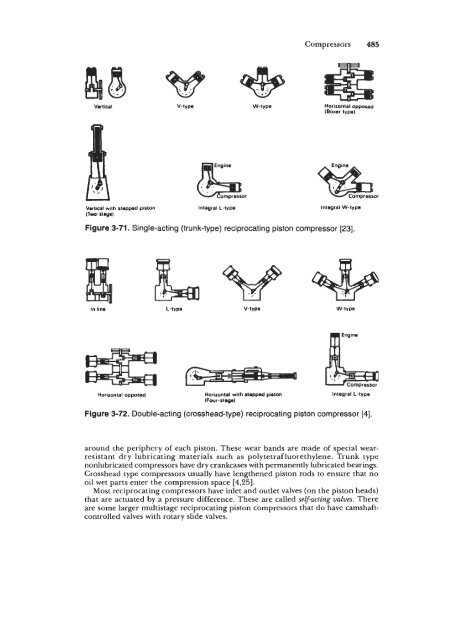
Compressors 485 

Vertical V-type W-type Horizontal opposed 

(Boxer type) 

Engine 

Vertical with stepped piston 

(Two-stagel 

Integral L-type 

Integral W-type 

Figure 3-71. Single-acting (trunk-type) reciprocating piston compressor [23]. 

or 

In line L-W.Ps V-type W-type 

Horizontal opposed 

Horizontal with stepped piston 

(Four-stage) 

Integral L-type 

Figure 3-72. Double-acting (crosshead-type) reciprocating piston compressor [4]. 

around the periphery of each piston. These wear bands are made of special wearresistant 

dry lubricating materials such as polytetrafluorethylene. Trunk type 

nonlubricated compressors have dry crankcases with permanently lubricated bearings. 

Crosshead type compressors usually have lengthened piston rods to ensure that no 

oil wet parts enter the compression space [4,25]. 

Most reciprocating compressors have inlet and outlet valves (on the piston heads) 

that are actuated by a pressure difference. These are called self-acting valves. There 

are some larger multistage reciprocating piston compressors that do have camshaftcontrolled 

valves with rotary slide valves.

486 Auxiliary Equipment 

The main advantage of the multistage reciprocating piston compressor is that there 

is nearly total positive control of the volumetric flowrate which can be put through 

the machine and the pressure of the output. Many reciprocative piston compressors 

allow for the rotation to be adjusted, thus, changing the throughput of air or gas. 

Also, providing adequate power from the prime mover, reciprocating piston 

compressors will automatically adjust to back pressure changes and maintain proper 

rotation speed. These compressors are capable of extremely high output pressure 

(see Figure 3-68). 

The main disadvantages to multistage reciprocating piston compressors is that they 

cannot be practically constructed in machines capable of volumetric flowrates much 

beyond 1,000 actual cfm. Also, the highercapacity compressors are rather large and 

bulky and generally require more maintenance than similar capacity rotary compressors. 

In a compressor, like a liquid pump, the real volume flowrate is smaller than the 

displacement volume. This is due to several factors. These are: 

pressure drop on the suction side 

heating up of the intake air 

internal and external leakage 

expansion of the gas trapped in the clearance volume (reciprocating piston 

compressors only) 

The first three factors are present in compressors, but they are small and on the 

whole can be neglected. The clearance volume problem, however, is unique to 

reciprocating piston compressors. The volumetric efficiency eV estimates the effect 

of clearance. The volumetric efficiency can be approximated as 

e, = 0.96[1- E(rf - l)] (3-76) 

where E = 0.04-0.12. Figure 3-73 gives values of the term in the brackets for various 

values of E and the rt. 

= 0.04 

= am 

= 0.08 

= 0.10 

= 0.12 

1 2 3 4 

pressure ratiopJp, 

= 0.14 

Figure 3-73. Volumetric efficiency for reciprocating piston compressors (with 

clearance) [4].

For a reciprocating piston compressor, Equation 3-70 becomes 


(3-77) 

Rotary Compressors 

Another important positive displacement compressor is the rotary compressor. 

This type of compressor is usually of rather simple construction, having no valves 

and being lightweight. These compressors are constructed to handle volumetric 

flowrates up to around 2,000 actual cfm and pressure ratios up to around 15 (see 

Figure 3-69). Rotary compressors are available in a variety of designs. The most widely 

used rotary compressors are sliding vane, rotary screw, rotary lobe, and liquid-piston. 

The most important characteristic of this type of compressors is that all have a 

fixed built-in pressure compression ratio for each stage of compression (as well as a 

fixed built-in volume displacement) [25]. Thus, at a given rate of rotational speed 

provided by the prime mover, there will be a predetermined volumetric flowrate 

through the compressor, and the pressure exiting the machine at the outlet will be 

equal to the design pressure ratio times the inlet pressure. 

If the back pressure on the outlet side of the compressor is below the fixed output 

pressure, the compressed gas will simply expand in an expansion tank or in the 

initial portion of the pipeline attached to the outlet side of the compressor. Figure 

3-74 shows the pressure versus volume plot for a typical rotary compressor 

operating against a back pressure below the design pressure of the compressor. 

If the back pressure on the outlet side of the compressor is equal to the fixed 

output pressure, then there is no expansion of the output gas in the initial portion of 

the expansion tank or the initial portion of the pipeline. 

Figure 3-75 shows the pressure versus volume plot for a typical rotary compressor 

operating against a back pressure equal to the design's pressure of the compressor. 

If the back pressure in the outlet side of the compressor is above the fixed output 

pressure, then the compressor must match this higher pressure at the outlet. In so 

doing the compressor cannot expel the compressed volume within the compressor 

efficiently. Thus, the fixed volumetric flowrate (at a given rotation speed) will be 

reduced from what it would be if the back pressure were equal to or less than the 

fixed output pressure. Figure 3-76 shows the pressure versus volume plot for a typical 

rotary compressor operating against a back pressure greater than the design pressure 

of the compressor. 

operabion below 

desion oresswe 

Operation at 

design pressure 

J- design pressure 

(discharge) 

a 

Volume 

Volume 

Figure 3-74. Rotary compressor with Figure 3-75. Rotary compressor with 

back pressure less than fixed 

back pressure equal to fixed pressure 

pressure output [4]. output [4].


Vdumo 

Figure 3-76. Rotary compressor with back pressure greater than fixed pressure 

output. 

Nearly all rotary compressors can be designed with multiple stages. Such multistage 

compressors are designed with nearly equal compression ratios for each stage. Thus, 

since the volumetric flowrate (in actual cfm) is smaller from one stage to the next, 

the volume displacement of each stage is progressively smaller. 

Sliding Vane Compressor 

The typical sliding vane compressor stage is a rotating cylinder located eccentrically 

in the bore of a cylindrical housing (see Figure 3-77). The vanes are in slots in the 

rotating cylinder, and are allowed to move in and out of these slots to adjust to 

the changing clearance between the outside surface of the rotating cylinder and the 

inside bore surface of the housing. The vanes are always in contact with the inside 

bore due to either air pressure under the vane, or spring force under the vane. The 

Figure 3-77. Sliding vane compressor [25].


top of the vanes slide over the inside surface of the bore of the housing as the inside 

cylinder rotates. Gas is brought into the compression stage through the inlet suction 

port. The gas is then trapped between the vanes, and as the inside cylinder rotates 

the gas is compressed to a smaller volume as the clearance is reduced. When the 

clearance is the smallest, the gas has rotated to the outlet port. The compressed gas 

is discharged to the pipeline system connected to the outlet side of the compressor. 

As each set of vanes reaches the outlet port, the gas trapped between the vanes is 

discharged. The clearance between the rotating cylinder and the housing is fixed, 

and thus the pressure ratio of compression for the stage is fixed, or built-in. The 

geometry, e.g., cylinder length, diameter, etc., of the inside of each compressor stage 

determines the displacement volume and compression ratio of the compressor. 

The principal seals within the sliding vane compressor are provided by the 

interface between the end of the vane and the inside surface of the cylindrical 

housing. The sliding vanes must be made of a material that will not damage the 

inside surface of the housing. Therefore, most vane material is phenolic resinimpregnated 

laminated fabrics (such as asbestos or cotton cloth). Also, some metals 

other than one that would gall with the housing can be used such as aluminum. 

Usually, vane compressors utilize oil lubricants in the compression cavity to allow 

for smooth action of the sliding vanes against the inside of the housing. There 

are, however, some sliding vane compressors that may be operated oil-free. These 

utilize bronze, or carbon/graphite vanes [25]. 

The volumetric flowrate for a sliding vane compression stage q, (ft”/min) is 

approximately 

q, = 2al (d, - mt)N (3-78) 

where a is the eccentricity in ft, 1 is the length of the cylinder in ft, d, is the outer 

diameter of the rotary cylinder in ft, 4 is the inside diameter of the cylindrical housing 

in ft, t is the vane thickness in ft, m is the number of vanes, and N is the speed of the 

rotating cylinder in rpm. 

The eccentricity a is 

a=- d, - d, 

2 

(3-79) 

Some typical values of a vane compressor stage geometry are dJd, = 0.88, a = 0.06d2, 

a = 0.06d2, and l/d, = 2.00 to 3.00. Typical vane up speed usually does not exceed 

50 ft/s. 

There is no clearance in a rotary compressor. However, there is leakage of air 

within the internal seal system and around the vanes. Thus, the typical volumetric 

efficiency for the sliding vane compression is of the order of 0.82 to 0.90. The heavier 

the gas, the greater the volumetric efficiency. The higher the pressure ratio through 

the stage, the lower the volumetric efficiency. 

Rotary Screw Compressor 

The typical rotary screw compressor stage is made up of two rotating shafts, or 

screws. One is a female rotor and the other a male rotor. These two rotating 

components turn counter to one another (counterrotating). The two rotating elements 

are designed so that as they rotate opposite to one another; their respective helix 

forms intermesh (see Figure 3-78). As with all rotary compressors, there are no valves. 

The gas is sucked into the inlet post and is squeezed between the male and female


female rotor 

male rotor 

Figure 3-78. Screw compressor working principle [4].


portion of the rotating intermeshing screw elements and their housing. The 

compression ratio of the stage and its volumetric flowrate are determined by the 

geometry of the two rotating screw elements and the speed at which they are rotated. 

Screw compressors operate at rather high speeds. Thus, they are rather high 

volumetric f lowrate compressors with relatively small exterior dimensions. 

Most rotary screw compressors use lubricating oil within the compression space. 

This oil is injected into the compression space and recovered, cooled, and recirculated. 

The lubricating oil has several functions 

seal the internal clearances 

cool the gas (usually air) during compression 

lubricate the rotors 

eliminate the need for timing gears 

There are versions of the rotary screw compressor that utilize water injection (rather 

than oil). The water accomplishes the same purposes as the oil, but the air delivered 

in these machines is oil-free. 

Some screw compressors have been designed to operate with an entirely oil-free 

compression space. Since the rotating elements of the compressor need not touch 

each other or the housing, lubrication can be eliminated. However, such rotary screw 

compressor designs require timing gears. These machines can deliver totally oil-free, 

water-free dry air (or gas). 

The screw compressor can be staged. Often screw compressors are utilized in threeor 

four-stage versions. 

Detailed calculations regarding the design of the rotary screw compressor are 

beyond the scope of this handbook. Additional details can be found in other 

references [4,25,26,27]. 

Rotary Lobe Compressor 

The rotary lobe compressor stage is a rather low-pressure machine. These 

compressors do not compress gas internally in a fixed sealed volume as in other 

rotaries. The straight lobe compressor uses two rotors that intermesh as they rotate 

(see Figure 3-79). The rotors are timed by a set of timing gears. The lobe shapes may 

be involute or cycloidal in form. The rotors may also have two or three lobes. As the 

rotors turn and pass the intake port, a volume of gas is trapped and carried between 

the lobes and the housing of the compressor. When the lobe pushes the gas toward 

the outlet port, the gas is compressed by the back pressure in the gas discharge line. 

Volumetric efficiency is determined by the leakage at tips of the lobes. The leakage 

is referred to as slip. Slippage is a function of rotor diameter, differential pressure, 

and the gas being compressed. 

For details concerning this low pressure compressor see other references [4,25,26,27]. 

Liquid Piston Compressor 

The liquid piston compressor utilizes a liquid ring as a piston to perform gas 

compression within the compression space. The liquid piston compressor stage 

uses a single rotating element that is located eccentrically inside a housing (see 

Figure 3-80). The rotor has a series of vanes extending radially from it with a slight 

curvature toward the direction of rotation. A liquid, such as oil, partially fills the 

compression space between the rotor and the housing walls. As rotation takes place, 

the liquid forms a ring as centrifugal forces and the vanes force the liquid to the 

outer boundary of the housing. Since the element is located eccentrically in the


Figure 3-79. Straight lobe rotary compressor operating cycle [4,23]. 

IN tnis SECTOR Liauio MOVES IN Tnis s 

0 OUTWARD - DdAWS OAS FROM @ INWARD- --.... . 

INLET WRTS INTO ROTOR 

IN ROTOR CHAM€ 

IN THIS SECT0 

COMPRESSED QAS 

ESCAPES AT DISCHARQL 

Figure 3-80. Liquid piston compressor [4,23]. 

housing, the liquid ring (or piston) moves in an oscillatory manner. The compression 

space in the center of the stage communicates with the gas inlet and outlet parts and 

allows a gas pocket. The liquid ring alternately uncovers the inlet part and the outlet 

part. As the system rotates, gas is brought into the pocket, compressed, and released 

to the outlet port. 

The liquid compressor has rather low efficiency, about 50%. The liquid piston 

compressor may be staged. The main advantage to this type of compressor is that it 

can be used to compress gases with significant liquid content in the stream.


Summary of Rotary Compressors 

The main advantage of rotary compressors is that most are easy to maintain in 

field conditions and in industrial settings. Also, they can be constructed to be rather 

portable since they have rather small exterior dimensions. Also, many versions of the 

rotary compressor can produce oil-free compressed gases. 

The main disadvantage are that these machines operate at a fued pressure ratio. 

Thus, the cost of operating the compressor does not basically change with reduced 

back pressure in the discharge line. As long as the back pressure is less than the 

pressure output of the rotary, the rotary will continue to operate at a fixed power 

level. Also, since the pressure ratio is built into the rotary compressor, discharging 

the compressor into a back pressure near or greater than the pressure output of the 

machine will significantly reduce the volumetic flowrate produced by the machine. 

Centrifugal Compressors 

The centrifugal compressor is the earliest developed dynamic, or continuous flow, 

compressor. This type of compressor has no distinct volume in which compression 

takes place. The main concept of the centrifugal compressor is use of centrifugal 

force to convert kinetic energy into pressure energy. Figure 3-81 shows a diagram of 

a single-stage centrifugal compressor. The gas to be compressed is sucked into the 

center of the rotating impeller. The impeller throws the gas out to the periphery by 

means of its radial blades and high-speed rotation. The gas is then guided through 

the diffuser where the high-velocity gas is slowed, which results in a high pressure. In 

multistage centrifugal compressors, the gas is passed to the next impeller after the 

diffuser of the previous impeller. In this manner, the compressor may be staged to 

OUT 

Figure 3-81. Single-stage centrifugal compressor [23].


increase the pressure of the ultimate discharge (see Figure 3-82). Since the compression 

pressure ratio at each stage is usually rather low, of the order 2 or so, the need for 

intercooling is not important after each stage. Figure 3-82 shows a typical multistage 

centrifugal compressor configuration with an intercooler after the first three stages 

of compression. 

The centrifugal compressor must operate at rather high rotation speeds to be 

effective. Most commercial centrifugal compressors operate at speeds of the order of 

20,000-30,000 rpm. With such rotation speeds very large volumes of gas can be compressed 

with equipment having rather modest external dimensions. Commercial 

centrifugal compressors can operate with volumetric flowrates up to around 10.4 

actual cfm and with overall compression ratios up to about 20. 

Centrifugal compressors are usually used in large processing plants and in some 

pipeline applications. They can be operated with any lubricant or other contaminant 

in the gas stream, or they can be operated with some small percentage of 

liquid in the gas stream. 

These machines are used principally to compress large volumetric f lowrates to 

rather modest pressures. Thus, their use is more applicable to the petroleum refining 

and chemical processing industries. 

More details regarding the centrifugal compressor may be found in other references 

[4,231. 

Axial-Flow Compressors 

The axial compressor is a very high-speed, large volumetric flowrate machine. 

This is another dynamics, or continuous flow machine. This type of compressor 

sucks in gas at the intake port and propels the gas axially through the compression 

space via a series of radially arranged rotor blades and stator (diffuser) blades (see 

Figure 3-83). As in the centrifugal compressor, the kinetic energy of the high-velocity 

flow exiting each rotor stage is converted to pressure energy in the follow-on stator 

(diffuser) stage. Axial-flow compressors have a volumetric flowrate range of about 

3 x 104-106 actual cfm. Their compression ratio is typically around 10 to 20. Because 

OUT 

Figure 3-82. Multistage centrifugal compressor with intercooling [23].

References 495 

Figure 3-83. Multistage axial-flow compressor [26]. 

of their small diameter, their machines are principal compressor design for jet engine 

applications. There are some applications for axial-f low compressors for large process 

plant operations where very large constant volumetric flowrates are needed. 

More detail regarding axial flow compressors may be found in other references 

[ 22,261. 

Prime Movers 

REFERENCES 

1. Kutz, M., Mechanical Enginem’Handbook, Twelfth Edition, John Wiley and Sons, 

New York, 1986. 

2. “API Specification for Internal-Combustion Reciprocating Engines for Oil-Field 

Service,” API STD 7B-llC, Eighth Edition, March 1981. 

3. “API Recommended Practice for Installation, Maintenance, and Operation of 

Internal-Combustion Engines,” API RP 7C-1 lF, Fourth Edition, April 1981. 

4. Atlas Copco Manual, Fourth Edition, 1982. 

5. Baumeister, T., Marks’ Standad Handbook for Mechanical En@nem, Seventh Edition, 

McCraw-Hill Book Co., New York, 1979. 

6. Moore, W. W., Fundamentals of Rotary Drilling, Energy Publications, 1981. 

7. “NEMA Standards, Motors and Generators,” ANSI/NEMA Standards Publication, 

NO. MG1-1978. 

8. Greenwood, D. G., Mechanical Power Tranmissions, McCraw-Hill Book Co., New 

York, 1962. 

9. Libby, C. C. Motor Section and Application, McCraw-Hill Book Co., New York, 1960. 

10. Fink, D. G., and Beaty, H. W., Standard Handbook for Electrical Engineers, Eleventh 

Edition, McGraw-Hill Book Co., New York, 1983. 

Power Transmission 

11. Hindhede, U., et al, Machine Design Fundamentals, J. Wiley and Sons, New York, 

1983. 

12. “API Specifications for Oil-Field V-Belting,” API Spec lB, Fifth Edition, March 

1978. 

13. Faulkner, L. L., and Menkes, S. B., Chainsfor Power Transmission and Materials 

Handling, Marcel Dekker, New York, 1982.


14. “Heavy Duty Offset Sidebar Power Transmission Roller Chain and Sprocket Teeth,“ 

ANSI Standard B 29.1, 29.10M-1981. 

15. “Inverted Tooth (Silent) Chains and Sprocket Teeth,” ANSI Standard B 29.2M- 

1982. 

16. “API Specifications for Oil Field Chain and Sprockets,” API Spec. 7E, Fourth 

Edition, February 1980. 

Pumps 

17. Karassik, I. J., et al., Pump Handbook, McGraw-Hill Book Co., New York, 1976. 

18. Matley, J., Fluid Movers; Pump CompressorS, Fans and Blowers, McGraw-Hill Book 

Co., New York, 1979. 

19. Gatlin, C., Petroleum Engineering: Drilling and Well Completions, Prentice-Hall, 

Englewood Cliffs, 1960. 

20. Hicks, T. G., Standard Handbook of Enginem’ng Calculations, Second Edition, McGraw- 

Hill Book Co., New York, 1985. 

21. Bourgoyne, A. T., et al., Applied Drilling Engineering, SPE, 1986. 

22. Hydraulics Institute Standards for Centrifugal, Rotary, and Reciprocating Pumps, 

Fourteenth Edition, 1983. 

Compressors 

23. Brown, R. N., Compressom: Selection and Ski% Gulf Publishing, 1986. 

24. Burghardt, M. D., Engineering Thermodynamics with Applications, Harper and Row, 

Second Edition, New York, 1982. 

25. Loomis, A. W., Cmpesed Air and Gas Data, Ingersoll-Rand Company, Third Edition, 

1980. 

26. Pichot, P., Compressor Application Engineering; Vol. 1: Compression Equipment, Gulf 

Publishing, 1986. 

27. Pichot, P., Compressor Application Engineering Vol. 2: Drivers for Rotating Equipment, 

Gulf Publishing, 1986.

Drilling and Well Completions 

Frederick E. Beck, Ph.D. 

ARC0 Alaska 

Anchorage, Alaska 

Daniel E. Boone 

Consultant, Petroleum Engineering 

Houston, Texas 

Robert DesBrandes, Ph.D. 

Louisiana State University 

Baton Rouge, Louisiana 

Phillip W. Johnson, Ph.D., P.E. 

University of Alabama 

Tuscaloosa, Alabama 

William C. Lyons, Ph.D., P.E. 

New Mexico Institute of Mining and Technology 

Socorro, New Mexico 

Stefan Miska, Ph.D. 

University of Tulsa 

Tulsa, Oklahoma 

Abdul Mujeeb 

Henkels & McCoy, Inc. 

Blue Bell, Pennsylvania 

Charles Nathan, Ph.D., P.E. 

Consultant, Corrosion Engineering 

Houston, Texas 

Chris S. Russell, P.E. 

Consultant, Environmental Engineering 

Las Cruces, New Mexico 

Ardeshir K. Shahraki, Ph.D. 

Dwight’s Energy Data, Inc. 

Richardson, Texas 

Andrzej K. Wojtanowicz, Ph.D., P.E. 

Louisiana State University 

Baton Rouge, Louisiana 

Derricks and Portable Masts ................................................................. 499 

Standard Derricks 501. Load Capacities 506. Design Loadings 508. Design Specifications 51 1. 

Maintenance and Use of Drilling and Well Servicing Structures 515. Derrick Efficiency Factor 521. 

Hoisting Systems ................................................................................... 523 

Drawworks 525. Drilling and Production Hoisting Equipment 530. Inspection 540. Hoist Tool 

Inspection and Maintenance Procedures 542. Wire Rope 544. 

Rotary Eauipment ................................................................................. 616 

Swivel and Rotary Hose 616. Drill-Stem Subs 619. Kelly 620. Rotary Table and Bushings 622. 

Mud Pumps ........................................................................................... 627 

Pump Installation 627. Pump Operation 630. Pump Performance Charts 631. Mud Pump 

Hydraulics 631. Useful Formulas 645. 

Drilling Muds and Completion Systems ............................................... 650 

Testing of Drilling Fluids 652. Composition and Applications 664. Oil-Based Mud Systems 675. 

Environmental Aspects 682. Typical Calculations in Mud Engineering 687. Solids Control 691. 

Mud-Related Hole Problems 695. Completion and Workover Fluids 701. 

Drill String: Composition and Design .................................................. 715 

Drill Collar 716. Drill Pipe 735. Tool Joints 748. Heavy-Weight Drill Pipe 749. Fatigue Damage 

of Drill Pipe 763. Drill String Design 765. 

Drilling Bits and Downhole Tools ........................................................ 769 

Classification of Drilling Bits 769. Roller Rock Bit 771. Bearing Design 774. Tooth Design 776. 

Steel Tooth Bit Selection 783. Diamond Bits 789. IADC Fixed Cutter Bit Classification System 801. 

Downhole Tools 812. Shock Absorbers 813. Jars. Underreamen 819. Stabilizers 823. 

497

498 Drilling and Well Completions 

Drilling Mud Hydraulics . ................... 829 

Rheological Classification of Drilling Fluids 829. Flow Regimes 830. Principle of Additive 

Pressures 834. Friction Pressure Loss Calculations 836. Pressure Loss Through Bit Nozzles 839. 

Air and Gas Drilling ............................................................................. 840 

Types of Operations 840. Equipment 844. Well Completion 847. Well Control 852. Air, Gas, and 

Unstable Foam Calculations 853. 

Downhole Motors................... ............................................................... 862 

Turbine Motors 863. Positive Displacement Motor 882. Special Applications 899. 

MWD and LWD ..................................................................................... 901 

MWD Technology 901. Directional Drilling Parameters 954. Safety Parameters 961. LWD 

Technology 971. Gamma and Ray Logs 971. Resistivity Logs 974. Neutron-Density Logs 985. 

Measuring While Tripping: Wiper Logs 999. Measurements at the Bit 1002. Basic Log 

Interpretation 1005. Drilling Mechanics 1015. Abnormal Pressure Detection 1036. Drilling Safety, 

Kick Alert 1067. Horizontal Drilling, Geosteering 1070. Comparison of LWD Logs with Wireline 

Logs 1077. Comparison of MWD Data with Other Drilling Data 1078. 

Directional Drilling .............................................................................. 1079 

Glossary 1079. Dogleg Severity (Hole Curvature) Calculations 1083. Deflection Tool 

Orientation 1085. ThreeDimensional Deflecting Model 1088. 

Selection of Drilling Practices ............................................................. 1090 

Factors Affecting Drilling Rates 1090. Selection of Weight on Bit, Rotary Speed, and Drilling 

Time 1091. Selection of Optimal Nozzle Size and Mud Flowrate 1097. 

Well Pressure Control .......................................................... ................ 1100 

Surface Equipment 1101. When and How to Close the Well 1101. Gas-Cut Mud 1103. The Closed 

Well 1105. Kick Control Procedures 1106. Maximum Casing/Borehole Pressure 11 11. 

Fishing Operations and Equipment ................................................... 1113 

Causes and Prevention 1114. Fishing Tools 11 15. Free Point 1124. 

Casing and Casing String Design ........................................................ 1127 

Types of Casing 1127. Casing Program Design 1128. Casing Data 1132. Elements of Threads 1141. 

Collapse Pressure 1147. Internal Yield Pressure 1155. Joint Strength 1156. Combination Casing 

Strings 1157. Running and Pulling Casing 1164. 

Well Cementing ................................................................................... 1177 

Cementing Principles 1179. Properties of Cement Slurry 1183. Cement Additives 1193. 

Primary Cementing 1200. *Diameter Casing Cementing 1211. Multistage Casing 

Cementing 1216. Secondary Cementing 1223. Squeeze Cementing 1224. Plug Cementing 1228. 

Tubing and Tubing String Design ....................................................... 1233 

API Physical Property Specification 1233. Dimension, Weights, and Lengths 1233. Running 

and Pulling Tubing 1239. Selection of Wall thickness and Steel Grade of Tubing 1251. Tubing 

Elongation/Contraction 1252. Packer--Tubing Force 1254. Permanent Corkscrewing 1257. 

Corrosion and Scaling ......................................................................... 1257 

Corrosion Theory 1259. Forms of Corrosion Attack 1268. Factors Influencing Corrosion 

Rate 1292. Corrodents in Drilling Fluids 1300. Corrosion Monitoring and Equipment Inspections 

1312. Corrosion Control 1323. Recommended Practices 1340. 

Environmental Considerations . . . . . .. .1343 

Site Assessment and Construction 1344. Environmental Concerns While in Operation 1352. 

Offshore Operations ............................................................................ 1363 

Drilling Vessels 1357. Marine Riser Systems. 1359. Casing Programs 1361. Well Control 1363. 

References ............................................................................................ 1373

- 


DERRICKS AND PORTABLE MASTS 

Derricks and portable masts provide the clearance and structural support 

necessary for raising and lowering drill pipe, casing, rod strings, etc., during 

drilling and servicing operations. Standard derricks are bolted together at the 

well site, and are considered nonportable. Portable derricks, which do not 

require full disassembly for transport, are termed masts. 

The derrick or mast must be designed to safely carry all loads that are likely 

to be used during the structure’s life [l]. The largest vertical dead load that 

will likely be imposed on the structure is the heaviest casing string run into the 

borehole. However, the largest vertical load imposed on the structure will result 

from pulling equipment (Le., drill string or casing string) stuck in the borehole. 

The most accepted method is to design a derrick or mast that can carry a dead 

load well beyond the maximum casing load expected. This can be accomplished 

by utilizing the safety factor. 

The derrick or mast must also be designed to withstand wind loads. Wind 

loads are imposed by the wind acting on the outer and inner surfaces of the 

open structure. When designing for wind loads, the designer must consider that 

the drill pipe or other tubulars may be out of the hole and stacked in the 

structure. This means that there will be loads imposed on the structure by the 

pipe weight (i.e., setback load) in addition to the additional loads imposed by 

the wind. The horizontal forces due to wind are counteracted by the lattice 

structure that is firmly secured to the structure’s foundation. Additional support 

to the structure can be accomplished by the guy lines attached to the structure 

and to a dead man anchor some distance away from it. The dead man anchor 

is buried in the ground to firmly support the tension loads in the guy line. The 

guy lines are pretensioned when attached to the dead man anchor. 

The API Standard 4F, First Edition, May 1, 1985, “API Specifications for 

Drilling and Well Servicing Structures,” was written to provide suitable steel 

structures for drilling and well servicing operations and to provide a uniform 

method of rating the structures for the petroleum industry. API Standard 4F 

supersedes API Standards 4A, 4D, and 4E thus, many structures in service today 

may not satisfy all of the requirements of API Standard 4F [2-51. 

For modern derrick and mast designs, API Standard 4F is the authoritative source 

of information, and much of this section is extracted directly from this standard. 

Drilling and well servicing structures that meet the requirements of API Standard 

4F are identified by a nameplate securely affixed to the structure in a conspicuous 

place. The nameplate markings convey at least the following information: 

Mast and Derrick Nameplate Information 

a. Manufacturer’s name 

b. Manufacturer’s address 

c. Specification 4F 

d. Serial number 

499


e. Height in feet 

f. Maximum rated static hook load in pounds, with guy lines if applicable, 

for stated number of lines to traveling block 

g. Maximum rated wind velocity in knots, with guy lines if applicable, with 

rated capacity of pipe racked 

h. The API specification and edition of the API specification under which 

the structure was designed and manufactured 

i. Manufacturer’s guying diagram-for structures as applicable 

j. Caution: Acceleration or impact, also setback and wind loads will reduce 

the maximum rated static hook load capacity 

k. Manufacturer’s load distribution diagram (which may be placed in mast 

instructions) 

1. Graph of maximum allowable static hook load versus wind velocity 

m.Mast setup distance for mast with guy lines. 

Substructure Nameplate information 

a. Manufacturer’s name 

b. Manufacture’s address 

c. Specification 4F 

d. Serial number 

e. Maximum rated static rotary capacity 

f. Maximum rated pipe setback capacity 

g. Maximum combined rated static rotary and rated setback capacity 

h. API specification and edition under which the structure was designed and 

manufactured. 

The manufacturer of structures that satisfy API Standard 4F must also furnish 

the purchaser with one set of instructions that covers operational features, block 

reeving diagram, and lubrication points for each drilling or well servicing 

structure. Instructions should include the raising and lowering of the mast and 

a facsimile of the API nameplate. 

Definitions 

Definitions and Abbreviations 

The following terms are commonly used in discussing derricks and masts: 

Crown block assembly: The stationary sheave or block assembly installed at the 

top of a derrick or mast. 

Derrick: A semipermanent structure of square or rectangular cross-section having 

members that are latticed or trussed on all four sides. This unit must be 

assembled in the vertical or operation position, as it includes no erection 

mechanism. It may or may not be guyed. 

Design load: The force or combination of forces that a structure is designed to 

withstand without exceeding the allowable stress in any member. 

Dynamic loading: The loading imposed upon a structure as a result of motion 

as opposed to static loading. 

Qnamic stress: The varying or fluctuating stress occurring in a structural member 

as a result of dynamic loading. 

Erection load: The load produced in the mast and its supporting structure during 

the raising and lowering operation.

Derricks and Portable Masts 501 

Guy line: A wire rope with one end attached to the derrick or mast assembly 

and the other end attached to a suitable anchor. 

Guying pattern: A plane view showing the manufacturer’s recommended loca-tions 

and distance to the anchors with respect to the wellhead. 

Height of derrick and mast without guy lines: The minimum clear vertical distance 

from the top of the working floor to the bottom of the crown block 

support beams. 

Height of mast with guy lines: The minimum vertical distance from the ground 

to the bottom of the crown block support beams. 

Impact loading: The loading resulting from sudden changes in the motion state 

of rig components. 

Mast: A structural tower comprising one or more sections assembled in a 

horizontal position near the ground and then raised to the operating position. 

If the unit contains two or more sections, it may be telescoped or unfolded 

during the erection. 

Mast setup distam: The distance from the centerline of the well to a designated point 

on the mast structure defined by a manufacturer to assist in the setup of the rig. 

Maximum rated static hook load: The sum of the weight applied at the hook and 

the traveling equipment for the designated location of the dead line anchor 

and the specified number of drilling lines without any pipe setback, sucker 

rod, or wind loadings. 

Pipe lean: The angle between the vertical and a typical stand of pipe with the setback. 

Racking platform: A platform located at a distance above the working floor for 

laterally supporting the upper end of racked pipe. 

Rated static rotary load: The maximum weight being supported by the rotary table 

support beams. 

Rated setback load: The maximum weight of tubular goods that the substructure 

can withstand in the setback area. 

Rod board. A platform located at a distance above the working floor for supporting 

rods. 

Static hook load: see Maximum Rated Static Hook Load. 

Abbreviations 

The following standard abbreviations are used throughout this section. 

ABS-American Bureau of Shipping 

AISC-American Institute of Steel Construction 

AISI-American Iron and Steel Institute 

ANSI-American National Standard Institute 

API-American Petroleum Institute 

ASA-American Standards Association 

ASTM-American Society for Testing and Materials 

AWS-American Welding Society 

IADC-International Association of Drilling Contractors 

SAE-Society of Automotive Engineers 

USAS-United States of America Standard (ANSI) 

RP-Recommended Practice 

Standard Derricks 

A standard derrick is a structure of square cross-section that dimensionally 

agrees with a derrick size shown in Table 41 with dimensions as designated in 

Figure 41.

~ 

Table 4-1 

Derrick Sizes and General Dimensions [2] 09 

1 2 3 4 5 6 7 

Nominal Draw works V Window 

Gin Pole 

Derrick Height Base Square Window Opening Opening Opening Clearance 

Size No. A B C C D E 

ft in. ft in. ft in. ft in. ft in. ft in. 

v C.. 

i 

F 

10- 

11 

12 

16 

18 

18A 

19 

20 

25 

~~ 

a 0 0 

87 0 

94 0 

122 0 

136 0 

136 0 

140 0 

147 0 

189 0 

20 0 

20 0 

24 0 

24 0 

26 0 

30 0 

30 0 

30 0 

37 6 

7 6 

7 6 

7 6 

7 6 

7 6 

7 6 

7 6 

7 6 

7 6 

23 8 

23 8 

23 8 

23 8 

23 8 

23 8 

26 6 

26 6 

26 6 

~ 

5 6 

5 6 

5 6 

5 6 

5 6 

5 6 

7 6 

6 6 

7 6 

8 0 

0 0 

8 0 

8 0 

12 0 

12 0 

17 0 

17 0 

17 0 

Tolerances: A, f 6 in.; B, f 5 in.; C, + 3 ft.. 6 in.: D. f 2 in.: E. k 6 in.


c 

I 

A 

A The vartical distance from the top of the base plate to 

the bottom of the crown block sumport beam. 

I Tha distance betwaan hael to heel of adidcant lags et the 

top of the base plate. 

C - The window opaninq measured In the clear and parallel to 

tha center line of the derrick ride from top of base plate. 

D - The sm+st clear dimension at the top of the derrick 

that would restrict passage of crown block. 

E - The eiaarence between the horixontal header of the pin 

poi. and the top of tha crown support beam. 

Derrick Window 

Flgure 4-1. Derrick dimensions [2]. 

The derrick window arrangement types A, C. D, and E, shown in Figure 4-2, 

shall be interchangeable. The sizes and general dimensions of the V window 

opening and drawworks window opening are given in Tables 4-1 and 4-2. 

Foundation Bolt Settings 

Foundation bolt sizes and patterns are shown in Figure 4-3. Minimum bolt 

sizes are used and should be increased if stresses dictate larger diameter. The 

(text conrinucd on page 506)


V- Window 

TYPE A 

M 

Ora w wor ks Window 

TYPE C 

Drawworks Window Ladder Window 

TYPE D 

TYPE E 

Figure 4-2. Derrick windows [2]. 

Table 4-2 

Conversion Values 

(For 0-50 Ft. Helght) [2] 

Wind Velocity 

Pressure 

P vk Wind Velocity 

Lb./Sq. Ft. Knots Miles Per Hour 

10 49 56 

15 60 69 

20 69 79 

25 77 89 

30 84 97 

35 91 105 

40 97 112 

45 103 119 

50 109 125 

55 114 131

~~ ~ 

Nominal 

Base Square 

Two I" or l-l/4" bolts at 

each corner 

1-3/8" holes in base plate 


TO" 2 118" rC- 

80- .87-, 94-, 122-, and 136-ft. Derricks 

Nominal 

Base Square 

Four 1-12'' bolts at 

each corner 

1-3/4"holes in base plate 

140 -ft. and 147-ft. Derricks 

Nominal : 

Base Square 

Four 2'' bolts at 

each corner 

2-3/8"Holes in base 

plate 

15": 1/8" 

* 4"-, 

189 -ft Derrick 

Figure 4-3. Foundation bolt pattern for derrick leg [2].


(text continued from page 503) 

maximum reaction (uplift, compression, and shear) produced by the standard 

derrick loading foundation bolt size and setting plan should be furnished to the 

original user, 

Load Capacities 

All derricks and masts will fail under an excessively large load. Thus API 

makes it a practice to provide standard ratings for derricks and masts that meet 

its specifications. The method for specifying standard ratings has changed over 

the years; therefore, old structures may fail under one rating scheme and new 

structures may fail under another. 

API Standard 4A (superseded by Standard 4F) provides rating of derrick 

capacities in terms of maximum safe load. This is simply the load capacity of a 

single leg multiplied by four. It does not account for pipe setback, wind loads, 

the number of lines between the crown block and the traveling block, the 

location of the dead line, or vibratory and impact loads. Thus, it is recommended 

that the maximum safe static load of derricks designed under Standard 

4A exceed the derrick load as follows: 

Derrick load* = 1.5(Wh + Wc + Wt + 4F,) (4-1) 

where W, = weight of the traveling block plus the weight of the drillstring 

suspended in the hole, corrected for buoyancy effects 

Wc = weight of the crown block 

W, = weight of tools suspended in the derrick 

F, = extra leg load produced by the placement of the dead and fast lines 

In general, F, = WJn if the deadline is attached to one of the derrick legs, 

and F, = WJPn if the deadline is attached between two derrick legs. n is the 

number of lines between the crown block and traveling block. The formula for 

F, assumes that no single leg shares the deadline and fastline loads. 

The value of 1.5 is a safety factor to accommodate impact and vibration loads. 

Equation 4-1 does not account for wind and setback loads, thus, it may provide 

too low an estimate of the derrick load in extreme cases. 

API Standard 4D (also superseded by Standard 4F) provides rating of portable 

masts as follows: 

For each mast, the manufacturer shall designate a maximum rated static hook 

load for each of the designated line reevings to the traveling block. Each load 

shall be the maximum static load applied at the hook, for the designated location 

of deadline anchor and in the absence of any pipe-setback, sucker-rod, or wind 

loadings. The rated static hook load includes the weight of the traveling block 

and hook. The angle of mast lean and the specified minimum load guy line 

pattern shall be considered for guyed masts. 

Under the rigging conditions given on the nameplate, and in the absence of 

setback or wind loads, the static hook load under which failure may occur in 

masts conforming to this specification can be given as only approximately twice 

the maximum rated static hook load capacity. 

*This is an API Standard 4A rating capacity and should not be confused with the actual derrick load 

that will be discussed in the section titled "Derricks and Portable Masts."


The manufacturer shall establish the reduced rated static hook loads for the 

same conditions under which the maximum rated static hook loads apply, but 

with the addition of the pipe-setback and sucker-rod loadings. The reduced rated 

static hook loads shall be expressed as percentages of the maximum rated static 

hook loads. Thus, the portable mast ratings in Standard 4D include a safety 

factor of 2 to allow for wind and impact loads, and require the manufacturer 

to specify further capacity reductions due to setback. 

The policy of Standard 4D, that the manufacturer specify the structure load 

capacity for various loading configurations, has been applied in detail in 

Standards 4E (superseded by Standard 4F) and 4F. Standard 4F calls for detailed 

capacity ratings that allow the user to look up the rating for a specific loading 

configuration. These required ratings are as follows. 

Standard Ratings 

Each structure shall be rated for the following applicable loading conditions. 

The structures shall be designed to meet or exceed these conditions in 

accordance with the applicable specifications set forth herein. The following 

ratings do not include any allowance for impact. Acceleration, impact, setback, 

and wind loads will reduce the rated static hook load capacity. 

Derrlck-Stationary 

Base 

1. Maximum rated static hook load for a specified number of lines to the 

traveling block. 

2. Maximum rated wind velocity (knots) without pipe setback. 

3. Maximum rated wind velocity (knots) with full pipe setback. 

4. Maximum number of stands and size of pipe in full setback. 

5. Maximum rated gin pole capacity. 

6. Rated static hook load for wind velocities varying from zero to maximum 

rated wind velocity with full rated setback and with maximum number of 

lines to the traveling block. 

Mast with Guy Lines 

1. Maximum rated static hook load capacity for a specified number of lines 

strung to the traveling block and the manufacturer’s specified guying. 




Mast wlthout Guy Lines 






5. Rated static hook load for wind velocities varying from zero to maximum 

rated wind velocity with full rated setback and with maximum number of 

lines to the traveling block.


Mast and Derricks under Dynamic Conditions 



2. Hook load, wind load, vessel motions, and pipe setback in combination with 

each other for the following: 

a. Operating with partial setback. 

b. Running casing. 

c. Waiting on weather. 

d. Survival. 

e. Transit. 

Substructures 

1. Maximum rated static hook load, if applicable. 

2. Maximum rated pipe setback load. 

3. Maximum rated static load on rotary table beams. 

4. Maximum rated combined load of setback and rotary table beams. 

Substructure under Dynamic Conditions 

1. Maximum rated static hook load. 

2. Maximum rated pipe setback load. 

3. Maximum rated load on rotary table beams. 

4. Maximum rated combined load of setback and rotary table beams. 

5. All ratings in the section titled “Mast and Derricks under Dynamic Conditions.” 

Design Loadings 

Derricks and masts are designed to withstand some minimum loads or set of 

loads without failure. Each structure shall be designed for the following 

applicable loading conditions. The structure shall be designed to meet or exceed 

these conditions in accordance with the applicable specifications set forth herein. 

Derrick-Stationary 

Base 

1. Operating loads (no wind loads) composed of the following loads in 

combination: 

a. Maximum rated static hook load for each applicable string up condition. 

b. Dead load of derrick assembly. 

2. Wind load without pipe setback composed of the following loads in 

combination: 

a. Wind load on derrick, derived from maximum rated wind velocity 

without setback (minimum wind velocity for API standard derrick sizes 

10 through 18A is 93 knots, and for sizes 19 through 25 is 107 knots). 

b. Dead load of derrick assembly. 

3. Wind load with rated pipe setback composed of the following loads in 

combination: 

a. Wind load on derrick derived from maximum rated wind velocity with 

setback of not less than 93 knots. 

b. Dead load of derrick assembly.


c. Horizontal load at racking platform, derived from maximum rated wind 

velocity with setback of not less than 93 knots acting on full pipe 

setback. 

d. Horizontal load at racking platform from pipe lean. 

Mast with Guy Lines 

1. Operating loads (no wind load) composed of the following loads in 

combination: 


b. Dead load of mast assembly. 

c. Horizontal and vertical components of guy line loading. 

2. Wind loads composed of the following loads in combination: 

a. Wind load on mast, derived from a maximum rated wind velocity with 



c. Horizontal loading at racking board, derived from a maximum rated 

wind velocity with setback of not less than 60 knots, acting on full pipe 

setback. 

d. Horizontal and vertical components of guy line loading. 

e. Horizontal and vertical loading at rod board, derived from a maximum 

rated wind velocity with setback of not less than 60 knots, acting on 

rods in conjunction with dead weight of rods. 


a. Wind load on mast, derived from a maximum rated wind velocity with 



c. Horizontal loading at racking platform, derived from a maximum rated 

wind velocity with setback of not less than 60 knots, acting on full pipe 

setback. 

d. Horizontal and vertical components of guy line loading. 


a. Wind load on mast derived from a maximum rated wind velocity without 



c. Horizontal and vertical components of guy line loading. 

5. Erection loads (zero wind load) composed of the following loads in 

combination: 

a. Forces applied to mast and supporting structure created by raising or 

lowering mast. 


6. Guy line loading (assume ground anchor pattern consistent with manufacturer’s 

guying diagram shown on the nameplate). 

a. Maximum horizontal and vertical reactions from conditions of loading 

applied to guy line. 

b. Dead load of guy line. 

c. Initial tension in guy line specified by mast manufacturer. 

Mast without Guy Lines 

1. Operating loads composed of the following loads in combination: 


b. Dead load of mast assembly.


2. Wind load without pipe setback composed of the following loads in 

combination: 

a. Wind loading on mast, derived from a maximum rated wind velocity 

without setback of not less than 93 knots. 


3. Wind load with pipe setback composed of the following loads in combination: 

a. Wind loading on mast, derived from a maximum rated wind velocity 

with setback of not less than 70 knots. 


c. Horizontal load at racking platform derived from a maximum rated wind 

velocity with setback of not less than 70 knots acting on pipe setback. 

d. Horizontal load at racking platform from pipe lean. 

4. Mast erection loads (zero wind load) composed of the following loads in 

combination: 

a. Forces applied to mast and supporting structure created by raising or 

lowering mast. 


5. Mast handling loads (mast assembly supported at its extreme ends). 

Derricks and Mast under Dynamic Conditions 

All conditions listed in the section titled “Load Capacities,” subsection titled 

“Mast and Derricks under Dynamic Conditions,” are to be specified by the user. 

Forces resulting from wind and vessel motion are to be calculated in accordance 

with the formulas presented in the section titled “Design Specifications,” 

paragraphs titled “Wind,” “Dynamic Loading (Induced by Floating Hull Motion).” 

Substructures 

1. Erection of mast, if applicable. 

2. Moving or skidding, if applicable. 

3. Substructure shall be designed for the following conditions: 

a. Maximum rated static rotary load. 

b. Maximum rated setback load. 

c. Maximum rated static hook load (where applicable). 

d. Maximum combined rated static hook and rated setback loads (where 

applicable). 

e. Maximum combined rated static rotary and rated setback loads. 

f. Wind loads resulting from maximum rated wind velocity acting from any 

direction on all exposed elements. Wind pressures and resultant forces 

are to be calculated in accordance with the equations and tables in the 

section titled “Design Specifications,” paragraph titled “Wind.” When 

a substructure is utilized to react guy lines to the mast, these reactions 

from the guy lines must be designed into the substructure. 

g. Dead load of all components in combination with all of the above. 

Substructure under Dynamic Conditions 

All conditions listed in the section titled “Load Capacities,” paragraph titled 

“Structure under Dynamic Conditions,’’ are to be specified by the user. Forces 

resulting from wind and vessel motion are to be calculated in accordance with 

formulas from the section titled “Design Specifications,” paragraphs titled 

“Wind” and “Dynamic Loading (Induced by Floating Hull Motion).”

Design Specifications 


In addition to withstanding some minimum load or loads (sections titled 

“Load Capacities” and “Design Specifications”), derricks and masts that satisfy 

API standards must also satisfy certain requirements regarding materials, 

allowable stresses, wind, dynamic loading, earthquakes and extremes of temperature. 

Materials 

The unrestricted material acceptance is not intended since physical properties 

are not the sole measure of acceptability. Metallurgical properties, which affect 

fabrication and serviceability, must also be considered. 

Steel. Steel shall conform to one of the applicable ASTM specifications referred 

to by applicable AISC specifications. Other steels not covered by these specifications 

may be used provided that the chemical and physical properties conform 

to the limits guaranteed by the steel manufacturer. Structural steel shapes having 

specified minimum yield less than 33,000 psi shall not be used. Certified mill 

test report or certified reports of tests made in accordance with ASTM A6 and 

the governing specification shall constitute evidence of conformity with one of 

the specifications listed. 

Bolts. Bolts shall conform to one of the applicable SAE, ASTM, or AISC 

specifications. Other bolts not covered by these specifications may be used 

provided the chemical, mechanical, and physical properties conform to the limits 

guaranteed by the bolt manufacturer. Certified reports shall constitute sufficient 

evidence of conformity with the specification. Bolts of different mechanical 

properties and of the same diameter shall not be mixed on the same drilling 

or servicing structure to avoid the possibility of bolts of relatively low strength 

being used where bolts of relatively high strength are required. 

Welding Electrodes. Welding electrodes shall conform to applicable AWS and 

ASTM specifications or other governing codes. Newly developed welding 

processes shall use welding electrodes conforming to applicable AWS or other 

governing publications. Certified reports shall constitute sufficient evidence of 

conformity with the specifications. 

Wire Rope. Wire rope for guy lines or erection purposes shall conform to API 

Specification 9A “Specification for Wire Rope.” 

Nonferrous Materiais. Nonferrous materials must conform to appropriate 

governing codes. Certified reports shall constitute sufficient evidence of 

conformity with such codes. 

Allowable Stresses 

AISC specifications for the design fabrication and erection of structural steel 

for buildings shall govern the design of these steel structures (for AISC 

specifications, see the current edition of Steel Construction Manual of the 

American Institute of Steel Construction). Only Part I of the AISC manual, the 

portion commonly referred to as elastic design, shall be used in determining 

allowable unit stresses; use of Part 11, which is commonly referred to as plastic


design, is not allowed. The AISC shall be the final authority for determination 

of allowable unit stresses, except that current practice and experience do not 

dictate the need to follow the AISC for members and connections subject to 

repeated variations of stress, and for the consideration of secondary stresses. 

For purposes of this specification, stresses in the individual members of a 

latticed or trussed structure resulting from elastic deformation and rigidity of 

joints are defined as secondary stresses. These secondary stresses may be taken 

to be the difference between stresses from an analysis assuming fully rigid joints, 

with loads applied only at the joints, and stresses from a similar analysis with 

pinned joints. Stresses arising from eccentric joint connections, or from 

transverse loading of members between joints, or from applied moments, must 

be considered primary stresses. 

Allowable unit stresses may be increased 20% from the basic allowable stress when 

secondary stresses are computed and added to the primary stresses in individual 

members. However, primary stresses shall not exceed the basic allowable stresses. 

Wind and Dynamic Stresses (Induced by Floating Hull Motion). Allowable 

unit stresses may be increased one-third over basic allowable stresses when 

produced by wind or dynamic loading, acting alone, or in combination with the 

design dead load and live loads, provided the required section computed on 

this basis is not less than required for the design dead and live loads and impact 

(if any), computed without the one-third increase. 

Wire Rope. The size and type of wire rope shall be as specified in API 

Specification 9A and by API RP 9B (see section titled “Hoisting System”). 

1. A mast raised and lowered by wire rope shall have the wire rope sized to 

have a nominal strength of at least 2+ times the maximum load on the 

line during erection. 

2. A mast or derrick guyed by means of a wire rope shall have the wire rope 

sized so as to have a nominal strength of at least 24 times the maximum 

guy load resulting from a loading condition. 

Crown Shafting. Crown shafts, including fastline and deadline sheave support 

shafts, shall be designed to AISC specifications except that the safety factor in 

bending shall be a minimum of 1.67 to yield. Wire rope sheaves and bearings 

shall be designed in accordance with “API Specification 8A: Drilling and 

Production Hoisting Equipment.” 

Wind 

Wind forces shall be applied to the entire structure. The wind directions that 

result in the highest stresses for each component of the structure must be 

determined and considered. Wind forces for the various wind speeds shall be 

calculated according to 

F = (PI (A) (4-2) 

where F = Force in lb 

P = Pressure in lb/ft2 

A = Total area, in ftp, projected on a plane, perpendicular to the direction 

of the wind, except that the exposed areas of two opposite sides of 

the mast or derrick shall be used.


When pipe or tubing is racked in more than one area, the minimum area of 

setback shall be no less than 120% of the area on one side; when rods are racked 

on more than one area, the minimum area of rods shall be no less than 150% 

of the area of one side to account for the effect of wind on the leeward area 

(Figure 4-4). 

The pressure due to wind is 

P = 0.00338 (V;)(C,)(C,) (4-3) 

where P = pressure in. lb/ft4 

V, = wind velocity in knots 

C, = height coefficient 

Height (ft) c, 

0- 50 1 .o 

50-1 00 1.1 

100-1 50 1.2 

150-200 1.3 

200-250 1.4 

NOTE: In calculating the value of A, 

If R is greater than lSa, use R. If not, use 1.5a. 

If T is greater than 1.2b, use T. If not, use 1.2b. 

Figure 4-4. Diagram of projected area [9].


Height is the vertical distance from ground or water surface to the center of 

area. The shape coefficient Cs for a derrick is assumed as 1.25. Cs and C, were 

obtained from ABS, "Rules for Building and Classing Offshore Drilling Units, 1968." 

Dynamic Loading (Induced by Floating Hull Motion) 

Forces shall be calculated according to the following [6]: 

FP = (&)[ $)( $) + w sine 

(4-5) 

where W = dead weight of the point under consideration 

L, = distance from pitch axis to the gravity center of the point under 

consideration in feet 

L = distance from roll axis to the gravity center of the point under 

consideration in feet 

H = heave (total displacement) 

T, = period of pitch in seconds 

Tr = period of roll in seconds 

Th = period of heave in seconds 

I$ = angle of pitch in degrees 

8 = angle of roll in degrees 

g = gravity in 32.2 ft/s/s 

Unless specified, the force due to combined roll, pitch, and heave shall be 

considered to be the largest of the following: 

1. Force due to roll plus force due to heave. 

2. Force due to pitch plus force due to heave. 

3. Force due to roll and pitch determined as the square root of the sum of 

squares plus force due to heave. 

Angle of roll or pitch is the angle to one side from vertical. The period is for 

a complete cycle. 

Earthquake 

Earthquake is a special loading condition to be addressed when requested by 

the user. The user is responsible for furnishing the design criteria that includes 

design loading, design analysis method, and allowable response. 

The design criteria for land units may be in accordance with local building 

codes using equivalent static design methods. 

For fixed offshore platform units, the design method should follow the 

strength level analysis guidelines in API RP 2A. The drilling and well servicing 

units should be able to resist the deck movement, i.e., the response of the deck


to the ground motion prescribed for the design of the offshore platform. The 

allowable stresses for the combination of earthquake, gravity and operational 

loading should be limited to those basic allowables with the one-third increase 

as specified in AISC Part I. The computed stresses should include the primary 

and the secondary stress components. 

Extreme Temperature 

Because of the effect of low temperatures on structural steel, it will be no 

use to change (decrease) the allowable unit stresses mentioned in the preceding 

paragraphs titled “Allowable Stresses.” Low temperature phenomena in steel 

are well established in principle. Structures to be used under extreme conditions 

should use special materials that have been, and are being, developed for 

this application. 

Miscellaneous 

Structural Steels. Structures shall conform to sections of the AISC “Specifications 

for the Design, Fabrication and Erection of Structural Steel Buildings.” 

Castings. All castings shall be thoroughly cleaned, and all cored holes shall be 

drifted to ensure free passage of proper size bolt. 

Protection. Forged parts, rolled structural steel shapes and plates, and castings 

shall be cleaned, primed, and painted with a good commercial paint or other 

specified coating before shipment. Machined surfaces shall be protected with a 

suitable lubricant or compound. 

Socketing. Socketing of raising, erecting, or telescoping mast wire ropes shall 

be performed in accordance with practices outlined by API RP 9B. 

Recommended Practice for Maintenance and 

Use of Drilling and Well Servicing Structures 

These general recommendations, if followed, should result in longer satisfactory 

service from the equipment. These recommendations should in every 

case be considered as supplemental to, and not as a substitute for, the manufacturer’s 

instructions. 

The safe operation of the drilling and well servicing structure and the success 

of the drilling operation depend on whether the foundation is adequate for the 

load imposed. The design load for foundation should be the sum of the weight 

of the drilling or well servicing structure, the weight of the machinery and 

equipment on it, the maximum hook load of the structure, and the maximum 

setback load. 

Consultation with the manufacturer for approval of materials and methods 

is required before proceeding with repairs. Any bent or otherwise damaged 

member should be repaired or replaced. Any damaged compression member 

should be replaced rather than repaired by straightening. Drilling and well 

servicing structures use high-strength steels that require specific welding electrodes 

and welding techniques. 

Fixtures and accessories are preferably attached to a structure by suitable 

clamps. Do not drill or burn holes in any members or perform any welding 

without obtaining approval of the manufacturer.


Wire line slings or tag lines should have suitable fittings to prevent the rope 

from being bent over sharp edges and damaged. 

Loads due to impact, acceleration, and deceleration niay be indicated by 

fluctuation of the weight indicator readings and the operator should keep the 

indicator readings within the required hook load capacity. 

In the erecting and lowering operation, the slowest practical line speed should 

be used. 

Girts, braces, and other members should not, under any circumstances, be 

removed from the derrick while it is under load. 

The drilling and well servicing structure manufacturer has carefully designed 

and selected materials for his or her portable mast. The mast should perform 

satisfactorily within the stipulated load capacities and in accordance with the 

instructions. Every operator should study the instructions and be prepared for 

erecting, lowering, and using the mast. 

The substructure should be restrained against uplift, if necessary, by a suitable 

dead weight or a hold-down anchor. The weight of the hoist and vehicle, where 

applicable, may be considered as part or all of the required anchorage. 

Each part of a bolted structure is designed to carry its share of the load; 

therefore, parts omitted or improperly placed may contribute to the structure 

failure. In the erection of bolted structures, the bolts should be tightened only 

slightly tighter than finger-tight. After the erection of the structure is completed, 

all bolts should be drawn tight. This procedure permits correct alignment of 

the structure and results in proper load distribution. 

Sling Line inspection and Replacement 

One or more of the three principal factors, including wear due to operation, 

corrosion and incidental damage, may limit the life of a sling. The first may be 

a function of the times the mast is raised, and the second will be related to 

time and atmospheric conditions. The third will bear no relation to either, since 

incidental damage may occur at the first location as well as any other. 

Charting of sling line replacement shows an erratic pattern. Some require 

replacement at a relatively early date and others last several years longer. Early 

replacements generally show incidental damage, and it is possible that some of 

the longer lived ones are used beyond the time when they should be replaced. 

There is no way of judging the remaining strength of a rusty rope; therefore, 

rusty sling lines should be replaced. Areas adjacent to end connections should 

be examined closely for any evidence of corrosion. 

It would no doubt be possible to establish a normal sling line life expectancy in 

terms of the number of locations used, as long as a set number of months was not 

exceeded. However, this would not preclude the necessity for careful inspection to 

guard against incidental damage. A line with any broken wires should be replaced. 

A line showing any material reduction of metal area from abrasion should be 

replaced. A line showing kinking, crushing, or other damage should be replaced. 

Replacement of lines based on normal life expectancy will provide some 

degree of safety, but it is important that such provisions do not cause any degree 

of laxity in sling line inspection. 

Sling lines should be well lubricated. The field lubricant should be compatible 

with the original lubricant, and to this end the rope manufacturer should be 

consulted. The object of rope lubrication is to reduce internal friction and to 

prevent corrosion. 

The following routine checks, as applicable, should be made at appropriate 

intervals:


1. Inspect welds in erecting mechanism for cracks and other signs of 

deformity. 

2. Follow the manufacturer’s instructions in checking hydraulic circuits 

before lowering operation. Make sure of adequate supply of hydraulic 

fluid. 

3. Wire rope, including operating lines, raising lines, and guy lines, should 

be inspected for kinks, broken wires, or other damage. Make certain that 

guy lines are not fouled and that other lines are in place in sheave grooves 

before raising or lowering operation. 

4. Check safety latches and guides in telescoping mast for free operation 

before lowering operation. Keep latches and guides clean and properly 

lubricated. 

5. Check unit for level and check foundation and supports for correct 

placement before erecting operation. 

6. Check lubrication of crown sheaves. 

7. Check lubrication and condition of bearings in all sheaves, sprockets, etc. 

8. Check folding ladders for free operation before lowering operation. 

9. During drilling operations, it is advisable to make scheduled inspections 

of all bolted connections to ensure that they are tight. 

10. The visual field inspection of derrick or mast and substructure procedure 

is recommended for use by operating personnel (or a designated representative) 

to the extent that its use satisfies conditions for which an 

inspection is intended. A sample report form for this inspection procedure 

can be found in API Standard 4F. Forms are also available from International 

Association of Drilling Contractors (IADC). 

Splicing locks should be checked frequently for locking position or tightness, 

preferably on each tour during drilling operations. To develop its rated load 

capacity, the axis of the structure must be in alignment throughout its length. 

It is important that any splice mechanism or locks be maintained in such 

condition as to ensure structure alignment. 

Guying for Portable Masts with Guy Llnes 

This recommendation is applicable for most conditions encountered in the 

use of this type mast. There will be exceptions where location clearance, ground 

conditions, or other unusual circumstances require special considerations. Figure 

4-5 shows a recommended guying pattern that may be used under general 

conditions in the absence of an authorized API manufacturer’s recommendations. 

Guy lines should be maintained in good condition, free from rust, 

corrosion, frays, and kinks. Old sand line is not recommended for guy lines. 

All chains, boomers, clamps, and tensioning devices used in the guy lines shall 

satisfy the mast manufacturer’s recommendations. In the absence of mast 

manufacturer’s recommendations, the following minimum breaking strengths 

should be maintained: load guy lines-1 8 tons; external guy lines-12 tons; 

racking board guy lines-10 tons. 

Guy Line Anchors for Portable Masts with Guy Lines 

Guy line anchors including expanding anchors, concrete deadmen, or any 

other approved techniques are acceptable. The soil condition may determine 

the most applicable type. Recommendations for anchor design and testing 

are as follows:


A = Four crown to ground guys. Minimum guyline size recommended as 5/8" unless 

otherwise specified by mast manufacturer. Tensioning may be judged by catenary 

(sag). 6" catenary (approximately 1,000 Ib tension) recommended on initial 

tensioning. 

B = Two racking board to board guys. Minimum guyline size recommended is 9/16" 

unless otherwise specified by mast manufacturer. 12"-18" catenary (approximately 

500 Ib tension) recommended on initial tensioning. 

C = Two additional racking board guys to ground. Recommended when winds are in 

excess of design magnitude (name plate rating) or when pipe set back exceeds 

rated racking capacity or when weather protection is used on board. Minimum 

guyline size recommended is 9/16" unless otherwise specified by mast manufacturer. 

6"-12" catenary (approximately 1,000 Ib tension) recommended on initial 

tensioning. 

D = Two or four intermediate mast to ground guys. Recommended at option of mast 

manufacturer only. Minimum guyline size recommended is 5/8" unless otherwise 

specified by mast manufacturer. 6"-12" catenary (approximately 1,000 Ib tension) 

recommended on initial tensioning. 

CAUTION: WHEN THE TWO "A LINES ON THE DRAWWORKS SIDE OF THE MAST 

ARE USED AS LOAD GUYS, THE MINIMUM LINE SIZE SHALL BE 3/4" IPS 6 x 31 

CLASS OR BETTER, AND THE "2" DIMENSION SHALL NOT BE LESS THAN 60'. 

Figure 4-5. Recommended guying pattern-general conditions [3].


All guy line anchors should have a minimum breaking or pull-out strength 

at least equal to two times the maximum total calculated anchor load in 

the direction of the resultant load, and in the absence of manufacturer's 

recommendations, values in Table 4-3 are recommended. 

Representative pull tests for the area, size, and type of anchor involved and 

made by recognized testing methods should be made and recorded. Records 

should be maintained by the installer for temporary anchors and by the 

lease owner for permanent anchors. Permanent anchors should be visually 

inspected prior to use. If damage or deterioration is apparent, the anchor 

should be tested. 

Metal components of anchors should be galvanized or otherwise protected 

against corrosion. Sucker rods should not be used in anchor construction. 

Anchor location should be marked with a stake if projections aboveground 

are subject to bending or other abuse. 

Anchor location should avoid old pit or other disturbed areas. 

Mast Foundation for Portable Masts with Guy Lines 

Foundations must consider ground conditions, location preparation, and 

supplemental footing as required to provide a stable base for mast erection and 

to support the mast during the most extreme loading encountered. A recommended 

location preparation to provide ground conditions for safe operations 

is shown in Figure 4-6. 

Supplemental Footing 

Supplemental footing must be provided to distribute the concentrated loads 

from the mast and mast mount to the ground. The manufacturer's load distribution 

diagram indicates the magnitude and location of these concentrated loads. 

If the manufacturer's load distribution diagram is not available, supplemental 

footing should be provided to carry the maximum hook load encountered, plus 

the gross weight of mast and mast mount weight during mast erection. The area 

Table 4-3 

Recommended Guyline Anchor Spacing and Loads 

See Par. C. 16a and Figure C.l [3] 

1 2 3 4 5 6 7 

Doublca Mast Singles Mast Pole Mast 

Mini m u m . 

Spacing Anchor Anchor Anchor 

X or Y Test Angle Test Angle Test Angle 

Dimeniion Anchor from Horir. Anchor from Horiz. Anchor from Horir. 

See Fig. A.1. Test had, to Well Test Load, to Well Test Load, to Well 

feet ton8 Center Line tons Center Line tons Center Line 

20 

N.A. N.A. 3.7 70' 

7.0 67' 

25 15.6 71' 

- - 

- - 

30 13.7 67O 3.1 609 - - 

40 11.0 600 2.8 530 4.0 49' 

60 8.4 499 2.7 45- 35 

45- 

70 7.8 450 2.7 450 - - 

80 

7.4 45' 2.7 450 3.0 450 

w 7.0 450 2.7 450 

- 

50 9.3 540 27 45. - - 

NOTE: Prefemd. X pnater than Y. Limita, Y nawt not 

emeed I.2SXand Z mmt be eplial to bz leas than 

1.SX bid notlrm than Y. (Fig. C.1) 

CAUTION THE ADDITION OP WINDSCREENS 

OR THE RACKING OF PIPE ABOVE 

GROUND LEVEL CAN SICNIFI- 

CANTLY INCREASE THE ABOVE


Second Preference 

-0 

- 

+I 

+I 

I 

-%Deadman 

7 Tons 

Capacity 

t 

'1 

T 

Grade 1:20 max 

............ 

Load Bearing Area: Compacted sand or gravel requiring picking for removal or better 

base. Safe bearing capacity desired-Min., 8000 psf, level and drained. Rig Location 

Area: May grade away from well along centerline II at ma. drop of 1:20. Should be 

level across grades parallel to centerline 1. Safe bearing capacity desired-min., 6000 

psf. Allow maneuvering entry for drive in or back in. Drainage of entire area required. 

See Table 4-3. 

Figure 4-6. Portable mast location preparation 131.


and type of supplemental footing must ensure that the safe bearing capacity of 

soils on location is not exceeded. 

Precautions and Procedures tor Low-Temperature Operations 

A survey of 13 drilling contractors operating 193 drilling rigs in northern 

Canada and Alaska indicated that there is a wide range of experience and 

operating practices under extremely low-temperature conditions. A sizable 

number of portable masts failed in the lowering or raising process in winter. 

Thus the exposure to low-temperature failures focuses on mast lowering and 

raising operations. Based on reports, however, this operation has been 

accomplished successfully in temperatures as low as -50°F. While the risk may 

be considerably greater because of the change in physical characteristics of steel 

at low temperatures, operators may carry on “normal” operations even at 

extremely low temperatures. This may be accomplished by closely controlled 

inspection procedures and careful handling and operation to reduce damage and 

impact loading during raising and lowering operations. At present, there seems 

to be no widely accepted or soundly supported basis for establishing a critical 

temperature for limiting the use of these oilfield structures. Experience in the 

operation of trucks and other heavy equipment exposed to impact forces 

indicates that -40°F may be the threshold of the temperature range, at which 

the risk of structural failure may increase rapidly. Precautionary measures should 

be more rigidly practiced at this point. The following recommended practices 

are included for reference: 

1. To the extent possible, raising and lowering the mast at the “warmest” time 

of the day; use any sunlight or predictable atmospheric conditions. Consider 

the wind velocity factors. 

2. Use any practical, available means, such as high-pressure steam timber 

bonfires, to warm sections of the mast. 

3. Take up and loosen mast raising lines several times to assure the free 

movement of all parts. 

4. Warm up engines and check the proper functioning of all machinery to 

assure that there will be no malfunctions that would result in sudden 

braking or jarring of the mast. Mast travel, once begun, must be slow, 

smooth, and continuous. 

5. Inspection and repair provided in the section titled “Recommended 

Practice for Maintenance and Use of Drilling and Well Servicing Structures” 

are extremely critical under low-temperature conditions. Masts should be 

maintained in excellent condition. 

6. In making field welds, the temperature of structural members should 

preferably be above O’F. In the weld areas, steel should be preheated before 

welding or cutting operations. 

Derrick Efficiency Factor 

Derrick efficiency factor (DEF) is often used to rate or classify derrick or 

mast structural capacity [1,7,8]. The derrick efficiency factor is defined as a 

ratio of actual load to an equivalent load that is four times the force in the 

derrick leg carrying the greatest load. Thus the ratio is 

Actual load 

DEF = 

Equivalent load 

(4-7)


The derrick efficiency factor can be found for static (dead load) conditions and 

dynamic conditions. In this section, only the static conditions will be considered. 

Example 

Find the derrick efficiency factor (under static conditions) for a derrick that 

is capable of lifting a 600,000 lb drill string with a block and tackle that has 

eight working lines between the crown block and the traveling block. The crown 

block weighs 9,000 lb and the traveling block weighs 4,500 lb. Assume that there 

are no other tools hanging in the derrick. The dead line is attached at the 

bottom of leg A as shown in Figure 4-7. 

Table 4-4 gives the calculations of the force in each leg of the derrick due to 

the centered load (Le., 613,500 lb), the hoist-line load (i.e., the fast-line load; 

Table 4-4 

Example of Derrick Efficiency Factor Calculation [9] 

Force in Individual Derrick Legs (Ibs) 

A B C D 

Hoist-line load 37,78125 37,38125 

Centered load 153,375.00 153,375.00 153,375.00 153,375.00 

Dead-line load 75,562.50 

228,937.50 153,375.00 191,156.25 191,156.25 

Figure 4-7. Projection of fast-line and deadline locations on rig floor [9].

Hoisting System 543 

75, 562.50 lb, divided by 2 since this load is shared by legs C and D) and the 

dead-line load at leg A (i.e., 75,562.50 lb). 

The actual load on the derrick is the sum of the bottom row in Table 4-4. 

The equivalent load is four times the force in leg A, which is the largest load 

of all four legs. 

Thus, 

764,625.00 

DEF = 

4( 228,937.50) 

= 83.50% 

HOISTING SYSTEM 

A hoisting system, as shown in Figure 4-8, is composed of the drawworks, 

traveling block, crown block, extra line storage spool, various clamps, hooks, 

and wire rope. 

Normally, a hoisting system has an even number of working lines between 

the traveling block and the crown block. The fast line is spooled onto the 

drawworks’ hoisting drum. The dead line is anchored to the rig floor across 

from the drawworks. The weight indicator is a load cell incorporated in the dead 

line anchor. 

Dead 

line anchor 

Figure 4-8. Schematic of simplified hoisting system on rotary drilling rig [9].


The mechanical advantage of the hoisting system is determined by the block 

and tackle and the number of working lines between the crown block and the 

traveling block [7]. 

Thus, for the static condition (i.e., no friction losses in the sheaves at the 

blocks), F, (lb), the force in the fast line to hold the hook load, is 

Wh F, = - 

J 

(4-8) 

where Wh is the weight of the traveling block plus the weight of the drill string 

suspended in the hole, corrected for buoyancy effects in pounds; and j is the 

number of working lines between the crown block and traveling block. Under 

these static conditions, F, (lb), the force in the dead line, is 

The mechanical advantage (ma) under these static conditions is 

ma(static) = -- 

F, 

wh -j 

(4-10) 

When the hook load is lifted, friction losses in crown block and traveling block 

sheaves occur. It is normally assumed that these losses are approximately 2% 

deduction per working line. Under dynamic conditions, there will be an 

efficiency factor for the block and tackle system to reflect these losses. The 

efficiency will be denoted as the hook-to-drawwork efficiency (eh). The force in 

the fast line under dynamic conditions (i.e., hook is moving) will be 

wh 

F, = - 

ehJ 

(4-11) 

Equation 4-9 remains unchanged by the initiation of hook motion (i.e,, the 

force in the dead line is the same under static or dynamic conditions). The 

mechanical advantage (ma) under dynamic conditions is 

ma (dynamic) = e$ (4-12) 

The total load on the derrick under dynamic conditions, F, (lb), will be 

F, = Wh +-+e+ 

wh 

W, + W, 

ehj J 

(4-13) 

where Wc is the weight of the crown block, and Wt is the weight of tools 

suspended in the derrick, both in pounds. 

Example 

For dynamic conditions, find the total load on a derrick that is capable of 

lifting a 600,000-lb drill string with an &working line block and tackle. The crown

600,000 

9, 


block weighs 9,000 lb and the traveling block weighs 4,500 lb. Assume that there 

are no other tools hanging in the derrick and that the deadline is attached to 

the rig floor across from the drawworks in its normal position (see Figure 4-7). 

Assume the standard deduction of 2% per working line to calculate eh. 

eh = 1.00 - 0.02(8) = 0.84 

From Equation 4-13 

+ 

F, = 604,500 + -- 

600 + 000 

0.84(8) 8 

ooo 

= 604,500 + 89,286 + 75,000 + 9,000 

= 786,786 lb 

Drawworks 

The drawworks is the key operating component of the hoisting system. On 

most modern rotary drilling rigs, the prime movers either operate the hoisting 

drum within the drawworks or operate the rotary table through the transmission 

within the drawworks. Thus the drawworks is a complicated mechanical system 

with many functions [1,7]. 

Functions 

The drawworks does not carry out only hoisting functions on the rotary 

drilling rig. In general, the functions of the drawworks are as follows: 

1. Transmit power from the prime movers (through the transmission) to its 

hoisting drum to lift drill string, casing string, or tubing string, or to pull 

in excess of these string loads to free stuck pipe. 

2. Provide the braking systems on the hoist drum for lowering drill string, 

casing string, or tubing string into the borehole. 

3. Transmit power from the prime movers (through the transmission) to the 

rotary drive sprocket to drive the rotary table. 

4. Transmit power to the catheads for breaking out and making up drill string, 

casing string, and tubing string. 

Figure 4-9 is a schematic of drawworks together with the prime mover power 

source. 

Design 

The drawworks basically contains the hoist drum, the transmissions, the brake 

systems, the clutch systems, rotary drive sprocket, and cathead. Figure 410 shows 

a schematic of the drawworks. 

The power is provided to the drawworks by the prime movers at the master 

clutch (see Figure 49) and is transmitted to the master clutch shaft via sprockets 

and roller chain drives. The speed and the torque from the prime movers are 

controlled through the compound. The compound is a series of sprockets, roller 

chain drives, and clutches that allow the driller to control the power to the


1 

16 

1. Drive to pump 

2. Master clutch 

3. Generator 

4. Air compressor 

5. Washdown pump 

6. Sand reel drive 

7. Drum high air clutch 

8. Auxiliary brake 

11 

9. Rotary drive air clutch countershaft 

10. Driller’s console 

11. Drum low air clutch 

12. High gear 

13. Reverse gear 

14. Intermediate gear 

15. Low gear 

16. Power flow selector* 

*Note: This item is shown as a manually operated clutch. 

This, of course, on an actual rig would be air actuated. 

Figure 4-9. Power train on a drawworks with accessories. 

drawworks. The driller operates the compound and the drawworks (and other 

rig functions) from a driller’s console (see Figure 4-11). 

With the compound, the driller can obtain as many as 12 gears working 

through the drawworks transmission. 

In Figure 4-11, the driller’s console is at the left of the drawworks. Also, the 

hoisting drum and sand reel can be seen. The driller’s brake control is between 

the driller’s console and the drawworks to control the brake systems of the 

hoisting drum. 

Hoisting Drum. The hoisting drum (usually grooved) is probably the most 

important component on the drawworks. It is through the drum that power is 

transmitted to lift the drill string with the drilling line (wire rope) wound on 

the drum. From the standpoint of power requirements for hoisting, the ideal


Power output lo Rotary 

i Rotary Brake 2 0 x 6" (Opt 

Rotary Dnve Clutch 

Fawick 24VC650 

Figure 4-10. The drive group of a large DC electric rig. Note that this rig 

may be equipped with either two or three traction motors. 

1. Driller's coneole. 2. Spinning cathead. 

3. Sand reel. 4. Main drum (grooved). 5. Hydromatic brake. 6. Manual brakes 

(with inspection plates indicated). 

Figure 4-11. The hoist on the rig floor.


drum would have a diameter as small as possible and a width as great as 

possible. From the standpoint of drilling line wear and damage, the hoisting 

drum would have the largest drum diameter. Therefore, the design of the 

hoisting drum must be compromised to obtain an optimum design. Thus, the 

hoist drum is usually designed to be as small as practical, but the drum is 

designed to be large enough to permit fast line speeds in consideration of 

operation and economy. 

Often it is necessary to calculate the line-carrying capacity of the hoist drum. 

The capacity or length of drilling line in the first layer on the hoist drum L, 

(ft) is 

A 

e 

L, = -(D+d)- (4-14) 

12 d 

where D is the drum diameter, d is the line diameter, and is the hoisting drum 

length, all in inches. 

The length of the second layer, L, (ft) is 

A 

e 

L, = -(D+3d)- 

12 d 

(4-15) 

The length of the nth layer Ln (ft) is 

A 

Ln = -[D+(2n-l)d]- 

12 d 

e 

(4-16) 

where n is the total number of layers on the hoisting drum. 

The total length of drilling line on the hoisting drum, Lt (ft), will be the sum 

of all the layers: 

A eh 

L, = -(D+h)- 

12 d2 

(4-17) 

where h is the hoist drum flange height, in inches. 

Example 

A hoist drum has an inside length of 48 in. and an outside diameter of 

30 in. The outside diameter of the flange is 40 in. The drilling line diameter 

is 1 in. Find the total line capacity of the drum. The flange length is 

The total length (capacity) is 

L, = -(30+5)- 

A 

12 

= 2199ft 

(48x5)


Transmission and Clutch. The transmission in the drawworks generally has 

six to eight speeds. Large rigs can have more gears in the drawworks transmission. 

More gearing capacity is available when the compound is used. This transmission 

uses a combination of sprockets and roller chain drives and gears to accomplish 

the change of speeds and torque from the prime movers (via the compound). 

The clutches used in the transmitting of prime mover power to the drawworks 

are jaw-type positive clutches and friction-type clutches. In modern drawworks, 

nearly all clutches are pneumatically operated from the driller’s console. The 

driller’s console also controls the shifting of gears within the drawworks. 

Torque converters used in most drawworks are designed to absorb shocks from 

the prime movers or the driven equipment and to multiply the input torque. 

Torque converters are used in conjunction with internal combustion prime 

movers when these engines are used directly to drive the drawworks. More 

modern drawworks are driven by electric drives since such prime movers usually 

simplify the drawworks. 

Brakes. The brake systems of the drawworks are used to slow and stop the 

movement of the large weights that are being lowered into the borehole. The 

brake system will be in continuous use when a round trip is made. The principal 

brake of the drawworks is the friction-type mechanical brake system. But when 

this brake system is in continuous use, it would generate a great deal of heat. 

Therefore, an auxiliary brake system is used to slow the lowering speeds before 

the friction-type mechanical brake system is employed to stop the lowering 

motion. Hydraulic brake system and electromagnetic brake system are the basic 

types of auxiliary brake systems in use. The hydraulic brake system uses fluid 

friction (much like a torque converter) to absorb power as equipment is lowered. 

The electromagnetic brake system uses two opposed magnetic fields supplied 

by external electrical current to control the speed of the hoisting drum. The auxiliary 

brake system can only control the speed of lowering and cannot be used to 

stop the lowering as does the mechanical friction-type brake system. 

Catheads. The catheads are small rotating spools located on the sides of the 

drawworks. The cathead is used as a power source to carry out routine operations 

on the rig floor and in the vicinity of the rig. These operations include 

making up and breaking out drill pipe and casing, pulling single joints of pipe 

and casing from the pipe rack to the rig floor. The sand reel is part of this 

mechanism. This small hoisting drum carries a light wire rope line (sand line) 

through the crown to carry out pulling operations on the rig floor or in the 

vicinity of the rig. 

Power Rating 

In general, the drawworks is rated by its input horsepower. But it used to be 

rated by depth capability along with a specific size of drill pipe to which the 

depth rating pertains. The drawworks horsepower input required HPi, for 

hoisting operations is 

wv h 

HP, = 33,000ehe, 

(4-18) 

where W is the hook load in lb, vh is the hoisting velocity of the traveling block 

in ft/min, e,, is the hook-to-drawworks efficiency, and e,,, is the mechanical 

efficiency within the drawworks and coupling between the prime movers and 

the drawworks (usually taken as about 0.85).


Example 

It is required that the drawworks input power be able to lift 600,000 lb at a 

rate of 50 ft/min. There are eight working lines between the traveling block 

and the crown block. Three input power systems are available: 1,100, 1,400, and 

1,800 hp. Which of the three will be the most appropriate? The value of eh is 

e,, = 1.00 - 0.02(8) = 0.84 

The input horsepower is 

600,000( 50) 

HP, = 

33,000( 0.84)( 0.85) 

= 1273.2 

The input power system requires 1400 hp. 

Drilling and Production Hoisting Equipment [9,10] 

Drilling and production hoisting equipment includes: 

1. Crown block sheaves and bearings: The stationary pulley system at the top 

of the derrick or mast. 

2. Traveling blocks: A heavy duty pulley system that hangs in the derrick and 

travels up and down with the hoisted tools. It is connected to the crown 

block with a wire rope that ultimately runs to the hoisting drum. 

3. Block-to-hook adapters: A metal piece that attaches to the bottom of the 

traveling block and serves as the mount for the hook. 

4. Connectors and link adapters. 

5. Drilling hooks: The hook that attaches to the traveling block to connect 

the bail of the swivel. 

6. Tubing and sucker rod hooks: Hooks connected to the traveling block for 

tubing and sucker-rod hoisting operations. 

7. Elevator Zinks: The elevator is a hinged clamp attached to the hook and 

is used to hoist drill pipe, tubing, and casing. The actual clamp is in a 

pair of links that in turn attaches to a bail supported on the hook. 

a. Casing, tubing and drill pipe elevators. 

9. Sucker rod elevator. 

10. Rotary swivel bail adaptors: A bail adaptor that allows the bail of the swivel 

to be grasped and hoisted with elevators. 

11. 

12. 

13. 

14. 

15. 

Rotary swivels. The swivel connecting the nonrotating hook and the 

rotating kelley while providing a nonrotating connection through which 

mud enters the kelley. 

Spiders: The component of the elevator that latches onto the hoisted item. 

Deadline tiedowns: The deadline is the nonmoving end of the wire rope 

from the hoisting down through the crown and traveling blocks. This end 

is anchored at ground level with a tiedown. 

Kelley spinners, when used as tension members: An adapter between the swivel 

and the kelley that spins the kelley for rapid attachment and disattachment 

to joints of drill pipe. 

Rotary tables, as structural members: The rotary table rotates to turn the 

drill string. It is also used to support the drill string during some phases 

of operation.


16. Tension members of subsea handling equipment. 

17. Rotary slips: Wedging devices used to clamp the tool string into the rotary 

table. The wedging action is provided by friction. 

Material Requirements 

Castings. Steel castings used in the manufacture of the main load carrying 

components of the drilling and production hoisting equipment shall conform 

to ASTM A781: “Common Requirements for Steel and Alloy Castings for General 

Industrial Use,” and either an individual material specification listed therein or 

a proprietary material specification that as a minimum conforms to ASTM A781. 

Forgings. Steel forgings used in the manufacture of the main load carrying 

components of the equipment shall conform to ASTM A668: “Steel Forgings, 

Carbon and Alloy, for General Industrial Use” and ASTM A778: “Steel Forgings, 

General Requirements.” A material specification listed in ASTM A788 or a 

proprietary specification conforming to the minimum requirements of ASTM 

A788 may be used. 

Plates, Shapes, and Bar Stock. Structural material used in the manufacture 

of main load carrying components of the equipment shall conform to applicable 

ASTM or API specifications covering steel shapes, plates, bars, or pipe, or a 

proprietary specification conforming to the minimum requirements of applicable 

ASTM or appropriate standard. Structural steel shapes having a specified minimum 

yield strength less than 33,000 psi, or steel pipe having a specified minimum yield 

strength less than 35,000 psi shall not be used. 

Design Rating and Testing 

All hoisting equipment shall be rated in accordance with the requirements 

specified herein. Such ratings shall consist of a maximum load rating for all 

items, and a main-bearing rating for crown blocks, traveling blocks, and swivels. 

The traveling block and crown block ratings are independent of wire rope size and 

strength. Such ratings shall be calculated as specified herein and in accordance 

with good engineering practices. The ratings determined herein are intended 

to apply to new equipment only. 

Maximum Load Rating. The maximum load ratings shall be given in tons 

(2,000-lb units). The size class designation shall represent the dimensional 

interchangeability and the maximum rated load of equipment specified herein. 

The recommended size classes are as follows (ton): 

5 40 350 

10 65 500 

15 100 650 

25 150 750 

250 1,000 

For purpose of interchangeability contact radii shall comply with Table 4-5. 

Maximum Load Rating Bases. The maximum load rating will be based on the 

design safety factor and the yield strength of the material. Crown block beams 

are an exception and shall be rated and tested in accordance with API Spec 

4E: “Specification for Drilling and Well Servicing Structures.”


Table 4-5 

Recommended Hoisting Tool Contact Surface Radii 

(All dimensions in inches) [9] 

1 2 3 4 

~ ~ 

5 6 7 8 9 

Rating 

Traveling Block & 

Hook Bail 

See Fig. 4-16 

Hook & Swivel Bail 

See Fig. 4-17 

" 

A, A? B, Bz E, El F, Fd ' 

Short Metric Max Min Min Max Min Max M u Min 

tons tons in. mm in. mm in. mm in. mm in. mm in. mm in. mm in. mm 

25-40 22.7-36.3 2% 69.85 2% 69.85 3% 82.55 3 76.20 2 50.80 1% 38.10 3 76.20 3 76.20 

41-65 37.2-59 2% 69.85 2% 69.85 3% 82.55 3 76.20 2 50.80 1% 44.45 3% 88.90 3% 8890 

66-100 59.9-91 2% 69.85 2% 69.85 3% 82.55 3 76.20 2% 57.15 2 50.80 4 101.60 4 101.60 

101-150 91.7-136 2% 69.85 2% 69.85 3% 82.55 3 76.20 2% 63.50 2% 57.15 4% 114.30 4% 114.30 

151-250 137.1-227 4 101.60 4 101.60 3% 82.55 3 76.20 2% 69.85 2% 63.50 4% 114.30 4% 114.30 

251-350 227.9-318 4 101.60 4 101.60 3% 82.55 3 76.20 3 76.20 2% 69.85 4% 114.30 4% 114.30 

351-500 318.7-454 4 101.60 4 101.60 3% 88.90 3% 82.55 3% 88.90 3% 82.55 4% 114.30 4% 114.30 

501-650 454.9-591 4 101.60 4 101.60 3% 88.90 3% 82.55 3% 88.90 3% 82.55 4% 114.30 4% 114.30 

651.750 591.1-681 6 152.40 6 152.40 3% 88.90 3% 82.55 4% 107.95 4 101.60 4% 114.30 4% 114.30 

751-1000 681.9-908 6 152.40 6 152.40 6% 158.75 6 152.40 5% 133.35 5 127.00 5 127.00 5 127.00 

10 11 12 13 14 1.5 16 17 18 

Elevator Link & Hook 

Link Ear 

See Fig. 4-18 

Elevator Link & Elevator 

Link Ear 

See Fig. 4-18 

Rating 

C, c, D, D, G, c, H, n1 

Max Min Min Max MW Min Min Max Short Metric 

in. mm in. mm in. mm in. mm in. mm in. mm in. mm in. mm tons tons 

1% 38.10 

2% 63.50 

2% 65.50 

2% 63-50 

4 101.60 

4 101.60 

4 101.60 

4 101.60 

4 101.60 

1% 38.10 

2% 63.50 

2% 63.50 

2% 63.50 

4 101.60 

4 101.60 

4% 120.65 

4% 120.65 

5 127.00 

4% 114.30 5 127.00 

1% 31.75 

1% 31.75 

1% 38.10 

1% 38.10 

1% 44.45 

1% 44.45 

2% 57.15 

2% 57.15 

2% 63.50 

3 76.20 

% 22.23 

% 22.23 

1% 28.58 

1% 28.58 

1% 34.93 

1% 34.93 

1% 47.63 

1% 47.63 

2% 63.50 

2% 69.85 

' Yt. 23.82 

17" 30.94 

l'Yp" 37.31 

1% 47.63 

2% 57.15 

2% 57.15 

2% 69.85 

1 25.40 

1 25.40 

1 25.40 

1% 38.10 

1% 47.63 

2 50.80 

2 50.80 

2% 60.32 

2% 60.32 

2% 73.03 

\- 

2 50.80 25-40 

2 50.80 41-65 

2 50.80 66-100 

2 50.80 2 50.80 101-150 

FA 69.85 2% 69.85 151-250 

2% 69.85 2% 69.85 251-350 

3% 82.55 3% 82.55 351-500 

5 127.00 5 127.00 501-650 

5 127.00 5 127.00 651-750 

6% 158.75 6% 158.75 751-1000 

22.7-36.3 

37.2-59 

59.9-91 

91.7-136 

137.1-227 

227.9-318 

318.7-454 

454.9-591 

591.1-681 

681.9-908 

Crown Blocks. For crown block design, see API Specification 4F. Crown block 

sheaves and bearings shall be designed in accordance with API Specification 8A. 

Spacer Plates. Spacer plates of traveling blocks, not specifically designed to 

lend support to the sheave pin, shall not be considered in calculating the rated 

capacity of the block. 

Sheave Pins. In calculations transferring the individual sheave loads to the pins 

of traveling blocks, these loads shall be considered as uniformly distributed over 

a length of pin equal to the length of the inner bearing race, or over an 

equivalent length if an inner race is not provided. 

Deslgn Factor. The design safety factors shall be calculated as follows (see 

Figure 4-12) for the relationship between the design safety factor and rating:


0 too 150 250 350 500650 to00 

MAXIMUM LOAD RATING. TONS 

Figure 4-12. Design safety factor and rating relationships [Q]. 

Calculated Rating (ton) 

Yield Strength Design Safety Factor, SF, 

150 or less 

Over 150 to 500 

Over 500 

R = rating in tons (2,000-lb units). 

+ 

3.00 

3.00 - 

2.25 

0.75(R* - 150) 

350 

Mechanical Properties. The mechanical properties used for design shall be 

the minimum values allowed by the applicable material specification or shall 

be the minimum values determined by the manufacturer in accordance with the 

test procedures specified in ASTM A370: “Methods and Definitions for Mechanical 

Testing of Steel Products,” or by mill certification for mill products. The yield 

point shall be used in lieu of yield strength for those materials exhibiting a yield 

point. Yield strength shall be determined at 0.2% offset, 

Shear Strength. For the purpose of calculations involving shear, the ratio of 

yield strength in shear-to-yield strength in tension shall be 0.58. 

Extreme Low Temperature. Maximum load ratings shall be established at room 

temperature and shall be valid down to OOF (-l8OC). The equipment at rated loads 

when temperature is less than 0°F is not recommended unless provided for by the 

supplemental requirements. When the equipment is operating at lower temperatures, the 

lower impact absorbing characteristics of many steels must be considered. 

Test Unit. To assure the integrity of design calculations, a test shall be made 

on one full size unit that in all respects represents the typical product. For a 

family of units of the same design concept but of varying sizes, or ratings, one 

test will be sufficient to verify the accuracy of the calculation method used, if 

the item tested is approximately midway of the size and rating range of the 

family, and the test results are applicable equally to all units in that family. 

Significant changes in design concept or the load rating will require supportive 

load testing.


Parts Testing. Individual parts of a unit may be tested separately if the holding 

fxtures simulate the load conditions applicable to. the part in the assembled unit. 

Test Fixtures. Test fixtures shall support the unit (or part) in essentially the 

same manner as in actual service, and with essentially the same areas of contact 

on the load-bearing surfaces. 

Test Procedure. 

1. The test unit shall be loaded to the maximum rated load. After this load 

has been released, the unit shall be checked for useful functions. The useful 

function of all equipment parts shall not be impaired by this loading. 

2. Strain gages may be applied to the test unit at all points where high stresses 

are anticipated, provided that the configuration of the units permits such 

techniques. The use of finite element analysis, models, brittle lacquer, etc., 

is recommended to confirm the proper location of strain gages. Threeelement 

strain gages are recommended in critical areas to permit determination 

of the shear stresses and to eliminate the need for exact orientation 

of the gages. 

3. The maximum test load to be applied to the test unit shall be 0.80 x R x 

SF,, but not less than 2R. Where R equals the calculated load rating in 

tons, SF, is design safety factor. 

4. The unit shall be loaded to the maximum test load carefully, reading strain 

gage values and observing for yielding. The test unit may be loaded as 

many times as necessary to obtain adequate test data. 

5. Upon completion of the load test, the unit shall be disassembled and the 

dimensions of each part shall be checked carefully for evidence of yielding. 

Determination of Load Rating. The maximum load rating may be determined 

from design and stress distribution calculations or from data acquired during a 

load test. Stress distribution calculations may be used to load rate the equipment 

only if the analysis has been shown to be within acceptable engineering 

allowances as verified by a load test on one member of the family of units of 

the same design. The stresses at that rating shall not exceed the allowed values. 

Localized yielding shall be permitted at areas of contact. In a unit that has been 

load tested, the critical permanent deformation determined by strain gages or 

other suitable means shall not exceed 0.002 in./in. If the stresses exceed the 

allowed values, the affected part or parts must be revised to obtain the desired 

rating. Stress distribution calculations may be used to load rate the equipment 

only if the analysis has been shown to be within acceptable engineering 

allowances as verified by a load test of one member of the family of units of 

the same design. 

Alternate Test Procedure and Rating. Destructive testing may be used provided 

an accurate yield and tensile strength for the material used in the equipment 

has been determined. This may be accomplished by using tensile test specimens 

of the actual material and determining the yield strength to ultimate strength 

ratio. This ratio is then used to obtain the rating R (ton) of the equipment by 

the following equation: 

(4-19)


where SF, = yield strength design safety factor 

YS = yield strength in psi 

TS = ultimate tensile strength in psi 

L, = breaking load in tons 

toad Testing Apparatus. The load apparatus used to simulate the working load 

on the test unit shall be calibrated in accordance with ASTM E-4: “Standard 

Methods of Verification of Testing Machines,” so as to assure that the prescribed 

test load is obtained. 

Block Bearing Rating. The bearing rating of crown and traveling blocks shall 

be determined by 

w, =- NW, 

(4-20) 

714 

where W, = calculated block bearing rating in tons 

N = number of sheaves in the block 

Wr = individual sheave bearing rating at 100 rpm for 3,000-hr minimum 

life for 90% of bearings in pounds 

Swivel Bearing Rating. The bearing rating of swivels shall be determined by 

w, w, = - 

1600 

(4-2 1 ) 

where Ws = calculated main thrust-bearing rating at 100 rpm in tons 

Wr = main bearing thrust rating at 100 rpm for 3000-hr minimum life 

for 90% of bearings in pounds 

Traveling Block Hood Eye Opening Rating. The traveling block top handling 

member shall, for 500-ton size class and larger, have a static load rating based 

on safety factors given in the preceding paragraph titled “Design Factor.” 

Design Changes. When any change made in material, dimension, or construction 

might decrease the calculated load or bearing ratings, the unit changed 

shall be rerated, and retested if necessary. Parts of the modified unit that remain 

unchanged from the original design need not be retested, provided such 

omission does not alter the test results of the other components. 

Records. The manufacturer shall keep records of all calculations and tests. 

When requested by prospective purchaser or by a user of the equipment, the 

manufacturer shall examine the details of computations, drawings, tests, or other 

supporting data necessary to demonstrate compliance with the specification. It 

shall be understood that such information is for the sole use of the user or 

prospective purchaser for checking the API rating, and the manufacturer shall 

not be required to release the information from his custody. 

Elevators 

Drill pipe elevators for taper shoulder and square shoulder weld-on tool joints 

shall have bore dimensions as specified in Table 4-6.


Table 4-6 

Drill Pipe Elevator Bores 

(All dimensions in inches) [9] 

1 2 3 4 5 6 7 

Weld-On Tool Joints 

Drill . 

I 

Pipe Taper Shoulder Square Shoulder 

Sizeand ,-. .- 1 ,-, 

Style Neck Neck 

Tool Joint (All Weights Diam. Elev. Diam. Elev. Elev. 

Designation and Grades) t+&hX.' Bore Ds~Max.' Bore Marking 

Reference in. mm in. mm in. mm in. mm 

NC26(2XIF) 2XEU 2Ylw 65.09 2VS2 67.47 2% EU 

NC38(3%IF) 3KEU 3% 98.43 3"//,2 100.81 3% 98-43 4%H 103.19 

NC 40(4 FH) 3KEU 3% 98.43 3'Yt! 100.81 3% 98.43 4YIH 103.19 3KEU 

NC 40(4 FH) 4 IU 4Ylti 10636 4Y/v 101.86 4% 104.78 ~YIR 109.54 4 Iu 

NC 46 (4 IF) 4 EU 4% 114,30 4?Y,> 121.44 4% 114.30 4'Xn 122.24 

4% IU 4"/,, 119.06 4yYt, 121.44 4% 117.48 4IYlti 122.24 4 EU 

4sIEU 4'YIn 119.06 4Yll 121.44 4% 117.48 4'Y,a 122.24 4WIU 

4% FH** 4% IU 4'YIb 119,06 474, 121.44 4% 117.48 4'Yln 122.24 4WIEU 

4XIEU 4"fta 119.06 4Vt2 121.44 4% 117.48 4'Rn 122.24 

NC50(4%IF) 4KEU 5 127.00 5% 133.35 5 127.00 5Yle 134.94 4HEU 

5IEU 5% 130.18 5% 133.35 5% 130.18 5Y1. 134.94 51EU 

5%FH** LIEU 5% 130,18 5% 133.35 5% 130.18 5Y,. 134.94 

5!4FH** 51EU 5"/lh 144.46 5'Y,6 141,64 5'Y,, 144.46 6% 149.23 5KIEU 

6% FH 6%IEU 65rl,, 175.02 7Y,, 178,66 6% 

~~- 

NOTE Elrmlorn with thr mme (urn aw the mme drrntonr 

'Dimension DI.E from API Spec 7. Table 4.2. 

Wot manufactured. 

'Dimension &E from API Spec 7. Appendix H. 

**Obsolescent conmedian. 

Casing 

Elevator Bores 

' "D" * . "TB" - ' "BE" ' 

Cvling TopBore BottomBore 

Dia ill64 f.40mm +1/32 +.79 

4/64 -A0 

in. mm in. mm in. mm 

IU 114.30 4.594 116,69 4.504 116.69 

5 197.00 5.125 150.18 5.125 lSal8 

5% 189.70 5.625 ILP.88 5.625 14P.88 

6% 168.98 6.750 171.45 6.750 171.45 

7 177.80 7.125 180.98 7.125 180,98 

1% iga.6~ 7.781 ~ 6 47.781 197.64 

7% 196.85 7,906 900.81 7.908 PW.81 

8% 919.08 8.781 428.04 8.181 PP9.04 

9!4 944.48 9.781 948.U 9.781 Pb8.44 

10% 975.05 10.938 f77.89 10.938 977.85 

11% 998.45 11.938 805.49 11.938 3OS.29 

13% 339.78 13.563 JU.50 13.502 84/50 

18 406.40 16.219 411.96 16,219 411.96 

18% 479m iaw5 479.4s iam 479.49 

20 SO8.W 20.281 515.14 20.281 515.14 

NOTE: Botrorn borr "BB*' id optional gome clcvdor d&m 

do not haw a both bore.


Table 4-6 

(continued) 

Tubing Non-Umt Tubing External Upaet Tubing 

' 'D" ' "W" 

"TB" "Bg" .' "W "D." 'TB" "BB" 

Size O.D. Collar Din. Top Bore Bottom Bore Collar Din. Upset Dia Top Bore Bottom Bore 

+ 1/32 +.I9 +1/32 +.I9 

+1p 2.40 mm -1/64 4 0 *1!64 f.40 mm-1(64 -.40 

in. mm in. mm in. mm in. mm in. mm in. mm in. mm in. mm 

1.050 86.67 1.313 33.85 1.126 28.58 1.126 48.58 1.680 42.16 1.316 35.40 1.422 36.12 1.41 36.12 

1.316 33.10 1.660 b2.16 1.390 35.31 1.390 85.31 1.900 43.26 1.489 37.31 1.678 40,08 1.578 40.08 

1.660 &?,I6 2.064 54.17 1.734 bb.01 1.731 1b.04 2.200 55.88 1.812 16.02 1.9'22 b8,84 1.922 48.82 

1.900 18.46 2.200 65.88 1.984 60.39 1.984 50.39 2.500 63.50 2.093 55.70 2.203 56.03 2.209 56.03 

2% 60.32 2.876 73.08 2.463 62.31 2,463 68.31 S.063 77.80 2693 65.89 2.703 68.58 2.703 68.58 

75.03 3.500 88.90 2.965 75.01 2.963 75.01 3.666 93.17 3.093 78,56 3.203 81.36 3.203 81.36 

2' 88.90 4.260 107,95 3.678 90.88 3.678 90.88 4.500 llb.30 3.760 96.25 3.859 98.02 3.869 98,OP 

:% 101.60 4.760 120.65 4.078 1W,58 4.078 109.58 6.OOO 127.00 4.260 101.95 4.369 110.74 4.369 110.7b 

4% 111.30 5.200 134.08 4.693 118.69 4.693 116.69 6.683 IbI.30 4.750 180965 4.859 I23.4b 4.869 129.4.4 

CAUTION DO NOTUSE EXTERNAL UPSETTUBING ELEVATOFSON NON-UPSETTUBING. 

NOTE:Bm"lf~"i.opCioldmnne~~dowthawo~~ 

The permissible tolerance on the outside diameter immediately behind the 

tubing upset may cause problems with slip-type elevators. 

Rotary Swivels 

Rotary Swivel Pressure Testing. The assembled pilot model of rotary swivels 

shall be statically pressure tested. All cast members in the rotary swivel hydraulic 

circuit shall be pressure tested in production. This test pressure shall be shown 

on the cast member. 

The test pressure shall be twice the working pressure up to 5,000 psi (incl.). 

For working pressures above 5,000 psi, the test pressure shall be one and onehalf 

times the working pressure. 

Swivel Gooseneck Connection. The angle between the gooseneck centerline 

and vertical shall be 15'. The swivel gooseneck connections shall be 2, 2+, 3, 

33, 4, or sin. nominal line pipe size as specified on the purchase order (see 

Figure 4-13). Threads on the gooseneck connection shall be internal line pipe 

threads conforming to API Standard 5B "Threading, Gaging, and Thread Inspection 

of Casing, Tubing, and Line Pipe Threads." Rotary swivel gooseneck connections 

shall be marked with the size and type of thread, such as 3 API LP THD. 

Rotary Hose Safety Chaln Attachment. Swivels with gooseneck connections 

in 2 in. or larger shall have a suitable lug containing a 13411. hole to accommodate 

the clevis of a chain having a breaking strength of 16,000 lb. The 

location of the lug is the choice of the manufacturer.


Notes io users: 

lnternol line - 

External line -pipe 

1. Nofieldweldlngls 

to be done belwwn 

the ooupling nrpple 

and the gooseneck 

2. WertoAPlSpec7 

tor specficatii for 

swivel &em connections, 

syhvel subs. and 

mlary hose. 

Rotary drilling hose 

Swivel stem 

Swivel sub 

# 

API Standard Rotary 

Connection LH 

-+--- SPEC EA 

SPEC 7 

A PI Standard Rotary 

Connection LH 

Figure 4-13. Rotary swivel connections [9]. 

Sheaves for Hoisting Blocks 

The sheave diameter shall be the overall diameter D as shown in Figure 414. 

Sheave diameters shall, wherever practicable, be determined in accordance with 

recommendations given in the section titled “Wire Rope.” 

Grooves for drilling and casing line sheaves shall be made for the rope size 

specified by the purchaser. The bottom of the groove shall have a radius R, 

Table 47, subtending an arc of 150’. The sides of the groove shall be tangent 

to the ends of the bottom arc. Total groove depth shall be a minimum of 1.33d 

and a maximum of 1.75d (d is the nominal rope diameter shown in Figure 414). 

In the same manner, grooves for sand-line sheaves shall be made for the rope 

size specified by the purchaser. The bottom of the groove shall have a radius 

R, Table 4-6, subtending an arc of 150O. The sides of the groove shall be tangent 

to the ends of the bottom arc. Total groove depth shall be a minimum of 1.75d 

and a maximum of Sd, and d is nominal rope diameter (see Figure 4-14, B). 

Sheaves should be replaced or reworked when the groove radius decreases 

below the values shown in Table 4-8. Use sheave gages as shown in Figure 415. 

Figure 415 A shows a sheave with a minimum groove radius, and Figure 4-15 

B shows a sheave with a tight groove.

\-I-/ 

15" 15" 

\-I?/ 


15" 15" 

DRILLING LINE & CASING LINE SHEAVES 

DETAIL A 

SAND-LINE SHEAVES 

DETAIL 0 

Figure 4-14. Sheave grooves [9]. 

1 

Wire Rope 

Nominal Size 

2 

Radii 

1 2 1 2 

Wirp Rope 

Wire Rope 

Nominal Size Radii Nominal Size Radii 

'4 .137 

?a ,167 

,201 

6 234 

h 271 

ps ,303 

i: .334 

I, 

.401 

.468 

1 ,543 

1 k ,605 

1% .669 

1% ,736 

1 % ,803 

Standard Machine Tolerance 

1% .E76 3% 1.807 

1 '% ,939 3% 1.869 

1% 1.003 3% 1.997 

2 1.070 4 2.139 

2% 1.137 4% 2.264 

2% 1.210 4% 2.396 

2% 1.273 4:x 2.534 

2% 1.338 5 2.663 

2% 1.404 5% 2.804 

2% 1.481 5% 2.929 

2% 1.544 5% 3.074 

3 1.607 6 3.198 

3% 1.664 

3 1711 

Contact Surface Radii 

Figures 4-16, 4-17, 4-18, and Table 4-5 show recommended radii of hoisting 

tool contact surfaces. These recommendations cover hoisting tools used in 

drilling, and tubing hooks, but all other workover tools. Contact radii are 

intended to cover only points of contact between two elements and are not 

intended to define other physical dimensions of the connecting parts.


Table 4-8 

Minimum Groove Radii for Worn Sheaves and Drums 

(All dimensions in inches) 191 

Wire Rope 

Nominal Size Radii 

% ,129 

A! .160 

% .190 

B .EO 

Ih 256 

B .!?a 

sk ,320 

?4 .380 

H .440 

1 .513 

1% .577 

1% ,639 

1% ,699 

1% .I59 

Wire Rope 

wire Rope 


1% .833 3% 1.730 

1% 297 3% 1.794 

1% .959 3% 1.918 

2 1.019 4 2050 

2% 1.079 4% 2.178 

2% 1.153 4% 2.298 

216 1.217 4% 2.434 

2% 1.279 5 2.557 

2% 1.339 5% 2.691 

-a 1.409 5% 2.817 

a 1.473 5% 2.947 

3 1.538 6 3.075 

3% 1.598 

3% 1.658 

DETAIL A DETAIL 6 

Figure 4-15. Use of sheave gages [9]. 

Inspection, Nondestructive Examination, and Compliance 

Inspection. While work on the contract of the purchaser is being performed, 

the purchaser’s inspector shall have reasonable access to the appropriate parts 

of the manufacturer’s works concerning the manufacture of the equipment 

ordered hereunder. Inspection shall be made at the works prior to shipment, 

unless otherwise specified, and shall be conducted so as not to interfere 

unnecessarily with the works’ operation or production schedules. 

Nondestructive Examination. The manufacturer shall have a reasonable written 

nondestructive examination program to assure that the equipment manufactured 

is suitable for its intended use. If the purchaser’s inspector desires to witness 

these operations, the manufacturer shall give reasonable notice of the time at 

which the examinations are to be performed.


Figure 4-16. Traveling block and hook bail contact surface radii [9]. 

ELEVATOR LINKS 

Figure 4-17. Elevator link and link ear contact surface radii [9]. 

Figure 4-18. Hook and swivel bail contact surface radii [9].


Compliance. The manufacturer is responsible for complying with all of the 

provisions of the specification. 

Supplementary Requirements 

Magnetic Particle Examination. All accessible surfaces of the main load 

carrying components of the equipment shall be examined by a magnetic particle 

examination method or technique conforming to the requirements of ASTM 

E709: “Recommended Practice for Magnetic Particle Examination.” Acceptance 

limits shall be as agreed upon by the manufacturer and the purchaser. 

Liquid Penetrant Examination. All accessible surfaces of the main load carrying 

components of the equipment shall be examined by a liquid penetrant examination 

or technique conforming to the requirements of ASTM E165: “Recommended 

Practice for the Liquid Penetrant Examination Method.” Acceptance 

limits shall be as agreed upon by the manufacturer and the purchaser. 

Ultrasonic Examination. Main load carrying components of the equipment shall 

be ultrasonically examined in accordance with applicable ASTM standards. The 

extent of examination, method of examination, and basis for acceptance shall 

be agreed upon by the manufacturer and purchaser. 

Radiographic Examination. Main load carrying components of the equipment 

shall be examined by means of gamma rays or x-rays. The procedure used shall 

be in accordance with applicable ASTM standards. Types and degrees of 

discontinuities considered shall be compared to the reference radiographs of 

ASTM as applicable. The extent of examination and the basis for acceptance 

shall be agreed upon by the manufacturer and purchaser. 

Traceability. The manufacturer shall have reports of chemical analysis, heat 

treatment, and mechanical property tests for the main load carrying components 

of the equipment. 

Welding. Where welding is involved in the critical load path of main load 

carrying components, recognized standards shall be used to qualify welders 

and procedures. 

Extreme LOW Temperature. Equipment intended for operation at temperatures 

below 0°F may require special design and/or materials. 

Inspection 

Hoisting Tool Inspection and Maintenance Procedures 

Frequency of Inspection. Field inspection of drilling, production, and workover 

hoisting equipment in an operating condition should be made on a regular basis. 

A thorough on-the-job shutdown inspection should be made on a periodic basis, 

typically at 90 to 120-day intervals, or as special circumstances may require. 

Critical loads may be experienced; for example, severe loads, impact loads 

such as jarring, pulling on stuck pipe, and/or operating at low temperatures. 

If in the judgment of the supervisor a critical load has occurred, or may occur, 

an on-the-job shutdown inspection equivalent to the periodic field inspection 

should be conducted before and after the occurrence of such loading. If critical


loads are unexpectedly encountered, the inspection should be conducted immediately 

after such an occurrence. 

When necessary, disassembly inspection of hoisting equipment should be made 

in a suitably equipped facility. 

Methods of Inspection. Hoisting equipment should be inspected on a regular 

basis for cracks, loose fits or connections, elongation of parts, and other signs 

of wear, corrosion, or overloading. Any equipment showing cracks, excessive 

wear, etc., should be removed from service. 

The periodic or critical load inspection in the field should be conducted by 

the crew with the inspector. For the periodic or critical load inspection, all 

foreign matter should be removed from surfaces inspected. Total field disassembly 

is generally not practical, and is not recommended, except as may be 

indicated in the detailed procedure for each tool. 

Equipment, if necessary, should be disassembled in a suitably equipped facility 

and inspected for excessive wear, cracks, flaws, or deformation. Corrections 

should be made in accordance with the recommendations of the manufacturer. 

Before inspection, all foreign material, such as dirt, paint, grease, oil, scale, etc., 

should be removed from the inspected areas by a suitable method. The 

equipment should be disassembled as much as necessary to permit inspection 

of all load bearing parts, and the inspection should be made by trained, 

competent personnel. 

Maintenance and Repairs 

A regular preventive maintenance program should be established for all 

hoisting tools. Written maintenance procedures should be given to the crew or 

maintenance personnel. Maintenance procedures should be specified for each 

tool, as well as the specific lubricants to be used, and should be based on the 

tool manufacturer’s recommendation. This recommended practice includes 

generalized procedures that are considered a minimum program. Care should 

be taken that instruction plates, rating plates, and warning labels are not missing, 

damaged, or illegible. 

If repairs are not performed by the manufacturer, such repairs should be made 

in accordance with methods or procedures approved by the manufacturer. Minor 

cracks or defects, which may be removed without influence on safety or operation 

of the equipment, can be removed by grinding or filing. Following repair, 

the part should again be inspected by an appropriate method to ensure that 

the defect has been completely removed. 

Antifriction bearings play an important part in the safe performance of the 

tool. The most likely requirements for bearing placement are very loose or bent 

cages (retainers), corrosion, abrasion, inadequate (or improper) lubrication, and 

spalling from fatigue. Excessive clearance may indicate improper adjustment or 

assembly and should be corrected. Repair of antifriction bearings should not be 

attempted by field or shop personnel. Consultation with the equipment manufacturer 

is recommended in case of unexplained or repeated bearing failure. 

If the tool or part is defective beyond repair, it should be destroyed immediately. 

Welding should not be done on hoisting tools without consulting the manufacturer. 

Without full knowledge of the design criteria, the materials used and the 

proper procedures (stress relieving, normalizing, tempering, etc.), it is possible to 

reduce the capacity of a tool sufficiently to make its continued use dangerous. 

Inspection and maintenance (lubrication) of wire rope used in hoisting should 

be carried out on a regular basis. Wire rope inspection and maintenance


recommendations are included in API RP 9B, ”Application, Care and Use of 

Wire Rope for Oil Field Service” (see “Wire Rope”). 

Inspection and Maintenance illustrations 

Figures 4-19 through 4-36 are self-explanatory illustrations of generalized 

inspection and maintenance recommendations for each of the hoisting tools. 

Wire Rope 

Wire rope includes ( 1) bright (uncoated), galvanized, and drawn-galvanized 

wire rope of various grades and construction, (2) mooring wire rope, (3) torpedo 

lines, (4) well-measuring wire, (5) well-measuring strand, (6) galvanized wire guy 

strand, and (7) galvanized structural rope and strand [11,12]. 

Material 

Wire used in the manufacture of wire rope is made from (1) acid or basic 

open-hearth steel, (2) basic oxygen steel, or (3) electric furnace steel. Wire tested 

before and after fabrication shall meet different tensile and torsional requirements 

as specified in Tables 4-9 and 4-10. 

(text continued on page 563) 

Bearing wear and 

sheave wobble 

Grease fittings 

Loose fasteners 

Loose I fasteners -1 

MAINTENANCE: 

1. Keep clean. 

2. Lubricate bearings. 

3. Remove any rust and weather protect as required. 

4. Check and secure all fasteners. 

Cracks and deformation 

Check all welds 

Figure 4-1 9. Crown block [lo].


Wear and crocks 

Sheave groove wear 

Sheave wobble 

Crocks ond deformation 

Loose fostners 


Wear and crack 

MAINTENANCE: 


2. Lubricate bearings. 


4. Check and secure all fasteners. 

Figure 4-20. Traveling block [lo]. 

Reduction of 

body section 


/ 

Grease passage A 

MAINTENANCE: 


2. Grease coat wear surface of clevis. 


4. Check and secure all pins. 

Figure 4-21. Block-to-hook adapter [lo].


Excessive effort to 

rotota (if so equipped) 

Fluid leaha (units w 

hydraulic snubber) 

Loose pin retainers 

Pin wear ond pin retain 

Wear and cracks 


MAINTENANCE: 


2. Grease coat wear surfaces. 

3. On units with hydraulic snubber check oil level and 

change oil at intervals recommended by manufacturer. 

4. Oil pins not accessible to grease lubrication. 


6. Check and secure pins and fasteners. 

Figure 4-22. Link adapter [lo]. 

Pin weor ond crocks 

Pin tit ond crocks 

Excessive extension from 

orrd (condition of $prlnp) 

fluid leak (units with hydroulic snub 

Wear ond cracks 

MAINTENANCE 


2. Grease coat latching mechanism, link arms, and saddle. 

3. Lube all grease fittings. 

4. On units with hydraulic snubber check oil level and change 

oil at intervals recommended by manufacturer. 




Figure 4-23. Drilling hook [lo].

Hoisting System 

547 

,-Wear 

and cracks 

Cracks in last thread 

Excessive effort to rotate 

Latch and lever 

LCracks ond wear 

MAINTENANCE: 


2. Grease coat latching mechanism, hook, and bail throat. 

3. Grease main bearing. 




Figure 4-24. Tubing and sucker rod hook [lo]. 

Thickness is meosured 

at top of upper eye 

with calipers 

Ta determine strength 

of worn links. measure 

with colipers. Link 

copacity is that of 

weakest eye. Consult 

manufacturer for rating. 

Check ENTIRE link 

for cracks 

Thickness is measured 

at bottom of lower 

eye with colipers 

MAINTENANCE: PLAN SECTION 


2. Grease coat upper and lower eye wear surfaces. 


Figure 4-25. Elevator link [lo].


,-Body cracks and gage 

,-Wear of pins and holes 

Cracks and 

in latch 

we 

of shoulder 

i' 

Broken springs 

Caliper for wear and 

check for cracks (both ends) 

MAINTENANCE: 


2. Grease coat link arm wear surfaces, latch lug and bore seat on 

bottleneck elevators. 

3. Lubricate hinge pin. 



Figure 4-26a. Casing, tubing, and drill pipe elevators, side door elevators [lo]. 

Condition of shoulder 

Caliper for wear and check 

for cracks (both ends) 


Cracks and wear in latch 

gage for wear 

MAINTENANCE: 


2. Grease coat link arm wear surfaces, latch lug and bore seat on 

bottleneck elevators. 




Flgure 4-26b. Casing, tubing, and drill pipe elevators, and center latch 

elevators 11 01.


Weor of pins and holes 

Grease bock surface of slips 

Check for broken springs 

Caliper for weor and 

check for crocks 

(both sides) 


8ody crocks -goge for 

weor (both sides) 

cks and wear in latch 

MAINTENANCE: Check 'lips 


2. Grease coat link arm wear surfaces and latch lug. 



5. Clean inserts. Replace when worn. 

6. Tighten all loose fasteners. 

Figure 4-26c. Casing, tubing, and drill pipe elevators, slip type elevators [lo]. 

Freedom 

MAINTENANCE: 

to *cks trunnion ond eye ot of base boll of 


2. Grease coat rod seating area, bail throat and latch 

mechanism. 




Figure 4-27. Sucker rod elevators [lo].


Toper wear and crackr 

Reduction at area 


wear 


MAINTENANCE: 


2. Lubricate pivot and pin. 



Flgure 4-28. Swivel bail adapter [lo]. 


Bolts 

Packing 


Pin weor 

Pin retainer 

Cracks 

MAINTENANCE: 


2. 

3. 

4. 

5. 

6. 

7. 

8. 

Inspect pin and box 

threads in accordance 

with API.RP-76 fw 

tool joints 

Grease coat bail throat wear surface. 

Lubricate bail pins, oil seals, upper bearing, and packing. 

Check oil level as recommended by manufacturer. 

Change oil at intervals recommended by manufacturer. 

Remove any rust and weather protect as required. 

Check and secure fasteners. 

Protect threads at the gooseneck inlet and on the coupling 

nipple when not assembled during handling. Thread protection 

should be used. 

Figure 4-29. Rotary swivel [lo].



m 

Check top and bottom 

diameters and taper 

for weor 

Reduced 

back up 

Wear due to 

w joints hitting 

suggested 1.0. wear 

in the throat - 

MAINTENANCE: 

Consult rnonufacturer 


2. Lubricate taper before each trip. 


Figure 4-30. Spider [lo]. 

Loose fastene 

Crocks 

Loose fasteners 

Cracks 

Freedom of pivot 

movement and 

bearing weor 

MAINTENANCE: 


2. Grease coat surface of wire line spool. 

3. On units equipped with load cell for weight indicator, lubricate 

pivot bearing. 


Figure 4-31. Deadline anchor [lo].


Cracks in last threod 

Inspect power unit in 

accordance with 

manutocturer's 

rccomendations 

Thread 

Freedom of shaft 

Inspect pin and box in accordonce 

with' API RP-7G tor tool joints 

MAINTENANCE: 


2. Use thread compound on pin and box, and apply proper 

makeup toque in accordance with API RP-7G recommendations. 

3. Maintain power unit in accordance with manufacturer's 

recommendations. 


5. Check and secure fasteners. 

Figure 4-32. Kelly spinner [lo]. 

The load carrying structure should be checked for crocks 

and deformation. All fasteners should be checked for 

proper tightness. 

Check top and bottom 

diameters and taper 

Check master bushing 

consult manufacturer 

0.0. and turntable 

bore tor wear 

MAINTENANCE: 



Figure 4-33. Rotary table [lo].


INSPECTION: 

Heave compensator designs vary considerably among manufacturers, therefore, manufacturers’ 

recommendations should be closely followed. In general, load caving members 

should be checked for wear, cracks, flaws, and deformation. For compensators with integral 

traveling block and hook adaptor, the procedures defined in Figures. 4-16 and 4-17 apply 

to those parts of the assembly. 

MAINTENANCE: 


2. Follow manufacturer’s recommendations for specific unit. 

3. For compensators with integral traveling block and hook adaptor, the procedures in 

Figures. 4-16 and 4-17 apply to those parts of the assembly. 


Ref. 4, p. 23 

Flgure 4-34. Heave compensator [lo]. 

INSPECTION: 

Tension members for sub sea handling equipment should be inspected according to 

the manufacturers’ recommendations. In general, tension members should be checked 

for wear, cracks, reduction of area and elongation. 

MAINTENANCE: 

1. Tension members in sub sea handling equipment should be maintained in accordance 

with manufacturer’s recommendations. 

Figure 4-35. Tension members of subsea handling equipment [lo]. 

Straight edge 

I 

Hinqe pin 

check for wear 

Insert slat 

check for wear 

Cracked wet 

MAINTENANCE: 

1. 

2. 

3. 

4. 

5. 

6. 

Keep clean. 

Check the insert slots for wear and replace inserts 

as required. 

Lubricate hinge pin. 

Remove any rust and protect as required. 

Use straight edge to detect uneven wear or damage. 

Caution: Do not use wrong size slips-Match 

and slip size. 

Figure 4-36. Rotary slips [lo]. 

pipe


0014 036 

0.01s 011 

0016 041 

0017 041 

0018 0.6 

0019 046 

0.om 0.SI 

0.021 0.51 

0.m O.% 

0023 0.s 

&aU 0.61 

OGZS O M 

0026 064 

om7 0.69 

0.028 071 

0029 0.14 

0030 0.16 

o.mi 0.m 

0.012 0.81 

0.013 OS4 

00% 0.86 

0.01s a69 

00% 091 

om7 094 

0018 0.97 

0019 0.59 

0.040 1.01 

0.041 1,M 

o w 1.07 

0.043 1.09 

0.w 1.12 

0.M 1.14 

0,016 1.17 

0.047 1.19 

ow 1.72 

0.049 1.24 

0.m 1.27 

OM1 1.3 

0.052 I32 

0.OSl 1.35 

o.on 1.37 

m s 1.40 

ao% 1.42 

OOSl 1.4s 

OOS8 1.47 

nos9 1,s 

0.060 1.52 

OM1 1.55 

0.w 1.n 

OMI 1.8 

0.w 16) 

oms 1.65 

0.0% 1fa 

0067 1.70 

OMS 173 

0069 1.75 

0.070 1.m 

0.071 1.80 

0.072 1.83 

0.073 1.8s 

OW4 1.88 

24 

28 

31 

31 

41 

49 

IS 

M 

67 

74 

81 

89 

97 

I04 

Ill 

172 

131 

140 

150 

160 

171 

191 

192 

Irn 16 

12s 30 

147 IS 

iw a 

298 71 

129 78 

36085 

396 91 

411 101 

461 110 

SO3 119 

MI 128 

sw In 

623 I46 

67 1% 

712 I68 

761 179 

80s 191 

w m 

ZM m 211 

21s 9% m 

227 1.010 219 

240 IW8 2SZ 

251 1,123 265 

7.6s 1.179 279 

219 1141 291 

291 Izm I08 

306 1.361 322 

120 1.423 136 

134 1.4s 3n 

349 IJS2 361 

365 1.624 11 

30 1690 400 

3% 1.761 416 

411 1.08 433 

428 1.W 4S0 

us 1.979 461 

6 2 2.05s 485 

479 2.111 %I 

4% M6 m 

515 2.m YI 

SI2 2x4 m 

5Sl 2CS1 579 

SB 2.331 SVV 

589 2,620 619 

6(11 2.7M 6uI 

628 2.791 

6bm 2.882 682 

668 2.971 102 

689 3,W 72.3 

710 1.19 

ni 1.251 

la 

im 

7S3 3.349 791 

114 3.441 814 

191 IS45 817 

819 1641 861 

841 3.741 88s 

86) 3,841 W 

881 3.94s 933 

.. ... 

116 201 

131 IS 

1% 172 

I91 45 

178 161 

zm 1% 

218 SI 227 142 

24s n w 134 

267 6) 281 126 

316 120 

347 114 

371 109 

414 IOS 

449 IW 

489 % 

u9 92 

569691 

609% 

6% 83 

mly) 

747 n 

196 74 

sso n 

898 70 

9S2 4 

1,010 67 

1.063 6S 

1.121 63 

1.179 61 

1l41 59 

IM] 18 

1.370 % 

1.412 IS 

1.495 Y 

1% n 

1.612 SI 

1.7M SO 

1.779 49 

1.850 48 

1.926 U 

2.COZ 41 

Zm76 

2.162 4s 

237 u 

zm 41 

2.w 42 

2.491 41 

m s 41 

2661 40 

2.7S3 19 

2.847 38 

2916 18 

3.M 17 

1.l22 36 

uu36 

131a 3s 

3.421 

3.318 

3S 

Y 

1.621 Y 

3.721 31 

3.830 31 

3.916 12 

4019 32 

4,lSO 11 

._ . 

28 12s 

11 .. 147 . 

38 169 

u 1% 

I 249 

62 276 

70 I11 

77 342 

I 178 

94 418 

im IY 

111 494 

I20 5Y 

I30 571 

140 623 

IS1 672 

162 ni 

173 770 

184 SI8 

196 8n 

ZC9 910 

Pi 981 

2Y I.MI 

248 1.101 

261 1.161 

276 1.228 

291 1.294 

MS 1.317 

321 1,428 

136 1.49s 

312 I.% 

169 1641 

I1 1.712 

402 1.788 

419 1,864 

437 1.944 

4ss 2.024 

474 2.m 

492 ZIP 

SI2 m 

S31 2.362 

SSl 24s1 

ni 1u) 

Sn 1.631 

612 2.122 

611 2.00 

6SS 2.913 

678 3.016 

7W 3.114 

722 3.211 

745 3.314 

768 3.416 

~ r n 

791 3.527 

116 3.630 

840 1.736 

161 1.w 

890 3,959 

916 4074 

942 4190 

967 4.m 

994 4.421 

1.021 4.~1 

.. . . . 

40 171 1s 

81 360 110 

89 3% IOS 

91 436 101 

108 .8D % 

I17 S20 92 

1.26 s60 88 

136 60s 0 

148 08 0 

159 707 79 

170 7% 76 

111 MI 73 

194 %I 71 

2M 916 68 

219 974 67 

213 1036 65 

246 IL94 63 

t60 1.1% 61 

271 1123 J9 

w 1.290 58 

MS 1.157 I 

321 1,428 n 

I17 1,499 SI 

3% 157s S2 

370 1.W % 

187 1.721 49 

40s 1.001 48 

422 1.871 UI 

UI 1.962 47 

4s9 ZM2 6 

479 2.111 4s 

491 2.21s u 

SI8 2.304 43 

S38 2.393 42 

$9 2.4% 41 

S79 2S7S 40 

601 2.673 39 

622 2.761 39 

6u 2.m II 

6fJ6 2.962 n 

689 1.06S 36 

712 1.167 36 

7% 3174 IS 

760 3280 IS 

783 3.461 Y 

S6 3.SL 13 

Ul I.7M 3l 

OS8 3,816 32 

5C9 

3.932 32 

4,043 31 

936 4.161 31 

%z 4179 m 

990 4.w 30 

1.017 4J24 8 

1,ou 4,644 29 

1.073 4.771 29 

1.101 4.897 29 

1.131 SO31 29 

1.1s) SJSS 28 

1.119 5269 28 

Cis9 s.1~5 1.219 s.422 n 

- ..- 

31 in 

I8 169 15s 

u 1% 144 

48 214 w in IY 

SS 24s s7 2% 126 

61 271 65 269 118 

69m 73 321 112 

n 342 ai 360 IM 

8s 37a 89 196 IW 

94 418 98 436 9s 

Irn 4% IQ 483 90 

112 498 118 szs 86 

122 Y3 128 F.9 12 

131 192 

141 636 

IY 685 

166 118 

in 787 181 832 66 

190 Ms m 190 64 

m 5.31 213 947 62 

215 9% m IPIO s9 

229 1.019 241 1072 S7 

2u 1.01s 2% 1.119 S6 

2n 1.143 ni im Y 

273 1,214 287 i m 12 

281 1381 Ya 1.341 W 

303 1% 319 1.419 49 

119 1.419 31s 1,490 47 

31s I490 IS3 1.570 46 

I52 1,166 170 1w 4s 

170 1.644 IP 1.726 41 

387 1,721 M 1.810 42 

as 1.8cl)l 42) 1.890 41 

423 1.m US I.9n 40 

442 1.965 464 2.w 39 

461 MI 46s 2.1n 38 

481 2.119 ns 2,246 17 

m 2124 sl6 2.340 16 

S21 2J17 ni 2.413 IS 

ni 2.4~6 s69 2.331 I4 

%I 2.w I91 1629 34 

s84 251 

60s 2,691 

614 

637 

2.731 

2.831 

I1 

32 

628 2193 

654 2891 

614 

697 

2.m 

3.1W 

721 3.207 7n 3.367 8 

74s 1.314 183 3.4W 28 

769 1,421 sop 351 27 

79s 1336 83s 3.714 27 

mo 3647 W 1.8Y 26 

84s 3,759 889 19Y 26 

872 3,879 

898 3.9% 

924 4.110 

9S2 41% 

w9 435s 

1.m 4.479 

1.015 4.601 

1.054 4.713 

1.093 4.W 

1.122 4,991 

660 2936 11 

634 3.042 11 

708 3.149 30 

711 3160 29 

916 4.074 2S 

?44 4.159 2s 

972 4.323 24 

lam 4448 24 

1.W 4571 21 

1.0~9 4.710 n 

1.w 4844 22 

1.118 4,913 22 

1,149 S.111 7.2 

1,IW S149 21 

l.lS2 s.124 1212 S39l 21 

1.183 5262 1243 SJ29 20 

1113 5395 ins s6n zo 

1.244 1.513 1.m S.811 20 

1.271 1.671 I341 %%I I9 

33 147 I5 IS6 I46 

39 I73 41 in 11s 

4s 2W 47 ZC9 126 

52 211 n WI IIJ 

s9 262 

66 294 m 

311 im 

74 329 78 347 F7 

83 I69 81 187 91 

92 4m % 427 P 

IW us 106 471 W 

110 489 116 SI6 19 

121 538 127 S S 7s 

112 sa7 138 614 71 

142 632 ISO 667 4 

I54 60 162 nl 65 

166 738 174 774 61 

178 792 188 8% m 

191 8% 201 m 9 

IOS 912 215 9% IS 

218 970 rn 1.013 Y 

nz 1.012 244 259 1.1m 1.08s Y) 51 

247 tm 

261 1.161 

m 1112 

293 1.303 

XR 1,374 

126 1.493 

343 1.526 

361 1.m 

178 1681 

I97 1.766 

416 1.854 

416 1.939 

4ss 2.024 

291 1.294 47 

309 1.174 45 

12s I.U6 43 

I42 1.521 43 

361 1.m 41 

179 1.M 40 

3 1 !.no 39 

417 LIS) 37 

418 1.948 36 

4S8 2017 36 

479 2111 IS 

47s 2.113 499 2220 Y 

49s 21m I21 2.317 13 

517 13m Y3 2.41s 32 

138 2.393 % 2S18 32 

%O 2491 S88 2615 11 

yu 2389 612 znz 30 

605 2691 636 209 r) 

628 2.793 660 2936 8 

6S1 2.8% a 3.047 28 

676 3.m 710 $19 703 3.114 736 3274 n 

7% 1120 162 $389 T6 

7% 3.336 788 33s 26 

ns 3.~7 811 3.625 II 

u13 1558 842 1.745 24 

an 1.678 869 1.W 23 

an 1.799 898 1.994 u 

S I 1919 sn 4.121 n 

909 4,043 9% 4.248 a 

937 4.168 98s 4181 22 

%S 4.292 IDIS 431s P 

994 4.421 1.044 4.w 21 

W 3 4JW lD7S 4.782 21 

1.053 4.W i.im 4m 20 

1.Q3 4.817 1.139 

1.113 4.9SI 1.171 

Sm5 P 

sm 20 

1.144 sm9 1.202 5.346 19 

S.491 19 

1.m 5x4 1169 S.MS 18 

1.17s 5126 1.21 

1.303 51% I8 

1337 S.947 I1 

1.170 4094 17 

I1M 6.249 17 

1371 6.M 1.141 6.410 17

Table 4-9 

(continued) 


(I) 0 (3) (4) (5) (6) m @I (9) 110) (11) (12) 113) 1141 (15) (161 Iln (18) (19) 0 I211 IZI 

- 

M 2 M 3 Led4 -5 

"py-w Sliblua-ltan w y BwsRkOao 

OT 

or 

ann-(i.l- -& ann- -rriml 

wmsia srr*i.,saaia MI.ljlllsllElh 

Nedwl A- kbnih.l A- 

hdiridul A- WMdUd A- 

Dirra Miinurn Mmmum h, Mi.- Mm- h. Mid- Mimimum M*. Mdnm Wmian %. 

in m Ib N !b N Tm b N Ib N Tor. 0, N Ib N Tor, Ib N Ib N TOT 

0.W 203 1.033 4595 1.W 4626 29 1.1s 5,ZW 1.240 5551 27 1.307 5.814 1.314 6111 19 1,405 6249 IC11 6nO I6 

0.w 203 IMI 4.103 i.112 4916 29 1217 5.m 1.219 sdss n 1339 5.9% im 6.z.s 19 1.439 6.401 1.513 6.1- 16 

0.W 2Oa 1.13 4.811 1.139 5.066 29 I246 5.542 1.310 5.827 26 1311 6091 I,Ul 6.410 I1 1.413 6552 1.549 6.890 16 

013 211 1.110 4.9V 1.166 5.186 28 1216 5.616 1.342 5,969 26 1.404 6145 1,416 6565 I8 1.W 6112 1.581 7.059 16 

O M 2.13 1.136 5.053 1.194 5.311 2% lm 5.- 1.311 6.1m 26 1.435 6381 1.510 6116 18 I.% 6.- 1.624 1,224 IS 

0.W 2.16 1.162 5.169 1.222 5,435 B 

om 2.18 1.1~9 5289 1249 5.5% 0.~~1 221 1216 s.4~ 1.~78 5.a~ oca 2.24 12a 5529 13m 5.814 n 

0069 2.26 12)o 5.649 I335 5,943 26 

oow zn im 5.m 1-5 ~mz m 

0,091 2.31 1326 5.898 1394 6x)I 16 

0092 2.34 1355 6.m 1.425 6338 25 

0093 2.36 13% 6.1% icy 6467 25 

0094 2.39 1.413 6285 1.485 6.605 25 

0.095 2.41 1.442 

0096 2.44 icii 

6.414 I516 6141 

6.~3 wi 41a1 

U 

24 

0.091 1.16 IMI 6.676 i5n 1.014 24 

00% 2.49 1531 6.810 IMP 7.151 24 

0.059 2.51 1.541 6.943 1.641 1.259 23 

o m 2.54 1,592 1.11 1614 1.~623 

0.1012.n 16n 121s 1.103 7.588 z3 

0.102 259 1.6s 73n I.IM i.i31 23 

0.103 262 1.68) 1.4% ani 7617 n 

0104 2.64 1.711 1631 1.W 8.029 22 

0.105 261 1,149 i.zn 1.8~9 8.180 n 

0.1- ZM 1.781 1.m 1.873 8.331 n 

0.lm 2R 1.814 hosS 1.W 1.482 21 

0 ILX 2.14 l,Ml 8.215 1.941 8.634 21 

o im 2.n 1.880 8.352 1.916 8.789 21 

0110 2.79 1.913 85m 2011 8,945 21 

0 111 2.1 1.946 46% 2.W 9.101 21 

0112 zu IW 8.m 2 , ~ 9261 0113 1.81 8.931 2.118 9.421 m 

0114 2.90 2.018 9.110 zin 9.81 m 

0.115 2.92 2.0~ 9210 2.190 9.741 m 

0.116 2.95 2.118 9.421 2.226 9.WI 20 

0.117 2.9 2.i~ 9~812261 iamo 19 

0.118 3.01 2.189 9.131 2301 10.23s 19 

0.119 3.m 2224 9.8'32 2338 10.399 19 

0.120 3.05 zzm 10.m 2316 10.m 19 

ai21 3.m 22% 10213 2 .4~ iam 19 

0.122 3.10 2333 toin 2.453 io911 18 

0.123 3.12 2370 10542 2.492 11.W I8 

ai% 3.15 2.w I0.102 2530 11.253 I8 

012s tit z w 10.811 vrn i1.431 18 

0126 3.W 2.1181 11.033 2609 11.605 11 

oin 1.23 2,119 11.~52619 11.783 I1 

0128 3.25 2557 11.314 2619 11.961 I? 

0129 3.28 2595 11.543 2,729 12139 I1 

0.1- 324 2.634 11.116 2l70 12321 17 

0.131 133 26R 11.885 2.810 12.499 17 

0.132 3.35 2.111 12.059 2.151 I2681 I7 

0131 3.38 2.751 izas 2.893 if168 17 

0.134 3.40 2.190 12.410 2.934 13.053 17 

0.135 3.43 2,830 IZJM 2.976 13.m 16 

0.1% 3.45 z.8m iz.7~ 3.018 13.424 16 

0.111 3.4 2911 l2.W 3MI 13.615 16 

0.138 3.51 2951 I J . ~ 3.103 13.m 16 

0.139 3.53 2992 1 3 9 3.146 13.993 16 

0 I40 324 3.033 13.491 3.119 14.185 16 

0.141 3.18 imd 136n 1.232 14316 I6 

0142 361 3.116 11.860 3216 14.572 16 

0143 363 3.18 14.Ml 3,320 14.167 I5 

0144 3S 3.200 14234 3364 14%3 I5 

0145 3.68 3.242 I4.4M 3.- 15.159 IS 

0146 3.71 3285 1W2 3,453 I5359 I5 

0.141 313 3,328 I4.EQJ 3.498 15.559 I5 

0.148 3.16 3311 14.9% 333 15.159 I5 

0.149 3.1 3,413 15.181 3589 IS.% I5 

1331 5.917 1.W 6.249 25 

1367 6.m 1.431 6.392 25 

I398 6218 1.410 6539 25 

1.429 6.3% l.W3 6.U 24 

I.&?. 6.M I536 6.832 24 

1.493 6641 1.549 6.979 24 

I525 6183 lbm 7.130 23 

IS% 6w 1.638 ~ 2 s n 

I591 1.077 1,613 1,442 23 

1624 7.224 1.11 1.m 23 

1.6s 7.31s 1.743 7.153 n 

1.m 7.526 i.m 7.9~ 22 

1.B ?.67? 1.814 8.069 22 

1.161 7.833 1.851 8233 22 

1,795 1.534 1.887 8.193 21 

IBYI 4140 1,924 8.558 21 

1~66 hxa 1.96~ 8.m 21 

1.902 4.60 2am 1.8% 21 

1.9% 4620 zms 9.~5 1.914 %in 2076 9334 m 

zw 2011 b945 9.110 zin 2.115 9581 9.- 20 

2.w 9.279 2192 9,150 m 

2.124 9,448 2.232 9.928 19 

2,162 9.611 2.m 10.103 19 

22W 9.M 2312 IOUU 19 

2.239 9,959 2.153 10.466 I9 

Ul8 10,133 2394 10.649 19 

2317 10,306 2435 10.831 I8 

23% la479 2.416 11.013 18 

2396 lam 2.518 iizm 

24% ia83s zsm 11387 18 

z4n 11.018 2.601 1133 is 

2511 11.1% 2,641 Il.?l4 I1 

2.58 11.318 2690 Il,%S 11 

U99 1I.W 2133 lZl% 17 

ZMI 11.741 mi ius2 17 

2613 11.934 2821 12548 I1 

2125 12,121 LM5 12.111 11 

2768 12.312 2910 I2944 I1 

2.811 12543 2955 13.144 16 

z8n 12693 urn 13.w 16 

2.857 l28M 3,045 I3544 I6 

2.941 I1.W 3LRI 13.149 I6 

2.984 n.n3 3.138 139~8 16 

3.029 13.m 3.185 14.161 16 

3.~74 13.w 3.m 14.116 16 

3.119 13.873 1,279 14% I5 

3.164 l4.073 l.M 14.m I5 

3210 14278 3.374 1 5 N I5 

12% 14m 1.422 i s m 15 

331 I4683 Ull 15.439 I5 

331 14.887 MI9 15653 I5 

3394 I5.W 3.w is.sm 15 

3.441 I5.336 3.611 16.W I4 

3.W 11.119 3.661 I63Il I4 

3J35 15.l24 3.117 16J33 I4 

3581 15.931 3.161 16.1% I4 

3.632 16155 Id18 16992 I4 

3.680 16x8 3.868 11205 14 

3,774 16582 3.920 17.436 14 

3.m 16m 3.m 1'1661 14 

3,111 17.m 4.023 11.891 14 

3.816 1l.Eu) 4074 18.121 13 

3.m 11.68 wn 18.3n 13 

1.410 6J39 1.545 M7l IS 

1.93 6W 1.581 1.032 I8 

1.538 6.841 1.616 1.188 I1 

lbr2 lX4 1.126 ?bl7 I7 

164 1.464 1.161 7,846 I7 

1.114 7624 1.W 8,015 16 

I,lD 1.184 1.W 8,184 16 

1.W 1.944 1.818 8.353 16 

1,166 7.H5 l a W5 I5 

1.W hO2A 1.8% 4433 I5 

1.w 8.1- 1.m a616 14 

1.882 UlI 1.978 a798 I4 

1.921 8.545 2019 8.981 I4 

I.W 8.109 1.911 8.527 16 1.w 8.m 2m.i 9.161 id 

I.MI wm 1.m 8.705 15 zmi 8.m 2.103 9.354 13 

1.698 UU 1.996 8.811 I5 2MI 9.m8 2.145 9.541 13 

1.916 8611 2.0% 9.0% I5 2Oa2 9.261 2.188 9.n2 I3 

1.975 8.m 2.07 9231 I5 2123 9,443 2231 9.923 13 

foil 8,954 2.111 9.416 15 

zm 9.1n 2.18 9.5~ 15 

zm 9.m 2m 9.716 IS 

2.131 9.479 2241 9.- I5 

2,177. 9.661 2.284 IO.159 I5 

221~ 9.839 2326 my6 14 

2,253 IO,MI 2.w 1as31 14 

zm i o m 2.412 Ian9 14 

2.335 IO39I 2.4% 10.924 I4 

2311 10.513 2.499 11.116 14 

1092 11.153 3250 14.4% II 

3333 14.825 Urn 15581 IO 

3211 15.039 3555 15.813 IO 

3.411 15261 3.W 16044 IO 

3.481 ISMI 3.69 ldn5 IO 

35% 15.101 3.112 16511 9 

3.m 15.924 3.W 16.142 9 

3,631 16.151 3.817 I6978 9 

fa3 16282 3.Ul 17218 9 

3.133 16.W 3.W 11.411 9 

1.785 16.835 3919 11.699 9 

3.W 11.061 4033 11339 8 

3.W 11293 4.W lhlW 8 

3.942 I1534 4.144 I4433 8 

3.m 17.770 4.1~ 146n 8 

4.W I8.W 4.2% 18.931 8 

4,102 18246 4.312 19.180 1 

4,155 law 4169 19.433 a 

4rn tam 4.425 i9.m 8 

4.264 18,565 4,482 19.916 1 

4.318 l9lM 4.54 20.194 7 

z.422 lam 5y6 11.325 12 

2466 10,969 5w2 ll.529 I2 

2.511 11.169 2639 11.738 12 

2555 11.355 2687 II.952 I2 

zmi II.W ~ ns 12165 12 

24m 10.764 2.544 11.316 I3 

2,- 10.95I 2588 11511 I3 2.641 l1.114 2783 12319 I2 

2.yW 11.142 2,633 11.112 13 Zb93 11.978 2.831 12.592 12 

238 11334 2,678 11.912 I3 in9 1zm zmq 12ein II 

2592 11529 2.m 12.116 I3 

2.831 llbol 2.979 13.251 II 

2.W 12.810 3.028 13,469 II 

2.m 13.m 3.078 13.691 II 

2,971 13.242 1.129 13.918 II 

3.02 I3.45I 3.180 14,145 II


0.150 5.81 

0151 584 

0 152 5.86 

0.155 5.89 

0.154 5.91 

0.155 3.94 

0.156 5.96 

0.157 5.99 

(1.153 4.01 

0.159 4.04 

0.160 4.06 

0.161 4.09 

0.162 4.11 

0.163 4.14 

0.164 4.17 

0.165 4.19 

0.166 4.22 

0.167 4.24 

0.168 4.27 

0.169 4.29 

0.170 4.52 

0.171 4.34 

0.172 4.57 

0.175 4.59 

0.174 4.42 

0.175 4.45 

0.176 4.47 

0.177 4.50 

0.178 4.52 

0.179 4.55 

0.180 4.57 

0.181 4.60 

0.182 4.62 

0.185 4.65 

0.184 4.67 

0.185 4.70 

0.186 4.72 

0,187 4.75 

0.188 4.78 

0.189 4.80 

0.190 4.83 

0.191 4.85 

0.192 488 

0195 4.90 

0.194 4.95 

0.195 4.95 

0.1% 4.98 

0.197 5.00 

0.198 5.05 

0.199 5.05 

0.2W 5.08 

0.201 5.11 

0.202 5.13 

0.205 5.16 

0.204 5.18 

0.205 5.21 

0.206 5.23 

0 207 5.26 

0.208 5.28 

0.209 5.31 

0.210 5.33 

0.211 5.36 

0.2l2 5.58 

0.213 5.41 

0.214 5.44 

0216 5.46 

0.216 5.49 

0.217 5.51 

0.218 5.54 

0.219 5.56 

3.501 15,572 5,681 16.573 14 

9.545 15.768 5,727 16.578 14 

9,539 15.964 5.775 16,782 14 

3,634 16.164 3,820 16,991 14 

9,679 16.364 3,867 17.200 I4 

9,724 16,564 3,914 17,409 14 

3.768 16.760 3.962 17,623 14 

3.814 16.965 4.010 17.8% 14 

SBSS 17.165 4.057 law 14 

3.905 17.369 4.105 18.259 13 

5,952 17.578 4.154 18.m 13 

5,998 17.783 4.m5 18,695 13 

4,044 17.988 4.252 18,919 I9 

4.091 18.197 4.501 19,131 15 

4.158 18.406 4.550 19.349 IS 

4.186 18,619 4.400 19,571 13 

4352 18.824 4,450 19,794 I3 

4,280 19,057 4500 20,016 IS 

4.529 19.255 4551 20.243 I3 

4.577 19.469 4.601 eo,= IS 

4,426 19.687 4.652 20.692 12 

4,474 19,9004,704 ~0.92s 12 

4,525 20.118 4,755 21.150 12 

4,572 20,336 4,806 21.577 12 

4,871 21,666 5.121 22,77S 12 

4.922 21,893 5,174 23,014 12 

4,975 22.120 5.228 23.254 12 

5,025 22.342 5.281 25,490 II 

5,075 22574 5.355 25.750 II 

5,127 22.805 5.W 23.970 11 

5,178 25.052 5,444 24,125 I1 

5,230 25.263 5,1Y8 24.455 11 

5,285 23.499 5.553 24.700 II 

5.555 29.790 5.609 24.919 I1 

5.587 2Y.MI 5.665 25.189 11 

1.4441 21.202 5.720 25.443 II 

5,195 21.453 5.775 25.687 11 

5547 24.675 5.851 25.Y36 II 

5.W 24.909 5.8@ 2b.lYO I1 

5,654 25,149 5,944 26.459 I1 

5.708 25,589 6.W 26.688 11 

5,761 25.625 6.057 26,942 IO 

5,816 25.870 6.114 27,195 IO 

5$70 26.1 IO 6.172 27.455 IO 

5,925 26.354 6.229 27,707 10 

5,980 26.599 6.286 27,960 IO 

6,035 26,844 6.545 28.225 IO 

5.976 17.685 4.180 18.593 15 

4,026 17.908 4,232 18,824 13 

4.076 18.150 4,286 19,064 13 

4.127 18.557 4.559 19,500 IS 

4,179 18,588 4.593 19,540 15 

4.250 18.815 4.446 19.776 I3 

4.281 19.042 4.501 20,020 13 

1,554 19.278 4556 20.265 IS 

4,m 19.509 4,610 20505 12 

4.458 19.740 4.666 m.754 12 

4491 . .. 19~76 ., . 4721 ... mm . 11 . 

4.544 20,212 4,778 21,255 12 

4.597 4o.w 4.855 21.497 12 

4,651 20.688 4.889 21.746 12 

4.704 20.925 4.946 22.W 12 

4.759 21.168 5.005 22.255 12 

4,814 21.412 5.060 22.507 I2 

4,868 21.643 5.118 22,765 12 

4.923 21.898 5.175 23.108 12 

4,977 22,138 5.253 25.276 I1 

5.055 22.587 5.291 23.554 11 

5.089 22,636 5349 23.792 11 

5.145 22.885 5.409 24,059 II 

5,201 25.134 5,467 24.517 II 

5,257 25.585 5,527 25.484 11 

5,314 25,657 5.586 24.847 I1 

5,571 25.890 5,647 25,118 11 

5,429 24,148 5,707 25,385 II 

5.486 24,402 5.768 25.656 11 

5.544 24.6M) 5.828 25.925 11 

5,601 24.915 5,889 26,194 II 

5.660 25,176 5.950 26,466 11 

5.718 25.434 6.012 26.741 IO 

5,777 25,696 6.073 27,013 IO 

5.856 25.959 6.136 27,295 10 

4,374 19,456 4.598 20.452 7 

4.428 19,696 4,656 20,710 7 

4,484 19,945 4,714 20.968 7 

4,541 20,198 4.775 21.250 7 

4,596 20,445 4.832 21.493 7 

4,653 20,697 4,891 21,755 7 

4,710 20.950 4.952 22,026 7 

4,767 21.204 5,011 22,289 7 

4824 21.457 5.072 22.560 7 

4882 21.715 5.152 nan 7 

4.940 21.973 5.194 25.103 6 

4,999 22.256 5,255 25,574 6 

5,057 22.494 5917 25.650 6 

5.116 22.756 5.378 23.921 6 

5,175 25.018 5.441 24.202 6 

5.85 25,285 5.505 24,477 6 

5,294 25.548 5,566 24,758 6 

5.555 25.819 5.629 25,038 6 

5.415 24,086 5693 25,522 6 

5.476 24.557 5.756 25.605 6 

5557 24bW 5,821 25.892 6 

5597 24.895 5,885 26,176 6 

5.659 25,171 5,949 26,461 6 

5,721 25.447 6,015 26.755 6 

5,784 25,727 6.080 27.044 6 

5.846 26.003 6.146 27.357 6 

6.162 27.409 6.478 28.814 6 

6,226 27,695 6546 29.117 6 

6.291 27.982 6.615 29.415 6 

6,355 28,267 6,681 29,717 6 

6,419 28,552 6,749 30,020 5 

5,896 26.225 6.198 27,569 IO 6415 .~ 2RR45 61R7 . 90.922 5 ~ 

5,955 26,468 6,261 27,849 IO 6,550 29,154 6.886 50,629 5 

6,015 26,755 6.325 28,125 10 6,616 29,428 6.956 50,940 5 

6.074 27.017 6,588 28,405 10 6.685 29.726 7,025 51347 5 

6.155 27.288 6.449 28.685 10 6.748 50.015 7,094 31,554 5 

6.195 27.555 6,513 28.970 IO 

6.257 27.831 6.577 29.254 10 

6,517 28,098 6.641 29.559 10 

6.578 28.569 6.706 29,828 IO 

6,440 28,645 6,770 50.113 IO 

6,815 JO.JIS 7.165 slam 5 

6.882 50.611 7,234 32.m 5 

6,949 50,909 7,505 52.495 5 

7,016 51,207 7.576 52.808 5 

7.084 31.510 7.448 35.129 5 

6,501 28,916 6.855 50,402 IO 7.152 51,812 7,518 95.440 5 

6,564 29.197 6.900 30,691 IO 7.220 52,115 7,590 55,760 5 

6.626 29.472 6.966 50985 IO 7388 52.417 7.562 34,081 5 

6.689 29.753 7.032 31.278 IO 

6.751 50.028 7.097 31.567 IO 

6,814 50,909 7.164 31,865 10 

6,877 50.589 7.229 52,155 IO 

6.940 50.869 7.2% 52.453 IO 

6,091 27.095 6.405 28.481 IO 1,004 51.154 7,364 52.755 10 

6,146 27.557 6.462 28.743 IO 

6.202 27.486 6,520 29,001 IO 

7.068 51,458 7.450 53,049 

7,132 31,725 7,498 53,551 

IO 

IO 

6,258 27,856 6,578 29.259 IO 7,196 52,008 7.566 55,654 10 

6.514 28.085 6,658 29,526 IO 7.261 52.297 7,655 55,952 10 

6.571 28.338 6.697 29.788 IO 7,526 52.586 7.702 34.258 IO 

6,427 28.587 6.757 30,055 IO 7.391 32.875 7.771 34.565 IO 

6.484 28.841 6.816 50.318 10 7,457 53.169 7.839 S4.8€4 IO 

two 29.090 6876 50.584 IO 7.522 35.458 7.908 35.175 IO 

6,598 29.348 6.996 50,851 10 

6,655 29.601 6.997 51,123 10 

6,715 29,859 7,057 51.590 IO 

6,770 50.115 7,118 51,661 10 

6,829 50.575 7.179 51.952 10 

6.886 50.629 7.240 52,204 10 

7587 55.747 7.977 35.482 

7,654 54.045 8.046 55,789 

7,720 54,539 8.116 56.100 

7.786 54.652 8.186 56,411 

7.855 34.950 8.255 56.718 

7.920 55.228 8.526 57.054 

IO 

10 

10 

9 

9 

9 

6.945 50.891 7.501 52.175 10 7.987 55526 8.597 57.550 9 

7,005 31.149 7965 32.751 IO 8,054 55.824 84137,666 9 

7.557 32.724 7.755 34.405 5 

7.427 35.035 7.807 34.726 5 

7,496 53.342 7280 55.09 5 

7.565 35.649 7,953 $5,575 5 

7,634 35.954 8,026 35,700 5 

7.704 54,267 8.100 36.029 5 

7.775 54,585 8,173 56,554 5 

7,846 94.899 8.248 56.687 5 

7.916 55,210 8.322 37.016 5 

7,987 55,526 8,597 97.550 5 

8.058 55.842 8,472 57.683 5 

8.131 56.167 8,547 58.017 5 

8.202 56.482 8,622 94,351 5 

8.274 36.805 8.698 98,689 5 

8.546 37.123 8.774 59.027 5 

8.419 57,448 8,851 39,369 5 

8.492 37.772 8.928 59,712 5 

8.564 58,095 9,004 40,050 5 

8,659 58,426 9.082 40,397 5 

8,712 38,751 9.158 40,755 5 

8.786 39.080 9.236 41.082 5 

4.701 20,910 4.943 21.986 6 

4,761 21.177 5.05 22,262 6 

4,820 21,439 5,068 22.542 6 

4,881 21.711 5,131 22.825 6 

4.941 21.978 5,195 25,107 6 

5.002 22349 5,258 25,588 6 

5,065 22520 5.323 25,677 6 

5.125 42.7% 5987 25,961 6 

5.186 25,067 5.452 24.250 6 

5.248 25,343 5518 24,544 6 

5.511 25.623 5585 24.833 5 

5973 25.899 5.649 25.127 5 

5.437 24.184 5,715 25,420 5 

5,500 24.464 5,782 25.718 5 

5,563 24,744 5,849 26.016 5 

5.628 25.035 5,916 26,514 5 

5.692 25,518 5.984 26,617 5 

5.756 25,603 6.052 26.919 5 

5821 25,892 6.119 27,217 5 

5886 26,181 6.188 27.524 5 

5.951 26.470 6.257 271131 5 

6.018 26.768 6926 28.158 5 

6.084 27.062 6,596 28,449 5 

6,150 27,555 6,466 28.761 5 

6,217 27,655 6,535 29.068 5 

6.284 27.951 6,606 29,583 5 

6,351 28.249 6,677 29,699 5 

6,419 28,552 6,749 50,020 5 

6.487 28.854 6.819 90,531 5 

6.555 29,157 6,891 50,651 5 

6.624 29,464 6.964 50.976 5 

6.892 29.766 7,036 51,296 5 

6.762 50,077 7.108 51.616 5 

6.832 50,389 7.182 51.946 5 

6.901 50.696 7,255 52,270 5 

6,971 51.07 7,529 52.599 5 

7,041 51,318 7.405 52,929 5 

7.115 31.699 7.477 33,258 5 

7,184 31,954 7552 55,591 5 

7.255 32.270 7,627 55.925 5 

7,326 52.586 7.702 34,250 5 

7,998 92.906 7.778 34.597 5 

7.470 35,227 7854 54.935 4 

7.543 55.551 7,929 55,268 4 

7,615 53,872 8.005 55,606 4 

7,688 34,196 8,082 35,949 4 

7.762 54,525 8,160 56,296 4 

7.835 34,850 8.237 56.658 4 

7.909 55.179 8315 36.985 4 

7.983 35.508 8.395 37.332 4 

8,057 35,858 8,471 57.679 4 

8.15'2 36.171 8,550 58.050 4 

8.208 36509 8.628 58.577 4 

8,285 56,843 8,707 38.729 4 

8.358 37,176 8.786 99.080 4 

8.434 57,514 8.866 59.456 4 

8,510 57,852 8.946 39,792 4 

8,586 58.191 9,026 40,148 4 

8.665 58553 9.107 40,508 4 

8.740 38876 9.188 40.868 4 

8.817 99218 9,269 41.m 4 

8,895 59,565 9.551 41.595 4 

8.972 39,907 9.432 41.954 4 

9.050 40,254 9.514 42.518 4 

9,129 40,606 9.597 42.687 4 

9.207 40.955 9.679 43.052 4 

9,286 41.504 9.762 45.421 4 

9,565 41.656 9.845 45.791 4 

9.445 42.011 9.929 44.164 4 

R.860 19.409 9.514 41.429 5 9524 42563 10.012 44,533 4

Table 4-9 

(continued) 


(11 (P) ( 3) (41 (5) (61 (n ( 81 (91 (101 (111 (121 (131 (I41 (151 (181 (171 (181 (191 (MI (41) 011 

Level 2 Level: k 1 4 k 1 5 

Bli@t (Uncotlted) Bright (U"C0.ted) BWt (Uncoated) Brighl (Uacoated) 

or or or or 

DnorrCd-d Drmn.Gdvaalzed hnmcdrmired 

WlmShe e ~ s Bmlrings-qth ~ 

Bm)iingSIm@ &cw SQeqth 

N0min.l lndividlul A- lndividwl A- 

Indi*idmd A- hdividd AM- 

Diameter Minimum Minim- Mk. Minimum Minimum Min. Minimum Midmum Mia Minimum Minimum Min. 

in. nun lb N Ib N Tor. lb N lb N Tor. Ib N Ib N Ta.. lb N Ib N Tor. 

0.220 5.59 7,063 31,416 7,425 33,026 10 8,122 36,127 8.538 37,977 9 8,934 39,738 9,392 41.776 4 9,@4 42.719 10,096 44,907 4 

0.221 5.61 7.121 31,674 7.487 33goS IO 8,190 36.429 8.610 38,297 9 9,W9 40,072 9,471 42.127 4 9.685 43,079 10,181 44285 4 

0.222 5.64 7,181 31,941 7549 33.578 10 8,257 36,727 8.681 38.613 9 9.083 40,401 9549 42,474 4 9,765 43.435 10.265 45,659 4 

0.223 5.66 7,240 32,204 7,612 33gsS 10 8.31 37,034 8,752 38.929 9 9.158 40.735 9,628 42.825 4 9,846 45.795 10.350 46,037 4 

0.224 5.69 7,300 32,470 7.674 34,134 10 8,395 37,341 8.825 119.254 9 9.234 41.073 9.708 43.181 4 9,926 44.151 10.456 46.419 4 

0225 5.72 7,359 32,733 7.737 34.414 10 8,463 37,643 8,897 39,574 9 9,309 41,406 9.787 43,535 4 10.007 44511 10.521 46,797 4 

0.226 5.74 7,419 33,wO 7.7% 34690 10 8532 37,950 8.970 39,899 9 9,385 41.744 9,867 4.9.888 4 10,089 44.876 10.607 47,180 4 

0.227 5.77 7,479 33,267 7,863 34.975 10 8.601 38,257 9,043 40,223 9 9.461 42.083 9,947 44,244 4 10.171 45.241 10,693 47.562 4 

0.128 5.7Y 7,540 33,538 7.926 35.255 10 8,671 38,569 9.115 40.544 9 9,537 42.421 10,027 44,600 4 10,253 45.605 10.779 47,045 4 

0.229 5.82 7@0 33,805 7,990 35.540 IO 8,740 38.876 9.188 40.868 0 9,614 42.763 10,108 44,960 4 10,335 45,970 10.865 48.328 4 

0.230 5.84 7,661 34,076 8,053 35,820 IO 8.810 39.187 9,26241,197 9 9.691 43.106 10,187 45,312 4 10,418 46339 10.952 48.714 4 

0.231 5.87 7.722 34,347 8,118 36,109 10 8,879 59,494 9,335 41.522 9 9,768 45.448 10.268 45,672 4 10,501 46,708 11,039 49.101 4 

0,232 5.89 7,782 34,614 8,182 36,394 IO 8,950 39,810 9,408 41,847 9 9,845 43,791 10,349 46,032 4 10.584 47,078 11,126 49,488 4 

0.233 5.92 7,844 34.890 8,246 36,678 9 9,021 40,125 9,483 42,180 9 9.923 44.138 10,431 46,397 4 10.667 47,447 11,214 49,880 4 

0.234 5.94 7.905 35,161 8,311 36,967 0 9.031 40,437 9,557 42,510 9 10.001 44,484 10.513 46,762 4 10.750 47.816 11.302 50.271 4 

0.235 5.97 7,967 35.437 8.375 37.252 9 9.162 40,753 9,632 42,843 9 10,078 44.827 10,594 47.122 4 10.859 48.190 11,390 50.66% 4 

0236 5.R 8,029 35,713 8,441 37546 9 9.233 41,oMI 9,707 43,177 8 10.157 45.178 10,677 47,491 4 10.918 48,563 11,478 51,054 4 

0.237 6.02 8,031 35989 8,505 37,fIN 9 9.504 41,384 9,782 45510 8 10.235 45.525 10,759 17,856 4 11.002 48.9.97 11566 51.446 4 

0.2% 6.0,; 8,153 36.265 8.571 38.124 9 9.376 41.704 9,856 43,839 8 10,314 45.877 10,842 48.225 4 11.087 49,315 11,655 51.841 4 

0.239 6.07 8,215 36,540 8,637 38417 9 9,448 42,W25 9,932 44,178 8 10.393 46.128 10,925 48.594 4 11.172 49.693 11.744 52.237 4 

0,240 6.10 8378 36,821 8.W 38,7lX 9 9,519 42,341 10,007 44,511 8 10.472 46,579 11,009 48.968 4 11.256 50.067 11,834 52,638 3 

0.241 6.12 8,340 37,096 8,768 39,000 9 9.59591 42.661 IO.083 44,849 8 10.550 46.926 11.09p 49.557 4 11.342 50.449 11,924 53.038 3 

0.242 6.15 8.404 37981 8,834 39,294 9 9,664 42985 10,1@ 45,192 8 10.630 47.282 11,176 49,711 4 11.427 ,50827 12.013 53.434 5 

0.243 6.17 8,466 37.657 8,900 39587 9 9,736 45.306 10,236 45.530 8 10,704 47.634 11.259 50,080 4 11,515 51.210 12,103 53,834 J 

0.844 6.20 8.529 37.937 8,967 39.885 9 9,809 43,650 10,513 45.872 8 10,790 47,994 11,344 50.458 4 11.W 51,597 12.194 54,239 J 

0.845 6:22 8,5Y3 58.22'2 9,033 40,179 Y 9,882 43,955 10,388 46,206 8 10,870 48.350 11.428 50,832 4 11,685 51,975 12,285 54,644 3 

0.246 6.25 R.657 38.506 9,101 40,481 9 9,955 44,280 10,465 46,548 8 10.950 48.706 11,512 51,205 4 11,772 52.362 12.376 55,048 3 

0.247 6.27 8,720 38,787 9,168 40,779 9 10,029 44,609 10.549 46,895 8 11,031 49.0% 11,597 51,589 4 11.859 52,749 12.467 55.453 3 

0.248 6.30 8,785 39.076 9,235 41,077 9 10,102 44,934 10.620 47.258 fl 11.112 49.426 ll.M)2 51,962 4 11.946 55.136 12.558 55.858 3 

0.249 6.32 8,848 59.356 9,302 41,375 9 10,176 45,263 10.698 47.585 8 11.193 49,786 11.767 52,340 4 12.032 53.518 12,650 56.267 J 

0.250 6.35 8,912 39,641 9,370 41.678 9 10,249 45,588 10,775 47,927 8 11.275 50,151 11.859 52,722 4 12.120 53,910 12.742 56,676 5


0.010 0.25 

0.011 0.28 

0.012 0.30 

0.013 0.33 

0.014 0.36 

0.015 0.38 

0.016 0.41 

0.017 0.43 

0.018 0.46 

0.019 0.48 

0.020 0.51 

0.021 0.53 

0.022 0.56 

0.023 0.58 

0.024 0.61 

0.025 0.64 

0.026 0.66 

0.027 0.69 

0.028 0.71 

0.029 0.74 

0.030 0.76 

0.031 0.79 

0.032 0.81 

0.033 0.84 

0.034 0.86 

0.035 0.89 

0.036 0.91 

0.037 0.94 

0.038 0.97 

0.039 0.99 

0.040 1.02 

0.041 1.04 

0.042 1.07 

0.043 1.09 

0.044 1.12 

0.045 1.14 

0.046 1.17 

0.047 1.19 

0.048 1.22 

0.049 1.24 

0.050 1.27 

0.051 1.30 

0.052 1.32 

0.053 1.35 

0.054 1.37 

17 

21 

25 

29 

34 

39 

44 

50 

56 

62 

69 

76 

83 

91 

99 

107 

116 

125 

134 

144 

154 

164 

175 

186 

197 

209 

221 

233 

246 

259 

272 

286 

so0 

314 

328 

343 

358 

374 

390 

406 

422 

439 

456 

474 

76 

93 

111 

129 

151 

173 

196 

222 

249 

276 

307 

338 

369 

405 

440 

476 

516 

556 

596 

641 

685 

729 

778 

827 

876 

930 

983 

1,036 

1,094 

1,152 

1,210 

1,272 

1,334 

1,397 

1,459 

1,526 

1.592 

1,664 

1,735 

1,806 

1,877 

1,953 

2,028 

2.108 

491 21184 

254 

231 

212 

195 

181 

169 

158 

149 

141 

133 

126 

120 

115 

110 

105 

101 

97 

93 

90 

87 

84 

81 

78 

76 

74 

72 

70 

68 

66 

64 

62 

61 

59 

58 

57 

55 

54 

53 

52 

51 

50 

49 

48 

47 

46 

20 

24 

29 

34 

39 

45 

51 

57 

64 

72 

79 

87 

96 

105 

114 

123 

133 

144 

155 

166 

177 

189 

201 

214 

227 

240 

254 

268 

283 

298 

313 

329 

345 

361 

378 

395 

412 

430 

448 

467 

486 

505 

525 

545 

89 

107 

129 

151 

173 

200 

227 

254 

285 

320 

351 

387 

427 

467 

507 

547 

592 

641 

689 

738 

787 

841 

894 

952 

1,010 

1,068 

1,130 

1,192 

1,259 

1,326 

1,392 

1,463 

1,535 

1,606 

1,68 1 

1,757 

1,833 

1,913 

1,993 

2,077 

2,162 

2,246 

2,335 

2.424 

565 27513 

234 

213 

195 

180 

167 

156 

146 

137 

130 

123 

116 

111 

106 

101 

97 

93 

89 

86 

83 

80 

77 

75 

72 

70 

68 

66 

64 

62 

61 

59 

57 

56 

55 

53 

52 

51 

50 

49 

48 

47 

46 

45 

44 

43 

42 

22 

27 

32 

37 

43 

49 

56 

63 

71 

79 

87 

96 

105 

115 

125 

136 

147 

158 

170 

182 

195 

208 

221 

235 

250 

264 

280 

295 

311 

327 

344 

361 

379 

397 

415 

434 

453 

473 

493 

513 

534 

555 

577 

599 

98 

120 

142 

165 

191 

218 

249 

280 

316 

351 

387 

427 

467 

512 

556 

605 

654 

703 

756 

810 

867 

925 

983 

1,045 

1,112 

1,174 

1,245 

1,312 

1,383 

1,454 

1,530 

1,606 

1,686 

1,766 

1,846 

1,930 

2,015 

2,104 

2,193 

2,282 

2,375 

2,469 

2.566 

2,664 

621 2,762 

218 

198 

182 

168 

156 

145 

136 

128 

121 

114 

108 

103 

98 

94 

90 

86 

83 

80 

77 

74 

72 

69 

67 

65 

63 

61 

60 

58 

56 

55 

53 

52 

51 

50 

48 

47 

46 

45 

44 

43 

42 

42 

41 

40 

39 

24 

29 

34 

40 

46 

53 

60 

68 

76 

85 

94 

103 

113 

124 

135 

146 

158 

170 

183 

196 

210 

224 

238 

253 

268 

284 

301 

317 

334 

352 

370 

388 

407 

427 

447 

467 

487 

508 

530 

552 

574 

597 

620 

A44 

107 

129 

151 

178 

205 

236 

267 

302 

338 

378 

418 

458 

503 

552 

600 

649 

703 

756 

814 

872 

934 

996 

1,059 

1,125 

1,192 

1,263 

1,339 

1,410 

1,486 

1,566 

1,646 

1,726 

1,810 

1,899 

1,988 

2,077 

2,166 

2,260 

2,357 

2,455 

2.553 

21655 

2,758 

. ~. 2,865 

668 2,971 

190 

173 

158 

146 

136 

126 

118 

111 

105 

100 

94 

90 

86 

82 

78 

75 

72 

70 

67 

65 

62 

60 

58 

57 

55 

53 

52 

50 

49 

48 

46 

45 

44 

43 

42 

41 

40 

39 

38 

38 

37 

36 

35 

35 

34


Table 4-10 

(continued) 

(1) 1x1 (3) (4) I31 (6) (7) (8) (9) (IO) 11) (It) (191 (141 

Level 2 level 3 Level 4 Level 5 

Bright (Uncoated) Bright (Uncoated) Brighl (Uncoated) Brigill (uncoated) 

Wuc She or 01 or or 

NOminal Dmmcalnmixd DnmlG~cd Drs*.RGdnoired DnwSdvmbed 

Diameter Breaking suenglh Breaking Sam@ BreakingSlrmglh Bm.*lng Sum@ 

in. mm Ib N Tor. Ib N Tor. lb N Tor. Ib N Tor. 

0.055 

0.056 

0.057 

0.058 

0.059 

0.060 

0.061 

0.062 

0.063 

0.064 

0.065 

0.066 

0.067 

0.068 

0.069 

0.070 

0.071 

0.072 

0.073 

0.074 

0.075 

0.076 

0.077 

0.078 

0.079 

0.080 

0.081 

0.082 

0.083 

0.084 

0.085 

0.086 

0.087 

0.088 

0.089 

0.090 

0.091 

0.092 

0.093 

0.094 

0.095 

0.096 

0.097 

0.098 

0.099 

1.40 509 

1.42 528 

1.45 546 

1.47 565 

1.50 584 

1.52 604 

1.55 624 

1.57 644 

1.60 665 

1.63 685 

1.65 707 

1.68 728 

1.70 750 

1.73 772 

1.73 794 

1.78 817 

1.80 840 

1.83 863 

1.85 886 

1.88 910 

1.91 934 

1.93 959 

1.96 983 

1.98 1,008 

2.01 1,034 

2.03 1,059 

2.06 1,085 

2.08 1,111 

2.11 1,138 

2.13 1,165 

2.16 1,192 

2.18 1,219 

2.21 1,247 

2.24 1,275 

2.26 1,303 

2.29 1,332 

2.31 1,360 

2.34 1,390 

2.36 1,419 

2.39 1,449 

2.41 1,479 

2.44 1,509 

2.46 1,539 

2.49 1,570 

2.51 1,601 

2,264 

2,349 

2,429 

2,513 

2.598 

2,687 

2,776 

2,865 

2,958 

3,047 

3,145 

3,238 

3,336 

3,434 

3,532 

3,634 

3,736 

3,839 

3,941 

4,048 

4,154 

4,266 

4,372 

4,484 

4,599 

4,710 

4,826 

4,942 

5,062 

5,182 

3,302 

5,422 

5,547 

5,671 

5,796 

5,925 

6,049 

6,183 

6,312 

6,445 

6,579 

6,712 

6,845 

6,983 

7.121 

45 

44 

43 

43 

42 

41 

40 

40 

39 

38 

38 

37 

37 

36 

36 

35 

35 

34 

34 

33 

33 

32 

32 

31 

31 

30 

30 

30 

29 

29 

29 

28 

28 

28 

27 

27 

27 

26 

26 

26 

25 

25 

25 

25 

24 

586 2,607 41 

607 2,700 41 

628 2,793 40 

650 2,891 39 

672 2,989 38 

695 3,091 38 

718 3,194 37 

741 3,296 37 

764 3,398 36 

788 3,505 35 

813 3,616 35 

837 3,723 34 

862 3,834 34 

887 3,945 33 

913 4,061 33 

939 4,177 32 

966 4,297 32 

992 4,412 31 

1,019 4,533 31 

1,047 4,657 30 

1,074 4,777 30 

1,103 4,906 30 

1,131 5,031 29 

1,160 5,160 29 

1,189 5,289 28 

1,218 5,418 28 

1,248 5,551 28 

1,278 5,685 27 

1,309 5,822 27 

1,339 5,956 27 

1,371 6,098 26 

1,402 6,236 26 

1,434 6,378 26 

1,466 6,521 25 

1,499 6,668 25 

1,531 6,810 25 

1,564 6,957 24 

1,598 7,108 24 

1,632 7,259 24 

1,666 7,410 24 

1,700 7,562 23 

1,735 7,717 23 

1,770 7,873 23 

1,806 8,033 23 

1,841 8,189 22 

644 2,865 38 

667 2,967 38 

691 3,074 37 

715 3,180 36 

739 3,287 36 

764 3,398 35 

789 3,509 35 

815 3,625 34 

841 3,741 33 

867 3,856 33 

894 3,977 32 

921 4,097 32 

948 4,217 31 

976 4,341 31 

1,004 4,466 30 

1,033 4,595 30 

1,062 4,724 29 

1,091 4,853 29 

1,121 4,986 29 

1,151 5,120 28 

1,182 5,258 28 

1,213 5,395 27 

1,244 5,533 27 

1,276 5,676 27 

1,308 5.818 26 

1,340 5,960 26 

1,373 6,107 26 

1,406 6,254 25 

1,440 6,405 25 

1,473 6,552 25 

1,508 6,708 24 

1,542 6,859 24 

1,577 7,014 24 

1,613 7,175 23 

1,648 7,330 23 

1,684 7,490 23 

1,721 7,655 23 

1,758 7,820 22 

1,795 7,984 22 

1,832 8,149 22 

1,870 8,318 22 

1,909 8,491 21 

1,947 8,660 21 

1,986 8,834 21 

2,026 9,012 21 

693 3,082 

718 3,194 

743 3,305 

769 3,421 

795 3,536 

821 3,652 

848 3,772 

876 3,896 

904 4,021 

932 4,146 

961 4275 

990 4,404 

1,019 4,533 

1,049 4,666 

1,080 4,804 

1,111 4,942 

1,142 5,080 

1,173 5,218 

1,205 5,360 

1,238 5,507 

1,271 5,653 

1,304 5,800 

1,337 5,947 

1,371 6,098 

1,406 6,254 

1,441 6,410 

1,476 6,565 

1,511 6,721 

1,548 6,886 

1,584 7,046 

1,621 7,210 

1,658 7,375 

1,696 7,544 

1,734 7,713 

1,772 7,882 

1,811 8,055 

1,850 8,229 

1,890 8,407 

1,930 8,585 

1,970 8,763 

2,011 8,945 

2,052 9,127 

2,093 9,310 

2,135 9,496 

2,177 9,683 

33 

33 

32 

32 

31 

30 

30 

29 

29 

28 

28 

28 

27 

27 

26 

26 

26 

25 

25 

24 

24 

24 

23 

23 

23 

22 

22 

22 

22 

21 

21 

21 

21 

20 

20 

20 

20 

19 

19 

19 

19 

18 

18 

18 

18


0.100 2.54 

0.101 2.57 

0.102 2.59 

0.103 2.62 

0.104 2.64 

0.105 2.67 

0.106 2.69 

0.107 2.72 

0.108 2.74 

0.109 2.77 

0.110 2.79 

0.111 2.82 

0.112 2.84 

0.113 2.87 

0.114 2.90 

0.115 2.92 

0.116 2.95 

0.117 2.97 

0.118 3.00 

0.119 3.02 

0.120 3.05 

0.121 3.07 

0.122 3.10 

0.123 3.12 

0.124 3.15 

0.125 3.18 

0.126 3.20 

0.127 3.23 

0.128 3.25 

0.129 3.28 

0.130 3.30 

0.131 3.33 

0.132 3.35 

0.133 3.38 

0.134 3.40 

0.135 3.43 

0.136 3.45 

0.137 3.48 

0.138 3.51 

0.139 3.53 

0.140 3.56 

0.141 3.58 

0.142 3.61 

0.143 3.63 

0.144 3.66 

1,633 7,264 24 

1,664 7,401 24 

1,696 7,744 24 

1,728 7,686 23 

1,761 7,833 23 

1,794 7,980 23 

1,827 8,126 23 

1,860 8,273 22 

1,894 8,425 22 

1,928 8,576 22 

1,962 8,727 22 

1,996 8,878 22 

2,031 9,034 21 

2,066 9,190 21 

2,101 9,345 21 

2,137 9,505 21 

2,172 9,661 21 

2,209 9,826 20 

2,245 9,986 20 

2,281 10,146 20 

2,318 10,310 20 

2.355 10.475 20 

2,393 10,644 19 

2,431 10,813 19 

2,468 10,978 19 

2,507 11,151 19 

2,545 11,320 19 

2,584 11,494 19 

2.623 11,667 18 

2,662 11,841 18 

2,702 12,018 18 

2,741 12,192 18 

2,781 12,370 18 

2,822 12,552 18 

2,862 12,730 18 

2,903 12,913 17 

2,944 13,095 17 

2,986 13,282 17 

3,027 13,464 17 

3,069 13,651 17 

3,111 13,838 17 

3,153 14,025 17 

3,196 14,216 17 

3.239 14.407 16 

1,877 8,349 22 

1,914 8,513 22 

1,951 8,678 22 

1,988 8,843 21 

2,025 9,007 21 

2,063 9,176 21 

2,101 9,345 21 

2,139 9,514 21 

2,178 9,688 20 

2,217 9,861 20 

2,256 10,035 20 

2,296 10,213 20 

2,336 10,391 20 

2.376 10,568 19 

2,416 10,746 19 

2,457 10,929 19 

2,498 11,111 19 

2,540 11,298 19 

2,582 11,485 18 

2,624 11,672 18 

2,666 11,858 18 

2,709 12,050 18 

2,752 12,241 18 

2,795 12,432 18 

2,839 12,628 18 

2,883 12,824 17 

2,927 13,019 17 

2,971 13,215 17 

3,016 13,415 17 

3,061 13,615 17 

3,107 13,820 17 

3,153 14,025 17 

3,199 14,229 16 

3,245 14,434 16 

3,292 14,643 16 

3,339 14,852 16 

3,386 15,061 16 

3,433 15,270 16 

3,481 15,483 16 

3,529 15,697 15 

3,578 15,915 15 

3,626 16,128 15 

3,675 16,346 15 

5.725 16.569 15 

3;282 14;598 16 3;774 16,787 15 

2,065 9,185 20 

2,105 9,363 20 

2,146 9.545 20 

2,186 9,723 20 

2,228 9,910 20 

2,269 10,093 19 

2,311 10,279 19 

2,353 10,466 19 

2,396 10,657 19 

2,438 10,844 19 

2,482 11,040 18 

2,525 11,231 18 

2,569 11,427 18 

2,613 11,623 18 

2,658 11,823 18 

2,703 12,023 18 

2,748 12,223 17 

2,794 12,428 17 

2,840 12,632 17 

2,886 12,837 17 

2,933 13,046 17 

2,980 13,255 17 

3,027 13,464 17 

3,075 13,678 16 

3,123 13,891 16 

3,171 14,105 16 

3,220 14,323 16 

3,269 14,541 16 

3,318 14,758 16 

3,368 14,981 16 

3,418 15,203 15 

3,468 15,426 15 

3,519 15,653 15 

3,570 15,879 15 

3,621 16,106 15 

3,672 16,333 15 

3,724 16,564 15 

3,777 16,800 15 

3,829 17,031 14 

3,882 17,267 14 

3,935 17,503 14 

3,989 17,743 14 

4,043 17,983 14 

4.097 18,223 14 

4,152 18,468 14 

2,220 9,875 

2,263 10,066 

2,307 10,262 

2,350 10,453 

2,395 10,655 

2,439 10,849 

2,484 11,049 

2,529 11,249 

2,575 11,454 

2,621 11,658 

2,668 11,867 

2,715 12,076 

2,762 12,285 

2,809 12,494 

2,857 12,708 

2,906 12,926 

2,954 13,139 

3,003 13,357 

3,053 13,580 

3,102 13,798 

3,153 14,025 

3,203 14,247 

3,254 14,474 

3,305 14,701 

3,357 14,932 

3,409 15,163 

3,461 15,395 

3,514 15,630 

3,567 15,866 

3,620 16,102 

3,674 16,342 

3,728 16,582 

3,782 16,822 

3,837 17,067 

3,892 17.312 

3,948 17,561 

4,004 17,810 

4,060 18,059 

4,117 18,312 

4,173 18,562 

4,231 18,819 

4,288 19,075 

4,346 19,331 

4,404 19,589 

4,463 19,851 

18 

18 

17 

17 

17 

17 

17 

16 

16 

16 

16 

16 

16 

15 

15 

15 

15 

15 

15 

15 

14 

14 

14 

14 

14 

14 

14 

14 

13 

13 

13 

13 

13 

13 

13 

13 

13 

13 

12 

12 

12 

12 

12 

12 

12


0.145 3.68 3,325 14,790 

0.146 3.71 3,369 14,985 

0.147 3.73 3,413 15,181 

0.148 3.76 3,457 15,377 

0.149 3.78 3,501 15,572 

0.150 3.81 3,546 15.773 

0.151 3.84 3,591 15,973 

0.152 3.86 3,636 16,173 

0.153 3.89 3,681 16,373 

0.154 3.91 3.727 16,578 

0.155 3.94 3,773 16,782 

0.156 3.96 3,819 16,987 

0.157 3.99 3,865 17,192 

0.158 4.01 3,912 17,401 

0.159 4.04 3,958 17,605 

0.160 4.06 4,005 17,814 

0.161 4.09 4,053 18,028 

0.162 4.11 4,100 18.237 

0.163 4.14 4,148 18,450 

0.164 4.17 4,196 18,664 

0.165 4.19 4,244 18,877 

0.166 4.22 4,293 19,095 

0.167 4.24 4,341 19,309 

0.168 4.27 4,390 19,527 

0.169 4.29 4.440 19,749 

0.170 4.32 4,489 19,967 

0.171 4.34 4,539 20,189 

0.172 4.37 4,589 20,413 

0.173 4.39 4,639 20,634 

0.174 4.42 4,689 20,857 

0.175 4.45 4,740 21,064 

0.176 4.47 4,790 21,306 

0.177 4.50 4,841 21,533 

0.178 4.52 4.893 21.764 

0.179 4.55 4.944 21,991 

0.180 4.57 4.996 22,222 

0.181 4.60 5,048 22,454 

0.182 4.62 5,100 22,685 

0,183 4.65 5,152 22,916 

0.184 4.67 5,205 23,152 

0.185 4.70 5,258 23,388 

0.186 4.72 5,311 23,623 

0.187 4.75 5.364 23,859 

0.188 4.78 5,418 24.099 

0.189 4.80 5,472 24.339 

16 

16 

16 

16 

16 

16 

15 

15 

15 

15 

15 

15 

15 

15 

15 

14 

14 

14 

14 

14 

14 

14 

14 

14 

14 

14 

13 

13 

13 

13 

13 

13 

13 

13 

13 

13 

13 

13 

12 

12 

12 

12 

12 

12 

12 

3,824 17,009 15 

3,874 17,232 15 

3,925 17,458 15 

3,975 17,681 14 

4,026 17,908 14 

4,078 18,139 14 

4,129 18,366 14 

4,181 18,597 14 

4,233 18,828 14 

4,286 19,064 14 

4,338 19,295 14 

4,391 19,531 14 

4,445 19,771 14 

4,498 20,007 13 

4,552 20,247 13 

4,606 20,487 13 

4,661 20,732 13 

4,715 20,972 13 

4,770 21,217 13 

4,825 21,462 13 

4,881 21,711 13 

4,937 21,960 13 

4,993 22,209 13 

5,049 22,458 13 

5,105 22,707 12 

5,162 22,961 12 

5,219 23,214 12 

5,277 23,472 12 

5,334 23,726 12 

5,392 23,984 12 

5,450 24,242 12 

5,509 24,504 12 

5,568 24,766 12 

5,627 25,029 12 

5,686 25,291 12 

5,745 25.554 12 

5,805 25,821 12 

5,865 26,088 11 

5,925 26,354 11 

5,986 26,626 11 

6,047 26,897 11 

6,108 27,168 11 

6,169 27,440 11 

6,230 27.711 11 

6,292 27,987 11 

4,207 18,713 14 

4,262 18,957 14 

4,317 19,202 13 

4,373 19,451 13 

4,429 19,700 13 

4,486 19,954 13 

4,542 20.203 13 

4,599 20.456 13 

4,657 20.714 13 

4,714 20,968 13 

4,772 21,226 13 

4,831 21,488 13 

4,899 21,746 13 

4,948 22,099 12 

5,007 22.271 12 

5,067 22.538 12 

5,127 22.805 12 

5,187 23,072 12 

5,247 23.339 12 

5,308 23,610 12 

5,369 23,881 12 

5,430 24,153 12 

5,492 24,428 12 

5,554 24,704 12 

5,616 24,980 12 

5,679 25,260 11 

5.741 25,536 11 

5,804 25,816 11 

5,868 26,101 11 

5,932 26,396 11 

5,996 26,670 11 

6,060 26,955 11 

6,124 27.240 11 

6,189 27,529 11 

6,254 27,818 11 

6,320 28,111 11 

6,386 28,405 11 

6,452 28,698 11 

6,518 28,992 11 

6,584 29,286 10 

6.651 29.584 10 

6;718 29;882 10 

6,786 30,184 10 

6.854 30.487 10 

4,522 20,114 

4,581 20,376 

4,641 20,643 

4,701 20,910 

4,761 21,177 

4,822 21,448 

4,883 21.720 

4,944 21,991 

5,006 22,267 

5,068 22,542 

5,130 22,818 

5,193 23,098 

5,256 23,379 

5,319 23,659 

5,383 23,944 

5,447 24,228 

5,511 24.513 

5,576 24.802 

5,641 25,091 

5,706 25,380 

5,772 25,674 

5,838 25,967 

5,904 26,261 

5,970 26,555 

6,037 26,853 

6,104 27,151 

6,172 27,453 

6.240 27,756 

6,308 28,058 

6,376 28,360 

6,514 28,974 

6,514 28,974 

6,584 29,286 

6.653 29,593 

6,723 29,904 

6,794 30.220 

6,864 30,531 

6,935 30,847 

7,007 31,167 

7,078 31,483 

7,150 31,803 

7,222 32,123 

7.295 32.448 

7368 321773 

6:921 30:785 10 7,441 33,098 

12 

12 

12 

11 

11 

11 

11 

11 

11 

11 

11 

11 

11 

11 

11 

10 

10 

10 

10 

10 

10 

10 

10 

10 

10 

10 

10 

10 

10 

10 

9 

9 

9 

9 

9 

9 

9 

9 

9 

9 

9 

9 

9 

9 

9


0.190 4.83 

0.191 4.85 

0.192 4.88 

0.193 4.90 

0.194 4.93 

0.195 4.95 

0.196 4.98 

0.197 5.00 

0.198 5.03 

0,199 5.05 

0.200 5.08 

0.201 5.11 

0.202 5.13 

0.203 5.16 

0.204 5.18 

0.205 5.21 

0.206 5.23 

0.207 5.26 

0.208 5.28 

0.209 5.31 

0.210 5.33 

0.211 5.36 

0.212 5.38 

0.213 5.41 

0.214 5.44 

0.215 5.46 

0.216 5.49 

0.217 5.51 

0.218 5.54 

0.219 5.56 

0.220 5.59 

0.221 5.61 

0.222 5.64 

0.223 5.66 

0.224 5.69 

0.225 5.72 

0.226 5.74 

0.227 5.77 

0.228 5.79 

0.229 5.82 

5,525 24,575 

5,580 24,820 

5,634 2,5060 

5,689 25,305 

5,744 25,549 

5,799 25,794 

5,854 26,039 

5,909 26,283 

5,965 26,532 

6,021 26,781 

6,077 27,030 

6,133 27,280 

6,190 27,533 

6,247 27,787 

6.304 28,040 

6,361 28,294 

6,418 28,547 

6,476 28,805 

6,534 29,063 

6,592 29,321 

6,650 29,579 

6,708 29,837 

6,767 30,100 

6,826 30,362 

6,885 30,624 

6,944 30,887 

7,004 31,154 

7,063 31,416 

7,123 31,683 

7,183 31,950 

7,244 32,221 

7,304 32,488 

7,365 32,760 

7,426 33,031 

7,487 33,302 

7,548 33,574 

7,609 33,845 

7,671 34,121 

7,733 34,396 

12 

12 

12 

12 

12 

12 

12 

11 

11 

11 

11 

11 

11 

11 

11 

11 

11 

11 

11 

11 

11 

11 

11 

11 

in 

10 

10 

10 

10 

10 

10 

10 

10 

10 

10 

10 

10 

10 

10 

6,354 28,263 

6,417 28,543 

6,469 28,819 

6,542 29,099 

6,605 29,379 

6,668 29,659 

6,732 29,944 

6,796 30,229 

6,860 30,513 

6,924 30,798 

6,989 31,087 

7.053 31,372 

7,118 31,661 

7,184 31,954 

7,249 32,244 

7,315 32,537 

7,381 32,831 

7,447 33,124 

7,514 33,422 

7,581 33,720 

7,648 34.018 

7,715 34,316 

7,782 34,614 

7,850 34,917 

7.918 35,219 

7,986 35,522 

8,054 35,824 

8,123 36,131 

8,192 36,438 

8,261 36,745 

8,330 37,052 

8,400 37,363 

8,469 37,670 

8,539 37,981 

8,610 38,297 

8,680 38,609 

8,751 38,924 

8,822 39,240 

8,893 39,556 

7,795 34,672 10 8,964 39,872 

11 

11 

11 

11 

11 

11 

11 

10 

10 

10 

10 

10 

10 

10 

10 

10 

10 

10 

10 

in 

10 

10 

10 

10 

10 

9 

9 

9 

9 

9 

9 

9 

9 

9 

9 

9 

9 

9 

9 

9 

6,990 31,092 

7,058 31,394 

7,127 31,701 

7,196 32,008 

7,266 32,319 

7,335 32,626 

7,405 32,937 

7,475 33,249 

7,536 33,365 

7,617 33,880 

7,688 34,196 

7,759 34,512 

7,830 34,828 

7,902 35,148 

7,974 35,468 

8,047 35,793 

8,119 36,113 

8,192 36,438 

8,265 36,763 

8,339 37,092 

8,412 37,417 

8,486 37,746 

8.560 38,075 

8.635 38,408 

8,710 38,742 

8,784 39,071 

8,860 39,409 

8,935 39,743 

9,011 40,081 

9,087 40,419 

9,163 40,757 

9,240 41,100 

9,316 41,438 

9,393 41,780 

9,471 42,127 

9,548 42,470 

9,626 42,816 

9,704 43,163 

9,782 43,510 

9,861 43,862 

10 

10 

10 

10 

10 

10 

10 

10 

10 

10 

9 

9 

9 

9 

9 

9 

9 

9 

9 

9 

9 

9 

9 

9 

9 

9 

9 

9 

9 

9 

8 

8 

8 

8 

8 

8 

8 

8 

8 

7,514 33,422 

7,588 33,751 

7,662 34,081 

7,736 34,410 

7,810 34,739 

7,885 35,072 

7,961 35,411 

8,036 35,744 

8,112 36,082 

8,188 36,420 

8,264 36,758 

8,341 37,101 

8,418 37,443 

8,495 37,786 

8,572 38,128 

8,650 38,475 

8,728 38,822 

8,806 39,169 

8,885 39,520 

8,964 39,872 

9,043 40,223 

9,123 40,579 

9,202 40,930 

9,282 41,286 

9,363 41,647 

9.443 42,002 

9.524 42,363 

9,605 42,723 

9,687 43,088 

9,768 43,448 

9,850 43,813 

9,933 44,182 

10,015 44,547 

10,098 44,916 

10,181 45,285 

10,264 45,654 

10,348 46,028 

10,432 46,402 

10,516 46,775 

8 10,600 47,149 

9 

9 

8 

8 

8 

8 

8 

8 

8 

8 

8 

8 

8 

8 

8 

8 

8 

8 

8 

8 

8 

8 

8 

8 

7 

7 

7 

7 

7 

7 

7 

7 

7 

7 

7 

7 

7 

7 

7 

7


0.230 

0.231 

0.232 

0.233 

0.234 

0.235 

0.236 

0.237 

0.238 

0.239 

0.240 

0.241 

0.242 

0.243 

0.244 

0.245 

0.246 

0.247 

0.248 

0.249 

0.250 

5.84 

5.87 

5.89 

5.92 

5.94 

5.97 

5.99 

6.02 

6.05 

6.07 

6.10 

6.12 

6.15 

6.17 

6.20 

6.22 

6.25 

6.27 

6.30 

6.32 

6.55 

7,857 34,948 

7.920 35,228 

7,982 35,504 

8,045 35,784 

8,108 36,064 

8,171 36,345 

8,235 36,629 

8,298 36,910 

8,362 37,194 

8,426 37,479 

8,490 37,764 

8,554 38.048 

8,619 38,337 

8,683 38,622 

8,748 38,911 

8,813 39,200 

8,879 39,494 

8,944 39,783 

9.010 40,076 

9,075 40,366 

9,141 40,659 

10 9,036 40,192 

10 9,107 40,508 

10 9,179 40,828 

9 9,252 41,153 

9 9,324 41,473 

9 9,397 41,798 

9 9,470 42,123 

9 9,543 42,447 

9 9,616 42,772 

9 9,690 43,101 

9 9,763 43,426 

9 9,837 43,755 

9 9,912 44,089 

9 9,986 44,418 

9 10,061 44,751 

9 10,135 45,060 

9 10,210 45,414 

9 10,286 45,752 

9 10,361 46,086 

9 10,437 46,424 

9 10,512 46,757 

9 

9 

9 

9 

9 

9 

8 

8 

8 

8 

8 

8 

8 

8 

8 

8 

8 

8 

8 

8 

8 

9,939 44,209 

10,018 44,560 

10,097 44,911 

10,177 45,267 

10,257 45,623 

10,336 45,975 

10,417 46,335 

10,497 46,691 

10,578 47,051 

10,659 47,411 

10,740 47,772 

10,821 48,132 

10,903 48,497 

10,984 48,857 

11,067 49,226 

11,149 49,591 

11,231 49,955 

11,314 50,325 

11,397 50,694 

11,480 51,063 

11,564 51,437 

8 10,685 47,527 

8 10,770 47,905 

8 10,855 48,283 

8 10,940 48,661 

8 11,026 49,044 

8 11,112 49,426 

8 11.198 49,809 

8 11,284 50,191 

8 11,371 50,578 

8 11.458 50,965 

8 11,545 51,352 

8 11,633 51,744 

8 11,720 52,131 

8 11,807 52,522 

8 11,897 52,918 

7 11,985 53,309 

7 12,074 53,705 

7 12.163 54,101 

7 12,252 54,497 

7 12.341 54,893 

7 12,431 55,293 

7 

7 

7 

7 

7 

7 

.. 

7 

7 

7 

6 

6 

6 

6 

6 

6 

6 

6 

6 

6 

6 


Galvanized Wire Rope. Galvanized wire rope shall be made of wire having a 

tightly adherent, uniform and continuous coating of zinc applied after final cold 

drawing, by the electrodeposition process or by the hot-galvanizing process. The 

minimum weight of zinc coating shall be as specified in Table 4-11. 

Drawn-Galvanized Wire Rope. Drawn-galvanized wire rope shall be made of 

wire having a tightly adherent, uniform, and continuous coating of zinc applied 

at an intermediate stage of the wire drawing operation, by the electrodeposition 

process or by the hot-galvanizing process. The minimum weight of zinc coating 

shall be as specified in Table 4-12. 

Properties and Tests for Wire and Wire Rope 

Selection of Test Specimens. For the test of individual wires and of rope, a 

10-ft (3.05-m) section shall be cut from a finished piece of unused and undamaged


Table 4-11 

Weiaht of Zinc Coatina for Galvanized Row Wire 1121 

(1) (2) (3) (4) 

Minimum Weight 

DiamterOfWirt 

of Zinc Coating 

in. mm dft2 ktw 

0.028 to 0.047 0.71 to 1.19 0.20 0.06 

0.048 to 0.054 1.22 to 1.37 0.40 0.12 

0.055 to 0.063 1.4oto 1.60 0.50 0.15 

0.064 to 0.079 1.63 to 201 0.60 0.18 

0.080 to 0.092 203 to 2.34 0.70 0.21 

0.093 and larga 2.36 and 1- 0.80 0.24 

Table 4-12 

Weight of Zinc Coating for 

Drawn-Galvanized Rope Wire [12] 

(1) (2) (3) (4) 

Diameter of wm 

Minimum Weight 

of zinc coaling 

in. mm ozJft2 kl@ 

0.018 to 0.028 0.46 to 0.71 0.10 0.03 

0.029 to 0.060 0.74 to 1.52 0.20 0.06 

0.061 to 0.090 1.55 to 2.29 0.30 0.09 

0.091 too.140 2.31 to 3.56 0.40 0.12 

wire rope; such sample must be new or in an unused condition. The total wire 

number to be tested shall be equal to the number of wires in any one strand, 

and the wires shall be selected from all strands of the rope. The specimens shall 

be selected from all locations or positions so that they would constitute a 

compIete composite strand exactly similar to a regular strand in the rope. The 

specimen for all "like-positioned" (wires symmetrically placed in a strand) wires 

to be selected so as to use as nearly as possible an equal number from each strand. 

Any unsymmetrically placed wires, or marker wires, are to be disregarded 

entirely. Center wires are subject to the same stipulations that apply to symmetrical 

wires. 

Selection and testing of wire prior to rope fabrication will be adequate to ensure 

the after-fabrication wire rope breaking strength and wire requirements can be met. 

Prior to fabrication, wire tests should meet the requirements of Table 410. 

Conduct of Tests. The test results of each test on any one specimen should 

be associated and may be studied separately from other specimens. 

If, when making any individual wire test on any wire, the first specimen fails, 

not more than two additional specimens from the same wire shall be tested. 

The average of any two tests showing failure or acceptance shall be used as the 

value to represent the wire. The test for the rope may be terminated at any time 

sufficient failures have occurred to be the cause for rejection.


The purchaser may at his or her expense test all of the wires if the results of 

the selected tests indicate that further checking is warranted. 

Tensile Requirements of Individual Wire. Specimens shall not be less than 

18 in. (457 mm) long, and the distance between the grips of the testing machine 

shall not be less than 12 in. (305 mm). The speed of the movable head of the 

testing machine, under no load, shall not exceed 1 in./min (0.4 mm/s). Any 

specimen breaking within -$ in. (6.35 mm) from the jaws shall be disregarded 

and a retest made. 

Note: The diameter of wire can more easily and accurately be determined by placing 

the wire specimen in the test machine and applying a load not over 25% of 

the breaking strength of the wire. 

The breaking strength of either bright (uncoated) or drawn-galvanized wires 

of the various grades shall meet the values shown in Table 4-9 or Table 4-10 

for the size wire being tested. Wire tested after rope fabrication allows one wire 

in 6x7 classification, or three wires in 6x19 and 8x19 classifications and 18x7 

and 19x7 constructions, or six wires in 6x37 classification or nine wires in 6x61 

classification, or twelve wires in 6x91 classification wire rope to fall below, but 

not more than 10% below, the tabular value for individual minimum. If, when 

making the specified test, any wires fall below, but not more than 10% below, 

the individual minimum, additional wires from the same rope shall be tested 

until there is cause for rejection or until all of the wires in the rope have been 

tested. Tests of individual wires in galvanized wire rope and of individual wires 

in strand cores and in independent wire rope cores are not required. 

Torsional Requirements of Individual Wire. The distance between the jaws 

of the testing machine shall be 8 in. f in. (203 mm k 1 mm). For small 

diameter wires, where the number of turns to cause failure is large, and in order 

to save testing time, the distance between the jaws of the testing machine may 

be less than 8 in. (203 mm). One end of the wire is to be rotated with respect 

to the other end at a uniform speed not to exceed sixty 360" (6.28 rad) twists 

per minute, until breakage occurs. The machine must be equipped with an 

automatic counter to record the number of twists causing breakage. One jaw 

shall be fixed axially and the other jaw movable axially and arranged for applying 

tension weights to wire under test. Tests in which breakage occurs within .fi in. 

(3.18 mm) of the jaw shall be discarded. 

In the torsion test, the wires tested must meet the values for the respective 

grades and sizes as covered by Table 4-12 or Table 4-13. In wire tested after 

rope fabrication, it will be permissible for two wires in 6x7 classification or five 

wires in 6x19 and 8x19 classifications and 18x7 and 19x7 constructions or ten wires 

in 6x37 classification or fifteen wires in 6x61 classification, or twenty wires in 

6x91 classification rope to fall below, but not more than 30% below, the specified 

minimum number of twists for the individual wire being tested. 

During the torsion test, tension weights as shown in Table 4-13 shall be 

applied to the wire tested. 

The minimum torsions for individual bright (uncoated) or drawn-galvanized 

wire of the grades and sizes shown in Columns 7, 12, and 17 of Tables 4-9 and 

410 shall be the number of 360' (6.28 rad) twists in an &in. (203 mm) length 

that the wire must withstand before breakage occurs. Torsion tests of individual 

wires in galvanized wire rope and of individual wires in strand cores and 

independent wire rope cores are not required. 

When the distance between the jaws of the testing machine is less than 8 in. 

(203 mm), the minimum torsions shall be reduced in direct proportion to the 

change in jaw spacing, or determined by


Table 4-13 

Applied Tension for Torsional Tests [12] 

(1) (2) (3) (4) 

Win Size 

Minimum 

Nominal Diameter 

Applied Tension* 

(in) (mm) Ob) (N) 

0.011 to 0.016 0.28 to 0.42 1 4 

0.017 to 0.020 0.43 to 0.52 2 9 

0.021 to 0.030 053 to 0.77 4 18 

0.031 to 0.040 0.78 to 1.02 6 27 

8 36 

0.041 to 0.050 1.03 to 1.28 

0.051 to 0.060 1.29to 1.53 9 40 

0.061 to 0.070 1.54 to 1.79 

0.071 to 0.080 1.80 to 2.04 

I1 

13 

49 

58 

0.081 to 0.090 2.05 to 2.30 16 71 

0.091 to 0.100 to 231 2.55 19 85 

0.101 to 0.1 10 256 to 2.80 21 93 

0.1 1 I to0.120 2.81 to 3.06 23 IO2 

0.121 too.130 3.07 to 3.3 1 25 111 

'Weights shall not exceed twice the minimums listed. 

(4-22) 

where TS = minimum torsions for short wire 

T, = minimum torsions for 8-in. (203-mm) length as given in Table 4-9 

for size and grade of wire 

Ls = distance between testing-machine jaws for short wire in in. (mm) 

LL = 8 in. (203 mm) 

Breaking Strength Requlrements for Wire Rope. The nominal strength of the 

various grades of finished wire rope with fiber core shall be as specified in Tables 

414, 415, and 416. The nominal strength of the various grades of wire rope having 

a strand core or an independent wire-rope core shall be as specified in Tables 4-17 

through 4-22. The nominal strength of the various types of flattened strand wire 

rope shall be specified in Table 4-23. The nominal strength of the various grades 

of drawn-galvanized wire rope shall be specified in Tables 4-14 through 423. 

When testing finished wire-rope tensile test specimens to their breaking 

strength, suitable sockets shall be attached by the correct method. The length 

of test specimen shall not be less than 3 ft (0.91 m) between sockets for wire 

ropes up to 1-in. (25.4 mm) diameter and not less than 5 ft (1.52 m) between 

sockets for wire ropes 1 Q-in. (28.6 mm) to 3-in. (77 mm) diameter. On wire ropes 

larger than 3 in. (77 mm), the clear length of the test specimen shall be at least 

20 times the rope diameter. The test shall be valid if failure occurs 2 in. (50.8 

mm) from the sockets or holding mechanism. 

Due to the variables in sample preparation and testing procedures, it is 

difficult to determine the true strength. Thus, the actual breaking strength 

during test shall be at least 97.5% of the nominal strength as shown in the 

applicable table. If the first specimen fails at a value below the 97.5% nominal 

strength value, a second test shall be made, and if the second test meets the 

strength requirements, the wire rope shall be accepted.

Table 4-14 

Classification Wire Rope, Bright (Uncoated) 

or Drawn-Galvanized Wire, Fiber Core [12] 


(1) (2) (3) (41 (5) (6) (7) (8) (9) (10) 

Nomid Strrnath 

NOminal Appmx. Plow Steel 

lmproved Plow Steel 

Diameter 

MS.5 

M&c 

in. mm 1Wf1 kglm Ib kN Tonncs 

3h 9.5 0.21 0.31 lO.00 45.4 4.63 

'16 11.5 0.29 0.43 13,800 61.4 6.26 

'h 13 0.38 0.57 17,920 79.7 8.13 

9/16 14.5 0.48 0.71 22,600 101 10.3 

518 16 0.59 0.88 27,800 124 12.6 

'14 19 0.84 1.2~ 39,600 176 18.0 

7im 22 1.15 1.71 53.400 238 24.2 

1 26 1.50 2.23 69.000 307 31.3 

Mcaic 

Ib kN Tonnes 

I I.720 

15,860 

2o.m 

26,000 

31,800 

~,400 

61,400 

79.400 

52.1 

705 

91.6 

116 

141 

202 

273 

353 

5.32 

7.20 

9.35 

11.8 

14.4 

20.6 

27.9 

36.0 

Table 4-15 

6W9 and 6W7 Classification Wire Rope, Bright (Uncoated) 


(1) (2) (3) (4) (5) (6) (7) (8) (9) (IO) (11) (12) (13) 

Nomid Sm@ 

Nalid ALP=. Rov.sld 1- uw s%xl &In Impmsd Rov steel 

Diar*. 

Mar 

Meoif Meoif M&C 

in. nun lWA kgh Ib kN M Ib kN Tama Ib W To~m 

'11 13 0.42 0.63 18,700 83.2 8.48 21,400 95.2 9.71 23.600 105 10.7 

9/16 14.5 0.53 0.79 23,600 IO6 10.7 27.000 I20 12.2 29,800 132 13.5 

Vn 16 0.66 0.98 ~%m, 129 13.2 33.400 149 15.1 36.600 ILV 16.6 

'14 19 0.95 1.41 41.400 184 18.8 47.600 212 21.6 52.400 233 23.8 

'11 22 1.29 1.92 56.000 249 25.4 64.400 286 29.2 70.800 315 32.1 

I 26 1.68 2.50 72800 324 33.0 83.600 372 37.9 92.000 409 41.7 

1% 29 2.13 3.17 91.400 407 41.5 IO5.200 46S 47.7 ll5,WO 514 52.4 

1'14 32 2.63 3.91 112.400 500 51.0 129.240 575 58.5 142.203 632 64.5 

1% 35 3.18 4.73 155.400 691 70.5 I7l.~ 760 77.6 

1'11 38 3.78 5.63 184,000 818 83.5 2U2,000 898 91.6 

1'18 42 4.44 6.61 214,000 532 97.1 236,000 IDSO 107 

1'14 45 5.15 7.66 2481rm 1100 112 274.000 1220 124 

I'/8 48 5.91 8.80 282,000 1250 128 312.000 I390 142 

2 52 6.72 10.0 320.000 1420 146 352.000 1560 160 

Manufacture and Tolerances 

Strand Construction. The 6x7 classification ropes shall contain six strands that 

are made up of 3 through 14 wires, of which no more than 9 are outside wires 

fabricated in one operation.* See Table 4-14 and Figure 437. 


*One operation stratuCWhen the king wire of the strand becomes so large (manufacturer's discretion) 

that it is considered undesirable, it is allowed to be replaced with a seven-wire strand manufactured 

in a separate stranding operation. This does not constitute a twwperation strand.

~~ 

~ 


Table 4-16 

18x7 Construction Wire Rope, Bright (Uncoated) 


(1) (2) (3) (4) (5) (6) (7) (8) (9) (10) 

Nominal Sfnmeth* 

Nomi~l Approx. Impwed Plow Steel Exm Impwed plow Steel 

Diamcta M- 

Metric 

M& 

in. mm lbrH kdm Ib kN ToraeS Ib kN TOMC. 

13 0.43 0.64 19.700 87.6 8.94 21.600 %.I 9.80 

145 0.55 0.82 24.800 I10 11.2 27,200 121 12.3 

16 0.68 1.01 3a600 136 13.9 33,600 149 

15.2 

19 0.97 1.44 43.600 I94 19.8 48,OOo 214 21.8 

22 1.32 I.% 59,000 262 26.8 fi,OOo 289 29.5 

26 1.73 2.57 76,600 341 34.7 84,400 315 38.3 

29 2.19 3.26 %,400 429 43.1 106,200 472 48.2 

32 2.70 4.02 118,400 527 53.7 130,200 579 59. I 

35 3.27 4.87 142,600 634 64.7 156,800 697 71.1 

38 3.89 5.79 168,800 751 

76.6 185,600 826 84.2 

*'nKse sb.mgtha apply only whcn a test isconducted with bob, ends f ixd Whcn in use, the ann@ of IIICSC 

ropes may be significantly rrduccd if OM end is free to rotate. 

Table 4-17 

6x19 Classiticatlon Wire Rope, Bright (Uncoated) 

or Drawn-Galvanized Wire, independent Wire-Rope Core [12] 

(I) (2) (3) (4) (5) (6) 0) (8) (9) (10) (11) (12) (13) 

Nan*l.Iw 

ExmEam 

Nanid A m . l ~ p b v s a l Ex0 I m p d Ra sal ImpwodP!SWs*cl 

Diurr*r 

-- 

MUS 

Meek Mnr* MmiF 

in. rmn IWfl k#m Ib kN Tuurr Ib L;N TO- m kNTuulcs 

'12 13 0.46 0.68 '23,000 IO2 10.4 26,600 118 12.1 29.200 130 13.2 

'116 14.5 059 0.88 29.000 129 13.2 33,600 I49 153 37.000 165 16.8 

'18 16 0.72 1.07 35,800 I59 16.2 41.200 183 18.7 4S.W 2M 20.6 

'14 19 1.04 I55 5lJoo 228 23.2 s8,800 262 26.7 64.8~4 288 29.4 

'18 n 1.42 2.11 m.200 308 31.4 79,600 35.4 %.I nm u9 39.7 

I 26 1.85 2.75 89.800 359 a.7 I03,Ya 460 46.9 113.800 %S 51.6 

1'18 29 2.34 3.4 113,000 503 51.3 I30.000 678 59.0 143.000 636 64.9 

I% 32 269 430 138.800 617 63.0 159.800 711 72.5 175.800 782 79.8 

I% 35 350 5.21 167,000 743 75.7 l52.000 854 87.1 212.OoO 343 96.2 

I% 38 4.16 6.19 197,800 880 89.7 08.000 1010 103 2.50.000 Ill2 113 

I% 42 4.88 7.26 W.000 IOM 104 Zf4,mO I170 120 292mo 1.300 132 

1% 45 5.67 8.44 266,000 1180 I21 306,000 1360 139 33.000 IYa 153 

I% 49 6- 9.67 304,000 1354 138 348,000 I550 I58 384.000 1710 174 

2 52 7.39 11.0 344.000 1630 156 Swmo 1760 I= 434pO 1930 197


Table 4-18 

6x37 Classification Wire Rope, Bright (Uncoated) 

or Drawn-Galvanized Wire, Independent Wire-Rope Core [12] 

13 

14.5 

16 

19 

22 

26 

29 

32 

35 

38 

42 

43 

48 

52 

54 

58 

60 

64 

67 

71 

74 

77 

80 

83 

87 

90 

96 

I03 

0.46 0.68 118 12.1 

0.59 

0.72 

I .04 

I .42 

I .85 

2.34 

269 

3.50 

4.16 

488 

5.67 

6.50 

7.39 

8.35 

9.36 

10.4 

11.6 

128 

14.0 

15.3 

16.6 

18.0 

19.5 

21.0 

227 

26.0 

29.6 

0.88 

I .07 

I .55 

2.1 I 

2.75 

3.48 

4.30 

5.21 

6.19 

7.26 

8.44 

9.67 

11.0 

12.4 

13.9 

15.5 

17.3 

19.0 

20.8 

22.8 

24.7 

26.a 

29.0 

31.3 

33.8 

38.7 

44.0 

29.000 

35.800 

51,200 

69.200 

89,800 

113,000 

136,800 

167,000 

197.- 

230.000 

266.000 

30d.000 

344.000 

384,000 

430.000 

478.000 

524.000 

576,000 

628.000 

682.000 

74wOo 

798.000 

858.000 

918.000 

982000 

1.114111) 

l.254.aM 

129 

I59 

228 

308 

399 

503 

617 

743 

880 

IOM 

1180 

1350 

I530 

1710 

1910 

2130 

2330 

ZMO 

2790 

3030 

3290 

3550 

3820 

4080 

4370 

4960 

5580 

13.2 

16.2 

23.2 

31.4 

m.7 

51.3 

638 

15.7 

m.1 

104 

I21 

138 

1% 

I74 

195 

217 

238 

261 

285 

309 

336 

362 

389 

416 

445 

545 

569 

33,600 

41.200 

58.800 

79.m 

103.4W 

I30.000 

159.800 

192,000 

228,ooO 

264,000 

306,000 

348,000 

396,000 

442.000 

494,m 

548,000 

fa4000 

658,000 

736.000 

moa, 

856,000 

92O.000 

984,000 

I.074.000 

1.14*000 

1390.000 

lt(66.000 

I49 15.2 

183 18.7 

262 26.7 

354 36.1 

460 46.9 

578 59.0 

711 72.S 

854 87.1 

IOIO 103 

1170 I20 

13M) 139 

1550 158 

1760 180 

1970 200 

2200 224 

2440 249 

2690 274 

2930 299 

3270 333 

3540 361 

3810 389 

4090 417 

4380 447 

4780 487 

5090 519 

5741) 585 

6520 665 

29,200 

37,000 

4wm 

64.800 

87.600 

113,800 

143,aM 

175.800 

212,000 

2so.000 

292,000 

338.000 

384.000 

434.000 

488.000 

544,000 

604,000 

sa9poo 

728,000 

7w.000 

864.000 

936.000 

I .OI0,000 

1.086.000 

1.164.000 

1.242.000 

1,410,000 

IJB6,OM 

IM 13.2 

165 16.8 

202 20.6 

288 29.4 

389 39.7 

506 51.6 

636 64.9 

782 79.8 

943 96.2 

Ill2 113 

IMO 132 

IS00 153 

1710 174 

1930 I97 

2170 221 

2420 247 

2690 274 

2950 301 

3240 330 

3530 360 

3840 392 

4160 425 

4490 458 

4830 493 

5180 528 

5520 563 

6210 64U 

7050 720 

Table 4-19 



(1) (2) (3) (4) (5) (6) 0) (8) (9) (10) 

Nominal Strength 

Nommal APpoX. Improved Plow Steel Extra Improved Plow Steel 

Diameter Mass Metric Metric 

in. mm lblft k@m Ib W Tonncs Ib W Toms 

3% 90 22.7 33.8 966.000 4300 438 1,110,000 4940 503 

33/4 % 26.0 38.7 1,098,000 4880 498 1,264,000 5620 573 

4 103 29.6 44.0 1,240,000 5520 562 1,426,000 6340 647 

4'14 109 33.3 49.6 1,388.000 6170 630 1,598,000 7110 725 

4'12 115 37.4 55.7 1,544,000 6870 700 1,776,000 7900 806 

43/4 122 41.7 62.1 1,706,000 7590 774 1,962,000 8730 890 

5 128 46.2 68.8 1,874,000 8340 850 2,156,000 9590 978


Table 4-20 



(1) (2) (3) (4) (5) (6) (7) (8) (9) (10) 


Nominal Apprux. Improved Plow Steel Exm Improved Plow Stccl 

Diameter Mass 

Metric 

Metric 

in. mm lWft kp/m Ib kN Tonnes Ib kN Tonncs 

4 103 29.6 44.1 

4'14 109 33.3 49.6 

4'12 115 37.4 55.7 

4'14 122 41.7 62.1 

5 128 46.2 68.7 

5'14 135 49.8 74.1 

5'12 141 54.5 81.1 

S3/4 148 59.6 88.7 

6 154 65.0 %.7 

1,178,OoO 

1,320,000 

1,468,000 

1 ,620.000 

1,782,000 

1,948,000 

2, I20,000 

2,296,000 

2,480.000 

5240 

5870 

6530 

7210 

7930 

8670 

9430 

lo200 

1 1000 

534 1,354,000 

599 1,518,000 

666 1.688.000 

735 1,864,000 

808 2,048.000 

884 2,240.000 

%2 2,438.000 

1049 2.640.000 

1125 2.852.000 

6020 614 

6750 689 

7510 766 

8290 846 

9110 929 

9960 1016 

10800 1106 

11700 1198 

12700 1294 

Table 4-21 



(1) (2) (3) (4) (5) (6) (7) (8) (9) (10) 

Nominal Swngth 

Nominal Approx. lmpvcd Plow Steel Extra Improved plow Stecl 

Diameter 

Mass 

Metric 

Metric 

in. mm IWft kglm Ib kN Tonnes Ib kN TOM^ 

'/z 13 0.47 0.70 20,200 89.9 9.16 23,400 104 10.5 

9/16 14.5 0.60 0.89 25,600 114 11.6 29,400 131 13.3 

*/n 16 0.73 1.09 31,400 140 14.2 36.200 161 16.4 

3/4 19 1.06 1.58 45,000 200 20.4 51,800 230 23.5 

'18 22 1.44 2.14 61,000 271 27.7 70,000 311 31.8 

1 26 1.88 2.80 79,200 352 35.9 91,000 405 41.3 

lI/u 29 2.39 3.56 99,600 443 45.2 114,600 507 51.7 

Table 4-22 

19x7 Construction Wire Rope, Bright (Uncoated) 

or Drawn-Galvanized Wire, Wire Strand Core [12] 

(1) (2) (3) (4) (5) (6) (7) (8) (9) (10) 

Nominal Strength+ 

Nominal Approx. Improved Plow Steel Extra lmprorovcd Mow Stccl 

Diameter 

MaSS 

Metric 

Me& 

in. mm IWft kglm Ib kN Tomes Ib kN Tonns 

'12 13 0.45 0.67 19.700 87.6 8.94 21,600 %.I 9.80 

9/16 14.5 0.58 0.86 24.800 110 11.2 27.200 121 12.3 

5/x 16 0.71 1.06 30,600 136 13.9 33.600 149 15.2 

'14 19 1.02 1.52 43.600 194 19.8 48,000 214 21.8 

'11 22 1.39 2.07 59,000 262 26.8 65,000 289 29.5 

I 26 1.82 2.71 76.600 341 34.7 84,400 375 38.3 

I'h 29 2.30 3.42 %,a 429 43.7 106,200 472 48.2 

1'14 32 2.84 4.23 118.400 527 53.7 130.200 579 59.1 

l3/u 35 3.43 5.10 142.600 634 64.7 156,800 697 71.1 

1% 38 40.8 6.07 168,800 751 76.6 185,600 826 84.2 

*These smgths apply only when a test is conducted with both ends fixed. When in usc. the strength of thcse 

ropes may be significantly reduced if one end is free to mtate.

Table 4-23 

6x25 “B,” 6x27 “H,” 6x30 “G,” 6x31 “V” 

Flattened Strand Construction Wire Rope 

Bright (Uncoated) or Drawn-Galvanized Wire [12] 


Diameter 

Merric 

Metrif 

in. mm lb/ft kgh Ib kN TOMCS Ib kN TOMCS 

13 

14.5 

0.47 

0.60 

0.70 

0.89 

16 0.74 1.10 

19 1.06 1.58 

22 1.46 2.17 

26 1.89 2.81 

29 2.39 3.56 

32 2.95 4.39 

35 3.57 5.31 

38 4.25 6.32 

42 4.99 7.43 

45 5.74 8.62 

48 6.65 9.90 

52 7.56 11.2 

25.400 

32.000 

39,400 

56.400 

76,000 

98,800 

124,400 

152,600 

183,600 

2 1 6,000 

254,000 

292.000 

334.000 

378.000 

1 I3 

1 42 

175 

251 

330 

439 

553 

679 

817 

961 

1,130 

1,300 

1,490 

1,680 

11.5 

14.5 

17.9 

25.6 

34.5 

44.8 

56.4 

69.2 

83.3 

98.0 

I I5 

I32 

I51 

171 

28.000 

35.200 

43.400 

62,000 

83,800 

108,800 

137,000 

168.000 

202.000 

238,000 

280,000 

322,000 

368,000 

41 4.000 

125 

157 

1 93 

276 

313 

484 

609 

747 

898 

1.060 

1W 

1,430 

1,640 

1,840 

12.7 

16.0 

19.7 

28.1 

38.0 

49.3 

62. I 

76.2 

91.6 

108 

127 

146 

167 

188 


The 6x19 classification ropes shall contain 6 strands that are made up of 15 

through 26 wires, of which no more than 12 are outside wires fabricated in one 

operation. See Tables 4-15 and 4-17 and Figures 438 to 4-43. 

The 6x37 classification ropes shall contain six strands that are made up of 

27 through 49 wires, of which no more than 18 are outside wires fabricated in 

one operation. See Tables 4-15 and 4-18 and Figures 4-44 to 4-51. 

The 6x61 classification ropes shall contain six strands that are made up of 

50 through 74 wires, of which no more than 24 are outside wires fabricated in 

one operation. See Table 4-19 and Figures 4-52 and 4-53. 

The 6x91 classification wire rope shall have six strands that are made up of 

75 through 109 wires, of which no more than 30 are outside wires fabricated 

in one operation. See Table 4-20 and Figures 4-54 and 4-55. 

The 8x19 classification wire rope shall have eight strands that are made up 

of 15 through 26 wires, of which no more than 12 are outside wires fabricated 

in one operation. See Table 4-21 and Figures 4-56 and 4-57. 

The 18x7 and 19x7 wire rope shall contain 18 or 19 strands, respectively. Each 

strand is made up of seven wires. It is manufactured counterhelically laying an 

outer 12-strand layer over an inner 6x7 or 7x7 wire rope. This produces a rotationresistant 

characteristic. See Tables 4-16 and 4-22 and Figures 4-58 and 4-59. 

The 6x25 “B,” 6x27 “H,” 6x30 “G,” and 6x31 “V” flattened strand wire rope 

shall have six strands with 24 wires fabricated in two operations around a 

semitriangular shaped core. See Table 4-23 and Figures 4-60 to 4-63. 

In the manufacture of uniform-diameter wire rope, wires shall be continuous. 

If joints are necessary in individual wires, they shall be made, prior to fabrication 

(text continued on page 575)


FIGURE 4-37 

6x7wITB FIBER CORE 

6 x 7 CLASSIFICATION 

FIGURE 4-38 

6 x 19SEALEwITA 

FIBER CORE 

FIGURE 4-39 

6 x 198EALEWm nvnk 

PENDENT WIREROPE 

CORE 

FIGURE 4-40 

6 I 21 FILLER WIRE 

WlTl3 FIBER CORE 

FIGURE 4-41 

6 x 25 FILLER WIRE 

W m FIBER CORE 

FIGURE 4-41 

6 x25 FILLER WIRE 

WITB INDEPENDENT 

WIREROPE CORE 


FIGURE 4-43 

6 x 16 WARRINGTON SEAM 

WlTE INDEPENDENT 

WIRE-ROPE CORE 

TYPICAL WLRE-ROPE CONSTRUCTIONS WITH CORRECT ORDERING DESCRIPTIONS 

(See the paragraph “Strand Construction,” or construction which may be ordered with either 

fiber cores or independent wire rope cores.) 

Figure 4-37. 6x7 with fiber core [12]. 

Figure 4-38. 6x19 seale with fiber core [12]. 

Figure 4-39. 6x19 seale with independent wire-rope core [12]. 

Figure 4-40. 6x21 filler wire with fiber core [12]. 

Figure 4-41. 6x25 filler wire with fiber core [12]. 

Figure 4-42. 6x25 filler wire with independent wife-rope core [12]. 

Figure 4-43. 6x26 Warrington seale with independent wire-rope core [12].


FIGhE4.44 FIGURE 4-43 

6x31FILLERWIRESEALE 6x31WARRlNGTONSEARLE 

WllB INDEPENDENT WITH INDEPENDENI 



FIGURE446 

6x36FILLERWIRE 

Wll€l INDEPENDENT 

WIREROPE CORE 

FIGUREb47 

6 x36WARRINGTONSEALE 

wP2"o"r'E""c:T 

FIGURE 4.48 

6 x 41 WARRINGTON SEALE 

WITH INDEPENDENT 


6r 41 FILLER WIRE 


WIREROPE CORE 

61 46 FILLER WIRE 

WITHINDEPENDENT 

WIRE-ROPECORE 


FIGURE 441 

6 x 49 FILLER WIRE SEARLE 

-INDEPENDENT 


FIGURECll 

6 x 61 WARRINGTON SFALE 

WllBINDEPENDENT 

WREROF'E CORE 


mcunri ea 

6x73mLERWIRESUIILE 


WREROPE CORE 

FIGURE 4-S4 

6 x 91 WllB INDEPENDENT 

WIREROPECORE 

(TWO-OPERATlONAL SlRAND) 


FIGURE &I 

6 x 103 WITH INDEPENDENT 

WIREROPECORE 

(TWO.OPERATl0N SIRAND) 

TYPICAL WIRE-ROPE CONSTRUCXION WlTH CORRECT ORDERING DESCRIPTIONS 

(See the paragraph titled ''Strand ConsaUctioD" for constluction which may be ordered with either 

fiber cores or independent wire mpe cores.) 

Figure 4-44. 6x31 filler wire seale with independent wire-rope core [12]. 

Figure 4-45. 6x31 Warrington seale with independent wire-rope core [12]. 

Figure 4-46. 6x36 filler wire with independent wire-rope core [12]. 








Figure 4-54. 6x91 with independent wire-rope core (two-operation strand) [12]. 

Figure 4-55. 6x103 with independent wire-rope core (two-operation strand) [12].


PICURE CS6 

8x 21 FILLER WIRE 

Wna INDEPENDENT 

WIREROPE CORE 

FIGURE 4-57 

SxUFlLLERWIRE 

Wna INDEPENDENT 

WIRBROPE CORE 


FIGURE 4-53 

18x7 NON.ROTATXNG 

WIRE ROPE 

FIBERCORE 

FIGURE 4-59 

19x 7 NON-ROTATXNG 

WIRE ROPE 

18 x 7 AND 19 x 7 CONSTRUCTION 

FIGURE 4-60 

6x U TYPE B 

PLATlFNEDSTRAND 

WITB INDEPENDENTWIOERO?E CORE 

FIGullB 4-61 

6x 27TYPEB 

FLATIFNED STRAND 

WllB INDEPENDENT WIREROPE CORE 

FIGURE 4-61 

6xMSnLEG 

FLATIENED STlUND 

Wna INDEPENDENT WIRE-ROPE CORE 

FICURE4-63 

6 x 31 TYPEV. 

FLAmED STRAND 

WITR MDEPENDENT WIREROPE CORE 

TYPICAL WIREROPE CONSTRUCTIONS WITH CORRECT ORDERING DESCRIPTIONS 

(See the paragraph titled “Strand Consmaion” for ums~ction which may be ordered with either 

fiber cores or independent wire rope. cores.) 



Figure 4-58. 18x7 nonrotating wife rope with fiber core [12]. 

Figure 4-59. 19x7 nonrotating wife rope [12]. 

Figure 4-60. 6x25 type B flattened strand with independent wire-rope core [12]. 

Figure 4-61. 6x27 type H flattened strand with independent wire-rope core [12]. 

Figure 4-62. 6x30 style G flattened strand with independent wire-rope core [12]. 

Figure 4-63. 6x31 type V flattened strand with independent wire-rope core [12].


(text conlznued from page 571) 

of the strand, by brazing or electric welding. Joints shall be spaced in accordance 

with the equation 

J = 24D (4-23) 

where J = minimum distance between joints in main wires in any one strand in 

in. mm 

D = nominal diameter of wire rope in in. mm 

Wire rope is most often furnished preformed, but can be furnished nonpreformed, 

upon special request by the purchaser. A preformed rope has the 

strands shaped to the helical form they assume in the finished rope before the 

strands have been fabricated into the rope. The strands of such preformed rope 

shall not spring from their normal position when the seizing bands are removed. 

Cable tool is one of the few applications for which nonpreformed is still used. 

The Lay of Finished Rope. Wire rope shall be furnished right lay or left lay 

and regular lay or Lang lay as specified by the purchaser (see Figure 4-64). If 

not otherwise specified on the purchase order, right-lay, regular-lay rope shall 

be furnished. For 6x7 wire ropes, the lay of the finished rope shall not exceed 

eight times the nominal diameter. For 6x19, 6x37, 6x61, 6x91, and 8x19 wire 

rope, the lay of the finished rope shall not exceed 7+ times the nominal 

diameter. For flattened strand rope designations 6x25 “B,” 6x27 “H,” 6x30 “G,” 

and 6x31 “V,” the lay of the finished rope shall not exceed eight times the 

nominal diameter. 

Diameter of Ropes and Tolerance Limits. The diameter of a wire rope shall 

be the diameter of a circumscribing circle and shall be measured at least 5 ft 

(1.52 m) from properly seized end with a suitable caliper (see Figure 4-65). The 

diameter tolerance* of wire rope shall be 

Nominal inch diameter: -0% to +5% 

Nominal mm diameter: -1% to +4% 

Diameter of Wire and Tolerance Limits. In separating the wire rope for gaging 

of wire, care must be taken to separate the various sizes of wire composing the 

different layers of bright (uncoated), drawn-galvanized, or galvanized wires in 

the strand. In like-positioned wires total variations of wire diameters shall not 

exceed the values of Table 4-24. 

Fiber Cores. For all wire ropes, all fiber cores shall be hard-twisted, best-quality, 

manila, sisal, polypropylene, or equivalent. For wire ropes of uniform diameter, 

the cores shall be of uniform diameter and hardness, effectively supporting the 

strands. Manila and sisal cores shall be thoroughly impregnated with a suitable 

lubricating compound free from acid. Jute cores shall not be used. 

*A question may develop as to whether or not the wire rope complies with the oversize tolerance. In 

such cases, a tension of not less than 10% nor more than 20% of nominal required breaking strength 

is applied to the rope, and the rope is measured while under this tension.


a) 

Figure 4-64. Right and left lay, and regular and Lang lay [12]. 

Correct way to measure 

the diameter of wire rope. 

Incorrect way to measure 

the diameter of wire rope. 

Figure 4-65. Measurement of diameter [12].

Table 4-24 

Wire Diameter Tolerance [12] 


Wnr Dimwas 

Galvanizal 

wires 

inches mm k k S mm inches mm 

0.01 8 - 0.027 0.46 - 0.69 0.00 1 5 0.038 - - 

O.Cn8 - 0.059 0.70 - 150 O.Oo20 0.05 1 0.0035 0.089 

0.060 - 0.092 1.51 - 2.34 0.m 0.064 0.0042 0.114 

0.093 - 0.141 2.35 - 358 0.0030 0.076 0.0055 0.140 

0.142 ad larger 3.59 md larger 0.0035 0.075 0.0075 0.190 

Lengths. Length of wire rope shall be specified by the purchaser. If minimum 

length is critical to the application, it shall be specified and conform to the 

following tolerances. 

1300 ft (400 m): -0 to +5% 

y 1300 ft (400 m): Original tolerance 

+ 66 ft (20 m) per each additional 3280 ft (1000 m) or part thereof. 

If minimum is not critical to the application, it shall conform to the following 

tolerances. 

1300 ft (400 m): f2.5% 

1300 ft (400 m): Original tolerance 

rt 33 ft (10 m) per each additional 3280 ft (1000 m) or part thereof. 

Lubrication. All wire rope, unless otherwise specified, shall be lubricated and 

impregnated in the manufacturing process with a suitable compound for the 

application in amounts best adapted to individual territories. This lubricant 

should thoroughly protect the ropes internally and externally to minimize rust 

or corrosion until the rope is put in service. 

Mooring Wire Rope 

Mooring wire rope is used as anchor lines in spread mooring systems, and 

shall comply with the all the provisions of Wire Rope. 

Wire rope for this use should be one operation, right lay, regular lay, 

independent wire rope core, preformed, galvanized or bright. The nominal 

strength of galvanized and bright mooring wire rope shall be as specified in 

Table 4-25. For bright mooring wire ropes, the wire grade shall comply with 

the requirements for Extra Improved Plow Steel, Table 4.2.8 or IS0 Std 2232* 

value of 1770 N/mms. 

*International Organization for Standardization, Standard '2232-1973, "Drawn Wire for General 

Purpose Non-Alloy Steel Wire Ropes-Specifications," available from American National Standards 

Institute, 1430 Broadway, New York, New York 10018.


Table 4-25 

6x19, 6x37, and 6x61 Construction Mooring Wire Rope, 

Independent Wire-Rope Core [12] 

11 in. mm lb/fi 

- = 

1 

1% 

1% 

1% 

1% 

1% 

1% 

1% 

2 

2% 

2% 

2K 

2% 

26 

29 

32 

35 

38 

42 

45 

48 

52 

54 

50 

60 

64 

1.89 

2.34 

2.89 

3.50 

4.16 

4.88 

5.67 

6.50 

7.39 

8.35 

9.36 

10.4 

11.6 

q 

2% 61 12.8 

2% 71 14.0 

2% 74 15.3 

3 17 16.6 

3K 80 18.0 

3% 83 19.5 

3% 87 21.0 

3% 90 22.7 

3% 96 26.0 

4w 4 103 29.6 

4 IL 109 33.3 

115 37.4 

4% 122 41.7 

- - 

NO7E: Far rests see Paragraph titled “Acceptance.” 

- 

4 5 6 7 8 9 10 11 

1 Nominal Strength 

Approximate 

Galvanized 

Maan 

- 

I 

- 

Bright 

Metric 

kN ronnes lb kN 

-- 

- 

414 42.2 95.800 426 

520 53.1 119.000 5.30 

143.800 640 65.2 145.000 646 

172.800 769 18.4 174.000 773 

913 93.1 205.000 911 

1.060 108 250.000 1.110 

1.2.10 125 287.000 1.280 

1.390 142 927.000 1.450 

1.590 162 389.000 1.640 

1.770 180 413.000 1.840 

13.9 444,IXU 1.980 2M 461.000 2050 

15.5 I 493.200 2.190 224 528.000 2,350 

170 543.600 2.420 241 604.000 2.690 

2.650 270 658.000 2.930 

9.890 295 736.000 3.270 

3,140 320 796.000 3.640 

3.400 341 856.000 5.810 

9.670 374 920,000 4.090 

3.940 402 984.ooO 4.980 447 

4.240 432 1.074.000 4.780 4x7 

4,520 460 1,144,000 5.090 519 

5.060 616 1,290.000 6.740 MS 

5.710 582 1.466.000 6.520 665 

6.400 662 1,606,000 7.140 728 

7,110 725 1.774.000 1,890 805 

7.860 

- 

801 1.976.000 8.790 896 

- 

- 

- 

Metric 

Ponnes 

- 

43.5 

64.1 

65.9 

78.8 

62.9 

113 

180 

I48 

167 

188 

209 

239 

274 

299 

333 

361 

389 

417 

- 

Torpedo Lines 

Torpedo lines shall be bright (uncoated) or drawn-galvanized, and shall be 

right, regular lay. The lay of the finished rope shall not exceed eight times the 

nominal diameter. 

Torpedo lines shall be made of five strands of five wires each, or five strands 

of seven wires each. The strands of the 5x5 construction shall have one center 

wire and four outer wires of one diameter, fabricated in one operation. The 

five strands shall be laid around one fiber or cotton core (see Figure 4-66). The 

strands of the 5x7 construction shall have one center wire and six outer wires 

of one diameter, fabricated in one operation. The strands shall be laid around 

one fiber or cotton core (see Figure 467). 

The four outer wires in each strand of the 5x5 construction [both bright 

(uncoated) and drawn-galvanized] and all the wires in each strand of the 5x7 

construction [both bright (uncoated) and drawn-galvanized] shall have the 

breaking strengths as in Tables 4-15 and 4-16 for the specified grade and 

applicable wire size. The center wire of the 5x5 construction shall be hard drawn 

or annealed and shall not be required to meet the minimum breaking strength 

specified for the outer wires (the center wire represents about 5% of the total 

metallic area of the rope and is substantially a filler wire). 

The nominal strength of torpedo lines shall be as specified in Tables 4-26 

and 4-27. When testing finished ropes to their breaking strength, suitable sockets


M 

Figure 4-66. 5x5 construction torpedo line [12]. 

Figure 4-67. 5x7 construction torpedo line [12]. 

Table 4-26 

5x5 Construction Torpedo Lines [12] 

(1) (2) (3) (4) (5) (6) (7) (8) (9) (10) 

Nominal 

D-ter Approx. Plow Steel 


Improved Plow Steel 

of Rope 

Mpss 

Metric 

Metric 

in. mm lW1OOfi kg/lOOm Ib W Tomes Ib W Tonnes 

'/a 3.18 2.2 1 3.29 1.1u) 4.98 051 1,290 5.74 0.59 

9/64 3.57 2.80 4.16 1.410 6.27 0.64 1,620 7.21 0.74 

'132 3.97 3.46 5.15 1.740 7.74 0.79 2.000 8.90 0.91 

%6 4.76 4.98 7.41 2,490 11.08 1.13 2,860 12.72 1.30 

'14 6.35 8.86 13.91 4.380 19.48 1.99 5,030 22.37 2.28 

'116 7.94 13.80 20.54 6,780 30.16 3.08 7,790 34.65 3.53 

Nominal 

Diameter 

of Rope 

in.m 

'In 3.18 

Table 4-27 

5x7 Construction Torpedo Lines [12] 

(1) (2) (3) (4) (5) (6) (7) (8) (9) (10) 

NominrlStrcngth 

9 1 ~ 3.57 

'132 3.97 

%6 4.76 

'14 6.35 

5il6 7.94 

APproX- 

Mpss 

lW100ft kd1OOm 

2.39 3.56 

3.02 4.49 

3.73 5.55 

5.38 8.01 

9.55 14.21 

14.90 22.17 

plow Steel 

Improved Plow Steel 

Metric 

Metric 

Ib kN Tmes Ib kN Tonnes 

1,210 5.38 0.55 1,400 6.23 0.64 

1,530 6.81 0.69 1,760 7.83 0.80 

1.890 8.41 0.86 2.170 9.65 0.98 

x700 12.01 1.23 3.110 13.83 1.41 

4,760 21.17 2.16 5,470 24.33 2.48 

7,380 32.83 3.35 8.490 37.77 3.85


or other acceptable means of holding small cords shall be used. The length of 

tension test specimens shall be not less than 1 ft (0.305 m) between attachments. 

If the first specimen fails at a value below the specified nominal strength, two 

additional specimens from the same rope shall be tested, one of which must 

comply with the nominal strength requirement. 

The diameter of the ropes shall be not less than the specified diameter. 

Torpedo-line lengths shall vary in 500-ft (152.4 m) multiples. 

Well-Measuring Wire 

Well-measuring wire shall be in accordance with Table 428, and shall consist 

of one continuous piece of wire without brazing or welding of the finished wire. 

The wire shall be made from the best quality of specified grade of material 

with good workmanship and shall be free from defects that might affect its 

appearance or serviceability. Coating on well-measuring wire shall be optional 

with the purchaser. 

A specimen of 3-ft (0.91 m) wire shall be cut from each coil of well-measuring 

wire. One section of this specimen shall be tested for elongation simultaneously 

with the test for tensile strength. The ultimate elongation shall be measured on a 

10-in. (254 mm) specimen at instant of rupture, which must occur within the 10-in. 

(254 mm) gage length. To determine elongation, a 100,000-psi (690-mPa) stress shall 

be imposed upon the wire at which the extensometer is applied. Directly to the 

extensometer reading shall be added 0.4% to allow for the initial elongation 

occurring before application of extensometer. 

The remaining section of the 3-ft (0.91-m) test specimen shall be gaged for 

size and tested for torsional requirements. 

If, in any individual test, the first specimen fails, not more than two additional 

specimens from the same wire shall be tested. The average of any two tests 

showing failure or acceptance shall be used as the value to represent the wire. 

Well-Measurlng Strand 

Well-measuring strand shall be bright (uncoated) or drawn-galvanized. 

Well-measuring strand shall be left lay. The lay of the finished strand shall not 

exceed 10 times the nominal diameter. 

Well-measuring strands may be of various combinations of wires but are 

commonly furnished in 1x16 (1-6-9) and 1x19 (1-6-12) constructions. 

Well-measuring strands shall conform to the properties listed in Table 4-29. 

To test finished strands to their breaking strength, suitable sockets or other 

acceptable means of holding small cords shall be used. 

Wire Guy Strand and Structural Rope and Strand 

Galvanized wire guy strand shall conform to ASTM A-475: “Zinc-Coated Steel 

Wire Strand.”* Aluminized wire guy strand shall conform to ASTM A-474: 

“Aluminum Coated Steel Wire Strand.”* Galvanized structural strand shall 

conform to ASTM A-586: ”Zinc-Coated Steel Structural Strand.”* Galvanized 

structural rope shall conform to ASTM A-603: “Zinc-Coated Steel Structural 

Wire Rope.”* 

*American Society for Testing and Materials, 1916 Race Street, Philadelphia, Pennsylvania 19103.


Table 4-28 

Requirements for Well-Measuring Wire, Bright 

or Drawn-Galvanized Carbon Steel* [12] 

I 2 3 4 5 6 7 

}&I ::::::.. 1.68 1.83 2.08 2.34 2.67 2.74 

Nominal Diameter 0.066 0.072 0.082 0.092 0.105 0.108 

Tolerance on diameter in. , . , , , , , , , . , e0.001 +0.001 *0 001 tO.OO1 *0.001 

*0.001 

mm . . . . . . . . tO.03 to 03 t0.03 +0 03 t0.03 +o 03 

Breaking srrength 

Minimum Ib ................... 811 Ytil 1?39 1547 1966 2109 

kN .................... 3.61 4.27 5.51 6.88 8.74 9.38 

Maximum Ib ............... 9x4 1166 1504 1x77 2421 2560 

kN.. .............. 4.38 ,519 6.69 x.35 10.77 11.38 

Elongation to 10 111. (254 mm), percent 

Minimum .................. lY 1U IrcL lu, Iu, lu, 

Torsions, minimum number of rwms in 

8 in (203 mm) . . . . . . . . . . . . 32 29 26 23 zn 19 

Table 4-29 

Requirements for Well-Servicing Strand Bright 

or Drawn-Galvanized Carbon Steel [12] 

I 2 3 

Nominal Diameter ........................ lnchea '6 vs" 

MM 4.8 6.4 

'Tolerdncer on Diamctrr . . .................... lncher -0" -0" 

+.013" +.015" 

MM -.048 -.064 

r.288 +.320 

Nominal Breaking Strength. ....................... Lhs. 4700 x200 

KN 20.9 36.5 

Approximate Mass .......................... L.bs./ 100' 7.3 12.7 

ke/100' 3.3 i.x 

Packing and Marking 

Finished wire rope, unless otherwise specified, shall be shipped on substantial 

round-head reels. Reels on which sand lines, drilling lines, or casing lines are 

shipped shall have round arbor holes of 5 in. (127 mm) to 5 $in. (146-mm) diameter. 

When reel is full of rope, there shall be a clearance of not less than 2 in. 

(51 mm) between the full reel and the outside diameter of the flange. 

The manufacturer shall protect the wire rope on reels from damage by 

moisture, dust, or dirt with a water-resistant covering of builtup material, such 

as tar paper and burlap, or similar material. 

The following data shall be plainly marked on the face of the wire-rope reel: 

1. Name of manufacturer. 

2. Reel number. 

3. API monogram only by authorized manufacturers.


4. Grade (plow steel, improved plow steel, or extra improved plow steel). 

5. Diameter of rope, in. (mm). 

6. Length of rope, ft (m). 

7. Type of construction (Warrington, Seale, or Filler Wire). 

8. Type of core (fiber, wire, plastic, or fiber and plastic). 

Inspection and Rejection 

The manufacturer will, on request of the purchaser, conduct tests as called 

for in specifications on reasonable notice from the purchaser. During the tests, 

the manufacturer will afford opportunity to the purchaser’s representative to 

present. 

The manufacturer, when delivering wire rope with the API monogram and 

grade designation, should warrant that such material complies with the specification. 

The wire rope rejected under specifications should not be wound on 

reels bearing the API monogram, or sold as API wire rope. When the wire rope 

wound on reels bearing the API monogram is rejected, the monogram shall 

be removed. 

It is recommended that whenever possible, the purchaser, upon receipt, shall 

test all new wire rope purchased in accordance with specifications. If a rope 

fails to render satisfactory service, it is impractical to retest such used rope. It 

is therefore required that the purchaser shall preserve at least one test specimen 

of all new rope purchased, length of specimen to be at least 10 ft (3.05 m), 

properly identified by reel number, etc. Care must be taken that no damage will 

result by storage of specimen. 

If the purchaser is not satisfied with the wire rope service, he or she shall 

send the properly preserved sample or a sample of the rope from an unused 

section to any testing laboratory mutually agreed upon by the purchaser and 

the manufacturer, with instructions to make a complete API test, and notify the 

manufacturer to have a representative present. If the report indicates compliance 

with specifications, the purchaser shall assume cost of testing; otherwise, the 

manufacturer shall assume the expense and make satisfactory adjustments not 

exceeding full purchase price of the rope. If the report indicates noncompliance 

with specifications, the testing laboratory shall forward a copy of the test report 

to the manufacturer. 

Wire-Rope Sizes and Constructions 

Typical sizes and constructions of wire rope for oilfield service are shown in 

Table 4-30. Because of the variety of equipment designs, the selection of other 

constructions than those shown is justifiable. 

In oilfield service, wire rope is often referred to as wire line or cable. For 

clarity, these various expressions are incorporated in this recommended practice. 

Field Care and Use of Wire Rope 

Handling on Reel. When handling wire rope on a reel with a binding or lifting 

chain, wooden blocks should always be used between the rope and the chain to 

prevent damage to the wire or distortion of the strands in the rope. Bars for 

moving the reel should be used against the reel flange, and not against the rope. 

The reel should not be rolled over or dropped on any hard, sharp object to 

protect the rope, and should not be dropped from a truck or platform to avoid 

damage to the rope and the reel.


Table 4-30 

Typical Sizes and Constructions of Wire Rope for Oilfield Service [I21 

Senice and 

Well Depth 

Rod and Tubing Pull Iinm 

Shallow I$ IO % inrl. 

Intermediate :%, % 

Derp 

%to 1 % incl. 

Rod Hanger Lines 

Y 

Sand Linrs 

Shallow 

r/, tn U, incl. 

Intrrmrdiak 

U,> '&ti 

Derp %ti. u 

Drilling I.ines--I:ahle Tool (Drilling and Cleanout) 

Shallow %, 3 

Intermrdiale :%,"k 

Drrp %, 1 

Casing Litim-Cable Tool 

Shallow :&, % 

Intennediate 

Derp 

%. I 

1. % 

Drilling Lines-Cnling and Slim-Hole Rotary Rigs 

Shallow %, 1 

In termediatr 

1,1% 

Drillings 1.inrs-Kotq 

Shallow 

Inrrrmrdiarr 

Deep 

Rigs 

Winch Lines-Heavy Dutr 

Horsehcad Pumping-Unit Lines 

Shallow 

lntrrmrdiate 

Oftshore Anchorage Lines 

Mast Raising lines" 

Guidelinr Tensioner Line 

Riser Tenqioner Line 

Abbreviations: 

WS WarringtonSeale 

S 

Seale 

FS 

Flattened strand 

FW - Filler-Wire 

r Wire Rope Diameter Wire Rope Description (Regular Lay) 

in. 

hm) 

1, 1% 

1% 11% 

1 y to 1% incl. 

to % incl. 

7/R to 1 & iiicl. 

L$ to I % incl.$ 

%to I& iricl:' 

% to 2:% incl. 

I.%$ to 4:& incl. 

3% to4% incl. 

1% and smaller 

1 t$ and larger 

% 

l%,2 

IPS - Imoroved nlow steel 

6x25 FW or 6x26 WS or 6x31 WS or 18x5' or 19x7' 

PF, IL', IPS or EIPS, WRC 

6x19, PF, RI,, IPS. FC 

6x7 Bright or Galv.', PF, RL, PS or IPS, FC 

6x21 FM', PF or NPF, RL or LL, PS or IPS, FC 

6x25 FW or 6x26 WS, PF, RL, IPS or EIPS, FC or IWRC 

6x26 WS, PF, RL, IPS or EIPS, IWRC 

6x19 S or 6x26 WS, PF, RL, IPS or UPS, WRC 

6x19 S or 6x21 S or 6x23 FW or FS, PF, RL, IPS or 

EIPS, IWRC 

6x26 WS or 6x91 WS, PF, RL, IPS or EIPS, IWRC 

6x36 WS. PF, RL. IPS or EIPS, M'RC 

6x19 Class or 6x37 Class or 19x7, PF, IPS, FC or WRC: 

6x19 Class or 6x37 Class, PF, IPS, FC or IWRC 

fix19 Class, Bright or Galv., PF, RL, IPS or EIPS, IWRC 

fix37 Class, Bright or Galv., PF, RL, IPS or EIPS. IWRC 

6x61 Class, Bright or Galv., PF, RI., IPS or EIPS. IWRC 

6x19 Class, PF, RL. IPS or EIPS, IWRC 

6x37 Class, PF, RL, IPS or EIPS, WRC 

6x25 FW. FT, RL, IPS or EIPS, W'RC 

Wire Rope Description (tang Lay) 

6x37 Class or PF, RL, IPS or EIPS, IWRC 

RL 

- Rirhtlav 

I r 0 , 

LIPS Extra improved plow steel LL Left lay 

PF Prrformed FC Fiber core 

PS - Plow steel NPF - Non-preformed IWRC - Independent wire rope coir 

'Single line pullin$ nrrods and whmg requiter iclt lay ~~nslructi~n UT I8 x i 01 19 x 7 C O ~ S ~ K L I I Either ~ . left Iav or riehf I_ mdv he itred for ~milf~pli. 

line pulling. 

%Fight wire sand linrr am regularly furnished gdvanitrd finish is romrfirnra required. 

SApplirs io pumpjiig unm having one piece of wire rope looped oycr an ear on the homehead and both ends faiirned to P puhshrrl-rod eqtmlimr xnhr 

!.Applies to pumping units havinz two vertical line (parallel) with mkeu at both ends ofeach line. 

'See AM Spr, IB: S@fi&.rn fmonlli~and wrN.~~nn~.sM"ru. 

Rolling the reel in or allowing it to stand in any harmful medium such as 

mud, dirt, or cinders should be avoided. Planking or cribbing will be of 

assistance in handling the reel as well as in protecting the rope against damage. 

Handllng during Installation. Blocks should be strung to give a minimum of 

wear against the sides of sheave grooves. It is also good practice in changing


lines to suspend the traveling block from the crown on a single line. This tends 

to limit the amount of rubbing on guards or spacers, as well as chances for kinks. 

This is also very effective in pull-through and cutoff procedure. 

The reel should be set up on a substantial horizontal axis, so that it is free 

to rotate as the rope is pulled off, and the rope will not rub against derrick 

members or other obstructions while being pulled over the crown. A snatch 

block with a suitable size sheave should be used to hold the rope away from 

such obstructions. 

A suitable apparatus for jacking the reel off the floor and holding it so that 

it can turn on its axis is desirable. Tension should be maintained on the wire 

rope as it leaves the reel by restricting the reel movement. A timber or plank 

provides satisfactory brake action. When winding the wire rope onto the drum, 

sufficient tension should be kept on the rope to assure tight winding. 

To replace a worn rope with a new one, a swivel-type stringing grip for 

attaching the new rope to the old rope is recommended. This will prevent 

transferring the twist from one piece of rope to the other. Ensure that the grip 

is properly applied. The new rope should not be welded to the old rope to pull 

it through the system. 

Care should be taken to avoid kinking a wire rope since a kink can be cause 

for removal of the wire rope or damaged section. Wire ropes should not be 

struck with any object, such as a steel hammer, derrick hatchet, or crowbar, that 

may cause unnecessary nicks or bruises. Even a soft metal hammer can damage 

a rope. Therefore, when it is necessary to crowd wraps together, any such 

operation should be performed with the greatest care; and a block of wood 

should be interposed between the hammer and rope. 

Solvent may be detrimental to a wire rope. If a rope becomes covered with 

dirt or grit, it should be cleaned with a brush. 

After properly securing the wire rope in the drum socket, the number of 

excess or dead wraps or turns specified by the equipment manufacturer should 

be maintained. Whenever possible, a new wire rope should be run under 

controlled loads and speeds for a short period after installation. This will help 

to adjust the rope to working conditions. If a new coring or swabbing line is 

excessively wavy when first installed, two to four sinker bars may be added on 

the first few trips to straighten the line. 

Care of Wire Rope in Service. The recommendations for handling a reel should 

be observed at all times during the life of the rope. The design factor should 

be determined by the following: 

B 

Design factor = - 

W 

(4-24) 

where B = nominal strength of the wire rope in pounds 

W = fast line tension 

When a wire rope is operated close to the minimum design factor, the rope 

and related equipment should be in good operating condition. At all times, the 

operating personnel should minimize shock, impact, and acceleration or deceleration 

of loads. Successful field operations indicate that the following design 

factors should be regarded as minimum:


Minimum Design Factor 

Cable-tool line 

Sand line 

Rotary drilling line 

Hoisting service other than rotary drilling 

Mast raising and lowering line 

Rotary drilling line when setting casing 

Pulling on stuck pipe and similar infrequent operations 

3 

3 

3 

3 

2.5 

2 

2 

Wire-rope life varies with the design factor; therefore, longer rope life can 

generally be expected when relatively high design factors are maintained. 

To calculate the design factor for multipart string-ups, Figures 4-68 and 4-69 

can be used to determine the value of W. W is the fast line tension and equals 

the fast line factor* times the hook load weight indicator reading. As an 

example, see below: 

drilling line 1 $ in. (35 mm) EIPS 

number of lines 10 

hook load 

400,000 lb (181.4 tons) 

Sheaves are roller bearing type. 

From Figure 4-68, Case A, the fast line factor is 0.123. The fast line tension 

is then 400,OO lb (181.4 t) x 0.123 = 49,200 lb (22.3 t) = W. Following the formula 

above, the design factor is then the nominal strength of 14 in. (35 mm) EIPS 

drilling line divided by the fast line tension, or 192,000 lb (87.1 tons) + 49,200 lb 

(22.3 t) = 3.9. 

When working near the minimum design factor, consideration should be 

given to the efficiencies of wire rope bent around sheaves, fittings, or drums. 

Figure 4-70 shows how rope can be affected by bending. 

Rope should be kept tightly and evenly wound on the drums. Sudden, severe 

stresses are injurious to a wire rope, and should be reduced to a minimum. 

Experience has indicated that wear increases with speed; economy results from 

moderately increasing the load and diminishing the speed. Excessive speeds may 

injure wire rope. Care should be taken to see that the clamps used to fasten 

the rope for dead ending do not kink, flatten, or crush the rope. 

Wire ropes are well lubricated when manufactured; however, this lubrication 

will not last throughout the entire service life of the rope. Periodically, therefore, 

the rope will need to be field lubricated. When necessary, lubricate the rope 

with a good grade of lubricant that will penetrate and adhere to the rope, and 

that is free from acid or alkali. 

The clamps used to fasten lines for dead ending shall not kink, flatten, or 

crush the rope. The rotary line dead-end tie down is equal in importance to 

any other part of the system. The dead-line anchorage system shall be equipped 

with a drum and clamping device strong enough to withstand the loading, and 

designed to prevent wire line damage that would affect service over the sheaves 

in the system. 

*The fast line factor is calculated considering the tensions needed to overcome sheave bearing friction.


C AS E "A" C A S E "E" C A S E "C" 

Sheaves 

S =6 

L: Load; S=No. of Sheaves; N = No. of Rope Ports Supporting Load 

FAST LINE TENSION = FAST LINE FACTOR X LOAD 

1 2 3 4 5 6 7 8 9 10 11 le 13 

Plain Bearing Sheaves 

Roller Bearing Sheaves 

= 109. K = 1.04. 

Efficiency Fast Line Factor 

e 

Efficiency Fast Line Factor 

case case case case CMe cw cw case case case case case 

N A B C A B C A B C A B C 

2 380 .807 .740 368 .620 .675 943 ,907 .E72 .530 .551 ,574 

3 844 .774 .710 .395 .431 .469 .E5 .889 .855 .360 ,375 990 

4 810 .743 .682 .309 836 .367 .908 373 .839 275 586 298 

5 .778 .714 ,655 357 .280 805 890 356 .823 .225 234 243 

6 .748 .686 .629 .223 .243 265 874 ffl0 .808 .191 .198 206 

7 .719 360 .605 .I99 216 236 ,857 .824 ,793 .167 .173 .I80 

8 .692 ,635 ,582 .181 ,197 215 .842 ,809 ,778 .l48 .154 .I61 

9 .666 ,611 ,561 ,167 ,182 .198 .826 ,794 ,764 .135 ,140 ,145 

10 ,642 .589 540 ,156 .170 .185 311 ,780 ,750 ,123 ,128 ,133 

11 ,619 .568 ,521 ,147 .160 .173 .796 ,766 .736 .114 ,119 .124 

12 ,597 .547 .502 ,140 .I52 .166 .782 ,752 .723 ,106 .I11 .115 

13 576 .528 .485 .I33 .145 ,159 .768 ,739 ,710 .1W ,104 .IO8 

14 556 ,510 ,468 .128 .140 .153 .755 ,725 ,698 ,095 .D99 .I02 

15 ,537 ,493 .452 ,124 .135 .147 ,741 .713 ,685 .OW ,094 .OS7 

I 

EFFICIENCY = A Fast Line Factor = 

K'N (K-1) N x EFFICIENCY 

NOTE The above canes apply aIw where the rope is dead ended at the lower or traveling block or 

demck floor after passinp over a dead sheave in the crown. 

'In h tables the I( factor for sheave friction iu 1.09 for plain bearinna and 1.M for mller bearinna. 

O W K factors cam bc u d if rsammmded by r(lc equipment manufacturer. 

Figure 4-68. Efficiency of wire-rope reeving for multiple sheave blocks, 

Cases A, B, and C [ll]. 

The following precautions should be observed to prevent premature wire 

breakage in drilling lines. 

1. Cable-tool drilling lines. Movement of wire rope against metallic parts can 

accelerate wear. This can also create sufficient heat to form martensite, 

causing embrittlement of wire and early wire rope removal. Such also can 

be formed by friction against the casing or hard rock formation.

y 

CASE "0" 

s-3 

Drum 


CA S E "E" 

Single Drum 

Double Drum with Equalizer 

L Load; S:NO. of Sheaves; N: No. of Rope Parts Supporting Load 

(Not counting equalizer) 

FAST LINE TENSION = FAST LINE FACTOR X LOAD 

1 2 3 4 5 6 7 8 9 

Plain Bearing Sheaves 

Roller Bearing Sheaves 

K = 1.09.' K = 1.04. 

y r 

Efficiency Fast Line Factor Efficiency Fast Line Factor 

N CaseD CpseE CaseD CasoE CoseD CaseE CmeD CaseE 

2 ,959 1 .Ooo .522 .500 981 1.000 ,510 .m 

3 .920 .... ,362 .... .962 .... 2.46 .... 

4 .a83 .959 283 ,261 944 .sa1 ,265 ,255 

5 .848 .... 936 .... .926 .... 216 .... 

6 ,815 .920 .204 .181 .909 2x2 ,183 ,173 

7 ,784 .... .182 .... .892 .... ,160 .... 

8 ,754 .883 ,166 ,141 A75 ,944 .143 ,132 

9 

,726 .... .153 .... ,859 .... .130 .... 

10 ,700 ,848 .143 .118 .844 .926 .119 .IO8 

11 ,674 .... .135 .... .828 .... .110 .... 

12 ,650 ,815 .128 ,102 ,813 .909 .lo1 ,091 

13 528 .... .122 .... ,799 .... .096 .... 

14 .606 .784 .118 ,091 ,785 .a92 .os1 ,080 

15 -586 .... .114 .... .771 .... .OS6 .... 

CASE 'D EFFICIENCY 

FAST LlNE FACTOR = 

KSN (K-1) 

1 

N x EFFICIENCY 

'UK? -1) 

CASE "E EFFIClENCY = 

K S N (K-1) 

1 

FAST LINE FACTOR = 

N x EFFlClENCY 

NOTE: The W e ases apPl9 also where the mp h dead ended or the equalizer is bated at the 

lower or traveling block or derrick flmr after passing mer a dead shave in the mown. 

*In theae tables. the K factor for sheave friction ii 1.09 for lain bearings and 1.04 for roller 

bearinpn. Olher K factors can be used if recommended by the equipment manufacturer. 

Figure 4-69. Efficiency of wire-rope reeving for multiple sheave biocks, 

Cases D and E [ll]. 

2. Rotary drilling lines. Care should be taken to maintain proper winding of 

rotary drilling lines on the drawworks drum to avoid excessive friction that 

may result in the formation of martensite. Martensite may also be formed by 

excessive friction in worn grooves of sheaves, slippage in sheaves, or excessive 

friction resulting from rubbing against a derrick member. A line guide


50 

55 

60 

65 

70 

75 

80 

85 

90 

95 

100 0 5 IO 15 

SHEAVE- 

Figure 4-70. Efficiencies of 

stresses only) [Ill. 

20 25 30 35 40 45 50 

ROPE DIAMETER RATIO D/d 

wire ropes bent around stationary sheaves (static 

should be employed between the drum and the fast line sheave to reduce 

vibration and to keep the drilling line from rubbing against the derrick. 

Martensite is a hard, nonductile microconstituent formed when steel is heated 

above its critical temperature and cooled rapidly. In the case of steel of the 

composition conventionally used for rope wire, martensite can be formed if the 

wire surface is heated to a temperature near or somewhat in excess of 1400°F 

(76OoC), and then cooled at a comparatively rapid rate. The presence of a 

martensite film at the surface of the outer wires of a rope that has been in 

service is evidence that sufficient frictional heat has been generated on the 

crown of the rope wires to momentarily raise the wire surface temperature to 

a point above the critical temperature range of the steel. The heated surface is 

then rapidly cooled by the adjacent cold metal within the wire and the rope 

structure, and an effective quenching results.


Figure 4-71A shows a rope that has developed fatigue fractures at the crown 

in the outer wires, and Figure 4-71B shows a photomicrograph (100~ magnification) 

of a specimen cut from the crown of one of these outer wires. This 

photomicrograph clearly shows the depth of the martensite layer and the cracks 

produced by the inability of the martensite to withstand the normal flexing of 

the rope. The result is a disappointing service life for the rope. Most outer wire 

failures may be attributed to the presence of martensite. 

Worn sheave and drum grooves cause excessive wear on the rope. All sheaves 

should be in proper alignment. The fast sheave should line up with the center 

of the hoisting drum. From the standpoint of wire-rope life, the condition and 

contour of sheave grooves are important and should be checked periodically. 

The sheave groove should have a radius not less than that in Table 4-31; 

otherwise, rope life can be reduced. Reconditioned sheave grooves should 

conform to the recommended radii for new and reconditioned sheaves as given 

in Table 432. Each operator should establish the most economical point at which 

sheaves should be regrooved by considering the loss in rope life that will result 

DETAIL A 198-11 

Figure 4-71. Fatigue fractures in outer wires caused by the 

martensite [ll]. 

formation of


Table 4-31 

Minimum Groove Radii for Worn Sheaves [ll] 

Wire Rope 

Nominal Size 

Radii 

in. (mm) in. (mm) 

% (6.5) .129 ( 3.28) 

t% I 8) .160 ( 4.06) 

K (9.5) .190 ( 4.88) 

T? (11) .220 ( 5.59) 

% (131 256 ( 6.50) 

rh 114.51 .a8 ( 7.82) 

% (16) ,320 ( 8.13) 

% (19) ,380 ( 9.65) 

74 (22) .440 (11.18) 

1 461 ,513 (18.08) 

1% (29) 511 (14.66) 

1% (52) ,639 (16.23) 

1% (35) ,699 (17.75) 

1% (38) ,159 (19.28) 

Wire Rope 

Wire Rope 


in. (mm) in. (mm) in. (mm) in. mm) 

1% (42) .833 (21.16) 3% (86) 1.730 (43.94) 

1% (45) ,891 (22.78) 3% ( 90) 1.794 (65.57) 

1% (48) .959 (24.36) 3% ( 96) 1.918 (48.72) 

2 (52) 1.025 (26.04) 4 (103) 2.050 (52.07) 

2% (54) 1.019 (27.41) 4% 11091 2.178 (55.32) 

2% (5s) 1.153 (29.29) 4% (115) 2.298 (58.97) 

2% (60) 1.199 (30.45) 4% (122) 2.434 (61.82) 

2% (64) 1.219 (S2.49) 5 (128) 2.551 (64.95) 

2% (67) 1.339 (84.01) 5% (135) 2.691 (68.85) 

2% (71) 1.409 (95.79) 5% (141) 2.811 (71.55) 

274 (74) 1.413 (87.41) sS/r (148) 2.941 (74.85) 

3 (77) 1.538 (39.07) 6 (154) 3.015 (7'8.11) 

3% (80) 1.598 (40.59) 

3% (88) 1.658 (42.12) 

1 2 1 2 

Wire Rope 

Wire Rope 


in. (mm) in. (mm) in. (mm) in. (mm) 

!4 6.5) .I35 ( S.4S) 1% (42) .876 (22.25) 

ib (8) .161 ( 4.24) 1% (45) 9.39 (23.85) 

K (9.5) ,201 ( 5.11) 1% (48) 1.003 (25.48) 

l% (11) ,234 ( 5.94) 2 (52) 1.086 (P7.56) 

% (131 ,271 6.88) 2% (54) 1.131 (28.88) 

fi (14.5) ,303 ( 7.70) 2% (58) 1.210 (90.79) 

% (16) ,334 ( 8.48) 2% (60) 1.271 (sp.28) 

:I/r (19) .401 (10.19) 2% (64) 1.338 (33.99) 

'n (22) ,468 (11.89) 2% (67) 1.404 (S5.68) 

1 (26) .543 (13.79) 2% (71) 1.481 (37.62) 

1% (29) ,605 (15.37) Z?? (74) 1.544 (S9.22) 

1% (82) ,669 (16.99) 3 (77) 1.607 (40.89) 

1% (35) .I36 (18.69) 3% (80) 1.664 (42.27) 

1% (9s) .803 (20.40) 3% (83) 1.131 (43.97) 

1 2 

Wire Rope 

Nominal Size Radii 

in. (mm) in. (mm) 

3% ( 86) 1.807 (45.90) 

3% ( 90) 1.869 (47.47) 

3% ( 96) 1.991 (50.72) 

4 (108) 2.139 (54.SS) 

4% (109) 2.264 (57.61) 

4% (115) 2.396 (60.86) 

4% (122) 2.534 (64.36) 

5 (188) 2.663 (67.64) 

5% (135) 2.804 (71.22) 

5% (141) 2.929 (7b.40) 

5% (148) 3.014 (78.08) 

6 (154) 3.198 (81.28) 

from worn sheaves as compared to the cost involved in regrooving. When a new 

rope is to be installed on used sheaves, it is particularly important that the sheave 

grooves be checked as recommended. To ensure a minimum turning effort, all 

sheaves should be kept properly lubricated. 

Seizing. Before cutting, a wire rope should be securely seized on each side of 

the cut by serving with soft wire ties. For socketing, at least two additional 

seizings should be placed at a distance from the end equal to the basket length 

of the socket. The total length of the seizing should be at least two rope 

diameters, and securely wrapped with a seizing iron. This is very important, as 

it prevents the rope untwisting and ensures equal tension in the strands when 

the load is applied. 

The recommended procedure for seizing a wire rope is as follows:


a. The seizing wire should be wound on the rope by hand as shown in 

Figure 4-73 (1). The coils should be kept together and considerable tension 

maintained on the wire. 

b. After the seizing wire has been wound on the rope, the ends of the wire 

should be twisted together by hand in a counterclockwise direction so that 

the twisted portion of the wires is near the middle of the seizing (see 

Figure 4-73 (2)). 

c. Using “Carew” cutters, the twist should be tightened just enough to take 

up the slack (Figure 4-73 (3)). Tightening the seizing by twisting should 

not be attempted. 

d. The seizing should be tightened by prying the twist away from the axis of 

the rope with the cutters as shown in Figure 4-73 (4). 

e. The tightening of the seizing should be repeated as often as necessary to 

make the seizing tight. 

Figure 4-72. Correct method of attaching clips to wire rope [ll] 

Figure 4-73. Putting a seizing on a wire rope [ll].


f. To complete the seizing operation, the ends of the wire should be cut off 

as shown in Figure 4-73 (5), and the twisted portion of the wire tapped 

flat against the rope. The appearance of the finished seizing is illustrated 

in Figure 4-73 (6). 

Socketing (Zinc Poured or Spelter). 

Wife Rope Preparation. The wire rope should be securely seized or clamped 

at the end before cutting. Measure from the end of the rope a length equal to 

approximately 90% of the length of the socket basket. Seize or clamp at this 

point. Use as many seizings as necessary to prevent the rope from unlaying. 

After the rope is cut, the end seizing should be removed. Partial straightening 

of the strands and/or wire may be necessary. The wires should then be separated 

and broomed out and the cores treated as follows: 

1. Fiber core-Cut back length of socket basket. 

2. Steel core-Separate and broom out. 

3. Other-Follow manufacturer's recommendations. 

Cieming. The wires should be carefully cleaned for the distance inserted in 

the socket by one of the following methods: 

Acid cleaning 

1. Improved plow steel and extra improved plow steel, bright and galvanized. Use a 

suitable solvent to remove lubricant. The wires then should be dipped in 

commercial muriatic acid until thoroughly cleaned. The depth of immersion 

in acid must not be more than the broomed length. The acid should be 

neutralized by rinsing in a bicarbonate of soda solution. Fresh acid should 

be prepared when satisfactory cleaning of the wires requires more than one 

minute. (Prepare new solution-do not merely add new acid to old.) Be sure 

acid surface is free of oil or scum. The wires should be dried and then dipped 

in a hot solution of zinc-ammonium chloride flux. Use a concentration of 

1 lb (454 g) of zinc-ammonium chloride in 1 gal (3.8 L) of water and 

maintain the solution at a temperature of 180'F (82°C) to 200°F (93OC). 

2. Stainless steel. Use a suitable solvent to remove lubricant. The wires then should 

be dipped in a hot caustic solution, such as oakite, then in a hot water rinse, 

and finally dipped in one of the following solutions until thoroughly cleaned 

a. commercial muriatic acid 

b. 1 part by weight of cupric chloride, 20 parts by weight of concentrated 

hydrochloric acid 

c. 1 part by weight of ferric chloride, 10 parts by weight of concentrated 

nitric or hydrochloric acid, 20 parts by weight of water. 

Use the above solutions at room temperature. The wires should then be 

dipped in clean hot water. A suitable flux may be used. 

Fresh solution should be prepared when satisfactory cleaning of the wires 

requires more than a reasonable time. (Prepare new solutions-do not 

merely add new solution to old solution.) Be sure solution surface is free 

of oil and scum. 

3. Phosphor bronre. Use a suitable solvent to remove lubricant. The wires should 

then be dipped in commercial muriatic acid until thoroughly cleaned. 

4. Monel metal. Use a suitable solvent to remove lubricant. The wires then 

should be dipped in the following solution until thoroughly cleaned 1 part 

glacial acetic acid + 1 part concentrated nitric acid.


This solution is used at room temperature. The broom should be immersed 

from 30 to 90 s. The depth of immersion in the solution must not be more 

than broomed length. The wires should then be dipped in clean hot water. 

UItrasonic cleaning (a// grades). An ultrasonic cleaner suitable for cleaning wire 

rope is permitted in lieu of the acid cleaning methods described previously. 

Other cleaning methods. Other cleaning methods of proven reliability are 

permitted. 

Attaching Socket. Preheat the socket to approximately 200°F (93°C). Slip socket 

over ends of wire. Distribute all wires evenly in the basket and flush with top 

of basket. Be sure socket is in line with axis of rope. 

Use only zinc not lower in quality than high grade per ASTM Specification B-6. 

Heat zinc to a range allowing pouring at 950°F (5lOOC) to 975°F (524°C). Skim off 

any dross accumulated on the surface of the zinc bath. Pour molten zinc into the 

socket basket in one continuous pour if possible. Tap socket basket while pouring. 

Final Preparation. Remove all seizings. Apply lubricant to rope adjacent to 

socket to replace lubricant removed by socketing procedure. Socket is then ready 

for service. 

Splicing. Splicing wire rope requires considerable skill, and the instructions for 

splicing wire rope will be found in the catalogues of most of the wire-rope 

manufacturers, where the operation sequence is carefully described, and many 

clear illustrations are presented. These illustrations give, in fact, most of the 

information needed. 

Socketing (Thermo-Set Resin). Before proceeding with thermo-set resin 

socketing, the manufacturer's instructions for using this product should be 

carefully read. Particular attention should be given to sockets designed specifically 

for resin socketing. Other thermo-set resins used may have specifications 

that differ from those shown in this section. 

Seizing and Cutting the Rope. The rope manufacturer's directions for a 

particular size or construction of rope are to be followed with regard to the 

number, position, and length of seizings, and the seizing wire size to be used. 

The seizing, which will be located at the base of the installed fitting, must be 

positioned so that the ends of the wires to be embedded will be slightly below 

the level of the top of the fitting's basket. Cutting the rope can best be 

accomplished by using an abrasive wheel. 

Opening and Brooming the Rope End. Prior to opening the rope end, place 

a short temporary seizing directly above the seizing that represents the base of 

the broom. The temporary seizing is used to prevent brooming the wires to full 

length of the basket, and also to prevent the loss of lay in the strands and rope 

outside the socket. Remove all seizings between the end of the rope and the 

temporary seizing. Unlay the strands comprising the rope. Starting with the 

IWRC, or strand core, open each strand and each strand of the rope, and broom 

or unlay the individual wires. (A fiber core may be cut in the rope at the base 

of the seizing. Some prefer to leave the core in. Consult the manufacturer's 

instructions.) When the brooming is completed, the wires should be distributed 

evenly within a cone so that they form an included angle of approximately 60".


Some types of sockets require a different brooming procedure and the manufacturer's 

instructions should be followed. 

Cleaning the Wires and Fittings. Different types of resin with different 

characteristics require varying degrees of cleanliness. The following cleaning 

procedure was used for one type of polyester resin with which over 800 tensile 

tests were made on ropes in sizes + in. (6.5 mm) to 34-in. (90 mm) diameter 

without experiencing any failure in the resin socket attachment. 

Thorough cleaning of the wires is required to obtain resin adhesion. Ultrasonic 

cleaning in recommended solvents (such as trichloroethylene or l,l,ltrichloroethane 

or other nonflammable grease-cutting solvents) is the preferred 

method in accordance with OSHA standards. If ultrasonic cleaning is not 

available, trichloroethane may be used in brush or dip-cleaning; but fresh solvent 

should be used for each rope end fitting and should be discarded after use. 

After cleaning, the broom should be dried with clean compressed air or in 

another suitable fashion before proceeding to the next step. Using acid to etch 

the wires before resin socketing is unnecessary and not recommended. Also, the 

use of a flux on the wires before pouring the resin should be avoided since 

this adversely affects bonding of the resin to the steel wires. Since there is a variation 

in the properties of different resins, the manufacturer's instructions should be 

carefully followed. 

Placement of the Flttlng. The rope should be placed vertically with the broom 

up, and the broom should be closed and compacted to insert the broomed rope 

end into the fitting base. Slip on the fitting, removing any temporary banding 

or seizing as required. Make sure the broomed wires are uniformly spaced in 

the basket with the wire ends slightly below the top edge of the basket, and 

make sure the axis of the rope and the fitting are aligned. Seal the annular 

space between the base of the fitting and the exiting rope to prevent leakage 

of the resin from the basket. A nonhardening butyl rubber base sealant gives 

satisfactory performance. Make sure the sealant does not enter the socket base, 

so that the resin may fill the complete depth of the socket basket. 

Pouring the Resin. Controlled heat-curing (no open flame) at a temperature 

range of 250 to 300°F (121 to 149°C) is recommended; and is required if 

ambient temperatures are less than 60°F (16°C) (which may vary with different 

resins). When controlled heat curing is not available and ambient temperatures 

are not less than 60°F (16"C), the attachment should not be disturbed and 

tension should not be applied to the socketed assembly for at least 24 hr. 

Lubricatlon Of Wire Rope after Socket Attachment. After the resin has cured, 

relubricate the wire rope at the base of the socket to replace the lubricant that 

was removed during the cleaning operation. 

Resin Socketing COmpOSitiOnS. Manufacturer's directions should be followed 

in handling, mixing, and pouring the resin composition. 

Performance of Cured Resin Sockets. Poured resin sockets may be moved 

when the resin has hardened. After ambient or elevated temperature cure 

recommended by the manufacturer, resin sockets should develop the nominal 

strength of the rope; and should also withstand, without cracking or breakage, 

shock loading sufficient to break the rope. Manufacturers of resin socketing 

material should be required to test to these criteria before resin materials are 

approved for this end use.

~ ~~~ 


Attachment of Clips 

The clip method of making wire-rope attachments is widely used. Drop-forged 

clips of either the U-bolt or the double-saddle type are recommended. When 

properly applied as described herein, the method develops about 80% of the 

rope strength in the case of six strand ropes. 

When attaching clips, the rope length to be turned back when making a loop 

is dependent upon the rope size and the load to be handled. The recommended 

lengths, as measured from the thimble base, are given in Table 4-33. The thimble 

should first be wired to the rope at the desired point and the rope then bent around 

the thimble and temporarily secured by wiring the two rope members together. 

Table 4-33 

Attachment of Clips [ll] 

Length of 

Diameter Number Rope Turned 

of Rope, of Back, Torque, 

in. (mm) Clips in. (mm) ft-lb (Nwn) 

2 3% ( 8-9) 4.5 ( 6.1) 

2 3%. ( 95) 7.5 ( 10) 

2 4% ( 121) 15 ( 20) 

2 5% ( 133) 30 ( 41) 

2 6% ( 165) 45 ( 61) 

2 7 ( 178) 65 ( 88) 

3 11% ( 292) 65 ( 88) 

3 12 ( 305) 95 ( 129) 

3 12 ( 605) 95 ( 129) 

4 18 ( 457) 130 ( 176) 

4 19 ( 483) 225 ( 305) 

5 26 ( 660) 225 ( 305) 

6 34 ( 864) 225 ( $05) 

7 44 (1117) 360 ( 488) 

7 44 (1120) 360 ( 488) 

8 54 (1872) 360 ( 488) 

8 58 (1473) 430 ( 586) 

8 61 (1549) 590 ( 800) 

8 71 (1800) 750 (1020) 

8 73 (1850) 750 (1020) 

9 84 (2130) 750 (1020) 

10 100 (2540) 750 (1020) 

3 (77) 10 106 (2690) 1200 (1630) 

NOTE I: Ij u pulley in uxed in place of a thimhk for turning 

buck the rope. udd one additional dip.


The first clip should be attached at a point about one base width from the 

last seizing on the dead end of the rope and tightened securely. The saddle of 

the clip should rest upon the long or main rope and the U-bolt upon the dead 

end. All clips should be attached in this manner (see Figure 4-74). The short 

end of the rope should rest squarely upon the main portion. 

The second clip should be attached as near the loop as possible. The nuts 

for this clip should not be completely tightened when it is first installed. The 

recommended number of clips and the space between clips are given in Table 

4-33. Additional clips should be attached with an equal spacing between clips. 

Before completely tightening the second and any of the additional clips, some 

stress should be placed upon the rope in order to take up the slack and equalize 

the tension on both sides of the rope. 

When the clips are attached correctly, the saddle should be in contact with 

the long end of the wire rope and the U-bolt in contact with the short end of 

the loop in the rope as shown in Figure 4-72. The incorrect application of clips 

is illustrated in Figure 474. 

The nuts on the second and additional clips should be tightened uniformly, 

by giving alternately a few turns to one side and then the other. It will be found 

that the application of a little oil to the threads will allow the nuts to be drawn 

tighter. After the rope has been in use a short time, the nuts on all clips should 

be retightened, as stress tends to stretch the rope, thereby reducing its diameter. 

The nuts should be tightened at all subsequent regular inspection periods. A 

half hitch, either with or without clips, is not desirable as it malforms and 

weakens wire rope. 

Figure 4-75 illustrates, in a simplified form, the generally accepted methods 

of reeving (stringing up) in-line crown and traveling blocks, along with the location 

of the drawworks drum, monkey board, drill pipe fingers, and deadline anchor 

in relation to the various sides of the derrick. Ordinarily, the only two variables 

in reeving systems, as illustrated, are the number of sheaves in the crown and 

traveling blocks or the number required for handling the load, and the location 

of the deadline anchor. Table 4-34 gives the right-hand string-ups. The reeving 

sequence for the left-hand reeving with 12 lines on a seven-sheave crown-block 

and six-sheave traveling block illustrated in Figure 4-75 is given in Arrangement 

No. 1 of Table 4-34. The predominant practice is to use left-hand reeving and 

- INCOR R EC T-/ 

Figure 4-74. Incorrect methods of attaching clips to wire rope [ll].


Vee Side of Derrick 

i Dead Line Anchor (HI Dead Line Anchor (I) 

(for left hand reeving) (for right hand reeving) 

I 

I 

I 

I 

I 

I 

I 

I 

I 

Drill Pipe 

rinqers 

n 

I 

I 

I 

I 

I 

I 

I 

! n 

-- 

Y 

0 

L 

L 

a3 

Q 

rc 

0 

aJ 

U 

.- 

v, 

L 

aJ 

U 0 

J 

Figure 4-75. Typical reeving diagram for 14-line string-up with eight-sheave 

crown block and seven-sheave traveling block: left-hand reeving [ 111. 

locate the deadline anchor to the left of the derrick vee. In selecting the best 

of the various possible methods for reeving casing or drilling lines, the following 

basic factors should be considered: 

1. Minimum fleet angle from the drawworks drum to the first sheave of the 

crown block, and from the crown block sheaves to the traveling block 

sheaves. 

2. Proper balancing of crown and traveling blocks. 

3. Convenience in changing from smaller to larger number of lines, or from 

larger to smaller number of lines. 

4. Location of deadline on monkey board side for convenience and safety of 

derrickman.


Table 4-34 

Recommended Reeving Arrangements for 12-, lo-, 8-, and 6-Line 

String-ups Using 7-Sheave Crown Blocks with &Sheave Traveling 

Blocks and 6-Sheave Crown Blocks with 5-Sheave Travelina Blocks 1111 

5. Location of deadline anchor, and its influence upon the maximum rated 

static hook load of derrick. 

Recommended Design Features 

The proper design of sheaves, drums, and other equipment on which wire 

rope is used is very important to the service life of wire rope. It is strongly urged 

that the purchaser specify on his order that such material shall conform with 

recommendations set forth in this section. 

The inside diameter of socket and swivel-socket baskets should be + in. larger 

than the nominal diameter of the wire rope inserted. Alloy or carbon steel, heat 

treated, will best serve for sheave grooves. Antifriction bearings are recommended 

for all rotating sheaves. 

Drums should be large enough to handle the rope with the smallest possible 

number of layers. Drums having a diameter of 20 times the nominal wire-rope 

diameter should be considered minimum for economical practice. Larger 

diameters than this are preferable. For well-measuring wire, the drum diameter 

should be as large as the design of the equipment will permit, but should not 

be less than 100 times the wire diameter. The recommended grooving for wirerope 

drums is as follows: 

a. On drums designed for multiple-layer winding, the distance between groove 

centerlines should be approximately equal to the nominal diameter of the 

wire rope plus one-half the specified oversize tolerance. For the best


spooling condition, this dimension can vary according to the type of 

operation. 

b. The curvature radius of the groove profile should be equal to the radii 

listed in Table 4-32. 

c. The groove depth should be approximately 30% of the nominal diameter 

of the wire rope. The crests between grooves should be rounded off to 

provide the recommended groove depth. 

Diameter of Sheaves. When bending conditions over sheaves predominate in 

controlling rope life, sheaves should be as large as possible after consideration 

has been given to economy of design, portability, etc. When conditions other 

than bending over sheaves predominate as in the case of hoisting service for 

rotary drilling, the size of the sheaves may be reduced without seriously affecting 

rope life. The following recommendations are offered as a guide to designers 

and users in selecting the proper sheave size. 

D,=dxF (4-25) 

where DT = tread diameter of sheave in in. (mm) (see Figure 4-76), 

d = nominal rope diameter in in. (mm), and 

F = sheave-diameter factor, selected from Table 4-35. 

It should be stressed that if sheave design is based on condition C, fatigue due 

to severe bending can occur rapidly. If other operation conditions are not 

present to cause the rope to be removed from service, this type of fatigue is 

apt to result in wires breaking where they are not readily visible to external 

examination. Any condition resulting in rope deterioration of a type that is 

difficult to judge by examination during service should certainly be avoided. 

DRILLING LINE & 

CASING LINE WEAVES 

DETAfL A 

SAhIDLfflE SHEAVE 

DETAIL B 

Figure 4-76. Sheave grooves [ll].


Table 4-35 

Sheave-Diameter Factors [ll] 

1 2 3 4 

Factor. F 

Rope Condition Condition Condition 

Classification A B C 

6x7 72 42 

6x17 Seale 56 33 

6x19 Seale 51 30 (See Fig. 3.1 

6x21 Filler Wire 45 26 and 

6x25 Filler Wire 41 24 Table 3.2) 

6x31 38 22 

6x37 33 18 

8x19 Seale 36 21 

8x19 Warrington 31 18 

18x7 and 19x7 51 36 

Flattened Strand 51 45 

*Follow manufacturer's recommendations. 

Condition A-Where bending over sheaves is of major 

importance, sheaves at large as those determined by factors 

under condition A are recommended. 

Condltlon B-Where bending over sheaves is important, but some 

sacrifice in rope life is acceptable to achieve portability, reduction in 

weight, economy of design, etc., sheaves at least as large as 

those determined by factors under condition B are recommended. 

Condltlon C-Some equipment is used under operating conditions 

which do not reflect the advantage of the selection of sheaves 

by factors under conditions A or B. In such cases, sheavediameter 

factors may be selected from Figure 4-76 and Table 4-34. 

As smaller factors are selected, the bending life of the wire rope 

is reduced and it becomes an increasingly important condition of 

rope service. Some conception of relative rope service with 

different rope constructions and/or different sheave sizes may be 

obtained by multiplying the ordinate found in Figure 4-76 by the 

proper construction factor indicated in Table 4-34. 

The diameter of sheaves for well-measuring wire should be as large as the 

design of the equipment will permit but not less than 100 times the diameter 

of the wire. 

Sheave Grooves. On all sheaves, the arc of the groove bottom should be 

smooth and concentric with the bore or shaft of the sheave. The centerline of 

the groove should be in a plane perpendicular to the axis of the bore or shaft 

of the sheave. 

Grooves for drilling and casing line sheaves shall be made for the rope size 

specified by the purchaser. The groove bottom shall have a radius R (Table 432) 

subtending an arc of 150". The sides of the groove shall be tangent to the ends 

of the bottom arc. Total groove depth shall be a minimum of 1.33d and a 

maximum of 1.75d (d is the nominal rope diameter shown in Figure 4-76).


Grooves for sand-line sheaves shall be made for the rope size specified by 

the purchaser. The groove bottom shall have a radius R (Table 4-32) subtending 

an arc of 150'. The sides of the groove shall be tangent to the ends of the 

bottom arc. Total groove depth shall be a minimum of 1.75d and a maximum 

of 3d (d is nominal rope diameter shown in Figure 4-77B). 

Grooves on rollers of oil savers should be made to the same tolerances as 

the grooves on the sheaves. 

Sheaves conforming to the specifications (Specification 8A) shall be marked 

with the manufacturer's name or mark, the sheave groove size and the sheave 

OD. These markings shall be cast or stamped on the outer rim of the sheave 

groove and stamped on the nameplate of crown and traveling blocks. For 

example, a 36-in. sheave with 1 + in. groove shall be marked 

AB CO 1 1/8 SPEC 8A 

Sheaves should be replaced or reworked when the groove radius decreases 

below the values shown in Table 431. Use sheave gages as shown in Figure 4-77A 

shows a sheave with a minimum groove radius, and 4-77B shows a sheave with 

a tight groove. 

Evaluation of Rotary Drilling Line 

The total service performed by a rotary drilling line can be evaluated by 

considering the amount of work done by the line in various drilling operations 

(drilling, coring, fishing, setting casing, etc.), and by evaluating such factors as 

the stresses imposed by acceleration and deceleration loadings, vibration stresses, 

stresses imposed by friction forces of the line in contact with drum and sheave 

surfaces, and other even more indeterminate loads. However, for comparative 

purposes, an approximate evaluation can be obtained by computing only the 

work done by the line in raising and lowering the applied loads in making round 

trips, and in the operations of drilling, coring, setting casing, and short trips. 

Round-Trip Operations. Most of the work done by a drilling line is that 

performed in making round trips (or half-trips) involving running the string of 

OETAIL A 

DETAIL B 

Figure 4-77. Use of sheave gage [ll].


drill pipe into the hole and pulling the string out of the hole. The amount of 

work performed per round trip should be determined by 

D(L, + D)W, + 

T, = 

10,560,000 2,640,000 

(4-26) 

where Tr = ton-miles (weight in tons times distance moved in miles) 

D = depth of hole in feet 

Ls = length of drill-pipe stand in feet 

N = number of drill-pipe stands 

Wm = effective weight per foot of drill-pipe from Figure 4-78 in pounds 

M = total weight of traveling block-elevator assembly in pounds 

C = effective weight of drill-collar assembly from Figure 4-78 minus the 

effective weight of the same length of drill-pipe from Figure 478 

in pounds 

Drilling Operations. The ton-miles of work performed in drilling operations is 

expressed in terms of work performed in making round trips, since there is a 

direct relationship as illustrated in the following cycle of drilling operations. 

1. Drill ahead length of the kelly. 

2. Pull up length of the kelly. 

3. Ream ahead length of the kelly. 

4. Pull up length of the kelly to add single or double. 

5. Put kelly in rat hole. 

6. Pick up single or double. 

7. Lower drill stem in hole. 

8. Pick up kelly. 

Analysis of the cycle of operations shows that for any hole, the sum of operations 

1 and 2 is equal to one round trip; the sum of operations 3 and 4 is equal 

to another round trip; the sum of operation 7 is equal to one-half a round trip; 

and the sum of operations 5, 6, and 8 may, and in this case does, equal another 

one-half round trip, thereby making the work of drilling the hole equivalent to 

three round trips to bottom, and the relationship can be expressed as 

T, = 3(T, - TI) (4-27) 

where Td = ton-mile drilling 

T, = ton-miles for one round trip at depth D, (depth where drilling started 

after going in hole, in ft) 

T, = ton-miles for one round trip at depth D, (depth where drilling stopped 

before coming out of hole in ft) 

If operations 3 and 4 are omitted, then formula 4-27 becomes 

T, 2(T, - T,) (4-28) 

Coring Operations. The ton-miles of work performed in coring operations, as 

for drilling operations, is expressed in terms of work performed in making round 

trips, since there is a direct relationship illustrated in the following cycle of 

coring operations.


WEIGHT OF FLUID, LB PER CU. FT. 

0 I5 30 45 60 75 90 I05 120 135 150 165 35 

30 

JOINT. THE APP 

CORRECTION FO 

+OPERCENT FOR RANGE IAN0 

25 

20 

I5 

IO 

5 

OR 

GAS 

WEIGHT OF FLUID, LB PER GAL. 

Figure 4-78. Effective weight of pipe-in drilling fluid [ll]. 

0 

1. Core ahead length of core barrel. 

2. Pull up length of kelly. 

3. Put kelly in rat hole. 

4. Pick up single. 

5. Lower drill stem in hole. 

6. Pick up kelly.


Analysis of the cycle of operation shows that for any one hole the sum of 

operations 1 and 2 is equal to one round trip; the sum of operations 5 is equal 

to one-half a round trip; and the sum of operations 3, 4, and 6 may, and in 

this case does, equal another one-half round trip, thereby making the work of 

drilling the hole equivalent to two round trips to bottom, and the relationship 

can be expressed as 

Tc 2(T, - T,) (4-29) 

where Tc = ton-mile coring 

T, = ton-miles for one round trip at depth D, (depth where coring started 

after going in hole, in feet) 

T, = ton-miles for one round trip at depth D, (depth where coring 

stopped before coming out of hole, in feet) 

Setting Casing Operations. The calculation of the ton-miles for the operation 

of setting casing should be determined as in round-trip operations as for drill 

pipe, but with the effective weight of the casing being used, and with the result 

being multiplied by one-half, since setting casing is a one-way (one-half roundtrip) 

operation. Ton-miles for setting casing can be determined from 

T, = D(L, + DXW, 1 + 

10,560,000 

(4-30) 

Since no excess weight for drill collars need be considered, Equation 430 becomes 

D(L, + D)(W, ) + 

DM 

T, = (4-31) 

10,560,000 2,640,000 (i) 

where TI = ton-miles setting casing 

L,, = length of joint of casing in ft 

Wcm = effective weight per foot of casing in lb/ft 

The effective weight per foot of casing Wm may be estimated from data given 

on Figure 4-78 for drill pipe (using the approximate Ib/ft), or calculated as 

Wcm = Wca (1 - 0.015B) (4-32) 

where Wc. is weight per foot of casing in air in Ib/ft 

B is weight of drilling fluid from Figure 4-79 or Figure 4-80 in lb/gal 

Short Trip Operations. The ton-miles of work performed in short trip operations, 

as for drilling and coring operations, is also expressed in terms of round 

trips. Analysis shows that the ton-miles of work done in making a short trip is 

equal to the difference in round trip ton-miles for the two depths in question. 

This can be expressed as 

T, = T, - T5 

where TsT = ton-miles for short trip 

T, = ton-miles for one round trip at depth D, (shallower depth) 

T, = ton-miles for one round trip at depth D, (deeper depth) 

(4-33)


20 

I I I 1 I I I 

tn 

W 

w 

I 

tn 

a 

W 

> 

18 

16 

0 12 

W 

LL 

14 

4 

12 14 16 18 20 22 24 26 28 

DT/d RATIOS 

D, = tread diameter of sheave, inches (mm) (see Fig. 4-73) 

d = nominal rope diameter, inches (mm). 

Figure 4-79. Relative service for various Dfd ratios for sheaves [ill.’ 

See “Diameter of Sheaves,” subparagraph titled ”Variation for Different Service Applications.” 

‘Based on laboratory tests involving systems consisting of sheaves only. 

For the comparative evaluation of service from rotary drilling lines, the grand 

total of ton-miles of work performed will be the sum of the ton-miles for all 

round-trip operations (Equation 4-26), the ton-miles for all drilling operations 

(Equation 4-27), the ton-miles for all coring operations (Equation 4-29), the tonmiles 

for all casing setting operations (Equation 4-30), and the ton-miles for all 

short trip operations (Equation 4-33). By dividing the grand total ton-miles for


WEIGHT OF FLUID LB. PER CU. FT. 

40 

30 

20 

10 

100 

90 

70 

60 

M 

40 

30 

PO 

10 

I II I I I I l I l l l l l l l l l l l l 1 1 1 1 1 1 1 1 1 1 1 1 1 l I I I 

IO 20 

AIR WEIGHT OF FLUID, LB. PER GAL. 198-111 

OR 

GAS 

Figure 4-80. Effective weight of drill collars in drilling fluid [ill. 

all wells by the original length of line in feet, the evaluation of rotary drilling 

lines in ton-miles per foot on initial length may be determined. 

Rotary Drilling Line Service-Record Form 

Figure 4-81 is a rotary drilling line service-record form. It can be filled out 

on the bases of Figure 4-82 and previous discussion.


BASED ON A STAND LENGTH VALUE OF 100 FT. 

(TAKEN AS A CONVENIENT COMPROMISE BE- 

TWEEN 90-Fl. ANO 120-FT. STANDS.) 

I .E: 

c- 0 

GZ 

U, 

VIWESQ FACTOR &toSC) 

0 TO 6,000-Fl.OEPTH 

Figure 4-82. Rotary-drilling ton-mile charts [ll]. 

Slipping and Cutoff Practice for Rotary Drilling Lines 

Using a planned program of slipping and cutoff based upon increments of 

service can greatly increase the service life of drilling lines. Determining when 

to slip and cut depending only on visual inspection, will result in uneven wear, 

trouble with spooling (line “cutting in” on the drum), and long cutoffs, thus 

decreasing the service life. The general procedure in any program should be


to supply an excess of drilling line over that required to string up, and to slip 

this excess through the system at such a rate that it is evenly worn and that the 

line removed by cutoff at the drum end has just reached the end of its useful life. 

Initial Length of Line. The relationship between initial lengths of rotary lines 

and their normal service life expectancies is shown in Figure 4-83. Possible 

savings by the use of a longer line may be offset by an increased cost of handling 

for a longer line. 

IC 

w 

c) 

9 

a 

2 7 

W 

v) 

f 6 

0 

a 

w ' 5 

a 

- 

3 4 

w 

> 

5 3 

w 

a 2 

I 

1000 2000 3000 4OOO 5OOO 6000 7000 

ROTARY LINE INITIAL LENGTH,FT. 

Figure 4-83. Relationship between rotary-line initial length and service life [11].* 

*Empirical curves developed from general field experience.


Service Goal. A goal for line service in terms of ton-miles between cutoffs 

should be selected. This value can initially be determined from Figures 4-84 and 

4-85 and later adjusted in accordance with experience. Figure 4-86 shows a 

graphical method of determining optimum cutoff frequency. 

Variations in Line Service. Ton-miles of service will vary with the type and 

condition of equipment used, drilling conditions encountered, and the skill used 

20 22 

24 

:* I6 I8 

20 

I2 

8 

5 

3 

Explanation: 

To determine (approximately) the desirable ton-miles before the first cutoff 

on a new line, draw a vertical line from the derrick height to the wireline 

size used. Project this line horizontally to the ton-mile figure given for the 

type of drilling encountered in the area. Subsequent cutoffs should be 

made at 100 ton-miles less than those indicated for 1Mn. and smaller 

lines, and at 200 ton-miles less than 1%-in. and l%-in. lines. 

Figure 4-84. Ton-mile derrick height and line-size relationships [l l].* 

"The values for ton-miles before cutoff, as given in Figure 4-84 were calculated for improved plow 

steel with an independent wire-rope core and operating at a design factor of 5. When a design 

factor other than 5 is used, these values should be modified in accordance with Figure 4-85. 

The values given in Figure 4-84 are intended to serve as a guide for the selection of initial 

ton-mile values as explained in Par. 'Service Goal." These values are conservative, and are 

applicable to all typical constructions of wire rope as recommended for the rotary drilling lines 

shown in Table 4-9.


I 2 3 4 5 6 7 

DESIGN FACTOR 

Figure 4-85. Relationship between design factors and ton-mile service factors [11].* 

NOTE: Light loads can cause rope to wear out from fatigue prior to accumulation of anticipated 

ton-miles. 

'Based on laboratory tests of bending over sheaves. 

in the operation. A program should be "tailored" to the individual rig. The 

condition of the line as moved through the reeving system and the condition 

of the cutoff portions will indicate whether the proper goal was selected. In all 

cases, visual inspection of the wire rope by the operator should take precedence 

over any predetermined procedures. (See Figure 4-86 for a graphical comparison 

of rope services.)

612 


45 

40 

9 35 

5 

i 0 I- 

8 30 

0 

T- 

u- 

0 

2 25 

Lu 

CT) 

$ 

g 20 

15 

10 

5 

0 

0 500 1000 1500 2000 2500 3000 3500 

TOTAL CUTOFF, FEET 

Figure 4-86, Graphic method of determining optimum frequency of cutoff to 

give maximum total ton-miles for a particular rig operating under certain drilling 

conditions [ll]. 

Cutoff Length. The following factors should be considered in determining a 

cutoff length 

1. The excess length of line that can conveniently be carried on the drum. 

2. Load-pickup points from reeving diagram. 

3. Drum diameter and crossover points on the drum.


The crossover and pickup points should not repeat. This is done by avoiding 

cutoff lengths that are multiples of either drum circumference, or lengths 

between pickup points. Successful programs have been based on cutoff lengths 

ranging from 30 to 150 ft. Table 4-36 shows a recommended length of cutoff 

(number of drum laps) for each height derrick and drum diameter. 

Slipping Program. The number of slips between cutoffs can vary considerably 

depending upon drilling conditions and the length and frequency of cutoffs. 

Slips should be increased if the digging is rough, if jarring jobs occur, etc. 

Slipping that causes too much line piles up on the drum, particularly an extra 

layer on the drum, before cutoff should be avoided. In slipping the line, the 

rope should be slipped an amount such that no part of the rope will be located 

for a second time in a position of severe wear. The positions of severe wear 

are the point of crossover on the drum and the sections in contact with the 

traveling-block and crown-block sheaves at the pickup position. The cumulative 

Table 4-36 

Recommended Cutoff Lengths in Terms of Drum Laps* 

See Paragraph Titled “Cutoff Length” [11 J 

1 2 3 4 5 6 7 8 9 1 0 1 1 1 2 1 3 1 4 15 

Derrick 

Drum Diameter. in. 

or Mast 

Height. 

fl 11 13 14 16 18 20 22 24 26 28 30 32 34 86 

Number of Drum Laps per Cutoff 

151 Up 15!+ 14% 13% 12); 119: 

141 to 150 13% 12% ll!+ 11% 10% 

133 (0 I40 15% 14% 12% 11X 11% 10% 9% 

120 to 132 17% 15% 14% 12% 12h 11% 10’4 9!4 9% 

91 to 119 19% 17); 14% 12% 11% 10% 911, 9% 8!4 

73(090 15% 14% 121; 11% 

Uplhrouuh?? 123 11% 

In ode? to insure a cham Oi the 1.t Oi ctol~~u on the drum. where wear and cnuhlng am most mewre, the 1.p. 

to b. cut oE 8n ghen in multiplem oP“,ehdf lap or one quarter 1.p dependent upon the trp. of drnm moving. 

Example: 

Assumed conditions: 

a. Derrick height: 138 ft 

b. Wire-line size: 1V4 in. 

c. Type Drilling: #3 

d. Drum diameter: 28 in. 

e. Design Factor: 3. 

Solution: 

1. From Fig. 4-84 determine that (for a line with a design factor of 5) the first 

cutoff would be made after 1200 ton-miles and additional cut-offs after each 

successive 1000 ton-miles. 

2. Since a design factor of 3 applies, Fig. 4-85 indicates that these values should 

be multiplied by a factor of 0.58. Hence the first cutoff should be made after 

696 ton-miles and additional cutoffs after each successive 580 ton-miles. 

3. From Table 4-36 determine that 11% drum laps (84 ft) should be removed at 

each cutoff. 

4. Slip 21 ft every 174 ton-miles for four times and cut off after the fourth slip. 

Thereafter, slip 21 fi every 145 ton-miles and cut off on the fourth slip.


number of feet slipped between cutoffs should be equal to the recommended 

feet for ton-mile cutoff. For example, if cutting off 80 ft every 800 ton-miles, 

20 ft should be slipped every 200 ton-miles, and the line cut off on the fourth slip. 

Field Troubles and Their Causes 

All wire rope will eventually deteriorate in operation or have to be removed 

simply by virtue of the loads and reversals of load applied in normal service. 

However, many conditions of service or inadvertent abuse will materially shorten 

the normal life of a wire rope of proper construction although it is properly 

applied. The following field troubles and their causes give some of the field 

conditions and practices that result in the premature replacement of wire rope. 

It should be borne in mind that in all cases the contributory cause of removal 

may be one or more of these practices or conditions. 

Wire-Rope Trouble 

Rope broken (all strands). 

One or more whole strands parted. 

Excessive corrosion. 

Rope damage by careless handling 

in hauling to the well or location. 

Damage by improper socketing. 

Kinks, dog legs, and other 

distorted places. 

Possible Cause 

Overload resulting from severe impact, 

kinking, damage, localized wear, weakening of 

one or more strands, or rust-bound condition 

and loss of elasticity. Loss of metallic area 

due to broken wires caused by severe 

bending. 

Overloading, kinking, divider interference, 

localized wear, or rust-bound condition. 

Fatigue, excessive speed, slipping, or running 

too loosely. Concentration of vibration at dead 

sheave or dead-end anchor. 

Lack of lubrication. Exposure to salt spray, 

corrosive gases, alkaline water, acid water, 

mud, or dirt. Period of inactivity without 

adequate protection. 

Rolling reel over obstructions or dropping from 

car, truck, or platform. The use of chains for 

lashing, or the use of lever against rope 

instead of flange. Nailing through rope to 

flange. 

Improper seizing that allows slack from one or 

more strands to work back into rope; improper 

method of socketing or poor workmanship in 

socketing, frequently shown by rope being 

untwisted at socket, loose or drawn. 

Kinking the rope and pulling out the loops 

such as in improper coiling or unreeling. 

Improper winding on the drum. Improper tiedown. 

Open-drum reels having longitudinal 

spokes too widely spaced. Divider interference. 

The addition of improperly spaced 

cleats increase the drum diameter. Stressing 

while rope is over small sheave or obstacle.


Wire-Rope Trouble 

Damage by hooking back slack too 

tightly to girt. 

Damage or failure on a fishing job. 

Lengthening of lay and reduction 

of diameter. 

Premature breakage of wires. 

Excessive wear in spots. 

Spliced rope. 

Abrasion and broken wires in a 

straight line. Drawn or loosened 

strands. Rapid fatigue breaks. 

Reduction in tensile strength or 

damage to rope. 

Distortion of wire rope. 

High strands. 

Wear by abrasion. 

Fatigue breaks in wires. 


Operation of walking beam causing a bending 

action on wires at clamp and resulting in 

fatigue and cracking of wires, frequently 

before rope goes down into hole. 

Rope improperly used on a fishing job, 

resulting in damage or failure as a result of 

the nature of the work. 

Frequently produced by some type of overloading, 

such as an overload resulting in a 

collapse of the fiber core in swabbing lines. 

This may also occur in cable-tool lines as a 

result of concentrated pulsating or surging 

forces that may contribute to fiber-core collapse. 

Caused by frictional heat developed by pressure 

and slippage, regardless of drilling depth. 

Kinks or bends in rope due to improper 

handling during installation or service. Divider 

interference; also, wear against casing or hard 

shells or abrasive formations in a crooked 

hole. Too infrequent cutoffs on working end. 

A splice is never as good as a continuous 

piece of rope, and slack is liable to work back 

and cause irregular wear. 

Injury due to slipping rope through clamps. 

Excessive heat due to careless exposure to 

fire or torch. 

Damage due to improperly attached clamps or 

wire-rope clips. 

Slipping through clamps, improper seizing, 

improper socketing or splicing, kinks, dog 

legs, and core popping. 

Lack of lubrication. Slipping clamp unduly. 

Sandy or gritty working conditions. Rubbing 

against stationary object or abrasive surface. 

Faulty alignment. Undersized grooves and 

sheaves. 

Excessive vibration due to poor drilling conditions, 

i.e., high speed, rope, slipping, concentration 

of vibration at dead sheave or dead-end 

anchor, undersized grooves and sheaves, 

and improper selection of rope construction. 

Prolonged bending action over spudder 

sheaves, such as that due to hard drilling.


Wlre-Rope Trouble 

Spiraling or curling. 

Excessive flattening or crushing. 

Bird-caging or core-popping. 

Whipping off of rope. 

Cutting in on drum. 


Allowing rope to drag or rub over pipe, sill, or 

any object during installation or operation. It 

is recommended that a block with sheave 

diameter 16 times the nominal wire-rope 

diameter, or larger, be used during installation 

of the line. 

Heavy overload, loose winding on drum, or 

cross winding. Too infrequent cutoffs on 

working end of cable-tool lines. Improper 

cutoff and moving program for cable-tool lines. 

Sudden unloading of line such as hitting fluid 

with excessive speed. Improper drilling motion 

or jar action. Use of sheaves of too small 

diameter or passing line around sharp bend. 

Running too loose. 

Loose winding on drum. Improper cutoff and 

moving program for rotary drilling lines. 

Improper or worn drum grooving or line 

turnback plate. 

ROTARY EQUIPMENT 

Rotary equipment refers to the pieces of surface equipment in drilling 

operations that actually rotate or impart rotating motion to the drill pipe. This 

equipment includes the upper members of the drill string such as the swivel, 

swivel sub kelly cock, kelly, lower kelly valve, and kelly sub (Figure 4-87), as well 

as the kelly bushing and rotatary table [13]. 

Swivel 

Swivel and Rotary Hose 

The swivel (Figure 4-88) suspends the kelly, allows for rotation of the kelly 

and drill string, and provides a connection for the rotary hose to allow mud 

circulation. 

The rotary swivel is pressure tested periodically, and the test pressure is 

shown on the swivel nameplate. All cast members in the swivel hydraulic 

circuit are pressure tested in production, and the test pressure is shown on the 

cast member. 

Rotary Hose 

Although the rotary hose is not a rotating element, it is mentioned here due 

to its connection with the swivel. It is used as the flexible connector between 

the top of the standpipe and the swivel, and allows for vertical travel of the 

swivel and block (Figure 4-89). It is usually 45 ft or longer. Rotary hose 

specifications are provided in API Specification 7 [13]. Each hose assembly is

Rotary Equipment 617 

ROTARY BOX 

CONNECTION L.H 

ROTARY PIN 

CONNECTION L.H. 

ROTARY BOX 


ROTARY PIN 

CONNECTION L H 

ROTARY BOX 


UPPER UPSET 

NOTE 

ALL CONNECTIONS 

BET w E EN " LOWER 

UPSET" OF KELLY 

AND 'eii" ARE R H. 

(SOUAREORHEXAGON) 

(SOUARE ILLUSTRATED) 

ROTARY PIN 

CONNECT1 ON 

ROTARY BOX 

CON N E C T 10 N 

LOWER UPSET 

KELLY COCK OR 

KELLY SAVER SUB 

(OPTIONAL) 

ROTARY PIN 

CO NN ECTlON 

Figure 4-87. Rotary equipment-surface elements of drill string [13].


Standard Rotary 

Connection LH. 

Figure 4-88. Swivel nomenclature [15]. 

I 

API Standard Rotary 

Connection LH. 

individually tested at its applicable pressure and is held at this pressure for a 

minimum period of 1 min (test pressure). The maximum working pressure of 

the hose assembly includes the surge pressure and should be at least 23 times 

smaller than the minimum burst pressure of the hose. 

Rotary hose external connections (i.e., the connection to the swivel gooseneck) 

are threaded with line-pipe thread as specified in API Specification 5B [14].


ighest Operating Position 

\ 

1 go- 

- Length of Hose Traveled 

Stand Pipe 

Height 

t 

awest Operating Position 

f 

Figure 4-89. Rotary hose [15]. 

Drill-Stem Subs 

Different types of drill-stem subs are shown in Figures 4-90 and 4-91. The 

classification of drill-stem subs is presented in Table 4-37. 

Swivel Sub 

The outside diameter of the swivel sub is at least equal to the diameter of 

the upper kelly box. The swivel sub should have a minimum of 8 in. of tong 

space length. The minimum bore diameter is equal to that of the kelly. The


Figure 4-90. Drill-stem subs [13]. 

Rotary Pin or Box Connection 

TYPE B 

LH Pin 

Connection 

36" 

(see note 

48" 

(see note 2) I 

t 

ma. 

i 

Figure 4-91. Types of drill-stem subs [13]. 

swivel sub is furnished with a pin-up and a pin-down rotary shouldered connection. 

Both connections are left handed. 

Kelly Cock and Lower Kelly Valve 

The kelly cock and lower kelly valve are manually operated valves in the 

circulating system.


Table 4-37 

Drill-Stem Subs E131 

1 2 3 4 

Upper Connection Lower Connection 

Type Class to Assemble wl to Assemble wl 

A or B Kelly Sub Kelly 

Tool Joint Sub 

Tool Joint 

Crossover Sub 

Tool Joint 

Drill Collar Sub 

Drill Collar 

Bit Sub 

Drill Collar 

C Swivel Sub Swivel Sub 

Tool Joint 

Tool Joint 

Drill Collar 

Drill Collar 

Bit 

Kelly 

Kelly Cock 

The kelly cock (Figure 4-92) is located between the kelly joint and the swivel. 

The kelly cock will close the drill string if the swivel, drilling hose, or standpipe 

develops a leak or rupture and threatens to blowout. It also closes in the event 

that pressure within the hose exceeds the hose pressure rating. The specifications 

for kelly cocks are provided in API Specification 7 [l]. 

Lower Kelly Valves 

Some kellys (Figure 4-93) are equipped with a mud check-valve that is placed 

immediately below the kelly. When mud pumps are shut off, this valve closes 

to save mud that would otherwise be spilled out onto the rig floor. To avoid 

loss of pressure across the tool, the kelly valve is either fully open or fully closed 

while in operation. It opens and closes automatically and automatically allows 

reverse flow. 

Lower Kelly Cock 

The lower kelly cock is often substituted for the lower kelly valve. It is operated 

manually, as shown in Figure 4-92. The specifications for lower kelly cocks are 

provided in API Specification 7 [l]. 

Kelly 

The kelly (Figure 4-94) is a square-shaped or hexagonal-shaped pipe (drive 

section) that transmits power from the rotary table to the drill bit. Also, drilling 

mud is pumped downhole through the kelly. Kellys must conform to the 

dimensions specified for the respective sizes in API Specification 7 [l]. 

The drive section of the hexagonal kelly is stronger than the drive section of 

the square kelly when the appropriate kelly has been selected for a given casing 

size. For a given bending load, the stress level is less in the hexagonal kelly; 

thus the hexagonal kelly will operate for more cycles before failure.


--I 

Figure 4-92. Upper kelly cock [13]. 

Square-Forged Kellys 

In square-forged kellys, the decarburized zone has been removed from the 

corners of the fillet between the drive section and the upset to prevent fatigue 

cracks. Hexagonal kellys have machined surfaces and are generally free of 

decarburized zone in the drive section. 

The life of the drive section as related to the fit with kelly drive bushings is 

generally greater when the square drive section is used. However, the use of 

adjustable drive bushings (adjustable bushings with wear) can drastically increase 

the life of the square drive section. 

The important parts of the kelly that should be examined for wear are: 

the corners of the drive section (for surface wear) 

the junctions between the upsets and the drive section (for cracks) 

the straightness of the kelly. 

Rotary Table 

Rotary Table and Bushings 

The rotary table (Figure 4-95) provides the rotary movement to the kelly. The 

master bushing of the rotary table encases the kelly bushing or pipe slips, as

- 

@, 

(6) 

4" I.F., 4 1/2" I.F. 

or 4 1/2" F.H. 

Top Sub 

2 1/4" ID - 

4 112" 1.F. / 


(4 

STANDARD 

6 1/2", 6 318" 

or 6 1/4" OD 

4 1/2" I.F. 

/ 

2 13/16" ID- 

(C) 

4" I.F., 4 1/2" I.F. 

or 4 1/2" F.H. 

Figure 4-93. Lower kelly valve (mud saver) [16]. 

shown in Figure 4-96. As the rotary table turns, the master bushing, the kelly, 

the drill pipe, and the bit also turn. The rotary table is driven by the drawworks. 

Master Bushings 

There are two types of master bushings: 

1. Square drive master bushings (Figure 4-97) 

2. Pin drive master bushings (Figure 4-98) 



Figure 4-94. Square kelly and hexagonal kelly. 

Figure 4-95. Rotary table with pin-drive master bushings [16].


KELLY SQUARE 

DRIVE BUSHING REMOVED 

FROM TABLE 

9" 27' 45", + 2 30" 

CUT-AWAY SHOWING 

MASTER BUSHING 

Figure 4-96. Rotary table with square drive bushings and slips [13]. 

m + A -4 

Figure 4-97. Rotary table opening and square drive master bushing [13].


1 

I 

9" 27' 45" f 2' 30" 

PIN DRIVE 

KELLY BUSHING 

PIN DRIVE 

MASTER BUSHING 

Figure 4-98. Pin-drive master bushing [13]. 

( 7 - 1 3 1 


The API requirements for rotary table openings for square drive master bushings 

and the sizes of the square drive and pin-drive master bushings are specified in 

API Specification 7 [l]. 

Kelly Bushings 

The kelly bushing attaches the kelly to the rotary table. It locks into the master 

bushing and transfers the torque produced by the table to the kelly. There are 

two types of kelly bushings [16]: 

1. Square drive kelly bushings (aligned with square drive master bushings) 

2. Pin drive kelly bushings (aligned with pin-drive master bushings)

Mud Pumps 627 

MUD PUMPS 

Mud pumps consume more than 60% of all the horsepower used in rotary 

drilling. Mud pumps are used to circulate drilling fluid through the mud circulation 

system while drilling. A pump with two fluid cylinders, as shown in Figure 4-99, is 

called a duplex pump. A three-fluid-cylinder pump, as shown in Figure 4-100, 

is called a triplex pump. Duplex pumps are usually double action, and triplex 

pumps are usually single action. 

Mud pumps consist of a power input end and a fluid output end. The power 

input end, shown in Figure 4-101, transfers power from the driving engine 

(usually diesel or electric) to the pump crankshaft. The fluid end does the actual 

work of pumping the fluid. A cross-section of the fluid end is shown in 

Figure 4-102. 

Suction Manifold 

Pump Installation 

The hydraulic horsepower produced by mud pumps depends mainly on the 

geometric and mechanical arrangement of the suction piping. If suction-charging 

centrifugal pumps (e.g., auxiliary pumps that help move the mud to the mud 

pump) are not used, the pump cylinders have to be filled by the hydrostatic head. 

Incomplete filling of the cylinders can result in hammering, which produces 

destructive pressure peaks and shortens the pump life. Filling problems become 

more important with higher piston velocities. The suction pressure loss through 

the suction valve and seat is from 5 to 10 psi. Approximately 1.5 psi of pressure 

is required for each foot of suction lift. Since the maximum available atmospheric 

pressure is 14.7 psi (sea level), suction pits placed below the pump should be 

Figure 4-99. Duplex slush (mud) pump. (Courtesy National Oilwell.)


Figure 4-100. Triplex slush (mud) pump. (Courtesy National Oilwell.) 

Figure 4-101. Power end of mud pump. (Courtesy LTV Energy Products 

Company.)

Mud Pumps 629 

eliminated. Instead, suction tanks placed level with or higher than the pump 

should be used to ensure a positive suction head. Figure 4-103 shows an ideal 

suction arrangement with the least amount of friction and low inertia. 

A poorly designed suction entrance to the pump can produce friction equivalent 

to 30 ft of pipe. Factors contributing to excessive suction pipe friction are 

an intake connection with sharp ends, a suction strainer, suction pipe with a 

small diameter, long runs of suction pipe, and numerous fittings along the 

Figure 4-102. Cross-section of fluid end of mud pump. (Courtesy 

International Association of Drilling Contractors.) 

SHORT AND DIRECT 

WITH NO TURNS 

___ 

SAME SIZE AS 

Figure 4-1 03. Installation of mud pump suction piping. (Courtesy International 

Association of Drilling Contractors.)


suction pipe. Minimizing the effect of inertia requires a reduction of the suction 

velocity and mud weight. It is generally practical to use a short suction pipe 

with a large diameter. 

When a desirable suction condition cannot be attained, a charging pump 

becomes necessary. This is a common solution used on many modern rigs. 

Cooling Mud 

Mud temperatures of 150' can present critical suction problems. Under low 

pressure or vacuum existing in the cylinder on the suction stroke, the mud can 

boil, hence decreasing the suction effectiveness. Furthermore, hot mud accelerates 

the deterioration of rubber parts, particularly when oil is present. Large mud 

tanks with cooling surfaces usually solve the problem. 

Gas and Air Separation 

Entrained gas and air expands under the reduced pressure of the suction 

stroke, lowering the suction efficiency, Gas in water-base mud may also deteriorate 

the natural rubber parts used. Gases are usually separated with baffles or by 

changing mud composition. 

Settling Pits 

The normally good lubricating qualities of mud can be lost if cuttings, 

particularly fine sand, are not effectively separated from the mud. Adequate 

settling pits and shale shakers usually eliminate this trouble. Desanders are 

used occasionally. 

Discharge Manifold 

A poorly designed discharge manifold can cause shock waves and excessive 

pressure peaks. This manifold should be as short and direct as possible, avoiding 

any sharps turns. The conventional small atmospheric air chamber, often 

furnished with pumps, supplies only a moderate cushioning effect. For best 

results, this air chamber should be supplemented by a large atmospheric air 

chamber or by a precharged pulsation dampener. 

Priming 

Pump Operation 

A few strokes of the piston in a dry liner may ruin the liner. When the pump 

does not fill by gravity or when the cylinders have been emptied by standing 

too long or by replacement of the piston and liner, it is essential to prime the 

pump through the suction valve cap openings. 

Cleaning the Suction Manifold 

Suction lines are often partly filled by settled sand and by debris from the 

pits, causing the pump to hammer at abnormally low speeds. Frequent inspection 

and cleaning of the suction manifold is required. The suction strainer can also 

be a liability if it is not cleaned frequently.

Mud Pumps 631 

Cleaning the Discharge Strainer 

The discharge strainer often becomes clogged with pieces of piston and valve 

rubber. This may increase the pump pressure that is not shown by the pressure 

gauge beyond the strainer. The strainer should be inspected and cleaned 

frequently to prevent a pressure buildup. 

Lost Circulation Materials 

Usually special solids, such as nut shells, limestone, expanded perlite, etc., 

are added to the drilling muds to fill or clog rock fractures in the open hole 

of a well. Most of these lost circulation materials can shorten the life of pump 

parts. They are especially hard on valves and seats when they accumulate on 

the seats or between the valve body and the valve disc. 

Parts Storage 

Pump parts for high-pressure service are made of precisely manufactured 

materials and should be treated accordingly. In storage at the rig, metal parts 

should be protected from rusting and physical damage, and rubber parts should 

be protected from distortion and from exposure to heat, light, and oil. In 

general, parts should remain in their original packages where they are usually 

protected with rust-inhibiting coatings and wrappings and are properly supported 

to avoid damage. Careless stacking of pistons may distort or cut the sealing lips 

and result in early failures. Hanging lip-type or O-ring packings on a hook or 

throwing them carelessly into a bin may ruin them. Metal parts temporarily removed 

from pumps should be thoroughly cleaned, greased, and stored like new parts. 

Pump Performance Charts 

The charts showing the performance of duplex pumps are shown in Table 4-38 

[17]. The charts showing the performance of triplex pumps are shown in Table 

4-39 [17]. A chart listing the pump output required for a given annular velocity 

is shown in Table 4-40 [18]. A chart listing the power input horsepower required 

for a given pump working pressure is shown in Table 441 [19]. 

Mud Pump Hydraulics 

The required pump output can be approximated as follows [20-221: 

Minimum Q (gal/min): 

Qi, = (30 to 50) D, 

(4-36) 

or 

(4-34) 

where D, = 

hole diameter in in. 

D = pipe diameter in in. 

$ = mud specific weight in lb/gal 

(text continued on pagp 644)

Table 4-38 

Mud Pump Performance-Duplex Pumps [17] 

Pump Discharge Pressure (PSI) (Shaded Area); 

Pump Discharge Volume (GalJStroke) (Based on 100% Volumetric Efficieny) 

a 

E -

Q, 

w

NAWfACNWR COWIINEWAL EYSCO(DVPLOO 

Table 4-38 

(continued) 

I IYFR SIIF IINI 

I I I I 

C-loo0 1wO 60 18' 3' 

DC.Ioo0 

OEIWO 1 1187 7Q 18'' 3" I I I 

I I I I I I 

b13S 1575 70 18' 3-112" I 

C-1650 1925 70 18" 3.1/2" 

DC.16sO

w 

5 

a 

I 

Table 4-38 

(continued) 

I

Table 4-38 

(continued) 

Q, 

w 

00 

5 

a 

E - 

140 TO 12 

111 85 IO

MOOEL 

x 

WAX MAX STRDKE LINER SIZE (IN) 

in P s P M LENGTH 5 5-112 6 6-112 I 

125a 120 12 ,%?@ k 2 = 1, 3645 5135 28(w 

31 37 14 52 60 

UANUFACNREBCONTINEL - EMSCOiTMPLm 

I 

F: 

a


Table 4-40 

Pump Output vs. Annular Velocity [18] 

1 2 3 4 6 0 1 8 9 10 11 12 1s 14 16 16 17 

4% ;# 7 

6% 

1% 

6 

6% 

*% 

6U 

7% 

1% 

8% 

8% 

8% 

876 

9 

0% 

10% 

11 

uu 

UY 

I1 

17% 

M 

:a 

:# 

8% 

8% 

1% 

1% 

:# 

:a 

8 

IO 

11 

9 

10 

10 

11 

14 

19 

16 

10 

17 

84 

M 

24 

I 

26 

21 

10 

a4 

OI 

26 

xa 

ti 

a2 

ao 

n 

a8 

a4 

16 

41 

89 

a7 

68 

11 

40 

U 

#s 

n 

86 

69 

84 

?4 

117 

111 

Lwl 

188 

168 

n 

I4 

I2 

I9 

16 

11 

I6 

IO 

21 

22 

n 

n 

11 

41 

84 

4'7 

41 

49 

42 

61 

U 

40 

62 

46 

42 

60 

46 

68 

60 

66 

'76 

?I 

CT 

78 

74 

101 

98 

n 

1w 

184 

110 

118 

I69 

148 

Ml 

2s 

211 

616 

6n 

SI8 

aa 

in 

in 

I8 

82 

41 

I( 

a9 

41 

44 

64 

76 

82 

81 

68 

94 

81 

M 

86 

IO1 

81 

81 

106 

92 

84 

0s 

01 

I26 

118 

110 

161 

I41 

186 

le4 

I67 

148 

111 

104 

171 

w 

269 

fl7 

184 

810 

rn 

487 

46a 

in 

nr 

4m 

41 

81 

n 

41 

64 

6s 

U 

62 

*6 

I1 

111 

91 

in 

102 

I41 

181 

147 

In 

I18 

168 

I21 

167 

118 

124 

14s 

In 

109 

178 

1- 

811 

M 

247 

UI 

118 

MI 

ret 

280 

418 

86L 

601 

411 

441 

7M 

671 

641 

m 

ns 

rm 

a89 

48 

41 

11 

71 

64 

W 

n 

n 

17 

OS 

181 

1M 

141 

110 

IS6 

1U 

171 

I40 

117 

166 

141 

tu4 

161 

141 

174 

180 

107 

101 

I68 

111 

U6 

tu 

tu 

167 

841 

10I 

u1 

464 

416 

686 

U8 

617 

817 

768 

?49 

ni 

na 

ni 

4n 

1W 

n 

118 

1M 

1u 

118 

I* 

It4 

MI 

170 

ul 

w 

1L( 

u1 

m 

m 

nr 

m 

Ma 

m 

w 

281 

n8 

147 

826 

101 

*If 

194 

462 

481 

01 

Iu 

661 

cw 

4lI 

ma 

781 

118 

ut 

019 

118 

1.m 

ma 

ni 

n* 

1.m 

1.m 

lI* 

I1 

IO8 

116 

I84 

181 

188 

in 

m 

in 

ffl 

m4 

a88 

XM 

111 

MI 

X U 

Ma 

811 

UI 

m 

au 

ni 

n4 

168 

82s 

*U 

406 

470 

444 

-6 

612 

1n 

1N 

808 

171 

111 

1.W 

958 

a 

1-1.281 

IJU 

410 

49) 

m 

184 

108 

IH 

I16 

I14 

I41 

in 

in 

cu 

M 

ffl 

m 

m 

ns 

m 

UT 

118 

U8 

ma 

841 

m 

n8 

681 

410 

MI 

267 

491 

488 

4aI 

M4 

100 

481 

m 

UI 

ea1 

lu 

896 

I?O 

au 

771 

1.086 

1.- 981 

1417 

m 

YA

Mud Pumps 643 

lam 1.~4 

1IOI 1.914 

1.718 1-0 

171 

142 

108 

144 

174 

I86 

IS7 

246 

u7 

86s 

801 

426 

M6 

441 

468 

no 

868 

411 

414 

us 

411 

UI 

UI 

484 

aa 

w 

w 

140 

w 

H( 

w 

SI6 

Ma 

784 

I** 

1.066 

1.m 

1.410 

1.814 

LII 

Lon 

1.9Z.l 

na 

a81 

nr 

:% 

181 

150 

100 

104 

196 

to1 

168 

166 

?.04 

196 

8x4 

449 

M7 

465 

408 

481 

420 

M8 

499 

UT 

471 

484 

WI 

&Ea 

Ul 

718 

U L 

781 

744 

1bS 

ma 

400 

ai 

'E 

E: 

929 

828 

1.8- 

I.lt6 

1.M 

1.610 

1.4M 

htI7 

1,140 

l,U4 

191 

168 

114 

181 

I94 

206 

219 

m 

109 

408 

841 

471 

407 

4w 

424 

601 

ux 

4011 

698 

460 

411 

486 

UT 

0, 

We 

166 

117 

a74 

m 

7M 

741 

WD 

1.w 

S78 

tu) 

nc 

rei 

:% 

1.96 

1.186 

1m1 

1.669 

1.478 

ut4 

LIS1 

1141 

tM 

1u 

m 

181 

ma 

216 

214 

mi 

88s 

8% 

4I6 

w 

496 

614 

4u 

484 

MI 

Ilt 

442 

In 

Qo 

uf 

nl 

616 

lu 

768 

1- 

w 

In 

1.111 

1.W 

1.m 

SlO 

1.446 

1.406 

1.861 

1.Y4 

1.7M 

1,us 

1.661 

4n 

ua 

4n 

na 

2% 

a.lu 

110 

I74 

m 

Ill 

w 

m 

l41 

me0 

411 

840 

447 

876 

620 

448 

689 

467 

668 

486 

448 

677 

4U 

640 

MI 

w4 

U1 

w 

m 

7m 

74s 

SO4 

m 

815 

I.IU 

LIU 

1.W6 

S68 

1.616 

1.478 

1.us 

1.m 

moI 

;I 

198 

z88 

127 

us 

268 

nr 

840 

4 0 

886 

608 

421 

690 

509 

611 

uo 

u4 

6KZ 

804 

666 

VI4 

U6 

ue 

a71 

1Sl 

140 

UI 

U6 

w 

ne 

m 

na 

1.m 

E 

1.11 

I,- 

Lfll 

1.820 

1,481 

%I) LIT8 

1.847 

1,wa 

1M6 

I.)tl 

%*I7 8.084 

LlI6 1.m 

zms x.m 

M 

214 

g. 

UI 

162 

ns 

296 

861 

6011 

417 

S48 

460 

660 

661 

M5 

$ 6 

6U 

7w 

Ma 

w 

us 

117 

U1 

?e, 

741 

LMI 

nu 

Slb 

1.IM 

1.- 

1.- 

1.486 

1.170 

1S60 

1m 

1.70 

1.6Y 

2.U6 

L14S 

1,996 

ea8 

675 

1.m 

i.no 

267 

UI 

s4 

aoo 

ni 

2m 

aoa 

a81 

4 ea 

624 

S69 

477 

661 

570 

68s 

LM 

710 

618 

WI 

786 

648 

639 

694 

040 

Ma 

M 

768 

I.- 

t.004 

944 

1.161 

1.007 

1.- 

1.a 

1-1.868 

1.118 

1.874 

1.814 

1.668 

P.8P 

.a6 

1.m 

a.w9 

n7 

m 

111 

168 

m 

an 

as4 

648 

448 

689 

494 

688 

690 

710 

616 

UI 

684 

761 

U6 

610 

?%* 

w 

014 

8n 

l96 

1.084 

1.w 

m 

1.191 

1.186 

1.W4 

IJn 

1.4m 

1.418 

1.lM 

1.007 

lJIl 

151s 

1.718 

2.4m 

2101 

t.148 

:.tu 

8.104 

?as 

8.m 

Used by permission of the American Petroleum Institute, Production Department.



The required pump working pressure PWP (psi) can be calculated as 

PWP = APs + APd + APa + AP,, (4-35) 

where APs = pressure loss through surface equipment in psi 

APd = pressure loss through the inside of the drill string in psi

Mud Pumps 645 

APa = pressure loss in annulus in psi 

AP,, = pressure drop through bit nozzles in psi 

Table 4-42 shows the jet velocity. Table 443 shows the diameters and areas of 

various nozzle sizes. 

The required pump hydraulic horsepower (PHHP) can be calculated as 

PHHP = HHPcirc + HHPbit (4-37) 

where HHPci,, = total HHP loss due to pressure losses in the circulating system 

HHPbit = hydraulic horsepower required at the bit 

The general hydraulic horsepower is 

Q LIP 

HHP = - 

1714 

(4-38) 

where Q = flow rate in gal/min 

AP = pressure difference in psi 

The minimum bit HHP is shown in Figure 4-104. The maximum useful bit 

HHP is shown in Figure 4-105 and Figure 4-106 [18]. 

Useful Formulas 

Theoretical output Q, (gal/min) for a double action duplex pump is 

Q, = O.O13GNS( 0; - $) (4-39) 

where N = strokes per minute 

S = stroke length in in. 

D, = liner diameter in m 

d = piston rod diameter in in. 

Theoretical output Q, (gal/min) for a single action triplex pump is 

(2, = 0.0102 NS 0: 

(4-40) 

The volumetric efficiency q, for duplex pumps or triplex pumps is 

q =a Q 

" Q, 

(441) 

where Q, = actual volumetric flow rate in gal 

Input engine power IHP (hp) required for a given pump theoretical output 

Q, and pump working pressure PWP is 



... , ... , . . . . . . . . . . . . . . 

...I .., ...... . . 4 - . . . j .. .,.I ... 

... i ... I ... : ..! . . . ! ... I ... 1 ... 

.... I.../. 1 . . . , _ ! . . j . . . / . . . 

201 173 149 

-- __-.. 

212 I 

I,, I 1% 

I 

......... 

. . I ........ 

) , ... _..:... ; ... I 

... i 

so .../ ......... 

103 ... i ... i ' , ..' 

107 

112 

116 

120 

121 

1 .'S 

131 

! 37 

Table 4-42 

Jet Velocity [Y 51 

... I . . . . 

..:..I .. 

...; ... . . . 

..,I... 4 

1011 ... I :':[ 

... 

... 

.. 

... 

... 

... 

... 

~~ 

-. 

-... 

... 

... 

... 

... -~- 

... 

... 

... 

... 

... 

... 

~ 

... 

-- 

I. 

-... 

__ 

... 

__ ... 

... 

... 

... 

... 

... 

.. 

... 

... 

.. 

... 

... 

101 

102 

103 

. 

106 

.-.. 

108 

_. 

107 

im 

... 

110 

Ill 

__ 

113 

114 

115 

117 

ita 

120 

121 

122 

121 

12 i 

_. 

la 

- . 

1m 

-. 

129 

- 

im 

- 

132 

- 

133 

- 

I34 

- 

I34 

__ 

117 

- 

I= 

- 

140 

__ 

-

Mud Pumps 647 

I 

imo. ... 

..- 

1050. 

- .. 

1060.1 ... 

.- 

10M.i .. 

- 

1010.; 

__ ... 

. 

lo*). ... 

~ 

llrn., ... 

-. 

lIlO., ... 

1120.: ... 

iim.1 ... 

- .. 

1140.1 ... 

_I - 

... 

GK! -- .:: 

..... 

iim. ... 

__ ... 

1110.1 ... 

- FmYl .I. 

.- 

lam.: ... 

1210.: ... , .. 

1220. ....... 

- 

630;. ...... 

1210. . . . I .. 

.- 

1250. . . . . 

1260. ..... - 

1270. ... I ... 

~. 

*. ! ,,,y I .h,' 

I , 

-.-.- 

... , ...... 

. _ I ... 

'." I "' ." 

:':I , . 

Table 4-42 

(continued) 

. ' - 1 ".: 

'.. I "' 

_I .., 

......, ... 

, . ~~ 

... j ... 1 ... 

- 1 ...I ::. 

... I... 

;.;-I ::: 1 ..; 

... ...I ... 

. I .. I 

... 

.--I 

.:I . 

:f: 

...... 

.. .. 

. ~ -. 

...... 

I .. 

... , ... 

... j ':' 

.- ~ 

....... 

_'' 

._.I ... 

..... 

NO2 

5- 

... 

... 

... 

... 

... 

... 

... 

... 

... 

... 

... 

... 

... 

... 

... 

... 

... 

... 

... 

.. 

... 

... 

... 

... 

... 

... 

______r_ 

yD./ ...I ...I ... I ...... ... i 5221 

8 1 

Courtesy International Association of Drilling 

Contractors.

1."y 

SZ'Z# 8/1-02 

01 ncf, VIE-02 

0)'- 8/5-02 

11'1W 

92'9L* 

VYLLV 

VIE-VZ 

BIS-VZ 

2/1-V2 

I1 LSV 8/1+2 

I (oil' WE I 21 I 

I EI'OOF 

22 I

s 

z o 

m 

DRILLING RATE. FEETlHOUR 

A 2 

N 

N 

0 0 0 P m 0 0 W 0 0 

(J) 3 

35 

4'c 

3- 

(D 

y 3. 0 

3 N 

L N 

C r 0 W 

0" g% 

I O 

i! B P 

5 K8 

DRILLING 

0 

rc 

I P 

I + " 

m 

= 

DO 

C 

Y T J 

O m 

S -. m o 

0 

= 8 

0 

K m 

3 0 

Q 

? m 

- 

r u g 

L_ 0 . 4 

0 

s 

, 

0 . 4 

% 

k 

0


Figure 4-106. Bottomhole hydraulic horsepower chart [18]. (Used by 

permission of the American Petroleum Institute, Production Department.) 


(4-42) 

where q, = mechanical efficiency of the pump 

Pressure loss correction for mud weight change is 

- 

Y 

AP, = APl =?- (4-43) 

Y1 

where AP, = Pressure loss in system calculated using mud weight 7, in psi 

AP, = pressure loss in system calculated using mud weight 7, in psi 

mud weight in lb/gal 

DRILLING MUDS AND COMPLETION FLUIDS 

Drilling Mud 

Drilling muds are a special class of drilling fluid used to drill most deep wells. 

The term “mud” refers to the “thick” consistency of the fluid after the appropriate 

materials have been added to the water-liquid or oil-liquid base.

Drilling Muds and Completion Fluids 651 

Functions 

The functions of drilling fluid muds are: 

a. To remove rock bit cuttings from the bottom of the hole and carry them 

to the surface. 

b. To overcome formation fluid pressure. 

c. To support and protect the walls of the hole. 

d. To avoid damage to the producing formation. 

e. To cool and lubricate the drill string and the bit. 

f. To prevent drill pipe corrosion fatigue. 

g. To allow the acquisition of information about the formation being drilled 

(e.g., electric logs, cuttings analysis). 

Classification 

The classification of drilling muds is based on their fluid phase, alkalinity, 

dispersion, and type of chemicals used. 

Freshwater Muds-Dispersed Systems. The pH value of low-pH muds may 

range from 7.0 to 9.5. Low-pH muds include spud muds, bentonite-treated muds, 

natural muds, phosphate-treated muds, organic thinned muds (red muds, lignite 

muds, lignosulfate muds), and organic colloid-treated muds. The pH value of 

high pH muds, such as alkaline tannate-treated mud, is above 9.5. 

Inhibited Muds-Dispersed Systems. These are water-base drilling muds that 

repress the hydration and dispersion of clays. There are essentially four types 

of inhibited muds: lime muds (high pH), gypsum muds (low pH), seawater muds 

(unsaturated saltwater muds, low pH), and saturated saltwater muds (low pH). 

Low Solids Muds-Nondispersed Systems. These muds contain less than 

3-6% solids by volume, weigh less than 9.5 lb/gal, and may be fresh or saltwater 

base. The typical low solids systems are flocculent, minimum solids muds, 

beneficiated clay muds, and low solids polymer muds. Most low solids drilling 

fluids are composed of water with varying quantities of bentonite and a polymer. 

The difference among low solids systems lies in the varying actions of 

different polymers. 

Emulsions. Emulsions are formed when one liquid is dispersed as small droplets 

in another liquid with which the dispersed liquid is immiscible. Mutually 

immiscible fluids, such as water and oil, can be emulsified by stirring. The 

suspending liquid is called the continuous phase, and the droplets are called the 

dispersed (or discontinuous) phase. There are two types of emulsions used in 

drilling fluids: oil-in-water emulsions that have water as the continuous phase 

and oil as the dispersed phase, and water-in-oil emulsions that have oil as the 

continuous phase and water as the dispersed phase (invert emulsions). 

Oil-Base Muds. Oil-base muds contain oil as the continuous phase and water 

as the dispersed phase. Oil-base muds contain less than 5% (by volume) water, 

while oil-base emulsion muds (invert emulsions) have more than 5% water in 

mud. Oil-base muds are usually a mixture of diesel fuel and asphalt; the filtrate 

is oil.


Testing of Drilling Fluids 

Proper control of the properties of drilling mud is very important for their 

preparation and maintenance. Although oil-base muds are substantially different 

from water-base muds, several basic tests (such as specific weight, API funnel 

viscosity, API filtration, and retort analysis) are run in the same way. The test 

interpretations, however, are somewhat different. In addition, oil-base muds have 

several unique properties, such as temperature sensitivity, emulsion stability, 

aniline point, and oil coating-water wettability that require other tests. Therefore, 

testing of water and oil-base muds will be considered separately. 

Water-Base Muds 

Specific Weight of Mud. Often shortened to mud weight, this may be expressed 

as pounds per gallon (lb/gal), pounds per cubic foot (lb/ft3), specific gravity 

(S,,,), or pressure gradient (psi/ft) (see Table 4-44). Any instrument of sufficient 

accuracy within fO.l lb/gal or k0.5 lb/ft3 may be used. The mud balance is the 

instrument most commonly used [23]. The weight of a mud cup attached to one 

end of the beam is balanced on the other end by a fixed counterweight and a 

rider free to move along a graduated scale. 

Viscosity. Mud viscosity is a measure of the mud’s resistance to flow. The 

primary function of proper viscosity is to enable the mud to transport cuttings 

to the surface. Viscosity must be so high enough that the weighting material 

will remain suspended, but low enough to permit sand and cuttings to settle 

out and entrained gas to escape at the surface. Also, excessive viscosity creates 

high pump pressure and magnifies the swabbing or surging effect during 

tripping operations. 

Gel Strength. This is a measure of the interparticle forces and indicates the 

gelling that will occur when circulation is stopped. This property prevents the 

cuttings from settling in the hole and sticking to the drill stem. High pump 

pressure is required to “break” circulation in a high gel mud. The following instruments 

are used to measure the viscosity and/or gel strength of drilling muds: 

Marsh Funnel. The funnel is dimensioned so that, by following standard 

procedures, the outflow time of 1 qt (946 ml) of freshwater at a temperature 

of 70f5”F is 26f0.5 seconds [23]. A graduated cup or 1-qt bottle is used as 

a receiver. 

Direct /ndicating Viscometer. This is a rotational type instrument powered by 

an electric motor or by a hand crank. Mud is contained in the annular space 

between two cylinders. The outer cylinder or rotor sleeve is driven at a constant 

rotational velocity; its rotation in the mud produces a torque on the inner 

cylinder or bob. A torsion spring restrains the movement. A dial attached to 

the bob indicates its displacement. Instrument constants have been so adjusted 

that plastic viscosity, apparent viscosity, and yield point are obtained by using 

readings from rotor sleeve speeds of 300 and 600 rpm. 

Plastic viscosity (PV) is centipoises equals the 600 rpm reading minus the 

300 rpm reading. Yield point (YP) in pounds per 100 ft2 equals the 300-rpm 

reading minus plastic viscosity. Apparent viscosity in centipoises equals the 600-rpm 

reading, divided by two. The interpretations of PV and YP measurements are 

presented in Figure 4-107.


Table 4-44 

Specific Weight Conversion 

1 2 3 4 5 

Gradient, 

1Wgd lbm3 glem30r p~vn (t@d) 

spodfic of m 

gravity depth ofdepth 

6.5 

7.0 

7.5 

8.0 

8.3 

8.6 

9.0 

9.5 

10.0 

10.5 

11.0 

11.5 

12.0 

12.5 

13.0 

13.5 

14.0 

14.5 

15.0 

15.5 

16.0 

16.5 

17.0 

17.5 

18.0 

18.5 

19.0 

19.5 

20.0 

20.5 

21.0 

21.5 

22.0 

22.5 

23.0 

23.5 

24.0 

48.6 

52.4 

66.1 

59.8 

62.3 

63.6 

67.3 

71.1 

74.8 

78.5 

82.3 

86.0 

89.8 

93.6 

97.2 

101.0 

104.7 

108.5 

112.2 

116.9 

119.7 

123.4 

127.2 

130.9 

134.6 

138.4 

142.1 

145.9 

149.6 

153.3 

157.1 

160.8 

164.6 

168.3 

172.1 

175.8 

179.5 

0.78 

0.84 

0.90 

0.96 

1.00 

1.02 

1.08 

1.14 

1.20 

1.26 

1.32 

1.38 

1.44 

1.60 

1.66 

1.62 

1.68 

1.74 

1.80 

1.86 

1.92 

1.98 

2.04 

2.10 

2.16 

2.22 

2.28 

2.34 

2.40 

2.46 

2.52 

2.58 

2.64 

2.70 

2.76 

2.82 

2.88 

0.338 

0.364 

0.390 

0.416 

0.433 

0.442 

0.468 

0.494 

0.619 

0.546 

0.671 

0.597 

0.623 

0.649 

0.675 

0.701 

0.727 

0.763 

0.779 

0.806 

0.831 

0.857 

0.883 

0.909 

0.936 

0.961 

0.987 

1.013 

1.039 

1.065 

1.091 

1.117 

1.143 

1.169 

1.195 

1.221 

1.247 

0.078 

0.084 

0.090 

0.096 

0.100 

0.102 

0.108 

0.114 

0.120 

0.126 

0.132 

0.138 

0.144 

0.150 

0.166 

0.162 

0.168 

0.174 

0.180 

0.186 

0.192 

0.198 

0.204 

0.210 

0.216 

0.222 

0.228 

0.234 

0.240 

0.246 

0.262 

0.258 

0.264 

0.270 

0.276 

0.282 

0.288 

Gel strength, in units of lbf/100 fts, is obtained by noting the maximum dial 

deflection when the rotational viscometer is turned at a low rotor speed (usually 

3 rpm) after the mud has remained static for some period of time. If the mud 

is allowed to remain static in the viscometer for a period of 10 s, the maximum 

dial deflection obtained when the viscometer is turned on is reported as the 

initial gel on the API mud report form. If the mud is allowed to remain static 

for 10 min, the maximum dial deflection is reported as the IO-min gel.


RPM SETTING 

Figure 4-107. Typical flow curve of mud using a direct-indicating viscometer. 

API Filtration. A filter press is used to determine the wall building characteristics 

of mud. The press consists of a cylindrical mud chamber made of materials 

resistant to strongly alkaline solutions. A filter paper is placed on the bottom of 

the chamber just above a suitable support. The filtration area is 7.1 ( fO.l) in.2. 

Below the support is a drain tube for discharging the filtrate into a graduate 

cylinder. The entire assembly is supported by a stand so that a 100-psi pressure 

can be applied to the mud sample in the chamber. At the end of the 30-min filtration 

time volume of filtrate is reported as API filtration in milliliters. To obtain 

correlative results, one thickness of the proper 9-cm filter paper, Whatman No. 50, 

S&S No. 5765, or the equivalent, must be used. 

Thickness of the filter cake is measured and reported in t of an inch. Also, 

the cake is visually examined and its consistency reported using such notations 

as “hard,” “soft,” tough,” “rubbery,” or “firm.” 

Sand Content. The sand content in mud is determined using a ZOO-mesh sieve 

screen 24 in. in diameter, a funnel to fit the screen, and a glass measuring tube. 

The measuring tube is marked for the volume of mud to be added to read 

directly the volume percent of sand on the bottom of the tube. 

Sand content of the mud is reported in percent by volume. Also reported is 

the point of sampling, e.g., flowline, shaker, suction, pit, etc. Also, solids other 

than sand may be retained on the screen (lost circulation material, for example) 

and the presence of such solids should be noted. 

Liquids and Solids Content. A mud retort is used to determine the liquids 

and solids content of the drilling fluid. Mud is placed in a steel container and 

heated until the liquid components have been vaporized. The vapors are passed 

through a condenser and collected in a graduated cylinder, and the volume of 

liquids (water and oil) is measured. Solids, both suspended and dissolved, are 

determined by volume as a difference between mud in container and distillate 

in graduated cylinder. 

Specific gravity of the mud solids Ss is calculated as 

lOOS, -(vw +O.~V,,) 

s, = (4-44) 

vs

where vw = volume percent water in 96 

v, = volume percent oil in % 

vs = volume percent solids in % 

Sm = specific gravity of the mud 


(Oil is assumed to have a specific gravity of 0.8.) 

For freshwater muds, a rough measure of the relative amounts of barite and 

clay in the solids can be made by using Table 4-45. As both suspended and 

dissolved solids are retained in the retort for muds containing substantial 

quantities of salt, corrections are made for the salt [23]. 

PH. Two methods for measuring the pH of drilling mud have been used: (1) a 

modified colorimetric method using paper test strips, and (2) the electrometric 

method using a glass electrode. The paper strip test may not be reliable if the 

salt concentration of the sample is too high. The electrometric method is subject 

to error in solutions containing high concentrations of sodium ions, unless a 

special glass electrode is used, or unless suitable correction factors are applied 

if an ordinary electrode is used. In addition, a temperature correction is required 

for the electrometric method of measuring pH. 

The paper strips used in the colorimetric method are impregnated with such 

dyes that the color of the test paper is dependent upon the pH of the medium 

in which the paper is placed. A standard color chart is supplied for comparison 

with the test strip. Test papers are available in a wide range type, which permits 

estimating pH to 0.5 units, and in narrow range papers, with which the pH can 

be estimated to 0.2 units. 

The glass electrode pH meter consists of a glass electrode system, an electronic 

amplifier, and a meter calibrated in pH units. The electrode system is composed 

of (1) the glass electrode, a thin walled bulb made of special glass within which 

is sealed a suitable electrolyte and an electrode; and (2) the reference electrode, 

which is a saturated calomel cell. Electrical connection with the mud is established 

through a saturated solution of potassium chloride contained in a tube 

surrounding the calomel cell. The electrical potential generated in the glass 

electrode system by the hydrogen ions in the drilling mud is amplified and 

operates the calibrated pH meter. 

Table 4-45 

Relative Amounts of Barite and Clay in Solids 

Specific Gravity Barite, Percent Clay, Percent 

of Solids by Weight by Weight 

2.6 0 100 

2.8 18 82 

3.0 34 66 

3.2 48 52 

3.4 60 40 

3.6 71 29 

3.8 81 19 

4.0 89 11 

4.3 100 0


Resistivity. Control of the resistivity of the mud and mud filtrate while drilling 

may be desirable to permit better evaluation of formation characteristics from 

electric logs. The determination of resistivity is essentially the measurement of 

the resistance to electrical current flow through a known sample configuration. 

Measured resistance is converted to resistivity by use of a cell constant. The cell 

constant is fixed by the configuration of the sample in the cell and is determined 

by calibration with standard solutions of known resistivity. The resistivity is 

expressed in ohm-meters. 

Chemical Analysis. Standard chemical analyses have been developed for 

determining the concentration of various ions present in the mud [23]. Test for 

concentration of chloride, hydroxide and calcium ions are required to fill out 

the API drilling mud report. The tests are based on filtration, i.e., reaction of 

a known volume of mud filtrate sample with a standard solution of known 

volume and concentration. The end of chemical reaction is usually indicated 

by the change of color. The concentration of the ion being tested then can be 

determined from a knowledge of the chemical reaction taking place [7]. 

Chloride. The chloride concentration is determined by titration with silver 

nitrate solution. This causes the chloride to be removed from the solution as 

AgCl, a white precipitate. The endpoint of the titration is detected using a 

potassium chromate indicator. The excess Ag' present after all C1- has been 

removed from solution reacts with the chromate to form Ag,CrO,, an orangered 

precipitate. 

The mud contamination with chlorides results from salt intrusion. Salt can 

enter and contaminate the mud system when salt formations are drilled and 

when saline formation water enters the wellbore. 

Alkalinity and Lime Content. Alkalinity is the ability of a solution or mixture 

to react with an acid. The phenolphthalein alkalinity refers to the amount of acid 

required to reduce the pH to 8.3, the phenolphthalein endpoint. The phenolphthalein 

alkalinity of the mud and mud filtrate is called the Pm and P, respectively. 

The P, test includes the effect of only dissolved bases and salts while the Pm 

test includes the effect of both dissolved and suspended bases and salts. The 

methyl orange alkalinity refers to the amount of acid required to reduce the pH 

to 4.3, the methyl orange endpoint. The methyl orange alkalinity of the mud 

and mud filtrate is called the Mm and M,, respectively. The API diagnostic tests 

include the determination of Pm, P,, and M,. All values are reported in cubic centimeters 

of 0.02 N (normality = 0.02) sulfuric acid per cubic centimeter of sample. 

The P, and M, tests are designed to establish the concentration of hydroxyl, 

bicarbonate, and carbonate ions in the aqueous phase of the mud. At a pH of 8.3, 

the conversion of hydroxides to water and carbonates to bicarbonates is essentially 

complete. The bicarbonates originally present in solution do not enter the reactions. 

As the pH is further reduced to 4.3, the acid then reacts with the bicarbonate 

ions to form carbon dioxide and water. 

The P, and Pm test results indicate the reserve alkalinity of the suspended solids. 

As the [OH-] in solution is reduced, the lime and limestone suspended in the 

mud will go into solution and tend to stabilize the pH. This reserve alkalinity 

generally is expressed as an equivalent lime concentration, in lb/bbl of mud. 

Total Hardness. A combined concentration of calcium and magnesium in the 

mud water phase is defined as total hardness. These contaminants are often 

present in the water available for use in the drilling fluid. In addition, calcium


can enter the mud when anhydrite (CaSO,) or gypsum (CaS0,.2H20) formations 

are drilled. Cement also contains calcium and can contaminate the mud. The 

total hardness is determined by titration with a standard (0.02 N) Versenate 

(EDTA) solution. The standard Versenate solution contains Sodium Versenate, 

an organic compound capable of forming a chelate with Ca2+ and Mg2+. 

The hardness test sometimes is performed on the mud as well as the mud 

filtrate. The mud hardness indicates the amount of calcium suspended in the 

mud as well as the calcium in solution. This test usually is made on gypsumtreated 

muds to indicate the amount of excess CaSO, present in suspension. To 

perform the hardness test on mud, a small sample of mud is first diluted to 50 

times its original volume with distilled water so that any undissolved calcium 

or magnesium compounds can go into solution. The mixture then is filtered through 

hardened filter paper to obtain a clear filtrate. The total hardness of this filtrate 

then is obtained using the same procedure used for the filtrate from the lowtemperature 

low-pressure API filter press apparatus. 

Methylene Blue. Frequently, it is desirable to know the cation exchange capacity 

of the drilling fluid. To some extent, this value can be correlated to the 

bentonite content of the mud. 

The test is only qualitative because organic material and some other clays 

present in the mud also will absorb methylene blue. The mud sample usually is 

treated with hydrogen peroxide to oxidize most of the organic material. The 

cation exchange capacity is reported in milliequivalent weights (meq) of methylene 

blue per 100 ml of mud. The methylene blue solution used for titration is 

usually 0.01 N, so that the cation exchange capacity is numerically equal to the 

cubic centimeters of methylene blue solution per cubic centimeter of sample 

required to reach an endpoint. If other adsorptive materials are not present in 

significant quantities, the montmorillonite content of the mud in pounds per 

barrel is five times the cation exchange capacity. 

The methylene blue test can also be used to determine cation exchange 

capacity of clays and shales. In the test a weighed amount of clay is dispersed 

into water by a high-speed stirrer. Titration is carried out as for drilling muds, 

except that hydrogen peroxide is not added. The cation exchange capacity of 

clays is expressed as milliequivalents of methylene blue per 100 g of clay. 

Oil-Base Muds [23-251 

Specific Weight. Mud weight of oil muds is measured with a mud balance. The 

result obtained has the same significance as in water-base mud. 

Viscosity. The measurement procedure for API funnel viscosity is the same as for 

water-base muds. Since temperature affects the viscosity, API procedure recommends 

that the mud temperature should always be recorded along with the viscosity. 

Plastic Viscosity and Yield Point. Plastic viscosity and yield point measurements 

are obtained from a direct indicating viscometer. Due to the temperature 

effect on the flow properties of oil-base mud, the testing procedure is modified. 

The mud sample in the container is placed into a cup heater [23]. The heated 

viscometer cup provides flow property data under atmospheric pressure and 

bottomhole temperature. 

Gel Strength. The gel strength of oil-base muds is measured with a direct 

indicating viscometer exactly like that of water-base muds.


Filtration. The API filtration test for oil-base muds usually gives an all-oil filtrate. 

The test may not indicate downhole filtration, especially in viscous oils. The 

alternative high-temperature-high-pressure (HT-HP) filtration test will generally 

indicate a pending mud problem by amount of fluid loss or water in the filtrate. 

The instruments for the HT-HP filtration test consist essentially of a controlled 

pressure source, a cell designed to withstand a working pressure of at least 

1000 psi, a system for heating the cell, and a suitable frame to hold the cell 

and the heating system. For filtration tests at temperatures above 200"F, a 

pressurized collection cell is attached to the delivery tube. The filter cell is 

equipped with a thermometer well, oil-resistant gaskets, and a support for the 

filter paper (Whatman No. 50 or the equivalent). A valve on the filtrate delivery 

tube controls flow from the cell. A nonhazardous gas such as nitrogen or carbon 

dioxide should be used for the pressure source. 

The test is usually performed at a temperature of 300'F and a pressure of 

600 psi over a 30-min period. When other temperatures, pressures, or times are 

used, their values should be reported together with test results. If the cake 

compressibility is desired, the test should be repeated with pressures of 200 psi 

on the filter cell and 100 psi back pressure on the collection cell. 

Electrical Stability of Emulsions. The electrical stability test indicates the stability 

of emulsions of water in oil. The emulsion tester consists of a reliable circuit using 

a source of variable AC current (or DC current in portable units) connected to strip 

electrodes. The voltage imposed across the electrodes can be increased until a 

predetermined amount of current flows through the mud emulsion-breakdown point. 

Relative stability is indicated as the voltage at the breakdown point. 

Sand Content. Sand content measurement is the same as for water-base muds 

except that diesel oil instead of water should be used for dilution. 

Liquids and Solids Content. Oil, water, and solids volume percent is determined 

by retort analysis as in a water-base mud. More time is required to get a 

complete distillation of an oil mud than of a water mud. Then the corrected water 

phase volume, the volume percent of low gravity solids, and the oil-water ratio can 

be calculated; the chart in Figure 4-108 can be used for the calculations [24]. 

Example. Find the volume fraction of brine, the low gravity solids content, the 

adjusted mud weight, and the oil-to-water ratio from the test data below (use 

Figure 4-107). 

Mud weight (specific weight) = 15.7 lb/gal 

Volume % water (retort) = 20% 

Volume % oil (retort) = 45% 

Strong silver nitrate = 4.3 ml 

(1 ml equivalent to 0.01 g C1) 

Step 1. To determine the percent by weight of calcium or of sodium chloride 

in the internal phase, locate the intersection of the line drawn horizontally from 

the cm' of strong silver nitrate required to titrate 1 cms of whole mud with the 

line projected vertically from the volume percent of fresh water by retort. 

Percent by weight brine in internal phase: 

Strong silver nitrate = 4.3 ml 

Volume % water (retort) = 20% 

Read 25% by weight brine in internal phase


Step 2. Knowing the weight percent of brine and using the volume percent of 

freshwater by retort, the corrected volume fraction, which represents the true 

volume percent of brine in the solution, can be determined by running a line 

from the volume percent of water horizontally across until it meets the brine 

concentration, then dropping vertically to find the true volume percent of brine in 

the original mud. This number will always be greater than the volume percent 

of freshwater by retort. 

Volume fraction brine in internal phase: 

Fvw = 20% 

Weight % brine = 25% 

Read 21.5% volume fraction brine in internal phase 

Step 3. To determine the gravity solids in the drilling mud, it is necessary to 

subtract from the mud weight all of the mud components except diesel oil and 

low gravity solids. 

To do so, subtract from the measured mud weight the fraction contributed 

by brine and basic emulsifier (this step and Step 4). Knowing the volume fraction 

of brine in the internal phase (from Step 2) and the weight percent of brine 

(from Step l), follow the appropriate value for the volume of brine horizontally 

to intersect the weight percent of brine. Extend that point vertically down to 

determine the weight in lb/gal and subtract that weight from the mud weight 

to correct for the weight of the internal phase. 

Weight adjustment due to the internal phase: 

Volume fraction of brine in internal phase = 21.5% 

Weight percent of brine in internal phase = 25% 

Read 0.69 lb/gal density adjustment 

Step 4. This step corrects the mud weight and the volume percent of suspended 

solids as a function of the hydrocarbons distilled off by the mud still. 

Knowing the volume percent of oil from the mud still, follow this value vertically 

until it meets the line representing the system being run. Then extend this 

point horizontally to the left to determine the weight to subtract from the initial 

mud weight. 

Weight adjustment due to distilled hydrocarbons: 

Volume % oil = 45% 

Read 0.20 lb/gal specific weight adjustment 

The initial mud weight less the sum of the weight adjustments from Steps 3 

and 4 is the corrected mud weight representing the weight of the diesel oil, 

low gravity solids, and barite only. 

Calculation of adjusted mud weight: 

Weight adjustment-internal phase = 0.69 lb/gal 

Weight adjustment-emulsifier solids = 0.20 lb/gal 

Mud weight = 15.7 lb/gal 

Adjusted mud weight = 15.7 - 0.69 - 0.20 = 14.81 lb/gal


Step 5. After having found the adjusted mud weight, proceed horizontally from 

that point to the right to determine the volume percent of solids occupied by 

the basic emulsifier package. The volume percent of suspended solids is 100% 

less the sum of the volume-percent oil, the true volume-percent brine (Step 2), 

and the volume-percent emulsifier solids. 

Calculation of volume-percent suspended solids: 

Volume % emulsifier solids = 1.03% 

Volume fraction of brine = 21.5% 

Volume % oil = 45% 

Volume % suspended solids = 100 - 21.5 - 45 - 1.03 = 32.47% 

Find the adjusted mud weight value, extend that point downward until it meets 

the volume-percent suspended solids line. Proceed horizontally to find the ppg 

of low gravity solids. 

Calculation of low gravity solids, lb/bbl 

Adjusted mud specific weight = 14.81 lb/gal 

Volume % suspended solids = 32.47% 

Read 90 lb/bbl low gravity solids 

Step 6. To find the oil-to-water ratio, divide the volume percent of oil in the 

liquid phase by (vo) by the volume percent of water in the liquid phase (vw). 

Calculation of oil-water ratio: 

v, = lOO[ -1 20 = 31% 

45 + 20 

69 

Oiko-water ratio = - 

31 

Aging. The aging test is used to determine how the bottomhole conditions affect 

oil-base mud properties. Aging cells were developed to aid in predicting the 

performance of drilling mud under static, high-temperature conditions. If the 

bottomhole temperature is greater than 212"F, the aging cells can be pressurized 

with nitrogen, carbon dioxide, or air to a desired pressure to prevent boiling 

and vaporization of the mud. 

After aging period, three properties of the aged mud are determined before 

the mud is agitated: shear strength, free oil, and solids settling. Shear strength 

indicates whether the mud gels in the borehole. Second, the sample should be 

observed to determine if free oil is present. Separation of free oil is a measure 

of emulsion instability in the borehole, and is expressed in of an inch. Settling 

of mud solids indicates formation of a hard or soft layer of sediment in the 

borehole. After the unagitated sample has been examined, the usual tests for 

determining rheological and filtration properties are performed.


Alkalinity and Lime Content. The whole mud alkalinity test procedure is a 

titration method which measures the volume of standard acid required to react 

with the alkaline (basic) materials in an oil mud sample. The alkalinity value is 

used to calculate the pounds per barrel unreacted “excess” lime in an oil mud. 

Excess alkaline materials, such as lime, help to stabilize the emulsion and also 

neutralize carbon dioxide or hydrogen sulfide acidic gases. 

To approximately 20 ml of a 1:l mixture of toluene (xy1ene):isopropyl alcohol, 

add 1 ml of oil-base mud and 75 to 100 ml of distilled water. Add 8 to 10 drops 

of phenolphthalein indicator solution and stir vigorously with a stirring rod (the 

use of a Hamilton Beach mixer is suggested). Titrate slowly with H,SO, (N/lO) 

until red (or pink) color disappears permanently from the mixture. Report the 

alkalinity as the number of ml of H,SO, (N/10) per ml of mud. Lime content 

may be calculated as 

Lime, ppb = ( 1.5)(H,S04, ml) 

Calcium Chloride [25]. Calcium chloride estimation is based on calcium 

titration. To 20 ml of 1:l mixture of toluene (xy1ene):isopropyl alcohol, add a 

1-ml (or O.l-ml, if calcium is high) sample of oil-base mud, while stirring. 

Dilute the mixture with 75 to 100 ml of distilled water. Add 2 ml of hardness 

buffer solution and 10 to 15 drops of hardness indicator solution. Titrate 

mixture with standard versenate solution until the color changes from winered 

to blue. If common standard versenate solution (1 ml = 20 g calcium 

ions) is used, then 

CaCl,, ppb = (0.4)(standard versenate, ml) 

If strong standard versenate solution (1 ml = 2 g calcium ions) is used, then 

CaCl,, ppb = (4.0)(strong standard versenate, ml) 

Sodium Chloride [25]. Sodium chloride estimation is based on sodium titration. 

To 20 ml of a 1:l mixture of toluene (xy1ene):isopropyl alcohol, add a 1-ml sample 

of oil-base mud, stirring constantly and 75 to 100 ml of distilled water. Add 8-10 

drops of phenolphthalein indicator solution and titrate the mixture with H,SO, 

(N/lO) until the red (pink) color, if any, disappears. Add 1 ml of potassium 

chromate to the mixture and titrate with 0.282N AgNO, (silver nitrate, 1 ml = 

0.001 g chloride ions) until the water portion color changes from yellow to 

orange. Then 

NaCl, ppb = (0.58)(AgNO,, ml) - (l.OG)(CaCl,, ppb) 

Some other procedures for CaCl, and NaCl content determination are used 

by mud service companies. Although probably more accurate, all of them are 

based on calcium filtration for CaCl, detection and on chlorides filtration for 

NaCl detection. 

Total Salinity. The salinity control of oil-base mud is very important for 

stabilizing water-sensitive shales and clays. Depending upon the ionic concentration 

of the shale waters and of the mud water phase, an osmotic flow of 

pure water from the weaker salt concentration (in shale) to the stronger salt 

concentration (in mud) will occur. This may cause a dehydration of the shale 

and, consequently, affect its stabilization.


A standard procedure for estimating the salt content of oil-base muds consists 

of the following steps [26]: 

1. Determination of calcium chloride concentration, lb/bbl. 

2. Determination of sodium chloride concentration, lb/bbl. 

3. Determination of soluble sodium chloride. By entering the graph in 

Figure 4-109 with the lb/bbl of calcium chloride at the correct volume 

percent of water (by retort) line, the maximum amount of soluble sodium 

chloride can be found. If the sodium chloride content determined in Step 2 

is greater than the maximum soluble sodium chloride determined from 

Figure 4-108, only the soluble portion should be used for calculating the 

total soluble salts. 

4. Determination of total mud salinity. The total pounds of soluble salts per 

barrel of mud are calculated as 

Total soluble salts (lb/bbl) = CaCl, (lb/bbl) - soluble NaCl (lb/bbl) 

5. Determination of water phase salinity. By entering the graph in Figure 4-1 10 

with total soluble salts, lb/bbl of mud, at the correct volume percent of 

water line, the water phase salinity can be read from the left-hand scale. 

Example. Find the total salinity of the oil-base mud using the test data below 

and Figures 4-108 and 4-109. 

Volume % water = 12% 

From Ca titration, the CaCI, concentration is 18 lb/bbl mud 

From C1 titration, the NaCl concentration is 9.9 Ib/bbl mud 

Step 1. The maximum soluble NaCl (from Figure 4-109) = 3 lb/bbl. (There is 

excess insoluble NaCl = 6.9 Ib/bbl.) 

Step 2. The total soluble salts in the mud = 18 + 3 = 21 lb/bbl. 

Step 3. The water phase salinity (from Figure 4-110) = 330,000 ppm. 

Water Wetting Solids. The water wetting solids test (oil-base mud coating test) 

indicates the severity of water wetting solids in oil-base mud [24]. The items 

needed are 

1. Hamilton Beach mixer 

2. Diesel oil 

3. Xylene-isopropyl alcohol mixture 

4. 16-02. glass jar 

Collect a 350-ml mud sample from the flowline and place the sample in the glass 

jar. Allow the sample to cool to room temperature before the test is conducted. 

Mix at 70 V with the mixer for 1 hr. Pour the mud out, add 100 ml diesel oil, and 

shake well. (Do not stir with mixer.) Pour the oil out, add 50 ml xylene-isopropyl 

alcohol (1:l) mixture, and shake well. Empty jar, turn upside down, and allow to 

dry. Observe the film on the wall of the jar and report the evaluation as 

Opaque film-severe problem, probably settling of barite and plugging of the 

drill string. 

Slight film, translucent-moderate problem, mud needs wetting agent immediately. 

Very light film, highly translucent-slight wetting problem, mud needs some 

treatment. 

No film-no water wetting problem.


60 

OIL MUD SALT SATURATION CURVES FOR SODIUM 

AND CALCIUM CHLORIDE COMBINATIONS 

50 

-0 

E' 

.c 

0 

B 

&? 40 

0 

W" 

e 

[r 

3 

6 30 

5 

n 

$ 

20 

10 

30 40 50 60 70 80 90 100 

lo 1" CALCIUM CHLORIDE, Ib/bbl of mud 

Figure 4-109. Solubility chart for calcium and sodium chloride brines [26]. 

(Courtesy Baroid Drilling Fluids, lnc.) 

Water-Base Mud Systems 

Bentonite Mud 

Drilling Fluids: Composition and Applications 

The bentonite muds include most types of freshwater muds. Bentonite is added 

to water-base muds to increase viscosity and gel strength, and also to improve


500 

450 

0 

400 

9 350 

i 

E, 

Q 

g 300 

z 

250 

2 

w 

I 

200 

a 

U 150 

a 3 

100 

50 

0 

SOLUBLE SALTS, Ibhbl of mud 

1 

Figure 4-110. Total water phase salinity of oil mud [26]. (Courtesy Baroid 

Drilling Fluids, lnc.) 

the filtration and filter cake properties of water-base muds. The comparison of 

the yield of commercial clays and active clays is shown in Table 4-46. The yield 

of clays is defined as the number of barrels of 15 cp mud that can be obtained 

from 1 ton of dry material. The API requirements for commercial drilling 

bentonite are as follows [27]. 

a. Bentonite concentration in distilled water-22.5 lb/bbl. 

b. Sample preparation: 1. stir for 20 min. 2. Age overnight. 3. Stir for 5 min. 

4. Test. 

c. Apparent viscosity (viscometer dial reading at 600 rpm)-30 minimum. 

d. Yield point, lb/lOO ft*-3 x plastic viscosity, maximum. 

e. API filtrate, m1/30 min-15, maximum. 

f. Yield, bbl mud/ton-91, minimum. 

Classification of bentonite fluid systems is shown in Table 4-47 [28].


Table 4-46 

Yield of Drilling Clays [28] 

Concentration 

Mud Weight 

Drilling Clay Yield, bbVton % Volume % by Weight lmbl Mud lbbbl 

Highest quality 100 2.5 6 20 8.6 

Common 50 6.0 13 50 9.1 

Lowest quality 25 10.0 20 75 9.6 

Native 10 23.0 40 180 11.2 

Courtesy International Drilling Fluids 

Table 4-47 

Classification of Bentonite Fluid Systems [28] 

Solid-Solid 

Inhibition 

Interactions Level Drilling Fluid Type 

Dispersed Non-inhibited 1. Fresh water clay based fluids. Sodium 

Dispersed 

In hi bited 

chloride less than 1 %, calcium ions less 

than 120 pprn 

a. Phosphate low pH (pH to 8.5) 

b. Tannin-high pH (pH 8.5-11+) 

c. Lignite 

d. Chrome lignosulphonate (pH 8.5-10) 

Saline (sodium chloride) fluids 

a. Sea-water fluids 

b. Salt fluids 

c. Saturated salt fluids 

Calcium treated fluids 

a. Lime 

b. Gypsum 

Low concentration lignosulphonate fluids 

Non-dispersed Non-inhibited Fresh water-low solids 

a. Extended bentonite systems 

b. Bentonite-polymer systems 

Non-dispersed Inhibited Salt-Polymer fluids 

Courtesy International Drilling Fluids 

Dispersed Noninhibited Systems. Drilling fluid systems typically used to drill 

the upper hole sections are described as dispersed noninhibited systems. They 

would typically be formulated with freshwater and can often derive many of their 

properties from dispersed drilled solids or bentonite. They would not normally 

be weighted to above 12 lb/gal and the temperature limitation would be in the 

range of 176-194°F. The flow properties are controlled by a deflocculant, or 

thinner, and the fluid loss is controlled by the addition of bentonite and low 

viscosity CMC derivatives. 

Phosphate-Treated Muds 

The phosphates are effective only in small concentrations. Phosphate treated 

muds are subject to several limitations:


Mud temperature should be lower than 130°F. 

Salt contamination should be lower than 5000 pprn chloride. 

Calcium concentration should be kept as low as possible. 

pH should be 8 to 9.5; in continuous use, the pH of some phosphates may 

decrease below the recommended limits so that pH maintenance with 

caustic soda is required. 

Lignite Muds 

Lignite muds are usually considered to be high-temperature-resistant since 

lignite is not affected by temperatures below 450°F. Lignite constitutes an 

inexpensive chemical for controlling apparent viscosity, yield point, gel strength, 

and fluid loss of a mud. Since lignite is refined humic acid (organic acid), caustic 

soda (sodium hydroxide) is usually necessary to adjust the pH of the mud to 

above 8; the treatment normally consists of adding 1 part of NaOH to 4 to 8 

parts of lignite. If precausticized lignite (alkali + lignite) is being used, there is no 

need for the addition of caustic soda. The main limitations on lignite muds are 

* hardness lower than 20 ppm 

pH of 8.5 to 10 

mud temperature below 450’F 

Quebracho-Treated Muds 

Quebracho-treated freshwater muds were used in drilling at shallow depths. 

The name of “red” mud comes from the deep red color imparted to the mud 

by quebracho. Muds treated with a mixture of lignite and quebracho, or a 

mixture of alkaline organic polyphosphate chemicals (alkaline-tannate treated 

muds), are also included in the quebracho treated muds. The quebracho thinners 

are very effective at low concentrations, and offer good viscosity and filtration 

control. The pH of “red” muds should be 8.5 to 10; mud temperature should 

be lower than 230°F. 

Quebracho muds are used to increase the resistance to flocculation caused 

by contaminating salts, high pH (11 to 11.5). These muds can tolerate chloride 

contaminations up to 10,000 ppm. 

Lignosulfonate Muds 

Lignosulfonate freshwater muds contain ferrochrome lignosulfonate for 

viscosity and gel strength control. These muds are resistant to most types of 

drilling contamination due to the thinning efficiency of the lignosulfonate in 

the presence of large amounts of hardness and salt. 

Lignosulfonate muds can be used efficiently at a pH of 9 to 10, and have a 

temperature limitation of about 35OoF, above which lignosulfonates show severe 

thermal degradation. The recommended range of rheological properties of 

freshwater-base muds is shown in Figure 4-111 [29]. 

Dispersed Inhibited Systems. Dispersed inhibitive fluids attempt to combine 

the use of dispersed clays and deflocculants to derive the fundamental properties 

of viscosity and fluid loss with other features that will limit or inhibit the hydration 

of the formation and cuttings. It will be realized these functions are in opposition; 

therefore the ability of these systems to provide a high level of shale 

inhibition is limited. However, they have achieved a high level of success and in


d 

u 

> 

t 

!$ 

Y 

> 

- V 

t 

v) 

4 

a 

I I I I I 

10 12 14 16 18 

10 12 14 16 18 

MUD DENSITY LBSIGAL. 

Figure 4-111. Suggested range of plastic viscosity and yield point for 

bentonite muds [29].


many formations represent a significant advance over dispersed non-inhibited 

types of fluids. Inhibition is sought through three mechanisms: addition of 

calcium (lime, gypsum), addition of salt, and addition of polymer. 

Lime Muds 

Lime muds are muds treated with caustic soda, an organic thinner, hydrated 

lime, and, for low filtrate loss, an organic colloid. This treatment results in muds 

having a pH of 11.8 or higher, with 3 to 20 ppm of calcium ions in the filtrate. 

Lime-treated muds exhibit low viscosity, low gels, good suspension of weighting 

material, ease of control at mud weights up to 20 lb/gal, tolerance to relatively 

large concentrations of flocculating salts, and easily maintained low filtration 

rates. One of the most important economic advantages of lime-treated mud is 

its ability to carry large concentrations of clay solids at lower viscosities than 

other types of mud. Except for a tendency to solidify under conditions of high 

bottomhole temperatures, lime-treated muds are well suited for deep drilling and 

for maintaining high weight muds. Pilot tests can be made on the mud to 

determine if the tendency to solidify exists; if so, solidification can be inhibited 

by chemical treatment for periods of time sufficient to allow normal drilling 

and testing activities. A lime-treated mud that exhibits a tendency to solidify 

should not be left in the casing-tubing annulus when the well is completed. 

Lime-treated muds are prepared from freshwater drilling muds. The conversion 

should be made inside the basing. The initial step in conversion of freshwater mud 

to a lime mud involves dilution of the mud with water to reduce the clay solids 

content to avoid excessive mud viscosity (breakover). The recommended sequence 

of material addition is 

a. Dilution water: 10-25% by volume 

b. Thinner: 2 lb/bbl 

c. Caustic soda: 2-3 lb/bbl 

d. Lime: 4-8 lb/bbl 

e. Thinner: 1 Ib/bbl 

f. Filtration control agent: 1-3 lb/bbl 

The maintenance of lime-treated muds consists of monitoring the calcium content, 

Le., the proper lime solubility. Since the lime solubility is controlled by the amount 

of caustic soda present in the mud, the proper alkalinity determination is of great 

importance. The recommended value of Pf is 5 to 8, and it is maintained with caustic 

soda; the recommended value of Pm is 25 to 40, and it is maintained with excess 

lime. The amount of excess lime should be from 5 to 8 lb/bbl. 

The limitation of lime-treated mud is solidification at bottomhole temperatures 

higher than 250°F. Low lime mud was designed to minimize this tendency toward 

solidification and can be used at bottomhole temperatures as high as 350°F. In 

low lime mud, the total concentration of caustic soda and of lime is reduced. 

The recommended P, is from 1 to 3, and the recommended Pm is from 10 to 

15; the excess lime should be from 2 to 4 lb/bbl. 

Gypsum-Treated Muds 

Gypsum-treated muds have proved useful for drilling anhydride and gypsum, 

especially where these formations are interbedded with salt and shale. The 

treatment consists of conditioning the base mud with plaster (commercial 

calcium sulfate) before the anhydride or gypsum formation is penetrated. By


adding the plaster at a controlled rate, the high viscosities and gels associated 

with this type of contaminant can be held within workable limits. After the clay 

in the base mud has reacted with the calcium ions in the plaster, no further 

thickening will occur upon drilling gypsum or salt formations. Gypsum-treated 

muds exhibit flat gels, and these flat gels depend in part upon the clay 

concentration in the mud. Filtration control is obtained by adding organic 

colloids; because the pH of these muds is low, preservatives are added to prevent 

the fermentation of starch. 

Gypsum-treated muds are more resistant to contamination and more inhibitive 

(700 ppm of calcium ions) than lime-treated muds, and also have a greater 

temperature stability (350°F). A freshwater mud can be converted to a gypsum 

mud according to the following procedure: 

a. Dilute with sufficient water to reduce API funnel viscosity to 35 s. 

b. Add thinner (lignosulfonate) and caustic soda to avoid excessive viscosity 

build up (breakover). 

c. Add gypsum at the mud hopper. 

To control the stability of gypsum treated muds, the following mud properties 

should be maintained: 

a. The mud pH should be 9.5 to 10.5; the alkalinity should be increased by 

adding lime rather than caustic soda. 

b. The calcium ion concentration in the mud filtrate should be 600 to 1,000 ppm. 

c. Addition of gypsum is necessary to maintain the amount of excess calcium 

sulfate (CaSO,) between 2 and 6 lb/bbl; the relevant tests on excess calcium 

sulfate are subject to mud service on the rig. 

Seawater Muds 

Seawater muds or brackish water muds are saltwater muds. Saltwater muds 

are defined as those muds having salt (NaCl) concentrations above 10,000 ppm, 

or over 1%, salt; the salt concentration can vary from 10,000 to 315,000 ppm 

(saturation). 

Seawater muds are commonly used on offshore locations, which eliminate the 

necessity of transporting large quantities of freshwater to the drilling location. 

The other advantage of seawater muds is their inhibition to the hydration and 

dispersion of clays, because of the salt concentration in seawater. The typical 

composition of seawater is presented in Table 4-48; most of the hardness of 

seawater is due to magnesium. 

Calcium ions in seawater muds can be controlled and removed by forming 

insoluble precipitates accomplished by adding alkalis such as caustic soda, lime, 

or barium hydroxide. Soda ash or sodium bicarbonate is of no value in controlling 

the total hardness of sea water. 

Seawater muds are composed of bentonite, thinner (lignosulfonate or lignosulfonate 

and lignite), and an organic filtration control agent. The typical formulation 

of a seawater mud is 3.5 lb/bbl of alkali (2 lb/bbl caustic soda and 1.5 lb/bbl 

lime), 8 to 12 lb/bbl of lignosulfonate, and 2 to 4 lb/bbl of bentonite to maintain 

viscosity and filtration. Another approach is to use bentonite/thinner (lignosulfonate)/freshwater 

premix, and mix it with seawater that has been treated for 

hardness. This technique will be discussed in the saturated saltwater muds section. 

Chemical maintenance involves control of solids concentration, pH, alkalinity, 

and filtration, and pH control. Figure 4-1 12 shows the best operating range for


Tabk 4-48 

Seawater Composition 

Concentration 

Component PPm ePm 

Sodium 10440 454.0 

Potassium 375 9.6 

Magnesium 1270 104.6 

Calcium 410 20.4 

Chloride 18970 534.0 

Sulfate 2720 57.8 

Figure 4-112. Approximate solids range in seawater muds [24]. (Courtesy M-/ 

Drilling Fluids.) 

solids in seawater muds [24]. The pH control is quite important, and pH should 

be maintained between 9 and 10. If the pH increases above 10, the magnesium 

will begin to precipitate. Caustic soda is used to control pH. Filtrate alkalinity 

P, should be maintained at approximately 1.5 with caustic soda. Mud alkalinity 

Pm should be about 3.0 to 3.5; it is controlled with lime. If P, is too low, the gel 

strength increases; if Pm is too low, mud aeration occurs; if P, is too high, mud 

viscosity decreases. Filtration is controlled by addition of bentonite. 

Saturated Saltwater Muds 

The liquid phase of saturated saltwater muds is saturated with sodium 

chloride. Saturated saltwater muds are most frequently used as workover fluids 

or for drilling salt formations. These muds prevent solution cavities in the salt 

formations, making it unnecessary to set casing above the salt beds. If the salt 

formation is too close to the surface, a saturated saltwater mud may be mixed 

in the surface system as the spud mud. If the salt bed is deep, freshwater mud 

is converted to a saturated salt water mud. 

Saturated saltwater muds can be weighted to more than 19 Ib/gal. Saturated 

saltwater muds conditioned with organic colloids to control filtration can be


used to drill below the salt beds, although high resistivity of the muds may result 

in unsatisfactory electric logs. 

Conventional saturated salt muds are composed of attapulgite or “salt” clay 

and a starch, mixed with saturated brine water. The available make-up water or 

freshwater mud has to be saturated with salt (sodium chloride). Freshwater 

requires about 125 lb/bbl of salt to reach saturation; it then weighs approximately 

10 lb/gal. Saltwater mud made up of 20 lb/bbl attapulgite clay has a 

funnel viscosity of about 40 s/qt, and a plastic viscosity of about 20 cp. 

Preparation of the saturated saltwater mud from freshwater mud requires the 

dumping of approximately half of the original mud, then saturation of the 

remaining original mud with salt and simultaneous extensive water dilution to 

avoid excessive viscosity buildup. Starch is used for filtration control in saturated 

saltwater muds at temperatures below 250°F. For higher temperatures (to 300”F), 

organic polymers must be used. Polymers and starches are not effective in the 

presence of cement or calcium concentration at high pH. If starches are used 

for filtration control, the salt concentration must be kept above 260,000 ppm 

or the pH above 11.5 to prevent fermentation. Alkalinity of the filtrate (P,) 

should be kept at approximately 1 to control free calcium. 

A modified saturated saltwater mud is prepared with bentonite clay by a 

special technique. First, bentonite is hydrated in freshwater, then treated 

with lignosulfonate and caustic soda. This premix is then mixed with saltwater 

(one-part premix to three-part saltwater). The mixture builds up a satisfactory 

viscosity and develops filtration control. Thinning of the mud is accomplished 

by saltwater dilutions; additional premix is required for viscosity and water 

loss control. 

Nondispersed Noninhibited Systems. In nondispersed systems, no reagents are 

added to specifically deflocculate the solids in the fluid, whether they are formation 

clays or purposely added bentonite. The main advantage of these systems is to use 

the higher viscosities and, particularly, the higher yield point to plastic viscosity ratio. 

These altered flow properties provide better hole cleaning. They permit lower 

annular circulating rates and help prevent bore hole washouts. 

Also, the higher degree of shear thinning provides for lower bit viscosities. 

This enables more effective use of hydraulic horsepower and faster penetration 

rates. In addition, shear thinning promotes more efficient operation of the solids 

removal equipment. 

Low Solids-Clear (Fresh) Water Muds 

It is a well-known fact in drilling practice that clear (fresh) water is the best 

drilling fluid as far as penetration rate is concerned. Therefore, whenever 

possible, drilling operators try to use minimum density and minimum solids 

drilling fluids to achieve the fastest drilling rate. Originally, the low solids-clear 

(fresh) water muds were used in hard formations, but now they are also applied 

to other areas. 

Several types of flocculents can be added to clear water to promote the 

settling of drilled solids by flocculation. They are effective in low concentrations. 

The manufacturer’s recommendations usually indicate lbs of flocculent per 100 

ft of hole drilled. The typical application is prepared as follows: 

a. Mix the polymer (flocculent) in a chemical barrel holding freshwater that 

has been treated for hardness with soda ash; the proportions are approximately 

5 lb of polymer per 100 gal of water.


b. Inject the solution at the top of the flowline or below the shale shaker. 

The injection rate depends upon the hole size and the polymer efficiency 

(lb/lOO ft of hole). 

c. Let the mud circulate through all pits (tanks) available to increase the 

settling time; do not agitate the mud. 

d. If additional flocculation is required, use lime or calcium chloride. The 

water at suction should be as clean as possible. 

e. Slug the drill string prior to tripping with a high viscosity bentonite slurry 

(about 30 bbl) to remove excessive cuttings from the annulus. 

Extended Bentonlte Systems 

To obtain a high viscosity at a much lower clay concentration, certain watersoluble 

vinyl polymers called chy extenders can be used. In addition to increasing 

the yield of sodium montmorillonite, clay extenders serve as flocculants for 

other clay solids. The flocculated solids are much easier to separate using solids 

control equipment. 

The vinyl polymers increase viscosity by adsorbing on the clay particles and 

linking them together. The performance of commercially available polymers 

varies greatly as a result of differences in molecular weight and degree of 

hydrolysis. However, it is not uncommon to double the yield of commercial clays 

such as Wyoming bentonite using clay extenders in fresh water. 

For low solids muds with bentonite extenders the API filtration rate is 

approximately twice that which would be obtained using a conventional clay/ 

water mud having the same apparent viscosity. 

However, good filtration characteristics often are not required when drilling 

hard, consolidated, low-permeability formations. In these formations the only 

concern is the effective viscosity in the annulus to improve the carrying capacity 

of the drilling fluid. The use of common grades of commercial clay to increase 

viscosity can cause a large decrease in the drilling rate. That is where bentonite 

extenders are mostly applicable. In addition to its viscosifying property bentonite 

extenders flocculate formation solids. A typical formulation of extended 

bentonite system is shown in Table 4-49 [28]. 

The bentonite should be specially selected for this type of system as being 

an untreated high yield Wyoming bentonite. The fluid has poor tolerance to 

calcium and salt, so the makeup water should be of good quality and pretreated 

with sodium carbonate, if any hardness exists. To increase viscosity bentonite 

extender is added through the hopper at the rate of one pound for every five 

sacks of bentonite. The extender is dissolved in water in the chemical barrel 

and added at a rate dependent on the drilling rate. Excessively high viscosities 

and gel strengths are normally the result of too high a solids content, which 

should be kept in the range 2-5% by dilution. Dispersants should not be added 

Table 4-49 

Extended Bentonite Mud System [28] 

Fresh water 

1 barrel 

Bentonite extender 

0.05 Ib 

Bentonite 

11 Ibs 

Soda ash 

0.25-0.5 Ibs 

Caustic soda pH 8.5-9.0


as they compete too effectively with the extender for the adsorption sites on 

the clay. 

A small excess of soda ash, of 0.57 kg/mq (0.2 lb/bbl), should be maintained to 

ensure the calcium level remains below 80 mg/l and to improve the efficiency of 

the extender. This level of soda ash will produce the required pH in most cases. 

The system can be weighted to a maximum of 11 lb/gal provided the ratio 

of drill solids to clay solids is maintained at less than 21, by correct use of the 

solids removal equipment and careful dilution and makeup with bentonite from 

a premix tank. 

Bentonite Substitute Systems 

In this system, the high molecular weight polysaccharide polymer, is used to 

extend the rheological properties of bentonite. 

A biopolymer produced by a particular strain of bacteria is becoming widely 

used as a substitute for clay in low-solids muds. Since the polymer is attacked 

readily by bacteria, a bactericide such as paraformaldehyde or a chlorinated phenol 

also must be used with the biopolymer. The system has more stable properties 

than the extended bentonite system, because biopolymer exhibits good rheological 

properties in its own right, and has a better tolerance to salt and calcium. The 

system can be formulated to include salt, such as potassium chloride. Such a 

system, however, would then be classed as a nondispersed inhibitive fluid. 

Nondispersed inhibited Systems. In these systems, the nondispersed character 

of the fluids is reinforced by some inhibition system, or combination of systems, 

such as (1) calcium ions, lime or gypsum; (2) salt-sodium chloride or potassium 

chloride; (3) polymers such as Polysaccharides, polyanionic cellulose, hydrolyzed 

polyacrylamide. 

In these systems, particularly systems such as potassium chloride polymer, the 

role of bentonite is diminished because the chemical environment is designed 

to collapse and encapsulate the clays since this reaction is required to stabilize 

water-sensitive formations. The clay may have a role in the initial formulation 

of an inhibited fluid to provide the solids to create a filter cake. 

Potassium Chloride-Polymer Muds 

KC1-polymer (potassium chloride-polymer) muds can be classified as low 

solids-polymer muds or as inhibitive muds, due to their application to drilling 

in water-sensitive, sloughing shales. The use of polymers and the concentration 

of potassium chloride provide inhibition of shales and clays for maximum hole 

stability. The inverted flow properties (high yield point, low plastic viscosity) 

achieved with polymers and prehydrated bentonite provide good hole cleaning 

with minimum hole erosion. 

The KC1-polymer muds are prepared by mixing potassium chloride (KCl) with 

fresh or saltwater. The desired KCl concentration depends upon the instability 

of the borehole and ranges from 3.5% by weight for drilling in shales containing 

illites and kaolinites to 10% by weight for drilling in bentonite shales. The 

polymer is then mixed in slowly through the hopper to the desired concentration 

(0.1 to 0.8 lb/gal depending upon the type of polymer). For additional viscosity, 

prehydrated bentonite (salt makeup water) can be added (0 to 12 lb/bbl) until 

satisfactory hole cleaning is achieved. The mud is adjusted to a pH of 9 to 10 

with KOH or caustic soda. For filtration control, an organic filtration control 

agent should be used as recommended by the manufacturer.


Oil-Base Mud Systems 

Oil-base muds are composed of oil as the continuous phase, water as the 

dispersed phase, emulsifiers, wetting agents, and gellants. There are other 

chemicals used for oil-base mud treatment such as degellants, filtrate reducers, 

weighting agents, etc. 

The oil for an oil-base mud can be diesel oil, kerosene, fuel oil, selected crude 

oil, or mineral oil. There are several requirements for the oil: (1) API gravity = 

36” - 37”, (2) flash point = 180°F or above, (3) fire point = 200°F or above, and 

(4) aniline point = 140°F or above. Emulsifiers are more important in oil-base 

mud than in water-base mud because contamination on the drilling rig is very 

likely, and it is very detrimental to oil mud. Thinners, on the other hand, are 

far more important in water-base mud than in oil-base mud; oil is dielectric, so 

there are no interparticle electric forces to be nullified. 

The water phase of oil-base mud can be freshwater, or various solutions of 

calcium chloride (CaCl,) or sodium chloride (NaCl). The concentration and 

composition of the water phase in oil-base mud determines its ability to solve 

the hydratable shale problem. Oil-base muds containing freshwater are very 

effective in most water-sensitive shales. The external phase of oil-base mud is 

oil and does not allow the water to contact the formation; the shales are thereby 

prevented from becoming water wet and dispersing into the mud or caving into 

the hole. 

The stability of an emulsion mud is an important factor that has to be closely 

monitored while drilling. Poor stability results in coalescence of the dispersed 

phase, and the emulsion will separate into two distinct layers. Presence of oil 

in the emulsion mud filtrate is an indication of emulsion instability. 

The advantages of drilling with emulsion muds rather than with water-base 

muds are (1) higher drilling rate, (2) reduction in drill pipe torque and drag, 

(3) less bit balling, and (4) reduction in differential sticking. 

Oil-base muds are expensive and should be used when conditions justify their 

application. It is more economic to use oil base mud. 

a. to drill troublesome shales that swell (hydrate) and disperse (slough) in 

water base muds, 

b. to drill deep, high temperature holes in which water base muds solidify, 

c. to drill water soluble formations such as salt, anhydride, carnallite, and 

potash zones, 

d. to drill in producing zones. 

For additional applications, oil muds can be used 

a. as a completion and workover fluid, 

b. as a spotting fluid to relieve stuck pipe, 

c. as a packer fluid or a casing pack fluid. 

There is one shale problem, however, that can be solved only by an oil-base 

mud with a CaCl, water solution. This shale problem is the “gumbo” or plastic 

flowing shale encountered in offshore Louisiana, the Oregon coast, Wyoming, 

and the Sahara desert. While drilling “gumbo” with water-base mud, the shale 

dispersion rate in the mud is so high that the drilling rate has to be slowed 

down or the mud will plug the annulus. AI1 solids control problems are encountered, 

such as bit balling, collar balling, stuck pipe, shaker screens plugging, 

etc. An oil-base mud with a freshwater phase does not solve this problem, but


only decreases the degree of seventy. If the water phase of the oil mud is a solution 

of CaCl, (10 to 15 lb/bbl), dehydration of the wet (20 to 30% water) gumbo shale 

occurs; the shale becomes harder and it acts like a common water sensitive shale. 

The general practice is to deliver the oil-base mud ready mixed to the rig, 

although some oil-base muds can be prepared at the rig. In the latter case, the 

most important principles are (1) to ensure that ample energy in the form of 

shear is applied to the fluid, and (2) to strictly follow a definite order of mixing. 

The following mixing procedure is recommended: 

a. Pump the required amount of oil into the tank. 

b. Add the calculated amounts of emulsifiers and wetting agent, stir, agitate, 

and shear these components until adequate dispersion is obtained. 

c. Mix in all of the water, or the CaCl, water solution that has been premixed 

in the other mud tank. This requires shear energy. Add water slowly 

through the submerged guns; operation of a +-in. gun nozzle at 500 psi 

is considered satisfactory. After emulsifying all the water into the mud, the 

system should have a smooth, glossy, and shiny appearance. On close 

examination, there should be no visible droplets of water. 

d. Add all the other oil-base mud products specified. 

e. Add the weighting material last; make sure that there are no water additions 

while mixing in the weighting material. 

When using an oil-base mud, certain rig equipment should be provided to control 

drilled solids in the mud and to reduce the loss of mud at the surfaces, i.e., 

a. Kelly valve-a valve installed between the kelly and the drill pipe will save 

about one barrel per connection. 

b. Mud box-to prevent loss of mud while pulling wet string on trips and 

connections; it should have a drain to the flow line. 

c. Wiper rubber-to keep the surface of the pipe dry and save mud. 

Oil-base mud maintenance involves close monitoring of the mud properties 

along with the mud temperature, as well as the chemical treatment (in which 

the order of additions must be strictly followed). The following general guidelines 

should be considered: 

a. The mud weight of an oil mud can be controlled within the interval from 

7 lb/gal (aerated) to 22 lb/gal. A mud weight up to 10.5 lb/gal can be 

achieved with sodium chloride or with calcium chloride. For densities above 

10.5 lb/gal, barite or ground limestone can be used. Limestone can weigh 

mud up to 14 lb/gal; it is used when an acid soluble solids fraction is 

desired, such as in drill-in fluids or in completion/workover fluids. Also, 

iron carbonate may be used to obtain weights up to 19.0 lb/gal when acid 

solubility is necessary. 

b. Mud rheology of oil-base mud is strongly affected by temperature. API 

procedure recommends that the mud temperature be reported along with 

the funnel viscosity. The general rule for maintenance of the rheological 

properties of oil-base muds is that the API funnel viscosity, the plastic 

viscosity, and the yield point should be maintained in a range similar to 

that of comparable weight water muds. Estimated properties of two oil mud 

systems are shown in Figure 4113 and Table 450. Excessive mud viscosity 

can be reduced by dilution with a diesel oil-emulsifier mixture that has been

80 


60 

40 - 

APPROXIMATE RANGE OF PROPERTIES 

0 

I- 

v) 

4 

a 

N 

e 

0 

90 

80 

7- 

P 

I-- 

z 

70 

2 

60 

50 

40 

30 

> 

20 

u) 

Q 

Q 

0 

g- 

v) 

0 

0 

2 

10 

" 8 9 10 11 12 13 14 15 16 17 18 19 20 

MUD WEIGHT, Ibs/gal 

Figure 4-11 3. Approximate rheology of two oil-based mud systems. 

(VERTOIL = invert emulsion of oil and CaCI, brine: OILFAZE = invert 

emulsion of oil and freshwater)

~ ~~ 


Table 4-50 

Estimated Requirements for Oil Mud Properties 

Mud Weight Plastic Viscosity Yield Point 

PP9 CP I bsll00 ft2 Oil-Water Ratio 

a-1 0 15-30 5-1 0 65135-75125 

10-12 20-40 6-1 4 75125-ao120 

12-1 4 25-50 7-1 6 ao120-a5115 

14-1 6 30-60 10-1 9 a511 5-aaii 2 

16-18 40-80 12-22 aaii 5-921a 

Electrical 

Stability 

200-300 

300-400 

400-500 

500-600 

above 600 

agitated in a separate tank. Insufficient viscosity can be corrected either by 

adding water (pilot testing required) or by treatment with a gellant. 

c. There is no general upper limit on drilled solids concentration in oil muds, 

such as there is for water-base muds. However, a daily log of solids content 

enables the engineer to quickly determine a solids level at which the mud 

system performs properly. 

d. Water wet solids is a very serious problem; in sever cases, uncontrollable 

barite settling may result. If there are any positive signs of water wet solids, 

a wetting agent should be added immediately. Tests for water wet solids 

should be run daily. 

e. The dispersed water phase of an oil-base mud should be maintained in an 

alkaline pH range (Le., pH above 7). Temperature stability as well as 

emulsion stability depends upon the proper alkalinity maintenance. If the 

concentration of lime is too low, the solubility of the emulsifier changes 

and the emulsion loses its stability. On the other hand, overtreatment with 

lime results in water wetting problems. Therefore, the daily lime maintenance 

has to be established and controlled by alkalinity testing. The recommended 

range of lime content for oil-base muds is from 2 to 4 lb/bbl. 

f. CaCl, content should be checked daily and corrected. 

g. The oil-water ratio influences viscosity and HT-HP (high-temperaturehigh-pressure) 

filtration of the oil-base mud. Retort analysis is used to 

detect any change in the oil-water ratio, giving the engineer a method for 

controlling the viscosity of the liquid phase by maintaining a relatively 

constant oil-water ratio. 

h. Electrical stability is a measure of how well the water is emulsified in the 

continuous oil phase. Since many factors affect the electrical stability of 

oil-base muds, the test does not necessarily indicate that a particular oilbase 

mud is in good or in poor condition. For this reason, values are 

relative to the system for which they are being recorded. Stability measurements 

should be made routinely, and the values recorded and plotted so 

that trends may be noted. Any change in electrical stability indicates a 

change in the system. 

i. HT-HP filtration should exhibit a low filtrate volume (about 3 ml). The 

filtrate should be water-free; water in the filtrate indicates a poor emulsion, 

probably caused by water wetting of solids. 

Gaseous Drilling Mud Systems 

The basic gaseous drilling fluids and their characteristics are presented in 

Table 4-51.


Tables 4-51 

Gaseous Drilling Mud Systems 

Properties 

Qpe of Mud Density, ppg pH Temp. Limit O F Application Characteristics 

Airlgas 0 - 500 High energy type system. 

Fastest drilling rate in dry, 

hard formations. Limited by 

water influx and hole size. 

Mist 

Foam 

0.13-0.8 

0.4-0.8 

7-11 

4-10 

300 

400 

High energy system. Fast 

penetration rates. Can 

handle water intrusions. 

Stabilize unstable holes 

(mud misting). 

Very low energy system. Good 

penetration rates. Excellent 

cleaning ability regardless 

of hole size. Tolerate large 

water influx. 

Air-Gas Drilling Fluids 

This system involves injecting air or gas downhole at the rates sufficient to 

attain annular velocity of 2,000 to 3,000 ft/min. Hard formations that are 

relatively free from water are most desirable for drilling with air-gas. Small 

quantities of water usually can be dried up or sealed off by various techniques. 

Air-gas drilling usually increases drilling rate by three or four times over that 

when drilling with mud as well as one-half to one-fourth the number of bits are 

required. In some areas drilling with air is the only solution; these are (1) severe 

lost circulation, (2) sensitive producing formation that can be blocked by drilling 

fluid (skin effect), and (3) hard formations near the surface that require the 

use of an air hammer to drill. 

There are two most important limitations on using air as a drilling fluid: large 

volumes of free water and size of the hole. Large water flow generally necessitates 

converting to another type of drilling fluid (mist or foam). Size of the hole 

determines a volume of air required for good cleaning. Lift ability of air is 

dependent upon annular velocity only (no viscosity or gel strength). Therefore, 

large holes require an enormous volume of air, which is not economical. 

Mist Drilling Fluids 

Misting involves the injection of air and mud or water and foamer. In case 

of “water mist” only enough water and foamer is injected into the airstream to 

clear the hole of produced fluids and cuttings. This unthickened water causes 

many problems due to wetting of the exposed formation which results in sloughing 

and caving. Mud misting, on the other hand, coats the walls of the hole 

with a thin film and has a stabilizing effect on water-sensitive formations. A mud 

slurry that has proved adequate for most purposes consists of 10 ppb of 

bentonite, 1 ppb of soda ash, and less than 0.5 ppb of foam stabilizing polymer 

such as high viscosity CMC. If additional foam stability is needed, additional


organic filtration control agent should be added. One of the more important 

requisites for proper mud misting is foaming agent. The exact amount to be 

added depends on the particular foamer used, as most different brands have 

different amounts of active materials. Since air is the lifting medium in mist 

drilling fluid, the sufficient air velocity in the annulus should be from 2,000 to 

3,000 ft/min. The approximate mud or water pumping rate is 10 bbl/hr. 

Foam Drilling Fluids 

Foam is gas-liquid dispersion in which the liquid is the continuous phase and 

the gas is the discontinuous phase. The first use of foam in drilling was reported 

in 1964. 

Foam has been successfully used as a drilling fluid in several geological 

conditions. 

1. In air drilling areas, the use of air drilling technique can be prolonged 

when formation water enters the hole by adding a small stream of liquid surfactant 

to the air stream. The addition of surfactant forms foam at the contact 

with formation water. The foam carries out cuttings and produced water. 

Considerable volumes of formation water can be held using this technique. 

2. In hard rock drilling areas with loss of circulation, the application of 

preformed (mixed at the surface) stable foam shows four to ten times 

higher penetration rate than clay-based muds. 

3. In oil-producing formations with high fluid loss, drilling in with foam and 

foam completion proves beneficial. Usually, these formations cannot stand 

a column of water-so it is impossible to establish returns with conventional 

mud. The use of foam for drilling in and completion results in substantial 

increases in production. 

Stable foam systems consists of a detergent, freshwater, and compressed air. 

Gel-foam system includes bentonite added to the water-detergent mix. Additives 

may be included in the mixture for special purposes. To be used effectively as 

a circulating medium, foam must be preformed. That is, it must be generated 

without contact with the solid and liquid contaminants naturally encountered 

in the well. Once formed, foam systems have stabilizing characteristics that 

make them resistant to well-bore contaminants. Foam should have a gas-toliquid 

volume ratio from 3-50 ft3/gal depending on downhole requirements. 

The water-detergent solution that is mixed with gas to form foam can be 

prepared using a wide range of organic foaming agents (0.1-1.0 parts of 

foaming agent per 100 parts of solution). Foams can be prepared with densities 

as low as 0.26 lb/gal. Viscosity can be varied so high lifting capacities 

result when circulating at 300 fpm annular velocity. BHP measurements 

have indicated actual pressures of 15 psi at 1000 ft and 50 psi at 2,900 psi 

while circulating. 

Drilling Fluid Additives 

The classification of drilling fluid additives is based on the definitions of the 

International Association of Drilling Contractors [30]. 

a. Alkalinity or pH control additives are products designed to control the 

degree of acidity or alkalinity of a drilling fluid. These additives include 

lime, caustic soda, and bicarbonate of soda.


b. Bactericides reduce the bacteria count. Paraformaldehyde, caustic soda, 

lime, and starch are commonly used as preservatives. 

c. Calcium removers are chemicals used to prevent and to overcome the 

contaminating effects of anhydride and gypsum, both forms of calcium 

sulfate, which can wreck the effectiveness of nearly any chemically treated 

mud. The most common calcium removers are caustic soda, soda ash, 

bicarbonate of soda, and certain polyphosphates. 

d. Corrosion inhibitors such as hydrated lime and amine salts are often added 

to mud and to air-gas systems. Mud containing an adequate percentage 

of colloids, certain emulsion muds, and oil muds exhibit, in themselves, 

excellent corrosion inhibiting properties. 

e. Defoamers are products designed to reduce foaming action, particularly that 

occurring in brackish water and saturated saltwater muds. 

f. Emulsifiers are used for creating a heterogenous mixture of two liquids. 

These include modified lignosulfonates, certain surface-active agents, 

anionic and noionic (negatively charged and noncharged) products. 

g. Filtrate, or fluid loss, reducers such as bentonite clays, CMC (sodium 

carboxymethyl cellulose), and pregelatinized starch serve to cut filter loss, 

a measure of the tendency of the liquid phase of a drilling fluid to pass 

into the formation. 

h. Flocculents are used sometimes to increase gel strength. Salt (or brine), 

hydrated lime, gypsum, and sodium tetraphosphates may be used to cause 

the colloidal particles of a suspension to group into bunches or “floos,” 

causing solids to settle out. 

i. Foaming agents are most often chemicals that also act as surfactants 

(surface-active agents) to foam in the presence of water. These foamers 

permit air or gas drilling through water-producing formations. 

j. Lost circulation materials (LCM) include nearly every possible product used 

to stop or slow the loss of circulating fluids into the formation. This loss 

must be differentiated from the normal loss of filtration liquid, and from 

the loss of drilling mud solids to the filter cake (which is a continuous 

process in an open hole). 

k. Extreme pressure lubricants are designed to reduce torque by reducing the 

coefficient of friction, and thereby increase horsepower at the bit. Certain 

oils, graphite powder, and soaps are used for this purpose. 

1. Shale control inhibitors such as gypsum, sodium silicate, chrome lignosulfonates, 

as well as lime and salt are used to control caving by swelling 

or hydrous disintegration of shales. 

m. Surface-active agents (surfactants) reduce the interfacial tension between 

contacting surfaces (e.g., water-oil, water-solid, water-air, etc.); these may 

be emulsifiers, deemulsifiers, flocculents, or deflocculents, depending upon 

the surfaces involved. 

n. Thinners and dispersants modify the relationship between the viscosity and 

the percentage of solids in a drilling mud, and may further be used to 

vary the gel strength, improve “pumpability,” etc. Tannins (quebracho), 

various polyphosphates, and lignitic materials are chosen as thinners or 

as dispersants, since most of these chemicals also remove solids by precipitation 

or sequestering, and by deflocculation reactions. 

0. Viscosifers such as bentonite, CMC, attapulgite clays, subbentonites, and 

asbestos fibers (all colloids) are employed in drilling fluids to assure a high 

viscosity-solids ratio. 

p. Weighting materials, including barite, lead compounds, iron oxides, and 

similar products possessing extraordinarily high specific gravities, are used


to control formation pressures, check caving, facilitate pulling dry drill pipe 

on round trips, and aid in combatting some types of circulation loss. 

The most common, commercially available drilling mud additives are published 

annually by World Oil. The listing includes names and description of over 

2,000 mud additives. 

Environmental Aspects of Drilling Fluids 

Much attention has been given in recent years to the environmental aspects 

of both the drilling operation and the drilling fluid components. Well-deserved 

concern with the possibility of polluting underground water supplies and of 

damaging marine organisms, as well as with the more readily observed effects 

on soil productivity and surface water quality, has stimulated widespread studies 

on this subject. 

Drilling Fluid Toxicity 

Sources of Toxicity. There are three contributing mechanisms of toxicity in 

drilling fluids, chemistry of mud mixing and treatment, storage/disposal practices, 

and drilled rock. The first group conventionally has been known the best 

because it includes products deliberately added to the system to build and 

maintain the rheology and stability of drilling fluids. 

Petroleum, whether crude or refined products, need no longer be added to 

water-based muds. Adequate substitutes exist and are, for most situations, 

economically viable. Levels of 1% or more of crude oil may be present in drilled 

rock cuttings, some of which will be in the mud. 

Common salt, or sodium chloride, is also present in dissolved form in drilling 

fluids. Levels up to 3,000 mg/L chloride and sometimes higher are naturally 

present in freshwater muds as a consequence of the salinity of subterranean 

brines in drilled formations. Seawater is the natural source of water for offshore 

drilling muds. Saturated brine drilling fluids become a necessity when drilling 

with water-based muds through salt zones to get to oil and gas reservoirs below 

the salt. 

In onshore drilling there is no need for chlorides above these “background” 

levels. Potassium chloride has been added to some drilling fluids as an aid to 

controlling problem shale formations drilled. Potassium acetate or potassium 

carbonate are acceptable substitutes in most of these situations. 

Heavy metals are present in drilled formation solids and in naturally occurring 

materials used as mud additives. The latter include barite, bentonite, lignite, and 

mica (sometimes used to stop mud losses downhole). There are background levels 

of heavy metals in trees that carry through into lignosulfonate made from them. 

Recently attention has focused on the heavy metal impurities in barite. 

Proposed U.S. regulations would exclude many sources of barite ore. European 

and other countries are contemplating regulations of their own. 

Chromium lignosulfonates are the biggest contributions to heavy metals in 

drilling fluids. Although studies have shown minimal environmental impact, 

substitutes exist that can result in lower chromium levels in muds. The less used 

chromium lignites (trivalent chromium complexes) are similar in character and 

performance with less chromium. Nonchromium substitutes are effective in many 

situations. Typical total chromium levels in muds are 100-1000 mg/l. 

Zinc compounds such as zinc oxide and basic zinc carbonate are used in some 

drilling fluids. Their function is to react out swiftly sulfide and bisulfide ions


originating with hydrogen sulfide in drilled formations. Because human safety 

is at stake, there can be no compromising effectiveness, and substitutes for zinc 

have not seemed to be effective. Fortunately, most drilling situations do not 

require the addition of sulfide scavengers. 

Indiscriminate storage/disposal practices using drilling mud reserve pits can 

contribute toxicity to the spent drilling fluid as shown in Table 4-52 [31]. The 

data in Table 4-52 is from the EPA survey of the most important toxicants in 

spent drilling fluids. The survey included sampling active drilling mud (in 

circulating system) and spent drilling mud (in the reserve pit). The data show 

that the storage disposal practices became a source of the benzene, lead, arsenic, 

and fluoride toxicities in the reserve pits because these components had not 

been detected in the active mud systems. 

The third source of toxicity in drilling discharges is drilled rocks. A recent 

study [32] of 36 cores collected from three areas (Gulf of Mexico, California, 

and Oklahoma) at various drilling depths (ranging from 300 to 18,000 ft) 

revealed that the total concentration of cadmium in drilled rocks was over five 

times greater than cadmium concentration in commercial barites. It was also 

estimated, using a 10,000-ft model well discharge volumes, that 74.9% of all 

cadmium in drilling waste may be contributed by cuttings while only 25.1% 

originate from the barite and the pipe dope. 

Mud Toxicity Test. Presently, the only toxicity test for drilling fluids having an 

EPA approval is the Mysid shrimp bioassay. The test was developed in the mid- 

1970s as a joint effort of the EPA and the oil industry. 

A bioassay is a test designed to measure the effect of a chemical on a test 

population of organisms. The effect may be a physiological or biochemical 

parameter, such as growth rate, respiration, or enzyme activity. In the case of 

drilling fluids, bioassays lethality is the measured effect. 

To quantify the effect of a chemical on a population, groups of organisms 

are exposed to different concentrations of the chemical for a predetermined 

interval. The concentration at which 50% of the test population responds is 

known as the EC,, (effective concentration 50%); when death is the measured 

response, it is called the LC,, (lethal concentration 50%). 

The LC,, concept is visualized in the dose-response curve presented in 

Figure 4-114 [32A]. The dose or concentration is plotted on the abscissa, and 

T0)aCANT 

Bemene 

Lsad 

Batium 

Arsenic 

Fluaride 

ACTM ~ECTIONRESERVEDETECTW 

EmJo ME% PIT ME% 

No - YES 39 

No - YES loo 

YES loo YES loo 

No YES 52 

No - YES loo


100 

MORTAUTY 

CJO 

sa 

w-=w-w 

brr-*Ngh(axkl(r 

0 

0 10 100 loo0 

COWCENTRAllO~ IPPY) 

Figure 4-11 4. Determination of lethal toxicity LC,, from the dose-response 

curve [32A]. (Courtesy SPE.) 

the corresponding response is plotted on the ordinate. The 50% value is 

interpolated from the resulting curve. 

A high LC,, value indicates low toxicity, and a low LC,, value indicates a high 

degree of toxicity. 

The 50% value is generally chosen because it represents the response of the 

average organism to the toxic exposure, thus providing the greatest predictive ability. 

The vast majority of bioassays on marine organisms have been conducted on 

toxicants that are soluble in seawater. Because drilling mud contains solid 

particles, a special procedure had to be developed. 

The test divides the drilling fluid into three phases: the liquid phase, the 

suspended particulate phase, and the solid phase. These phases are designed 

to represent the anticipated conditions that organisms would be exposed to when 

drilling mud is discharged into the ocean. Certain drilling fluid components 

are water column, others are fine particulates which would stay suspended, and 

still water soluble and will dissolve in the other material would settle rapidly to 

the bottom. 

The procedure for phase separation follows the schematic in Figure 4-115 

[32A]. To prepare the three test phases, a 1:9 ratio by volume of mud to seawater 

is mixed for 30 min. The pH is adjusted to that near seawater (pH = 7.8-9.0) 

by the addition of acetic acid. The slurry is allowed to settle for one hour. A 

portion of the supernatant is filtered through a 0.45-pm filter. The filtrate is 

designated as the “liquid phase.” The remaining unfiltered supernatant of the 

slurry is the “suspended particulate phase,” while the “solid phase” is the settled 

solid material at the bottom of the mixing vessel. 

The filtered phase and suspended particulate phase of the 1:9 slurry represent 

the 100% concentration or 1,000,000 ppm. Serial dilutions of these two phases 

of drilling fluids are used in the test procedure to expose mysid shrimp 

(Mysidopsis bahia) for 96 hr and determine the LC,,.


1?MT 9 ?MfS 1:9(V/VJ 

ORIUNQ SEAWATER IIW/SEAWAIIEI 

fUllO 

SLURRY 

2 

suS~?AuTICmA~ 

Mt W?J 

+ 

A??Romun 

OlWnOls 

t 

96 #R. LMO 

YIS10WSIS BAmA 

Figure 4-115. Schematic of toxicity test for drilling fluids [32A]. (Courtesy SPE.) 

Results of these experiments usually give LC,,s ranging from 25,000 pprn to 

greater than 1,000,000 pprn of the phase for a variety of muds. 

The mysid shrimp, Mysidopsis bahiu, is the test organism for the liquid and 

suspended particulate phases. This species has been shown to be exceptionally 

sensitive to toxic substances and is considered to be a representative marine 

organism for bioassay testing by EPA. An LC,, is determined the suspended 

particulate phase (SPP) bioassay tests. 

Low-Toxicity Drilling Fluids 

The large number of existing oilfield facilities operation in or discharging 

produced water into surface waters of the United States has prompted EPA to 

issue general NPDES permits. The general permit allows discharge of low-toxicity 

drilling fluid directly to the sea. 

These "generic" muds were identified by reviewing the permit requests and 

selecting the minimum number of mud systems that would cover all those named 

by the prospective permittees. Eight different mud systems were identified 

that encompass virtually all water-based muds used on the OCS (Table 4-53) 

[32A]. Instead of naming a set concentration for each component in each mud 

system, concentration ranges were specified to allow the operators sufficient 

flexibility to drill safely. 

There are several significant permit conditions. As with all other OCS permits, 

the discharge of oil-based muds is prohibited. Similarly, the permit does not 

unconditionally authorize the discharge of any of the eight generic muds. Their 

discharge is subject to limitations on additives. To monitor the use of mud 

additives, the permit requires the additive not to drop or to decrease the 96-hr 

median lethal concentration (LC,,) test below 7,400 pprn on the basis of the 

suspended particulate phase or 740 ppm for the whole mud. This parameter is 

based on a test of Generic Mud 8, which is formulated with 5% mineral oil. 

There is a mud-discharge-rate limitation of 1,000 bbl/hr, with reduced rates 

near areas of biological concern. The discharge of mud containing diesel for 

lubricity purposes is prohibited.


Table 4-53 

Low-Toxicity “Generic” Drilling Fluids [32A] 

PotassiumlPolymer Mud 

KC I 

Starch 

Cellulose polymer 

XC polymer 

Drilled, solids 

Caustic 

Barite 

Seawater or freshwater 

SeawaterlLignosulfate Mud 

Attapulgite or bentonite 

Lignosulfonate 

Lignite 

Caustic 

Barite 

Drilled solids 

Soda ashlsodium bicarbonate 

Cellulose polymer 

Seawater 

Lime Mud 

Lime 

Bentonite 

Lignosulfonate 

Lignite 

Barite 

Caustic 

Drilled Solids 

Soda ash/sodium bicarbonate 

Freshwater or seawater 

5 to 50 

2 to 12 

0.25 to 5 

0.25 to 2 

20 to 100 

0.5 to 3 

0 to 450 

as needed 

10 to 50 

2 to 15 

1 to10 

1 to5 

25 to 450 

20 to 100 

0 to 2 

0.25 to 5 

as needed 

2 to 20 

10 to 50 

2 to 15 

0 to 10 

25 to 180 

1 to 5 

20 to 100 

0 to 2 

as needed 

5. Spud Mud (Slugged Intermittently 

with Seawater) 

Attapulgite or bentonite 10 to 50 

Lime 0.5 to 1 

Soda ashisodium bicarbonate 0 to 2 

Caustic 0 to 2 

Barite 0 to 50 

Seawater 

as needed 

6. SeawateriFreshwater Gel Mud 

Attapulgite or bentonite 10 to 50 

Caustic 0.5 to 3 

Cellulose polymer 0 to 2 

Drilled solids 20 to 100 


Soda ashisodium bicarbonate 0 to 2 

Lime 0 to 2 

Seawater or freshwater as needed 

7. Lightly Treated Lignosulfonate 

FreshwaterISeawater Mud 

Bentonite 10 to 50 



Lignosulfonate 2 to 6 

Lignite 0 to 4 



Soda asWsodium bicarbonate 

Lime 

0 to 2 

0 to 

Seawater to freshwater ratio =1:1 

Nondispersed Mud 

Bentonite 

5to15 

Acrylic polymer 0.5 to 2 



Freshwater or seawater as needed 

Courtesy SPE 

8. Lignosulfonate Freshwater Mud 

Bentonite 10 to 50 



Lignosulfonate 4 to 15 

Lignite 

2to10 



Soda ashlsodium bicarbonate 0 to 2 

Lime 0 to 2 

Freshwater 

as needed


Typical Calculations In Mud Engineering 

Weighing Mud Up-Unlimited 

Volume 

It is desired to increase the specific weight of 300 bbl of 10.5-lb/gal mud to 

11.4-lb/gal using barite. The final volume is not limited. Determine the new 

volume of the mud. Also determine the weight of the barite to be added [7]. 

The new volume, V, (bbl), is 

(4-45) 

where V, = the initial volume in bbl 

7, = the specific weight of the initial mud in lb/gal 

7, = the specific weight of the final mud in lb/gal 

7, = the specific weight of barite (35.0 lb/gal). 

Therefore, the final volume is 

(35.0 - 10.5) 

V, = (300) 

(35.0-11.4) 

= 311.44 bbl 

The weight of the barite to be added is 

Wb = (311.44 - 300.00)(35.0)(42) 

= 16.817 lb 

Weighing Mud Up-Limited 

Volume 

Example. It is desired to increase the specific weight of 700 bbl of 12.0-lb/gal 

mud to 14.0-lb/gal mud. To keep the new mixture from becoming too viscous, 

1 gal of water is to be added with each 100-lb sack of barite. A final mud volume 

of 700 bbl is required. Determine the volume of initial mud that should be 

discarded and the weight of barite to be added 171. 

The initial and final volumes are related by 

(4-46) 

and the weight of barite added is 

(4-47)


where VbW is the water requirement for the added barite (gal/lb). 

Therefore, the initial volume is 

v, = 

I 

1+8.33(0.01) -14.0 

700135.0( 1 +35.0(0.01) 

35.0( 1 + 35.0(0.01) 

Thus 

= 612.99 bbl 

700 - 612.99 = 87.01 bbl 

is the volume of initial mud that should be discarded before adding barite. The 

weight of barite needed is 

w, = 35'0 (87.01)(42) 

1 + 35.0(0.01) 

= 94,744 lb 

The total volume of water to be added with the barite, Vw (gal), often called 

dilution water, is 

Vw = vbw W, 

(4-48) 

= 0.01 (94744) 

= 947.4 gal 

Determlnation of OIlMlater Ratio from Retort Data 

To determine the O/W ratio, it is first necessary to measure oil and water 

percent by volume in the mud by retort analysis. From the data obtained the 

oil/water ratio is calculated as follows: 

% oil by vol 

% oil in the liquid phase = x 100 

% oil by vol + % water by vol 

% water by vol 

% water in the liquid phase = x 100 

% water of vol+ % oil by vol 

The oil/water ratio or O/W = % oil in liquid phase/% water in liquid phase. 

For example, retort analysis: 

51% oil by vol 

17% water by vol 

32% solids by vol


% oil in liquid phase = - 51 x100= 75% 

51 + 17 

% water in liquid phase = - l7 x100=25% 

17 + 51 

Change of OilMlater Ratio 

It may become necessary to change the oil/water ratio of an oil mud while 

drilling. If the oil/water ratio is to be increased add oil, if it is to be decreased, 

add water. To determine how much oil or water is to be added to change the 

oil/water ratio, the following calculations are made: 

1. Determine present oil/water ratio. 

2. Decide whether oil or water is to be added. 

3. Calculate how much oil or water is to be added for each hundred barrels 

of mud as follows: 

Example A. Retort analysis: 

51% oil by volume 

17% water by volume 

32% solids by volume 

O/W ratio is 75/25 (from previous example). Change oil/water ratio to 80/20. Use 

basis of 100 bbl of mud. 

Table 4-54 

Comparison of Diesel Oil and Mineral Oil Muds [33] 

Diesel-Oil 

Mineral Oil 

Formulation or Property Mud Mud 

Oil, bbl 0.59 0.59 

Primary Emulsifier, Ib 9 9 

Secondary Emulsifier, Ib 2 2 

Lime, Ib 5 5 

High-Temperature Stabilizer, Ib 8 8 

Water, bbl 0.2 0.2 

Organophilic Bentonite, Ib 3 3 

Barite, Ib 214 214 

Calcium Chloride, Ib 37.2 37.2 

Aged at 3OO0F, hour - 16 - 16 

Plastic Viscosity, cp 55 39 47 32 

Yield Point, lb/100 sq. ft. 30 26 27 20 

10-Min. Gel, lb/lOO sq. ft. 14 14 13 13 

Electrical Stability, volts 960 1030 880 930 

API Filtrate, ml 0.6 1.6 1.4 2.0 

300°F Filtrate, ml 6.6 6.8 8.4 12.4 

Courtesy SPE.


In 100 bbl of this mud there are 68 bbl of liquid (oil and water). To get to 

the new oil/water ratio we must add oil. The total liquid volume will be 

increased by the volume of oil added but the water volume will not change. 

The 17 bbl of water now in the mud represents 25% of the liquid volume, but 

it will represent only 20% of the final or new liquid volume. Therefore, let 

x = final liquid volume; then 0.2~ = 17 

= 85 bbl 

This is the new liquid volume. New liquid volume - original liquid vol = bbl 

of liquid (oil in this case) to be added, or 85 - 68 = 17. Add 17 bbl of oi1/100 

bbl of mud. 

Check the calculation as follows: If the calculated amount of liquid is added, 

what will be the resulting oil/water ratio? 

original vol of oil + new oil added 

% oil in liquid phase = x 100 

original vol + new oil added 

-- 

51+17 xlOO 

68+17 

--- 68 x 100 

85 

= 80% 

100 - 80 = 20% water in liquid phase. New oil/water ratio is 80/20. 

Example B. Retort analysis: 

51% oil by volume 

17% water by volume 

32% solids by volume 

oil/water ratio = 75/25 

Change oil/water ratio to 70/30. Use basis of 100 bbl of mud. 

As in Example A, there are 68 bbl of liquid in 100 bbl of mud. In this case, 

however, water will be added and the oil volume will remain constant. The 51 

bbl of oil represents 75% of the original liquid volume and 70% of the final 

liquid volume. Therefore, let 

then 

x = final liquid volume 

0.7~ = 51 

= 73 (new liquid volume) 

New liquid vol - original liquid vol = amount of liquid (water in this case) to 

be added. 73 - 68 = 5 bbl of water to be added Check:


original water vol + water added 

% water in liquid phase = x 100 

original liquid vol + water added 

l7 22 

+ 

x 100 = - x 100 = 30% water in liquid phase 

68+5 73 

100 - 30 = 70% oil in liquid phase. New oil/water ratio is 70/30. 

Solids Control 

A mud system consists of the subsurface mud system and the surface mud system. 

The subsurface mud system consists only of the borehole and drill string, and its 

volume increases with the rate of drilling plus the rate of caving or sloughing. The 

surface mud system includes the equipment and the tanks through which the drilling 

mud passes after it flows out of the hole and before it is pumped back into the 

hole. The low-pressure surface mud system tends to decrease in volume as the hole 

is drilled due to increasing hole volume, rate of filtration, and cuttings removal. A 

rapid temporary change in surface mud system volume may occur because of 

formation fluids influx (kick), the addition of mud chemicals, or loss of circulation. 

The unavoidable addition of solids comes from the continual influx of drilled 

cuttings into the active mud system. Undesirable solids increase drilling cost 

because they reduce penetration rate through their effect on mud specific weight 

and mud viscosity. 

The surface mud system is designed to restore the mud to the required properties 

before it is pumped downhole. Most of the equipment is used for solids removal; 

only a small part of the surface mud system is designed to treat chemical contamination 

of the mud. There are three basic means of removing drilled solids from 

the mud: dilution-discard, chemical treatment, and mechanical removal. 

The dilution-discard method is the traditional (sometimes the only) way to 

control the constant increase of colloidal size cuttings in weighted water-base 

muds. It is effective but also expensive, due to the high cost of barites used to 

replace the total weighting material in the discard. The daily mud dilutions 

amount to an average of 5 to 10% of the total mud system. 

The chemical treatment methods reduce dispersability property, of drilling 

fluids through the increase of size of cuttings which improves separation and 

prevents the buildup of colloidal solids in the mud. These methods include ionic 

inhibition, cuttings encapsulation, oil phase inhibition (with oil-base muds), and 

flocculation. The mechanical solids removal methods are based on the principles 

presented in Table 4-55. 

The surface mud system consists of solids removal equipment, mud agitating 

equipment, mixing equipment, and additional equipment. Solids removal equipment 

includes pits or tanks, shale shakers, sand traps, desanders, desilters, mud 

cleaners, and centrifuges. Mud-agitating equipment includes mud guns and mixers, 

mud-mixing equipment, and mud hoppers. Additional equipment includes the 

degasser, centrifugal pumps, suction lines, and discharge lines. 

Solids Classification 

Solids can be classified as those required for drilling and those detrimental 

to the drilling operation. Required solids are viscosifers (bentonite), filtration 

control agents, and weighting materials (barite). Viscosifers and filtration control 

agents are usually colloidal in size, i.e., smaller than 2 pm-Table 4-56 [29].

~~ 


Table 4-55 

Drill Cuttings Separation Principles 

Method Sortina Mechanisms Characteristics Devices 

Adhesion of fines to coarse 

Screening Size exclusion solids: High throuput; 

Dry underflow 

Shakers. Mud cleaners 

Gravity forces No shear; Low throuput; Settling tanks 

Liquidous underflow 

Settling Combination of drag High shear Desanders 

and centrifugal High throuput Desilters 

forces 


Centrifugal forces 

Low shear; Low throuput 

underflow 

Low shear; Low throuput 


Decanting centrifuge 

Peforated rotor 

centrifuge 

Solids size, microns 

Geological Sediment 

Rock 

API Bullentin RP 13C 

Practical 

2 44 74 200 250 2000 

Clay Silt Sand Gravel 

Shale Siltstone Sandstone Conglomerate 

Colloidal Ultra Fine Fine Medium Intermediate Coarse 

Clav Silt API Sand or cuttinas 

Barites range in size from 2 to 74 pm; its typical size distribution is shown in 

Figure 4-1 16 [34]. Also, the API-approved barite should have a minimum specific 

gravity of 4.2. 

Undesirable solids are drilled cuttings and those solids sloughed into the 

borehole. They usually occur in all size ranges from colloidal to coarse. The 

specific gravity of commonly encountered drilled solids ranges from 2.35 (shale), 

through 2.65 (sand), 2.69 (limestone), to 2.85 (dolomite); see Table 4-57 [29]. 

Drilled solids include active drilled solids and inactive drilled solids. Clays 

and shales are considered to be active drilled solids; they disperse into colloidal 

size readily and become detrimental to drilling by increasing the apparent 

viscosity and gel strength of the mud. Inactive drilled solids are sand, dolomite, 

limestone, etc.; if they occur in colloidal size, these solids may increase plastic 

viscosity of the drilling mud. 

For all practical purposes, solids in drilling mud are considered to be either 

low-gravity solids (drilled solids and gel, SG = 2.5 or 2.6) or high gravity solids 

(barite, SG = 4.2).


15 1 

20 

10 

5 b 

L. 

0 , I I I I 1 , I I I . 

0 1 3.3 $ 0 12 IO 30 44 74 110 165 250 

ACTUAL SILL RANW IN MICRONS 

A. Distribution histogram 

I-- - - -- 

I 

I 

I 

I 

I 

I 

I I 

I I 1 I I 

10 

m 50 40 50 0 70 

PARTICLE SIZE MICRCUP 

3 

8. Cumulative distribution curve 

Figure 4-116. Particle size distribution of commercial barites [34]. (Copyright 

Penn Well Books, 1986)


Table 4-57 

Specific Gravity of Liquids and Solids in Mud [29] 

Material 

Anhydrite 

Barite" 

Calcite 

Chlorite 

Dolomite 

Galena 

Gypsum 

Hematite 

Illite 

Lignite 

Limestone 

Montmorillonite 

Pyrite 

Quartz 

Sodium Chloride 

Sulfur 

Water 

'Chemically pure 

Specific 

Gravity' 

2.95 

4.45 

2.71 

2.71 

2.85 

7.50 

2.32 

5.26 

2.84 

1.10 

2.69 

2.35 

5.06 

2.65 

2.1 65 

1.96 

1 .oo 

Composition 

NaCl 

Solids in Unweighted Muds 

Solids in unweighted muds include viscosifers and drilled solids. The most 

expensive portion of unweighted muds are the liquids and colloidals. The 

main concern in unweighted muds is to keep mud weight as low as possible 

and to maintain flow properties. Thus, viscosifers are added as needed 

to unweighted muds to control filtration, to suspend solids, and to provide 

the properties necessary to clean the borehole. The detrimental solids in 

unweighted muds are those of ultrafine size and larger, produced by the 

bit. It is essential to have a good solids removal system to prevent solids 

dispersion and mud density buildup. Size and range of solids in unweighted 

muds are shown in Figure 4-117 [29]. 

Solids in Weighted Muds 

Solids in weighted muds consist of viscosifers, weighting material, and drilled 

cuttings. The most expensive portion of weighted mud is the weighting material. 

The main problem related to solids control is the prevention of viscosity increase 

caused by accumulation of colloidal drilled solids. Chemical treatment can be 

used initially to control this viscosity, but it becomes ineffective as colloidal 

solids in the mud increases. Eventually, mud dilution and mechanical removal 

of solids are needed. The size range of solids in a weighted mud is illustrated 

in Figure 4-118 [29]. 

Figure 4-119 through 4-122 can be used to evaluate the extent of drilled solids 

contamination [25].


SCREEN MESH 

DISPERSION 

m 

DISPERSION 

I 

I I I 

t 

0.1 1.0 10 7. 700 1wO 1mo 

PARTICLE SlZEUlCRONS 

I I I I I 

0.-(Y Omormol omm 0110381 0.W 

PARTICLE SlZE.lNCHES 

I 

0.394 

Figure 4-117. Size range of solids in unweighted muds [29]. 

SCREEN MESH 

i.0 2.0 10 74 1w 

PARTICLE SIZE. MICRONS 

0- 

I 

I 

QQOOOSU 

I 

I 

0- 0110381 

PARTICLE SIZE. INCHES 

I 

I 

oms 0.3s 

Figure 4-118. Size range of solids in weighted muds [29]. 

Mud-Related Hole Problems 

Table 4-58 summarizes general hole problems related to the use of their 

drilling mud [25]. 

Tables 4-59 through 4-61 summarize formation related hole problems in 

surface, intermediate, and production drilling, respectively. 



Figure 4-119. Practical limits on solids content in freshwater-base mud [26]. 

(Courtesy Baroid Drilling Fluids, Inc.) 

Figure 4-120. Practical limits on solids content in saltwater mud (75,000 ppm 

chlorides) [26]. (Courtesy Baroid Drilling Fluids, Inc.)


Figure 4-1 21. Practical limits on solids content in saltwater mud (1 85,000 

ppm chlorides) [26]. (Courtesy Baroid Drilling Fluids, Inc.) 

Figure 4-122. Minimum solids content in oil mud [26]. (Courtesy Baroid 

Drilling Fluids, Irrc.)


Table 4-58 

Drilling Fluids: General Trouble Shooting [25] 

Problem Symptoms Treatment 

1. Mud Properties Mud weight too low; low 

Mud weight 

viscosity 

Mud weight too low; 

viscosity controlled 

Mud weight too high 

Viscosity 

Filtration 

Mud foaming 

2. Contaminations 

Drilled solids 

Cement 

Gipsum or anhydrite 

Funnel viscosity too high; 

high PV; high gels and 

high solids 

High funnel viscosity, high 

YP, high gels; normal PV 

and solids 

Fluid loss too high, viscosity 

can be increased 

Fluid loss too high, viscosity 

controlled 

Fluid loss too high; thick, 

soft filter cake; low 

Methylene Blue Test. 

Treatment with filtration 

agent does not help 

Foam on surface at mud 

pits. No reduction in mud 

weight 

Reduction in mud weight. 

Increased funnel viscosity. 

Pump pressure drops. 

Internal foam 

High viscosity and gel 

strength, slow drilling rate, 

chemical treatment 

ineffective 

High viscosity, gel strength, 

increase in pH, water loss 

and filtrate calcium. 

High viscosity, high flat gel 

strength; increased water 

loss, filtrate calcium and 

sulfate 

Add weighting material and 

bentonite 

Add weighting material, 

bentonite and thinner 

Run mechanical solids 

removal equipment. Dilute 

with water or thin with 

thinner 

Run mechanical solids 

removal equipment, dilute 

with water 

Add thinner 

Treatment with filtration 

control agent 

Treatment with thinner and 

filtration control agent 

Add bentonite to the system 

Spray water or diesel over 

the pit surface, use 

defoamer. Check surface 

system for air entraintment. 

Use defoamer. Thin the mud 

to reduce yield point. 

Consult mud service 

engineer. 

Dilute with water, make use 

of solids removal 

equipment. Displace mud. 

Chemical treatment: (1) Bicarb 

NaHCO,, (2) Thinner. 

If large concentration of 

Ca ionschange to an 

inhibitive mud 

Chemical treatment; soda 

ash Na,CO, (0.02 ppb at 

soda ash for every epm of 

hardness) for drilling 

massive anhydrite change 

to gip mud.



Salt rock 

Salt water 

Overtreatment with soda 

ash or calcium 

bicarbonate 

3. High Pressure Zones 

Gaslwater influx 

Gas cutting 

4. Lost circulation 

High viscosity, high gel 

strength increased water 

loss, filtrate chlorides 

Same as salt rock; increase 

in pit volume; reduction 

in mud 

Excessive viscosity and 

yield point. YP cannot be 

lowered with thinner. 

Increase in 10 min gel 

strength. Methyl Orange 

alkalinity M, > 5 

Increase in pit volume. Gas 

or salt water cut mud. 

Mud flows when pumps 

are shut off. 

Normally shows up as gascut 

mud after trips. If 

encountered while drilling, 

it is usually accompanied 

by rapid change in filtrate 

chlorides. 

Chemical treatment: 

(1) thinners-to reduce 

apparent viscosity, gel 

strength and yield point; 

(2) caustic soda-to 

adjust pH; (3) CMC, 

filtration control agent. If 

massive salt is to be 

drilled-convert to 

saturated salt water mud. 

Weight-up to overcome salt 

water flow. Chemical 

treatment as for salt rock. 

Run alkalinity test and 

calculate CO, and HCO, 

ions concentration. 

Calculate lime required: 

to remove CO 

lime, ppb = 0.001 3 x 

epm CO, 

to remove HCO, 

lime, ppb = 0.026 x epm 

HCO, 

Shut in well. Record drill 

pipe and casing pressure. 

Circulate out gas or water 

influx and separate on 

surface. Calculate mud 

weight necessary to 

balance formation 

pressure. Kill the well. 

Add weighting material to 

rise density. Thin mud with 

water and thinners. Use 

degasser to clear gas 

from mud. Continue to 

circulate and avoid use of 

blowout preventers if 

possible. 

Keep mud weight as low as 

possible. Maintain 

minimum flow resistance 

of mud. Consider air 

drilling or foam drilling.


Table 4-58 

(continued) 


to porous formations 

A very rapid seepage loss 

to permeable sandstones Gradual seepage loss 

to cavernous formations 

to fractured formations 

5. Pipe stuck 

Differential sticking 

Key-seat 

Undergauge hole 

Particles in the hole 

6. Hole instability 

7. Corrosion 

in water base muds 

Immediate and complete 

loss 

Sudden but not total loss of 

fluid. It occurs often after 

trips (induced fractures) 

when heavy mud is in 

use. The loss zone is 

frequently below the 

deepest casing shoe. 

The drilling string got stuck 

after remaining motionless 

in the hole circulation can 

be broken and continued 

at normal pressure. 

Permeable formation is 

exposed above the bit. 

The borehole is clean and in 

good condition. 

see “Diagnosis of stuck 

pipe” 

as above 

as above 

While drilling: tourgue, drag, 

difficulty with making 

connections, bridging, fill 

on bottom, stuck pipe, 

presence of slaughing 

material in cuttings. After 

drilling: caliper log shows 

caving. 

Internal and external pitting 

“Gunk” squeeze or a high 

filtration squeeze 

1. Increase colloidal content 

of mud 

2. Add granular or flake LCM 

If the loss zone is locate+ 

a “sofl plug” to be spotted. 

“Blind drilling (no returns); 

then set casing or cement. 

Apply cement squeeze or 

attapulgite gel-barite 

squeeze. 

1. Try spotting fluids 

2. Wash over 

Control mud weight to 

counter balance pore 

pressure. Keep fluid loss 

as low as possible. Keep 

viscosity and gel strength 

low to prevent swabbing. 

Convert to: 1) salt-polymer 

mud, or 2) potassium 

system, or 3) salinity 

controlled oil mud. 

1. Keep pH above 10. 

2. Use cationic type 

inhibition. 3. Identify type 

of corrosion. 4. Add 

specific corrosion 

inhibition.



in aerated muds Severe pitting, black to red 1. Keep pH above 11 with 

rust 

caustic soda on line; 

2. Use cationic-type 

inhibition. 3. Identify type 

of corrosion contaminant. 

4. Treat with specific 

corrosion inhibition. 

8. High temperature 

High temperature gelatin Difficult to start circulation. Dilute with water and add 

High viscosity and gel bentonite. Treat with 

strength of mud off 

thinner. Spot a slurry of 

bottom. Deceased 

mud treated with 1-2 ppb 

alkalinity and increased 

water loss. 

Adapted from IADC Drilling Manual, 10th edition, 1982; Courtesy IADC. 

sodium chromate in the 

high-temperature section 

of the hole. 


Completion and Workover Fluids 

Completion and workover fluids are those placed against the formation while 

killing well, cleaning out, plugging back, stimulating, or perforating. Their 

primary functions are (1) to transfer treating fluid to a particular zone in the 

borehole, (2) to protect the producing formation from damage, (3) to control 

the well pressure during servicing operations, (4) to clean the well, and (5) to 

displace other fluids or cement. 

Design Considerations for CompletionMlorkover Fluids 

While designing completion/workover fluids the main consideration is given 

to the effect of the fluids on well’s productivity. Low production rates can be 

due to factors that are unrelated to the fluids introduced to the production zone. 

These would include poor or shallow perforations, cement filtrate invasion, 

paraffin wax deposition from crude oil, or movement of formation sand to block 

the well-bore. 

Productivity damage attributable to drilling or completion fluids results from 

three mechanisms: 

Particulate invasion which blocks the formation pores. 

Filtercake can fill up and plug large cracks, fractures or perforations. This 

is difficult to remove by flowing the well or acidisation. 

Filtrate invasion can interact in various ways with solids or liquids in the 

pores to cause a reduction in flow.

- 

I 

WRIIATIONS PROBLEMS 

Caving- 

CSCOXSOLIDATED 

S.L.DS ILKD GRAVELS 

€Lm ROCK 

Lost circulation. 

Table 4-59 

Drilling Fluids: Problems in Surface Drilling 

---.____-__ 

Retention of sand In mud. (Weight build UP. Sand retained 

in mud will increase density, which may aggravate 

tendency towards lost circulation). 

E.asaive viscosity and gels, tight hole. sloughing. hydrous 

disintegration. 

Removal of cuttings from hole. 

Pmum control. 

Cement contamination. 

CONTROL 

Adequate gel strcnnth to consolidate loose and. 

Maintain filtration rate below 15-cc API to prevent hydrous dislntesation 

of shales. 

Prevent erosion by adequate vidty and pel strength 

Maintain sufficient viscosity for lifting cuttines d caving& 

Maintain colloidal content to provide good tiltrafion prapertk.. low 

density. and thick mud. Viscosity wll and lost circulation materials. 

Care in usc of meehmlcal tauipment. 

Low enouah viscosity and gels to allow sad to drop out in ditch and 

{,its by reducinp viscosity and gels with water dilution and chemical 

treatinent. 

Ditch and pit arrangement may be improved to promote and settling. 

Mechaiiical sand and shale separators or centrifugation may aid. 

Reduce vivcosity and r*ls: reduce filtration rate to pmvent hydrous 

disiutegration or slougliiny. 

Maintain colloidal content high enough to pmyide gela md vidtfes 

adeqiiate to remove cuttings or prevent settling. 

Maintain sufficient annular velocity. 

Weight mud to pive hydrostatic pressure above formation RrraUrC. 

Maintain low visco.4ty and gels for gar removal. 

Keep hole full at all times. 

- 

If saving mud. thin with water and chemicals. 

If not saving mud. discard contaminated mud and mix fresh mud. 

-cI 

I

~ ~~ 


Table 4-60 

Drillina Fluids: Problems in Intermediate Drillina 

SHALES 

MLT OR SALT WATER 

BEARING FOlMATlONS 

______ 

SILTSTONE 

SAND 

ANHYDRITE AND 

GYPSUM 

?RACTUIED FORMATION2 

AND CONGLOMERATES 

Loy drruhlloa. 

GAS AND OIL BEARING 

FORMATION8 

The invasion of particles can be eliminated either by using solids-free systems 

or by formation of a competent filter cake on the rock surface. If the components 

forming the filter cake are correctly chosen and blended, they will form 

a very effective "downhole" filter element. This ensures that colloidal sized clays 

or polymeric materials are retained within the filter cake and do not enter the 

formation. Further protection is provided by ensuring that a thin filter cake is 

formed due to low dynamic and static filtrate losses. Thus, the cake may be easily 

removed when the well is brought into production. Additionally, the filter cake 

can be soluble in acid or oil.

P 

SANDS 

FORMATIONS 

Low pmrurr. 

Normal Pmurc. 

Hroh pnmrr. 

-- 

Llmeatoncn. 

Coral ref. 

Dolomite. 

Fractured shalea 

Conglomeratn and whlsts. 

Shale.. 

PROBLEMS 

CONTROL 

Water or mud Mockins. 

Minimum filtration rate water-base muds. 

Minimum filtration rate water-base emulsionr. 

Miminum filtration rate oil-bar emulsions. 

Oil-bar muds. 

Inhibited muds. 

Minimum weight muds. 

Crude oil or diesel oil: 

Losr of crude or diesel oil used aa completioir fluid. Add oil-soluble lost circulation material. 

-- 

Water or mud blocking. 

Minimum filtration rate muds. 

Screen plugging. 

1 Thin friable filter cakes. 

------ 

i- 

Blowout prevention. 

Maintain adequate mud density. 

Maintain hole full of mud to prevent reduced hydrostatic head rerultinR 

from short column of mud. 

Lost Circulation. 

Withdraw tools slowly to prevent swabbing action. 

Formation Protstioli. ; Maintain loa gels and thin filter cake. 

s 

a 

Q 

2 

L


The filtercake plugging of perforations or fractures is usually difficult to 

remove through acidizing or backflowing. The solutions are: 

* use of solids-free brine 

* use of bridging solids that are acid/oil soluble 

* use of commercial bridging materials (large fractures or perforations) 

The compatibility of invading fluids with pay zone rocks may relate to swelling 

clays, water blocking, or emulsion blocking. In many sandstone reservoirs there 

are agglomerations of clay minerals and other fine formation particles are in 

equilibrium with the pore fluids. If the existing brine is displaced with a lower 

salinity fluid from the completion fluid, swelling clays such as montmorillonite 

or some illites can expand, and non-swelling clays such as kaolinite can disperse. 

The swelling and disaggregation can lead to a blocking of the pores. 

In the water-blocking mechanism large volumes of invaded liquid may be 

retained by low permeability or low-pressure formations. The blocking may occur 

for an oil wet and a water wet sandstones. 

The design factors to prevent blocking involve the use of low-viscosity fluids 

with minimum interfacial tension, minimum capillary pressure, and minimal 

fluid loss. 

The emulsion blocking mechanism involves formation of emulsion in the pores 

either by self-emulsification of water-based filtrate with the crude oil, or oil 

filtrate from an oil-based fluid emulsifying formation water. The emulsions are 

viscous and can block the pores. The remedial design is to prevent emulsification 

either by eliminating oil from completion fluid or by the use of demulsifiers. 

Components in the invading water-based filtrate and in the formation waters 

may react to form insoluble precipitates which can block the pores and give rise 

to skin damage. The scale can be formed by interaction of calcium-based brines 

with carbon dioxide or sulfate ions in the formation water. Alternatively sulfate 

ions in the invading fluid may react with calcium or barium ions in the 

formation water. Analysis of the formation water can identify whether such a 

problem may arise. 

Table 4-62 contains a checklist for proper selection of completion/workover fluids. 

CompletionMlorkover Fluid Systems 

Selection of completion/workover fluid system is entirely dependent upon its 

function, which, in turn, depends on the completion method. The method may 

involve underreaming, gravel packing, perforation, or workover. Completion 

fluids used for underreaming have to display formation bridging and low spurt 

loss and filtrate loss to support the sand and prevent sloughing. Because the 

filter cake will be trapped between the gravel pack and the formation, the fluid 

should be composed of particles, soluble in acid or oil, and small enough not 

to bridge off the gravel pack when the well is flowed. 

Gravel packing completion fluids should exhibit sufficient viscosity to carry 

and place the gravel efficiently. However, high gel strengths for prolonged 

suspension are not necessary. Thus the polymer solution can easily flow out of 

the pack on production. Also, the solution can be formulated with a breaker 

(enzyme or oxidizer) such that the viscosity is completely broken allowing 

complete cleanup. Normally, filtrate loss control is not employed in the gravel 

carrying fluid. 

Low-density perforating completion fluids for underbalanced perforation 

greatly reduce the possibilities of plugging. If overbalance perforation is needed,


Table 4-62 

Checklist of Completion and Workover Fluids Considerations [26] 

Factor Considered 

1. Mechanical 

Annular velocity 

Mixing facilities 

Annular space 

Circulation frequency 

Corrosion 

Fluid components 

2. Formation 

Permeability damage 

Formation pressure 

Clay content 

Vugular formation 

Formation sensitivity 

Temperature 

Completion and Workover Fluid Considered 

Higher annular velocity-low viscosity system or low annular 

velocity-higher viscosity systems can be selected. Annular 

velocity can be substituted for viscosity in lifting particle. 

Annular velocity at 150 Wmin should be sufficient for 

borehole cleaning with 1 cp viscosity clear salt water. 

If mixing facilities are poor to produce adequate shear, the 

completion/workover fluid should be prepared and maintained 

with very small amounts of material. 

The size of bottom hole equipment (liners, packers, etc.) 

reduces annular space and increases pressure losses. The 

fluid must maintain rheological properties which reduce 

pressure losses. 

In the completion and workover operations, there are long 

periods when fluid in the hole is not circulated. Fluid 

suspension and thermal stability should be determined in 

order to evaluate the necessary circulation frequency. 

Some workover fluids can produce high corrosion rates. 

Corrosion control can be accomplished through H control, 

inhibitors or bactericides. The practical corrosivity limit is 

0.05 Ib/ft2 per operation. 

Solubility at fluid components at the well bore conditions 

(pressure and temperature) should be considered. Glazing at 

jet and bullet tracks should not occur while perforating. 

Fluid solids should be kept as low as possible. Fluid should 

not contain solids larger than two microns in size unless 

bridging material. 

Density control with calcium carbonate, iron carbonate, 

barium carbonate, ferric oxide. 

Fluid inhibition with electrolyte additive. 

In order to prevent "seepage loss" of circulation to the 

vugular formation, bridging the formation-by properly sized, 

acid-soluble on oil-soluble resin particles as well as colloidal 

particles-should be considered. 

Formations can be oil wet or water wet. The fluid filtrate 

depends on what is the continuous phase of the completion 

fluid. Thus the formation wettability can be reduced by 

wettability charge. This effect can be controlled either by 

proper fluid selection or by treatment with water wetting 

additives. 

In high temperature wells, the temperature degradation of 

polymens should be considered.


Factor Considered 

3. Fluid properties 

Density 

Solids content 

Fluid loss 

Rheology 

Completion and Workover Fluid Considered 

Ideal requirements: Fluid density should not be greater than 

that which balances formation pressure. 

Practical recommendation: Differential pressure should not 

exceed 100-200 psi. 

Ideal requirements: no solids in completion and workover 

fluids. 

Practical recommendation: Solids smaller than two microns 

can be tolerated as well as the bridging solids. The bridging 

solids should be: (1) greater than one-half of the average 

fracture diameter: (2) readily flushed from the hole; acid or 

solvent soluble. 

Ideal requirements: no fluid loss. 

Practical recommendations: Fluid loss to the formation can 

be controlled by: (1) fluid-loss agents or vixcositiers such as 

polymens, calcium carbonate, gilsonit, asphalt etc., (2) bridging 

materials. 

Ideal requirements: low viscosity with the yield point and gels 

necessary for hole cleaning and solids suspension. 

Practical recommendation: A compromise should be found to 

minimize pressure losses and bring sand or cutting to the 

surface at reasonable circulating rate. 

Courtesy Baroid Drilling Fluids. Inc. 

low damaging fluids are recommended and often a solids-free fluid is preferred. 

This is because filter cake from a high solids fluid can completely fill a 

perforation and be difficult to remove on back flowing or acidizing. 

Perforating under diesel is sometimes employed. In this case, care is necessary 

to ensure that good displacement of the previous denser fluid occurs, and the 

completed zone remains in contact with the diesel without density swapping. 

Perforating fluids used may be filtered clear brine or CaCO, type completion 

fluids, oil, seawater, acetic acid, gas or mud. 

Where large losses to the formation are probable, perforation under slugs 

containing degradable bridging and loss control materials is advised. At least, 

such materials should be on hand should the need arise. Under these conditions, 

it is far better to fill perforations with good, degradable, bridging material than 

the common mixture of iron and rust particles, mud solids, and excess pipe 

dope. These foreign solids may be also not exhibit bridging and be injected into 

the rock around the perforations, causing irreparable damage. 

Clear Brines. Brine solutions are made from formation saltwater, seawater, or 

bay water, as well as from prepared saltwater. They do not contain viscosifers 

or weighting materials. Formation water-base fluids should be treated for 

emulsion formation and for wettability problems. They should be checked on 

location to ensure that they do not form a stable emulsion with the reservoir


oil, and that they do not oil or wet the reservoir rock. The usual treatment 

includes a small amount (0.1%) of the proper surfactant. 

Seawater or bay water base completion fluids should be treated with 

bactericides to inhibit bacterial growth. Since these fluids usually contain clays, 

inhibition with NaCl or KCl may be necessary to prevent plugging of the 

producing formation. 

Prepared saltwater completion fluids are made of fresh surface water, with 

sufficient salts added to produce the proper salt concentration. Usually, the 

addition of 5 to 10% NaCl, 2% CaCl,, or 2% KCl is considered satisfactory for 

clay inhibition in most formations. Sodium chloride solutions have been 

extensively used for many years as completion fluids; these brines have densities 

up to 10 lb/gal. Calcium chloride solutions may have densities up to 11.7 lb/ 

gal. The limitations of CaCl, solutions are (1) flocculation of certain clays, 

causing permeability reduction, and (2) high pH (10 to 10.5) that may 

accelerate formation clays dispersion. In such cases, CaCl2-based completion 

fluids should be replaced with potassium chloride solutions. Other clear brines 

can be formulated using various salts over wide range of densities, as shown in 

Figure 4-123 [28]. 

I 

I . I I 

! 

Idbrine P* 

I I 1 I 1 

*Patents applied for by I.D.F. 

BRINE DENSITY PW 

Figure 4-123. Salts used in clear brine completion fluids of various densities 

[28]. (Courtesy International Drilling Fluids, Inc.)

~~ ~ ~ ~ ~~ ~ 


Material requirements for brine solutions are given in Tables 4-63 through 4-65. 

Brine-polymer systems are composed of water-salt solutions with polymers 

added as viscosifers or filtration control agents. If fluid loss control is desired, 

bridging material must be added to build a stable, low permeability bridge that 

will prevent colloidal partial movement into the formation. 

The polymers used for completion and workover fluids may be either natural 

or synthetic polymers. Guar gum is a natural polymer that swells on contact 

with water and thus provides viscosity and filtration control; it is used in 

concentrations of 1 to 3 Ib/bbl. Guar gum forms a filter cake that may create 

Table 4-63 

Material Requirements for Preparing Sodium 

Chloride Salt Solutions (60°F) 

Density Fresh Water Sodium Chloride 

Iblgal (gallfinal bbl) (Iblflnal bbl) 

8.33 42 0 

8.6 41.2 16 

8.8 40.5 28 

9.0 40.0 41 

9.2 39.5 54 

9.4 39.0 68 

9.6 38.5 82 

9.8 38.0 95 

10.0 37.5 110 

Based on 100% purity. 

Table 4-64 

Material Requirements for Preparing 

Calcium Chloride Solutions (60°F) 

Density Fresh Water Calcium Chloride 

Iblgal (gaMInal bbl) (IWtlnal bbl) 

10.0 39.0 95 

10.2 38.5 107 

10.4 38.0 120 

10.6 37.5 132 

10.8 37.0 145 

11.0 36.5 157 

11.2 36.0 170 

11.4 35.5 185 

11.6 35.0 197 

11.8 34.0 210 

Based on 95% chloride.


Table 4-65 

Material Requirements for KCI Solutions (60°F) 

Density Fresh Water Potassium Chloride 

PDSI galhbl final lblbbl final 

8.42 41.7 7.0 

8.64 41 .O 21.1 

8.86 40.2 35.2 

9.09 39.4 53.6 

9.32 38.6 70.5 

9.56 37.6 88.2 

9.78 36.7 105.0 

problems for squeeze cementing, but is removed with production and increasing 

temperatures. 

Starch is also used for fluid loss control. It does not provide carrying capacity; 

therefore other polymers are required. Although starch is relatively cheap, it has 

two serious limitations: (1) starch is subject to fermentation, and (2) it causes 

significant permeability reduction due to plugging. 

The synthetic polymers commonly used in completion fluids are HEC and 

Xanthan gum (XC Polymer). Xanthan gum is a biopolymer that provides good 

rheological properties and that is completely soluble in HCl. HEC-hydroxyethyl 

cellulose is currently the best viscosifer. It gives good carrying capacity, fluid 

loss control, and rheology; it is completely removable with hydrochloric acid. 

The effect of HCl on the restored permeability for HEC completion fluid is 

shown in Figure 4-124 and Table 4-68 [36]. It can be noticed that 100% of the 

original core permeability was restored by displacing acid-broken HEC with 

brine. The comparison of permeability damage caused by different polymers is 

given in Table 4-69 [36]. 

The bridging materials commonly used in completion and workover fluids are 

ground calcium carbonate, gilsonite, and asphalt. These materials should 

demonstrate uniform particle size distribution and be removable by acid or by 

backflow. Their mesh size should enable them to flush through the gravel pack; 

a mesh size of 200 is considered satisfactory for most completions. Calcium 

carbonate bridging materials are completely soluble in hydrochloric acid. Resins 

give effective bridging; they are soluble in oil solutions (2% by volume oil). 

A typical formulation of a brine-polymer completion f hid might include 8.5 

to 11 lb/gal salt water solution (NaCl, CaCl,, KCl, or a mixture), 0.25 to 1.0 

lb/bbl polymer and 5 to 15% calcium carbonate. 

Density control in brine-polymer systems can be achieved with salt solutions 

or with weighting materials. When mixing heavy brine completion fluids, the 

following factors should be considered: 

1. Cost-heavy brines are very expensive. 

2. Downhole temperature effect on the brine density-Table 4-69 [26]. 

3. Crystallization temperature-Figure 4-125 [37]. 

4. Corrosion-various salts have different acidities (pH of brine can be controlled 

with lime, caustic soda, or calcium bicarbonate). 

5. Safety-burns from heat generated while mixing and skin damage should 

be prevented. 

6. Toxicity-dispersal cost depends on type of salt and concentration.


Table 4-66 

Mixing Chart for Zinc Bromide/Calcium 

Bromide Solution Blend 

13.7 Iblgal CaBr2/C.C12+ 19.2 Iblgal ZnBr2ICaBr2 

h8hd Barrels Bamls Cry.1.lliZrtlon 

Brine 13.7 IWgal 19.2 IWgd Point 

Density Ib/gal CnBr2/CaC12 ZnBr2/CaBr2 (F) (C) 

15.0 

15.1 

15.2 

15.3 

15.4 

15.5 

15.6 

15 7 

15.8 

15.9 

16.0 

16.1 

16.2 

16.3 

16.4 

16.5 

16.6 

16.7 

16.8 

16.9 

17.0 

17.1 

17.2 

17.3 

17.4 

17.5 

17.6 

17.7 

17 8 

17.9 

18.0 

18.1 

18.2 

18.3 

18.4 

18.5 

18.6 

18.7 

18.8 

18.9 

19.0 

19.1 

19.2 

Courtesy Halliburton Co. 

0.7636 

0.7454 

0.7273 

0.7091 

0.6909 

0.6727 

0.6545 

0.6364 

0.6182 

0.6000 

0.5818 

0.5636 

0.5454 

0.5273 

0.5091 

0.4909 

0.4727 

0.4546 

0.4364 

0.4182 

0.4000 

0.3818 

0.3636 

0.3455 

0.3273 

0.3091 

0.2909 

0.2727 

0.2546 

0.2364 

0.2182 

0.2000 

0,1818 

0.1636 

0.1455 

0.1273 

0.1091 

0.0909 

0.0727 

0.0545 

0.0364 

0.0182 

O.oo00 

0.2364 46 

0.2546 43 

0.2727 40 

0.2909 38 

0.3091 36 

0.3273 34 

0.3455 32 

0.3636 30 

0.3818 28 

0.4000 25 

0.4182 22 

0.4364 19 

0.4546 16 

0.4727 13 

0.4909 9 

0.5091 3 

0.5273 4 

0.5454 9 

0.5636 14 

0.5818 19 

0.6OOO 23 

0.6182 23 

0.6364 23 

0.6545 24 

0.6727 24 

0.6909 25 

0.7091 25 

0.7273 25 

0.7454 26 

0.7636 26 

0.7018 27 

0.8oOo 27 

0.0182 27 

0.8364 25 

0.8546 25 

0.0727 25 

0.8909 22 

0.9091 21 

0.9273 21 

0.9455 20 

0.9636 19 

0.9818 17 

0.1oOO 16 

7 

6 

4 

3 

2 

1 

LO 

- 1 

-2 

-3 

-5 

-7 

-8 

-10 

-12 

-16 

- 15 

- 12 

-10 

-7 

-5 

-5 

-5 

-4 

-4 

-3 

-3 

- 3 

-3 

-3 

-2 

-2 

-2 

-3 

-3 

-3 

-5 

-6 

-6 

-6 

-7 

-8 

-8


Table 4-67 

Mixing Chart for Heavy Brines Using 

Calcium Bromide and Calcium Chloride 

Brines and Calcium Chloride Pellets 

Pound. 

Brim Barfel. I)rml. WldM CryNlliU(ion 

D.n.Q 14.22lblgrl 11.6lb/@d Chlorld. pokrt 

Dmlnd ~BtzBrim 38%C.C12Bdn MM. (0 (C) 

11 7 0254 9714 286 50 10 

11 8 0507 9429 606 52 __ 11 1 

11 9 0762 9143 909 53 11 6 

12 0 1016 8857 1213 54 12 2 

12 1 1269 8572 1515 55 12 7 

12 2 1524 8286 1818 56 133 

12 3 1778 eo00 2122 565 136 

124 2032 7715 2424 57 - 13 8 

12 5 2286 7429 

2728 575 14 1 

12 6 2540 7143 3031 58 14 4 

12 7 2794 6857 3334585 147 

12 8 3048 6572 3637 59 15 0 

12 9 3302 6286 3941 595 152 

13 0 3556 6Ooo 4244 60 15 5 

13 1 3810 5714 4547 6a 15 5 

13 2 4064 5429 4849 605 158 

13 3 4318 5143 51 53 61 16 1 

13 4 4572 4857 5456 61 16 1 

13 5 4826 4572 5759 61 5 163 

13 6 5080 4286 

6062 615 163 

13 7 5334 4000 6366 615 163 

13 8 5589 3714 6669 615 2 

- 

13 9 5842 3429 6972 61 5 163 

14 0 6069 3143 7275 62 16 6 

14 1 635 1 2857 7578 62 16 6 

14 2 6604 2572 7881 62 16 6 

14 3 6858 2286 81 04 62 16 6 

14 4 71 13 2000 8488 625 169 

14 5 7366 1715 8790 63 17 0 

14 6 7620 1429 9094 635 175 

14 7 7875 1143 9397 64 17 7 

14 8 8128 0858 9699 65 18 3 

14 9 8382 0572 10003 66 18 8 

15 0 8637 0286 10306 67 19 4 

15 1 8891 oooo 10610 68 200 

Courtesy Halltburton Co


D E 

> 

c 

m J 

- I = I - 

4 W 

I 

a 

f I 

W 

- I 

50- 

I 

- I 

I 

I 

I 

I 

I 

I I I 

I i 

I I i, ~ 

- HEC. HYDROXYETHYLCELLULOSE - 

- 

Figure 4-124. Effect of HCI on HEC on permeability damage caused by 

completion fluid [36]. (Courtesy SPE.) 

Table 4-68 

Effect of Polymers on Core Permeability [36] 

Percent of Percent of 

Original Original 

Perme- Permeability 

ability 

Polymer Solution to Brine' to Brine* 

Core Type (in 50-percent brine) (forward) (reverse) 

2,400-md Cypress sand 0.3% Polyoxyethylene 100 100 

740-md Cypress sand 0.3% Polyoxyethylene 100 100 

230-md Berea sand 0.3% Polyoxyethylene 100 100 

4-md Bedford lime 0.3% Polyoxyethylene 100 100 

740-md Cypress sand 0.4% HEC 15 43 

740-md Cypress sand 0.4% HEC acid 76 92 

740-md Cypress sand 0.4% guar gum 1 25 

230-md Berea sand 0.2% guar gum 17 30 

4-md Bedford lime 0.1% guar gum 6 15 

740-md Cypress sand 0.4% guar gum 10 54 

+ enzyme breaker 

'Permeability to 5-percent brine measured after resaturating core with brine for a period ranging from 2 to 

24 hours following the polymer flood. 

Courtesy SPE.

~ ~ ~ ~ ~ ~ 


Table 4-69 

Fluid Density Adjustment for Downhole Temperature Effect [26] 

Surfacemeasured density 

Loss in density per 100°F 

rise in average circulating 

temperature above surfacemeasured 

temperature 

Iblgal SP gr iblgai SP gr 

8.5 1.020 0.35 0.042 

9 1.080 0.29 0.035 

10 1.201 0.26 0.031 

11 1.321 0.23 0.028 

12 1.441 0.20 0.024 

13 1.561 0.16 0.019 

14 1.681 0.13 0.016 

15 1.801 0.12 0.014 

Courtesy Baroid Drilling Fluids, Inc. 

+60 

+40 

u" 

5 +20 

G 

CI: 

w 

a 

o 

2 

p -20 

-40 

-60 

8 9 10 11 12 13 14 l! 

DENSITY, ppg 

Figure 4-125. Crystallization temperature of various brines [37]. 

Weight materials commonly used in completion fluids are given in Table 4-70. 

Although they add solid particles to the fluid, their use can be economical where 

densities exceed 11 .O lb/bbl. 

Oil-Base Systems. Oil-base completion and workover fluids contain oil as the 

continuous phase. Their application is limited by their density to formations with

Drill String: Composition and Design 715 

Table 4-70 

Density Increase with Weighting Materials 

Specific 

Practical Weight 

Material Gravity Increase, Ib/gal 

CaCO, 2.7 

FeCO, 3.85 

BaCO, 4.43 

FeP, 5.24 

3.5 

6.5 

8.0 

10.0 

pressure gradients lower than 0.433 psi/ft (freshwater gradient). Weighted oil 

muds cannot be used for completion operations since they form mud plugs while 

perforating. Most of the oil-base systems contain asphalt that can plug the 

formation and reverse its wetting characteristic (from water-wet to oil-wet). 

Moreover, oil-based fluids are expensive. Their use can be justified. However, 

in oil-producing formations where water base fluids would cause serious permeability 

damage due to clay problems, or high-condensate gas wells oil-base 

fluids are feasible. In these formations the produced fluids will clean up the 

oil filtrate. 

Foam Systems. The preparation, composition, and maintenance of foam 

completion and workover fluids is similar to that of foam drilling fluids. The 

advantage of foam is the combination of low density and high lifting capacity 

at moderate flow rates. The use of foam as a completion fluid can be justified by: 

1. Low hydrostatic pressure (0.3 to 0.6 psi). 

2. Circulation with returns where other fluids have no returns to the surface. 

3. Easy identification of formation fluids. 

4. No inorganic solids; other solids are discarded with the foam at the surface. 

5. In wells with sand problems, faster operation and more complete sand 

removal. 

6. The ability to clean out low pressure wells without killing them. 

The limitations of foam are (1) operational complexity, (2) high cost, and (3) the 

pressure effect on foam consistency, Le., below about 3,000 ft, foam com-presses 

to a near liquid form. 

DRILL STRING: COMPOSITION AND DESIGN 

The drill string is defined here as a drill pipe with tool joints and drill collars. 

The drill stem consists of the drill string and other components of the drilling 

assembly that includes the kelly, subs, stabilizers, reamers as well as shock 

absorbers, and junk baskets or drilling jars used in certain drilling conditions. 

The drill stem (1) transmits power by rotary motion from the surface to a rock 

bit, (2) conveys drilling fluid to the rock bit, (3) produces the weight on bit 

for efficient rock destruction by the bit, and (4) provides control of borehole 

direction. 

The drill pipe itself can be used for formation evaluation (Drill Stem Testing- 

DST), well stimulation (fracturing, acidizing), and fishing operations.


Therefore, the drill string is a fundamental part, perhaps one of the most 

important parts, of any drilling activity. 

The schematic, typical arrangement of a drill stem is shown in Figure 4-126. 

Drill Collar 

The term "drill collar" originally derives from the short sub originally used 

to connect the bit to the drill pipe. Modern drill collars are each about 30 ft 

in length, and the total length of the string of drill collars may range from about 

100 to 700 ft and more. 

ROTARY BOX 


ROTARY PIN 


ROTARY BOX 

SWIVEL STEM 

TOOL JOINT 

@OX MEMBER 

DRILL PIPE 

TOOL JOINT 

ROTARY PIN 


CONNECTION 

ROTARY BOX 


UPPER UPSET 

CONN ECTlON 

DRILL COLLAR 

NOTE: 

ALL CONNECTIONS 

BETWEEN "LOWER 

UPSET" OF KELLY 

AN0 'EIT" ARC R.H. 

(SOUAREORHEXAGON) 

(SOUARE ILLUSTRATE01 

ROTARY PIN 

CONNECTION 

LOWER UPSET 

ROTARY BOX 

CONNECTION 

ROTARY PIN 

CONNECTION 

ROTARY PIN 

CONNECTION 

I 

Figure 4-126. Typical drill-stem assembly [13]. 

Requirements on swivel and swivel sub connections are included in API spec 8A.


Basically, the purpose of drill collars is to furnish weight on bit. However, 

both size and length of drill collars have an effect on bit performance, hole 

deviation, and drill pipe service life. Drill collars may be classified according 

to the shape of their cross-sections as round drill collars (conventional drill 

collars), square drill collars, or spiral drill collars (drill collars with spiral grooves). 

Square drill collars are used to increase the stiffness of the drill string and 

are recommended for drilling in crooked hole areas. The spiral type of drill 

collar is used for drilling formations in which the differential pressure can cause 

sticking of drill collars. The spiral grooves on the drill collar side reduce the 

area of contact between drill collar and wall, which considerably reduces the 

sticking force. 

Conventional drill collars are made with uniform outside diameter and with 

slip and elevator recesses. Slip and elevator recesses are designed to reduce drill 

collar handling time while tripping by eliminating lift subs and safety clamps. 

However, the risk of drill collar failure for such a design is increased. The slip 

and elevator recesses may be used together or separately. 

Dimensions, physical properties, and unit weight of new, conventional drill 

collars are specified in Tables 4-71, 4-72, and 4-73, respectively. Technical data 

on square and spiral drill collars are available from manufacturers. 

Selecting Drill Collar Size 

Selection of the proper outside and inside diameter of drill collars is usually 

a difficult task. Perhaps the best way to select drill collar size is to study results 

obtained from offset wells previously drilled under similar conditions. 

The most important factors in selecting drill collar size are: 

1. bit size 

2. coupling diameter of the casing to be set in a hole 

3. formation’s tendency to produce sharp changes in hole deviation and 

direction 

4. hydraulic program 

5. possibility of washing over if the drill collar fails and is lost in the hole 

To avoid an abrupt change in hole deviation (which may make it difficult or 

even impossible to run casing) when drilling in crooked hole areas with an 

unstabilized bit and drill collars, the required outside diameter of the drill collar 

placed right above the bit can be found from the following formula [38]: 

Ddc = 2(casing coupling OD) - bit OD (4-49) 

Example 

The casing string for a certain well is to consist of 13 +-in. casing with coupling 

outside diameter of 14.375 in. Determine the required outside diameter of the 

drill collar in order to avoid possible problems with running casing if the 

borehole diameter is assumed to be 17+ in. 

Ddc = 2(14.375) - 17.5 = 11.15 in. 

Being aware of standardized drill collar sizes, an 11 or 12-in. drill collar should 

be selected. To avoid such large drill collar OD, a stabilizer or a proper-sized 

square drill collar (or a combination of the two) should be placed above the


Table 4-71 

Drill Collars [la] (all dimensions In inches) 

Drill 

Collar 

Number' 

0 A R 6 

Bore. 

Len&h, 

Outside 

ft, Bevel Dia, Bendiaa 

Dia, +P 

+6 in. +* Strenglli 

D 

d 

L D. Ratio 

NCOJ-31 (tentative) 3% 1% d n 3 2.57:1 

NC26-35(2% IF 3% 

h'C31-41(2?6IF1 4% 

NC35-47 441 

NC38-50(32bIF) 5 

NC44-GO 

NC44-60 

NC4442 

NC46-62(4IF) 

NC46-65(4IF) 

NC46-65 (4IF) 

NC46-67(4lF) 

6 

6 

6% 

1% 

2 

2 

2% 

2% 

21t 

2% 

6% Bf8 

6% 2% 

6% 2tl 

6 U 2% 

NC50-70(4HIF) 7 

2% 

NC50-I0 14 %IF) 

I 

2ti 

NC50-12(4%IF) 

7 'k 

231 

NC56-I7 7% 248 

NC56-80 8 2 ti 

30 

30 

30 

30 

30 or 31 

30 or 31 

30 or 31 

311 2.42:l 

31t 

2.43:l 

48f 

2.58:l 

4 L! ?.38:1 

2.493 

2.84:l 

2.91:l 

30 or 31 5 $4 2.63:l 

?O or 31 62% 2.16:1 

.I0 or 31 6dc 3.05:l 

30 or 31 G& 3.18:l 

30 or 31 

30 or 31 

30 or 31 

68t 

681 

6&? 

2.54 : I 

2.13:J 

3.12:l 

:IO or 31 IAI 2.70:l 

30 or 31 745 3.02:l 

G16REC nx at* :10 or 31 14: 2.93:l 

NCG1-DO n 21) 30 or 31 8% 3.11:1 

TWREG n 1 . 3 30 or 31 *ti 2.81:l 

NCIO-97 9% 3 30 or 31 9* 2.51:J 

NC70-10n 10 n :IO or 31 914 

2.81:l 

NC77-110 (tentative) 11 30 or IS loif 2.78:1 

The dnll coll.jr nan1bl.r (CUI. I) umsists 01 two pJr1 uted by J hyplicn Tlic lirst part is the connection number in the 

NC siylc. Tlic secund pri. conuating of 2 (or 3) dig diutes tlie drill d1Jr uutvdu diwnetcr 111 units and tenths ut inher 

The connectionr rhoxvn in parcnlhcres in CUI I are not a part of the drill collar number; they indicate inlerchdny~bihty "1 

drill cvllars nude with the .;l.indard tNC) connections as shoun II the co~~ncct~oi~~ shown in prrentl~rrc* in uulumil I .ire made 

wit11 the V-0.03HH ilir...!d Irm the connections and drill coll.irs ire idmticil with lliose in the NC style. Vrill cc;ll.ir\ wit11 M% 

and 9% inche\ outside diameters .I~P shu~n with 6.518 and 1-5/H REG connccliun,. since lhcre drr nu NC- cunncctionr 111 tllc 

recommended bending \trength ratio range. 

Table 4-72 

Physical Properties and Tests-New Drill Collars [13] 

- 

- - i ___ -- 

- 

2 3 4 

.__ 

Minimum Minimum Elongation, Minimum, 

Drill Collar Yield Tensile With. Gage Length 

OD Range, Strength, Strength, Four Times Diameter, 

inches 

psi 

percent 

-- PSI - 

3% thru 6% 110,000 140,000 13 

7 thru 10 100,000 135,000 13 

NOTE 1: Tensile properties shall be determined by tests on cylindrical specimens 

conforming to the rcqriirements of ASTM A-$70, 03% offset method. 

NOTE 2: Tensile specimens from drill collars shall be taken within S feet of the 

end of the drill collar in a longitudinal directwit, having the centerline of tho tensilc 

speeimen 1 inch from the outside surfacs or midwall, whichever is less.


Table 4-73 

Drill Collar Weight (Steel) [Sl] (pounds per foot) 

1 2 3 4 5 6 7 8 9 1 0 1 1 1 2 1 3 1 4 

Dnll 

Collar 

Drill Collar ID. in. 

:I? ' 1 1% 1% 1% 2 2% 2k at* 3 3% 3% 3% 4 

2% 

3 

3% 

3% 

3% 

3% 

4 

41% 

4 'A 

41% 

43A 

5 

5% 

5% 

5% 

6 

6% 

6'h 

6% 

7 

71% 

7% 

73A 

8 

8 % 

81% 

9 

9% 

9% 

10 

11 

12 

19 18 16 

21 20 18 

22 22 20 

26 24 22 

30 29 27 

35 33 32 

40 39 37 

43 41 39 

46 44 42 

51 50 48 

54 

61 

68 

75 

82 

90 

98 

107 

116 

125 

134 

144 

154 

165 

176 

187 

210 

234 

248 

261 

317 

379 

35 

37 

40 

46 

52 

59 

65 

73 

80 

88 

96 

105 

114 

123 

132 

142 

152 

163 

174 

185 

208 

232 

245 

259 

315 

377 

32 29 

35 32 

38 35 

43 41 

50 47 

56 

63 

53 

60 

70 67 

78 75 

85 83 

94 91 

102 99 

111 108 

120 117 

130 127 

139 137 

150 147 

160 157 

171 168 

182 179 

206 203 

230 227 

243 240 

257 254 

313 310 

374 371 

44 

50 

57 

64 

72 

79 

88 

96 

105 

114 

124 

133 

144 

154 

165 

176 

200 

224 

237 

251 

307 

368 

60 

67 

75 

83 

91 

100 

110 

119 

129 

139 

150 

160 

172 

195 

220 

232 

246 

302 

364 

64 

72 

80 

89 

98 

107 

116 

126 

136 

147 

158 

169 

192 

216 

229 

243 

299 

361 

60 

68 

76 72 

85 80 

93 89 

103 98 93 84 

112 108 103 93 

122 

132 

117 

128 

113 

123 

102 

112 

143 138 133 122 

154 149 144 133 

165 160 155 150 

188 

212 

184 

209 

179 

206 

174 

198 

225 221 216 211 

239 235 230 225 

295 291 286 281 

357 352 347 342 

NOTE 1: Refer to API Spec 7, Table 6.1 for API standard drill collar dimensions. 

NOTE 2: For apecial configurations of drill collars, consult manufacturcr for reduction in weight 

rock bit. If there is no tendency to cause an undersized hole, the largest drill 

collars that can be washed over are usually selected. The current tendency, i.e., 

not to run large drill collars that cannot be washed over, seems to be obsolete. 

Due to considerably improved technology in drill collar manufacturing, the 

possibility of losing the drill collar in the hole is greatly reduced perhaps the gain 

in penetration rate by applying higher weight on the bit can overcome the risk 

of drill collar failure. 

In general, if the optimal drilling programs require large drill collars, the 

operator should not hesitate to use them. 

Typical hole and drill collar sizes used in soft and hard formations are listed 

in Table 4-74. 

Length of Drill Collars 

The length of the drill collar string should be as short as possible, but 

adequate to create the desired weight on bit. Ordinary drill pipe must never be 

used for exerting bit weight.


Table 4-74 

Popular Hole and Drill Collar Sizes [39] 

Soft formation 

3%" OD x 1%" ID with 2%' PAC or 

2%" Reg. 

4%' 

OD x 2' ID with 2%" IF 

4%" OD x 2%" ID with 3%' IF 

6" OD x 29&? ID with 4' IF or 4" H-90 

6%" OD x 2'%6" ID with 4" IF 

6%; OD x Z1*9&." ID with 4" IF or 

4% IF 

7" OD x 21!# ID with 4%" IF or 5" 

H-90 

8" OD x 21Jis' ID with 6%" Reg. 

7' OD x 2YA" ID with 4%" IF or 5" 

H-90 

8" OD x 21s%$ju ID with 6%" Reg. 

8" OD x 2u4" ID with 6%" H-DO or 

6%" Reg. 

8" OD x 294' 

6%" Reg. 

Drill collar ires md connections 

ID with 6%" H-90 or 

Bard formations 

3%" OD x 1%" ID with 2%" PAC 

or 2%" Reg. 

4?i" OD x 2' ID with 334' XH or 

2%" IF 

5"-5%" OD x 2" ID with 3%" IF 

6%" or 6%" OD x 2" or 2%" ID with 

4%" H-90,4" IF O t 4" H-90 

6%" or 7' OD x 2%' ID with 5" 

H-90 or 434" IF 

-~ 

7' OD x 2%" ID with 4%" IF or 5" 

H-90 

8> OD x 2u?" ID with 6%" H-90 or 

6%" Reg. 

8" OD x 29A6" ID with 6%" H-90 or 

6%" Reg. 

9" OD x 294" ID with 7%" Reg. 

8" OD x 296" ID with 6%" H-90 or 

6%" Reg. 

9" OD x 21%" ID with 7%: Reg. 

10" OD x 2*?Q or 3' ID with 7%" 

H-90 or 7%" Reg. 

8" OD x ZB46" ID with 6%" 3-90 or 

6%" Reg. 

9" OD x 2u?" ID with 794" Reg. 

lo" OD x 21" or 3" ID with 7%' 

H-90 or 7%" Reg. 

11" OD x 3" ID with 8%" Reg. 

Drill collar programs are the name as for the next reduced hole size. 

Abbreviations: Reg. API Regular H-90 - Hughes H-90 

IF API Internal Flush 

XH - Hughes Xtra Hole 

PAC - Phii A. Carnell 

Flange of hole sizes commonly used in defpening, workovers and drilling below small hem. 

Most planned drlhg will fall witbin this range of hole sizes. 

'.Range of hole sizes U gaining popularity because of large number of deep wells being 

drilled and because of large production strings needed for high volume wells. 

- 

In highly deviated holes, an excessive torque is encountered with conventional 

drill collars; therefore, a heavy wall drill pipe can be used to supply part of 

the required weight. 

The required length of drill collars can be obtained from 

(4-50)

where DF = 

W= 

Wd‘ = 

%= 

K, = 

r, = 

r,, = 


design factor (DF = 1.1-1.2) 

weight on bit in lb 

unit weight of drill collar in air in lb/ft 

buoyancy factor 

1 - Ym/Ysc 

drilling fluid density, e.g., in lb/gal 

drill collar density, e.g., in Ib/gal (for steel, y, = 65.5 lb/gal) 

a= hole inclination from vertical in degrees (”) 

Design factor (DF) is needed to place the neutral point below the top of the 

drill collar string. Some excess of drill collar weight is required to take care of 

inaccurate handling of the brake by the driller. For an “ideal driller,” the design 

factor should be equal to 1. The excess of drill collars also helps to prevent 

transverse movement of drill pipe due to the effect of centrifugal force. While 

the drill string rotates, a centrifugal force is generated that may produce a lateral 

movement of drill pipe and, in turn, bending stress and excessive torque. The 

centrifugal force also contributes to vibration of the drill pie. Hence, some 

excess of drill collars is suggested. The magnitude of the design factor can be 

determined by field experiments in any particular set of drilling conditions. 

The pressure area method (PAM), occasionally used for evaluation of drill 

collar string length, is wrong because it does not consider the triaxial state of 

stresses that actually occurs. It must be remembered that hydrostatic forces 

cannot cause any buckling of the drill string as long as the density of the string 

is greater than the density of the drilling fluid. 

Example 

Determine the required length of 7 by 2t-in. drill collars if desired weight 

on bit is W = 40,000 lb, drilling fluid density y, = 100 lb/gal, and hole deviation 

from vertical a = 20”. From offset wells, it is known that a design factor DF of 

1.1 is satisfactory. 

Solution 

From Table 4-75 the unit weight of drill collar WdC = 117 lb/ft. The buoyant 

factor is 

10 

K, = 1 - - = 0.847 

65.5 

Applying Equation 4-50 gives 

(1‘1)(40,000) = 376ft 

L,, = 

(147)(0.847)(cos20) 

The closed length, based on 30-ft collars, is 390 ft or 13 joints of drill collars. 

Actually, drill collar sizes and lengths should be considered simultaneously. 

The optimal selection should result in the maximum penetration rate. Such an 

approach, however complex, is particularly important when drilling formations 

sensitive to the effect of differential pressure and also in cases where the amount 

of hydraulic energy delivered at the rock bit is a controlling factor of drilling 

efficiency.


Drill Collar Connections 

It is current practice to select the rotary shoulder connection that provides 

the balanced bending fatigue resistance for the pin and the box. The pin and 

the box are equally strong in bending if the cross-section module of the box in 

its critical zone is 2.5 times greater than the cross-section module of the pin at 

its critical zone. These critical zones are shown in Figure 4-127. Section modulus 

ratios from 2.25 to 2.75 are considered to be very good and satisfactory 

performance has been experienced with ratios from 2.0 to 3.2 [39]. 

The above statements are valid if the connection is made up with the 

recommended makeup torque. For practical purposes, a set of charts is available 

from DRILCO, Division of Smith International, Inc. Some of these charts are 

presented in Figures 4-128 to 4-132. The method to use the connection selection 

charts is as follows [38]: 

The best group of connections is defined as those that appear in the shaded 

sections of the charts. Also, the nearer the connection lies to the reference line, 

the more desirable is its selection. 

The second best group of connections is defined as those that lie in the 

unshaded section of the charts on the left. The nearer the connection lies to 

the reference line, the more desirable is its selection. 

The third best group of connections is defined as those that lie in the 

unshaded section of the charts on the right. The nearer the connection lies to 

the reference line, the more desirable is its selection. 


The section modulus,


2” ID 

Reference Line 

Figure 4-128. Practical chart for drill collar selection-2-in. 

Division of Smith International, lnc.) 

ID. (From Drilco,


2%" ID 

I 


Figure 4-129. Practical chart for drill collar selection-2 +-in. ID. (from 

Drilco, Division of Smith International, Inc.)


N.C. 70 

7% REG.' 

6% F.H. 

5% 1.F. 

7 H-90* 

N.C. 61 

6% H-90 

6% REG. 

5% F.H. 

N.C. 56 

REG. 

I N.C.50 


Figure 4-130a. Practical chart for drill collar selection-2 +-in. ID. (From 



21h" ID 


Figure 4-130b. Practical chart for drill collar selection-2 

Drilco, Division of Smith International, Inc.) 

+-in. ID. (From



Figure 4-131a. Practical chart for drill collar selection-2 

Drilco, Division of Smith International, Inc.) 

+$-in. ID. (From


2% I' ID 

N.C. 61 

8 

7Y4 

7% 

7'/4 

6% H-90 

6% REG. 

5Y2 F.H. 

N.C. 56 

7 

6Y4 

5% REG. 

N.C. 50 

6Y2 

6V4 

Y 

N.C. 46 

N.C. 44 


Figure 4-131 b. Practical chart for drill collar selection-2 %-in. ID. (From 



3” ID 


Figure 4-132a. Practical chart for drill collar selection-3-in. 

Division of Smith International, Inc.) 

ID. (From Drilco,


3” ID 

I N.C*44 


Figure 4-132b. Practical chart for drill collar selection-3-in. 

Division of Smith International, lnc.) 

ID. (from Drilco,



Example 

Suppose you want to select the best connections for 9 4 x 2 2-in. ID drill collars. 

For average conditions, you should select in this order of preference (see 

Figure 4-131): 

1. Best = N.C. 70 (shaded area and nearest reference line.) 

2. Second best = 7Q in. REG. (low torque). (Light area to left and nearest to 

reference line.) 

3. Third best = 79 in. H-90. (Light area to right and nearest to reference line.) 

But in extremely abrasive and/or corrosive conditions, you might want to select 

in this order of preference: 

1. Best = 79 in. REG. (Low torque) = strongest box.* 

2. Second best = N.C. 70 = second strongest box. 

3. Third best = 79 in. H-90 = weakest box. 

Recommended Makeup Torque for Drill Collars 

The rotary shoulder connections must be made up with such torque that the 

shoulders will not separate under downhole conditions. This is of critical 

importance because the shoulder is the only area of seal in a rorary shoulder 

connection. Threads are designed to provide a clearance between crest and root 

that acts as a channel for lubricant and also accommodates the small solid particles. 

To keep the shoulders together, the shoulder load must be high enough to 

create a compressive stress at the shoulder face capable of offsetting the bending 

that occurs due to drill collar buckling. This backup load is generated by a 

makeup torque. Field observations indicate that an average stress of 62,500 psi 

in pin or box, whichever is weaker (cross-sectional area), should be created by 

the makeup torque to prevent shoulder separation in most drilling conditions. 

It should be pointed out that the makeup torque creates the tensile stress in 

the pin and, consequently, the number of cycles for fatigue failure of the pin 

is decreased. Therefore, too high a makeup torque has a detrimental effect on 

the drill collar service life. 

The recommended makeup torque for drill collars is given in Tables 4-75 

and 4-76. 

Drill Collars Buckling 

In a vertical straight hole with no weight on the bit, a string of drill collars 

remains straight. As the weight for which the straight form of the string is not 

stable is reached, the drill string buckles and contacts the wall. If weight on 

the bit is further increased, the string buckles a second time and contacts the 

borehole wall at two points. With still further increased weight on the bit, the 

third and higher order of buckling occurs. The problem of drill collars buckling 

(text continued on page 7?4) 

*The connection furthest to the left on the chart has the strongest box. This connection should he 

considered as possible first choice for very abrasive formations or corrosive conditions.


Table 4-75 

Recommended Makeup Torque [38] 

RECOMMENDED MAKEUP TORQUE (ft-lb) 1% Note 21 

1% 

ZSOM 

3- 

2Wt 

3lWt 

ZSlOt 

2MO 

401 

Swot 3*0f am 

SI 49001 4200 106 

Jv. 5200- -4200 29W 

41001 1300t 

APlllC 35 

4% 

- 

10000 

5v. 

5% 

4li 

5% 

VI N.C. 44 

NOTE: 

1 The calculations tor recommended makeup toque assume the use 01 a lhread compound containng 

40% 10 60% by weight of finely powdered metaIIIc zm, or 60% by welghlol !neb powdered melallffi 

lead, applied thomughly to all threads and shoulders, the use 01 the modified jackscrew formula as 

shown in the IADC Drilling Manual and the API Spec RP 7G (latest addtlnn). and a unit stress of 

62,500 psi in the box or pn. whichever IS weaker 

2 Normal toque range - tabulated mlnunum value to 10% greater Largest diameter shown for e8Ch 

conneclion is the maxmum recommended for that connection I1 the conneclnns are used on dnll 

collars larger than the maximum shown. imrease tha toque values shown by 10% lor a mnimurn value


Table 4-76 

Recommended Makeup Torque [38] 

RECOMMENDED MAKEUP TORQUE (fl-lb) 1% Note 21 

+.-" 32500 

1% 40500 

7% 49MO 

1% 51000 

7% 40000 

7% 46500 

7s 51000 

I >rm 

7,h 46000 

7% 55000 

I 51000 

In SIOO! 

ly, 46wv 

1% 55MO 

I 59500 

- I ..- Y.- 5920 

I 54wo 

8% MUUP 

I% nom 

a+ izow 

9 7zmg. 

I 56000 

8% 66000 

I'h 74000 

I+ 14ow 

9 14000 

9% 14000 

In 

I+ 

9% 

9 

9* 

Oy, 

10 9% 

10% 

10 

10% 

1O'h 

10% 

11 

_______ 

405wt 325mt 

41000 

11ooo 

4OMOt 

48000 

moo 

(MOO 

46WOt 

53wo 

53000 

)Jaw 

46WOt 

SMOOt 

56000 

_ 56000 ~ _ 

YOOOt 

WOOOt 

6Mm 

38000- 68000 

YOOOt 

(6000t 

10000 

7moo 

10000 

10000 

67000t 

780001 

83000 

13000 

umo 

15000t 

8MOOt 

101000t 

l070W 

107000 

!0700!- 

- 

m 

__ 

3% 

3m0t 

M30t 41500 

)1y1d 

4OOOOt 

42000 

42000 

42000- 

46000t 

41w0 

41000 

(Iwo 

moot 

49500 

49500 

49500 

54000t 

61000 

61000 

61000 

llmD 

63000 %mot 

63000 

63000 

63000 

-. 63000 

67w0t 

1ww 

1w00 

16000 

* 

750mt 

awwt 

lorn00 

100000 IOWOO 

10~000 

IO7WOt inmot 

nmmt 

13810 

Lmg- 

In addltmn (0 the ncmased mnmum toque value. It IS also recommended that a fishing neck ba 

machined to the maximum diameter shown 

3 The H-90 connectan makeup torque IS based on 56,250 psi stress and other faclors aa staled in note 1 

4 The 2%'' PAC makeup torque is based on 87,500 psi stmss and other lactors as stated n note 1 

'5 The i awt diameter shown is tha maximum recommended tor those lull-face Wflneclons If larger 

diameters are used, machine wnnectans with low toque laces and use the toque values shown under 

the bw torque face lable If low toque faces am not used, see note 2 for mcreased torque values 

t6 Toque flgures sumeeded by a (t) indlcate that the weaker member m torston for the corresponding 

outside diameter and bore is the BOX For all other torque values, the weaker member m torson is the 

PIN


(texf continued from page 731) 

in vertical holes has been studied by A. Lubinski [171] and the weight on the 

bit that results in first and second order buckling can be calculated as 

wcr, = 1.94(~1p~)‘~ (4-51) 

Wcrll = 3.75( EIp2)‘/’ (4-52) 

where E = module of elasticity for drill collars in Ib/ft2 (for steel, E = 4320 x 

lo6 lb/ft2) 

p = unit weight of drill collar in drilling fluid in lb/ft 

I = moment of inertia of the drill collar cross-section with respect to its 

diameter, in ft 

I = (~/64)(D:~- d4,J 

Ddc = outside diameter of drill collars in ft 

ddc = inside diameter of drill collars in ft 

Example 

Find the magnitude of the weight on bit and corresponding length of drill 

collars that result in second order of buckling. Drill collars: 6Q in. x 2+ ft, mud 

density = 12 lb/gal. 

Solution 

Moment of inertia: 

Unit weight of drill collar in drilling fluid: 

p = 108 1 -- = 88.181b/ft 

( 6i24) 

For weight on the bit that results in the second order of buckling, use 

Equation 4-61: 

Wcr,l, = 3.75(4320 X lo6 x 4.853 x 

x 88.182)’/3 = 20,468 lb 

Corresponding length of drill collars: 

L, =-- 20’ 468 - 232ft 

88.18 

If the total length of drill collar string would be, for example, 330 ft, then 

the number “232 ft” would indicate the distance from the bit to the neutral point.


A. Lubinski also found [171] that to drill a vertical hole in homogeneous formations, 

it is best to carry less weight on the bit than the critical value of the first 

order at which the drill string buckles. However, if such weight is not sufficient, 

it is advisable to avoid the weight that falls between the first and second buckling 

order and to carry a weight close to the critical value of the third order. 

For practical purposes, in many instances, the above statement holds trues if 

formations being drilled are horizontal. When drilling in dipping formations, a 

proper drill collar stabilization is required for vertical or nearly vertical hole 

drilling. In an inclined hole, a critical value of weight on the bit that produces 

buckling may be calculated from the formula given by R. Dawson and 

P. R. Paslay [40]: 

-I 

EIpsina " 

wm, = 2( (4-53) 

where a = hole inclination measured from vertical in degrees (") 

r = radial clearance between drill collar and borehole wall in ft 

E,I,p = as for Equations 4-51 and 4-52 

Few straightforward computations can reveal that, in regular drilling conditions, 

the critical weight is very high. The reason why drill collars in an inclined 

hole are very resistant to buckling is that the hole is supporting the drill collar 

along its contact with the borehole wall. 

This explains why heavy-weight drill pipe is successfully used for creating 

weight on the bit in highly deviated holes. However, in drilling a vertical or 

nearly vertical hole, a drill pipe must never be run in effective compression or, 

in other words, the neutral point must always reside in the drill collar string. 

Rig Maintenance of Drill Collars [38] 

It is recommended practice to break a different joint on each trip, giving the 

crew an opportunity to look at each pin and box every third trip. Inspect the 

shoulders for signs of loose connections, galls, and possible washouts. 

Thread protectors should be used on pin and box when picking up or laying 

down the drill collars. 

Periodically, based on drilling conditions and experience, a magnetic particle 

inspection should be performed using a wet fluorescent and black light method. 

Before storing, the drill collars should be cleaned. If necessary, reface the 

shoulders with a shoulder refacing tool, and remove the fins on the shoulders 

by beveling. A good rust preventative or drill collar compound should be applied 

to the connections liberally, and thread protectors should be installed. 

Drill Pipe 

The major portion of drill string is composed of drill pipe. The drill pipe is 

manufactured by the seamless process. According to API Specification 5A 

(Thirty-fifth Edition, March 1981), seamless pipe is defined as a wrought steel 

tabular product made without a welded seam. It is manufactured by hot working 

steel or, if necessary, by subsequently cold finishing the hot worked tabular 

product to produce the desired shape, dimensions and properties.

~~ ~ ~ ~ ~ 


Drill pipe is classified according to: 

type of ends upset 

sizes (outside diameter) 

wall thickness (nominal weight) 

steel grade 

length range. 

Standardized pipe upsets are: 

Classification of Drill Pipe 

internal upset (IU) 

external upset (EU) 

internal and external upset (IEU). 

Geometrical data of upset drill pipe for weld-on tool joints are specified in 

Table 4-77 (steel grades D and E) and Table 4-78 (steel grades X, G and S). 

API standardized new drill pipe sizes and unit weights are given in Table 4-79. 

Drill pipe is manufactured in the following random length ranges: 

Range 1-18 to 22 ft 



The drill pipe most commonly used is Range 2 pipe. 

To meet specific downhole requirements, seamless drill pipe is available in 

five steel grades, namely D, E, X, G and S*. (Grades X, G and S are considered 

to be high-strength pipe grades.) The mechanical properties of these steel grades 

are as follows: 

API Steel Grade 

Property D E X(95) 105(G) 135(S) 

Minimum yield strength, psi 55,000 75,000 95,000 105,000 135,000 

Maximum yield strength, psi 85,000 105,000 125,000 135,000 165,000 

Minimum tensile strenqth, psi 95,000 100,000 105,000 115,000 145,000 

For practical engineering calculations, the minimum yield strength is usually 

used; however, for some calculations, the average yield strength is used. 

Minimum Performance Properties of Drill Pipe 

The torsion, tension, collapse and internal pressure resistance for new, 

premium class 2 and class 3 drill pipe are specified in Tables 4-80, 4-81, 4-82 

and 4-83, respectively. 

Calculations for the minimum performance properties of drill pipe are based 

on formulas given in Appendix A of API RP 7G. It must be remembered that 

numbers in Tables 4-80-4-83 have been obtained for the uniaxial state of stress, 

e.g., torsion only or tension only, etc. The tensile stress resistance is decreased 

when the drill string is subjected to both axial tension and torque; a collapse 

*The above data are obtained from the IADC Drilling Manual, Section B, p. 1, revised January 1975.


Table 4-77 

Upset Drill Pipe for Weld-on Tool Joints (Grades D and E) [30] 

- 

1 2 3 4 6 6 7 8 9 1 0 1 1 12 13 

Calculated Weight 

'Up.et Dimcnslons. in. 

PiW 

owab: 

.Id. Inside Lengtbol Len& Lenzth hngtbof Length 

Out- Nml- W.11 hdde Diem- Disrnetsr lnternll 01 a1 E=tem.l End of Plw 

.Id. n.l ?%lek- Dhm- Phln etlr.l at End 01 but Intcmnl External TLPCI. to Tawr 

Dlr. WL:~ mea, .t.r. U T -k., 25; 212 Tawr. Umet. 

in. lblft In. in. mln. min. '22, 

D t d wP. em D, do. ti. mtr L, ma L, + m, 

2% 

3% 

3% 

3% 

*4 

4 

*4% 

4% 

'5 

2% 

2% 

3 'h 

3% 

3% 

'4 

4 

*4 % 

4% 

4% 

4% 

5 

5 

5% 

5% 

10.40 

9.50 

13.30 

15.50 

11.85 

14.00 

13.75 

16.60 

16.25 

6.65 

10.40 

9.50 

13.30 

15.60 

11.85 

14.00 

13.75 

16.60 

20.00 

20.00 

19.50 

25.60 

21.90 

24.70 

0.362 

0.254 

0.368 

0.449 

0.262 

0.330 

0.271 

0.337 

0.296 

0.280 

0.362 

0.254 

0.368 

0.449 

0.262 

0.330 

0.271 

0.337 

0.430 

0.430 

0.362 

0.500 

0.361 

0.415 

2.151 

2.992 

2.764 

2.602 

3.476 

3.340 

3.958 

8.826 

4.408 

1.815 

2.151 

2.992 

2.764 

2.602 

3.476 

3.340 

3.958 

3.826 

3.640 

INTERNAGUPSET DRILL PIPE 

3.20 2.875 1% 

4.40 3.500 1% 

4.40 3.500 1% 

3.40 3.500 1% 

4.20 4.000 1% 

4.60 4.000 1% 

5.20 4.500 

1% 

5.80 4.500 1% 

6.60 5.000 

1% 

EXTERNAL-UPSET DRILL PIPE 

1.80 2.656 1.815 ... 

2.40 3.219 2.151 ... 

2.60 3.824 2.992 ... 

4.00 3.824 2.602 2% 

2.80 3.824 2.602 ... 

5.00 4.500 3.476 ... 

5.00 4.500 3.340 ... 

5.60 5.000 3.958 ... 

5.60 5.000 3.826 ... 

5.60 5.000 3.640 

... 

1% 

... 

1% 

1% 

... 

2 

... 

2 

... 

... 

... 

... 

2 

... 

... 

... 

... 

... 

... 

INTERNAL-EXTERNAL-UPSET DRILL PIPE 

3.640 18.69 8.60 4.781 3 2% 2 

4.276 17.93 8.60 5.188 31x0 2% 2 

4.000 24.03 7.80 5.188 3Ma 2% 2 

4.778 19.81 10.60 5.563 4 2% 2 

4.670 22.54 9.00 5.563 4 2% 2 

... 

... 

... 

... 

... 

... 

... 

1% 

1% 

1% 

1% 

1% 

1% 

1 'h 

1% 

1% 

1% 

1% 

1% 

1% 

1% 

1% 

... 

... 

... 

... 

... 

... 

... 

... 

... 

1% 

1% 

1% 

1% 

1% 

1% 

1% 

1% 

1% 

1% 

... 

... 

... 

... 

... 

... 

... 

... 

... 

... 

... 

... 

... 

... 

... 

... 

... 

1% 

1% 

1 'h 

1% 

1% 

.... 

.... 

.... 

.... 

.... 

.... 

.... 

.... 

4 

4 

4 

4 

4 

4 

4 

4 

4 

4 

.... 

.... 

.... 

.... 

.... 

INTERNAL UPSET EXTERNAL UPSET INTERNPL-EXTERNAL UPSET 

pressure resistance is also decreased when the drill pipe is simultaneously 

affected by collapse and tensile loads. 

Load Capacity of Drill Pipe 

In normal drilling operations, as well as in such operations as DST or 

washover, drill pipe is subjected to combined effects of stresses. 

To evaluate the load capacity of drill pipe (e.g., allowable tensile load while 

simultaneously a torque is applied), the maximum distortion energy theory is


Table 4-78 

Upset Drill Pipe for Weld-on 

- 

Tool Joints (Grades X, G and S) [30] 

1 2 3 4 5 6 1 8 9 1 0 11 

Cdeulatd Weight Wpu( Dim-bm. In. 

' out- 

SI": PiW side Inrlde Lrutbof h E","!fm Lm*' 

Out- Nomi- Wdl lndde 

si& n.1 Thlek- D1.m- Pidn 

Di. . 

D h - Dismetm Internal 

.Lerea .tEndpf Umd Extend kdml 

s nr WL:' Ib/lt ?? t I% U%t' d w.. e. D.. PIW. $2 212 urn%? L,. L.. E":? 

L..+m.. 

2% 

3% 

4 

4% 

5 

2% 

2% 

3% 

3% 

4 

4% 

4% 

5 

5 

3% 

4% 

5 

6 

5% 

5% 

10.40 

13.30 

14.00 

16.60 

16.26 

6.65 

10.40 

13.30 

15.50 

14.00 

16.60 

20.00 

19.50 

25.60 

16.50 

20.00 

19.50 

25.60 

21.90 

24.10 

INTERNALUPSET DRILL PIPE 

0.362 2.151 9.12 5.40 2.875 1% 3% .. ... 

0.368 2.164 12.31 1.40 3.500 1% 3% .. ... 

0.330 3.340 12.93 8.80 4.000 2% 3% ... 

0.331 3.826 14.98 13.60 4.500 2% 3% ... 

0.296 4.408 14.81 13.60 6.000 3% 3% ... ... 

EXTERNAL-UPSET DRILL PIPE 

0.280 1.815 6.26 4.60 2.656 1% 4% 3 5% 

0.362 2.151 9.72 6.20 3.250 1% 4% 3 5% 

0.368 2.764 12.31 10.20 4.000 2'% 4% 3 5% 

0.449 2.602 14.63 8.20 4.000 2% 4% 3 5% 

0.330 3.340 12.93 14.40 4.626 3%~ 4% 3 6% 

0.331 3.826 14.98 11.20 5.188 3% 4% 3 5% 

0.430 3.640 18.69 16.00 5.188 3x0 4% 3 5% 

0.362 

0.500 

4.276 

4.000 

11.93 

24.03 

21.60 

21.20 

5.750 

5.815 

s1%o 4% 

31%~ 4% 

3 

3 

5% 

6% 

INTERNAL-EXTERNAL-UPSET DRILL PIPE 

0.449 2.602 14.63 11.00 3.131 1% 4% 3 5% 

0.430 3.640 18.69 17.60 4.181 2% 4% 3 5% 

0.362 4.276 11.93 16.80 5.188 3% 4% 3 5% 

0.500 4.000 24.03 15.40 5.188 3% 4% 3 5% 

0.361 4.118 19.81 21.00 5.563 31% 4% 3 5% 

0.415 4.670 22.54 18.40 5.563 313'10 4% 3 5% 

INomlnd wcishts (GI. 2). are shown lor the DYCWO.~ of Identification il) ordering. 

'The ends of intcmd-upset drill nll~c .hail not be *mailer in outaide diameter than the vdua shorn in Col. 7, indudin# the mlmu 

tolcr.ncc. They may be fumishcd with sliRht external upset. within the tolcr~nof ~mificd. 

rM.ximum taper on inside dlmmrtcr of Intcmai up.& and inkrnd-cxternd urn I# 'k in. PI ft on dl-r. 

.Weisht gain or ias due to end Rnhhina. 

The *Imified upset dimensions do not necn?arll~ 8Ire-z with the bore and OD dlmeniiom of RnLb.d reld-on mssemblh. Uwt 

dimmaions wire chosen to accommodate the VarIOus bm of tool ~1nU and to mdntain a sntllf.ctory CIM seetion in the weld -ne 

sfm nnal machinins of the Wmbly. 

INTERNAL UPSET EXTERNIL UPSET INTERNAL- EXTERNAL UPSET 

Nom: Permissible internal taper wtlhin lenplh L." shall not exceed 'A In. per 11 (21 mm per rn) on dmmeler. 

usually applied. This theory is in good agreement with experiments on ductile 

materials such as steel. According to this theory, the equivalent stress may be 

calculated from the following formula [42A]: 

20: = (Oz - 0,)' + (Ot - 0,)' + (0, - 0,)' + 6 ~ ' (4-54) 

where be = equivalent stress in psi 

oZ = axial stress in psi (0, > 0 for tension, oZ < 0 for compression)


Table 4-79 

New Drill Pipe-Dimensional Data [51l 

~~ 

1 2 3 4 5 8 7 

5.*ion 

Nominal Area Pokr 

Size Weight Plain 

Sectional 

OD ThmdS6 End wall ID 

Pipe' Modulus* 

in. Couplings Weight' Thickners in. sq. in. cu. in 

D Iblfl Iblfl In. d A z 

22 4.85 4.43 .190 1.885 1.3042 1.321 

6.a 6.26 380 1.815 1.6429 1.733 

2% 8.05 6.16 217 2.441 1.8120 2.241 

10.40 9.72 .362 2.151 2.8579 3.204 

3% B.50 6.61 ,254 2.892 2.5802 3.921 

13.W 12.31 366 2.764 3.(1209 6.144 

15.50 14.63 .449 2.802 4.m7 5.847 

4 11.05 10.48 .262 9.478 3.0767 6.400 

14.00 1299 s30 8.340 3.8048 8.456 

15.70 14.69 .360 3240 4.3216 7.157 

4s 13.75 12.24 ,271 3.w 3.8004 7.184 

16.80 14.96 337 9.628 4.4074 as43 

20.00 18.69 .oo 3.m 5.4961 10232 

22.82 21.36 ,500 3.540 6.2632 11.345 

5 18.25 14.87 .2a6 4.400 4.3743 9.718 

19.50 17.93 ,362 4.278 5.2746 11.415 

25.60 24.03 .m 4JYm 7.0666 14.491 

5H 19.20 

21.90 

16.87 

19.81 

,301 

361 

4.m 

4.776 

4.9624 

5.6282 

12.221 

14.062 

24.70 22.54 A15 4.670 6.6296 15.668 

696 25.20 22.19 .330 5.985 6.5262 19.572 

'Ibm * 3SW6 x A (col. 6) 

'A = 0.7654 (D, - d*) 

'2 = 0.19635 (!y) 

G~ = tangential stress in psi (9 0 for burst pressure, oz < 0 for collapse 

pressure) 

or = radial stress (usually neglected for the drill pipe strength analysis) 

z = shear stress in psi 

The yielding of pipe does not occur provided that the equivalent stress is less 

than the yield strength of the drill pipe. For practical calculations, the equivalent 

stress is taken to be equal to the minimum yield strength of the pipe as specified 

by API. It must be remembered that the stresses being consadered in Equation 4-54 are 

the effective stresses that exist beyond any isotropic stresses caused by hydrostatic pressure 

of the drilling fluid. 


Jirc 

OD 

in. 

2 3/8 

2 76 

3 I12 

4 

4 112 

5 

5 112 

6 5/s 

Table 4-80 

New Drill Pipe-Torsional, Tensile, Collapse and Internal Pressure Data [30] 

e 

Collajm Rgsurc B.red On 

lnlerml Rcarure AI 

5' 

Minimum Vdua, psi. Minimum Yidd ScwtWh. pd. 

09 

TmbMl Dah' 

Tensile Dah Based on Minimum Valva 

Nom. wt. Todona1 Yidd SIta@b, I14b 

b d a1 Ibc Minimum Yidd SCrqtb. Ib. 

bm 

WDJ. D E 95 IO5 135 D E 95 105 135 D E 95 IO5 135 D E 95 105 135 E 

4.85 .......... 4760 6020 6660 8560 ............ 97820 123900 136940 176060 8100 11040 13980 15460 19070 - 10500 13300 14700 18900 Q 

6.65 4580 6240 7900 8740 I1240 101360 138220 175080 193500 248780 11440 15600 19760 21840 28080 11350 15470 19600 21660 27850 

6.85 .......... 8070 10220 11300 14530 .........,_. 135900 172140 190260 244620 7680 I0470 12930 14010 17060 - 9910 12550 13870 17830 

10.40 8460 11530 14610 16150 20760 157190 214340 271500 300080 385820 12110 16510 20910 23110 29720 12120 16530 20930 23140 19750 

950 14120 17890 19770 25420 .._._._..._. 199260 246070 271970 349680 7400 IOMO I2060 13050 15780 - 9520 12070 13340 17150 6 

13.30 13580 18520 23460 25930 33330 199160 271570 343990 380190 488820 10350 14110 I7880 19760 25400 IO120 I3800 17480 19320 24840 B 

15.50 I5440 21050 26660 29470 37890 236720 322780 408850 451890 581000 12300 16770 21250 23480 30190 12350 16840 21330 23570 30310 

11.85 ._....__.. I9440 24620 27220 34990 .........._. 230750 292290 323050 415360 6590 8410 9960 10700 12650 - 8600 10890 12040 15480 

14.00 17050 23250 29450 32550 41840 209280 285360 361460 399500 513650 8330 11350 14380 15900 20170 7940 10830 13720 15160 I9490 3 

15.70 18890 25760 32630 36070 46380 237710 324150 410590 453810 583420 9460 12900 16340 18050 23210 9140 12470 15790 17460 22440 v, 

13.75 ........._ 25860 32760 36210 46550 ............ 270030 342040 378050 486060 5720 7200 8400 8950 10310 - 7900 10010 11070 14230 

16.60 22550 30750 38950 43050 55350 242380 330560 418700 462780 595000 7620 10390 12750 13820 16800 7210 9830 12450 13760 17690 

20.00 27010 36840 46660 51570 66300 302390 412360 522320 577300 742240 9510 I2960 16420 I8150 23330 9200 12540 15890 17560 22580 

22.82 MM)o 40910 51820 57280 73640 345580 471240 596900 659740 848230 10860 14810 18770 20740 26670 10690 14580 18470 20420 26250 

16.25 .......... 34980 44310 48970 62970 ._........._ 328070 415560 459300 590530 5560 6970 8090 8610 9860 - 7770 9840 I0880 13990 

1950 30135 41090 52050 57530 73970 290100 395600 501090 553830 712070 7390 10000 12010 I2990 15700 6970 9500 12040 13300 17110 

25.60 38250 52160 66070 73030 93900 388770 530140 671520 742200 954260 9900 13500 17100 18900 24300 9620 13120 16620 18380 23620 

19.20 ...._.__.. 44180 55960 61850 79520 ..........,_ 372180 471430 521050 669920 4910 6070 6930 7300 8120 - 7250 9190 10160 13060 

21.90 37120 50620 64120 70870 91120 320550 437120 553680 611960 786810 6610 8440 I0000 10740 12710 6320 8610 10910 12060 15510 

24.70 41410 56470 71530 79060 101650 364630 497220 629810 696110 895000 7670 10460 12920 14000 17050 7260 9900 12540 13860 17830 

25.20 51740 70550 89360 98770 .._..___._ 358930 489460 619990 685250 ___......... 4010 4810 5300 5480 6040 4790 6540 8280 9150 - 

% 

'8srcd on the h r stmqth equal lo 57.78 of minimum ycidl strength and nominal will ihickncu. 

NOTE. CdNLtions are borad on formulas in Appendix A, API RP7G 

Tabk is bd on API RF7C. Tabla 2.1 and 2.2.

Table 4-81 

Premium (Used) Drill Pipe-Torsional, Tensile, Collapse and Internal Pressure Data [30] 

in. Ibflt D E 95 10s 135 D E 95 105 135 D 

2 3D 

2 7 ~3 

3 1/2 

4 

4 1/2 

5 

5 1/2 

6 5/8 

4.83 

6.65 

6.85 

10.40 

9.50 

13.30 

15.50 

I I .85 

14.00 

15.10 

13.75 

16.60 

20.00 

22.82 

16.25 

1930 

25.60 

19.20 

21.90 

24.10 

25.20 

2730 

3520 

4640 

6480 

8120 

10510 

11820 

ll2lO 

13320 

14690 

14940 

11670 

21000 

23150 

20210 

23630 

29680 

29180 

32450 

40870 

3720 

4800 

6320 

8840 

11010 

I4340 

16120 

I5 280 

18160 

20030 

20310 

24100 

38630 

31570 

27560 

32230 

40470 

39790 

44250 

55740 

4710 

6080 

8010 

11200 

14030 

18160 

20420 

19360 

23010 

25370 

25800 

30520 

36270 

39990 

34910 

40820 

51270 

50400 

56050 

10600 

5210 

6720 

8850 

12380 

15500 

20070 

22560 

21400 

25430 

28040 

28510 

33140 

4w90 

44200 

38580 

451x1 

56660 

55710 

61950 

78030 

6690 

8640 

11370 

15920 

19930 

25800 

29010 

27510 

32690 

36050 

36660 

43370 

51540 

56820 

4%10 

58010 

72850 

71630 

79650 

100320 

56400 

78925 

78450 

122100 

112220 

155650 

183100 

133510 

165715 

186160 

156420 

190740 

236830 

269550 

190100 

228360 

3wooo 

215790 

252910 

304095 

284150 

16910 91420 107680 138440 

107620 136320 I50670 193720 

106970 135500 149160 192550 

166500 210990 233100 299700 

153020 193830 214230 215440 

212250 268850 297150 382050 

250500 317300 305700 450900 

182060 230610 254890 327710 

225980 286240 316360 406160 

253860 321560 355400 456950 

213310 270190 298630 383950 

2600100 329460 364140 468180 

322950 409070 452130 581310 

367570 465590 514590 661620 

259220 328350 362910 466600 

311400 394440 435960 560520 

411500 535000 585000 75oooO 

294260 372730 411970 529670 

344880 436840 482820 620770 

391282 525260 580540 746420 

307480 490810 452470 697460 

'Based on the &air streulh qyVl Io 57.7% of minimum yield sucngth. 

2Tonional and Tensile drta bad on 20% uniform wear. 

3CdLpw a d lalcrnul pss~wc data bad on minimum wall of 8G% of nominal (new) wuU. 

NOTE: Calculalions for Premium Class drill pipe are bad on formubs in Appendix A, API RPlC. 

Table is b~rcd on API RPlC. tables 2.3 and 2.4. 

6690 

9810 

6060 

10430 

5650 

8810 

10610 

4670 

7w0 

8w0 

3940 

5980 

8050 

9280 

3800 

5630 

8400 

3260 

4690 

6060 

2510 

3Cdbpse Remm Busd On 

Minimum Vduea, psi. 

E 95 105 

-- - 

8550 10150 10900 

13380 16950 18'130 

1670 9000 %20 

14220 18020 19910 

7100 8270 8800 

12020 15220 16820 

14470 18330 20260 

5730 6490 6820 

9040 10780 11610 

10910 13820 15180 

4710 5170 5340 

7550 8850 9460 

10980 13900 15340 

12660 16030 17120 

4510 4920 5060 

1070 8230 8760 

11460 14510 16040 

3760 4140 4340 

5760 6530 6860 

1670 9000 9620 

2930 3250 3350 

135 

12920 

24080 

IIZlO 

25600 

10120 

21630 

26050 

7470 

13870 

18630 

5910 

IO990 

18840 

22180 

5670 

10050 

20540 

4720 

7520 

I1200 

3430 

3lMPrul hcrrrw At 

.. 

Mmunum Yidd St-, pi. 

- 

D E 95 I05 135 

7040 9600 12160 13440 

10370 14150 17920 19810 

6640 9060 11410 12680 

ll080 15110 19140 21150 

6390 

9250 

11290 

5760 

7260 

8340 

5300 

6590 

8410 

9820 

8710 

12620 

15390 

7860 

9900 

1 I380 

7230 

8990 

11410 

13400 

I1030 

I5980 

19500 

9960 

12540 

14410 

9150 

11380 

I4520 

16970 

12190 

I7660 

21550 

llwo 

13860 

15930 

loll0 

12580 

16050 

18750 

5210 7100 9OOO 9950 

6370 8690 11000 12160 

8800 12000 15200 16800 

4860 6630 84M) 9290 

5780 1880 9980 11030 

6640 9050 11470 12680 

4290 5850 7420 8200 

11280 

25470 

16300 

27200 

15680 

22710 

27710 

14150 

17820 

20480 

13010 

16180 

20640 

24112 

12790 

15640 

21600 

I1940 

14180 

16300 

10540

Table 4-82 

Class 2 (Used) Drill Pipe-Torsional, Tensile, Collapse and Internal Pressure Data [30] 

IJTorsioNl Yield Strenglh hcd On 

2Tenrile Data Based On Uniform Wear 

Size 

OD 

NomWt. 

NewPi~e 

Uniform War, ftib Lmd AI Minimum Yield Strength, Ib. 

in. WPJ. D E 95 105 135 D E 95 105 135 

2 318 

2 718 

3 In 

4 

4 112 

5 

5 1/2 

6 5/8 

4.85 

6.65 

6.85 

10.40 

950 

13.30 

15.50 

11.85 

14.00 

15.70 

13.75 

16.60 

20.00 

22.82 

16.25 

19.50 

25.60 

19.20 

21.90 

24.70 

25.20 

2230 3040 

2880 3920 

3790 5160 

5300 7220 

6630 9040 

8590 11710 

9650 I3160 

9150 12480 

10880 14830 

12000 16360 

12190 I6630 

I4430 19680 

17150 23380 

16500 22500 

19300 26320 

24240 33050 

23830 32490 

264m 36130 

3850 4250 5470 

4910 5490 7060 

6540 7230 9290 

9150 10110 13000 

I1450 12660 16280 

14830 16390 21070 

16670 18430 23690 

15810 11470 22460 

18790 20710 26700 

20720 22900 29450 

21060 23280 29930 

24920 27550 35420 

29620 32140 42090 

28500 31500 40500 

33330 36840 47370 

41870 46270 59490 

41150 45490 58480 

45760 50580 65030 

56400 76910 

78925 107620 

78450 106970 

122100 166500 

112220 153020 

155650 212250 

183700 250500 

133510 182060 

165715 225980 

186160 253860 

156430 213310 

190740 260100 

236830 322950 

269550 367570 

190100 259220 

228360 311400 

306000 417500 

215790 294260 

252910 344870 

3041395 391282 

284150 387480 

'Based on the shear strength qual to 31.7% of minimum yield strength. 

2Turstonal dah bawd on 33% eccentric war and tensile data bared on 20% uniform ueu. 

30.1~ is bad on minimum \nu of nomid wall. 

NOTE: Calculations for CIA% II drill pip are bud on formulas in Appendix A, API RP7C. 

fable IS based on API RP7G. labln 2.5 and 2.6. 

97420 I07680 138440 

136320 150670 193720 

135500 149760 I92550 

210900 233100 299700 

193830 214230 275440 

268850 297150 382050 

317300 305700 450900 

230610 254890 321710 

286240 316360 406760 

321560 3.55400 456950 

270190 298630 383950 

3.29460 364140 468180 

409070 452130 581310 

465590 514390 661620 

328350 362910 466600 

394440 435960 560520 

535000 585000 750000 

372730 411970 529670 

436840 482820 620770 

525260 580540 746420 

490810 542470 697460 

D 

4880 

8420 

4340 

8990 

3990 

7520 

9150 

3160 

5180 

6700 

2540 

4270 

6770 

9940 

2420 

3970 

7150 

21 IO 

3170 

4340 

I690 

3Collapse Rnrure Bad On 

Minimum Values, psi 

E 95 IO5 

6020 

I1480 

5270 

12260 

4790 

10250 

12480 

3620 

6440 

8560 

2960 

5170 

8660 

10830 

2850 

4160 

9420 

2440 

3640 

5260 

I870 

6870 

14540 

5900 

15520 

5270 

12420 

15810 

4020 

7410 

lOl50 

3290 

5770 

10280 

13710 

3150 

5230 

11270 

2610 

4040 

5890 

I900 

7240 

16080 

6150 

17160 

5450 

13450 

17480 

4210 

7850 

10910 

3400 

4010 

ll050 

14950 

3240 

5410 

I2160 

2650 

4230 

6140 

1900 

135 

8030 

20630 

6610 

22060 

6010 

16310 

2 24 70 

4550 

8840 

I2930 

3480 

6490 

13120 

I8320 

3300 

5970 

I4590 

2650 

4580 

6610 

1900 

D 

8430 

5390 

8990 

518.5 

7510 

9170 

4670 

5880 

6970 

5350 

6840 

7940 

4220 

SI90 

7150 

3960 

4700 

5400 

3550 

2 

hl 

3lntnnal Rasure AI 5? 

Minimum Y d Slrcn#th,pri. c 

E 95 105 135 & 

11490 

7360 

I2260 

7070 

10240 

12510 

6370 

8020 

9260 

7300 

9330 

10830 

5760 

7080 

9750 

5400 

6410 

7360 

4840 

14560 16090 

9320 I0300 

15530 11110 

8960 9900 

12970 14340 

15850 17520 

8070 8920 

10165 11240 

11730 12970 

9250 10220 

11820 13070 

13720 15170 

7300 8060 

9070 9910 

12350 I3650 

6840 7560 

8120 8970 

9330 10310 

6137 6783 

p1 

20680 

13240 

22070 2 

+ 

12730 

18440 

22530 9 

11470 

14440 ' 

16670 

13140 

16800 

19500 

10370 

12740 

17550 

9720 

I I540 

13250 

8721 

2 

2

Table 4-83 

Class 3 (Used) Drill Pipe-Torsional, Tensile, Collapse and Internal Pressure Data [30] 

sire 

OD 

in. 

Nom.Wt. 

Newpipe 

wW. - 

tb/ft 

D E 95 IO5 I35 

D E 95 106 135 

D 

IGllapse Rc~~ure Based On 

Minimum Valua, psi. 

E 95 I05 

- 

135 

D 

llnturvl harure At 

Minimum Yidd Stmulh. ai. 

E 95 

~ 

IO5 

I35 

2 3/8 

4.85 

6.65 

1870 2550 3230 3510 4590 

2390 3260 4130 4510 5870 

43380 59160 14940 82820 106490 

60110 82050 103930 114870 147690 

3620 

74 00 

4260 

10030 

4590 

12050 

4810 

I3040 

5350 

15160 

4860 

1132 

6631 

9130 

8400 

12320 

9280 

13620 

I1940 

17510 

2 7/8 

6.85 

10.40 

3180 4340 5490 6070 7810 

4400 6000 7590 8390 10190 

60380 82340 IO4300 115280 148220 

93060 126900 160740 177660 228420 

3140 

1920 

3600 

I0800 

4010 

13680 

4190 

14880 

4530 

18230 

4630 

1610 

6320 

10380 

8wo 

13150 

8840 

14540 

11370 

18690 

3 1/2 

4 

4 1/2 

9.50 

13.30 

IS50 

11.85 

14.00 

15.10 

13.75 

16.60 

20.00 

22.82 

5580 1600 9630 10640 13680 

7170 9110 12380 I3680 17590 

8010 10920 13830 15290 19660 

7100 IO500 13310 14710 18910 

9130 12440 15760 17420 22400 

10040 13690 17340 19160 24640 

IO280 14010 17750 19620 25220 

12130 I6530 20940 231SO 29760 

14350 19560 24180 27390 35210 

86450 117880 148320 165040 212190 

118965 162220 205480 221120 292000 

139700 I90500 241300 266700 342900 

103010 140470 117930 196650 252840 

126555 172580 218600 241600 310640 

142700 194600 246490 272430 350270 

I20800 lM730 208660 230620 296510 

146800 200l80 253560 280240 360320 

181665 247720 313180 346820 445900 

205860 280720 355380 393000 505290 

2840 

6320 

8070 

2210 

3880 

5210 

1850 

3080 

5280 

6960 

3230 

8040 

llOI0 

2570 

4630 

6490 

2090 

3520 

6580 

8960 

3650 

9480 

13950 

2190 

so10 

7480 

2170 

3930 

1590 

10680 

3790 

10160 

15420 

2840 

5230 

7920 

2110 

4110 

8040 

I IS00 

4000 

11930 

18960 

2850 

5810 

8940 

2170 

4420 

9100 

13110 

4400 

6350 

7770 

3960 

SO00 

5150 

3630 

4520 

5110 

6120 

6000 

8660 

10590 

5400 

6820 

7840 

4950 

6170 

1870 

9110 

1600 

10910 

I3410 

6840 

8640 

9930 

6270 

7810 

9960 

11610 

8400 

12120 

14820 

1560 

9560 

10970 

6930 

8630 

11010 

12830 

10800 

15580 

19050 

9720 

12280 : 

14110 e 

v1 

8910 - 

5 

5 1/2 

16.25 

19.50 

2S.60 

19.20 

21.90 

24.70 

13910 18960 24020 26550 34130 

16220 22120 28020 30970 39820 

20260 27620 34990 38670 49720 

20060 21350 34640 38290 49230 

22260 30350 38450 42490 54640 

146860 200260 253660 280360 360460 

176220 240300 304380 336420 432540 

232870 317550 402230 444510 511590 

166840 221510 288180 318520 409520 

195700 266040 336980 312460 478810 

221045 301420 381800 422000 542560 

1780 

2820 

5760 

1520 

2220 

3140 

I990 

3210 

7250 

1640 

2580 

3600 

2050 

3630 

8460 

1640 

2x10 

4000 

2050 

3170 

9020 

I640 

2860 

4190 

2020 

3960 

10410 

1640 

2810 

4520 

3590 

4380 

6050 

3340 

3980 

4560 

4890 

5970 

8250 

4550 

5430 

6220 

6190 

7560 

lo450 

5110 

6810 

7880 

6850 

8360 

I1550 

6380 

1600 

8110 

8800 

IO750 9 

14850 71 

0 

-2 

8200 -. 

9170 

11190 5 

6 S/S 

I 

25.20 

219960 299950 319930 419930 539900 

IBased on he IhMr strength equal to 57.1% oiminimum yield strength. 

2Torriolul &la based on 459beccentric wear and Tensile data based on 37.5% uniform weal. 

3~ata is based on minimum wall of 5.5% nominal wall. 

NOTE: Calculations for &a I11 drill pipe are based on formulas in Appendix A, API RP7G. 

Table is based on API RP7C. ubler 2.1 and 2.8 

1160 

1170 

1170 

1170 

1170 

3020 

4120 

5220 

5770 

7420 

a 

u 

1 

06- 

3 

4 

A 

w



Consider a case in which the drill pipe is exposed to an axial load (P) and a 

torque (T). The axial stress (0.) and the shear stress (2) are given by the following 

formulas: 

P 

OZ = - 

A 

(4-55) 

T 

2=- 

Z 

(4-56) 

where P = axial load in lb 

A = cross-sectional area of drill pipe in.2 

T = torque in in-lb 

Z = polar section modulus of drill pipe, in.3 

Z = 2J/Dd 

J = (~/327(D$~ - d:,) polar moment of inertia, in.4 

D = outside diameter of drill pipe in in. 

dP 

ddp = inside diameter of drill. pipe in in. 

Substituting Equation 4-55 and Equation 4-56 into Equation 4-54 and putting 

oe = Y, 6, = 0 (tangential stress equals zero in this case), the following formulas 

are obtained: 

(4-57) 

(4-58) 

where P, = Y,A = tensile load capacity of drill pipe in uniaxial tensile stress in lb 

Equation 4-58 permits calculation of the tensile load capacity when the pipe 

is subjected to rotary torque (T). 

Example 

Determine the tensile load capacity of a 4 +in., 16.6-lb/ft, steel grade X-95 new 

drill pipe subjected to a rotary torque of 12,000 ft-lb if the required safety factor 

is 2.0. 

Solution 

From Table 4-71, cross-sectional area body of pipe A = 4.4074 in.2 and Polar 

section modulus Z = 8.542 in.3 

From Table 4-80, tensile load capacity of drill pipe at the minimum yield 

strength P, = 418,700 lb (P, = 4.4074 x 95,000 = 418,703 lb). 

Using Equation 4-58,


P = (418700)' - 3 

[ ( 8.542 

Due to the safety factor of 2.0 the tensile load capacity of the drill pipe is 

398432/2 = 199,216 lb. 

Example 

Calculate the maximum value of a rotary torque that may be applied to the drill 

pipe as specified in Example 5 if the actual working tension load P = 300,000 lb. 

(For instance, pulling and trying to rotate a differentially stuck drill string.) 

Solution 

From Equation 4-58, the magnitude of rotary torque is 

so 

(418,700' - 300,000)2 

4.4074 3 

= 353,571 in-lb or 29,464 ft-lb 

Caution: No safety factor is included in this example calculation. Additional 

checkup must be done if the obtained value of the torque is not greater than 

the recommended makeup torque for tool joints. 

During normal rotary drilling processes, due to frictional pressure losses, the 

pressure inside the drill string is greater than that of the outside drill string. 

The greatest difference between these pressures is at the surface. 

If the drill string is thought to be a thin wall cylinder with closed ends, then 

the drill pipe pressure produces the axial stress and tangential stress given by 

the following formulas: 

(For stress calculations, the pressure loss in the annulus may be ignored.) 

0, = 

'dpDdp 

4t 

(4-59) 

2t 

(4-60) 

where oa = axial stress in psi 

ot = tangential stress in psi 

PdP = internal drill pipe pressure in psi 

t = wall thickness of drill pipe in psi 

Ddp = outside diameter of drill pipe in in.


Substituting Equations 459, 4-60, 456, and 4-55 into Equation 4-54 and solving 

for the tensile load capacity of drill pipe yields 

(4-61) 

Example 

Find the tensile load capacity of 5-in., nominal weight 19.5-lb/ft, steel grade 

E, premium class drill pipe exposed to internal drill pipe pressure P,, = 3,000 psi 

and rotary torque T = 15,000 ft-lb. 

Solution 

From Table 4-79 Nominal D, = 5 in., nominal ddp = 4.276 in., nominal wall 

thickness t = 0.362. Reduced wall thickness for premium class drill pipe = 

(0.8)(0.362) = 0.2896 in. Reduced D, for premium class = 4.276 + (2)(0.2896) = 

4.8552 in. Cross-sectional area for premium class = Area based on reduced 

Ddp - Area based on nominal ddp: 

.It 

d,, = 2(4.8552)2--(4.276)2 = 4.1538in.* 

4 4 

Section modulus for premium class: 

Dip - df 

’=:( D, )=E( 4.8552 

From Table 4-81, PI = 311,400 lb (using Equation 4-61), 

= 260,500 lb 

(3,000)( 4.8552)( 4.1538) ( 4.1538)( 180,000) 

[ 0.2896 8.9526 

The reduction in the tensile load capacity of the drill pipe is 311,400 - 

260,500 = 50,900 lb. That is about 17% of the tensile drill pipe resistance 

calculated at the minimum yield strength in uniaxial state of stress. For practical 

purposes, depending upon drilling conditions, a reasonable value of safety factor 

should be applied. 

During DST operations, the drill pipe may be affected by a combined effect 

of collapse pressure and tensile load. For such a case, 

or 

(4-62)


(4-63) 

where Pc = minimum collapse pressure resistance as specified by API in psi 

PCc = corrected collapse pressure resistance for effect of tension in psi 

Ym = minimal yield strength of pipe in psi 

Substituting Equation 4-63 and Equation 455 into Equation 4-54 (note: or = 0, 

z = 0, oe = Y,) and solving PCc yields 

(4-64) 

or 

P,, = 

(4-65) 

Equation 4-65 indicates that increased tensile load results in decreased collapse 

pressure resistance. The decrement of collapse pressure resistance during normal 

DST operations is relatively small; nevertheless, under certain conditions, it may 

be quite considerable. 

Example 

Determine if the drill pipe is strong enough to satisfy the safety factor on 

collapse of 1.1 for the DST conditions as below: 

Drill pipe: 4+-in., 16.6-lb/ft nominal weight, G-105 steel grade, class 2 

Drilling fluid with a density of 12 lb/gal and drill pipe empty inside 

Packer set at the depth of 8,500 ft 

Tension load of 45,000 lb, applied to the drill pipe 

From Table 4-84, the collapse pressure resistance in uniaxial state of stress, 

Pc - 6,010 psi. Reduced wall thickness for class 2 drill pipe = (0.65)(0.337) = 

0.219 in. Reduced Ddp for class 2 drill pipe = 3.826 + (2)(0.219) = 4.264 in. 

Reduced cross-sectional area of class 2 drill pipe equals: 

IC 

IC 

-(4.264)'--(3.826)' 

4 4 

= 2.783in.' 

The axial tensile stress at packer level is 

o z = L = 45 Oo0 16,170psi 

2.783


The corrected collapse pressure resistance according to Equation 4-65 is 

Hydrostatic pressure of the drilling fluid behind the drill string at the packer 

level is 

P, = (0.052)(12)(8,500) = 5,304 psi 

Obtained safety factor 5,493/5,304 = 1.0356. 

Since the obtained magnitude of safety factor (1.03) is less than desired (l.l), 

the drill pipe must not be run empty inside. 

Tool Joints 

The heart of any drill pipe string is the threaded rotary shoulder connection 

(Figure 4-133), known as the tool joint. Today, the only API standard tool joint 

is the weld-on joint shown at the bottom of Figure 4-133. 

Tool joint dimensions for drill pipe grades E, X, G and S (recommended by 

API) are given in Table 4-84. Selection of tool joints should be discussed with 

the manufacturer. This is due to the fact that, up to the present time, there are 

no fully reliable formulas for calculating load capacity of tool joints. It is 

recommended that a tool joint be selected in such a manner that the torsional 

load capacity of the tool joint and the drill pipe would be comparable. The 

decision can be based on data specified in Tables 4-85 through 4-88. 

Makeup Torque of Tool Joints 

The tool joint holds drill pipe together, and the shoulders (similar to drill 

collars) form a metal-to-metal seal to avoid leakage. The tool joint threads are 

designed to be made up with drilling fluid containing solids. Clearance must 

be provided at the crest and root of threads in order to accommodate these 

solids. Therefore, the shoulder is the only seal. To keep the shoulders together, 

proper makeup torque is required. 

However, makeup torque applied to the tool joint produces as axial preloading 

in the pin and the box as well as a torsional stress. 

In particular, makeup torque induces a tensile state of stress within the pin 

and compression stress in the box. Thus, when the tool joint is exposed to the 

additional axial load due to the weight of the drill string suspended below the 

joint, the load capacity of the tool joint is determined by the tensile strength 

of the pin. 

The magnitude of the makeup torque corresponding to the maximum load 

capacity of the tool joint is called the recommended makeup torque. 

Therefore, the actual torque applied to the drill string should not exceed 

the recommended makeup torque; otherwise, the load capacity of the tool joint 

is reduced. 

The API recommended makeup torque for different types of tool joints and 

classes of drill pipe is given in Table 4-89.


TAPERED ELEVATOR SHOULDER (SEAT) 

HEAT AFFECTED ZONE 

(NOT visieu ON DRILL 

UPSET DRILL PIPE, SEE SEC. B- I PAGE 9 

TONG AREA 

HARDFACED 

AREA 

PIN RELIEF GROOVE ’ 

OR PIN BASE RADIUS 

MAKE L BREAK 

SHOULDER 

\-SQUARE 

ELEVATOR 

SHOULDER 

(SEAT) 

LAST ENCAGED THREAD PIN 7 r- LAST ENGAGED THREAD - BOX 

LENGTH OF PIN 

LENGTH OF BOX 

Figure 4-133. Tool joint nomenclature [30]. 

HARDFACING IS AN 

OPTIONAL FEATURE 

Heavy-Weight Drill Pipe 

Heavy-weight drill pipe (with wall thicknesses of approximately 1 in.) is 

frequently used for drilling vertical and directional holes (Figure 4134). So far, 

there is no sound, consistent, engineering theory of drill string behavior while 

(texf continued on page 760)

~ ~~ 


Table 4-84 

Tool Joint Dlmensions for Grade E, X, G and S Drill Pipe [30] 

1 2 3 4 6 6 7 8 9 10 11 12 13 14 

DRlLL PIPE TOOL JOINT 

- 

sheand Nom. Cnde' 'u Iuld. B.nl TOW Pia Box Corn- Dia Dim Tor- 

Tml 

Joint St,h Wt.2 

Dh Dim Dhof Lcnrtb Tong Ton. bind of Pin oi Bor sional 

Daimstionl 

Ib Dcr 

of Pln oi Pin8 Pin amd Td SD.~ S~ua Len.tb at El- at El- II.tio. 

snd +1/64 Bm Joint 2% *Jc of Pin vator vator Pin 

Box -l/IP Shoulder Pin 

and U~.ct U~.et. to 

*1m 

Box M u Max Drill 

ti/6' 32 *% PiDe 

D d De Lr Lr. L. L Dr. Dm 

NC26(2%IF) 236EU 6.85 E75 3%' 1%* 31f 13 2* 2fk 1.10 

X95 3%. 1%* 3tf 9 6 7 13 2A 2* .87 

G106 39b0 1%' 34% 9 6 7 13 21% 2fk .79 

NC31(2%IF) 2WEU 10.40 

4 % ~ 2%. 384 9% 6 8 14 3tr 3tr 1.03 

NC384 3% EU 9.60 

NC38(3%IF) 3% EU 1360 

16.60 

NCIO(4FH) 3%EU 16.60 

4 IU 14.00 

NC46(4IF) 4 EU 14.00 

4% IU 16.60 

4%IEU 20.00 

4% FHeo 4%IU 16.60 

4wIEu 20.00 

E75 

x95 

6105 

S135 

E75 

E75 

x95 

G1OS 

S136 

E75 

X96 

G1OS 

S135 

E75 

x95 

G105 

S135 

E75 

X96 

G106 

S135 

E75 

x95 

G105 

S135 

E75 

x95 

G105 

S135 

E75 

x95 

G105 

,9136 

E75 

x95 

G105 

4%* 2 3%f 9% 6 8 14 SI% 311 -90 

4%. 2 3%t 9% 6 8 14 3& 3a .82 

4% 1% 3%t 9.36 6 8 14 3I% 31% .82 

4%* 3 44 10~47 9% 16% 3% 346 .a 

44% 11 7 9% 16% 3% 3% .93 

:* 43% 11 7 9% 16% 3% 3% .87 

5 ;$ 4Jf 43% 11 7 9% 16% 3% 3% .80 .86 

5 22. 434 11 7 9% 16% 3% 3% .97 

5 2& 4df 11 7 9% 16% 3% 3% .83 

5 2% 41% 11 7 9% 16% 3% 3% .90 

6% 2% 5* 11% 7 10 17 3% 3% a7 

5%: 2ti. Sft 11% 7 10 

6% 2ta 6 t 11% 7 10 

5% 2.h 5* 11% 7 10 

5% 2 5* 11% 7 10 

6* 3%* 598 11% 7 10 

6* 3%* 511 11% 10 

6' 3%. 638 11% 7 10 

6* 3 631 11% 7 10 

6' 3%. 53l 11% 7 10 

6. 3 593 11% 7 10 

6* 3 588 11% 10 

6% 2% 589 11% 7 10 

6* 3 533 11% 10 

6% 2% 553 11% 7 10 

6% 2% 538 11% 7 10 

6% 2% 518 11% 7 10 

68 3* 5lt 11 7 10 

6' 2% 53a 11 7 10 

6* 2% 53!3 11 7 10 

6% 2% 53) 11 7 10 

6* 3' 513 11 7 10 

6' 2% 598 11 7 10 

6* 2% 55# 11 7 10 

17 

17 

17 

17 

17 

17 

17 

17 

17 

17 

17 

17 

17 

17 

17 

17 

17 

17 

17 

17 

17 

17 

17 

4* 4* 1.01 

4* 4* .86 

4tr 4tr .93 

4a 4tr .a7 

4% 4% 143 

4% 4% 1.13 

4% 4% 1.02 

4% 4% .94 

4% 4ia 1.09 

4ft 4% 1.01 

4tt 4% .91 

4tt 4th ai 

4th 4% 1.07 

4it 4tt .96 

4tt 4th .96 

4th 4it .ai 

1.12 

4": t:: 1.02 

.92 

2: 1; ai 

4tt 4% .95 

4tt 4th .96 

4tt 4tt .86 

*Denote. standard OD or standard ID. 

**Ob.olcrecnt connection. 

'The twl joint designation (Col. 1) indieate8 the I& and style of the applicable connection. 

2Nominal weights. thread. and couplings. (Col. 9) an 8hOWn for the pnrpow of identification in ordering. 

sTbe inside diameter (Col. 6) does not apply to box members. which am optional with the mannfactursr. 

rlcngth of pin thread redneed to S% inches (% inch short) to accommodate 3 inch ID. 

NOTE 1: Neck diameters (Dn Q k) and inside diameters (d) of tool joints prim to welding are at mantlfscturer's 

option. The above table spzcifies finished dimension. after final machining of the assembly. 

NOTE 2: Appendix A contain. more.dimensions of ohsoleacent connections and for square elevator shonlden. 

NOTE 3: No torsional ratio (tool Joint pin to drill pipe) less than 0.80 is shown. In partictllar areas, tool joints &ving 

much smaller torsional ylelds may prove to be adequate.

~ 

-- 

--- 


Table 4-84 

(continued) 

1 2 3 4 5 6 7 8 9 10 11 12 13 14 

DRILL PIPE 

TOOL JOINT 

J0l"t TOd 

D..ip".tio"l 

7 

Sirrand Nom. Gnrde- 0ut.Y~ Inside Bed Total Pin Box chn- Di. Di. Tor- 

Dis Diu Disd lannh Tons s~.- bind 01 Pin dBox swnd 

StYl. Ib \VLZ -2 

of Pin of Pin3 Pinand Tml SD~E. ZX lrnnh at Eie st Elc Ratio. 

fl and fl164 Box Joint of and -.for vamr 

Pan Umet. Umt. Pin 10 

Box -113ZShou1d~1. Pm 

ZI/SY *I164 

Box Mnr Max Drill 

':t ? Y, PiM 

D d DP LP LP. L, L Des Dm 

EO(4WIF) 4%EU 16.60 E75 636* 3%* 51% 11% 7 10 17 5 5 1.23 

X95 6%* 3%. 5%f 11% 7 10 17 5 5 .97 

G105 6%' 3%. 5%: 11% 10 17 5 5 .38 

S135 6%' 3% 5%1 11% , 10 17 5 5 .81 

4% EU 20.00 E75 6%* 3%. 54% 11% I 10 17 5 5 1.02 

X95 6%' 3% 5%E 11% 7 10 17 5 5 .96 

G105 6%- 3% 5%f 11% I 10 17 5 5 36 

S135 6% 3 5%f 11% 'I 10 17 5 5 .87 

5 IEU 19.50 E75 6%' 3%' 51% 11% 7 10 17 5% 5% .92 

X95 6%. 3% 5@$ 11% 7 10 17 5% 5% .86 

G105 6% 3% 5%Y 11% 7 10 17 5% 5% .89 

5135 6% 2% 51t 11% 7 10 17 5% 5% .86 

5 IEU 25.60 E76 6%' 3% 51t 11% 7 10 17 5% 5% .86 

X95 6% 3 50f 11% 7 10 17 5% 5% .86 

G105 6% 2% 5$4 11% 7 10 17 5% 6% .87 

5% FH-' 5 IEU 19.50 E75 7' 3% 68: 13 8 10 18 5% 5% 1.53 

X95 7* 3% 618 13 8 10 18 5% 5% 1.21 

GI05 7* 3% 632 13 8 10 18 5% 5% 1.09 

Si35 7% 3% 603 13 8 10 18 5% 5% .98 

5 IEU 25.60 E75 7' 3% 63: 13 8 10 18 5% 5% 1.21 

X95 7' 3% 611 13 8 10 18 5% 5% .95 

G106 7% 3% 61: 13 8 10 18 5% 5% .99 

S135 7% 3% 6:: 13 8 10 18 5% 5% .83 

5% IEU 21.90 E75 7' 4 63; 13 8 10 18 5fl 5ft 1.11 

X95 lo 3% 611 13 8 10 18 5tl 51t .98 

G105 7% 3% 61: 13 8 10 18 5tt 5tt 1.02 

S135 7% 3 72. 13 8 10 18 5th 5fh .96 

5HIEU 24.70 E75 IC 4* 6:; 13 8 10 18 5ft 5fb .99 

X96 7% 3% 631 13 8 10 18 5t3. 5th 1.01 

G105 7% 3% 603 13 8 10 18 5th 5fh .92 

5135 7% 3 73!1 13 8 10 18 5tt 5th .86 

Wenotea standard OD or standard ID. 

"Obsolexent connection. 

'The tool joint designation (el. 1) indiutcs the sire and rtyle of the appliuble eonneetion: 

2)l'ominsd weights, thread. and eoIIplings. (Col. 8) are shown for the PUrpI of identieutlon in ordering. 

>The inside diameter (Col. 6) don not apply to box memben, which optn0n.l with the manulactUTer. 

-1Lcngth of pin thread mdueed to S% inches (34 inch ahort) to Meommod+ S inch ID. 

NOTE 1: Neck diimcten (Dn &, Dn) and inside diameters (d) o! fool joint. prior to welding are st mmulaeturer'a 

option. The above tabla spsifiea fimshui dimensions after find maehming of the assembly. 

NOTE 2: Appendix H eont.in. mom dimmaions of obsolescent eonnectiona and for wusre elantor louiden. 

NOTE 3: No torsional ratio (tool joint pin to drill pipe) lesa then 0.80 is shown. In particuhr .mu, tool joints hmvin* 

much amrller torsions1 yields may prove to be ndeguate. 

--

Nom. 

Size 

2 318 

2 7D 

3 1/2 

4 

4 1/2 

5 

5 111 

Table 4-85 

Selectlon Chart-Tool Joints Applied to Standard Weight Drill Pipe-Grade E [30] 

DRILL PIPE DATA - TOOL JOINT ATTACHED TOOL JOINT DATA MECHANICAL PROPERTIES 

upwt 

Toq Spcc TensileYield 

Ta~io~l Yidd 

in. 

Ib 

ft-lb 

Nom. Nj. 

h X . 

Wt. Wl. 1.D. 

O.D. Drift 

I.D. 

Tool 

nJm lb/rt(I) 

in. 

in. 

Pin PipespeU) Joint (3) 

665 

10.40 

13.30 

14.00 

16.60 

1950 

21.90 

in. 

6.75 1.815 

6.87 

7.00 

10.29 2.151 

11.20 

10.37 

10.82 

10.57 

1053 

14.06 2.764 

1351 

13.86 

13.86 

15.13 3.340 

14.29 

is50 

15.56 

15.07 

11.94 3.826 

17.70 

16.66 

17.94 

17.64 

17.22 

20.99 4.276 

n.94 4.118 

TYPC 

IU 

EU 

EU 

IU 

IU 

IU 

EU 

EU 

EU 

IU 

IU 

EU 

EU 

IU 

IU 

1U 

EU 

PU 

IU 

IU 

IU 

IU 

EU 

EU 

IEU 

IEU 

Dia 

2112 1.312 

29/16 1.627 

29/16 1.627 

3 1.438 

3 1.812 

3 1.688 

3 3/16 1.963 

3 3/16 1.963 

3 3/16 1.006 

3 11/16 2.313 

3 11/16 2.000 

3118 2.446 

3 7/8 2.446 

43/16 2688 

43/16 2.438 

43/16 2.688 

4 112 3.125 

4 112 3.125 

4 llll6 3.121 

4 11/16 2.875 

4 11/16 2.562 

4llll6 3.125 

5 3.625 

5 3.125 

5 ID 3.625 

5 iim 3675 

Coni. 

PAC 

O.H. 

NC2MI.F.) 

PAC 

E.H. 

NC26(S.H.) 

NC3I(I.F.) 

O.H. 

SL4i90 

E.H. 

NCJI(S.H.) 

NC38(I.F.) 

on. 

NC4WF.H.) 

S.H. 

H90 

NC4Ml.F.) 

O.H. 

NC46(E.H.) 

R.H. 

NC38(S.H.) 

ti90 

NCSO(1.F.) 

OR. 

NCSMEH.) 

FM. 

O.D. 

in. 

2 718 

3 114 

3 3D 

3 ID 

4 I/4 

3 3/8 

4 1/8 

3 7/8 

3 7/8 

4 314 

4 1/8 

4 314 

4 314 

5 114 

4 518 

5 112 

6 

5 i/2 

6 

6 

5 

6 

6 3/8 

5 7/8 

6 318 

1 

Box 

138 7 

1314 7 

I314 7 

I1/2 8 

17/8 8 

I3/4 8 

2118 8 

25/32 8 

25/32 8 

27/16 9 112 

21/8 8 112 

2ll/l6 9 I12 

2 11/16 9 112 

2 13/16 10 

29/16 91R 

2 13/16 IO 

3 li4 10 

3 l/4 10 

3 114 10 

3 10 

211/16 9 112 

3 114 10 

3 3/4 IO 

33/4 10 

3314 IO 

4 10 

6 138220 

6 138220 

6 138220 

6 214340 

6 214340 

6 214340 

6 214340 

6 214340 

6 214340 

7 271570 

61/2 271570 

7 271570 

7 271570 

7 msxo 

6 112 285360 

7 285360 

7 285360 

7 285360 

7 330560 

7 330560 

6 1/2 330560 

7 330560 

7 330560 

7 330560 

7 395600 

8 437120 

262ooo 

287280 

323760 

269410 

516840 

323760 

459120 

345840 

384600 

584880 

459120 

602160 

560040 

721440 

525840 

913680 

918960 

760080 

918960 

976440 

601880 

938280 

958800 

718080 

958800 

1265880 

6240 

6240 

6240 

11530 

11530 

11530 

11530 

11530 

11530 

I85 20 

18520 

18520 

18520 

23250 

23250 

23250 

23250 

23250 

30750 

30750 

30750 

30150 

30750 

30750 

41090 

50620 

T d 

Joint (5) 

5200 

6400 

6800 

5800 

13400 

6800 

I2000 

8600 

11800 

17300 

12000 

18700 

14900 

24000 

I5400 

35520 

34100 

26800 

34100 

34600 

18700 

37400 

37900 

27400 

37900 

55700 

6 SA 25.20 27.14 5.965 IU 6 314 4.875 . F.H. ... 8 . 5 14112 9112 489460 1448880 70550 73000 

Tool Joint Plus '29.4'ofDrlO Plpc. 

2 Tenlle Ybld Stnnith of DrlU Pip B-d on 75,000 psi. 

Tensile Yield Strenith of the Tool Joint Pin u bwd on 110#00 pi Ybld and the Crw Scctiond Are. at the Root of the Thread r/8 inch horn the Shoulder. 

Toniond Yield Strenph of the Drill Pip is Baud on n ShDu Strength of S7.7Xof the Minimum Yield Strength. 

Todonal Ybld Strength of the Tml Joint B.sed on Tande Yield Strongth of the Pin and Compreuive Ywld Strength of the Box - Lowest Value Prevailing. 

4 

u1 

Nl 

6 

a

6.85 

9.50 

Table 4-86 

Selection Chart-Tool Jolnts Applied to Lightwelght Drill Plpe-Grade E [30] 

DRlU PIPE DATA - TOOL JOlM ATTAcHeD MOL JOINT DATA MECHANICAL PROPERTIES 

To? sP= Tdc Yidd 

TW*Od Ydd 

in. Ib M b 

Nom. W* 

M.X. 

Wt. Wt. I.D. 

O.D. Drift 

09. 19. 

Tool 

Tool 

b/lt blrt (1) in. Type in. Dn Conn. in. in. BOX Pin Pipe(2) Joint (3) Pipe (4) Joint (5) 

4.85 5.15 1.995 EU 2 9/16 1.688 NC26(I.F.) 3 3/8 1314 7 6 91820 323760 4760 6800 

4.94 EO 29/16 1.850 SL-H'H) 3 114 1.995 7 6 97820 204550 4760 5500 

4.87 EU 29/16 1.807 OH. 3 118 2 7 6 97820 206400 4760 4400 

5.09 EU 2 9/16 1.807 W.O. 3 318 2 

7 6' 97820 205920 4760 4500 

7.33 2.441 EU 

6.91 EU 

6.91 EU 

7.25 EU 

10.39 2.992 EU 

10.12 EU 

9.95 EU 

10.2s EU 

3 3/16 2.063 NC31(l.F.) 

3 3/16 2.296 S.L.-H9O 

33/16 2.253 OH. 

3 3/16 2.253 W.O. 

3 7/8 2.563 NC38U.F.) 

3 718 2.847 S.L.490 

3 718 2.804 O.H. 

3 718 2.804 W.O. 

4 1/8 

3 718 

3 314 

3 78 

4 314 

4 518 

4 112 

4 3/4 

2 118 

2.441 

2 7/16 

2 7/16 

2 11/16 

2.992 

3 

3 

8 

8 

8 

8 

9 112 

9 112 

9 112 

9 1/2 

6' 135900 459120 

6 135900 259180 

6 135900 224040 

6' 135900 289080 

7' 194260 602160 

6 112194260 370970 

7 194260 392280 

7' 194260 434400 

8070 

8070 

8070 

8070 

14120 

14120 

14120 

14120 

12000 

7600 

5800 

7500 

18700 

13200 

11800 

I3400 

11.85 

13.75 

13.09 3.476 IU 

13.13 EU 

12.16 EU 

13.03 EU 

15.24 3.958 IU 

14.98 EU 

14.10 EO 

14.90 EU 

43/16 2.688 H90 

4 112 3.125 NC46U.F.) 

4 112 3.287 O.H. 

4 112 3.287 W.O. 

4 11/16 3.125 H90 

5 3.625 NC5WI.F.) 

5 3.770 O.H. 

5 3.770 W.O. 

5 112 

5 314 

5 114 

5 314 

6 

6 I/8 

5 314 

6 18 

2 13/16 

3 114 

3 15/32 

3 7/16 

3 l/4 

3 314 

3 31/32 

3 718 

10 

10 

10 

10 

10 

10 

IO 

10 

7 230750 913680 

7. 230750 918960 

7 230750 621960 

7' 230750 801120 

7 270030 938280 

7. 270030 958920 

7 270030 559440 

7' 270030 868920 

*If weight is of paramount importance, these connections can be supplied with a smaller O.D. or shorter tong space on box and pin, or a combination of the two to afford miximum 

weight redudon without sacrificing safety in the joint. However, where possible, the manufacturers recommend ordering the joints shown to obtain the niaximum economial 

tool joint service. 

Otha tool jointrircs to accommodate rpecirl situations can be furnished on request. 

1 T d Joint Plus 29.4' of Drill Pipe. 

2 Tensile Yield Stmn(th of Drill Pipe Baed on 75,000 psi. 

3 Tensile Yield Strcnith of the Tool Joint Pin is based on I20,OOO Psi Yield and the Croa Sectional Area a1 the Root of the Thread 51s inch from the Shoulder. 

4 Torrional Yield Strength of the Drill Pipe ia Baaed on a Shear Strenglh of 5l.lqbof the Minimum Yield Strength. 

5 Tonionsl Yield Strenglh ofthe Tool Joint Bawd on Tensile Yleld Strength of the Pin and Compressive Yield Strength of the Box - owe st Value Prevailing. 

19440 

19440 

19440 

19440 

25860 

25860 

25860 

25860 

3s500 

34100 

22100 

29300 

37400 

37900 

21 100 

34100 

8 

3 

a 

0 

E. 

g. 

3 

w 

3 

a 

U 

a 

5' 

1

Nom. 

Size 

3 112 

4 

4 112 

5 

5 112 

Table 4-87 

Selection Chart-Tool Joints Applied to Heavy-Weight Drill Pipe-Grade E [30] 

DRILL PIPE DATA - TOOL JOINT ATTACHED 

Nom. Adj. 

Wt. Wt. 

Ib/ft lblft (1) 

1550 

15.70t 

20.00 

22.82 

25.60 

24.70 

16.42 

16.99 

17.30 

17.43 

21.73 

21.73 

21.73 

22.33 

2453 

24.53 

2453 

24.5 4 

27.17 

28.08 

26.86 

1.D. 

in. 

2.602 

3.240 

3.640 

3.500 

4.00 

4.670 

Max. 

O.D. Drift 

Type in. Dia 

EU 3 718 2.414 

1U 4 3/16 2.562 

1U 4 3/16 2.688 

EU 4 112 3.052 

IEU 4 11/16 2.875 

IEU 4 11116 2.875 

IEU 4 11116 2.875 

EU 5 3.452 

IEU 4 11/16 2.875 

IEU 4 11/16 2.875 

IEU 4 11/16 2.875 

EU 5 118 3.312 

IEU 5 118 3.375 

IEU 5 118 3.375 

IEU 5 11/16 3.875 

Cann. 

NC38(1.F.) 

NCQO(F.H.) 

H90 

NC46U.F.) 

NC46(E.H.) 

F.H. 

H90 

NC5II.F.) 

NC46 (E.H.) 

F.H. 

H-90 

NCSO (1.F.) 

NCSO(E.H.) 

5 Il2F.H. 

F.H. 

TOOL JOINT DATA 

O.D. 

in. 

5 

5 114 

5 112 

6 

6 

6 

6 

6 318 

6 

6 

6 

6 318 

6 318 

7 

7 

19. 

in. 

2 9/16 

2 11116 

2 13116 

3 114 

3 

3 

3 

3 314 

3 

3 

3 

3 112 

3 112 

3 112 

4 

Tong Spice 

in. 

Tensile Yield 

lb 

Tod 

Box Pin Pipe(2) Joint (3) 

9 112 7 322780 663550 

10 7 324150 791620 

10 7 324150 913680 

10 7 324150 918960 

10 7 

10 7 

10 7 

10 7 

10 7 

10 7 

10 7 

IO 7 

412360 

412360 

4 12360 

412360 

47 I240 

471240 

471240 

47 1240 

MECHANICAL PROPERTIES 

1066030 

976130 

1085380 

95800 

1066030 

976130 

1085380 

958800 

10 7 53180 1128960 

10 8 530180 1268540 

IO 8 497220 1265880 

-l 

rJl 

rp 

Y e 

w 

ti' 

Toniod Yield 

ft-lb 09 

P 

Pipe (4) Joint Tool (5) e. 5 

21050 

25760 

25760 

25760 

36840 

36840 

36840 

36840 

40910 

40910 

40910 

40910 

20600 

25900 

35500 

34 100 

52160 44600 

52160 59000 

56470 55700 

- 

6 

a_ 

CD 

39400 g. 

34600 

44600 2 

37900 

39400 

34600 

44600 

37900 

?Not APl weight 

I Tool Joint Plus 29.4'of DriU Pspe. 

2 Tensile Yield Strength of Drill Pipe B ad on 75,000 psi. 

3 Tensile Yield Strength of the Tool Joint Pin is based on 120,000 psi Yield and the Cros Sectional Area at the Root of the Thread 518 inch from the Shoulder. 

4 Torsional Yield Strength of the Drill Pipe ir Based on a Shear Strength of 57.7%of the Minimum Yield Strength. 

Torsional Yield Strength of the Tool Joint Bared on Tensile Yield Strength of the Pin md Compressive Yield Strength of the Box - Lomst Valw Prevailing.

In 

In 

t- 

." B 

v1 

a" 

c 

0 

." 

.3 Y 

8 

2 

0 

u 

bb 

." c 

& 

j; 

OZILS 

W9tD 

WLC 

W9tP 

009PP 

009tP 

Wltt 

009P) 

OOZPP 

W6LC 

W9P* 

OOP6C 

0068i 

OO6LC 

ow** 

OW6C 

0068i 

WZt+ 

W55f 

WPSZ 

Wt6S 

Wltc 

WSSf 

WZOf 

WIM 

Wssr 

OOPS2 

00i99 

OLSlS 

OLSI5 

0999t 

0999P 

0999t 

0999c 

0% 55 

OSE 55 

OSOEP 

050fP 

osoit 

osoit 

0568f 

0568C 

0568f 

0568i 

08f% 

0f92C 

Of 9Zf 

OD8 I P 

OSSZf 

0552c 

O55Zi 

OtMZ 

OSMZ 

OW62 

01591Pl OVZZVL 

09P82II WELLS 

oszszri WCLLS 

09P8Z11 OZEZZS 

08C5801 OLi22S 

OPPIOZI OZl225 

OVOSCZI OLfZZS 

09P8Zll OW565 

OtSlOZl 000565 

008856 08129e 

osrs8oi 08mt 

Of09901 08129t 

0891111 08L29* 

W8856 OOL81* 

0825801 Wl81P 

0809901 OOL81t 

0891111 OOL8lP 

OtSIll OZlC85 

089r16 06501~ 

O2916L 065011 

Of09901 OS9615 

OZL816 W566f 

~89~16 ms6t.r 

085Z16 00566f 

021816 09b19E 

089~16 09mr 

02916L 09t19f 

L 

1 

L 

L 

L 

1 

1 

L 

L 

L 

L 

L 

L 

1 

1 

1 

L 

L 

L 

1 

1 

L 

1 

L 

L 

1 

1 

01 

01 

01 

01 

01 

01 

01 

01 

01 

01 

01 

01 

01 

01 

01 

01 

01 

L 

ZII L 

Z/I l 

2ll f 

E 

P/f z 

Zll z 

Zll f 

*/f t 

PIE E 

E 

E 

PIE 2 

t/f f 

f 

f 

PIE 2 

01 */E z 

01 911f1 2 

01 91/11 2 

01 f 

01 t/I f 

01 911f12 

01 91lLL 

01 Pllf 

01 911flZ 

oi 911112 

8/S 9 

8/r9 

*/I 9 

S/f 9 

9 

111 9 

9 

8lf 9 

t/r 9 

Elf 9 

9 

9 

9 

SlE 9 

9 

9 

9 

9 

211 5 

til s 

9 

9 

211 s 

2II 5 

9 

Zll 5 

*/I 5 

SLI'Z 8ll 5 

sicr 811 s 

SLL'L 91111 b 

5LF'f 8ll 5 

SLB'Z 91/11P 

529Z 91111 P 

SLCZ 91111P 

5Lf'f s/r 5 

ELCZ sr/rr t 

SLL'E 8ll 5 

SLO'Z 91/11 t 

518'2 91/11 t 

5292 91/11 * 

5LL'f 8/1 5 

5LO'Z 91/11 t 

519'2 91/11 t 

5292 91/11 t 

nrr Zll t 

889Z 911E t 

29SZ 91/f 9 

SLO'Z 2IIt 

5ZI'f Z/I* 

889Z 91/f t 

EICZ 911ft 

SLB'Z Zll t 

889Z 9VEt 

295'2 911Et 

ooo'5f I 

OW'rOI 

000'501 

000'56 

000'56 

OW'S6 

000'56 OWf 

OW' 5f 1 

OW'LI 

000*501 

000'50' 

WO'501 

000'50I 

000'56 

W0.56 

000'56 

000'56 9Z8'i 

OW'PfI 

OW'S6 

OW'S6 OtZ'f 

0W'SfI 

ooo'sor 

Ooo'SOI 

OW'501 

OW'S6 

OW'S6 

000'56 OtCf 

LY22 

92ZE 

WZZ 

11'22 

iCI2 

*8'lE 

69IZ WO'OZ 

01'81 

26'81 

66LI 

61'81 

IC81 

8f'81 

66L1 

61'81 

61'81 

IC81 0991 Z/l t 

SI'S1 

OCLT 

lYll IOL'51 

11'91 

9531 

SYSI 

5551 

95'51 

5v51 

6251 W'Pl P 

WZOL 

WlZZ 

WSZf 

Wl2Z 

W261 

M)9ot 

OLt62 

09991 

OffEC 

0C65Z 

099C2 

09tLZ 

085216 06815t 

OLZ9ZL 058MIP 

09PS66 02888t 

OZZ9ZL 06108f 

ozs9fs 066r~ 

WEL99 066LtC 

L 

L 

L 

L 

Z/I 9 

1 

01 911LZ 

Z/I 6 91/1 Z 

01 HlZ 

211 6 9llL t 

Z/l6 911112 

ZII 6 9116Z 

ZI1 5 

5 

Zll 5 

5 

8/S t 

S 

EIf'2 81Li 

flu2 8/L f 

szrz 81~r 

CIf'Z 8lL t 

E9SZ 8/LE 

rirz OIL( 

OW'S01 

000'56 Z09Z 

OW'5tl 

000'50I 

OW'S6 

W'56 WL'L 

89'91 

PFPI 

OS51 

56tl 

8f'Pl 

2L'iI 

tcti o m ZIF 

OMiZ 

WPCI 

WSI I 

OOtcI 

(5) V!Ol 

POL 

89661 

05191 

019tl 

019tl 

(0 d!d 

025191 O800Lf 

OL9LOP 08OOOf 

oowr OEEILZ 

OL~LOS owuz 

9 

9 

9 

8 2 

8 2 

e zmz 

s t 

*/E P 

8/1 P 

UIL t 

811 t 

'(r0 

181'1 911f i 

SL8'1 91/Cf 

W Z 9UEf 

I~L'I 91hr 

'R! 'TI! 

=!a WO 

31(*I .XW 

oocf5f I 

000'501 

OOdM 

OWY6 151'2 

.?rd 

r@uas ,a? 

PPI 

51'11 

6011 

fro1 

t66 Of01 8IlZ 

(I) Ill* IJhl *z!S 

'IM 7M 'WON 

.!Pv 'WON

Nom. 

size 

4 l/2 

5 

5 112 

21.82 

I930 

z.60 

21.90 

24.70 

Table 4-88 

(continued) 

WU m0 DATA - moL WWNT AlTACHPD TOOL JOINT DATA YeMANIcUPRommmi 

na 

25.08 

2435 

24.71 

24 1 

25.60 

24.83 

21.34 

2135 

21.60 

23.24 

B.62 

28.99 

14.14 

n.x 

24.98 

25.86 

25.66 

27.89 

27.89 

28.91 

ID. 

in. 

1.500 

3.5M) 

3.500 

3.500 

33w 

3300 

3.500 

4.276 

4M)o 

4.7711 

4.670 

Y*ld 

*-@ 

in. Tm 

95.000 ELI 

95.000 IEU 

95.000 EU 

IMWO IEU 

~~ 

lO5:000 EU 

IUD0 IEU 

135.000 EO 

95000 IEU 

95.000 IEV 

105.000 IEU 

135.000 IEU 

95.000 IEU 

lO5.000 IEU 

95,WO IEU 

95.000 IEU 

lOS.000 IEU 

135.000 IEU 

135.000 IEU 

95.000 IEU 

lOS.000 IEU 

135,000 IEU 

4 11/16 2.625 

4 11/16 2.125 

5 3.375 

4 11/16 2.375 

5 3.125 

4 11/16 2.875 

I 2.875 

5 I# 3.37s 

51fl 3.125 

5 118 3.115 

5 118 3.375 

5 I@ 3.375 

5 1/8 3.375 

5 11/16 3.62) 

5 11/16 3.375 

5 11/16 3.375 

5 11/16 2.874 

5 11/16 3.375 

5 11/16 3.375 

5 11/16 3.375 

511116 2.874 

0.1). ID. 

CUM. in. in. 

NC4UE.H.l 6 1/4 23/4 

F.H. 6 114 1 114 

NCSfflPJ 6318 3 1/2 

NC4MP.H.) 6 l/4 2112 

NC50lI.F.) 6318 3 I/) 

NC5WI.F.) 65/8 3 

NCIO(1.F.) 651.9 3 

NCSO(EH.) 6 3/8 31/2 

H90 6112 31C 

NC5WE.H.) 6 1/2 3 1/4 

5 1/2F.H. 7 I14 3 I/2 

5 112P.H. 7 3 1/2 

5 II2F.H. 7 1/4 3112 

Fa. 7 3314 

HW 7 3 I12 

.OX 

10 

10 

10 

10 

IO 

IO 

10 

10 

IO 

IO 

IO 

IO 

IO 

10 

10 

IO 

IO 

IO 

IO 

IO 

IO 

Pin 

RP.0) 

7 5%*900 

7 5%,900 

7 596.900 

7 659.740 

7 659,740 

7 848.230 

7 848.230 

7 501090 

7 SOIOW 

87 712070 553830 

8 671wO 

8 742000 

8 553680 

8 611960 786810 

8 786810 

8 629810 

8 696110 

8 895000 

Tod 

Jdoin(3) 

IH)1440 

I235(YO 

11211960 

1325180 

I287840 

1436050 

1436050 

I128460 

II7WW 

1287840 

I619520 

1619520 

1619520 

1448640 

1268540 

1619520 

1925760 

I802320 

1619520 

1619520 

125760 

Tool 

*(4) Jdns (SI 

51m 44600 

5Ioo 4200 

51800 U6W 

57280 49400 

57180 49900 

73640 59400 

73640 59400 

52050 41600 

SMSO Ill00 

57530 49900 

73970 71000 

Morn 62400 

73030 71000 

64120 62400 

64120 JWM) 

70870 71000 

911M 85000 

91120 82560 

71530 71000 

'79060 71wO 

101650 85000 

P, 

3 

a 

n 

0 

3 

'd, 

1 

5. 

2


CO"" 

NOW 

00 

rx 485 EU75 wo 3% 2 2200 3% x 2200 3% & 2100 3 & 1600 

2 

485 EU 75 SL-HSO 3X 2 2800 3 % &; % 1700 2% 1500 

485 EU 75 NC26(I F) L$ ;% 2300 3% & 1800 3%. !4 1500 

485 EU75 OH 1800 85 ?& 1500 

6.65 E.U.55 NC26 (1.F.) % 

6.65 I.U. 75 P.A.C. DZ7h 

6.65 E.U. 75 NC260 F ) 

6.65 E.U.75 SL-HW % 

8.65 w.75 O.H. 31, 

2% 6.85 E.U. 75 NC31 (1.F.) 4% 

6.85 E.U.75 W.O. 4% 

685 E.U.75 O.H. @3% 

6.85 E.U.75 SL-HW 3% 

10.40 E.U.55 NC31 (1.F.I 4% 

10.40 I.U.55 E.H. 4X 

10.40 I. U. 55 NC26 (@S.H.) a33x 

10.40 E.U.55 O.H. 3% 

10.40 E.U.75 NC31 (If.) 4X 

10.40 I.U.75 E.H. 4% 

10.40 I.U. 75 NC26 F.H.) QJ3% 

10.40 EU.75 O.H. D3% 

10.40 E.U.75 SL-H9O 3% 

10.40 E.U.75 P.AC 03% 

10.40 E.U.95 NC31 (I.F.) 4? 

10.40 E.U.95 SL-HW cD3h 

10.40 E.U 105 NC31 (IF) LB4x 

1040 E.U. 135 NC31 (IF.) CMx 

3% 9.50 E.U.75 NC38(W.O.) Q4% 

9.50 E.U.75 NC38 (I.F.) 4% 

9.50 E.U.75 O.H. a43/, 

9.50 E.U.75 SL-HgO 4% 

1330 E.U.95 NC38(IF.) 5 2x 11500 

13.30 E.U.95 SL-i-490 027; 9700 

13.30 E.U.95 H90 2% 12m 

13.30 E.U. 105 NC38 (IF.) 5 a)2% 11500 

13.30 EU. 135 NC4014F.H.) 5% 

13.30 E.U. 135 NC38(3'/2 I.F.) 5 D% :% 

15.50 E.U.75 NC38(I F.) 5 2% 11000 

15.50 E.U 95 NC38 (I F.) 5 W e 11500 

15.50 E.U. 105 NCa(4F.H.) 5% 2% 15oOo 

4): !?& 11500 4% x 9700 4:; !?& 8100


Table 4-89 

(continued) 

1 2 3 4 5 6 7 6 9 10 1112 13 1 4 1 5 18 

4 11.85 

11.85 

11.85 

11.85 

14.00 

14.00 

14.00 

14.00 

14.00 

14.00 

14.00 

14.00 

14.00 

14.00 

14.00 

14.00 E.U. 135 NC46 (I.F,) 6 

15.70 I.U. 55 NC40 (F.H.) 5Y 

15.70 E.U. 55 NC46 (1.F.) d 

15.70 

15.70 

15.70 

15.70 

15.70 

15.70 

15.70 

15.70 

15.70 

15.70 

4% 13.75 

13.75 

13.75 

13.75 

16.60 

16.60 

16.60 

16.60 

16.60 

16.60 

16.60 

16.60 

16.60 

16.60 

16.60 

16.60 

16.60 

16.60 

16.60 

16.60 

E.U.75 NCM(1.F.) W 

E.U. 75 NC46 (W.O.) 5$ 

E.U.75 O.H. 

E.U.75 H90 5% 

I.U. 75 NC40 (F.H.) 5% 

E.U. 75 NC46 (I.F.) 5% 

I.U. 75 

E.U.75 %%? 

E.U.75 H90 5% 

I.U. 95 NC40 (F.H.) 5% 

E.U.95 NC46 (I.F.) 5% 

1.U 95 HBO 5% 

I.U. 105 NW(F.H.) 5% 

E.U. 105 NC46 (1.F.) 5% 

I.U. 105 H90 5% 

I.U. 75 NC40 (F H.) 5Y 

E.U. 75 NC46 (I.F,) 52 

E.U.75 HBO 5% 

I.U. 95 NC40 (F.H.) 5% 

E.U. 95 NC46 (1.F.) 5% 

I.U.95 H90 5% 

E.U. 105 NC46 (1.F.) 5X 

I.U. 105 HBO 5% 

I.U. 135 NC46 (I.F.) 6% 

E.U. 135 NC46 (I.F.) 6% 

E.U. 75 NC50 (W.O.) 6% 

E.U. 75 NC50 (I.F.) 6% 

E.U.75 O.H. 5% 

E.U.75 HBO 6 

I U.55 F.H. 5% 

I.U. 55 NC48 (E.H.) 6 

E.U. 55 NC50 (1.F.) 6% 

I.U.75 

I.U.75 

O.H. 

F.H. 

05% 

5% 

I.U. 75 NC46 (E.H.) 6 

E.U. 75 NC50 (I.F.) 6% 

E.U.75 H90 6 

I.U.95 F.H. 6 

I.U. 95 NC46 (E.H.) 8 

E.U. 95 NC50 (I.F.) 6% 

I.U.95 H90 6 

I.U.105 F.H. 6 

I.U. 105 NC46 (E.H.) 6 

E.U. 105 NC50 (I.F.) 6% 

I.U. 105 H80 6 

18ooo 

15400 

11300 

18500 

12500 

18ooo 

8ooo 

14ooo 

18500 

lso00 

18ooo 

18500 

16OOO 

leo00 

18500 

22000 

13500 

18ooo 

13500 

18ooo 

18500 

15700 

leo00 

16500 

2MM) 

18500 

24900 

23500 

17500 

19700 

lo800 

2woo 

lW 

1BMx) 

19700 

19800 

leo00 

leo00 

19700 

2woo 

leo00 

21000 

21500 

23500 

20300 

22OOO 

22ooo 

23500 

5800 

6500 

8600 

6OOO 

7600 

7200 

8wo 

7400 

6900 

9400 

gsoo 

goo0 

lO6W 

lo300 

lo800 

13300 

5800 

5800 

8200 

8ooo 

7500 

logoo 

lo300 

8800 

11700 

11400 

14800 

14800 

8800 

8800 

8500 

8400 

6800 

7300 

7100 

10200 

8600 

gsoo 

gsoo 

lo200 

12500 

12500 

13ooo 

12700 

14100 

lloo 

13900 

1380Ll

~ . 


4% 16.60 I.U.135 NC46(E.H.) 6Y 

16.60 E.U.135 NCM(1.F.) 6i 

25.60 I.E.U.105 5XFH 7% 3% 37000 6% X 33700 6Y:. ?& 27500 6% L 23100 

5% 21.90 I.U.75 F.H. 7 4 28800 X, 24200 6% X 18800 6% X 1660 

21.90 l.E.U.95 F.H. 7 3% 32300 6% ?& 296W 30000 67: 6x, "' g 24200 24300 ri '9' g 20900 20800 

21.90 l.E.U 95 HW 7 3% 303MI 6% 

21.90 I.E.U.1W F.H. 7% 3% 37000 X 33200 6!!& X 27500 6% ?& 23100 

21.90 I.E.U.135 F.H. 7% 3 44100 7% ?& 42300 6% ?'$ 34300 6% X 29800 

24.70 I.U.75 F.H. 7 4 28800 6?& X 26400 % 22Mx) 6?& % 17700 

24.70 i.E.U.95 F.H. 7% 3% 37000 6?& !?& 33200 6% 2% 275W 6% ?& 23100 

2470 I.E.U. ~~ 105 F.H. 7% .'. 3% _,r 37060 61L N, 36500 6% % 29800 6% % 25300 

~ ~~~ -,- .I .- .- .. .- 

@Basis ot calculations lor meommended tool joint makwp toque asmmed the use of a thread compound Conlainmg 40- 

6046 by weight Of linely powdered metallic Zinc applied lhmughly to all threads and Shoulders. and a tensile 

slr~sof62.500~SilorcOlumn7and75.000psiforcolumnsl0.l3.and 16. 

@W% minimum wall dnll pip. 0.0. of tool joinls listed lor Premium Class drill pipe are bawd on drill pipe hawing uniform 

y(larlllQ a minimum wal! thrcknar olBo9b. 

OMinimum box Shoulder disregards bevel. 

a0.D. 01 1001 joints shown tor class 2 dnll pipe we baled on drill pip hawing all the wear on one aide and a minimum wall 

thtckness 01 65%. 

W.0. of tool loints shown for Class 3 drill pipe are bow on dnll pipe having all Me war on one side and a minimum 

wall thickness 01 5%. 

@The uae of 0 0:s smaller lhan lhoae listed on lhe fable may be aceaptable on Slim Hole Tool Joints due la special sewice 

rsquiremsnts. 

mTml Joint with dimensions shown ha8 a lower torsional yield Mrength lhan the drill pipe M which il is atlached. 

*Tool joint wtsrde diameters (OD) specified are required to retain Iorsional strength In lhe tool Joint comparable to Ihe 

torsional strength of the allshed drill pipe, The use 01 tool joints, with oulaide dismat?rr smaller than those listed 

may be acceplabb in special mice requirmls 10 provide sutticlenl clearance in Cmmng programs. In Such cases. 

the torsional strength 01 the joint may be cmderaWy below that 01 the drill pip. body to which it la attached. 

Tool ioinn with OuW dimnn Im from Grde E drill pipe an deqwta for hogh rtnngth drill pipa when 4 in -be 

Ntmn srrmg with GRd. E drill prim.


1 

/EXTRA 

LONG JOINTS 

(A) MORE BEARING 

AREA REDUCES 

WEAR 

(6) MORE LENGTH 

FOR 

RECUTTING 

CONNECTIONS 

HEAVY WALL TUBE 

PROVIDES 

MAXIMUM WEIGHT 

PER FOOT 

HARDFACI NG 

ON EIJDS AND 

CENTER SEC- 

TION (OPTIONAL) 

FOR LONGER 

LIFE 

CENTER UPSET 

(A) INTEGRAL PART 

OF TUBE 

(B) REDUCES WEAR 

ON CENTER OF 

TUBE 

EXTRA LONG JOINTS 

(A) MORE BEARING 

AREA REDUCES 

WEAR 

(6) MORE LENGTH 

FOR 

RECUTTING 

CONNECTIONS 

Figure 4-134. Drilco's Hevi-Wate' drill pipe [42]. 


drilling. However, based on field experience, if a heavy-weight drill pipe above 

the drill collars is used, it reduces drill pipe failure. The failure of regular drill 

pipe and tool joints is influenced by several factors. Probably the most important 

one is a cyclic bending stress reversal resulting from the accidental running of 

drill pipe in compression, the centrifugal force effect or passing through short 

and sharp dog-legs, or a combination of these factors. In directional drilling, a


heavy-weight drill pipe is used to create weight on the bit if, for some reason 

(e.g., excessive torque and drag or differential problem sticking), a long string 

of drill collars cannot be run. 

The best performance of the individual members of the drill string is obtained 

when the bending stress ratio of subsequent members is less than 5.5 [38]. 

Bending stress ratio (BSR) is defined as a ratio of the bending section moduli 

of two subsequent members, e.g., between the drill collar and the pipe right 

above it. 

To maintain the BSR at less than 5.5, the string of drill collars must frequently 

be composed of different sizes. For severe drilling conditions (hole enlargement, 

corrosive environment, hard formations), reduction of the BSR to 3.5 helps to 

reduce frequency of drill pipe failure. 

Geometrical and mechanical properties of heavy-weight drill pipe (Hevi-Wate@) 

manufactured by Drilco are given in Table 4-90. 

Example 

Calculate the required length of 44 in. Hevi-Wate" drill pipe for the following 

conditions: 

Hole size: 94 in. 

Hole angle: 40" 

Desired weight on bit: 40,000 lb 

Drill collars: 7 x 2z in. 

Length of drill collars: 330 ft 

Drilling fluid specific gravity: 1.2 

Desired safety factor for neutral point: 1.15 

Solution 

Check to see if the BSR of drill collar and Hevi-Wate") drill pipe is less 

than 5.5. 

Bending section modulus of drill collar is 

Bending section modulus of Hevi-Wate" drill pipe is 

BSR = 65*592 - 4.26 e 5.5 

15.397 

Unit weight of drill collar in drilling fluid is 

110 1-- = 93.181b/ft 

( ;.s25)


Table 4-90 

Properties of Hevi-Wate@ Drill Pipe 

(@ Drilco Trademark) [38] 

DIMENSIONAL DATA RANGE II 

I 

m 

TOOL J 

NNT 

WEIGHT 

m a . 

WI InJ 

Tuba L 

Jolnls (IO) 

- 

Mako- 

UP 

TOrqUI 

(lt-lb) 

9.W 

13.251 

21.m 

29.m 

DIMENSIONAL DATA RANGE 111 

Nom 

SI28 

(In) 

5 

Nom Tub. 

Dhnensbn 

TUBE 

Muh 

Pmpwiln 

Tub. 

&cIlon 

wall 

Tor- 

Tblck- Center Elentor Tenslla slo~l 

ID nns Awa Upul UpwI VIeY Yldd 

(In) (In) (In,) (In1 (In1 (lb) (H-IO) 

2% 075 9.965 5 4% 546.075 40,715 

3 l.W 12.656 5% 5'/8 691.165 56,495 

TOOL JOINT I WEIGHT 1 

I l l Appma. 

WI lncl 

I


Unit weight of Hevi-Wate(') drill pipe = (41)(0.847) = 34.72 Ib/ft. Part of weight 

on bit that may be created using drill collars = (93.18)(330)(cos 40) = 23,555 lb. 

Required length of Hevi-Wate'') drill pipe is 

(40000- 23555)(1.5) = ,llft 

(34.72)(cos40) 

Assuming an average length of one joint of Hevi-Wate(c) drill pipe to be 30 ft, 

24 joints are required. 

Fatigue Damage of Drill Pipe 

It should be understood that the majority of drill pipe and tool joint failures 

occur as a result of a fatigue damage. The problem of fatigue failure is not 

adequately researched; however, it is basically agreed that tension and bending 

(reversing tension and compression of the same drill pipe fiber), magnified by 

vibrations, contribute the most to such type of failure. Cycling stress results in 

a crack that spreads across the cross-section and causes ultimate failure. A 

fracture begins at a point on or near the surface that is weaker than any other 

due to a number of reasons (e.g., surface imperfections or stress raisers). Fatigue 

cracks can also initiate at points below the surface of the drill string if the 

proper conditions exist. It should also be remembered that drill pipe fatigue is 

cumulative in nature, so the changes that affect failure are usually long delayed 

and require a certain amount of time to be detected. 

The drill collars and particularly their connections are also exposed to cyclic 

stresses. Subsequently, these are susceptible to fatigue damage, but the changes 

that may influence failure are more quickly discovered. 

Based on work done by A. Lubinski, J. E. Hansford and R. W. Nicholson (API 

RP 7G, Section 6), gives the formula for the maximum permissible hole curvature 

in order to avoid fatigue damage to drill pipe. 

432,000 G, tanh( KL) 

c=-- = ED,, KL 

K = (6)" 

(4-66) 

(4-6'7) 

For Grade E drill pipe 

(T, = 19,500 - (0.149)~~ = 1.34 (4 

For Grade S-135 drill pipe 

33,500)2 

(4-68) 

Ob = 20,000 1 - 

(- 

14;kOO) 

T 

0, = - 

A 

(4-69) 

(4-70)


where c = maximum permissible dog-leg severity in "/lo0 ft 

ob = maximum permissible bending strength in psi 

G~ = tensile stress due to the weight of the drill string suspended below a 

dog-leg in psi 

E = Young's modulus, E = 30 x lo6 psi 

D,, = outside diameter of drill pipe in in. 

L = half the distance between tool joints, L = 180 in. for Range 2 drill 

pipe. Equation 4-75 does not hold true for Range 3 drill pipe. 

T = weight of drill pipe suspended below the dog-leg in lb 

I = drill pipe moment of inertia with respect to its diameter in in.4 

A = cross-sectional area of drill pipe in in.* 

By intelligent application of these formulas, several practical questions can be 

answered, both at the borehole design state and while drilling. 

Example 

Calculate the maximum permissible hole curvature for data as below: 

New EU 444.. Range 2 drill pipe, nominal weight 16.6 lb/ft, steel grade 

S-135, with NC50 (IF) tool joint 

Drill collars, 7 x 2$ in., unit weight 117 lb/ft 

Length of drill collars, 550 ft 

Drilling fluid density, 12 lb/gal 

Anticipated length of the hole below the dog-leg, 8,000 ft 

Assume the hole is vertical below the dog-leg 

Solution 

From Table 4-79: Ddp = 4.5 in., ddp - 3.826 in., A = 4.4074 in.; and from Table 

4-100: unit weight of drill pipe adjusted for tool joint, WdP = 18.8 lb/ft. 

Weight of drill collar string is 

(550)( 117) 1 -- = 52,543 lb 

( 6i24) 

Weight of drill pipe is 

(8,000-550)(18.8) 1-- = 114,3611b 

( 6i24) 

Weight suspended below the dog-leg, T = 166,904 lb, 

166,904 

Tensile stress tst = - = 37,869 psi 

4.4074 

Maximum permissible bending stress, 

( 1345 ,EO) 

(2, = 20,000 1 - - = 14,7761b


Drill pipe moment of inertia, 

n 

I = -[(4.54)4 -(3.826)4] = 9.61in.4 

64 

Maximum permissible hole curvature, 

c=- 

42,000 14,776 tanh (2.4061 lo-* )( 180) = 3. 47 o,l oo ft 

z (30)( ( 4.5) (2.4061)( lo)-' ( 180) 

The calculations, although based on reasonable theory, must be approached with 

caution. For practical purposes, some safety factor is recommended. 

Drill Pipe Inspection Procedure 

To avoid costly fishing operations, loss of material and time, the drill pipe 

must be carefully inspected according to the following procedure [30]: 

1. Determine the pipe and joint cross-sectional area. 

2. Determine tool joint outside diameter. Tool joint box should have sufficient 

OD and tool joint pin sufficient ID to withstand the same torsional loading 

as the pipe body. When tool joints are eccentrically worn, determine the 

minimum shoulder width acceptable for tool joint class in Table 4-101. 

3. Check the inside and outside surfaces for presence of cracks, notches and 

severe pitting. 

4. Check slip areas for longitudinal and transverse cracks and sharp notches. 

5. Check tool joints for wear, galls, nicks, washes, fins, fatigue cracks at root 

of threads, or other items that would affect the pressure holding capacity 

or stability of the joint. 

6. Ascertain if joint has proper bevel diameter. 

7. Random check 10% of the joints for manufacturer markings and date of 

tool joint installation to determine if tool joint has been reworked. 

Optional: 

1. Using data in Table 4-89, determine minimum shoulder width acceptable 

for tool joint in class. 

2. Check for box swell and/or pin stretch. These are indications of overtorquing, 

and their presence greatly affects the future performance of the joint. 

3. Use thread profile gauge for indications of overtorque, lapped, or galled 

threads and stretching. 

4. Magnetic particle inspection for cracks should be made if there is evidence 

of stretching or swelling. Check box and pin threaded area, especially last 

engaged thread. 

Drill String Design 

The drill string design is to determine an optimum combination of drill pipe 

sizes and steel grades for the lowest cost of string or the lowest total load (in


very deep drilling) that has sufficient strength to successfully accomplish 

expected goals. Having in mind that the drill string is subjected to many loads 

that may exist as static loads, cycling loads and dynamic loads, the problem of 

drill string design is complex. Due to the complexity of the problems, some 

simplifications are always made and, therefore, several decisions are left up to 

the person responsible for the design. 

In general, a reasonably bad working condition should be assumed and, for 

that reason, a good knowledge of expected problems much as hole drag, 

torquing, risk of becoming stuck, tendency to drill a crooked hole, vibrations, 

etc., is of critical importance. 

The person responsible for the design must know drill string performance 

properties, data from wells already drilled in the nearest vicinity and current 

prices of the drill string elements. 

The designer should simultaneously consider the following main conditions: 

1. The working load at any part of the string must be less or equal to the 

load capacity of the drill string member under consideration divided by 

the safety factor. 

2. Ratio of section moduli of individual string members should be less than 5.5. 

3. To minimize pressure losses, the ratio of drill pipe outside diameter to 

borehole diameter, whenever possible, should be about 0.6. 

Normally, based on hole diameter, the designer can select drill collar diameter 

and drill pipe diameter. Next, specific pipe is chosen; the maximum length of 

that pipe must be determined based on condition 1. For this purpose, the 

following equation is used: 

(4-71) 

where Ldc = length of drill collar string in ft 

Wdp = unit weight of drill collar in air in Ib/ft 

Lhw = length of heavyweight drill pipe (if used in the string) in ft 

Whw = unit weight of heavy-weight drill pipe in lb/ft 

Ldp, = length of drill pipe under consideration above the heavy-weight drill 

pipe in ft 

Wdp, = unit weight of drill pipe (section 1) in lb/ft 

K, = buoyant factor 

PI = tension load capacity of drill pipe (section 1) in lb 

SF = safety factor 

Solving Equation 4-71 for Ldp, yields 

(4-72) 

If the sum of Ldc + Lhw + Ldp, is less than the planned borehole depth, the 

stronger pipe must be selected or a heavier pipe must be used in the upper 

part of the hole. 

The maximum length of the upper part in a tapered string may be calculated 

from Equation 4-73:


(4-73) 

where P, = tension load capacity of next (upper) section of drill pipe in lb 

Ldp2 = length of section (2) in ft 

Wdpz = unit weight of drill pipe (section 2) in lb/ft 

Normally, not more than two sections are designed but, if absolutely necessary, 

even three sections can be used. To calculate the tensile load capacity of drill 

pipe, it is suggested to apply Equation 4-58 and use the recommended makeup 

torque of the weakest tool joint for the rotary torque. 

The magnitude of the safety factor is very important and usually ranges from 

1.4 to 2.8 depending upon downhole conditions, drill pipe quality and acceptable 

degree of risk. It is recommended that a value of safety factor be selected 

to produce a margin of overpull of at least about 70,000 lb. 

Additional checkup, especially in deep drilling, should be done to avoid drill 

pipe crushing in the slip area. The maximum load that can be suspended in 

the slips can be found from Equation 4-74: 

D 

(4-74) 

where W,= = maximum allowable drill string load that can be suspended in the 

slips in lb 

Pt = load capacity of drill pipe based on minimum yield strength in lb 

Ddp = outside diameter of drill pipe in in 

Ls = length of slips (Ls = 12-16 in.) 

K = lateral load factor of slip, K = (1 - f tan a)/(f + tan a) 

f = friction coefficient between slips and bushing 

a = slip taper (a = 9" 27'45") 

SF = safety factor to account for dynamic loads when slips are set on 

moving drill pipe (SF = 1.1) 

Normally, if the drill pipe is sufficiently strong for tension, it will have 

satisfactory strength in torsion, collapse and burst; however, if there is any doubt, 

additional checkup calculations must be performed. 

Example 

Design a drill string for conditions as specified below: 

Hole depth: 10,000 ft 

Hole size: 93 in. 

Mud weight: 12 lb/gal 

Maximum weight on bit: 60,000 Ib 

Neutral point design factor: 1.15 

No crooked hole tendency 

Safety factor for tension, SF = 1.4 

Required margin of overpull: 100,000 lb


From offset wells, it is known that six joints of heavy-weight drill pipe are 

desirable 

Assume vertical hole. 

Solution 

Selection drill collar size, Table 4-73, 7q x 2% in., unit weight = 139 lb/ft. 

Such drill collars can be caught with overshot or washed over with washpipe. 

(60,000)(1’15) = 608ft 

Length of drill collars = (139)( 0.816) 

Note: Buoyant factor = 0.816. 

Select 21 joints of 2 x 2# in. drill collars that give the length of 630 ft. 

Section modulus of drill collars calculate to be 89.6 in.3. 

Determine size of heavy-weight drill pipe. 

To maintain BSR of less than 5.5, selection 5-in. heavy-weight drill pipe with 

unit weight of 49.3 lb/ft (see Table 491) and section modulus of 21.4 in3. 

Length of heavy-weight drill pipe hw = (5)(30) = 180 ft. 

Selection 5 in. IEU new drill pipe with unit nominal weight 19.5 lb/ft (see 

Table 4-79), steel grade X-95, with NC 50 tool joint (see Table 4-89). 

Unit weight of drill pipe corrected for tool joint is 21.34 lb/ft. Section 

modulus of this pipe can be calculated to be 5.7 in3. 

From Table 4-80, the minimum tensile load capacity of selected drill pipe 

PI = 501,090 lb. 

From Table 4-89, the recommended makeup torque T = 26,000 ft/lb. 

The tensile load capacity of drill pipe corrected for the effect of the maximum 

allowable torque, according to Equation 458 is 

Determine the maximum allowable length of the selected drill pipe from 

Equation 4-72: 

L, = 403,271 - (630)(139) - (180)(49.3) = 12,022ft 

(1.4)(0.816)(21.34) 21.34 21.34 

Required length of drill pipe L,.p = 10000 - (630+180) = 9,190 ft. 

Since the required length of drill pipe (9,190 ft) is less than the maximum 

allowable length (12,022 ft), it is apparent that the selected drill pipe satisfies 

tensile load requirements. 

Obtained margin of overpull: 

MOP = (0.9)(501090) - [(630)( 139) + (180)(49.3) + (9190)(21.34)](0.816) 

= 212,253 lb (greater than required 100,000 lb). 

In the above example, the cost of drill string is not considered. From a practical 

standpoint, the calculations outlined above should be performed for various drill

Drilling Bits and Downhole Tools 769 

pipe unit weights and steel grades and, finally, the design that produces the 

lowest cost should be selected. 

The maximum load that can be suspended in the slips, from Equation 4-83 

(assume K = 2.36, Ls = 12 in.) is 

wmm = 

501090 

v2 

= 346,056 lb 

Total weight of string = 238,727 Ib. 

The drill pipe will not be crushed in the slips. The drill string design satisfies 

the specified criteria. 

DRILLING BITS AND DOWNHOLE TOOLS 

Classification of Drilling Bits 

Numerous individual rotary bit designs are available from a number of 

manufacturers. All of them are designed to give optimum performance in various 

formation types. There is no universal agreement on this subject; variations in 

operating practices, type of equipment used or hole conditions require an 

experimental approach. It has been noted in development drilling that those 

operators who consistently drill the “fastest” wells usually employ several types 

of bits. 

All manufacturers use their own classification numbers for their bits. This 

results in mass confusion about which bit to use in what formation and whose 

bit is better. The International Association of Drilling Contractors (IADC) has 

addressed this classification problem through the development of a unified 

system. But whose bit is better is left to trial-and-error experimentation by the 

individual operator. 

Rotary drilling bits are classified into the following types: 

1. Roller rock bits (milled tooth bits) 

2. Tungsten carbide insert roller bits 

3. Diamond bits and core bits 

4. Polycrystalline diamond compacts (PCD) bits 

The cutting mechanics of different types of bits are shown in Figure 4-135 [43]. 

IADC Classification Chart and Bit Codes 

In 1987, IADC developed a revised standard nomenclature for roller bits 

which includes a classification chart and a four-character bit code. All manufacturers 

must classify their bits in a prescribed manner on the IADC classification 

chart. The classification includes four categories: series, types, feature, 

and additional features. Figure 4-136 shows an IADC classification chart. A letter 

used in the fourth position of the four-character IADC code indicates additional 

design features specified in Table 4-91. 

Series. Numbers 1, 2 and 3 are for milled tooth bits and designate soft, medium 

and hard formations, respectively. Numbers 4, 5, 6, 7 and 8 are for insert bits


. .. . 

Dbmond 811 

(Plowing I 

Grinding) 

Roller Cone Bit 

(Crushing) 

. , . :_. 

Oirmond Compact PCD 

Bit 

(Shearing 1 

Figure 4-135. Rock cutting mechanics of different bit types [43A]. (Courtesy 

Hughes Christensen.) 

Figure 4-1 36. 1987 IADC roller bit classification chart. 

and designate soft, soft to medium, medium, hard, and extremely hard formations, 

respectively. 

Types. There are four grades of hardness in each series. These four grades (or 

types) are numerically 1, 2, 3 and 4. 

Features. Seven categories of bearing design and gauge protection are defined 

as features. Features 8 and 9 are reserved for future use.

~ ~~ ~~ ~ ~ ~ ~ ~~ ~~~~ 


Table 4-91 

Roller Bit Additional Design Feature [44] 

Code Feature Code Feature 

A Air application' N 

B 0 

C Centerjet P 

D Deviation control Q 

E Extended jets R Reinforced welds2 

F S Standard steel tooth model3 

G Extra gaugebody protection T 

H 

U 

I 

V 

J Jet deflection W 

K X Chisel insert 

L Y Conical insert 

M Z Other insert shape 

'Journal bearing bits with air circulation nozzles 

2For percussion applications 

3Milled tooth bits with none of the extra features listed in this table 

Courtesy SPE 

Additional Features. Additional features are important since they can affect 

bit cost, applications and performance. The fourth character of the IADC code 

is used to indicate additional features. Eleven such alphabetic characters are 

presently defined as shown in Table 4-91 [44]. Additional alphabetic characters 

may be utilized as required by future roller bit designs. Although the fourth 

character does not appear on the IADC bit comparison chart, it appears everywhere 

else that the IADC code is recorded such as on the shipping container 

and bit record. 

The IADC code should be interpreted as shown in the following examples: 

(1) 124E-a soft formation, sealed roller bearing milled tooth bit with extended 

jets, (2) 437X-a soft formation, sealed friction bearing insert bit, with gauge 

protection and chisel-shaped teeth. 

Some bit designs may have a combination of additional features. In such cases 

the manufacturer selects the most significant feature for the fourth character 

of the classification code. 

IADC publishes the current bit classification charts for nearly all of the major 

roller bit manufacturers. In addition, IADC publishes reference charts for 

"obsolete" bits that are no longer available. These are useful when reviewing 

older bit records in order to plan a well. 

The current IADC classification charts for seven roller bit manufacturers are 

shown in Ref. [44]. 

Bit classification is general and is to be used simply as a guide. All bit 

types will drill effectively in formations other than those specified. It is the 

responsibility of the manufacturer to classify his bits at his or her own discretion. 

Roller Rock Bit Design 

The elements of the roller rock bit are shown in Figure 4-137 [45]. Roller 

rock bits have three major components: the cone cutter, the bearings and the 

bit body. The cutting elements are circumferential rows of teeth extending from


TUNGSTEN CARBIDE BIT 

wim Sealed Journal BeanngS 

- 

STEEL TOOTH BIT 

wilh Sealed Ball and Roller Bearings 

Outer End of Twm 

Figure 4-137. Roller (rock) bit elements [45]. (Courtesy Canadian Association 

of Oilwell Drilling Contractors.) 

each cone and interfitting between rows of teeth on the adjacent cones. The 

teeth are either steel and machined as part of the cone, or tungsten carbide 

compacts pressed into holes machined in the cone surfaces. The cutters are 

mounted on bearings and bearing pins that are an integral part of the bit body. 

The size or thickness of the various bit components depends on the type of 

formation to be drilled. For instance, soft formation bits generally require light 

weights and have smaller bearings, thinner cone shells and thinner bit leg 

sections than hard formation bits. This allows more space for long, slender 

cutting elements. Hard formation bits, which must be run under heavy weights, 

have stubbier cutting elements, larger bearings and sturdier bodies. Shown 

in Figure 4-138 are the changes of various bit design factors across the IADC 

classification chart.


STEEL TOOTH BITS 

BIT TYPE DESIGNATION SOFT MEDIUM HARD 1 

METALLURQY 

DESi6N 

FEATURES 

GEOMETRY 

TUNGSTEN CARBIDE BITS 

TYPE DESIQNATION SOFT MEDIUM HARD 

OFFItT 

Figure 4-138. Roller cone bit design trends [44]. (Courtesy SPE.) 

I


Cone Cutter Design 

To understand how cone geometry can effect the way rock bit teeth cut rock, 

consider the moderate soft formation cone shown schematically in Figure 4-159 

[45]. Such cones are designed to depart substantially from true rolling action 

on the bottom of the borehole. They have two or more basic cone angles, none 

of which has its apex at the center of bit rotation. The conical heel surface tends 

to rotate about its theoretical apex and the inner row surface about the center 

of its own apex. Since the cones are forced to rotate about the bit centerline, 

they slip as they rotate and produce a tearing, gouging action. This action is 

obtained by moving the cone centerline away from the center of bit rotation, 

as shown in Figure 4-139. Bits for hard formation have cones that are more 

nearly true rolling and use little or no cone offset. As a result, they break rock 

primarily by crushing. 

The bearing journal angle specified in Figure 4-139 (relative to horizontal) is 

reduced for softer bits and increased for harder bits. This alters the cone profile 

which in turn affects tooth action on the bottomhole and gauge cutter action 

on the wall of the hole. No roller cone bit has truly conical-shaped cones, but 

softer bits have more highly profiled, i.e., less-conical cones than harder bits. 

This increases the scraping action of both bottomhole cutters and gauge 

surfaces. The scraping action is beneficial for drilling soft formations but it will 

result in accelerated tooth and gauge wear if the formation is relatively abrasive. 

Scraping action is minimized on hard formation bits where strength and abrasion 

resistance are emphasized in the design. 

Bearing Design 

The major bearing design used in present rock bits are shown in Fig. 4-140 

[44]. Three styles of bearing designs are generally available: non-sealed roller 

bearings, sealed roller bearings, and sealed friction bearings. Another name for 

friction bearings is journal bearings. A fourth style features air-cooled non-sealed 

roller bearings intended for air drilling applications. 

CWW3bno(k&lom 

Apw4m#lcar-. 

SOFT FORMATION CONE DESIGN 

OFFSET 

Figure 4-139. Roller bit cone design features. (Courtesy Canadian 

Association of Oilwell Drilling Contractors.)


Figure 4-140. Roller cone bit bearings design [44]. (Courtesy SPE.) 

Sealed Friction Bearing (Journal Bearing). The journal bearing, developed 

to match the life of carbide cutting structures, does not contain rollers; but 

contains only a solid journal pin mated to the inside surface of the cone. This 

journal becomes the primary load carrying element for the cone loads. 

Advances in product design, metallurgy and manufacturing processes have 

produced a journal-bearing featuring precisely controlled journal, pilot pin and 

thrust-bearing surfaces. The bearing is designed and manufactured to ensure 

that all bearing elements are uniformly loaded. Substantially higher weights and 

rotary speeds can be run without decreasing bearing life. Sealed journal bearings 

provide the best wear resistance at normal rotary speeds through a combination 

of better load distribution and precision-machined surfaces. 

Sealed Ball and Roller Bearing (Self-Lubricating). The sealed ball and roller 

bearing was introduced in carbide tooth bits, but is now primarily in steel tooth 

bits and generally lasts as long as the cutting structure. Some carbide tooth bits 

of 12 $-in. and larger sizes also are available with this type bearing. Sealed roller 

bearings are lubricated by clean grease rather than drilling mud and thus tend 

to last longer than standard roller bearings. 

Nonsealed Ball and Roller Bearings. The nonsealed ball and roller bearings 

were introduced to replace the primitive friction journal bearing at a time when 

only steel tooth bits were available. They operated well in mud, and in many 

cases were adequate to last as long as or longer than the cutting structures they 

served. Today, the nonlubricating bearings are used in steel tooth bits to drill 

the top section of the hole where trip time is low and rotary speed are often high. 

The major portion of the radial load on the cone cutter is absorbed by the 

roller race, with the nose bearing absorbing a lesser amount. The thrust surface


is perpendicular to the pilot pen and the thrust button is designed to take 

outward thrust. The ball bearings allow the cutter to take inward thrust. When 

other bearing parts are worn out, the balls will also take some radial and 

outward loading. 

Air Circulating Ball and Roller Bearings. When air, gas or mist are used as a 

drilling fluid, nonsealed ball land roller bearing bits are used. The design allows 

a portion of the drilling fluid to be diverted through the bearing for cooling, 

cleaning and lubrication. Since free water in contact with loaded bearing surfaces 

will reduce their life, bits are equipped with a water separator to prevent this 

action in cases where water is injected into the air or gas. 

Also available for the prevention of bit plugging are backflow valves that 

prevent cuttings suspended in water from backing up through the bit into the 

drill pipe when the flow of air or gas is interrupted. 

The “ring lock” bearing is a newer friction bearing design which is also 

classified under Columns 6 or 7 on the IADC chart. Instead of ball bearings, a 

snapring retainer holds the cone shell in place. This provides greater load-bearing 

area and cone shell thickness in the region where the ball bearing race has been 

eliminated. A compressed O-ring seal prevents drilling mud from contaminating 

the bearing grease. 

Steel Tooth Cutting Structure Design 

The designs of steel tooth bits cutting structure are shown in Figure 4-141 [44]. 

Steel tooth bits are employed in soft formations where high rotary speeds can be 

used. All steel tooth cones have tungsten carbide hardfacing material applied to 

the gage surface of the bit body and to the teeth as dictated by the intended use 

of a specific roller cone design. Tooth hardfacing improves wear resistance but 

reduces resistance to chipping and breaking, For this reason, hard formation steel 

tooth cones usually have gage hardfacing only, while soft formation steel tooth cones 

usually have hardfacing on tooth surfaces as well as the gauge surface. 

Soft Formation Bits. Bits for drilling soft formations are designed with long, 

widely spaced teeth to permit maximum penetration into the formation and 

removal of large chips. 

Medium Formation Bits. Medium and medium-hard formation bits are designed 

with more closely spaced teeth, since the bit cannot remove large pieces of the 

harder rock from the bottom of the borehole. The teeth also have slightly larger 

angles to withstand loads needed to exceed formation strength and produce chips. 

Hard Formation Blts. The heel or outermost row on each cone is the driving 

row, that is, this row generates a rock gear pattern on the bottom of the borehole 

that, in the case of these strong rocks, is not easily broken away from the wall 

of the borehole. The numbers of heel row teeth used on each of the three cones 

are selected to prevent the heel teeth from “tracking,” or exactly following in 

the path of the preceding cone, which would cause abnormally deep rock tooth 

holes on the borehole bottom. 

Insert Bit Tooth Design 

The companion of insert bits cutting structure is shown in Figure 4142 [44]. 

Initially, the tungsten carbide tooth bit was developed to drill extremely hard, 

abrasive cherts and quartzites that had been very costly to drill because of the


IADC CODE 11 1 IADC CODE 121 IADC CODE 131 IADC CODE 21 1 IADC CODE 31 1 

Tooth Profile 

IADC CODE 11 1 IADC CODE 131 IADC CODE 31 1 

Figure 4-141. Steel tooth bit cutting structure design [44]. (Courtesy SPE.) 

relatively short life of steel tooth bits in such formations. In this type of bit, 

tungsten carbide and forged alloy steel are combined to produce a cutting 

structure having a high resistance to abrasive wear and extremely high resistance 

to compressive loads. Compacts of cylindrical tungsten carbide with various 

shaped ends are pressed into precisely machined holes in case-hardened alloy 

steel cones to form the teeth. The grain size and cobalt content of tungsten 

carbide inserts is varied to alter the impact toughness and abrasion resistance 

of the cutter. Softer formation inserts, which are usually run in less abrasive 

rocks at higher rotary speeds, require increased toughness to resist breakage of 

the relatively long cutters. A cobalt content of 16% and average grain size of 6 

pm is typical for such inserts. Hard formation inserts are generally run in more 

abrasive rocks at higher WOB levels. Hard formation inserts have a more 

breakage-resistant geometry so abrasion resistance becomes the most important 

factor. Thus the cobalt content is reduced to about 10% and the average grain 

size is approximately 4 pm.


IADC CODE 537 

IADC CODE 627 

Ik4mL-J 

Figure 4-142. Cutting structures of insert bits [44]. (Courtesy SPE.) 

Dull Grading for Roller Cone Bits 

Grading a dull bit and evaluating the findings can increase drilling efficiency 

while lowering drilling cost. Also, the examination of the dull bit can often 

furnish information that will assist the selection of bit types and also help 

determine the advisability of changing operating practices. The bit life need not 

be totally used before it is graded, since the grading is to determine what 

happened to the bit during a specific drilling run. The condition of each bit 

should be reported in the “Bit Record” section of the IADC Daily Drilling 

Report form.


Tooth Wear. Tooth wear is estimated in eighths (4) of the initial tooth height. 

Since tooth wear is likely not uniform on any row of teeth of a given cone, it is 

advisable to take several readings and report an average figure. The following 

is the terminology used to report tooth wear: 

Tooth 

Dullness Milled Tooth Insert Bits 

T1 

T2 

T3 

T4 

T5 

T6 

T7 

T8 

Tooth height gone 

Tooth height 4 gone 




Tooth height f gone 

Tooth height g gone 

Tooth height all gone 

of inserts lost or broken 

4 of inserts lost or broken 

$ of inserts lost or broken 

3 of inserts lost or broken 

of inserts lost or broken 

a of inserts lost or broken 

g of inserts lost or broken 

All of inserts lost or broken 

Bearing Condition. The measurement of the bearing wear is very subjective. It 

is recommended to estimate it in eighths of the life of the bearing. 

Since mechanical aids are not available, it is necessary to eyeball the bearing 

wear and estimate rotating hours left. Knowing the rotating hours of the bit at 

the bottom of the well, it is possible to calculate the ratio. An estimation of 

the total bearing life is expressed by a ratio of eighths of the bearing life 

as follows: 

Bearing 

Condition 

B1 

82 

B3 

84 

B5 

B6 

B7 

88 

Bearing life used: 







Bearing life all gone: 

- 

4 (tight) 

- 3 

$ (medium) 

- 5 

3 (loose) 

- 

7 

8 

(Locked or lost) 

Example 

A roller rock bit is pulled out of the hole after 12 hr of rotation at the bottom. 

The driller estimates that the worst cone could rotate 4 hr more before being 

completely worn out; thus total bearing life estimated is 16 hr. 

12 3 6 . 

Therefore: - = - = -, 1.e. B6 is reported. 

16 4 8


Gauge Wear. When the bit pulled out of the hole is in gage, this is reported 

by the letter "I." When the bit pulled out of the hole is out of gage, this is 

reported by the amount of gage wear in + of an inch. 

To measure the amount of gage wear on a used bit, set the ring gauge on 

two cones and measure the distance between the ring gauge and the third cone 

in fractions of an inch, or in millimeters. 

Dull Grading of Roller Cone Bits. The grading is accomplished by using an 

eight-column dull code as follows [46]. 

Cutting Structure 0 G Remarks 

Inner Outer Dull Bring Gage Other Reason 

Rows rows char. Location seal 7k dull pulled 

(1) (0) (D) (L) (B) (GI (0) (R) 

1. Column I (I) is used to report the condition of the cutting structure on 

the inner two-thirds of the bit. 

2. Column 2 (0) is used to report the condition of the cutting structure on 

the outer one-third of the bit. 

In columns 1 and 2 a linear scale from 0 to 8 is used to describe the 

condition of the cutting structure as explained above. 

For example: a bit missing half of the inserts on the inner two-thirds of 

the bit due to loss or breakage with the remaining teeth on the inner twothirds 

having a 50% reduction in height due to wear, should be graded a 

6 in column 1. If the inserts on the outer one-third of the bit were all 

intact but were reduced by wear to half of their original height, the proper 

grade for column 2 would be 4. 

3. Column 3 (D) uses a two-letter code to indicate the major dull characteristic 

of the cutting structure. Table 4-92 lists the two-letter codes for the dull 

characteristics to be used in this column. 

BC - Broken cone 

BT - Broken teethkutters 

BU - Balled up 

* CC - Cracked cone 

* CD - Cone dragged 

CI - Cone interference 

CR Core 

CT - Chipped teeth 

ER Erosion 

FC Flat crested wear 

HC - Heat checking 

JD Junk damage 

LC - Lost cone 

Table 4-92 

Majorlother Dull Characteristics [46] 

LN - Lost nozzle 

LT - Lost teethkutters 

OC - Off center wear 

PB - Pinched bit 

PN - Plugged nozzle 

RG-Roundedgauge 

RO - Ring out 

SD - Shirttail damage 

SS - Self sharpening wear 

TR - Tracking 

WO - Wash out on bit 

'Show cone number(s) under LOCATION (L) column 4 of the IADC dull code. 

Courtesy SPE 

WT - Worn teeth/cutters 

NO - No other majodother dull characteristic


4. Column 4 (L) uses a letter or number code to indicate the location on 

the face of the bit where the major cutting structure dulling characteristic 

occurs. Table 4-93 lists the codes to he used for describing locations on 

roller cone bits. 

5. Column 5 (B) uses a letter or a number code, depending on bearing type, 

to indicate bearing condition on roller cone bits. For nonsealed bearing 

roller cone bits a linear scale from 0 to -8 is used to indicate the amount 

of bearing life that has been used. A 0 indicates that no bearing life has 

been used (a new bearing), and an 8 indicates that all of the bearing life 

has been used (locked or lost). For sealed bearing (journal or roller) hits 

a letter code is used to indicate the condition of the seal. An “E” indicates 

an effective seal, and an “F” indicates a failed seal(s). 

6. Column 6 (G) is used to report on the gage of the bit. The letter “I” 

indicates no gage reduction. If the bit does have a reduction in gauge it 

is to be recorded in + of an inch. The “two-thirds rule” is correct for threecone 

bits. The two-thirds rule, as used for three-cone hits, requires that 

the gauge ring be pulled so that it contacts two of the cones at their 

outermost points. Then the distance between the outermost point of the 

third cone and the gage ring is multiplied by two-thirds and rounded to 

the nearest & of an inch to give the correct diameter reduction. 

7. Column 7 (0) is used to report any dulling characteristic of the bit, in 

addition to the major cutting structure dulling characteristic listed in 

column 3 (D). Note that this column is not restricted to only cutting 

structure dulling characteristics. Table 1 lists the two-letter codes to be used 

in this column. 

8. Column 8 (R) is used to report the reason for pulling the bit out of the 

hole. Table 4-94 lists the two-letter or three-letter codes to be used in this 

column. 

Table 4-93 

Location (Roller Cone Bits) [46] 

N - Nose rows 

Cone # or # s 

M - Middle rows 1 

H - Heel rows 2 

A - All rows 3 

Courtesy SPE 

Table 4-94 

Reason Pulled [46] 

BHA - Change bottom hole assembly 

DMF - Down hole motor failure 

DSF - Drill string failure 

DST - Drill stem test 

DTF - Down hole tool failure 

LOG - Run logs 

CM - Condition mud 

CP - Core point 

DP - Drill plug 

FM - Formation change 

Courtesy SPE 

HP - Hole problems 

HR - Hours on bit 

PP - Pump pressure 

PR - Penetration rate 

RIG - Rig repairs 

TD -Total depthhasing depth 

TQ - Torque 

TW -Twist off 

WC -Weather conditions


Example [46] 

We will grade three dulled roller cone bits, and discuss some possible 

interpretations of the wear as it relates to bit selection and application. It should 

be noted that there may be more than one “correct” dull grading for each bit. 

This can happen if two persons should disagree on the primary cutting structure 

dulling characteristic or on what the other dulling characteristic should be. 

Regardless, the IADC dull grading system provides the man on the rig with 

ample opportunity to report what he sees when examining a dull. 

The first dull bit is a 7%“ IADC 5-1-7-X bit and has been graded as a 6, 2, 

BT, M, E, I, NO, PR (see Table 4-95). The bit looks to have been dulled by 

encountering a harder formation than the bit was designed for. This is indicated 

by the heavy tooth breakage on the inner teeth, and by the bit having been 

pulled for penetration rate (the reduced penetration rate having been caused 

by the tooth breakage occurring when the bit encountered the hard formation). 

Excessive weight on the bit could also cause the dull to have this appearance. 

If the run was of reasonable duration, then the bit application was proper as 

evidenced by the lack of “other” dulling features, the effective seals, and the fact 

that the bit is still in gage. However if the bit had a shorter than expected run, it 

is probable that the application was improper. The bit may have been too “soft” 

for the formation, or it may have been run with excessive weight on the bit. 

The second dull bit is a 72-in. IADC 8-3-2-A bit that was graded 5,8,WT, 

A,3,2,FC,HR (see Table 4-95). This dull grade indicates proper bit selection and 

application. The tooth wear (WT is normal in the harder tungsten carbide insert 

bits as opposed to chipped or broken teeth which could indicate excessive WOB 

or RPM) is not a great deal more on the outer cutters than on the inner cutters, 

indicating proper RPM and WOB. The bit was still drilling well when pulled as 

indicated by listing HRS as the reason pulled. However the bit was slightly under 

gage (+ in.) at this point and may well have lost more gage rapidly if left in 

Table 4-95 

I ‘ 1 . ’ ’ ! L ’ 

Courtesy SPE


the hole. This supports the decision to pull the bit based on the hours. A 

bearing condition of 3 on the air bearings indicates good bearing life still 

remaining. Since there are no harder bits available, and the dull grade indicates 

that a softer bit would not be appropriate, this seems to have been a proper 

bit application. 

The third dull bit is a 12$-in. IADC 5-1-7-X bit and was graded O,O,NO, 

A,E,I,LN,PP (see Table 4-95). Since there is no evidence of any cutting structure 

dulling, the O,O,NO,A is used to describe the cutting structure. If this bit had 

been run for a long time before losing the nozzle, this dull grading would 

indicate that a softer bit (possibly a milled tooth bit) might be better suited to 

drill this interval. If the run was very short, then the indication is that the nozzle 

was not the proper one, or that it was improperly installed. If this was the case, 

then no other information concerning the proper or improper bit application 

can be determined. 

Steel Tooth Bit Selection 

The decision to run a specific bit can only be based on experience and 

judgment. Usually, a bit manufacturer provides qualitative recommendations on 

selection of his bits. 

General considerations are: 

1. Select a bit that provides the fastest penetration rate when drilling at 

shallow depths. 

2. Select a bit that provides maximum footage rather than maximum penetration 

rate when drilling at greater depths where trip time is costly. 

3. Select a bit with the proper tooth depths, as maximum tooth depth is 

sometimes overemphasized. When drilling at 200 rpm at a rate of 125 ft/hr, 

only + of the hole is cut per revolution of the bit. Bits are designed with 

long teeth and tooth deletions for tooth cleaning. 

4. Select a bit with enough teeth to efficiently remove the formations, as that 

often can be more important than using a bit with maximum tooth depth. 

5. Select a bit with enough gage tooth structure so that the gage structure 

will not round off before the inner-tooth structure is gone. 

6. Select a bit with tungsten carbide inserts on gage if sand streaks are 

expected in the formation. Do not depend on gage hardfacing alone to 

hold the hole to gauge. 

Crooked hole considerations are: 

1. Select a bit with less offset. 

2. Select a bit with open gage teeth to straighten hole. 

3. Selecting a bit with more teeth and with shorter crested teeth results in 

smoother running and reduced rate of tooth wear. 

4. Selecting a bit with "T"-shaped gage teeth reduces the tendency for the 

bit walk. 

Pinching considerations are: 

1. Select a bit with less offset and harder formation type (more vertical gage 

angle). 

2. Do not select a bit with reinforced gage teeth unless excessive gage tooth 

rounding is the reason for pinching.


Reaming considerations are: 

1. Select a bit with minimum offset. 

2. Select a bit with “L” or “T”-shaped gage structure. 

Insert Bit Selection 

The decision to run a specific insert bit can only be based on experience 

and judgment. 

General considerations are: 

1. Select a tungsten carbide bit with chisel crest inserts when drilling a 

formation that is predominantly shale. Use bit type 4-2, 5-2, 6-1 or 6-2. 

2. Select a tungsten carbide bit with high offset and chisel inserts if the shale 

content of the formation increases and/or the mud density is high. Use 

bit type 5-2 or 5-3. 

3. Select a tungsten carbide bit with shorter chisel inserts and less offset if 

the formations become more abrasive and unconsolidated. Use bit type 6-3 

or 6-4. 

4. Select a tungsten carbide bit with projectile or conical inserts when drilling 

a formation that is predominantly limestone. Use bit type 6-3 or 6-4. 

5. Select a tungsten carbide bit with projectile or conical inserts if the sand 

content and abrasiveness of the formation increases. Use bits type 7-1 to 8-3. 

Specific considerations are: 

1. Select a tungsten carbide insert with the greatest amount of offset and the 

longest chisel crested inserts when drilling shale and soft limestone. 

2. Select a tungsten carbide insert bit with a medium offset and long chisel 

crested inserts when drilling sandy shale with limestone and dolomite. Use 

bits type 4-1 to 5-3. 

3. Select a tungsten carbide insert bit with a minimum offset and projectile 

or conical inserts when drilling limestone, brittle shale, nonporous dolomite 

and broken formations. Use bit type 6-3 to 7-3. 

4. Select a tungsten carbide bit with medium or no offset and chisel crested 

inserts when drilling sandy shales, limestones and dolomites. Use bit type 

5-3 or 6-4. 

5. Select a tungsten carbide insert bit with no offset and conical or double 

cone inserts when drilling hard and abrasive limestone, hard dolomite, 

chert, pyrite, quartz, basalt, etc. Use bit type 7-4 to 8-3. 

Quantitative Method of Bit Selection 

This method is based on cost comparison between bit records and the current 

bit run. 

The following example illustrates the application of cost-per-foot data in 

evaluating the economics of insert bits [34]. 

Example 

Determine the economics for insert bits using the data below. 

Applicable costs are:


Mill tooth bits, each $ 260.00 

insert bits 1,250.00 

Mud, per day 500.00 

Water, per day 200.00 

Desilter, per day 150.00 

Supervision, per day 

Total daily cost 

250.00 

$2,6 10.00 

Hourly rig cost $ 108.00 

Trip time is 0.7 per hour per 1,000 ft. 

The cost equation is 

C = B/F + C,T,/F + CtT,/F (4-75) 

where C = drilling cost per foot in $/ft 

B = bit cost in $ 

F = footage drilled in ft 

C, = rig cost for drilling in $/hr 

T, = drilling time in hr 

Tt = trip time in hr 

Cc = rig cost for trip in $/hr 

Assumptions are (1) comparable lithology, (2) C, = Ct = $108/hr, and (3) the 

well in question is to be deepened from 6000 to 7650 ft. 

The bit record from the offset control well is presented in Table 4-96. 

The cost per foot for each bit run is calculated as follows: 

Bit No. 1 

Drilling hours = 10.5 

Trip hours = (0.7 hr/1000 ft)(5.958 x 1000 ft) = 4.1 hr 

Total hours = 14.6 hr 

Total footage = 160 ft 

Therefore. 

C = 1/F [B + C,(T, + T,)] = 1/160 ft[$260 + $108/hr (10.5 + 4.l)hrl 

= $11.51/ft 

Table 4-96 

Cost of Steel Tooth Bits [34] 

Bit No Depth out, ft Footage, ft Bottom time, hr 

1 6008 174 19.0 

2 6268 260 19.5 

3 6518 250 25.0 

4 7444 926 99.75 

5 7650 206 25.5 

Copyright PennWell Books, 1986.


Similar calculations are made for each bit run and recorded on the bit record. 

The bit record is presented in Table 4-97. Inserts were run below 6500 ft. Costper-foot 

data was calculated for each bit and is presented. 

From Table 4-98 insert bits drilled 1132 ft at a cost of $17,205.00. 

Cost of conventional bits from the offset well were $27,803.00. 

Savings with inserts: $10,597.00. 

Roller Rock Bit Hydraulics 

Roller rock bit nozzle sizes are given in Table 4-98. The total pressure drop 

across a roller rock bit, P,(psi), is [47] 

P, = Ymq2 

7430C2(d: + d: + d:)' 

(4-76) 

where 7 = specific weight of drilling mud in lb/gal 

q = volumetric rate of flow of drilling mud through the bit in gal/min 

d,, d,, d, = the diameters of the three bit nozzles, respectively in in, 

C = the nozzle coefficient (usually taken to be about 0.98 or else) 

Table 4-97 

Cost of Insert Bits [34] 

Bit No Depth out, ft Footage, ft Bottom time, hr 

1 5958 160 10.5 

2 9260 302 19.0 

3 6329 69 3.5 

4 6469 140 15.5 

5 6565 96 9.5 

6 6692 127 9.0 

7 6873 181 15.5 

8 7031 158 16.0 

9 7180 149 18.5 

10 7243 63 11.0 

11 7295 52 11.0 

12 7358 53 12.5 

13 7425 67 12.5 

14 7460 35 10.0 

15 7527 67 10.5 

Copyright PennWell Books, 1986. 

Table 4-98 

Jet Nozzles Sizes 

lnches(32's) 8 9 10 11 12 13 14 15 16 18 20 22 24 26 28 

Millimeters(mm) 6.4 7.1 7.9 8.7 9.5 10.3 11.1 11.9 12.7 14.3 15.9 17.5 19.0 20.6 22.2

The bit hydraulic horsepower HP, is 


HP, = - q*P, 

1714 

(4-77) 

Jet nozzle impact force F,(lb) is 

F, = 0.01823 Cq(yAP,)'/' (4-78) 

The velocity of flow from the nozzles v,(ft/s) is given by 

(4-79) 

where q,, q,, q, = the volumetric flow rate from each nozzle in, ft3 s 

A,, A,, A, = the cross-sectional area of each nozzle (Le., Ai = (71/4)di2) in ft2 

The total volumetric flow rate q (ft'/s) can also be expressed as 

q = V,(A, +A, +A,) = VnA, 

(4-80) 

where 

A, = A; + A, + A, 

The nozzle velocity vn(ft/s) is 

- Q 

v,, = - 

3.117a, 

(4-81) 

where at = the total nozzle area, in.2 

The maximum cross flow velocity under the bit, vc(ft/s), is [48] 

(4-82) 

where dn = the borehole diameter in in. 

n = the number of open nozzles 

Figure 4-143 gives convenient graphs for nozzle selection for roller rock bits [47]. 

Example 

Determine the pressure drop across the bit and the velocity of the nozzle flow 

where the total rate of flow through the drill string (and bit) is 300 gal/min, 

the specific weight of the mud is 12.0 Ib/gal, and the three nozzle openings 

are to be in. in diameter. Use c = 0.95. 

The pressure drop across the bit is found by equation 4-76.

500 

400 

3w 

200 

Nozzle Selection Chart for Given Drilling Sti 'ing, Hole Size 

& Working Pressure With Varying Depth & Mud Density 

0 

1M) 

de-1 I . I . I.. 

1 

0 

% 250 

s 

m 

z 500 

E 

v) 

750 

- 1. loo0 

c,j a 

1 lZ50 

% 

s 

3 1750 

a 

0 

z2ow 

2250 

2 

Circulation Ra& GPM. (US.)- 

ANNUM MLOClPl Ft./Mln. - 

,I I I I I I . I I J T I I I I , I I I I I 1 I I I I I I I 

120 140 160 180 200 220 240 260 280 300 320 340 360 380 400 

USED "SECURITY HYDRAULIC CALCULATOR" 

DRILLING STRINGS: 

400' of 6 1/4" 0.0. Drill Mlars 

+5" Extra Hole Drill Pipes 

Hole size: 8 1/2" 

Worlting Pressure= 2250 P.S.I. 

WMFW 

AssurneAnnularVelocity= 230 FVmin 

Mud Density= 11 IWgal 

Depth= 7000' 

Start at 230 F.P.M. Reach 'A' (7000' Line) 

Turn for '6' (on 10 P.P.G. Line) 

Slant to 'C' (on 11 P.P.G. Line) 

Slant back to 'D (on 10 P.P.G. line) 

Reach for 'E' (on 224 F.P.M. Line) 

(Nearest higher nozzle line to be taken) 

Nozzle set 3 x 13/32" 

Follow 230 F.P.M. Line to 'F 

Find Jet Velocity (360 F.P.S.) 

A typical nozzle program 

1 x 11/32". 

3x318" 

Cumdrawn for 10 1Mgal.f~ 10 P.P.G. 

AMwill be Me m e point 

4 

00 

00 

p1 

3 

a 

8 e 

Figure 4-143. Bit nozzle selection nomogram [47]. (Courtesy Harcouff Brace & Co.)


This becomes 

APb = 12.0(300)* = 370.7 psi 

743qO. 95)'[ 3( 0.4688)']* 

The velocity of the nozzle flow is found by equation 481. 

The total area of the nozzle openings is 

n: 

a, = 3-(0.04688)' = 0.5178in2 

4 

Equation 4-81 becomes 

- 

v, = 300 = 185.9 ft/s 

3.1 17( 0.5 178) 

Diamond Bits 

Diamond bits are being employed to a greater extent because of the advancements 

in mud motors. High rpm can destroy roller rock bit very quickly. On 

the other hand, diamond bits rotating at high rpm usually have longer life since 

there are no moving parts. 

Diamond Selection. Diamonds used as the cutting elements in the bit metal 

matrix has the following advantages: 

1. Diamonds are the hardest material. 

2. Diamonds are the most abrasive resistant material. 

3. Diamonds have the highest compressive strength. 

4. Diamonds have a high thermal conductivity. 

Diamonds also have some disadvantages as cutting elements such as: they are 

very weak in shear strength, have a very low shock impact resistance, and can 

damage or crack under extremely high temperatures. 

When choosing diamonds for a particular drilling situation, there are basically 

three things to know. First, the quality of the diamond chosen should depend 

on the formations being drilled. Second, the size of the diamond and its shape 

will be determined by the formation and anticipated penetration rate. Third, 

the number of diamonds used also is determined by formation and the anticipated 

penetration rate. 

There are two types of diamonds, synthetic and natural. Synthetic diamonds 

are man made and are used in PDC STRATAPAX type bit designs. STRATAPAX 

PDC bits are best suited for extremely soft formations. The cutting edge of 

synthetic diamonds are round, half-moon shaped or pointed. 

Natural diamonds are divided into three categories. First are the carbonate 

or black diamonds. These are the hardest and most expensive diamonds. They 

are used primarily as gage reinforcement at the shockpoint. Second are the West 

African diamonds. These are used in abrasive formations and usually are of 

gemstone quality. About 80% of the West African diamonds are pointed in 

shape and, therefore, 201 are the desirable spherical shape. Third are the Congo 

or coated diamonds. These are the most common category. Over 98% of 

these diamonds are spherical by nature. They are extremely effective in soft


formations. The other 2% are usually cubed shaped, which is the weakest of 

the shapes available. 

By studying specific formations, diamonds application can be generalized as 

follows: 

Soft, gummy formations-Congo, cubed shaped 

Soft formation-large Congo, spherically shaped 

Abrasive formation-premium West Africa 

Hard and abrasive-Special premium West Africa 

Diamond Bit Design. Diamond drill bit geometry and descriptions are given 

in Figure 4-144 [49]. Diamond core bit geometry and descriptions are given in 

Figure 4-145 [50]. 

There are two main design variables of diamond bits, the crown profile and 

face layout (fluid course configuration). 

The crown profile dictates the type of formation for which the bit is best 

suited. They include the round, parabolic, tapered and flat crown used in hard 

to extremely hard formations, medium to hard formations, soft formations and 

for fracturing formations or sidetracks and for kick-offs, respectively. 

Cone angles and throat depth dictate the bit best suited for stabilization. Cone 

angles are steep (60" to 70"), medium (SO0 to go"), flat (100" to 120°), best suited 

for highly stable, stable and for fracturing formation, respectively. 

Diamond drill bits with special designs and features include: 

1. Long gage bits, used on downhole motors for drilling ahead in vertical 

boreholes. 

2. Flat-bottom, shallow-cone bit designs, used on sidetracking jobs or in 

sidetracking jobs with downhole motors. 

3. Deep cones having a 70" apex angle are normally used in drill bits to give 

built-in stability and to obtain greater diamond concentration in the bitcone 

apex. 

Diamond Bit Hydraulics. The hydraulics for diamond bits should accomplish 

rapid removal of the cuttings, and cooling and lubrication of the diamonds in 

the bit metal matrix. 

Bit Hydrauk Horsepower. The effective level of hydraulic energy (hydraulic 

horsepower per square inch) is the key to optimum bit performance. The ruleof-thumb 

estimate of diamond bit hydraulic horsepower HP, and penetration 

rates is shown in Table 4-99. The bit hydraulic horsepower is dependent upon 

the pressure drop across the bit and the flowrate. 

Bit Pressure Drop. The pressure drop across the bit is determined on the rig 

as the difference in standpipe pressure when the bit is on bottom, and when 

the bit is off bottom, while maintaining constant flowrate. 

Maximum Drilling Rate. In fast drilling operations (soft formations), the 

maximum penetration rate is limited by the maximum pressure available at the 

bit. This is the maximum allowable standpipe pressure minus the total losses in 

the circulating system. 

Optimum Pump Output. In harder formations where drilling rates are limited 

by maximum available bit weight and rotary speed, the optimum value of


Crowfoot 

Opening 

Collector 

’(Seconda 

- 

3 

Feeder 

(Primal’Y) 

Iry’ 

FLUID COURSES 

Diamond Set Pad 

SLOT 

W 

Control Diameters 

(TFA Collector) 

PROFILE 

- API Pin Connection 

Figure 4-1 44. Diamond drill bit nomenclature [49]. (Courtesy Hughes 

Christensen.) 

f lowrate should be adjusted to achieve the bit hydraulic horsepower required. 

The minimum pump discharge required to maintain annular velocity and bit 

cooling is shown in Figure 4-146. 

Hydraulic Pumpoff. The bit pressure drop acts over the bit face area between 

the cutting face of the bit and the formation and tends to lift the bit off the

~~ ~ 

f Feeder 


I- Inside Diameter (ID.) 

Diamond Set Pad 

Junk Slot 

Face Discharge 

Ports 

(Primary) 

Collector 

(Secondary) 

3 

FLUID 

COURSES 

Control Diameters 

(TFA & Collector) 

Figure 4-145. Diamond core bit nomenclature [50]. (Courtesy Hughes 

Christensen.) 

Table 4-99 

Bottomhole Hydraulic Horsepower Required for Diamond Drilling [49] 

Penetration Rate, Whr 1-2 2-4 4-6 6-1 0 over 10 

Hydraulic Horsepower 

Required, HPJsq. inch 1-1.5 1.5-2 2-2.5 2.5-3 3-3.5 

bottom of the hole. This force is large at the higher bit hydraulic horsepower 

being utilized today and in some cases may require additional bit weight to 

compensate. For example, the pumpoff force on an 8 &-in. diamond bit having 

a pressure drop across the bit of 900 psi would be about 6,000 lb.


Figure 4-1 46. 

Christensen.) 

4 5 6 7 8 9 1 0 1 1 1 2 

Bit Size 

Pump discharge for diamond bits [50]. (Courtesy Hughes 

The hydraulic pumpoff force FJlb) can be approximated by [50] 

Fpo = 1.29(APb)(dh - 1) (4-83) 

for the radial flow watercourse design bits, and 

F, = 0.32(APb)(dh - I) (4-84) 

for cross flow watercourse system (refer to IADC classification of fixed-cutter bits). 

Diamond Bit Weight on Bit and Rotary Speed 

Weight on Bit. Drilling weight should be increased in increments of 2,000 lb 

as the penetration rate increases. As long as no problems are encountered with 

the hydraulics and torque, weight can be added. However, when additional 

weight is added and the penetration rate does not increase, the bit may be 

balling up, and the weight on the bit should be decreased. 

Rotary Speed. Diamond bits can usually be rotated at up to 150 rpm without 

any problem when hole conditions and drill string design permit. Rotary speeds 

of 200 and 300 rpm can be used with stabilized drill strings in selected areas. 

Diamond bits have also operated very successfully with downhole motors at 600 

to 900 rpm. The actual rotary speed limits are usually imposed by safety. 

Core Bits 

Most core barrels utilize diamonds as the rock cutting tool. There are three 

types of core barrels.


Wireline Core Barrel Systems. The wireline system can be used for continuous 

drilling or coring operations. The inner barrel or the drill plug center of the 

core bit can be dropped from the surface and retrieved without pulling the 

entire drill string. 

Marine Core Barrels. Marine barrels were developed for offshore coring where 

a stronger core barrel is required. They are similar to the conventional core 

barrels except that they have heavier outer tube walls. 

Rubber Sleeve Core Barrels. Rubber sleeve core barrels are special application 

tools designed to recover undisturbed core in soft, unconsolidated formations. 

As the core is cut, it is encased in the rubber sleeve that contains and supports 

it. Using face discharge ports in the bit, the contamination of the core by 

circulating fluid is reduced. The rubber sleeve core barrel has proven to be a 

very effective tool, in spite of the fact that the rubber sleeve becomes weak with 

a tendency to split as the temperature increases about 175°F. 

Core Barrel Specifications. Core barrel sizes, recommended make-up torques, 

maximum recommended pulls and recommended fluid capacities are shown in 

Tables 4-100 and 4-101 [SO]. 

Table 4-100 

Core Barrels: Recommended MakeuD Values 1501 - - 

Core Barrel Size 13.5 x 1.75 14.12 x 2.12 14.50 I 2.12 14.75 a 2.62 15.75 I 3.50 16.25 I 3 16.25 a 4 16.75 a 4 I 6.015.25 

Racommended 1.700 3.000 5.000 4.050 7.400 14.900 8.150 9.900 19.OOO 

Make uD Toraue lo to to IO to IO 

Courtesy Hughes Christensen 

Table 4-101 

Core Barrels Characteristics [50] 

The Maximum Pull is based upon the ultimate 

tensile strength in thapin threadarea with a 

safety factor of thm. 

Courtesy Hughes Christensen

Weight on Bit and Rotary Speed for Core Bits 


Weight on Bit. Figure 4-147 shows the drilling weights for diamond core bits 

in various formations. These are average values determined in field tests [50]. 

The proper weight on the bit for each core run can be determined by increasing 

the bit weight in steps of 1,000 to 2,000 lb, with an average speed of 100 rpm. 

Coring should be continued at each interval while carefully observing the 

penetration rate. Optimum weight on the bit has been reached when additional 

weight does not provide any further increase in penetration rate or require 

excessive torque to rotate the bit. Using too much weight can cause the diamonds 

to penetrate too deeply into a soft formation with an insufficient amount of 

mud flow able to pass between the diamonds and the formation, resulting in 

poor removal of the cuttings. The core bit could clog or even burn, and 

penetration rate and bit life will be reduced. In harder formations, excessive 

weight will cause burning on the tips of the diamonds or shearing with a 

resulting loss in salvage. 

Rotary Speed. The best rotational speed for coring is usually established by 

the limitations of the borehole and drill string. The size and number of drill 

collars in the string and the formation being cored must be considered when 

establishing the rotational speed. Figure 4-148 shows the recommended rotating 

speed range for optimal core recovery in different formations [49]. Concern 

should also be given to the harmonic vibrations of the drill string. Figure 4-149 

gives critical rotary speeds [51] which generate harmonic vibrations. 

Polycrystalline Diamond Compacts (PDC) Bits 

PDC bits get their name from the polycrystalline diamond compacts used 

for their cutting structure. The technology that led to the production of 

STRATAPAX drill blanks grew from the General Electric Co. work with polycrystalline 

manufactured diamond materials for abrasives and metal working 

tools. General Electric Co. researched and developed the STRATAPAX (trade 

vj 

P 

4 5 6 7 8 9 10 11 121/4 

Bit size (inches) 

Figure 4-147. Bit weight for core bits [50]. (Courtesy Hughes Christensen.)


4oy I I I I 1 I 

Figure 4-148. Recommended rotary speed for core bits [49]. (Courtesy 

Hughes Christensen.) 

name) drill blank in 1973 and Christensen, Inc. used these in PDC bit field tests. 

The bits were successfully applied in offshore drilling in the North Sea area in 

the late 1970s and in on-shore areas in the United States in the early 1980s. In 

some areas, the PDC bits have out-drilling roller rock bits, reducing overall cost 

per foot by 30 to 50% and achieving four times the footage per bit at higher 

penetration rates [52,53]. 

Figure 4-150 shows the major components and design of the PDC bit. The 

polycrystalline diamond compacts, shown in Figure 4-15 1. The polycrystalline 

diamond compacts (of which General Electric's) consist of a thin layer of 

synthetic diamonds on a tungsten carbide disk. These compacts are produced 

as an integral blank by a high-pressure, high-temperature process. The diamond 

layer consists of many tiny crystals grown together at random orientations for 

maximum strength and wear resistance. 

The tungsten carbide backing provides mechanical strength and further 

reenforces the diamond compact wear-resistant properties. During drilling, the 

polycrystalline diamond cutter wears down slowly with a self-sharpening effect. 

This helps maintain sharp cutters for high penetration-rate drilling throughout 

the life of the bit. 

PDC Bit Design. Figures 4-152 and 4-153 show typical PDC bits. Figure 4-152 

is for soft formation. Figure 4-153 is for hard and abrasive formation [43A]. 

Bit Body Material (Matrix). There are two common body materials for PDC 

bits, steel and tungsten carbide. Heat-treated steel body bits are normally a "stud" 

bit design, incorporating diamond compacts on tungsten carbide posts. These 

stud cutters are typically secured to the bit body by interference fitting and 

shrink fitting. Steel body bits also generally incorporate three or more carbide 

nozzles (often interchangeable) and carbide buttons on gauge. Steel body bits 

have limitations of erosion of the bit face by the drilling mud and wear of the 

gauge section. Some steel body bits are offered with wear-resistant coatings 

applied to the bit face to limit mud erosion.


100 

200 

300 

500 

I 

CRITICALSPEED 

I 

I I 

L 

w 

y 1000 

I 

I- 

c3 

5 

J 

L3 

g 2000 

I- 

v) 

J 

1 3000 

CT 

n 

5000 

10,000 

15,000 

20,000 

30,000 

20 30 50 100 200 300 400 600 800 

ROTARY SPEED-RPM 

Figure 4-149. Critical rotary speed for core bits [51]. (Courtesy API.) 

Greater bit design freedom is generally available with matrix body bits because 

they are “cast” in a moldlike natural diamond bits. Thus, matrix body bits 

typically have more complex profiles and incorporate cast nozzles and waterways. 

In addition to the advantages of bit face configuration and erosion resistance 

with matrix body bits, diamond compact matrix bits often utilize natural


P OF 

BC 

Bit 

Figure 4-150. PDC bit nomenclature. (Courtesy Strata Bit Corp.) 

Source: Strata Bit Corporation, 600 Kenrick, Suite A-I, Houston, TX 77060 ph (713) 999-4530. 

unknown booklet of the company. 

&O 330," 4 

Long Cyllndor Cuttor 

t--0.624 In 1 

Stud Cutter 

Figure 4-1 51. Polycrystalline diamond compacts [43A]. (Courtesy Hughes 

Christensen.) 

diamonds to maintain full gage hole. Matrix body bits generally utilize long 

cylinder-shaped cutters secured to the bit by brazing. 

Bit frofi/e. Bit profile can significantly affect bit performance based upon the 

influence it has on bit cleaning, stability and hole deviation control. The "doublecone" 

profile will help maintain a straight hole even in crooked hole country. 

The sharp nose will attack and drill the formation aggressively while the apex 

and reaming flank stabilize the bit. This sharp profile may be more vulnerable 

to damage when a hard stringer is encountered as only the cutters on the sharp 

nose will support the impact loading. A shallow cone profile appears to be the 

easiest to clean due to the concentration of hydraulics on the reduced surface 

area of the bit face. This profile relies heavily upon the gage section for 

directional stability. The shallow cone profile will hold direction and angle with 

sufficient gauge length and proper stabilization of the bit.


Figure 4-152. PDC bit designed for soft formations [43A]. (Courtesy Hughes 

Christensen.) 

Cutter Exposure. Figure 4-154 shows the types of cutter exposure on PDC bits 

[43]. Cutter exposure is the distance between the cutting edge and the bit face. 

Stud bits typically have full exposure that proves very aggressive in soft 

formation. In harder formations, less than full exposure may be preferred for 

added cutter durability and enhanced cleaning. Matrix body bits are designed 

with full or partial exposure depending on formation and operating parameters. 

Cutter Orientation. Figure 4-155 shows the cutter orientation for typical PDC 

bits. The displacement of cuttings can be affected by side and back rake 

orientation of the cutters. Back rake angle typically varies from 0 to -25". The 

greater the degree of back rake, generally the lower the rate of penetration, 

but the greater the resistance to cutting edge damage when encountering a hard 

section. Side rake has been found to be effective in assisting bit cleaning in some 

formations by mechanically directing cuttings toward the annulus. Matrix body 

bits allow greater flexibility in adjusting cutter orientation for best drilling 

performance in each formation.


Figure 4-153. PDC bit designed for hard and abrasive formations [43A]. 

(Courtesy Hughes Christensen.) 

Diamond Compact 

Diamond Compact 

I 

Figure 4-1 54. Types of cutter exposure [43A]. (Courtesy Hughes Christensen.)


Figure 4-155. Cutter orientation [43A]. (Courtesy Hughes Christensen.) 

IADC Fixed Cutter Bit Classification System 

The term fixed cutter is used as the most correct description for the broad 

category of nonroller cone rock bits. The cutting elements may be comprised 

of any suitable material. To date, several types of diamond materials are used 

almost exclusively for fixed cutter petroleum drilling applications. This leads to 

the widespread use of the term “diamond” bits and PDC bits in reference to 

fixed cutter designs. 

The IADC Drill Bits Subcommittee began work on a new classification method 

in 1985. It was determined from the outset that (1) a completely new approach 

was required, (2) the method must be simple enough to gain widespread 

acceptance and uniform application, yet provide sufficient detail to be useful, 

(3) emphasis should be placed on describing the form of the bit, i.e., “paint a 

mental picture of the design”, (4) no attempt should be made to describe the 

function of the bit, i.e., do not link the bit to a particular formation type or 

drilling technique since relatively little is certain yet about such factors for fixed 

cutter bits, (5) every bit should have a unique IADC code, and (6) the classification 

system should be so versatile that it will not be readily obsolete. 

The resultant four-character diamond bit classification code was formally 

presented to the IADC Drilling Technology Committee at the 1986 SPE/IADC 

Drilling Conference. It was subsequently approved by the IADC Board of 

Directors and designated to take effect concurrent with the 1987 SPE/IADC 

Drilling Conference. A description of the 1987 IADC Fixed Cutter Bit Classification 

Standard follows [54]. 

Four characters are utilized in a prescribed order (Figure 4-156) to indicate 

seven fixed cutter bit design features: cutter type, body material, bit profile, fluid 

discharge, flow distribution, cutter size, and cutter density. These design traits 

were selected as being most descriptive of fixed cutter bit appearance. 

The four-character bit code is entered on an IADC-API Daily Drilling Report 

Form as shown in Figure 4-157. The space requirements are consistent with the 

four-character IADC roller bit classification code. The two codes are readily 

distinguished from one another by the convention that diamond bit codes begin 

with a letter, while roller bit codes begin with a number. 

Each of the four characters in the IADC fixed cutter bit classification code 

are further described as follows: 

Cutter TLpe and Body Material. The first character of the fixed cutter classification 

code describes the primary cutter type and body material (Figure 4-156).


FIRST SECOND THIRD FOURTH 

HYDRAULIC 

CUTER SIZE 

1-9 1-9. R. X. 0 

1-9. 0 

t 

D - NATURAL RIAMONO (MATRIX BODY) 

M - MATRIX BOOY POC 

S - STEEL BODY PQC 

T - TSP (MATRIX 80DYl 

0 - OTHER 

Figure 4-1 56. Four-character classification code for fixed-cutter bits [54]. 

(Courtesy SPE.) 

roller co 

xed cutter bit 

Figure 4-157. Fixed-cutter bit code entry in IADC-API Daily Report [54]. 

(Courtesy SPE.)


Five letters are presently defined: D-natural diamond/matrix body, M-PDC/ 

matrix body, S-PDC/steel body, T-TSP/matrix body, 0-other. 

The term PDC is defined as “polycrystalline diamond compact.” The term 

TSP is defined as “thermally stable polycrystalline” diamond. TSP materials are 

composed of manufactured polycrystalline diamond which has the thermal 

stability of natural diamond. This is accomplished through the removal of trace 

impurities and in some cases the filling of lattice structure pore spaces with a 

material of compatible thermal expansion coefficient. 

The distinction of primary cutter types is made because fixed cutter bits often 

contain a variety of diamond materials. Typically one type of diamond is used 

as the primary cutting element while another type is used as backup material. 

Profile. The numbers 1 through 9 in the second character of the fixed cutter 

classification code refer to the bit’s cross-sectional profile (Figure 4-158). The 

BIT PROFILE CODES 

WILL BIT 

CORE BIT 

0: 00-10 

- 

G-GAGE WEIGHT ’ 

HIM Q>3/80 

UED 1/80 S G S JMO 

LOW 0 < 1/80 

C -CONE HEIGHT 

WlOW UEDIVY LOW 

c > 1/40 1/80 S C 6 1/40 C < I/8D 

1 2 3 

4 5 

6 9 

Figure 4-158. Bit profile codes for fixed cutter bits [54]. (Courtesy SPE.)


term profile is used here to describe the cross-section of the cutter/bottomhole 

pattern. This distinction is made because the cutter/bottomhole profile is not 

necessarily identical to the bit body profile. 

Nine basic bit profiles are defined by arranging two profile parameters-outer 

taper (gage height) and inner concavity (cone height)-in a 3 x 3 matrix (Figure 

4-159). The rows and columns of the matrix are assigned high, medium and 

low values for each parameter. Gage height systematically decreases from top 

to bottom. Cone height systematically decreases from left to right. Each profile 

is assigned a number. 

BIT PROFILES 

LONG TAPER 

DEEP CONE 

LONG TAPER 

MEDIUM CONE 

MEDIUM TAPER 

DEEP CONE 

MEDIUM TAPER 

MEDIUM CONE 

'DOUBLE CONE' 

MEDIUM TAPER 

SHALLOW CONE 

'ROUNDED' 

I 

7 

I 

9 

SHORT TAPER 

PEEP CONE 

INVERTED' 

SHORT TAPER 

MEDIUM CONE 

SHORT TAPER 

SHALLOW CONE 

'FLAT' 

Figure 4-159. Nine basic profiles of fixed-cutter bits [54]. (Courtesy SPE.)

~ OPEN 


Two versions of the profile matrix are presented. One version (Figure 4-158) 

is primarily for the use of manufacturers in classifying their bit profiles. Precise 

ranges of high, medium and low values are given. In Figure 4-158 gage height 

and cone height dimensions are normalized to a reference dimension which is 

taken to be the bit diameter for drill bits and the (OD-ID) for core bits. Figure 

4-159 provides a visual reference which is better suited for use by field personnel. 

Bold lines are drawn as examples of typical bit profiles in each category. Crosshatched 

areas represent the range of variation for each category. Each of the 

nine profiles is given a name. For example, “double cone” is the term used to 

describe the profile in the center of the matrix (code 5). The double-cone profile 

is typical of many natural diamond and TSP bits. 

The number 0 is used for unusual bit profiles which cannot be described by 

the 3 x 3 matrix of Figure 4-158. For example, a “bi-center” bit which has an 

asymmetrical profile with respect to the bit pin centerline should be classified 

with the numeral 0. 

Hydrauric Design. The numbers 1 through 9 in the third character of the fixed 

cutter classification code refer to the hydraulic design of the bit (Figure 4-160). 

HYDRAULIC DESIGN 

CHANGEABLE FIXED OPEN 

JETS PORTS THROAT 

17/8/91 

FACED 

ALTERNATE COOES 

R RADIAL FLOW 

X - CROSS FLOW 

0 - OTHER 

Figure 4-160. Hydraulic design code for fixed-cutter bits [54]. (Courtesy SPE.)


The hydraulic design is described by two components: the type of fluid outlet 

and the flow distribution. A 3 x 3 matrix of orifice types and flow distributions 

defines 9 numeric hydraulic design codes. The orifice type varies from 

changeable jets to fixed ports to open throat from left to right in the matrix. 

The flow distribution varies from bladed to ribbed to open face from top to 

bottom. There is usually a close correlation between the flow distribution and 

the cutter arrangement. 

The term bladed refers to raised, continuous flow restrictors with a standoff 

distance from the bit body of more than 1.0 in. In most cases cutters are affixed 

to the blades so that the cutter arrangement may also be described as bladed. 

The term ribbed refers to raised continuous flow restrictors with a standoff 

distance from the bit body of 1.0 in. or less. Cutters are usually affixed to most 

of the ribs so that the cutter arrangement may also be described as ribbed. The 

term open fuce refers to nonrestricted flow arrangements. Open face flow designs 

generally have a more even distribution of cutters over the bit face than with 

bladed or ribbed designs. 

A special case is defined the numbers 6 and 9 describe the crowfoot/water 

course design of most natural diamond and many TSP bits. Such designs are 

further described as having either radial flow, crossf low (feeder/collector), or 

other hydraulics. Thus, the letters R (radial flow), X (crossflow), or 0 (other) 

are used as the hydraulic design code for such bits. 

Cutter Size and Placement Density. The numbers 1 through 9 and 0 in the 

fourth character of the fixed cutter classification code refer to the cutter size 

and placement density on the bit (Figure 4-161). A 3 x 3 matrix of cutter sizes 

and placement densities defines 9 numeric codes. The placement density varies 

from light to medium to heavy from left to right in the matrix. The cutter size 

varies from large to medium to small from top to bottom. The ultimate 

combination of small cutters set in a high density pattern is the impregnated 

bit, designated by the number 0. 

Cutter size ranges are defined for natural diamonds based on the number of 

stones per carat. PDC and TSP cutter sizes are defined based on the amount 

of usable cutter height. Usable cutter height rather than total cutter height is 

the functional measure since various anchoring and attachment methods affect 

the “exposure” of the cutting structure. The most common type of PDC cutters, 

which have a diameter that is slightly more than + in., were taken as the basis 

for defining medium size synthetic diamond cutters. 

Cutter density ranges are not explicitly defined. The appropriate designation 

is left to the judgment of the manufacturer. In many cases manufacturers 

build “light-set” and “heavy-set” versions of a standard product. These can be 

distinguished by use of the light, medium, or heavy designation which is 

encoded in the fourth character of the IADC fixed cutter bit code. As a general 

guide, bits with minimal cutter redundancy are classified as having light 

placement density and those with high cutter redundancy are classified as having 

heavy placement density. 

Examples of Fixed-Cutter Bits Classification 

Figure 4-162 shows a natural diamond drill bit which has a long outer taper 

and medium inner cone, radial flow fluid courses, and five to six stones per 

carat (spc) diamonds set with a medium placement density. Using the definitions 

in Figures 4-156, 4-158, 4-159, and 4-160, the characteristics of this bit are coded 

D 2 R 5 as follows:


CUTTER SIZE AND DENSITY 

- SIZE 

RQSLD! 

ltghl medium heavy 

e3 

3-7 

>'I 

CUTTER DENSITY IS DETERMINED BY MANUFACTURER 

Figure 4-161. Code of cutter size and placement [54]. (Courtesy Sf€.) 

Cutter/Body Type 

Bit Profile 

Hydraulic Design 

Cutter Size/Density 

D-natural diamond, matrix body 

2-long taper, medium cone 

R-open throavopen face radial flow 

5-med. cutter size, med. placement density 

Figure 4-163 shows a steel body PDC bit with standard-size cutters lightly set 

on a deep inner cone profile. This bit has changeable nozzles and is best 

described as having a ribbed flow pattern although there are open face 

characteristics near the center and bladed characteristics near the gage. The 

IADC classification code in this case is S 7 4 4. 

Figure 4-164 shows a steel body core bit with a long-taper, stepped profile 

fitted with impregnated natural diamond blocks as the primary cutting elements. 

The bit has no inner cone. Since there is no specific code for the natural 

diamond/steel body combination, the letter 0 (other) is used as the cutter type/ 

body material code. The profile code 3 is used to describe the long outer taper 

with little or no inner cone depth. The hydraulic design code 5 indicates a fixed

808 Drilling and Well Compl ' 

*I. '.. 

I 

f 

I 

Natural - 

Diamond 

Cutters 

Tapered Double ' 

Cone Profile 

D2R5 

/\ 

- Medium Stone 

Size (5-6 SPC) 

and Medium Set 

' Radial Flow 

Hydraulics 

Figure 4-162. Example of natural diamond bit with radial 

design [54]. (Courtesy SPE.) 

flow hydraulic 

Steel Body - S744 

PDC 

Inverted 

Profile 

- Medium Size 

Cutters with 

Light Cutter 

/ \ Density 

Ribbed with 

Changeable Nozzles 

Figure 4-163. Example of steel body PDC bit with inverted profile [54]. 

(Courtesy SPE.)


WITH ISTEEL OTHER NATURAL BOW -0350-~::~ 

OIAUONO 

IYPRE ONATE0 

CUTTER1 

/\ 

LONQ TAPER 

PROF 1LE 

R I&EO 

WITH 

FIXE0 

PORTS 

OIAMONO 

Figure 4-164. Example of steel body impregnated core bit with face 

discharge flow [54]. (Courtesy SPE.) 

port, ribbed design. Finally, the number 0 is used for impregnated natural 

diamond bits. Therefore the complete IADC classification code for this fixed 

cutter bit is 0 3 5 0. Although the classification code for this bit does not 

explicitly indicate the cutter type and body material, it can be inferred from 

the rest of the code that this is an impregnated natural diamond, nonmatrix 

body bit, in which case steel is the most likely body material. 

Dull Grading for Fixed Cutter Bits 

The section describes the first IADC standardized system for dull grading 

natural diamond, PDC, and TSP (thermally stable polycrystalline diamond) bits, 

otherwise known as fixed cutter bits [55]. The new system is consistent with 

the recently revised dull grading system for roller bits. It describes the condition 

of the cutting structure, the primary (with location) and secondary dull 

characteristics, the gage condition, and the reason the bit was pulled. 

The format of the dull grading system is shown in Figure 4-165. For completeness, 

Figure 4-165 contains all of the codes needed to dull grade fixed cutter 

bits and roller bits. Those codes which apply to fixed cutter bits are in boldface. 

Eight factors about a worn fixed cutter bit can be recorded. The first four 

spaces are used to describe the cutting structure. In the first two spaces, the 

amount of cutting structure wear is recorded using the linear scale 0 to 8, based 

on the initial useable cutter height. This is consistent with grading tooth wear


1/16 - 1/16' Undergauge 

2/16 - 1/8 Undergauge 

y ('L 

8 - No Usable Cutting 

BC - Broken Cone 

BT - Broken Teeth/Cutters 

BU - Balled Up 

CC' - Cracked Cone 

CD" - Cone Dragged 

CI - Cone Interference 

CR - Cored 

CT - Chipped Teeth/Cutters 

ER - Erosion 

FC - Flat Crested Wear 

HC - Heat Checking 

.ID -Junk Damage 

LC' - Lost Cone 

LN - Lost Nozzle 

LT - Lost Teeth/Cutters 

OC - Off-Center Wear 

PB - Pinched Bit 

PN - Plugged Nozzle/Flow Passage 

RG -Rounded Gauae 

RO - Ring Out 

SO -Shirttail Damage 

SS - Self Sharpening Wear 

TR -Tracking 

WD -Washed Out-Bi 

WT - Worn Teeth/Cutters 

NO - No MajodOther Dull Characteristics 

'Show Cone Number@) Under Location. 

Nonsealed Bearings 

0 - No Life Used 

8 -All Life Used 

sealed Bearings 

E - Seals Effective 

F - Seals Failed 

X - Fixed Cutter Bits 

BHA - Change Bottomhole Assembly 

DMF - Downhole Motor Failure 

DSF - Drill String Failure 

DST - Drill Stem Test 

DTF - Downhole Tool Failure 

LOG - Run Logs 

RIG - Rig Repair 

CM - Condition Mud 

CP - Core Point 

DP - Drill Plug 

FM - Formation Change 

HP - Hole Problems 

HR - Hours 

PP - Pump Pressure 

PR - Penetration Rate 

TO -Total DepthiCsg. Depth 

TO -Torque 

TW - Twist-Off 

WC -Weather Conditions 

WO - Washout-Drill String 

Figure 4-165. IADC bit dull grading codes-bold 

bits [55]. (Courtesy SPE.) 

characters for fixed-cutter 

on roller bits. The amount of cutter wear represented by 0 through 7 is shown 

schematically in Figure 4-166. An 8 means there is no cutter left. This same 

scale is to be used for TSP and natural diamond bits, with 0 meaning no wear, 

4 meaning 50% wear, and so forth. 

The first two spaces of the dull grading format are used for the inner twothirds 

of the bit radius and the outer one-third of the bit radius, as shown


INNER AREA 

OUTER AREA 

213 RADIUS 1/3 RADIUS 

Figure 4-166. Schematics of cutters wear [55]. (Courtesy SPE.) 

schematically in Figure 4-166. When grading a dull bit, the average amount of 

wear in each area should be recorded. For example, in Figure 4-166 the five 

cutters in the inner area would be graded a 2. This is calculated by averaging 

the grades of the individual cutters in the inner area as follows: (4+3+2+1+0)/5=2. 

Similarly, the grade of the outer area would be a 6. On an actual bit the same 

procedure would be used. Note that for a core bit, the centerline in Figure 4-166 

would be the core bit ID. 

The third space is used to describe the primary dull characteristic of the worn 

bit, i.e., the obvious physical change from its new condition. The dull characteristics 

which apply to fixed cutter bits are listed in Figure 4-165. 

The location of the primary dull characteristic is described in the fourth 

space. There are six choices: cone, nose, taper, shoulder, gauge, and all areas. 

Figure 4-167 shows four possible fixed cutter bit profiles with the different areas 

labeled. It is recognized that there are profiles for which the exact boundaries 

between areas are debatable and for which certain areas may not even exist. 

Notice that in the bottom profile there is no taper area shown. However, using 

Figure 4-167 as a guide, it should be possible to clearly define the different areas 

on most profiles. 

The fifth space will always be an “X” for fixed cutter bits, since there are no 

bearings. This space can be used to distinguish dull grades for fixed cutter bits 

from dull grades for roller bits. 

The measure of the bit gauge is recorded in the sixth space. If the bit is still 

in gauge, an “I” is used. Otherwise, the amount the bit is undergauge is noted 

to the nearest + of an inch. 

The seventh space is for the secondary dull characteristic of the bit, using 

the same list of codes as was used for the primary dull characteristic. The reason


Figure 4-167. Locations of wear on fixed-cutter bit [55]. (Courtesy SPE.) 

POST OR STUD CUTTERS 

No KRN BROKEN LOST LOST 

WEAR CUTTER CUTTER CUTTER CUTTER 

cwn (BT) (LT) (LT) 

CYLINDER CUTTERS 

No 

m3RN LOST LOST 

WEAR CUTTER CUTTER QlTTER 

(WT) (LT) (LT) 

Figure 4-1 68. Schematic of common dull characteristics (551. (Courtesy SPE.) 

the bit was pulled is shown in the eighth space using the list of codes shown in 

Figure 4-165. 

Downhole Tools 

Downhole drilling tools are the components of the lower part of a drill string 

used in normal drilling operations such as the drill bits, drill collars, stabilizers, 

shock absorbers, hole openers, underreamers, drilling jars as well as a variety 

of drill stem subs.


As drill bits, drill collars and drill stem subs are discussed elsewhere this 

section regards shock absorbers, jars, underreamers, and stabilizers. 

Shock Absorbers 

Extreme vertical vibration throughout the drill string are caused by hard, 

broken or changing formations, and the drilling bit chafing against the bottom 

formation as it rotates. 

In shallow wells, the drill string transmits the vibration oscillations all the 

way to the crown block of the drilling rig. The affect can be devastating as welds 

fail, seams split and drill string connections break down under the accelerated 

fatigue caused by the vibrations. In deep holes, these vibrations are rarely 

noticed due to elasticity and self-dampening effect of the long drill string. 

Unfortunately, the danger of fatigw still goes on and has resulted in many 

fishing operations. 

The drill string vibration dampeners are used to absorb and transfer the shock 

of drilling to the drill collars where it can be borne without damaging or 

destroying other drill string equipment. Their construction and design vary with 

each manufacturer. To effectively absorb the vibrations induced by the drill bit, 

an element with a soft spring action and good dampening characteristics is 

required. There are six basic spring elements used: (1) vulcanized elastometer, 

(2) elastomeric element, (3) steel wool, (4) spring steel, (5) Belleville steel springs, 

(6) gas compression. 

Types of Shock Absorbers. There are eight commonly used commercial 

shock absorbers. 

Drilco Rubber vpe. See Figure 4-169 and Table 4-102 [56]. Shock is absorbed 

by an elastometer situated between the inner and outer barrels. This shock 

absorbing element is vulcanized to the barrels. The torque has to be transmitted 

from the outer into the inner barrel. This tool is able to absorb shocks in axial 

or in radial directions. There is no need to absorb shocks in the torque because 

the drill string itself acts like a very good shock absorber so the critical shocks 

are in axial directions. These tools cannot be used at temperatures above 200°F. 

Though they produce a small stroke the dampening effect is good [56]. 

Christensen Shock-Eze. See Figure 4-170 [57]. A double-action vibration and 

shock absorber employing Belleville spring elements are immersed in oil. 

The tool features a spline assembly that transmits high torque loads to the bit 

through its outer tube, while the inner assembly absorbs vibration through a series 

of steeldisc springs. The spring system works in both suspension and compression. 

The high shock-absorbing capabilities of this tool are attained by compression 

of the stack of springs within a stroke of five inches. The alternating action of 

the patented spring arrangement provides a wide working range, under all 

possible conditions of thrust and mud pressure drop. 

Placement of Shock Absorber in Drill String. Many operators have their own 

way of placing shock absorbers in the drill string (see Figure 4-171) [57]. In 

general, the optimum shock absorbing effect is obtained by running the tool 

as near to the bit as possible. With no deviation expected, the tool should be 

installed immediately above the bit stabilizer as shown in Figure 4-171C. 

In holes with slight deviation problems, the shock absorber could be run on 

top of the first or second string stabilizer. For situations where there are severe


t 

L 

R 

I- 

S 

Figure 4-1 69. Drilco rubber-spring shock dampener. (Courtesy Smith 

International, Inc.)


Nomlnal 

sln 

Tool 

(A) 

12 

10 

8 

7 

6% 

'Sugg..l.d . 

Sp.cn1-m 

CJolnt 

C.mr 

HobSlt. 

RacomNndad 

Makaup 

iM 0m.t 

OD 

Pmrformance Bar. 

R-lb) 

17YlmrU30 2'h 2'910 Spec@ TO80 160 30 120 3070 70.000 

12hlhru 15 2% 2'14 

SpecifW 148 23 116 2OXI 55.000 

athru 12V4 2% 2'4 Sizeand SameOD 149 23 110 1635 41.000 

BMlhru 11 2'sis 2'14 AsDrill 145 23 112 1400 35.m 

mmrus 2v4 2 Type Collar 143 23 111 1100 27.000 

6%. thru 9 2'/. 1 'h 

144 23 111 890 2c.m 

Nota 1 All dimensions are given in Inches. unless otherwse staled 

'2 Recommended lor optimum IwI life 

'Courtesy Smith International, Inc 

deviation problems, the shock absorber should be place as shown in Figures 4-171B 

and 4-171D. 

For turbine drilling, it is recommended that the shock absorber be placed 

on top of the first stabilizer above the turbine as in Figure 4-171A. 

Jars 

Jars provide an upward or downward shock (or jar) to the entire drill string. 

Early attempts to recover stuck drill pipe motivated the development of jars. 

Types of Jars. There are two general classes of jars: fishing jars and drilling jars. 

A fishing jar is used to free stuck drill string, and is added to the drill string 

only when the string becomes stuck. 

The drilling jar is used as a part of the drill string to work any time it is 

needed. With modern drilling requiring more safety and less cost per foot, it 

has become more economical to use drilling jars. In areas where possible sticking 

conditions exist, the drilling jar is ready to free a stuck pipe through calculated 

string over-pull or slack-off. The jars are used immediately when the string 

becomes stuck, which prevents excessive downtime and costly tripping. Unlike 

the fishing jar, the drilling jar has the additional function of transmitting the 

high amount of drilling torque to the bit. 

Drilling Jar Design. The jarring and bumping characteristic of drilling jars is 

determined by their specific type of release elements and stroke. There are three 

basic types of release elements: (1) hydraulic, (2) mechanical, and (3) a combination 

of hydraulic and mechanical. Hydraulic mechanism employs a sleeve, or 

valve that is pulled through a restricted area that allows only a small amount 

of hydraulic oil to pass through. Once the sleeve, or valve passes through the 

restricted area and enters the larger chamber, it is free to travel upwards until 

reaching the anvil that creates a sudden stop and sends a shock throughout 

the string. 

Mechanical mechanisms involve the following types of dynamic action: 

1. Adjustable spring pressure against locking system. 

2. T-slots system. A combination of upward overpull or string weight, and 

right-hand torque is required. When torque is released, shots disengage for 

jarring.

816 Drilling ai nd Well Completions 

MALE SPLINE 

SAL CAP 

SPLINE INSERT 

FEMALE SPLINE 

MANDREL 1 

80WL 

BEL LEWLLE 

SFWINGS 

MAWEL 2 

CIXVPBVSATlNG 

PISTaV 

Figure 4-170. Christensen’s Shock Eze. (Courtesy Hughes Christensen.)


A B C D 

Figure 4-171. Recommended placement of the Shock Eze. (Courtesy Hughes 

Christensen.) 

3. J-slots system. The slots will roll out with enough overpull or string weight. 

Sets of springs apply lateral pressure holding mandrel in place. 

4. Firing racks system. A lateral pressure is applied by adjusting racks. Angle 

on firing racks give it a 2:l release factor when overpull or string weight 

is applied.


Types of Drilling Jars. There are two types commonly used commercial drilling 

jars, combination of hydraulic (upward) and mechanical (downward) motion, and 

purely mechanical action. The examples of both types follow. 

Christensen-Mason Jar. (See Figure 4-172 and Table 4-103 [57].) This is a 

combination tool, offering possibility to jar upwards hydraulically and to bump 

downward mechanically. The jar is equipped with a special releasing (locking) 

mechanism, so that the jar cannot be fired upwards until the locking system 

has been released. It has a 6-in. jarring stroke upwards and 30-in. for downward 

bumping [57]. 

Hevi-HitterrM Christensen Jar. (See Figure 4-173 [57A].) This is a mechanical 

drilling jar with firing racks system applied. Its jar force is constant regardless 

of torque applied. 

TOOL ASSEMBLED (OPEN) 

OUTER TUBE 

INNER TUBE 

Flex Joint fl 

El 

Bumping Nut ;& 

J!y-in. 

Compensating Piolon 

(upver) 

VdVO 

Comprnsrting Plslon 

(lower) 

Locking Platon 

Packing Ring Buihing 

i 

Mrndrrl 1 

Mandrrl2 

~ M a r d r r5 

i 

Figure 4-172. Christensen’s mason drilling jar. (Courtesy Hughes Christensen.)


Table 4-103 

Christensen’s Mason Drilling Jar 

I I I I 1 

Courtesy Hughes Christensen. 

I 

II 

I I . .O 0 I I I ..... 

Included in the drill string, the Hevi-Hitter jar can fire either upward or 

downward. The jarring force, which can exceed 700,000 pounds on the larger 

sizes, can be controlled from the surface by applying and holding right-hand 

torque to increase impact, and by applying and holding left-hand torque to 

decrease impact. Because the Hevi-Hitter jar recocks automatically, jarring 

operations can proceed swiftly until the stuck pipe is free. Various impact forces 

can be generated dependant upon weight of drill collars (or heavy weight drill 

pipe) above the jars and the value of surface pull, as shown in Table 4-104 [57A]. 

Underreamers 

The term “underreaming” has been used interchangeably with “hole opening.” 

Underreaming is the process of enlarging the hole bore beginning at some point 

below the surface using a tool with expanding cutters. This permits lowering 

the tool through the original hole to the point where enlargement of the hole 

is to begin.


Table 4-104 

Hevi-HitterTM Jar Impact Forces (1,000 Ibm) [57A] 

-~ 

Heavy-Welght Drill Pipe or Drlll Collar Weight Above Jars (Ibs. x 1,000) 

4 6 8 10 12 14 16 18 20 

h 

8 

9 

3 

45 

4 60 

E 5 75 

6 90 

cri 

p 7 105 

v 

E 8 120 

.P 9 135 

10 150 

11 165 

h 12 180 

$ 13 195 

14 210 

= 

2 

15 225 

a' 16 240 

68 

90 

113 

135 

158 

180 

202 

225 

247 

270 

229 

31 5 

337 

359 

90 

120 

150 

180 

210 

240 

270 

300 

330 

359 

389 

41 9 

449 

479 

113 

150 

187 

225 

262 

300 

337 

374 

41 2 

449 

487 

524 

562 

599 

135 

180 

225 

270 

31 5 

359 

404 

449 

494 

539 

584 

629 

674 

71 9 

157 

21 0 

262 

31 5 

367 

41 9 

472 

524 

576 

629 

681 

733 

786 

838 

180 

240 

300 

359 

419 

479 

539 

599 

659 

71 9 

778 

838 

898 

958 

202 

270 

337 

404 

472 

539 

606 

674 

74 1 

808 

876 

943 

1010 

1078 

225 

300 

374 

449 

524 

599 

674 

748 

823 

898 

973 

1048 

1122 

1197 

Courtesy Hughes Christensen. 

Hole opening is considered as opening or enlarging the hole from the surface 

(or casing shoe) downward using a tool with cutter arms at a fixed diameter. 

Thus, the proper name for the tools with expandable cutting arms is underreamers. 

The cutting arms are collapsed in the tool body while running the tool 

in the hole. Once the required depth is reached, mud circulation pressure moves 

the cutters opening for drilling operation. Additional pressure drop across the 

underreamer orifice gives the operator positive indication that the cutter arms 

are extended fully and the tool is underreaming at full gauge. 

Underreamer Design. There are two basic types of underreamers: (1) roller 

cone rock-type underreamers and (2) drag-type underreamers. The roller cone 

rock-type underreamers are designed for all types of forma-tions depending upon 

the type of roller cones installed. The drag-type under-reamers are used in soft 

to medium formations. Both types can be equipped with a bit to drill and 

underream simultaneously. This allows for four different combinations of 

underreamers as shown in Figure 4-174 [58]. Nomenclature of various underreamer 

designs are shown in Figures 4-175, 4-176, and 4-177 [58]. 

Underreamer Specifications. Table 4-105 [58] shows example specifications for 

nine models of Servco roller cone rock-type underreamers. Table 4-106 contains 

example data for four models of Servco drag-type underreamers [58]. 

Underreamer Hydraulics. Pressure losses across the underreamer nozzles 

(orifice) are shown in Figures 4-178 and 4-179 [58]. The shaded area represents 

the recommended pressure drop required for cutters to fully open. These 

pressure drop graphs can be used for pressure losses calculations (given pump 

output and nozzles) or for orifice (nozzle) selection (given pump output and 

pressure loss required).


Rock Typre 

Underreamer 

Rock-Drtiftng 

Type 

Underreamer 

Underreamer 

Figure 4-1 74. Types of underrearners. (Courtesy Smith International, Inc.)


Figure 4-1 75. Rock-type underreamer nomenclature. (Courtesy Smith 

International, Inc.) 

Figure 4-1 76. Rock-drilling underreamer nomenclature. (Courtesy Smith 


Figure 4-177. Drag-type underreamer nomenclature (open arms). (Courtesy 

Smith International, Inc.)


Table 4-105 

Rock-type Underreamers (Servco) [58] 

Through 

Casing. 

Inches 

Underreamer 

Eody Dia, 

Inches 

TOP. 

Conrmtlons, 

API Reg. Pin 

4112 

5112 

7 

7-518 

8-518 

9518 

l(1314 

133/8 

18-518 

3518 

4112 

5w4 

6 

7-114 

8-114 

9-112 

1 1-314 

14-314 

2-3/8 

2-718 

3112 

3112 

4112 

4112 

6518 

8518 

8518 

4314 through 6112 

6 through 9 

8 through 1 1 

8 through 13 

9 through 14 

10 through 15 

13through 18 

15 through 22 

22 through 28 

Courtesy Smith International, Inc 

Table 4-106 

Drag-type Underreamers (Servco) [581 

Model Number 

Specifications 57DP 72 DP 95DP 110DP 

Body Dia. 544, 7-114. 9-112" 11" 

Top Conn. 3112" 4112" 6518" 6518" 

Reg. Pin Reg. Pin Reg. Pin Reg. Pin 

Length (shoulder) 66'' 71" 57' 57" 

Expanded Dia. 16" 22" 28' 30" 

(max.) 

Standard Orifice Flo-Tel Flo-Tel 314" 314' 

Courtesy Smith International, Inc. 

Stabilizers 

Drill collar stabilizers are installed within the column of drill collars. Stabilizers 

guide the bit straight in vertical-hole drilling or help building, dropping, or 

maintaining hole angle in directional drilling. The stabilizers are used to 

1. provide equalized loading on the bit 

2. prevent wobbling of the lower drill collar assembly 

3. minimize bit walk 

4. minimize bending and vibrations that cause tool joint wear 

5. prevent collar contact with the sidewall of the hole 

6. minimize keyseating and differential pressure. 

The condition called "wobble" exists if the bit centerline does not rotate 

exactly parallel to and on the hole centerline so the bit is tilted.


Figure 4-1 78. Pressure drop across underreamer (rock-type or drag-type 

underreamer with one nozzle). (Courtesy Smith International, Inc.) 

Figure 4-179. Pressure drop across underreamer (rock drilling underreamer 

with three nozzles). (Courtesy Smith International, Inc.)


Stabilizer Design. There are four commonly used stabilizer designs. 

Solid-vpe Stabilizers. (See Figure 4-180.) These stabilizers have no moving 

or replaceable parts, and consist of mandrel and blades that can be one piece 

alloy steel (integral blade stabilizer) or blades welded on the mandrel (weld-on 

blade stabilizer). The blades can be straight, or spiral, and their working surface 

is either hardfaced with tungsten carbide inserts or diamonds [57,58]. 

Repl8Ceable-BladeS Stabilizers. (See Figure 4-181 [58A].) These stabilizers can 

maintain full gauge stabilization. Their blades can be changed at the rig with 

hand tools; no machining or welding is required. 

Sleeve-vpe Stabilizers. (See Figure 4-182.) These stabilizers have replaceable 

sleeve that can be changed in the field. There are two types of sleeve-type 

stabilizers: the rotating sleeve-type stabilizer (Figure 4-182A [58]) and the 

nonrotating sleeve-type stabilizer (Figure 4-182B [59]). Rotating sleeve-type 

stabilizers have no moving parts and work in the same way as solid-type 

stabilizers. Nonrotating sleeve-type stabilizers have a nonrotating rubber sleeve 

supported by the wall of the borehole. The rubber sleeve stiffens the drill collar 

string in packed hole operations just like a bushing. 

Reamers. (See Figure 4-183 [59].) Reamers are stabilizers with cutting elements 

embedded in their fins, and are used to maintain hole gage and drill out doglegs 

and keyseats in hard formations. Because of the cutting ability of the reamer, 

the bit performs less work on maintaining hole gauge and more work on drilling 

A 8 

C 

D 

Integral Blade Weld-On Blade Big BearTM Near-Bit Diamond Near-Bit 

Stabilizer. Hardfacing Stabilizer. Alloy steel Stabilizer. Granular Stabilizer 

with tungsten carbide hardfacing. (Servco) tungsten carbide (Christensen) 

compacts. (Servco) 

hardfacing. (Servco) 

Figure 4-1 80. Solid-type stabilizers. (Courtesy Smith lnternafional and Baken 

Hughes INTEC?)


WEAR PAD 

BOTTOM HOLE 

RWP" STABILIZER 

L4 

A 

Figure 4-1 81. Replaceable-blades stabilizers. (Courtesy Smith International, Inc.) 

ahead. Reamers can be used as near-bit stabilizers in the bottomhole assembly 

or higher up in the string. There are basically three types of reamer body: 

Three-point bottom hole reamer. This type of reamer is usually run between 

the drill collars and the bit to ensure less reaming back to bottom with a 

new bit. 

Three-point string reamer. The reamer is run in the drill collar string. This 

reamer provides stabilization of the drill collars to drill a straighter hole 

in crooked hole country. When run in the string, the reamer is effective 

in reaming out dog-legs, keyseats and ledges in the hole. 

Six-point bottom hole reamer. This type of reamer is run between the drill 

collars and the bit when more stabilization or greater reaming capacity is 

required. Drilling in crooked hole areas with a six-point reamer has proven 

to be very successful in preventing sharp changes in hole angles. 

Application of Stabilizers. Figure 4-184 [ 161 illustrates three applications 

of stabilizers, pendulum, fulcrum, and lock-in (stiffl hook-up. 

The stiff hookup consists of three or more stabilizers placed in the bottom 

50 to 60 ft of drill collar string. In mild crooked hole conditions, the stiff 

hookup will hold the deviation to a minimum. In most cases, deviation will be 

held below the maximum acceptable angle. In severe conditions, this hookup 

will slow the rate of angle buildup, allowing more weight to be run for a longer 

time. This method prevents sudden increases or decreases of deviation, making 

dog-legs less severe and decreasing the probability of subsequent keyseats and 

other undesirable hole conditions. The stiff hookup is beneficial only until the 

maximum acceptable angle is reached. The pendulum principle should then 

be used.


Outer Rubber 

Cushion 

Cushion Stabilizer 

A 

B 

Figure 4-1 82. Sleeve-type stabilizers. (A) Rotating sleave-type stabilizer 

(Servco). (B) Grant cushion stabilizers (nonrotating sleave-type stabilizer). 

(Courtesy Smith International and Masco Tech Inc.) 

To employ pendulum effect in directional drilling, usually one stabilizer is 

placed in the optimum position in the drill collar string. The position is 

determined by the hole size, drill collar size, angle of deviation and the weight 

on the bit. A properly placed stabilizer extends the suspended portion of the 

drilling string (that portion between the bit and the point of contact with the 

low side of the hole). The force of gravity working on this extended portion 

results in a stronger force directing the bit toward vertical so the well trajectory 

returns to vertical. 

To employ fulcrum effect one stabilizer is placed just above the bit and 

additional weight is applied to the bit. The configuration acts as a fulcrum 

forcing the bit to the high side of the hole. The angle of hole deviation increases 

(buildup) as more weight is applied. 

To employ a restricted fulcrum effect one stabilizer is placed just above the 

bit while second stabilizer is placed above the nonmagnetic drill collar. The 

hookup allows a gradual buildup of inclination with no abrupt changes. 

To prevent key-seating one stabilizer is placed directly above the top of drill 

collars. The configuration prevents drill collars wedging into a key seat during 

tripping out of the hole. 

To prevent differential sticking across depleted sands stabilizers are placed 

throughout the drill collar string. The area of contact between drill collars and 

hole is reduced, thus reducing the sticking force.

8.28 Drilling and Well Completions 

Figure 4-1 83. Stabilizerheamers; various cutters and schematics of cutter 

assembly. (Courtesy Masco Tech Inc.) 

Figure 4-184. Applications of stabilizers in directional drilling [16].

DRILLING MUD HYDRAULICS 

Drilling Mud Hydraulics 829 

Rheological Classification of Drilling Fluids 

Experiments performed on various drilling muds have shown that the shear 

stress-shear rate characteristic can be represented by one of the functions 

schematically depicted in Figure 4-185. If the shear stress-shear rate diagram is 

a straight line passing through the origin of the coordinates, the drilling fluid 

is classified as a Newtonian fluid, otherwise it is considered to be non-Newtonian. 

The following equations can be used to describe the shear stress-shear rate 

relationship: 

Newtonian fluid 

= P(-z) dv 

(4-85) 

Shear Rate 

Figure 4-185. Shear stress-shear rate diagram. (a) Newtonian fluid. (b) Bingham 

plastic fluid. (c) Power law fluid. (d) Herschel-Buckley fluid.


Bingham plastic fluid 

z = 2, ...(-E)" 

(4-86) 

Power law fluid 

z = IC(-$)" 

(4-87) 

Herschel and Buckley fluid 

z = 2, +I+$)" 

(4-88) 

where T = shear stress 

v = the velocity of flow 

dv/dr = shear rate (velocity gradient in the direction perpendicular to the 

flow direction) 

p = dynamic viscosity 

zy = yield point stress 

kp = plastic viscosity 

K = consistency index 

n = flow behavior index 

The k, zY, pp, K and n are usually determined with the Fann rotational 

viscosimeter. The Herschel and Buckley model is not considered in this manual. 

Flow Regimes 

The flow regime, Le., whether laminar or turbulent, can be determined using 

the concept of the Reynolds number. The Reynolds number, Re, is calculated 

in consistent units from 

Re = - dvp 

P 

(4-89) 

where d = diameter of the fluid conduit 

v = velocity of the fluid 

p = density of fluid 

p = viscosity 

In oilfield engineering units 

Re = 928- d,vV 

P

Drilling Mud Hydraulics 

83 1 

where de = equivalent diameter of a flow channel in in. 

v = average flow velocity in ft/s 

7 = drilling fluid specific weight in lb/gal 

p = drilling fluid dynamic viscosity in cp 

The equivalent diameter of the flow channel is defined as 

de = 

4 (flow cross-sectional area) 

wetted perimeter 

(4-91) 

The flow changes from laminar to turbulent in the range of Reynolds numbers 

from 2,100 to 4,000 [60]. In laminar flow, the friction pressure losses are 

proportional to the average flow velocity. In turbulent flow, the losses are proportional 

to the velocity to a power ranging from 1.7 to 2.0. 

The average flow velocity is given by the following equations: 

Flow in circular pipe 

(4-92) 

Flow in an annular space between two circular pipes 

v= 

q 

2.45(d: -di) 

(4-93) 

where q = mud flow rate in gpm 

d = inside diameter of the pipe in in. 

d, = larger diameter of the annulus in in. 

d, = smaller diameter of the annulus in in. 

For non-Newtonian drilling fluids, the concept of an effective viscosity' can 

be used to replace the dynamic viscosity in Equation 4-89. 

For a Bingham plastic fluid flow in a circular pipe and annular space, the 

effective viscosities are given as [61]. 

Pipe flow 

zd 

pe = pp + 6.651 

V 

(4-94) 

Annular flow 

(4-95) 

~~ 

'Also called equivalent or apparent viscosity in some published works.


For a Power law fluid flow, the following formulas can be used: 

Pipe flow 

(1.6~ 3n + 1)" ( 30y) 

pL,= d4n - 

(4-96) 

Annular flow 

2.4~ 2n+l 

pe=(d,-d,sn)' 

200K(d, -d2) 

v 

(4-97) 

The mud rheological properties pLp, z , n and K are typically calculated based 

upon the data from two (or more)-speed rotational viscometer experiments. For 

these experiments, the following equations are applicable: 

PLp = e,,, - %oo(cp) 

zY = 8,,, - pp(lb/lOO ft') 

(4-98) 

(4-99) 

e600 

n = 3.32 log - 

e,,, 

K = ( lb/10Oft2s-" ) 

(511)" 

(4-1 00) 

(4-101) 

where e,,, = viscometer reading at 600 rpm 

B, = viscometer reading at 300 rpm 

Example 

Consider a well with the following geometric and operational data: 

Casing 9Q in., unit weight = 40 lb/ft, ID = 8.835 in. Drill pipe: 44 in., unit 

weight = 16.6 lb/ft, ID = 3.826 in. Drill collars: 6$ in., unit weight = 108 lb/ft, 

ID = 23 in. Hole size: 8+ in. Drilling fluid properties: O, = 68, 8,,, = 41, 

density = 10 lb/gal, circulating rate = 280 gpm. 

Calculate Reynolds number for the fluid (1) inside drill pipe, (2) inside drill 

collars, (3) in drill collar annulus, and (4) in drill pipe annulus. 

To perform calculation, a Power law fluid is assumed. 

Flow behavior index (use Equation 4-100) is 

68 

n = 3.32log- = 0.729 

41 

Consistency index (use Equation 4-101) is 

K=-- 41 - 0. 4331b/100ft2s".729 

( 5 1 1)o. 729


The average flow velocities are 

Inside drill pipe (use Equation 4-92) 

v= 

280 

(2.45)( 3.826)' 

= 7.807ft/s 

Inside drill collars 

v= 280 = 22.575ft/s 

(2.45)(2.25)' 

In drill collar annulus, an open hole (use Equation 4-93) 

280 

v= = 4.282ft/s 

(2.45)( 8.5' - 6.75') 

In drill pipe annulus (in the cased hole) 

v= 280 = 1.977ft/s 

(2.45)(8.835' - 4.5') 

The effective viscosities are 

Inside drill pipe (use Equation 4-96) 


(1.6)(22.575)(3)(0.729) + 1 (300)(0.433)(2.25) 

" =( 2.25 (4)(0.729) 729 ( 22.575 

In drill collar annulus (use Equation 4-97) 

(2.4)( 4.282) (2)( 0.729) + 1 (200)(0.433)( 8.5 - 6.75) 

= 140. cp 

P e =( 8.5 - 6.75 (3)(0.729) 4.282 1 

In drill pipe annulus 

(2.4)(1.977) (2)(0.729)+ 1 (200)(0.433)(8.835- 4.5) = 233.6cp 

8.835- 4.5 (3)(0.729) 1.977 1


Reynolds number (use Equation 4-90) 

Inside drill pipe 


In drill collar annulus 

(8.5-6.75)(4.282)(10) = 496 

Re = 928 

(140.1) 

In drill pipe annulus 

(8.835- 4.5)( 1.977)(10) 

Re = 928 

= 340 

(233.6) 

Prlnciple of Additive Pressures 

Applying the conservation of momentum to the control volume for a onedimensional 

flow conduit, it is found that [62] 

where p = fluid density 

A = flow area 

dv/dt = acceleration (total derivative) 

v = flow velocity 

zW = average wall shear stress 

Pw = wetted perimeter 

g = gravity acceleration 

a = inclination of a flow conduit to the vertical 

dP/dl = pressure gradient 

1 = length of flow conduit 

(4-102) 

For a steady-state flow, Equation 4102 is often written as an explicit equation 

for the pressure gradient. This is 

- 

dP --- Tw -pv--pgcosa dv 

(4-103) 

dl A dl 

The three terms on the right side are known as frictional, accelerational (local 

accelaration) and gravitational components of the pressure gradient. Or, in other


words, the total pressure drop between two points of a flow conduit is the sum 

of the components mentioned above. Thus, 

AP = AP) + AP4 + AP, (4- 104) 

where APF = frictional pressure drop 

APa = accelerational pressure drop 

AP, = gravitational pressure drop (hydrostatic head) 

Equation 4-104 expresses the principle of additive pressures. In addition to 

Equation 4-104, there is the equation of state for the drilling fluid. 

Typically, water based muds are considered to be incompressible or slightly 

compressible. For the flow in drill pipe or drill collars, the acceleration 

component (AP,) of the total pressure drop is negligible, and Equation 4-104 

can be reduced to 

AP = APk + APc, (4-1 05) 

Equations 4-102 through 4-105 are valid in any consistent system of units. 

Example 

The following data are given: 

Pressure drop inside the drill string = 600 psi 

Pressure drop in annular space = 200 psi 

Pressure drop through the bit nozzle = 600 psi 

Hole depth = 10,000 ft 

Mud density = 10 lb/gal 

Calculate 

bottomhole pressure 

pressure inside the string at the bit level (above the nozzles) 

drill pipe pressure 

Because the fluid flow in annular space is upward, the total bottom hole 

pressure is equal to the hydrostatic head plus the pressure loss in the annulus. 

Bottom hole pressure Photlom (psi), 

Ph


Frlction Pressure Loss Calculations 

Laminar Flow 

For pipe flow of Bingham plastic type drilling fluid, the following can be used: 

FLV ZL 

Ap = P +y 

1500d' 225d 

Corresponding equation for a Power law type drilling fluid is 

AP = [(?)( $31 "KL 

(4-1 06) 

(4- 107) 

For annular flow of Bingham plastic and Power law fluids, respectively, 

Ap = FPLV + ZYL 

1000(d, - d,)' 200(d, - d,) 

(4-108) 

and 

Ap = [( ](%)I" (d, 2.4v -4) 

KL 

300( d, - d, ) 

(4-109) 

Turbulent Flow 

Turbulent flow occurs if the Reynolds number as calculated above exceeds a 

certain critical value. Instead of calculating the Reynolds number, a critical flow 

velocity may be calculated and compared to the actual average flow velocity [60]. 

The critical velocities for the Bingham plastic and Power law fluids can be 

calculated as follows: 

Bingham plastic fluid 

v, = 

1.08~~ +l.OSJp; +9.256(d, -d,)'Zyp 

(dl -4) 

(4-110) 

Power law fluid 

(4-111) 

In the case of pipe flow, for practical purposes, the corresponding critical 

velocities may be calculated using Equation 4-110 and 4-111, but letting d, = 0.


In the above equation, the critical flow velocity is in ft/min and all other 

quantities are specified above. 

In turbulent flow the pressure losses, Ap (psi), can be calculated from the 

Fanning equation [60]. 

QLV 

Ap = - 

25.8d 

(4-112) 

where f = Fanning factor 

L = length of pipe, ft 

The friction factor depends on the Reynolds number and the surface conditions 

of the pipe. There are numerous charts and equations for determining 

the relationship between the friction factor and Reynolds number. The friction 

factor can be calculated by [63] 

f = 0.046 Re-0.2 (4-113) 

Substituting Equation 4-91 (4-92), and 4-113 into Equation 4-112 yields [63] 

Pipe flow 

7.7 x 10-5708q1.8,43 

Ap = 

d4.8 

(4-114) 

Annular flow 

7.7 x 10-~ yo.8p;2q1.8L 

Ap = (d,- d,)’(d, + d2)1.8 

(4-115) 

Example 

The wellbore, drill string and drilling fluid data from the previous example 

are used. Casing depth is 4,000 ft. Assuming a drill pipe length of 5,000 ft and 

a drill collar length of 500 ft, find the friction pressure losses. 

Flow inside the drill pipe 

The critical flow velocity is 

vc =[ 

1/(2-0.729) 

(3.878~ 1o4)(0.433) 2.4(2)(0.7.29) + 1 

10 

= 343.54 ft/min = 5.73 ft/s 

10.729/(2-0.729) 

Since v < vc, the flow is laminar, and Equation 4-107 is chosen to calculate 

the pressure loss pl.


Ap, = [( (1.6)(468.42) (3)(0.729)+1 

3.826 )( (4NO.729) 

= 94.32 psi 

(0.43)( 5000) 

(300)( 3.826) 

Flow inside the drill collars 

It is easy to check that the flow is turbulent and thus Equation 4-114 is chosen 

to calculate the pressure loss Ap2. 

AP2 = 

(7.7 x 10~5)(100~8)(27)0~2(280)'~8(500) = 243.23psi 

(2. 25)4.8 

Annulus flow around the drill collars 

To calculate the critical velocity, Equation 4-1 11 was used 

] I/(% 0.729) [ 

2.4 (2)(0.729)+1] 0.721y(2-0.729) 

(3.878)( lo4 )(O. 433) 

vc=[ 10 8.5 -6.75 (3)(0.729) 

= 441.79ftJmin = 7.36ftJs 

Since v < vc, the flow is laminar and Equation 4-109 is chosen to calculate 

the pressure loss Ap,. 

[(2.4)(25.92)(2)(0.729)+ 1 

*" = (8.5-6.75) (3)(0.729) 

= 32.27 psi 

10.729 

(0.433)500 

(300)(8.5- 6.75) 

Annulus flow around the drill pipe in the open hole section 

It is found from Equation 4-111 that the flow is laminar, thus Equation 4109 

can be used 

[ (2.4)( 131.87) (2)(0.729) + 1 

= (8.5 - 4.5) (3)(0.729) 

= 9.51 psi 

0.729 

(0.433)lOOO 

(300)(8.5 - 4.5) 

Annulus flow around the drill pipe in a cased section 

It is found from Equation 4-111 that the flow is laminar, thus Equation 4-109 

can be used.

AP5 = [ 

0.729 

(2.4)(118.62) (2)(0.729)+ 1 ] (0.433)( 4000) 

(8.835- 4.5) (3)(0.729) (300)(8.835- 4.5) 

= 32.0 psi 

The total frictional pressure loss is 

Apf = 94.32 + 243.23 + 32.27 + 9.51 + 32.0 = 411.33 psi 

Pressure Loss through Bit Nozzles 


Assuming steady-state, frictionless (due to the short length of the nozzles) 

drilling fluid flow, Equation 4-102 is written 

av 

pv- = - ap 

(4-116) 

ai ai 

Integrating Equation 4-1 16 assuming incompressible drilling fluid flow (p is 

constant) and after simple rearrangements yields the pressure loss across the 

bit Ap,(psi) which is 

pvp 

Ap = - (4-117) 

b 2 

Introducing the nozzle flow coefficient of 0.95 and using field system of units, 

Equation 4-1 17 becomes 

7VZ 

AP,, = - 

1,120 

(4-118) 

or 

7q2 

= 10, 858A2 

(4-1 19) 

where v = nozzle velocity in ft/s 

q = flow rate in gpm 

7 = drilling fluid density in lb/gal 

A = nozzle flow area in in.2 

If the bit is furnished with more than one nozzle, then 

(4- 120) 

where n is the number of nozzles, and 

den =dd;+di+ ... dz 

(4-12 1) 

where den is the equivalent nozzle diameter.


Example 

A tricone roller rock bit is furnished with three nozzles with the diameters 

of -&, +!j and $j in. Calculate the bit pressure drop if the mud weight is 10 Ib/gal 

and flowrate is 300 gpm. 

Nozzle equivalent diameter is 

d,, = 1- 

= 0.5643 in. 

and the corresponding flow area is 

The pressure loss through bit nozzles is 

AIR AND GAS DRILLING 

Types of Operations 

Air and natural gas have been used as drilling fluids to drill oil and gas wells 

since 1953. There are basically four distinct types of drilling using these fluids: 

air and gas drilling with no additives (often called dusting), unstable foam 

drilling (also called misting), stable foam drilling and aerated mud drilling [64]. 

Air and natural gas have also been used as drilling fluids in slim-hole-drilling 

mining operations, special large-diameter boreholes for nuclear weapons tests, 

and, more recently, in geothermal drilling operations. 

Air and natural gas drilling techniques are used principally because of their 

ability to drill in loss-of-circulation areas where mud drilling operations are 

difficult or impossible. These drilling fluids have other specific advantages over 

mud drilling fluids when applied to oil and gas well drilling operations, which 

will be discussed later in this section. In general, air and gas drilling techniques 

are restricted to mature sedimentary basins where the rock formations are well 

cemented and exhibit little plastic flow characteristics. Also, to varying degrees, 

air and gas drilling techniques are restricted to drilling in rock formations that 

have limited formation water or other fluids present. 

In the United States, air and gas drilling techniques are used extensively in 

parts of the southwest in and around the San Juan Basin, in parts of the Permian 

Basin, in Arkansas and eastern Oklahoma, in Maryland, Virginia and parts of 

Tennessee. Internationally, oil and gas drilling operations are carried out with 

air and gas drilling techniques in parts of the Middle East, North Africa and 

in the Western Pacific.

Air and Gas Drilling 841 

Air and Gas 

Air and natural gas are often used as a drilling fluid with no additives placed 

in the injected stream of compressed fluid. This type of drilling is also often 

referred to as “dusting” because great dust clouds are created around the drill 

rig when no formation water was present. However, modern air and gas drilling 

operations utilize a spray at the end of the blooey line to control the dust ejected 

from the well. Figure 4-185 shows a typical site plan for air drilling operations. 

In air drilling operation, large compressors and usually a booster compressor 

are used to compress atmospheric air and supply the required volumetric 

flowrate to the standpipe in much the same way that mud pumps supply mud 

for drilling. The volumetric flowrate of compressed air needed (which is usually 

stated in SCFM of air) depends upon the drilling rate, the geometry of the 

borehole to be drilled and the geometry of the drill string to be used to drill 

the hole [64,65]. 

Natural gas drilling is carried out in regions where there is significant natural 

gas production, and it is extremely useful in drilling into potential fire or 

explosive zones such as coal seams, or oil and gas production formations. Instead 

of utilizing atmospheric air and compressing the air for supply to the standpipe, 

natural gas is taken from the nearby gas collection pipeline and supplied to 

the standpipe, often at pipeline pressure. If high standpipe pressures are needed, 

a booster is used to raise the pressure. The pressure needed at the standpipe, 

and thus the need for a booster, depends upon the volumetric flow rate 

required, the geometry of the borehole to be drilled, and the geometry of the 

drill string to be used to drill the hole [65,66]. 

The volumetric flowrates required for air and natural gas drilling are basically 

determined by the penetration rate and the geometry of the borehole and drill 

string. There must be sufficient compressed air (or gas) circulating through the 

drill bit to carry the rock cuttings from the bottom of the borehole. 

The actual engineering calculations to determine the required volumetric 

f lowrate and various pressure calculations will be discussed later in this section. 

Figure 4-1 86. Air drilling surface equipment site plan.


Unstable Foam (Mist) 

In order to increase the formation water-carrying capacity of the air and 

natural gas drilling fluids, water is often injected at the surface just after the 

air has been compressed and prior to the standpipe (water injector is shown in 

Figure 4-186). An amount of water is injected that will saturate the compressed air 

when it reaches the bottom of the hole. Thus, if the water-saturated returning 

airflow encounters formation water, internal energy in the airflow will not be 

required to change the formation water to vapor. The formation water will be carried 

to the surface as water particles much like the rock cuttings. If only water is injected 

at the surface, then the drilling fluid is called “mist.” Usually a surfactant is injected 

with the injected water. This surfactant will cause the air and water to foam. This 

foam, however, is not continuous (Le., it will have large voids in the annulus section 

because of the high velocity of the returning airflow). This is the reason why this 

type of drilling operation is also denoted as unstable foam. 

Stable Foam 

Stable foam drilling operations are used when even more formation watercarrying 

capability is needed (relative to air and gas and unstable foam). Also, 

stable foam provides significant bottomhole pressure that can counter formation 

pore pressures and thus provide some well control capabilities. Stable foam 

drilling operations provide a continuous column of foam in the annulus from 

the bottom of the borehole annulus to the back pressure valve at the end of 

the blooey line. Air and natural gas and unstable foam require large compressors 

to produce a fixed volumetric flowrate of air. Stable foam drilling requires far 

less compressed air, and the compressed air is provided by a flexible system. 

The air compressors used in stable foam drilling should be capable of supplying 

air at various pressures and volumetric flowrates. In general, the back pressure 

valve at the end of the blooey line is adjusted to ensure that a continuous foam 

column exists in the annulus. However, if the back pressure is too high, the foam 

at the bottom of the borehole (in the annulus) will break down into the individual 

phases of liquid and gas. Foam quality at the bottom hole in the annulus 

should not drop below about 60% [67-691. Engineering calculations for determining 

the appropriate parameters for stable foam drilling operations are quite 

complicated. There are a few stable foam simulation programs available for well 

planning [70]. Those interested in stable foam engineering calculations are 

advised to consult service companies specializing in stable foam drilling operations. 

Aerated Mud 

Aerated mud drilling operations are used throughout the drilling industry, 

onshore and offshore. Aerated mud drilling is usually employed as an initial 

remedy to loss-of-circulation problems. To aerate water-based mud or oil-based 

mud, air is injected into the drilling mud flow at the surface prior to the mud 

entering the standpipe (primary aeration) or in the return annulus flow through 

an air line set with the casing string (parasite tubing aeration) [71,72]. Primary 

aeration is the most commonly used technique for aerating mud. But because 

of the high resistance to flow of aerated liquids, as aeration is needed at depth, 

parasite tubing aeration offers a usable alternative. 

The relative advantages and disadvantages of the various types of air and gas 

drilling operations discussed are listed as follows:

~ ~ ~ 


Air and Gas (Dusting) 

Advantages 

No loss-of-circulation problem 

No formation damage 

Very high penetration rate 

Low bit costs 

Low water requirement 

No mud requirement 

Disadvantages 

No ability to counter subsurface pore 

pressure problems 

Little ability to carry formation water 

from hole 

Hole erosion problems are possible if 

formations are soft 

Possible drill string erosion problems 

Downhole fires are possible if hydrocarbons 

are encountered (gas only) 

Specialized equipment necessary 

Unstable Foam (Mlsting) 

Advantages 


Ability to handle some formation water 

No formation damage 

Very high penetration rate 

Low bit costs 

Low water requirement 

No mud requirement 

Low chemical additive costs 

Downhole fires are normally not a 

problem even with air 

Disadvantages 

Very little ability to counter subsurface 

pore pressure problems 

No ability to carry a great deal of 

formation water from hole 

Hole erosion problems are possible if 

formations are soft 

Possible drill string erosion problems 


Stable Foam 

Advantages 


Ability to handle considerable formation 

water 

Little or no formation damage 

High penetration rate 

Low bit costs 

Low water requirements 

No mud requirements 

Some ability to counter subsurface 

pore pressure problems 

Dlsadvantages 

Considerable additive (foamer) costs 

Careful and continuous adjusting of 

proportions necessary 


Aerated Mud 

Advantages 

Loss of circulation is not a big 

problem 

Ability to handle very high volumes of 

formation water 

Disadvantages 

High mud pump pressure requirements 

High casinglair line costs if parasite 

tubing is used 

Some specialized equipment

~~~~~ 


Advantages 

Improved penetration rates (relative to 

mud drilling) 

Ability to counter high subsurface pore 

Dressure Droblems 

Aerated Mud (continued) 

Disadvantages 

The listing is basically in descending order in terms of ability to counter lossof-circulation 

problems (i.e., air and gas being the most useful technique) and 

a lack of causing formation damage (Le., air and gas cause no formation 

damage). The listing is in ascending order in terms of ability to carry formation 

water from the hole and ability to counter subsurface pore pressure. 

Equipment 

Surface and subsurface specialized equipment are required for air and gas 

drilling operations. 

Surface Equipment 

Figure 4186 shows the layout of surface equipment for a typical air drilling 

operation. Described below are specialized surface components unique to air 


Blooey Line. This special pipeline carries exhaust air and cuttings from the 

annulus to the flare pit. The length of the blooey line should be sufficient to 

keep dust exhaust from interfering with rig operations. The blooey line should 

have no constrictions or curved joints. 

Bleed-Off Line. This line bleeds off pressure within the standpipe, rotary base, 

kelly and the drill pipe to the depth of the top float valve. The bleed-off line 

allows air (or gas) under pressure to be fed directly to the blooey line. 

Air (or Gas) Jets. The jets are often used when there is the possibility that 

relatively large amounts of natural gas may enter the annulus from a producing 

formation as the drilling operation progresses. The air (or gas) jets pull a 

vacuum on the blooey line and therefore on the annulus, thereby keeping gases 

in the annulus moving out of the blooey line. 

Compressors and Boosters. In a typical air drilling operation the compressors 

supply compressed air from the atmosphere for discharge to the standpipe or 

for the boosters. For air drilling operations, these primary compressors are 

usually multistage machines that compress atmospheric air to about 200-300 

psig. Air drilling operations require a fixed volumetric rate of flow, thus 

compressors are usually rated by the capacity at sea level conditions, or the 

actual cubic feet per minute of higher altitude atmospheric air they will operate 

with. In addition, these primary compressors are also rated by the maximum 

output air pressure. This is somewhat confusing since some of the primary 

compressors used in the field are fixed ratio screw-type compressors. These 

primary compressors produce only their maximum or fixed output pressure.


The booster, which can compress air coming from the primary compressors 

to higher levels (i.e., on the order of 1,000 psig or higher), is always a pistontype 

compressor capable of variable volumetric flow and variable pressure output. 

The volumetric rate of flow requirements for air drilling operations and 

unstable foam drilling operations are quite large, on the order of 1,000 actual 

cfm to possibly as high as 4,000 actual cfm. 

For stable foam drilling operations, much less volumetric rate of air flow is 

needed (Le., usually less than 500 actual cfm). Also, the compressor should be 

capable of variable volumetric rate of flow and variable output pressure. The 

back pressure must be continuously adjusted to maintain a continuous column 

of stable foam in the annulus. This continuous adjustment of back pressure 

requires, therefore, continuous adjustment of input volumetric rate of airflow 

and output pressure (also, water and surfactant must be adjusted). 

For aerated mud drilling operations, the compressor should also be capable 

of variable volumetric rate of airflow and variable output pressure. Again, as 

drilling progresses, the input volume of compressed air and the output pressure 

are continuously adjusted. 

Chemical (and Water) Tank and Pump. The pump injects water, liquid foamers 

and chemical corrosion inhibitors into the high-pressure air (or gas) line after 

compression of the air and prior to the standpipe. 

Solids Injector. This is used to inject hole-drying powder into the wellbore to 

dry water seeping into the borehole from water-bearing formations. 

Rotating Kelly Packer (Rotatlng Head). Figure 4-187 shows the details of a 

rotating head, This surface equipment is critical and is also a unique piece of 

moving seal here 

gas or air 

down thru kelly 

Figure 4-1 87. Rotating head.


equipment to air drilling operations. The rotating head packs off the annulus 

return flow from the rig floor (i.e., seals against the rotating kelly) and diverts 

the upward flowing air (or gas) and cuttings to the blooey line. Little pressure 

(a few psig) exists in the annulus flow at the rotating head. 

Kelly. Because of its greater seal effectiveness within the rotating head, a hexagonal 

rather than a square kelly should be used in air (or gas) drilling operations. 

Scrubber. This removes excess water from the injected air (or gas) stream to 

ensure that a minimum of moisture is circulated (if dry air for drilling is 

required) and to protect the booster. 

Sample Catchers. A small-diameter pipe (about 2 in.) is fixed to the bottom 

of the blooey line to facilitate the catching and retaining of downhole cutting 

samples for geologic examination. 

De-Duster. This provides a spray of water at the end of the blooey line to wet 

down the dust particles exiting the blooey line. 

Gas Sniffer. This instrument can be hooked into the blooey line to detect very 

small amounts of natural gas entering the return flow from the annulus. 

Pilot Light. This is a small continuously operated flame at the end of the blooey 

line, and it will ignite any natural gas encountered while drilling. 

Burn Pit. This pit is at the end of the blooey line and provides a location for 

the cutting returns, foam and for natural gas or oil products from the subsurface 

to be ignited by the pilot light and burned off. The burn pit should be located 

away from the standard mud drilling reserve pit. 

Meter for Measurlng Air (or Gas) Volume. A standard orifice meter is generally 

used to measure air (or gas) injection volume rates. 

Downhole Equipment 

Special pieces of downhole equipment and special concerns must be considered 

during downhole air (or gas) drilling operations. 

Float-valve Subs. These subs are at the bottom and near the top of the drill 

string. The bottom float-valve sub prevents the backflow of cuttings into the 

drill string during connections or other air (or gas) flow shutdowns that would 

otherwise plug the bit. The bottom float-valve sub also aids in preventing 

extensive damage to the drill string in the event of a downhole fire. The top 

(or upper) float-valve subs aid in retaining high pressure air (or gas) within a 

long drill string while making connections or other shutdowns. 

Bottomhole Assemblies. In general, the drill pipe, drill collars and, in 

particular, bottomhole assemblies for air (or gas) drilling operations are the same 

as those in mud drilling. However, because the penetration rate is much greater 

in air (or gas) drilling operations due to the lack of confining pressure on the 

bit cutting surface, care must be taken to control unwanted deviation of the 

borehole. Thus, for air (or gas) drilled boreholes, a packed-hole or stiff bottomhole 

assembly is recommended.


Drill Pipe Wear. Erosion can occur between the hard band and the tool joint 

metal when the box end is hardbanded. This erosion is due to the high-velocity 

flow of cuttings in the annulus section of the borehole. 

Bits. Bits that offer the best gage protection should be selected for air (or gas) 

drilling operations. Gage reduction always occurs in air (or gas) drilled boreholes, 

particularly near the end of a bit run. Returning to an air-drilled borehole 

with the same gage bit is dangerous unless care is taken in returning to the 

bottom. It is nearly always necessary to ream the last third of the borehole length 

(Le., the last bit run) to get to the bottom. Most manufacturers of bits make 

tricone bits that are specially designed for air (or gas) drilling operations. These 

bits have the same cutting structures as the mud bits. The differences between 

air bits and mud bits are in the design of the internal passages for airflow and 

in the cooling of the internal bearings of the bits. It is common practice in air 

and gas drilling operations to operate the bits with no nozzle plates in the 

orifice openings. 

Air Hammer. This is a special downhole drilling tool for controlling severe 

deviation problems and for drilling very hard formations. The air hammer is 

an air percussion hammer system that operates from compressed air and the 

rotary motion of the drill string. 

Air (or Gas) Downhole Motors. Some positive displacement mud motors can 

be operated on unstable foam. In general, these mud motors must be low-torque, 

high-rotational-speed motors. Such motors have found limited use in air and gas 

drilling operations where directional boreholes are required. Recently a downhole 

turbine motor has been developed specifically for air and gas drilling 

operations. This downhole pneumatic turbine motor is a high-torque, lowrotational-speed 

motor. 

Well Completion 

In general, well completion procedures for an air- (or gas-) drilled borehole 

are nearly the same as those for a mud-drilled borehole. 

For mud drilling operations, the depth at which a casing is to be set is usually 

dictated by the pore-pressure and fracture-pressure gradients. In air (or gas) 

drilling operations, a casing is set to the depth at which significant formation 

water will occur. If at all possible, casing should be set just after a significant 

water zone has been penetrated so that the air drilling difficulties encountered 

with all water influx to the annulus, can be minimized by sealing off the water 

zones promptly after drilling through the zone. Thus, stand-by air compressors 

and expensive foaming additives are used only for a short time. 

In most air and gas drilling operations, open-hole well completions are 

common. This type of completion is consistent with low pore pressure and the 

desire to avoid formation damage. It is often used for gas wells where nitrogen 

foam fracturing stimulation is necessary to provide production. In oil wells 

drilled with natural gas as the drilling fluid, the well is often an open hole 

completed with a screen set on a liner hanger to control sand influx to the well. 

Liners are used a great deal in completion of wells drilled with air (or gas) 

drilling techniques. The low pore-pressure subsurface limitations necessary to 

allow air (or gas) drilling give rise to minimum casing design requirements. 

Thus, liners can be used nearly throughout the casing program.


In many air and gas drilling operations when casing or a liner is set, the 

casing or liner is lowered into the dry borehole and once the bottom has been 

reached, the casing or liner is landed (with little or no compression on the lower 

part of the casing or liner string). After landing the casing or liner, the borehole 

is then filled with water (with appropriate additives), and cement is pumped to 

the annulus around the casing or liner and the water in the borehole is displaced 

to the surface. The cement is followed by water and the cement is allowed to 

set. After the cement has set, there is water inside the casing (or liner) that 

must be removed before air (or gas) drilling can proceed. 

The following procedure is recommended for unloading and drying a borehole 

prior to drilling ahead on air [73]: 

1. Run the drill string complete with desired bottomhole assembly and bit 

to bottom. 

2. Start the mud pump, running as slowly as possible, to pump fluid at a 

rate of 1.5 to 2.0 bbl/min. This reduces fluid friction resistance pressures 

to a minimum and pumps at minimum standpipe pressure for circulation. 

The standpipe pressure (for 1.5 to 2.0 bbl/min) can be found from 

standard fluid hydraulic calculations. 

3. Bring one compressor and booster on line to aerate the fluid pumped 

downhole; approximately 100 to 150 scfm/bbl of fluid should be sufficient 

for aeration. 

If the air volume used is too high, standpipe pressure will exceed the 

pressure rating of the compressor (and/or booster). Therefore, the 

compressor must be slowed down until air is mixed with the fluid going 

downhole. 

The mist pump should inject water at a rate of about 12 bbl/hr; the 

foam injection pump should inject about 3 gal/hr of surfactant; this binds 

fluid and air together for more efficient aeration. 

As the fluid column in the annulus is aerated, standpipe pressure will 

drop. Additional compressors (i.e., increased air volume) can then be 

added to further lighten the fluid column and unload the hole. 

Compared to the slug method of unloading the hole, the aeration 

method is more efficient. The slug method consists of alternately pumping 

first air (injected up to an arbitrary maximum pressure) and then 

water (to reduce the pressure to an arbitrary minimum); this procedure 

is repeated until air can be injected continuously. The aeration method 

takes less time, causes no damage to pit walls from surges (as can happen 

with alternate slugs of air and water) and can generally be done at lower 

operating pressures. 

5. After the hole has been unloaded, keep mist and foam injection pumps 

in operation to clean the hole of sloughing formations, providing a mist 

of 1.5 barrels of water per hour per inch of hole diameter and 0.5 to 4 

gal of surfactant per hour, respectively. 

6. At this point, begin air or mist drilling. Drill 20 to 100 ft to allow any 

sloughing hole to be cleaned up. 

7. Once the hole has been stabilized (Le., after sloughing), stop drilling and 

blow the hole with air mist to eliminate cuttings. Continue this procedure 

for 15 to 20 min or until the air mist is clean (i.e., shows a fine spray 

and white color). 

8. Replace the kelly and set the bit on bottom. Since the hole is now full 

of air, surfactant and water will run to the bottom. Unless mixed with 

air and pumped up the annulus (which cannot be done if the drill bit is


above the surfactant-water mixture), the surfactant mixture cannot be 

properly swept out of the hole. 

9. With the bit directly on bottom, start the air down the hole. Straight air 

should be pumped at normal drilling volumes until the surfactant sweep 

comes to the surface, appearing at the end of the blooey line and foaming 

like shave cream. 

10. Continuously blow the hole with air for about 30 min to 1 hr. 

11. Begin drilling. After 5 or 10 ft have been drilled, the hole should dust 

(although it is sometimes necessary to drill 60 to 90 ft before dust appears 

at the surface). If the hole does not dust after these steps have been 

carried out, pump another surfactant slug around. If dusting cannot be 

achieved, mist drilling may be required to complete the operation. 

Depending on the hole depth, the entire procedure requires 2 to 6 hr. 

Holes of over 11,000 ft have been successfully unloaded using the aeration 

method. A well can be dusted, mist-drilled, dried up and returned to dust 

drilling. To dry a hole properly, it is important that it be kept clean. 

Drying agents have been tried but without much success. The best drying 

agent available at the present time is the formation itself. 

12. It should be noted that when drilling with natural gas as the drilling fluid 

from a pipeline source with limited pressure, nitrogen is often used to 

unload the hole. 

It is quite desirable to place water into an open-hole section prior to running 

a casing or liner string and cementing. The water will provide a hydraulic head 

to hold back any formation gas in the open-hole section that could cause a fire 

hazard at the rig floor. 

However, if the operator feels that the open-hole section would slough badly 

if water were placed in the hole, then the casing or liner string may have to be 

run into the dry open hole. This means that great care must be taken in running 

a casing or liner string into the open-hole section if the subsurface formations 

are making gas. 

There are procedures that can be followed to allow the safe placement of 

casing or liner string in a dry open-hole section that is making gas. Figures 4-188 

and 4-189 show the typical blowout prevention (BOP) stack arrangements used 

for air (or gas) drilled boreholes [74]. Figure 4-188 shows the BOP stack 

arrangement for rotary rigs that have rather high cellars. Such a rig would be 

appropriate for drilling beyond 8,000 ft of depth. Figure 4-189 shows a more 

typical BOP stack arrangement for rotary rigs used in air and gas drilling 

operations. These rigs typically drill boreholes of 8,000 ft in depth or less. These 

low cellar rigs cannot fit the larger BOP stack (i.e., the one shown in Figure 4-188) 

into the cellar. Small BOP stacks shown in Figure 4-189 give rise to safety 

problems when lowering casing or liners into the borehole during well completion 

operations. The safety problems arise when a well, which is making gas, 

is allowed to be opened to the surface when running a casing or liner string. 

If proper procedures are not used when the stripper rubber is changed to 

accommodate the outside diameter changes in drill pipe or casing or liner, 

formation gas can escape to the rig floor where it can be ignited. 

An example of the typical safety problem that can occur when completing 

these wells is when a 6+ in. open hole has been drilled below the last casing 

(or liner) shoe. The open section of the borehole is usually to be cased with a 

4+ in. liner. The liner is to be lowered into the open hole on a liner hanger 

that is made up to 34 in, drill pipe. It is assumed that prior to the liner 

operation, drilling had been under way; thus the stripper rubber in the rotating


A 

Figure 4-188. BOP stack arrangrnent for high cellar rigs. 

head and the pipe rams are appropriate for the 3 + in. drill pipe. Therefore, as 

the drill string is raised to the surface, the stripper rubber in the rotating head 

and the pipe ram are available to limit formation gas from coming to the rig 

floor. Usually the pipe rams are not employed, and protection of the rig and 

its crew from the formation gas is dependent upon stripper rubber in the 

rotating head. When drilling a 6$ in. borehole with air, the drill collars 

employed are normally 4Q in. 

Beginning with the removal of the drill string, the proper procedure for 

placing the liner in the example borehole is: 

1. Use the 3 + in. stripper rubber in the rotating head to strip over the 4 + in. 

drill collars until the drill bit is above the blind rams (but below the 

stripper rubber in the rotating head).


[-a 

Rotating 

1 \ 

PIPE RAMS 

I 

Figure 4-189. BOP stack arrangement for low cellar rig. 

2. Close the blind rams, open the rotating head to release the 3 + in. stripper 

rubber, pull the rotating table bushings and raise the last joint of drill 

collar, remove the bit, and lay this joint down (remove the 3 in. stripper 

rubber from this drill collar joint for later use). 

3. Place the new 4 + in. stripper rubber for the rotating head on the first joint 

of 4 + in. liner joint. This liner joint should have the casing shoe and float 

valve made up to the bottom end. Lower this first joint of liner through 

the rotary table opening until the 4+ in. stripper rubber can be secured 

in the rotating head. Once the 44 in. stripper rubber is in place in the 

rotating head, secure the stripper rubber by closing the rotating head. 

4. Open the blind rams, and continue to lower the 4+ in. liner through the 

rotary table opening using the casing slips. 

5. Make up the liner hanger to the last liner joint while holding the liner 

string in the casing slips. Make up the first joint of the 3 4 in. drill pipe 

to the liner hanger, remove the casing slips and lower the liner string on 

the 3 in. drill pipe into the borehole until the 3 + in. drill pipe is adjacent 

to the 3+ in. pipe rams, close the 3 + in. pipe rams onto the 3 + in. drill 

pipe and replace the rotary table bushings. Place at least three joints of


33 in. drill pipe onto the liner string, stripping with the pipe rams and 

using the rotary slips as the drill pipe goes into the hole. 

6. With the 33 in. pipe rams closed on the 33 in. drill pipe, open rotating 

head and pull the rotary bushings. While stripping with the pipe rams, 

raise the liner string (with the 3 + in. drill pipe) until the 4 + in. stripper 

rubber and the drill pipe joint it is on are above the rotary table. Replace 

the rotary table bushings and, using the rotary slips, remove this drill pipe 

joint with the 43 in. stripper rubber (the 43 in. stripper rubber can be 

removed from this joint later). 

7. Pick up a joint of 34 in. drill pipe with a 34 in. stripper rubber attached. 

Make up this 34 in. drill pipe joint to the liner string’s upper drill pipe 

joint being held in the rotary slips. 

8. Remove the rotary bushings and, while stripping with the pipe rams, lower 

the liner string until the 33 in. stripper rubber is in the rotating head. 

Close the rotating head to secure the 33 in. stripper rubber. 

9. Replace the rotary bushings, open the pipe rams and continue to lower 

the liner string with the 33 in. drill pipe. 

The above procedure allows for the maximum protection against formation 

gas escaping to the rig floor. There is basically no time at which the hole is 

exposed directly to the rig floor. 

This rather complicated procedure has been necessary because the drilling 

rig can only accommodate the BOP stack that has only one set of pipe rams 

and a blind ram (i.e., Figure 4-188). It is obvious if the rig could accommodate 

the taller BOP stack with two pipe rams (namely Figure 4-187), one pipe ram 

could be for 33 in. drill pipe and the other for the 44 in. liner. Such an 

arrangement would greatly simplify the safety procedures necessary for placing 

the 44 in. liner into the borehole. 

The above example is simply one of the safety problems that must be faced 

with the completion of wells drilled with air (or gas) and making formation gas. 

The principle behind the above procedure is to eliminate or limit the exposure 

of the rig floor to the dangerous, potentially explosive formation gas. 

When a well is making (formation) gas, the rig crews must be constantly alert 

to safety and proper safety procedures, and rules must be followed. Nearly all 

drilling companies strictly forbid any smoking material, lighters or matches to 

be taken into the areas where air (or gas) is being used to drill a well for 

hydrocarbons [75]. 

Well Control 

A blowout, which is the continuous flow of oil or gas to the surface through 

the annulus, is the result of a lack of sufficient bottomhole pressure from the 

column of circulating fluid and proper well head equipment. 

Blowout and Bottomhole Pressure 

Air and Gas. In the regions where air and natural gas are used as the principal 

drilling fluids, the potential oil and gas production zones usually have low pore 

pressure, or require well stimulation techniques to yield commercial production. 

In these production zones, air drilling (or natural gas drilling) is continued into 

the production zone and the initial produced formation fluids are carried to 

the surface by the circulating air or natural gas. This is nearly the same situation 

as in mud drilling, except that in air (or gas) drilling the transit time for the 

initial produced formation fluids to reach the surface is much shorter. In mud


drilling, the entry of formation fluids to the well is considered a kick. The well 

is not considered to be a blowout until the formation fluids fill the annulus 

and are flowing uncontrolled from the well. In air (or gas) drilling, once 

formation fluids enter the annulus, the well is in a blowout condition. This is 

due to the fact that the formation fluids that enter the well can flow to the 

surface immediately. 

Unstable Foam (Mist). The addition of water and a foaming agent into the 

circulating air (or gas) fluid will slightly increase the bottomhole pressure during 

drilling operations. However, this slight increase in bottomhole pressure does 

not alter the situation with regards to the potential well control capability of 

this circulating fluid. Again, as above, once formation fluids enter the well, the 

well is in a blowout condition. 

Stable Foam. When a well is drilled with stable foam as the drilling fluid, 

there is a back pressure valve at the blooey line. The back pressure valve allows 

for a continuous column of foam in the annulus while drilling operations are 

under way. Thus, while drilling, this foam column can have significant bottomhole 

pressure. This bottomhole pressure can be sufficient to counter formation 

pore pressure and thus control potential production fluid flow into the 

well annulus. 

Aerated Mud. In aerated mud drilling operations, the drilling mud is injected 

with compressed air to lighten the mud. Therefore, at the bottom of the well 

in the annulus, the bottomhole pressure for an aerated mud will be less than 

that of the mud without aeration. However, an aerated mud drilling operation 

will have very significant bottomhole pressure capabilities and can easily be used 

to control potential production fluid flow into the well annulus. 

Blowout Prevention Equipment 

Air and gas, unstable foam and stable foam techniques are used almost 

exclusively for onshore drilling operations, rarely in offshore applications. 

Aerated mud, however, is used for both onshore and offshore drilling operations. 

The minimum requirements for well blowout prevention equipment for drilling 

with air and gas, unstable foam and stable foam techniques are shown in Figures 

4-187 and 4-188. The BOP stack arrangement in Figure 4-187 is for a rather 

standard rotary rig that will accommodate at least two sets of pipe rams in 

addition to the rotating head and the blind rams. Figure 4-188 shows a BOP 

stack arrangement used for smaller rotary rigs that do not have sufficient cellar 

height to accommodate the second set of pipe rams. 

The minimum requirements for well blowout prevention equipment for 

aerated mud drilling operations are basically the same as those for normal mud 


Air, Gas and Unstable Foam Calculations 

Pertinent engineering calculations can be made for air and gas drilling 

operations and for unstable foam drilling operations. 

Volumetric Flowrate Requirements 

There is a minimum air (or gas) volume rate of flow that must be maintained 

in order to adequately clean the bottom of the hole of cuttings and carry these


cuttings to the surface. This initial calculation depends principally upon the 

borehole geometry and the drilling rate. 

The minimum volumetric flowrate Q (actual cfm) can be obtained from [61] 

(4- 122) 

and 

a= 

SQ + C,KD: 

53.352 

(4-123) 

(4-124) 

where D, = inside diameter of borehole in ft 

D = outside diameter of drill pipe in ft 

A' = specific gravity of gas (air is 1.0) 

TS = surface atmospheric temperature in OR 

Tv = average temperature of flow in annulus in OR 

= geothermal gradient in O F per ft 

K = drilling rate in ft/hr 

Vmin = equivalent minimum velocity of standard air for removal of cuttings 

(Vmin = 3000 ft/min) 

h = hole depth in ft 

The constants C,, C,, C, are 

(4-125) 

n 

- (62.2)( 2.7) 

4 c, = 

(4-126) 

c, = 

(4- 127) 

where T, = temperature at sea level standard atmospheric conditions (i.e., 520OR) 

P, = pressure at sea level standard atmospheric conditions (i.e., 2116.8 

lb/ft2) 

Thus, C,, C, and C, are related to the actual atmospheric surface conditions 

where drilling is taking place. Table 4107 gives the values of C,, C, and C, for


Table 4-107 

Constants C1, C2 and C3 for Various Surface 

Locations Above Sea Level 

Surface Loution 

A b o 5.6 Level 

(ft) c1 C2 c3 

0 6.610 28.83 1.628 XIO 6 

2,Ooo 5.873 30.59 1.446 x IO 

4.000 5.207 32.48 1.28' x IO 

6,000 4.612 34.52 1,136 x IO 

8.m 4.080 36.70 1.00.5 x 10-b 

10.000 3.605 39.04 0.8878~ IO 

various surface locations above sea level. Also Table 4-109 gives atmospheric 

pressure, temperature and specific weight of air for various surface locations 

above sea level. 

Example 

Find the minimum Q (actual cfm) for an air drilling operation at a surface 

location of 6,000 ft above sea level. Drilling is to begin at 8,500 ft of depth 

and continue to 10,000 ft. The borehole, from top to bottom, has nearly a 

uniform inside diameter of slightly larger than 8+ in. The bit to be used to drill 

the interval is Sq in. The outside diameter of drill pipe is 49 in. The expected 

drilling rate is 60 ft/hr. The geothermal gradient will be taken to be 0.01 OF/ft. 

To obtain the governing minimum Q for the interval to be drilled, Equation 

4-122 must be solved at 10,000 ft of depth. Since the drilling location is at a 

surface location of 6,000 ft above sea level, from Table 4-107, we have 

C, = 4.612 

C, = 34.52 

C, = 1.136 x 

Table 4-108 

Atmosphere at Elevations Above Sea Level 

SUM Loatlon 

Aborn 5.. Lwol Proowro Tomporntun Specltlc Weight 

(11) (P.1) (-7 (wnq 

0 14.6% 59.00 0,0765 

2.000 13.662 51.87 0.0721 

4 .OOo 12.685 44.74 0.0679 

6.000 1 I .769 37.60 0.0639 

8 .oOO 10.9 I I 30.47 CY.0601 

1o.OOo IO. 108 23.36 0.0565


Equations 4-108 and 4-109 become 

a= 

(l.0)Q + 34.52(60)(0.7292)' 

53.3Q 

b= 

1.136 x lo-"' 

0.03835 

The bottomhole temperature tbh(OF) 

is approximately (see Table 4-109) 

kh = 37.60 + O.Ol(l0,OOO) 

Thus, 

= 137.6 F 


2.003 x 10-3Q2 = {[(1694.7)' + b(547.6)2] e2a(10.000)/547.6 - b(547.6)2}0.5 

where a and b are functions of the unknown Q and are given above. 

The above equation must be solved by iteration for values of Q. The value 

of Q that satisfies the above equation is 

Q = 2,110 actual cfm 

This is the upper value of the minimum air volumetric flowrates for the interval 

to be drilled (i.e., 8,500 to 10,000 ft). 

Surface Compressor and Booster Requirements 

Once the governing minimum air volumetric flowrate has been found for an 

interval to be drilled, the compressors of fixed volumetric flowrate can be 

selected. An additional compressor is usually on site as a stand-by to have 

additional air available in case of unexpected downhole problems and to have 

a compressor available in the event one of the operational compressors needs 

to be shut down for maintenance. 

The number of fixed volumetric flowrate compressors is selected such that 

the necessary minimum air volumetric flowrate is exceeded. The air volumetric 

flowrate that the compressors produce is shown as the real air volumetric 

flowrate. This real air volumetric flowrate, Q (actual cfm) is used to calculate 

the bottomhole pressure. Bottomhole pressure, P, (lb/ft2 abs) is determined by 

P, = [(P: + bT;" )ezahnav - bTf]0'5 (4-128) 

where Q is used to find the new values of a and b.


Knowing the bottomhole pressure, the number of bit orifice openings and 

the inside diameter of these openings, the pressure inside the drill pipe just 

above the bit and the surface injection pressure can be found. 

The total area of the orifice openings A,(ft2) is 

(4-1 29) 

where n = number of orifices 

dn = diameter of the orifice openings in in. 

The weight rate of airflow through the system G(lb/s) is 

G=- Qr s 

60 

(4-130) 

where y, = specific weight of air at the surface location in lb/ft3 

The pressure above the bit Pa (lb/ft2 abs) can be found from 

(4-131) 

where k = ratio of specific heat of air (or gas) for air k = 1.4 

g = acceleration of gravity (32.2 ft/s2) 

The surface injection pressure Pi(lb/ft2 abs) can be determined if knowing 

the pressure above the bit. The surface injection pressure is determined from 

P: + b'Tiv (ezanpav - 

(4-132) 

and 

S 

a' = - 

53.3 

(4-1 33) 

C,Q2 

b'pF 

P 

(4-134) 

where Dip = inside diameter of the drill pipe, ft 

Example 1 

Using the data given below and results from the Example on p. 856, determine 

the real air volumetric flowrate and the expected surface injection pressure. The


8$ in. bit will have three open orifices and each orifice has an opening of 0.80 

in. in diameter. The inside diameter of drill pipe is 3.640 in. The surface 

compressors and booster available at the drilling location are 

Compressor (primary) 

Atlas Copco PN1200 

Positive displacement screw-type, three stages 

700 HP 

1200 actual cfm 

Fixed maximum pressure, 300 psig 

Turbocharged 

em 80% 

Booster (secondary) 

-, 

TOY WB-12 

Positive displacement, piston-type, three stages 

500 HP 

Maximum pressure, 1500 psig 

Naturally aspirated 

em E 80% 

The minimum volumetric flowrate has been found to be Qin = 2,110 actual 

cfm. Therefore, the real air volumetric flowrate must be provided by two of 

the compressors given above. Thus the Q will be 

or 

Q = Z(1200) 

= 2400 actual cfm 

Using the above Q, Equations 4-123 and 4-124 are 

a = 0.0274 

b = 170.62 

From Equation 4-128 the bottomhole pressure is 

P, = { [( 1694.7)2 + 170.62(547.6)2]e2~00274~('o~ooo~~547~6 - 170.62(547.6)2}0.5 

= 9789.1 lb/ft2 abs 

pb = 68.0 psia 

The specific weight of the air at the bottom of the hole is 

y,=b_= P 

9789' = 0.3073 lb/ft3 

RT, 53.3(597.6) 

From Equation 4-129 the total area of the orifice openings is


From Equation 4-130 the weight rate of flow through the system is 

The pressure above the bit can be found from Equation 4-131. Equation 4-131 is 

2.556 = 0.01047 ~2(32.z)~1~4)(9789.~)(0.~073){ 9789.1 I}] 

0.4 [ATm7- 

0.5 

Solving the above 

Pa = 13,144.9 lb/ft2 abs 

or 

pa = 91.3 psia 

Equations 4-133 and 4134 are 

a' = 0.0188 

b' = 3790.7 

Equation 4-132 is 

or 

13, 144.9)2 + 3790.7(547.6)2(e2~0-0'88~~'0~0"~547~6 - 1) 

e2(0. 0188)(10.000)/547.6 

= 25,526.4 lb/ft2 psia 

pi = 177.3 psia 

The above injection pressure is the expected standpipe pressure when drilling 

at 10,000 ft of depth. The injection pressure will be somewhat less than the 

above when drilling the upper portion of the interval (Le. at 8500'). 

Thus the primary compressors will have sufficient pressure capability to drill 

the interval from 8,500 to 10,000 ft. A third primary compressor should be on 

site and hooked up for immediate service in the event of downhole problems 

or the necessity to shut down one of the operating compressors. Also, the 

booster should be hooked up for immediate service in the event of downhole 

problems. For more information and engineering calculations pertaining to 

compressors and boosters see reference 64.


Injected Water Requirements and Formation Water 

If water-bearing formations are expected while drilling with air, then it is 

necessary to make sure the air entering the bottom of the annulus section of 

the borehole is saturated with moisture. If the circulating air is saturated then 

the air will not lose internal energy absorbing the formation water. The loss of 

internal energy would affect its potential to expand and thus reduce the kinetic 

energy of air flow in the annulus. The loss of kinetic energy will reduce the 

lifting capability of the circulating air. 

Once the circulating air is saturated and it enters the borehole annulus, the 

air will carry the formation water as droplets. Thus the formation water will 

be carried to the surface in much the same manner as the rock cuttings. 

To saturate the circulating air with water so that the air cannot absorb 

formation water, the water must be injected into the compressed air at the 

surface prior to the standpipe (see Figure 4-185). If only water is injected into 

the circulating air, then the drilling operation is called mist drilling. Usually, 

however, a foaming agent (or surfactant) is injected with the water. This allows 

a foam to be created in the annulus, which aids in transportation of the cuttings 

to the surface. These foaming agents are pumped together with the water 

injected on the basis of about 0.2% of the injected and projected formation 

water. When water and a foaming agent are injected the drilling operation is 

called unstable foam drilling 

The volumetric flowrate of water to be injected into the compressed air 

depends upon the saturation pressure of the water vapor at the bottomhole 

temperature. The saturation pressure p,,, (psia) at the bottom of the hole 

depends only on the bottomhole temperature and is given by [76,77]. 

1750.286 

log,, psat = 6.39416- 

217.23 + 0.555tb 

(4- 135) 

where t, = bottomhole temperature (OF) 

Knowing the saturation pressure of the water vapor, the amount of injected 

water can be determined. The amount of injected water, qi (gal/hr), to provide 

saturated air at bottomhole conditions is 

qi = 269.17 - 

[ 1. P.P.P. 

where pb = bottomhole pressure in psia 

G = weight rate of flow of (dry) air in lb/s 

Example 

(4- 136) 

Using the data and results from the Examples on pp. 856 to 859, determine 

the approximate amount of surface injected water and foaming agent needed 

to saturate the air at bottomhole conditions and to provide an unstable foam 

in the annulus of the borehole. 

The saturation pressure can be found from substitution of the bottomhole 

temperature of 137.6'F into Equation 4-135. This yields


log,,p,,, = 0.4327 

p, = 2.708 psia 

The volumetric flowrate of injected water is determined from Equation 4-136, 

which yields 

qi = 269.17( 68.0-2.708 2*708 )(2.556) = 28.5gallhr 

The approximate volumetric rate of foaming agent q, (lb/hr) injected will be 

q, = 0.002(28.5) 

= 0.06 gal/hr 

However, this foaming agent injected is only a small part of what should be 

injected to foam the anticipated formation water which may enter the annulus. 

This will be covered in the next Example. 

If the circulating air has been saturated, then any formation water entering 

the annulus will be carried to the surface as droplets and will not reduce the 

temperature of the air and thereby reduce kinetic energy of the air as it expands 

in the annulus. The amount of formation water that can be carried from the 

borehole annulus by the real amount of air circulating Q is directly related to 

the additional air that is being circulated above that minimum value Q., 

necessary to clean the hole of rock cuttings. 

To calculate the amount of water that can be carried from the hole, Q is 

substituted into Equation 4-123 and the potential drilling rate such an air 

volumetric flowrate can support. The additional drilling rate that can be 

supported by Q is actually the weight of formation water (per hour) that can 

be removed from the borehole. Therefore, once the potential drilling rate is 

obtained for Q, then the formation water that can be taken in the borehole 

annulus per hour q, (gal/hr) while maintaining the normal drilling rate will be 

x (62.4)( 2.7) 

qw =-Di(K 4 p - k ) 

8.33 

(4137) 

where KP = potential drilling rate for Q in ft/hr 

Ka = actual drilling rate in ft/hr 

Using the data and results from the previous Examples, determine the 

approximate volumetric flowrate of formation water into the annulus of the well 

that can be removed by the actual air circulation rate of 2,400 actual cfm. Also, 

determine the total amount of foaming agent which should be injected into the 

circulating air. 

Substitute into Equations 4-122, 4123, and 4124 the previous example values 

and let 

Q = Q = 2,400 actual cfm



2.003 x lo-'( 2400)' 

= ([(1694.7)' + 170.62(547.6)*]e'a~o~w54'~6 - 170.62(547.6)4}0'5 

Equation 4-123 becomes (with k = KP) 

a = 0.0187617 + 0.00014349Kp 

From the above two equations the potential drilling rate K, for a Q = 2,400 

actual cfm is found to be 

K, = 103.3 ft/hr 

Substitution of the above into Equation 4-137 yields 

9, = -(-) 

' 8'75 '(103.3-60) (62*4)(2'7) = 365.7 gal/hr 

4 12 

8.33 

The total volumetric flowrate of foaming agent that s--ould be injectel 

the circulating air is 

into 

q, I 0.06 + 0.002(365.7) 

I 0.80 gal/hr 

DOWNHOLE MOTORS 

Background 

In 1873, an American, C. G. Cross, was issued the first patent related to a 

downhole turbine motor for rotating the drill bit at the bottom of a drillstring 

with hydraulic power [78]. This drilling concept was conceived nearly 30 years 

before rotary drilling was introduced in oil well drilling. Thus the concept of 

using a downhole motor to rotate or otherwise drive a drill bit at the bottom 

of a fluid conveying conduit in a deep borehole is not new. 

The first practical applications of the downhole motor concept came in 1924 

when engineers in the United States and the Soviet Union began to design, fabricate 

and field test both singlestage and multistage downhole turbine motors [79]. Efforts 

continued in the United States, the Soviet Union and elsewhere in Europe to develop 

an industrially reliable downhole turbine motor that would operate on drilling mud. 

But during the decade to follow, all efforts proved unsuccessful. 

In 1934 in the Soviet Union a renewed effort was initiated to develop a 

multistage downhole turbine motor [79-811. This new effort was successful. This 

development effort marked the beginning of industrial use of the downhole 

turbine motor. The Soviet Union continued the development of the downhole 

turbine motor and utilized the technology to drill the majority of its oil and 

gas wells. By the 1950s the Soviet Union was drilling nearly 80% of their wells 

with the downhole turbine motors using surface pumped drilling mud or 

freshwater as the activating hydraulic power.

Downhole Motors 863 

In the late 19509, with the growing need in the United States and elsewhere in 

the world for directional drilling capabilities, the drilling industry in the United 

States and elsewhere began to reconsider the downhole turbine motor technology. 

There are presently three service companies that offer downhole turbine motors for 

drilling of oil and gas wells. These motors are now used extensively throughout the 

world for directional drilling operations and for some straight-hole drilling operations. 

The downhole turbine motors that are hydraulically operated have some 

fundamental limitations. One of these is high rotary speed of the motor and 

drill bit. The high rotary speeds limit the use of downhole turbine motors when 

drilling with roller rock bits. The high speed of these direct drive motors 

shortens the life of the roller rock bit. 

In the 1980s in the United States an effort was initiated to develop a downhole 

turbine motor that was activated by compressed air. This motor was provided 

with a gear reducer transmission. This downhole pneumatic turbine has been 

successfully field tested [82]. 

The development of positive displacement downhole motors began in the late 

1950s. The initial development was the result of a United States patent filed by 

W. Clark in 1957. This downhole motor was based on the original work of a 

French engineer, RenC Monineau, and is classified as a helimotor. The motor 

is actuated by drilling mud pumped from the surface. There are two other types 

of positive displacement motors that have been used, or are at present in use 

today: the vane motor and the reciprocating motor. However, by far the most 

widely used positive displacement motor is the helimotor [ 79,831. 

The initial work in the United States led to the highly successful single-lobe 

helimotor. From the late 1950s until the late 1980s there have been a number 

of other versions of the helimotor developed and fielded. In general, most of 

the recent development work in helimotors has centered around multilobe 

motors. The higher the lobe system, the lower the speed of these direct drive 

motors and the higher the operating torque. 

There have been some efforts over the past three decades to develop positive 

development vane motors and reciprocating motors for operation with drilling 

mud as the actuating fluid. These efforts have not been successful. 

In the early 1960s efforts were made in the United States to operate vane 

motors and reciprocating motors with compressed air. The vane motors experienced 

some limited test success but were not competitive in the market of that 

day [84]. Out of these development efforts evolved the reciprocating (compressed) 

air hammers that have been quite successful and are operated extensively in the 

mining industry and have some limited application in the oil and gas industry 

[85]. The air hammer is not a motor in the true sense of rotating equipment. 

The reciprocating action of the air hammer provides a percussion effect on the 

drill bit, the rotation of the bit to new rock face location is carried out by the 

conventional rotation of the drill string. 

In this section the design and the operational characteristics and procedures 

of the most frequently used downhole motors will be discussed. These are the 

downhole turbine motor and the downhole positive displacement motor. 

Turbine Motors 

Figure 4-190 shows the typical rotor and stator configuration for a single stage 

of a multistage downhole turbine motor section. The activating drilling mud or 

freshwater is pumped at high velocity through the motor section, which, because 

of the vane angle of each rotor and stator (which is a stage), causes the rotor to 

rotate the shaft of the motor. The kinetic energy of the flowing drilling mud is 

converted through these rotor and stator stages into mechanical rotational energy.


Figure 4-190. Basic turbine motor design principle. (Courtesy Smith 


Design 

The rotational energy provided by the flowing fluid is used to rotate and 

provide torque to the drill bit. Figure 4191 shows the typical complete downhole 

turbine motor actuated with an incompressible drilling fluid. 

In general, the downhole turbine motor is composed of two sections: (1) the 

turbine motor section and; (2) the thrust-bearing and radial support bearing. 

These sections are shown in Figure 4-191. Sometimes a special section is used 

at the top of the motor to provide a filter to clean up the drilling mud flow 

before it enters the motor, or to provide a by-pass valve. 

The turbine motor section has multistages of rotors and stators, from as few 

as 25 to as many as 300. For a basic motor geometry with a given flowrate, an 

increase in the number of stages in the motor will result in an increase in torque 

capability and an increase in the peak horsepower. This performance improvement, 

however, is accompanied by an increase in the differential pressure 

through the motor section (see Table 4-109). The turbine motor section usually 

has bearing groups at the upper and lower ends of the rotating shaft (on which 

are attached the rotors). The bearing groups only radial load capabilities. 

The lower end of the rotating shaft of the turbine motor section is attached 

to the upper end of the main shaft. The drilling fluid after passing through 

the turbine motor section is channeled into the center of the shaft through large 

openings in the main shaft. The drill bit is attached to the lower end of the 

main shaft. The weight on the bit is transferred to the downhole turbine motor 

housing via the thrust-bearing section. This bearing section provides for rotation 

while transferring the weight on the bit to the downhole turbine motor housing. 

In the thrust-bearing section is a radial support bearing section that provides 

a radial load-carrying group of bearings that ensures that the main shaft rotates


Figure 4-191. Downhole turbine motor design. (Courtesy Eastman- 

Christensen Co.)


Table 4-1 09 

Turbine Motor, 6V4-in. Outside Diameter, 

Circulation Rate 400 gpm, Mud Weight 10 Wgal 

Number Optimum Differential Thrust 

of Torque* Bit Speed Pressure Load 

Stages (ft-ibs) (rpm) (Psi) Horsepower' (1000 Ibs) 

212 1412 807 1324 217 21 

318 2118 807 1924 326 30 

'At optimum speed 

Courtesy Eastman-Christensen 

about center even when a side force on the bit is present during directional 


There are of course variations on the downhole turbine motor design, but 

the basic sections discussed above will be common to all designs. 

The main advantages of the downhole turbine motor are: 

1. Hard to extremely hard competent rock formations can be drilled with 

turbine motors using diamond or the new polycrystalline diamond bits. 

2. Rather high rates of penetration can be achieved since bit rotation speeds 

are high. 

3. Will allow circulation of the borehole regardless of motor horsepower or 

torque being produced by the motor. Circulation can even take place when 

the motor is installed. 

The main disadvantages of the downhole turbine motor are: 

1. Motor speeds and, therefore, bit speeds are high, which limits the use of 

roller rock bits. 

2. The required flowrate through the downhole turbine motor and the 

resulting pressure drop through the motor require large surface pump 

systems, significantly larger pump systems than are normally available for 

most land and for some offshore drilling operations. 

3. Unless a measure while drilling instrument is used, there is no way to 

ascertain whether the turbine motor is operating efficiently since rotation 

speed and/or torque cannot be measured using normal surface data (i.e., 

standpipe pressure, weight on bit, etc.). 

4. Because of the necessity to use many stages in the turbine motor to obtain 

the needed power to drill, the downhole turbine motor is often quite long. 

Thus the ability to use these motors for high-angle course corrections can 

be limited. 

5. Downhole turbine motors are sensitive to fouling agents in the mud; 

therefore, when running a turbine motor steps must be taken to provide 

particle-free drilling mud. 

6. Downhole turbine motors can only be operated with drilling mud. 

Operations 

Figure 4-1 92 gives the typical performance characteristics of a turbine motor. 

The example in this figure is a 6$-in. outside diameter turbine motor having 

212 stages and activated by a 10-lb/gal mud flowrate of 400 gal/min.


Circulation Rate 400 gpm 

- 

Mud Weioht 10 ppg 

- 

\ 

-c Preaaure 

300 

1500 

- Horsepower 

- 

- 

*O0. 

; 

a 

E 

r 

100 

a 

500 lo00 1500 2000 

Bit Speed (rpm) 

Figure 4-192. Turbine motor, 6Yi-h. outside diameter, two motor sections, 

21 2 stages, 400 gal/min, 1 0-lb/gal mud weight. (Courtesy Eastman-Christensen.) 

For this example, the stall torque of the motor is 2,824 ft-lb. The runaway 

speed is 1,614 rpm and coincides with zero torque. The motor produces its 

maximum horsepower of 217 at a speed of 807 rpm. The torque at the peak 

horsepower is 1,412 ft-lb, or one-half of the stall torque. 

A turbine device has the unique characteristic that it will allow circulation 

independent of what torque or horsepower the motor is producing. In the 

example where the turbine motor has a lO-lb/gal mud circulating at 400 gal/ 

min, the pressure drop through the motor is about 1,324 psi. This pressure drop 

is approximately constant through the entire speed range of the motor. 

If the turbine motor is lifted off the bottom of the borehole and circulation 

continues, the motor will speed up to the runaway speed of 1,614 rpm. In this 

situation the motor produces no drilling torque or horsepower. 

As the turbine motor is lowered and weight is placed on the motor and thus 

the bit, the motor begins to slow its speed and produce torque and horsepower. 

When sufficient weight has been placed on the turbine motor, the example 

motor will produce its maximum possible horsepower of 217. This will be at 

a speed of 807 rpm. The torque produced by the motor at this speed will be 

1,412 ft-lb. 

If more weight is added to the turbine motor and the bit, the motor speed 

and horsepower output will continue to decrease. The torque, however, will 

continue to increase. 

When sufficient weight has been placed on the turbine motor and bit, the 

motor will cease to rotate and the motor is described as being stalled. At this 

condition, the turbine motor produces its maximum possible torque. Even when 

the motor is stalled, the drilling mud is still circulating and the pressure drop 

is approximately 1,324 psi.


The stall torque Ms (ft-lb) for any turbine motor can be determined from [86] 

where q, = hydraulic efficiency 

q, = mechanical efficiency 

n, = number of stages 

7, = specific weight of mud in lb/gal 

q = circulation flowrate in gal/min 

p = exit blade angle in degrees 

h = radial width of the blades in in. 

(4-138) 

Figure 4-193 is the side view of a single-turbine stage and describes the geometry 

of the rotor and stator. 

The runaway speed Nr (rpm) for any turbine motor can be determined from 

(4-139) 

where qv = volumetric efficiency 

rm = mean blade radius in in. 

The turbine motor instantaneous torque M (ft-lb) for any speed N (rpm) is 

M = Ms(l-$) 

(4-140) 

The turbine motor horsepower HP (hp) for any speed is 

2 nM ,N 

HP = - 

33,000 (’- $) 

(4-141) 

The maximum turbine motor horsepower is at the optimum speed, No, which 

is one-half of the runaway speed. This is 

N 

No = I (4-142) 

2 

Thus the maximum horsepower HP,,, is 

HP,, 

= xMJ, 

2( 33,000) 

(4- 143) 

The torque at the optimum speed M, is one-half the stall torque. Thus 

M, M, = - 2 

(4-144)


Stator 

t 

Figure 4-193. Turbine rotor and stator geometry of a single stage. (Courtesy 

Smith International, Inc.) 

The pressure drop Ap (psi) through a given turbine motor design is usually 

obtained empirically. Once this value is known for a circulation flowrate and 

mud weight, the pressure drop for other circulation flowrates and mud weights 

can be estimated. 

If the above performance parameters for a turbine motor design are known 

for a given circulation flowrate and mud weight (denoted as l), the performance 

parameters for the new circulation flowrate and mud weight (denoted as 2) can 

be found by the following relationships: 

Torque 

M, = ( ;rM1 

(4-145) 

M, = [$]MI 

(4-146) 

Speed 

(9% N, = (4-147)

~ ~~~ 


Power 

HP, = (:]HP, 

(4- 148) 

HP, = (:)HP, 

(4-149) 

Pressure drop 

(4-1 50) 

*P2 = 

(4-151) 

Table 4-1 10 gives the performance characteristics for various circulation 

flowrates for the 212-stage, 6 $in. outside diameter turbine motor described 

briefly in Table 4-109 and shown graphically in Figure 4-192. 

Table 41 11 gives the performance characteristics for various circulation flowrates 

for the 318-stage, 6 $-in. outside diameter turbine motor described briefly in 

Table 4-109. Figure 4-194 shows the performance of the 318-stage turbine motor 

at a circulation flowrate of 400 gal/min and mud weight of 10 lb/gal. 

The turbine motor whose performance characteristics are given in Table 41 10 

is made up of two motor sections with 106 stages in each section. The turbine 

motor whose performance characteristics are given in Table 4-111 is made up 

of three motor sections. 

Table 4-110 

Turbine Motor, 6%-in. Outside Diameter, Two 

Motor Sections, 212 Stages, Mud Weight 10 Ib/gal 

Circulation Optimum Differential Thrust 

Rate Torque' Bit Speed Pressure Maximum Load 

(gpm) (ft-lbs) (rpm) (Psi) Horsepower* (1000 Ibs) 

200 353 403 331 27 5 

250 552 504 517 53 8 

300 794 605 745 92 12 

350 1081 706 1014 145 16 

400 1421 a07 1324 217 21 

450 1787 908 1676 309 26 

500 2206 1009 2069 424 32 

'At optimum speed 

Courtesy Eastman-Christensen

Table 4-111 

Turbine Motor, 6%-in. Outside Diameter, Three 

Motor Sections, 318 Stages, Mud Weight 10 lblgal 


Circulation Optimum Differential Thrust 

Rate Torque* Bit Speed Pressure Maximum Load 

(9pm) (ft-lbs) (rpm) (Psi) Horsepower" (1000 Ibs) 

200 529 403 485 40 8 

250 827 504 758 79 12 

300 1191 605 1092 1 37 17 

350 1622 706 1486 21 8 23 

400 2118 807 1941 326 30 

450 2681 908 2457 464 38 

*At optimum power 


5000 

Circulation Rate 400 gprn 

Mud Weight 10 ppo 

500 

2500 

4000 

400 

2000 

2 3000 

P 

" 

U c 

03 

P 

I- 2000 

300 

200 

0 

a 

u 

1500 f 

e 

?! 

0 

lo00 

100 

500 

0 

500 lo00 1500 2000 

Bit Speed (rprn) 

Figure 4-194. Turbine motor, 6%-in. outside diameter, three motor sections, 31 8 

stages, 400 gal/min, 1 0-lb/gal mud weight. (Courtesy Eastman-Christensen.)


The major reason most turbine motors are designed with various add-on motor 

sections is to allow flexibility when applying turbine motors to operational situations. 

For straight hole drilling the turbine motor with the highest possible torque 

and the lowest possible speed is of most use. Thus the turbine motor is selected 

such that the motor produces the maximum amount of power for the lowest 

possible circulation flowrate (i.e., lowest speed). The high power increases rate 

of penetration and the lower speed increases bit life particularly if roller rock 

bits are used. 

For deviation control drilling the turbine motor with a lower torque and the 

shortest overall length is needed. 

Example 1 

Using the basic performance data given in Table 4-1 10 for the 6 +-in. outside 

diameter turbine motor with 2 12 stages, determine the stall torque, maximum 

horsepower and pressure drop for this motor if only one motor section with 

106 stages were to be used for a deviation control operation. Assume the same 

circulation flow rate of 400 gal/min, but a mud weight of 14 lb/gal is to be used. 

Stall Torque. From Table 4-110 the stall torque for the turbine motor with 212 

stages will be twice the torque value at optimum speed. Thus the stall torque 

for 10 lb/gal mud weight flow is 

Ms = 2( 1421) 

= 2,842 ft-lb 

From Equation 4-138 it is seen that stall torque is proportional to the number 

of stages used. Thus the stall torque for a turbine motor with 106 stages will 

be (for the circulation flowrate of 400 gal/min and mud weight of 10 lb/gal) 

M, = P,842(g) 

= 1,421 ft-lb 

and from Equation 4-146 for the 14-lb/gal mud weight 

M, = 1,4,1( g) 

= 1,989 ft-lb 

Maximum Horsepower. From Table 4-1 10 the maximum horsepower for the 

turbine motor with 212 stages is 217. From Equation 4-143 it can be seen that 

the maximum power is proportional to the stall torque and the runaway speed. 

Since the circulation flowrate is the same, the runaway speed is the same for 

this case. Thus, the maximum horsepower will be proportional to the stall 

torque. The maximum power will be (for the circulation flowrate of 400 gal/ 

min and mud weight of 10 lb/gal)

HP, = 217( -) 1421 

2842 


= 108.5 


HP, = 108.5( $) 

= 152 

Pressure Drop. Table 4-110 shows that the 212-stage turbine motor has a 

pressure drop of 1,324 psi for the circulation flowrate of 400 gal/min and a 

mud weight of 10 lb/gal. The pressure drop for the 106 stage turbine motor 

should be roughly proportional to the length of the motor section (assuming 

the motor sections are nearly the same in design). Thus the pressure drop in the 

106-stage turbine motor should be proportional to the number of stages. 

Therefore, the pressure drop should be 

= 662 psi 


Ap = 662( s) 

= 927 psi 

The last column in Tables 4-110 and 4-111 show the thrust load associated 

with each circulation flowrate (Le., pressure drop). This thrust load is the result 

of the pressure drop across the turbine motor rotor and stator blades. The 

magnitude of this pressure drop depends on the individual internal design 

details of the turbine motor (i.e., blade angle, number of stages, axial height of 

blades and the radial width of the blades) and the operating conditions. The 

additional pressure drop results in thrust, T (lb), which is 

T = xriAp (4-1 52) 

Example 2 

A 6$-in. outside diameter turbine motor (whose performance data are given in 

Tables 41 10 and 41 11) is to be used for a deviation control direction dritling operation. 

The motor will use a new 8-$-in. diameter diamond bit for the drilling 

operation. The directional run is to take place at a depth of 17,552 ft (measured


depth). The rock formation to be drilled is classified as extremely hard, and it is 

anticipated that 10 ft/hr will be the maximum possible drilling rate. The mud weight 

is to be 16.2 lb/gal. The drilling rig has a National Supply Company, triplex mud 

pump Model 10-P-130 available. The details of this pump are given in Table 4112 

(also see the section titled “Mud Pumps” for more details). Because this is a 

deviation control run, the shorter two motor section turbine motor will be used. 

Determine the appropriate circulation flowrate to be used for the diamond 

bit, turbine motor combination and the appropriate liner size to be used in the 

triplex pump. Also, prepare the turbine motor performance graph for the chosen 

circulation flowrate. Determine the total flow area for the diamond bit. 

Bit Pressure LOSS. To obtain the optimum circulation flowrate for the diamond 

bit, turbine motor combination, it will be necessary to consider the bit and the 

turbine motor performance at various circulation flowrates: 200, 300, 400 and 

500 gal/min. 

Since the rock formation to be drilled is classified as extremely hard, 1.5 

hydraulic horsepower per square inch of bit area will be used as bit cleaning 

and cooling requirement [87]. The projected bottomhole area of the bit 4 (hZ) is 

R 

A,, = -(8.5)‘ 

4 

= 56.7 in.‘ 

For a circulation flowrate of 200 gal/min, the hydraulic horsepower for the bit 

HPb (hp) is 

HP, = 1.5 (56.7) 

= 85.05 

The pressure drop across the bit Ap ( si) to produce this hydraulic horsepower 

b p. 

at a circulation flowrate of 200 gal/min is 

*Pb = 

85.05( 1,714) 

200 

= 729 psi 

Table 4-112 

Triplex Mud Pump, Model 10-P-13 National Supply Company, Example 2 

input Horsepower 1300, Maximum Strokes per Minute, 140 Length of Stroke, 10 Inches 

Liner Size (inches) 

5% 5 % 5Y4 6 6% 

Output per Stroke (gals) 2.81 3.08 3.37 3.67 3.98 

Maximum Pressure (psi) 5095 4645 4250 3900 3595


Similarly, the pressure drop across the bit to produce the above hydraulic 

horsepower at a circulation flowrate of 300 gal/min is 

APb = 

85.05( 1,7 14) 

300 

= 486 psi 

The pressure drop across the bit at a circulation flowrate of 400 Ib/gal is 

Apb = 364 psi 

The pressure drop across the bit at a circulation flowrate of 500 gal/min 

Apb = 292 psi 

Total Pressure LOSS. Using Table 4-110 and Equations 4-150 and 4-151, the 

pressure loss across the turbine motor can be determined for the various 

circulation flowrates and the mud weight of 16.2 lb/gal. These data together 

with the above bit pressure loss data are presented in Table 4-1 13. Also presented 

in Table 4-113 are the component pressure losses of the system for the various 

circulation f lowrates considered. The total pressure loss tabulated in the lower 

row represents the surface standpipe pressure when operating at the various 

circulation flowrates. 

Pump Limitations. Table 4-112 shows there are five possible liner sizes that can 

be used on the Model 10-P-130 mud pump. Each liner size must be considered 

to obtain the optimum circulation flowrate and appropriate liner size. The 

maximum pressure available for each liner size will be reduced by a safety factor 

of 0.90.* The maximum volumetric flowrate available for each liner size will 

also be reduced by a volumetric efficiency factor of 0.80 and an additional safety 

factor of 0.90.** Thus, from Table 4-112, the allowable maximum pressure and 

allowable maximum volume, metric flowrates will be those shown in Figures 4-195 

through 4-199, which are the liner sizes 5 +, 5 fr, 5 j, 6 and 6 in., respectively. 

Plotted on each of these figures are the total pressure losses for the various 

circulation flowrates considered. The horizontal straight line on each figure is 

the allowable maximum pressure for the particular liner size. The vertical 

straight line is the allowable maximum volumetric flowrate for the particular 

liner size. Only circulation flowrates that are in the lower left quadrant of the 

figures are practical. The highest circulation flowrate (which produces the 

highest turbine motor horsepower) is found in Figure 4-197, the 5Q-in. liner. 

This optimal circulation flowrate is 340 gal/min. 

Turbine Motor Performance. Using the turbine motor performance data in 

Table 4-110 and the scaling relationships in Equations 4-145 through 4-151, the 

performance graph for the turbine motor operating with a circulation flowrate 

of 340 gal/min and mud weight of 16.2 lb/gal can be prepared. This is given 

in Figure 4-200. 

*This safety factor is not necessary for new, well-maintained equipment 

**The volumetric efficiency factor is about 0.95 for precharged pumps.


Table 4-113 

Drill String Component Pressure Losses at 

Various Circulation Flowrates for Example 2 

Pressure (psi) 

Components 200 gpm 300 gpm 400 gpm 500 gpm 

Surface Equipment 4 11 19 31 

Drill Pipe Bore 460 878 1401 2021 

Drill Collar Bore 60 117 118 272 

Turbine Motor 536 1207 2145 3352 

Drill Bit 729 486 364 292 

Drill Collar Annulus 48 91 144 207 

Drill Pipe Annulus 133 248 

391 561 

- 

- 

- - 

Total Pressure Loss 1970 3038 4652 6736 

Total Flow Area for Bit. Knowing the optimal circulation flowrate, the actual 

pressure loss across the bit can be found as before in the above. This is 

APb = 

85.05( 1,714) 

340 

= 429 psi 

With the flowrate and pressure loss across the bit, the total flow area of the 

diamond bit A, (in.2) can be found using [88] 

(4-153) 

where ROP = rate of penetration in ft/hr 

Nb = bit speed in rpm 

The bit speed will be the optimum speed of the turbine motor, 685 rpm. The 

total flow area A,, for the diamond bit is 

(340)' 16.2 

1/2 

Ad = [ 8795( 429) ] 0.9879 

= 0.713 in.2 

1 



8000 

pall = 4586 psi 

qa,l = 283 gpm 

I 

I 

I 

I 

6000 

4000 

2000 

0 

I 

II 

200 400 600 

I 

Figure 4-195. 5'h-in. liner, total pressure loss versus flowrate, Example 2. 

(Courtesy Smith International, Inc.)


pd = 4181 psi 

8000 

q, = 310 gpm 

6000 

4000 

2000 

0 

200 400 600 

q (gpm) 

Figure 4-196. 5%-in. liner, total pressure loss versus flowrate, Example 2. 


pal, = 3825 psi 

qal, = 340 gpm 


8000 

6000 

4000 

2000 

0 

200 400 600 

Flgure 4-197. 5%-in. liner, total pressure loss versus flowrate, Example 2. 



8000 

6000 

- 

- 

- 

pal = 3510 psi 

q, = 370 gpm 

I 

I 

I 

I 

- 

4000 

- 

- 

2000 

0 

- 

- 

I 

I 

I 

I 

I I 1 

200 400 600 

Figure 4-198. 6-in. liner, total pressure loss versus flowrate, Example 2. 


p, = 3236 psi 


8000 

q, = 401 gpm 

I 

I 

I 

I 

6000 

4000 

2000 

- 

- - - - - - 7 

- 

0 

200 400 600 

9 (QPm) 

Figure 4-199. 6'h-in. liner, total pressure loss versus flowrate, Example 2. 


882 


4oM) 

- 


Mud WeQht 16.2 pW 

400 

2000 

- 

v Q 

I- t 

3000 

ZOO0 

4 --D Pressure 

300 

200 

1500 

G 

B 

f 

u) 

i 

c 

1000 E 

5 

E 

0 

IO00 

100 

500 

0 

500 lo00 1500 2000 

Bit Speed (rpm) 

Figure 4-200. Turbine motor, 6Wn. outside diameter, two motor sections, 

212 stages, 340 galhin, 16.2-lb/gal mud weight, Example 2. (Courtesy Smith 



Positive Displacement Motor 

Figure 4-201 shows the typical rigid rotor and flexible elastomer stator 

configuration for a single chamber of a multichambered downhole positive 

displacement motor section. All the positive displacement motors presently in 

commercial use are of Moineau type, which uses a stator made of an elastomer. 

The rotor is made of a rigid material such as steel and is fabricated in a helical 

shape. The activating drilling mud, freshwater, aerated mud, foam or misted air 

is pumped at rather high velocity through the motor section, which, because of 

the eccentricity of the rotor and stator configuration, and the flexibility of the 

stator, allows the hydraulic pressure of the flowing fluid to impart a torque to 

the rotor. As the rotor rotates the fluid is passed from chamber to chamber (a 

chamber is a lengthwise repeat of the motor). These chambers are separate 

entities and as one opens up to accept fluid from the preceding, the preceding 

closes up. This is the concept of the positive displacement motor. 

Design 

The rotational energy of the positive displacement motor is provided by the 

flowing fluid, which rotates and imparts torque to the drill bit. Figure 4-202 

shows the typical complete downhole positive displacement motor.


Flow 

Figure 4-201. Basic positive displacement motor design principle. (Courtesy 


In general, the downhole positive displacement motor constructed on the 

Moineau principle is composed of four sections: (1) the dump valve section, (2) 

the multistage motor section, (3) the connecting rod section and (4) the thrust 

and radial-bearing section. These sections are shown in Figure 4-202. Usually 

the positive displacement motor has multichambers, however, the number 

of chambers in a positive displacement motor is much less than the number of 

stages in a turbine motor. A typical positive displacement motor has from two 

to seven chambers. 

The dump valve is a very important feature of the positive displacement motor. 

The positive displacement motor does not permit fluid to flow through the 

motor unless the motor is rotating. Therefore, a dump valve at the top of the 

motor allows drilling fluid to be circulated to the annulus even if the motor 

is not rotating. Most dump valve designs allow the fluid to circulate to the 

annulus when the pressure is below a certain threshold, say below 50 psi or so. 

Only when the surface pump is operated does the valve close to force all fluid 

through the motor. 

The multichambered motor section is composed of only two continuous parts, 

the rotor and the stator. Although they are continuous parts, they usually 

constitute several chambers. In general, the longer the motor section, the more 

chambers. The stator is an elastomer tube formed to be the inside surface of a 

rigid cylinder. This elastomer tube stator is of a special material and shape. The 

material resists abrasion and damage from drilling muds containing cuttings and 

hydrocarbons. The inside surface of the stator is of an oblong, helical shape. 

The rotor is a rigid steel rod shaped as a helix. The rotor, when assembled into 

the stator and its outside rigid housing, provides continuous seal at contact 

points between the outside surface of the rotor and the inside surface of the 

stator (see Figure 4-201). The rotor or driving shaft is made up of n, lodes. The


Connec ding Rod Section 

lhruet and Radial 

Bearing Section 

Figure 4-202. Downhole positive displacement motor design. (Courtesy Smith 



stator is made up of ns lodes, which is equal to one lobe more than the rotor. 

Typical cross-sections of positive displacement motor lobe profiles are shown in 

Figure 4-203. As drilling fluid is pumped through the cavities in each chamber 

that lies open between the stator and rotor, the pressure of the flowing fluid 

causes the rotor to rotate within the stator. There are several chambers in a 

positive displacement motor because the chambers leak fluid. If the first chamber 

did not leak when operating, there would be no need for additional chambers. 

In general, the larger lobe profile number ratios of a positive displacement 

motor, the higher the torque output and the lower the speed (assuming all other 

design limitations remain the same). 

The rotors are eccentric in their rotation at the bottom of the motor section. 

Thus, the connecting rod section provides a flexible coupling between the rotor 

and the main drive shaft located in the thrust and radial bearing section. The 

main drive shaft has the drill bit connected to its bottom end. 

The thrust and radial-bearing section contains the thrust bearings that transfer 

the weight-on-bit to the outside wall of the positive displacement motor. The 

radial support bearings, usually located above the thrust bearings, ensure that 

the main drive shaft rotates about a fixed center. As in most turbine motor 

designs, the bearings are cooled by the drilling fluid. There are some recent 

positive displacement motor designs that are now using grease-packed, sealed 

bearing assemblies. There is usually a smaller upper thrust bearing that allows 

rotation of the motor while pulling out of the hole. This upper thrust bearing 

is usually at the upper end of thrust and radial bearing section. 

There are, of course, variations on the downhole positive displacement motor 

design, but the basic sections discussed above will be common to all designs. 

The main advantages of the downhole positive displacement motor are: 

1. Soft, medium and hard rock formations can be drilled with a positive 

displacement motor using nearly any type of rock bit. The positive displacement 

motor is especially adaptable to drilling with roller rock bits. 

2. Rather moderate flow rates and pressures are required to operate the 

positive displacement motor. Thus, most surface pump systems can be used 

to operate these downhole motors. 

3. Rotary speed of the positive displacement motor is directly proportional 

to flowrate. Torque is directly proportional to pressure. Thus, normal surface 

instruments can be used to monitor the operation of the motor downhole. 

4. High torques and low speeds are obtainable with certain positive displacement 

motor designs, particularly, the higher lobe profiles (see Figure 4203). 

5. Positive displacement motors can be operated with aerated muds, foam and 

air mist. 

1.2 3.4 5.6 7.8 9,lO 

Figure 4-203. Typical positive displacement motor lobe profiles. (Courtesy 

Smith International, Inc.)


The main disadvantages of the downhole positive displacement motors are: 

1. When the rotor shaft of the positive displacement motor is not rotating, 

the surface pump pressure will rise sharply and little fluid will pass through 

the motor. 

2. The elastomer of the stator can be damaged by high temperatures and 

some hydrocarbons. 

Operations 

Figure 4-204 gives the typical performance characteristics of a positive 

displacement motor. The example in this figure is a 6+-in. outside diameter 

positive displacement motor having five chambers activated by a 400-lb/gal 

flowrate of drilling mud. 

For this example, a pressure of about 100 psi is required to start the rotor 

shaft against the internal friction of the rotor moving in the elastomer stator 

(and the bearings). With constant flowrate, the positive displacement motor will 

run at or near constant speed. Thus, this 1:2 lobe profile example motor has an 


130 

120 

110 

100 

90 

80 

9 

K 

I- 

40 

30 

20 

10 

0 100 200 300 400 500 800 

Differential Pressure (psi) 

Figure 4-204. Positive displacement motor, 63/44. outside diameter, 1 :2 lobe 

profile, 400 gal/min, differential pressure limit 580 psi. (Courtesy Smith 



operating speed of 408 rpm. The torque and the horsepower of the positive 

displacement motor are both linear with the pressure drop across the motor. 

Therefore, as more weight is placed on the drill bit (via the motor), the greater 

is the resisting torque of the rock. The mud pumps can compensate for this 

increased torque by increasing the pressure on the constant flowrate through 

the motor. In this example the limit in pressure drop across the motor is about 

580 psi. Beyond this limit there will be either extensive leakage or damage to 

the motor, or both. 

If the positive displacement motor is lifted off the bottom of the borehole 

and circulation continues, the motor will simply continue to rotate at 408 rpm. The 

differential pressure, however, will drop to the value necessary to overcome 

internal friction and rotate, about 100 psi. In this situation the motor produces 

no drilling torque or horsepower. 

As the positive displacement motor is lowered and weight is placed on the 

motor and thus the bit, the motor speed continues but the differential pressure 

increases, resulting in an increase in torque and horsepower. As more weight is 

added to the positive displacement motor and bit, the torque and horsepower 

will continue to increase with increasing differentiated pressure (Le., standpipe 

pressure). The amount of torque and power can be determined by the pressure 

change at the standpipe at the surface between the unloaded condition and the 

loaded condition. If too much weight is placed on the motor, the differential 

pressure limit for the motor will be reached and there will be leakage or a 

mechanical failure in the motor. 

The rotor of the Moineau-type positive displacement motor has a helical 

design. The axial wave number of the rotor is one less than the axial wave 

number for the stator for a given chamber. This allows the formation of a series 

of fluid cavities as the rotor rotates. The number of stator wave lengths n, and 

the number of rotor wave lengths nr per chamber are related by [79,86] 

n, = nr + 1 (4-1 54) 

The rotor is designed much like a screw thread. The rotor pitch is equivalent 

to the wavelength of the rotor. The rotor lead is the axial distance that a wave 

advances during one full revolution of the rotor. The rotor pitch and the stator 

pitch are equal. The rotor lead and stator lead are proportional to their 

respective number of waves. Thus, the relationship between rotor pitch tr (in.) 

and stator pitch, ts (in.) is [86] 

tr = t$ (4-155) 

The rotor lead Lr (in.) is 

Lr = nrtr 

(4- 156) 

The stator lead Ls (in.) is 

Ls = nsts (4- 157) 

The specific displacement per revolution of the rotor is equal to the crosssectional 

area of the fluid multiplied by the distance the fluid advances. The 

specific displacement s (in.3) is 

s = nrnstrA (4- 158)


where A is the fluid cross-sectional area (in.2), The fluid cross-sectional area is 

approximately 

A -- 2ne:(n: - 1) (4- 159) 

where er is the rotor rotation eccentricity (in.). The special case of a 1:2 lobe 

profile motor has a fluid cross-sectional area of 

A -- 2erdr (4-160) 

where dr is the reference diameter of the motor (in.). The reference diameter is 

dr = 2epS (4- 16 1) 

For the 1:2 lobe profile motor, the reference diameter is approximately equal 

to the diameter of the rotor shaft. 

The instantaneous torque of the positive displacement motor M (ft-lb) is 

M = 0.0133s Apq (4-1 62) 

where Ap = differential pressure loss through the motor in psi 

11 = total efficiency of the motor. The 1:2 lobe profile motors have efficiencies 

around 0.80. The higher lobe profile motors have efficiencies 

that are lower (Le., of the order of 0.70 or less) 

The instantaneous speed of the positive displacement motor N (rpm) is 

N= 

231.016q 

S 

(4-163) 

where q is the circulation flowrate (gal/min). 

The positive displacement motor horsepower HP (hp) for any speed is 

HP = - 9*P 

1,714 

(4-164) 

The number of positive displacement motor chambers nc is 

where L is the length of the actual motor section (in.). 

The maximum torque Mma will be at the maximum differential pressure Apmm, 

which is 

M,, = 0.133s Ap,q (4-1 66) 

The maximum horse power HPmu will also be at the maximum differential 

pressure Ap, which is

~~ ~ ~ 


- 9*P,a% 

HP,, - - 

1,714 ' (4-1 67) 

It should be noted that the positive displacement motor performance parameters 

are independent of the drilling mud weight. Thus, these performance 

parameters will vary with motor design values and the circulation flowrate. 

If the above performance parameters for a positive displacement motor design 

are known for a given circulation flowrate (denoted as l), the performance 

parameters for the new circulation flowrate (denoted as 2) can be found by the 

following relationships: 

Torque 

M, = MI 

(4-1 68) 

Speed 

N2 = ( $)Nl 

(4-169) 

Power 

k 1 

HP, = 2 HP, 

(4-170) 


flowrates for the 1:2 lobe profile, 6 $-in. outside diameter positive displacement 

motor. Figure 4-204 shows the performance of the 1:2 lobe profile positive 

displacement motor at a circulation flowrate of 400 gal/min. 

~ ~ _ _ _ ~ _ 

Circulation 

Rate 

(gpm) 

200 

250 

300 

350 

400 

450 

500 

Table 4-114 

Positive Displacement Motor, 6?4-in, Outside Diameter, 

1:2 Lobe Profile, Five Motor Chambers 

~ ~ _ _ _ ~ _ 

speed 

(rpm) 


Maximum 

Differential 


205 580 

255 580 

306 580 

357 580 

408 580 

460 580 

510 580 

Maximum 

Torque 

(ft-lbs) 

1500 

1500 

1500 

1500 

1500 

1500 

1500 

Maximum 

Horsepower 

59 

73 

87 

102 

116 

131 

145

~~ 



flowrates for the 5:6 lobe profile, 6 $-in. outside diameter positive displacement 

motor. Figure 4-205 shows the performance of the 5:6 lobe profile positive 

displacement motor at a circulation flow rate of 400 gal/min. 

The positive displacement motor whose performance characteristics are given 

in Table 4-114 is a 1:2 lobe profile motor. This lobe profile design is usually 

used for deviation control operations. The 1:2 lobe profile design yields a downhole 

motor with high rotary speeds and low torque. Such a combination is very 

desirable for the directional driller. The low torque minimizes the compensation 

that must be made in course planning which must be made for the reaction 

torque in the lower part of the drill string. This reactive torque when severe 

can create difficulties in deviation control planning. The tradeoff is, however, 

that higher speed reduces the bit life, especially roller rock bit life. 

The positive displacement motor whose performance characteristics are given 

in Table 4-115 is a 5:6 lobe profile motor. This lobe profile design is usually 

used for straight hole drilling with roller rock bits, or for deviation control 

operations where high torque polycrystalline diamond compact bit or diamond 

bits are used for deviation control operations. 

Example 3 

A 6+-in. outside diameter positive displacement motor of a 1:2 lobe profile 

design (where performance data are given in Table 4-114) has rotor eccentricity 

of 0.60 in., a reference diameter (rotor shaft diameter) of 2.48 in. and a rotor 

pitch of 38.0 in. If the pressure drop across the motor is determined to be 500 psi 

at a circulation flowrate of 350 gal/min with 12.0 lb/gal, find the torque, rotational 

speed and the horsepower of the motor. 

Torque. Equation 4-160 gives the fluid cross-sectional area of the motor, which is 

A = 2(0.6)(2.48) 

= 2.98 in.* 

Equation 4-159 gives the specific displacement of the motor, which is 

Table 4-115 

Positive Displacement Motor, 6%-in. Outside Diameter, 

5:6 Lobe Profile, Five Motor Chambers 

Circulation Maximum Maximum 

Rate Speed Dlff erential Torque Maximum 

(gpm) (rpm) Pressure (psi) (ft-lbs) Horsepower 

200 

250 

300 

350 

400 

97 

122 

146 

170 

195 

580 

580 

580 

580 

580 

2540 

2540 

2540 

2540 

2540 

47 

59 

71 

82 

94 

Courtesy Eastman-Christensen


2800 

2400 

2200 

2ooo- 

1800 

1800- 

- n 

& 1400- 

- 

0 

p 1200 

+ 0 

loo0 

r 

- 

- 

- 

- 

- 


130 

120 

110 

100 500 

90 

70 5 

50 

I 

400 

E 

P " 

U 

800- 

800- 

400 

200 

- 

- 

0 100 200 300 4w 500 

Differential Ressure (psi) 

40 200 

30 

1100 

10 

800 2o 0 0 

Figure 4-205. Positive displacement motor, 6Y4-in. outside diameter, 5:6 lobe 

profile, 400 galhin, differential pressure limit 580 psi. (Courtesy Smith 


s = (1)(2)(38.0)(2.98) 

= 226.5 

The torque is obtained from Equation 4-162, assuming an efficiency of 0.80 for 

the 1:2 lobe profile motor. This is 

M = 0.0 133( 226.5)( 500)( 0.80) 

= 1205 ft-lb 

Speed. The rotation speed is obtained from Equation 4-163. This is 

N= 

231.016(350) 

226.5 

= 357 rpm


Horsepower. The horsepower the motor produces is obtained from Equation 

4-164. This is 

350( 500) 

HP = (0.80) 

1714 

= 82 

Planning for a positive displacement motor run and actually drilling with such 

a motor is easier than with a turbine motor. This is mainly due to the fact that 

when a positive displacement motor is being operated, the operator can know 

the operating torque and rotation speed via surface data. The standpipe pressure 

will yield the pressure drop through the motor, thus the torque. The circulation 

flowrate will yield the rotational speed. 

Example 4 

A 6 4 -in. outside diameter positive displacement motor (whose performance 

data are given in Tables 4-114 and 4-115) is to be used for a deviation control 

direction drill operation. The motor will use an 84411. diameter roller rock bit for 

the drilling operation. The directional run is to take place at a depth of 10,600 ft 

(measured depth). The rock formation to be drilled is classified as medium, and it 

is anticipated that 30 ft/hr will be the maximum possible drilling rate. The mud 

weight is to be 11.6 Ib/gal. The drilling rig has a National Supply Company 

duplex mud pump Model E-700 available. The details of this pump are given 

in Table 4-116 (also see the section titled “Mud Pumps”). Because this is a deviation 

control run, the 1:2 lobe profile positive displacement motor will be used 

since it has the lowest torque for a given circulation flowrate (see Table 4-114). 

Determine the appropriate circulation flowrate to be used for the roller rock bit, 

positive displacement motor combination and the appropriate liner size to be used 

in the duplex pump. Also, prepare the positive displacement motor performance 

graph for the chosen circulation flowrate. Determine the bit nozzle sizes. 

Bit Pressure LOSS. It is necessary to choose the bit pressure loss such that the 

thrust load created in combination with the weight on bit will yield an on-bottom 

load on the motor thrust bearings, which is less than the maximum allowable 

load for the bearings. Since this is a deviation control run and, therefore, the 

motor will be drilling only a relatively short time and distance, the motor thrust 

bearings will be operated at their maximum rated load for on-bottom operation. 

Figure 4-206 shows that maximum allowable motor thrust bearing load is about 

Table 4-116 

Duplex Mud Pump, Model E-700, National Supply Company, Example 4 

Input Horsepower 825, Maximum Strokes per Minute, 65 Length of Stroke, 16 Inches 

Output per Stroke (gals) 6.14 6.77 7.44 8.13 8.85 9.60 

Maximum Pressure (psi) 3000 2450 2085 1780 1535 1260


OFF BOllOM BEARING LOAD (1000 LBS) 

5 

MAXIMUM RECOMMENDED BEARING LOAD 

0 

5 

5 10 15 20 

ON BOTTOM BEARING LOAD (1000 LBS) 

MAXIMUM RECOMMENDED BEARING LOAD 

Figure 4-206. Hydraulic thrust and indicated weight balance for positive 

displacement motor. (Courtesy Smith International, Inc.) 

6,000 lb. To have the maximum weight on bit, the maximum recommended bit 

pressure loss of 500 psi will be used. This will give maximum weight on bit of 

about 12,000 Ib. The higher bit pressure loss will, of course, give the higher 

cutting face cleaning via jetting force (relative to the lower recommended bit 

pressure losses). 

Total Pressure LOSS. Since bit life is not an issue in a short deviation control 

motor run operation, it is desirable to operate the positive displacement motor 

at as high a power level as possible during the run. The motor has a maximum 

pressure loss with which it can operate. This is 580 psi (see Table 4-114). It will 

be assumed that the motor will be operated at the 580 psi pressure loss in order 

to maximize the torque output of the motor. To obtain the highest horsepower 

for the motor, the highest circulation flowrate possible while operating within 

the constraints of the surface mud pump should be obtained. To obtain this 

highest possible, or optimal, circulation flowrate, the total pressure losses for 

the circulation system must be obtained for various circulation flowrates. These 

total pressure losses tabulated in the lower row of Table 4-1 17 represent the 

surface standpipe pressure when operating at the various circulation flowrates. 

Pump Limitations. Table 4-116 shows there are six possible liner sizes that can 

be used on the Model E-700 mud pump. Each liner size must be considered to 

obtain the optimum circulation flowrate and appropriate liner size. The maximum 

pressure available for each liner size will be reduced by a safety factor of 

0.90. The maximum volumetric flowrate available for each liner size will also 

be reduced by a volumetric efficiency factor of 0.80 and an additional safety 

factor of 0.90. Thus, from Table 4-116, the allowable maximum pressures and 

allowable maximum volumetric flowrates will be those shown in Figures 4-207 

through 4-212, which are the liner sizes 5+, 6, 6$, 64 and 7 in., respectively. 

Plotted on each of these figures are the total pressure losses for the various 

circulation flowrates considered. The horizontal straight line on each figure is

~~~ 


Table 4-117 

Drlllstring Component Pressure Losses 

at Various Circulation Flowrates for Example 4 


Surface Equipment 

Drill Pipe Bore 

Drill Collar Bore 

PDM 

Drill Bit 

Drill Collar Annulus 

Drill Pipe Annulus 

Total Pressure Loss 

5 

142 

18 

580 

500 

11 

32 

- 

1288 

11 

318 

40 

580 

500 

25 

72 

- 

1546 

19 

566 

71 

580 

500 

45 

128 

- 

1909 

30 

884 

111 

580 

500 

70 

200 

2375 

c2 cn 

P 

U 

u) 

3000 

u, 2000 

0 

J 

L 

7 

cn 

cn 

L 

- 

a 1000 

(D 

U 

0 

+ 

0 

- 

I 

------------------- 

I 

- 

- ,./ 

- 

- 

I 

I 

I 

I 

I 

I 

I 

I 

I I II I I 1 

4 (QPm) 

Flgure 4-207. 5%-in. liner, total pressure loss vs. flowrate, Example 4. 



3000 

.- 

n 

v) 

a 

U 

v) 

0 2000 

-I 

a 

L. 

3 

v) 

v) 

2 

a 1000 

- 

c m 

0 

!- 

0 

q (QPm) 

Figure 4-208. 6-in. liner, total pressure loss vs. flowrate, Example 4. 

(Courtesy Smith International, Inc.) 

the allowable maximum pressure for the particular liner size. The vertical 

straight line is the allowable maximum volumetric flowrate for the particular 

liner size. Only circulation flowrates that are in the lower left quadrant of the 

figures are practical. The highest circulation flowrate (which produces the 

highest positive displacement motor horsepower) is found in Figure 4-209, the 

6%-in. liner. The optimal circulation flow rate is 348 gal/min. 

Positive Displacement Motor Performance. Using the positive displacement 

motor performance data in Table 4-114 and the scaling relationships in Equations 

4-168 through 4-170, the performance graph for the positive displacement 

motor operating with a circulation flowrate of 348 gal/min can be prepared. 

This is given in Figure 4-213. 

Bit Nozzle Sizes. The pressure loss through the bit must be 500 psi with a 

circulation flowrate of 348 gal/min with 11.6-lb/gal mud weight. The pressure 

loss through a roller rock bit with three nozzles is (see the section titled “Drilling 

Bits and Downholes Tools”) 

(rex1 continued on page 898)


r = 30w I 

v) 

a 

U 

v) 

v) 

0 

-I 

a 

L 

3 

v) 

ln 

2000 

-/ 

pd= 1877 pai 

q = 348 gpm 

I 

I 

I 

I 

1 

I I I I 

0 200 400 600 

q (gpm) 

Figure 4-209. 6%-in. liner, total pressure loss vs. flowrate, Example 4. 


3000 

pa= 1602 psi 

q,= 381 gpm 

c 

v) 

a 

U 

m 

: 2000 

J 

?! 

3 

v) 

v) 

a 

c 

lo00 

m 

c 

0 

I- 

O 




t? 

v) 

p,= 

1382 psi 

qd, = 414 opm 

3000 I- I 

P 

u 

In 

: 2000 

1 

a 

E 

1000 

1 

I I I I I 1 I 

0 200 400 600 

q (opm) 



c 

v) 

P 

U 

3000 

p = 1134 psi 

an 

qu= 449 opm 

I 

v) 

v) 

0 

-I 

v) 

2 

n 

I- 

----- 

I 

I 

I 

I 

I 

I 

I I I I I I I 

0 200 400 600 

q (opm) 

Figure 4-212. 7-in. liner, total pressure loss vs. flowrate, Example 4. 



2600 

2400 

2200 


130 

120 

110 

100 

-500 

1800 

- 1600 

9 

& 1400 

v 

: 1200 

Y 

I- 1MM 

800 

90 

*_ 

70 2 

0 

al 

60 

I: 

50 

40 

- 

- 

- 

400 -z 

P 

u 

0 

0 

m 

300 g 

c 

- 

m 

200 

600 

400 

30 

20 

- 

100 

200 

10 

0 100 200 300 400 500 600 

Differential Pressure (psi) 

0 

- 0 

Figure 4-213. Positive displacement motor, 6%-in. outside diameter, 1 :2 lobe 

profile, 348 gallmin, differential pressure limit 580 psi, Example 4. (Courtesy 


(lest continued from page 895) 

q2Tm 

= 7430C2d4 

(4-171) 

where C = nozzle coefficient (usually taken to be 0.95) 

de = hydraulic equivalent diameter in in. 

Therefore, Equation 4-171 is 

(348)'(11.6) 

500 = 

7,430( 0.98)' de4 

which yields 

de = 0.8045 in.


The hydraulic equivalent diameter is related to the actual nozzle diameters by 

de = [ad: + bd,“ + cd,2]’/’’ 

where a = number of nozzles with diameter d, 

b = number of nozzles with diameter d, 

c = number of nozzles with diameter d, 

d,, d, and d, = three separate nozzle diameters in in. 

Nozzle diameters are usually in 32nds of an inch. Thus, if the bit has three 

nozzles with $ of an inch diameter, then 

de = [(3)(0.4688)2]”2 

= 0.8120 in. 

The above hydraulic equivalent diameter is close enough to the one obtained 

with Equation 4-171. Therefore, the bit should have three +-in. diameter nozzles. 

Special Applications 

As it becomes necessary to infill drill the maturing oil and gas reservoirs in 

the continental United States and elsewhere in the world, the need to minimize 

or eliminate formation damage will become an important engineering goal. To 

accomplish this goal, air and gas drilling techniques will have to be utilized (see 

the section titled “Air and Gas Drilling”). It is very likely that the future drilling 

in the maturing oil and gas reservoirs will be characterized by extensive use of 

high-angle directional drilling coupled with air and gas drilling techniques. 

The downhole turbine motor designed to be activated by the flow of incompressible 

drilling mud cannot operate on air, gas, unstable foam or stable foam 

drilling fluids. These downhole turbine motors can only be operated on drilling 

mud or aerated mud. 

Recently, a special turbine motor has been developed to operate on air, gas 

and unstable foam [82]. This is the downhole pneumatic turbine motor. This 

motor has been tested in the San Juan Basin in New Mexico and the Geysers 

area in Northern California. Figure 4-214 shows the basic design of this drilling 

device. The downhole pneumatic turbine motor is equipped with a gear reduction 

transmission. The compressed air or gas that actuates the single stage 

turbine motor causes the rotor of the turbine to rotate at very high speeds (Le., 

-20,000 rpm). A drill bit cannot be operated at such speeds; thus it is necessary 

to reduce the speed with a series of planetary gears. The prototype downhole 

pneumatic turbine motor has a gear reduction transmission with an overall gear 

ratio of 168 to 1. The particular version of this motor concept that is undergoing 

field testing is a 9-in. outside diameter motor capable of drilling with a 

10 4-in.-diameter bit or larger. The downhole pneumatic turbine motor will 

deliver about 40 hp for drilling with a compressed air flowrate of 3,600 scfm. 

The motor requires very little additional pressure at the surface to operate 

(relative to normal air drilling with the same volumetric rate). 

The positive displacement motor of the Moineau-type design can be operated 

with unstable foam (or mist) as the drilling fluid. Some liquid must be placed 

in the air or gas flow to lubricate the elastomer stator as the metal rotor rotates 

against the elastomer. Positive displacement motors have been operated quite


/- STANDARD API CONNECTION 

AIR FILTER 

BYPASS VALVE 

SINGLE STAGE TURBINE 

HIGH SPEED COUPLING 

GEARBOX ASSEMBLY 

HIGH TORQUE COUPLING 

RADIAL BEARINGS 

THRUST BEARING 

STANDARD API CONNECTION 

ROLLER CONE BIT 

Figure 4-214. Downhole pneumatic turbine motor design. (Courtesy 

Pneumatic Turbine Partnership.)

MWD and LWD 901 

successfully in many air and gas drilling situations. The various manufacturers 

of these motors can give specific information concerning the performance 

characteristics of their respective motors operated with air and gas drilling 

techniques. The critical operating characteristic of these motors, when operated 

with unstable foam, is that these motors must be loaded with weight on bit when 

circulation is initiated. If the positive displacement motor is allowed to be started 

without weight on bit, the rotor will speed up quickly to a very high speed, thus 

burning out the bearings and severely damaging the elastomer stator. 

MWD AND LWD 

Most of the cost in a well is expanded during the drilling phase. Any amount 

of information gathered during drilling can be used to make decisions regarding 

the efficiency of the process. But the scope and ultimate cost to gather and 

analyze such information must be offset by a decrease in drilling expenditures, 

an increase in drilling efficiency and an increase in safety. 

As drilling technology moved the pursuit of hydrocarbon resources into highercost 

offshore and hostile environments, intentionally deviated boreholes required 

information such as azimuth and inclination that could not be derived by surface 

instruments. Survey instruments, either lowered on a sand line or dropped into 

the drill pipe for later retrieval, to some degree satisfied the requirements but 

consumed expensive rig time and sometimes produced questionable results. 

For many years researchers have been looking for a simple, reliable measurement 

while drilling technique, referred to by its abbreviation MWD. As early as 

1939, a logging while drilling (LWD) system, using an electric wire, was tested 

successfully but was not commercialized [89,90]. Mud pulse systems were first 

proposed in 1963 [91,92]. The first mechanical mud pulse system was marketed 

in 1964 by Teledrift for transmitting directional information [93]. In the early 

1970s, the steering tool, an electric wire operated directional tool, gave the first 

real-time measurements while the directional buildup was in progress. Finally, 

the first modern mud pulse data transmission system was commercialized in 

1977 by Teleco [94]. State-of-the-art surveys of the technology were made in 1978 

[95], in 1988 [96-981, and in 1990 [99]. 

A problem with the early MWD mud pulse systems was the very slow rate of 

data transmission. Several minutes were needed to transmit one set of directional 

data. Anadrill working with a Mobil patent [loo] developed in the early 1980s 

a continuous wave system with a much faster data rate. It became possible to 

transmit many more drilling data, and also to transmit logging data making LWD 

possible. Today, as many as 16 parameters can be transmitted in 16 s. The dream 

of the early pioneers has been more than fulfilled since azimuth, inclination, 

tool face, downhole weight-on-bit, downhole torque, shocks, caliper, resistivity, 

gamma ray, neutron, density, Pe, sonic and more can be transmitted in realtime 

to the rig floor and the main office. 

Steering Tool 

MWD Technology 

Up until 1970 all directional drilling was conducted using singleshot and 

multishot data. The normal procedure was: 

a. drill vertically in rotary to the kick-off depth; 

b. kick-off towards the target using a downhole motor and a bent sub to an 

inclination of approximately 10';


c. resume rotary drilling with the appropriate bottomhole assembly to build 

angle, hold, or drop. 

The kick-off procedure required numerous single-shot runs to start the 

deviation in the correct direction. Since, during this phase, the drillpipe was 

not rotating a steering tool was developed to be lowered on an electric wireline 

instead of the single shot. The measurements were then made while drilling. 

Measurements by electric cable are possible only when the drillstem is not 

rotating, hence with a turbine or downhole motor. The logging tool is run in 

the drillstring and is positioned by a mule shoe and key. The process is identical 

to the one used in the single-shot measurements. The magnetic orientation 

sensor is of the flux-gate type and measures the three components of the earth’s 

magnetic field vector in the reference space of the logging tool. Three accelerometers 

measure the three components of the gravity vector still in the same 

reference space. These digitized values are multiplexed and transmitted by an 

insulated electric conductor and the cable armor toward the surface. On the 

surface a minicomputer calculates the azimuth and the drift of the borehole as 

well as the angle of the tool face permanently during drilling. In the steeringtool 

system, the computer can also determine the azimuth and slant of the 

downhole motor underneath the bent sub and thus anticipate the direction 

that the well is going to take. It can also determine the trajectory followed. 

Figure 4-215 shows the steering tool system. 

Figure 4-215. Typical steering tool unit with surface panel and driller readout. 

(Courtesy of lnstitut Francois du Petrole.)


Naturally for operating the tool, the seal must be maintained at the point 

where the cable enters the drillstring: 

a. either at the top of the drillpipes, in which case the logging tool is pulled 

out every time a new drillpipe length is added on; 

b. or through the drillpipe wall in a special sub placed in the drillstring as 

near the surface as possible, in which case new lengths are added on 

without pulling out the logging tool. 

Figure 4-216 shows the typical operation of a steering tool for orienting the 

drill bit. The electric wireline goes through a circulating head located on top 

Circulatina Head 

Tool 

Figure 4-216. Typical operation of a steering tool for orienting the drill bit 

using a circulating head on the swivel. (Courtesy SPE [loll.)


of the swivel. As mentioned previously, the tool has to be pulled out when 

adding a single. 

Figure 4-217 shows the same operation using a side-entry sub. With this sub, 

the electric wireline crosses over from inside the drill pipe to the outside. 

Consequently, singles may be added without pulling the steering tool out. On 

the other hand, there is a risk of damaging the cable if it is crushed between 

the drillpipe tool joints and the surface casing. The wireline also goes through the 

rotary table and special care must be taken not to crush it between the rotary 

table and the slips. Furthermore, in case of BHA sticking, the steering tool 

has to be fished out by breaking and grabbing the electric wireline inside 

the drillpipes. 

Figure 4-218 shows the arrangement of the sensors used in a steering tool. 

Three flux-gate-type magnetometers and three accelerometers are positioned 

,R,, 

and Use S; Kelly 

, 

Drum , for Cable 

I . 

./ ,, 

Cable left loose 

- Steering Tool Probe 

Figure 4-217. Typical operation of a steering tool for orienting the drill bit 

using a side-entry sub. (Courtesy SPE [loll.)


MAGNETOMETER 

" \ 

Y' 

H 

Y 

VlETER 

KEY 

C 

Figure 4. 18. Sketch of the principle of the sensor arrangemer 

tool and any magnetic directional tool. (Courtesy SPE [loll.) 

in a steering 

with their sensitive axis along the principal axis of the tool. Ox is oriented toward 

the bent sub in the bent sub/tool axis plane. Oy is perpendicular to Ox and the 

tool axis. Oz is oriented along the tool axis downward. 

The arrangement of Figure 4-218 is common to all directional tools based 

on the earths magnetic field for orientation: MWD tools or wireline logging tools. 

The steering tools have practically been abandoned and replaced by MWD 

systems, mostly because of the electric wireline. However, the high data rate of 

the electric wireline (20-30 kbits/s) compared to the low data rate of the MWD 

systems (1-10 bits/s) make the wireline tools still useful for scientific work. 

Accelerometers. Accelerometers measure the force generated by acceleration 

according to Newton's law: 

F = ma (4-1 72) 

where F = force in lb 

m = mass in (Ib - s2)/ft (or slugs) 

a = acceleration in ft/sec2


If the acceleration is variable, as in sinusoidal movement, piezoelectric systems 

are ideal. In case of a constant acceleration, and hence a force that is also 

constant, strain gages may be employed. For petroleum applications in boreholes, 

however, it is better to use servo-controlled accelerometers. Reverse pendular 

accelerometers and “single-axis” accelerometers are available. 

Figure 4-2 19 shows the schematic diagram of a servo-controlled inverted pendular 

dual-axis accelerometer. A pendulum mounted on a flexible suspension can oscillate 

in the direction of the arrows. Its position is identified by two detectors acting 

on feedback windings used to keep the pendulum in the median position. The 

current required to achieve this is proportional to the force max, and hence to ax. 

This system can operate simultaneously along two axes, such as x and y, if 

another set of detectors and feedback windings is mounted in the plane perpendicular 

to xOp, such as yoz. The corresponding accelerometer is called a twoaxis 

accelerometer. 

Figure 4-220 shows the schematic diagram of a servo-controlled single-axis 

accelerometer. The pendulum is a disk kept in position as in the case of the reverse 

pendulum. Extremely efficient accelerometers can be built according to this principle 

in a very limited space. The Sunstrand accelerometer is seen in Figure 4-221. 

Every accelerometer has a response curve of the type shown schematically in 

Figure 4-222. Instead of having an ideal linear response, a nonlinear response 

is generally obtained with a “skewed” acceleration for zero current, a scale factor 

error and a nonlinearity error. In addition, the skew and the errors vary with 

temperature. If the skew and all the errors are small or compensated in the 

accelerometer’s electronic circuits, the signal read is an ideal response and can 

be used directly to calculate the borehole inclination. If not, “modeling” must 

be resorted to, i.e., making a correction with a computer, generally placed at 

the surface, to find the ideal response. This correction takes account of the skew, 

POWER 

SUPPLY 

SIGNAL 

- 1 

ICONTR. %rl A-l 

1 

dk 

L ’ 

‘TESTMASS 

HOLDING 

COIL 

--L 

x 

n”OXIMI’W SENSOR 

, ky 

FLEXIBLE JOINT 

,..., ,,,-*. ,*.*. 

I= 

Figure 4-219. Sketch of principle of a servo-controlled inverted pendular 

dual-axis accelerometer.


Coils 

Po 

Figure 4-220. Schematic diagram of a servo-controlled single-axis 

accelerometer. 

THIN FILM PICKOFF AN0 

TOROUER LUOS 

ELECiRONlCS 

DAMPING GAPS 

PICKOFF PUIE 

(a) 

(b) 

Figure 4-221. Servo-controlled “single-axis” Sunstrand accelerometer: 

(a) accelerometer photograph; (b) exploded view of the accelerometer. 

(Courtesy Sunstrand [ 1 021.) 

all the errors, and their variation with temperature. In this case, the accelerometer 

temperature must be known. The maximum current feedback defines a 

measurement range beyond which the accelerometer is saturated. Vibrations 

must be limited in order not to disturb the accelerometer response. 

Assume that the accelerometer has the ideal response shown in Figure 4-223, 

with a measurement range of 2 g (32.2 ft/s2). We want to measure 1 g, but the 

ambient vibration level is f3 g. In this case, the accelerometer’s indications 

are shaved and the mean value obtained is not 1 g but 0.5 g. The maximum 

acceleration due to vibrations which are not filtered mechanically, plus the


Holding Current I 

Scale Factor Error 

c 

Acceleration 

Figure 4-222. Accelerometer response. 

Figure 4-223. Effect of vibrations on an accelerometer response.


continuous component to be measured, must be less than the instrument’s 

measurement range. 

These instruments serve to measure the earth’s gravitational field with a 

maximum value of 1 g. The typical values of the characteristics are: 

scale factor, 3 mA/g 

resolution, g 

skew, g 

service temperature, -55 to +15OoC 

For measurement ranges from 0 to 180°, three accelerometers mounted 

orthogonally must be used as shown in Figure 4-224. The x and y accelerometers 

are mounted with their sensitive axis perpendicular to the tool axis. The z 

accelerometer is mounted with its sensitive axis lined up with the tool axis. 

2-ACCELEROMETER 

HOLDING POlN T 

Y-ACCELEROMETER 

X-ACCEtEROMETER 

CONNECTOR 

OLDlNG POINT 

FERENCE PIN 

Figure 4-224. Mechanical drawing of the accelerometer section of a 

directional tool. (Courtesy Sunstrand [102].)


Figure 4-225 shows the inclination measurement using a triaxial sensor 

featuring three accelerometers. The three coordinates of the earth's gravitational 

acceleration vector serve to define this vector in the reference frame of the 

probe. The earth's acceleration is computed as 

G=,/G;+G;+G; (4-173) 

It must be equal to the 32.2 ft/s2; otherwise the accelerometers are not working 

correctly. When the readings are in g units, G must be equal to one. 

For the best accuracy, inclination less than 60" is computed with 

dG; + G: 

i = arc sin 

G 

(4-174) 

and for i greater than 60" 

G 

i = arc cos2 

G 

(4-175) 

PLANE NORMAL 

TO COLLAR 

TOR 

Figure 4-225. Vector diagram of the inclination measurement with three 

accelerometers.


The gravity tool face angle, or angle between the plane defined by the borehole 

axis and the vertical and the plane defined by the borehole axis and the BHA 

axis below the bent sub, can also be calculated. Figure 4-226 shows the gravity 

tool face angle. It is readily calculated using the equation 

-G 

TF = arc tan 2 

G, 

(4-1 76) 

The gravity tool face angle is used to steer the well to the right, TF > 0, or to 

the left, TF < 0. 

Typical specifications for a gravity sensor are as follows: 

Temperature 

Operating = 0 to 200°C 

Storage = -40 to 200°C 

Scale factor = 0.01 V/OC 

Power requirement 

24 V nominal 

Less than 100 mA 

Output impedance 

10 sz 

Figure 4-226. Solid geometry representing the gravity tool face angle concept.


Mechanical characteristics 

Length = 60 cm (24 in.) 

Diameter = 3.75 cm (1.5 in.) 

Mass = 2 kg (4 lb) 

Alignment = f0.4” 

Electrical characteristics 

Scale factor = 5 V/g fl% (g = 32.2 ft/s2) 

Bias = f0.005 g @ 25°C 

Linearity = fO.l% full scale 

Environmental characteristics 

Vibrations = 1.5 cm p-p (peak-to-peak), 10 to 50 Hz 

50g, 50 to 2000 Hz 

Shock = 2000 g, 0.5 ms, 0.5 sine 

Magnetometers. Magnetometers used in the steering tools or MWD tools are 

of the flux-gate type. 

The basic definition of a magnetometer is a device that detects magnetic 

fields and measures their magnitude and/or direction. One of the simplest types 

of magnetometers is the magnetic compass. However, due to its damping 

problems more intricate designs of magnetometers have been developed. The 

“Hall effect” magnetometer is the least sensitive. The “flux-gate” magnetometer 

concept is based on the magnetic saturation of an iron alloy core. 

If a strip of an iron alloy that is highly “permeable” and has sharp “saturation 

characteristics” is placed parallel to the earth’s magnetic field, as in Figure 4227, 

some of the lines of flux of the earth’s field will take a short cut through the 

alloy strip, since it offers less resistance to their flow than does the air. If we 

place a coil of wire around the strip, as in Figure 4-228 and pass enough 

electrical current through the coil to “saturate” the strip, the lines of flux due 

to earth’s field will no longer flow through the strip, since its permeability has 

been greater reduced. 

Therefore, the strip of iron alloy acts as a “flux gate” to the lines of flux of 

the earth’s magnetic field. When the strip is not saturated, the gate is open 

and the lines of flux bunch together and flow through the strip. However, when 

the strip is saturated by passing and electric current through a coil wound on 

it, the gate closes and the lines of flux pop out and resume their original paths. 

One of the basic laws of electricity, Faraday’s law, tells us that when a line of 

magnetic flux cuts or passes through an electric conductor a voltage is produced 

in that conductor. If an AC current is applied to the drive winding A-A, of Figure 

4-228, the flux gate will be opening and closing at twice the frequency of the 

AC current and we will have lines of flux from the earth’s field moving in and 

out of the alloy at a great rate. If these lines of flux can be made to pass through 

Flux Lines 

Figure 4-227. Magnetic flux-lines representation in a highly permeable iron 

alloy core.

g 


A 

\ 

DRIVE WINDING 

Figure 4-228. Magnetic flux-lines representation in a highly permeable iron 

alloy core saturated with an auxiliary magnetic field. 

an electrical conductor (“sense winding”), a voltage will be induced each time 

they pop in or out of the alloy strip. This induced voltage in the sense windings 

is proportional to the number of lines of flux cutting through it, and thus 

proportional to the intensity of that component of the earth’s magnetic field 

that lies parallel to the alloy strip. 

When the alloy strip is saturated, a lot of other lines of flux are created that 

are not shown in Figure 4-228. The lines of flux must be sorted out from the 

lines of flux due to the earth’s field to enable a meaningful signal to be 

produced. A toroidal core as shown in Figure 4-229 will enable this separation 

of lines of flux to be accomplished. The material used for the toroidal core is 

usually mu metal. 

Each time the external lines of flux are drawn into the core, they pass through 

the sense windings B-B to generate a voltage pulse whose amplitude is proportional 

to the intensity of that component of the external field that is parallel 

to the centerline of the sense winding. The polarity, or direction of this pulse, 

will be determined by the polarity of the external field with respect to the sense 

windings. When the flux lines are expelled from the core they cut the sense 

DRIVE 

WlNOlNG 

A 

A 

b 

SENSE 

0 WINDING 8 

Figure 4-229. Sketch of principle of a single-axis flux-gate magnetometer.


windings in the opposite direction and generate another voltage pulse of the 

same amplitude but of opposite polarity or sign. Because of this voltage pulse 

occurring at twice the driving voltage frequency, the flux gate is sometimes 

known as "second harmonic magnetometer." 

The main advantages of the flux gate magnetometers are that they are solidstate 

devices much less sensitive to vibration than compasses, they have uniaxial 

sensitivity, and they are very accurate. 

Typical specifications are: 

Temperature 

Operating = 0 to 200°C 

Storage = -20 to 200°C 

Power requirement, output in impedance, and mechanical characteristics are similar 

to the acceleromete sensors. 

Electrical characteristics 

Alignment = f0.5" 

Scale factor = 5 V/G k5% 

Bias = k0.005 G @ 25°C 

Linearity = f2% full scale 

Note: 1 gauss = 1G = tesla 

Environmental characteristics 

Vibrations = 1.5 cm p-p, 2 to 10 Hz 

20 g, 10 to 200 Hz 

Shock = 1000 g, 0.5 ms, 0.5 sine 

Figure 4-230 shows the photograph of a Develco high-temperature directional 

sensor. For all the sensor packages, calibration data taken at 25, 75, 125, 150, 

175 and 200°C are provided. Computer modeling coefficients provide sensor 

accuracy of fO.OO1 G and fO.1" alignment from 0 to 175°C. From 175 to 200°C 

the sensor accuracy is f0.003 G and f0.1" alignment. 

Example 1 : Steering Tool Measurements-Tool 

Face, Deviation 

Single-axis accelerometer systems are used in the steering tools and MWD tools 

for inclination and tool face data acquisition. Using a spreadsheet, compute the 

current values for each accelerometer in the following cases: 

Use a spreadsheet for a three single-axis accelerometer system mounted in a 

steering tool or a MWD tool and compute the output current values for each 

accelerometer in the following cases: 

1. Tool-face angle: 0" 

Hole deviation: 0, 15, 30, 45, 60, 75, 90" 

2. Hole deviation: 30" 

Tool-face angle: -180, -135, -90, -45, 0, 45, 90, 135, 180" 

The usual conventions as shown in Figure 4-231 are: 

Axis x lines up with the mule shoe key and the tool face. 

Axis y is perpendicular to Ox and Oz. 

Axis z is the same as tool axis or borehole axis, oriented downward.


Figure 4-230. Photograph of a high-temperature directional sensor with three 

accelerometers and three magnetometers. (Courtesy Develco [I 031.) 

The tool face angles are counted looking downward, clockwise positive and 

counterclockwise negative. 

We will assume a perfect accelerometer calibration line that reads 3 mA 

for 1 g of acceleration. 

Solution 

Tables 4-118 and 4-119 give answers to Example 1 in tabular form. 

Example 2: Steering Tool Measurements-Tool 

Face, Deviation, and Azimuth 

The following set of data have been recorded with a MWD directional package: 

Gx = -0.2 mA 

GY = 0.1 mA 

Gz = 2.99 mA 

Accelerometer sensitivity: 3 mA = 1 g


Hx = 0.1 G 

HY = -0.2 G 

Hz = 0.484 G 

Earth magnetic field amplitude: 0.52 G 

Earth magnetic field inclination/vertical: 32" 

High Side 

I 

Figure 4-231. Vector diagram for the tool-face determination. 

Table 4-118 

Accelerometer Output for 0" Tool-Face Angle and Various Tool-Face Angles 

Hole AXIS x Axis y Axis z 

Devlation (") Tool Face (") (mA) (mA) (mA) 

0 0 0.00 0.00 3.00 

15 0 0.78 0.00 2.90 

30 0 1.50 0.00 2.60 

45 0 2.12 0.00 2.12 

60 0 2.60 0.00 1.50 

75 0 2.90 0.00 0.78 

90 0 3.00 0.00 0.00

Table 4-119 

Accelerometer Output for 30" of Hole Deviation 

Angle and Various Tool-Face Angles 


Hole Axis x Axis y Axis z 

Deviation (") Tool Face (") (mA) (mA) (mA) 

30 

30 

30 

30 

30 

30 

30 

30 

30 

-1 80 

-1 35 

-90 

-45 

0 

45 

90 

135 

180 

-1.50 

-1.06 

0.00 

1.06 

1.50 

1.06 

0.00 

-1.06 

-1.50 

0.00 

-1.06 

-1.50 

-1.06 

0.00 

1.06 

1.50 

1.06 

0.00 

2.60 

2.60 

2.60 

2.60 

2.60 

2.60 

2.60 

2.60 

2.60 

1. Compute the inclination of the borehole. Are the accelerometers working 

properly? Why? 

2. Compute the tool face angle, clockwise and counterclockwise. If we drill 

ahead with this angle is the hole going to turn left or right? 

3. Compute the field disturbance Hdc due to the drill collars. 

4. Compute the inclination of the corrected magnetic field. Does it check with 

the local data? What could prevent this inclination from being correct? 

5. Give the principle of one of the borehole azimuth calculation methods. 

Solution 

1. The inclination is i = 4.27". Yes, the accelerometers work properly because 

2. The tool-face angle is TF = 26.56'. The borehole is turning right. 

3. Hz = 0.469 G, H,, = 0.014 G. 

4. Corrected field inclination: 25.69". External disturbance: nearby casing or 

drill collar hot spots. 

5. If Z is the borehole axis unit vector, 

compute A = G x Z (vector product) 

B=GxH 

and 

AaB 

cosa = - 

1-41 PI 

(scalar product) 

Example 3: Steering Tool Measurements-Tool 

Deviation, and Azimuth 

Face, 

A steering tool is normally used during drilling with a mud motor and is 

connected to the surface with an electric wireline. The sensing devices shown 

in Figure 4-232 are also used in most MWD mud pulse systems. The coordinates


Z 

H' 

KEY 

Figure 4-232. Schematic view of the sensor arrangement in a steering tool. 

of two vectors are permanently measured during drilling in the frame of 

reference of the sonde. They are 

Vector gravity G, which represents the vertical direction and is defined by 

the coordinates Gx, CY and GI. 

Vector magnetic field, which is located in the north vertical plane and is 

defined by the coordinates Hx, HY and HI.


Also needed: 

Vector well direction located along the well (sonde axis) and is defined by 

the coordinates Zx = 0, Zy = 0 and Zz = 1. 

Ox is lined up with the mule shoe key and the tool face direction. 

For the numerical applications, we shall have: 

Accelerometer scale factor 3 mA/g, Ix = -2 mA, Iy = 1 mA, IT = 2 mA at a 

given depth, 

Magnetometer readings: Hx = -0.1077 G, HY = 0.2 G, Hz = 0.45 G at the 

same depth, 

Magnitude of the magnetic field: 0.52 G, magnetic field inclination: 30" 

with respect to the vertical. 

1. Compute the borehole deviation. Show that a check of the accelerometer 

readings is possible if we assume that the G vector module is g. 

2. Compute the tool face orientation. In the numerical application above, is 

the borehole going to turn right, left or go straight if we keep on drilling 

with this orientation? 

3. Show that we can check the magnitude of the magnetic field vector and 

correct for an axial field due to the drill collars. 

4. Compute the dip angle of the magnetic field vector after correction for 

the drill collar field, it should check with the local magnetic field data. 

What do you conclude if it does not? 

5. Compute the orientation of the borehole with respect to magnetic north 

without axial field correction. 

6. Write an interactive computer program for solving the above questions. 

Solution 

1. i = 48.2"; 3 mA. 

2. TF = +26.5"; turning right. 

3. Drill collar magnetic field = 0.0178 G; H7 corrected = 0.468 G. 

4. h = 30" from vertical. 

5. One way of making the calculation is to use the three vectors: 

G (Gx, G , GI) 

H (Hx, dy? HJ 

z (0, 0, 1) 

(See Figure 4-233 a and b). 

a. Compute the coordinates of vector A normal to vector G and vector H. 

Vector A = cross-product of vector G by vector H. 

b. Compute the coordinates of vector B normal to vector G and vector Z. 

Vector B = cross-product of vector G by vector Z. 

c. Compute the angle between vector A and vector B. Being both normal 

to vector G, they are in the horizontal plane. The angle represents the 

azimuth. In some configurations 180" must be added. The angle is 

computed by making the scalar product of vector A by vector B. 

A B = (AI IBI cos Az = AxBx + AyBy + AzBz 

Care must be exercised since cos(Az) = cos(-Az). 

d. Numerical results: Angle between vertical planes, 31.71"; azimuth, 328.29".


328.29' 

/ 

Top view of 

Plane Normal to 

Oz in 0 

Trace of Borehole Axis 

+ 

Down 

b) 

X 

Figure 4-233. Representation of the three main vectors: (a) solid geometry 

view; (b) projection on plan normal to 0,. 

Note: Another way, probably less ambiguous, to compute the azimuth is to make a rotation of 

coordinates around Oz to bring Ox in the vertical plane and Oy in the horizontal plane. Then, 

make another rotation around Oy to bring Oz vertical and Ox in the horizontal plane. The azimuth 

is the clockwise angle between the new OH: and Ox. 

Example 4: Steering Tool Measurements-Trajectory 

Forecast 

An interesting problem that can be solved with the steering tool or the MWD 

measurements is the trajectory forecast when drilling ahead with a given bent 

sub (constant angle), and a given tool-face angle. 

1. After drilling the mud motor length with a given tool face angle and a 

given bent sub angle, what is the borehole deviation and orientation likely 

to be at the mud motor depth?


Using the drawing Figure 4-234 find the algorithm to compute these 

angles. Write a short computer program and use the data of Example 3 

for a numerical application with a 2" sub. 

2. If we change the tool face angle to -30" (turning left), what will be the 

probable borehole deviation and azimuth after drilling another motor 

length? Use the same computer program. 

Note: We will assume that the borehole axis is the same as the drill collar axis 

at the steering tool depth and also that the borehole axis is the same as the 

mud motor axis at the mud motor depth. 

Solution 

The same algorithms are used as in Example 3. The vector Z (0, 0, 1) is 

replaced by vector Z (sin 2' cos TF, sin 2" sin TF, cos 2"). This new vector 

Z should be used to compute the new inclination, using the scalar product 

Figure 4-234. Vector diagram showing the mud motor axis as well as the 

steering tool axis.

~~ ~ 


between vector G and new vector Z. The new vector Z should also be used to 

compute the new azimuth. 

Vibrations and Shocks 

Measurements while drilling are made with sensors and downhole electronics 

that must operate in an environment where vibrations and shocks are sometimes 

extremely severe. A brief study of vibrations and shocks will be made to 

understand better the meaning of the specifications mentioned earlier. 

The vibration frequencies encountered during drilling are well known. They 

correspond to the rotation of the drill bit, to the passing of the bit rollers over the 

same hard spot on the cutting face, and to the impact of the teeth. Figure 4235 

gives the order of magnitude for frequencies in hertz (60 rpm = 1 Hz). In each 

type the lowest frequencies correspond to rotary drilling and the highest ones 

correspond to turbodrilling. Three vibrational modes are encountered: 

1. axial vibrations due to the bouncing of the drill bit on the bottom 

2. transverse vibrations generally stemming from axial vibrations by buckling 

or mechanical resonance 

3. angular vibrations due to the momentary catching of the rollers or stabilizers 

In vertical rotary drilling, the drillpipes are almost axially and angularly free. 

Therefore, the highest level of axial and angular vibration is encountered for 

this type of drilling. In deviated rotary drilling, the rubbing of the drill string 

on the well wall reduces axial vibrations, but the stabilizers increase angular 

vibrations. In drilling with a downhole motor, the rubbing of the bent sub on 

the well wall reduces the amplitude of all vibrations. 

Vibrations are characterized by their peak-to-peak amplitude at low frequencies 

or by their acceleration at high frequencies. Assuming that vibration is sinusoidal, 

the equation for motion is 

A . 

x = -sin2af 

2 

x t 

(4-1 77) 

Rotation 

30 

Ro I le rs 

L 

3 

25( 

Teeth 

r 

I 

15 

100 1 

Frequencies 1 10 . 

Hz 

Figure 4-235. Main vibration frequencies encountered while drilling.


where x = elongation in m 

A = peak-to-peak amplitude in m 

f = frequency in Hz 

t = time in s 

By deriving twice, acceleration becomes 

A 

a = --(2nf)'sin2nf x t (4-178) 

2 

Maximum acceleration is thus am = 2An2P. For example, peak-to-peak 12 mm at 

10 Hz corresponds to am = 11.8 m/s2 = 1.2 g. Acceleration of gravity is expressed 

as g. 

Very few vibration measurements are described in the literature, but the 

figures in Figure 4-236 can be proposed for vertical rotary drilling. The lower 

limits correspond to soft sandy formations and the upper limits to heterogeneous 

formations with hard zones. Table 4-120 gives the specifications that the 

manufacturers propose for several tools. 

The shocks that measuring devices are subjected to are generally characterized 

by an acceleration (or deceleration) and a time span. For example, a device is 

said to withstand 500 g (5,000 m/s') for 10 ms. This refers to a "half-sine." Shock 

testing machines produce a deceleration impulse having the form shown in 

Figure 4-237. 

In the preceding example, a, = 500 g, t, - t, = 10 ms. The impulse represented 

as a solid line is approximately equivalent to the rectangular amplitude impulse 

0.66 a,. This impulse can be used for calculating the deceleration distance, 

which is 

1 

d = Jjt:adt = -0.66a,t2 

2 

Axial 

Vibrations 

Transverse 

Vibrations 

Angular 

Vibrations 

2 - 100 MM-CC 

I 30 I 250 

I 

I 

1 - 50 MM-CC 

I 

///I///// 

I 

I 

I 

Frequencies 1 

Hz 

10 100 300 

Figure 4-236. Order of magnitude of the vibration amplitudes encountered 

during drilling.

~~ 

~~ 


Table 4-120 

Resistance of Some Directional Toois or Components to Vibrations 

Tool Low Frequencies High Frequencies 

Azintac (1) 

1 mm cm3 (5-50 Hz) 10 g (50-500 Hz) 

Drill-director (2) 2 g (5-45 Hz) 5 g (45-400 Hz) 

0-Flex accelerometer 25 9 

Develco accelerometer 

12.7 mm cm3 (20-40 Hz) 40 g (40-2000 Hz) 

4-Gimbal gyroscope 

2 g (1!I-200 Hz) 

2-Axis gyroscope 

5 g (10-300 Hz) 

On-shore military specifications 

14 g (50-2000 Hz) 

(1) lust. Fr. du Pet. trademark 

(2) Humphrey Inc. trademark 

(The acceleration values correspond to maximum amplitudes.) 

a 

b 

0' tl t 

Figure 4-237. Theoretical deceleration variation during a shock or impact. 

and the velocity at the beginning of the deceleration: 

v = (::adt 

= 0.66amt 

For 500 g, 10 ms, we would have 

d = 0.33 x 5000 x (0.01)2 = 0.16 m 

v = 0.66 x 5000 x 0.01 = 33 m/s 

assuming that 1 g = 10 m/s2. 

Assuming the deceleration constant, as in the square approximation of Figure 

4-237, we have a constant braking force, which is 

F = ma = 0.66 mam (4-179)


where m is the decelerated mass. For a 2-kg mass and am = 500 g (5,000 m/s*) 

F = 2 x 0.66 x 5000 = 660 daN 

Note: 1 daN = 2.25 Ib 

Measuring devices run inside the drillstring are mainly subject to axial 

impacts. These shocks come from sudden halts in the mule shoe or from an 

obstruction in the string. The measuring devices used while drilling are generally 

subjected to axial and angular impacts caused by the bouncing of the bit on 

the bottom and by the catching of the rollers and stabilizers on the borehole 

walls. There is very little information in the literature about measuring impacts 

while drilling. 

Table 4-12 1 gives the specifications compiled by manufacturers for several 

measuring devices. It can thus be seen that such devices must be equipped with 

an axial braking system capable of having a stroke of 10 and even 20 cm. 

Future Developments. Orientation measurements while drilling are practically 

impossible with gimbal gyroscopes. Two-axis flexible-joint gyroscopes should be 

able to withstand vibrations and impacts while maintaining a sufficiently accurate 

heading provided that periodic recalibration is performed by halting drilling 

and switching on the north seeking mode. In the more distant future, laser or 

optical-fiber gyroscopes that have been suitably miniaturized should provide a 

solution. 

Example 5: Vibration and Shock Analysis-Measurement 

Package Design 

An MWD sensor package has the following specifications: 

package mass: 0.906 kg (weight: 2 Ib) 

maximum vibrations allowable (all axes) 

0.5411 p-p for 2 to 10 Hz 

20 g for 10 to 200 Hz 

shocks: 1000 g, 0.5 ms (all axes) (g = 9.81 m/s' = 32.17 ft/s2) 

Tool 

Table 4-1 21 

Resistance of Some Directional Tools or 

Components to Axial Shocks or Impacts 

Deceleration Braklng Initial Velocity 

(9. G) Time (ms) Distance (m) (ds) 

Azintac 60 11 0.024 4.35 

Drill-director 700 10 0.23 46.2 

Q-Flex accelerometer 250 11 0.10 18.15 

Develco accelerometer 400 1 0.0013 2.64 

4-Gimbal accelerometer 50 10 0.016 3.3 

2-Axis gyroscope 100 10 0.033 6.6 

Military specifications 30 to 100 10


1. Vz’ibrations: 

a. Compute the maximum acceleration that the instrument will accept at 

2 and at 10 Hz. 

b. Compute the peak to peak motion which can be applied to the instrument 

at 10 and 200 Hz. 

c. Compare the 10-Hz values. At what frequency will the peak to peak data 

of the low frequency be consistent with the acceleration data of the high 

frequency? 

d. The package is held in a housing with several rubber rings laterally 

assumed to behave like perfect springs. Two different ring stiffnesses 

are available with total values of: 

100 lb/in 

10,000 lb/in 

Compute the resonant frequencies for lateral vibrations. In the frequency 

range usually encountered in drilling, which one should be used? 

2. Shocks along the borehole axis (sensor package axis): 

Assume that the shock specification refers to the maximum deceleration 

(am,) of a half sine wave impact. The mean deceleration will be taken equal 

to 0.66 amax. 

a. Assuming a dampener in the tool housing exerting a constant force and 

the housing stopping abruptly, compute according to the specifications: 

the distance of deceleration 

9 the velocity at the beginning of the deceleration 

the braking force applied to the sensor package 

b. Now if the braking force is supplied with a coil spring of 5,000 lb/in. 

compute: 

the braking length for the velocity calculated in a. 

the maximum deceleration, is it acceptable? 

will such a coil spring be suitable for the vertical vibrations generated 

in rotary drilling? 

Solution 

1. a. 0.1 and 2.55 g 

b. 3.91 and 0.039 in. 

c. At 10-Hz amplitudes: 0.5 and 3.91 in.; 28 Hz 

d. 22 and 221 Hz; lO,OOO-lb/in. ring more suitable since frequency further 

from drilling frequencies 

2. a. d = 0.03 in.; v = 10.6 ft/s; F = 1320 lb 

b. x = 0.13 in.; a = 324 g (am = 491 g); acceptable; f = 156 Hz; acceptable 

Example 6: Vibration and Shock Analysis-Mule 

Shoe Engaging Shock 

A steering tool sensor and electronic package is mounted in a housing in 

Figure 4-238 with a shock absorber and a spring to decrease the value of 

deceleration when engaging the mule shoe. 

The package has a mass of 2 kg or a weight of 4.415 lb. Assume a downward 

velocity of about 10 ft/s. The shock absorber develops a constant force (independent 

of the relative velocity) of 10 lb (44.48 N). The spring stiffness is 57.10 

lb/in. The potential energy due to gravity will be neglected. 

1. Taking into account only the shock absorber, compute the distance x 

traveled by the instrument package with respect to the housing when the


- Housing 

c 

Sensor Package 

I 

1 

V = 36,000 Wsec 

(1 0,973 m/s) 

- Spring 

- Shock Absorber 

///////,I////////


housing stops abruptly. Compute the maximum deceleration x in g's 

and the deceleration time t. All calculations can be made in English or 

metric units. 

2. Taking into account the spring only compute the distance traveled x and 

the maximum deceleration a in g's when the housing stops abruptly. 

3. Now if both the spring and the shock absorber are acting together, what 

will be the distance traveled x and the maximum deceleration a in g's when 

the housing stops abruptly? 

4. What is the advantage in adding a shock absorber to the spring in such a 

system? 

Solution 

1. Neglect the effect of gravity. Energy balance: Fx = 4 mv2 (v = 3.048 m/s) 

x = mv2/2F = 0.209 m 

a = F/m = 22.24 m/s2 = 2.26 g 

x = +at2 + t = (2~/a)'/~ = 0.137 s 

x = 0.209 m = 0.685 ft = 8.23 in. = 20.9 cm 

a = 2.26 g 

t = 0.137 s = 137 ms 

2. Before the tool hits, going down at a constant velocity, the spring is already 

compressed by the weight of the instrument package, so the effect of 

gravity can be neglected. Energy balance: 

;Smv2 = +kx2 

x = (mv2/k)'/' = 0.043 m = 0.141 ft = 1.69 in. 

Fma = kx = 430 N 

a = F/m = 215 m/s2 = 705.38 ft/s2 = 21.9 g 

x = 0.043 m = 0.141 ft = 4.3 cm = 1.69 in. 

a = 21.9 g 

3. Still neglecting gravity. Energy balance: Fx + +kx2 = +mv2 

kx2 + 2Fx - mv2 = 0 

x = [-F + (F2 + kmv2)1/21/k = 0.0388 m = 0.127 ft = 1.53 in. = 3.88 cm 

F, = FS + 1/2 kx = 432.5 N 

a = F/m = 216.2 m/s2 = 709.5 ft/s2 = 22.03 g 

x = 3.88 cm = 1.53 in. 

a = 22.03 g 

4. Oscillations will be dampened; x slightly decreased: 3.88 cm versus 4.3 cm. 

Teledrift and Teleorienter 

The first transmission of data during drilling using mud pulses was commercialized 

by B.J. Hughes Inc. in 1965 under the name of teledrift and 

teleorienter. Both tools are purely mechanical. A general sketch of principle is 

given in Figure 4-239. The tool is now operated by Teledrift Inc. 

The tool generates at bottom positive pulses by restricting momentarily the 

flow of mud each time that the mud flow (pumps) is started. The pulses are 

detected at surface on the stand pipe and recorded as a function of time. 

Figure 4-240 shows the sketch of principle of the teledrift unit which is 

measuring inclination. 

A pendulum hangs in a conical grooved bore. A spring tends to move the 

pendulum and the poppet valve upwards when the circulation stops. If the tool


Pressure 

Pick-up 

Figure 4-239. Sketch of principle of the teledrift tool or teleorienter tool 

attached to the drillstring. (Courtesy Teledrift, Inc. [104].) 

is inclined, the pendulum catches the grooves at different levels according to 

the inclination and stops there. For example, for minimum inclination (Figure 

4-240b) it stops the poppet valve past the first restriction. In Figure 4-240d, the 

poppet valve stops past the seventh restriction due to the high inclination. 

When the circulation is started, the poppet valve travels slowly down, generating 

one pressure pulse when passing each restriction. The measurement range 

in the standard tool is of 2.5" (also 7" ranges, 1" increments, max. 17"). 

Table 4-122 gives the inclination angles corresponding to one to seven pulses 

with three cones. Fifteen cones are available. The maximum measurable angle 

is IO". The range must be selected before lowering the drillstring.


Surface Recordings 

of Pressure Signals 

I 

Pulse Ring 

Fitting 

Shaft 

Signaling Knob 

Pulse Ring Tube 

Instrument Housing 

Upper Support 

Angle Range 

Adjusting Collar 

Coding Rod 

Stop Ring Assembly 

Pendulum 

Seat 

Orifice Block Assembly 

Lower Housing 

Lower Support 

DRILLING 

(B) 

CODED FOR 

MINIMUM 

ANGLE 

(C) 

CODED FOR 

MINIMUM 

ANGLE + 2" 

(D) 

CODED FOR 

MAXIMUM 

ANGLE 

1 SIGNAL 

2 SIGNALS 

7 SIGNALS 

Figure 4-240. Teledrift mechanism in various coding positions. (Courtesy 

Teledrift, lnc. [ 1 041.) 

Angle 

Range 

Table 4-1 22 

Teledrift Angle Range Settings 

Deviation Angle in Degrees 

1 signal 2 signals 3 signals 4 signals 5 signals 6 signals 7 signals 

0.5-3.0 0.5 1 .o 1.5 2.0 2.5 3.0 3+ 

1.0-3.5 1.0 1.5 2.0 2.5 3.0 3.5 3.5+ 

7.5-10.0 7.5 8.0 8.5 9.0 9.5 10.0 1 o.o+


The cone can be replaced by a mechanism that senses the angular position 

rather than the inclination of the drillstring. 

The tool is then sensitive to the tool face and is called the teleorienter. 

Figure 2-241 shows the read-out display of the driller in a zero tool-face 

position. Four mud pressure pulses will be recorded each time the pumps are 

started. In Figure 4-242a, a tool-face value of 20" is indicated by three pulses, 

turning to the right. In Figure 4-24213, a tool-face value of -20" is indicated by 

five pulses, and the borehole is turning left. 

f.;;;\ 

HOLE 

Figure 4-241. Driller read-out display of the teleorienter in a zero tool face 

angle "go straight, build angle" position. (Courtesy Teledrift, Inc. [104].) 

Figure 4-242. Driller read-out display of the teleorienter: (a) +20° tool-face 

angle, turning right position; (b) -20" tool-face angle, turning left position. 

(Courtesy Teledrift, Inc. [ 1 041.)


These tools have been widely used in the past by the cost conscious operators. 

The tool could be rented and operated by the rig floor personnel. However, 

the inclination ranges are limited, only one tool, teledrift or teleorienter, can 

be used during a trip, and only the tool-face angle is read by the teleorienter, 

not the azimuth. 

These tools are still available but tend to be replaced by the MWD systems. 

Mud Pressure and EM Telemetry 

Two methods are currently used to transmit data from downhole to surface: 

mud pressure telemetry and electromagnetic earth transmission. 

There are three principles for transmitting data by drilling mud pressure: 

1. positive pulses obtained by a momentaneous partial restriction of the 

downhole mud current; 

2. negative pulses obtained by creating a partial and momentaneous communication 

between the drill string internal mud stream and the annular 

space at the level of the drill collars; 

3. phase changes of a low-frequency oscillation of the drilling mud pressure 

induced downhole in the drillstring. 

Figure 4-243 shows sketches of the three systems. 

Transmission by Positive Pulses. This system is used by Inteq/Teleco. It is 

placed in a nonmagnetic drill collar containing sensors of the flux-gate type 

Figure 4-243. Telemetry systems using mud pressure waves: (a) negative 

pulse system; (b) positive pulse system; (c) continuous wave system.


for measuring the direction of the earth’s magnetic field and accelerometers for 

measuring the gravity vector. An electromagnetic and electronic unit, every time 

rotation is halted, calculates and memorizes the azimuth, drift and tool face 

angles. Bottomhole electric power is supplied by an AC generator coupled with 

a turbine situated on the mud stream in the drill collar. 

In rotary drilling a rotation detector triggers angle measurements when the 

string stops rotating with circulation maintained. With a downhole motor the 

measurements are repeated as long as mud continues to circulate. The transmission 

uses a ten-bit digital coding. Figure 4-244 gives a schematic diagram of 

the positive pulse generator. 

Maximum Valve 

Travel \ 

MudValve - 

Turbine % 

Vibration 

4 

Isolator 

A Valve 

Actuator 

. Generator 

Electrical 

Cable 

- Centralizer 

Sensor and 

Electronics Package 

, Vibration 

Isolator 

Figure 4-244. Schematic diagram of the positive pulse system. (Courtesy 

Inteq-Teleco [105].)


The coding principle is given in Figure 4-245. Each angular value of azimuth, 

drift and tool face is represented by ten bits. The practical “positive pulse” 

system is slightly different. The “1” bits correspond to incomplete strokes of the 

poppet valve as shown in Figure 4-246, making the system a slow phase-shiftkeying 

system. Transmission rates of 0.2 or 0.4 bit/s are commonly used. 

Marker pulse 

t 0 1 1 0 1 1 0 0 0 

\ 

Time 

Figure 4-245. Principle of the coding of the positive pulse system. (Courtesy 

Inteq-Teleco [105].) 

0.2 biffsecond 

0.4 biysecond 

transmission rate 

transmission rate 

iioii pulse pressure 

rise or fall 

5 second fall --r - 2.5 second rise 

5 second rise - Seco2?dseconds 

pulse pressure ~ 

2.5 second fall 

2.5 second fall - rise and fall 

2.5 second rise ’1 or fall and rise 

2.5 second rise J Over seconds 

2.5 second fall - 1 - 1.25 second fall 

over 2.5 seconds’-{ 

-, .25 second 

‘{ 1 25 second rise 

7.25 second fall 

2.5 seconds { 

) 5 seconds 

Figure 4-246. Pressure waves used in the practical application of the 

positive pulse system. (Courtesy Inteq-Teleco 11 051.)


The calculation of the amplitude of pressure variation at bottom can be done 

assuming that the restriction behaves as a choke. The pressure loss can be 

estimated using the relations 

Q' y 144 

AP = 

2.g,.c2.A~ 

(4-180) 

where AP = pressure loss in psi 

Q = flowrate in ft5/s 

y = fluid specific weight in lb/ft3 

c = coefficient assumed to be one 

A,, = cross-sectional area of the restriction in 

g, = acceleration of gravity (32.2 ft/s2) 

When using a mud motor, the AP due to the restriction must be added to 

the AP due to the motor and the bit nozzles. 

The mud motor pressure loss is given by 

(4-1 8 1) 


W = motor power in HP 

q = motor efficiency 

Q = mud flowrate in gal/min 

Formula 4-180 will apply to the bit nozzle pressure loss. 

Transmission by Negative Pulses. Drilling with a nozzle bit or with a downhole 

motor introduces a differential pressure between the inside and the outside 

of drill collars. This differential pressure can be changed by opening a valve 

and creating a communication between the inside of the drill string and the 

annular space. In this way, negative pulses are created that can be used to 

transmit digital data in the same way as positive pulses. Halliburton and other 

companies are marketing devices using this transmission principle. 

Equation 4-180 can be used to calculate the pressure change inside the drill 

collars by changing the cross-sectional area A,, from bit nozzles only to bit nozzles 

plus the pulser nozzle. 

Continuous-Wave Transmission. Anadrill, a subsidiary of Schlumberger, 

markets a tool which produces a 12-Hz sinusoidal wave downhole. Ten-bit words 

representing data are transmitted by changing or maintaining the phase of the 

wave at regular intervals (0.66 s). A 180' phase change represents a 1, and phase 

maintenance represents a 0. 

Figure 4-247 shows a sketch of principle of the system and of the phase-shiftkeying 

technique. Frames of data are transmitted in a sequence. Each frame 

contains 16 words, and each word has 10 bits. Some important parameters may 

be repeated in the same frame, for example, in Figure 2-248, the torque Tp, 

the resistivity R and the gamma ray GR, are repeated four times. The weight 

on bit WOB is repeated twice, and the alternator voltage Val, one time. Note 

that a synchronization pulse train starts the frame.


Clock 

24Hz 

TiWU 

____) 

Clock bit " n n 

I 

Figure 4-247. Principle of the continuous wave system: (a) sketch of the 

siren and electronic block diagram; (b) principle of the coding by phase shift 

keying. (Courtesy Anadrill [106].) 

binary weight 

32 64 120 256 512 3 

0 1 1 0 1 0 0 0 0 0 

A # % m , V M M M n l * ~ ~ 

I 

. I .... f ,T; 

le 

I 1 frame *I 

I 

I (16 words) I 

(1280 cycla3 - 106.7 secoiids) 

Figure 4-248. Example of a frame of data transmitted by the continuous 

wave system. (Courtesy Anadrill [106].)


The early system was transmitting 1.5 bits/s (4 sine waves to identify one bit). 

Later systems went to 3 bits/s. Now with a 24-Hz carrier frequency, 6 bits/s 

can be transmitted. 

Then, with data compression techniques (sending only changes for most of 

the words in the frame and rotating the data), an effective transmission rate of 

10 bits/s can be achieved. 

The continuous wave technique has a definite advantage over the other 

techniques: a very narrow band of frequencies is needed to transmit the 

information. The pulse techniques, on the contrary, use a large band of frequencies, 

and the various noises, pump noises in particular, are more difficult 

to eliminate. 

In principle, several channels of information could be transmitted simultaneously 

with the continuous wave technique. In particular, a downward channel 

to control the tool modes and an upward channel to bring up the information. 

Fluidic Pulser System. A new type of pulser is being developed at Louisiana 

State University. It is based on a patent by A. B. Holmes [lo?’]. The throttling 

of the mud is obtained by creating a turbulent flow in a chamber as shown in 

Figure 4-249. 

A vortex is generated by momentarily introducing a dissymetry in the chamber. 

The resulting change in pressure loss can be switched on and off very rapidly. 

The switching time is approximately 1 ms and the amplitude of the pressure 

loss change can be as high as 145 psi (10 bars). The prototype tool can operate 

up to 20 Hz. Using a continuous wave with two cycles per bit could lead to a 

rate of 10 bits/s. With a data compression technique, 15 effective bits per second 

could be transmitted, corresponding to 1.5 data per second. 

Voltage signal pulses 

from instruments 

Figure 4-249. Fluidic mud pulser principlet. (Courtesy Louisiana State University 

11 071.1


Surface Detection of the Mud Pressure Signals. The pulse or wave amplitude 

varies largely according to depth, frequency, mud type and pulse generator 

device. A typical mud surface pulse amplitude is 1 bar (14.5 psi). In a sine wave 

transmission the surface amplitude may go as low as 0.1 bar (1.5 psi) rms. The 

pump noise must be lowered to minimum by the use of properly adjusted 

dampeners and triplex instead of duplex pumps, the pulse amplitude being about 

twice as large for the duplex pumps. The pump noise amplitude varies from 

0.1 to 10 or more bars (1.5 to 145 psi) with dominant frequencies ranging from 

2 to 10 Hz. The rotation speed of the pumps may have to be changed so the 

noise frequency does not interfere with the measurements. The pressure sensors 

are generally of the AC-type, which sense only the pressure variations. A 

common sensor is of the piezoelectric type with a crystal transducer. Generally 

a built-in constant current follower amplifier converts the signal to a low 

impedance voltage. A typical sensitivity is 5 V per 1,000 psi (70 bars) with a 

maximum constant pressure of 10,000 psi (700 bars). The filtering can be done 

with digital filters or Fourier transform analyzers. For a Fourier transform 

processing, the signal must be properly analog-filtered and then digitized. Two 

pressure transducers can be used at different locations on the standpipe, as 

shown in Figure 4-250, to take advantage of the phase shift that is opposite for 

pump noise and downhole signal. Sophisticated digital cross correlation techniques 

can then be used. 

Downhole Recording. Most MWD service companies offer the possibility of 

recording the data versus time downhole. The memories available may reach 

several megabytes, allowing the recording of many parameter values during many 

hours. This information is particularly valuable when the mud pulse link breaks 

down. The data can be dumped in a computer, during the following drillpipe trip. 

Figure 4-250. Surface pressure transducers location for pump noise elimination.


Retrievable Tools. Retrievable MWD tools similar to the steering tools are 

available from several service companies. They are generally battery powered 

and generate coded positive pressure mud pulses or continuous pressure waves. 

The lower part of the tool has a mule shoe that engages in a sub for orientation. 

Currently, tools are available for measuring directional parameters and gamma 

rays. A typical retrievable tool is shown in Figure 4-251. 

Nonretrievable sleeve 

Impeller 

Rotor 

Stator 

Centralizer 

Electronics module 

Gamma Ray 

Battery module 

Pony Monel 

UBHO sub 

Bottom landing assembly 

'd 

Figure 4-251. Retrievable MWD tool . (Courtesy Anadrill [ 1061 .)


The benefits of such a tool are apparent in the following instances: 

kickoffs and sidetracks 

correction runs 

high stuck-pipe risk 

high temperature 

slim hole 

low-budget drilling 

Velocity and Attenuation of the Pressure Waves. The velocity and attenuation 

of the mud pulses or waves have been studied theoretically and experimentally. 

The velocity depends on the mud weight, mud compressibility, and on the 

drillpipe characteristics, and varies from 4920 ft/s for a light water-base mud 

to 3,940 ft/s for a heavy water-base mud. An oil-base mud velocity will vary 

from 3,940 ft/s for a light mud to 3,280 ft/s for a heavy mud. 

The propagation velocity can be calculated using the equation 

(4-182) 

and 

M=E 

(a' - b2) 

4 b2( f - 1)+2(1+ 1)(a2 + b2) 

(4-1 83) 

where V = pressure wave velocity in ft/s 

g, = acceleration due to gravity: 32.17 ft/s2 

B = mud bulk modulus in psi (inverse of compressibility) 

E = steel Young modulus of elasticity in psi 

a = OD of the pipe in in. 

b = ID of the pipe in in. 

h = steel Poisson ratio 

y = mud specific weight in lb/ft3 

For example, in a 9 lb/gal water-base mud, and a 44-in. steel drillpipe, the 

pressure wave velocity is 4,793 ft/s. 

The attenuation of the pressure waves increases with depth and with the mud 

pressure wave velocity. More attenuation is observed with oil-base muds, which 

are mostly used in deep or very deep holes, and can be calculated with the mud 

and pipe characteristics [ 1081 according to the equations 

-- 

x 

P(x) = P(O)(e ") (4- 184) 

L = di 0 V . E 

(4-185)


where P(x) = pressure wave amplitude at distance x in psi 

P(0) = pressure wave amplitude at distance 0 in psi 

q = kinematic viscosity in ft2/s (1 cSt x 1.075 x 

w = angular frequency in rad/s (0 = 2x0 

with f = frequency in Hz 

di = pipe internal diameter in ft 

V = wave velocity in ft/s 

= 1 ft2/s) 

Figure 4-252a and b gives the pressure wave amplitude versus the distance 

for various typical muds. 

Electromagnetic Transmission Systems. One system uses a low-frequency 

antenna built in the drill collars. This system is a two-way electromagnetic 

arrangement allowing communication from bottom to surface for data transmission 

and from surface to bottom to activate or modify the tool mode. At any 

time the sequence of the transmitted parameters, as well as the transmission 

rate, can be modified. The tool is battery powered and can work without mud 

circulation. The principle of the system is shown in Figure 4-253. The receiver 

is connected between the pipe string and an electrode away from the rig for 

the bottom to surface mode. This system can be used on- or off-shore. Two tools 

are available: the directional tool, which transmits inclination, azimuth, gravity 

tool face or magnetic tool face, magnetic field inclination and intensity; and 

the formation evaluation tool, which measures gamma ray and resistivity. The 

formation evaluation data are stored downhole in a memory that can be 

interrogated from the surface or transferred to a computer when pulling out. 

Figure 4-254a gives the attenuation per kilometer as a function of frequency 

for an average formation resistivity of 10 and 1 Q m. 

PULSE AMPLITUDE, psi 

2 5 10 20 50 100 

0 

PULSE AMPLITUDE, psi 

5 10 20 50 1 

0 

5,000 

5,000 

a= 

10,000 i 

.z 

10,000 I- 

L 

n 

15,000 

20,000 

20,000 

Figure 4-252. Wave amplitude variation as a function of distance in waterbase 

mud and in oil-base mud: (a) mud weight, 9 Ib/gal; (b) mud weight, 

17.9 Ib/galt. (Courtesy Petroleum Engineer International [108].)


Figure 4-253. Principle of the electromagnetic MWD transmission. (Courtesy 

Geoservices [log].) 

t 

A 

h 

0 

* 

I I * 

Frequency 

I I I 

0 

5 10 15 

5 10 15 

(a) 

(b) 

Frequency 

Figure 4-254. Attenuation of electromagnetic signals for 1 and 0 a m 

average earth resistivity: (a) attenuation as a function of frequency; (b) 

maximum depth reached versus frequency. (Courtesy Geoservices [log].) 

With the downhole power available and the signal detection threshold at 

surface, Figure 4-254b gives the maximum depth that can be reached by the 

technique as a function of frequency. Assuming that phase-shift keying is used 

with two cycles per bit, in a 10 m area (such as the Rocky mountains) a 

depth of 2 km (6,000 ft) could be reached while transmitting 7 bits/s. 

Coding and Decoding. Ten-bit binary codes are used to transmit the information 

in most techniques. In one technique, the maximum reading to be 

transmitted is divided ten times. In a word, each bit has the value corresponding 

to its rank.

Demonstration, Transmit a range of values between 0 and 90". 


Bit 1 1 1 1 1 1 1 1 1 1 

Value 45 22.5 11.25 5.62 2.81 1.40 0.70 0.35 0.17 0.08789 

Word 1111111111 = 89.91" 

Word 1011011001 = 64.06' 

Word 0001100111 = 9.04" 

In another technique, each bit represents a power of two in a given word. 

The highest number that can be transmitted is 

as well as zero. 

The smallest value that can be transmitted for a full scale of 90" is 

90/1024 = 0.08789" 

Each bit has the following numerical value: 

Bit 29 2x 27 26 25 24 23 22 21 20 

Value 512 256 128 64 32 16 8 4 2 1 

For example, to transmit 64.06", the numerical value is 

64.06,/0.08789 = 729 

We will have one ''29" bit: 729 - 512 = 217 

one Y7" bit: 217 - 128 = 89 

one 'Y" bit: 89 - 64 = 25 

one Y4" bit: 25 - 16 = 9 

one 'Y" bit: 9 - 8 = 1 

one "2°" bit: 1 - 1 = 0. 

The word would be 1011011001 = 729. This is the same binary word as found 

previously. In each technique the accuracy is 0.08'789" for a range of 0 to 90". 

The rounding must be done the same way when coding and decoding. 

Example 7: Mud Pulse Telemetry-Positive 

Pulse Calculations 

A positive pulsing device has been designed as shown in Figure 4-255. 

1. Compute the pressure loss when the puppet valve travels from 0.2 to 0.5 in., 

where 0.0 in. is the fully closed position, for each 0.05 in. for a flowrate 

of 400, 500 and 600 gal/min, and for a mud weight of 10 Ib/gal. The 

nozzle equation is 

Q = c A 

i;"y 

*144*g, *dP 

(4-186)


d 

I 

t 

Flgure 4-255. Typical positive pulse valve design. 

where Q = flowrate in ft3/s 

A = flow area in ft2 

C = flow factor (C = 1.0) 

dP = pressure loss in psi 

y = fluid specific weight in lb/fts 

g, = 32.18 ft/s2 

Trace the curve representing dP versus the puppet valve displacement 

for the 500-gal/min flowrate.

~~~ 


2. What is the pulse amplitude (pressure surge) for the various flowrates when 

the puppet valve travels from 0.2 to 0.5 in.? At what position will we have 

a half-height pulse? 

3. We are using a mud motor which rotates at 500 rpm and develops a useful 

power of 100 hp. Assuming a constant flowrate of 500 gal/min, no pressure 

loss in the bit nozzles and 80% motor efficiency, compute the total 

bottomhole assembly AP at 0.2- and 0.5-in. valve opening. 

4. The pulses are used to transmit deviation data from 0' to 90' with a 45, 

22.5, 11.25, etc., sequence binary code of 10 bits. What is the transmission 

accuracy? Give the binary number for 27.4'. 

5. Assuming the pressure pulse travels with the sound velocity of the mud, 

how long will it take to reach the rig floor in a 12,000-ft borehole? The 

sound velocity in the mud is given by 

Solution 

v = (g, x B x 144/~)'/~ 

where v = sound velocity in ft/s 

B = mud bulk modulus (3.3 x lo5 psi) 


1. 

Table 4-123 

Typical Positive Pulse Amplitude Generated at Bottomhole 

0.2 in. 0.5 in. Amplitude 

400 gal/min 187 psi 35 psi 152 psi 



2. 

Table 4-1 24 

Half-Height Stroke of the Valve 

Amplltude 

Half Height 

400 gal/min 152 0.264 in. 

500 gal/min 235 

0.264 in. 

600 gal/min 341 0.264 in. 

3. AP motor: 429 psi 

Bottomhole AP: 0.2 in., 719 psi 

0.5 in., 484 psi 

4. 27.4": 0100110111 

Accuracy: 0.08789' 

Average error: 0.043945' 

5. Sound velocity: 4510 ft/s 

Travel time: 2.67 s

~ ~~~ 


Example 8: Mud Pulse Telemetry-Negatlve 

Pulse Calculations 

The negative mud pulse system works with a nozzle which periodically opens 

in the wall of the drill collar to lower the pressure in the pipe string. The 

following data will be used: 

Bit nozzles: 3 x $j or 3 x $ or 3 x 4$ in. 

Pulse nozzle sizes: 0.3 or 0.4 or 0.5 in. diameter 

Mud flowrates: 400 or 500 or 600 gal/min 

Mud weight: 12 lb/gal 

1. Compute the pressure change inside the drillpipe at bottom when the pulse 

nozzle opens in each case. Give the optimal combinations for getting 200 

to 250 psi pulses. 

2. A 10-bit digital system uses the sequence 180, 90, 45, 22.5, etc., to transmit 

the azimuth value. What is the accuracy of the transmission? Give the 

binary numbers for S-23-E by excess, default and nearest. 

3. A positive displacement mud motor is included in the downhole assembly 

between the bit and the MWD system. It develops a true power of 100 hp 

when the pulse nozzle is closed. What is the true power obtained when a 

200-psi pulse is created? The bit nozzle pressure loss will be neglected. Use 

pulse nozzle diameter: 0.5 in. 

mud flowrate: 400, 500, 600 gal/min 

mud motor efficiency: 80% 

4. Same question taking into account the pressure drop in the bit nozzles with 

3 X $j in. nozzles. Solving for AP in Equation 4-186 gives 

Q' y 144 

AP = 

2 g, C2 A2 

where Q = flowrate in fts/s 

A = nozzle area in in.2 

C = nozzle factor (C = 1.0) 

AP = pressure drop across the nozzles in psi 


g, = 32.2 ft/s2 

HP = eff x AP x Q/1714 

Solution 

1. 

Table 4-125 

Optimum Nozzles Combination for Generating 

200 to 250 psi Pulses 

Bit Nozzles 

Pulse Nozzles 

400 gal/min 15/32 in. 

400 galimin 16/32 in. 

500 gallmin 15/32 in. 

500 gallmin 16/32 in. 

600 gal/rnin 16/32 in. 

0.4 in. 

0.5 in. 

0.3 in. 

0.4 in. 

0.3 in.

~ 

2. S-23-E = 157" 

Default: 0110111110 156.796" 

Excess: 0110111111 157.148' 

Nearest: 01101 11111 157.148" 

3. Motor hp at 400 gal/min: 

Motor hp at 500 gal/min: 

Motor hp at 600 gal/min: 

4. 

44.8 hp 

43.3 hp 

38.3 hp 


Table 4-1 26 

Typical Conditions Encountered for Various Flowrates 

400 gaVmin 500 gaUmin 600 gaUmin Units 

Pulse AP motor 100 hp 536 428 357 psi 

nozzle AP bit nozzle 460 71 9 1035 psi 

closed Total AP 996 1147 1392 psi 

AP pulse -200 -200 -200 psi 

Pulse AP open 796 947 1192 psi 

nozzle Flow pulse nozzle 175 191 21 5 gal 

open Flow motodbit 225 309 385 gal 

New AP bit 145 274 427 PSI 

New AP motor 651 673 765 psi 

New hp motor 68 97 138 hP 

Example 9: Mud Pulse Telemetry-Pressure 

Wave Attenuation 

An MWD system is lowered at the end of a 4.5-in. drillstring in an 8-in. 

borehole. Neglect the drill collar section of the string. The following data 

are available: 

total depth: 10,000 ft 

borehole average diameter: 8 in. 

drillpipe OD: 4.5 in. 

drillpipe ID: 3.64 in. 

drillpipe Young modulus: 30 x lo6 psi 

drillpipe Poisson ratio: 0.3 

mud specific weight: 12 lb/gal 

mud compressibility: 2.8 x psi-' 

mud viscosity: 12 cp 

mud flow rate: 400 gal/min 

bit nozzles: 3 x $ in. 

1. Compute the bottomhole hydrostatic pressure with no flow. 

2. Compute the pressure drop in the drill pipe while circulating. 

3. Compute the pressure drop in the annulus while circulating. 

4. What is the pressure drop in the bit nozzles? 

5. What is the pump pressure at surface? 

6. Make a graph of the pressure variation with depth without circulation in 

the drillpipe and annulus. 

7. Compute the velocity of the pressure wave in free mud (not in a drillpipe).


8. Compute the velocity of the pressure wave in the drillpipes. 

9. Compute the amplitude of a pressure wave at surface of a wave generated 

at bottom with an amplitude of 200 psi at frequencies of 0.2, 6, 12 and 

24 Hz. 

Pressure loss in pipe (turbulent flow) is 

dP = 

dL y0.75 

Po= 

1800. d’.25 

(4-1 87) 

Pressure loss in annulus (turbulent flow) is 

dP = 

dL y0.75 

1396 (d, - d, 

Class 

(4-188) 

where dP = pressure loss in psi 

dL = pipe or annulus length in ft 

y = fluid specific weight in lb/gal 

v = fluid velocity in ft/s 

d = ID pipe diameter in in. 

d, = OD pipe diameter in in. 

d, = external annulus diameter in in. 

p = fluid viscosity in cp 

Solution 

1. Bottomhole pressure, no flow: 6,240 psi 

2. Drillpipe pressure loss: 1,076 psi 

3. Annulus pressure loss: 113 psi 

4. Bit nozzle pressure loss: 1,055 psi 

5. Pump pressure: 2,244 psi 

6. Graph (see Figure 4-256) 

7. Wave velocity in free mud: 4,294 ft/s 

8. Wave velocity in drill pipes: 4,064 ft/s 

9. Wave amplitude at surface (Equations 4-184 and 4-185): 

0.2 Hz, L = 86,744 ft, 178 psi 

6 Hz, L = 15,837 ft, 106 psi 

12 Hz, L = 11,198 ft, 81 psi 

24 Hz, L = 7,918 ft, 56 psi 

Example 10: Mud Pulse Telemetry-Pulse 

Veloclty and Attenuation 

Assume a well 10,000-ft deep, mud weight of 12 lb/gal, mud viscosity of 

12 cp, 4+in drillpipes (3.640 in. ID), mud flowrate of 400 gal/min, steel Young 

modulus of 30 x lo6 psi, and steel Poisson ratio of 0.3. 

1. Compute the pressure at bottom inside the drill collars: 

a. with no flow and no surface pressure, 

b. with no flow and 2,500 psi surface pressure, 

c. while pumping 400 gal/min with 2,500 psi at surface.



0 2000 4000 6000 8000 1 OOOO 

Figure 4-256. Pressure variation with depth: grid with the solution. 

Draw a pressure traverse for each case in the attached graph, use pressure 

loss equation given in Data Sheet below. 

2. A pressure pulse is generated at bottom. Compute the pulse velocity in the 

pipe at bottomhole and at surface, while circulating, assuming a surface temperature 

of 25°C and a bottomhole temperature of 85°C. The mud compressibility 

is assumed equal to the water compressibility given in Figure 4257. 

Compare to the free mud pressure pulse velocity.


3. For the average pressure wave velocity in the pipe, compute the distance 

at which the amplitude falls to l/e of its original value, the distance at 

which it falls at one-half of its original value (half depth) and the attenuation 

in dB/1,000 ft. Compute also the amplitude at surface. Bottomhole 

amplitude peak to peak: 200 psi; frequencies: 0.2, 12 and 24 Hz. 

Data Sheet. Pressure loss (Equation 4-187) is given by 

where dP = pressure loss in psi 

dL = pipe or annulus length in ft 

y = mud specific weight in lb/gal 

vm = mud velocity in ft/s 

d = ID pipe diameter in in. 

p = mud viscosity in cp 

Pressure wave velocity is 

where Vw = pressure wave velocity in ft/s 

y = mud specific weight in lb/fts 

B = fluid bulk modulus in lb/ft2 

M = drill pipe modulus in lb/ft2 

B = 1/K 

where K = mud compressibility in ft2/lb 

g, = gravity acceleration 32.2 ft/s2 

and 

E( Di - Df ) 

M= 2(1-V)(D;+DP)-(Z*v.Df) 

where E = steel Young modulus in lb/ft2 

Do = external drill pipe diameter in ft 

Di = internal drill pipe diameter in ft 

v = steel Poisson ratio 

Pressure wave attenuation is 

P(x) = P(0) e-vL 

where P(x) = wave amplitude at distance x 

P(0) = wave amplitude at origin


x = distance in ft 

L = distance at which the amplitude falls to l/e of its original value 

Thus, the length can be expressed as 

where Di = internal pipe diameter in ft 

Vw = wave velocity in ft/s 

o = angular frequency in rad/s (o = 2nf) 

F = wave or pulse frequency 

q = kinematic viscosity in ft2/s 

Also, 

P(x) = P(0) 

2-"D 

where D = distance at which the amplitude falls to + of original value (half depth) 

and 

P(x) = P(0) 

lO-"B 

where B = distance at which amplitude falls to +, of its original value (attenuation 

of 2 bel or 20 dB) 

Attenuation at distance x in dB is 

P(x) (20.x) 

x(dB) = 20.log- = -- 

P(0) B 

Kinematic viscosity (in consistent 

units) is 

11 = P/P 

(4-189) 

where 9 = kinematic viscosity 

= absolute viscosity 

p = fluid density 

Conversion equations are 

.( f$) = Mcp) 2.09 x 10" g, 

Y 

where g, = 32.18 ft/s2 

y = mud specific weight in lb/fts 

and


(4') 

17 - = 1.075 x q(cst). 

Water isothermal compressibility is 

K = (A + BT + CT2) 

where A = 3.8546 - 0.000134 P 

B = -0.01052 + 4.77 x P 

C = 3.9267 x - 8.8 x P 

and 

P = pressure in psig 

T = temperature in O F 

See Figure 4-257 [110]. 

3.8 

(D 

0 

T 

3.6 

x 3.4 

2.2 

50 100 150 200 250 270 

Temperature, OF 

Figure 4-257. Chart showing the variation of the coefficient of isothermal 

compressibility of water versus pressure and temperature [l lo].


Solution 

1. a. 6,255 psia 

b. 8,740 psia 

c, 7,664 psia 

2. Free fluid velocity: 

Surface: 4,168.6 ft/s 

Bottom: 4,356 ft/s 

Velocity in drillpipe: 

Surface: 4,044 ft/s 

Bottom: 4,215 ft/s 

Average velocity in pipe: 4,130 ft/s 

3. 

Table 4-1 27 

Amplitudes at Surface for a 10,000-ft Well, 200-psi 

Downhole Pulses, for Various Frequencies 

0.2 Hz 12 Hz 24 Hz 

L 83,357 ft 10,761 ft 7,609 ft 

D 57,766 ft 7,457 ft 5,273 ft 

B 191,971 ft 24,782 ft 17,523 ft 

Attenuation 0.104 dBll,000 ft 0.807 dB11,OOO ft 1.141 dB/1,000 ft 

Pulse p-p amplitude at surface 177.4 psi 78.96 psi 53.73 DSi 

Example 11 : Mud Pulse Telemetry-Fluidic 

Pulser Calculations 

We have built a fluidic pulser system that can generate approximately 100 psi 

peak to peak with 500 gal/min mud flowrate. It is to be used down to 15,000 ft. 

The surface detector needs a 5-psi peak to peak sine wave for proper phase 

detection. The following oil-base mud is used: 

density: 12 lb/gal 

viscosity: 25 cp 

pressure wave velocity in the drill pipe: 3685 ft/s 

drillpipe diameter: 4.5 in. OD, 3.64 in. ID. 

The system transmits 5 bits/s with a phase-shift-keying system. Four sine waves 

are necessary to define the phase with a negligible chance of error. Assume a 

perfect pipe, drill collar ID same as the drill pipe and no wave reflections at 

the drill pipe ends. 

1. What frequency(s) should be used? 

2. What peak-to-peak amplitude (psi) of the pressure wave is necessary at 

bottom to get the required peak to peak value at surface? Is our pulsing 

device suited for this job? 

3. The pump noise frequency is varying around 8 Hz with a peak-to-peak 

amplitude of 20 psi. Can the signal still be detected? Explain. 

4. If we generate a 12-Hz wave at surface to transmit instructions downhole 

to the instrument package, what amplitude should it have at surface to 

reach bottom with 5 psi peak to peak? 

5. Can both channels work simultaneously with proper filtering? Explain.


6. The mud flow rate is 500 gal/min and the fluidic pulser has 4 x 24/32 

in. diameter nozzles in parallel. Compute the pressure loss in the fluidic 

pulser in the minimum loss mode (C = 1). 

7. What is the equivalent diameter of each nozzle in the maximum loss mode 

to produce the peak to peak wave value computed in question 2 (C = l)? 

Solution 

1. 5 bit/s x 4 cycles = 20 Hz (cycles/s). 

2. P(x) = P(0) e-JD 

P(x)/P(O) = 0.0544, x = 4572 m 

P(0) = 91.9 psi 

3. Yes, by filtering only the wave amplitude corresponding to 20 Hz can be 

measured, thus eliminating the noise. 

4. P(x)/P(O) = 0.1049 

P(0) = 47.6 psi 

5. Yes, each detector will "see" only the wave amplitudes corresponding to 

20 and 12 Hz. They will be sensitive to "their" signal only. 

6. 78.8 psi 

7. 0.619 in. 

Dlrectional Drilling Parameters 

With the modern accelerometers and solid-state magnetometers, a complete 

set of data is available for inclination, tool face and azimuth calculation. 

Magnetic corrections can be done. Inclination can be calculated with Equations 

4-174 and 4-175. The gravity tool face angle can be calculated with Equation 

4-176. 

Azimuth calculation can be done by using vector analysis. In Figure 4-258 the 

vector 2 represents the borehole axis, vector H the earth magnetic field and 

vector G the vertical or gravity vector. The azimuth is the angle between the 

vertical planes V, and V, counted clockwise starting at V,. This angle is the 

same as the angle between vectors A and B, respectively, perpendicular to V, 

and V,. We know that 

A = G x H (vector product) (4-190) 

B=GxZ 

The components of H and G are measured in the referential of the MWD 

tool, and Z is the vector (0, 0, 1) in the same referential. Now the azimuth a of 

the borehole can be computed with the scalar product B A thus 

(4- 191) 

Some precautions must be taken to be sure that the correct angle is computed 

since cos(a) = cos(-a). 

The MWD sensors are located in a nonmagnetic part of the drill collars. The 

magnetic collars located several meters away still have an effect by creating a 

perturbation in the direction of the borehole axis. This introduces an error that is


M 

- J 

H 

Figure 4-258. Solid geometry sketch of the planes defining the azimuth angle. 

empirically corrected with the single-shot instruments. Since the three components 

of H are measured, the magnitude of the error vector can be calculated if the 

module of the nonperturbed earth magnetic vector is known. The corrected dip 

angle vector can also be computed and compared to the non-perturbed dip angle. 

The computation should match; if it does not, then a nonaxial perturbation is 

present. This perturbation may be due to “hot spots,” points in the nonmagnetic 

drill collar that have developed some magnetism, or to external factors such as a 

casing in the vicinity. Correction techniques have been introduced for the hot spots. 

External magnetism due to casing or steel in the well vicinity is used in passive 

ranging tools for blowout well detection from a relief well. 

The accuracy of MWD directional measurements is generally much better than 

the single- or multishot-type measurements since the sensors are more advanced 

and the measurements more numerous. The azimuth measurement is made with 

the three components of the earth magnetic field vector and only with the 

horizontal component in the case of the single shot or multishot. The accelerometer 

measurements of the inclination are also more accurate whatever the 

value of the inclination. The average error in the horizontal position varies from


6 ft per 3,000 ft drilled at no deviation to 24 ft per 3,000 ft drilled at 55" of 

deviation. The reference position is given by the inertial Ferranti platform FINDS 

[lll]. A large dispersion is noted on the 102 wells surveyed. 

When the borehole is vertical and a kickoff must be done, a mud motor and 

bent sub are generally used. To orient the bent sub in the target direction, the 

gravity toolface is undetermined according to Equation 4-176. Up to about 5" 

or 6" of deviation the magnetic tool face is used. The magnetic tool face is the 

angle between the north vertical plane and the plane defined by the borehole 

(vertical) and the mud motor or lower part of the bent sub if the bent sub is 

located below the mud motor. After reaching 5" or 6" of inclination the surface 

computer is switched to the gravity tool face mode. 

Drilling Parameters 

The main drilling parameters measured downhole are: 

weight-on-bit 

torque 

bending moment 

mud pressure 

mud temperature 

Strain gages are usually used for the first four measurements. 

Strain Gages. Strain gages are used to measure the strain or elongation caused 

by the stress on a material. They are usually made of a thin foil grid laid on a 

plastic support as shown in Figure 4-259. They are the size of a small postal 

stamp and are glued to the structure to be stressed. 

The sensitive axis is along the straight part of the conducting foil. When 

elongated, this conducting foil increases in resistance. The change in resistance 

is very low. Two gages are usually used and mounted in a Wheatstone bridge. 

Two more gages not submitted to the strain are also used to compensate for 

temperature variation. The change in resistance for one gage is given by 

F*R.o 

AR = (4-192) 

E 

where AR = resistance change in R 

F = gage factor 

R = gage resistance in R 

E = Young modulus in psi or Pa 

o = stress in psi or Pa 

Demonstfation. The gage is a platinum gage with F = 4, R = 50 a. The structure 

measured is steel with E = 30 x lo6 psi. If the stress is 1000 psi, the resistance 

change is 

AR = 0.0067 R 

For constantan, the gage constants are usually F = 2, R = 100 R. 

Weightsn-Bit. Weight-on-bit is usually measured with strain gages attached to 

a sub subjected to axial load. The axial load is composed of three parts:


FOIL GRID 

PATTERN 

TERMINAL 

WIRE 

I 

0 * fr 

INSULATING LAYER 

AND BONDING CEMENT 

< 

I 

NEUTRAL 

AXIS 

STRUCTURE 

UNDER 

BENDING 

Figure 4-259. Sketch of principle of glued foil strain gage transducers. 

1. weight on bit proper 

2. end effect due to the differential internal pressure in the drill collar 

3. hydrostatic pressure effects 

Hydraulic lift must also be taken into account when using diamond bits and 

PDC bits. The weight-on-bit varies between 0 and 100,000 lb or 0 and 50 tonforce. 

The end effect is due to the differential pressure between the drill collar 

internal pressure and the external hydrostatic pressure. This differential pressure 

acts on the sub internal cross-sectional area. 

Demonstration. The WOB sub internal diameter is 3.5 in.; the differential 

pressure is 1,000 psi; the downward force acting to elongate the sub is 

R 

F, = -(3.5)* x 1,000 = 9.621 lb 

4 

The hydrostatic pressure has two effects: an upward force acting on the wall 

cross-section of the sub, and a downward stress due to the lateral compression 

of the subwall. 

Demon8tratioff. The sub has an ID of 3.5 in. and OD of 6 in. The area of the 

wall is 18.65 in.* For a 10,000-ft well with a 10-lb/gal mud


P, = 0.052 x 10,000 x 10 = 5,200 psi 

The upward force acting on the sub is 

F, = 96,980 lb 

The downward stress due to the mud pressure (neglecting the differential 

pressure) is 


I 

I 

I 

p *:::!i 

I 

I 

I 

I 

f 

*...e. 

'.- 

.L. 

I 

I 

'-":*i 

Wob Gages 

Bending 

Gages 

I 

I 

I 

Torque 

Gages 

I 

I 

I 

I 

I 

u 

Figure 4-260. Sketch of theoretical strain gage position in a sub to read 

WOB, torque, and bending moment. 

R, = 1.5 in. 

AR = 9.36 X 

R 

Using two gages in opposite legs of the bridge will double the sensitivity. 

The axial load (compression) gives a uniform stress and strain in the absence 

of a bending moment. If a bending moment exists, then one side is extended 

while the other is compressed. 

During the rotation an alternative signal for the axial load is superimposed 

on the DC signal. By filtering, both the axial load and the bending moment 

can be measured. In practice, the strain gages are placed in holes drilled in 

the measuring sub as shown in Figure 4-261. 

Mud Pressure. Internal and external mud pressures are usually measured with 

strain gages mounted on a steel diaphragm. Figure 4262 shows a sketch of principle.


Figure 4-261. Practical design of a drilling parameter sub. (Courtesy Anadrill [106].) 

I 

Figure 4-262. Sketch of principle of downhole pressure measurements.


One steel diaphragm is exposed to the internal pressure, the other is exposed 

to the external pressure. Four gages are normally used. Two of them are sensitive 

to pressure and temperature, and two are sensitive to the temperature. A 

Wheatstone bridge is used for detection of the pressure. 

Downhole Shocks Measurements. An accelerometer in the MWD telemetry 

tool measures transverse accelerations, or shocks, that may be damaging for the 

bottomhole assemblies. When acceleration exceeds a certain threshold, the event 

is signaled to the surface as being a shock. These events versus time or depth 

are displayed as shock count. This information is used as a warning against 

excessive downhole vibrations and to alert the driller to change the rpm or 

weight on the bit [106]. 

A simple circuit has been designed to count the number of shocks that the 

tool experiences above a preset “g” level. The transverse shocks are measured 

in the range of 2 to 1,000 Hz in excess of the preset level. The level is adjustable 

and defaults at 25 g’s (when no preset level is specified). 

Downhole shock measurements are used to: 

send alarms of excessive downhole vibration in real-time so that action can 

be taken to reduce damage to the MWD tools, drill bits, and bottomhole 

assemblies; 

reduce costly trips to replace damaged equipment; 

improve drilling rate by eliminating counter-productive BHA vibration motion. 

Downhole Flowrate Measurement. Anadrill’s basic MWD tool can be set up 

to monitor the alternator voltage being produced by the mud flowing across 

the MWD turbine downhole. By comparing this voltage to the standpipe pressure 

and the pump stroke rate, the surface system shows that a washout in the drill 

string is occurring much quicker than with conventional methods [106]. 

The downhole flowrate monitoring and washout detection system is used to 

avoid potential twist-offs from extensive drill string washouts; 

determine if the washout is above or below the MWD tool, thus saving rig 

time when searching for the failure. 

Safety Parameters 

One area where MWD would be most useful is drilling safety and, particularly, 

early gas kick detection and monitoring. Conventional kick monitoring is based 

on pit gain measurements and all other available surface indication such as 

drilling rate break, injection pressure variation, etc. 

Using the probable detection threshold achievable and a gas kick model 

applied to a typical 10,000-ft drill hole, an early alarm provided by MWD systems 

decreases significantly the amount of gas to be circulated as compared to using 

conventional methods of kick detection. 

Dissolved Gas. Gas which enters the borehole when penetrating a high pressure 

zone may not dissolve immediately in the mud. The free gas considered here is 

the gas entering the borehole minus the dissolved gas. Table 4-128 indicates 

the maximum volume of dissolved gas at bottomhole conditions expressed in 

percent of annulus mud volume. Thus, when entering a high pressure permeable 

formation this much gas will dissolve first before free gas appears in the mud.


Table 4-1 28 

Maximum Dissolved Gas Content of Drilling Muds 

Density Pressure Gas Volume’ % of InJected 

Mud (Iblgal) (PSI) (scflSTB) Mud Volume* 

Water base 9 4,680 16 0.9 

Water base 18 9,360 13.7 0.6 

Oil base 9 4,680 760 38 

Oil base 18 9,360 7,200 77 

Conditions: 

Depth = 10,000 ff 

Temperature = 150°F 

Filtrate salinity = 20 kppm 

Gas density (air = 1 .O) = 0.7 

Oil S.G. = 0.83 (39”API) 

Brine density = 1 .I 75 g/cm3 

Brine-oil ratio = 16234 

“At bubble point in the mixture 

Note that from Table 4-128 the very large volumes that can dissolve in oilbase 

muds. For the water-base muds, 0.6 to 0.9% of gas will dissolve and not 

appreciably change the density or compressibility of the mud. It will be difficult 

to detect these low concentrations with downhole physical measurements. Free gas 

will be easily detected as shown hereafter. For the oil-base muds we will assume 

no free gas is present at bottomhole and the mud properties are changed only 

due to the dissolved gas. The detection will be more difficult than with free gas. 

Bottomhole Gas Detection. Many techniques could be used for bottomhole gas 

detection: 

mud acoustic velocity 

mud acoustic attenuation 

mud specific weight 

mud resistivity 

mud temperature 

annulus noise-level 

Figure 4-263 shows the various sensors that could, schematically, be installed 

in the annulus. Cuttings, turbulent flow, vibration and shock may render some 

measurements difficult. We shall study those that can be related easily to gas content. 

Mud Acoustic Velocity. Acoustic velocity can be accurately predicted. The 

measurements could be made over a short distance in the annulus of the order 

of 1 to 2 ft. The “free” mud formula can be used. This is 

(4- 197) 

where V = acoustic wave velocity in ft 

K = gas cut mud compressibility in psi-’ 

y = gas cut mud specific weight in lb/ft3


Temperature 

sensor 

Resistivity 

sensor 

Pressure mud 

weight sensors 

I* 

Noise level 

Drill collar 

sensor 

' Acoustic 

velocity 

attenuation 

sensors 

Annulus 

__ 

Formation 

Figure 4-263. Schematic representation of bottomhole kick detection sensorst. 

(Courtesy Petroleum Engineer International [96].) 

with 

where Km = gas free mud compressibility in psi-' 

P = mud pressure in psi 

f, = free gas content (fraction) 

and 

(4-1 98) 

where y = gas cut mud specific weight in lb/ft3 

Y, = gas free mud specific weight in lb/ft3 

Y, = gas specific gravity (air = 1.0) 

BK = gas volume factor 

(4-1 99) 

For oil-base muds Equation 4-197 can be applied, but K and p must be calculated 

for an average natural gas using tables or the corresponding algorithms.


Table 4-128 shows maximum dissolved gas concentrations in drilling muds at 

the bottom of the hole. Figure 4-264 shows the variation of the acoustic velocity 

for two water-base muds and two oil-base muds of 9 and 18 lb/gal at pressures 

of 5,000 and 10,000 psi. 

A sharp velocity decrease is seen for the water-base muds. Assuming a 

threshold detection of 500 ft/s, the alarm could be given for 0.5% of free gas 

or 1.1 to 1.4% of total gas (dissolved and free). 

The oil-base muds having no free gas behave differently and the 5OO-ft/s 

threshold is not reached before approximately 5% of gas is dissolved. Then the 

velocity decrease is almost as fast as with the water-base mud. 

Mud Specific Weight. The water-base mud specific weight can be calculated readily 

using Equation 4-199. The oil-base mud specific weight requires the use of tables. 

The variations are shown in Figure 4-265 for the same 9- and 18-lb/gal muds. 

Specific weight-wise, the muds behave in a similar manner. Assuming that a 

density measurement with the gradiomanometer can be made accurately, the 

specific weight threshold would be 0.15 lb/gal. The gas content of the mud would 

be 2 to 5% according mainly to the density, the greater sensitivity being for 

the heavier mud. 

Mud Resistivity. The mud resistivity can be measured only with the water-base 

muds. It is measured easily with a small microlog-type sensor embedded in the 

outer wall of the drill collar. Assuming the free gas is dispersed in small bubbles 

in the mud, the resistivity of the gas cut mud is 

Gas In mud, YO of volume 

Figure 4-264. Acoustic velocity in the annulus as a function of the gas 

content in the mud. (Courtesy Petroleum Engineer lnternational [96].)


(4-200) 

where Rgem = gas cut mud resistivity in R m 

Rrn = gas free mud resistivity in R m 

f, = volumetric gas content (fraction) 

The variation is independent of the mud weight, pressure, or temperature, 

but is sensitive to fluids other than gas, such as oil or saltwater. Figure 4-266 

shows the resistivity variations for a 1-Rem mud. If we assume that a change 

of 10% can be detected, then the alarm could be given again for a free gas or 

oil volumetric concentration of 2 to 5%. 

Mud Temperature. One can attempt to calculate the variation of the temperature 

of the mud when it mixes with a gas stream cooled by expansion. 

Calculations were made with a 500-gal/min mud flowrate, an expansion from 

10,500 to 10,000 psi with an 18-lb/gal mud and also an expansion from 5,500 

to 5,000 psi with a 9-lb/gal mud. The temperature decrease of the mud was a 

few O F up to 50% gas by volume in the mud. 

Temperature measurements do not seem to be good gas indicators. 

Mud acoustic attenuation and annulus noise level are being investigated. It is 

expected that attenuation would be very sensitive to free gas concentration. 

18 

16 

- m 

14 

0 

x 

.- c. 

v) 

g 12 

-0 

-0 

r' 10 

- 9 Ib/gal, 5,000-psi water-base mud 

--- 18 Ib/gal, 10,000-psi water-base mud 

- -- 9 Ibigal, 5,000-psi oil-base mud 

-----. 18 Iblaal. 10,00O-~si oil-base mud 

8 

6 

Gas in mud, % of Volume 

Figure 4-265. Bottornhole mud density in the annulus as a function of the 

gas content of the mud. (Courtesy Petroleum Engineer lnternational [96].)


4 

€ 3 

E 

0 

0 

0 0.5 1 2 5 10 20 50 70 

Gas in mud, o/o 

of Volume 

Figure 4-266. Bottomhole mud resistivity in the annulus as a function of the 

gas content of the mud. (Courtesy Petroleum Engineer lnternational [108].) 

Example 12: Drilling Parameters-Downhole 

Weight-on-Bit and Torque 

We want to measure the bottomhole weight on bit and torque with a sensing 

collar sub 5-in. OD and 3-in. ID. The differential pressure across the three %-in. 

bit nozzles is 1,000 psi. We want to use platinum strain gages with a resistance of 

50 a and a gage factor of 4. The Young modulus of the steel sub is 30 x lo6 psi, 

the shear modulus is 12 x lo6 psi. 

1. Compute the end effect due to the internal differential mud pressure. 

Should we correct for this effect? 

2. Compute the force acting on the drill collar for a weight-on-bit of 0, 30,000 

and 100,000 lb. 

3. The gages are stuck on the sub and connected to a Wheatstone bridge. 

What is the change in resistance from no load and no pressure for a weighton-bit 

of 0, 30,000 and 100,000 lb? 

4. Show that with two gages conveniently placed on the sub the bending strain 

compensates. 

5. The bridge is supplied with 10 V, balanced for 0 lb. What is the unbalance 

for 100,000 lb? 

6. Trace the response versus the weight-on-bit with 

(a) no differential pressure, 

(b) 1,000 psi differential pressure. 

7. The maximum torque to be measured is 20,000 ft-lb. Using the same type 

of gages, properly placed on the sub, show that with two gages conveniently 

oriented the differential pressure strain and weight-on-bit strain do not 

register on the bridge. 

8. Compute the resistance variation for each gage due to torque. 

9. Compute the maximum signal using a 10-V supply.


Gage response to axial load is 

(F0R.L) 

AR = 

(E A) 

(4-20 1) 

where R = gage resistance in R 

AR = resistance variation in R 


L = load in Ib 

E = Young modulus 

A = sub cross-section or area in in.2 

Gage response to torque is 

(T F. R. R") 

AR = f 

G K (R: - Rf ) 

(4-202) 

where T = torque in in*lb 


R = gage resistance in L2 

R


/ 

Figure 4-268. Sketch showing the theoretical position of strain gages for 

torque measurement. 

8. AR torque = 0.01 i&/gage. 

9. Signal due to torque: AV = 0.002 V = 2 mV. 

Example 13: Drilling Parameters-Annular Temperature 

Bottomhole annulus mud temperature is recorded during drilling for mechanical 

problems and for fluid entry diagnosis. 

Borehole depth: 10,000 ft, deviated hole 

Drill pipe rotation rate: 10 rpm 

Mud heat capacity: 0.77 cal/g 

Hole diameter: 12$ in. 

Drainage radius: 660 ft 

Mud specific weight: 12 lb/gal 

Mud flowrate: 500 gal/min 

Gas gravity: 0.7 

z: 0.9 

1. The surface measured torque is 2 kft-lb and the downhole torque is 1 kft-lb. 

Assuming the heat generated is entirely transferred to the descending mud 

stream, what is the temperature rise due to the pipe friction? 

2. A water inflow occurs suddenly at the rate of 1,000 bbl/day. Water heat 

capacity is 1 cal/g; water density is 1,00 kg/m3. The formation temperature 

is 200°F and the mud reaches the drill collars at a temperature of 160°F. 

Compute the annular temperature rise. 

3. A gas inflow occurs suddenly when entering an abnormal pressure zone. 

Compute the flowrate of gas if the formation pressure is 7,000 psi, 1 ft has 

been penetrated in a 50-ft zone with 500 md, gas viscosity is 0.035 cp. Assume 

no annulus pressure drop, no cutting. Compute the annular temperature drop.


(4-203) 

(4-204) 

Solution 

1. Dissipated energy: 852,000 J/min 

Massic mud flow: 2721 kg/min 

Calories required to raise temperature by IOC: 2,095,170 cal/min 

Calories available: 203,828 cal/min 

Temperature rise: AT = 0.1"C = 0.17"F 

2. Heat given up by the inflowing water equals heat received by the mud. 

AT = 2.5"F 

3. Bottomhole pressure: 6240 psi 

Gas flow at downhole conditions: 286,000 ft3/d = 8,099 mg/d = 5.62 m3/min 

Gas pressure decrease: 760 psi = 5,239,440 Pa 

a. Energy absorbed by the gas if E = VdP = 29,468,211 J/min = 7,049,811 

cal/min 

Temperature decrease of the mud: 3.36"C = 6°F 

b. Energy absorbed by the gas in isentropic process = 600 Btu/lb mole 

(See [113], p. 96) 

When converted and for massic flowrate of 443.6 lbm/min = 2,501,393 

cal/min 

Temperature decrease of the mud: 1.19"C = 2.15"F 

(second calculation is probably more correct) 

Example 14: Drilling Parameters-Drill Collar Pressure Drop 

The following data characterize a well during drilling: 

depth: 10,000 ft 

43-in. drillpipes (ID = 3.64 in.) 

mud specific weight: 12 lb/gal 

flowrate: 500 gal/min 

three-bit nozzles: %-in. diameter 

mud viscosity: 12 cp 

nozzle factor: C = 1.0 

hole diameter: 8.5 in. 

1. Assuming no cutting in the annulus, compute the pressure recorded inside 

the drill collars downhole and the pressure in the standpipe at surface 

using the formula given hereafter. 

2. A leak develops in the pipe string. The standpipe pressure reading drops 

to 1,896 psi with the same mud flowrate and the downhole drill collar 

inside pressure drops to 6,700 psi. What is the flowrate of the leak? What 

is the area of the leaking hole assuming it is located at 3,000 or 5,000 or 

7,000 ft? (Assume that AP annulus does not change.)


Equations 

1. Hydrostatic pressure is 

P, = 0.052 y* z 

(4-205) 

where P, = hydrostatic pressure in psi 

y = mud specific weight in lb/gal 

z = depth in ft 

2. Turbulent flow pressure loss in pipe (Equation 4-187) is 


AL = pipe length in ft 

y = fluid specific weight in Ib/gal 

v = average fluid velocity in ft/s 

m = fluid viscosity in cp 

d = pipe ID in in. 

with 

v = w(2.448 x d2) 

where Q = flowrate in gal/min 

d = pipe ID in in. 

3. Turbulent flow pressure loss in annulus (Equation 4-188) is 

where (notations same as above) d, = borehole or casing diameter in in. 

d, = pipe OD in in. 

4. Flowrate through a choke, or nozzle, or leak (Equation 4-186) is 

Solution 

where Q = flowrate in ft3/s 

C = coefficient (0.95 to 1.0) 

g, = acceleration of gravity (32.17 ft/s2) 

AP = pressure loss in psi 

y = fluid specific weight in Ib/ftJ 

A = area in ft2 

1. AP drillpipes: 1,590 psi 

AP bit nozzles: 718 psi 

AP annulus: 74 psi


Hydrostatic pressure: 6,240 psi 

P inside DC: 7,032 psi 

P standpipe: 2,382 psi 

2. Total DP in pipe (friction plus leak): 1,436 psi 

Pressure drop in DC due to leak 332 psi 

New AP across nozzles: 386 psi 

Q through nozzles: 366.5 gal/min 

Q through drillpipes below leak: 366.5 gal/min 

Q through leak: 133.5 gal/min 

If leak at 3000 ft: 

Pipe AP above leak: 477 psi 

Pipe AP below leak: 646.5 psi 

AP across leak: 312.5 psi 

Leak cross-section: 0.24 in.2 

If leak at 5000 ft: 

Pipe AP above leak: 745 psi 

Pipe AP below leak: 462 psi 

AP across leak: 229 psi 

Leak cross-section: 0.28 in.' 

If leak at 7,000 ft: 

Pipe AP above leak: 1,272 psi 

Pipe AP below leak: 277 psi 

Sum is more than total AP 

The leak must be above 7,000 ft 

LWD Technology 

Logging while drilling has been attempted as early as 1939. The first commercial 

logs were run in the early 1980s. First gamma ray logs were recorded 

downhole and transmitted to the surface by mud pulses. Then came the resistivity 

logs of various types that were also recorded downhole and/or transmitted 

to the surface, Now, neutron-density and Pe logs are also available. Soon, sonic 

logs will be offered commercially. 

Gamma Ray Logs 

Gamma rays of various energy are emitted by potassium-40, thorium, uranium, 

and the daughter products of these two last elements contained in the earth 

formations surrounding the borehole. These elements occur primarily in shales. 

The gamma rays reaching the borehole form a spectrum typical of each formation 

extending from a few keV to several MeV. 

The gamma rays are detected today with sodium iodide crystals scintillation 

counters. The counters, 6 to 12 in. long (15 to 30 cm) are shock mounted and 

housed in the drill collars. Several types of measurements can be made: total 

gamma rays, direction-focused gamma rays, spectral gamma rays. 

Total Gamma Rays. Total gamma ray logs have been run on electric wireline 

since 1940. The sondes are rather small in diameter (1.5 to 4 in. or 37 to 100 mm).


The steel housing rarely exceeds 0.5 in. (12 mm) and a calibration is done in 

terms of API units, arbitrary units defined in a standard calibration pit located 

at the University of Houston. 

The MWD total gamma ray tools cannot be calibrated in the standard pit, since 

they are too large. Their calibration in API units is difficult because it varies with 

the spectral content of the radiation. By spectral matching the MWD logs can be 

made to closely resemble the wireline logs. The logs which were recorded by the 

MWD companies in counts per second (cps) are now recorded in API units. 

Another difference between the wireline logs and the MWD logs is the logging 

speed. With a wireline, the sonde is pulled out at a speed of 500 to 2,000 ft/min 

(150 to 600 m/min). The time constant used to optimize the effect of the statistical 

variations of the radioactivity emission, varied from 2 to 6 s. Consequently, 

the log values are somewhat distorted and inaccurate. 

In MWD, the recording speed is the rate of penetration which rarely exceeds 

120 to 150 ft/hr or 2 to 2.5 ft/min, two orders of magnitude less than the 

logging speed. Counters can be made shorter and time constant longer (up to 

30 s or more). This results in a better accuracy and a better bed definition. 

Figure 4-269 shows an example of comparison between an MWD gamma ray 

log and the wireline log ran later. 

To summarize, the total gamma ray measurements are used for real-time 

correlation, lithology identification, depth marker and kick-off point selection. 

Direction-Focused Gamma Rays. It is important to keep the trajectory of 

horizontal or nearly horizontal wells in the pay zone. By focusing the provenance 

of the gamma rays it is possible to determine if a shale boundary is approached 

from above or from below. 

The tool shown in Figure 4-270 has its scintillation detector inserted in a 

beryllium-copper housing, fairly transparent to gamma rays. A tungsten sleeve 

surrounds the beryllium-copper housing, with a 90" slot or window running from 

top to bottom. Figure 4-270 is a sketch of the tool cross-section. The center of 

the window is keyed to the reference axis of the directional sensor. Consequently 

the directional sensor indicates if the window is pointing up or down. 

By rotating the tool, one can differentiate between the level of gamma rays 

entering from the top and the lower part of the borehole. A sinusoidal response 

is recorded which depends on the following: 

distance from the bed boundary. 

gamma ray intensity of the bed in which the tool is in 

the contrast of radioactivity at the boundary. 

the shielding efficiency of the tungsten sleeve. 

An example of the log ran is a horizontal borehole as shown in Figure 4271. 

The depths on the log are along the hole depths. Vertical depths are shown in 

the higher part of the log with a representation of the true radioactivity of each 

bed. The following observations can be made: 

Approaching formation bed boundaries are detected by concurrent separation 

and displacement of the high and low gamma counts. These are shown in 

Figure 4271 at measured depth intervals (7970-7980 ft) and (8010-8020 ft). 

Radioactive events occur in the measured depth interval (8,100-8,200 ft) 

with no displacement of the low/high side gamma ray logs. The radioactive 

events must be perpendicular to the gamma detector and could be indications 

of vertical natural fractures in the formation.


Figure 4-269. Example of good similarity displayed between the MWD 

gamma ray log and the wireline log. 

Spectral Gamma Ray Log. This log makes use of a very efficient tool that 

records the individual response to the different radioactive minerals. These 

minerals include potassium-40 and the elements in the uranium family as well 

as those in the thorium family. The GR spectrum emitted by each element is 

made up of easily identifiable lines. As the result of the Compton effect, the 

counter records a continuous spectrum. The presence of potassjum, uranium 

and thorium can be quantitatively evaluated only with the help of a computer 

that calculates in real time the amounts present. The counter consists of a crystal 

optically coupled to a photomultiplier. The radiation level is measured in several 

energy windows.


Figure 4-270. Cross-section of an MWD focused gamma ray tool. (Courtesy 

SPWLA [112].) 

Figure 4-272 shows an example of a MWD spectral GR log. On the left track, 

SGR is the total GR count, and CGR is this total count minus the uranium count. 

On the right side of Figure 4-272 the wireline spectral gamma ray in the same 

interval is displayed. The curves are similar but some differences occur in the 

amplitude of the three curves. 

The main field applications of this log are: 

1. Clay content evaluation: Some formations may contain nonclayey radioactive 

materials. Then the curve GR-U or GR-K may give a better clay content estimate. 

2. Clay type identification: A plot of thorium versus potassium will indicate 

what type of clay is present. The thorium/potassium ratio can also be used. 

3. Source rock potential of shale: A relation exists between the uranium-topotassium 

ratio and the organic carbon content. The source rock potential 

of shale can thus be evaluated. 

Resistivity Logs 

Four types of resistivity logs are currently run while drilling: 

1. short normal resistivity 

2. focused current resistivity


Flgure 4-271. MWD focused gamma ray composite log in a horizontal 

borehole. (Courtesy SPWLA [112].)

Figure 4-272. Example of natural gamma ray spectral logs recorded while drilling and with a wireline.


3. electromagnetic resistivity 

4. toroidal system resistivity 

Short Normal Resistivity (after Anadrill). The short normal (SN) resistivity sub 

provides a real-time measurement of formation resistivity using a 16-in. electrode 

device suitable for formations drilled with water-base muds having a moderate 

salinity. A total gamma ray measurement is included with the resistivity measurement; 

an annular bottomhole mud temperature sensor is optional. The short 

normal resistivity sub schematically shown in Figure 4-273 must be attached to the 

MWD telemetry tools and operates in the same conditions as the other sensors. 

Due to the small invasion and the large diameter of the sonde body, a resistivity 

near the true resistivity of the formation is generally measured. This is particularly 

true in shale where no invasion takes place. The main applications are: 

real-time correlation and hydrocarbon identification 

lithology identification for casing point and kick-off point selection 

real-time pore pressure analysis based on resistivity trend in shales 

resistivity range: 0.2 to 100 R*m 

Cover plate 

A electrode 

M electrode 

Figure 4-273. Short normal resistivity sub. (Courtesy Anadrill [113].)


Focused Current Resistivity. Focused resistivity devices are particularly suited 

for wells where highly conductive drilling muds are used, where relatively high formation 

resitivities are encountered and where large resistivity contrasts are expected. 

The focused current system employs the guarded electrode design shown in 

Figure 4-274. 

W u 

Figure 4-274. Block diagram of an LWD focused current system. (Courtesy 

SPE [114].)


The system is similar to the laterolog 3 used in wireline logging. A constant 

1-k Hz AC voltage is maintained for all electrodes. The current flowing through 

the center electrode is measured. 

The resistivity range is 0.1 to 1000 C2.m. Beds as thin as 6 in. (15 cm) can 

be adequately delineated. 

Electromagnetic Resistivity. The measurement in electromagnetic resistivity 

systems is similar to the wireline induction sonde resistivity. The frequency used 

is 2 MHz instead of 20 kHz. This is due to the drill collars steel that would 

completely destroy a 20-kHz signal. Early systems had one transmitter coil and 

two receiver coils. Systems presently in use have two to four transmitters allowing 

the recording of many curves with different depths of investigation. Figure 4-275a 

shows the CDR, compensated dual resistivity tool of Anadrill. 

Figure 4-275b is a schematic of the operating principle. Two signals are 

measured: the wave amplitude reduction and the wave phase shift. 

Two values of the resistivity can be calculated. The wave amplitude resistivity 

(Rat,) appears to have a deep investigation radius: 35 to 65 in. according to 

the formation resistivity. The phase shift resistivity (Rp,) appears to have a 

shallow investigation radius: 20 to 45 in. An example of tool response is given 

in Figure 4-276. 

The deep penetration curve reads a value close to the noninvaded zone 

resistivity and the shallow penetration curve reads a value much lower than the 

invaded zone resistivity. The resistivity ranges for an acceptable accuracy are 

0.15 to 50 a* m for the deep investigation radius (R,) and 0.15 to 200 R*m 

for the shallow investigation radius (Rp,). The vertical resolution is 6 in. (15 cm). 

Toroidal System Resistivity (after Gearhart-Halliburton). The system uses one 

toroidal transmitter operating at 1 kHz and a pair of toroidal receiver coils 

mounted on the drill collars. Figure 4-277 shows a sketch of a toroid. 

The winding of the toroid acts as a transformer primary and the drill collar 

as the secondary. The current lines induced by the drill collar are shown in 

Figure 4-278. 

The drill collar acts as a series of elongated electrodes in a way similar to 

the laterolog 3 wireline sonde. The lower electrode, which is the drill bit, is 

used to get the “forward” resistivity curve. A lateral resistivity measurement is 

made between the two toroid receivers. An example of toroid logs is shown in 

Figure 4-279. 

The readings of both toroid curves seem to follow closely the ILd and ILm curves. 

Example 15: Gamma Ray and Resistivity Interpretation 

A typical set of logs recorded while drilling is shown in Figure 4-280. The 

wireline caliper is shown in the gamma ray track. Displayed on this attachment 

are gamma ray, RN,a curve, Pe curve, neutron and density curve. The delta-rho 

curve is the quality curve check for the density log. 

1. Draw a lithology description in the depth column. 

2. Is the clean formation permeable? Why? 

3. Does the porous zone contain hydrocarbons? What type? Give the boundaries. 

4. Determine R,. 

5. Compute the hydrocarbon saturation at 8400 ft assuming a = 1 and m = 2. 


flow channel 

- 

- 

Battery 

Gamma ray 

Electronics 

13 

Receiver- 

Transmitters Receiver- 

Transmitter- 

Antenna recess 

with loop antenna 

Near receiver signal 

lPhase shift 

Amplitude 1 

mlAmplitude 2 

Far receiver signal 

(a) 

Figure 4-275. Compensated dual-resistivity tool; (a) sub design; (b) operating principle. (Courtesy Anadrill [ 11 31.)


Figure 4-276. Comparison of the compensated dual-resistivity log resistivities 

run while drilling to the invaded and noninvaded resistivities calculated with 

wireline phasor induction data. The spurt loss is the ratio RpS/Rad. (Courtesy 

Anadrill [113].) 

A 

N TURNS 

I 

Figure 4-277. Toroid mounted on a drill collar. (Courtesy SPWLA [115].)


LATERAL 

CURRENT 

BIT 

CURRENT 

Figure 4-278. Computed current pattern in a homogeneous formation for the 

MWD toroid system. (Courtesy SPWLA [115].) 

(test continued from page 979) 

Solution 

1. 8,450 to 8,434 ft dolomite 

8,434 to 8,430 ft shale 

8,430 to 8,426 ft dolomite 

8,426 to 8,423 ft shale 

8,423 to 8,374 ft dolomite 

8,374 to 8,350 ft shale 

Rock nature is read on the Pe log. 

2. Yes, a mud cake is seen on the caliper log. 

3. Yes, the Rwa curve increases sharply in the main zone at 8425 ft. Oil from 

8425 to 8400 ft. Gas above 8,400 ft. Gas is indicated by a density porosity 

larger than the neutron porosity. 

4. Rw = 0.05 Rem; read on Rwa curve in the lower porous zone. 

5. At 8400 ft, porosity = 20%, R,, = 0.45, F = 25, R, = 11.25 Rem 

S, = j2:i.:r = 0.33 = 33% 

S,, = 67%


DUAL INDUCTION-LL3 

MWD RESISTIVITY 

I 

IO 

X550 

X600 

X650 

Figure 4-279. Comparison of toroid logs with dual induction logs. (Courtesy 

SPWLA [115].)

~ ~~ 


WL DCAL 

.5 (in.) 16.5 0 1( 

LWD DCAL 

? (in.) 8 

LWD Gamma Ray 

0 (GAPI) 120 

WLPEf 

LWD 

PEF 

0 1( 

335c 

LWD Density Porosity 

60 (PU) -30 

LWD Neutron Porosity 

60 

LWD RWA 

I (ohm-m) 0.5 

(P u.1 -30 

LWD Delta-Rho 

0.8 iaicm31 0.: 

i 

840( 

8451 

Flgure 4-280. LWD logs recorded while drilling [113].

STANDARD HANDBOOK OF PETROLEUM & NATURAL GAS ...

You also want an ePaper? Increase the reach of your titles

Delete template?

Save as template?