Digging Deeper through Biological Specimens Using Adaptive Optics-Based Optical Microscopy


Department of Biophysics, Manipal School of Life Sciences, Manipal Academy of Higher Education, Manipal 576104, Karnataka, India
*
Author to whom correspondence should be addressed.
Photonics 2023, 10(2), 178; https://doi.org/10.3390/photonics10020178
Submission received: 2 January 2023
/
Revised: 19 January 2023
/
Accepted: 2 February 2023
/
Published: 8 February 2023
(This article belongs to the Special Issue Adaptive Optics and Its Applications)
Abstract
:Optical microscopy is a vital tool for visualizing the cellular and sub-cellular structures of biological specimens. However, due to its limited penetration depth, its biological applicability has been hindered. The scattering and absorption of light by a wide array of biomolecules causes signal attenuation and restricted imaging depth in tissues. Researchers have put forth various approaches to address this, including designing novel probes for imaging applications and introducing adaptive optics (AO) technology. Various techniques, such as direct wavefront sensing to quickly detect and fix wavefront deformation and indirect wavefront sensing using modal and zonal methods to rectify complex aberrations, have been developed through AO paradigms. In addition, algorithmic post-processing without mechanical feedback has been utilized to correct the optical patterns using the matrix-based method. Hence, reliable optical imaging through thick biological tissue is made possible by sensorless AO. This review highlights the latest advancements in various AO-based optical microscopy techniques for depth-resolved imaging and briefly discusses their potential in various biomedical applications.
1. Introduction
Optical microscopes are crucial equipment in a variety of scientific disciplines and are widely employed in the life sciences to visualize cellular architecture and intracellular processes. In this regard, confocal and multiphoton microscopes are especially significant since they provide three-dimensional views of objects [1]. However, the optical characteristics of the specimen frequently negatively impact the resolution of optical microscopes and the image quality declines considerably because of aberrations introduced by the spatial heterogeneity and the differences in the samples’ refractive index (RI). A solution for this issue is necessary for imaging deep into dense biological specimens, as it is limited to a few cellular layers close to the surface [2]. This is a significant drawback to studying the cellular interactions and processes in their natural environment rather than in the artificial conditions of a laboratory.
The introduction of AO into microscopes has enhanced image quality by correcting the aberrations [3,4]. The aberrations caused by the sample are corrected by an adaptive component integrated into the microscope, including a deformable mirror (DM) or spatial light modulator (SLM). The Shack–Hartmann sensor is the most popular technique for measuring wavefront aberrations, though other techniques include interferometric, holographic, and LCSLM methods. Although interferometric approaches offer the highest accuracy, they are only useful for a limited set of issues and cannot be considered an ideal and all-encompassing tool for identifying optical wave field distortions because of their limits. However, the Hartmann technique is frequently inapplicable in certain situations since it requires reconstructing the phase from its spatial derivative. Wavefront-sensorless AO techniques in microscopes are also a typical strategy. When a series of preset distortions are applied with the adaptive element, these approaches use a sequence of images to deduce the input aberrations and estimate the optimal correction for the microscope. The best design for such AO approaches heavily depends on the type of aberrations and how the microscope forms images [5]. Thus, it is necessary to have knowledge of existing aberration correction methods to design a new modality by incorporating adaptive elements into optical microscopic systems for deep tissue imaging. This paper is therefore aimed at providing a comprehensive summary of the recent advancements in AO along with their pros and cons.
2. Aberration Correction
Aberrations can be detected indirectly from images or most directly using a specialized wavefront sensor. These two methods are known as direct and indirect sensing, accordingly. Since there is no specific wavefront sensor, the indirect approach is frequently termed sensorless AO. When assessing the degree of the aberrations present and the necessary correction, indirect approaches are much more time-consuming than sensor-based approaches due to a large set of images. As opposed to milliseconds for a specialized wavefront sensor, indirect approaches typically consume seconds to minutes, depending on the imaging speed, to identify the necessary correction. High-resolution AO retinal imaging suffers significantly from continuous and rapid eye movement, resulting in intraframe distortion. Tremors, drifts, and microsaccades are the three types of ocular motion that can impact imaging [6]. Tremors are periodic movements that have an amplitude of less than 1 arcminute (~5 m) and a frequency of 40 to 100 Hz [7]. Drifts are sluggish self-avoiding random walks that have an amplitude of 1 to 8 arcminutes (5 to 40 m) with a speed below 30 arcminutes per second (~150 m/s) [8]. Microsaccades are jerk-like movements with amplitudes of 30 arcminutes (150 µm) and durations of 25 ms (~40 Hz) or less [9]. According to the Nyquist theorem, the ideal imaging acquisition speed should be at least 200 Hz because eye movement frequency can reach 100 Hz [7]. To reduce the errors caused due to rapid eye movement, sophisticated hardware-based retinal trackers or imaging stabilizers have been designed [10] along with software for image registration [11]. However, there is a need for a high-speed AO imaging system to reduce this artifact significantly. Indirect approaches are better equipped for this discipline since most distortions in microscopy are static. Due to the benefit of not requiring additional sensing hardware, indirect approaches have also been utilized to a certain degree in ophthalmic applications. Here, some of the most widely used sensors are described briefly also, the advantages and disadvantages of various approaches of AO are shown in Table 1.
2.1. Optical Components Used for Aberration Correction
2.1.1. Deformable Mirror (DM)
Generally, optical systems were primarily built of static elements, with moving or actuated components used exclusively for necessary functioning (e.g., focusing, scanning, etc.) [20]. As a result, attaining excellent optical efficiency has required sophisticated and costly optical designs comprised of a vast number of optical components together with precise fabrication and alignment. The first DM was constructed using Babcock’s theory and evaluated metal-coated glass panels attached to an array of piezoelectric actuators. The methods and components were expensive and challenging to build, however, they are used in astronomy because they fulfill Babcock’s prediction of greater telescopic resolution [21]. DM is the simplest yet most effective component to incorporate into any adaptive optical imaging setup since they are user-friendly and economical. The main advantages of these mirrors over other sensors are undoubtedly their reflecting property, which alleviates loss of radiant energy flow [22]. As a result, DM is the preferred correction device in retinal imaging and other biomedical applications where the light intensity must be kept low to fulfill safety standards. There are several kinds of DM’s, which are often categorized based on how well their surfaces deform. Segmented mirrors are made up of many mirrors that act independently of one another (as shown in Figure 1C). Electrostatic mirrors are the popular forms within the monolithic class, perhaps because of their affordable price and good performance. The electrostatic mirrors work by applying various voltages to a group of electrodes beneath the membrane, which induces the necessary deformation across the reflected surface, and is typically grounded and maintained at a fixed voltage. The control process for choosing the range of voltages that guide the mirror to the correct shape is the key practical issue with DM.
The technology behind manufacturing these DMs are microelectromechanical systems (MEMS), which are miniature sensors and actuators built from silicon wafers using thin-film fabrication with pliable or movable elements [23]. MEMS devices are made in three phases: coating a thin film, patterning the film with a temporary mask, and peeling the film through the mask. Each procedure is recycled until the multiple-layered structure has been created. Coated films alternate between structural layers, preferably made using polycrystalline silicon and sacrificial layers of phosphosilicate glass. In the final manufacturing phase, these phosphosilicate glass layers are dissolved using a hydrofluoric acid glass etching procedure, resulting in a fully built, released silicon device [24]. This technology was employed by the Boston university group to design and develop both continuous and segmented-mirror configurations (as shown in Figure 1C). The schematic of this DM comprises a metal-coated thin-film mirror (gold) connected to an array of electrostatic actuator membranes (blue) via silicon posts (green). Actuator movement is then regulated by providing distinct voltages to a wafer substrate array (black) of stiff silicon actuator electrodes (red). The electrostatic pull between the charged actuator electrodes and the electrically grounded actuator membrane accurately and continuously deflects the actuators, shaping the mirror precisely. A real photo of the DM manufactured by Boston Micromachines Corporations is shown in Figure 1D.
Figure 1.
(A) DM in an AO system operating in an open loop configuration and (B) DM operating in a closed loop configuration using feedback from a wavefront sensor to control the mirror shape. (C) Schematic of continuous (top) and segmented (bottom) deformable mirrors. (D) A real photo of a fabricated deformable mirror with 140 active actuators. (C,D) reproduced from [24] with permission.

2.1.2. Shack–Hartmann Wavefront Sensor (SHWS)
The SHWS is a classical model of a wavefront sensor consisting of a microlens array stacked adjacent to a detector array. The SHWS is made up of two main components: a lenslet array and a position-sensing detector. The lenslet array splits the incoming light into a series of small samples before focusing it on the detector array. As a result, the lenslet array produces a number of distinct focal spots of light on the detector. The basic principle is that the position of these focal spots is correlated to the average wavefront slope across the lenslet. As a result, measuring the focal spot position defines the wavefront slope, which can then be computed by comparing them to a reference and reconstructing the wavefront from the array of wavefront slopes [25]. Expressing the wavefront gradients in terms of finite differences and numerically integrating the data is one way to reconstruct the wavefront. This is known as the zonal approach since the integration is carried out zone by zone. In contrast, the wavefront is defined in terms of functions with analytical derivatives in the modal reconstruction approach [26]. The derivative of these functions is then fitted to the measured slope data, enabling a straightforward inference of the wavefront from the fitting coefficients. Each lenslet concentrates light in the middle of a predetermined group of pixels in the array positioned at the focal spot of the lenslet array when a plane wavefront impinges on the sensor. The focus spots exist in various places within the pixels connected to each lenslet when a distorted wavefront is an incident on the microlens array (as shown in Figure 2). By evaluating the positions of the individual dots on the array, it is possible to identify the pattern of the wavefront incidence on the detector array. This information can then be used to calculate the shape of the DM surface required to correct the aberration.
2.1.3. Spatial Light Modulator (SLM)
The SLM is a device that controls light by changing the amplitude, phase, or polarization of light waves in two dimensions of space and time to produce the desired results [27]. Furthermore, the SLM can be incorporated into the excitation path of the microscope, where it can affect the image contrast by adjusting the Fourier elements of illumination as it exits the pupil [28]. The SLM can simulate the Zernike phase contrast, for instance, by applying a phase shift between the 0th and 1st Fourier orders. Changing the phase mask on the SLM allows for the development of numerous contrast-enhancing approaches. In addition, the SLM can be configured to adaptively resolve the distortions induced by the optical components used in the optical system [29] by combining the SLMs into a single setup, i.e., one in the illumination path and another in a Fourier plane of the imaging path. This makes it possible to align the illumination pattern with a certain Fourier filter, which can lead to the development of completely novel contrast mechanisms. Zernike modes are an infinite series of polynomials that are used to measure wavefront distortions in optics with a circular aperture. Zernike polynomials are defined in a polar coordinate system, with radius ρ and angle θ, and are orthogonal in a continuous fashion over the interior of a unit circle [30,31]. Radial order ‘n’ and angular order ‘m’ serve as the distinctive characteristics of each Zernike polynomial.
- Normalization term
- Radial polynomial
- Angular term
- Zernike coefficient
The wavefront is frequently represented as a set of Zernike polynomials. Defocus and astigmatism are indicated by lower polynomials. The higher-order coefficients relate to a spherical aberration (as shown in Figure 3) which develops from system-induced distortions [32]. The wavefront expansion coefficients in orthogonal Zernike polynomials enable the calculation of the mean square error of the wavefront’s departure from the aberration-free wavefront. The aberrations that lead to the greatest distortion of the wavefront will naturally be shown by the coefficients with high absolute values.
2.2. Sensorless Adaptive Optics
The majority of AO implementations in microscopes have used sensorless distortion correction tools rather than a wavefront sensor [34]. One explanation for this could be that, in various microscopy applications, the 3D architecture of the specimen makes it difficult to perform direct wavefront sensing. Light is emitted from a wider 3D region of the specimen instead of the focal point, which the sensor should ideally be able to detect. The sensor data can be misleading since most wavefront sensors lack a method for differentiating between in-focus and out-of-focus light. The distortions are determined indirectly in these systems by optimizing image intensity. Even though aberrations affect the image resolution, some details about the basic pattern of the distortions must be encoded in the images [35]. As a result, some of these details should be expected to be extracted implicitly from distorted images; this is the underlying principle of sensorless AO. Indirect wavefront sensing is the direct relationship between the optimized metric and the picture quality since the correction is derived from the image quality metric. Compared to sensor-based correction, using the image resolution alone for aberration correction has many benefits, including being less expensive and not demanding additional hardware for a specialized wavefront sensor. The type of distortions and the selection of the adaptive components influence the choice of the appropriate sensorless technique. The necessary correction is performed using the modal approach by fitting the data from a series of image measurements with applied aberrations.
Sensorless AO refers to two common categories: zonal and modal. Zonal approaches are often performed with segmented DM or phase-only liquid crystal SLMs. Depending on the compensator, the tip and tilt can be regulated using either a piston-only or a piston. The wavefront shape across the entire pupil is then systematically altered in the modal condition [28]. A continuous surface is thus more suited for this strategy. A Zernike polynomial, for instance, might represent every mode. In each instance, images are taken as the adaptive element is given different parameters for describing hybrid techniques that apply aberrations to specific zones that go beyond tip, tilt, and piston.
The holographic modal wavefront sensing (HMWFS) method can speed up the distortion correction procedure by enabling a sensorless AO approach [36]. HMWFS is made possible by a computer-generated hologram (CGH) that encodes all aberration modes that need to be detected, allowing for the real-time estimation of several modes with a single-shot image. The set-up consists of an array of CCD camera detectors for the collection of a deviated spots array (as shown in Figure 4) [37]. In comparison to the conventional optical process, digital holography methods offer more chances for assessing the amplitude and phase of an optical field, and they permit the integration of a holographic wavefront sensor, which adds to the method’s versatility [38].
3. Applications
3.1. Two-Photon Fluorescence Microscopy (TPFM)
TPFM is a renowned modality for depth-resolved imaging compared to confocal microscopy [39]. However, aberrations induced by the imaging system and the specimen restrict the possible fluorescence signal-to-noise ratio and resolution. In the case of in vivo imaging, organs such as the brain, made up of a heterogeneous tissue mass, cause light scattering, which results in strong background noise rather than the signal (fluorescence or light intensity) from the deeper regions of the brain. Eventually, this brings down the signal-to-noise ratio. In addition, there is a high possibility of missing vital information due to light scattering. Further, the refractive index mismatch between the objective immersion medium and tissue induces spherical aberration. Cumulatively these two effects are crucial in deciding the resolution and quality of the image; hence, to nullify these effects, AO has been introduced into two-photon microscopy to facilitate deep tissue imaging. Different wavefront correction techniques have also been reported and applied to TPFM. In most cases, the wavefront is optimized and corrected for excitation light rather than the fluorescence emission signal [40,41,42]. A sensorless method could overcome the limitations of sensor-based correction. In such a case, the wavefront of the excitation beam is modulated and the optimal wavefront is determined by quantifying the properties of the acquired TPFM image in a feedback loop. However, sensorless corrections have suffered from long optimization times, the introduction of fluorescent markers, etc.
The experimental arrangement of wavefront sensorless AO-based TPFM is shown in Figure 4. As shown, an inverted confocal microscope is modified for the AO imaging setup and a femtosecond laser oscillator is used as the excitation light source. The center wavelength is set at 860 nm and has a pulse width of ~100 fs, with an average power of ~650 mW and a repetition rate of ~80 MHz. The laser beam is then expanded (10×) to match the input window of LC-SLM. The beam reflected from the LC-SLM is Fourier transformed by a 300 mm focal length achromatic lens and forms a first image of the target intensity onto a mirror. A 75 mm focal length achromatic lens completes the optical setup so that the LCOS SLM plane is conjugated with the back focal plane of the microscope objective lens. After entering the microscope, the laser beam is reflected by a dichroic mirror (690 nm filter) before propagating through the objective lens. The fluorescence signal is collected through the excitation objective, in a 550/50 nm spectral window, by a descanned photomultiplier tube (PMT).
Understanding the structural architecture and cellular mechanism of the brain during various physiological and pathological conditions is of greater importance since it offers knowledge in finding treatment strategies and the pre-diagnosis of neuronal disorders. However, optical imaging of the brain has some critical drawbacks since the tissue organization of the brain is heterogeneous and hinders the penetration of light to the deeper regions of the brain. This inconvenience is holding back the scientific community from digging deeper into the brain to understand the key sub-cellular mechanisms playing a crucial role in maintaining the normal physiology of an organism. Even though advanced techniques such as TPFM have considerable advantages over other traditional imaging modalities, they still suffer from both system and sample-induced aberrations. To overcome these major setbacks, the introduction of AO into the TPFM setup (as shown in Figure 5A) for aberration estimation and correction either through direct sensing or indirect sensing is a significant step towards achieving aberration-free images from depths beyond 1 mm. There is some evidence that AO introduced into the TPFM improved the resolution and enhanced the depth penetration while imaging the brain [43].
TPFM is renowned for its deep tissue imaging potential since it utilizes near infra-red illumination which eliminates the light scattering effects and also has inherent optical sectioning properties. To overcome these pitfalls, AO was introduced into microscopy settings. DM or an SLM and SHWS are typically used in wavefront correction systems to detect and rectify wavefront distortions. A study by Matsumoto et al. showed that the incorporation of SLM into the TPFM setup to resolve the depth-induced spherical distortions arose due to RI differences between the medium and specimen [46]. In addition, wavefront aberrations can be resolved by the combination of DM and SHWS. As a result, the observed fluorescence image has better depth resolution. This combination can also be utilized to adjust sample-induced distortions and the optical path [47,48]. Wang et al. studied functional imaging at a depth of 700 µm in a mouse brain by the direct wavefront sensing method to visualize the calcium response from the primary cortex of the brain (as shown in Figure 5C) [45]. Additionally, Figure 5C shows the calcium transient signatures induced due to stimulation from the visual cortex before and after the AO correction.
Recent advances in optical technology have enabled the miniaturization of AO two-photon endomicroscopy with the aid of special optics such as a gradient refractive index lens (GRIN) for the in vivo functional imaging of the mouse brain. A study by Qin et al. employed a direct wavefront sensing method to visualize dendrites and soma layers from the hippocampus region in elucidating the association between the somatic and dendritic functions of pyramidal neurons [44]. The microstructures of somata and dendrites are able to be visualized from the hippocampal CA1 region at synaptic resolution (as shown in Figure 5B). In Figure 5B, the left panel images show the soma layer (on the left top) and apical dendrite layer (left bottom) only after resolving the system-induced aberrations. In contrast, the resolution increased beyond 300µm in full AO correction and deconvolution mode, showing the fine structures with enhanced resolution (see Figure 5B right panel).
3.2. Coherent Anti-Stokes Raman Scattering (CARS) Microscopy
CARS microscopy is a label-free imaging technique that employs the unique vibrational signatures of molecules for visualization with superior sensitivity and chemical selectivity [49]. Its success is due to its real-time image acquisition at a video rate. To achieve maximum imaging depth and reduce photodamage, most CARS imaging systems operate in near-IR radiation [50]. The experimental setup is depicted in Figure 6A. Pump and Stokes pulses overlap in space and time to generate a CARS signal at the focal plane. Then, a half waveplate is added to create p- and s-polarized pulses used for sample and reference beams, respectively (as shown in Figure 6A). The pump and Stokes pulses both pass through the SLM and are then transferred to the microscope and guided by galvano mirrors for 2D scanning. The SLM is first utilized as a plane mirror to quantify aberrations; then, a distortion correction map is produced for deep-tissue CARS imaging [51]. In another work, Wright et al. experimentally demonstrated the incorporation of AO into the CARS imaging system for correcting the system-induced aberrations and enhancing the CARS signal. The imaging system comprised an optical parametric oscillator (OPO) for splitting the input beam into two outputs called ‘signal’ and ‘idler’, which are further used as the pump and Stokes beam for CARS signals generation [52]. Birefringent filters were used in the optical path to fine-tune the wavelength. A set of lenses (L1 and L2) were used to expand the incident laser beam, and a half waveplate was placed before the polarizing beam splitter (PBS) for attaining uniform polarization. Quarter waveplates changed the polarization by 90°. The PBS reflected light coming from DM towards the scanning unit and the L3 and L4 lenses aided in guiding the beam to the scan mirrors by adjusting the beam width [53]. A Zygo interferometer was used to measure the deformation, and the random search optimization algorithm tracked the mirror movement for aberration compensation.
Evans et al. conducted in vivo chemical imaging at a video rate with the aid of a rotating polygon mirror and a galvano mirror for assessing the lipid composition in different cellular compartments [54]. Further, CARS were also employed in differentiating between the normal and malignant tumors of brain tissue, and the extent of tumor progression has been evaluated using the chemically selective contrast of low CARS signals (as shown in Figure 6B) [55]. However, because of tissue heterogeneity, the penetration depth was limited to 50 µm [56], which necessitates enhancing the optical penetration depth beyond 500 µm for effective visualization of sub-cellular neuronal structures. Moreover, image contrast offered by CARS microscopy is slightly lower in comparison with multiphoton modalities due to background noise [2]. These drawbacks have hindered the widespread application of CARS in clinical diagnostics. Integrating AO into the imaging system is a comprehensive solution to overcome these pitfalls. Generally, AO comprises wavefront sensors, such as SHWS [18], an interferometer [57], and wavefront compensators such as DM [58] or SLM [20] for measurement and pre-shaping the light for wavefront compensation, respectively.
Figure 6.
(A) Schematic of the AO-CARS setup. DCM1 and 2, dichroic mirrors; λ/2, half-wave waveplate; SLM, spatial light modulator; BS1 and 2, beam splitters; GM, Galvanometer scanning mirror; PBS1 and 2, polarizing beam splitters; RM, reference mirror; PMT, photomultiplier tube; PD, photodiode; and G, grating. Figure reproduced from [51] with permission. (B) CARS images of astrocytoma in a SCID mouse sacrificed 4 weeks after inoculation with tumor cells. The figure demonstrates the microscopic infiltration at the boundary between the tumor and normal tissue. Figure reproduced from [55] with permission. (C) CARS and closed-loop accumulation of single scattering (CLASS) CARS images. The invisible myelin fibrils are made visible (green arrowheads) and the image contrast is significantly enhanced (white arrowheads). The scale bar represents 10 µm. Figure reproduced from [51] with permission.

CARS microscopy can also be employed to examine brain anatomy and pathology ex vivo [55]. This study demonstrated the potential of in vivo CARS vibrational signatures as a diagnostic aid for neuropathological diagnosis by distinguishing normal brain structures and glioma in fresh, unprocessed ex vivo neuronal tissue. It also helped in tracing the boundary between the normal and cancerous neuronal tissue (as shown in Figure 6B). Another work shows that vibrational imaging of lipid-rich compounds such as myelin inside the mouse brain can be performed beyond the thick and transparent cranial bones (as shown in Figure 6C).
3.3. Ophthalmoscope
The introduction of AO for ophthalmological applications has become a boon for the field with its impeccable potential to resolve the minute details of retinal architecture and help in developing advanced clinical treatment strategies for various eye disorders. Rapid advancements in optical imaging, in the form of aberration correction tools, showed a way to enhance the resolution of the image significantly. The first-ever experimental use of AO in retinal imaging by Dreher and his colleagues during the late 1980′s explored the newer dimension of AO by introducing it into the area of ophthalmic imaging. The study demonstrated the usage of DM as an effective tool for aberration correction [59]. Almost a decade later, Liang et al. found an efficient way of measuring the distortions in the wavefront by introducing the SHWS; this study also showcased the use of Zernike polynomials for wavefront estimation to rebuild the actual wavefront in the human eye [60]. This innovation led to the use of AO in a clinical setting for the first time to diagnose cone-rod dystrophy (CRD) [61]. Over the years, advancements in AO technology have contributed significantly to the amalgamation of AO with various other imaging modalities for developing an improved ophthalmic imaging tool [62]. To better understand retinal pathology, AO can be used in conjunction with other ophthalmic imaging techniques, including spectral-domain OCT, fundus autofluorescence (FAF), fundus fluorescein angiography (FFA), indocyanine green angiography (ICG), etc. [63]. It is also feasible to upgrade the existing ophthalmic techniques with AO to enhance the resolution and contrast of the image.
3.3.1. Adaptive Optics Fundus Camera (AO-FC)
The fundus camera (FC) has a huge demand in the area of ophthalmology since it is extensively used in clinical settings for diagnosing ophthalmic disorders. It also contributed significantly to retinal imaging with the aid of flood illumination and high throughput detectors. However, detectors such as CCDs failed to enhance the contrast of the retina reasonably because they detect the signals from the background [64]. The major drawback that hinders the applicability of the FC is the limited lateral resolution, estimated to be around 10 µm. The integration of AO into the FC optical system can enhance the working resolution and correct the ocular aberration and was first experimentally proved by the research group at the University of Rochester in 1997 [63]. Another study, by Liang et al., used a krypton flash lamp as the flood illumination source, SHWS to measure the aberration [12], DM for wavefront compensation, and a CCD camera for the acquisition of retinal images. This system enabled the visualization of minute structures of the human eye, such as rods and cones, with improved spatial resolution. Further, Feng et al. proposed a standardized imaging protocol for the quantification of retinal cone density using a flood illumination AO set-up [65]. The development of a flood-illumination-based AO-FC imaging system, RTX1, was commercially successful and used in clinical ophthalmic settings to study the severity of retinopathy in type 2 diabetic patients [66,67] and to visualize cone photoreceptors during normal as well as various eye disease conditions [68,69,70]. Overall, AO-FC has stood out as a reliable ophthalmic imaging tool since it is advantageous over other existing conventional techniques.
3.3.2. Adaptive Optics Scanning Laser Ophthalmoscope (AO-SLO)
The commercialization of lasers has played a pivotal role in the development of diagnostic tools and has assisted in advancing treatment strategies in healthcare settings. Disadvantages associated with flood illumination-based fundus imaging have paved the way for developing laser-scanning ophthalmoscopes. Pioneers in the development of SLO include Webb et al., who used a point-focused laser beam for illumination and obtained images by raster scanning the backscattered light from the region of interest in the retina [71]. In addition, sensitive detectors such as a PMT and avalanche photodiode were used, unlike the CCDs used in the fundus camera. Further upgradation of the LSO with a confocal setting has reasonably enhanced the ability of optical sectioning and the use of a pinhole significantly reduced the background noise destroying the image quality [72]. However, the ocular aberrations still degraded the contrast and resolution of the image; hence, to overcome these flaws, in 1989 Dehler et al. applied AO technology to SLO and built an AO-SLO system for aberration-free retinal imaging [56]. Upgrading this imaging system to the more advanced AO-SLO has helped significantly in ophthalmology (as shown in Figure 7A). Over the years, AO-SLO technology has been extensively used in diverse ophthalmic applications, such as retinal pigment epithelium (RPE) imaging for tracing the progression of various eye diseases [73,74,75], to study the role of age-associated macular deterioration in disruption of photoreceptors [76], and to quantify the retinal cone photoreceptor density to study the effect of myopia advancement in infants [77]. For example, a patient with category III AMD was seen to have substantial photoreceptor damage accompanied by significant coalescent drusen (as shown in Figure 7B). Additionally, Gray et al. demonstrated that organelles smaller than the somas of ordinary retinal cells can be accessed in vivo by using AO-SLO on ganglion cells (as shown in Figure 7C) [78]. Lastly, a study conducted by Adam et al. showed the qualitative comparison of retinal morphology between clinical and research retinal imaging systems using composite AO-SLO images [75].
3.4. Optical Coherence Tomography (OCT)
OCT is regarded as a promising potential imaging tool for high-resolution, 3D, cross-sectional image acquisition from the subsurface microstructures of biological specimens [80]. Ever since its first medical application was witnessed way back in 1995 [81,82,83], it has gained significant popularity as a reliable medical imaging technique as the technique achieved more depth resolution [84], speed [85,86], and sensitivity [87,88] in comparison with its peers. The enhanced optical sectioning capabilities of OCT, achieved by leveraging the short temporal coherence of a polychromatic illumination, allow scanners to observe sub-cellular features in tissue at depths beyond the reach of conventional optical microscopes. The quantification and correction of retinal monochromatic distortions over a dilated pupil were used to achieve diffraction-limited imaging. These are most typically implemented using SHWS and DM (see Figure 8A), producing an extraordinary transverse resolution of up to 2–3 µm, adequate for discerning single cells in the living human retina. It is quite evident that OCT provides probing depths up to 1 cm in the case of retinal imaging [89]. However, while dealing with highly scattering tissues, such as the brain and skin, depth resolution is restricted to millimeters, which facilitates the visualization of the sub-surface microstructure and tissue vasculature [90]. Further, OCT has a benefit over high-frequency ultrasonic imaging, a rival technology that achieves deeper probing depths but with a poor resolution, in that it is easier to use, cost-effective, and has simpler hardware requirements [91].
The 3D microscopic anatomy of the living human retina has been studied using AO- OCT (see Figure 8B). This work has already aided in the analysis of clinical OCT images. The clinical development of OCT devices has altered our knowledge of many retinal illnesses, but their poor transverse resolution makes interpreting the cellular alterations detected in disease difficult. Although AO-based OCT has yet to have a significant impact in the clinical setting, it has demonstrated the ability to improve clinical image interpretation by scanning the same tissues with microscopic resolution [92]. For example, Mo et al. imaged dilated arteries in patients with a two-branch retinal vein blockage, which is mostly found in the deep plexus (as shown in Figure 8C). This capacity to pinpoint pathologic vascular alterations axially may help researchers to better understand the natural history of retinal disorders [93].
3.5. Super-Resolution Microscope (SIM)
Super-resolution microscopy in 3D visualization has proved crucial for studying subcellular structures and tissue organization. At spatial scales encompassing the complex molecular, cellular, and tissue levels, it enables the investigation of structure and function. Thick or densely labeled samples and depths where optical aberrations are brought on by sample heterogeneities in the RI index reduce the resolution and signal-to-noise ratio. Maintaining high-quality imaging becomes increasingly challenging when background noise can wreck the valid, in-focus signal from the region of interest. Super-resolution microscopes are susceptible to the effects of aberrations, especially during deep tissue focusing imaging. However, in super-resolution microscopes, aberrations are inevitable.
Using an image-based aberration correction strategy, Burke et al. imaged microtubules at the depth of 6µm in an oxygen scavenging buffer to show the efficacy of the aberration correction method by applying it to 3D localization microscopy (as shown in Figure 9C) [94]. Here, the image-oriented metric is created in Fourier space, the distortions are calculated using the first hundred flickering images, and thereafter, the model-based adjustment for the remainder of the data gathering is carried out. In another study, SIM used an AO technique based on a deep neural network to repair the deformed structured illumination boundary patterns. The Zernike polynomials can then be used to deconstruct optical distortions using the modal approach (see Figure 9D), and the distortion can be modulated by varying the Zernike modes’ coefficient phase. A study by Zheng et al. provided a condensed AO correction method based on the CNN model for the distorted structured illumination patterns in the SIM system which significantly improves the imaging quality. Due to its excellent sensitivity, rapid compensation rate, and outstanding interoperability [95], SIM may be able to broaden the scope of its deep tissue imaging applications in biological research [96].
STED microscopy is a point-scanning technique that induces swings between the on and off states via a nonlinear saturation mechanism [96]. A STED microscope is an advanced version of a confocal microscope with a depletion laser added. The depletion laser, which has zero intensity at the focus, performs the off-switching. Figure 9A gives a schematic of an AO-STED 3D microscope, where an ultrafast picosecond laser diode is used for both STED and excitation beams. The STED beam is widened to illuminate a spatial light modulator SLM, which imprints the necessary phase modulation. Bancelin et al. demonstrated the improvement in clarity and signal intensity that may be gained with the correction by displaying images of dendritic spines at various depths that were collected in the two-photon, aberration, and corrected STED modes (see Figure 9B) [98]. It is nearly impossible to locate healthy dendrites inside the first 20 m of acute slices because all structures on their surface are inevitably removed during the slicing process [99].
3.6. Light-Sheet Fluorescence Microscope (LSFM)
The LSFM is a microscopy method that divides the excitation and sensing of the fluorescence light into two perpendicular wings and produces wide-field optically sectioned views at high acquisition times [100,101]. Imaging thick, optically heterogeneous, and scattered tissues on a microscopic scale is one of the LSFM’s most popular applications. The LSFM experiences severe phase distortions across its two optical arms, lowering the quality of its image. The resolution of the generated image is deteriorated due to distortions in the imaging path. In addition, the illumination arm’s aberrations have a more intricate effect. Such aberrations’ effects vary across the field and can strongly deviate from uniformity in light source and image intensity. Lui et al. scanned brain progenitor cells using markers for the trans-Golgi, endoplasmic reticulum, mitochondria, and plasma membrane at 44-s intervals to analyze the dynamics of numerous organelles simultaneously during the cell cycle across a mass of cells in vivo (see Figure 10A) and found numerous trans-Golgi sections in most cells during interphase, which often appeared as long filaments selectively oriented along the plane of cell polarization and fractured following mitosis [102]. Single plane illumination microscopy (SPIM) with adaptive optics (as shown in Figure 10B) has been used in the 3D visualization of green fluorescent protein (GFP) labeled transgenic zebrafish. Fluorescence images of the spine from developing zebrafish embryo was taken at three different depths with and without AO (as shown in Figure 10C).
4. Conclusions
Deep-tissue imaging, seemingly unimaginable with traditional optical imaging microscopes, has significantly improved with the advent of AO-based optical imaging. This strategy was first used to correct atmospheric distortions in telescopes and has now branched into cellular imaging. Correcting specimen-induced aberrations with AO has made it simple to reach the diffraction-limited resolution. More crucially, the innovation has enhanced the speed and imaging resolution with which it is now possible to examine the intricate structural and functional details of living biological samples. In contrast to indirect wavefront sensing techniques, direct wavefront corrections offer a quick and efficient imaging modality. Even though the former is suited for opaque and scattering specimens, it can be equally adapted to any conventional microscope. The use of AO-based corrections has largely eliminated the difficulty of imaging thicker tissue samples and visualizing the sub-cellular structures inside deeper biological tissue. Although there is still room for development in imaging complex neuronal populations using the AO-based optical system, retinal imaging has advanced significantly, regardless of RI-related changes. However, it is still challenging to image deeper neuronal structures and their interactions with improved spatiotemporal resolution in a freely moving animal. Brain mobility is a critical challenge when recording neural activity in living animals since it takes significant time post-processing the 2D images and it is incapable of fixing axial movements in a tiny region of interest. Living tissues can only be imaged optically to depths up to 1 mm using existing AO techniques. Therefore, enhancing the efficiency of wavefront correction by an order of magnitude or more would be necessary to increase the penetration depth by one scattering mean-free path of a specimen. On that note, more spatial modes must be developed for wavefront correction to reach deeper imaging depths than are now possible with province AO techniques.
Traditional wavefront sensing techniques are not up to mark for use in microscopes, and the existing capabilities of adaptive elements limit the ability to compensate for aberrations. Nevertheless, the adaptive correction has been successfully included in several microscope layouts and has been shown to increase imaging quality significantly. AO have a wide range of potential applications, and there is plenty of room for additional improvement. The development of adaptive microscopes will make it possible to use high-resolution optical imaging in more complex circumstances, such as looking deeper inside live specimens. In addition, new-age technical advancements in the imaging arena, such as quantitative phase imaging (QPI) [104,105], transport of intensity (TIE) [106,107], holographic microscopy [108,109], and gradient light interference microscopy [110], concern the incorporation of adaptive optics in the pursuit of finding a potential in-depth-resolved tissue imaging method and the translation of AO-based optical microscopic modalities as a key research tool.
Funding
This research was funded by the Indian Council of Medical Research (ICMR), Government of India, India [Project Number-ITR/Ad-hoc/43/2020-21, ID No. 2020-3286], and Global Innovation and Technology Alliance (GITA), Department of Science and Technology (DST), Government of India, India [Project Number- GITA/DST/TWN/P-95/2021].
Institutional Review Board Statement
Not applicable.
Informed Consent Statement
Not applicable.
Data Availability Statement
Not applicable.
Acknowledgments
N.M. thanks the Indian Council of Medical Research (ICMR), Government of India, India and Global Innovation and Technology Alliance (GITA), Department of Science and Technology (DST), Government of India, India for financial support. N.M. also thanks the Manipal School of Life Sciences, Manipal Academy of Higher Education, Manipal, Karnataka, India for providing the infrastructure needed.
Conflicts of Interest
The authors declare no conflict of interest.
References
- Dodt, H.U.; Leischner, U.; Schierloh, A.; Jährling, N.; Mauch, C.P.; Deininger, K.; Deussing, J.M.; Eder, M.; Zieglgänsberger, W.; Becker, K. Ultramicroscopy: Three-dimensional visualization of neuronal networks in the whole mouse brain. Nat. Methods 2007, 4, 331–336. [Google Scholar] [CrossRef] [PubMed]
- Helmchen, F.; Denk, W. Deep tissue two-photon microscopy. Nat. Methods 2005, 2, 932–940. [Google Scholar] [CrossRef] [PubMed]
- Booth, M.J. Adaptive optics in microscopy. Philos. Trans. R. Soc. A Math. Phys. Eng. Sci. 2007, 365, 2829–2843. [Google Scholar] [CrossRef] [PubMed]
- Booth, M.J.; Andrade, D.; Burke, D.; Patton, B.; Zurauskas, M. Aberrations and adaptive optics in super-resolution microscopy. Microscopy 2015, 64, 251–261. [Google Scholar] [CrossRef]
- Žurauskas, M.; Dobbie, I.M.; Parton, R.M.; Phillips, M.A.; Göhler, A.; Davis, I.; Booth, M.J. IsoSense: Frequency enhanced sensorless adaptive optics through structured illumination. Optica 2019, 6, 370–379. [Google Scholar] [CrossRef]
- Martinez-Conde, S.; Macknik, S.L.; Hubel, D.H. The role of fixational eye movements in visual perception. Nat. Rev. Neurosci. 2004, 5, 229–240. [Google Scholar] [CrossRef]
- Ezenman, M.; Hallett, P.E.; Frecker, R.C. Power spectra for ocular drift and tremor. Vis. Res. 1985, 25, 1635–1640. [Google Scholar] [CrossRef]
- Nuthmann, A.; Smith, T.J.; Engbert, R.; Henderson, J.M. CRISP: A computational model of fixation durations in scene viewing. Psychol. Rev. 2010, 117, 382. [Google Scholar] [CrossRef]
- Otero-Millan, J.; Troncoso, X.G.; Macknik, S.L.; Serrano-Pedraza, I.; Martinez-Conde, S. Saccades and microsaccades during visual fixation, exploration, and search: Foundations for a common saccadic generator. J. Vis. 2008, 8, 21. [Google Scholar] [CrossRef]
- Yang, Q.; Zhang, J.; Nozato, K.; Saito, K.; Williams, D.R.; Roorda, A.; Rossi, E.A. Closed-loop optical stabilization and digital image registration in adaptive optics scanning light ophthalmoscopy. Biomed. Opt. Express 2014, 5, 3174–3191. [Google Scholar] [CrossRef] [Green Version]
- Vogel, C.R.; Arathorn, D.W.; Roorda, A.; Parker, A. Retinal motion estimation in adaptive optics scanning laser ophthalmoscopy. Opt. Express 2006, 14, 487–497. [Google Scholar] [CrossRef]
- Liang, J.; Grimm, B.; Goelz, S.; Bille, J.F. Objective measurement of wave aberrations of the human eye with the use of a Hartmann–Shack wave-front sensor. JOSA A 1994, 11, 1949–1957. [Google Scholar] [CrossRef]
- Hardy, J.W. Adaptive Optics for Astronomical Telescopes; Oxford University Press: Oxford, UK, 1998; Volume 16. [Google Scholar]
- Tyson, R.K. Principles of Adaptive Optics; Academic Press: London, UK, 1991. [Google Scholar]
- Wright, A.J.; Burns, D.; Patterson, B.A.; Poland, S.P.; Valentine, G.J.; Girkin, J.M. Exploration of the optimisation algorithms used in the implementation of adaptive optics in confocal and multiphoton microscopy. Microsc. Res. Tech. 2005, 67, 36–44. [Google Scholar] [CrossRef]
- Neil, M.A.; Juškaitis, R.; Booth, M.J.; Wilson, T.; Tanaka, T.; Kawata, S. Adaptive aberration correction in a two-photon microscope. J. Microsc. 2000, 200, 105–108. [Google Scholar] [CrossRef]
- Facomprez, A.; Beaurepaire, E.; Débarre, D. Accuracy of correction in modal sensorless adaptive optics. Opt. Express 2012, 20, 2598–2612. [Google Scholar] [CrossRef]
- Artal, P.; Marcos, S.; Navarro, R.; Williams, D.R. Odd aberrations and double-pass measurements of retinal image quality. JOSA A 1995, 12, 195–201. [Google Scholar] [CrossRef]
- Kam, Z.; Kner, P.; Agard, D.; Sedat, J.W. Modelling the application of adaptive optics to wide-field microscope live imaging. J. Microsc. 2007, 226, 33–42. [Google Scholar] [CrossRef]
- Hsu, T.R. MEMS and Microsystems: Design, Manufacture, and Nanoscale Engineering; John Wiley Sons: Hoboken, NJ, USA, 2008. [Google Scholar]
- Osiander, R.; Darrin, M.A.G.; Champion, J.L. MEMS and Microstructures in Aerospace Applications; CRC Press: Boca Raton, FL, USA, 2018. [Google Scholar]
- Tyson, R.K.; Frazier, B.W. Principles of Adaptive Optics; CRC Press: Boca Raton, FL, USA, 2022. [Google Scholar]
- Bifano, T.G.; Perreault, J.; Mali, R.K.; Horenstein, M.N. Microelectromechanical deformable mirrors. IEEE J. Sel. Top. Quantum Electron. 1996, 5, 83–89. [Google Scholar] [CrossRef]
- Bifano, T. MEMS deformable mirrors. Nat. Photonics 2011, 5, 21–23. [Google Scholar] [CrossRef]
- Neal, D.R.; Copland, J.; Neal, D.A. Shack-Hartmann wavefront sensor precision and accuracy. In Advanced Characterization Techniques for Optical, Semiconductor, and Data Storage Components; SPIE: Seattle, WA, USA, 2001; Volume 4779, pp. 148–160. [Google Scholar]
- Wang, K.; Xu, K. A Review on Wavefront Reconstruction Methods. In Proceedings of the 4th International Conference on Information Systems and Computer Aided Education, Dalian, China, 24–26 September 2021; pp. 1528–1531. [Google Scholar]
- Maurer, C.; Jesacher, A.; Bernet, S.; Ritsch-Marte, M. What spatial light modulators can do for optical microscopy. Laser Photonics Rev. 2011, 5, 81–101. [Google Scholar] [CrossRef]
- Jesacher, A.; Booth, M.J. Sensorless adaptive optics for microscopy. MEMS Adapt. Opt. 2011, 7931, 115–123. [Google Scholar]
- Zernike, F. Diffraction theory of the knife-edge test and its improved form: The phase-contrast method. J. Micro/Nanolithogr. 2002, 1, 87–94. [Google Scholar] [CrossRef]
- Wyant, J.C.; Creath, K. Basic wavefront aberration theory for optical metrology. Appl. Opt. Opt. Eng. 1992, 11 Pt 2, 28–39. [Google Scholar]
- Booth, M.J.; Neil, M.A.; Juškaitis, R.; Wilson, T. Adaptive aberration correction in a confocal microscope. Proc. Natl. Acad. Sci. USA 2002, 99, 5788–5792. [Google Scholar] [CrossRef]
- Dai, G.M. Comparison of wavefront reconstructions with Zernike polynomials and Fourier transforms. J. Refract. Surg. 2006, 22, 943–948. [Google Scholar] [CrossRef]
- Fuerschbach, K.; Rolland, J.P.; Thompson, K.P. Theory of aberration fields for general optical systems with freeform surfaces. Opt. Express 2014, 22, 26585–26606. [Google Scholar] [CrossRef]
- Jesacher, A.; Schwaighofer, A.; Fürhapter, S.; Maurer, C.; Bernet, S.; Ritsch-Marte, M. Wavefront correction of spatial light modulators using an optical vortex image. Opt. Express 2007, 15, 5801–5808. [Google Scholar] [CrossRef]
- Débarre, D.; Booth, M.J.; Wilson, T. Image based adaptive optics through optimisation of low spatial frequencies. Opt. Express 2007, 15, 8176–8190. [Google Scholar] [CrossRef]
- Andersen, G.P.; Dussan, L.C.; Ghebremichael, F.; Chen, K. Holographic wavefront sensor. Opt. Eng. 2009, 48, 085801. [Google Scholar]
- Liu, M.; Dong, B. Efficient wavefront sensorless adaptive optics based on large dynamic crosstalk-free holographic modal wavefront sensing. Opt. Express 2022, 30, 9088–9102. [Google Scholar] [CrossRef]
- Krasin, G.; Kovalev, M.; Stsepuro, N.; Ruchka, P.; Odinokov, S. Lensless scheme for measuring laser aberrations based on computer-generated holograms. Sensors 2020, 20, 4310. [Google Scholar] [CrossRef]
- Wang, K.; Milkie, D.E.; Saxena, A.; Engerer, P.; Misgeld, T.; Bronner, M.E.; Mumm, J.; Betzig, E. Rapid adaptive optical recovery of optimal resolution over large volumes. Nat. Methods 2014, 11, 625–628. [Google Scholar] [CrossRef]
- Tao, X.; Norton, A.; Kissel, M.; Azucena, O.; Kubby, J. Adaptive optical two-photon microscopy using autofluorescent guide stars. Opt. Lett. 2013, 38, 5075–5078. [Google Scholar] [CrossRef] [Green Version]
- Galwaduge, P.T.; Kim, S.H.; Grosberg, L.E.; Hillman, E.M.C. Simple wavefront correction framework for two-photon microscopy of in-vivo brain. Biomed. Opt. Express 2015, 6, 2997–3013. [Google Scholar] [CrossRef]
- Gould, T.J.; Burke, D.; Bewersdorf, J.; Booth, M.J. Adaptive optics enables 3D STED microscopy in aberrating specimens. Opt. Express 2012, 20, 20998–21009. [Google Scholar] [CrossRef]
- Sahu, P.; Mazumder, N. Improving the way we see: Adaptive optics based optical microscopy for deep-tissue imaging. Front. Phys. 2021, 9, 654868. [Google Scholar] [CrossRef]
- Qin, Z.; Chen, C.; He, S.; Wang, Y.; Tam, K.F.; Ip, N.Y.; Qu, J.Y. Adaptive optics two-photon endomicroscopy enables deep-brain imaging at synaptic resolution over large volumes. Sci. Adv. 2020, 6, eabc6521. [Google Scholar] [CrossRef]
- Wang, K.; Sun, W.; Richie, C.T.; Harvey, B.K.; Betzig, E.; Ji, N. Direct wavefront sensing for high-resolution in vivo imaging in scattering tissue. Nat. Commun. 2015, 6, 7276. [Google Scholar] [CrossRef]
- Matsumoto, N.; Inoue, T.; Matsumoto, A.; Okazaki, S. Correction of depth-induced spherical aberration for deep observation using two-photon excitation fluorescence microscopy with spatial light modulator. Biomed. Opt. Express 2015, 6, 2575–2587. [Google Scholar] [CrossRef]
- Peinado, A.; Bendek, E.A.; Yokoyama, S.; Poskanzer, K.E. Deformable mirror-based axial scanning for two-photon mammalian brain imaging. Neurophotonics 2021, 8, 015003. [Google Scholar] [CrossRef]
- Liu, R.; Ball, N.; Brockill, J.; Kuan, L.; Millman, D.; White, C.; Leon, A.; Williams, D.; Nishiwaki, S.; de Vries, S.; et al. Multi-plane imaging of neural activity from the mammalian brain using a fast-switching liquid crystal spatial light modulator. bioRxiv 2018, 506618. [Google Scholar] [CrossRef]
- Cheng, J.X.; Xie, X.S. Coherent anti-Stokes Raman scattering microscopy: Instrumentation, theory, and applications. J. Phys. Chem. 2004, 108, 827–840. [Google Scholar] [CrossRef]
- Ganikhanov, F.; Evans, C.L.; Saar, B.G.; Xie, X.S. High-sensitivity vibrational imaging with frequency modulation coherent anti-Stokes Raman scattering (FM CARS) microscopy. Opt. Lett. 2006, 31, 1872–1874. [Google Scholar] [CrossRef]
- Lim, J.M.; Yoon, S.; Kim, S.; Choi, Y.; Hong, J.H.; Choi, W.; Cho, M. Adaptive Optical Coherent Raman Imaging of Axons through Mouse Cranial Bone. bioRxiv 2022. [Google Scholar] [CrossRef]
- Evans, C.L.; Xie, X.S. Coherent anti-Stokes Raman scattering microscopy: Chemical imaging for biology and medicine. Annu. Rev. Anal. Chem. 2008, 1, 883–909. [Google Scholar] [CrossRef]
- Wright, A.J.; Poland, S.P.; Girkin, J.M.; Freudiger, C.W.; Evans, C.L.; Xie, X.S. Adaptive optics for enhanced signal in CARS microscopy. Opt. Express 2007, 15, 18209–18219. [Google Scholar] [CrossRef]
- Evans, C.L.; Potma, E.O.; Puoris’haag, M.; Côté, D.; Lin, C.P.; Xie, X.S. Chemical imaging of tissue in vivo with video-rate coherent anti-Stokes Raman scattering microscopy. Proc. Natl. Acad. Sci. USA 2005, 102, 16807–16812. [Google Scholar] [CrossRef]
- Evans, C.L.; Xu, X.; Kesari, S.; Xie, X.S.; Wong, S.T.; Young, G.S. Chemically-selective imaging of brain structures with CARS microscopy. Opt. Express 2007, 15, 12076–12087. [Google Scholar] [CrossRef]
- Pallen, S.; Shetty, Y.; Das, S.; Vaz, J.M.; Mazumder, N. Advances in nonlinear optical microscopy techniques for in vivo and in vitro neuroimaging. Biophys. Rev. 2021, 13, 1199–1217. [Google Scholar] [CrossRef]
- Wallace, J.K.; Rao, S.; Jensen-Clem, R.M.; Serabyn, G. Phase-shifting Zernike interferometer wavefront sensor. In Optical Manufacturing and Testing IX; SPIE: San Diego, CA, USA, 2011; Volume 8126, pp. 110–120. [Google Scholar]
- Doble, N.; Yoon, G.; Chen, L.; Bierden, P.; Singer, B.; Olivier, S.; Williams, D.R. Use of a microelectromechanical mirror for adaptive optics in the human eye. Opt. Lett. 2002, 27, 1537–1539. [Google Scholar] [CrossRef]
- Dreher, A.W.; Bille, J.F.; Weinreb, R.N. Active optical depth resolution improvement of the laser tomographic scanner. Appl. Opt. 1989, 28, 804–808. [Google Scholar] [CrossRef]
- Liang, J.; Williams, D.R.; Miller, D.T. Supernormal vision and high-resolution retinal imaging through adaptive optics. JOSA A 1997, 14, 2884–2892. [Google Scholar] [CrossRef]
- Roorda, A. Adaptive optics ophthalmoscopy. J. Refract. Surg. 2000, 16, S602–S607. [Google Scholar] [CrossRef] [PubMed]
- Dubra, A.; Sulai, Y. Reflective afocal broadband adaptive optics scanning ophthalmoscope. Biomed. Opt. Express 2011, 2, 1757–1768. [Google Scholar] [CrossRef] [PubMed]
- Akyol, E.; Hagag, A.M.; Sivaprasad, S.; Lotery, A.J. Adaptive optics: Principles and applications in ophthalmology. Eye 2021, 35, 244–264. [Google Scholar] [CrossRef]
- Rha, J.; Jonnal, R.S.; Thorn, K.E.; Qu, J.; Zhang, Y.; Miller, D.T. Adaptive optics flood-illumination camera for high speed retinal imaging. Opt. Express 2006, 14, 4552–4569. [Google Scholar] [CrossRef] [PubMed]
- Feng, S.; Gale, M.J.; Fay, J.D.; Faridi, A.; Titus, H.E.; Garg, A.K.; Michaels, K.V.; Erker, L.R.; Peters, D.; Smith, T.B.; et al. Assessment of different sampling methods for measuring and representing macular cone density using flood-illuminated adaptive optics. Investig. Ophthalmol. Vis. Sci. 2015, 56, 5751–5763. [Google Scholar] [CrossRef]
- Soliman, M.K.; Sadiq, M.A.; Agarwal, A.; Sarwar, S.; Hassan, M.; Hanout, M.; Graf, F.; High, R.; Do, D.V.; Nguyen, Q.D.; et al. High-resolution imaging of parafoveal cones in different stages of diabetic retinopathy using adaptive optics fundus camera. PLoS ONE 2016, 11, e0152788. [Google Scholar] [CrossRef]
- Zaleska-Żmijewska, A.; Piątkiewicz, P.; Śmigielska, B.; Sokołowska-Oracz, A.; Wawrzyniak, Z.M.; Romaniuk, D.; Szaflik, J.; Szaflik, J.P. Retinal photoreceptors and microvascular changes in prediabetes measured with adaptive optics (rtx1™): A case-control study. J. Diabetes Res. 2017, 2017, 4174292. [Google Scholar] [CrossRef]
- Mrejen, S.; Sato, T.; Curcio, C.A.; Spaide, R.F. Assessing the cone photoreceptor mosaic in eyes with pseudodrusen and soft drusen in vivo using adaptive optics imaging. Ophthalmology 2014, 121, 545–551. [Google Scholar] [CrossRef]
- Jacob, J.; Paques, M.; Krivosic, V.; Dupas, B.; Couturier, A.; Kulcsar, C.; Tadayoni, R.; Massin, P.; Gaudric, A. Meaning of visualizing retinal cone mosaic on adaptive optics images. Am. J. Ophthalmol. 2015, 159, 118–123. [Google Scholar] [CrossRef]
- Mrejen, S.; Pang, C.E.; Sarraf, D.; Goldberg, N.R.; Gallego-Pinazo, R.; Klancnik, J.M.; Sorenson, J.A.; Yannuzzi, L.A.; Freund, K.B. Adaptive optics imaging of cone mosaic abnormalities in acute macular neuroretinopathy. Ophthalmic Surg. Lasers Imaging Retin. 2014, 45, 562–569. [Google Scholar] [CrossRef]
- Webb, R.H.; Hughes, G.W. Scanning laser ophthalmoscope. IEEE Trans. Biomed. Eng. 1981, 7, 488–492. [Google Scholar] [CrossRef]
- Webb, R.H.; Hughes, G.W.; Delori, F.C. Confocal scanning laser ophthalmoscope. Appl. Opt. 1987, 26, 1492–1499. [Google Scholar] [CrossRef]
- Scoles, D.; Sulai, Y.N.; Dubra, A. In vivo dark-field imaging of the retinal pigment epithelium cell mosaic. Biomed. Opt. Express 2013, 4, 1710–1723. [Google Scholar] [CrossRef]
- Morgan, J.I.; Dubra, A.; Wolfe, R.; Merigan, W.H.; Williams, D.R. In vivo autofluorescence imaging of the human and macaque retinal pigment epithelial cell mosaic. Investig. Ophthalmol. Vis. Sci. 2009, 50, 1350–1359. [Google Scholar] [CrossRef]
- Roorda, A.; Zhang, Y.; Duncan, J.L. High-resolution in vivo imaging of the RPE mosaic in eyes with retinal disease. Investig. Ophthalmol. Vis. Sci. 2007, 48, 2297–2303. [Google Scholar] [CrossRef]
- Boretsky, A.; Khan, F.; Burnett, G.; Hammer, D.X.; Ferguson, R.D.; Van Kuijk, F.; Motamedi, M. In vivo imaging of photoreceptor disruption associated with age-related macular degeneration: A pilot study. Lasers Surg. Med. 2012, 44, 603–610. [Google Scholar] [CrossRef]
- Araujo-Hernandez, S. Cone Photoreceptor Density as an Indicator of Retinal Stretching in a Pediatric Myopic Population. Master’s Thesis, The Ohio State University, Columbus, OH, USA, 2008. [Google Scholar]
- Gray, D.C.; Wolfe, R.; Gee, B.P.; Scoles, D.; Geng, Y.; Masella, B.D.; Dubra, A.; Luque, S.; Williams, D.R.; Merigan, W.H. In vivo imaging of the fine structure of rhodamine-labeled macaque retinal ganglion cells. Investig. Ophthalmol. Vis. Sci. 2008, 49, 467–473. [Google Scholar] [CrossRef]
- Arichika, S.; Uji, A.; Ooto, S.; Muraoka, Y.; Yoshimura, N. Effects of age and blood pressure on the retinal arterial wall, analyzed using adaptive optics scanning laser ophthalmoscopy. Sci. Rep. 2015, 5, 12283. [Google Scholar] [CrossRef]
- Huang, D.; Swanson, E.A.; Lin, C.P.; Schuman, J.S.; Stinson, W.G.; Chang, W.; Hee, M.R.; Flotte, T.; Gregory, K.; Puliafito, C.A.; et al. Optical coherence tomography. Science 1991, 254, 1178–1181. [Google Scholar] [CrossRef] [PubMed]
- Fercher, A.F.; Hitzenberger, C.K.; Drexler, W.; Kamp, G.; Sattmann, H. In vivo optical coherence tomography. Am. J. Ophthalmol. 1993, 116, 113–114. [Google Scholar] [CrossRef] [PubMed]
- Schmitt, J.M.; Yadlowsky, M.J.; Bonner, R.F. Subsurface imaging of living skin with optical coherence microscopy. Dermatology 1995, 191, 93–98. [Google Scholar] [CrossRef] [PubMed]
- Fujimoto, J.G.; Brezinski, M.E.; Tearney, G.J.; Boppart, S.A.; Bouma, B.; Hee, M.R.; Southern, J.F.; Swanson, E.A. Optical biopsy and imaging using optical coherence tomography. Nat. Med. 1995, 1, 970–972. [Google Scholar] [CrossRef] [PubMed]
- Povazay, B.; Bizheva, K.; Unterhuber, A.; Hermann, B.; Sattmann, H.; Fercher, A.F.; Drexler, W.; Apolonski, A.; Wadsworth, W.J.; Knight, J.C.; et al. Submicrometer axial resolution optical coherence tomography. Opt. Lett. 2002, 27, 1800–1802. [Google Scholar] [CrossRef]
- Wojtkowski, M.; Bajraszewski, T.; Targowski, P.; Kowalczyk, A. Real-time in vivo imaging by high-speed spectral optical coherence tomography. Opt. Lett. 2003, 28, 1745–1747. [Google Scholar] [CrossRef]
- Wojtkowski, M.; Srinivasan, V.; Fujimoto, J.G.; Ko, T.; Schuman, J.S.; Kowalczyk, A.; Duker, J.S. Three-dimensional retinal imaging with high-speed ultrahigh-resolution optical coherence tomography. Ophthalmology 2005, 112, 1734–1746. [Google Scholar] [CrossRef]
- Stavrakas, P.; Christou, E.E.; Ananikas, K.; Tsiogka, A.; Tranos, P.; Theodossiadis, P.; Stefaniotou, M.; Chatziralli, I. Sensitivity of spectral domain optical coherence tomography in the diagnosis of posterior vitreous detachment in vitreomacular interface disorders: A prospective cohort study. Eur. J. Ophthalmol. 2022, 32, 1114–1121. [Google Scholar] [CrossRef]
- Ulrich, M.; Von Braunmuehl, T.; Kurzen, H.; Dirschka, T.; Kellner, C.; Sattler, E.; Berking, C.; Welzel, J.; Reinhold, U. The sensitivity and specificity of optical coherence tomography for the assisted diagnosis of non-pigmented basal cell carcinoma: An observational study. Br. J. Dermatol. 2015, 173, 428–435. [Google Scholar] [CrossRef]
- Hee, M.R.; Izatt, J.A.; Swanson, E.A.; Huang, D.; Schuman, J.S.; Lin, C.P.; Puliafito, C.A.; Fujimoto, J.G. Optical coherence tomography of the human retina. Arch. Ophthalmol. 1995, 113, 325–332. [Google Scholar] [CrossRef]
- Pan, Y.; Lankenou, E.; Welzel, J.; Birngruber, R.; Engelhardt, R. Optical coherence-gated imaging of biological tissues. IEEE J. Sel. Top. Quantum Electron. 1996, 2, 1029–1034. [Google Scholar] [CrossRef]
- Passmann, C.; Ermert, H. A 100-MHz ultrasound imaging system for dermatologic and ophthalmologic diagnostics. IEEE Trans. Ultrason. Ferroelectr. Freq. Control 1996, 43, 545–552. [Google Scholar] [CrossRef]
- Jonnal, R.S.; Kocaoglu, O.P.; Zawadzki, R.J.; Liu, Z.; Miller, D.T.; Werner, J.S. A review of adaptive optics optical coherence tomography: Technical advances, scientific applications, and the future. Investig. Ophthalmol. Vis. Sci. 2016, 57, OCT51–OCT68. [Google Scholar] [CrossRef]
- Mo, S.; Krawitz, B.; Efstathiadis, E.; Geyman, L.; Weitz, R.; Chui, T.Y.; Carroll, J.; Dubra, A.; Rosen, R.B. Imaging foveal microvasculature: Optical coherence tomography angiography versus adaptive optics scanning light ophthalmoscope fluorescein angiography. Investig. Ophthalmol. Vis. Sci. 2016, 57, OCT130–OCT140. [Google Scholar] [CrossRef]
- Burke, D.; Patton, B.; Huang, F.; Bewersdorf, J.; Booth, M.J. Adaptive optics correction of specimen-induced aberrations in single-molecule switching microscopy. Optica 2015, 2, 177–185. [Google Scholar] [CrossRef]
- Zheng, Y.; Chen, J.; Wu, C.; Gong, W.; Si, K. Adaptive optics for structured illumination microscopy based on deep learning. Cytom. Part A 2021, 99, 622–631. [Google Scholar] [CrossRef]
- Salditt, T.; Egner, A.; Luke, D.R. Nanoscale Photonic Imaging; Springer Nature: Berlin, Germany, 2022; Volume 634. [Google Scholar]
- Zdankowski, P.; McGloin, D.; Swedlow, J.R. Full volume super-resolution imaging of thick mitotic spindle using 3D AO STED microscope. Biomed. Opt. Express 2019, 10, 1999–2009. [Google Scholar] [CrossRef]
- Bancelin, S.; Mercier, L.; Murana, E.; Nägerl, U.V. Aberration correction in stimulated emission depletion microscopy to increase imaging depth in living brain tissue. Neurophotonics 2021, 8, 035001. [Google Scholar] [CrossRef] [PubMed]
- Jingyu, W.; Yongdeng, Z. Adaptive optics in super-resolution microscopy. Biophys. Rep. 2021, 7, 267–279. [Google Scholar]
- Ueda, H.R.; Dodt, H.U.; Osten, P.; Economo, M.N.; Chandrashekar, J.; Keller, P.J. Whole-brain profiling of cells and circuits in mammals by tissue clearing and light-sheet microscopy. Neuron 2020, 106, 369–387. [Google Scholar] [CrossRef]
- Huisken, J.; Swoger, J.; Del Bene, F.; Wittbrodt, J.; Stelzer, E.H. Optical sectioning deep inside live embryos by selective plane illumination microscopy. Science 2004, 305, 1007–1009. [Google Scholar] [CrossRef]
- Bourgenot, C.; Saunter, C.D.; Taylor, J.M.; Girkin, J.M.; Love, G.D. 3D adaptive optics in a light sheet microscope. Opt. Express 2012, 20, 13252–13261. [Google Scholar] [CrossRef]
- Liu, T.L.; Upadhyayula, S.; Milkie, D.E.; Singh, V.; Wang, K.; Swinburne, I.A.; Mosaliganti, K.R.; Collins, Z.M.; Hiscock, T.W.; Shea, J.; et al. Observing the cell in its native state: Imaging subcellular dynamics in multicellular organisms. Science 2018, 360, eaaq1392. [Google Scholar] [CrossRef]
- Park, Y.; Depeursinge, C.; Popescu, G. Quantitative phase imaging in biomedicine. Nat. Photonics 2018, 12, 578–589. [Google Scholar] [CrossRef]
- Nguyen, T.L.; Pradeep, S.; Judson-Torres, R.L.; Reed, J.; Teitell, M.A.; Zangle, T.A. Quantitative Phase Imaging: Recent Advances and Expanding Potential in Biomedicine. ACS Nano 2022, 16, 11516–11544. [Google Scholar] [CrossRef]
- Zuo, C.; Li, J.; Sun, J.; Fan, Y.; Zhang, J.; Lu, L.; Zhang, R.; Wang, B.; Huang, L.; Chen, Q. Transport of intensity equation: A tutorial. Opt. Lasers Eng. 2020, 135, 106187. [Google Scholar] [CrossRef]
- Zhang, J.; Chen, Q.; Sun, J.; Tian, L.; Zuo, C. On a universal solution to the transport-of-intensity equation. Opt. Lett. 2020, 45, 3649–3652. [Google Scholar] [CrossRef]
- Balasubramani, V.; Kuś, A.; Tu, H.Y.; Cheng, C.J.; Baczewska, M.; Krauze, W.; Kujawińska, M. Holographic tomography: Techniques and biomedical applications. Appl. Opt. 2021, 60, B65–B80. [Google Scholar] [CrossRef]
- Saglimbeni, F.; Bianchi, S.; Lepore, A.; Di Leonardo, R. Three-axis digital holographic microscopy for high speed volumetric imaging. Opt. Express 2014, 22, 13710–13718. [Google Scholar] [CrossRef]
- Nguyen, T.H.; Kandel, M.E.; Rubessa, M.; Wheeler, M.B.; Popescu, G. Gradient light interference microscopy for 3D imaging of unlabeled specimens. Nat. Commun. 2017, 8, 210. [Google Scholar] [CrossRef] [Green Version]
Figure 2.
Illustration showing the basic operating principles of the SHWS.

Figure 3.
Zernike polynomial set through the sixth order in the wavefront expansion. The set includes Z1 (piston), Z2/3 (tilt), Z4 (defocus), Z5/6 (astigmatism), Z7/8 (coma), Z9 (spherical aberration), Z10/11 (elliptical coma or trefoil), Z12/13 (oblique spherical aberration or secondary astigmatism), Z14/15 (fifth order aperture coma or secondary coma), and Z16 (fifth-order spherical aberration or secondary spherical aberration). The φ-polynomials to be explored include Z5/6, Z7/8, Z10/11, Z12/13, and Z14/15. Figure reproduced from [33] with permission.

Figure 4.
Schematic of holographic modal wavefront sensing. Figure reproduced from [37] with permission.
Figure 4.
Schematic of holographic modal wavefront sensing. Figure reproduced from [37] with permission.

Figure 5.
(A) Schematic diagram of AO-TPFM. SLM, spatial light modulator; PMT, photomultiplier tube; F, lens; M, mirror; DM, dichroic mirror; P, polarizer; λ/2, half-wave plate; and PMT, photomultiplier tube. (B) TPFM images of soma layer (top row) and apical dendrite layer (bottom row) of hippocampal CA1 pyramidal neurons in Thy1-GFP mice with only system correction (left column) and with full correction plus subsequent deconvolution (right column). Depth range of projection for soma layer: 90 to 120 μm; apical dendrite layer: 160 to 190 μm. The images with system correction were enhanced for better visualization. Figure reproduced from [44] with permission. (C) AO correction via direct wavefront sensing improves functional calcium imaging deep inside the cortex of a living mouse. The scale bar represents 20 µm. Figure reproduced from [45] with permission.

Figure 7.
(A) Schematic of AO scanning laser ophthalmoscopy. Figure reproduced from [79] with permission. (B) Near-infrared fundus reflectance images with corresponding spectral domain optical coherence tomography cross-sections (position noted by the horizontal green line). The AO-SLO cone photoreceptor mosaics shown are represented by the blue rectangles. The small scale of the images demonstrates the effect of disease progression on cone photoreceptors for a representative patient from each category. The scale bar represents 200 µm. Figure reproduced from [75] with permission. (C) Fluorescence AO-SLO images of primate retinal ganglion cells in vivo. The scale bar represents 50 µm. Figure reproduced from [78] with permission.

Figure 8.
(A) Schematic of AO-based OCT. (B) AO-OCT volume recorded with three distinct AO focus depths (RNFL, OPL, and IS/OS) and merged to show the appearance of retinal layers in AO-OCT pictures. Both figures (A) and (B) are reproduced from [92] with permission. (C) Optical coherence tomography angiography color overlay with superficial vessels in red and deeper vessels in cyan. Figure reproduced from [93] with permission.

Figure 9.
(A) The optical setup of the custom-built AO 3D STED microscope. M1-M3—beam steering mirrors; MO—microscope objective; f1-f11 and fi—lenses; FC—fiber coupling lens; RM—resonant mirror; GM—pair of galvanometric mirrors; PMF—polarization maintaining single mode fiber; PH—pinhole; DM1-DM2—dichroic mirrors as indicated in the text; GLP—glan laser polarizer; λ/2—half-wave plate; λ/4—quarter-wave plate; EF—emission filter; SPAD—single-photon avalanche diode; and SLM—spatial light modulator. Figure reproduced from [97] with permission. (B) Images of dendritic segments of YFP-labelled pyramidal neurons in hippocampal acute slices at various depths. Figure reproduced from [98] with permission. (C) The 3D image reconstructed with the AO set to correct for instrumental aberrations only (left panel) and with the AO set to correct for instrumental and specimen-induced aberrations (right panel). The inset shows the specimen-only component of the applied correction. The scale bar represents 1 µm. Figure reproduced from [94] with permission. (D) Reconstructed SIM images of phalloidin-labeled actin in cultured BHK cells (left panel), before AO correction (middle panel), and after AO correction (right panel). Intensity profiles of the yellow dotted lines in (left panel) and green dotted lines in (middle panel), respectively. The scale bar represents 20 µm. Figure reproduced from [95] with permission.

Figure 10.
(A) Computationally separated neural progenitor cells from a 70-μm by 35-μm by 35-μm region (inset) in the brain of a developing zebrafish embryo expressing GalT-mNeonGreen, tagRFP-Sec61β, and citrine as markers of the trans-Golgi, ER, and PM, respectively (left panel image). The right panel image shows the changing morphologies of the organelles in the specific cell outlined in (A) at three-time points through mitosis. Arrowheads indicate mitotic blebs; RFP, red fluorescent protein; ER, endoplasmic reticulum; and PM, plasma membrane. Scale bar, 10 μm. Figures are reproduced from [97] with permission. (B) Optical configuration showing the SPIM and the AO. L1, cylindrical lens; m1 and m2, objective lenses; S1, beamsplitter; L2 and L3, achromatic doublets; DM, deformable mirror; F1, filters; F2, interference filter; D1, dichroic mirror; WFS, Shack–Hartmann wavefront sensor; and L5 and L6, achromatic lenses. Figures are reproduced from [102] with permission. (C) Images of the spine in the zebrafish embryo. Red and green arrowheads indicate excitation aberrations in specific tiles before and after passage through the notochord, respectively. The yellow arrowhead indicates a tile with a large detection aberration deep within the specimen. Orthoslices before (middle column) and after (right column) AO correction show increased aberration but continued recovery of high resolution at progressively greater depth. Figures are reproduced from [103] with permission.


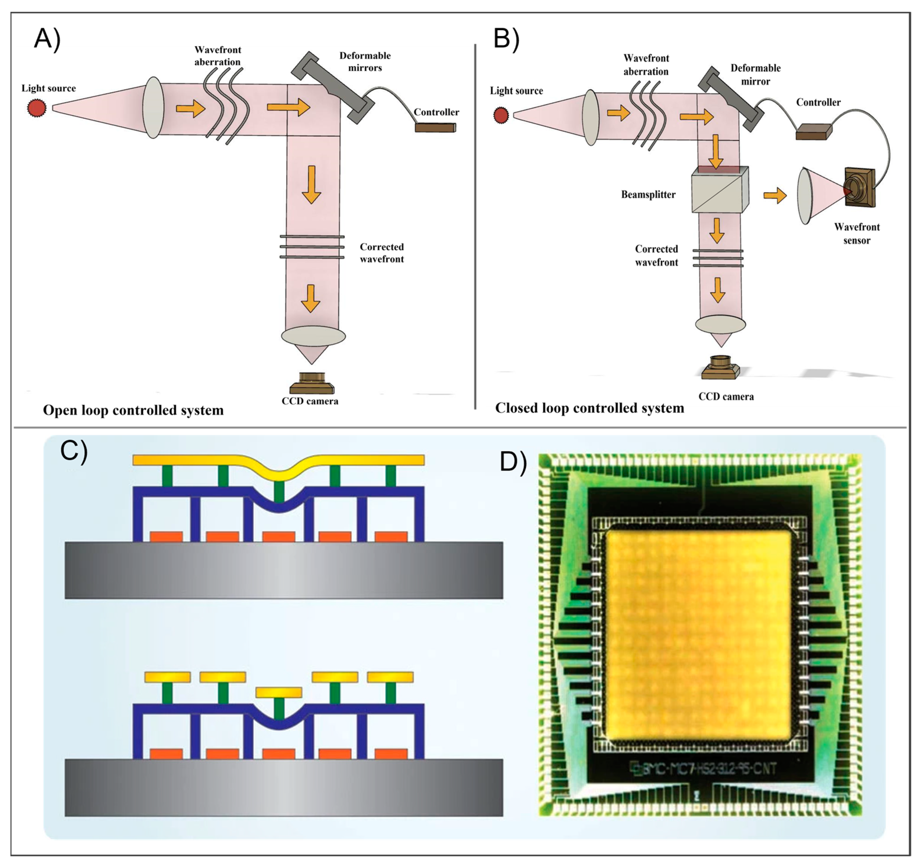
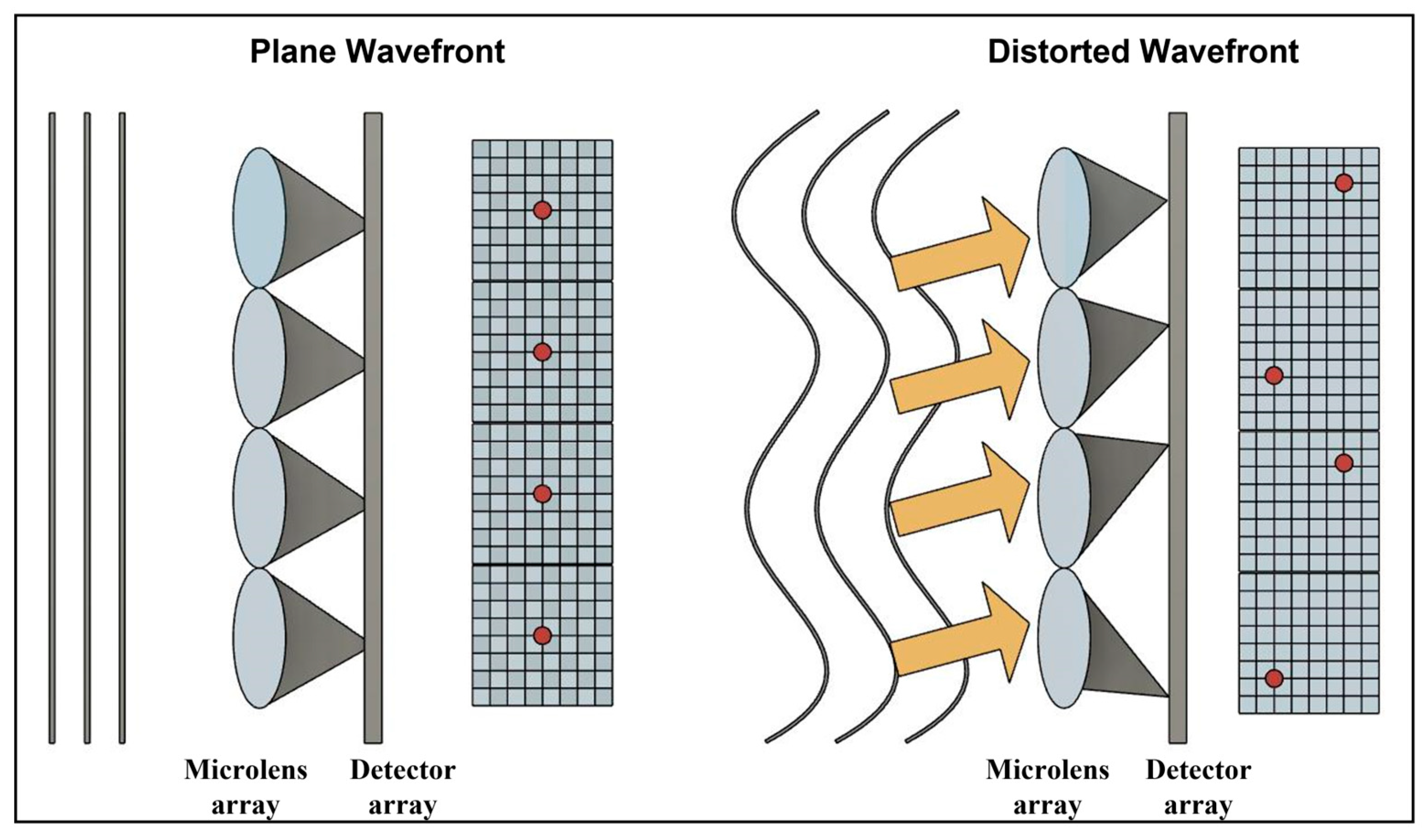
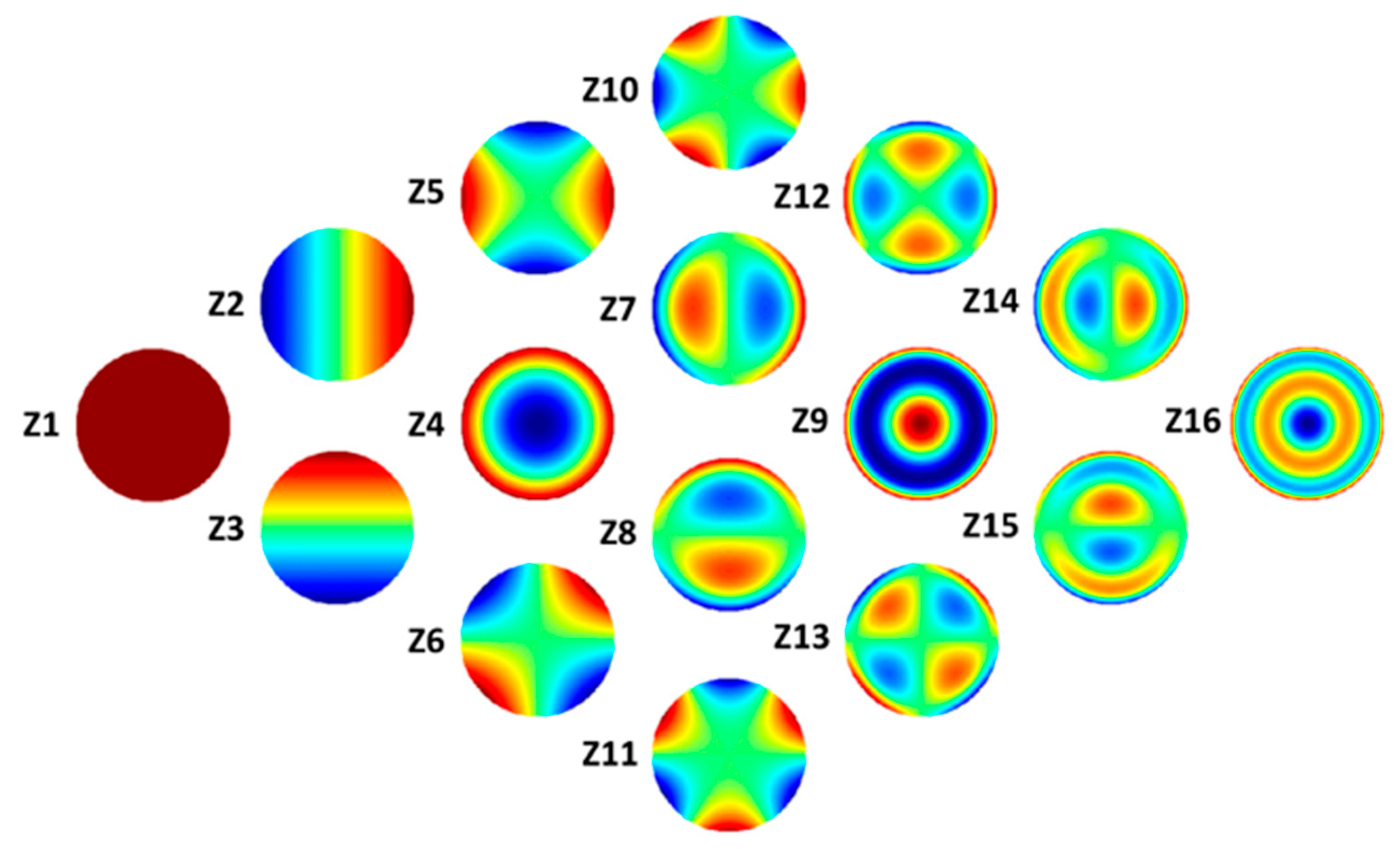
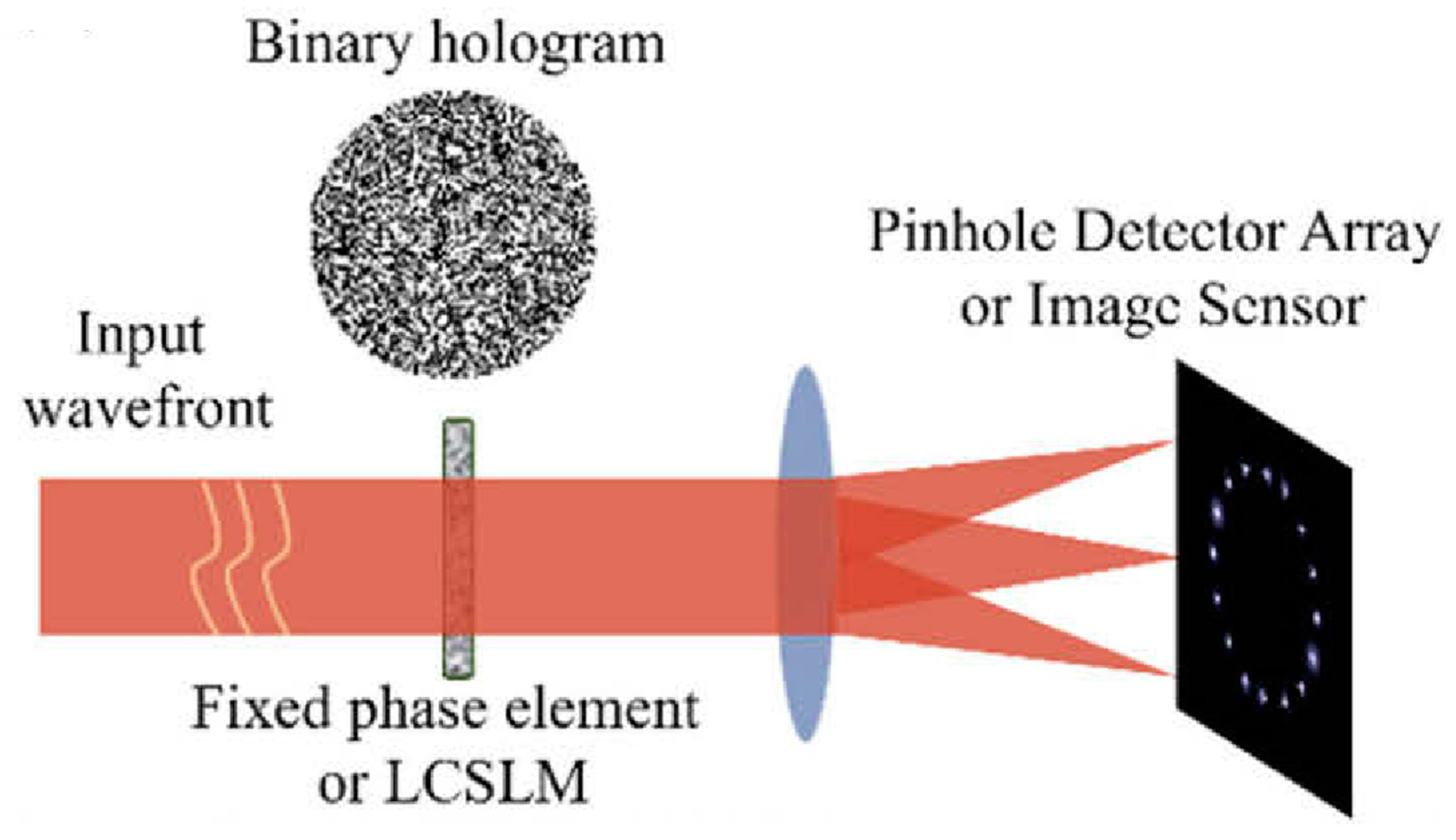
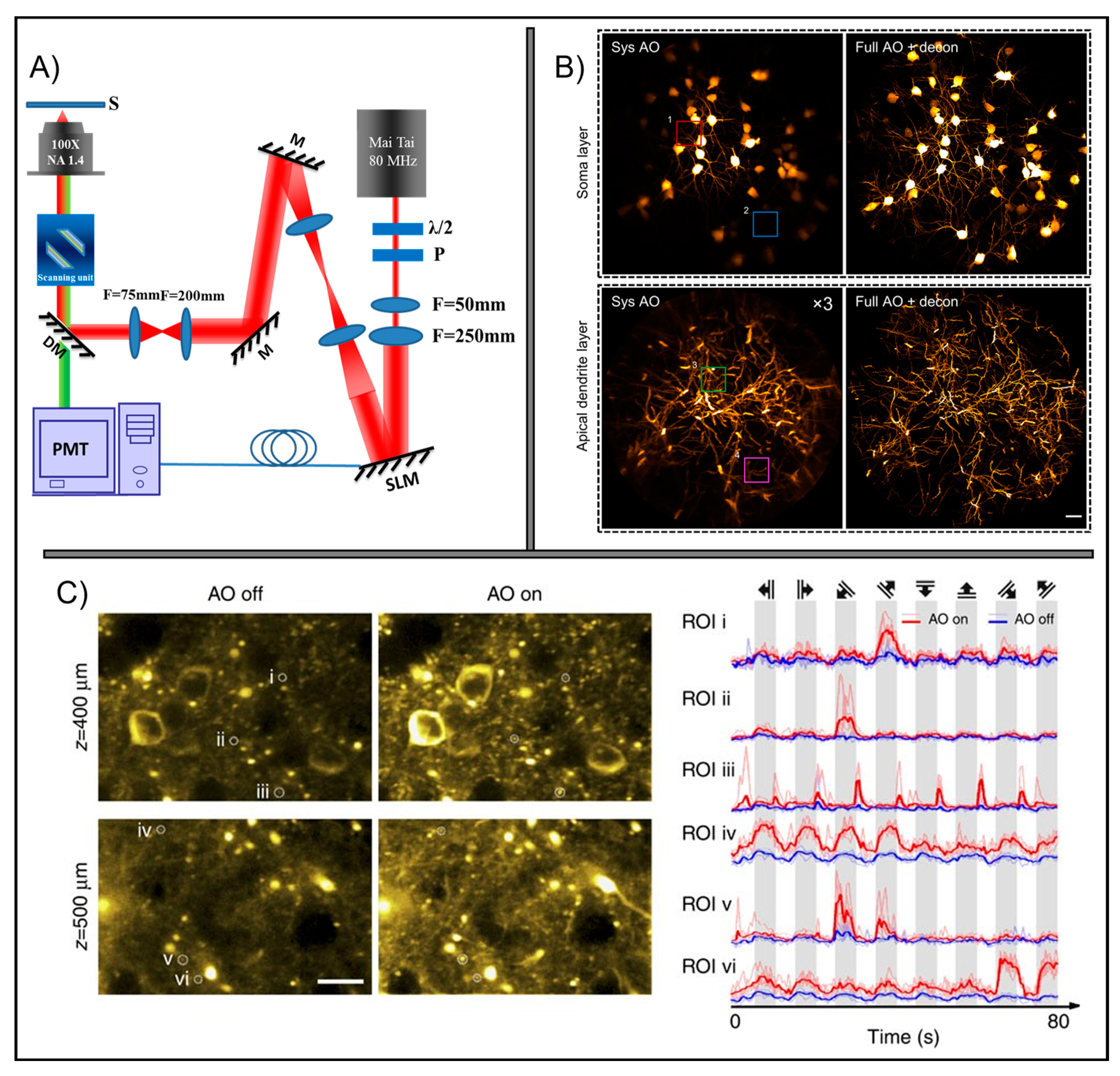
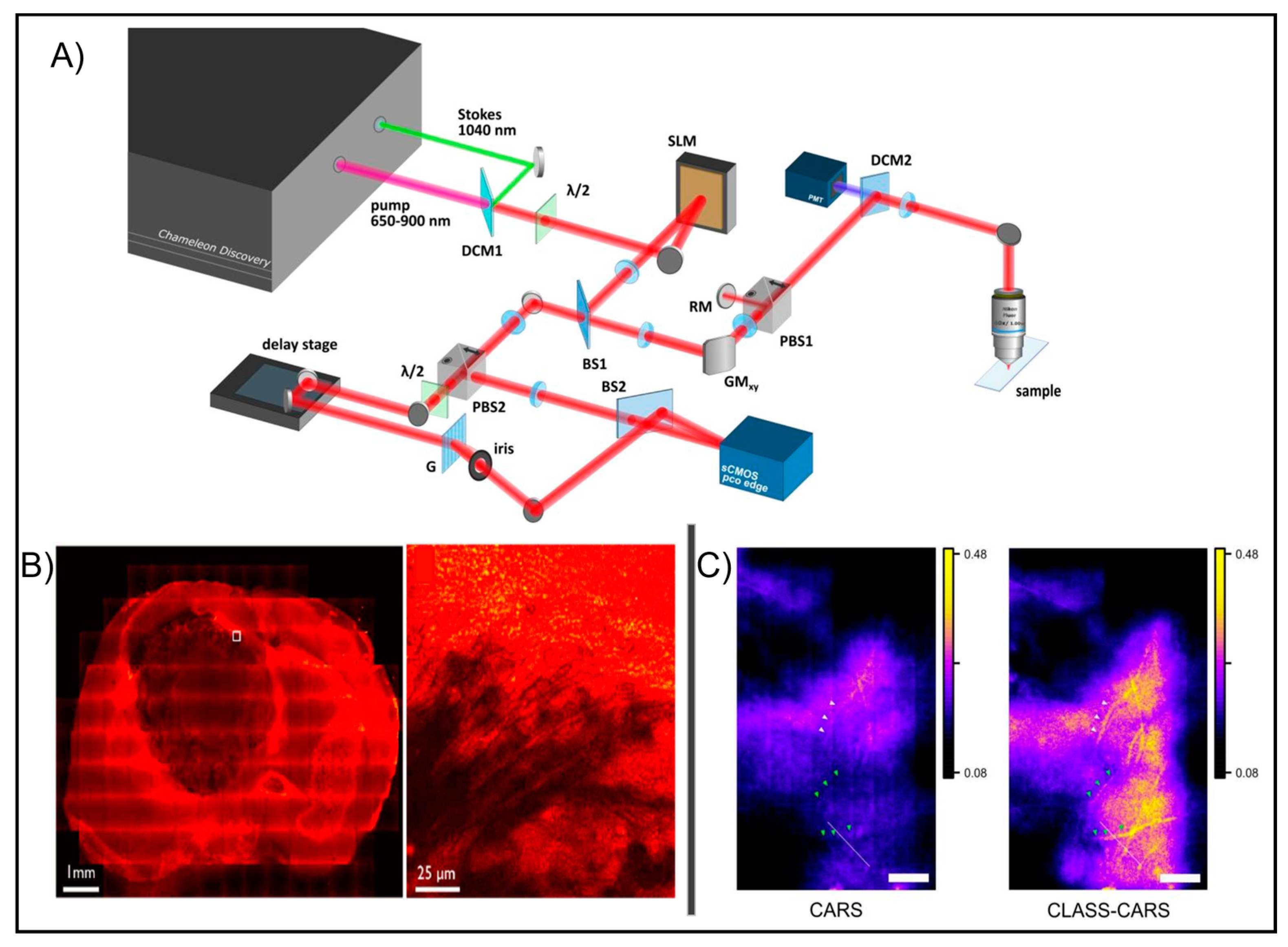
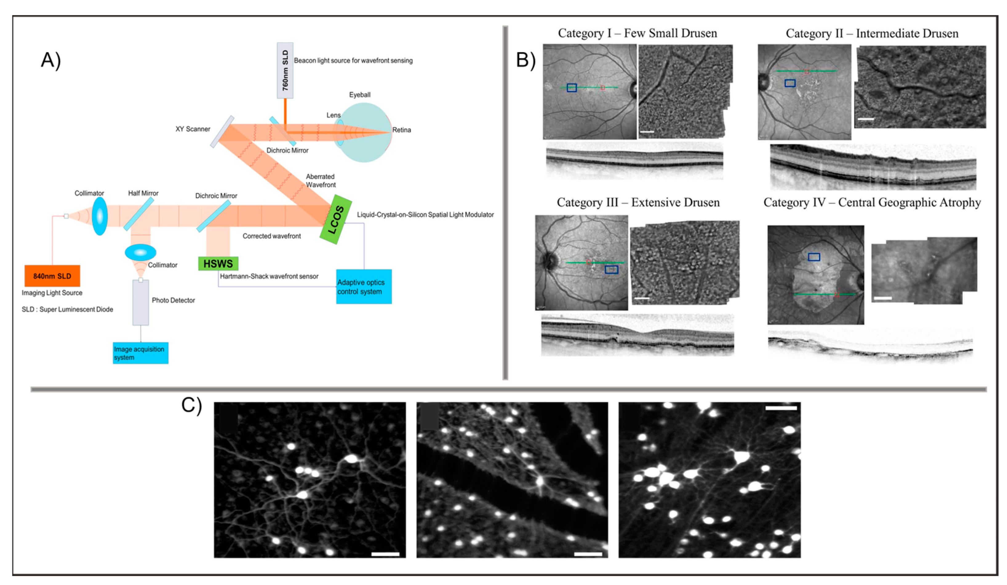
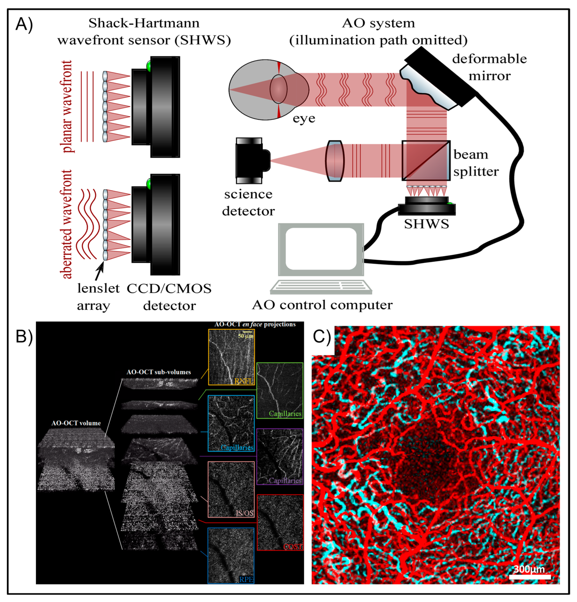
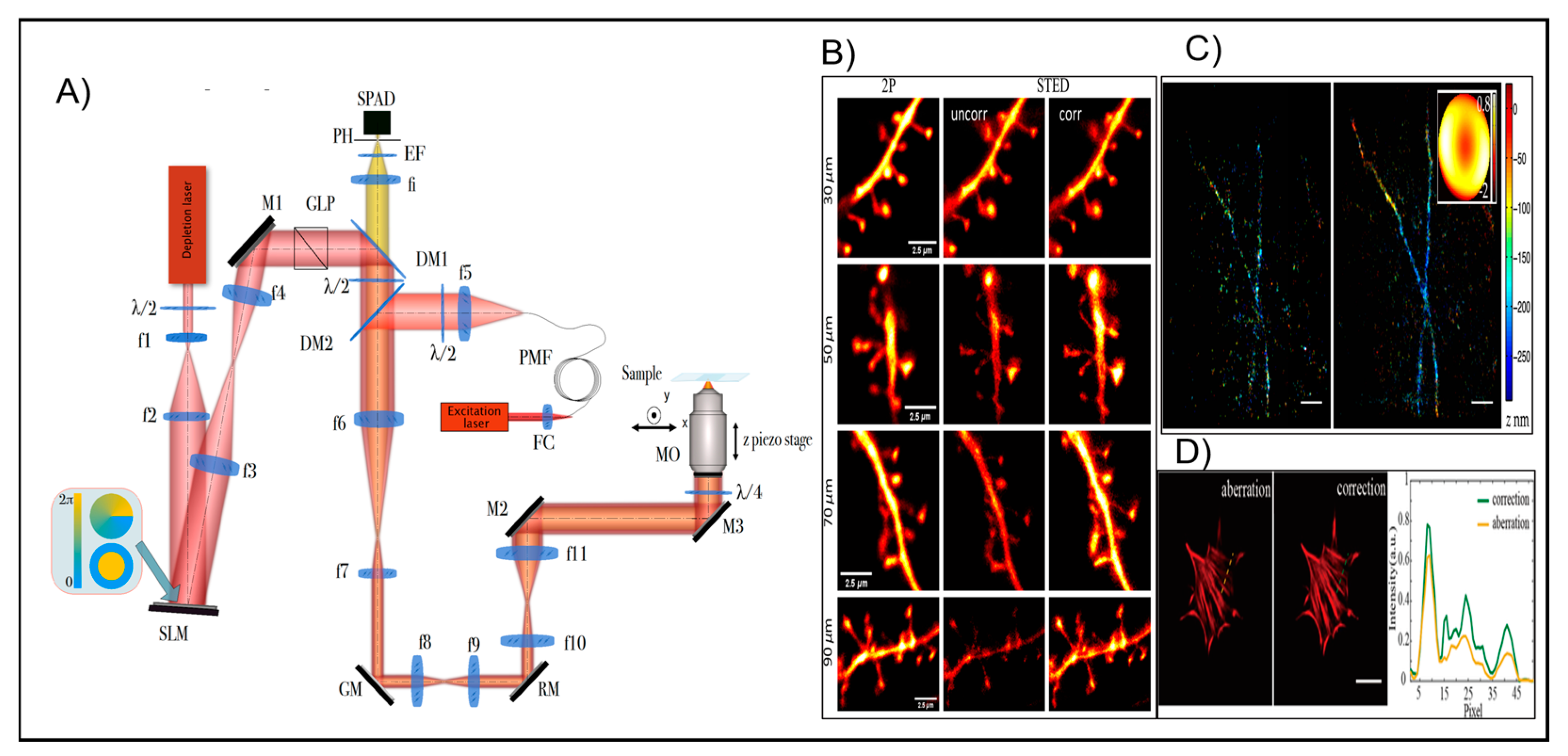
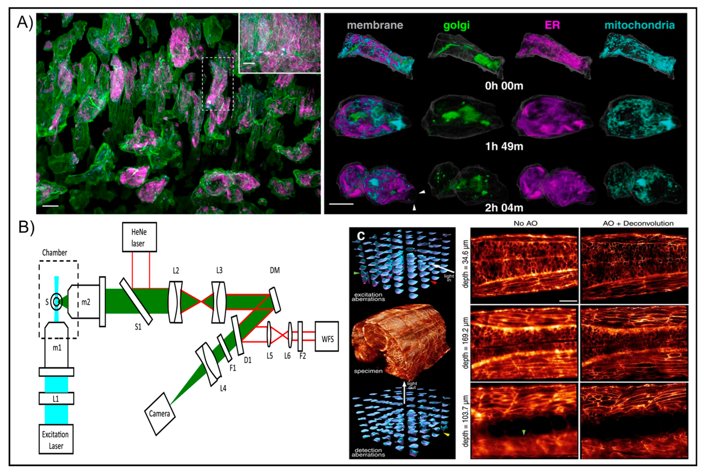
Table 1.
Comparison of the various approaches of adaptive optics.
| Approaches | Advantages | Disadvantages | References |
|---|---|---|---|
| Direct wavefront sensing | |||
| Deformable mirror, Shack–Hartmann wavefront sensor, Liquid crystal-spatial light modulator |
|
| [3,12,13,14,15,16] |
| Indirect wavefront sensing | |||
| Zonal approach and Modal approach |
|
| [7,16,17,18,19] |
Disclaimer/Publisher’s Note: The statements, opinions and data contained in all publications are solely those of the individual author(s) and contributor(s) and not of MDPI and/or the editor(s). MDPI and/or the editor(s) disclaim responsibility for any injury to people or property resulting from any ideas, methods, instructions or products referred to in the content. |
© 2023 by the authors. Licensee MDPI, Basel, Switzerland. This article is an open access article distributed under the terms and conditions of the Creative Commons Attribution (CC BY) license (https://creativecommons.org/licenses/by/4.0/).
Share and Cite
MDPI and ACS Style
Raju, G.; Mazumder, N. Digging Deeper through Biological Specimens Using Adaptive Optics-Based Optical Microscopy. Photonics 2023, 10, 178. https://doi.org/10.3390/photonics10020178
AMA Style
Raju G, Mazumder N. Digging Deeper through Biological Specimens Using Adaptive Optics-Based Optical Microscopy. Photonics. 2023; 10(2):178. https://doi.org/10.3390/photonics10020178
Chicago/Turabian StyleRaju, Gagan, and Nirmal Mazumder. 2023. "Digging Deeper through Biological Specimens Using Adaptive Optics-Based Optical Microscopy" Photonics 10, no. 2: 178. https://doi.org/10.3390/photonics10020178
Note that from the first issue of 2016, this journal uses article numbers instead of page numbers. See further details here.