
Searching for an Optimal Hexagonal Shaped Enumeration Unit Size for Effective Spatial Pattern Recognition in Choropleth Maps


Abstract
:1. Introduction
2. Related Works
2.1. The Enumeration Unit’s Role in Choropleth Map Generalization
2.2. Empirical Evaluation of Pattern Preservation on Thematic Maps
3. Materials and Methods
3.1. Materials
3.2. Study Design and Tasks
3.3. Procedure
3.4. Participants
3.5. Data Analysis
4. Results
4.1. Expected Answers
4.1.1. Map Ordering and Map Exclusion
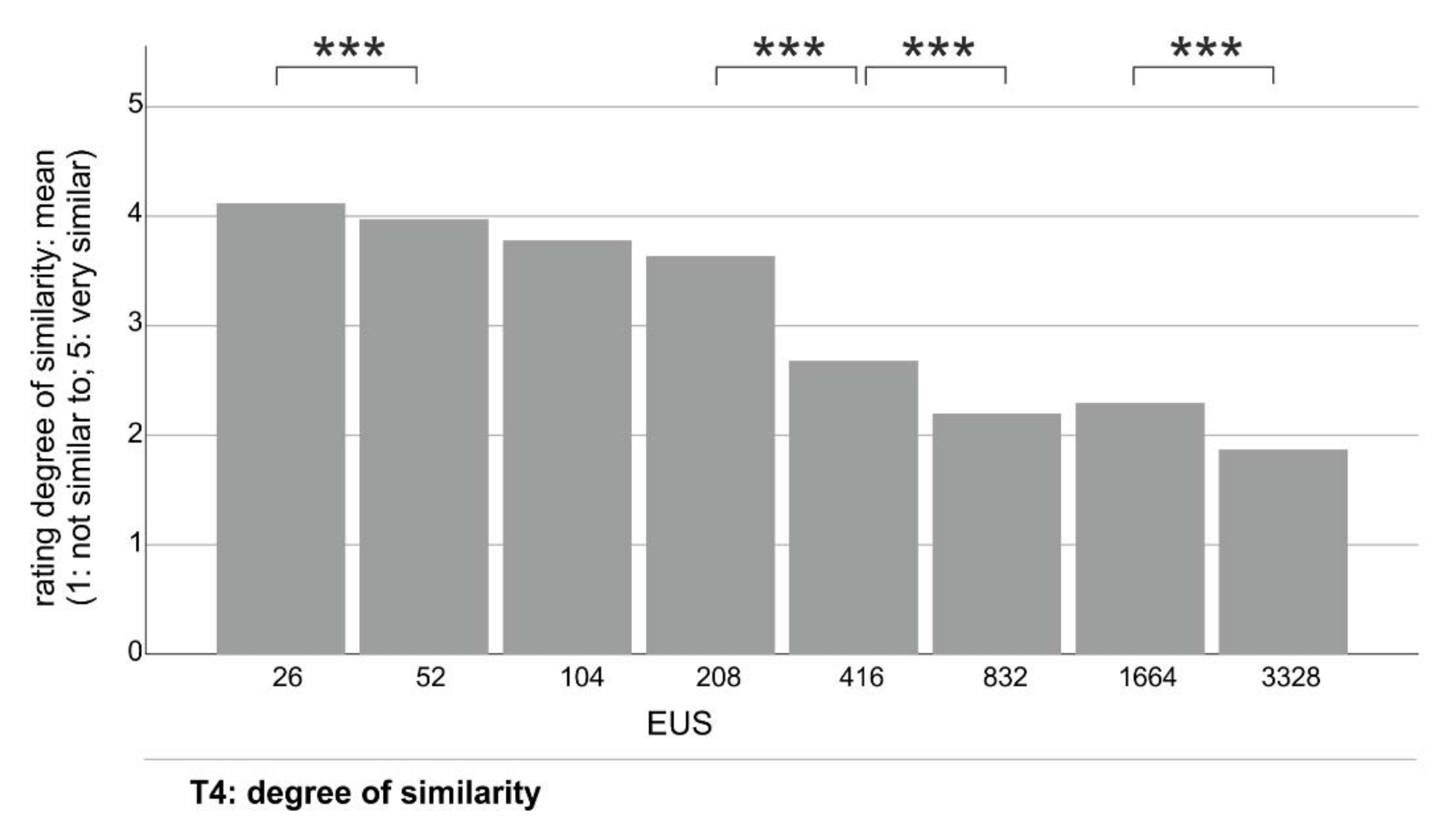
4.1.2. Perceived Usefulness and Degree of Similarity between EUS and Raw Data
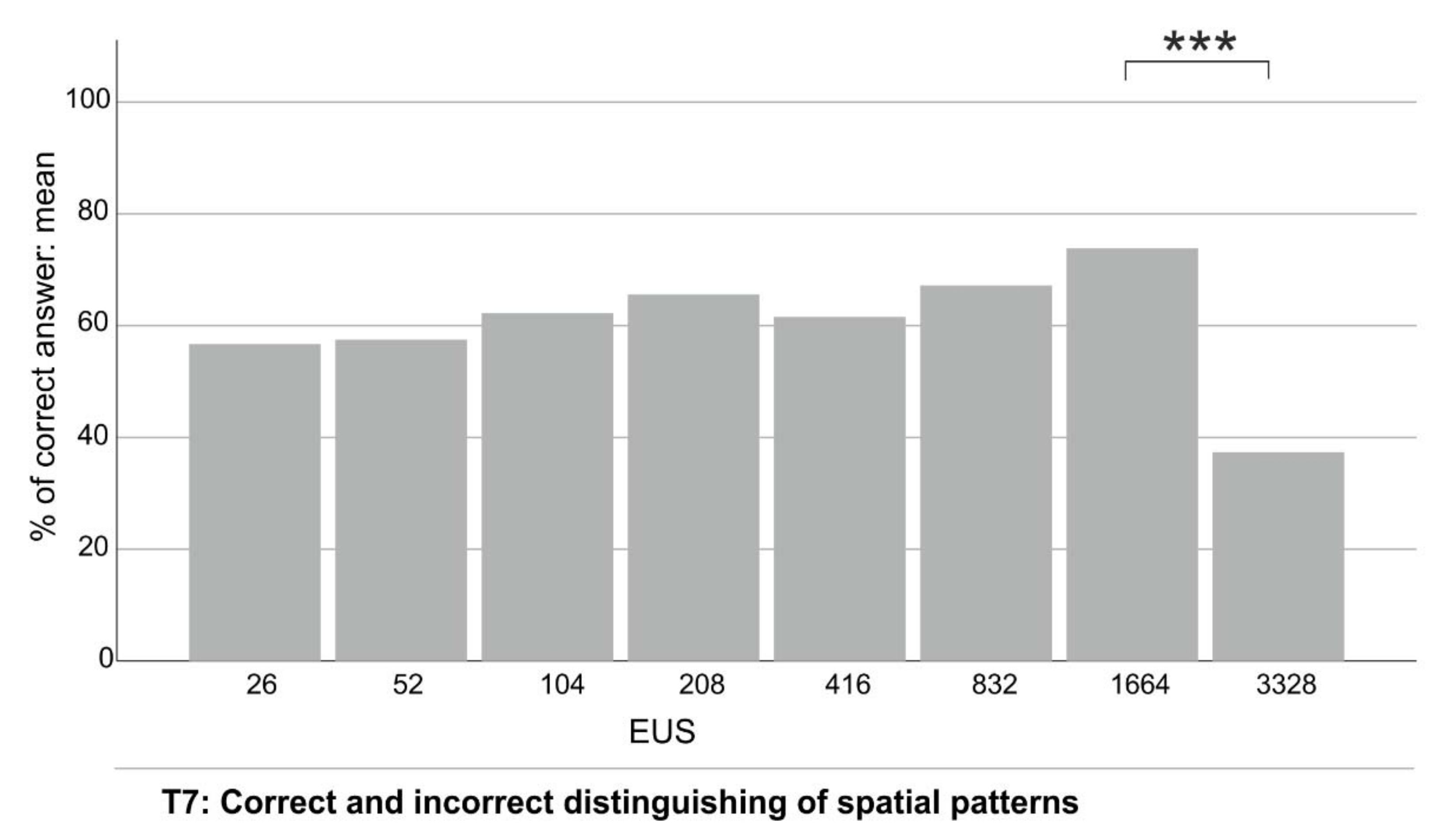
4.1.3. Spatial Pattern Recognition
4.2. Answer Times
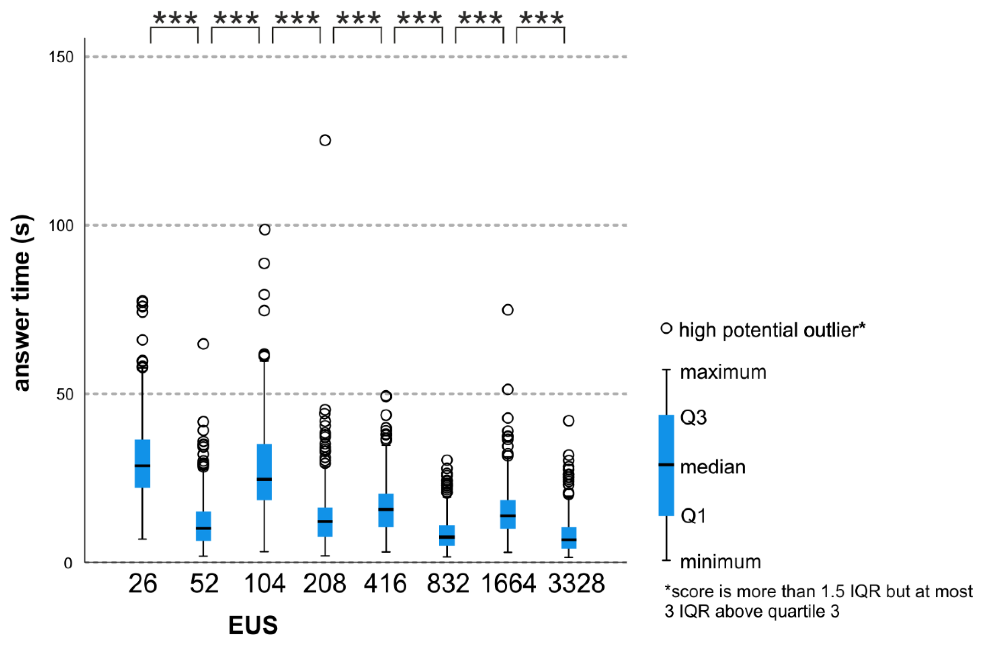
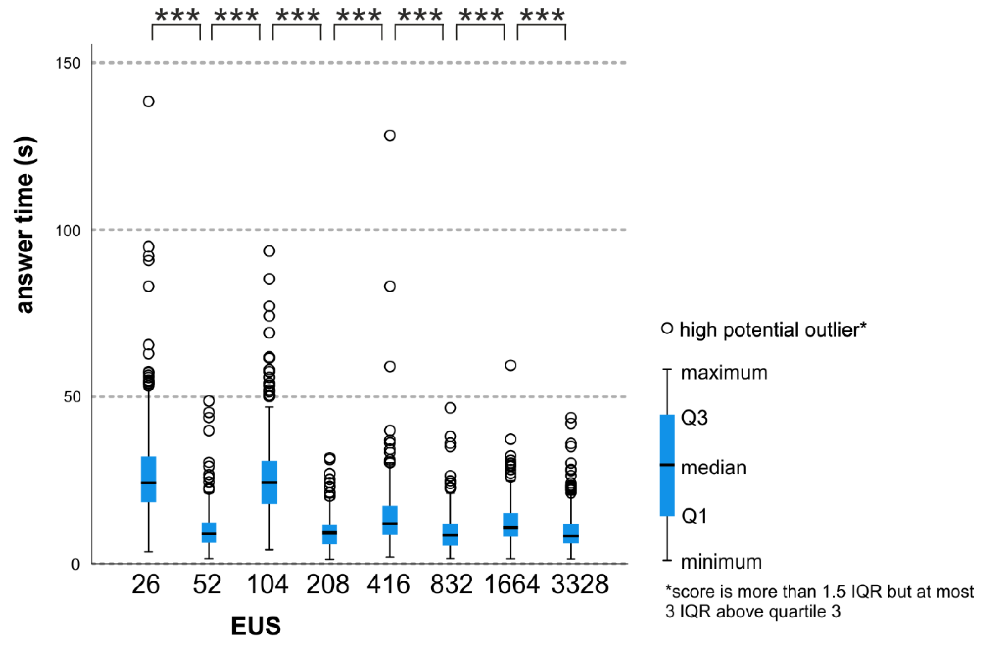
4.2.1. Usefulness and Degree of Similarity—Answer Time Comparison
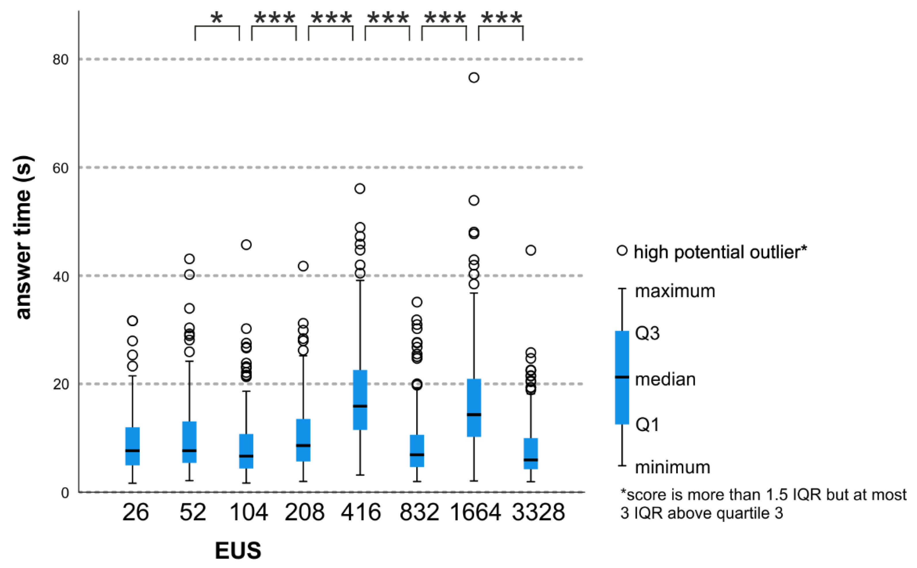
4.2.2. Spatial Pattern Recognition—Answer Time Analysis
5. Discussion
6. Conclusions
Supplementary Materials
Author Contributions
Funding
Institutional Review Board Statement
Informed Consent Statement
Data Availability Statement
Acknowledgments
Conflicts of Interest
References
- Mackaness, W.A.; Ruas, A.; Sarjakoski, L.T. Generalization of Geographic Information: Cartographic Modelling and Applications; Elsevier: Amsterdam, The Netherlands, 2007. [Google Scholar]
- Burghardt, D.; Duchêne, C.; Mackaness, W.A. Abstracting Geographic Information in a Data Rich World: Methodologies and Applications of Map Generalization; Springer International: Cham, Switzerland, 2014. [Google Scholar]
- Maceachren, A.M.; Ganter, J.H. A pattern identification approach to cartographic visualization. Cartogr. Int. J. Geogr. Inf. Geovis. 1990, 27, 64–81. [Google Scholar] [CrossRef]
- Mackaness, W.A.; Edwards, G. The importance of modelling pattern and structure in automated map generalization. In Proceedings of the Joint ISPRS/ICA Workshop on Multi-Scale Representations of Spatial Data, Ottawa, ON, Canada, 7–8 July 2002. [Google Scholar]
- Zhang, L.; Guilbert, E. Evaluation of River Network Generalization Methods for Preserving the Drainage Pattern. ISPRS Int. J. Geo. Inf. 2016, 5, 230. [Google Scholar] [CrossRef] [Green Version]
- Yu, W. Quality assessment in point feature generalization with pattern preserved. Trans. GIS 2018, 22, 872–888. [Google Scholar] [CrossRef]
- Bertin, J. Semiology of Graphics: Diagrams, Networks, Maps; University of Wisconsin Press: Madison, WI, USA, 1967. [Google Scholar]
- McMaster, R.B.; Shea, K.S. Cartographic Generalization in a Digital Environment: A Framework for Implementation in a Geographic Information System. Unkn. J. 1988, 1, 240–249. [Google Scholar]
- Brassel, K.E.; Weibel, R. A review and conceptual framework of automated map generalization. Int. J. Geogr. Inf. Syst. 1988, 2, 229–244. [Google Scholar] [CrossRef]
- Grünreich, D. Development of Computer-Assisted Generalization. In GIS and Generalization: Methodology and Practice; Müller, J.-C., Lagrange, J.-P., Weibel, R., Eds.; Taylor & Francis: London, UK, 1995; pp. 47–55. [Google Scholar]
- Dent, B.D.; Torguson, J.S.; Hodler, T.W. Cartography Thematic Map Design, 6th ed.; McGraw Hill: New York, NY, USA, 2009. [Google Scholar]
- Chang, K.-T. Data differentiation and cartographic symbolization. Cartogr. Int. J. Geogr. Inf. Geovis. 1976, 13, 60–68. [Google Scholar] [CrossRef]
- Slocum, T.A.; McMaster, R.B.; Kessler, F.C.; Howard, H.H. Thematic Cartography and Geovisualization, 3rd ed.; Pearson: Hoboken, NJ, USA, 2008. [Google Scholar]
- Cabello, S.; Haverkort, H.; Van Kreveld, M.; Speckmann, B. Algorithmic Aspects of Proportional Symbol Maps. Algorithmica 2009, 58, 543–565. [Google Scholar] [CrossRef] [Green Version]
- Schiewe, J. Empirical Studies on the Visual Perception of Spatial Patterns in Choropleth Maps. KN J. Cartogr. Geogr. Inf. 2019, 69, 217–228. [Google Scholar] [CrossRef] [Green Version]
- Hales, T.C. The Honeycomb Conjecture. Discret. Comput. Geom. 2001, 25, 1–22. [Google Scholar] [CrossRef] [Green Version]
- Montello, D.R. Cognitive Map-Design Research in the Twentieth Century: Theoretical and Empirical Approaches. Cartogr. Geogr. Inf. Sci. 2002, 29, 283–304. [Google Scholar] [CrossRef]
- MacEachren, A.M. The Role of Complexity and Symbolization Method in Thematic Map Effectiveness. Ann. Assoc. Am. Geogr. 1982, 72, 495–513. [Google Scholar] [CrossRef]
- Mersy, J.E. Trends in colour and map use research. Cartogr. Int. J. Geogr. Inf. Geovis. 1990, 27, 5–19. [Google Scholar] [CrossRef]
- Wright, J.; Robinson, A.; Sale, R.; Morrison, J. Elements of Cartography. Geogr. J. 1979, 145, 355. [Google Scholar] [CrossRef]
- Bregt, A.K.; Wopereis, M.C.S. Comparison of complexity measures for choropleth maps. Cartogr. J. 1990, 27, 85–91. [Google Scholar] [CrossRef]
- Robinson, A.H.; Morrison, J.L.; Muehrcke, P.C.; Kimerling, A.J.; Guptill, S.C. Elements of Cartography, 6th ed.; Wiley: New York, NY, USA, 1995. [Google Scholar]
- Steiniger, S.; Burghardt, D.; Weibel, R. Recognition of island structures for map generalization. In Proceedings of the 14th annual ACM international symposium on Advances in geographic information systems, Virginia, VA, USA, 10–11 November 2006; pp. 67–74. [Google Scholar]
- Touya, G.; Bucher, B.; Falquet, G.; Jaara, K.; Steiniger, S. Modelling Geographic Relationships in Automated Environments. In Lecture Notes in Geoinformation and Cartography; Cartwright, W., Gartner, G., Meng, L., Peterson, M.P., Eds.; Springer Science and Business Media LLC: Berlin, Germany, 2014; pp. 53–82. [Google Scholar]
- Sayidov, A.; Weibel, R. Constraint-based approach in geological map generalization. In Proceedings of the 19th ICA Workshop on Generalization and Multiple Representation, Helsinki, Finland, 14 July 2016. [Google Scholar]
- Boscoe, F.P.; Pickle, L.W. Choosing Geographic Units for Choropleth Rate Maps, with an Emphasis on Public Health Applications. Cartogr. Geogr. Inf. Sci. 2003, 30, 237–248. [Google Scholar] [CrossRef]
- Edsall, R.M.; Harrower, M.; Mennis, J.L. Tools for visualizing properties of spatial and temporal periodicity in geographic data. Comput. Geosci. 2000, 26, 109–118. [Google Scholar] [CrossRef] [Green Version]
- Talbot, T.O.; Kulldorff, M.; Forand, S.P.; Haley, V.B. Evaluation of spatial filters to create smoothed maps of health data. Stat. Med. 2000, 19, 2399–2408. [Google Scholar] [CrossRef]
- Openshaw, S. (Ed.) The modifiable areal unit problem. In Concepts and Techniques in Modern Geography 38; Geo Books: Norwich, UK, 1984; p. 41. [Google Scholar]
- Wong, D.W.S. The Modifiable Areal Unit Problem (MAUP). In WorldMinds: Geographical Perspectives on 100 Problems; Janelle, D.G., Warf, B., Hansen, K., Eds.; Springer Science and Business Media LLC: Berlin, Germany, 2004; pp. 571–575. [Google Scholar]
- Fotheringham, A.S.; Wong, D.W.S. The Modifiable Areal Unit Problem in Multivariate Statistical Analysis. Environ. Plan. A Econ. Space 1991, 23, 1025–1044. [Google Scholar] [CrossRef]
- Dark, S.J.; Bram, D. The modifiable areal unit problem (MAUP) in physical geography. Prog. Phys. Geogr. Earth Environ. 2007, 31, 471–479. [Google Scholar] [CrossRef] [Green Version]
- De Andrade, S.C.; Restrepo-Estrada, C.; Nunes, L.H.; Rodriguez, C.A.M.; Estrella, J.C.; Delbem, A.C.B.; de Albuquerque, J.P. A multicriteria optimization framework for the definition of the spatial granularity of urban social media analytics. Int. J. Geogr. Inf. Sci. 2021, 35, 43–62. [Google Scholar] [CrossRef]
- Cole, D.G. Recall vs. Recognition and Task Specificity in Cartographic Psychophysical Testing. Am. Cartogr. 1981, 8, 55–66. [Google Scholar] [CrossRef]
- Schiewe, J. Distortion Effects in Equal Area Unit Maps. KN J. Cartogr. Geogr. Inf. 2021, 71, 71–82. [Google Scholar] [CrossRef]
- Brewer, C.A.; MacEachren, A.M.; Pickle, L.W.; Herrmann, D. Mapping Mortality: Evaluating Color Schemes for Choropleth Maps. Ann. Assoc. Am. Geogr. 1997, 87, 411–438. [Google Scholar] [CrossRef]
- Brewer, C.A.; Pickle, L. Evaluation of Methods for Classifying Epidemiological Data on Choropleth Maps in Series. Ann. Assoc. Am. Geogr. 2002, 92, 662–681. [Google Scholar] [CrossRef]
- Lewis, D.R.; Pickle, L.W.; Zhu, L. Recent Spatiotemporal Patterns of US Lung Cancer by Histologic Type. Front. Public Health 2017, 5, 82. [Google Scholar] [CrossRef] [PubMed] [Green Version]
- Steinke, T.R.; Lloyd, R.E. Cognitive Integration of Objective Choropleth Map Attribute Information. Cartogr. Int. J. Geogr. Inf. Geovis. 1981, 18, 13–23. [Google Scholar] [CrossRef]
- Steinke, T.; Steinke, R. Judging the Similarity of Choropleth Map Images. Cartogr. Int. J. Geogr. Inf. Geovis. 1983, 20, 35–42. [Google Scholar] [CrossRef] [Green Version]
- Kraak, M.J.; Roth, R.E.; Ricker, B.; Kagawa, A.; Le Sourd, G. Mapping for a Sustainable World; The United Nations: New York, NY, USA, 2020. [Google Scholar]


| ID. Task Type | Task Question | Purpose of the Task | Maps Presented |
|---|---|---|---|
| T1. Order/rank  | The maps from A to H show, in a simplified way, the distribution of the phenomenon that is shown on map X. Arrange the maps that are labelled A to H in order from best to worst to show how well they represent the main features of the distribution of the phenomenon | Obtain feedback from the users concerning the order of the maps, in order to find the optimal EUS range. | Eight choropleth maps and the symbol map. |
T2. Distinguish/exclude | The maps from A to H show, in a simplified way, the distribution of the phenomenon that is shown on map X. Write down the letter labels ONLY OF THOSE maps that do NOT show the main features of the distribution of the phenomenon. | Examine which EUSs do not show the main characteristics of the phenomenon. | Eight choropleth maps and the symbol map. |
| T3. Compare/ Interpret  | You have been asked to indicate the main characteristics of the phenomenon presented on map X. Evaluate the suitability of map Y for this task. | Obtain feedback on users’ preferences for a particular EUS. | Map pairs: choropleth map and the symbol map. |
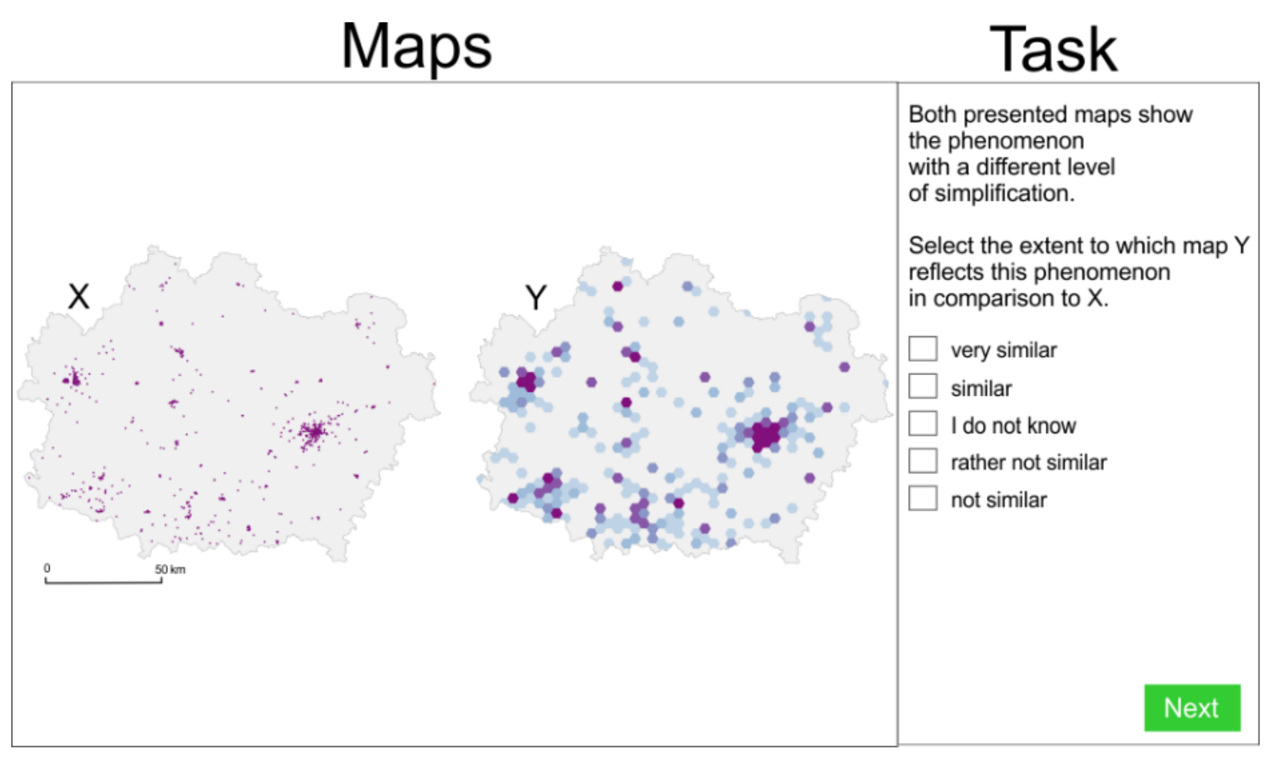
| T4. Compare/ Interpret  | Both presented maps show the phenomenon with a different level of simplification. Select the extent to which map Y reflects this phenomenon in comparison to X. | Obtain feedback on the level of similarity of the particular choropleth map to the symbol map. | Map pairs: choropleth map and the symbol map. |
| T5. Identify/draw  | Both presented maps show the phenomenon with a different level of simplification. By using the left mouse button, draw on both maps at least three corresponding areas where the phenomenon’s shape and density is similar. To finish the area, hover your mouse over the first point drawn, wait for the “paws” to appear, and then click the left mouse button. | To examine if the users can find the areas with the same shape and density on corresponding choropleth map and symbol map. | Map pairs: choropleth map and the symbol map. |
| T6. Identify/draw  | The map shows the spatial distribution of the selected phenomenon. By using the left mouse button, draw at least three lines on the map along which the phenomenon is concentrated. To end the line, double-click the left mouse button quickly. | Examine if the users can find the main axis along which the phenomenon is concentrated. | One choropleth map. |
| T7. Select  | Which of the dense areas marked on map X are visible as a similar shape on map Y. You can choose more than one answer. | Obtain information from the users as to which out of the four areas marked on the symbol map are visible on the choropleth map variant. | Map pairs: choropleth map and the symbol map. |
| Cramér’s V | p | Pairwise Comparison | Cramér’s V | p |
|---|---|---|---|---|
| 0.319 | <0.001 *** | 26–52 | 0.128 | 0.096 |
| 52–104 | 0.160 | 0.014 * | ||
| 104–208 | 0.105 | 0.243 | ||
| 208–416 | 0.258 | <0.001 *** | ||
| 416–832 | 0.304 | <0.001 *** | ||
| 832–1664 | 0.117 | 0.155 | ||
| 1664–3328 | 0.223 | <0.001 *** |
| Cramér’s V | p | Pairwise Comparison | Cramér’s V | p |
|---|---|---|---|---|
| 0.376 | <0.001 *** | 26–52 | 0.297 | <0.001 *** |
| 52–104 | 0.132 | 0.077 | ||
| 104–208 | 0.088 | 0.442 | ||
| 208–416 | 0.455 | <0.001 *** | ||
| 416–832 | 0.339 | <0.001 *** | ||
| 832–1664 | 0.107 | 0.228 | ||
| 1664–3328 | 0.286 | <0.001 *** |
| Cramér’s V | p | Pairwise Comparison | Cramér’s V | p |
|---|---|---|---|---|
| 0.109 | 0.002 ** | 26–52 | 0.004 | 0.921 |
| 52–104 | 0.026 | 0.567 | ||
| 104–208 | 0.018 | 0.696 | ||
| 208–416 | 0.022 | 0.663 | ||
| 416–832 | 0.030 | 0.500 | ||
| 832–1664 | 0.035 | 0.442 | ||
| 1664–3328 | 0.204 | <0.001 *** |
| Kruskal-Wallis H | p | Pairwise Comparison | EUS | M (s) | SD | Bonferroni Post Hoc | p |
|---|---|---|---|---|---|---|---|
| 894.730 | 0.000 *** | 26–52 | 26 | 30.76 | 12.80 | 851.701 | 0.000 *** |
| 52 | 11.98 | 8.16 | |||||
| 52–104 | 52 | 11.98 | 8.16 | −757.134 | 0.000 *** | ||
| 104 | 28.41 | 14.18 | |||||
| 104–208 | 104 | 28.41 | 14.18 | 656.095 | 0.000 *** | ||
| 208 | 13.79 | 10.84 | |||||
| 208–416 | 208 | 13.79 | 10.84 | −212.385 | 0.001 *** | ||
| 416 | 16.67 | 8.55 | |||||
| 416–832 | 416 | 16.67 | 8.55 | 518.533 | 0.000 *** | ||
| 832 | 8.86 | 5.42 | |||||
| 832–1664 | 832 | 8.86 | 5.42 | −435.960 | 0.000 *** | ||
| 1664 | 15.15 | 8.28 | |||||
| 1664–3328 | 1664 | 15.15 | 8.28 | 486.988 | 0.000 *** | ||
| 3328 | 8.36 | 6.08 |
| Kruskal-Wallis H | p | Pairwise Comparison | EUS | M (s) | SD | Bonferroni Post Hoc | p |
|---|---|---|---|---|---|---|---|
| 459.721 | 0.000 *** | 26–52 | 26 | 9.06 | 5.33 | −57.762 | 1.000 |
| 52 | 9.95 | 6.58 | |||||
| 52–104 | 52 | 9.95 | 6.58 | 170.827 | 0.025 * | ||
| 104 | 8.19 | 5.76 | |||||
| 104–208 | 104 | 8.19 | 5.76 | −213.120 | 0.001 *** | ||
| 208 | 10.28 | 6.32 | |||||
| 208–416 | 208 | 10.28 | 6.32 | −524.353 | 0.000 *** | ||
| 416 | 18.07 | 9.08 | |||||
| 416–832 | 416 | 18.07 | 9.08 | 696.988 | 0.000 *** | ||
| 832 | 8.63 | 5.94 | |||||
| 832–1664 | 832 | 8.63 | 5.94 | −595.254 | 0.000 *** | ||
| 1664 | 16.46 | 9.52 | |||||
| 1664–3328 | 1664 | 16.46 | 9.52 | 471.456 | 0.000 *** | ||
| 3328 | 7.84 | 5.45 |
| Kruskal-Wallis H | p | Pairwise Comparison | EUS | M (s) | SD | Bonferroni Post Hoc | p |
|---|---|---|---|---|---|---|---|
| 727.114 | 0.000 *** | 26–52 | 26 | 27.41 | 16.16 | 812.713 | 0.000 *** |
| 52 | 10.25 | 6.75 | |||||
| 52–104 | 52 | 10.25 | 6.75 | −813.374 | 0.000 *** | ||
| 104 | 26.37 | 13.63 | |||||
| 104–208 | 104 | 26.37 | 13.63 | 836.863 | 0.000 *** | ||
| 208 | 9.60 | 5.13 | |||||
| 208–416 | 208 | 9.60 | 5.13 | −290.803 | 0.000 *** | ||
| 416 | 14.21 | 11.42 | |||||
| 416–832 | 416 | 14.21 | 11.42 | 323.480 | 0.000 *** | ||
| 832 | 9.56 | 6.24 | |||||
| 832–1664 | 832 | 9.56 | 6.24 | −240.432 | 0.000 *** | ||
| 1664 | 12.25 | 6.86 | |||||
| 1664–3328 | 1664 | 12.25 | 6.86 | 211.973 | 0.001 *** | ||
| 3328 | 10.04 | 6.61 |
Publisher’s Note: MDPI stays neutral with regard to jurisdictional claims in published maps and institutional affiliations. |
© 2021 by the authors. Licensee MDPI, Basel, Switzerland. This article is an open access article distributed under the terms and conditions of the Creative Commons Attribution (CC BY) license (https://creativecommons.org/licenses/by/4.0/).
Share and Cite
Karsznia, I.; Gołębiowska, I.M.; Korycka-Skorupa, J.; Nowacki, T. Searching for an Optimal Hexagonal Shaped Enumeration Unit Size for Effective Spatial Pattern Recognition in Choropleth Maps. ISPRS Int. J. Geo-Inf. 2021, 10, 576. https://doi.org/10.3390/ijgi10090576
Karsznia I, Gołębiowska IM, Korycka-Skorupa J, Nowacki T. Searching for an Optimal Hexagonal Shaped Enumeration Unit Size for Effective Spatial Pattern Recognition in Choropleth Maps. ISPRS International Journal of Geo-Information. 2021; 10(9):576. https://doi.org/10.3390/ijgi10090576
Chicago/Turabian StyleKarsznia, Izabela, Izabela Małgorzata Gołębiowska, Jolanta Korycka-Skorupa, and Tomasz Nowacki. 2021. "Searching for an Optimal Hexagonal Shaped Enumeration Unit Size for Effective Spatial Pattern Recognition in Choropleth Maps" ISPRS International Journal of Geo-Information 10, no. 9: 576. https://doi.org/10.3390/ijgi10090576