
Basis Set Calculations of Heavy Atoms
by
 , , and
Mikhail G. Kozlov
1,2,*,
Yuriy A. Demidov
1,2,
Mikhail Y. Kaygorodov
1 and
Elizaveta V. Tryapitsyna
1 1
Petersburg Nuclear Physics Institute of NRC “Kurchatov Institute”, Leningrad District, Gatchina 188300, Russia
2
Department of Physics, St. Petersburg Electrotechnical University “LETI”, Prof. Popov Str. 5, St. Petersburg 197376, Russia
*
Author to whom correspondence should be addressed.
Atoms 2024, 12(1), 3; https://doi.org/10.3390/atoms12010003
Submission received: 12 December 2023
/
Revised: 5 January 2024
/
Accepted: 9 January 2024
/
Published: 12 January 2024
Abstract
:Most modern calculations of many-electron atoms use basis sets of atomic orbitals. An accurate account for electronic correlations in heavy atoms is a very difficult computational problem, and an optimization of the basis sets can reduce computational costs and increase final accuracy. Here, we propose a simple differential ansatz to form virtual orbitals from the Dirac–Fock orbitals of the core and valence electrons. We use basis sets with such orbitals to calculate different properties in Cs including hyperfine structure constants and QED corrections to the valence energies and to the transition amplitudes.
1. Introduction
Many efficient methods of atomic calculations, such as configuration interaction (CI), many-body perturbation theory (MBPT), coupled cluster (CC), or their combinations, employ basis sets of one-electron orbitals. For example, the methods CI+MBPT and CI+CC [1,2,3,4,5] use CI for valence electrons, where the electronic-correlations effects are strong, and account for weaker core-valence correlations by means of either the second order MBPT or (linearized) CC method. In these methods, the relativistic effects are treated within the no-pair approximation for the Dirac-Coulomb-Breit Hamiltonian. On the other hand, QED effects may be approximately accounted for using the model-QED-potential approach [6,7,8]. For heavy polyvalent atoms, such calculations become very computationally expensive [9]. That is why it is very important to develop efficient basis sets, which provide high accuracy at reasonable length.
The Dirac–Fock (DF) method serves as an initial approximation for most atomic calculations. In principle, the DF operator can provide us with an infinite number of eigenstates. However, in practice, it is useful to keep only some DF orbitals in the basis set. In particular, it is important to include in the basis set the entire core and some of valence orbitals. The choice of important valence orbitals depends on their occupation numbers in the atomic states we are interested in. On the other hand, the highly excited DF orbitals are usually ineffective for accounting for the correlations between valence electrons, as their radius grows too rapidly with the principal quantum number n. Because of that the B-splines [10], Sturm orbitals [11,12], or other simple orbitals [13,14] usually turn out to be more useful. Therefore, an efficient basis set has to include different types of orbitals. An effective method to merge two subsets of orbitals into one basis set was proposed in Ref. [15]. The first subset consisted of DF orbitals for the core and valence shells and the second subset consisted of B-splines, whose parameters were optimized to complement the first subset. Such mixed basis sets were tested for calculations of the valence energies of Au and Fr and sufficiently fast convergence was observed: saturation was reached for 25 splines per partial wave [15].
It is known that accurate calculations of the hyperfine structure and the parity non-conservation effects for heavy atoms are much more challenging than calculations of the energies, or transition amplitudes. These properties depend on the wave function at small distances. Correlations change the behavior of the valence-electrons wave functions in this region and lead to large corrections to the matrix elements of these operators. Because of that the convergence with respect to the number of orbitals in the basis set is typically much slower. Test calculations of the magnetic hyperfine constant A for Au did not converge even for the mixed basis set with 45 B-splines per partial wave [15]. It was found that the small components of the valence orbitals near the origin were not smooth. Increasing the size of the basis set decreased the amplitude of these non-physical dips or bumps, but shifted them closer to the origin, where the hyperfine interaction was particularly strong. The solution proposed in that paper was to add to the basis set a small number of DF orbitals for the ion AuM+, or, in other words, the orbitals for the potential, where N is the number of electrons in the neutral atom. Such orbitals are similar to those of the neutral atom, but are more contracted. That allowed to smoothly change the orbitals near the nucleus. After that the calculation of the hyperfine constants A for Au already converged for two such ionic orbitals and 24 B-splines per partial wave. For this recipe to work one needs to choose M in such a way that ionic orbitals are neither too different, nor too similar to those of the neutral atom. In the former case, such orbitals become less useful, while in the latter one can run into the linear dependency problem. In Ref. [15] the orbitals for the potential were used. Here, we propose another method to form additional orbitals to supplement DF orbitals and B-splines. The new procedure is more formal and does not require arbitrary adjustments. We test these basis sets for calculation of the QED corrections and hyperfine constants in neutral Cs.
2. Method
The basis set for atomic calculations consists of subsets for different partial waves, which are defined by the relativistic quantum number , where l and j are the orbital and total angular momenta. The relativistic two-component radial wave functions have the form
Most atomic calculations are done in the no-pair approximation [16,17,18], when the Dirac–Coulomb, or Dirac–Coulomb–Breit Hamiltonian is projected on the positive-energy states of the one-electron Dirac operator. Within this approximation the QED corrections can be included approximately by means of the model operators [7,8,19]. The exact form of the projection operator to the positive energy states is unknown, and some additional approximation has to be used. The most common method to exclude negative energy continuum from the basis set is to imply the kinetic balance condition [20] on the lower components of the basis orbitals, Equation (1):
where is the fine structure constant (if not stated otherwise, we use atomic units throughout the paper). Let us mention that for the ab initio atomic QED calculations beyond the no-pair approximation the basis sets are usually formed with the help of the dual kinetic balance method [21]. Such basis sets accurately approximate negative continuum of the Dirac spectrum. In this paper we neglect all contributions from the negative continuum. Therefore, below we assume that the small components are always formed with the help of Equation (2) and focus on the large components P.
When some small perturbation is added to the Hamiltonian, the large component P of the electronic orbital changes slightly. These changes do not affect the asymptotic behavior at large and small distances and the number of nodes of the function P remains the same. To account for such changes we need to add basis functions with similar features. Let us consider a simple stretching transformation:
where , . Expanding in powers of we get:
Thus, if we want to guarantee that the stretched DF orbital can be accurately expanded in the basis set, we can add a virtual orbital:
where index v numerates virtual orbitals for a partial wave with the given relativistic quantum number . Note that this function has the same asymptotic behavior for and for as , however it has an extra node. When new orbital is added to the basis set, we first generate the small component using the kinetic balance condition, Equation (2), then we orthogonalize it to all the other orbitals with the same quantum number and normalize it to unity. The index v here does not mean principal quantum number and is not linked to the number of nodes, which changes during the orthogonalization process. Only if we diagonalize the Hamiltonian matrix on the basis set, the new eigenvectors can be indexed with the principal quantum number n.
3. Test Calculations for Cs
To illustrate usefulness of the ansatz from Equation (5) let us consider QED corrections in neutral Cs. Firstly, we used a sufficiently large basis set to diagonalize the Dirac-Fock operator together with the model QED potential from Refs. [19,22]. After that, we calculated the difference between the large components with and without QED corrections and compared them with the respective scaled orbitals from Equation (5). Figure 1 shows that the latter very much resemble the former. Thus, we can expect that adding orbitals generated with the help of Equation (5) to the basis set will significantly improve its quality and will speed up the convergence.
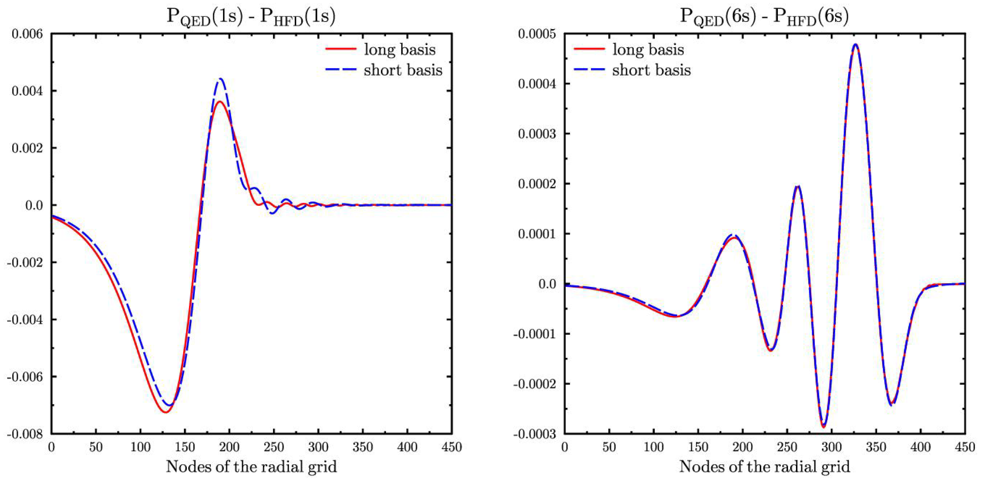
We formed the basis set for Cs which included DF orbitals , , and , where . For each DF orbital we added respective virtual orbital using the differential ansatz. To ensure that the number of virtual orbitals is the same in each partial wave, we formed one additional p orbital per partial wave and three additional d orbitals per partial wave using the method of Ref. [14]. Thus, this basis set included seven virtual orbitals per partial wave, or sixty-two orbitals in total. This calculation was compared with calculation performed using the long basis set, which included these seven virtual orbitals plus twenty-three additional ones per partial wave. Below, we refer to these basis sets as B7 and B30, respectively. Figure 2 shows the difference between the perturbed by the model QED operator and orbitals for Cs and unperturbed ones. We see that the QED correction for the orbital has some non-physical oscillations in both basis sets, but their amplitude for the large basis set is few times smaller. Such oscillations are typical for the calculations with finite basis sets and they indicate that convergence is not yet achieved. For the valence orbital the QED correction is practically the same for both basis sets, which means that the convergence here is reached already for the short basis set. Similar situation is observed for the valence orbitals.
In the calculations of neutral atoms one usually explicitly need to know only the wave functions of the valence electrons, where the short basis set seems to work nicely. To test it further, we calculated QED corrections to the valence binding energies and to the E1 transition amplitudes. In both cases we used the model QED potential [19]. This model potential accounts for the QED corrections to the wave functions. For the E1 amplitudes there are also QED corrections to the vertex, which are not included here. They were calculated in Refs. [23,24] and found to be much smaller than the corrections to the wave functions. Results obtained with the basis sets B7 and B30 are compared in Table 1. We see that two calculations give practically identical QED correction to the binding energy of the electron. For the other partial waves, the corrections to the energies are much smaller and the difference between results is about 1–2% (the absolute difference is of the same order of magnitude, as for the s wave). For the s–p transition amplitudes the agreement is again very good, but for the p–d transitions the difference between the two basis sets is about 10%. On the one hand, these corrections are small. On the other hand, in the d wave we have only four orbitals formed with the help of the differential ansatz, while other three orbitals of the basis set B7 are apparently less useful. This is the reason why the short basis set for the d wave is not as efficient, as for the case of s and p waves.
We mentioned earlier that convergence in calculations of the hyperfine constants A is often very slow. Because of that we compared the random-phase approximation (RPA) corrections for these constants obtained with the basis sets B7 and B30. For the orbitals , , and the difference was around 1% of the RPA correction. Note that this corresponds to a fraction of a percent in respect to the final value of the hyperfine constant. This is smaller, than, for example, the Bohr-Weisskopf, or the Breit-Rosenthal corrections (the former is caused by the distributions of magnetization inside the nucleus and the latter is associated with the nuclear charge distribution). Our final values of the RPA corrections to the constants GHz and are close to the values obtained in Ref. Dzuba et al. [25], 289 GHz and 39 GHz, respectively.
Results presented in Table 2 show that the basis sets, which include virtual orbitals, generated with the help of Equation (5), provide fast convergence for calculations of the QED and RPA corrections, which are particularly sensitive to the quality of the basis set. Below we compare QED corrections calculated with these basis sets with the values reported in the literature by other groups and study potential sources of the differences. We focus primarily on the QED corrections to the transition amplitudes.
3.1. QED Corrections to the E1 Amplitudes in Cs
There are many calculations of the QED corrections to the transition amplitudes in highly-charged ions, see for example [23,26,27]. However, for neutral atoms and weakly charged ions, these corrections are usually neglected. The most prominent exception is neutral Cs, where QED corrections to the amplitudes were calculated several times. Sapirstein and Cheng [24] calculated amplitude within the one-determinant approximation, while calculations [28,29,30] included correlations, but neglected the vertex correction. Traditionally QED corrections to the amplitude are expressed in terms of the parameter R:
where is the amplitude without QED correction. There are two contributions to the QED correction R:
where accounts for the correction to the one-electron wave functions (perturbed orbitals) and is the vertex correction. The former is supposed to be larger than the latter [7] and it can be approximately calculated with the help of the model QED potentials. At present, the effective operator for the vertex correction is unknown, and it can be calculated only within the consistent QED approach.
In Table 2 we compare our results for with results of other groups. Sapirstein and Cheng [24] made ab initio QED calculation using the local Kohn-Sham potential. They calculated both corrections and found, that the vertex correction was significantly smaller, . Other calculations used the non-local DF operator and the model potential [7,31,32]. Here we made calculations with model potentials [7,19], which we denote as STY and FG potentials, respectively.

Table 2.
Comparison of the PO QED corrections (see Equation (7)) to the transition amplitudes in Cs with other calculations. Our calculations were done using the model potentials STY [19] and FG [7].
| Transition | This Work | [24] | [28] | [29] | |
|---|---|---|---|---|---|
| Method | STY | FG | Ab Initio (KS) | FG | FG |
| 0.262 | 0.267 | 0.326 | 0.272 | 0.26 | |
| 0.275 | 0.280 | 0.286 | 0.28 | ||
| −2.89 | −2.97 | −2.80 | −2.89 | ||
| −1.84 | −1.84 | −1.76 | −1.84 | ||
| −0.442 | −0.452 | −0.433 | −0.44 | ||
| −0.369 | −0.376 | −0.359 | −0.37 | ||
Table 2 shows that the results obtained with two QED potentials agree within 2–3%. The difference between different groups is somewhat bigger, about 4–6%. There are small differences in the model potentials described in Refs. [7,31,32]. Incompleteness of the basis sets can be another reasons of the disagreements. The only direct QED calculation is about 20% larger, than all three calculations with the model potentials. Note that this calculation was done with the local Kohn-Sham potential instead of the non-local DF potential used by all other groups. Because of that, it is important to check, how much QED corrections to the E1 amplitudes depend on the choice of the potential. Note also that the parametrization in Equation (6) allows one to partly compensate for differences in the value of the initial amplitude in different approximations.
3.2. Local Screening Potentials
We made calculations with the model QED operator [19] and three widely used local screening potentials: the first one is the core-Hartree potential (CH) induced by the core electrons of Cs+ ground-state configuration, the other two are the Kohn-Sham (KS) [33] and Slater (S) [34] potentials corresponding to the ground-state configuration of the neutral Cs. The proper asymptotic behavior of the potentials KS and S is restored by including the Latter correction [35]. In Table 3 the results obtained using these three local screening potentials are compared with the Dirac-Fock results. We see that calculations of QED corrections with local potentials do not correlate with the DF calculations for all partial waves, but the s wave. The reason for this discrepancy is obvious. In the DF approximation the energy correction comes from the direct contribution of the perturbation and the contribution from the adjustment of the self-consistent field (relaxation of the core) . The former is large for the s wave and rapidly decreases with the orbital quantum number l. At the same time, the relaxation of the core similarly affects all valence orbitals. Two contributions become comparable already for the valence p orbitals. For the local potentials there is only the direct contribution. The KS potential reproduces valence orbital energies better than two other potentials. The average deviation from the DF values is about 3% for the KS potential, and 6% and 9% for the CH and S potentials, respectively. QED corrections to the s wave energies for the CH and KS potentials are of the similar accuracy, 6% and 8% respectively, while for S potential the errors are almost 50%. Slater screening potential is clearly the least accurate.
Taking into account that the core relaxation is very important for the p and d waves, the local approximation is clearly inapplicable for the QED corrections to the transitions between p and d orbitals. The results of the calculations for the transitions are presented in Table 4. Again, the KS potential gives better agreement with the DF method, than two other potentials. In most cases the difference is less, or about 10%. The only exception is the transition, where the difference is 24%. For the CH and S potentials the average differences are about 14% and 22%, respectively.
We conclude that for Cs the KS potential provides higher accuracy for the QED calculations than CH and S potentials. It should be noted, that the result of Sapirstein and Cheng [24] for the transition cited in Table 2 was obtained using KS potential. Our KS value is closer to their value, than the DF one. Thus, the approximately 20% difference between ab initio calculation [24] and calculations with model QED potentials presented in Table 2 can be attributed in part to the local potential error. This once again demonstrate the importance and usefulness of the model QED potentials for the calculations of the QED corrections in multielectron atoms.
4. Conclusions
Many numerical methods for atomic calculations require one-electron basis sets. Here we proposed the differential ansatz to generate virtual orbitals from the DF orbitals of the core and valence electrons. The number of such orbitals cannot exceed the number of DF orbitals. More virtual orbitals can be added using B-splines, or other traditional methods. Our test calculations for Cs showed good convergence of calculations of different properties, including QED corrections and hyperfine structure constants.
Another possible application of our differential ansatz may be for the multiconfigurational calculations of the complex polyvalent atoms. The size of the configuration space roughly scales as , where M is the number of correlated electrons and N is the number of valence and virtual orbitals in the basis set. That puts a very stringent limit on the permissible length of the basis set for . Thus, we expect that adding virtual orbitals generated with the help of Equation (5) from the outer-core and the valence DF orbitals will be useful for treating valence correlations in such systems. In particular, it is known, that changing of the occupation number of the valence d shell of a transition metal, or the valence f shell of a rare earth metal, leads to the relaxation of the whole respective shell. To a first approximation, this relaxation can be described by the stretching transformation, given by Equation (3). Therefore, adding a single virtual orbital, Equation (5), can describe most of this relaxation. We plan to report results of such calculations in the near future.
We also tested three local potentials, which are often used for the QED calculations in many-electron atoms and found out that for the lowest partial wave the Kohn-Sham local potential demonstrated the best agreement with the DF potential. For the higher partial waves, the results obtained with all tested local potentials are very different from the results obtained with the non-local DF potential. These differences are caused by the absences of the contribution from the change of the self-consistent field induced by the perturbation. This effect becomes dominant for the partial waves with making calculation of the respective QED corrections problematic. In order to improve the accuracy of the ab initio QED calculations in heavy atoms, it is necessary to include core-relaxation effects by going to the next order of the perturbation theory in the electron-electron interaction. At present, the quantum-mechanical approach allows for more accurate treatment of electronic correlations. In this approachl, the QED corrections can be included by means of the effective, or model QED operators. Existing model QED potentials allow one to account for the corrections to the electronic binding energies and the so-called ’perturbed orbital’ corrections to the transition amplitudes. On the next step, it is necessary to construct effective QED operators to account for the currently neglected vertex contributions.
Author Contributions
Conceptualization and methodology M.G.K., Y.A.D. and M.Y.K.; calculations M.G.K., Y.A.D., M.Y.K. and E.V.T.; writing—original draft preparation, M.G.K.; writing—review and editing, M.G.K., Y.A.D., M.Y.K. and E.V.T. All authors have read and agreed to the published version of the manuscript.
Funding
This work was supported by the Russian Science Foundation grant #23-22-00079.
Data Availability Statement
The data in this article is the results of the authors’ computer calculations. The data presented in this study are available on request from the corresponding author.
Acknowledgments
We are grateful to Ilya Tupitsyn and Vladimir Yerokhin for extremely useful discussions and suggestions.
Conflicts of Interest
The authors declare no conflicts of interest.
References
- Dzuba, V.A.; Flambaum, V.V.; Kozlov, M.G. Combination of the many-body perturbation theory with the configuration-interaction method. Phys. Rev. A 1996, 54, 3948–3959. [Google Scholar] [CrossRef] [PubMed]
- Kozlov, M.G. Precision calculations of atoms with few valence electrons. Int. J. Quant. Chem. 2004, 100, 336. [Google Scholar] [CrossRef]
- Dzuba, V.A. VN − M approximation for atomic calculations. Phys. Rev. A 2005, 71, 032512. [Google Scholar] [CrossRef]
- Safronova, M.S.; Kozlov, M.G.; Johnson, W.R.; Jiang, D. Development of a configuration-interaction + all-order method for atomic calculations. Phys. Rev. A 2009, 80, 012516. [Google Scholar] [CrossRef]
- Kahl, E.; Berengut, J. ambit: A programme for high-precision relativistic atomic structure calculations. Comput. Phys. Commun. 2019, 238, 232–243. [Google Scholar] [CrossRef]
- Pyykkö, P.; Zhao, L.B. Search for Effective Local Model Potentials for Simulation of Quantum Electrodynamic Effects in Relativistic Calculations. J. Phys. B At. Mol. Opt. Phys. 2003, 36, 1469–1478. [Google Scholar] [CrossRef]
- Flambaum, V.V.; Ginges, J.S.M. Radiative potential and calculations of QED radiative corrections to energy levels and electromagnetic amplitudes in many-electron atoms. Phys. Rev. A 2005, 72, 052115. [Google Scholar] [CrossRef]
- Tupitsyn, I.I.; Berseneva, E.V. A Single-Particle Nonlocal Potential for Taking into Account Quantum-Electrodynamic Corrections in Calculations of the Electronic Structure of Atoms. Opt. Spectrosc. 2013, 114, 682. [Google Scholar] [CrossRef]
- Cheung, C.; Safronova, M.; Porsev, S. Scalable Codes for Precision Calculations of Properties of Complex Atomic Systems. Symmetry 2021, 13, 621. [Google Scholar] [CrossRef]
- Johnson, W.R.; Blundell, S.A.; Sapirstein, J. Finite basis sets for the Dirac equation constructed from B-splines. Phys. Rev. A 1988, 37, 307. [Google Scholar] [CrossRef]
- Tupitsyn, I.I.; Loginov, A.V. Use of sturmian expansions in calculations of the hyperfine structure of atomic spectra. Opt. Spectrosc. 2003, 94, 319–326. [Google Scholar] [CrossRef]
- Kotochigova, S.; Kirby, K.P.; Tupitsyn, I. Ab initio fully relativistic calculations of x-ray spectra of highly charged ions. Phys. Rev. A 2007, 76, 052513. [Google Scholar] [CrossRef]
- Bogdanovich, P.; Žukauskas, G. The simplified superposition of configurations in the atomic spectra. Sov. Phys. Collect. 1983, 23, 18–33. [Google Scholar]
- Kozlov, M.G.; Porsev, S.G.; Flambaum, V.V. Manifestation of the Nuclear Anapole Moment in the M1 Transitions in Bismuth. J. Phys. B 1996, 29, 689–697. [Google Scholar] [CrossRef]
- Kozlov, M.; Tupitsyn, I. Mixed Basis Sets for Atomic Calculations. Atoms 2019, 7, 92. [Google Scholar] [CrossRef]
- Faustov, R.N. Quasipotential Method in the Bound State Problem. Theor. Math. Phys. 1970, 3, 478–488. [Google Scholar] [CrossRef]
- Sucher, J. Foundations of the Relativistic Theory of Many-Electron Atoms. Phys. Rev. A 1980, 22, 348. [Google Scholar] [CrossRef]
- Mittleman, M.H. Theory of Relativistic Effects on Atoms: Configuration-space Hamiltonian. Phys. Rev. A 1981, 24, 1167. [Google Scholar] [CrossRef]
- Shabaev, V.M.; Tupitsyn, I.I.; Yerokhin, V.A. Model operator approach to the Lamb shift calculations in relativistic many-electron atoms. Phys. Rev. A 2013, 88, 012513. [Google Scholar] [CrossRef]
- Stanton, R.E.; Havriliak, S. Kinetic balance: A partial solution to the problem of variational safety in Dirac calculations. J. Chem. Phys. 1984, 81, 1910–1918. [Google Scholar] [CrossRef]
- Shabaev, V.M.; Tupitsyn, I.I.; Yerokhin, V.A.; Plunien, G.; Soff, G. Dual Kinetic Balance Approach to Basis-Set Expansions for the Dirac Equation. Phys. Rev. Lett. 2004, 93, 130405. [Google Scholar] [CrossRef]
- Shabaev, V.; Tupitsyn, I.; Yerokhin, V. QEDMOD: Fortran program for calculating the model Lamb-shift operator. Comp. Phys. Commun. 2015, 189, 175–181. [Google Scholar] [CrossRef]
- Sapirstein, J.; Pachucki, K.; Cheng, K.T. Radiative corrections to one-photon decays of hydrogenic ions. Phys. Rev. A 2004, 69, 022113. [Google Scholar] [CrossRef]
- Sapirstein, J.; Cheng, K.T. Calculation of radiative corrections to E1 matrix elements in the neutral alkali metals. Phys. Rev. A 2005, 71, 022503. [Google Scholar] [CrossRef]
- Dzuba, V.A.; Flambaum, V.V.; Kraftmakher, A.Y.; Sushkov, O.P. Summation of the high orders of perturbation theory in the correlation correction to the hyperfine structure and to the amplitudes of E1-transitions in the caesium atom. Phys. Lett. A 1989, 142, 373–377. [Google Scholar] [CrossRef]
- Indelicato, P.; Shabaev, V.M.; Volotka, A.V. Interelectronic-interaction effect on the transition probability in high-Z He-like ions. Phys. Rev. A 2004, 69, 062506. [Google Scholar] [CrossRef]
- Andreev, O.Y.; Labzowsky, L.N.; Plunien, G. QED calculation of transition probabilities in two-electron ions. Phys. Rev. A 2009, 79, 032515. [Google Scholar] [CrossRef]
- Fairhall, C.J.; Roberts, B.M.; Ginges, J.S.M. QED radiative corrections to electric dipole amplitudes in heavy atoms. Phys. Rev. A 2023, 107, 022813. [Google Scholar] [CrossRef]
- Tran Tan, H.B.; Derevianko, A. Precision theoretical determination of electric-dipole matrix elements in atomic cesium. Phys. Rev. A 2023, 107, 042809. [Google Scholar] [CrossRef]
- Roberts, B.M.; Fairhall, C.J.; Ginges, J.S.M. Electric-dipole transition amplitudes for atoms and ions with one valence electron. Phys. Rev. A 2023, 107, 052812. [Google Scholar] [CrossRef]
- Ginges, J.S.M.; Berengut, J.C. QED radiative corrections and many-body effects in atoms: The Uehling potential and shifts in alkali metals. J. Phys. B At. Mol. Opt. Phys. 2016, 49, 095001. [Google Scholar] [CrossRef]
- Ginges, J.S.M.; Berengut, J.C. Atomic Many-Body Effects and Lamb Shifts in Alkali Metals. Phys. Rev. A 2016, 93, 052509. [Google Scholar] [CrossRef]
- Kohn, W.; Sham, L.J. Self-Consistent Equations Including Exchange and Correlation Effects. Phys. Rev. 1965, 140, A1133–A1138. [Google Scholar] [CrossRef]
- Slater, J.C.; Johnson, K.H. Self-Consistent-Field X α Cluster Method for Polyatomic Molecules and Solids. Phys. Rev. B 1972, 5, 844–853. [Google Scholar] [CrossRef]
- Latter, R. Atomic Energy Levels for the Thomas-Fermi and Thomas-Fermi-Dirac Potential. Phys. Rev. 1955, 99, 510–519. [Google Scholar] [CrossRef]
Figure 1.
Comparison of the differential ansatz, Equation (5), with the difference between DF orbitals for the Dirac-Coulomb Hamiltonian with and without the model QED potential.
Figure 1.
Comparison of the differential ansatz, Equation (5), with the difference between DF orbitals for the Dirac-Coulomb Hamiltonian with and without the model QED potential.

Figure 2.
Comparison of the QED calculations with the short (B7) and the long (B30) basis sets. The short basis set includes 7 virtual orbitals per partial wave. In the s wave all of them are formed using ansatz (5), while in other partial waves additional orbitals were added using method [14]. The long basis set includes 30 virtual orbitals per partial wave.

Table 1.
Comparison of the calculations using basis sets B7 and B30 for Cs. Results are given for the QED corrections to the valence binding energies , the reduced E1 transition amplitudes and for the RPA corrections to the hyperfine constants A. Column three gives DF values. Next two columns give QED or RPA corrections calculated on the basis set B7 with 7 virtual orbitals per partial wave and basis B30 with 30 virtual orbitals per partial wave. Last column gives the difference between two calculations in percent.
| Property | Units | DF Value | QED Correction | ||
|---|---|---|---|---|---|
| Basis B7 | Basis B30 | Diff. | |||
| (cm−1) | 27,954.1 | −15.798 | −15.782 | −0.1% | |
| 18,790.5 | 0.814 | 0.805 | −1.1% | ||
| 18,388.8 | 0.169 | 0.165 | −2.6% | ||
| 14,138.5 | 2.177 | 2.151 | −1.2% | ||
| 14,162.6 | 2.063 | 2.032 | −1.5% | ||
| (a.u.) | 5.27769 | 0.00322 | 0.00322 | 0.0% | |
| 7.42643 | 0.00476 | 0.00475 | −0.2% | ||
| 8.97833 | −0.00159 | −0.00175 | 10.1% | ||
| 4.06246 | −0.00069 | −0.00076 | 10.1% | ||
| 12.18640 | −0.00180 | −0.00190 | 5.6% | ||
| DF value | RPA correction | ||||
| (GHz) | 1423.3 | 297.6 | 293.3 | −1.4% | |
| 160.88 | 40.02 | 40.56 | 1.3% | ||
| 23.916 | 19.12 | 18.91 | −1.1% | ||
Table 3.
QED corrections to the binding energies in Cs calculated in DF approximation and with three local potentials, core-Hartree (CH), Kohn-Sham (KS), and Slater (S). All calculations were done using the model QED potential STY (see Ref. [19]).
Table 3.
QED corrections to the binding energies in Cs calculated in DF approximation and with three local potentials, core-Hartree (CH), Kohn-Sham (KS), and Slater (S). All calculations were done using the model QED potential STY (see Ref. [19]).
| Orbital | Dirac-Fock | Core-Hartree | Kohn-Sham | Slater | ||||
|---|---|---|---|---|---|---|---|---|
| (a.u.) | (cm) | (a.u.) | (cm) | (a.u.) | (cm) | (a.u.) | (cm) | |
| 0.12737 | −15.80 | 0.11998 | −16.13 | 0.12394 | −16.22 | 0.13573 | −23.54 | |
| 0.08562 | 0.80 | 0.08130 | −0.20 | 0.08489 | −0.17 | 0.08908 | −0.20 | |
| 0.08379 | 0.16 | 0.07876 | −1.09 | 0.08278 | −0.91 | 0.08676 | −0.96 | |
| 0.06442 | 2.15 | 0.05898 | 0.04 | 0.06041 | 0.07 | 0.07735 | 0.38 | |
| 0.06453 | 2.03 | 0.05886 | −0.05 | 0.06011 | −0.09 | 0.07570 | −0.49 | |
| 0.05519 | −4.30 | 0.05327 | −4.71 | 0.05457 | −4.85 | 0.05791 | −6.40 | |
| 0.04202 | 0.29 | 0.04060 | −0.07 | 0.04184 | −0.06 | 0.04334 | −0.07 | |
| 0.04137 | 0.05 | 0.03971 | −0.39 | 0.04108 | −0.32 | 0.04251 | −0.34 | |
| 0.03609 | 1.22 | 0.03318 | 0.11 | 0.03422 | 0.19 | 0.04152 | 0.24 | |
| 0.03609 | 0.88 | 0.03311 | −0.13 | 0.03402 | −0.22 | 0.04106 | −0.32 | |
Table 4.
Comparison of the PO QED corrections to the transition amplitudes in Cs for different potentials. For local potentials we also give the difference with the DF results in percent. All calculations were performed using the model QED potential STY (see Ref. [19]).
Table 4.
Comparison of the PO QED corrections to the transition amplitudes in Cs for different potentials. For local potentials we also give the difference with the DF results in percent. All calculations were performed using the model QED potential STY (see Ref. [19]).
| Transition | Dirac-Fock | Core-Hartree | Kohn-Sham | Slater | |||
|---|---|---|---|---|---|---|---|
| 0.266 | 0.299 | 12% | 0.281 | 6% | 0.365 | 37% | |
| 0.274 | 0.316 | 15% | 0.296 | 8% | 0.389 | 42% | |
| −2.856 | −2.646 | 7% | −3.541 | 24% | −3.000 | 5% | |
| −1.810 | −1.388 | 23% | −1.945 | 7% | −1.814 | 0% | |
| −0.446 | −0.417 | 7% | −0.433 | 3% | −0.492 | 10% | |
| −0.373 | −0.311 | 17% | −0.341 | 8% | −0.403 | 8% | |
| 0.255 | 0.311 | 22% | 0.284 | 11% | 0.372 | 46% | |
| 0.292 | 0.318 | 9% | 0.289 | 1% | 0.380 | 30% | |
Disclaimer/Publisher’s Note: The statements, opinions and data contained in all publications are solely those of the individual author(s) and contributor(s) and not of MDPI and/or the editor(s). MDPI and/or the editor(s) disclaim responsibility for any injury to people or property resulting from any ideas, methods, instructions or products referred to in the content. |
© 2024 by the authors. Licensee MDPI, Basel, Switzerland. This article is an open access article distributed under the terms and conditions of the Creative Commons Attribution (CC BY) license (https://creativecommons.org/licenses/by/4.0/).
Share and Cite
MDPI and ACS Style
Kozlov, M.G.; Demidov, Y.A.; Kaygorodov, M.Y.; Tryapitsyna, E.V. Basis Set Calculations of Heavy Atoms. Atoms 2024, 12, 3. https://doi.org/10.3390/atoms12010003
AMA Style
Kozlov MG, Demidov YA, Kaygorodov MY, Tryapitsyna EV. Basis Set Calculations of Heavy Atoms. Atoms. 2024; 12(1):3. https://doi.org/10.3390/atoms12010003
Chicago/Turabian StyleKozlov, Mikhail G., Yuriy A. Demidov, Mikhail Y. Kaygorodov, and Elizaveta V. Tryapitsyna. 2024. "Basis Set Calculations of Heavy Atoms" Atoms 12, no. 1: 3. https://doi.org/10.3390/atoms12010003
Note that from the first issue of 2016, this journal uses article numbers instead of page numbers. See further details here.