
Coulomb Corrections for Bose–Einstein Correlations from One- and Three-Dimensional Lévy-Type Source Functions


Department of Atomic Physics, Eötvös Loránd University (ELTE), Pázmány Péter Stny. 1/A, H-1117 Budapest, Hungary
*
Author to whom correspondence should be addressed.
Universe 2023, 9(7), 328; https://doi.org/10.3390/universe9070328
Submission received: 12 June 2023
/
Revised: 3 July 2023
/
Accepted: 8 July 2023
/
Published: 10 July 2023
(This article belongs to the Special Issue Zimányi School – Heavy Ion Physics)
Abstract
:In the study of femtoscopic correlations in high-energy physics, besides Bose–Einstein correlations, one has to take final-state interactions into account. Amongst them, Coulomb interactions play a prominent role in the case of charged particles. Recent measurements have shown that in heavy-ion collisions, Bose–Einstein correlations can be best described by Lévy-type sources instead of the more common Gaussian assumption. Furthermore, three-dimensional measurements have indicated that, depending on the choice of frame, a deviation from spherical symmetry observed under the assumption of Gaussian source functions persists in the case of Lévy-type sources. To clarify such three-dimensional Lévy-type correlation measurements, it is thus important to study the effect of Coulomb interactions in the case of non-spherical Lévy sources. We calculated the Coulomb correction factor numerically in the case of such a source function for assorted kinematic domains and parameter values using the Metropolis–Hastings algorithm and compared our results with previous methods to treat Coulomb interactions in the presence of Lévy sources.
1. Introduction
The investigation of Bose–Einstein or HBT correlations offers a way to gain information about the space-time dynamics of heavy-ion collisions on the femtometer scale. Such information can lead to a better understanding of the space-time geometry of the collision and particle production mechanisms and could even indicate critical phenomena [1,2,3,4].
For the study of Bose–Einstein correlation functions, one usually makes an assumption for the source function. There is now a large amount of evidence showing that in heavy-ion collisions, there is indeed a significant deviation from Gaussian shape, such as source imaging results showing a long-range, power-law-type component [5,6,7]. It turns out that a suitable choice is a Lévy-type source function [4,8,9].
In one-dimensional correlation measurements, the correlation function is measured as a function of only one relative momentum variable, the magnitude of the momentum difference. This type of measurement assumes the spherical symmetry of the spatial source (and thus the momentum space correlation) and is more suitable for situations wherein a lack of experimental statistics prevents the detailed mapping of the momentum space. Three-dimensional measurements, on the other hand, can yield further information about the space-time geometry of the source, so whenever experimental statistics make it possible, it is desirable to perform such measurements. Building on the substantial progress that three-dimensional Gaussian measurements have made in the understanding of the space-time structure of particle production in heavy-ion collisions, it is also of interest to perform Lévy-type measurements in a three-dimensional setting. The first such measurement has already been reported [10].
In the present paper, we aimed at developing a methodology for such a measurement. Coulomb corrections are an essential ingredient of all HBT correlation measurements that use identical charged particles, as most do: the final-state Coulomb repulsion of the outgoing particles modifies the shape of the observed correlation function in a complicated manner, and in experimental analyses, one usually applies a correction factor, the Coulomb correction, to account for this effect [11,12]. At present, the Coulomb correction for Lévy distributions is available only in the spherically symmetric case [13]. Our goal was two-fold: first, we investigated the Coulomb correction for three-dimensional Lévy sources and determined a sound method for its use in experimental work. Second, in doing so we encountered the question of the proper choice of coordinate frame, namely the longitudinally co-moving system (LCMS) and pair center of mass system (PCMS) of the particle pair. We thus investigated the implications of using these coordinate frames for the measurements and calculations.
1.1. Two-Particle Correlation Functions
The n-particle correlation functions are defined as
where is the n-particle invariant momentum distribution. In a statistical picture, one introduces the source function that characterizes the particle production at a given space-time point x and momentum k, and writes up the distribution using this function and the n-particle wave function as
In particular, for single-particle distributions, we have . Thus,
and so one obtains the two-particle correlation function as
We introduced the average and relative space-time and momentum variables as
Although the two-particle wave function appearing in the above formula itself is a function of all relevant variables, its modulus square depends only on and q, as shown below. We assumed this in advance and used a notation that reflected this by suppressing the K and R variables in the notation of .
The overall normalization of the source function cancels from the correlation function, so from now on we treat it as unity, i.e., we write
A usual approximation is that one neglects the in the arguments of the source functions; in other words, one approximates the and momenta in the source functions as . In doing so, we noted that it was useful to introduce the relative coordinate distribution, also called pair distribution, , which is the auto-convolution of the source function in the first variable:
with which the two-particle correlation function could then be expressed as
1.2. Lévy Sources
For the source function, we assumed a symmetric Lévy distribution [14]:
where is the Lévy exponent, and is a two-index symmetric tensor containing the squares of the Lévy scale parameters. The momentum dependence of the source was assumed to manifest itself through the momentum dependence of these parameters. For such a Lévy-type source, the relative coordinate distribution is itself a Lévy distribution with the same but with scale parameters modified as .
By choosing a reference frame and making some assumptions, we constrained the form of the matrix. In the case of Bose–Einstein correlation measurements in high-energy heavy-ion collisions, one sets the laboratory frame as the center-of-mass frame of the colliding nuclei. Most two-particle Bose–Einstein measurements are carried out with respect to the so-called longitudinally co-moving system (LCMS) (see, e.g., Refs. [3,4]), which is defined as the frame that is connected to the laboratory frame by a Lorentz boost along the collision axis (z axis), with the criterion that the longitudinal component of the average momentum of the particle pair vanishes in this frame.
We made the assumption that our source could be described by a spatially three-dimensional symmetric Lévy shape with only diagonal terms in the scale parameter matrix , and that the freeze-out was simultaneous in the LCMS frame. We saw that the momentum variable of the source function translated essentially as the average momentum of the particle pair (after the approximation), so for , we determined the mean LCMS frame as the frame wherein its K variable has no component. Therefore, the tensor has the following form:
where out, side, and long indicate that we used Bertsch–Pratt coordinates [15,16]. We could then simplify the four-dimensional Lévy distribution as a product of a Dirac delta function and a three-dimensional symmetric Lévy distribution:
where the L superscript indicates that these coordinates are in the LCMS. As noted above, for such a source function, the pair distribution is a Lévy distribution with modified scale parameters:
From this, in the case when final-state interactions were neglected and thus the final-state wave function was a symmetrized plane wave, we could easily obtain the form of the two-particle correlation function in the LCMS with the above-mentioned source by means of an (inverse) Fourier transform [14]:
2. Methodology
2.1. Coulomb Interaction
To take into account the Coulomb interaction, one has to use the Coulomb interacting two-particle wave function. This is the solution of the two-particle Schrödinger equation with a repulsive Coulomb force and the appropriate boundary conditions at infinity.
Utilizing the Schrödinger equation implies a non-relativistic treatment, which is a justifiable approximation in the PCMS (pair co-moving system) frame, i.e., the center-of-mass frame of the two particles. The solution of the Schrödinger equation of interest to us is written as [11,17]
where a symmetrization has been performed, as required for pairs of identical bosons. In this expression, is the confluent hypergeometric function, , , and
where is the fine-structure constant; m is the particle mass (e.g., pion mass); and is the gamma function.
To evaluate the two-particle correlation function, we needed the modulus square of the wave function, with which the and dependence was lost (as mentioned earlier):
To arrive at the two-particle correlation function, one has to evaluate a integral over the whole space-time. This can be performed in any coordinate frame, but our approximations detailed above made strong arguments in favor of some preferred coordinate systems. However, even with these in mind, we had several options to explore:
- We could assume that the matrix, and thus the whole source function, is the same in the PCMS and the LCMS frames. This is essentially an approximation where . However, this is a rather strong approximation, and one of the goals of HBT measurements is indeed to explore the average momentum (or transverse mass) dependence of the parameters that describe the source.
- There are two objects, one in the PCMS (the wave function) and the other in the LCMS (the source function). We could try to transform the wave function from the PCMS to the LCMS and then use the simple form of the source function and obtain the result in LCMS coordinates. However, the two-particle wave function of Equation (17) is not a relativistic expression; thus, we refrained from trying to come up with the right transformation of this object.
- The third option was to evaluate the integral in the PCMS, as the two-particle Coulomb wave function is only known in the PCMS. This meant that the Lévy source had to be transformed from the LCMS to the PCMS.
Below, we proceed with the third option listed above. We introduce some further notations: the average transverse momentum in the LCMS , the transverse mass , and the factor. The Lorentz boost from the LCMS to the PCMS is then
The Lévy distribution then transforms as a scalar from the LCMS to the PCMS, meaning we had to evaluate Equation (11) at the coordinates , where the transformation is the following:
The temporal integral could then be easily evaluated and, subsequently, knowing the form of from Equation (13) above, we were left with the following expression (where ):
where we dropped the P superscripts for simplicity, but every momentum and spatial coordinate is in the PCMS. Furthermore, we could utilize a simple scaling relation of the three-dimensional Lévy distribution:
a relation that could be derived by scaling the integration variable in the definition of , Equation (11). In this equation, ∼ stands for proportionality, and constant factors in cancel from the two-particle correlation function. Thus, the integral we intended to calculate was
where , , . This expression could be evaluated numerically.
2.2. Numerical Simulations
For the evaluation of the integral, we utilized the Metropolis–Hastings algorithm. This algorithm can be used to evaluate integrals of the form
where can be thought of as a probability distribution, and is the function of interest [18,19]. In our case, the three-dimensional symmetric Lévy distribution was the probability distribution, and the function of interest was from Equation (17):
We could utilize two transformations. First, with the reflection relations of the confluent hypergeometric functions, we used the second term in Equation (17):
Additionally, we could transform the 3D symmetric Lévy distribution:
where
and is the spherically symmetric version of the three-dimensional Lévy distribution, as a function of the radial variable. Its its expression is then
We could thus perform the integral in Equation (22); this was carried out using spherical coordinates on the domain , with an chosen so that the integral of the Lévy distribution () was a maximum of less than 1 ().
3. Results
First, we compared our three-dimensional calculations and other available, spherically symmetric calculations for Lévy sources. Then, we investigated the implications of the fact that most measurements are in the LCMS, and the source is assumed to be spherical there for one-dimensional analyses, but the integral of Equation (22) is in the PCMS.
3.1. Three-Dimensional Calculations
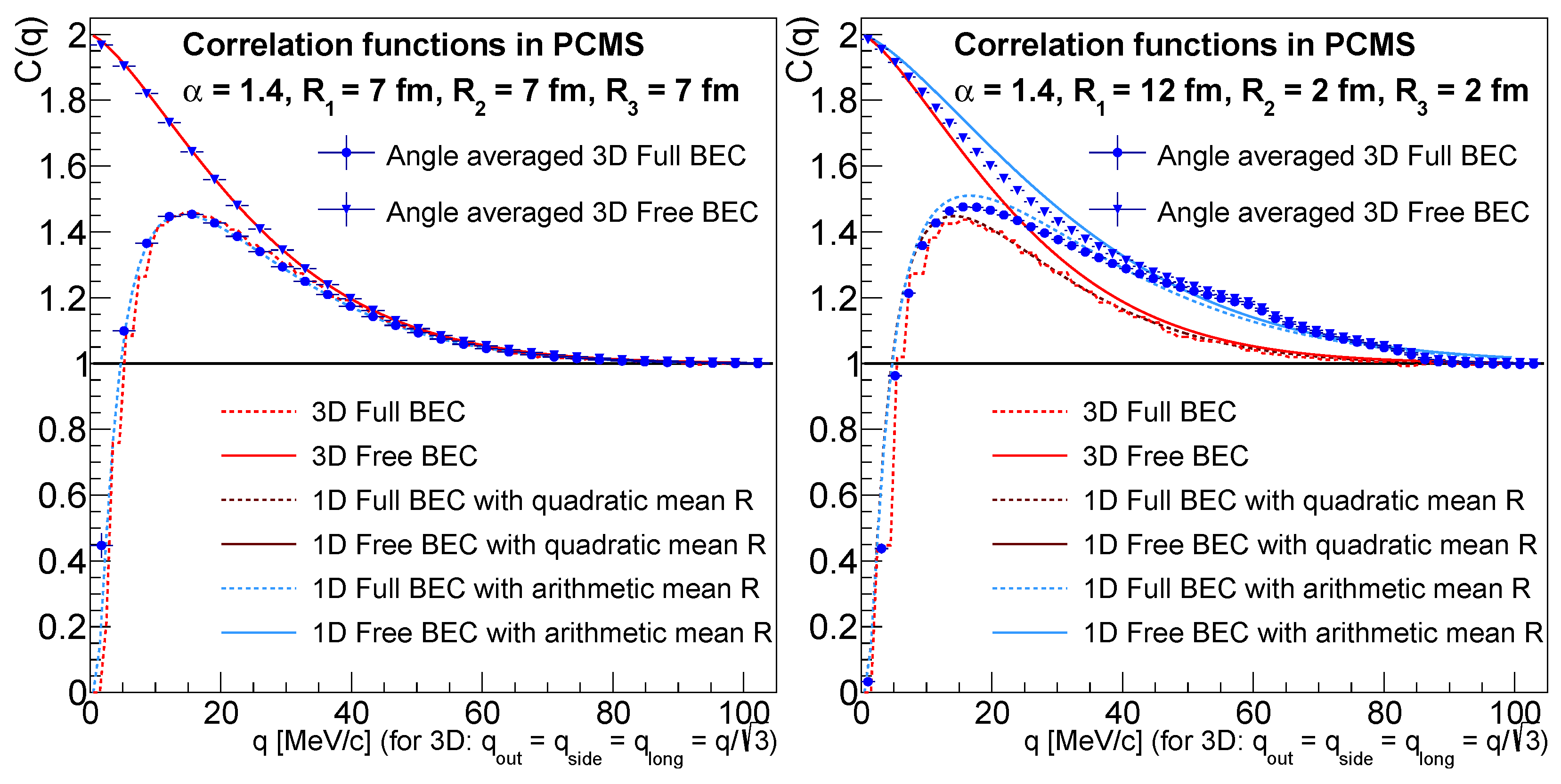
Three-dimensional calculations are rather time-consuming, and their numerical precision could also be problematic for implementation when investigating experimental data. Instead, we aimed to find an approximation that was precise and fast enough to be utilized in actual experimental analyses. Our approach here was that we fixed a set of parameters () and evaluated the integral at points in momentum space. This gave us a fine enough resolution in momentum space for comparison purposes. First, let us compare the two-particle correlation functions in the PCMS. In Figure 1, we can see the Bose–Einstein correlation functions with Coulomb interactions (full BEC) and without any final-state interactions (free BEC) from our 3D calculation and from the 1D calculation with quadratic and arithmetic average scale parameters and the angle averaged values of the 3D calculation. In the spherical case, on the left-hand plot, everything was as we would expect; however, on the right-hand plot, when we had a non-spherical source for the 3D calculation, we can see that there was a large difference between the correlation functions, both in the Coulomb interacting and in the free case.
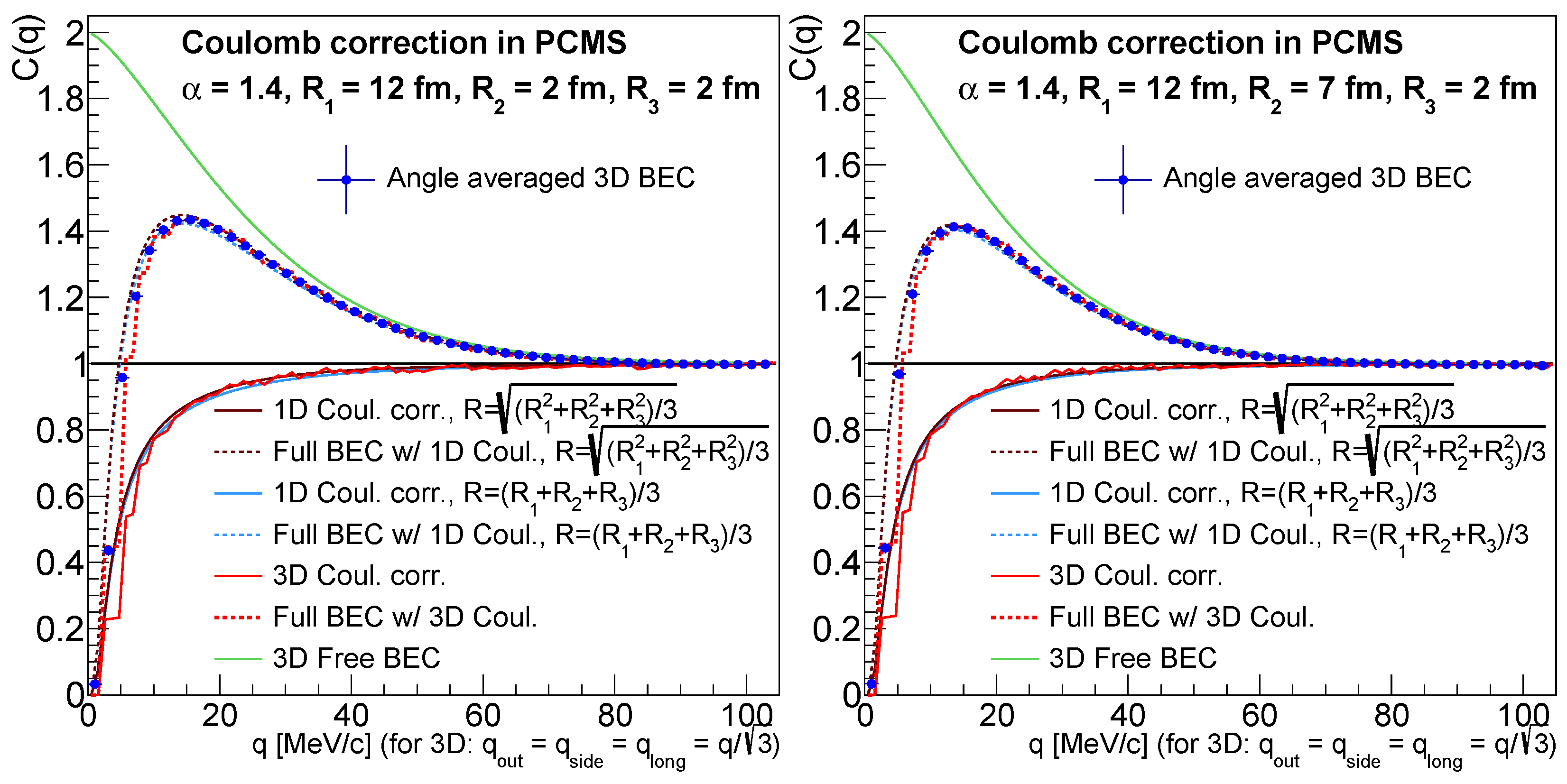
However, we were interested in the question of whether we could use the 1D calculation for the purposes of Coulomb correction only, viz., the ratio of the full and free BEC functions (). One can see the comparison of Coulomb corrections in Figure 2 with two sets of non-spherical parameters. The full BEC functions are here the Coulomb-corrected three-dimensional correlation functions (full BEC ). The one-dimensional Coulomb corrections were evaluated at in the PCMS, i.e., at and at an average R for and . Although the correlation functions were quite different, we can see that the Coulomb corrections were very much the same. Now, we would like to point out the fact that one-dimensional and three-dimensional Coulomb corrections are very similar; therefore, in an experimental analysis, it is sufficient to use a one-dimensional Coulomb correction with the right parameter values. The error caused by the spherical Coulomb correction could be estimated, but it was not in the scope of this paper to give a quantitative limit for this uncertainty.
The application of the Coulomb correction in three-dimensional analyses is quite straightforward. If the measurement is in the LCMS and one has the momenta and the Lévy scale parameters for particles with an average transverse momentum of , which gives , then one proceeds as follows. We used the assumption that the Coulomb correction transformed as a scalar. We evaluated the Coulomb correction (which was calculated in the PCMS) at momenta and scale parameters , , and . Accordingly, we used and an average of , , and when we used a 1D Coulomb correction. For example, we could use the quadratic average:
Therefore, the Coulomb correction that could be applied in a three-dimensional measurement was the following:
where is the result from the integral of Equation (22) in a spherical case with a radius of according to Equation (30) and at momentum , which can be calculated for every point in a three-dimensional measurement in the LCMS.
3.2. Spherical (One-Dimensional) HBT Measurements
Below, we investigate the implications of our calculations for one-dimensional HBT measurements. When we performed a one-dimensional measurement in the LCMS, we assumed that the source was spherical in this frame, i.e., , and we had a single momentum variable . But the Coulomb correction was calculated in the PCMS with . This meant that a spherical source in the LCMS would imply a non-spherical (, ) source in the PCMS and the need for a three-dimensional Coulomb correction. However, we saw above that the non-spherical Coulomb correction could be well approximated with a spherical Coulomb correction if we used the right average R, viz., instead of , we had to use
if we used a quadratic average R. Another problem stemmed from the fact that we could not reconstruct from . An obvious solution would be to measure all momentum variables instead of just the length of the momentum difference, but then the advantage of the 1D measurement over the 3D measurement (the possibility of a measurement with higher statistical significance) would be lost. We could try to overcome this obstacle in some other ways. One solid approximation could be the following: measure an distribution of particle pairs, and then use this to obtain a weighted Coulomb-correction, as shown below.
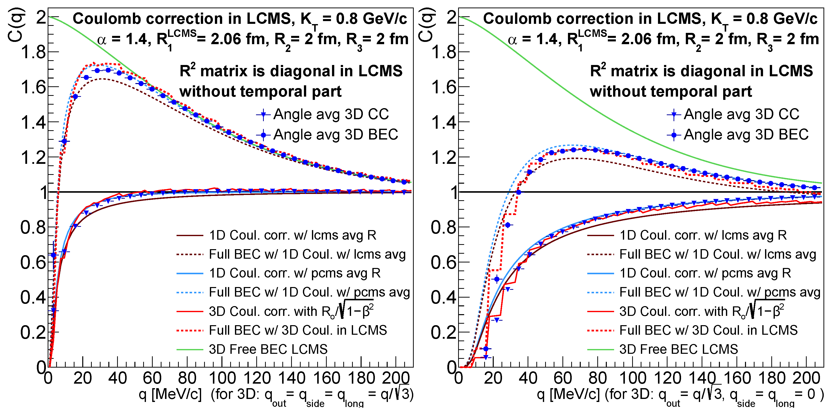
In Figure 3, we see the Coulomb correction and the corrected three-dimensional two-particle correlation functions for GeV/c in the LCMS. The parameters were chosen so that in the LCMS we had an approximately spherically symmetric source ( fm, R fm). We can see that there was a clear difference between the two one-dimensional corrections, with one having an LCMS average R and the other having an average in accordance with Equation (32). In the low-q region, there was some difference between the angle-averaged, one-dimensional, and three-dimensional Coulomb corrections. Also, the numerical precision of the three-dimensional calculation made it challenging to decide between the options. However, we can see that from MeV/c, the angle-averaged and the three-dimensional Coulomb correction were in good agreement with the one-dimensional Coulomb correction with the average R of Equation (32), and there was a consistent difference compared to the other one. The fact that the angle-averaged case was most similar to the one-dimensional case with the transformed average R of Equation (32) indicated that using the latter for one-dimensional measurements was best. On the left-hand side, the three-dimensional correlation function was taken at a diagonal line in the LCMS (), and on the right-hand side along the out axis. We did not rely on a weighted average for the one-dimensional Coulomb correction, as we could calculate .
Let us list the possible approaches to deal with Coulomb interactions in one-dimensional measurements carried out in an LCMS. We only list the options that make use of a one-dimensional calculation for the integral in Equation (22); in these cases, the factor of Ref. [13] can be used. A simpler solution would be to use the Gamow factor, where the source size is neglected. The most sophisticated approach would be to use the angle-averaged Coulomb correction from a three-dimensional calculation, but this would be an overly complex solution. The possibilities for making use of a one-dimensional Coulomb integral calculation are the following, ordered by increasing sophistication:
- Simply use , which means that one formally substitutes and .
- Take into account the fact that but neglect the same for the scale parameters, and use the weighting method of Equation (33); however, implement this not for the Coulomb correction, but for the correlation function instead. Thus, use for the fitting:
- Following the same approach as above, use for the Coulomb correction and use a weighted average, though for the Coulomb correction this time. This approach is more sensible if one considers Figure 1, where we saw that the correlation functions could look rather different even if in Figure 2 the Coulomb corrections looked very much the same. Now, one uses for fitting.
- One improvement to the methods mentioned above would be to consider the transformation of scale parameters; thus, use the average as in Equation (32). The simpler version is the same as no. 3 above, i.e., weighing the correlation function and using for fitting. Here, however, one loses the explicit form of in the LCMS, which is known.
- The most sophisticated option would be to use only for the Coulomb correction and use the weighting of Equation (33). The function used for fitting is now .
- Finally, an approach that is easier to implement than the previous methods making use of a distribution is to make an approximation for the - relationship that is appropriate for the Coulomb correction. One could be motivated by the left-hand plot of Figure 3, as the one-dimensional Coulomb correction with and the angle-averaged three-dimensional calculation were in relatively good agreement. The relationship could be used, as it would hold for the diagonal line . Therefore, the function that could be used for fitting would be .
Additionally, either the distribution of particle pairs from same events (usually denoted with A) or some background distribution that has no quantum-statistical effects (B) could be used for weighting and K [4]. Here, one could argue in favor of the latter; however, it is expected to make a small difference. The soundest approach for one-dimensional analyses is no. 5 in the above list.
4. Conclusions
We investigated Coulomb interactions for HBT measurements in the presence of Lévy sources. Our results can be applied to three-dimensional and one-dimensional measurements alike. The results also hold for Gaussian or Cauchy sources, because these are special cases of the Lévy source ( for Gaussian and for Cauchy). We learned that a one-dimensional Coulomb correction could be reasonably effectively applied for three-dimensional measurements if we used the appropriately defined average of the three directional scale parameters (as in Equation (30) above) and implemented the invariant momentum difference as the momentum variable for the Coulomb correction. For one-dimensional measurements in the LCMS frame, we saw that one should use the average scale parameter as defined in Equation (32) and evaluate the Coulomb correction at as we calculated this in the PCMS frame, which in practice could be estimated with a weighted Coulomb correction according to option no. 5 in the previous section. The above-detailed treatment of Coulomb interactions in heavy-ion collisions could be readily applied to experimental measurements. To our knowledge this indeed has now been achieved in several analyses from SPS through RHIC to LHC, based on the technique outlined in this paper [8,9,20,21,22,23,24].
Author Contributions
Conceptualization, M.C. and B.K.; methodology, M.C. and M.N.; software, B.K., M.N. and D.K.; formal analysis, B.K.; investigation, B.K.; writing—original draft preparation, B.K. and M.C.; writing—review and editing, D.K. and M.N.; visualization, B.K. and D.K.; supervision, M.C.; project administration, M.C.; funding acquisition, M.C. All authors have read and agreed to the published version of the manuscript.
Funding
NKFIH grant No. K-138136.
Conflicts of Interest
The authors declare no conflict of interest.
References
- Csörgö, T. Particle Interferometry from 40 Mev to 40 TeV; NATO Science Series C: Mathematical and Physical Sciences; Springer: Dordrecht, The Netherlands, 2000; Volume 554, Chapter 8; pp. 203–257. [Google Scholar] [CrossRef] [Green Version]
- Bolz, J.; Ornik, U.; Plumer, M.; Schlei, B.; Weiner, R. Resonance decays and partial coherence in Bose-Einstein correlations. Phys. Rev. D 1993, D47, 3860–3870. [Google Scholar] [CrossRef] [PubMed]
- Adamczyk, L.; Adkins, J.K.; Agakishiev, G.; Aggarwal, M.M.; Ahammed, Z.; Alekseev, I.; Alford, J.; Anson, C.D.; Aparin, A.; Arkhipkin, D.; et al. Beam-energy-dependent two-pion interferometry and the freeze-out eccentricity of pions measured in heavy ion collisions at the STAR detector. Phys. Rev. C 2015, C92, 014904. [Google Scholar] [CrossRef] [Green Version]
- Adare, A.; Aidala, C.; Ajitanand, N.N.; Akiba, Y.; Akimoto, R.; Alexander, J.; Alfred, M.; Al-Ta’ani, H.; Angerami, A.; Aoki, K.; et al. Lévy-stable two-pion Bose-Einstein correlations in = 200 GeV Au+Au collisions. Phys. Rev. C 2018, C97, 064911. [Google Scholar] [CrossRef] [Green Version]
- Adler, S.S.; Afanasiev, S.; Aidala, C.; Ajitanand, N.N.; Akiba, Y.; Alexander, J.; Amirikas, R.; Aphecetche, L.; Aronson, S.H.; Averbeck, R.; et al. Evidence for a long-range component in the pion emission source in Au + Au collisions at = 200 GeV. Phys. Rev. Lett. 2007, 98, 132301. [Google Scholar] [CrossRef] [Green Version]
- Afanasiev, S.; Aidala, C.; Ajitanand, N.N.; Akiba, Y.; Alexander, J.; Al-Jamel, A.; Aoki, K.; Aphecetche, L.; Armendariz, R.; Aronson, S.H.; et al. Source breakup dynamics in Au+Au Collisions at = 200 GeV via three-dimensional two-pion source imaging. Phys. Rev. Lett. 2008, 100, 232301. [Google Scholar] [CrossRef] [Green Version]
- Shapoval, V.M.; Sinyukov, Y.M.; Karpenko, I.A. Emission source functions in heavy ion collisions. Phys. Rev. C 2013, 88, 064904. [Google Scholar] [CrossRef] [Green Version]
- Adhikary, H.; Adrich, P.; Allison, K.K.; Amin, N.; Andronov, E.V.; Antićić, T.; Arsene, I.-C.; Bajda, M.; Balkova, Y.; Baszczyk, M.; et al. Measurements of Two-pion HBT Correlations in Be+Be Collisions at 150A GeV/c Beam Momentum, at the NA61/SHINE Experiment at CERN. arXiv 2023, arXiv:2302.04593. [Google Scholar]
- Tumasyan, A.; Wolfgang, A.; Andrejkovic, J.W.; Bergauer, T.; Chatterjee, S.; Damanakis, K.; Dragicevic, M.; Escalante Del Valle, A.; Hussain, P.S.; Manfred, J.; et al. Two-particle Bose-Einstein correlations and their Lévy parameters in PbPb collisions at = 5.02 TeV. arXiv 2023, arXiv:2306.11574. [Google Scholar]
- Kurgyis, B. Three dimensional Lévy HBT results from PHENIX. Acta Phys. Polon. Supp. 2019, 12, 477. [Google Scholar] [CrossRef] [Green Version]
- Sinyukov, Y.; Lednicky, R.; Akkelin, S.V.; Pluta, J.; Erazmus, B. Coulomb corrections for interferometry analysis of expanding hadron systems. Phys. Lett. 1998, B432, 248–257. [Google Scholar] [CrossRef] [Green Version]
- Bowler, M.G. Coulomb corrections to Bose-Einstein correlations have been greatly exaggerated. Phys. Lett. B 1991, B270, 69–74. [Google Scholar] [CrossRef]
- Csanád, M.; Lökös, S.; Nagy, M. Expanded empirical formula for Coulomb final state interaction in the presence of Lévy sources. Phys. Part. Nucl. 2020, 51, 238–242. [Google Scholar] [CrossRef]
- Csörgo, T.; Hegyi, S.; Zajc, W.A. Bose-Einstein correlations for Levy stable source distributions. Eur. Phys. J. 2004, C36, 67–78. [Google Scholar] [CrossRef]
- Pratt, S.; Csörgo, T.; Zimányi, J. Detailed predictions for two pion correlations in ultrarelativistic heavy ion collisions. Phys. Rev. C 1990, C42, 2646–2652. [Google Scholar] [CrossRef]
- Bertsch, G.; Gong, M.; Tohyama, M. Pion Interferometry in Ultrarelativistic Heavy Ion Collisions. Phys. Rev. C 1988, C37, 1896–1900. [Google Scholar] [CrossRef] [Green Version]
- Landau, L.D.; Lifshitz, L.M. Quantum Mechanics Non-Relativistic Theory, 3rd ed.Pergamon Press: Oxford, UK, 1977; Volume 3. [Google Scholar] [CrossRef]
- Metropolis, N.; Rosenbluth, A.W.; Rosenbluth, M.N.; Teller, A.H.; Teller, E. Equation of state calculations by fast computing machines. J. Chem. Phys. 1953, 21, 1087–1092. [Google Scholar] [CrossRef] [Green Version]
- Hastings, W.K. Monte Carlo Sampling Methods Using Markov Chains and Their Applications. Biometrika 1970, 57, 97–109. [Google Scholar] [CrossRef]
- Lökös, S. Probing the QCD Phase Diagram with HBT Femtoscopy. Acta Phys. Polon. Supp. 2022, 15, 30. [Google Scholar] [CrossRef]
- Mukherjee, A. Kaon femtoscopy with Lévy-stable sources from = 200 GeV Au + Au collisions at RHIC. Universe 2023, 9, 300. [Google Scholar] [CrossRef]
- Porfy, B. Femtoscopic correlation measurement with symmetric Lévy-type source at NA61/SHINE. Universe 2023, 9, 298. [Google Scholar] [CrossRef]
- Kórodi, B. Centrality dependent Lévy HBT analysis in = 5.02 TeV PbPb collisions at CMS. Universe 2023, 9, 318. [Google Scholar] [CrossRef]
- Kovács, L. Charged kaon femtoscopy with Lévy sources in = 200 GeV Au+Au collisions at PHENIX. Submitted to Universe. 2023. [Google Scholar]
Figure 1.
On the left-hand side, the two-particle correlation functions are shown in a spherical case for the three-dimensional calculation in comparison with one-dimensional calculations in the presence of Coulomb interactions in final-state interactions. On the right-hand side, a non-spherical three-dimensional calculation is shown alongside one-dimensional calculations with quadratic and arithmetic mean scale parameters.

Figure 2.
The Coulomb corrections and the Coulomb-corrected three-dimensional two-particle correlation function is shown in two non-spherical cases.
Figure 2.
The Coulomb corrections and the Coulomb-corrected three-dimensional two-particle correlation function is shown in two non-spherical cases.

Figure 3.
The Coulomb corrections and the Coulomb-corrected three-dimensional two-particle correlation function are shown in the LCMS when the source was spherical in the LCMS but not for the calculation. On the left-hand side, we took the three-dimensional Coulomb correction along a diagonal line, and on the right-hand side along the axis.

Disclaimer/Publisher’s Note: The statements, opinions and data contained in all publications are solely those of the individual author(s) and contributor(s) and not of MDPI and/or the editor(s). MDPI and/or the editor(s) disclaim responsibility for any injury to people or property resulting from any ideas, methods, instructions or products referred to in the content. |
© 2023 by the authors. Licensee MDPI, Basel, Switzerland. This article is an open access article distributed under the terms and conditions of the Creative Commons Attribution (CC BY) license (https://creativecommons.org/licenses/by/4.0/).
Share and Cite
MDPI and ACS Style
Kurgyis, B.; Kincses, D.; Nagy, M.; Csanád, M. Coulomb Corrections for Bose–Einstein Correlations from One- and Three-Dimensional Lévy-Type Source Functions. Universe 2023, 9, 328. https://doi.org/10.3390/universe9070328
AMA Style
Kurgyis B, Kincses D, Nagy M, Csanád M. Coulomb Corrections for Bose–Einstein Correlations from One- and Three-Dimensional Lévy-Type Source Functions. Universe. 2023; 9(7):328. https://doi.org/10.3390/universe9070328
Chicago/Turabian StyleKurgyis, Bálint, Dániel Kincses, Márton Nagy, and Máté Csanád. 2023. "Coulomb Corrections for Bose–Einstein Correlations from One- and Three-Dimensional Lévy-Type Source Functions" Universe 9, no. 7: 328. https://doi.org/10.3390/universe9070328
Note that from the first issue of 2016, this journal uses article numbers instead of page numbers. See further details here.