
Designing Parameters to Reshape the Inverter Output Impedance Based on the D-Split Method under Weak Grid Conditions


School of Electrical and Control Engineering, Shaanxi University of Science and Technology, Xi’an 710021, China
*
Authors to whom correspondence should be addressed.
Electronics 2023, 12(24), 5000; https://doi.org/10.3390/electronics12245000
Submission received: 8 November 2023
/
Revised: 11 December 2023
/
Accepted: 12 December 2023
/
Published: 14 December 2023
(This article belongs to the Section Industrial Electronics)
Abstract
:Novel energy generation technologies, such as high-permeability wind power and photovoltaic systems, exhibit inherent intermittency, randomness, and volatility. During periods of energy production from these sources, the impedance of the electrical grid frequently experiences significant fluctuations. Consequently, the grid manifests characteristics akin to a weak grid, highlighting the challenges associated with integrating renewable energy sources with variable output profiles. These fluctuations lead to a shift in resonance spikes of the LCL-type filter towards the lower frequency band, consequently impacting the stability of inverter grid connections. To mitigate this issue, the present study introduces a novel approach integrating the D-split method and a proportional–differential feedforward strategy. This combination aims to reshape the inverter’s output impedance, ensuring its consistent stability even amidst significant fluctuations in grid impedance. In this research, the optimal controller parameters for systems operating under robust grid conditions are initially determined. This selection process involves the application of the D-split method, supported by graphical visualization. Additionally, the amplitude and phase angle margin tester is employed while considering the system bandwidth as a limiting constraint. Moreover, accounting for the influence of grid impedance, the D-split method is reapplied to ascertain the most suitable values for the proportional–differential feedforward parameters. This adjustment aims to enhance the adaptability of the grid-connected inverter specifically in scenarios characterized by a weak grid. The hardware-in-the-loop (HIL) simulation results demonstrate that despite the presence of harmonics within the grid and a short circuit impedance ratio (SCR) of 3, the inverter maintains grid stability and effectively suppresses harmonics. Moreover, the total harmonic distortion factor (THD) of the grid-connected current remains below 5%.
1. Introduction
With the widespread adoption of renewable energy generation, inverters serve a pivotal function as converters facilitating the integration of new energy sources into the utility grid [1]. Owing to the distributed nature of renewable energy generation, extended transmission lines, the leakage inductance of distribution transformers, and the escalating influx of new energy sources, the grid connection point for inverters presents a notably high equivalent impedance [2]. Consequently, the power grid exhibits characteristics of a weak grid, posing challenges for seamless integration and control of the inverter within the grid.
To address the challenges posed by the weak grid in relation to grid-connected inverter control, researchers have employed various methodologies to analyze and enhance the stability, resilience, and resistance to external interference within the grid-connected system. Generally, the methods refined by scholars can be categorized into two main groups. The first involves optimizing inverter control parameters to bolster adaptability to weak grid conditions. The second focuses on enhancing inverter performance under weak grid scenarios by incorporating feedforward methods within the grid-connected control structure. This includes strategies such as grid voltage feedforward, capacitor current feedforward, and other related methodologies.
In accordance with references in study [3], it is noted that in conditions characterized by a weak grid, a coupling phenomenon exists between the phase-locked loop and current loop control. This coupling exerts an influence on the stability of inverter grid-connected operations. To mitigate this influence, study [3] introduces a strategy devoid of a phase-locked loop, effectively sidestepping its impact on grid-connected current. In accordance with the insights presented in study [4], it is elucidated that the principal instigator of current resonance in inverters, particularly under conditions of substantial grid impedances, is attributed to high bandwidth phase-locked loops. Furthermore, the article asserts that a reduction in the bandwidth of phase-locked loops serves as an effective means to diminish their impact on grid-connected currents. Studies [5,6] indicate that the existence of grid impedance introduces a positive feedback loop within the inverter control system, consequently impacting the stability of the inverter’s connection to the grid. Research outlined in study [7] demonstrates that integrating direct grid voltage feedforward in weak grids can mitigate the impact of grid background harmonics. However, this integration leads to a reduction in the phase margin of the current control. Study [8] sustains a consistent phase angle margin within the grid-connected system through adaptive controller parameter adjustments grounded in the principles established in [7]. Study [9] fortifies system stability through the integration of a dual second-order filter model in series after the controller. The strategy involves leveraging the inherent 180-degree phase lag property of the dual second-order filter. This ensures that the system’s open-loop transfer function traverses the −180-degree phase in advance of the resonant frequency associated with the LCL filter, thereby contributing to an augmentation in system stability. Proposed in study [10], the integration of a proportional–integral method in series with the capacitor current feedback loop is proposed to enhance the inverter’s adaptability to weak grids and background harmonics. However, this method overlooks the control delay inherent in the inverter. Described in study [11], an adaptive approach is employed to control the quantity of resonant controllers linked in series with the grid voltage feedforward loop, aiming to achieve grid harmonic suppression. However, the method’s implementation is complex. In study [12], an adaptive controller and reconfigurable selective harmonic compensation strategy are introduced. This approach significantly enhances the adaptability and harmonic suppression capability of the inverter in the presence of a weak grid. However, it is noteworthy that this method exacerbates the computational workload associated with the control process. Study [13] enhances the phase angle margin at the impedance crossover frequency by integrating a lead compensator in series within the grid voltage feedforward loop. However, similar to previous methods, it disregards the system delay. Studies [14,15] model the grid-connected inverter and the utility grid as a cascade system, employing impedance analysis methods to evaluate grid-connected stability. The studies propose that the grid voltage feedforward method is analogous to integrating virtual impedances in parallel at both ends of the inverter’s output impedance. Described in study [16], the theory of passive stability concerning inverter output impedance highlights the necessity of a well-designed capacitor current damping coefficient to expand the passive stability region of the system. However, the method’s scope is limited in enhancing the impedance phase angle margin. In the study referenced as study [17], it is highlighted that in the case of higher-order filters, an escalation in grid impedance results in a shift of the resonant spike frequency towards lower frequencies. This shift, in turn, has the potential to induce instability in the system. Study [18] amalgamates capacitor current and grid-side current weighted feedback control to decrease the control order of LCL-filtered inverters. However, this method is developed without accounting for control delay. Study [19] demonstrates the potential to expand the passive stability region of the inverter output impedance by integrating a phase angle lead compensator in series with the capacitor current feedback channel. However, this method introduces challenges in selecting system controller parameters. Studies [20,21] demonstrate that employing the grid voltage feedforward control method creates an impedance interaction between the grid-connected inverter and the utility grid. This interaction may result in harmonic amplification of the grid-connected current during substantial fluctuations in grid impedance, posing a severe risk of system destabilization. Concluding in study [22], the adjustment of controller parameters or structural modifications can improve the inverter’s adaptability to weak grids. Study [23] underscores that within dq asymmetric systems, the coordinate transformation applied in the controllers of three-phase grid-connected converters can engender frequency coupling issues. These challenges intensify with the rise in grid impedance, potentially culminating in severe consequences such as harmonic resonance and system instability. Studies [24,25] introduced the D-split method for parameter selection in both continuous and discrete domains, rendering the process of parameter selection more transparent and intuitive.
In summary, certain existing approaches to enhance grid-connected inverter control in weak grid scenarios overlook system delays, while others that do consider delays often employ methods that render the system control intricate and less intuitive. Moreover, some methods operate within a synchronized coordinate system, neglecting the frequency coupling issues arising from coordinate transformations, rendering them less suitable for practical engineering applications. Further research is imperative to develop an inverter control method characterized by computational efficiency, structural simplicity, intuitiveness, reliability, and ease of application in engineering practices under weak grid conditions.
The objective of this paper is to explore the feedforward parameters of the inverter output impedance reshaping in conjunction with the D-split method, to realize the strong stability and robustness of the inverter to grid impedance variations, and at the same time to show high harmonic suppression capability in case of grid voltage misalignment. In this study, a quasi-proportional-resonant (QPR) controller is selected to prevent loop coupling within the synchronous reference frame. The impedance criterion is employed to amalgamate the grid voltage feedforward method with the D-split method, aiming to attain a stable parameter domain through the visualization form of the D-split method. The system bandwidth and the suppression of background harmonics serve as individual constraints, with two successive selections of the most suitable parameters within the stability domain. In conclusion, the final outcome involves reshaping the inverter’s output impedance to ensure that both the inverter’s output impedance and the grid impedance crossover frequency consistently remain within the passive stabilization region. This adjustment significantly enhances the suppression of grid-connected currents against background harmonics and bolsters the adaptability and dynamic response of the grid-connected inverter, especially in scenarios involving a weak grid.
The rest of the paper is organized as follows. Section 2 develops a mathematical model of the grid-connected inverter with LCL filter. Section 3 describes the principle and conditions of use of the D-split method, and the steps for designing the key parameters to enhance the adaptability of the inverter to a weak grid using the D-split method. Section 4 describes the controller parameterization method for determining the maximum control bandwidth using the D-split method under a strong grid. Section 5 describes the inverter output impedance modeling under weak grid and the use of D-split method to reshape the inverter output impedance. Section 6 verifies the validity of the proposed theory through semi-physical simulation with RTLAB setup in the HIL. Section 7 summarizes the whole paper and suggests the future research direction of this paper.
2. Modeling of the Inverter
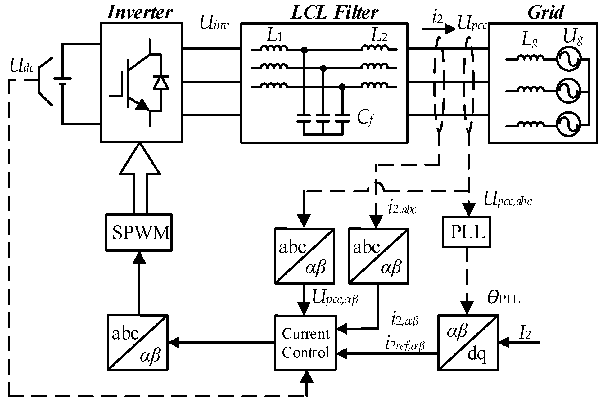
Figure 1 illustrates the circuit topology and control strategy employed in a three-phase LCL-filtered grid-connected inverter. Here, Udc represents the direct current bus; L1 denotes the inverter-side inductor; L2 signifies the grid-side inductor; and Cf indicates the filter capacitor. The grid impedance (Lg) along with the AC voltage source (Ug) collectively establish a weak grid. Considering that the resistive element within the grid impedance bolsters the stability of the inverter during grid-connected operations, this analysis focuses on the worst-case scenario, assuming neglect of the grid line resistance [26].
The grid-connected control strategy process is depicted in Figure 1. The voltage at the grid common coupling point (Upcc,abc) serves as an input to the phase-locked loop (PLL) in order to generate the grid operating phase angle (θPLL). The commanded magnitude of the grid-connected current (I2) is converted inversely into Park coordinates, transforming it into the αβ-frame to generate the current-reference signals (i2ref,αβ). The grid-connected current (i2,abc) and the voltage at the common coupling point (Upcc,abc) undergo a Clark transformation to generate the signals i2,αβ and Upcc,αβ. These signals, along with the current feed signals (i2ref,αβ), are collectively directed into the current controller for processing. Subsequently, the switching signals for the power transistors are derived via the current loop, coordinate transformation, and sinusoidal pulse width modulation (SPWM). This series of processes ultimately achieves the grid connection of the inverter unit power.
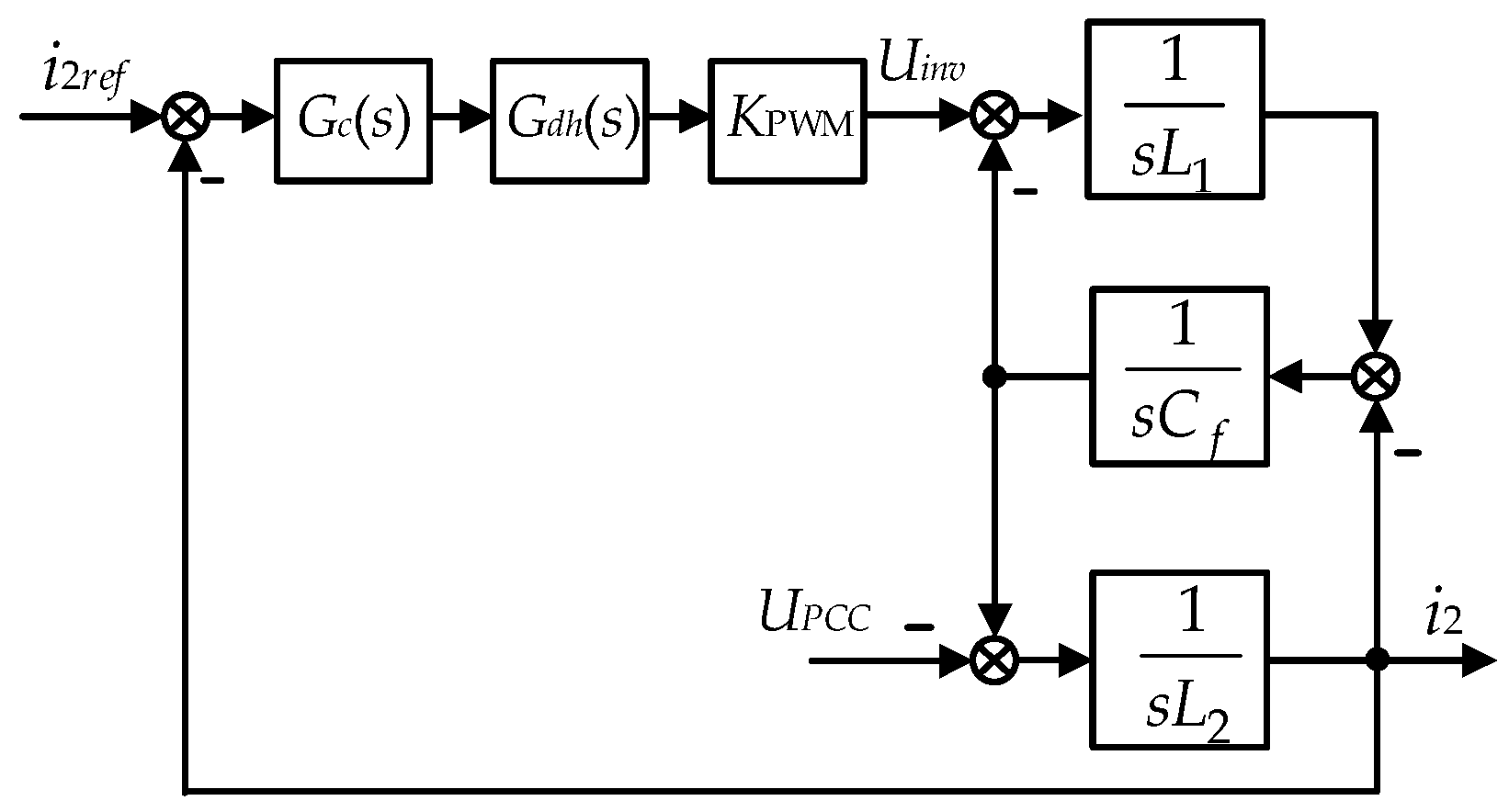
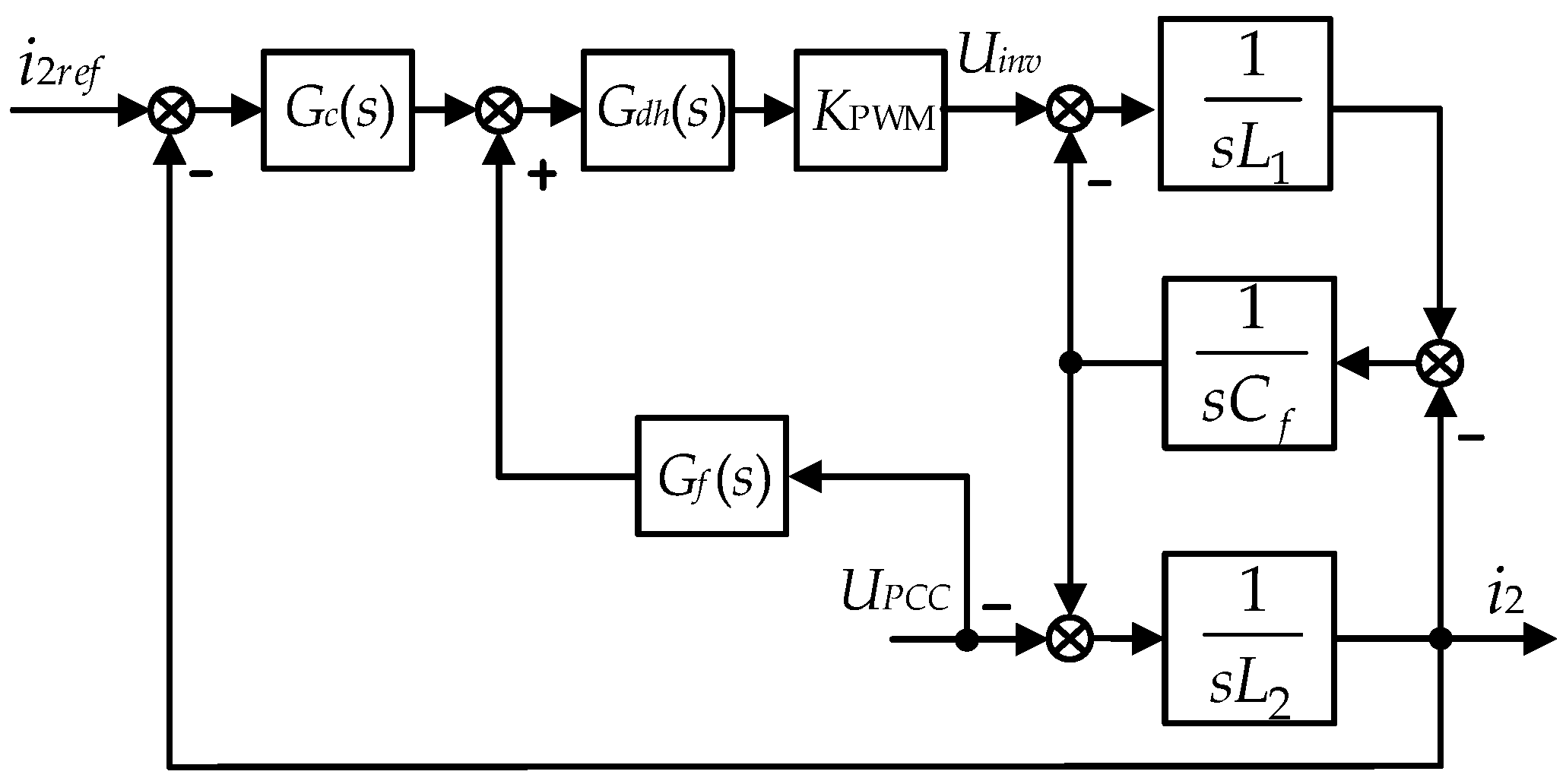
The control configuration of the three-phase grid-connected inverter in the αβ-frame is depicted in Figure 2. Due to the symmetry of the α and β axes, the subscripts of the variables are omitted in this context.
The transfer function from the grid-side current (i2) to the inverter output voltage (Uinv) is expressed as follows:
In contrast to the PI controller, the QPR controller exhibits significantly higher gain at the resonance frequency, facilitating precise tracking of the current-given signals (i2ref) by the grid-side current (i2) without any static error. This characteristic is mathematically expressed as:
where Kp represents the proportionality coefficient, Kr denotes the resonance coefficient, ωc stands for the controller bandwidth, and ωo represents the resonance angular frequency of the controller. Here, ωo corresponds to the electrical angular frequency of the grid, set at 314 rad/s. To guarantee the controller’s adequate gain in case of a grid frequency fluctuation within ±0.5 Hz, ωc = π rad/s is selected in this context [27].
Given the presence of computational delays and modulation delays in practical scenarios involving digital processors, these can be approximated as one-step delays and zero-order hold, respectively. The frequency response of the sampling switch within the Nyquist frequency range (half of the sampling frequency) is 1/Ts. Therefore, a 1/Ts needs to be connected in series on the feedback path of i2 within the control block diagram illustrated in Figure 2. Consequently, the system delay model can be expressed as follows [28]:
KPWM represents the bridge arm gain coefficient of the grid-connected inverter [29], denoted as:
where Udc denotes the DC side voltage of the inverter, while Utri represents the carrier amplitude. To safeguard the inverter operation from disruptions originating on the DC source side and to mitigate changes in the system’s open-loop gain, this paper introduces a decoupling link denoted as 1/KPWM in the control loop. This addition is implemented through the dynamic detection of the DC bus voltage. Consequently, the KPWM value within the inverter control loop is maintained at a constant value of 1.
By deriving Equations (1)–(4), the open-loop transfer function of the grid-connected inverter can be expressed as follows:
The closed-loop transfer function of the system can be derived from Equation (5) as:
Utilizing Equations (5) and (6), the characteristic equation of the grid-connected inverter can be obtained as follows:
3. Theoretical and Parametric Design Procedures for the D-Split Method
3.1. Principles of the D-Split Method
The D-split method is derived from the parameter space method and provides convenience in designing systems with multi-parameter constraints. If the closed-loop characteristic equation contains control delay in the following form:
where ci(k) and di(k) represent continuous functions with respect to n system parameters k = (k1,k2,kn). The characteristic polynomial D(s;k) exhibits a finite number of right half-plane zeros if l > r, or if l = r and |di(k)| < 1. Therefore, the D-split method can be employed to define the stability domain of the controller parameters.
Based on the quantity of zeros in the characteristic polynomial situated within the right half-plane, the domain for the parameter under investigation can be subdivided into multiple sections expressed as D(g,f), where g = 0,1,2, …, f. Here, g signifies the count of positive real roots present in the characteristic polynomial of the closed-loop system within that block of the controller parameter domain, along with f-g representing the negative real roots. Therefore, one can correlate the domain of stabilizing parameters for the resolved system to the area D(0,f) within the D-split method.
For Equation (8), by ordering the s terms in ascending powers, one can express:
Then the boundary of the D-split method is defined as follows:
where D0 and D1 are referred to as singularly stable boundary lines, while D2 is denoted as the non-singularly stable boundary line. The parameter points within each region partitioned by the aforementioned boundaries share an equivalent count of right half-plane zeros.
3.2. Designing Stabilization Domain Parameters Based on the D-Split Method Involves the following Steps
The design flowchart is illustrated below:
1. By disregarding the grid impedance, the characteristic equation for the grid current output, i2(s)/i2ref(s), is derived, which, when combined with Equation (10), enables the determination of the stability domain for the system’s controller parameters.
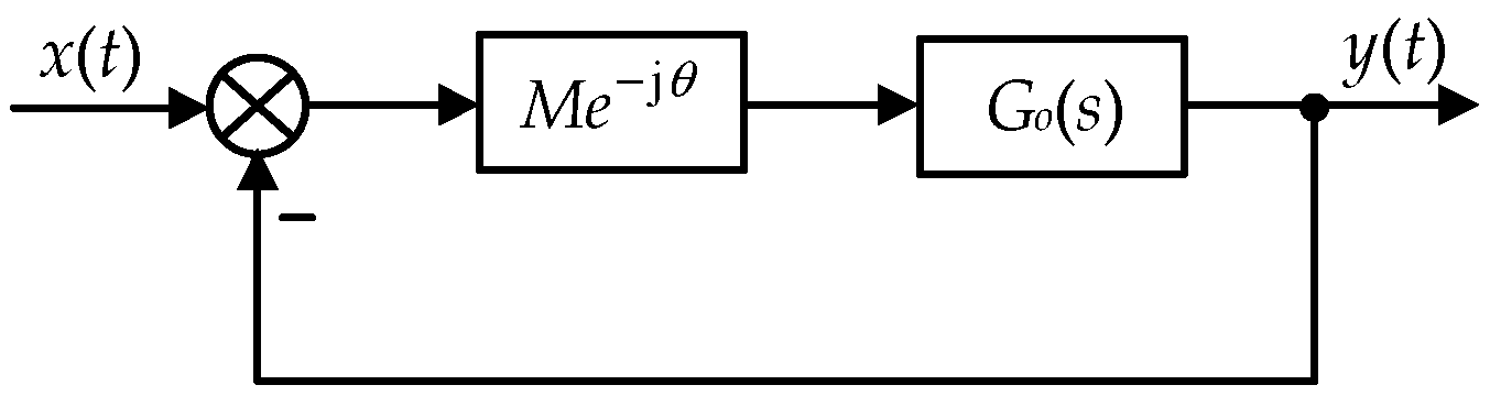
2. Additionally, in tandem with the phase angle-gain tester depicted in Figure 3, specific values are assigned for the desired magnitude margin, M, and the desired phase angle margin, θ, to extract a fresh characteristic equation for the system. The equation is then integrated with Equation (10) to delineate the stability domain of the system’s controller parameters, which encapsulates the desired magnitude-phase angle margin.
3. In the parameter domain obtained in step 2, the system bandwidth information is utilized as a constraint to identify the most suitable controller parameters under the condition of no grid impedance.
4. Taking into account the impact of the grid impedance Zg(s), the stability criterion for the impedance is applied to derive the inverter output impedance Zo(s). By iteratively applying step 2, the characteristic equation of Zg(s)/Zo(s) is deduced, leading to the determination of the stability domain for the voltage feedforward parameters. The most suitable voltage feedforward parameters are selected based on increasing the harmonic suppression capability as a constraint.
4. Stability Analysis in the Absence of Grid Impedance
4.1. Stabilized Regions under the D-Split Method
Combining Equations (7), (9), and (10), the critical stabilizing boundary equation of the control system can be derived as indicated in Equation (11).
where:
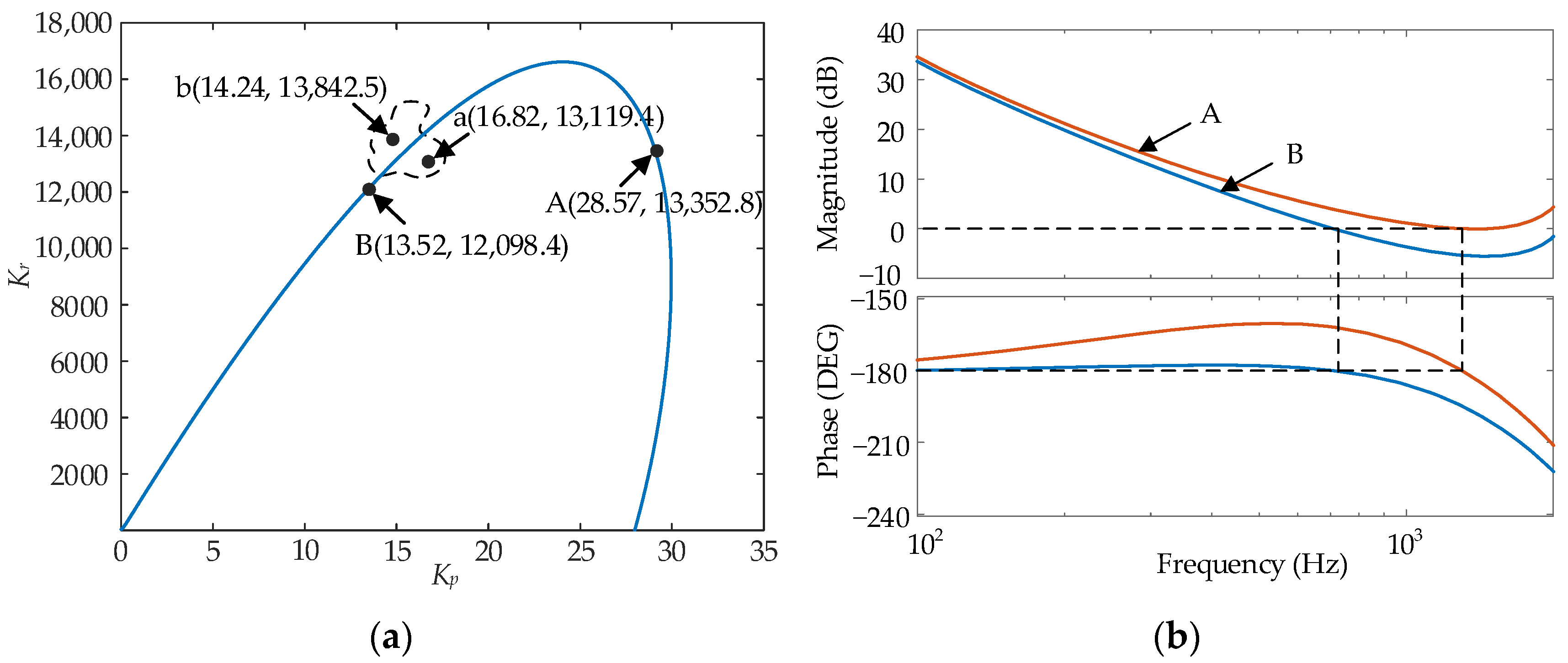
Based on Equation (11), the domain of controller parameters for system stabilization is depicted in Figure 4a.
Two parameter points, A and B, were chosen from the critical boundary curve in Figure 4a and incorporated into Equation (5) to produce the Bode plot illustrated in Figure 4b. According to the Nyquist criterion, the count of poles in the right half plane of the open-loop transfer function Equation (5) is represented as p = 0. Meanwhile, the number of positive (N+) and negative (N−) traversals in the Bode diagram is determined as 0 each. Thus, by utilizing Z = P − 2(N ± N−), the number of poles in the right half plane of the closed-loop transfer function Equation (6) is calculated as Z = 0. At this point, the system exhibits stability, with the phase margin of the system being 0 under these two control parameters. The system is critically stable.
4.2. Performance Constraints Related to Amplitude-Phase Angle Mahoweverergin
As depicted in Figure 3, integrating a magnitude-phase angle margin tester in series with the system’s forward path alters the system’s open-loop transfer function, represented by Equation (12). By combining Equations (6), (9) and (10), the stability region of the controller parameters for the system aligns with the targeted amplitude and phase angle margin constraints.
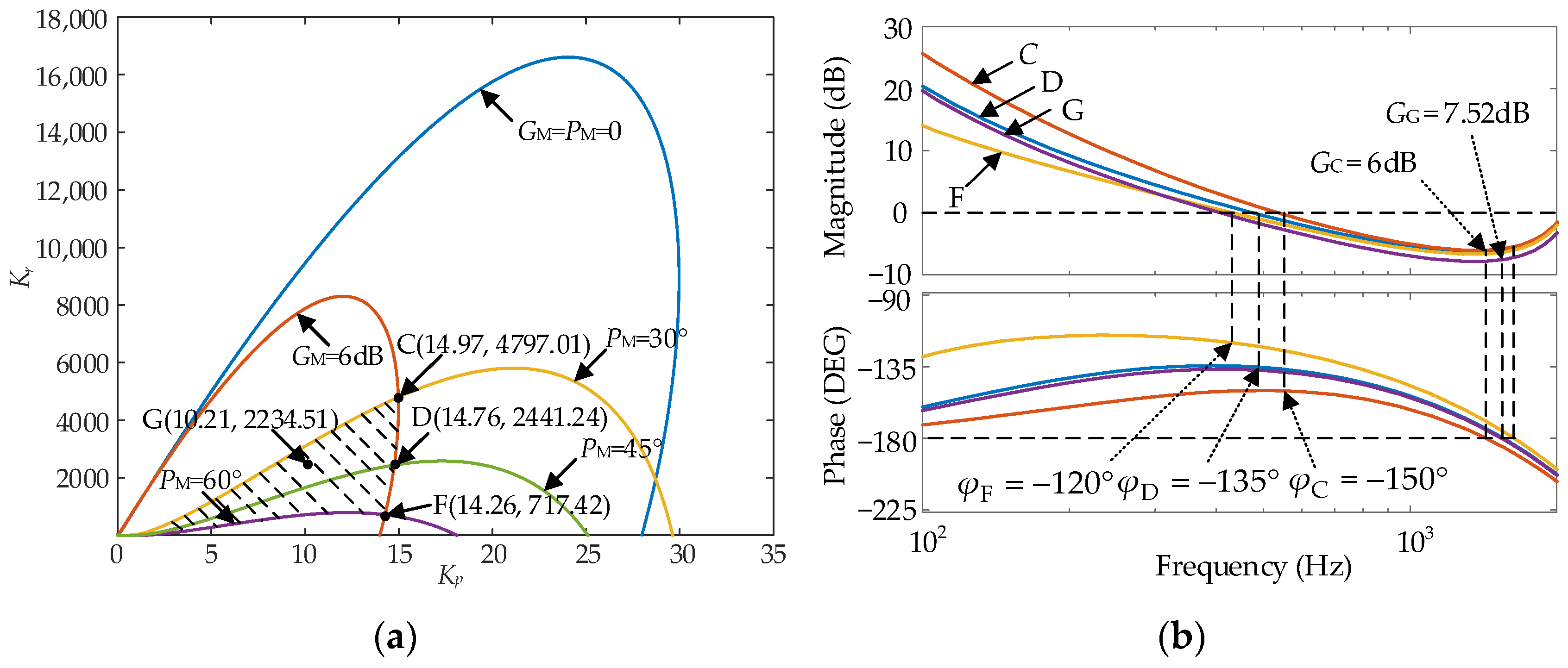
Engineering norms typically mandate a system’s amplitude margin to be above 6 dB, with the phase angle margin ideally ranging between 30° and 60°. By setting M = 2 and θ = 30 in Figure 3, the controller’s parameter stabilization domain is obtained for the multi-objective condition, as depicted in Figure 5a.
To validate the accuracy of the parameter selection, points C and F—representing the two boundary intersection points, along with point G within the shaded region in Figure 5a, are chosen. They are then introduced into Equation (5) to generate the open-loop Bode diagram of the system, presented in Figure 5b. The Bode plots associated with these controller parameters exhibit margins that align with the theoretical analysis, validating the accuracy of the method.
4.3. Analysis and Constraint of System Bandwidth
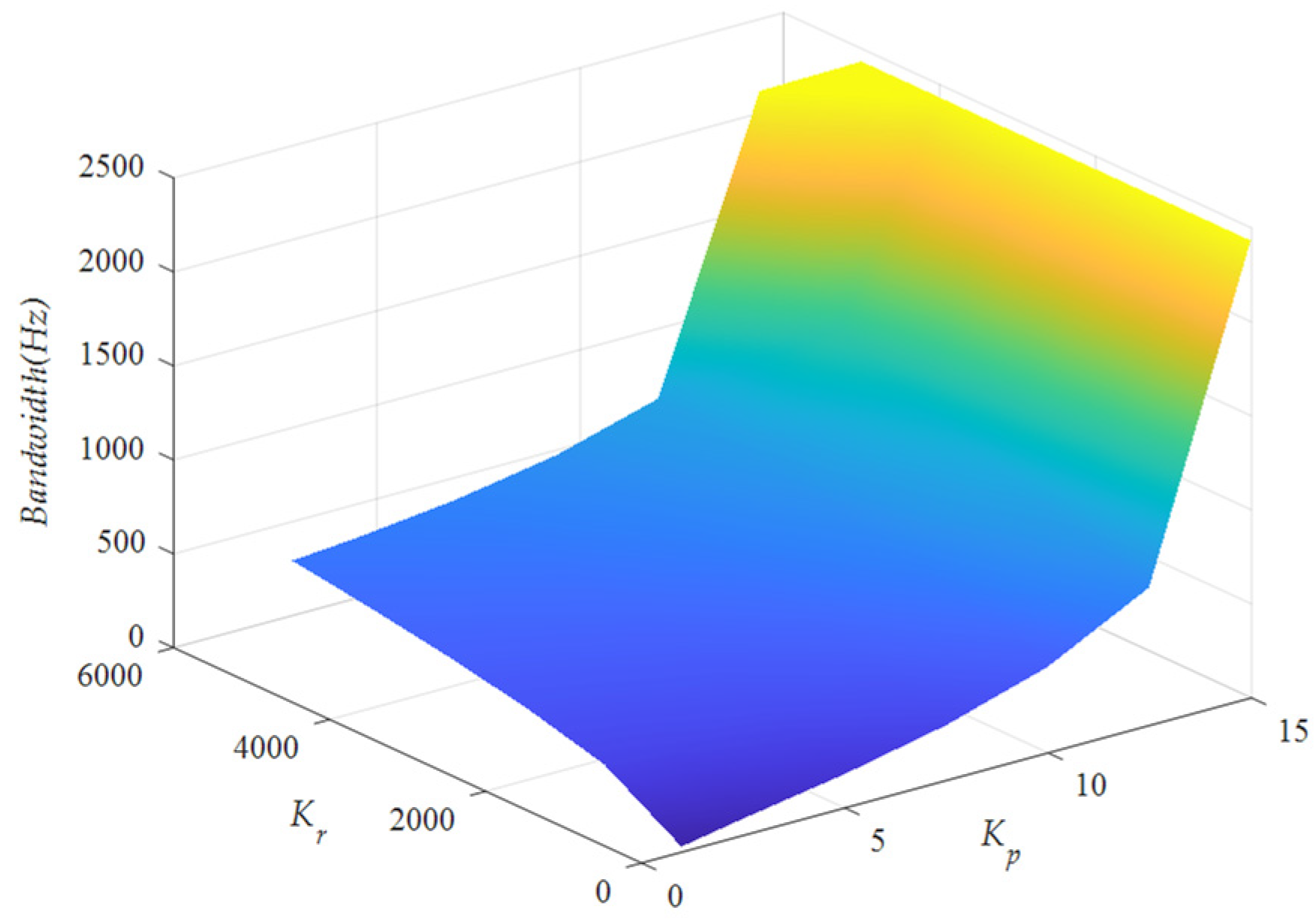
Bandwidth characterizes the dynamic response of a control system. A wider bandwidth indicates a richer information content in the control band and a faster system response. Analyze the bandwidth of the controller parameters found within the shaded region of Figure 5a. Employ Kp as the x-axis, Kr as the y-axis, and the bandwidth frequency as the z-axis. Chart these data points on the three-dimensional graph depicted in Figure 6. It is apparent that, in comparison to Kr, Kp has a more substantial impact on the system’s bandwidth frequency. The Kp values at points D and C in Figure 5a exhibit slight differences, yet point D provides a superior phase margin compared to point C. Consequently, in this scenario, point D is selected as the more suitable controller parameter without grid impedance.
5. Stability Analysis in Weak Grid Conditions
5.1. Analysis of Impedance Stabilization Conditions
The non-negligible grid impedance within a weak grid results in an impedance mismatch between the grid and the grid-connected inverter, consequently causing harmonic distortions in the grid-connected current.
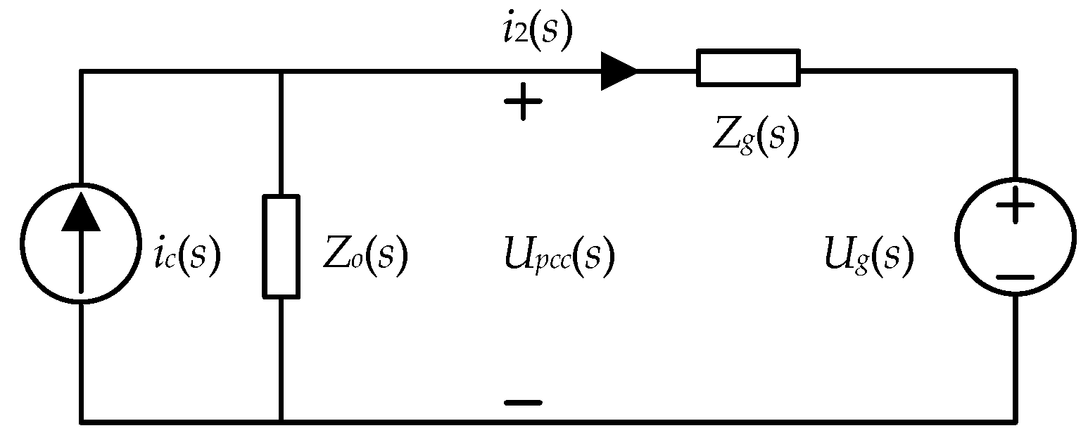
The grid-connected inverter model can be represented as a controlled current source ic(s) running parallel to an output impedance Zo(s). Meanwhile, the weak grid model can be construed as a series connection involving a voltage source, Ug(s), housing a surplus of harmonics, conjoined with the grid impedance, Zg(s). The Norton equivalent circuit model illustrating the inverter’s grid connection under weak grid conditions is depicted in Figure 7 [30].
The expression for the grid-connected current i2(s) at the output of the inverter is as follows:
As per the impedance passive stabilization criterion, the system stabilization necessitates meeting the following two conditions: (i) stability of 1/Zo(s); (ii) fulfillment of the Nyquist stabilization criterion by Zg(s)/Zo(s).
Condition 1 necessitates the inverter’s stability in the absence of grid impedance, which is obtained in Section 4. Condition 2 requires Zg(s)/Zo(s) to exhibit a specific phase margin at an amplitude gain of 0 dB. The phase margin between Zg(s) and Zo(s) at the frequency point ωi, where the amplitude-frequency characteristic intersects, can be expressed as:
Upon considering the minimum phase margin at ωi when the grid impedance Zg(s) is inductive, Equation (14) can be expressed equivalently as:
According to Equation (15), the phase margin of the inverter control system remains positive as long as the phase of the inverter output impedance Zo(s) and the grid impedance Zg(s) at the magnitude intersection are greater than −90°. Furthermore, from Equation (13), it becomes apparent that to mitigate the harmonic effects originating from the voltage at the PCC, the impact of that voltage harmonic on the grid-connected current diminishes when the amplitude gain of the inverter output impedance Zo(s) is higher at a specific voltage harmonic frequency. Hence, to enhance the robustness of the grid-connected inverter system, the following improvements need to be implemented.
1. Increase the amplitude of the inverter output impedance Zo(s) to attenuate grid harmonic disturbances.
2. Enhanced the phase margin at the cutoff frequency of the inverter output impedance Zg(s)/Zo(s).
Upon integrating a grid-connected inverter into the grid, the grid stiffness can be assessed through the short circuit capacity ratio (SCR) [31]. Conventionally, a grid is classified as weak when SCR ≤ 5, and as very weak when 2 < SCR < 3. This classification serves as a basis for introducing the grid impedance value, expressed as follows:
where Vn signifies the rated voltage of the grid, and Sn denotes the rated power of the inverter in the grid-connected system.
5.2. Strategy of Grid Voltage Feedforward
To mitigate the current oscillation resulting from the discrepancy between the inverter output and the grid impedance, a PCC voltage feedforward strategy is commonly employed to improve the phase angle margin of Zg(s)/Zo(s) [32]. In this paper, the series connection of a proportional–differential model to the grid voltage feedforward loop is represented by the functional expression [33]:
where nCfs represents the differential model, n stands for the differential adjustment factor, Cf denotes the filter capacitor, and m indicates the proportional adjustment factor.
The diagram representation of the proportional–differential feedforward control integrated with grid voltage is depicted in Figure 8.
The expression for the grid-connected current i2(s) of the grid-connected inverter is:
The inverter output impedance Zo(s) can be obtained from Equation (18) as follows:
The closed-loop characteristic equation for the open-loop transfer function Zg(s)/Zo(s) can be further deduced from Equation (19) as follows:
Examining equation (20), it becomes evident that the equation involves four variables—m, n, Kp, and Kr—establishing a coupling relationship between m and n (representing voltage feedforward parameters) and Kp and Kr (representing controller parameters). To advance our methodology, it is imperative to eliminate this coupling relationship, facilitating the determination of feedforward parameters through the D-split method. A comparison between Equations (8) and (20) reveals that the D-split method allows for the determination of feedforward ratio (m) and differential coefficient (n) values when the values of Kp and Kr are held constant. This observation aligns with the methodologies employed in Section 2, Section 3 and Section 4 of this paper.
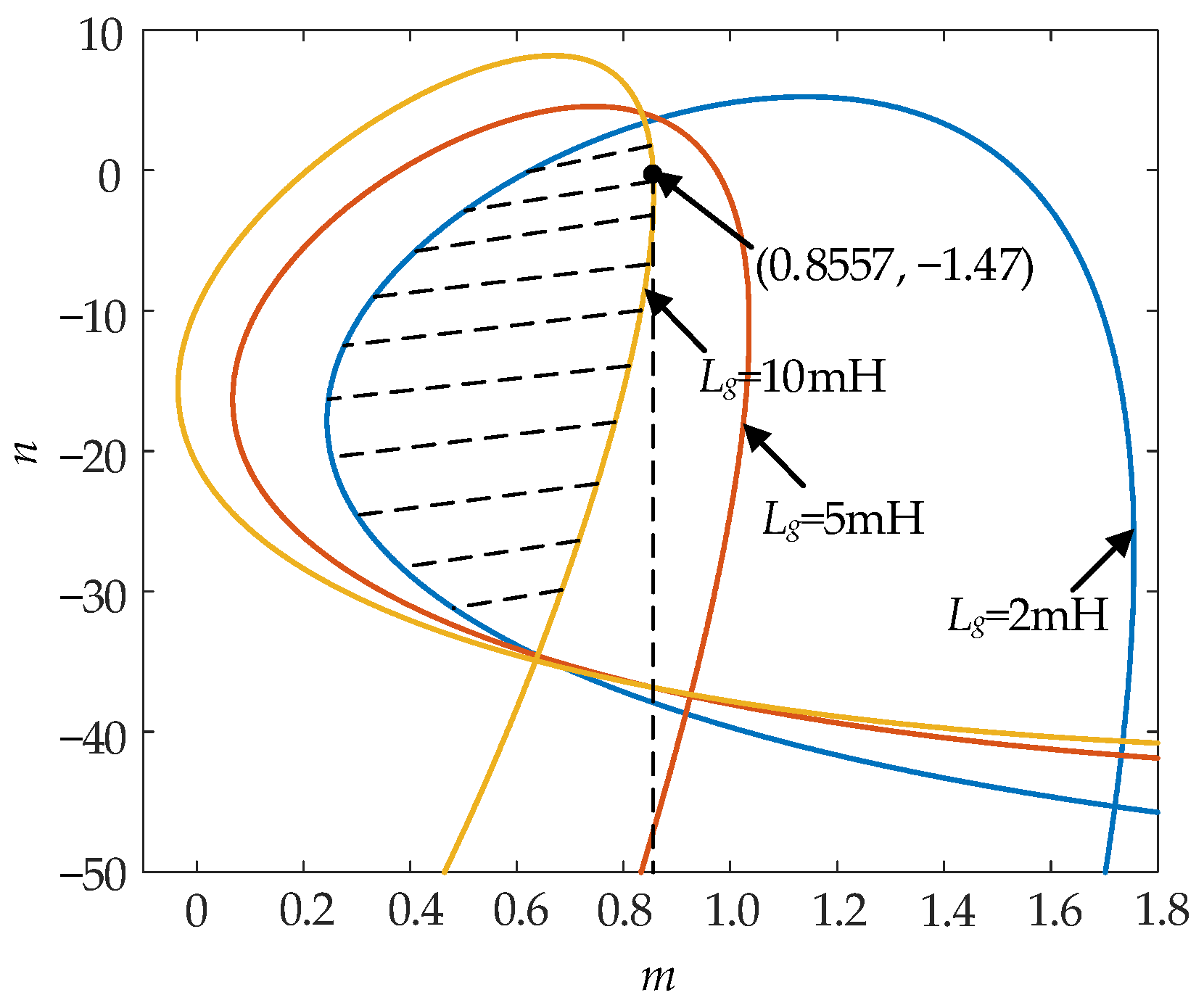
Introducing the values of Kp and Kr, as determined in Section 4, into Equation (20) and then comparing Equation (20) with Equation (8) indicates that the D-split method can be utilized to delineate the stability domains of m and n under a weak grid once Lg is established. To guarantee the grid-connected inverter’s robust adaptability to the grid impedance under weak grid conditions, a phase angle margin of at least 30° should be maintained at the impedance crossover frequency point ωi. Employing the amplitude-phase angle margin tester illustrated in Figure 3 and fixing M = 1, θ = 30, m and n values can be derived for different Lg. The shaded area in Figure 9 represents the shared stabilization domain for the parameters m and n across various Lg values.
5.3. Determination of Optimal Parameters for Grid Voltage Feedforward
Per the Equation (19), it is evident that the grid voltage feedforward occurs solely in the denominator of the inverter output impedance. The range of values for m is determined by initially setting n = 0 in Gf(s) and focusing solely on the effect of m on the amplitude-frequency characteristic |Hm| and phase-frequency characteristic φm of the output impedance denominator. The corresponding value of n for a given m is then derived from the stabilized region of the parameter shown in Figure 9. The expressions for the amplitude-frequency characteristic and phase-frequency characteristic of the inverter output impedance under the influence of m are depicted in Equations (21) and (22).
Derivation of m in Equation (21) provides an expression for m when the denominator amplitude of the output impedance |Hm| is at its minimum, as shown in Equation (23), and an expression for m when the denominator phase angle is at its maximum, as shown in Equation (24).
To mitigate the impact of low-frequency grid harmonics, it is essential to augment the amplitude of the low-frequency band in the inverter’s output impedance. Given that the impedance crossover frequency ωi of Zg(s) and Zo(s) is typically significantly lower than the switching frequency fs, and neglecting the impact of the filtering capacitor, the low-frequency band can be approximated as ωTs ≈ 0 and ω2L1Cf ≈ 0. Hence, m can be approximated as 1.
Based on the analysis, with an increase in m, the amplitude-frequency characteristic of the inverter output impedance within the low-frequency range becomes larger. Consequently, the frequency point ωi, where Zg(s) and Zo(s) intersect, shifts towards the lower frequencies. Additionally, the phase-frequency characteristic of Zo(s) decreases, leading to a reduction in the phase angle margin of Zg(s)/Zo(s).
When m equals 1, it maximizes the amplitude-frequency characteristic of the inverter output impedance and minimizes the phase-frequency characteristic at that point. When m exceeds 1, the denominator term in Equation (22) changes its sign from positive to negative, inducing a 180° increase in the output impedance denominator phase and a consequent 180° reduction in the phase angle margin. Hence, the value of m spans from 0 to 1.
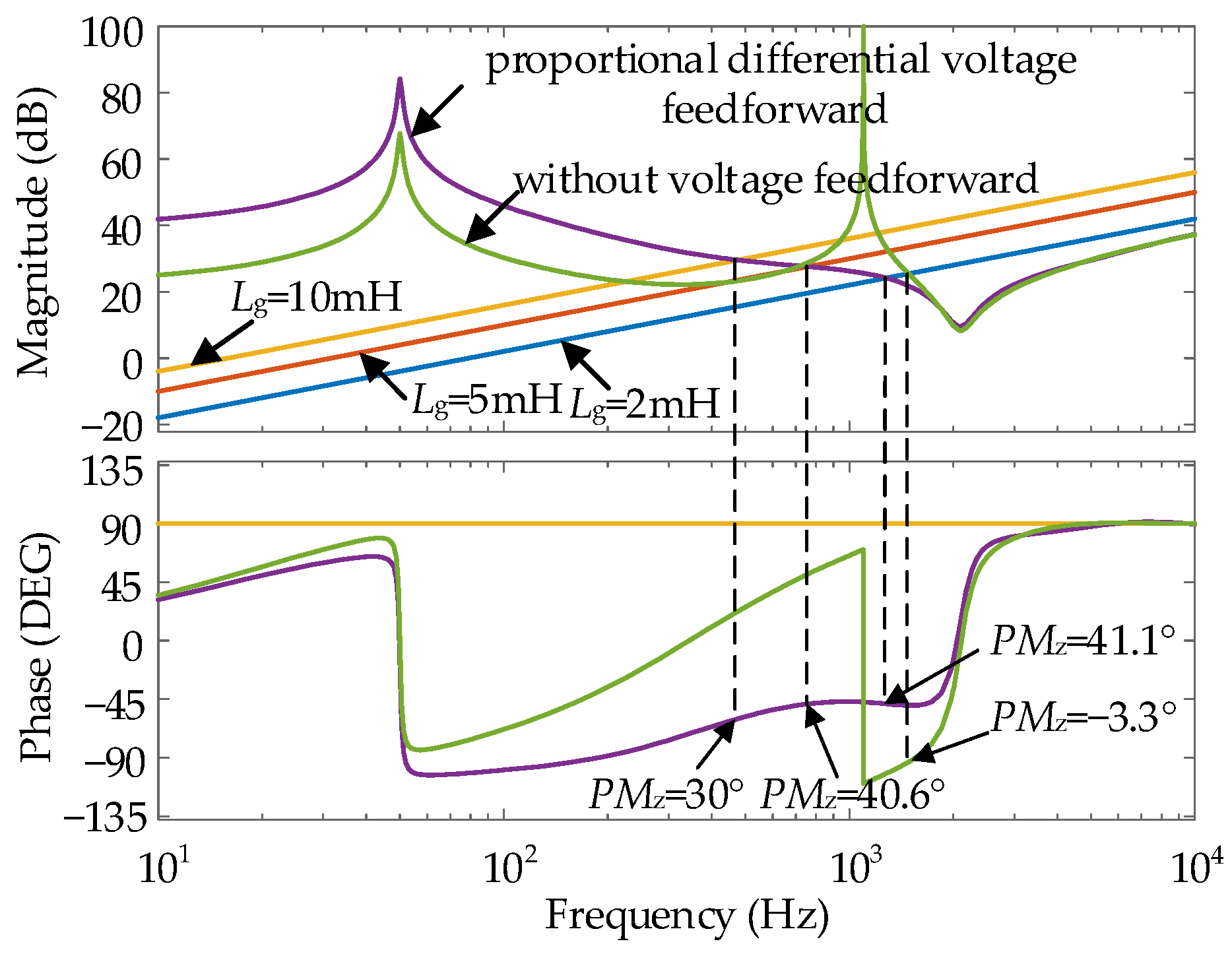
In conclusion, the proportionality coefficient m in the grid voltage feedforward model should be chosen to be close to 1, as it enhances the inverter’s capability to suppress grid harmonics effectively. Given the sensitivity of the differential model to noise, it is advisable to use smaller differential coefficients. Examining the shaded region depicted in Figure 9, the determined values are m = 0.8557 and n = −1.47. In this study, the grid impedance Lg is varied as 2 mH, 5 mH, and 10 mH. The Bode diagrams illustrating the impedance crossings of Zg(s) and Zo(s) under the feedforward parameters are depicted in Figure 10. It is evident that the low-frequency band’s amplitude of the inverter output impedance increases, while the phase angle margin at the frequency point where it intersects with the grid impedance improves, validating the theory’s accuracy.
6. HIL Simulation Results and Analysis
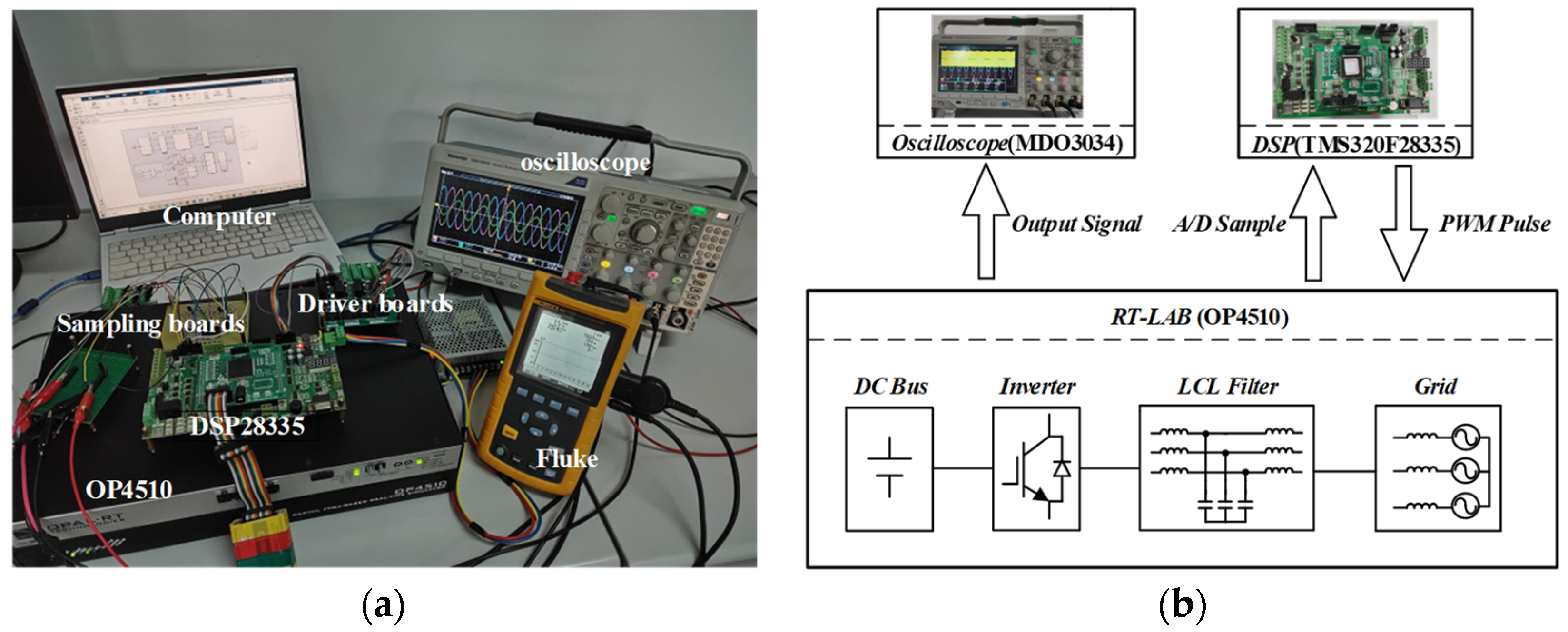
To validate the accuracy and credibility of the aforementioned theory, a three-phase grid-connected inverter HIL setup is constructed using Real Time Laboratory (RT-LAB), illustrated in Figure 11a. Here, the OP4510 serves as the primary circuit, integrated with TI’s TMS320F28355 DSP and an oscilloscope, operating in HIL mode, as depicted in Figure 11b. Given the constrained output voltage of the OP4510 analog output port, the experiment employs a scaling ratio of 25 V/1 V for output voltage measurement and a scaling ratio of 1 A/1 V for current measurement. The parameters of the prototype are shown in Table 1.
6.1. Scenario 1
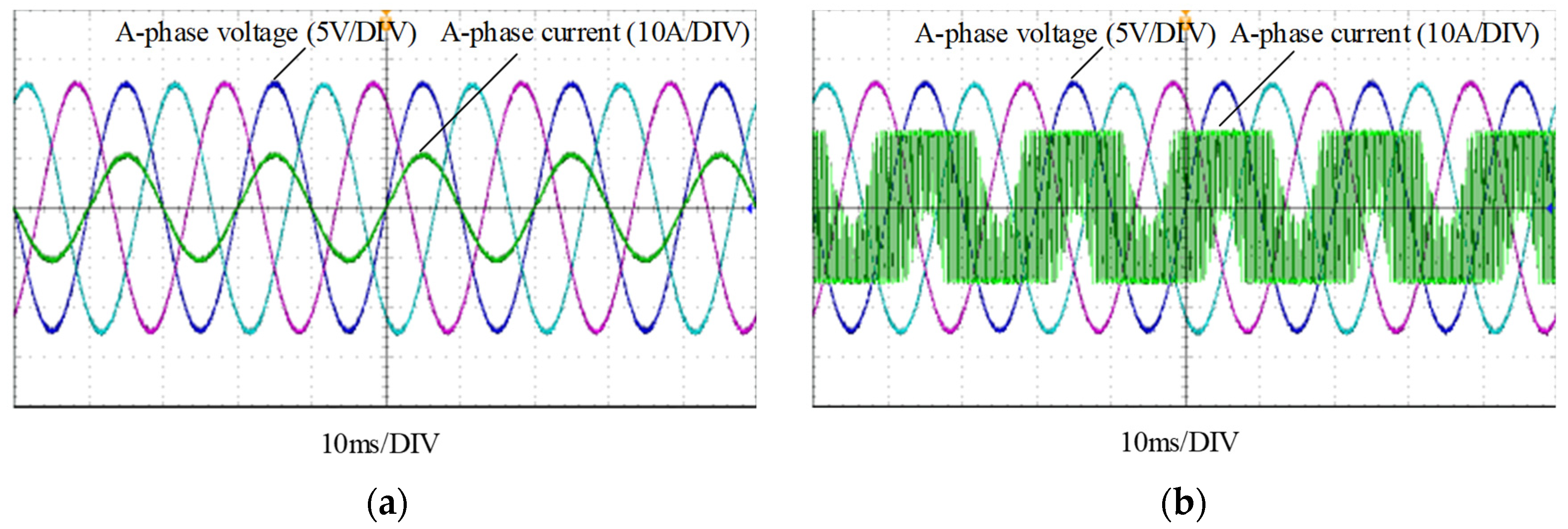
Validation of the correctness and efficacy of the D-split method is conducted. In the absence of grid voltage feedforward and grid impedance, we experimentally analyze point a (16.82, 13,119.4) within the critical region and point b (14.24, 13,842.5) outside the critical region, as depicted in Figure 4. In Figure 12a, it is evident that the grid-connected current maintains stability when operating with the stable controller parameter point ‘a’. Conversely, Figure 12b illustrates the HIL simulation waveforms associated with the unstable controller parameter point ‘b’, displaying a significant presence of harmonics in the grid-connected current, resulting in system instability.
6.2. Scenario 2
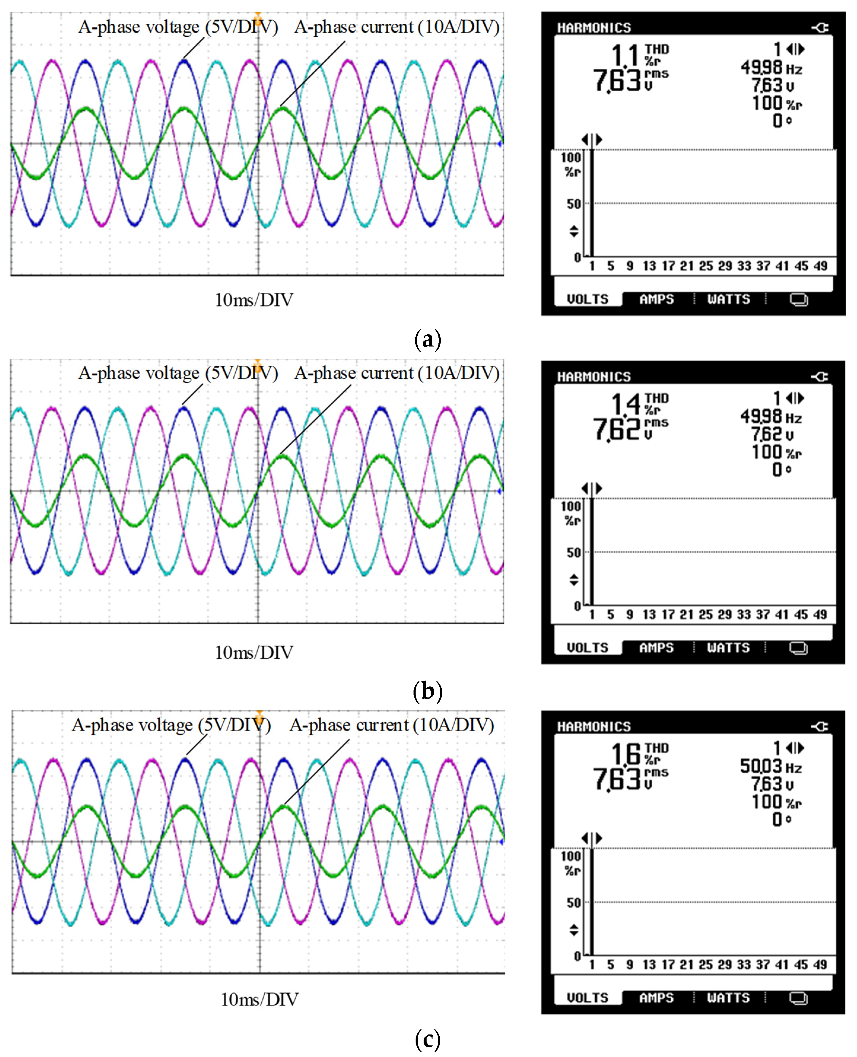
Verification of the applicability of proportional–differential feedforward action in weak grid scenarios. Point D (14.59, 2406.51) in Figure 5 is selected as the most suitable controller parameter in the absence of grid impedance. The parameters for the grid voltage feedforward model were determined in Section 5. Figure 13 presents the current voltage waveforms at the PCC of the grid-connected inverter under Lg = 2 mH, 5 mH, and 10 mH, along with the corresponding spectrograms of the grid-connected currents. Observing the increase in grid impedance, it is evident that the THD value of the grid-connected current at the inverter’s output remains below 5%. This observation underscores the efficacy of the grid voltage feedforward parameter selection scheme proposed in this paper, showcasing enhanced stability of the inverter in weak grid conditions. The method demonstrates a maximum base wave tracking error of 0.65%, indicating its capacity to diminish the steady-state error within the inverter’s grid-connected current.
6.3. Scenario 3
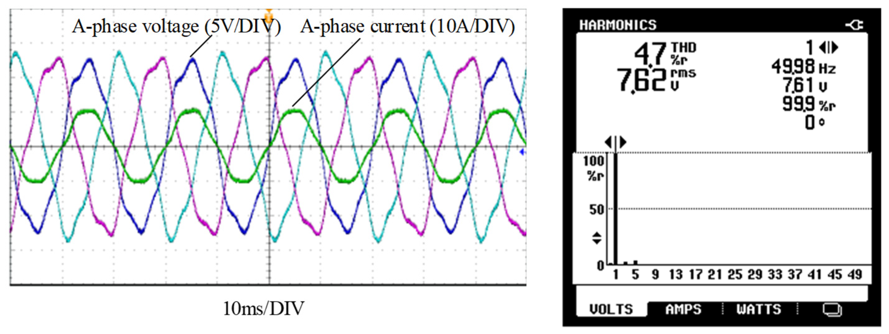
Validation of the grid-connected inverter’s capability to mitigate low-frequency background harmonics within a weak grid environment. Figure 10 illustrates that the grid voltage feedforward amplifies the low-frequency amplitude-frequency characteristics of the inverter’s output impedance Zo(s), resulting in an enhanced harmonic suppression capability within the inverter’s grid-connected current control. Configuring the grid impedance as Lg = 10 mH, the grid voltage source injects 5% of the 3rd harmonic and 5% of the 5th harmonic. The study results, illustrated in Figure 14, indicate that the proposed grid voltage feedforward parameter selection scheme, as presented in this paper, enhances the stability of the inverter during weak grid connections. The observed maximum base wave tracking error of 0.65% illustrates the method’s efficacy in reducing the steady-state error within the inverter’s grid-connected current.
6.4. Scenario 4
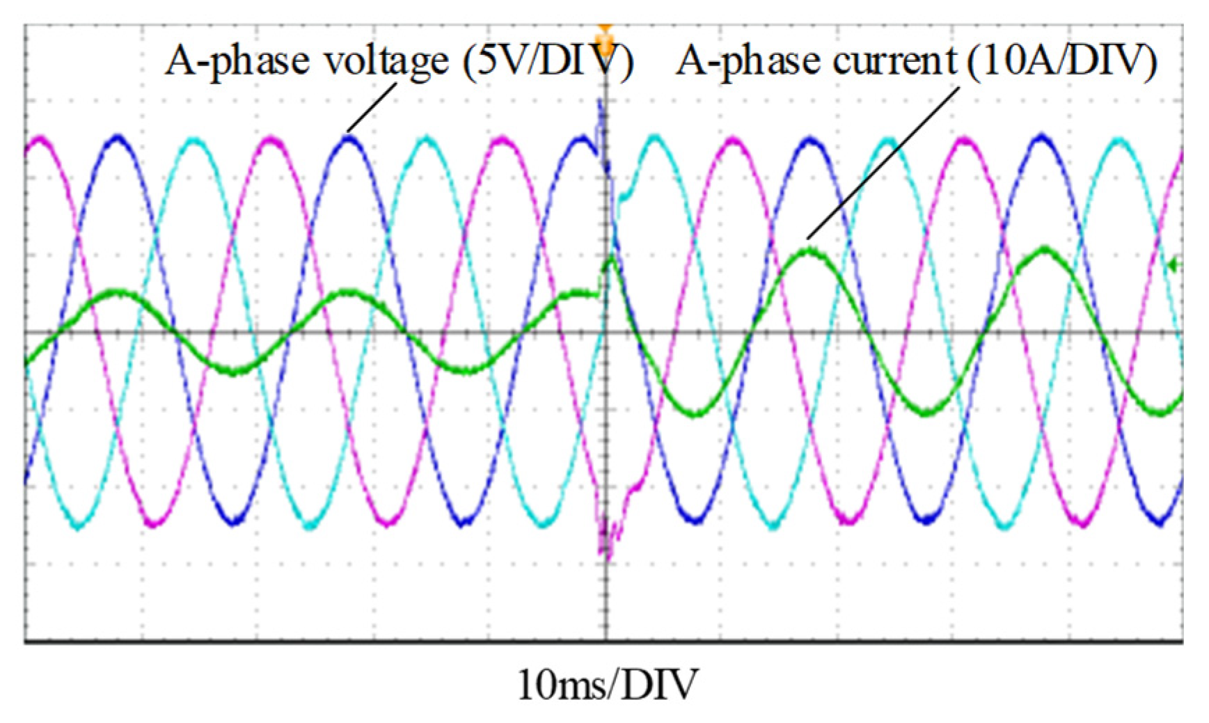
Verification of the dynamic performance of the grid-connected inverter system in a weak grid environment. The grid impedance is configured as Lg = 10 mH, while the grid-connected current command is systematically adjusted from half-load to full-load, illustrated in Figure 15. The grid-connected current demonstrates the capability to adapt to changes in the grid-connected command within half a fundamental frequency cycle, exhibiting minimal overshooting in the current. This observation signifies the commendable dynamic performance of the proposed control strategy.
7. Conclusions and Future Perspectives
In this study, a novel method is proposed, which integrates the D-split method with grid voltage proportional–differential feedforward. The aim is to tackle the issue of amplified grid impedance, typically resulting in resonance within the grid-connected current of the inverter in weak grid scenarios. The method reshapes the output impedance of the inverter, enhancing its adaptability in weak grid scenarios. The following conclusions are derived:
1. The integration of the D-split method with the amplitude-frequency tester facilitates the selection of QPR controller parameters, maximizing the control bandwidth within specified margins. This approach effectively mitigates the loop coupling problem inherent in the synchronous reference system. Such methodological synergy optimizes parameter selection, thereby enhancing overall inverter performance.
2. The amalgamation of the D-split method with the grid voltage feedforward model induces a transformative effect on the inverter’s output impedance. This alteration contributes to heightened stability and robustness, particularly in the face of substantial fluctuations in grid impedance. Furthermore, it enhances the inverter’s ability to reject grid voltage harmonics, signifying an improvement in overall inverter performance under challenging grid conditions.
In this study, we exclusively investigate the application of the D-split method to enhance the stability and robustness of a singular inverter operating within a weak grid. The exploration of utilizing the D-split method for stability and robustness analysis in the context of multiple inverters working in parallel under weak grid conditions remains unexplored. The directions for future research in this domain are outlined as follows:
1. In an array comprising multiple inverters interconnected at a common entry point, the inconsistency in circuit structure parameters arises from the diverse models of the inverters. This disparity gives rise to impedance coupling among the inverters, potentially leading to oscillations in the output current of the inverters. Addressing this challenge involves applying the D-split method to multiple inverters, with the goal of selecting appropriate parameters to mitigate or eliminate the coupling. Resolving this issue constitutes a subject for future investigations.
2. The concurrent operation of multiple inverters introduces errors in the crystal oscillators of each inverter’s digital controller, resulting in unsynchronized control carriers. This asynchrony induces low-frequency oscillations in the power flow among the inverters. A promising avenue for future research involves the application of the D-split method to tackle the challenges associated with power oscillation and carrier desynchronization in the collective operation of multiple inverters.
Author Contributions
Conceptualization, S.W. and G.Z.; methodology, S.W.; software, G.Z.; validation, G.Z.; formal analysis, G.Z.; investigation, G.Z.; resources, P.H.; data curation, J.C.; writing—original draft preparation, G.Z.; writing—review and editing, G.Z.; visualization, P.H.; supervision, S.W.; project administration, S.W.; funding acquisition, P.H. All authors have read and agreed to the published version of the manuscript.
Funding
This work was supported by the Project supported by Key R&D Program of Shaanxi Province, China (2023-YBGY-304) and Department of Education Planning Project of Shaanxi Province (22JC023).
Data Availability Statement
Data are contained within the article.
Conflicts of Interest
The authors declare no conflict of interest.
Abbreviations
The following abbreviations are used in this manuscript:
| THD | Harmonic distortion factor |
| QPR | Quasi–proportional–resonant |
| PLL | Phase-locked loop |
| SPWM | Sinusoidal pulse width modulation |
| SCR | Short circuit impedance ratio |
| HIL | Hardware-in-the-loop |
| PCC | Common grid connection point |
| RT-LAB | Real time laboratory |
References
- Yuan, X.; Zhang, M.; Chi, Y.; Ju, P. Basic Challenges of and Technical Roadmap to Power-electronized Power System Dynamics Issues. Proc. CSEE 2022, 42, 1904–1917. [Google Scholar]
- Chen, X.; Ruan, X.; Yang, D.; Zhao, W.; Jia, L. Injected Grid Current Quality Improvement for a Voltage-Controlled Grid-Connected Inverter. IEEE Trans. Power Electron. 2018, 33, 1247–1258. [Google Scholar] [CrossRef]
- Xie, L.; Zen, S.; Liu, J.; Zhang, Z.; Yao, J. Control and Stability Analysis of the LCL-Type Grid-Connected Converter without Phase-Locked Loop under Weak Grid Conditions. Electronics 2022, 11, 3322. [Google Scholar] [CrossRef]
- Zhu, D.; Zhou, S.; Zou, X.; Kang, Y.; Zou, K. Phase-Locked Loop Small-Signal Disturbance Compensation Control for Three-Phase LCL-Type Grid-Connected Converter under Weak Grid. In Proceedings of the 10th Annual IEEE Energy Conversion Congress and Exposition (ECCE 2018), Portland, OR, USA, 23–27 September 2018; pp. 3108–3112. [Google Scholar]
- Zhang, H.; Ruan, X.; Lin, Z.; Wu, L.; Ding, Y.; Guo, Y. Capacitor Voltage Full Feedback Scheme for LCL-Type Grid-connected Inverter to Suppress Current Distortion Due to Grid Voltage Harmonics. IEEE Trans. Power Electron. 2021, 36, 2996–3006. [Google Scholar] [CrossRef]
- Xu, J.; Xie, S.; Qian, Q.; Zhang, B. Adaptive Feedforward Algorithm Without Grid Impedance Estimation for Inverters to Suppress Grid Current Instabilities and Harmonics Due to Grid Impedance and Grid Voltage Distortion. IEEE Trans. Ind. Electron. 2017, 64, 7574–7586. [Google Scholar] [CrossRef]
- Qian, Q.; Xie, S.; Ji, L.; Xu, J.; Zhang, B. A Current Control Strategy to Improve the Adaptability to Utility for Inverters. Proc. CSEE 2016, 36, 6193–6201. [Google Scholar]
- Wu, X.; Li, X.; Yuan, X.; Geng, Y. Grid Harmonics Suppression Scheme for LCL-Type Grid-Connected Inverters Based on Output Admittance Revision. IEEE Trans. Sustain. Energy 2015, 6, 411–421. [Google Scholar] [CrossRef]
- Akhavan, A.; Vasquez, J.C.; Guerrero, J.M. A Robust Method for Controlling Grid-Connected Inverters in Weak Grids. IEEE Trans. Circuits Syst. II Express Briefs 2021, 46, 1333–1337. [Google Scholar] [CrossRef]
- Zhou, L.; Luo, A.; Chen, Y.; Zhou, X.; Li, M.; Kuang, H. Robust Grid-Connected Current Feedback Active Damping Control Method for LCL Type Grid-Connected Inverter. Proc. CSEE 2016, 36, 2742–2752. [Google Scholar]
- Li, S.; Zhou, S.; Li, H. Harmonic Suppression Strategy of LCL Grid-Connected PV Inverter Based on Adaptive QPR_PV Control. Electronics 2023, 12, 2282. [Google Scholar] [CrossRef]
- Hollweg, G.V.; Bui, V.H.; Silva, F.L.D.; Glatt, R.; Chaturvedi, S.; Su, W. An RMRAC With Deep Symbolic Optimization for DC–AC Converters Under Less-Inertia Power Grids. IEEE Open Access J. Power Energy 2023, 10, 629–642. [Google Scholar] [CrossRef]
- Lu, D.; Wang, X.; Blaabjerg, F. Impedance-Based Analysis of DC-Link Voltage Dynamics in Voltage-Source Converters. IEEE Trans. Ind. Electron. 2019, 34, 3973–3985. [Google Scholar] [CrossRef]
- Wang, C.; Wang, X.; He, Y.; Pan, D.; Zhang, H.; Ruan, X.; Chen, X. Passivity-Oriented Impedance Shaping for LCL-Filtered Grid-Connected Inverters. IEEE Trans. Ind. Electron. 2023, 70, 9078–9090. [Google Scholar] [CrossRef]
- Yang, D.; Ruan, X.; Wu, H. Impedance Shaping of the Grid-Connected Inverter with LCL Filter to Improve Its Adaptability to the Weak Grid Condition. IEEE Trans. Power Electron. 2014, 29, 5795–5805. [Google Scholar] [CrossRef]
- Xie, C.; Li, K.; Zou, J.; Liu, D.; Guerrero, J. Passivity-Based Design of Grid-Side Current-Controlled LCL-Type Grid-Connected Inverters. IEEE Trans. Power Electron. 2020, 35, 9813–9823. [Google Scholar] [CrossRef]
- Hollweg, G.V.; Khan, S.A.; Chaturvedi, S.; Fan, Y.; Wang, M.; Su, W. Grid-Connected Converters: A Brief Survey of Topologies, Output Filters, Current Control, and Weak Grids Operation. Energies 2023, 16, 3611. [Google Scholar] [CrossRef]
- Yan, H.; Cai, H. Research on Fuzzy Active Disturbance Rejection Control of LCL Grid-Connected Inverter Based on Passivity-Based Control in Weak Grid. Electronics 2023, 12, 1847. [Google Scholar] [CrossRef]
- Chen, W.; Zhao, J.; Liu, K.; Cao, W. Passivity enhancement for LCL-filtered grid-connected inverters using the dominant-admittance-based controller. IET Power Electron. 2020, 13, 4140–4149. [Google Scholar] [CrossRef]
- Wang, X.; Qin, K.; Ruan, X.; Pan, D.; He, Y.; Liu, F. A robust grid-voltage feedforward scheme to improve adaptability of grid-connected inverter to weak grid condition. IEEE Trans. Power Electron. 2021, 36, 2384–2395. [Google Scholar] [CrossRef]
- Wang, X.; Liu, Y.; Zhang, X.; Yang, Q.; Zhang, C. Research on Novel Control Strategy for Grid-Connected Inverter Suitable for Wide-Range Grid Impedance Variation. Electronics 2020, 9, 623. [Google Scholar] [CrossRef]
- Wang, J.; Yan, J.; Jiang, L.; Zou, J. Delay-Dependent Stability of Single-Loop Controlled Grid-Connected Inverters with LCL Filters. IEEE Trans. Power Electron. 2016, 31, 743–757. [Google Scholar] [CrossRef]
- Zhang, X.; Chen, W.; Wang, G.; Xu, D. A Symmetrical Control Method for Grid-Connected Converters to Suppress the Frequency Coupling Under Weak Grid Conditions. IEEE Trans. Power Electron. 2020, 35, 13488–13499. [Google Scholar] [CrossRef]
- Hwang, C.; Hwang, L.; Hwang, J. Robust D-partition. J. Chin. Inst. Eng. 2010, 33, 811–821. [Google Scholar] [CrossRef]
- Liu, J.; Xue, Y.; Li, D. Calculation of PI controller stable region based on D-partition method. In Proceedings of the International Conference on Control, Automation and Systems (ICCAS), Gyeonggi-do, Republic of Korea, 12–15 October 2010; pp. 2185–2189. [Google Scholar]
- Xie, C.; Li, K.; Zou, J.; Guerrero, J. Passivity-Based Stabilization of LCL-Type Grid-Connected Inverters via a General Admittance Model. IEEE Trans. Power Electron. 2020, 35, 6636–6648. [Google Scholar] [CrossRef]
- Liu, B.; Wei, Q.; Zou, C.; Duan, S. Stability Analysis of LCL-Type Grid-Connected Inverter Under Single-Loop Inverter Side Current Control with Capacitor Voltage Feedforward. IEEE Trans. Ind. Inf. 2018, 14, 691–702. [Google Scholar] [CrossRef]
- Dannehl, J.; Fuchs, F.; Thogersen, P. PI state space current control of grid-connected PWM converters with LCL filters. IEEE Trans. Power Electron. 2010, 25, 2320–2330. [Google Scholar] [CrossRef]
- Gabe, I.; Montagner, V.; Pinheiro, H. Design and implementation of a robust current controller for VSI connected to the grid through an LCL filter. IEEE Trans. Power Electron. 2009, 24, 1444–1452. [Google Scholar] [CrossRef]
- Sun, J. Impedance-Based Stability Criterion for Grid-Connected Inverters. IEEE Trans. Power Electron. 2011, 26, 3075–3078. [Google Scholar] [CrossRef]
- Alenius, H.; Luhtala, R.; Messo, T.; Roinila, T. Autonomous reactive power support for smart photovoltaic inverter based on real-time grid-impedance measurements of a weak grid T. Electr. Power Syst. Res. 2020, 182, 106207. [Google Scholar] [CrossRef]
- Chowdhury, V.R.; Kimball, J.W. Grid Voltage Estimation and Feedback Linearization based Control of a Three phase Grid Connected Inverter under Unbalanced Grid Conditions with LCL Filter. In Proceedings of the IEEE Energy Conversion Congress and Exposition, ECCE, Baltimore, MD, USA, 29 September–3 October 2019; pp. 2979–2984. [Google Scholar]
- Wu, G.; Wang, X.; He, Y.; Ruan, X.; Zhang, H. Inductor-Current Proportional-Derivative Feedback Active Damping for Voltage-Controlled VSCs. In Proceedings of the IEEE 12th Energy Conversion Congress & Exposition—Asia (ECCE—Asia), Singapore, 24–27 May 2021; pp. 2357–2362. [Google Scholar]
Figure 1.
System structure of the LCL-filtered grid-connected inverter.

Figure 2.
Control block diagrams of an LCL-filtered grid-connected inverter without voltage feedforward.
Figure 2.
Control block diagrams of an LCL-filtered grid-connected inverter without voltage feedforward.

Figure 3.
Amplitude–phase margin analysis tester.

Figure 4.
Establishing controller parameters using the D-split method. (a) Region of controller parameter stabilization, (b) Bode plot of Go(s) under critical stabilization controller parameters (Letters A and B denote the Bode plots of the open-loop transfer functions corresponding to the points in (a)).

Figure 5.
Determination of controller parameters from the D-split method. (a) Controller Stabilization Parameter Domains under Multi-Objective, (b) Bode plot of controller parameters with margins included (Letters C, D, F, and G denote the Bode plot of the open-loop transfer function corresponding to the respective points in (a)).

Figure 6.
Analyzing the bandwidth information of parameters within the shaded region illustrated in Figure 5a.
Figure 6.
Analyzing the bandwidth information of parameters within the shaded region illustrated in Figure 5a.

Figure 7.
Norton equivalent circuit modeling for inverters in weak grid conditions.

Figure 8.
Control block diagrams of LCL-filtered grid-connected inverter with voltage feedforward.

Figure 9.
Stable region of voltage feedforward proportional and differential coefficients in relation to varying grid impedances.
Figure 9.
Stable region of voltage feedforward proportional and differential coefficients in relation to varying grid impedances.

Figure 10.
Frequency response comparison of inverter output and grid impedance without grid voltage feedforward and with proportional–differential feedforward.
Figure 10.
Frequency response comparison of inverter output and grid impedance without grid voltage feedforward and with proportional–differential feedforward.

Figure 11.
Photograph of HIL prototype. (a) Photographs of the HIL setup, (b) schematic of the HIL structure.
Figure 11.
Photograph of HIL prototype. (a) Photographs of the HIL setup, (b) schematic of the HIL structure.

Figure 12.
HIL simulation waveforms of grid-connected current without grid impedance. (a) Influence of a-point controller parameters, (b) influence of b-point controller parameters. (Lime green curve: B-phase voltage; Pink curve: C-phase voltage).
Figure 12.
HIL simulation waveforms of grid-connected current without grid impedance. (a) Influence of a-point controller parameters, (b) influence of b-point controller parameters. (Lime green curve: B-phase voltage; Pink curve: C-phase voltage).

Figure 13.
HIL simulation waveforms of grid-connected current and its THD analysis under various grid impedances. (a) Lg = 2 mH, (b) Lg = 5 mH, (c) Lg = 10 mH. (Lime green curve: B-phase voltage; Pink curve: C-phase voltage).
Figure 13.
HIL simulation waveforms of grid-connected current and its THD analysis under various grid impedances. (a) Lg = 2 mH, (b) Lg = 5 mH, (c) Lg = 10 mH. (Lime green curve: B-phase voltage; Pink curve: C-phase voltage).

Figure 14.
HIL simulation waveforms of grid-connected current in the presence of voltage harmonics within a weak grid. (Lime green curve: B-phase voltage; Pink curve: C-phase voltage).
Figure 14.
HIL simulation waveforms of grid-connected current in the presence of voltage harmonics within a weak grid. (Lime green curve: B-phase voltage; Pink curve: C-phase voltage).

Figure 15.
HIL simulation waveforms displaying the dynamic response of grid-connected current. (Lime green curve: B-phase voltage; Pink curve: C-phase voltage).
Figure 15.
HIL simulation waveforms displaying the dynamic response of grid-connected current. (Lime green curve: B-phase voltage; Pink curve: C-phase voltage).


Table 1.
Parameters of the HIL simulation model.
| Symbol | Instruction | Values |
|---|---|---|
| Uo | Grid voltage | 220 V |
| fn | Grid frequency | 50 Hz |
| Pn | Rated power | 5 kW |
| In | Rated current | 7.57 A |
| Ts | Sample time | 100 us |
| fs | Switching frequency | 10 kHz |
| L1 | Inverter inductance | 4.2 mH |
| Cf | Filter capacitor | 5 uF |
| L2 | Grid-side inductance | 1.2 mH |
| Udc | DC voltage | 700 V |
Disclaimer/Publisher’s Note: The statements, opinions and data contained in all publications are solely those of the individual author(s) and contributor(s) and not of MDPI and/or the editor(s). MDPI and/or the editor(s) disclaim responsibility for any injury to people or property resulting from any ideas, methods, instructions or products referred to in the content. |
© 2023 by the authors. Licensee MDPI, Basel, Switzerland. This article is an open access article distributed under the terms and conditions of the Creative Commons Attribution (CC BY) license (https://creativecommons.org/licenses/by/4.0/).
Share and Cite
MDPI and ACS Style
Wang, S.; Zhou, G.; Hao, P.; Chen, J. Designing Parameters to Reshape the Inverter Output Impedance Based on the D-Split Method under Weak Grid Conditions. Electronics 2023, 12, 5000. https://doi.org/10.3390/electronics12245000
AMA Style
Wang S, Zhou G, Hao P, Chen J. Designing Parameters to Reshape the Inverter Output Impedance Based on the D-Split Method under Weak Grid Conditions. Electronics. 2023; 12(24):5000. https://doi.org/10.3390/electronics12245000
Chicago/Turabian StyleWang, Su’e, Guangyuan Zhou, Pengfei Hao, and Jingwen Chen. 2023. "Designing Parameters to Reshape the Inverter Output Impedance Based on the D-Split Method under Weak Grid Conditions" Electronics 12, no. 24: 5000. https://doi.org/10.3390/electronics12245000
Note that from the first issue of 2016, this journal uses article numbers instead of page numbers. See further details here.