
Arc_EffNet: A Novel Series Arc Fault Detection Method Based on Lightweight Neural Network
by
 , ,
, ,
Xin Ning
1,2,
Dejie Sheng
3,*,
Jiawang Zhou
3,
Yuying Liu
3,
Yao Wang
3 ,
,
Hua Zhang
1,2 and
Xiao Lei
1,2 1
State Grid Sichuan Electric Power Research Institute, Chengdu 610041, China
2
Power Internet of Things Key Laboratory of Sichuan Province, Chengdu 610041, China
3
School of Electrical Engineering, Hebei University of Technology, Tianjin 300400, China
*
Author to whom correspondence should be addressed.
Electronics 2023, 12(22), 4617; https://doi.org/10.3390/electronics12224617
Submission received: 13 October 2023
/
Revised: 8 November 2023
/
Accepted: 9 November 2023
/
Published: 11 November 2023
(This article belongs to the Section Industrial Electronics)
Abstract
:Arc faults can cause a severe electric fire, especially series arc faults. Artificial intelligence (AI)-based arc fault detection methods can have a boasted detection accuracy. However, the complexity and large parameter quantity of the AI-based algorithm will hinder its real-time performance for detecting series arc faults. This paper proposes a lightweight arc fault detection method based on the EffNet module, which can make the algorithm less complex with the same detection accuracy level. An arc fault test platform was constructed to collect arc current data, covering eight types of loads required by the IEC 62606 standard. The raw arc current data are used directly as an input for the proposed algorithm, reducing the module’s complexity. According to features of arc current mainly represented in the time domain, the first and last convolution layers of the EffNet module can be improved. Additionally, the spatially separable convolution is well-tuned and trimmed to achieve a more lightweight and better-performance architecture for arc fault detection called Arc_EffNet. Remarkably, this model achieves an impressive arc detection accuracy of 99.75%. An arc fault detection prototype was built using the Raspberry Pi 4B to evaluate the real-time detecting performance of the proposed method. The experimental results show that the prototype takes a time of about 72 ms to respond to a series arc fault, which can fulfill the requirement of real-time detection for arc faults.
1. Introduction
Electrical fire accidents brought on by faulty electrical equipment and aging electrical lines are rising year-over-year along with the constant rise in power usage [1]. A total of 220,000 electrical fires broke out in China in 2021 [2], more than 60% of which were brought on by arc faults in medium- and low-voltage systems. In more than three out of every five fires (63%) involving an electrical failure or malfunction in homes from 2015 to 2019 [3], arcing was the heat source. IEC 62606-2017, which specifies the general specifications of arc fault detection device (AFDD) [4], was amended and published in 2017 by the International Electrotechnical Commission (IEC). According to the standard, AFDD’s maximum rated voltage and current can now be up to 240 V/63 A. A significant portion of the low-voltage distribution system’s loads are nonlinear, and a significant portion of its normal working current is made up of high-order harmonics. Because of the distortion, the waveform can no longer be classified as a sine wave [5,6]. The load features have a significant impact on the series arc fault current waveform, and because of their complexity and concealment, they pose significant fire threats to the low voltage distribution system [7]. The traditional series arc fault detection approach, which is simple to use on an embedded platform, establishes the feature threshold to recognize the arc fault by human experience. The authors in [8] devised an arc fault detection approach based on their research on the symmetrical energy distribution of arc fault voltage. However, it is typically challenging to obtain the arc voltage waveform in the actual line. The current research focuses on the arc current signal since it is simpler to gather and analyze. The authors in [9] identified the series arc fault by comparing the difference of the arc current’s high-frequency signals to the detection threshold. The authors in [10] extracted the high-frequency detail feature value of the arc current using wavelet transform, and the arc fault was identified using this information. However, the fixed feature threshold finds it challenging to accurately identify the arc fault under a variety of working conditions in power lines with numerous nonlinear loads due to the interference of high-frequency harmonics, and the conventional detection method will result in protection miss-operation. The authors in [11] used an improved spectral subtraction to achieve the real-time noise reduction of current signals required by the arc fault detection algorithm. Protection rejection could result from raising the barrier in order to prevent miss-operation. The traditional arc fault circuit interrupter (AFCI) only has an action accuracy of roughly 60% [12]. A new approach for arc fault detection is offered by the advancement of artificial intelligence technology [13,14,15]. In contrast to the conventional approach, the convolutional neural network-based arc fault detection model has excellent accuracy and reliability and can automatically extract the features of arc fault. Reference [16] provided an arc fault detection model based on a convolutional neural network, which enabled the real-time processing and state recognition of current data. The authors in [17] constructed a convolutional neural network with time domain visualization. As the network input, the half-wave arc current signal was translated into a grayscale image, and the network model was trained to recognize the arc fault. Sparse coding is utilized in [18] to collect signal features, and a sparse representation and fully connected neural network (SRFCNN) is created for feature learning and classification, which can avoid the nonlinear load start-up miss-operation. The artificial intelligence-based arc fault detection methods outperform existing methods in terms of identification accuracy [19]. However, the neural network model has a complex structure and a high number of parameters, and it takes a lot of storage space and computer resources. It is challenging to implement the neural network model on an embedded platform, and it cannot match the real-time arc detection criteria. In [20], a shallow DNN network for arc fault detection was constructed, which can detect arc faults under simple operating settings while meeting real-time requirements. However, the shallow DNN network topology has inadequate representation, making it inappropriate for arc defect detection in complex operating circumstances.
There are currently few studies on the detection method of series arc faults for lightweight neural networks, and no well-developed detection method for AC series arc fault exists. As a result, studying an arc fault detection model based on lightweight neural network, enhancing its accuracy and reliability, and lowering the number of its network parameters and its level of calculations are of considerable theoretical importance and have extensive application potential.
The lightweight detection method of series arc fault is chosen as the research objective of this work. The EffNet-based arc fault detection model is constructed. Finally, the arc fault detection device is built on the Raspberry Pi platform. This paper’s primary research contents are as follows:
- To collect the arc fault current, a series arc fault test platform is constructed. It is split into four groups based on the operating principle of the load, and the time and frequency domain features of the arc current of various types of loads are investigated. Data were collected using the test platform and a series arc fault dataset was created.
- We improved the traditional EffNet network structure and constructed an Arc_EffNet arc fault detection model. The learning rate update strategy and the automatic stop training strategy are designed to keep the model from falling into the local optimal solution and from overfitting. The results of the experiment reveal that the Arc_EffNet model has a detection accuracy of 99.75%.
- The advantages and disadvantages of various embedded platforms are analyzed for deciding on the Raspberry Pi 4B platform for building an arc fault detecting device. The Arc_EffNet model is performed using the Raspberry Pi platform, and the arc fault detection algorithm is designed to detect series arc faults. Experiments are used to validate the detecting device’s performance in accordance with the IEC 62606 standard.
2. Data Collection and Analysis
2.1. Arc Fault Test Platform
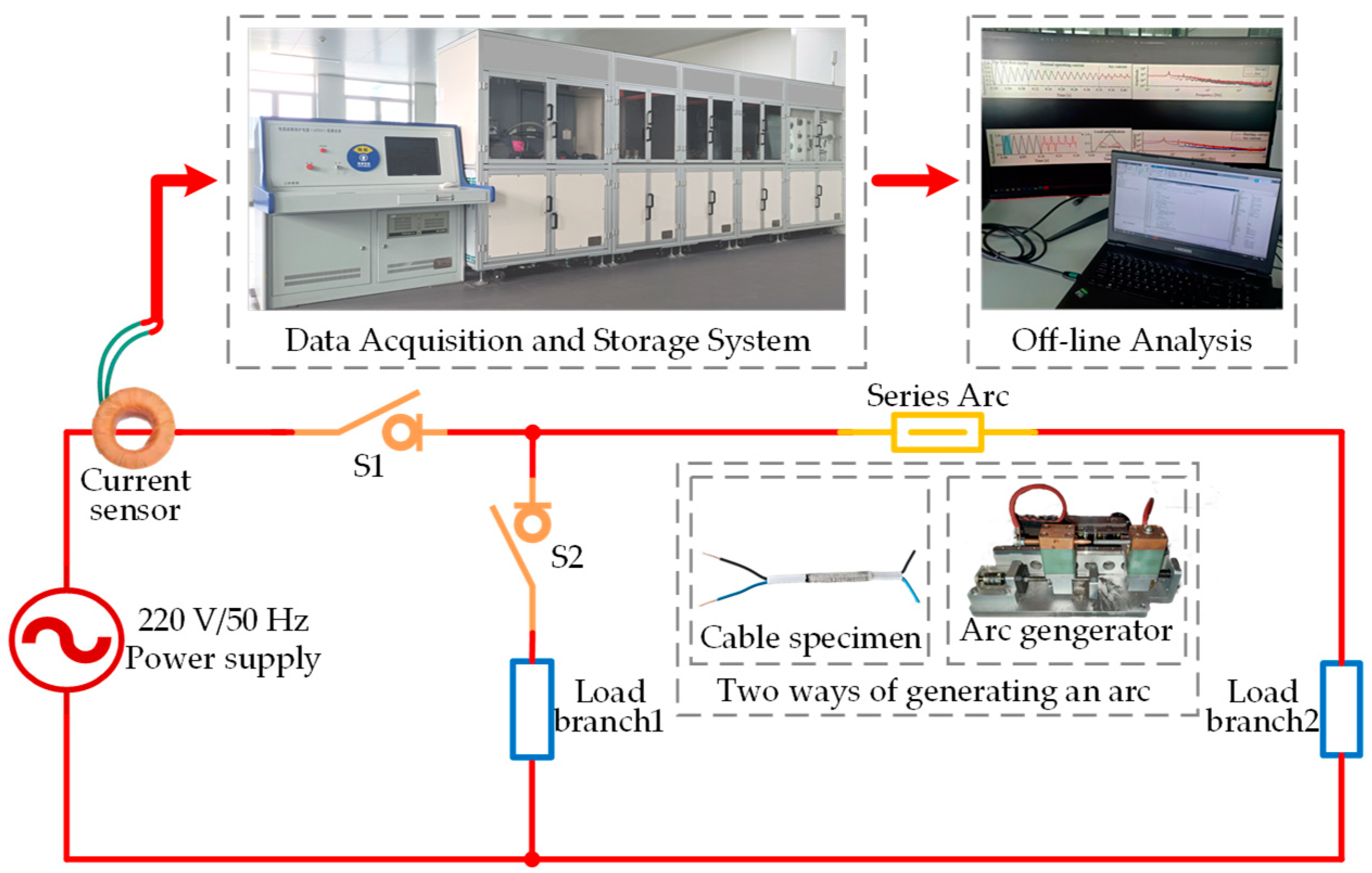
The series arc fault detection research necessitates a large amount of data; however, collecting the actual fault arc current is difficult. A series arc fault test platform has been built in accordance with the IEC 62606 standard, as shown in Figure 1. The platform can replicate arc faults caused by inadequate contact and insulation aging under a variety of working situations. It includes a 220 V and 50 Hz power supply, two load branches, a data capture and storage system, and an arc generator. The arc generator can generate two kinds of arcs: point contact and carbonization path. The arc generator can simulate arcs produced by loose wire terminal connections in actual scenarios, while carbonized cables can simulate arcs produced by damaged wire insulation in actual scenarios. In order to simulate different combinations of experimental loads, a load branch control switch S2 is set in the circuit. The test current signal is collected through the current sensor and transmitted to the data acquisition system for display and storage, and a computer is used for the offline analysis of the data.
The experiment’s data can be recorded by the data capture and storage system. According to the study in Reference [21], the frequency domain features of a series arc fault are most visible in the frequency range of 3 kHz to 20 kHz. The sample rate for A/D is 100 kS/s.
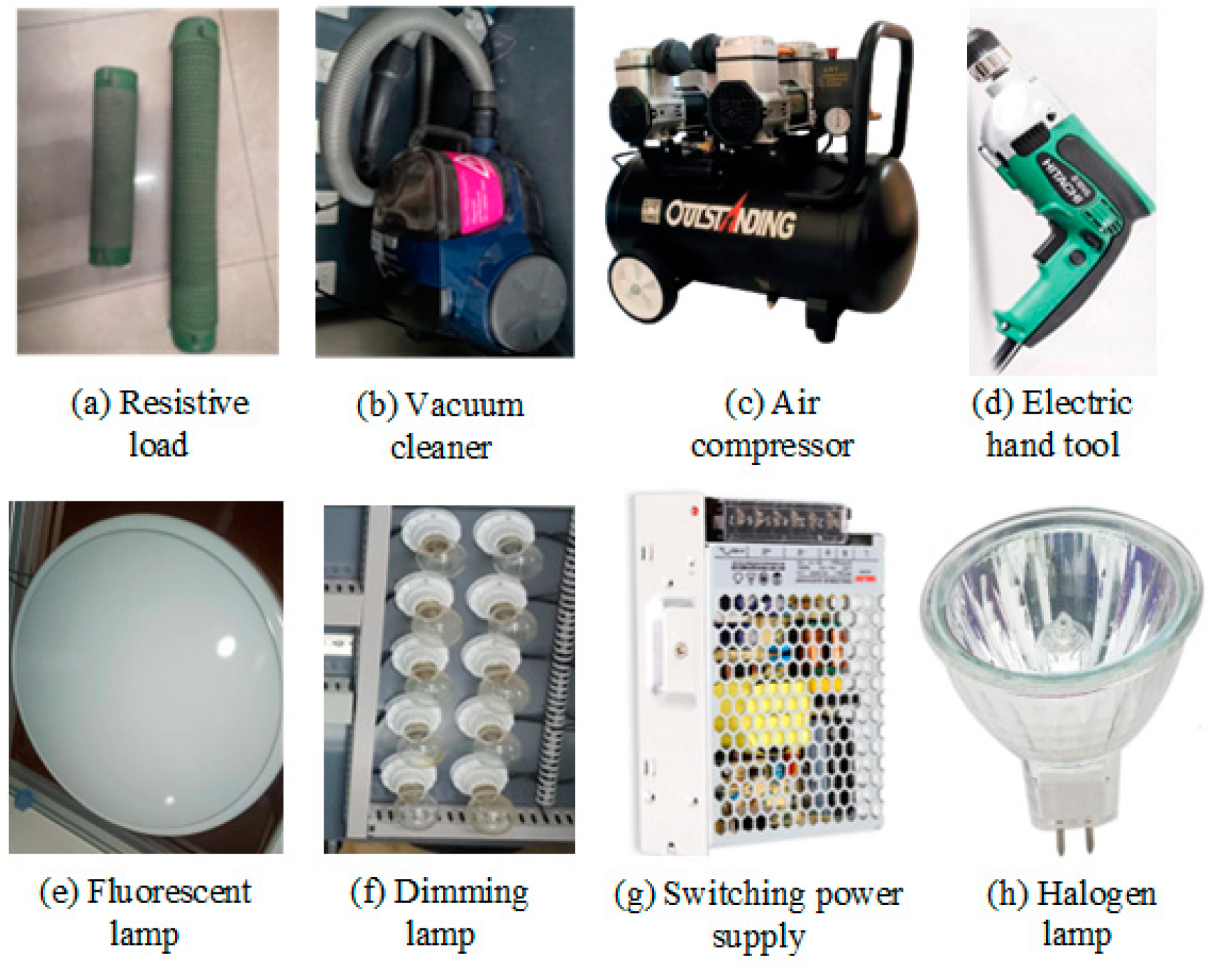
The IEC 62606 standard specifies eight different types of loads for testing, as shown in Table 1. The tests include series arc fault tests and masking tests. Series arc fault tests use a resistor as the test load. Other loads are included in the masking tests.
2.2. Analysis of Arc Fault Current Features
As previously stated, the arc current is the foundation for detecting arc faults. The linearity of the resistive load contributes to an improved accuracy of arc fault detection. Detecting the arc fault current in nonlinear loads is difficult since their normal operating current has time and frequency domain features comparable to the arc current. They are split into four distinct groups based on the working features of the load utilized in the tests, as shown in Table 1.
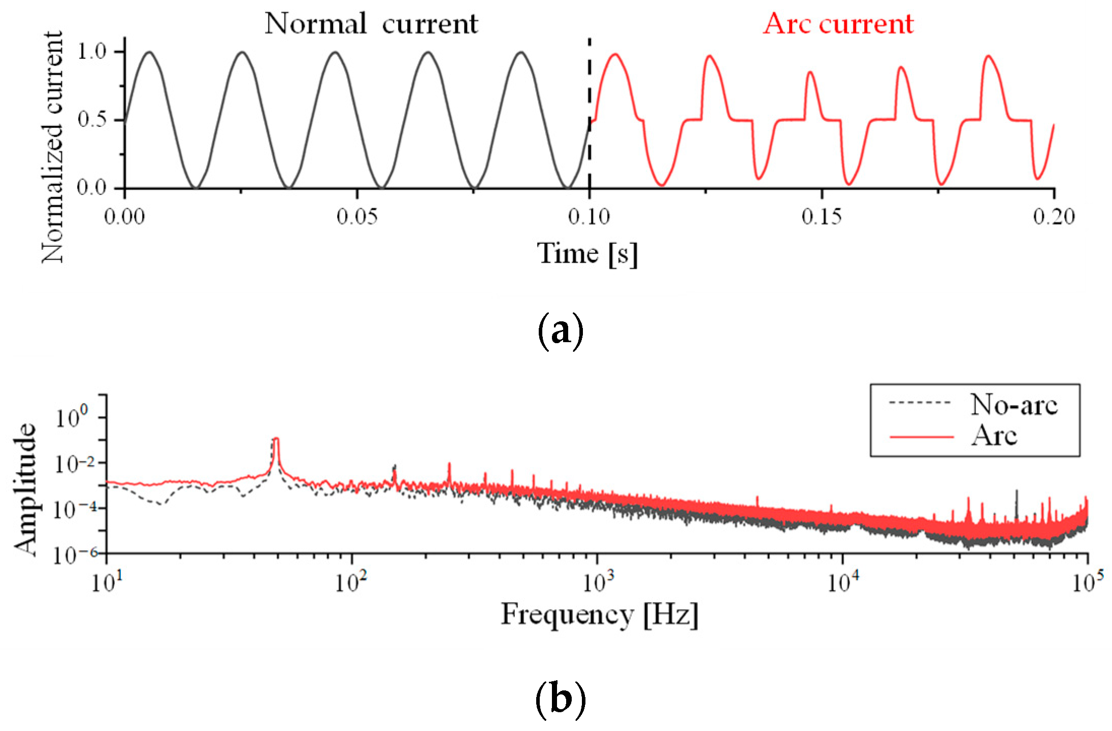
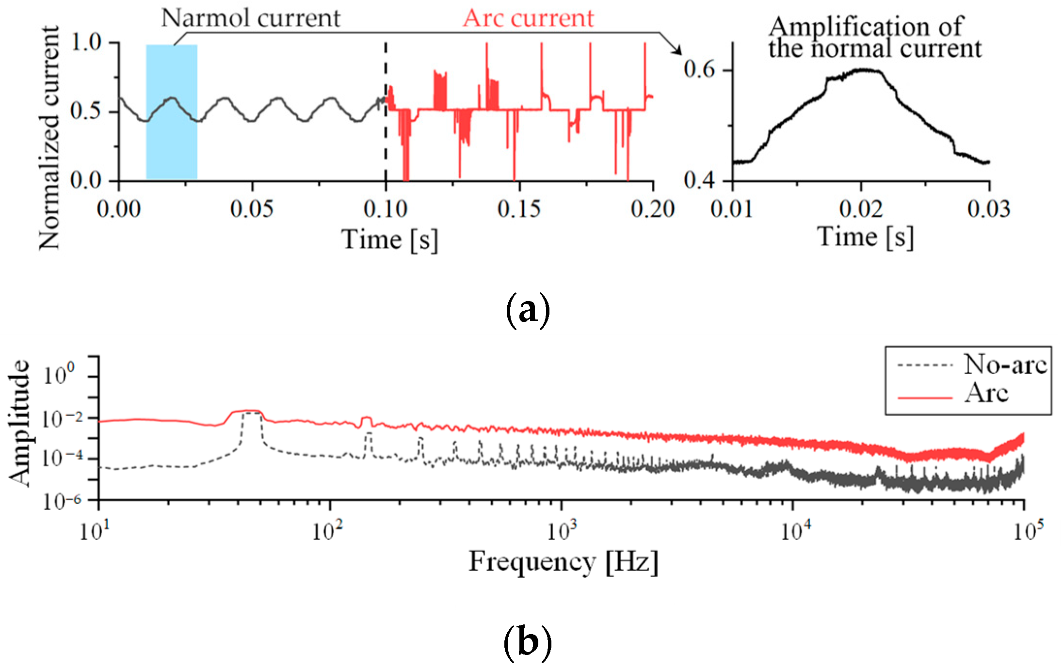
The linear load’s usual working current is a power frequency sine wave with a small high-frequency harmonic component. The time domain waveform and spectrogram of resistive load current are shown in Figure 2. The spectrogram does not change considerably when an arc fault occurs; however, the time domain waveform clearly shows arc features. The arc fault occurs at 0.1 s. The arc is analogous to a variable resistance. The effective value of the current drops when an arc fault occurs. The ‘flat shoulder’ of the arc current appears. The similarity of consecutive periods of arc current will also decrease greatly due to the instability of arc combustion.
The spectrum of arc current is shown in Figure 2b. The amplitude of normal working current and arc current in the frequency domain is similar in the frequency range of 50–100 kHz. Several peaks in the spectrogram amplitude of arc fault current arise between 100 Hz–1 kHz and 20 kHz–80 kHz. However, in the spectrogram, the fault arc current and the normal operating current almost overlap, making the direct arc fault detection impossible.
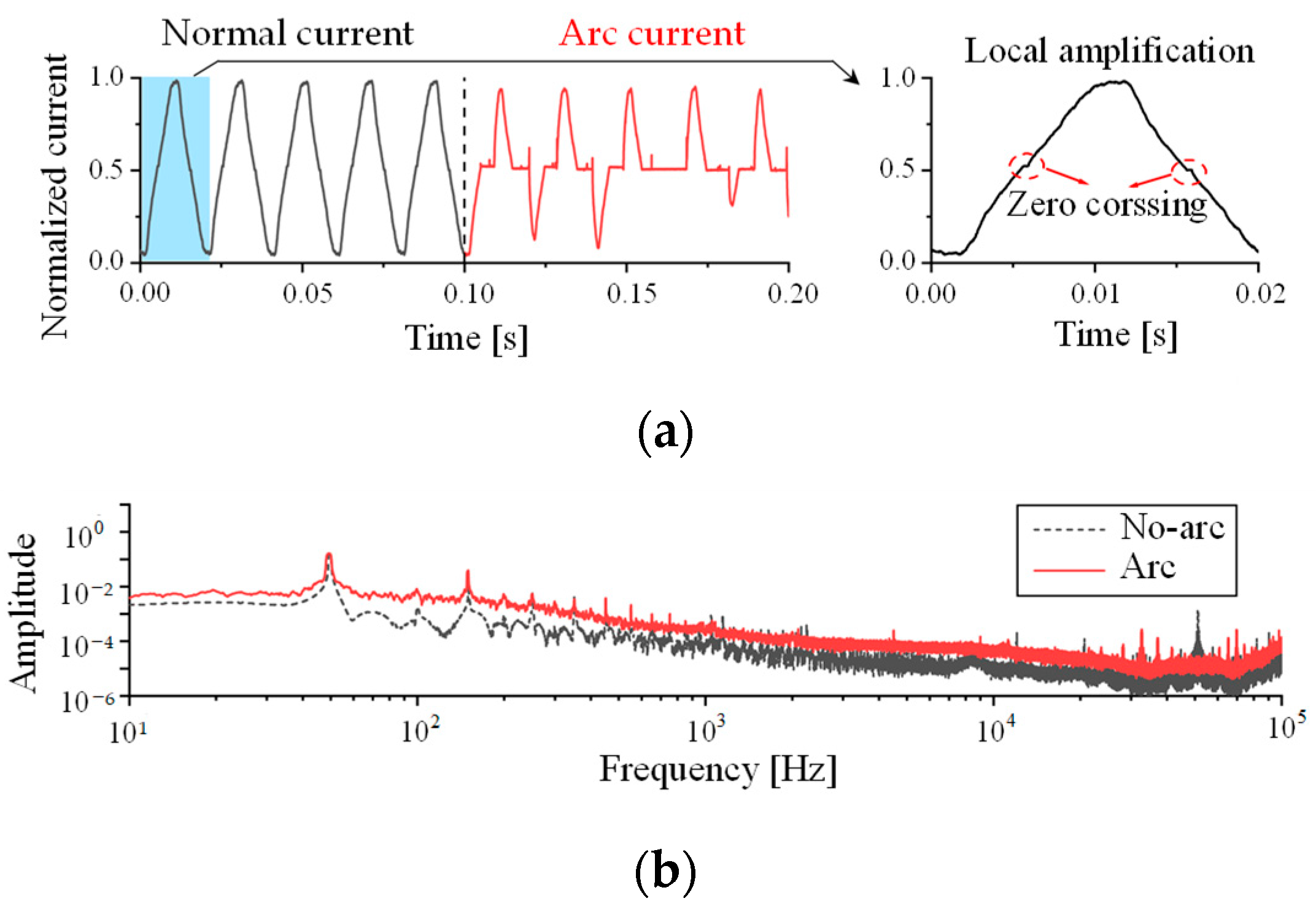
The time domain waveform of the vacuum cleaner load Is shown In Figure 3a. The waveform has multiple spikes due to an increase in high-frequency harmonics. The half-wave vanished after 0.15 s due to the instability of the arcing. The typical working current of the motor load will also appear as ‘zero crossing’ similar to the arc current, as indicated in Figure 3a’s upper right magnification diagram, due to the motor’s commutation and other factors. However, the normal current remains a stationary signal, and its parameters, such as effective value and current similarity, do not alter considerably. The spectrogram is shown in Figure 3b. However, because of the high-order harmonics in the vacuum cleaner’s working current, there are many overlapping areas in the spectrogram between the operating current and the arc current.
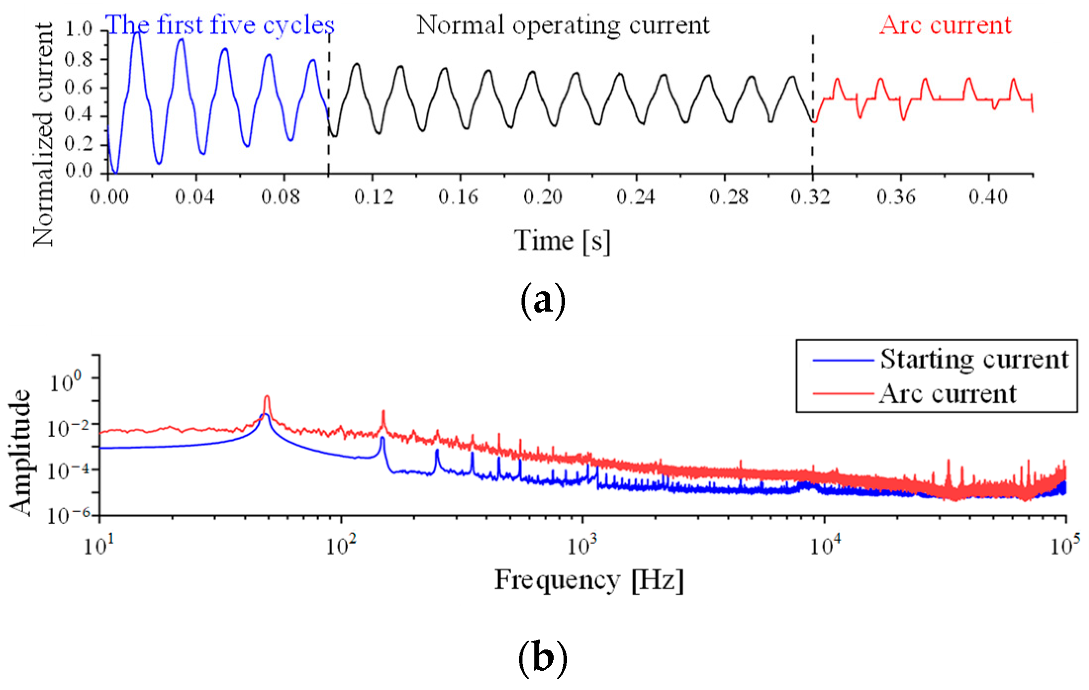
The starting current of the vacuum cleaner is 2–3 times the rated current, as shown in Figure 4a, and the current steadily decreases during the starting process, similar to how the arc fault current drops. The spectrogram is seen in Figure 4b. The spectrogram amplitudes of starting current and arc current are clearly distinguished below 8 kHz, but significantly overlap above 10 kHz.
The gas discharge load works on the principle of gas discharge, necessitating it to be connected to the ballast in order to function, and the working current contains many high-order harmonics. The time-domain waveform of fluorescent lamp load is shown in Figure 5a. The fluorescent lamp’s normal functioning current waveform features a ‘zero crossing’, which is similar to that of the arc fault current. There is a high-frequency harmonic component, and the front and back half-waves of the waveform are asymmetric. The normal working current is very steady, the current similarity between the front and rear cycles is high, and the effective value of the current does not vary substantially. After an arc fault occurs, the ‘zero crossing’ develops, along with the high-frequency harmonics, and the symmetry and similarity of the current waveform decrease dramatically. The spectrogram is depicted in Figure 5b. Arc current has a higher spectrogram amplitude than that of the normal working current. Normal working current has multiple harmonic components and amplitude spikes in the 100 Hz–4 kHz and 30 kHz–80 kHz ranges.
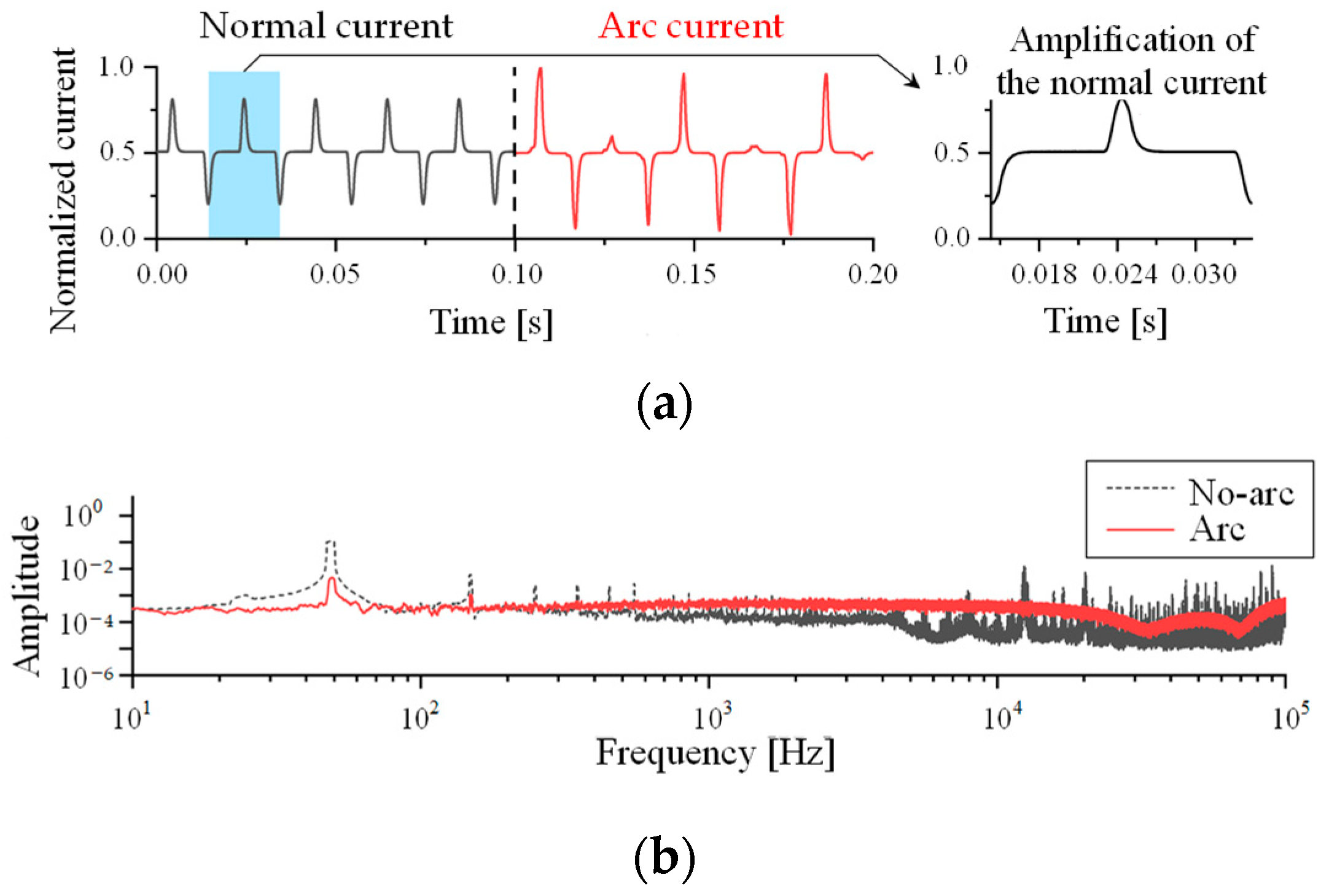
Power electronic load operates primarily by using PWM technology to manage the power electronic devices such as MOSFETs. The time-domain waveform is shown in Figure 6a. There is a visible ‘flat shoulder’ part in the switching power supply’s normal working current, which is similar to the arc current’s ‘zero crossing’ feature. When an arc fault occurs, the current waveform shows obvious asymmetry, similarity decreases, and current waveform distortion is visible. The spectrogram shown in Figure 6b. There are multiple spikes in the spectrogram of the normal current in the frequency ranges of 100 Hz–1 kHz and 10 kHz–100 kHz. In the spectrogram, there are numerous overlapping areas between the normal current and the arc fault current.
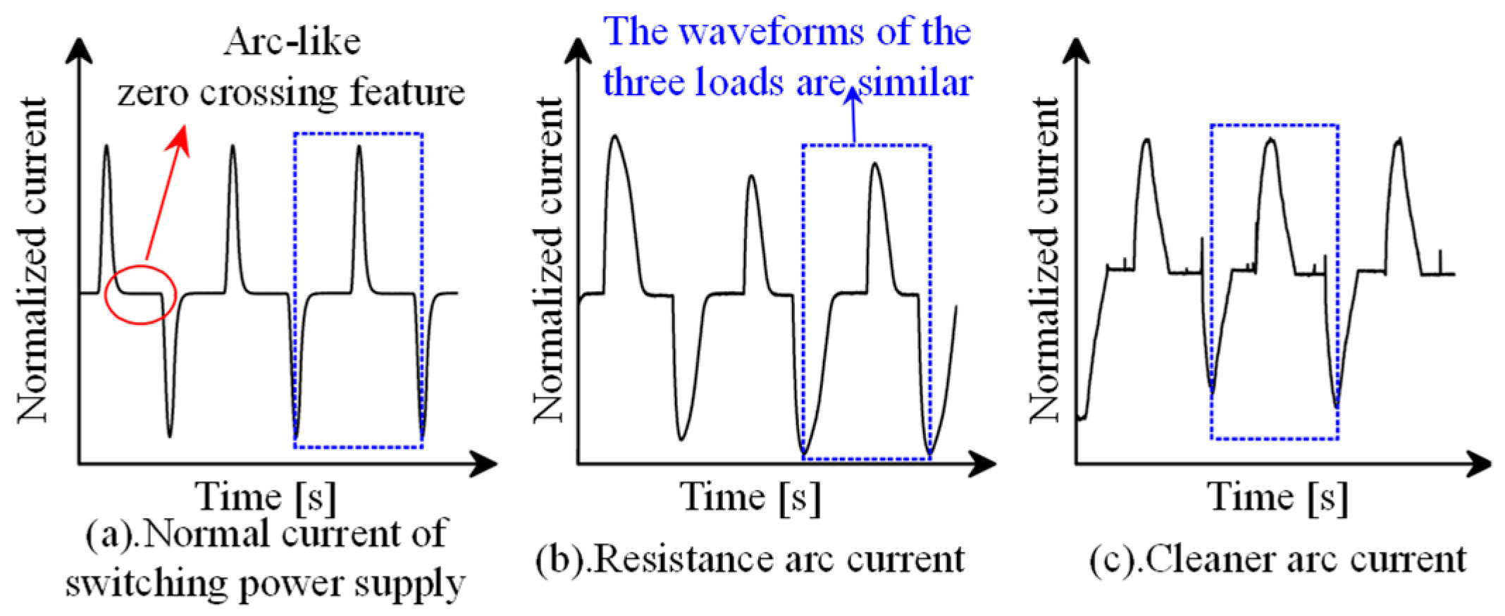
When all types of loads are evaluated independently in the time domain, the time domain features of the arc fault current are clear. The normal current of the switching power supply is comparable to the current when the resistance and the vacuum cleaner have an arc fault, as shown in Figure 7, and it is difficult to differentiate between them merely by relying on time domain features. The normal current and arc current of each load overlap in the spectrogram, and the amplitude of the spectrogram varies. It is difficult to identify an arc fault with a consistent threshold.
It is challenging to choose the arc fault detection method’s threshold based on the time–frequency domain properties of the arc current. It is prone to miss-operation and rejection. Convolutional neural networks can be used to extract arc features and enhance their accuracy and reliability when using artificial intelligence technologies to detect arc faults. Because the neural network can extract high-dimensional features from the input signal, the raw arc current signal can be used for research on the lightweight detection method based on artificial intelligence, which not only eliminates the influence of human factors but also eliminates the complex signal process of the raw current and saves calculation steps.
3. Lightweight Technology of Convolutional Neural Network
3.1. Convolutional Neural Network and Lightweight Method
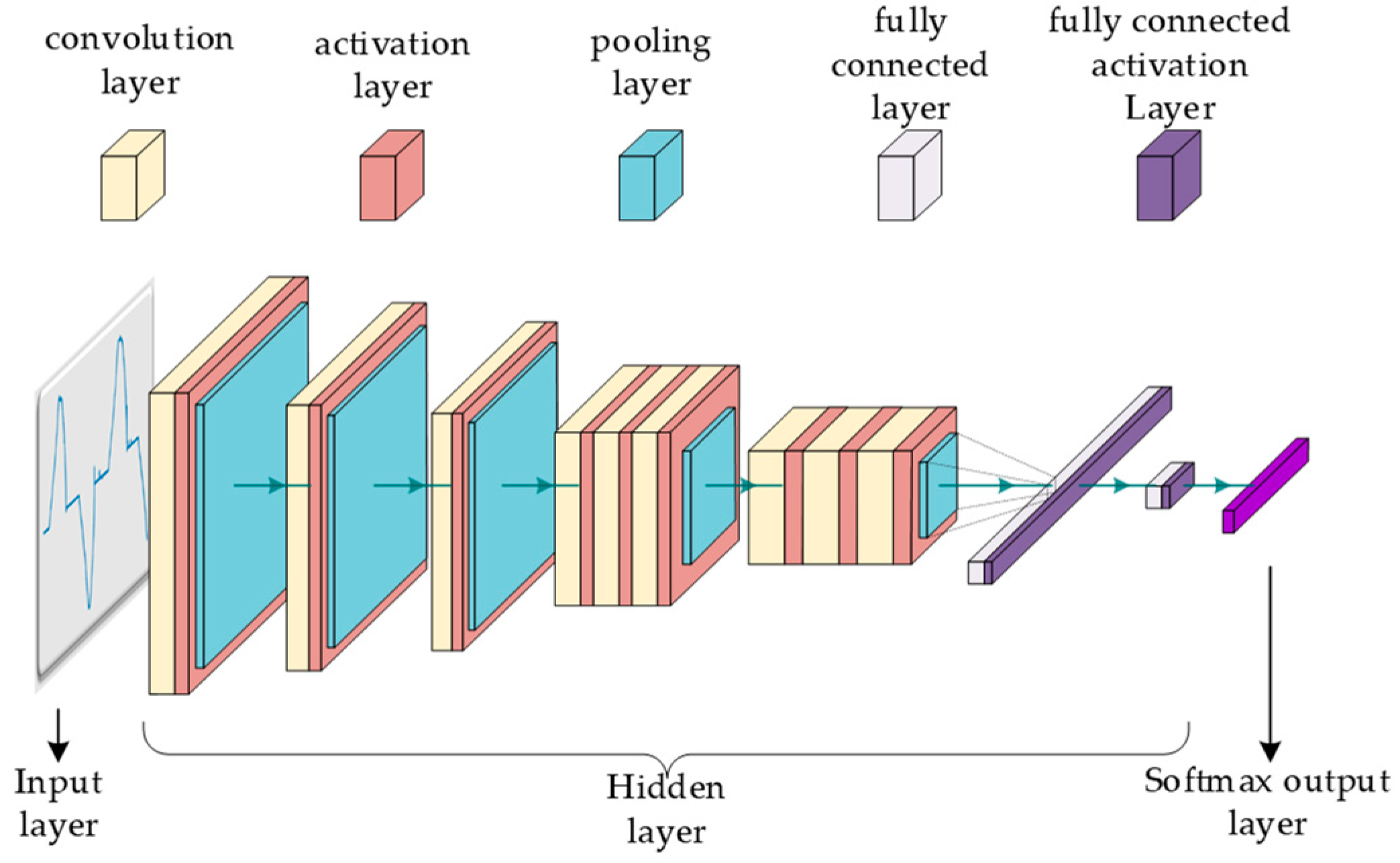
Artificial intelligence approaches are frequently used in industries such as fault detection, machine vision, automatic driving, and others. In contrast to traditional methods, artificial intelligence technologies can automatically extract the features of input data and have a high degree of generalization. CNN is a well-known artificial intelligence algorithm. Figure 8 depicts the traditional CNN structure.
CNN feature extraction relies heavily on the convolution layer. Convolution computation is the process of applying particular rules to point multiplication between the convolution kernel and input data. (1) shows its mathematical expression. represents the value of the j feature map in the k convolutional layer of the neural network. is the activation function, and the is the bias.
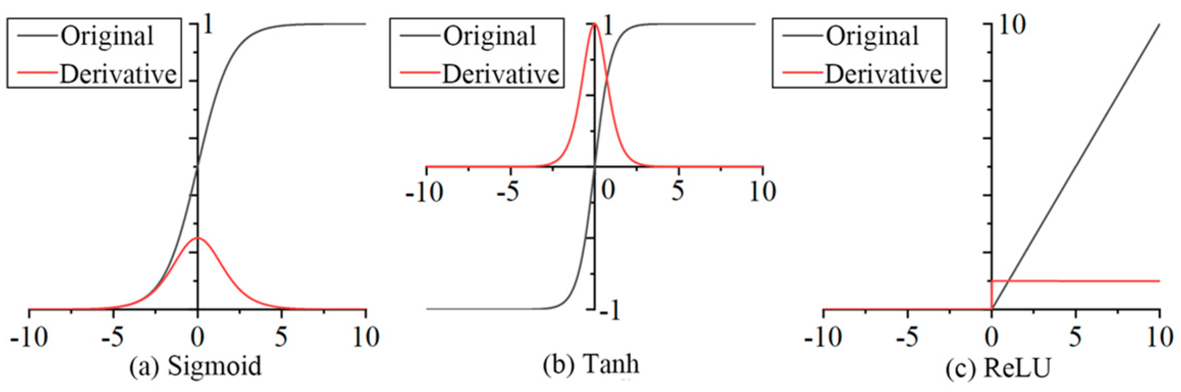
Because the network’s operation procedures, such as convolution and pooling, are linear, it cannot describe complex nonlinear situations. As a result, a nonlinear activation function must be added after each layer of network operation. The Sigmoid, Tanh, and ReLU functions are examples of common neural network activation functions. (2) shows their mathematical expression.
Figure 9 depicts images of the Sigmoid, Tanh, and ReLU functions. The ReLU function is straightforward to use, and the derivative is always one when the input is positive, so the gradient does not disappear. The ReLU function’s derivation procedure is relatively simple, which is useful for calculating network backpropagation. At the moment, the ReLU activation function is used by the majority of CNN models.
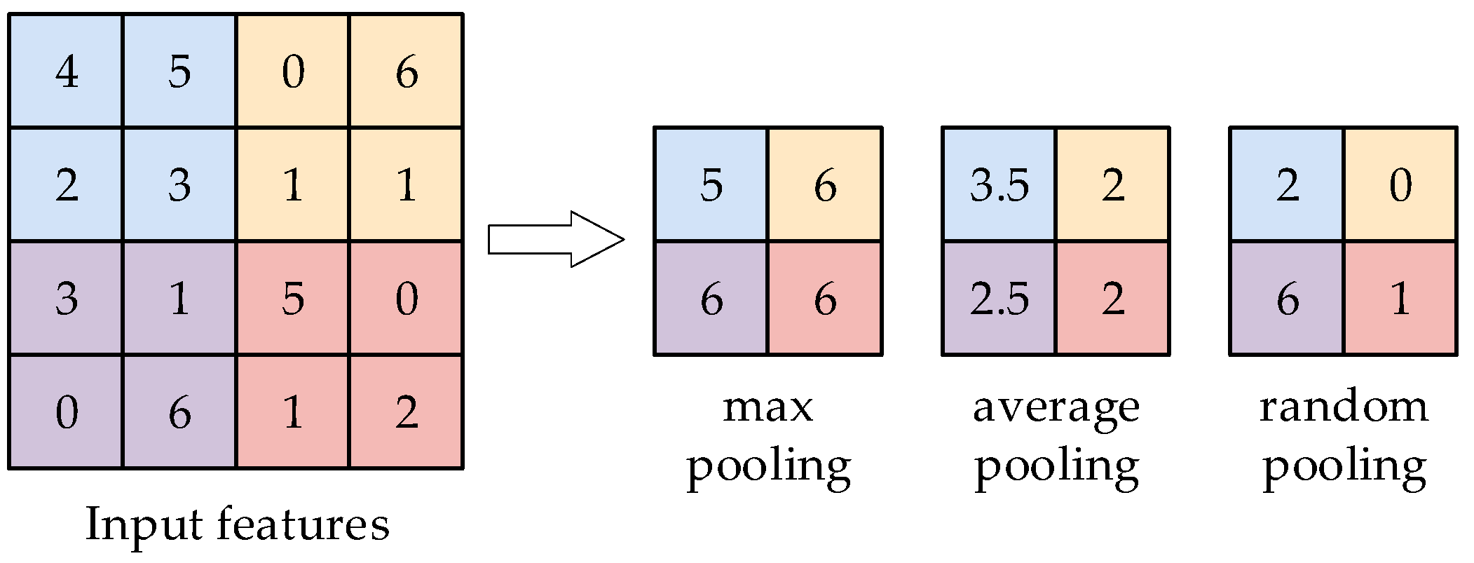
The pooling layer is responsible for down-sampling the feature map based on the given area. Pooling computation can be categorized into maximum pooling, average pooling, and random pooling, as shown in Figure 10. The pooling layer can decrease the redundant data in the network and enhance the operating speed. The pooling layer can withstand slight disturbances from the input layer, thus improving the neural network’s robustness.
To obtain CNN’s classification function, the fully connected layer translates the features collected by the convolutional layer to the sample label space. The Softmax function can normalize the fully linked layer’s output to the (0, 1) interval. The total of all output values is one, which is consistent with the probability distribution and yields the intuitive maximum probability as a classification result. Softmax makes it easier to calculate the derivative of the network loss function and train the network.
The higher the recognition accuracy, the stronger the network expression performance and the more complicated the convolutional neural network model. Complex models necessitate a substantial amount of storage space and computer power, which are challenging to implement on embedded devices [22]. The high-complexity network cannot match the arc detection’s real-time requirements. To achieve real-time arc fault detection, it is important to investigate the neural network lightweight method and create a lightweight arc fault detection model.
The lightweight network method entails lowering the amount of convolution layer calculation and developing a more efficient network layout. It primarily includes Artificial Design Lightweight Network Models (ADLNM) [23], Convolution Neural Network Model Compression (CNNMC) [24], and automatic design neural network based on neural Network Architecture Search (NAS) [25]. Table 2 shows the specific comparison of these methods. NAS cannot eliminate human interference and requires the artificial definition of the search space and search technique. CNNMC can effectively reduce the number of parameters, but its accuracy will be slightly reduced as a result. ADLNM, which has been extensively utilized on embedded platforms, is best suited for AC fault identification and can also efficiently reduce the number of parameters.
3.2. Effnet Neural Network
MobileNet [20], ShuffleNet [26], and EffNet [27] are examples of common artificially built lightweight models. The overarching goal is to optimize the convolution calculation process while reducing the amount of model parameters and calculations.
EffNet optimizes the calculation of the convolution layer based on MobileNet and ShuffleNet. Spatially Separable Convolution (SSC) is added to depthwise separable convolution (DSC), which reduces the number of convolution layer parameters and calculation and optimizes the sharp reduction of data flow in common lightweight neural networks such as MobileNet and ShuffleNet, resulting in a decreased accuracy.
The DSC contains both depthwise and pointwise convolutions. The dimension size of the convolution kernel feature map is shown in (3).
is the size of the output feature map, m is the size of the input layer, and k is the size of the convolution kernel.
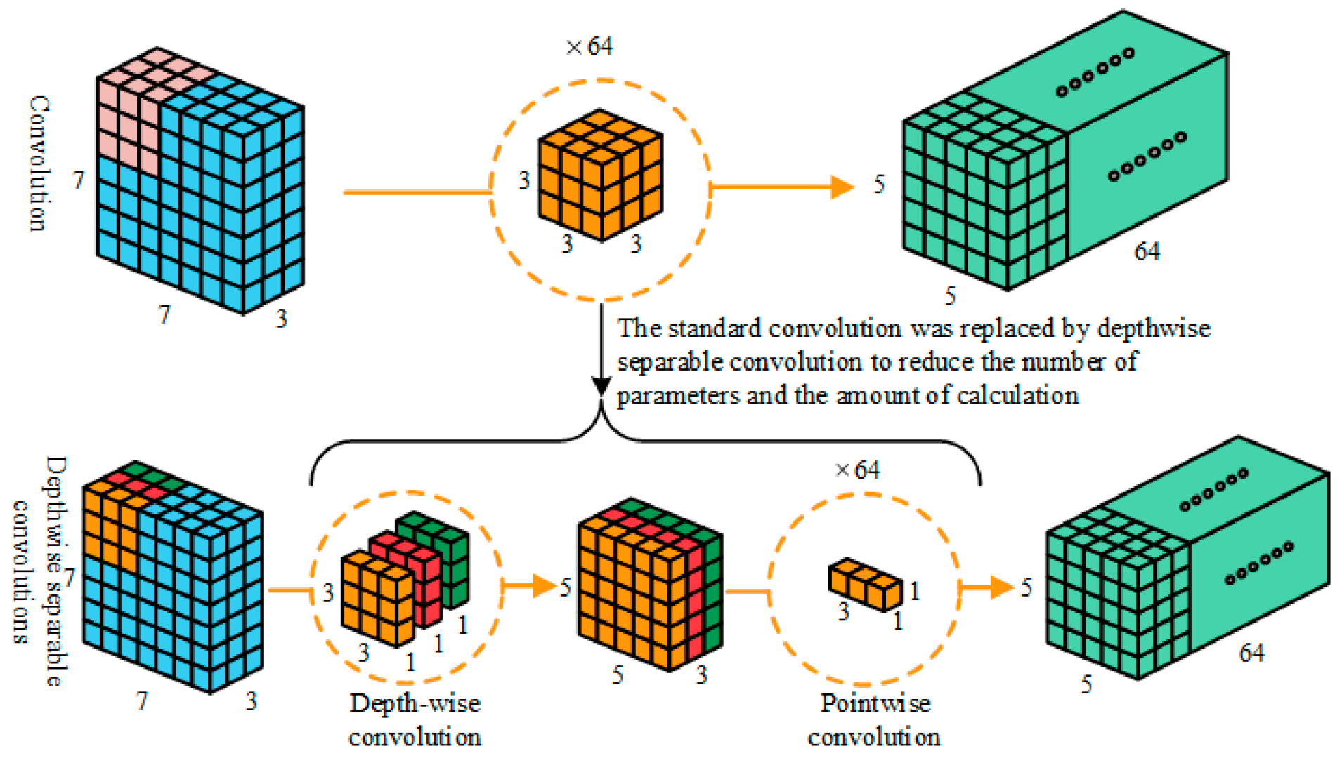
The standard convolution (SC) calculation procedure is depicted in the upper part of Figure 11. It is assumed that there are 64 convolution kernels. After the convolution operation, 64 feature maps with a size of 5 × 5 × 1 are obtained. The output of the convolution layer of 5 × 5 × 64 is obtained after merging. The spatial dimension of the data reduces and the depth increases after the convolution calculation.
The lower half of Figure 11 depicts the DSC calculation process. Firstly, the convolution is calculated by depth convolution, and the convolution kernel of 3 × 3 × 3 is replaced by three convolution kernels of 3 × 3 × 1. Each convolution kernel corresponds to a channel of the input layer, corresponding to the three colors of yellow, red, and green in Figure 11. Each convolution can obtain a 5 × 5 × 1 feature map, and the three channels obtain a feature map with a size of 5 × 5 × 3. Then, point-by-point convolution calculation is performed, and the convolution kernel size is 1 × 1 × 3. After this calculation, a feature map with a size of 5 × 5 × 1 is obtained. After 64 operations, the output feature map of the same size as the SC calculation is obtained. The parameter size and calculation amount of the standard convolution are shown in (4).
is the parameter amount, and is the calculation amount. W, H, and M are the length, width, and height of the neural network input layer, K is the size of the convolution kernel, and N is the number of convolution kernels. The amount of the DSC is shown in (5).
In (6), the DSC parameter and calculation amount are 1/N + 1/K2 times that of SC. Using N = 64, K = 3, the parameter and computation amount of the DSC are lowered by 87.3%, when N = 64, K = 3.
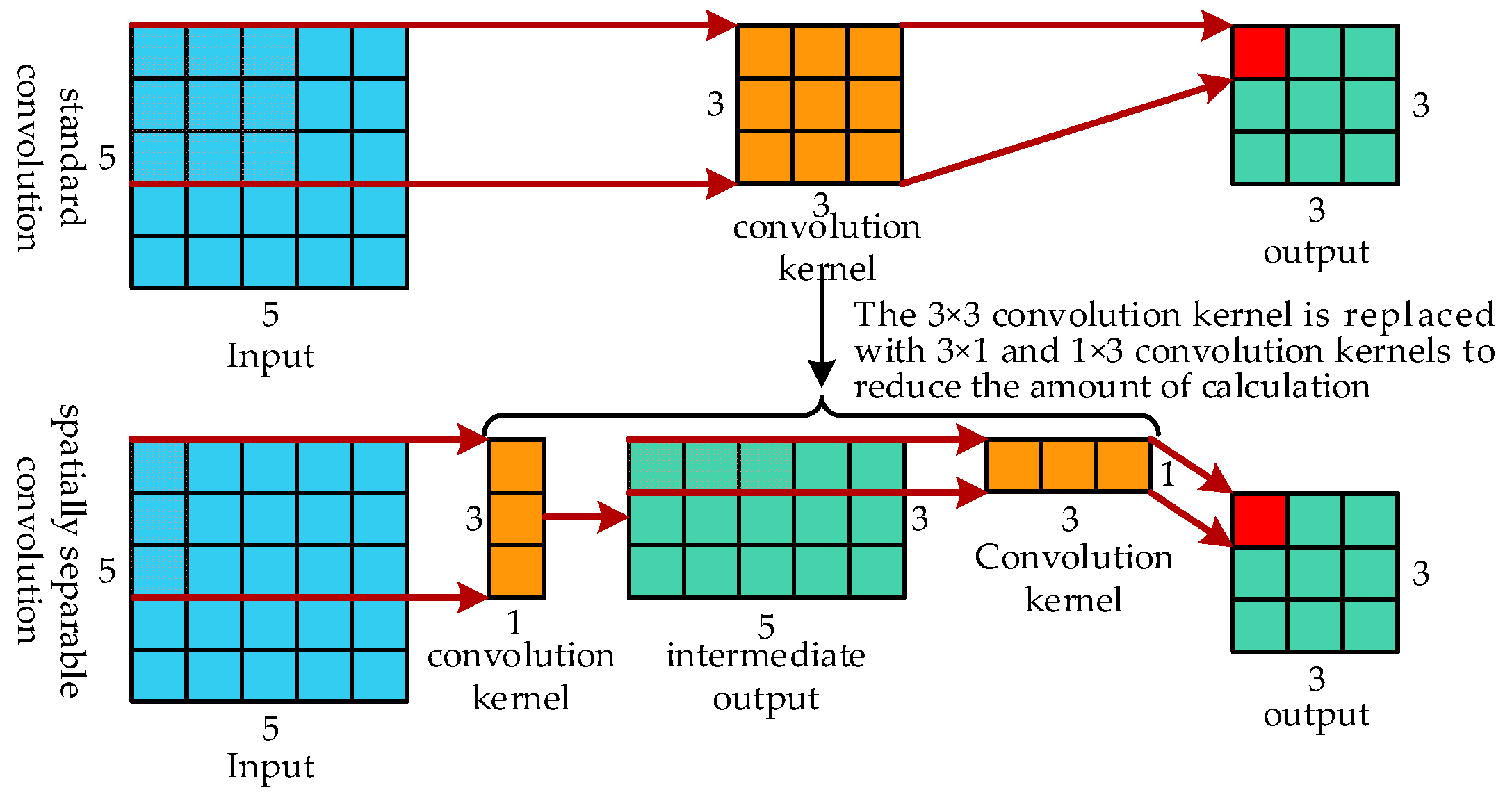
The fundamental idea behind SSC is to use the spatially aggregation process of low-dimensional convolution in place of the typical high-dimensional convolution. The data on the adjacent regions of the convolutional neural network feature map are highly correlated, and the spatially aggregation process of low-dimensional convolution will not result in a network expression ability loss [28]. A convolution kernel of 3 × 3 is divided into two convolution kernels of 3 × 1 and 1 × 3, as seen in Figure 12.
Convolution calculation is simplified using SSC. The size of the neural network’s input is W × W, and the size of the convolution kernel is K × K. (7) and (8) demonstrate the computation amount of SC and SSC operations.
By dividing (7) by (8), we obtain (9). When W = 5, K = 3, and (9) is 0.889. In other words, the amount of calculation is reduced by 11.1%.
The neural network data flow is the output data amount for each network layer in the model. The reduction in data flow will result in a certain data loss, lowering the accuracy of model recognition. Large networks’ width and depth can compensate for information loss caused by a reduction in data flow. The depth and width of the lightweight network model are limited, as is its accuracy rate [25]. EffNet takes on the data flow bottleneck problem of MobileNet and ShuffleNet by adjusting the number of channels in the network input layer. Table 3 shows the data flow of three typical models. The output data amounts for the different network layers are given by the numbers provided in Table 3. Using MobileNet as an example, the SC + P network layer’s output data amount of 16,384 is also the DSC network layer’s input data amount. Data information loss occurs from the DSC network layer’s 4096 output data amounts, and a change multiple of its input and output is higher than or equal to 4 [25]. The red-marked number indicates a data bottleneck at this network layer. Data bottlenecks exist on MobileNet and ShuffleNet, but not on EffNet. In Table 3, SC is standard convolution, P is pooling, DSC is depthwise separable convolution, SSC is spatially separable convolution, and FC is fully connected layer.
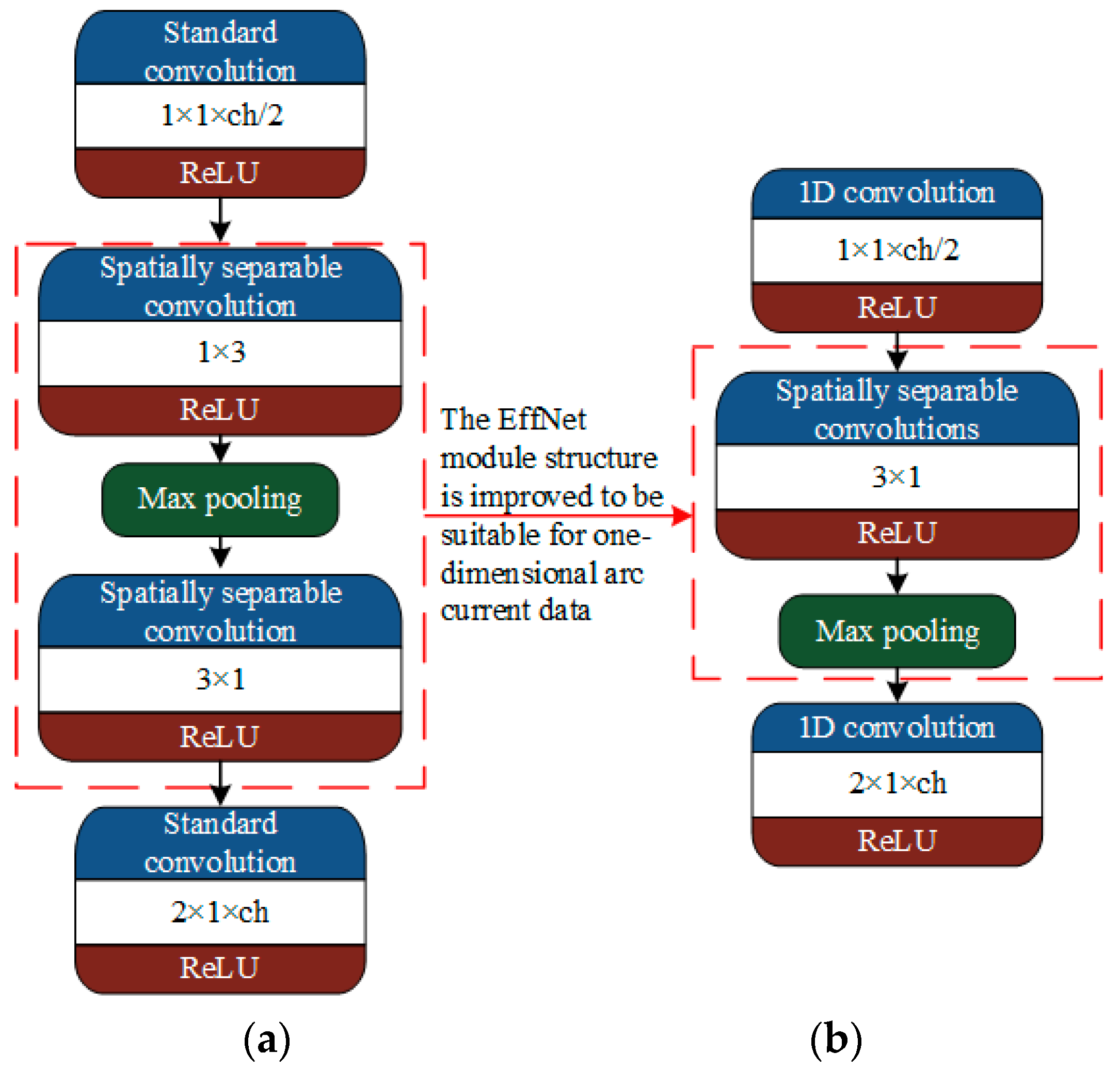
EffNet creates a general module that optimizes the convolution computation process in the classic network model. The structure is shown in Figure 13a. ch is the number of convolution kernel channels. The module’s input is a convolution layer of 1 × 1, and the number of channels (the number of convolution kernels) is half of that of MobileNet and ShuffleNet. The module’s middle two layers are convolution calculations, which are SSCs of 1 × 3 and 3 × 1. There is a maximum pooling layer after the first convolution computation to reduce the network parameters. The output layer of the module is 2 × 1 convolutional layer, the same as MobileNet and ShuffleNet.
4. Methodology: Arc_EffNet
4.1. Improved Effnet Model
The EffNet module contains a 1 × 3 size convolution kernel, which means that the input data length and width must be at least one and three. Therefore, the EffNet network model is suitable for two-dimensional data with widths over three. Because the current is a one-dimensional time series data, EffNet cannot be used to directly identify the series arc fault. As a consequence, the EffNet module is improved, and a lightweight arc fault detection model Arc_EffNet is proposed, which can be trained using one-dimensional current data. The EffNet module and Arc_EffNet module structures are shown in Figure 13.
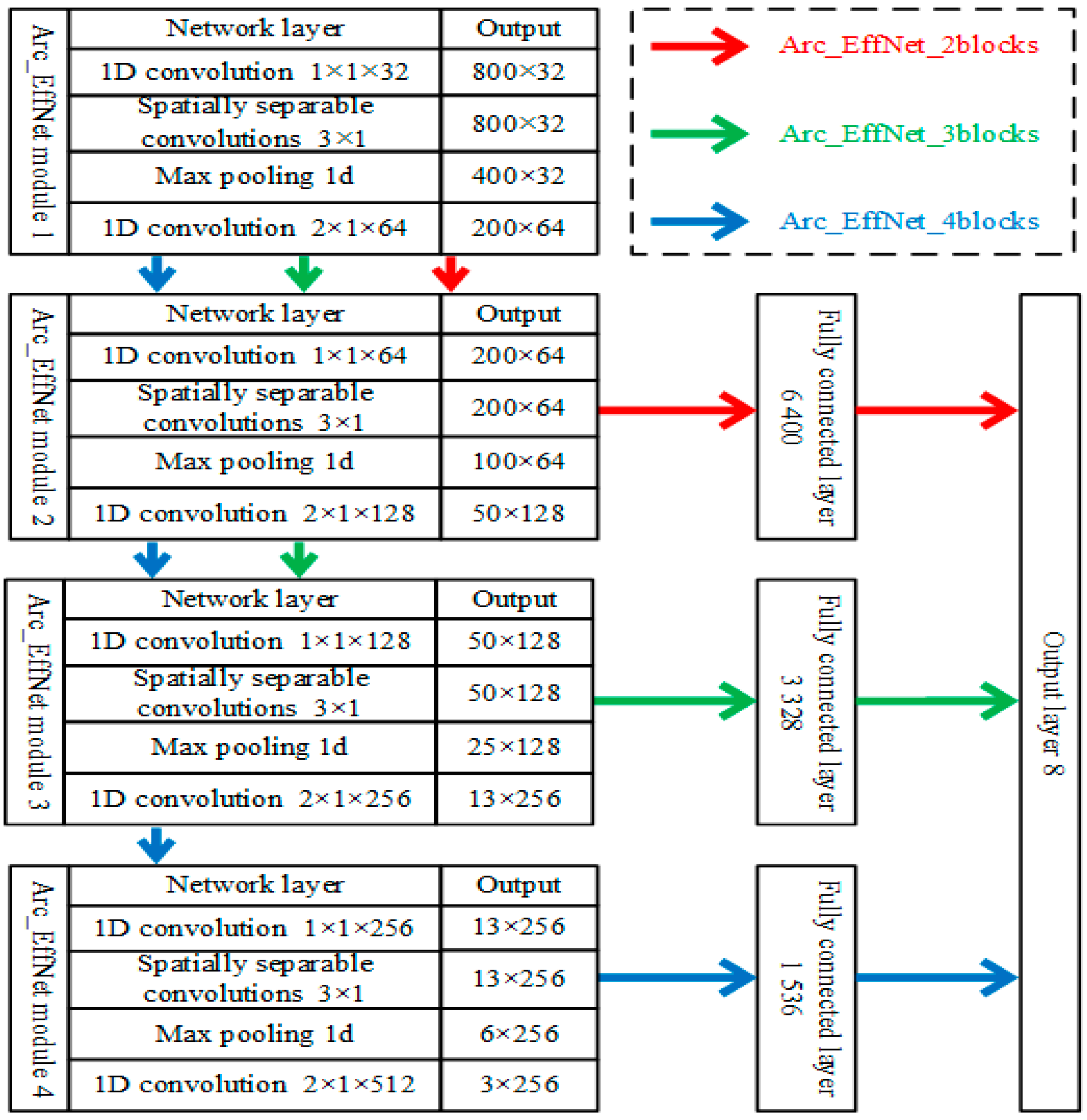
The Arc_EffNet module consists of three layers. A one-dimensional convolutional layer of 1 × 1 is used as the input layer. The middle layer is an SSC layer of 3 × 1 and a maximum pooling layer with a step size of 2. The last layer is a one-dimensional convolutional layer of 2 × 1, with a step size of 2. The Arc_EffNet module, which can be used for one-dimensional arc data, retains the SSC function of the classic EffNet module. To eliminate the data flow bottleneck, the number of convolution kernel channels in the final layer must be double that of the previous two layers. The Arc_EffNet module is built with Keras (the input data of the module is 800 × 1 arc fault current samples), and the specific structural parameters of the module are shown in Table 4.
The Arc_EffNet model consists of several Arc_EffNet modules. The appropriate number of modules and hyperparameters is necessary to achieve the model’s best results. The model depth has a direct impact on the number of parameters and recognition accuracy. The proper number of modules is chosen to assure the Arc_EffNet model’s accuracy while minimizing the number of model parameters and the amount of model calculations.
The classic EffNet network uses three modules. According to the EffNet model, the number of modules selected is 2, 3, and 4, which are recorded as Arc_EffNet_2blocks, Arc_EffNet_ 3blocks, and Arc_EffNet_4blocks. The structure of the three models is shown in Figure 14. When n is four, the output length of fourth module is reduced to three. If we continue to increase the module number, the input dimension of the fifth module is lower than the size of the convolution kernel, and a large number of ‘0’s needs to be added to the convolution, and too many ‘0’s will lead to a network training failure. The number of modules n should be less than or equal to four.
The arc dataset is created to optimize the model and evaluate its performance. The original current data is collected using the arc fault experimental platform. Data preprocess consists of four steps: data segmentation, normalization, cleaning, and labeling.
The size of the input data must adhere to rigorous guidelines, and each sample’s size within the dataset must be constant. A power frequency cycle (20 ms) is employed as the fundamental segmentation unit because the AC arc fault is periodic and may preserve the features of sample waveform symmetry. The length of a single sample is 800 since the data sampling rate is 40 kHz.
Small current data will be buried by large current data due to the wide range of the arc current, making it impossible to properly extract features. Thus, the incoming data are normalized. This paper uses [0, 1] normalization, as shown as (10). In the formula, and are the maximum and minimum values in one data sample.
Model accuracy will be reduced during collection by anomalous data, such as waveform distortion and void data value. To increase the data quality, the arc current data needs to be cleaned. A total of 34,224 arc fault current samples, including 16,026 arc samples and 18,198 non-arc samples, were collected after cleaning.
The data load type, arc state, and lack of arc are all marked. To obtain the arc fault current dataset, the arc data are marked with 0, 2, 4, and 6, the non-arc data are marked with 1, 3, 5, and 7, and the label is encoded with One-Hot. The model is trained using the training dataset, while the network hyperparameters are tweaked using the verification dataset to assess the level of network training. It is also required to establish a test dataset to gauge how well the network performs. The dataset is split into three portions based on 75%, 10%, and 15%, but the test set does not participate in the network training. The dataset details are displayed in Table 5.
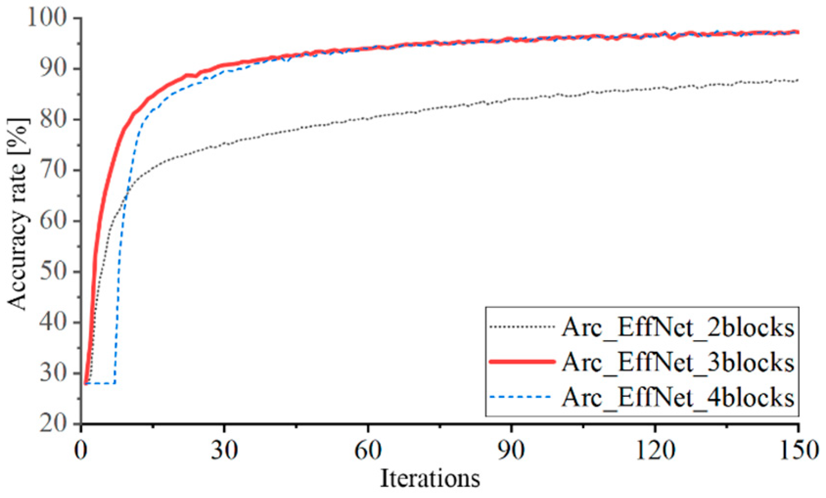
Figure 15 depicts the model training accuracy curve for various module counts. Only 87.88% of Arc_EffNet_2blocks are accurate. Arc_EffNet_3blocks has a 97.21% accuracy rate. The accuracy of the first seven epochs of Arc_EffNet_4blocks training remains unaffected as a result of the convolution complement ‘0’ and the pooling layer rejecting data, and the ultimate accuracy rate is 96.96%.
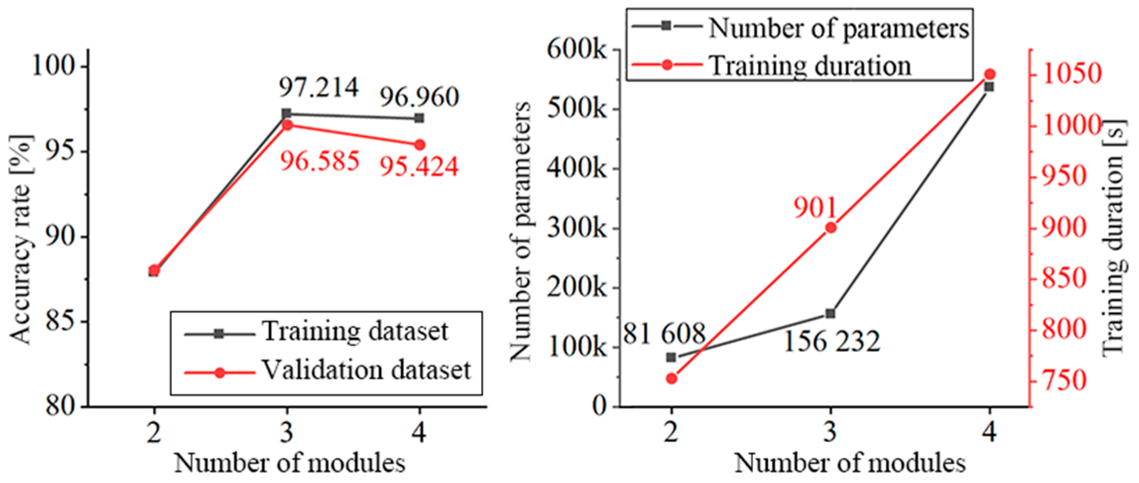
Figure 16 displays the training outcomes, the number of parameters, and the training duration for the three models. The least significant parameter for Arc_EffNet_2blocks was 81,608. Arc_EffNet_3blocks has a parameter that is 74,624 higher than Arc_EffNet_2blocks. Arc_EffNet_4blocks has the biggest parameter quantity, which is 3.4 times larger than Arc_EffNet_3blocks. Arc_EffNet_3blocks had the best accuracy, with 97.21% and 96.59%, respectively, in the training and validation sets. The time required for network training increases linearly as the number of modules increases. Finally, Arc_EffNet_3blocks with moderate parameters and the highest accuracy are selected as the arc fault recognition model.
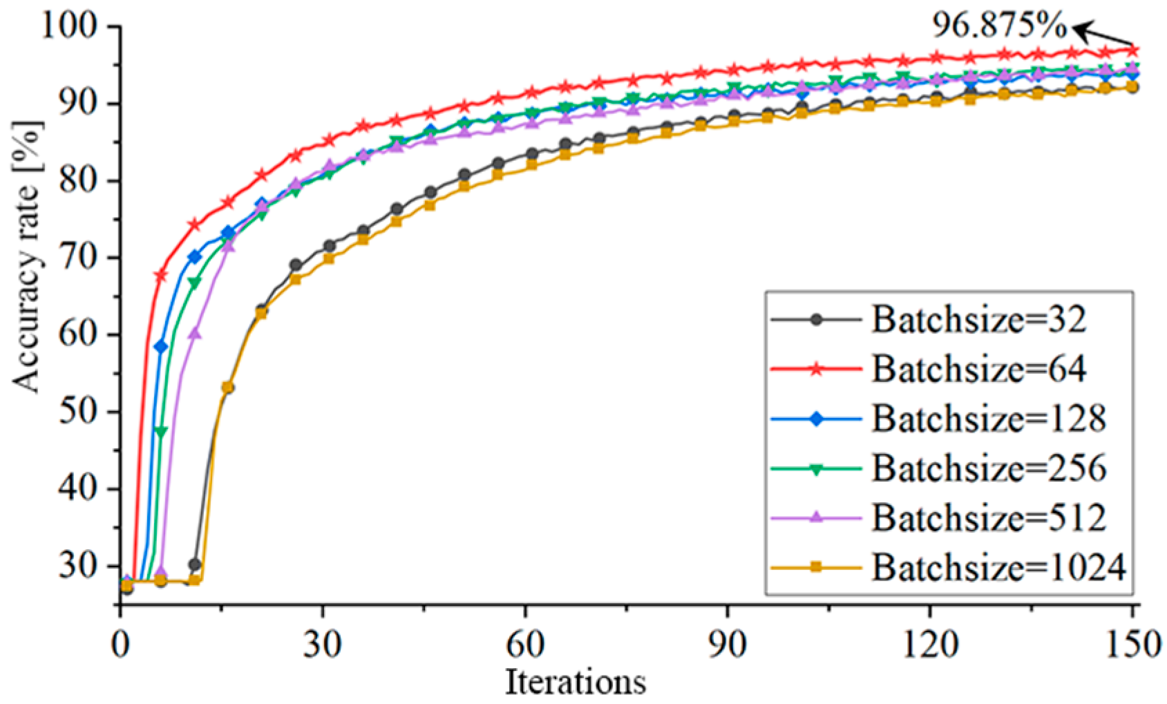
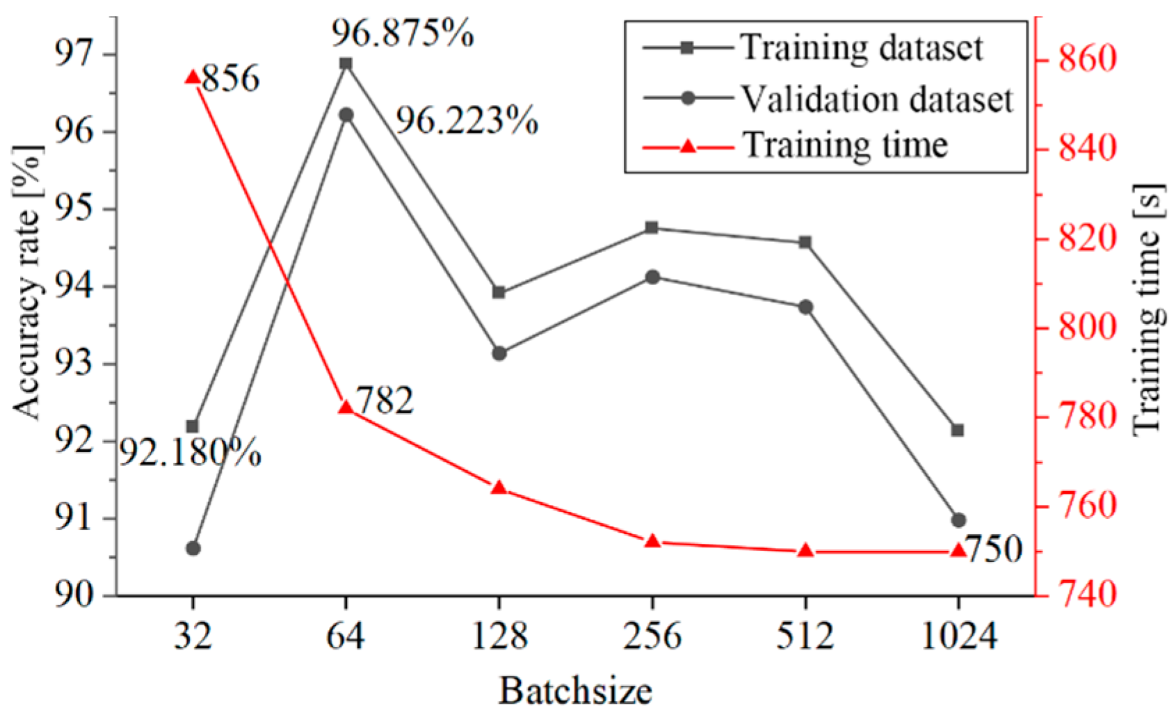
The quantity of data chosen for each neural network training is known as the Batchsize. Batchsize needs to be optimized because it influences training time and accuracy. Six different Batchsizes of 32, 64, 128, 256, 512, and 1024 were chosen for training, and Figure 17 displays the accuracy curve.
The ultimate accuracy and training time for various Batchsizes are shown in Figure 18. With an increase in Batchsize, the training time decreases, but the change in time is minimal, and the effect is negligible. Finally, 64 is chosen as the Batchsize.
4.2. Arc_EffNet Training Strategy Optimization and Result Analysis
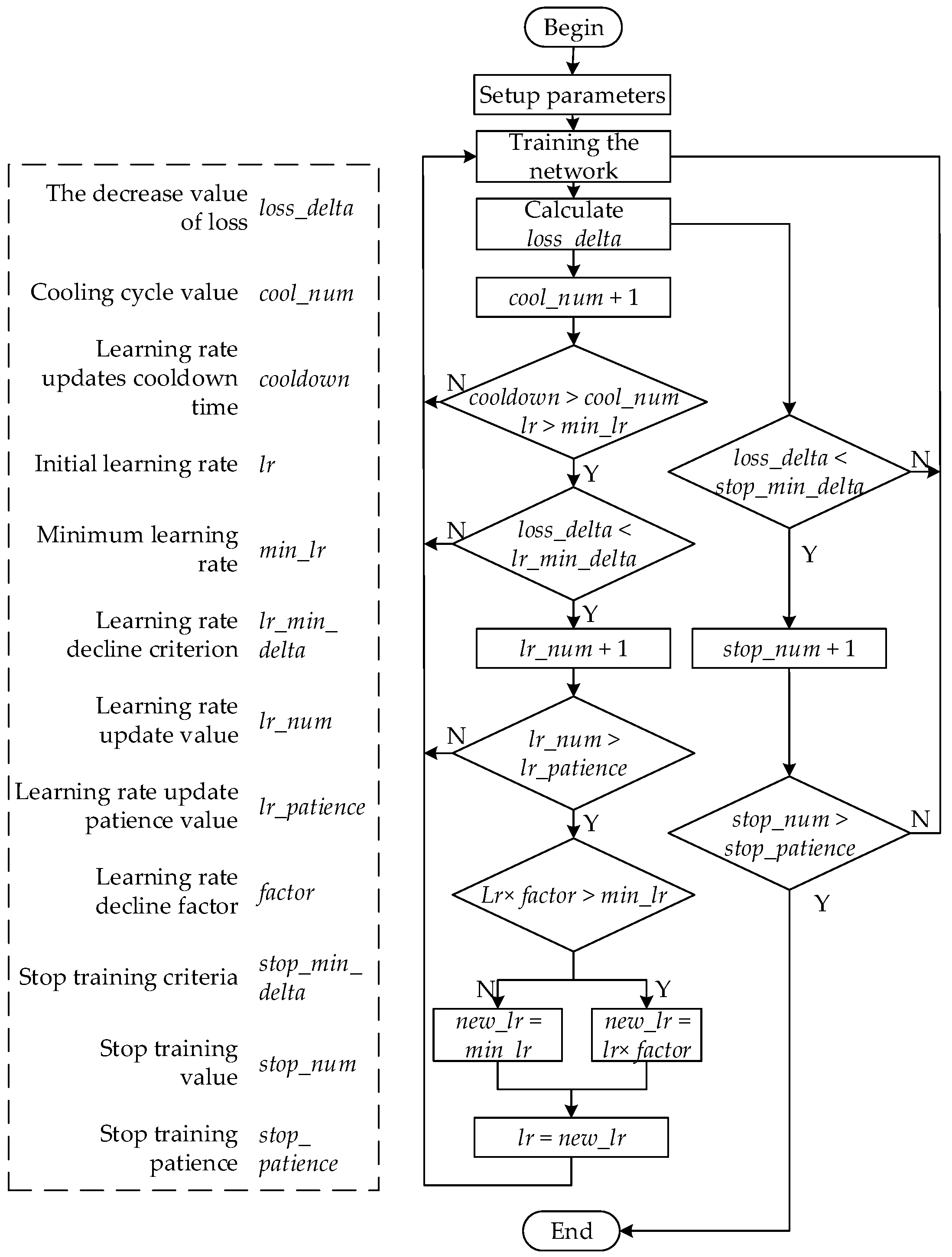
The learning rate of neural networks will have an impact on the network’s training duration and accuracy, and it may even cause the network to converge to the local optimal solution. As a result, it is suggested to use the network learning rate update strategy to change the learning rate in real time while Arc_EffNet is being trained. Early in the training process, a high learning rate is chosen in order to force the network to quickly converge and prevent it from settling for the local optimal solution. The network oscillation is decreased as a result of the training as it gradually lowers the learning rate, leading to the convergence of the best outcome. The network will not over-fit thanks to the addition of the automatic stop training strategy.
The learning rate update strategy and the automatic stop training strategy are shown in Figure 19. The two strategies use the loss value as the evaluation criterion. We set a learning rate update patience value (lr_patience) to avoid the learning rate from rapidly dropping to the minimal value due to the fluctuation loss value during training. If the loss value decreases continuously near 0 in the later stage of network training, the neural network training will fail; thus, the minimum learning rate (min_lr) is set. The learning rate is set and the cooling time is updated to avoid the network from falling into the local optimal solution due to the continuous updates of the learning rate.
In the process of training, the learning rate update strategy and the automatic stop training strategy are implemented simultaneously. After completing a training epoch, the decrease value of loss (loss_delta) is calculated, and it is compared with the minimum decrease value (stop_min_delta) that we had set. When loss_delta continues to be less than stop_min_delta and the number of cycles (stop_num) is greater than the patience value, we intend to stop training (stop_patience), and thus, training will stop. Through the above method, the training time can be reduced, and the network overfitting can be avoided.
The parameters of the learning rate update strategy and the automatic stop training strategy are based on the test results to select the optimal parameters. Table 6 shows all the hyperparameter values of the arc fault detection model.
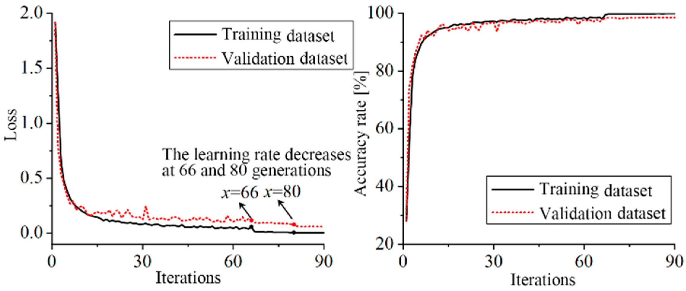
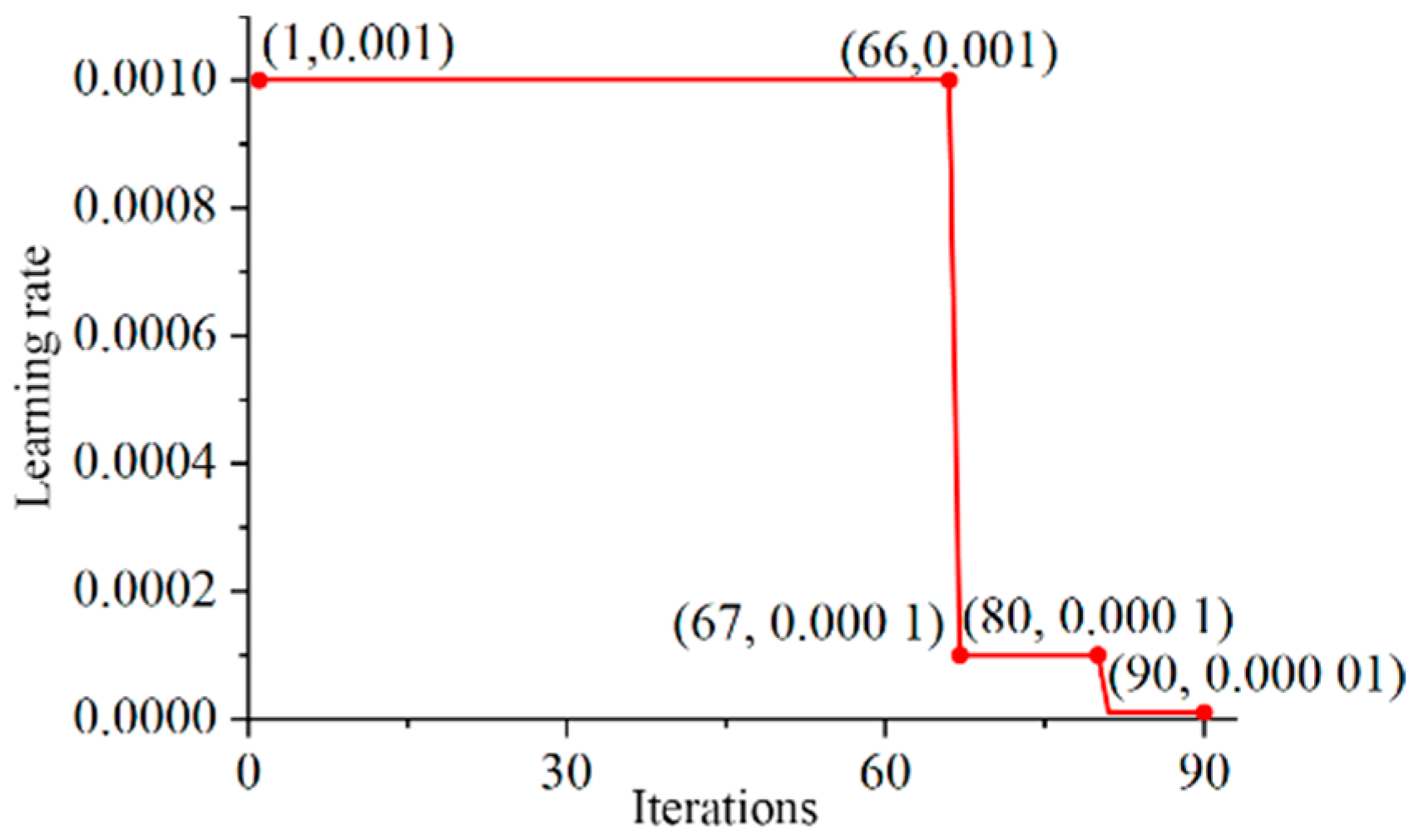
The model training curve is shown in Figure 20 and Figure 21. At the 66th epoch, the loss value of five consecutive cycles is less than the criterion, and the excessive learning rate leads to oscillation. At this time, the learning rate is reduced for the first time, the gradient descent step is reduced, the loss value of the training set network continues to decrease, and the accuracy is further improved. In the 80th epoch, the learning rate was reduced again, reaching the minimum learning rate of 0.00001. The loss value of continuous 10 epochs of training was not reduced, and the training was automatically stopped to prevent overfitting. Finally, the accuracy of the Arc_EffNet training dataset is 99.90%, and the accuracy of the verification dataset is 98.57%. There is no overfitting and underfitting in the training process, which proves the effectiveness of the network learning rate update strategy and the automatic stop strategy.
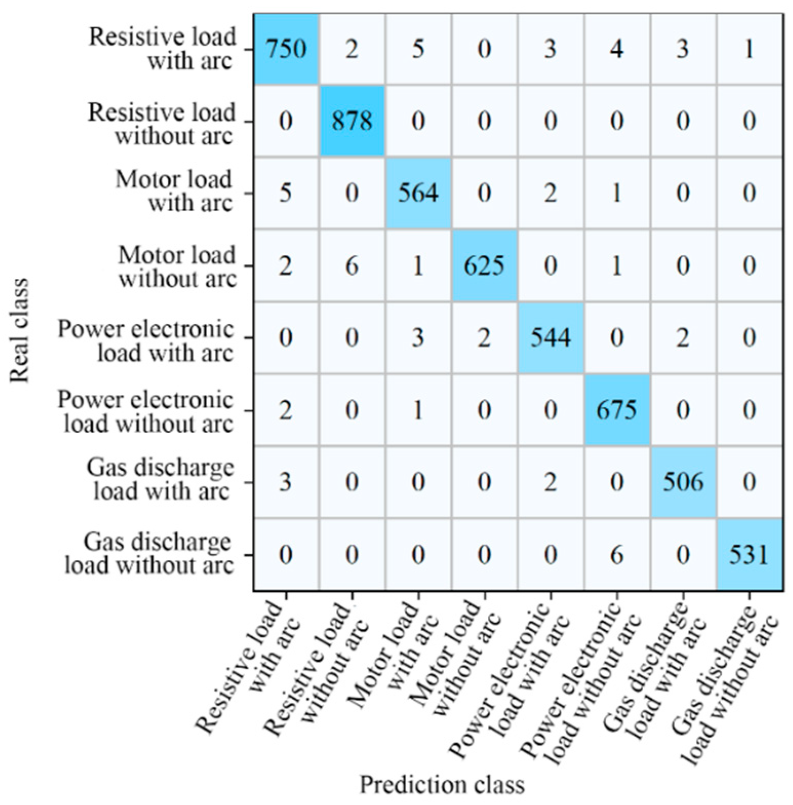
The test dataset verifies the performance of the Arc_EffNet model. The confusion matrix of model prediction results are shown in Figure 22. The horizontal axis of the matrix is the model prediction category, and the vertical axis is the actual category. Diagonal data are the number of correctly identified samples. The number of samples with prediction errors is 57, and 41 of these belong to load category detection errors. These errors have little effect on arc detection and are not misjudged or missed.
From the perspective of arc recognition, there are 16 samples with detection errors, and the detection errors are mainly concentrated on resistive load, motor load, and power electronic load. The arc current waveform of resistive and motor loads is similar to the normal current waveform of power electronics; thus, there are few detection errors.
The precision, recall, and accuracy of Arc_EffNet are shown in Table 7. The experimental results prove the effectiveness of the optimization model in arc fault detection.
5. Arc Fault Detection Device
We compared the commonly used embedded devices to verify the feasibility of the Arc_EffNet deployed in embedded devices. We selected Raspberry Pi 4B as the basis for building an AFDD. To deploy the model on a Raspberry Pi, Arc_EffNet is converted using TensorFlow Lite. The algorithm is designed to achieve the detection of arc faults. Finally, the AFDD is tested and verified.
5.1. Arc Fault Detection Device Design
The embedded device is used to obtain signal processing functions, and the Arc_EffNet network model is run to detect the arc fault and control the tripping circuit. To select the appropriate embedded platform, the common embedded platforms used in artificial intelligence, including MAIX Dock, Raspberry Pi 4B, and FPGA, are compared, as shown in Table 8.
MAIX Dock is an AIOT development board designed based on the edge intelligent computing chip K210. MAIX Dock has a neural network processor (KPU) that can perform hardware acceleration of convolution, pooling, and activation operations, but its acceleration can only be targeted at specific convolution calculations, and model deployment is complex.
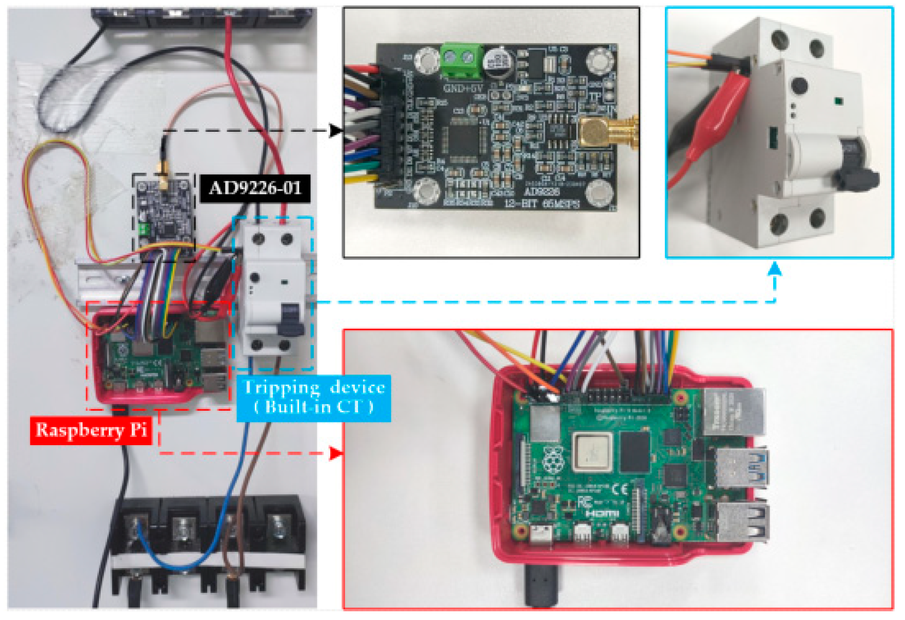
Raspberry Pi 4B is a microcomputer based on a Linux system, widely used in artificial intelligence fields such as face recognition and intelligent speakers. The CPU of Raspberry Pi 4B is ARM Cortex-A72, with a maximum frequency of 1.5 GHz and a maximum memory of 4 GB. Its performance is sufficient to support the regular operation of the arc fault detection model. The Raspberry Pi model is more convenient to deploy, and the TensorFlow Lite can be directly used to deploy the arc fault detection model. Compared with MAIX Dock, Raspberry Pi 4B is more expensive. Importantly, the Raspberry Pi is used for hardware-in-loop based fast verification of the proposed algorithm due to the core of Raspberry Pi being similar to that used in existing AFDD, such as STM32 series MCUs. Therefore, this paper uses Raspberry Pi 4B to build an AFDD. The AD module uses AD9226-01, and the maximum sampling rate can reach 65 MHz. This paper sets it to 40 kHz.
TensorFlow Lite is an open-source deep learning framework that helps developers run TensorFlow models on embedded devices with limited storage and computing resources. The TensorFlow Lite is used to convert the Arc_EffNet model, the TensorFlow interpreter is installed on the Raspberry Pi to run the model, and the arc fault recognition algorithm is designed. The calculation time of the device was tested, as shown in Table 9. Sample amount represents the number of samples processed in one test. The average time for the Raspberry Pi 4B to run the Arc_EffNet model and to predict a sample was only 0.2 ms.
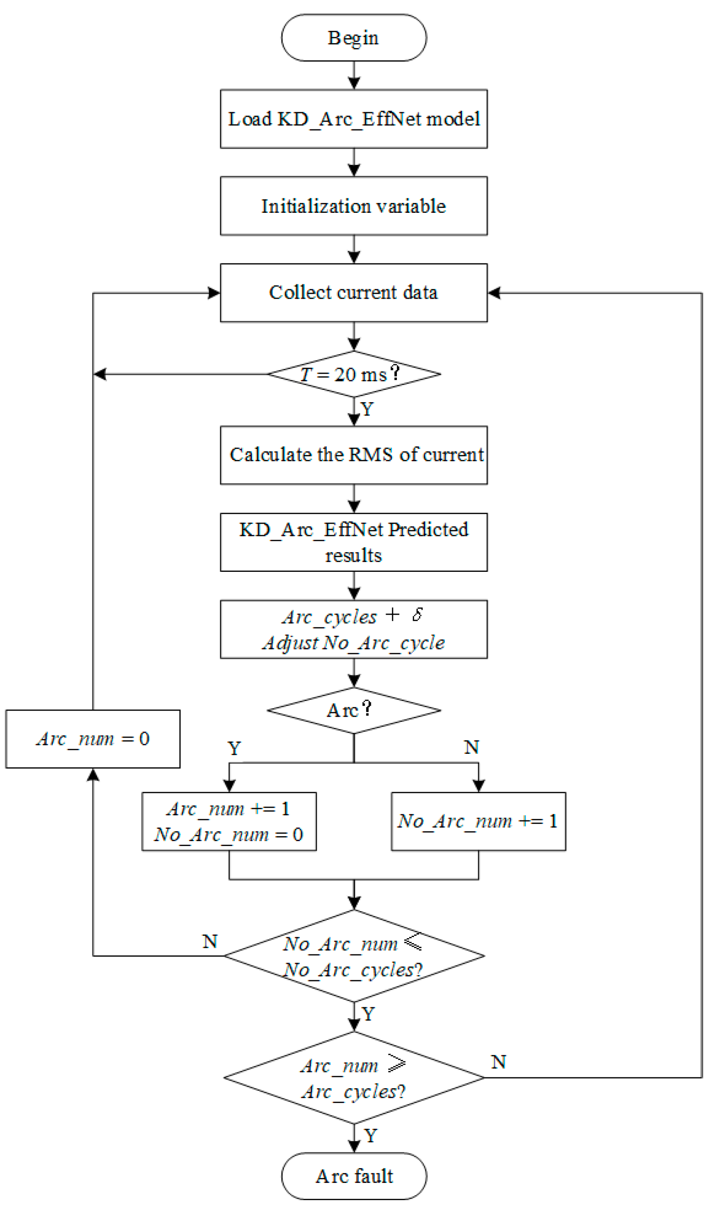
The IEC 62606 standard stipulates that the tripping time of AFDD is different at different current levels; thus, the number of arc fault cycles Arc_cycles is set in the design of the arc fault detection algorithm to control the tripping time. In addition, according to the load class predicted by the model, Arc_cycles are fine-tuned again (+δ) to improve the reliability of the inspection device. The algorithm chart is shown in Figure 23.
The Arc_EffNet model is loaded after the detection device is powered on. The initial arc accumulation value Arc_num is 0, non-arc accumulation value No_Arc_num is 5, the number of arc fault detection cycles Arc_cycles is 25, and δ is 0. Arc_cycles is adjusted according to the calculated current value. The normalized current data is inputted into the Arc_EffNet model. After an experimental verification, the final algorithm parameter values are shown in Table 10.
5.2. Experimental Verification
The arc fault detection device is shown in Figure 24. The AD module transmits data to Raspberry Pi 4B through SPI communication. Raspberry Pi runs the software algorithm to identify the arc fault. When the arc fault is detected, the circuit is cut off. Part of the load used in the experiment is shown in Figure 25.
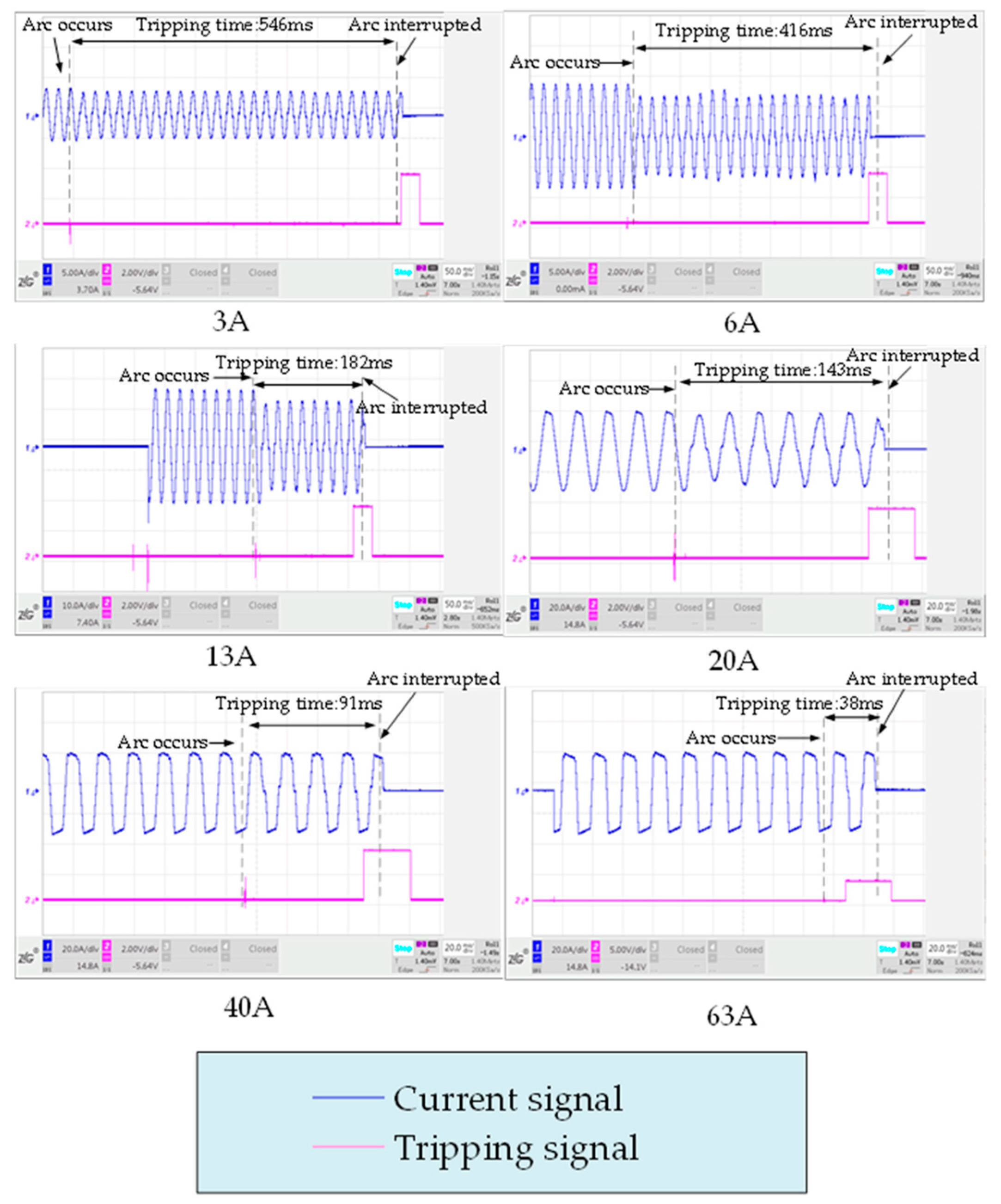
The test results of the series arc fault are shown in Table 11. For every current level, the arc experiments are repeated three times for complying with the standard requirements. The trip time of the AFDD under each current level meets the requirements of IEC 62606. The high current level arc fault is very harmful, and the shorter trip time is beneficial to suppress the arc risk. The low current arc fault level is less harmful, and the longer trip time can avoid miss-operation and rejection. Figure 26 depicts the waveform of the series arc tests. Figure 26 shows the locations of the arc’s occurrence and interruption, as well as the tripping time.
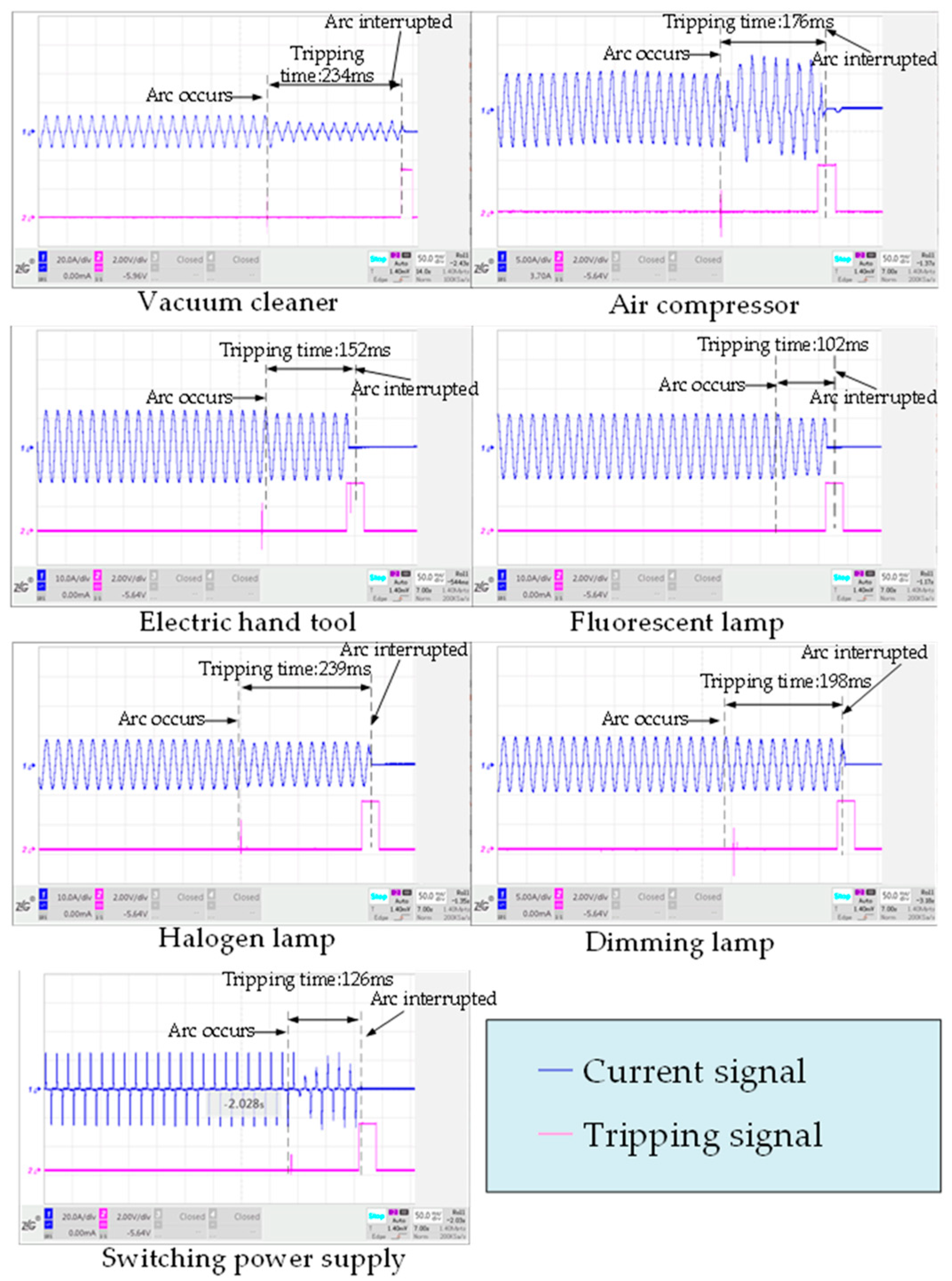
The seven loads listed in Table 12 are masking loads specified in the IEC62606 standard. The masking test results are shown in Table 12. We have tested all four of the configurations, i.e., A, B, C, and D, that are required to be included in the shielding experiment according to the standards. The trip time of masking test also meets the requirements. The trip time is similar because each load is at the same current level. Figure 27 depicts the waveform of the masking tests.
6. Conclusions
This paper proposes a lightweight detection method for series arc faults based on improved EffNet, a type of convolutional neural network. Based on the analysis of arc features in the time domain, the raw arc current data is selected as the input of the proposed algorithm, which can help reduce the complexity of the EffNet structure. Moreover, the first and last convolution layers of the EffNet module are improved by replacing standard convolution with one-dimensional convolution. Meanwhile, the spatially separable convolution is well-tuned and trimmed to achieve a more lightweight and better-performance architecture for arc fault detection called Arc_EffNet. The Arc_EffNet_3blocks architecture and the 64 Batchsize are used for the proposed algorithm, while an accuracy of 99.75% is achieved for the Arc_EffNet. In addition, a learning rate update strategy and an automatic stop training strategy during the training process are applied to accelerate the network training speed and prevent the network from settling for the local optimal solution and overfitting. Finally, a prototype based on the Raspberry Pi 4B is designed. As Raspberry Pi 4B has a similar micro-controller architecture to that used in commercial AFDDs, it can provide the suitable hardware for loop verification. Experimental results show that the run-time for processing a data sample of each power cycle of 20 ms is only about 0.2 milliseconds due to the high efficiency of the proposed Arc_EffNet model. It takes about 72 ms for the algorithm to take the final decision using multi-cycle detection that guarantees a robust confirmation. It is verified that the proposed method can fulfill the requirement of real-time detection for arc faults.
With the development of society, the field of electricity is becoming increasingly complex, and its associated security risks are also increasing. Therefore, in the subsequent study, it is necessary to evaluate the fire law of arc fault to reduce the risk of an arc fault.
Author Contributions
Conceptualization, X.N. and D.S.; methodology, X.N., D.S., and Y.W.; software, D.S., Y.W., and J.Z.; validation, D.S., J.Z., and Y.L.; formal analysis, X.N., Y.W., and H.Z.; investigation, Y.L.; resources, Y.W.; data curation, D.S. and X.L.; writing—original draft preparation, X.N., D.S., J.Z., and Y.L.; writing—review and editing, X.N., D.S., and Y.W.; visualization, H.Z. and X.L.; supervision, D.S. and Y.W.; project administration, X.N. and H.Z.; funding acquisition, X.N. All authors have read and agreed to the published version of the manuscript.
Funding
This work was supported by the Science and Technology Project of State Grid Co., Ltd. (project name: Research and Application of Key Technologies for Fire Protection and Fire Disposal of low-voltage power distribution Grid; Project No.: 5400-202326208A-1-1-ZN).
Data Availability Statement
The data presented in this study are available in this article.
Conflicts of Interest
The authors declare no conflict of interest.
References
- IEA. Electricity Market Report—Update 2023, IEA, Paris. 2023. Available online: https://www.iea.org/reports/electricity-market-report-update-2023 (accessed on 1 January 2023).
- Fire and Rescue Department. National Fire and Police Situation. 2022. Available online: https://www.119.gov.cn/article/41kpo4CAQyv (accessed on 1 March 2022).
- Campbell, R. Home Fires Caused by Electrical Failure or Malfunction, National Fire Protection Association. 2022. Available online: https://www.nfpa.org/-/media/Files/News-and-Research/Fire-statistics-and-reports/US-Fire-Problem/Fire-causes/osHomeElectricalFires.pdf (accessed on 20 March 2022).
- IEC 62606-2017; General Requirements for Arc Fault Detection Devices. 2017. Available online: https://webstore.iec.ch/publication/27190 (accessed on 20 March 2022).
- Yong, J.; Xiao, B. Accurate harmonic model of typical single-phase nonlinear load and its harmonic attenuation features. Proc. CSEE 2014, 19, 55–62. [Google Scholar]
- Zhu, G.; Mou, L. Optimal control of distributed harmonic governance of multi-feeder low-voltage distribution network. Trans. China Electrotech. Soc. 2016, 31, 25–33. [Google Scholar]
- Chen, S.; Li, X.; Xie, Z.; Meng, Y. Time–Frequency Distribution Feature and Model Simulation of Photovoltaic Series Arc Fault With Power Electronic Equipment. IEEE J. Photovolt. 2019, 9, 1128–1137. [Google Scholar] [CrossRef]
- Kim, J.C.; Neacşu, D.O.; Lehman, B.; Ball, R. Series AC Arc Fault Detection Using Only Voltage Waveforms. In Proceedings of the 2019 IEEE Applied Power Electronics Conference and Exposition (APEC), Anaheim, CA, USA, 17–21 March 2019; pp. 2385–2389. [Google Scholar]
- Ilman, A.F. Low Voltage Series Arc Fault Detecting with Discrete Wavelet Transform. In Proceedings of the 2018 International Conference on Applied Engineering (ICAE), Batam, Indonesia, 3–4 October 2018; pp. 1–5. [Google Scholar]
- Xu, N.; Yang, Y.; Jin, Y.; He, J. Identification of Series Fault Arc of Low-voltage Power Cables in Substation Based on Wavelet Transform. In Proceedings of the 2020 IEEE 5th International Conference on Integrated Circuits and Microsystems (ICICM), Nanjing, China, 23–25 October 2020; pp. 188–192. [Google Scholar]
- Wang, W.; Li, J.; Lu, S. Application of Signal Denoising Technology Based on Improved Spectral Subtraction in Arc Fault Detection. Electronics 2023, 12, 3147. [Google Scholar] [CrossRef]
- Moon, W.-S.; Kim, J.-C.; Jo, A.; Bang, S.-B.; Koh, W.-S. Ignition Features of Residential Series Arc Faults in 220-V HIV Wires. IEEE Trans. Ind. Appl. 2015, 51, 2054–2059. [Google Scholar] [CrossRef]
- Qiongfang, Y.; Gaolu, H.; Yi, Y. Low Voltage Ac Series Arc Fault Detection Method Based on Parallel Deep Convolutional Neural Network. In IOP Conference Series: Materials Science and Engineering; IOP Publishing: Bristol, UK, 2019; Volume 490, p. 7. [Google Scholar]
- Han, X.; Li, D.; Huang, L.; Huang, H.; Yang, J.; Zhang, Y.; Wu, X.; Lu, Q. Series Arc Fault Detection Method Based on Category Recognition and Artificial Neural Network. Electronics 2020, 9, 1367. [Google Scholar] [CrossRef]
- Yin, Z.; Wang, L.; Zhang, Y.; Gao, Y. A Novel Arc Fault Detection Method Integrated Random Forest, Improved Multi-scale Permutation Entropy and Wavelet Packet Transform. Electronics 2019, 8, 396. [Google Scholar] [CrossRef]
- Wang, Y.; Hou, L.; Paul, K.C.; Ban, Y.; Chen, C.; Zhao, T. ArcNet: Series AC Arc Fault Detection Based on Raw Current and Convolutional Neural Network. IEEE Trans. Ind. Inf. 2022, 18, 77–86. [Google Scholar] [CrossRef]
- Yang, K.; Chu, R.; Zhang, R.; Xiao, J.; Tu, R. A novel methodology for series arc fault detection by temporal domain visualization and convolutional neural network. Sensors 2020, 20, 162. [Google Scholar] [CrossRef] [PubMed]
- Wang, Y.; Zhang, F.; Zhang, S. A New Methodology for Identifying Arc Fault by Sparse Representation and Neural Network. IEEE Trans. Instrum. Meas. 2018, 67, 2526–2537. [Google Scholar] [CrossRef]
- Shen, Y.-L.; Xu, Z. Fast Detection of Weak Arc Faults Based on Progressive Singular-Value-Decomposition and Empirical Analyses. IEEE Access 2022, 10, 130586–130601. [Google Scholar] [CrossRef]
- Siegel, J.E.; Pratt, S.; Sun, Y.; Sarma, S.E. Real-time deep neural networks for internet-enabled arc-fault detection. Eng. Appl. Artif. Intell. 2018, 74, 35–42. [Google Scholar] [CrossRef]
- Liu, Y.; Guo, F.; Wang, Z.; Chen, C.; Li, Y. Study on spectral features of series arc fault based on information entropy. Trans. China Electrotech. Soc. 2015, 30, 488–495. [Google Scholar]
- Zeng, J.; Chen, Y.; Lin, X.; Qin, C.; Wang, Y.; Zhu, J.; Tian, L.; Zhai, Y.; Gan, J. An Ultra-lightweight Finger Vulture Real-time Segmentation Network. Acta Photonica Sin. 2022, 51, 287–302. [Google Scholar]
- Ido, F.; Lutz, R.; Anton, K. EffNet: An Efficient Structure for Convolutional Neural Networks. arXiv 2018, arXiv:1801.06434. [Google Scholar]
- Chang, L.; Hongtao, L. A Highly Efficient Training-Aware Convolutional Neural Network Compression Paradigm. In Proceedings of the 2020 IEEE International Conference on Multimedia & Expo Workshops (ICMEW), London, UK, 6–10 July 2020; pp. 1–6. [Google Scholar]
- Ge, D.; Li, H.; Zhang, L.; Liu, R.; Shen, P.; Miao, Q. Survey of Lightweight Neural Network. J. Softw. 2020, 31, 2627–2653. [Google Scholar]
- Zhang, X.; Zhou, X.; Lin, M.; Sun, J. ShuffleNet: An Extremely Efficient Convolutional Neural Network for Mobile Devices. In Proceedings of the 2018 IEEE/CVF Conference on Computer Vision and Pattern Recognition, Salt Lake City, UT, USA, 18–22 June 2018; pp. 6848–6856. [Google Scholar]
- Freeman, I.; Roese-Koerner, L.; Kummert, A. Effnet: An Efficient Structure for Convolutional Neural Networks. In Proceedings of the 2018 25th IEEE International Conference on Image Processing (ICIP), Athens, Greece, 7–10 October 2018; pp. 6–10. [Google Scholar]
- Szegedy, C.; Vanhoucke, V.; Ioffe, S.; Shlens, J.; Wojna, Z. Rethinking the Inception Architecture for Computer Vision. In Proceedings of the 2016 IEEE Conference on Computer Vision and Pattern Recognition (CVPR), Las Vegas, NV, USA, 27–30 June 2016; pp. 2818–2826. [Google Scholar]
Figure 1.
Arc fault experimental platform.

Figure 2.
Time domain waveform and spectrogram of resistance current. (a) Time domain waveform; and (b) Fourier transform spectrogram.
Figure 2.
Time domain waveform and spectrogram of resistance current. (a) Time domain waveform; and (b) Fourier transform spectrogram.

Figure 3.
Time domain waveform and spectrogram of vacuum cleaner current. (a) Time domain waveform; and (b) Fourier transform spectrogram.
Figure 3.
Time domain waveform and spectrogram of vacuum cleaner current. (a) Time domain waveform; and (b) Fourier transform spectrogram.

Figure 4.
Time domain waveform and spectrogram of vacuum cleaner starting current. (a) Time domain waveform; and (b) Fourier transform spectrogram.
Figure 4.
Time domain waveform and spectrogram of vacuum cleaner starting current. (a) Time domain waveform; and (b) Fourier transform spectrogram.

Figure 5.
Time domain waveform and spectrogram of fluorescent lamp current. (a) Time domain waveform; and (b) Fourier transform spectrogram.
Figure 5.
Time domain waveform and spectrogram of fluorescent lamp current. (a) Time domain waveform; and (b) Fourier transform spectrogram.

Figure 6.
Time domain waveform and spectrogram of switching power supply current. (a) Time domain waveform; and (b) Fourier transform spectrogram.
Figure 6.
Time domain waveform and spectrogram of switching power supply current. (a) Time domain waveform; and (b) Fourier transform spectrogram.

Figure 7.
Comparison of different load currents.

Figure 8.
Classical CNN structure diagram.

Figure 9.
Activation function images.

Figure 10.
Pooling calculation.

Figure 11.
Depthwise separable convolution calculation process.

Figure 12.
Spatially separable convolution calculation process.

Figure 13.
EffNet module structure and Arc_EffNet module structure. (a) EffNet module; and (b) Arc_EffNet module.
Figure 13.
EffNet module structure and Arc_EffNet module structure. (a) EffNet module; and (b) Arc_EffNet module.

Figure 14.
Arc_EffNet network with different number of modules.

Figure 15.
Training accuracy curve of the three models.

Figure 16.
Model accuracy, number of parameters, and training time with different numbers of Arc_EffNet modules.
Figure 16.
Model accuracy, number of parameters, and training time with different numbers of Arc_EffNet modules.

Figure 17.
The training accuracy for different Batchsizes.

Figure 18.
Accuracy and training time for different Batchsizes.

Figure 19.
Learning rate update strategy and automatic stop training strategy.

Figure 20.
Loss value and accuracy of Arc_EffNet.

Figure 21.
Learning rate of Arc_EffNet.

Figure 22.
Confusion matrix.

Figure 23.
Arc fault detection algorithm.

Figure 24.
Arc fault detection device.

Figure 25.
Test load.

Figure 26.
Results of series arc tests.

Figure 27.
Results of masking tests.


Table 1.
Testing loads.
| Load Type | Load | Power | |
|---|---|---|---|
| Linear load | Resistive load | Resistor | - |
| Nonlinear load | Motor load | Vacuum cleaner | 1200 w |
| Air compressor | 2200 w | ||
| Electric hand tool | 650 w | ||
| Gas discharge lamp load | Fluorescent lamp | 900 w | |
| Dimming lamp | 1000 w | ||
| Power electronics load | Switching power supply | 700 w | |
| Halogen lamp | 1500 w | ||
Table 2.
Neural network lightweight method.
| Method | Feature | Suitable for Arc Detection or Not |
|---|---|---|
| ADLNM [23] | more efficient convolution calculation | yes |
| CNNMC [24] | small decrease in accuracy and significant reduction in parameters | no |
| NAS [25] | long time for network design and cannot get rid of human influence | no |
Table 3.
Different neural network data streams.
| MobileNet [20] | ShuffleNet [26] | EffNet [27] | |||
|---|---|---|---|---|---|
| Network Layer | Data Amount | Network Layer | Data Amount | Network Layer | Data Amount |
| SC + P | 16,384 | SC + P | 16,384 | SC SSC + P SSC SC | 32,768 16,384 16,384 16,384 |
| DSC SC | 4096 8192 | GC DSC GC | 8192 2048 8192 | SC SSC + P SSC SC | 16,384 8192 8192 8192 |
| DSC SC | 2048 4096 | GC DSC GC | 4096 1024 4096 | SC SSC + P SSC SC | 8192 4096 4096 4096 |
| FC | 10 | FC | 10 | FC | 10 |
Table 4.
Arc_EffNet module parameters.
| Network Layer | Output Size | Parameter Amount |
|---|---|---|
| One-dimensional convolution (1 × 1 × 32) | 800 × 32 | 2560 |
| Spatially separable convolution (3 × 1) | 800 × 32 | 2560 |
| Max pooling | 400 × 32 | 1280 |
| One-dimensional convolution (2 × 1 × 64) | 200 × 64 | 1280 |
Table 5.
Arc fault current dataset.
| Load Type | Signal Types | Label | One-Hot Coding | Training Samples | Test Samples | Validation Samples | Total Samples |
|---|---|---|---|---|---|---|---|
| Resistive load | arc | 0 | [1. 0. 0. 0. 0. 0. 0. 0.] | 3844 | 512 | 768 | 5124 |
| normal | 1 | [0. 1. 0. 0. 0. 0. 0. 0.] | 4392 | 585 | 878 | 5855 | |
| Motor load | arc | 0 | [0. 0. 1. 0. 0. 0. 0. 0.] | 2864 | 381 | 572 | 3817 |
| normal | 1 | [0. 0. 0. 1. 0. 0. 0. 0.] | 3177 | 423 | 635 | 4235 | |
| Gas discharge lamp load | arc | 0 | [0. 0. 0. 0. 1. 0. 0. 0.] | 2756 | 367 | 551 | 3674 |
| normal | 1 | [0. 0. 0. 0. 0. 1. 0. 0.] | 3394 | 452 | 678 | 4524 | |
| Power electronics load | arc | 0 | [0. 0. 0. 0. 0. 0. 1. 0.] | 2559 | 341 | 511 | 3411 |
| normal | 1 | [0. 0. 0. 0. 0. 0. 0. 1.] | 2689 | 358 | 537 | 3584 | |
| Total number of samples = | 25,675 | 3419 | 5 130 | 34,224 | |||
Table 6.
Hyperparameter of Training Strategy.
| Hyperparameter | Value | Hyperparameter | Value |
|---|---|---|---|
| Batchsize | 64 | min_lr | 0.00001 |
| lr | 0.001 | cooldown | 5 |
| lr_min_delta | 0.0001 | stop_min_delta | 0.00001 |
| lr_patience | 5 | stop_patience | 10 |
| factor | 0.1 |
Table 7.
Precision, recall, and accuracy of Arc_EffNet.
| Predicted Class | Total | |||
| Actual Class | Arc | Normal | ||
| Arc | 2392 | 10 | 2402 | |
| Normal | 6 | 2722 | 2728 | |
| Total | 2398 | 2732 | 5130 | |
| Precision = | 99.75% | |||
| Recall = | 99.58% | |||
| Accuracy = | 99.69% | |||
Table 8.
General embedded platform.
| Embedded Platform | Advantage | Disadvantage |
|---|---|---|
| MAIX Dock | KPU can perform hardware acceleration | Complex model deployment, KPU can only accelerate part of the operation |
| Raspberry Pi 4B | Rapid deployment model by TensorFlow Lite | High costs |
| FPGA | More efficient operation | Development is difficult and time-consuming |
Table 9.
Running time of samples on Raspberry Pi 4B.
| Test Number | Sample Amount | Average Run-Time | Running Time Variance |
|---|---|---|---|
| 1 | 5130 | 0.201 ms | 0.0020 |
| 2 | 5130 | 0.20 ms | 0.0028 |
| 3 | 5130 | 0.202 ms | 0.0036 |
| 4 | 5130 | 0.199 ms | 0.0017 |
| 5 | 5130 | 0.20 ms | 0.0047 |
| Mean value | 5130 | 0.20 ms | 0.00296 |
Table 10.
Parameters of arc fault detection algorithm.
| Parameter | Value | |
|---|---|---|
| Arc_cycles | 0~3 A | 25 |
| 3~6 A | 15 | |
| 6~13 A | 10 | |
| 13~20 A | 6 | |
| ≥20 A | 3 | |
| No_Arc_cycles | 0~6 A | 5 |
| 6~20 A | 3 | |
| ≥20 A | 1 | |
| δ | Resistance class | 0 |
| Motor class | 2 | |
| Gas discharge class | 1 | |
| Power electronics class | 3 | |
Table 11.
Series arc fault test tripping time.
| Current (A) | Tripping Time | ||
|---|---|---|---|
| First Test | Second Test | Third Test | |
| 3 | 546 ms | 554 ms | 561 ms |
| 6 | 416 ms | 420 ms | 434 ms |
| 13 | 182 ms | 201 ms | 187 ms |
| 20 | 143 ms | 149 ms | 132 ms |
| 40 | 91 ms | 94 ms | 90 ms |
| 63 | 38 ms | 42 ms | 37 ms |
Table 12.
Masking test tripping time.
| Load Type | Tripping Time | |||
|---|---|---|---|---|
| A | B | C | D | |
| Vacuum cleaner | 234 ms | 257 ms | 243 ms | 224 ms |
| Air compressor | 176 ms | 186 ms | 180 ms | 191 ms |
| Electric hand tool | 152 ms | 149 ms | 153 ms | 163 ms |
| Fluorescent lamp | 102 ms | 112 ms | 109 ms | 117 ms |
| Halogen lamp | 239 ms | 251 ms | 253 ms | 244 ms |
| Dimming lamp | 198 ms | 211 ms | 196 ms | 220 ms |
| Switching power supply | 126 ms | 124 ms | 118 ms | 114 ms |
Disclaimer/Publisher’s Note: The statements, opinions and data contained in all publications are solely those of the individual author(s) and contributor(s) and not of MDPI and/or the editor(s). MDPI and/or the editor(s) disclaim responsibility for any injury to people or property resulting from any ideas, methods, instructions or products referred to in the content. |
© 2023 by the authors. Licensee MDPI, Basel, Switzerland. This article is an open access article distributed under the terms and conditions of the Creative Commons Attribution (CC BY) license (https://creativecommons.org/licenses/by/4.0/).
Share and Cite
MDPI and ACS Style
Ning, X.; Sheng, D.; Zhou, J.; Liu, Y.; Wang, Y.; Zhang, H.; Lei, X. Arc_EffNet: A Novel Series Arc Fault Detection Method Based on Lightweight Neural Network. Electronics 2023, 12, 4617. https://doi.org/10.3390/electronics12224617
AMA Style
Ning X, Sheng D, Zhou J, Liu Y, Wang Y, Zhang H, Lei X. Arc_EffNet: A Novel Series Arc Fault Detection Method Based on Lightweight Neural Network. Electronics. 2023; 12(22):4617. https://doi.org/10.3390/electronics12224617
Chicago/Turabian StyleNing, Xin, Dejie Sheng, Jiawang Zhou, Yuying Liu, Yao Wang, Hua Zhang, and Xiao Lei. 2023. "Arc_EffNet: A Novel Series Arc Fault Detection Method Based on Lightweight Neural Network" Electronics 12, no. 22: 4617. https://doi.org/10.3390/electronics12224617
Note that from the first issue of 2016, this journal uses article numbers instead of page numbers. See further details here.