Joint Optimization of Memory Sharing and Communication Distance for Virtual Machine Instantiation in Cloudlet Networks

Abstract

Cloudlet networks are an emerging distributed data processing paradigm, which contain multiple cloudlets deployed beside base stations to serve local user devices (UDs). Each cloudlet is a small data center with limited memory, in which multiple virtual machines (VMs) can be instantiated. Each VM runs a UD’s application components and provides dedicated services for that UD. The number of VMs that serve UDs with low latency is limited by a lack of sufficient memory of cloudlets. Memory deduplication technology is expected to solve this problem by sharing memory pages between VMs. However, maximizing page sharing means that more VMs that can share the same memory pages should be instantiated on the same cloudlet, which prevents the communication distance between UDs and their VMs from minimizing, as each VM cannot be instantiated in the cloudlet with the shortest communication distance from its UD. In this paper, we study the problem of VM instantiation with the joint optimization of memory sharing and communication distance in cloudlet networks. First, we formulate this problem as a bi-objective optimization model. Then, we propose an iterative heuristic algorithm based on the ε-constraint method, which decomposes original problems into several single-objective optimization subproblems and iteratively obtains the subproblems’ optimal solutions. Finally, the proposed algorithm is evaluated through a large number of experiments on the Google cluster workload tracking dataset and the Shanghai Telecom base station dataset. Experimental results show that the proposed algorithm outperforms other benchmark algorithms. Overall, the memory sharing between VMs increased by 3.6%, the average communication distance between VMs and UDs was reduced by 22.7%, and the running time decreased by approximately 29.7% compared to the weighted sum method.

1. Introduction

Cloud computing networks have been widely used in industries as a network architecture with flexibility and on-demand resource scalability. However, cloud computing networks are gradually unable to meet the increasing demand for low-latency access to private computing, communication, and storage resources from user devices (UDs) [1]. Therefore, the cloudlet network, which stretches cloud computing to the edge of networks [2], has become an emerging distributed data processing architecture. Each cloudlet is a server cluster connected to the Internet, which is usually deployed near an access point with a one hop distance from the UDs [3]. Each cloudlet serves as a container for virtual machines (VMs), in which several VMs can be instantiated simultaneously [4]. As a result, each VM can provide dedicated services to a UD over a shorter communication distance in a cloudlet than from a remote cloud data center [5].

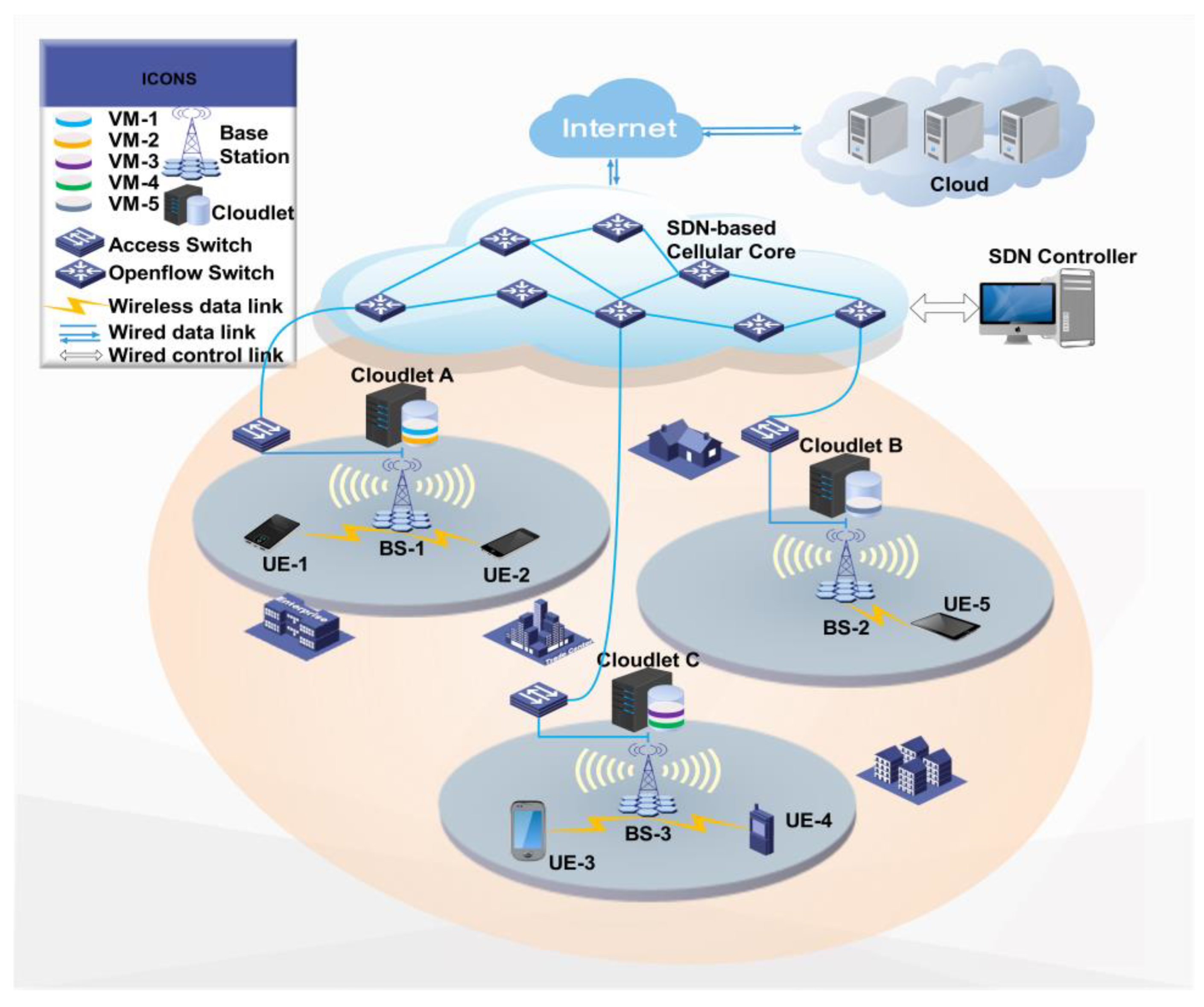
In the cloudlet network (as shown in Figure 1), each cloudlet is deployed near a base station (BS) and is connected to it via high-speed fibers [6]. Therefore, a UD can connect to a nearby BS via a wireless local area network (WLAN) and offload its tasks to the cloudlet where this UD’s VM resides through wired links between BSs. Above the cloudlet layer, a software-defined network (SDN)-based cellular core network is adopted to provide flexible communication routing between BSs and between cloudlets [7,8]. On top of the cellular core network, public data centers provide scalability for VM instantiation. When VMs cannot be instantiated in cloudlets due to capacity constraints, they can be instantiated in public data centers.

Although VMs can be instantiated in cloudlets, the development of physical memory is slower than the increase in memory requirements, and the memory space of each cloudlet is limited, so the number of VMs instantiated in each cloudlet is limited. Memory deduplication is the core of virtualization and is an effective method to address the above issue, as it merges similar data into a single copy using page sharing, thereby reducing the memory requirements of each VM. Memory page sharing is a commonly used memory deduplication technique, in which the hypervisor removes identical memory pages between VMs located at the same position and manages a single page shared among them. When multiple VMs are instantiated in cloudlets, they will share a common memory page set. Depending on the hypervisor in each cloudlet, each cloudlet’s memory utilization will be improved by deleting the same memory pages between VMs and managing VMs to share memory pages of a common memory page set.

However, maximizing memory page sharing between VMs means that VMs tend to be instantiated in a few cloudlets, which prevents the average communication distance between VMs and UDs from being minimized, because VMs cannot communicate with UDs that are evenly distributed across the network with minimal latency. On the contrary, minimizing average communication distance between VMs and UDs means that VMs are instantiated in cloudlets depending on distribution of UDs, which prevents VMs with more of the same memory pages from being instantiated in the same cloudlet.

In this paper, we focus on solving the problem of virtual machine instantiation with the joint optimization of memory sharing and communication distance (VMIJOMSCD), which is a bi-objective optimization problem. This problem requires determining the set of VMs scheduled to be instantiated in each cloudlet while minimizing average communication distance between VMs and UDs and maximizing memory sharing between VMs. Due to the difficulty of obtaining all Pareto solutions of a bi-objective optimization problem in polynomial time, we designed an iterative heuristic algorithm based on the ε-constraint method [9]. This algorithm decomposes the original problem into multiple single-objective optimization subproblems and obtains optimal solutions for the subproblems through iteration calculation. The major contributions of this paper are summarized as follows:

• For the first time, we focus on a new problem of virtual machine instantiation in cloudlet networks, named VMIJOMSCD, and we build a new cloudlet network architecture with memory-shared virtual machines. We formulate the VMIJOMSCD as a bi-objective optimization model.
• In order to obtain representative approximate Pareto solutions in a shorter computation time. We designed an iterative heuristic algorithm, which can obtain relatively accurate solutions in small-scale experimental scenarios. To the best of our knowledge, no heuristic algorithms for solving the VMIJOMSCD problem have been proposed in the research literature to date.
• We investigate the performance of our proposed algorithm by comparing it with the performance of several other benchmark greedy algorithms on real datasets. The experimental results show that compared with other benchmark algorithms, this algorithm has better performance in terms of minimum communication distance and maximum memory sharing.

Our paper is divided into six sections: In Section 2, we review some works related to the field of this article. In Section 3, we give basic system models, including the model of memory sharing between VMs and the model of average communication distance between VMs and UDs. In Section 4, we describe detailed steps of the traditional ε-constraint method and the iterative heuristic algorithm. Then, we evaluate the performance of the proposed algorithm in Section 5. Finally, Section 6 concludes this paper.

2. Related Works

With the increasing popularity of virtualization technology, the multi-objective optimization problem of VM instantiation has received widespread attention. Previous work has explored improving memory sharing between VMs and maintaining low communication distance and latency between UDs and VMs.

2.1. Memory Sharing System

Currently, most research on memory sharing mainly focuses on developing page-sharing systems using content-based page-sharing technology.

Bugnion et al. [10] designed a scalable memory-sharing multiprocessor and proposed a transparent page-sharing technology.

VMWare’s ESX Server has proposed several new memory management mechanisms [11]: Ballooning technology recovers pages from VMs that are considered the least valuable by the operating system. Idle memory tax can improve memory utilization. Content-based page-sharing technology eliminates memory redundancy.

Pan et al. [12] proposed a DAH mechanism that coordinates memory deduplication engines with VM monitoring programs to promote memory sharing between VMs located in the same position while minimizing the performance impact of memory deduplication on running VMs.

Ji et al. [13] proposed STYX, a framework for offloading the intensive operations of these kernel features to SmartNIC (SNIC). STYX first RDMA-copies the server’s memory regions, on which these kernel features intend to operate, to an SNIC’s memory region, exploiting SNIC’s RDMA capability. Subsequently, leveraging SNIC’s compute capability, STYX makes the SNIC CPU perform the intensive operations of these kernel features. Lastly, STYX RDMA-copies their results back to a server’s memory region, based on which it performs the remaining operations of the kernel features.

Ge et al. [14] proposed a memory sharing system, which integrates a mechanism of threshold-based memory overload detection, that is presented for handling memory overload of InfiniBand-networked PMs in data centers. It enables a PM with memory overload to automatically borrow memory from a remote PM with spare memory. Similar to swapping to a secondary memory, i.e., disks, inactive memory pages are swapped to the remote PM with spare memory as a complement to VM live migration and other options for memory tiering, thus handling the memory overload problem.

Wood et al. [15] proposed a memory-sharing-aware VM placement system called Memory Buddies, which avoids memory redundancy by integrating VMs with higher sharing potential on the same host. They also proposed an intelligent VM hosting algorithm to optimize VM placement via real-time migration in response to server workload changes.

2.2. Memory Sharing Problem

The remaining research on memory sharing has focused on studying abstraction problems to achieve certain goals.

He et al. [16] proposed a data routing strategy based on the global BloomFilter, which does not need to maintain all data block fingerprint information, uses superblocks as the data routing unit, maintains the BloomFilter array of the entire deduplication system storage node in the memory of the client server (each row corresponds to one storage node), and maintains the representative fingerprint of the superblock stored using the node, which greatly reduces the memory space occupation. In addition, while maintaining the BloomFilter array, the capacity information of a storage node is also maintained to ensure the load balancing of the storage node.

Rampersaud et al. [17] developed a greedy algorithm to maximize the benefits of a memory-sharing-aware VM deployment, considering only the memory usage of each VM and the memory sharing between VMs.

Rampersaud et al. [18] designed a sharing-aware greedy approximation algorithm to solve the problem of maximizing the benefits of a memory-sharing-aware VM placement in a single-server environment, considering both memory sharing and multiple resource constraints.

Sartakov et al. [19] described Object Reuse with Capabilities (ORC), a new cloud software stack that allows deduplication across tenants with strong isolation, a small TCB, and low overheads. ORC extends a binary program format to enable isolation domains to share binary objects, i.e., programs and libraries, by design. Object sharing is always explicit, thus avoiding the performance overheads of hypervisors with page deduplication. For strong isolation, ORC only shares immutable and integrity-protected objects. To keep the TCB small, object loading is performed using the untrusted guest OS.

Jagadeeswari et al. [20] proposed a modified approach of Memory Deduplication of Static Memory Pages (mSMD) for achieving performance optimization in virtual machines by reducing memory capacity requirements. It is based on the identification of similar applications via Fuzzy hashing and clustering them using the Hierarchical Agglomerative Clustering approach, followed by similarity detection between static memory pages based on genetic algorithm and details stored in a multilevel shared page table; both operations are performed offline, and final memory deduplication is carried out during online,

Wei et al. [21] proposed USM, a build-in module in the Linux kernel that enables memory sharing among different serverless functions based on the content-based page sharing concept. USM allows the user to advise the kernel of a memory area that can be shared with others through the madvise system call, no matter if the memory is anonymous or file-backed.

Jagadeeswari et al. [22] proposed an approach that virtual machines with similar operating systems of active domains in a node are recognized and organized into a homogenous batch, with memory deduplication performed inside that batch, to improve the memory pages sharing efficiency.

Du et al. [23] proposed ESD, an ECC-assisted and Selective Deduplication for encrypted NVMM by exploiting both the device characteristics (ECC mechanism) and the workload characteristics (content locality). First, ESD utilizes the ECC information associated with each cache line evicted from the Last-Level Cache (LLC) as the fingerprint to identify data similarity and avoids the costly hash calculating overhead on the non-duplicate cache lines. Second, ESD leverages selective deduplication to exploit the content locality within cache lines by only storing the fingerprints with high reference counts in the memory cache to reduce the memory space overhead and avoid fingerprints NVMM lookup operations.

2.3. Communication Distance Problem

On the other hand, the studies on reducing communication distance and latency between UDs and VMs mainly focus on designing VM integration strategies.

Sun et al. [24] use cloudlets, software-defined networking, and cellular network infrastructure to bring computing resources to network edge. To minimize the average response time of mobile UDs unloading their workloads to cloudlets, a latency-aware workload offloading strategy is proposed, which assigns the workload of UDs’ applications to appropriate cloudlets.

Genez et al. [25] propose PL-Edge, a latency-aware VM integration solution for mobile edge computing, which dynamically reallocates VMs and network policies in a joint manner to minimize end-to-end latency between UDs and VMs.

Liu et al. [26] study the placement and migration of VMs in mobile edge computing environments and propose a mobile-aware dynamic services placement strategy, which reduces the number of VM migrations by filtering out invalid migration and reduces the overall latency perceived by users.

Sun et al. [27] propose a green cloudlet network architecture, where all cloudlets are powered with green energy and grid energy. To minimize network energy consumption while meeting the low latency requirements between UDs and VMs, VMs are migrated to cloudlets with more green energy generation and less energy demand.

Sun et al. [8] propose the latency-aware VM replica placement algorithm, which places multiple replicas of each VM’s virtual disk in appropriate cloudlets so that when a UD roams away from its VM, the VM can quickly switch to a cloudlet with a shorter communication distance to that UD, avoiding an increase in communication latency between the two. Meanwhile, considering the capacity of each cloudlet, the latency-aware VM switching algorithm is proposed to migrate UDs’ VMs to appropriate cloudlets in each time slot to minimize average communication latency.

2.4. Comparison with Related Works

The above articles propose methods from two perspectives to improve memory sharing between VMs or reduce communication latency and distance between UDs and VMs. However, no article considers solving these two important problems at the same time. Compared to the development of memory sharing systems or virtual machine scheduling strategies, this article focuses more on the research of abstract theoretical problems. To our best knowledge, this is the first article to consider simultaneously minimizing average communication distance between UDs and VMs and maximizing memory sharing between VMs when instantiating VMs.

We use

Table 1. Comparison with related works.

Article	Publication Time	Network Environment	Objectives	Whether to Propose a System	Experimental Scenario	Whether User-Dedicated VMs are Considered	Dataset
Memory Resource Management in VMware ESX Server [11]	2002	General Server Network	Maximize hardware resource reuse between virtual machines	YES	Multiple VMs on a single server	NO	Real dataset
Memory Buddies: Exploiting Page Sharing for Smart Colocation in Virtualized Data Centers [15]	2009	Data Center Network	Maximize memory sharing among virtual machines	YES	Multiple VMs on multiple servers	NO	Real dataset
Hypervisor Support for Efficient Memory Deduplication [12]	2011	General Server Network	Minimize the performance impact of memory deduplication on running virtual machines	YES	Multiple VMs on a single server	NO	Simulated dataset
STYX: Exploiting SmartNIC Capability to Reduce Datacenter Memory Tax [13]	2023	General Server Network	Deploying memory deduplication with minimal interference to the running applications.	YES	Multiple VMs on a single server	NO	Simulated dataset
Memory Sharing for Handling Memory Overload on Physical Machines in Cloud Data Centers [14]	2023	Cloud Computing Network	Minimize the probability of server memory overload.	YES	Multiple VMs on multiple servers	NO	Simulated dataset
Memory Deduplication on ServerlessSystems [21]	2021	Serverless Network	Maximize memory sharing	NO	Multiple VMs on a single server	NO	Simulated dataset
An Approximation Algorithm for Sharing-AwareVirtual Machine Revenue Maximization [18]	2021	Cloud Computing Network	Maximize revenue by deploying sharing-aware virtual machines	NO	Multiple VMs on multiple servers	NO	Real dataset
Homogeneous Batch Memory Deduplication Using Clustering of Virtual Machines [22]	2022	Cloud Computing Network	Maximize memory sharing among virtual machines of the same user.	NO	Multiple VMs on a single server	NO	Simulated dataset
Research on Global BloomFilter-Based Data Routing Strategy of Deduplication inCloud Environment [16]	2023	Cloud Computing Network	Ensuring node load balancing while avoiding a significant drop-in memory deduplication rate	NO	Single VM on a single server	NO	Simulated dataset
ORC: Increasing Cloud Memory Density via Object Reuse with Capabilities [19]	2023	Cloud Computing Network	Maximize memory sharing while ensuring isolation of tenants and their workloads.	NO	Multiple VMs on a single server	NO	Real dataset
Optimization of Virtual Machine PerformanceUsing Fuzzy Hashing and Genetic-Algorithm-basedMemory Deduplication of Static Pages [20]	2023	Cloud Computing Network	Maximize memory deduplication	NO	Multiple VMs on a single server	NO	Simulated dataset
ESD: An ECC-assisted and Selective Deduplicationfor Encrypted Non-Volatile Main Memory [23]	2023	General Server Network	Maximize the efficiency of memorydeduplication	NO	Multiple VMs on a single server	NO	Simulated dataset
Joint Optimization of Memory Sharing and Communication Distance for Virtual Machine Instantiation in Cloudlet Networks		Cloudlet Network	Maximize memory sharing and minimize communication distance	YES	Multiple VMs on multiple servers	YES	Real dataset

to present the differences between this article and related works more clearly.

3. System Model and Problem Statement

We consider a wireless metropolitan area network consisting of multiple BSs located at different positions. Therefore, the network can be represented using a fully undirected connected graph $G=\left(V,E\right)$, where $V=\left\{v_1,v_2,\dots ,v_n\right\}$ is the set of BSs. The fiber optic communication links between any two BS $v_i\left(v_i\in V\right)$ and $v_j\left(v_j\in V\right)$ constitute the set of links, $E=\left\{e\left(v_i,v_j\right)\right|v_i,v_j\in V\}$. We use $d_{ij}$ to represent distance between BSs $v_i$ and $v_j$. If there is a direct link between $v_i$ and $v_j$, then $d_{ij}$ equals the Euclidean distance between $v_i$ and $v_j$, which is the length of edge $e\left(v_i,v_j\right)$. Otherwise, $d_{ij}$ represents the shortest multi-hop cumulative distance from $v_i$ to $v_j$. For BS $v_i$, we assign $w\left(v_i\right)$ to represent the expected number of user requests accessing the Internet through this BS. $w\left(v_i\right)$ can be calculated based on historical UDs’ access data through this BS. The measurement of expected user requests is not the focus of this paper, so we only consider $w\left(v_i\right)$ as a weight on $v_i$.

Assuming $Q$, $T$, and $O$ represent the sets of UDs, VMs, and cloudlets, respectively. For each cloudlet $o\left(o\in O\right)$, we assume that it contains three types of resources: memory, CPU, and storage, and we use $C_o^m$, $C_o^u$, and $C_o^s$ to represent the memory, CPU, and storage capacity of $o$. In this paper, we assume that each cloudlet is deployed near a BS. The cloudlets in set $O$ are deployed near $\left|O\right|$ BSs in set $V$. Therefore, we further assume that $\left|O\right|\ll \left|V\right|$. Each cloudlet in set $O$ can be connected to any BS through inter-BS links. We use $l_{ov}$ to represent the communication delay between BS $v$ and cloudlet $o$. This value is proportional to $d_{ov}$, i.e., $l_{ov}=0.016d_{ov}+22.3$, and ref. [28] and $l_{ov}$ can be measured and recorded using the SDN controller [29,30].

For each UD $q\left(q\in Q\right)$, we assume that a dedicated VM $t_q\left(t_q\in T\right)$ is assigned to it, which runs the same operating system as $q$, runs application components of $q$, and provides dedicated services for $q$. Each VM will be allocated and instantiated in a cloudlet in $O$, so $\left|Q\right|$ VMs waiting to be instantiated constitute $T$, that is, $\left|Q\right|=\left|T\right|$. Each VM requires a given number of three types of resources when instantiated, which are represented by $r_q^m$, $r_q^u$, and $r_q^s$, respectively, for the memory resources, CPU resources, and storage resources required for $t_q$ instantiation. Multiple VMs instantiated in the same cloudlet will share memory resources, CPU resources, and storage resources of that cloudlet and are managed by the hypervisor in that cloudlet. The hypervisor manages reclamation of memory pages and converts memory pages between the cloudlet and VMs. Pan et al. [12] proposed to use an external mechanism to coordinate works of hypervisors. We assume that an external mechanism is used to assist the hypervisor running on each cloudlet to manage a unified memory page library $\tilde{\Pi }$, which contains all the memory pages required when VMs are instantiated. To identify memory pages in $\tilde{\Pi }$, we use ${\pi }^i$ to represent the $i$-th memory page in $\tilde{\Pi }$. We assume that $\tilde{\Pi }$ contains $\mathrm{Z}$ pages, that is, $\tilde{\Pi }={\cup }_{i=1}^{\mathrm{z}}\left\{{\pi }^i\right\}$, and let ${\pi }_q^i$ be the $i$-th memory page required when $t_q$ is instantiated.

For the convenience of formulating the two objectives proposed in this paper, the following decision variables are given: Let $x_{qo}$ be a binary variable used to represent whether $t_q$ is instantiated on $o$. When $x_{qo}$=1, it indicates that $t_q$ is instantiated on $o$, otherwise, $x_{qo}=0$. Let $y_{qvo}$. be a binary variable used to represent whether the VM of $q$ is instantiated on $o$ when $q$ is in the coverage area of $v$. When $y_{qvo}=1$, it indicates that $q$ is in the coverage area of $v$, and the VM of $q$ is instantiated on $o$. Otherwise, $y_{qvo}=0$.

In the following, we will introduce the model of memory sharing between VMs and the model of average communication distance between VMs and UDs.

The notation used in the paper is presented in

Table 2. Notation.

Expression	Description
$V$	Set of base stations
$v_i\left(v_i\in V\right)$	Base station with index $i$
$E$	Set of links
$e\left(v_i,v_j\right)$	Link $\mathrm{between} v_i\left(v_i\in V\right)$ and $v_j\left(v_j\in V\right)$
$d_{ij}$	Link $\mathrm{distance} \mathrm{between} v_i$$\mathrm{and} v_j$
${\tilde{d}}_{ij}$	$\mathrm{Euclidean} \mathrm{distance} \mathrm{between} v_i$$\mathrm{and} v_j$
$w\left(v_i\right)$	$\mathrm{Expected} \mathrm{number} \mathrm{of} \mathrm{user} \mathrm{requests} \mathrm{accessing} \mathrm{the} \mathrm{Internet} \mathrm{through} v_i$
$Q$	Set of UDs
$T$	Set of VMs
$O$	Set of cloudlets
$C_o^m$	$\mathrm{Memory} \mathrm{capacity} \mathrm{of} \mathrm{cloudlet} o$
$C_o^u$	$\mathrm{CPU} \mathrm{capacity} \mathrm{of} \mathrm{cloudlet} o$
$C_o^s$	$\mathrm{Storage} \mathrm{capacity} \mathrm{of} \mathrm{cloudlet} o$
$l_{ov}$	$\mathrm{Communication} \mathrm{delay} \mathrm{between} \mathrm{BS} v$$\mathrm{and} \mathrm{cloudlet} o$
$t_q\left(t_q\in T\right)$	$\mathrm{A} \mathrm{dedicated} \mathrm{VM} \mathrm{for} \mathrm{UD} q\left(q\in Q\right)$
$r_q^m$	$\mathrm{Memory} \mathrm{resources} \mathrm{required} \mathrm{for} t_q$ instantiation
$r_q^u$	$\mathrm{CPU} \mathrm{resources} \mathrm{required} \mathrm{for} t_q$ instantiation
$r_q^s$	$\mathrm{Storage} \mathrm{resources} \mathrm{required} \mathrm{for} t_q$ instantiation
$\tilde{\Pi }$	Unified memory page library
${\pi }^i$	Memory page $i$
${\pi }_q^i$	$\mathrm{The}$ i-$\mathrm{th} \mathrm{memory} \mathrm{page} \mathrm{required} \mathrm{when} t_q$ is instantiated
$x_{qo}$	$\mathrm{A} \mathrm{binary} \mathrm{variable} \mathrm{used} \mathrm{to} \mathrm{represent} \mathrm{whether} t_q$$\mathrm{is} \mathrm{instantiated} \mathrm{on} o$
$y_{qvo}$	$\mathrm{A} \mathrm{binary} \mathrm{variable} \mathrm{used} \mathrm{to} \mathrm{represent} \mathrm{whether} \mathrm{the} \mathrm{VM} \mathrm{of} q$$\mathrm{is} \mathrm{instantiated} \mathrm{on} o$$\mathrm{when} q$$\mathrm{is} \mathrm{in} \mathrm{the} \mathrm{coverage} \mathrm{area} \mathrm{of} v$
$Z_{jk}^{\theta }$	$\mathrm{The} \mathrm{metric} \mathrm{of} \mathrm{VM} t_j$$\mathrm{instantiated} \mathrm{in} \mathrm{the} \mathrm{cloudlet} o_k$$\mathrm{at} \mathrm{the} \theta$-th iteration
$\Psi$	$\mathrm{Size} \mathrm{of} \mathrm{a} \mathrm{memory} \mathrm{page} \mathrm{that} \Psi =10\mathrm{MB}$
${\mathcal{T}}_k^{\mathcal{H}1}$	$\mathrm{VM} \mathrm{set} \mathrm{that} \mathrm{planned} \mathrm{to} \mathrm{be} \mathrm{instantiated} \mathrm{in} o_k$, aiming to maximize memory sharing among VMs
${\mathcal{T}}_k^{\mathcal{H}2}$	$\mathrm{VM} \mathrm{set} \mathrm{that} \mathrm{planned} \mathrm{to} \mathrm{be} \mathrm{instantiated} \mathrm{in} o_k$, aiming to minimize average communication distance between VMs and UDs
$\mathcal{P}\left(T\right)$	$\mathrm{Power} \mathrm{set} \mathrm{of} T$
$I$	$\mathrm{Subset} \mathrm{of} \mathcal{P}\left(T\right)$
${\sigma }_I$	$\mathrm{The} \mathrm{number} \mathrm{of} \mathrm{non}-\mathrm{repeated} \mathrm{pages} \mathrm{shared} \mathrm{among} \mathrm{VMs} \mathrm{in} I$$, \mathrm{when} \left|I\right|$$=1, {\sigma }_I$$\mathrm{represents} \mathrm{the} \mathrm{number} \mathrm{of} \mathrm{memory} \mathrm{pages} \mathrm{corresponding} \mathrm{to} r_q^m$$\mathrm{of} t_q$$\mathrm{in} I$$, \mathrm{i}.\mathrm{e}., {\sigma }_q=r_q^m/\Psi$
$p_{qv}$	$\mathrm{The} \mathrm{probability} \mathrm{of} q$$\mathrm{appearing} \mathrm{in} \mathrm{the} \mathrm{coverage} \mathrm{range} \mathrm{of} v$
$I$	$\mathrm{Subset} \mathrm{of} \mathcal{P}\left(T\right)$
$\mathcal{F}$	Set of Pareto front solutions
$a_{jk}^0$	$\mathrm{Shared} \mathrm{potential} \mathrm{of} t_j$$\mathrm{with} \mathrm{all} \mathrm{VMs} \mathrm{in} T$
$a_{jk}^i$	$\mathrm{Same} \mathrm{memory} \mathrm{pages} \mathrm{between} t_j$$\mathrm{and} \mathrm{the} \mathrm{instantiated} \mathrm{VMs} \mathrm{in} o_k$$\mathrm{in} i$-th iteration
${\eta }_i\left(f_i^k\right)$	$\mathrm{Optimality} \mathrm{of} \mathrm{the} k$$\mathrm{-th} \mathrm{solution} \mathrm{on} \mathrm{the} i$-th objective
${\eta }^k$	$\mathrm{Preference} \mathrm{value} \mathrm{of} \mathrm{the} k$-th solution
$a_{jk}^0$	$\mathrm{Shared} \mathrm{potential} \mathrm{of} t_j$$\mathrm{with} \mathrm{all} \mathrm{VMs} \mathrm{in} T$
UP	Ratio of the selected UDs to the total number of UDs
CP	Ratio of the selected BSs to the total number of BSs
SP	Weights of memory sharing among VMs
LP	Weights of average communication distance between VMs and UDs

3.1. Memory Sharing Model

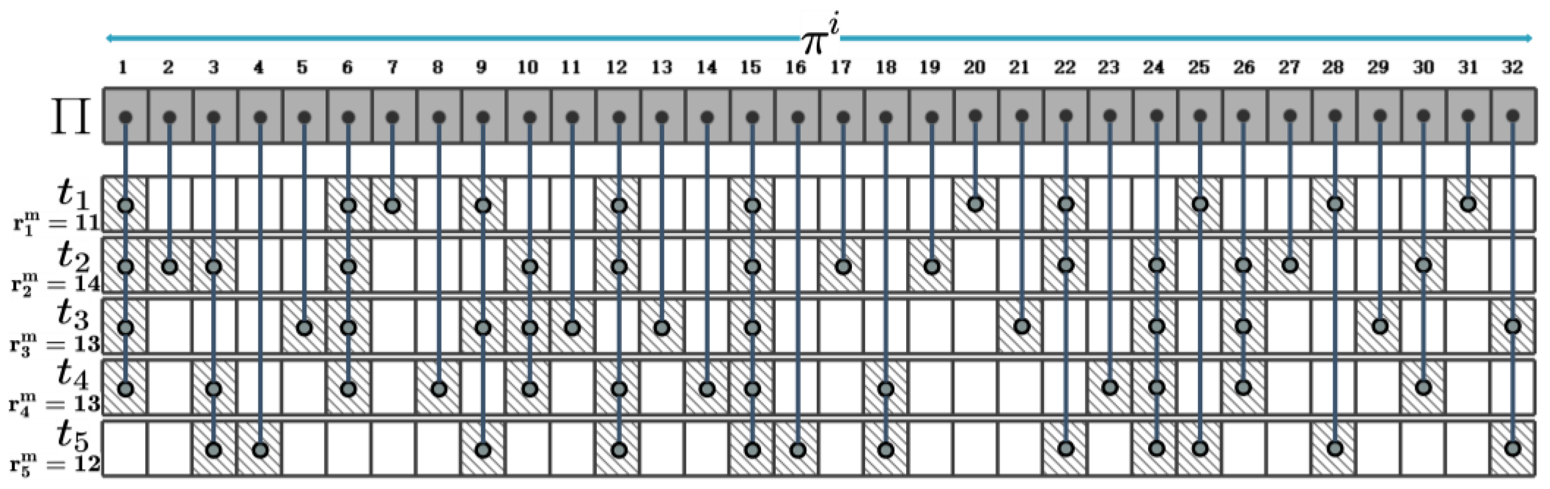
To provide a more detailed explanation of memory page sharing between VMs, we present an example. Suppose there are four VMs $t_1,t_2,t_3,$ and $t_4$ that need to be instantiated in two cloudlets $o_1$ and $o_2$. $t_5$ has already been instantiated in $o_2$, and its memory pages have been hosted in the memory space of $o_2$. We assume that $t_1,t_2,t_3,t_4, \mathrm{and} t_5$ have requested a total of 32 different memory pages, which are represented by ${\pi }^1,{\pi }^2,\dots ,{\pi }^{32}$. Figure 2 shows the details of the memory pages required for the instantiation of $t_1,t_2,t_3,t_4, \mathrm{and} t_5$. As shown in Figure 2, $t_1$ requires a total of 11 memory pages (the shaded boxes in first row correspond to the memory pages requested by $t_1$). The thick vertical lines connecting shaded boxes indicate the same pages between VMs. For example, page ${\pi }^{12}$ is required for the instantiation of $t_1,t_2,t_4,$ and $t_5$, so the shaded boxes corresponding to ${\pi }^{12}$ in $t_1,t_2,t_4,$ and $t_5$ are connected by a thick vertical line, indicating that $t_1,t_2,t_4,$ and $t_5$ can share ${\pi }^{12}$ when they are instantiated in the same cloudlet.

According to Figure 2, $t_5$ has different numbers of identical memory pages with $t_1,t_2,t_3,$ and $t_4$. Therefore, in order to obtain a VM instantiation plan that maximizes memory sharing among VMs, it is necessary to consider the impact of the number of identical memory pages between VMs on memory sharing when allocating and instantiating $t_1,t_2,t_3,t_4$ in $o_1$ and $o_2$. To maximize memory sharing among VMs, we use an iterative method to select one VM at a time from the VMs to be instantiated and determine which cloudlet it will be instantiated in. To this end, we design a metric that considers memory sharing between the selected VM and the VMs instantiated in each cloudlet, as well as the proportion of resources occupied by this VM in a corresponding cloudlet. After determining the allocation position of a VM each time, we recalculate the metrics of remaining VMs and adjust iteration order accordingly. The metric $Z_{jk}^{\theta }$ of VM $t_j$ instantiated in the cloudlet $o_k$ at the $\theta$-th iteration is defined as follows:

$$Z_{jk}^{\theta }=\frac{a_{jk}^{\theta }+{\overline{a}}_{jk}^{\theta }}{\sqrt{\frac{r_j^s}{C_k^s}+\frac{r_j^u}{C_k^u}+\frac{r_j^m-a_{jk}^{\theta }+1}{C_k^m}}}$$

(1)

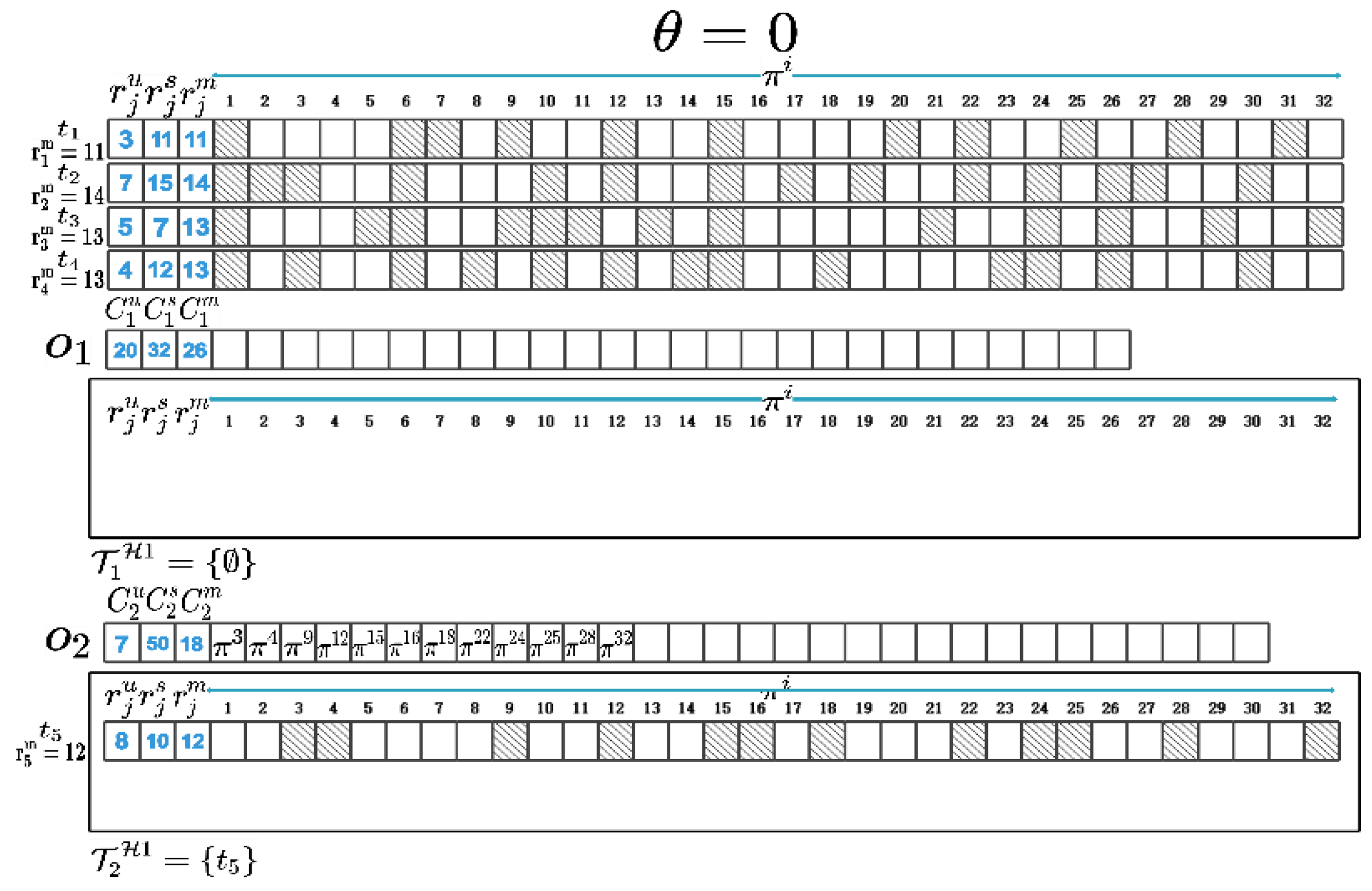
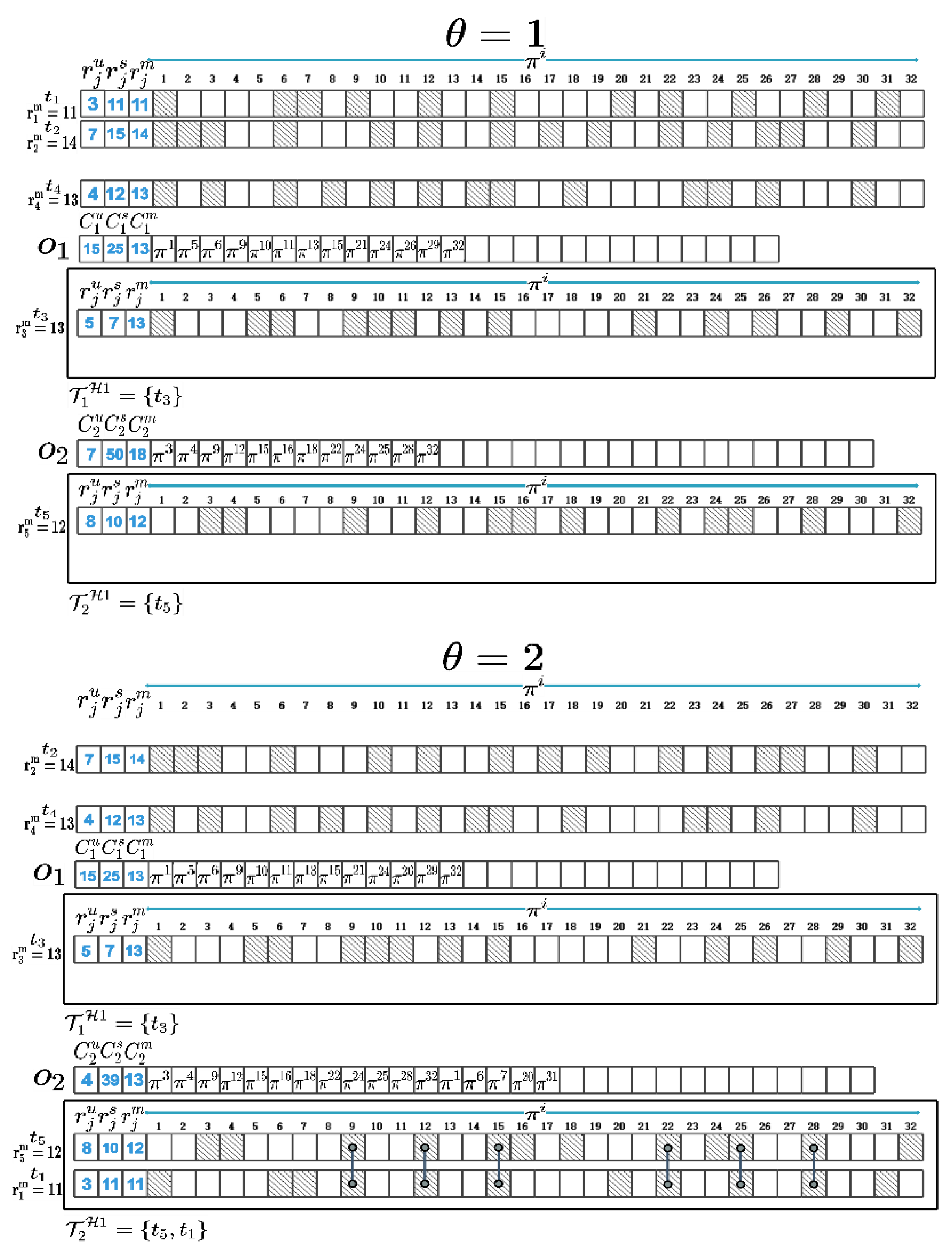
We use $\Psi$ to represent size of a memory page and assume that $\Psi =10\mathrm{MB}$. The $a_{jk}^{\theta }$ in (1) represents the product of $\Psi$ and the number of the same memory pages between $t_j$ and the VM set ${\mathcal{T}}_k^{\mathcal{H}1}$ that planned to be instantiated in $o_k$ in the $\theta$ iteration. If ${\mathcal{T}}_k^{\mathcal{H}1}$ is an empty set, $a_{jk}^{\theta }$ represents the memory sharing potential between $t_j$ and all the VMs to be instantiated in the $\theta$ iteration. ${\overline{a}}_{jk}^{\theta }$ is used to represent the minimum number of different memory pages between $t_j$ and the VM set ${\mathcal{T}}_z^{\mathcal{H}1}\left(o_z\in O/o_k\right)$ instantiated in the cloudlets other than $o_k$ in the $\theta$ iteration, multiplied by $\Psi$. After determining where a VM will be instantiated in, the memory pages of this VM will be compared with the memory pages hosted in the corresponding cloudlet’s memory space. The memory pages requested by this VM but not yet hosted in the corresponding cloudlet will be added to this cloudlet’s memory space. To maximize memory sharing between VMs, we calculate metric indicators of $t_1,t_2,t_3,t_4$ with $o_1$ and $o_2$ in turn, and we select the VM and cloudlet with the maximum metric indicator. In the first iteration, $Z_{31}^1$ is greater than the other $Z_{jk}^1$, so when $\theta =1$, $t_3$ should be instantiated in $o_1$. Then, we compare the memory pages of $t_3$ with those hosted in $o_1$ and add different memory pages to $o_1$’s memory space. Next, we add $t_3$ to ${\mathcal{T}}_1^{\mathcal{H}1}$, update $\theta$, and recalculate $Z_{jk}^{\theta }$ for remaining VMs with corresponding cloudlets. Repeat the above process until $t_1,t_2,t_3,$ and $t_4$ are all allocated and instantiated in $o_1$ and $o_2$. At this point, we can obtain the VM instantiation plan ${\mathcal{T}}_1^{\mathcal{H}1}$ and ${\mathcal{T}}_2^{\mathcal{H}1}$ and maximize memory sharing between $t_1,t_2,\dots ,t_5$. Figure 3 shows a partial process diagram of VM allocation and instantiation as well as the three types of resource capacity changes of $o_1$ and $o_2$.

In order to maximize memory sharing between VMs, we represent the objective function $f_1$ as the following:

$$f_1=\max {\displaystyle \sum }_{o\in O}({\displaystyle \sum }_{q\in Q}{x}_{qo}{r}_q^m-\left({\displaystyle \sum }_{I\in \mathcal{P}\left(T\right)}{(-1)}^{\left(\left|I\right|+1\right)}{\sigma }_I{\displaystyle \prod }_{q\in I}{x}_{qo})\mathsf{\Psi }\right)$$

(2)

$$\mathrm{s}.\mathrm{t}. \forall q\in Q,{\displaystyle \sum }_{o\in O}{x}_{qo}=1,$$

(3)

$$\forall o\in O,\left({\displaystyle \sum }_{I\in \mathcal{P}\left(T\right)}{(-1)}^{\left(\left|I\right|+1\right)}{\sigma }_I{\displaystyle \prod }_{q\in I}{x}_{qo}\right)\mathsf{\Psi }\le C_o^m,$$

(4)

$$\forall o\in O,{\displaystyle \sum }_{q\in Q}{r}_q^u{x}_{qo}\le C_o^u,$$

(5)

$$\forall o\in O,{\displaystyle \sum }_{q\in Q}{r}_q^s{x}_{qo}\le C_o^s,$$

(6)

$$\forall q\in Q \forall o\in O,x_{qo}\in \left\{0,1\right\}.$$

(7)

$\mathcal{P}\left(T\right)$ represents power set of $T$, $I$ represents a subset of $\mathcal{P}\left(T\right)$, and ${\sigma }_I$ represents the number of non-repeated pages shared among VMs in $I$.Taking $t_1,t_2,\dots ,t_5$ shown in previous text as an example, suppose the set $\tilde{T}$ consisting of $t_1,t_3,$ and $t_5$ is to be instantiated in the cloudlet $o$. We use $\mathcal{P}\left(\tilde{T}\right)$ to denote the power set of $\left\{t_1,t_3,t_5\right\}$ and $I$ to denote the element set of $\mathcal{P}\left(\tilde{T}\right)$. For $I=\left\{t_1,t_3\right\}$, there are four pages ${\pi }^1,{\pi }^6,{\pi }^9,$ and ${\pi }^{15}$ shared by $t_1$ and $t_3$, so ${\sigma }_I=4$ in this case. When $\left|I\right|$ = 1, ${\sigma }_I$ represents the number of memory pages corresponding to $r_q^m$ of $t_q$ in $I$, i.e., ${\sigma }_q=r_q^m/\mathsf{\Psi }$. Equation (3) requires that each VM can only be instantiated in a cloudlet.

By removing duplicate pages from all memory pages requested by $t_1,t_3,$ and $t_5$, we can obtain the non-repeating set of memory pages, which is managed by $\tilde{\Pi }$ and shared by VMs in $\tilde{T}$. When $t_1,t_3,$ and $t_5$ are instantiated in the same cloudlet $o$, 23 different memory pages are required. Therefore, $\tilde{\Pi }$ needs to manage at least these 23 different memory pages, and the memory capacity of $o$ can accommodate these 23 memory pages so that $t_1,t_3,$ and $t_5$ can be instantiated in $o$. In most cases, the set of VMs to be instantiated in each cloudlet is a subset of all the VMs to be instantiated, selected based on the memory capacity of that cloudlet. Therefore, (4) ensures that the sum of memory resource required by the VMs instantiated in each cloudlet is less than the memory capacity of that cloudlet while considering recycling memory through memory page sharing.

Equations (5) and (6), respectively, require that the sum of CPU and storage resources required by the VMs instantiated in each cloudlet is less than the CPU and storage capacity of that cloudlet. Equation (7) means that $x_{qo}\left(q\in Q,o\in O\right)$ is a binary variable.

3.2. Communication Distance Model

Due to the frequent roaming of UDs, the duration of UDs accessing the Internet through different BSs is different, so the frequency of UDs appearing in the coverage area of each BS is different. If a UD’s VM is instantiated in a cloudlet near the BS, which this UD has never accessed, it is not beneficial for communication between this UD and its VM. The communication latency between a UD and its VM mainly depends on the communication distance between the two [28]. Minimizing the average communication distance between VMs and UDs can ensure that VMs and UDs that frequently appear in different BSs’ coverage areas can always communicate with low latency. Therefore, each VM should be instantiated in the cloudlet with the minimum average communication distance to BSs where its UD frequently accesses.

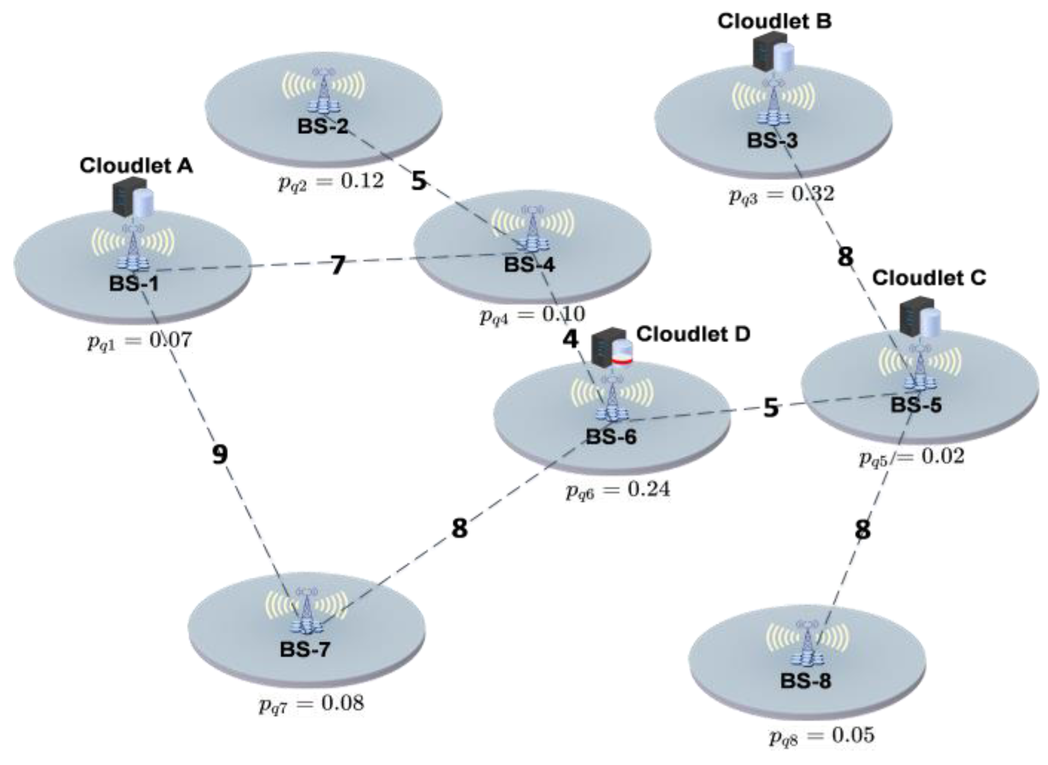
For example, let us assume a cloudlet network topology as shown in Figure 4. There are eight randomly distributed BSs in the area, with cloudlets located near four of them. In order to demonstrate the impact of the average communication distance on the instantiation of VMs, we randomly generate links between any two BSs instead of using the SDN-based cellular core network, and the numbers on the links represent the relative length of the links. We assume a UD $q$’s VM $t_q$ needs to be instantiated in a cloudlet and assume the probability of $q$ appearing in the coverage range of BS $v$ is $p_{qv}$, where $v=1,2, \dots ,8$. As shown in Figure 4, generally, $t_q$ should be instantiated in the cloudlet B because $p_{q3}$ is greater than $p_{q1},p_{q5},$ and $p_{q6}$. This means $q$ often accesses the Internet through BS-3. However, instantiating $t_q$ in the cloudlet B does not minimize the average communication distance between $q$ and $t_q$. On the contrary, instantiating $t_q$ in the cloudlet D can achieve this. This is because the average communication distance between cloudlet B and other BSs is relatively large. If $t_q$ is instantiated in cloudlet B, when $q$ appears in the coverage range of other BSs, the communication distance between $q$ and $t_q$ is large, which will cause a large communication delay between them. On the other hand, the average communication distance between cloudlet D and other BSs is relatively small. When $q$ appears in the coverage range of other BSs, the communication distance between $q$ and $t_q$ is small. Therefore, we conclude that the value of $p_{qv}$ is not the only determining factor affecting the instantiation of VMs, and the average communication distance will also affect the instantiation of VMs.

In order to minimize average communication distance between UDs and VMs, we represent the objective function $f_2$ as the following:

$$f_2=\min {\displaystyle \sum }_{q\in Q}{\displaystyle \sum }_{v\in V}{\displaystyle \sum }_{o\in O}{p}_{qv}{d}_{ov}{y}_{qvo}$$

(8)

$$\mathrm{s}.\mathrm{t}.\forall q\in Q,{\displaystyle \sum }_{o\in O}{x}_{qo}=1,$$

(9)

$$\forall o\in O,\left({\displaystyle \sum }_{I\in \mathcal{P}\left(T\right)}{(-1)}^{\left(\left|I\right|+1\right)}{\sigma }_I{\displaystyle \prod }_{q\in I}{x}_{qo}\right)\mathsf{\Psi }\le C_o^m,$$

(10)

$$\forall o\in O,{\displaystyle \sum }_{q\in Q}{r}_q^u{x}_{qo}\le C_o^u,$$

(11)

$$\forall o\in O,{\displaystyle \sum }_{q\in Q}{r}_q^s{x}_{qo}\le C_o^s,$$

(12)

$$\forall q\in Q \forall o\in O,x_{qo}\in \left\{0,1\right\},$$

(13)

$$\forall q\in Q\forall v\in V,{\displaystyle \sum }_{o\in O}{y}_{qvo}=1,$$

(14)

$$\forall q\in Q\forall v\in V\forall o\in O,y_{qvo}\le x_{qo},$$

(15)

$$\forall q\in Q\forall v\in V\forall o\in O,y_{qvo}\in \left\{0,1\right\}.$$

(16)

$p_{qv}$ is the probability that $q$ appears in the coverage area of $v$ during the period $\mathsf{\Delta }$, and $d_{ov}$ is the communication distance between $o$ and $v$. The objective function $f_2$ must satisfy partial constraints together with the objective function $f_1$, that is, $\left(9\right)$–$\left(13\right)$. Equation (14) requires that when a UD appears in any BS’s coverage range, this UD’s VM should be instantiated on a cloudlet. Equation (15) requires that $y_{qvo}$ can only be set to 1 when the $q$’s VM is instantiated in cloudlet $o$, i.e., $x_{qo}$ = 1; otherwise, $y_{qvo}$ can only be set to 0 when $x_{qo}$ = 0. Equation (16) indicates that $y_{qvo}(q\in Q,o\in O,v\in V$) is a binary variable.

4. Proposed Solution

This section introduces the algorithm proposed in this paper. First, we introduce the traditional ε-constraint method, then we provide a detailed introduction to the iterative heuristic algorithm.

4.1. Traditional ε-Constraint Method

We will now introduce multi-objective optimization problems and the traditional ε-constraint method. Taking the minimization problem as an example, a multi-objective optimization problem can be represented as the following:

$$\min f\left(x\right)=\min \left(f_1\left(x\right),f_2\left(x\right),\dots ,f_z\left(x\right)\right)$$

(17)

$x\left(x\in X\right)$ is decision variable, and $X$ is solution space. $f_1\left(x\right), f_2\left(x\right),\dots ,f_z\left(x\right)$ are the $z$ objective functions, and $F=\left\{f\left(x\right)\mid x\in X\right\}$ refers to objective function vector space.

So far, several methods have been developed to deal with the multi-objective optimization problems, among which the weighted sum method and the ε-constraint method are two commonly used methods for solving multi-objective optimization problems. The former combines all objective functions using a weighted sum formula, thereby transforming the multi-objective optimization problem into a single-objective optimization problem. The quality of solutions obtained by this method largely depends on the weights of each objective. The latter method selects one of the objectives as a preferred optimization target and transforms the other objectives into additional constraints, and by means of this transformation, the multi-objective optimization problem is converted into multiple single-objective optimization problems. Then, by iteratively solving a series of single-objective optimization problems, the Pareto front can be derived. This method can overcome the disadvantages of the weighted sum method due to unreasonable weight allocation [31]. The ε-constraint method was first proposed by Haimes et al. [9] and has been greatly improved over the years. Therefore, this paper designs an algorithm based on the ε-constraint method.

We will now introduce the principle of the ε-constraint method for bi-objective optimization problems. Without loss of generality, we assume a bi-objective optimization function as the following:

$$\min f\left(x\right)=\min \left(f_1\left(x\right),f_2\left(x\right)\right)$$

(18)

We choose $f_2\left(x\right)$ as the main optimization objective and transform $f_1\left(x\right)$ into an additional constraint. At this point, the bi-objective problem can be transformed into the following single-objective optimization problem $P^{\prime }$:

$$P^{\prime }:\min f_2\left(x\right)$$

(19)

$$\mathrm{s}.\mathrm{t}. f_1\left(x\right)\le \epsilon ,x\in X.$$

(20)

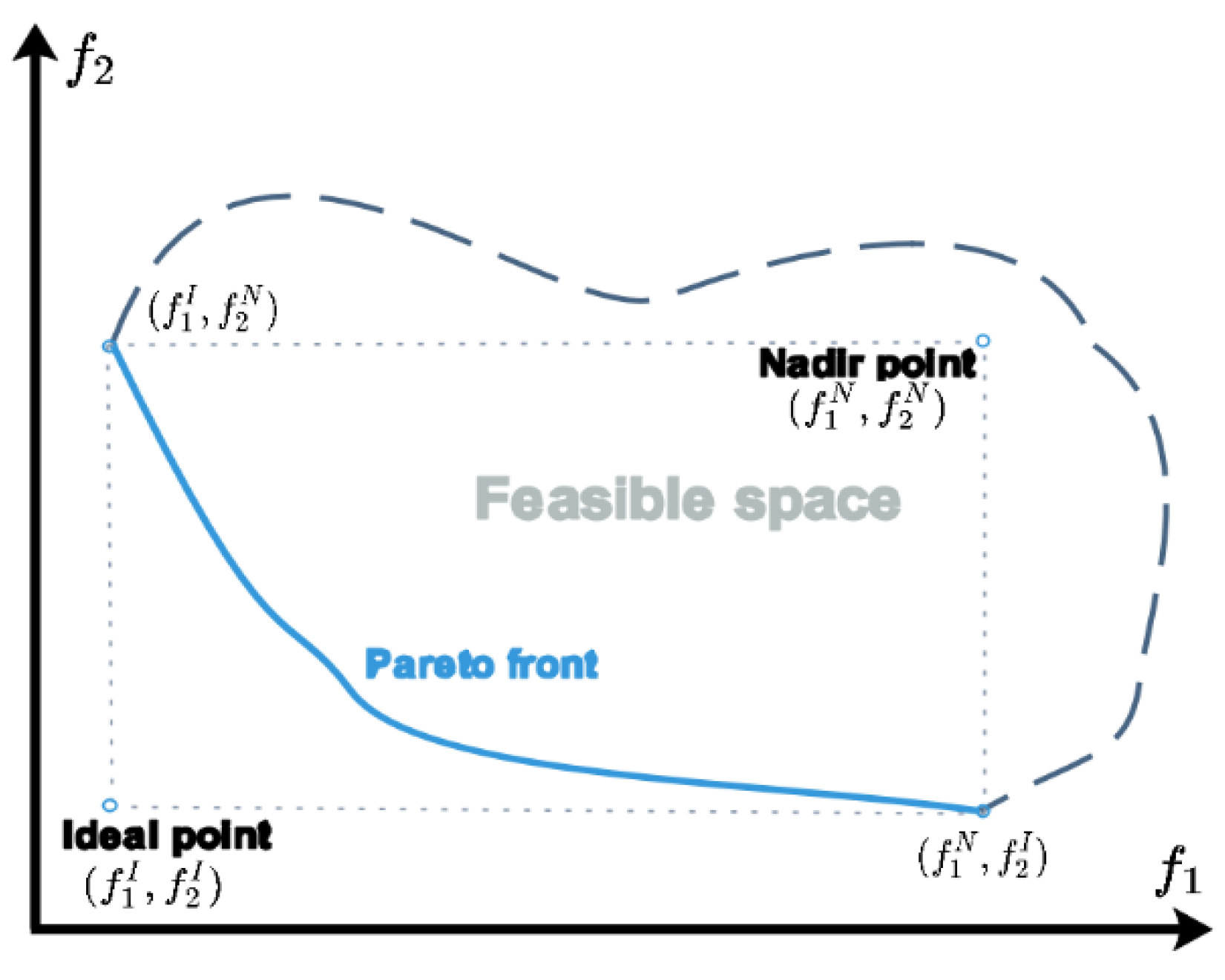
$f_1\left(x\right)$ is limited by $\epsilon$. In order to obtain an effective solution, it is necessary to select an appropriate range for $\epsilon$. The interval of $\epsilon$ can be determined based on the ideal point and the nadir point in objective function vector space, where $\left(f_1^I,f_2^I\right)$ represents the ideal point, $\left(f_1^N,f_2^N\right)$ represents the nadir point, and values of $f_1^I, f_2^I,f_1^N and f_2^N$ can be obtained by solving the following four single-objective optimization problems, respectively: $f_1^I=\min \left\{f_1\left(x\right)\right|x\in X\}, f_2^I=\min \{f_2\left(x\right)|x\in X\}, f_1^N=min\left\{f_1\left(x\right)\right|f_2\left(x\right)=f_2^I ,x\in X\}, f_2^N=\min \{f_2\left(x\right)|f_1\left(x\right)=f_1^I ,x\in X\},$ where range of $\epsilon$ is defined as $\left[f_1^I,f_1^N\right]$. Figure 5 shows positions of the ideal point and the nadir point in objective function vector space. The Pareto front is contained between the ideal point and the nadir point.

In this method, the objective function vector of the first solution is set as $\left(f_1^N,f_2^I\right)$ and then let $\epsilon =f_1^N-\delta$, where $\delta$ is a sufficiently small positive number, and we set it to 1. We then solve $P^{\prime }$ and obtain the current optimal solution $x^{*}$, which is the second solution in the Pareto front and corresponds to objective function vector $\left(f_1\left(x^{*}\right),f_2\left(x^{*}\right)\right)$. Next, let $\epsilon =f_1\left(x^{*}\right)-\delta$ and repeat the above process until $\epsilon \le f_1^I$. Finally, we remove dominated solutions from a solution set and keep all non-dominated solutions to obtain the Pareto front $\mathcal{F}$. Detailed steps of this method are shown in Algorithm 1.

Algorithm 1 ε-Constraint Method

1: $\mathrm{Calculate} f_1^I,f_2^I,f_1^N, \mathrm{and} f_2^N \mathrm{to} \mathrm{obtain} \left(f_1^I,f_2^I\right) \mathrm{and} \left(f_1^N,f_2^N\right).$ 2: $\mathrm{Set} \mathcal{F}=\left\{\left(f_1^N,f_2^I\right)\right\},\epsilon =f_1^N-\delta .$ 3: Solve $P^{\prime }$ and obtain the optimal solution $x^{*}$. Incorporate the objective vector corresponding to $x^{*}$, i.e., $\left(f_1\left(x^{*}\right),f_2\left(x^{*}\right)\right)$, into $\mathcal{F}$. 4: Set $\epsilon =f_1\left(x^{*}\right)-\delta .$ 5: $\mathrm{If} \epsilon \ge f_1^I, \mathrm{turn} \mathrm{to} \mathrm{Step} 3; \mathrm{otherwise}, \mathrm{proceed} \mathrm{to} \mathrm{the} \mathrm{next} \mathrm{step}.$ 6: $\mathrm{Delete} \mathrm{all} \mathrm{dominated} \mathrm{solutions} \mathrm{in} \mathcal{F}$ to obtain the Pareto front.

As each single-objective optimization problem is still NP-hard, and using ILP manner cannot solve large-scale problems in a short time, we propose an iterative heuristic algorithm based on the ε-constraint method to generate approximate Pareto front solutions that can be obtained in a shorter computation time.

4.2. Iterative Heuristic Algorithm

We propose an iterative heuristic algorithm based on the ε-constraint method, which applies the framework of the ε-constraint method to transform the bi-objective optimization problem into a series of single-objective optimization problems. We adjust parameters in $f_1$ to convert it into a minimization objective function:

$$\min {\displaystyle \sum }_{o\in O}(({\displaystyle \sum }_{I\in \mathcal{P}\left(T\right)}{(-1)}^{\left(\left|I\right|+1\right)}{\sigma }_I{\displaystyle \prod }_{q\in I}{x}_{qo})\mathsf{\Psi }-{\displaystyle \sum }_{q\in Q}{x}_{qo}{r}_q^m)$$

(21)

Then we set (21) as main optimization goal, and we convert $f_2$ into an additional constraint. At this point, we can obtain the formula $P\left(\epsilon \right)$ as follows:

$$P\left(\epsilon \right):\min {\displaystyle \sum }_{o\in O}(({\displaystyle \sum }_{I\in \mathcal{P}\left(T\right)}{(-1)}^{\left(\left|I\right|+1\right)}{\sigma }_I{\displaystyle \prod }_{q\in I}{x}_{qo})\mathsf{\Psi }-{\displaystyle \sum }_{q\in Q}{x}_{qo}{r}_q^m)$$

(22)

$$\mathrm{s}.\mathrm{t}. \forall q\in Q,{\displaystyle \sum }_{o\in O}{x}_{qo}=1,$$

(23)

$$\forall o\in O,\left({\displaystyle \sum }_{I\in \mathcal{P}\left(T\right)}{(-1)}^{\left(\left|I\right|+1\right)}{\sigma }_I{\displaystyle \prod }_{q\in I}{x}_{qo}\right)\mathsf{\Psi }\le C_o^m,$$

(24)

$$\forall o\in O,{\displaystyle \sum }_{q\in Q}{r}_q^u{x}_{qo}\le C_o^u,$$

(25)

$$\forall o\in O,{\displaystyle \sum }_{q\in Q}{r}_q^s{x}_{qo}\le C_o^s,$$

(26)

$$\forall q\in Q \forall o\in O,x_{qo}\in \left\{0,1\right\},$$

(27)

$$\forall q\in Q \forall v\in V,{\displaystyle \sum }_{o\in O}{y}_{qvo}=1,$$

(28)

$$\forall q\in Q\forall v\in V\forall o\in O,y_{qvo}\le x_{qo},$$

(29)

$$\forall q\in Q\forall v\in V\forall o\in O,y_{qvo}\in \left\{0,1\right\},$$

(30)

$${\displaystyle \sum }_{q\in Q}{\displaystyle \sum }_{v\in V}{\displaystyle \sum }_{o\in O}{p}_{qv}{l}_{ov}{y}_{qvo} \le \epsilon .$$

(31)

To calculate the range of $\epsilon$, we need to use the iterative heuristic algorithm to approximately solve $P(f_1^I$) and $P(f_2^I$) and obtain the approximate ideal point $(f_1^{AI}$,$f_2^{AI}$), where $f_1^{AI}$ and $f_2^{AI}$ are optimal objective function values of $P(f_1^I$) and $P(f_2^I$), respectively. $P(f_1^I$) and $P(f_2^I$) are shown as follows:

$$P\left(f_1^I\right):\min {\displaystyle \sum }_{o\in O}(({\displaystyle \sum }_{I\in \mathcal{P}\left(T\right)}{(-1)}^{\left(\left|I\right|+1\right)}{\sigma }_I{\displaystyle \prod }_{q\in I}{x}_{qo})\mathsf{\Psi }-{\displaystyle \sum }_{q\in Q}{x}_{qo}{r}_q^m)$$

(32)

$$\mathrm{s}.\mathrm{t}. \forall q\in Q,{\displaystyle \sum }_{o\in O}{x}_{qo}=1,$$

(33)

$$\forall o\in O,\left({\displaystyle \sum }_{I\in \mathcal{P}\left(T\right)}{(-1)}^{\left(\left|I\right|+1\right)}{\sigma }_I{\displaystyle \prod }_{q\in I}{x}_{qo}\right)\mathsf{\Psi }\le C_o^m,$$

(34)

$$\forall o\in O,{\displaystyle \sum }_{q\in Q}{r}_q^u{x}_{qo}\le C_o^u,$$

(35)

$$\forall o\in O,{\displaystyle \sum }_{q\in Q}{r}_q^s{x}_{qo}\le C_o^s,$$

(36)

$$\forall q\in Q \forall o\in O,x_{qo}\in \left\{0,1\right\}.$$

(37)

$$P\left(f_2^I\right):\min {\displaystyle \sum }_{q\in Q}{\displaystyle \sum }_{v\in V}{\displaystyle \sum }_{o\in O}{p}_{qv}{l}_{ov}{y}_{qvo}$$

(38)

$$\mathrm{s}.\mathrm{t}. \forall q\in Q,{\displaystyle \sum }_{o\in O}{x}_{qo}=1,$$

(39)

$$\forall o\in O,\left({\displaystyle \sum }_{I\in \mathcal{P}\left(T\right)}{(-1)}^{\left(\left|I\right|+1\right)}{\sigma }_I{\displaystyle \prod }_{q\in I}{x}_{qo}\right)\mathsf{\Psi }\le C_o^m,$$

(40)

$$\forall o\in O,{\displaystyle \sum }_{q\in Q}{r}_q^u{x}_{qo}\le C_o^u,$$

(41)

$$\forall o\in O,{\displaystyle \sum }_{q\in Q}{r}_q^s{x}_{qo}\le C_o^s,$$

(42)

$$\forall q\in Q \forall o\in O,x_{qo}\in \left\{0,1\right\},$$

(43)

$$\forall q\in Q \forall v\in V,{\displaystyle \sum }_{o\in O}{y}_{qvo}=1,$$

(44)

$$\forall q\in Q \forall v\in V \forall o\in O,y_{qvo}\le x_{qo},$$

(45)

$$\forall q\in Q \forall v\in V \forall o\in O,y_{qvo}\in \left\{0,1\right\}.$$

(46)

Similarly, by using the iterative heuristic algorithm to approximately solve $P\left(f_1^N\right)$ and $P\left(f_2^N\right)$, we can obtain the approximate nadir point $(f_1^{AN},f_2^{AN})$, where $f_1^{AN}$ and $f_2^{AN}$ are optimal objective function values of $P\left(f_1^N\right)$ and $P\left(f_2^N\right)$, respectively. $P\left(f_1^N\right)$ and $P\left(f_2^N\right)$ are shown as follows:

$$P\left(f_1^N\right):\min {\displaystyle \sum }_{o\in O}(({\displaystyle \sum }_{I\in \mathcal{P}\left(T\right)}{(-1)}^{\left(\left|I\right|+1\right)}{\sigma }_I{\displaystyle \prod }_{q\in I}{x}_{qo})\mathsf{\Psi }-{\displaystyle \sum }_{q\in Q}{x}_{qo}{r}_q^m)$$

(47)

$$\mathrm{s}.\mathrm{t}. \forall q\in Q,{\displaystyle \sum }_{o\in O}{x}_{qo}=1,$$

(48)

$$\forall o\in O,\left({\displaystyle \sum }_{I\in \mathcal{P}\left(T\right)}{(-1)}^{\left(\left|I\right|+1\right)}{\sigma }_I{\displaystyle \prod }_{q\in I}{x}_{qo}\right)\mathsf{\Psi }\le C_o^m,$$

(49)

$$\forall o\in O,{\displaystyle \sum }_{q\in Q}{r}_q^u{x}_{qo}\le C_o^u,$$

(50)

$$\forall o\in O,{\displaystyle \sum }_{q\in Q}{r}_q^s{x}_{qo}\le C_o^s,$$

(51)

$$\forall q\in Q \forall o\in O,x_{qo}\in \left\{0,1\right\},$$

(52)

$${\displaystyle \sum }_{q\in Q}{\displaystyle \sum }_{v\in V}{\displaystyle \sum }_{o\in O}{p}_{qv}{l}_{ov}{y}_{qvo}=f_2^{AI}.$$

(53)

$$P\left(f_2^N\right):\min {\displaystyle \sum }_{q\in Q}{\displaystyle \sum }_{v\in V}{\displaystyle \sum }_{o\in O}{p}_{qv}{l}_{ov}{y}_{qvo}$$

(54)

$$\mathrm{s}.\mathrm{t}. \forall q\in Q,{\displaystyle \sum }_{o\in O}{x}_{qo}=1,$$

(55)

$$\forall o\in O,\left({\displaystyle \sum }_{I\in \mathcal{P}\left(T\right)}{(-1)}^{\left(\left|I\right|+1\right)}{\sigma }_I{\displaystyle \prod }_{q\in I}{x}_{qo}\right)\mathsf{\Psi }\le C_o^m,$$

(56)

$$\forall o\in O,{\displaystyle \sum }_{q\in Q}{r}_q^u{x}_{qo}\le C_o^u,$$

(57)

$$\forall o\in O,{\displaystyle \sum }_{q\in Q}{r}_q^s{x}_{qo}\le C_o^s,$$

(58)

$$\forall q\in Q \forall o\in O,x_{qo}\in \left\{0,1\right\},$$

(59)

$$\forall q\in Q \forall v\in V,{\displaystyle \sum }_{o\in O}{y}_{qvo}=1,$$

(60)

$$\forall q\in Q \forall v\in V \forall o\in O,y_{qvo}\le x_{qo},$$

(61)

$$\forall q\in Q \forall v\in V \forall o\in O,y_{qvo}\in \left\{0,1\right\},$$

(62)

$${\displaystyle \sum }_{o\in O}(({\displaystyle \sum }_{I\in \mathcal{P}\left(T\right)}{(-1)}^{\left(\left|I\right|+1\right)}{\sigma }_I{\displaystyle \prod }_{q\in I}{x}_{qo})\mathsf{\Psi }-{\displaystyle \sum }_{q\in Q}{x}_{qo}{r}_q^m)=f_1^{AI}.$$

(63)

Next, we set $\delta$ to 1, and we can formulate the single-objective optimization problem $P\left({\epsilon }_i\right)$ corresponding to the $i$-th iteration as follows:

$$P\left({\epsilon }_i\right):\min {\displaystyle \sum }_{o\in O}(({\displaystyle \sum }_{I\in \mathcal{P}\left(T\right)}{(-1)}^{\left(\left|I\right|+1\right)}{\sigma }_I{\displaystyle \prod }_{q\in I}{x}_{qo})\mathsf{\Psi }-{\displaystyle \sum }_{q\in Q}{x}_{qo}{r}_q^m)$$

(64)

$$\mathrm{s}.\mathrm{t}. \forall q\in Q,{\displaystyle \sum }_{o\in O}{x}_{qo}=1,$$

(65)

$$\forall o\in O,\left({\displaystyle \sum }_{I\in \mathcal{P}\left(T\right)}{(-1)}^{\left(\left|I\right|+1\right)}{\sigma }_I{\displaystyle \prod }_{q\in I}{x}_{qo}\right)\mathsf{\Psi }\le C_o^m,$$

(66)

$$\forall o\in O,{\displaystyle \sum }_{q\in Q}{r}_q^u{x}_{qo}\le C_o^u,$$

(67)

$$\forall o\in O,{\displaystyle \sum }_{q\in Q}{r}_q^s{x}_{qo}\le C_o^s,$$

(68)

$$\forall q\in Q \forall o\in O,x_{qo}\in \left\{0,1\right\},$$

(69)

$$\forall q\in Q \forall v\in V,{\displaystyle \sum }_{o\in O}{y}_{qvo}=1,$$

(70)

$$\forall q\in Q \forall v\in V \forall o\in O,y_{qvo}\le x_{qo},$$

(71)

$$\forall q\in Q \forall v\in V \forall o\in O,y_{qvo}\in \left\{0,1\right\},$$

(72)

$${\displaystyle \sum }_{q\in Q}{\displaystyle \sum }_{v\in V}{\displaystyle \sum }_{o\in O}{p}_{qv}{l}_{ov}{y}_{qvo} \le {\epsilon }_i.$$

(73)

The value of ${\epsilon }_i$ is defined as $f_2^{i-1}-\delta$, where $f_2^{i-1}$ is the optimal value of $f_2$ in the previous iteration, and we set ${\epsilon }_1=f_2^{AN}-\delta$. Thus, the bi-objective optimization problem is transformed into a series of single-objective optimization subproblems. However, since the transformed sub-problems are still NP-hard. Therefore, we use corresponding heuristic algorithms in the main algorithm to approximately obtain effective solutions in a short time and finally select the preferred solution based on the fuzzy-logic-based method. Algorithm 2 outlines the iterative heuristic algorithm.

Algorithm 2 Iterative Heuristic Method

Input: Parameters related to UDs, VMs, and cloudlets. Output: The preferred solution in Pareto front. $1:\hspace{0.25em}\hspace{0.25em}\mathbf{Initialization}: i=0,j=0,k=0,b=0,\tilde{j}=0,\tilde{k}=0,\mathcal{F}=\varnothing ,{\mathcal{T}}_k^{\mathcal{H}1}\left(o_k\in O\right)=\varnothing ,{\mathcal{T}}_k^{\mathcal{H}2}$$(o_k\in O$$)=\varnothing ,\mathsf{\delta }=1;$ $2:\hspace{0.25em}\hspace{0.25em}\mathbf{for} \mathbf{all} k:o_k\in O$do  $3:\hspace{0.25em}\hspace{0.25em}\hspace{0.25em}\hspace{0.25em}\mathbf{if} {\mathcal{T}}_k^{\mathcal{H}1}=\varnothing$ then $4: \hspace{0.25em}\hspace{0.25em}\hspace{0.25em}\hspace{0.25em}\hspace{0.25em}\hspace{0.25em}\mathbf{for} \mathbf{all} j:t_j\in T$do $5:\hspace{0.25em}\hspace{0.25em}\hspace{0.25em}\hspace{0.25em}\hspace{0.25em}\hspace{0.25em}\hspace{0.25em}\hspace{0.25em}\hspace{0.25em}\hspace{0.25em}{Z}_{jk}^0=\frac{a_{jk}^0+{\overline{a}}_{jk}^0}{\sqrt{\frac{r_j^s}{C_k^s}+\frac{r_j^u}{C_k^u}+\frac{r_j^m}{C_k^m}}};$ $6:\hspace{0.25em}\hspace{0.25em}\hspace{0.25em}\hspace{0.25em}\hspace{0.25em}\hspace{0.25em}\tilde{j}=argma{x}_j\left\{Z_{jk}^0\right\};{\mathcal{T}}_k^{\mathcal{H}1}=\left\{t_{\tilde{j}}\right\};T=T\backslash \left\{t_{\tilde{j}}\right\};$ $7:\hspace{0.25em}\hspace{0.25em}\hspace{0.25em}\hspace{0.25em}\hspace{0.25em}\hspace{0.25em}\left[C_k^m,C_k^u,C_k^s\right]=\left[C_k^m,C_k^u,C_k^s\right]-\left[r_{\tilde{j}}^m,r_{\tilde{j}}^u,r_{\tilde{j}}^s\right];$ $8:\hspace{0.25em}\hspace{0.25em}\hspace{0.25em}\hspace{0.25em}\hspace{0.25em}\hspace{0.25em}\mathbf{for} \mathbf{all} b:{\pi }^b\in \tilde{\Pi }$do $9:\hspace{0.25em}\hspace{0.25em}\hspace{0.25em}\hspace{0.25em}\hspace{0.25em}\hspace{0.25em}\hspace{0.25em}\hspace{0.25em}\mathbf{if} \left(activePage\left({\pi }_{\tilde{j}}^b\right)\right)$ then $10:\hspace{0.25em}\hspace{0.25em}\hspace{0.25em}\hspace{0.25em}\hspace{0.25em}\hspace{0.25em}\hspace{0.25em}\hspace{0.25em}\hspace{0.25em}\hspace{0.25em}allocatePage\left({\pi }^b\right) on o_k;$ $11:\hspace{0.25em}\hspace{0.25em}i=1;$ $12:\hspace{0.25em}\hspace{0.25em}\mathbf{While} (\mathrm{exist} o_k\in O,t_j\in T$$\mathrm{satisfy}$$\left[C_k^m,C_k^u,C_k^s\right]\ge \left[\left(r_j^m-a_{jk}^i\right),r_j^u,r_j^s\right]$$\& \left|T\right|>0$) do $13:\hspace{0.25em}\hspace{0.25em}\hspace{0.25em}\hspace{0.25em}\hspace{0.25em}\hspace{0.25em}maxZ=0;$ $14:\hspace{0.25em}\hspace{0.25em}\hspace{0.25em}\hspace{0.25em}\hspace{0.25em}\hspace{0.25em}\mathbf{for} \mathbf{all} k:o_k\in O$do $15:\hspace{0.25em}\hspace{0.25em}\hspace{0.25em}\hspace{0.25em}\hspace{0.25em}\hspace{0.25em}\hspace{0.25em}\hspace{0.25em}\mathbf{for} \mathbf{all} j:t_j\in T$do $16:\hspace{0.25em}\hspace{0.25em}\hspace{0.25em}\hspace{0.25em}\hspace{0.25em}\hspace{0.25em}\hspace{0.25em}\hspace{0.25em}\hspace{0.25em}\hspace{0.25em}if \left(C_k^m-\left(r_j^m-a_{jk}^i\right)>0\right) \& \left(C_k^u-r_j^u>0\right) \& \left(C_k^s-r_j^s>0\right)$ then $17:\hspace{0.25em}\hspace{0.25em}\hspace{0.25em}\hspace{0.25em}\hspace{0.25em}\hspace{0.25em}\hspace{0.25em}\hspace{0.25em}\hspace{0.25em}\hspace{0.25em}\hspace{0.25em}\hspace{0.25em}\hspace{0.25em}\hspace{0.25em} Z_{jk}^i=\frac{a_{jk}^i+{\overline{a}}_{jk}^i}{\sqrt{\frac{r_j^s}{C_k^s}+\frac{r_j^u}{C_k^u}+\frac{r_j^m-a_{jk}^i+1}{C_k^m}}};$ $18:\hspace{0.25em}\hspace{0.25em}\hspace{0.25em}\hspace{0.25em}\hspace{0.25em}\hspace{0.25em}\hspace{0.25em}\hspace{0.25em}\hspace{0.25em}\hspace{0.25em}\hspace{0.25em}\hspace{0.25em}\hspace{0.25em}\hspace{0.25em}\hspace{0.25em}\hspace{0.25em}if \left(Z_{jk}^i>maxZ\right)$ then $19:\hspace{0.25em}\hspace{0.25em}\hspace{0.25em}\hspace{0.25em}\hspace{0.25em}\hspace{0.25em}\hspace{0.25em}\hspace{0.25em}\hspace{0.25em}\hspace{0.25em}\hspace{0.25em}\hspace{0.25em}\hspace{0.25em}\hspace{0.25em}\hspace{0.25em}\hspace{0.25em}\hspace{0.25em}\hspace{0.25em}maxZ=Z_{jk}^i,\tilde{j}=j,\tilde{k}=k;$ $20:\hspace{0.25em}\hspace{0.25em}\hspace{0.25em}\hspace{0.25em}\hspace{0.25em}\hspace{0.25em} T=T\backslash \left\{t_{\tilde{j}}\right\};{\mathcal{T}}_{\tilde{k}}^{\mathcal{H}1}={\mathcal{T}}_{\tilde{k}}^{\mathcal{H}1}\cup \left\{t_{\tilde{j}}\right\};$ $21:\hspace{0.25em}\hspace{0.25em}\hspace{0.25em}\hspace{0.25em}\hspace{0.25em}\hspace{0.25em}\left[C_{\tilde{k}}^m,C_{\tilde{k}}^u,C_{\tilde{k}}^s\right]=\left[C_{\tilde{k}}^m,C_{\tilde{k}}^u,C_{\tilde{k}}^s\right]-\left[\left(r_{\tilde{j}}^m-a_{\tilde{j}\tilde{k}}^i\right),r_{\tilde{j}}^u,r_{\tilde{j}}^s\right];$ $22:\hspace{0.25em}\hspace{0.25em}\hspace{0.25em}\hspace{0.25em}\hspace{0.25em}\hspace{0.25em}\mathbf{for} \mathbf{all} b:{\pi }^b\in \tilde{\Pi }$do $23:\hspace{0.25em}\hspace{0.25em}\hspace{0.25em}\hspace{0.25em}\hspace{0.25em}\hspace{0.25em}\hspace{0.25em}\hspace{0.25em}\hspace{0.25em}\hspace{0.25em}\mathbf{if} \left(activePage\left({\pi }_{\tilde{j}}^b\right)\right)$ then $24:\hspace{0.25em}\hspace{0.25em}\hspace{0.25em}\hspace{0.25em}\hspace{0.25em}\hspace{0.25em}\hspace{0.25em}\hspace{0.25em}\hspace{0.25em}\hspace{0.25em}\hspace{0.25em}\hspace{0.25em}allocatePage\left({\pi }^b\right) on o_{\tilde{k}};$ $25: \hspace{0.25em}\hspace{0.25em}\hspace{0.25em}\hspace{0.25em}\hspace{0.25em}\hspace{0.25em}i=i+1;$ $26:\hspace{0.25em}\hspace{0.25em}\mathbf{if} (\mathrm{any} o_k\in O,t_j\in T$$\mathrm{does} \mathrm{not} \mathrm{satisfy} \left[C_k^m,C_k^u,C_k^s\right]\ge$$[\left(r_j^m-a_{jk}^i\right)$$, r_j^u,r_j^s$]             $\& \left|T\right|>0$) then $27:\hspace{0.25em}\hspace{0.25em}\hspace{0.25em}\hspace{0.25em}\mathrm{Instantiate} \mathrm{all} \mathrm{VMs} \mathrm{to} \mathrm{be} \mathrm{instantiated} \mathrm{in} \mathrm{the} \mathrm{public} \mathrm{data} \mathrm{center};$ $28: \mathrm{Calculate} f_1^{AI} and f_2^{AN}$$\mathrm{based} \mathrm{on} \mathrm{all} {\mathcal{T}}_k^{\mathcal{H}1}$; $29: \mathrm{Reset} T \mathrm{and} \left[C_k^m,C_k^u,C_k^s\right]\left(o_k\in O\right);re\mathrm{set} i=1;$ $30: \mathbf{While} (\mathrm{exist} o_k\in O,t_j\in T$$\mathrm{satisfy} \left[C_k^m,C_k^u,C_k^s\right]\ge \left[\left(r_j^m-a_{jk}^i\right),r_j^u,r_j^s\right]$$\& \left|T\right|>0$) do $31:\hspace{0.25em}\hspace{0.25em}\hspace{0.25em}\hspace{0.25em}\hspace{0.25em}\hspace{0.25em}minZ=MAX\_VALUE;$ $32:\hspace{0.25em}\hspace{0.25em}\hspace{0.25em}\hspace{0.25em}\hspace{0.25em}\hspace{0.25em}\mathbf{for} \mathbf{all} k:o_k\in O$do $33:\hspace{0.25em}\hspace{0.25em}\hspace{0.25em}\hspace{0.25em}\hspace{0.25em}\hspace{0.25em}\hspace{0.25em}\hspace{0.25em}\hspace{0.25em}\hspace{0.25em}\mathbf{for} \mathbf{all} j:t_j\in T$do $34:\hspace{0.25em}\hspace{0.25em}\hspace{0.25em}\hspace{0.25em}\hspace{0.25em}\hspace{0.25em}\hspace{0.25em}\hspace{0.25em}\hspace{0.25em}\hspace{0.25em}\hspace{0.25em}\hspace{0.25em}if\left(C_k^m-\left(r_j^m-a_{jk}^i\right)>0\right) \& \left(C_k^u-r_j^u>0\right) \& \left(C_k^s-r_j^s>0\right)$ then $35:\hspace{0.25em}\hspace{0.25em}\hspace{0.25em}\hspace{0.25em}\hspace{0.25em}\hspace{0.25em}\hspace{0.25em}\hspace{0.25em}\hspace{0.25em}\hspace{0.25em}\hspace{0.25em}\hspace{0.25em}\hspace{0.25em}\hspace{0.25em}{Z}_{jk}^i=\frac{{{\displaystyle \sum }}_{v\in V}{p}_{jv}{d}_{kv}}{\sqrt{\frac{r_j^s}{C_k^s}+\frac{r_j^u}{C_k^u}+\frac{r_j^m-a_{jk}^i+1}{C_k^m}}};$ $36:\hspace{0.25em}\hspace{0.25em}\hspace{0.25em}\hspace{0.25em}\hspace{0.25em}\hspace{0.25em}\hspace{0.25em}\hspace{0.25em}\hspace{0.25em}\hspace{0.25em}\hspace{0.25em}\hspace{0.25em}\hspace{0.25em}\hspace{0.25em}if\left(Z_{jk}^i<minZ\right) then$ $37:\hspace{0.25em}\hspace{0.25em}\hspace{0.25em}\hspace{0.25em}\hspace{0.25em}\hspace{0.25em}\hspace{0.25em}\hspace{0.25em}\hspace{0.25em}\hspace{0.25em}\hspace{0.25em}\hspace{0.25em}\hspace{0.25em}\hspace{0.25em}\hspace{0.25em}\hspace{0.25em}minZ=Z_{jk}^i;\tilde{j}=j;\tilde{k}=k;$ $38:\hspace{0.25em}\hspace{0.25em}\hspace{0.25em}\hspace{0.25em}\hspace{0.25em}\hspace{0.25em}T=T\backslash \left\{t_{\tilde{j}}\right\};{\mathcal{T}}_{\tilde{k}}^{\mathcal{H}2}={\mathcal{T}}_{\tilde{k}}^{\mathcal{H}2}\cup \left\{t_{\tilde{j}}\right\};$ $39:\hspace{0.25em}\hspace{0.25em}\hspace{0.25em}\hspace{0.25em}\hspace{0.25em}\hspace{0.25em}\left[C_{\tilde{k}}^m,C_{\tilde{k}}^u,C_{\tilde{k}}^s\right]=\left[C_{\tilde{k}}^m,C_{\tilde{k}}^u,C_{\tilde{k}}^s\right]-\left[\left(r_{\tilde{j}}^m-a_{\tilde{j}\tilde{k}}^i\right),r_{\tilde{j}}^u,r_{\tilde{j}}^s\right];$ $40:\hspace{0.25em}\hspace{0.25em}\hspace{0.25em}\hspace{0.25em}\hspace{0.25em}\hspace{0.25em}\mathbf{for} \mathbf{all} b:{\pi }^b\in \tilde{\Pi }$do $41:\hspace{0.25em}\hspace{0.25em}\hspace{0.25em}\hspace{0.25em}\hspace{0.25em}\hspace{0.25em}\hspace{0.25em}\hspace{0.25em}\hspace{0.25em}\hspace{0.25em}\mathbf{if} \left(activePage\left({\pi }_{\tilde{j}}^b\right)\right)$ then $42:\hspace{0.25em}\hspace{0.25em}\hspace{0.25em}\hspace{0.25em}\hspace{0.25em}\hspace{0.25em}\hspace{0.25em}\hspace{0.25em}\hspace{0.25em}\hspace{0.25em}\hspace{0.25em}\hspace{0.25em}allocatePage\left({\pi }^b\right) on o_{\tilde{k}};$ $43:\hspace{0.25em}\hspace{0.25em}\hspace{0.25em}\hspace{0.25em}\hspace{0.25em}\hspace{0.25em}i=i+1;$ $44: \mathbf{if} (\mathrm{any} o_k\in O,t_j\in T$$\mathrm{does} \mathrm{not} \mathrm{satisfy} \left[C_k^m,C_k^u,C_k^s\right]\ge$$[\left(r_j^m-a_{jk}^i\right)$$, r_j^u,r_j^s$$]\& \left|T\right|>0$) then $45:\hspace{0.25em}\hspace{0.25em}\hspace{0.25em}\hspace{0.25em}\mathrm{Instantiate} \mathrm{all} \mathrm{VMs} \mathrm{to} \mathrm{be} \mathrm{instantiated} \mathrm{in} \mathrm{the} \mathrm{public} \mathrm{data} \mathrm{center}$; $46: \mathrm{Calculate} f_2^{AI} and f_1^{AN}$$\mathrm{based} \mathrm{on} \mathrm{all} {\mathcal{T}}_k^{\mathcal{H}2}$; $47: \mathrm{Set} \mathcal{F}=\left\{\left(f_1^{AI},f_2^{AN}\right),\left(f_1^{AN},f_2^{AI}\right)\right\};i=1;{\epsilon }_i=f_2^{AN}-\mathsf{\delta }$; $48: While \left(f_2^{AI}\le {\epsilon }_i\right) do$ $49:\hspace{0.25em}\hspace{0.25em}\hspace{0.25em}\hspace{0.25em}\mathrm{Use} \mathrm{backtracking} \mathrm{method} \mathrm{to} \mathrm{solve} P\left({\epsilon }_i\right)$$\mathrm{and} \mathrm{obtain} \mathrm{feasible} \mathrm{solutions}, \mathrm{and} \mathrm{label} \mathrm{the} \mathrm{corresponding} \mathrm{objective} \mathrm{function} \mathrm{values} \mathrm{as} f_1^i$$\mathrm{and} f_2^i$; $50:\hspace{0.25em}\hspace{0.25em}\hspace{0.25em}\hspace{0.25em}\mathcal{F}=\mathcal{F}\cup \left(f_1^i,f_2^i\right);i=i+1;{\epsilon }_i=f_2^{i-1}-\mathsf{\delta };$ $51: \mathrm{Delete} \mathrm{all} \mathrm{dominated} \mathrm{solutions} \mathrm{in} \mathcal{F}$$; \mathrm{calculate} \mathrm{the} \mathrm{optimality} \mathrm{of} \mathrm{each} \mathrm{solution} \mathrm{on} \mathrm{multiple} \mathrm{objectives}. \mathrm{For} \mathrm{the} k$-$\mathrm{th} \mathrm{solution}, \mathrm{calculate} {\eta }_2\left(f_2^k\right)$$\mathrm{and} {\eta }_1\left(f_1^k\right)$; $52: \mathrm{Calculate} \mathrm{the} \mathrm{overall} \mathrm{preference} \mathrm{value} \mathrm{of} \mathrm{each} \mathrm{solution} \mathrm{in} \mathcal{F}$$\mathrm{based} \mathrm{on} \mathrm{the} {\eta }_2\left(f_2^k\right)$$\mathrm{and} {\eta }_1\left(f_1^k\right)$$. \mathrm{For} \mathrm{the} k$-$\mathrm{th} \mathrm{solution}, \mathrm{preference} \mathrm{value} {\eta }^k=\frac{{{\displaystyle \sum }}_{i=1}^n{\eta }_i\left(f_i^k\right)}{{{\displaystyle \sum }}_{k=1}^{K+1}{{\displaystyle \sum }}_{i=1}^n{\eta }_i\left(f_i^k\right)}$; 53: Select the solution with the maximum value of ${\eta }^k$ from $\mathcal{F}$ as the preferred solution.

The iterative heuristic algorithm proposed in this article mainly consists of two stages. In the first stage (lines 2–46), we use greedy heuristic algorithms to solve $\mathcal{P}\left(f_1^I\right)$ and $\mathcal{P}\left(f_2^I\right)$, respectively, and obtain approximate optimal solutions, with corresponding objective function values denoted as $f_1^{AI}$ and $f_2^{AI}$. Based on the approximate optimal solutions of $\mathcal{P}\left(f_1^I\right)$ and $\mathcal{P}\left(f_2^I\right)$, we respectively calculate $\mathcal{P}\left(f_2^N\right)$ and $\mathcal{P}\left(f_1^N\right)$ to obtain $f_2^{AN}$ and $f_1^{AN}$.

Firstly, we initialize the Pareto front set $\mathcal{F}$ and define two sets, ${\mathcal{T}}_k^{\mathcal{H}1}\left(o_k\in O\right)$ and ${\mathcal{T}}_k^{\mathcal{H}2}\left(o_k\in O\right)$, to represent VMs to be instantiated in each cloudlet. However, the former aims to maximize memory sharing among VMs, while the latter aims to minimize average communication distance between VMs and UDs. We determine the first VM to be instantiated in each cloudlet by calculating $Z_{jk}^0$ for each VM and each cloudlet (lines 2–10), and we select the VM with maximum $Z_{jk}^0$ as $t_{\tilde{j}}$. Then, we remove $t_{\tilde{j}}$ from $T$ and put it into ${\mathcal{T}}_k^{\mathcal{H}1}$, and we subtract three types of resources required for $t_{\tilde{j}}$’s instantiation from $o_k$ (lines 6–7). Finally, we determine whether ${\pi }^b$ is requested by $t_{\tilde{j}}$ through the activePage() function (lines 8–9). If ${\pi }^b$ is requested, the return value of activePage() is 1, otherwise it is 0. For the memory pages requested by $t_{\tilde{j}}$ but not existing in $o_k$, they are allocated to $o_k$ through the allocatePage() function (line 10). The results obtained by the activePage() function is based on VM memory fingerprint information determined in the preprocessing stage, which can be implemented based on the memory fingerprint technology proposed by Wood et al. [15].

Next, we start by checking if there are enough resources available for VMs instantiation in all cloudlets (line 12). When $T$ is not yet empty and there are still VMs can be instantiated in cloudlets, we determine which cloudlet where each VM is to be instantiated in one by one. We define a local variable maxZ and use $i$ to represent the iteration order instead of $\theta$ in (1), and we set it to 1. Then, in each iteration, we repeatedly calculate $Z_{jk}^i$ for each pair of VMs and cloudlets, and we determine the cloudlet $o_{\tilde{k}}$ and the VM $t_{\tilde{j}}$ with the maximum $Z_{jk}^i$ (lines 14–19). When calculating the ratio of required resources for instantiating $t_j$ to the remaining resources of $o_k$ in line 17, we consider the impact of $a_{jk}^i$, as there are already VMs instantiated in $o_k$. Unlike $a_{jk}^0$, which represents shared potential of $t_j$ with all VMs in $T$, $a_{jk}^i$ represents same memory pages between $t_j$ and the instantiated VMs on $o_k$ in the $i$-th iteration. If $C_k^m$ is greater than the difference between $r_j^m$ and $a_{jk}^i$, then $t_j$ can be instantiated in $o_k$, otherwise it cannot. In line 21, since there are several VMs that have already been instantiated in $o_{\tilde{k}}$, when $t_{\tilde{j}}$ is instantiated in $o_{\tilde{k}}$, $C_{\tilde{k}}^m$ will be reduced by the memory capacity occupied by different memory pages between $t_{\tilde{j}}$ and $o_{\tilde{k}}$. When $\left|T\right|>0$ and none of $o_k\in O,t_j\in T$ satisfies $\left[C_k^m,C_k^u,C_k^s\left]\ge \right[\left(r_j^m-a_{jk}^i\right),r_j^u,r_j^s\right]$, the VMs in $T$ can only be instantiated in public data centers. At this time, we can calculate $f_1^{AI}$ and $f_2^{AN}$ based on the ${\mathcal{T}}_k^{\mathcal{H}1}$ of each cloudlet. Then, according to approximate process, we determine the ${\mathcal{T}}_k^{\mathcal{H}2}$ of each cloudlet and calculate $f_2^{AI}$ and $f_1^{AN}$ (lines 30–45).

In the second stage (lines 47–54), we first set $\mathcal{F}=\left\{\left(f_1^{AI},f_2^{AN}\right),\left(f_1^{AN},f_2^{AI}\right)\right\}$, and $i=1$, ${\epsilon }_i=f_2^{AN}-\delta$, and when $f_2^{AI}\le$ ${\epsilon }_i$, we use the backtracking method to iteratively solve $\mathcal{P}\left({\epsilon }_i\right)$. At each iteration, we obtain a feasible solution that satisfies all constraints, and we label its corresponding objective function value as $\left(f_1^i,f_2^i\right)$. Then we update $\mathcal{F}$ and let $i=i+1$. At this point, we update ${\epsilon }_i=f_2^{i-1}-\delta$ based on the objective function values of the solution obtained in the previous iteration, and we repeat the above process until ${\epsilon }_i<f_2^{AI}$. Later, we remove the dominated solutions in $\mathcal{F}$.

Considering that the multi-objective optimization problems usually do not have a solution that optimizes all objectives simultaneously, in this paper, we hope to select a preferred solution from $\mathcal{F}$ based on the trade-off between different objectives and obtain degree of optimality of this solution. According to the previous literature, various methods have been used to select the preferred solution from Pareto front, such as the k-means clustering method, the weighted sum method, and the fuzzy-logic-based method. However, the k-means clustering method usually selects a group of solutions rather than a single solution. When preferred objective weight vectors are provided, the weighted sum method can select the preferred solution. But the weighted sum method cannot reflect the degree of optimality of this solution. Finally, the fuzzy-logic-based method [32] can not only select the preferred solution but also indicate the degree of optimality of the preferred solution. Therefore, in this paper, we use the fuzzy-logic-based method to select the preferred solution.

The fuzzy-logic-based method first calculates optimality of each solution on multiple objectives in turn. For an $n$-objective optimization problem with $K+1$ Pareto-optimal solutions, we use the optimality function ${\eta }_i\left(f_i^k\right)$ to represent optimality of the $k$-th solution on the $i$-th objective, which is defined as follows:

In the case of minimizing objective function,

$${\eta }_i\left(f_i^k\right)=\{\begin{array}{} 1, f_i^k\le f_i^I& \frac{f_i^N-f_i^k}{f_i^N-f_i^I},f_i^I<f_i^k<f_i^N\left(1\le i\le n,1\le k\le K+1\right)& 0, f_i^k\ge f_i^N\end{array}$$

(74)

In the case of maximizing objective function,

$${\eta }_i\left(f_i^k\right)=\{\begin{array}{} 1, f_i^k\le f_i^I& \frac{f_i^k-f_i^N}{f_i^I-f_i^N},f_i^N<f_i^k<f_i^I\left(1\le i\le n,1\le k\le K+1\right)& 0, f_i^k\ge f_i^N\end{array}$$

(75)

In the case of minimizing objective function, $f_i^I$ and $f_i^N$ represent the lower and upper bounds of $f_i$, respectively. In the case of maximizing objective function, $f_i^I$ and $f_i^N$ represent the upper and lower bounds of $f_i$, respectively. $f_i^k$ represents value of the $i$-th objective function of the $k$-th Pareto-optimal solution.

Then we combine the optimality value of each solution on each objective to calculate the overall preference value of this solution. For the $k$-th solution, we calculate the preference value ${\eta }^k$ as follows:

$${\eta }^k=\frac{{{\displaystyle \sum }}_{i=1}^n{\eta }_i\left(f_i^k\right)}{{{\displaystyle \sum }}_{k=1}^{K+1}{{\displaystyle \sum }}_{i=1}^n{\eta }_i\left(f_i^k\right)}$$

(76)

Finally, we select the solution with the maximum value of ${\eta }^k$ from $\mathcal{F}$ as the preferred solution.

5. Performance Evaluation

In this section, in order to demonstrate performance of the proposed algorithm, we conducted a set of experiments on the publicly available Google cluster workload tracking dataset and the Shanghai Telecom base station dataset. The performance of the proposed algorithm is evaluated mainly on three aspects: (1) the shared memory resources between VMs (GB), (2) the average communication distance between VMs and UDs (km), and (3) the execution time of algorithms (s).

5.1. Experimental Data

This paper aims to combine the Google cluster workload tracking dataset with the Shanghai Telecom base station dataset to obtain real VM data, BS information, and data of UDs accessing the Internet through BSs. The Google cluster workload tracking dataset is a collection of cluster usage trace data from workloads running on Google computing units [33], where each computing unit is a set of machines within a single cluster managed using a common cluster management system. We select ClusterData from the Google cluster workload tracking dataset, which aggregates activity data from 12,000 machine units on Google Cloud Storage [34]. Although the dataset is publicly available, the data have been normalized to avoid exposing real information about users, servers, and other entities corresponding to each machine unit. The data we use mainly come from the task_events table in ClusterData. To filter out redundant and unusable data in the task_events table, the following data filtering strategy is adopted in this paper:

• Eliminate traces where the value of “missinginfo” is 1 and obtain records without missing data;
• Remove traces where the value of “eventtype” is not 1, i.e., remove traces that have been evicted (eventtype = 2), failed (eventtype = 3), completed (eventtype = 4), terminated (eventtype = 5), or lost (eventtype = 6), and remove traces with update events (eventtype = 7,8);
• Since multiple VMs can only share memory pages when they are instantiated in the same cloudlet at the same time, we eliminate traces where the value of “different-machine-constraint” is 1.

In order to associate resource usage data of VMs in experiments with the real dataset, we generate VMs’ resource usage data based on the normalized CPU, memory, and storage resource data provided by the task_events table and correspond each VM with a trace randomly. We recalculate the normalized CPU and memory request values of each trace and match it with a Google Compute Engine VM Instance [35]. The characteristics of the Google Compute Engine VM Instances are shown in

Table 3. Google Compute Engine VM Instance type.

Instance Type-{size}	CPU	Memory	Instance Type-{size}	CPU	Memory	Instance Type-{size}	CPU	Memory
n1-standard-1	1	3.75 GB	n1-highmem-2	2	13 GB	n1-highcpu-2	2	1.80 GB
n1-standard-2	2	7.5 GB	n1-highmem-4	4	26 GB	n1-highcpu-4	4	3.60 GB
n1-standard-4	4	15 GB	n1-highmem-8	8	52 GB	n1-highcpu-8	8	7.20 GB
n1-standard-8	8	30 GB	n1-highmem-16	16	104 GB	n1-highcpu-16	16	14.40 GB
n1-standard-16	16	60 GB	n1-highmem-32	32	208 GB	n1-highcpu-32	32	28.80 GB
Instance Type-{size}	CPU	Memory	Instance Type-{size}	CPU	Memory	Instance Type-{size}	CPU	Memory
n2-standard-2	2	8 GB	n2-highmem-2	2	16 GB	n2-highcpu-2	2	2 GB
n2-standard-4	4	16 GB	n2-highmem-4	4	32 GB	n2-highcpu-4	4	4 GB
n2-standard-8	8	32 GB	n2-highmem-8	8	64 GB	n2-highcpu-8	8	8 GB
n2-standard-16	16	64 GB	n2-highmem-16	16	128 GB	n2-highcpu-16	16	16 GB
n2-standard-32	32	128 GB	n2-highmem-32	32	256 GB	n2-highcpu-32	32	32 GB

. Since Google separates storage services from Google Compute Engine [33], specific storage request values of VMs are not provided in ClusterData, and the storage scheme and expansion options [36] used by the Google Compute Engine VM Instance mainly depend on user demand. Therefore, for each VM, we select a suitable storage resource request size from the storage resource optional range $\left[10, 65536\right] \left(GB\right)$, based on the normalized storage request values provided by the task_events table.

As shown in Table 3, Google Compute Engine VM instances can be classified into three categories: standard VM instances, high-memory VM instances, and high-CPU VM instances. At the same level, high-memory VM instances require more memory resources compared to standard VM instances, while high-CPU VM instances require more CPU resources. Each type of VM instance has two models, n1 and n2. Compared to n1 VM instances, n2 VM instances require more memory resources at the same level.

Due to data normalization, it is not possible to accurately identify server specifications. Therefore, we refer to resource parameters of various servers in the SPECvirt_sc benchmark test [37] to set cloudlets’ parameters. In order to facilitate management of sharing memory pages between different VMs on the same cloudlet, we assume that each cloudlet only contains one server, and this server’s resource parameters are randomly matched with a server in the SPECvirt_sc benchmark test. Characteristics of several servers in the SPECvirt_sc benchmark test are shown in

Table 4. Server parameters in SPECvirt_sc benchmark test.

ProLiant DL360 Gen9 (Hewlett-Packard Company, California, America)		UIS R390 (Hangzhou H3C Technologies Company, Hangzhou, China)
Processor Cores	36 cores, 2 chips, 18 cores/chip, 2 threads/core	Processor Cores	16 cores, 2 chips, 8 cores/chip, 2 threads/core
Memory	512 GB (16 × 32 GB, 4R × 4 PC4-17000 DDR4 2133 MHz LRDIMM)	Memory	256 GB (16 × 16 GB PC3L-12600R at 1600 MHz)
Disk Description	2 × 300 GB 15K SFF SAS 48 × 400 GB 12G SAS MLC SEF Solid State Drive	Disk Description	8 × 300 GB 15K SFF SAS 37 × 240 GB 12G SAS MLC SFF Solid State Drive
ProLiant DL560 Gen8 (Hewlett-Packard Company, California, America)		ProLiant DL380p Gen8 (Hewlett-Packard Company, California, America)
Processor Cores	32 cores, 4 chips, 8 cores/chip, 2 threads/core	Processor Cores	16 cores, 2 chips, 8 cores/chip, 2 threads/core
Memory	512 GB (32 × 16 GB, Dual Rank × 4 PC3-12800R ECC DDR3 1600 MHz RDIMM)	Memory	256 GB (16 × 16 GB PC3L-12600R at 1600 MHZ)
Disk Description	2 × 146 GB 15K SFF SAS 16 × 400 GB 6G SAS MLC SFF Solid State Drive	Disk Description	2 × 300 GB 6 Gb SCSI 15KRPM 6 × 400 GB MLC SSD SCS I8 × 400 GB MLC SSD SCSI

. Table 4 shows resource parameters of four servers, which are HP ProLiant DL360 Gen9, H3C UIS R390, HP ProLiant DL560 Gen8, and HP ProLiant DL380p Gen8. Three types of parameters are marked under each server name, which are the available number of CPU, the amount of memory, and the maximum supported storage disk size, respectively.

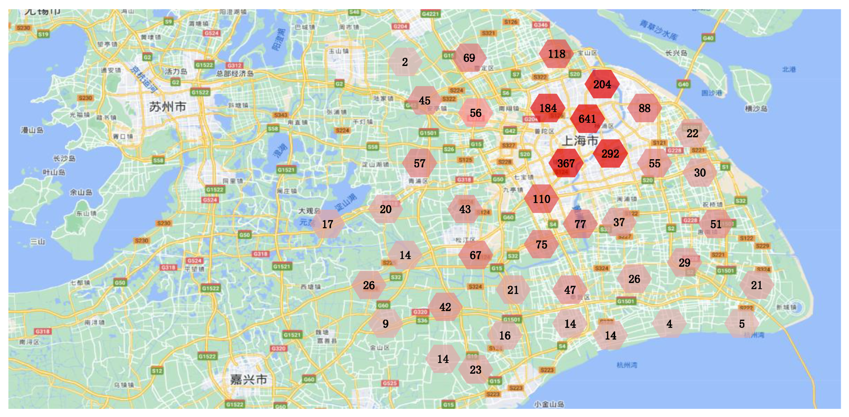
We used the Shanghai Telecom base station dataset [38] to obtain real BS information and the data of UDs accessing the Internet through BSs. The Shanghai Telecom base station dataset contains accurate location information of 3233 BSs and detailed information of mobile UDs accessing the Internet through these BSs [39]. Specifically, the dataset includes over 72 million traffic access records of 7481 UDs accessing the Internet through 3233 BSs. Each record contains start and end time when a mobile UD accesses the Internet through a certain BS. We randomly selected a period and counted the duration of each UD accessing the Internet through each BS in that period, as well as the total duration of each UD accessing the Internet through all BSs in that period. We analyzed each record and extracted UD information (i.e., start and end time when the UD accessed the Internet through a BS) and BS information (i.e., latitude and longitude of the BS). Figure 6 shows the distribution of 3233 BSs in the Shanghai base station dataset. Each region in Figure 6 is represented by a hexagon, and the number on each hexagon represents the number of BSs in that region.

By analyzing the association between each UD and each BS, we can calculate the probability of each UD appearing within the coverage range of each BS during that period (i.e., ${\Phi }_q=\left\{p_{qv}|v\in V\right\}$, where $p_{qv}$ is shown in (77)).

$$p_{qv}=\frac{\mathrm{Duration} \mathrm{of} \mathrm{UD} q’\mathrm{s} \mathrm{association} \mathrm{with} \mathrm{BS} v \mathrm{during} \mathrm{that} \mathrm{period}}{ \mathrm{Total} \mathrm{duration} \mathrm{of} \mathrm{UD} q’\mathrm{s} \mathrm{association} \mathrm{with} \mathrm{all} \mathrm{BSs} \mathrm{in} \mathrm{that} \mathrm{period}}$$

(77)

We assume that each cloudlet is deployed adjacent to a BS, and the probability of generating a direct link between any pair of BSs follows an exponential model, i.e., the probability of generating a direct link between any two BSs decreases exponentially with the increase in their Euclidean distance, and the probability function is $\beta \left(\mathrm{u},v\right)=a*exp\left(-{\tilde{d}}_{ij}/\left(\sqrt{2}L-{\tilde{d}}_{ij}\right)\right)$, where $L$ represents the maximum Euclidean distance between any two BSs in a network, ${\tilde{d}}_{ij}$ represents the Euclidean distance between $v_i$ and $v_j$ that can be calculated based on the geographical location (longitude and latitude) of BSs, and $a$ is a positive decimal number set to adjust the number of links between BSs (we set it as 0.006). The larger the value of a, the greater the probability of generating direct links between any two base stations, and the greater the number of links between base stations. The smaller the value of a, the smaller the probability of generating direct links between any two base stations, and the smaller the number of links between base stations.

5.2. Memory Page Simulation

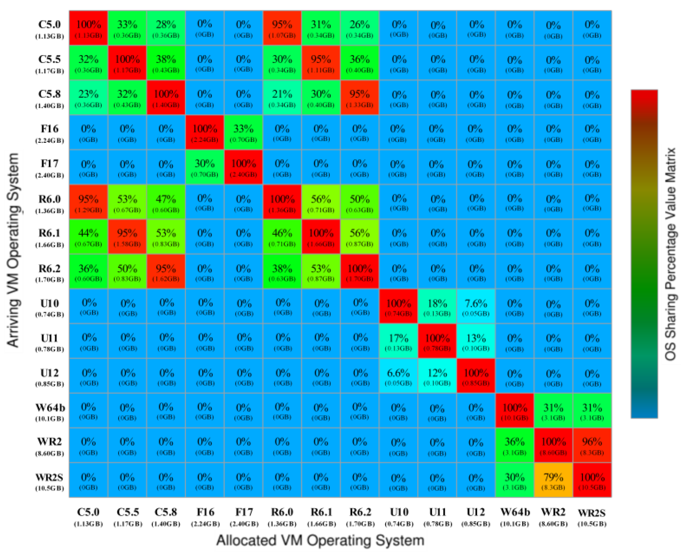
When maximizing memory sharing between VMs, it is necessary to identify the applications and operating systems running on the VMs to be instantiated, which cannot be obtained from ClusterData. Although each task event operates in its own container [25], we consider each task event as a VM instance running a different operating system. In our experiments, we considered the percentage of page content similarity between different operating systems reported by Bazarbayev et al. [40], as shown in Figure 7. We considered a fixed memory-sharing percentage for any combination of two operating systems in experiments. Each entry in Figure 7 represents the percentage of memory sharing between a pair of operating systems, which is defined as the proportion of memory used by the operating system of an already instantiated VM that can be shared with the operating system of a newly arrived VM.

In our experiments, we assume that the operating system of each VM is randomly selected from 14 versions of 5 types of operating systems, including CentOS Server x86_64 (C5.0, C5.5, C5.8), Fedora x86_64 (F16, F17), Red Hat Enterprise Linux x86_64 (R6.0, R6.1, R6.2), Ubuntu Server i386 (U10, U11, U12), and Windows Server (W64b, WR2, WR2S). For each version of operating system, we associate a binary array that specifies the required memory pages, based on the memory-sharing ratio between different operating systems. If a page is requested by an operating system, the corresponding entry for that page in the binary array of that system is set to 1; otherwise, it is set to 0.

5.3. Experimental Method

All experiments were conducted on a PC (Windows 10) with the following specifications: AMD Ryzen 5 4600H with Radeon Graphics 3.00 GHz and 16.0 GB RAM.

We conducted experiments in three parts; in each part, we randomly selected a portion of UDs from the Shanghai Telecom base station dataset to form the set of UDs used in experiments and randomly selected a portion of BSs as the deployment location of cloudlets. We use UP to represent the ratio of the selected UDs to the total number of UDs, and we use CP to represent the ratio of the selected BSs to the total number of BSs; CP can also be viewed as the ratio of the number of deployed cloudlets to the total number of BSs.

The first part uses the weighted sum method to verify that maximizing memory sharing between VMs and minimizing average communication distance between VMs and UDs cannot be achieved simultaneously in experimental scenarios with different CP and UP, and the two objectives conflict with each other. In the second part, we designed three experimental scenarios based on three different CPs to compare results of the iterative heuristic algorithm and the weighted sum method. In each scenario, the links between BSs are fixed, the parameters of cloudlets are also fixed, and we set up six different UPs to determine the number of VMs. Meanwhile, we compared the computation time of the iterative heuristic algorithm and the weighted sum method. In the third part, we designed three experimental scenarios based on three different CPs to compare results of the iterative heuristic algorithm and other benchmark algorithms. In each scenario, the links between BSs are fixed, the parameters of cloudlets are also fixed, and we set up five different UPs for validation.

In order to facilitate the superiority of the iterative heuristic algorithm (ε-CBIHA), we selected some benchmark VM instantiation methods for comparison: the first is the memory sharing greedy heuristic algorithm (RSGA), which first sorts VMs into groups based on their potential for sharing memory and then greedily instantiates VM groups in cloudlets. The second is the average communication distance greedy heuristic algorithm (ADGA), which first sorts VMs in ascending order based on the sum of communication distances between each VM and all BSs and then determines the instantiation location for each VM in turn. The third is a random allocation algorithm (Random), used to select a random cloudlet to instantiate VMs. The fourth is the weighted sum method based on the ILP method (IBWSA), which combines the two objective functions into a single-objective function through weighted summation and solves it based on an ILP solver.

5.4. Experimental Results and Analysis

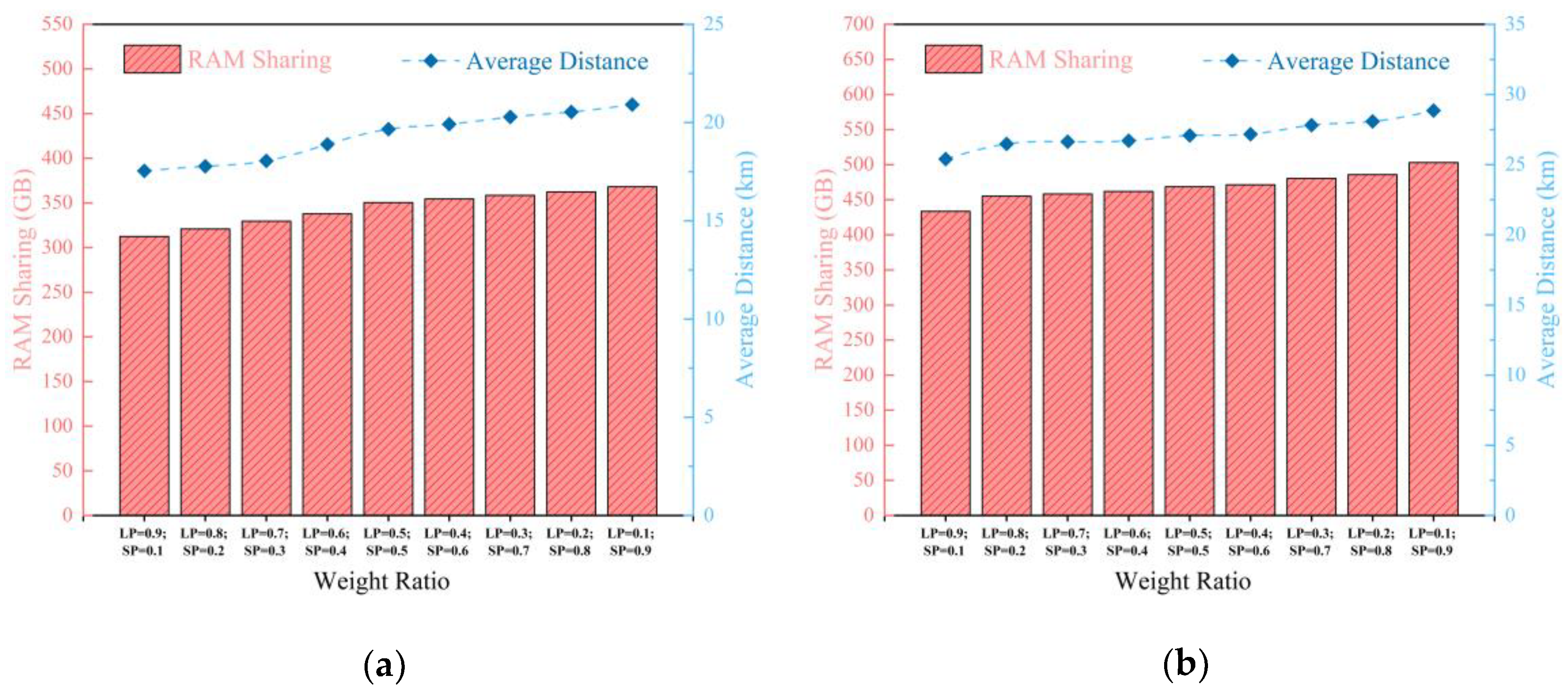
In the first part, we selected two pairs of UP and CP to construct two experimental scenarios, namely CP = 0.0138, UP = 0.012, and CP = 0.0104, UP = 0.0135. We set up nine sets of comparative experiments by changing the weights of two objectives. We use SP and LP to represent the weights of memory sharing among VMs and average communication distance between VMs and UDs, respectively. We initialize SP to 0.1 and increase it to 0.9 in steps of 0.1, while initializing LP to 0.9 and decreasing it to 0.1 in steps of 0.1.

Figure 8a,b respectively show the experimental results obtained by adjusting SP and LP in experimental scenarios with CP = 0.0138 and UP = 0.012 as well as CP = 0.0104 and UP = 0.0135. We can see that the trends of these two goals are opposite. As the SP increases, the value of memory sharing between VMs increases correspondingly, while the decrease in LP leads to an increase in average communication distance between VMs and UDs. Therefore, it is not possible to simultaneously achieve these two goals in experimental scenarios with different CPs and UPs.

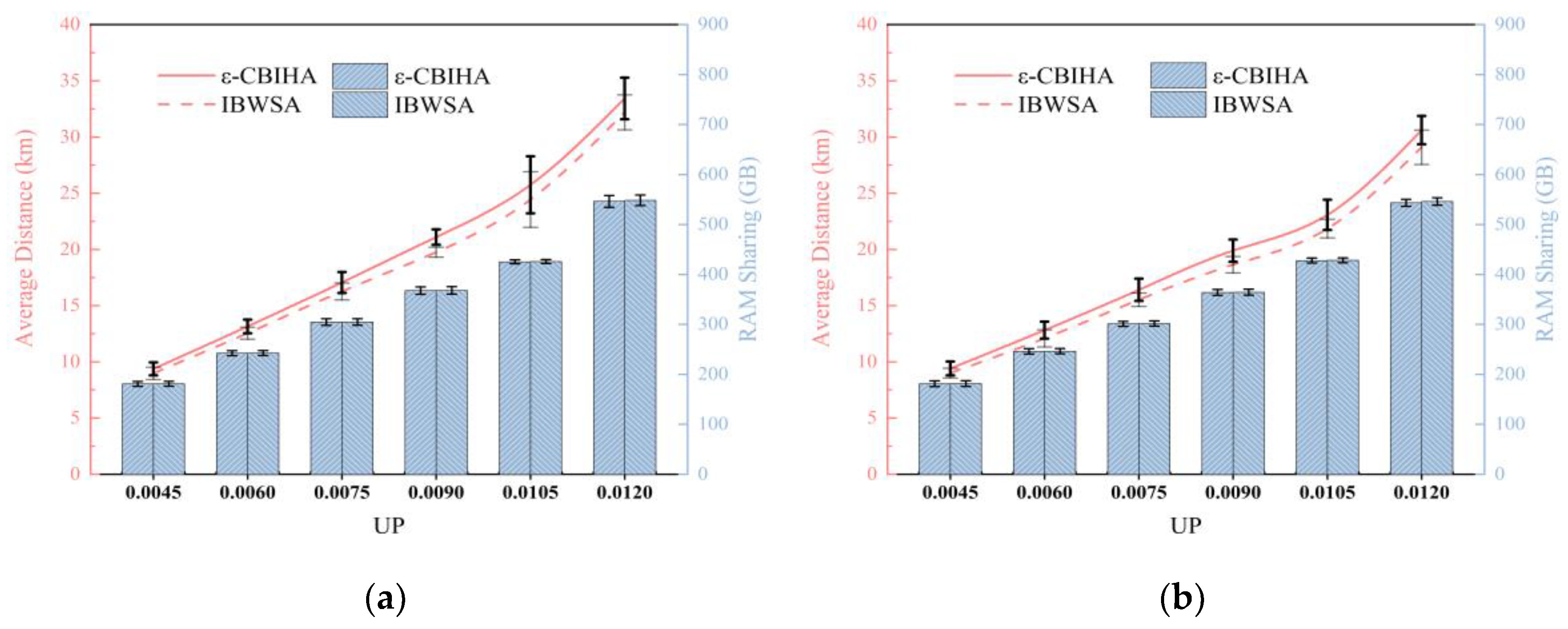
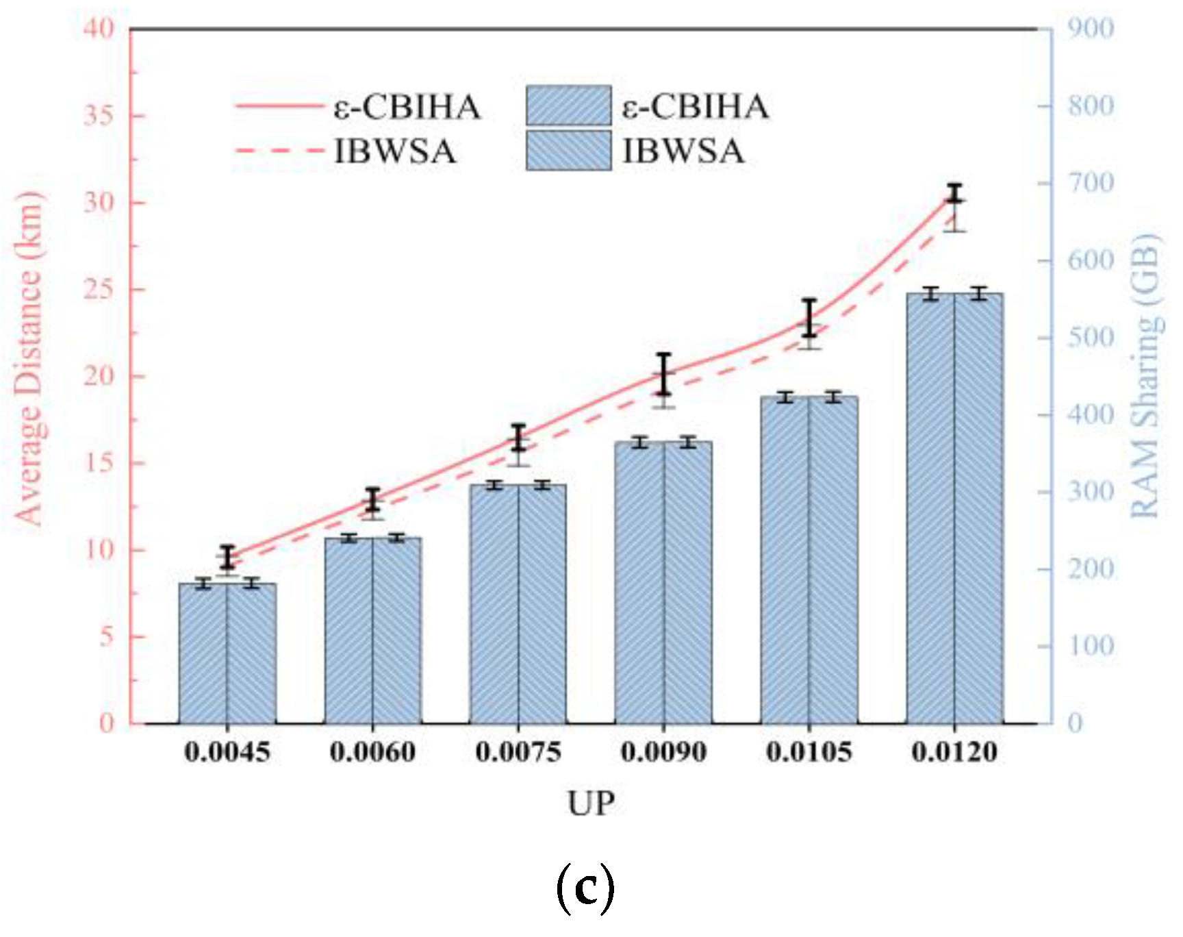
In the second part, we designed three experimental scenarios based on three different CPs, i.e., CP = 0.0104, CP = 0.0138, and CP = 0.0172, and we set six different UPs to determine the number of VMs, i.e., UP = {0.0045, 0.006, 0.0075, 0.009, 0.0105, 0.012}, and then, the mean and standard deviation of experimental results were calculated by selecting VMs with different parameters for multiple experiments. Figure 9 shows the results of IBWSA and ε-CBIHA for six different UPs in three experimental scenarios with CP = 0.0104, CP = 0.0138, and CP = 0.0172, respectively.

We can see that the results obtained with IBWSA and ε-CBIHA are almost equal in terms of memory sharing, and the standard deviations of the results obtained with both are also almost equal. In terms of average communication distance, the results obtained with ε-CBIHA are slightly worse than results obtained with IBWSA, and we observe that in the experimental scenario with CP = 0.0104, the standard deviation of results obtained with IBWSA and ε-CBIHA when UP ≥ 0.0105 is larger than that obtained when UP < 0.0105. We speculate that when CP = 0.0104 and UP = 0.009, all VMs can be instantiated in cloudlets, so the results obtained with IBWSA and ε-CBIHA are relatively stable. However, when CP = 0.0104 and UP = 0.0105, the number of VMs increases so that cloudlets cannot host all the VMs, and some VMs can only be instantiated in public data centers, resulting in large fluctuations in the standard deviation of the results obtained with IBWSA and ε-CBIHA.

We compare the computation time of IBWSA and ε-CBIHA in the following. We randomly select nine different CP and UP pairs to form experimental scenarios and run IBWSA and ε-CBIHA 10 times in each scenario. We calculate the average computation time of the two algorithms, as shown in

Table 5. Calculation time of IBWSA and ε-CBIHA.

Group	Calculation Time of ε-CBIHA	Calculation Time of IBWSA	Ratio of Calculation Time
1	282.2	287.6	98.12%
2	798.0	1115.4	71.54%
3	2820.5	5105.8	55.23%
4	1089.0	1098.7	99.11%
5	3548.6	5217.0	68.01%
6	10,333.2	17,632.7	58.60%
7	1485.7	2041.0	72.79%
8	3790.2	7216.6	52.51%
9	11,564.6	20,218.9	57.19%

. The results show that in all nine experimental scenarios, the computation time of ε-CBIHA is smaller than that of IBWSA, and the difference between the two becomes larger as the size of the scenario increases. The average computation time of ε-CBIHA is only 70.34% of that of IBWSA, and in the best, the computation time of ε-CBIHA is 52.51% of that of IBWSA. Therefore, the iterative heuristic algorithm proposed in this paper can indeed speed up the solution process.

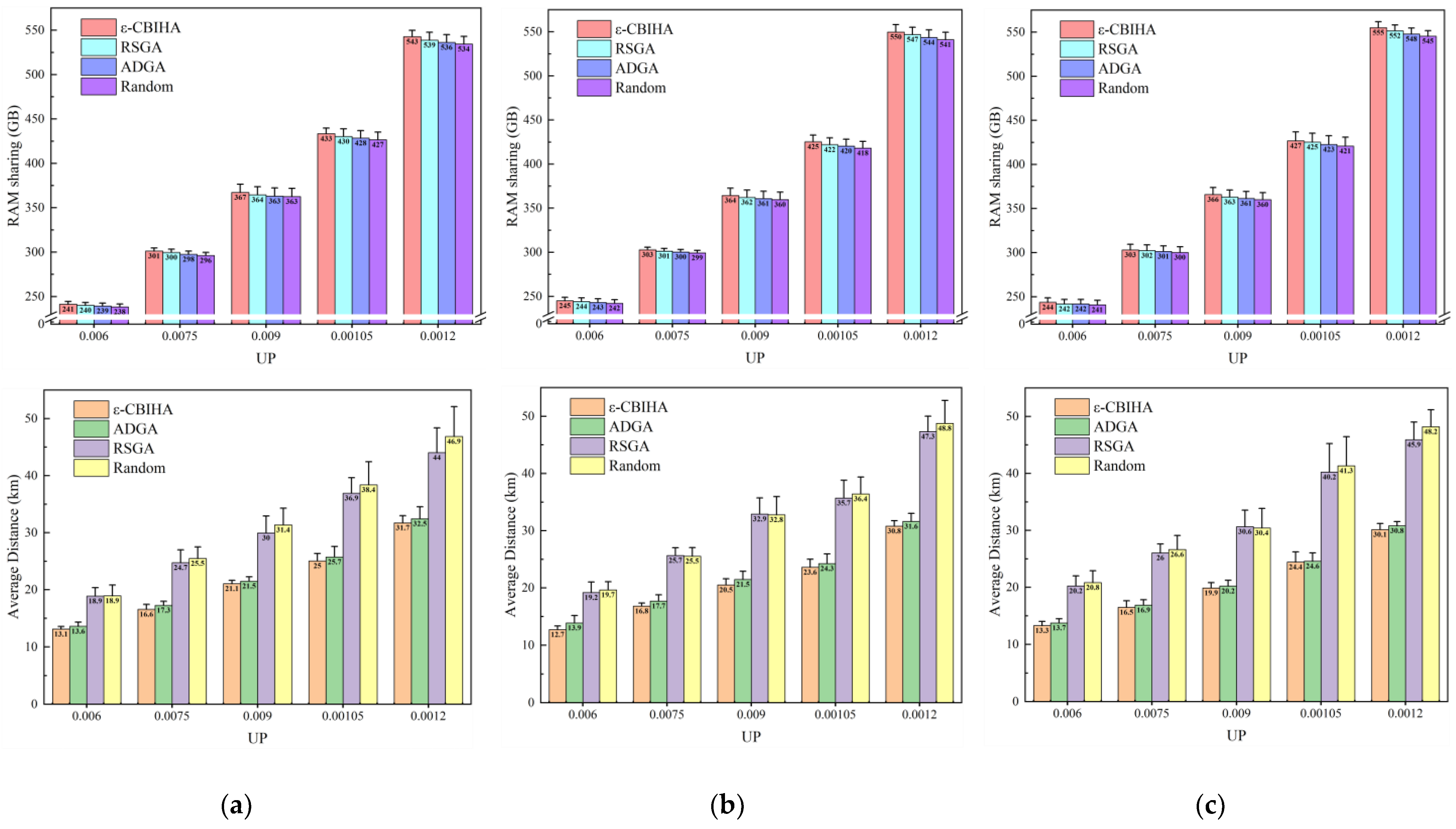
In the third part, we compare the results obtained with ε-CBIHA with those obtained using other baseline algorithms. Figure 10 shows the results of ε-CBIHA and three baseline algorithms under different CPs and UPs. The values of CP are 0.0104, 0.0172, and 0.024, while the values of UP are 0.006, 0.0075, 0.009, 0.0105, and 0.012. In these three figures, we can observe that ε-CBIHA has better performance than other algorithms. In all cases, the value of memory sharing among VMs obtained with ε-CBIHA is greater than those obtained using other algorithms, and the value of average communication distance between VMs and UDs obtained with ε-CBIHA is also smaller than those obtained using other algorithms.

In each figure, we can see that in terms of memory sharing among VMs, the results obtained with ε-CBIHA are the best, followed by RSGA and ADGA, and finally the Random. The results obtained with ε-CBIHA are about 3.6% higher than other baseline algorithms overall. In terms of average communication distance between VMs and UDs, the results obtained with ε-CBIHA are the best, followed by ADGA and RSGA, and finally the Random method. The results obtained with ε-CBIHA are about 22.7% lower than other baseline algorithms overall. ADGA is better than RSGA in minimizing average communication distance between VMs and UDs, while RSGA is better than ADGA in maximizing memory sharing among VMs. The Random may not be able to instantiate VMs with more identical memory pages in the same cloudlet or instantiate VMs in cloudlets with a larger average communication distance from their UDs, so the results obtained using this method are the worst in both aspects.

Meanwhile, we observed that with the continuous increase in CP, the results obtained with ε-CBIHA under the same UP showed an overall upward trend in memory sharing among VMs and an overall downward trend in average communication distance between VMs and UDs. We speculate that the continuous increase in CP leads to more optional cloudlets available when instantiating VMs, which is conducive to further increasing the probability of instantiating VMs in cloudlets with smaller average communication distances to UDs or increasing the probability of aggregating VMs with more identical memory pages in the same cloudlet.

6. Conclusions and Future Work

In this paper, we have addressed the problem of virtual machine instantiation with the joint optimization of memory sharing and communication distance in cloudlet networks, which is a bi-objective optimization problem. The problem has been formulated as VM memory sharing maximization and average communication distance minimization problem to find the solution for virtual machine instantiation. Then, we designed an iterative heuristic algorithm based on the ε-constraint method, which decomposes the bi-objective optimization problem into multiple single-objective optimization subproblems, and iteratively obtains the subproblems’ optimal solutions. Finally, extensive experiments have been conducted on actual datasets to validate the feasibility and effectiveness of our algorithm.

Regarding the problem of virtual machine instantiation with the joint optimization of memory sharing and communication distance in cloudlet networks, the algorithm proposed in this article is only suitable for obtaining accurate solutions in small-scale cloudlet networks. However, in large-scale cloudlet networks, the algorithm proposed in this paper cannot obtain representative Pareto solutions within an acceptable time. When setting up the experimental environment, we assume that each cloudlet has only one server without considering the heterogeneity of cloudlets, which is different from real cloudlet networks. At the same time, when considering memory sharing between virtual machines, we only consider the memory pages related to operating systems, without considering the dynamic shareability of memory pages within virtual machines. In future work, we will consider how to achieve more memory sharing between virtual machines with different distributed locations based on application categories in heterogeneous cloudlet networks.

References

- Jararweh, Y.; Tawalbeh, L.; Ababneh, F.; Dosari, F. Resource Efficient Mobile Computing Using Cloudlet Infrastructure. In Proceedings of the 2013 IEEE 9th International Conference on Mobile Ad-hoc and Sensor Networks, Dalian, China, 11–13 December 2013; pp. 373–377. [Google Scholar]
- Uma, D.; Udhayakumar, S.; Tamilselvan, L.; Silviya, J. Client Aware Scalable Cloudlet to Augment Edge Computing with Mobile Cloud Migration Service. Int. J. Interact. Mob. Technol. IJIM 2020, 14, 165. [Google Scholar] [CrossRef]
- Vhora, F.; Gandhi, J. A Comprehensive Survey on Mobile Edge Computing: Challenges, Tools, Applications. In Proceedings of the 2020 Fourth International Conference on Computing Methodologies and Communication (ICCMC), Erode, India, 11–13 March 2020; pp. 49–55. [Google Scholar]
- Satyanarayanan, M.; Bahl, P.; Caceres, R.; Davies, N. The Case for VM-Based Cloudlets in Mobile Computing. IEEE Pervasive Comput. 2009, 8, 14–23. [Google Scholar] [CrossRef]
- Borcea, C.; Ding, X.; Gehani, N.; Curtmola, R.; Khan, M.A.; Debnath, H. Avatar: Mobile Distributed Computing in the Cloud. In Proceedings of the 2015 3rd IEEE International Conference on Mobile Cloud Computing, Services, and Engineering, San Francisco, CA, USA, 30 March–3 April 2015; pp. 151–156. [Google Scholar]
- Shaukat, U.; Ahmed, E.; Anwar, Z.; Xia, F. Cloudlet Deployment in Local Wireless Networks: Motivation, Architectures, Applications, and Open Challenges. J. Netw. Comput. Appl. 2016, 62, 18–40. [Google Scholar] [CrossRef]
- Jin, X.; Li, L.E.; Vanbever, L.; Rexford, J. SoftCell: Scalable and Flexible Cellular Core Network Architecture. In Proceedings of the Ninth ACM Conference on Emerging Networking Experiments and Technologies, Santa Barbara, CA, USA, 9–13 December 2013; Association for Computing Machinery: New York, NY, USA, 2013; pp. 163–174. [Google Scholar]
- Sun, X.; Ansari, N. Adaptive Avatar Handoff in the Cloudlet Network. IEEE Trans. Cloud Comput. 2019, 7, 664–676. [Google Scholar] [CrossRef]
- Haimes, Y. On a Bicriterion Formulation of the Problems of Integrated System Identification and System Optimization. IEEE Trans. Syst. Man Cybern. 1971, SMC-1, 296–297. [Google Scholar] [CrossRef]
- Bugnion, E.; Devine, S.; Govil, K.; Rosenblum, M. Disco: Running Commodity Operating Systems on Scalable Multiprocessors. ACM Trans. Comput. Syst. 1997, 15, 412–447. [Google Scholar] [CrossRef]
- Waldspurger, C.A. Memory Resource Management in VMware ESX Server. ACM SIGOPS Oper. Syst. Rev. 2003, 36, 181–194. [Google Scholar] [CrossRef]
- Pan, Y.-S.; Chiang, J.-H.; Li, H.-L.; Tsao, P.-J.; Lin, M.-F.; Chiueh, T. Hypervisor Support for Efficient Memory De-Duplication. In Proceedings of the 2011 IEEE 17th International Conference on Parallel and Distributed Systems, Tainan, Taiwan, 7–9 December 2011; pp. 33–39. [Google Scholar]
- Ji, H.; Mansi, M.; Sun, Y.; Yuan, Y.; Huang, J.; Kuper, R.; Swift, M.M.; Kim, N.S. STYX: Exploiting SmartNIC Capability to Reduce Datacenter Memory Tax. In Proceedings of the 2023 USENIX Annual Technical Conference, Boston, MA, USA, 10–12 July 2023; pp. 619–633. [Google Scholar]
- Ge, Y.; Tian, Y.-C.; Yu, Z.-G.; Zhang, W. Memory Sharing for Handling Memory Overload on Physical Machines in Cloud Data Centers. J. Cloud Comput. 2023, 12, 27. [Google Scholar] [CrossRef]
- Wood, T.; Tarasuk-Levin, G.; Shenoy, P.; Desnoyers, P.; Cecchet, E.; Corner, M.D. Memory Buddies: Exploiting Page Sharing for Smart Colocation in Virtualized Data Centers. ACM SIGOPS Oper. Syst. Rev. 2009, 43, 27–36. [Google Scholar] [CrossRef]
- He, Q.; Li, Z.; Chen, C.; Feng, H. Research on Global BloomFilter-Based Data Routing Strategy of Deduplication in Cloud Environment. IETE J. Res. 2023, 1–11. [Google Scholar] [CrossRef]
- Rampersaud, S.; Grosu, D. A Sharing-Aware Greedy Algorithm for Virtual Machine Maximization. In Proceedings of the 2014 IEEE 13th International Symposium on Network Computing and Applications, Cambridge, MA, USA, 21–23 August 2014; pp. 113–120. [Google Scholar]
- Rampersaud, S.; Grosu, D. An Approximation Algorithm for Sharing-Aware Virtual Machine Revenue Maximization. IEEE Trans. Serv. Comput. 2021, 14, 1–15. [Google Scholar] [CrossRef]
- Sartakov, V.A.; Vilanova, L.; Geden, M.; Eyers, D.; Shinagawa, T.; Pietzuch, P. ORC: Increasing Cloud Memory Density via Object Reuse with Capabilities. In Proceedings of the 17th USENIX Symposium on Operating Systems Design and Implementation, Boston, MA, USA, 10–12 July 2023; pp. 573–587. [Google Scholar]
- Jagadeeswari, N.; Mohanraj, V.; Suresh, Y.; Senthilkumar, J. Optimization of Virtual Machines Performance Using Fuzzy Hashing and Genetic Algorithm-Based Memory Deduplication of Static Pages. Automatika 2023, 64, 868–877. [Google Scholar] [CrossRef]
- Qiu, W. Memory Deduplication on Serverless Systems. Master’s Thesis, ETH Zürich, Zürich, Switzerland, 2015. [Google Scholar]
- Jagadeeswari, N.; Mohan Raj, V. Homogeneous Batch Memory Deduplication Using Clustering of Virtual Machines. Comput. Syst. Sci. Eng. 2023, 44, 929–943. [Google Scholar] [CrossRef]
- Du, C.; Wu, S.; Wu, J.; Mao, B.; Wang, S. ESD: An ECC-Assisted and Selective Deduplication for Encrypted Non-Volatile Main Memory. In Proceedings of the 2023 IEEE International Symposium on High-Performance Computer Architecture (HPCA), Montreal, QC, Canada, 25 February–1 March 2023; pp. 977–990. [Google Scholar]
- Sun, X.; Ansari, N. Latency Aware Workload Offloading in the Cloudlet Network. IEEE Commun. Lett. 2017, 21, 1481–1484. [Google Scholar] [CrossRef]
- Genez, T.A.L.; Tso, F.P.; Cui, L. Latency-Aware Joint Virtual Machine and Policy Consolidation for Mobile Edge Computing. In Proceedings of the 2018 15th IEEE Annual Consumer Communications & Networking Conference (CCNC), Las Vegas, NV, USA, 12–15 January 2018; pp. 1–6. [Google Scholar]
- Liu, G.; Wang, J.; Tian, Y.; Yang, Z.; Wu, Z. Mobility-Aware Dynamic Service Placement for Edge Computing. EAI Endorsed Trans. Internet Things 2019, 5, e2. [Google Scholar] [CrossRef]
- Sun, X.; Ansari, N. Green Cloudlet Network: A Distributed Green Mobile Cloud Network. IEEE Netw. 2017, 31, 64–70. [Google Scholar] [CrossRef]
- Landa, R.; Araújo, J.T.; Clegg, R.G.; Mykoniati, E.; Griffin, D.; Rio, M. The Large-Scale Geography of Internet Round Trip Times. In Proceedings of the 2013 IFIP Networking Conference, Brooklyn, NY, USA, 22–24 May 2013; pp. 1–9. [Google Scholar]
- van Adrichem, N.L.M.; Doerr, C.; Kuipers, F.A. OpenNetMon: Network Monitoring in OpenFlow Software-Defined Networks. In Proceedings of the 2014 IEEE Network Operations and Management Symposium (NOMS), Krakow, Poland, 5–9 May 2014; pp. 1–8. [Google Scholar]
- Yu, C.; Lumezanu, C.; Sharma, A.; Xu, Q.; Jiang, G.; Madhyastha, H.V. Software-Defined Latency Monitoring in Data Center Networks. In Passive and Active Measurement; Mirkovic, J., Liu, Y., Eds.; Springer International Publishing: Cham, Switzerland, 2015; pp. 360–372. [Google Scholar]
- Wu, P.; Che, A.; Chu, F.; Zhou, M. An Improved Exact ε-Constraint and Cut-and-Solve Combined Method for Biobjective Robust Lane Reservation. IEEE Trans. Intell. Transp. Syst. 2015, 16, 1479–1492. [Google Scholar] [CrossRef]
- Esmaili, M.; Amjady, N.; Shayanfar, H.A. Multi-Objective Congestion Management by Modified Augmented ε-Constraint Method. Appl. Energy 2011, 88, 755–766. [Google Scholar] [CrossRef]
- Reiss, C.; Wilkes, J.; Hellerstein, J.L. Google Cluster-Usage Traces: Format+ Schema; White Paper; Google Inc.: Mountain View, CA, USA, 2011; pp. 1–14. [Google Scholar]
- Google Cloud Storage. Available online: https://cloud.google.com/storage/docs/overview (accessed on 7 January 2023).
- Google Compute Engine Pricing. Available online: https://cloud.google.com/compute/pricing (accessed on 7 January 2023).
- Google Compute Engine Disks. Available online: https://cloud.google.com/compute/docs/disks (accessed on 9 January 2023).
- Second Quarter 2015 SPECvirt_sc2013 Results. Available online: https://www.spec.org/virt_sc2013/ (accessed on 14 January 2023).
- The Distribution of 3233 Base Stations. Available online: http://www.sguangwang.com/dataset/telecom.zip (accessed on 12 January 2023).
- Wang, S.; Zhao, Y.; Xu, J.; Yuan, J.; Hsu, C.-H. Edge Server Placement in Mobile Edge Computing. J. Parallel Distrib. Comput. 2019, 127, 160–168. [Google Scholar] [CrossRef]
- Bazarbayev, S.; Hiltunen, M.; Joshi, K.; Sanders, W.H.; Schlichting, R. Content-Based Scheduling of Virtual Machines (VMs) in the Cloud. In Proceedings of the 2013 IEEE 33rd International Conference on Distributed Computing Systems, Philadelphia, PA, USA, 8–11 July 2013; pp. 93–101. [Google Scholar]
Figure 1.
Architecture of cloudlet networks. (Remote cloud data centers, software-defined networks, and wireless local area networks form the three-layer structure of cloudlet network.)
Figure 2.
Memory pages required for instantiating VMs. (The shaded boxes in each row correspond to the memory pages requested by each VM. The thick vertical lines connecting shaded boxes indicate the same pages between VMs.)
Figure 3.
Diagram of VM instantiation process. (When , four VMs, and , need to be instantiated in two cloudlets, and ; has already been instantiated in , and its memory pages have been hosted in the memory space of . In the first iteration, is greater than the other , so when , should be instantiated in . Then, we compare the memory pages of with those hosted in and add different memory pages to ’s memory space. Next, we add to , update , and recalculate for remaining VMs with corresponding cloudlets. Repeat the above process until and are all allocated and instantiated in and .)
Figure 4.
Diagram of VM instantiation location. (Value of is not the only determining factor affecting instantiation of VMs, and average communication distance will also affect instantiation of VMs.)
Figure 5.
Illustration of ideal point, nadir point, and Pareto front.
Figure 6.
Distribution of Shanghai Telecom base stations. (The above figure mainly shows the distribution of streets and urban areas around Shanghai. The text in the figure indicates the urban area of Shanghai and its surrounding towns. Each region is represented by a hexagon, and the number on each hexagon represents the number of BSs in that region.)
Figure 7.
Memory sharing between operating systems. (The percentage of memory sharing between a pair of operating systems, which is defined as the proportion of memory used by the operating system of an already instantiated VM that can be shared with the operating system of a newly arrived VM.)
Figure 8.
(a) Results for IBWSA with different weights in CP = 0.0138 and UP = 0.012 scenario; (b) results for IBWSA with different weights in CP = 0.0104 and UP = 0.0135 scenario. (As the SP increases, the value of memory sharing between VMs increases correspondingly, while the decrease in LP leads to an increase in average communication distance between VMs and UDs.)
Figure 9.
(a) Results for IBWSA and ε-CBIHA with different UPs in CP = 0.0104 scenario; (b) results for IBWSA and ε-CBIHA with different UPs in CP = 0.0138 scenario; and (c) results for IBWSA and ε-CBIHA with different UPs in CP = 0.0172 scenario. (The results obtained with IBWSA and ε-CBIHA are almost equal in terms of memory sharing, and the standard deviations of the results obtained with both are also almost equal. In terms of average communication distance, the results obtained with ε-CBIHA are slightly worse than results obtained with IBWSA.)
Figure 10.
(a) Results of ε-CBIHA and benchmark algorithms in CP=0.0104 scenario; (b) results of ε-CBIHA and benchmark algorithms in CP = 0.0172 scenario; (c) results of ε-CBIHA and benchmark algorithms in CP = 0.024 scenario. (In terms of memory sharing among VMs, the results obtained with ε-CBIHA are the best, followed by RSGA and ADGA, and finally the Random. In terms of average communication distance between VMs and UDs, the results obtained with ε-CBIHA are the best, followed by ADGA and RSGA, and finally the Random method.)