
A Risk Curtailment Strategy for Solar PV-Battery Integrated Competitive Power System


1
Department of Electrical Engineering, Mizoram University, Aizawl 796004, Mizoram, India
2
Department of Electrical & Electronics Engineering, Velagapudi Ramakrishna Siddhartha Engineering College, Vijayawada 520007, Andhra Pradesh, India
3
Fukushima Renewable Energy Institute, AIST (FREA), Koriyama 963-0298, Japan
*
Author to whom correspondence should be addressed.
Electronics 2022, 11(8), 1251; https://doi.org/10.3390/electronics11081251
Submission received: 28 February 2022
/
Revised: 31 March 2022
/
Accepted: 11 April 2022
/
Published: 15 April 2022
(This article belongs to the Special Issue Feature Papers in Industrial Electronics)
Abstract
:Power system networks are becoming more complex and decentralized with the foreword of deregulation in the global power sector. In this scenario, an independent system operator (ISO) is responsible for determining the appropriate actions to deliver stable and quality power to the customers connected to the network at the lowest cost without violating the system security limits. Violations of any security limit may result in system risk. The unstable and non-reliable system always has some drawbacks and is not desirable from the consumer’s point of view. A deregulated power market always keeps the consumer on the advantage side by giving stable, reliable, and less costly power. By using risk assessment tools, we identify the fault conditions and we try to minimize the risk by various uses of sequential programming methods. In this paper, a novel power system risk analysis and congestion management approach are introduced with considering meta-heuristic algorithms i.e., Slime Mould Algorithm (SMA) and Artificial Bee Colony Algorithm (ABC) in renewable energy integrated electricity market. The proposed power system risk analysis is constructed with the help of two risk valuation tools named Conditional-Value-at-risk (CVaR) and Value-at-risk (VaR). The higher negative value of VaR and CVaR represents the higher risk system and lower negative value or towards a positive value of VaR and CVaR denotes the less risk or stable system. The projected method has been experienced on the IEEE 14-bus test system and IEEE 30-bus test system to examine the usefulness of the meta-heuristic algorithm in system risk analysis under the deregulated environment. The importance of renewable energy integration in system risk curtailment has also been depicted in this work: basically, to measure the system’s risk, hence enhancing the system’s reliability and societal welfare. As a result, it will benefit both supply and demand-side participants.
1. Introduction
The reformation of the electrical system creates a huge change in the area of competitiveness among all the market participants i.e., Generation companies (GENCOs), Transmission Companies (TRANSCOs), Distribution Companies (DISCOs), and retailers. This market environment generates the field where the customers are more profitable than the earlier stage [1]. Due to the need for more energy to the customers for their use of high-end technology, the energy requirement is rapidly increasing. The setup of a new power generation station is required to achieve this continuously increasing demand. However, this is very difficult due to the social, economic, political, and environmental barriers [2]. Considering the existing power delivery channel, power generating stations cannot transmit extra power. If this is tried from GENCOs side then system risk may occur like transmission congestion, voltage fluctuation, grid failure, etc.
Due to the decentralized concept of the deregulated power system, renewable sources and energy storage system incorporation in the modern power system is very easy. Renewable energy plays a significant role to minimize the variance between power generation and demand. The combined operation of conventional and renewable energy sources can minimize the system risk by reducing the mismatch between power generation and demand. The restrictions in the construction of new transmission lines force the companies to develop new technologies for transmitting power through the existing lines [3,4]. However, there is a limitation in power flow through the present transmission channel due to the thermal limits of the transmission lines. If more power is flowing through the transmission lines, the electrical power system becomes overloaded, and then system congestion is generated. In the deregulated environment, overloading of the power system may avoid the execution of new technologies, which may affect the total use of the system. For that reason, the maximization of profit may be hampered [5]. In recent years, very limited technologies have developed to curtail the system risk in the domain of renewable energy and the competitive power market.
Due to the competitive nature of the electric market, the power prices are likely to become low which pays back the consumers. The main purpose of the deregulated power market is to promote competition among the GENCOs and the Customers to perk up the service quality and continuity of supply, to uphold the economy and overall efficiency of the power system. Conservative energy sources are degraded very rapidly which forces transition to renewable energy sources, which also experience degradation but to a lesser degree [6]. As per the review, India will generate 40% of total power by renewable energy sources by 2030, among which 100 GW from solar, 60 GW from wind, 10 GW from bio-power, and 5 GW from small hydro power [7]. Renewable energy sources not only meet the fast-growing electricity demand but also reduce the system economic risk in the competitive power market.
Under the uncertainty of risk measurement, optimization plays a crucial role, especially in conjunction with the losses to the system. Some efforts have been made by researchers in recent years to solve several problems related to risk assessment. The most popular parameter for measuring system risk is value-at-risk (VaR). However, if losses are not distributed uniformly then it is very difficult to calculate. VaR is also not consistent. The circumstances of the loss are not considered in the calculation of VaR. An alternative measurement strategy that meets the condition of loss is called Conditional-value-at-risk (CVaR). CVaR has many advanced features. It maintains uniformity with VaR in terms of the same results in limited settings.
To calculate the system risk in a power system, the most effective risk assessment tools are VaR and CVaR. These parameters can assess the stability and condition of power flow in a system. The risk that appeared in the power system is calculated and will be minimized by the use of renewable energy sources [8]. Rockafellar et al. [9] show the superiority of CVaR over the VaR in power system risk assessment in the presence of stability factors. A power system unit is not only trying to improve the system losses and risk but also attempting to maximize social welfare [10]. Many researchers have done their work in the field of system risk [11,12]. Li et al. [13] propose a methodology for assessing the system safety and mitigation of system risk of a hydroelectric system. Yun et al. [14] depict a risk valuation method for assessing the effect of voltage sag in a power network. A hybrid method is advised in [15] to reduce the weather-based system risk in the presence of wind power in a competitive power market. Paper [16] portrays an approach for handling the several climates that produced risks in a Canadian power system. Shiwen et al. [17] discussed the benefit and drawbacks of several risk valuation methods of a power network. A risk assessment methodology of the nuclear power plant has been deliberated in [18] in the presence of components aging. A probabilistic approach has been studied in [19] for analyzing the power system blackout and its risk in the system. Salman et al. [20] present probabilistic content for risk evaluation in a power system with seismic conditions. Ref. [21] presents load flow studies based on the probability for evaluating the system risk of a solar included power system.
Some research has also been studied earlier by several researchers regarding congestion management. Ghazvini et al. [22] present the market-based method to improve the congestion of the distribution network by the home energy management system (HEMS). A joint constant pricing method has been discussed in [23] for improving the system congestion in a distributed network. Wang et al. [24] proposed a risk assessment technique of an electrical power system with the influence of an electric transport system. When a large number of electrified vehicles start working on a single power network frame, how congestion may occur is described in this work. The importance of renewable energy from the reliability point of view over generating systems is discussed in [25] based on generating capacity adequacy assessment (HLI). Paper [26] gives some principle guidelines for the development of a safe power supply. Automotive industries’ automated operated instruments need continuous uninterrupted supply and how safely it may be done is discussed in this paper. Regarding microgrids which are interconnected with each other, their optimal scheduling process is described in [27] under energy storage systems. It is a very complex and important task for retail consumers if the integration of renewable and nonrenewable energy sources is present. Xu et al. [28] describes the demand and risk analysis process for residential customers through simulation and demand response.
In [29], an optimal bidding strategy is formulated via a bi-level problem for wind power producers in pay as bid power markets to maximize earnings. Singh et al. [30] present an optimal coordinated bidding strategy for power producers of conventional and wind power in the day-ahead electricity market considering uncertainty in wind power and rivals’ behavior.
A mixed-integer nonlinear programming bidding strategy model is proposed for renewable integrated micro-grid to participate in the day-ahead energy markets considering the uncertainties of load, renewable energy resources, and their outages [31]. A bi-level optimization model-based bidding strategy for risk-based profit maximization and generation cost minimization for wind integrated energy system is presented in ref. [32]. Yang et al. [33] presents an optimized coordinated bidding strategy for wind, solar, and pumped storage cooperative (WSPC) model to facilitate revenue distribution among participating members in the day-ahead large-scale power market.
A novel neurodynamic algorithm consisting of neural network and DE algorithm is used in [34] to determine the optimal scheduling of energy for both users and generators in a distributed microgrid. Wei et al. [35] used adaptive dynamic programming to solve the optimal battery energy management system for the smart home energy systems considering charging/discharging constraints of the battery. Paper [36] presents a dual-objective disassembly sequence planning (DSP) problem based on AND/OR graphs using the ABC algorithm. A modified ABC algorithm-based multi-objective Bike Repositioning problem has been presented in [37]. Tang et al. [38] has reviewed the trends and application of Representative Swarm Intelligence Algorithms in the optimization field. The CVaR risk management approach is popular in renewable energy field and has been utilized to develop economic conditional generative adversarial networks and prevent extreme loss and to maximize loss aversion utility.
From the detailed literature, it is observed that the stability of the power system is very important for an uninterrupted power supply. In the recent past, some work has already been done by several researchers in the field of risk assessment and congestion management but as of the author’s knowledge, no one has addressed both simultaneously as their research work. The research gap found from the literature survey is as follows:
- What are the economic impacts of renewable integrated deregulated power systems?
- What are the impacts on profit due to the placement of solar PV and battery in a power system?
- How can system congestion create extensive risk on the power system?
- How can system risk minimization be done by the integration of renewable energy sources and storage devices in a competitive power market?
In this work, a novel method for the reduction of system risk is proposed in presence of renewable source integrated congested power systems under the deregulated power market. A deregulated power market always keeps the consumer on the advantage side by giving stable, reliable, and less costly power: basically, to measure the system’s risk, hence enhancing the system’s reliability and societal welfare. As a result, it will benefit both supply and demand-side actors.
The prime contribution of this paper is stated as:
- (a)
- In this paper, IEEE 14 bus and IEEE 30 bus systems, several abnormal conditions are considered by the outage of different attributes of the system. The unwanted conditions are evaluated by risk assessment tools such as VaR and CVaR and most high-risk conditions are identified.
- (b)
- To minimize the risk on the system, SMA and ABC optimization techniques are used in the most unstable conditions.
- (c)
- For the economic betterment of the system, the cost of the system is calculated with the sequential quadratic programming (SQP), SMA, and ABC optimization techniques. The generation cost of the system compared with the said SQP techniques forced the system on the economically strong side.
- (d)
- Social benefits from the consumer point of view are calculated, as a deregulated power market always puts the consumer on the advantage side. Consumers always have the choice to choose the kind of power from the market as their requirement.
- (e)
- To make the system more stable, solar power with energy storage (i.e., Batteries) is introduced here. The combination of conventional and non-conventional systems makes the overall system more reliable.
- (f)
- The SMA algorithms have been used for the first time in this area of work, which is the novelty of this paper.
Now, human society is not only thinking about technological advancement, they want techno-economical progression. As part of the techno-economic growth, the power system is going towards a deregulated environment where all the market players take economic advantages. In this situation, our concern is to give economic progression to society by using some optimization techniques.
2. Mathematical Formulations
This section mainly describes the formulation of all major mathematical relations, which are used in this work. By the term social benefits, we are going to analyze the benefits to society by the use of mathematical notation. VaR and CVaR has commercially used risk analysis tools which are used to analyze the positional risk of the IEEE bus systems.
2.1. VaR and CVaR
To analyze the risk in a power system, the random variables are taken and assessment has been done under VaR and CVaR which lies under the domain of stochastic optimization. VaR is a more simple risk valuation tool as compared to CVaR. Separate interpretation is defined in the VaR tools. By this risk assessment parameter, all distributions are well defined in all levels of confidence and the cost estimation processes are stable. However, in the discrete domain, the output of VaR does not satisfy the assessment result. CVaR is the consistent risk measurement technique that always gives the result in the continuous form concerning the assurance level (ɷ). It is more receptive than VaR and productivity is highly affected by attributes of accuracy. In the distribution of loss quantity (1 − ɷ) percentile, the smallest losses are presented by VaR whereas CVaR signifies the average loss in the lesser tail part of the loss spreading. n(A,B) is the loss linked to the decision vector A, to be taken from a certain subset A of and the random vector B in . The probability of n(A,B) is denoted by m(B) not exceeding a threshold (ξ) which is as follows [10]:

The loss point is ordered as < . < < …< with a corresponding probability of being > 0. be the unique index such that:
![Electronics 11 01251 i002]()

Here, N is the number of trials collected under several circumstances.
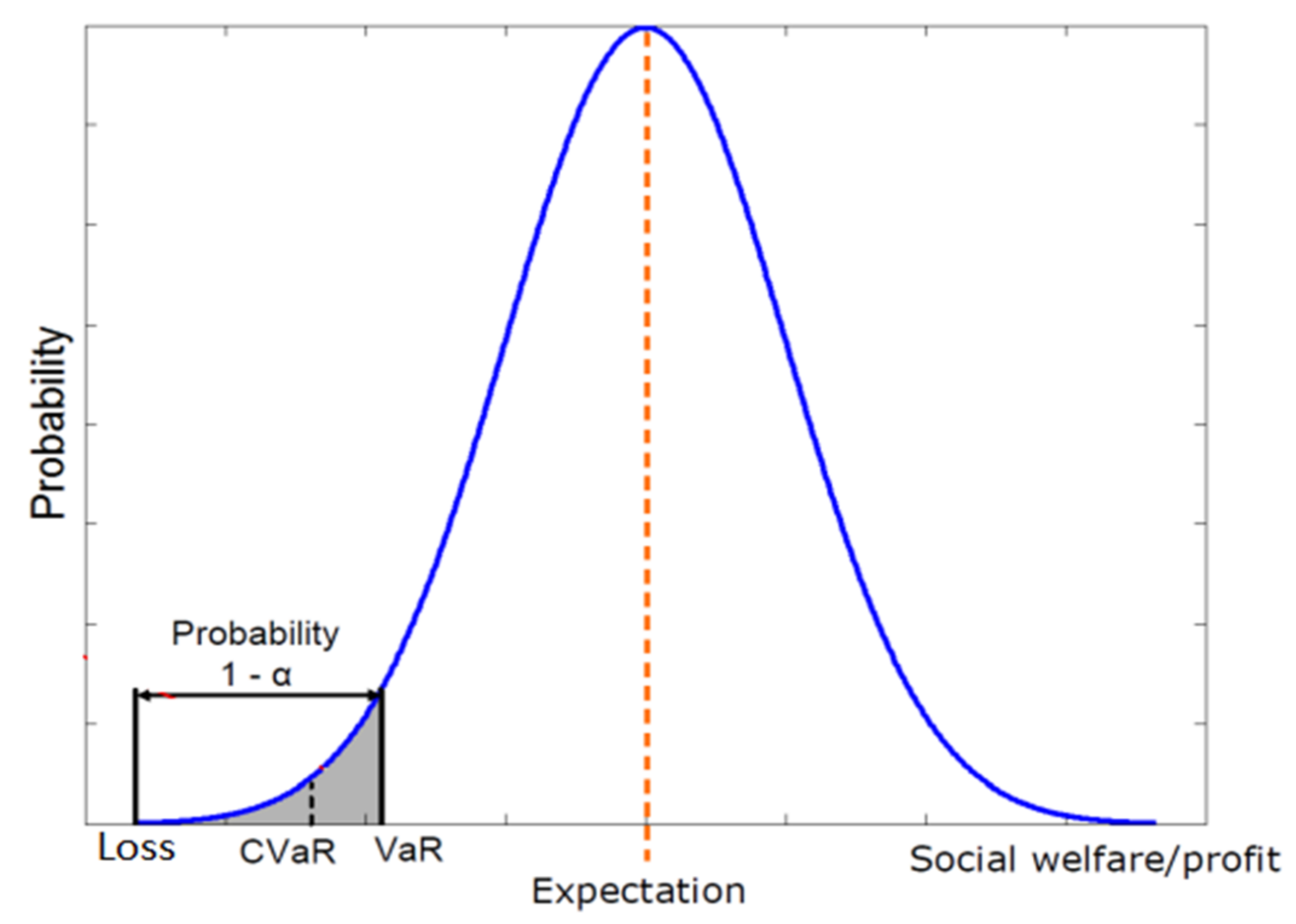
The connection between VaR and CVaR related to the system profit and loss is represented in Figure 1. The sharing of profit and losses is associated with the said relationship. There are two sides to the graph, one is the negative side and the other one is the positive side, where the first side represents the maximum loss and lowest amount of profit and the other side represents the reverse situations. When system loss falls under the utmost condition (system profit is the least amount) then the value of VaR and CVaR is highly negative. Therefore, sequentially when the system loss is under the minimum rate (system profit is maximum) then the value of VaR and CVaR is going to be positive, which is shown by the right region of Figure 1.
2.2. Sequential Quadratic Programming (SQP)
If the problem is related to nonlinearity then Sequential Quadratic Programming (SQP) is one of the most effective methods to obtain the solution. This method generates step-by-step problem formulation and solution by using the quadratic sub-problems process. Line search process and trust-region framework process are used here. SQP method is suitable for solving small problems as well as large problems with a significant number of nonlinearities.
The SQP method is the parallel process of Newton’s method for unconstrained optimization by which it finds a step away from the current point by minimizing a quadratic model of the problem. A number of software packages (MATLAB, NPSOL, NLPQL, OPSYC, OPTIMA, etc.) are based on this approach. SQP is associated with two kinds of algorithms for solving nonlinear problems; they are an active set method and Newton’s method.
Step-by-step process of SQP:
- Step 1: Initializing variables.
- Step 2: Define the search direction of the variables for taken objectives.
- Step 3: Define and solve quadratic programming sub-problems.
- Step 4: Check the optimum result.
- If yes, then go to the next step.
- Otherwise, change search size and repeat from step-2.
- Step 5: Finally, get the best solution.
2.3. Artificial Bee Colony Algorithm (ABC)
Encouraged by the activities of honey bees, an intelligence algorithm was proposed by Karaboga in 2005 named ABC algorithm [39]. A swarm can productively complete jobs through a complete social connection. Three kinds of bees are used in this algorithm i.e., employed bees, onlooker bees, and scout bees. The main job for the employed bees is to search sources of food from the pre-specified food source and share the information about food with the onlooker bees. The best quality food source is selected by onlooker bees. The scout bees are the part of the employed bees that always try to search for new quality food sources [40]. In this algorithm, the employed bees are associated with the first half of the swarm and the second half connected with onlooker bees. The number of results is equal to the number of employed or onlooker bees [41]. This algorithm creates an arbitrarily scattered initial population of NA solutions (source of food), where NA represents the size of the swarm. Let represents the ith solution in the swarm, where the dimension size is D. The employed bees have completed their work by creating a new solution in the surrounding, which as follows:
Here, is an arbitrarily selected solution of candidate , j is an arbitrarily selected dimension index from the set {1,2,…,D} and is an arbitrary number within [−1, 1]. A lucrative selection is selected after the new candidate’s solution . is populated. If the suitable value of . is better than that of its parent , then is replaced by , otherwise the value of remain unchanged. The employed bees share the information about the source of food by waggle dance to the onlooker bees. The information is then verified by the onlooker bees and chooses the correct source of food. The food source chosen procedure is described by:
where is the fitness value of the ith solution of the swarm. If within the limit of the cycle the position is not improved, then the food source is canceled. Let the canceled food source be , then a new source of food is found by the scout bees and replaced by as follows:
where a random number with a range of 0 to 1 is, is the upper boundaries and is the lower boundaries of the jth dimension. The controlling parameters of ABC algorithm used in this work are: no. of onlooker bees, employed bees, scout bees and iteration are 20, 10, 1 and 200, respectively.
Step-by-step process of ABC:
- Step 1: Initializing population and other system variables.
- Step 2: Define and start the employed bee phase.
- Step 3: Define and start the onlooker bee phase.
- Step 4: Check and store the source position of the best food.
- Step 5: Check the availability of Scout bees in the colony?
- If yes, then start the scout bee phase.
- Otherwise, go to the next stage.
- Step 6: Check for the meeting of termination criteria.
- If yes, then go to the next step.
- Otherwise, go to Step 2.
- Step 7: Finally, get the best solution.
The controlling parameters of ABC algorithms used in this work are as follows:
- Number of onlooker bees : 20
- Number of employed bees : 10
- Number of scout bees : 1
- Number of iteration : 200
2.4. Slime Mould Algorithm (SMA)
The slime mould algorithm (SMA) was designed by Shimin Li in 2020 [42]. It is a population-based optimization technique, which works depending on the swinging style of slime-mould in nature. The slime mould refers to the Physarumpolycephalum. The name “slime mould” comes from the concept of fungus. Like other heuristic optimization techniques, some basic stages are performed here also to obtain the optimal result i.e., initialization, calculation of fitness functions, calculation of weight, position updating, and fitness findings.
Usually, Slime mould chooses the food source with the highest concentration based on weight, speed and accuracy. Due to the unique biological characteristics of slime mould, it can utilize a variety of food sources at the same time.
Step-by-step process of SMA:
- Step 1: Initializing population size, iteration numbers, and other system variables.
- Step 2: Define the position of the slime moulds (SM).
- Step 3: Determine the fitness of all presented slime moulds and update the fitness based on the best fitness found.
- Step 4: Update the best position of SM.
- Step 5: Calculate the weight of SM.
- Step 6: Update the positions of SM based on the optimal results.
- Step 7: Get the best fitness value.
- Step 8: Finally, obtain the best solution.
The controlling parameters of SMA used in this work are as follows:
- Population size : 20
- Exploration capability : 0.06
- Exploitation capability : 0.04
- Number of iteration : 200
2.5. Social Benefits
Social benefits (SB) are demarcated as the variance between the customer energy buying price or energy-consuming price to the energy production cost of suppliers [43].
where the profit of the customer C(Pd) and the price of active power generation E(Pg) are considered as:
Here, and are the power-generating source and power-demanding load at bus-i. and are the number of sources and loads present in the system. are the generator cost bid coefficients of the sources (for i = 1, 2, 3, … ) and have the customer cost bid coefficient of the extreme demand of load of bus j.
3. Problem Formulation
From the basic concept of VaR and CVaR, it is clear that the system risk and VaR, CVaR are inversely proportional to each other, i.e., the system risk is maximum when VaR and CVaR is minimum (highly negative). So, it is required to minimize the system risk by shifting the left side point to the right-side point of the graph (shown in Figure 1), i.e., trying to maximize the VaR and CVaR value in a positive direction. The main highlights of this work are stated as:
- (a)
- In the above-said system, several abnormal conditions are considered and the outcomes of the abnormal conditions are evaluated and inspected under the concept of risk assessment tools such as VaR and CVaR. With the help of this, the most abnormal conditions have been identified with the values of VaR and CVaR. This risk assessment tool identifies the most risk-able sections of the systems. We can identify the undesirable lines where we can focus to make the system more reliable.
- (b)
- Risk curtailment has been done using the SMA and ABC optimization techniques. By these techniques, we can minimize the risk on the unstable lines, which are found by the risk assessment tools.
- (c)
- The cost of a system is very important from the operational point of view. The comparison of system generation cost with sequential quadratic programming (SQP), SMA, and ABC optimization techniques has also been incorporated in this work. By the above said three techniques, the system cost is identified which can be used for the economic betterment of the system.
- (d)
- The deregulated power market always tries to give some benefits to the consumer by minimizing the cost of power. From the market point of view, the profit to the consumer is going to be evaluated on the above-said system. Consumers are always put in the advantageous section by the deregulated power market system, as they have the choice to choose the power from the market as their requirement.
- (e)
- The solar power with energy storage (i.e., Batteries) system has also been incorporated in this work to curtail the system risk. Solar PV has been placed randomly in the test system. Solar PV with battery storage increases the overall reliability and stability of the system by a continuous supply of power.
In this work, two objectives have been considered. The main objective of this work is to minimize the system risk by maximizing the value of VaR and CVaR (i.e., shifting the values of VaR and CVaR from negative to positive). The mathematical expression of the objective functions is as follows:
![Electronics 11 01251 i003]()

If the value of VaR and CVaR is maximized then the system risk is automatically minimized. The second objective of this work is the maximization of social benefit in consideration of the market environment.
For calculating the system generation cost, social benefits, system loss, etc., the optimal power flow (OPF) solution must be solved. Two types of constraints are considered while solving the above objective functions.
3.1. Equality Constraints
Equality constraints are constraints that always have to be enforced. That is, they are always “binding”. For example in the OPF the real and reactive power balance equations at system buses must always be satisfied (at least to within a user-specified tolerance); likewise the area mega-watt (MW) interchange constraints. In contrast, inequality constraints may or may not be binding. For example, a line MVA (i.e., mega volt-ampere) flow may or may not be at its limit, or a generator’s real power output may or may not be at its maximum limit. We bind our results under some constraints in practical cases.
Equations (14) and (15) represent the real power balance equation whereas Equations (16) and (17) represent the power flow equations. is the line conductance between the bus i and j. The voltage magnitude is represented by , of bus i, j and k, respectively. The voltage angle is represented by , and of the bus i, j and k. The real and reactive power is and which is flows through the system through the bus i. and are the magnitude and angle of the element in ith row and kth column of the bus admittance matrix.
3.2. In-Equality Constraints
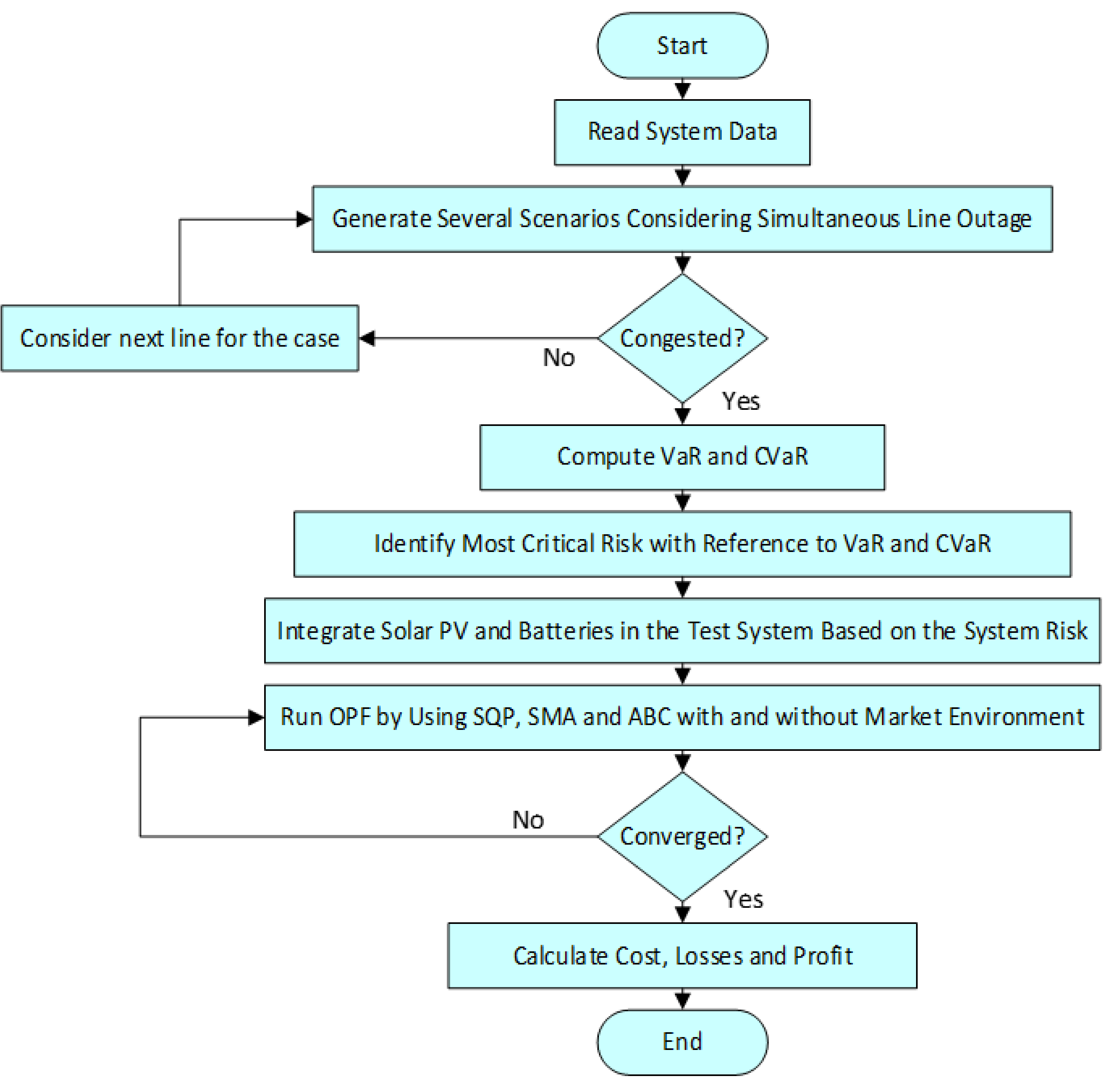
Here, , and , are maximum and minimum limits of real and reactive power correspondingly for bus-i. For bus-i upper voltage and lower voltage limit represents by and and are the upper and lower phase angle limits of voltage for bus-i. The maximum power flow in line-l represents by . The detailed analytic flow chart of the projected method has shown in Figure 2.
Step by step process for solving the presented approach is as follows:
- Read system data.
- Generate several scenarios for checking the efficiency of the proposed approach.
- Compute VaR and CVaR for every scenario.
- Identify the most critical scenarios based on the values of VaR and CVaR.
- Integrate solar PV and batteries with the base system based on the value of VaR and CVaR.
- Perform optimal power flow solution using SQP, SMA, and ABC with and without competitive power environment.
- Calculate system risk, cost, loss, and profit.
4. Results and Discussion
IEEE 14-bus test system and IEEE 30-bus test system are taken here to check the usefulness and stability of the presented approach. The IEEE 14-bus system has five generators, 14 buses, 20 transmission lines, and 10 loads whereas the IEEE-30 bus system consists of six generators, 30 buses, 21 loads, and 41 transmission lines. Bus no. 1 is taken as a reference bus and 100 MVA as base MVA for both systems. The system data have been taken from [44,45]. The OPF problem has been solved in this work to obtain the highest operating levels for electric power plants to meet the desired load throughout a transmission network. Several steps are introduced in this work to obtain the desired objective functions. This work has been done with IEEE 14-bus and IEEE 30-bus systems simultaneously. All the steps associated with this work are done for both test systems simultaneously.
4.1. Step 1: System Risk and Transmission Congestion in IEEE 14-Bus System
The guaranteed prediction of power generation and demand is not possible at all. The power demand is varying every time. Considering this real-time situation, 100 numbers of scenarios have been generated for checking the congestion and risk of the system. All the said scenarios have been generated by performing the interruption of transmission lines (TL), outage of loads, or varying loads in the system. Almost 30 nos. of scenarios with the highest level of risk are identified among all taken conditions. The identification of the degree of risk of the selected scenarios depends on computed values of VaR and CVaR on each case over the systems. At first, VaR and CVaR have been calculated for the base case condition. At that condition, the values of VaR and CVaR are −0.96437 and −1.01513, respectively. After that, several scenarios have been generated by creating some abnormalities in the power system.
Table 1 represents the top five critical scenarios with values of risk assessment parameters (VaR, CVaR) as well as the status of congestion of the system after creating several abnormalities in the system. Depending upon the value of VaR and CVaR it is observed that the no. of the congested TL is maximum where the values of VaR and CVaR are highly negative. The system stability is inversely proportional to the risk assessment tools value so, when the tool’s values are negative maximum, the system becomes more unstable as described in Figure 1.
After finding the values of VaR and CVaR as well as conditions of congested TLs, the rank has been made for all considered scenarios based on the value of risk assessment parameters. Here, the tools assurance level (ɷ) is considered as 95%. So as the value of tools is decreased, the no. of violation lines also tends to decrease. If considering the worst two cases (selected based on the value of VaR and CVaR), then it is found that the line outage of 05–06 and 04–09, respectively, create the highest risk in the system. For the rank-2 scenario, the risk assessment tool’s values are reduced further than the rank-1 case, and no. of line violating has also been reduced.
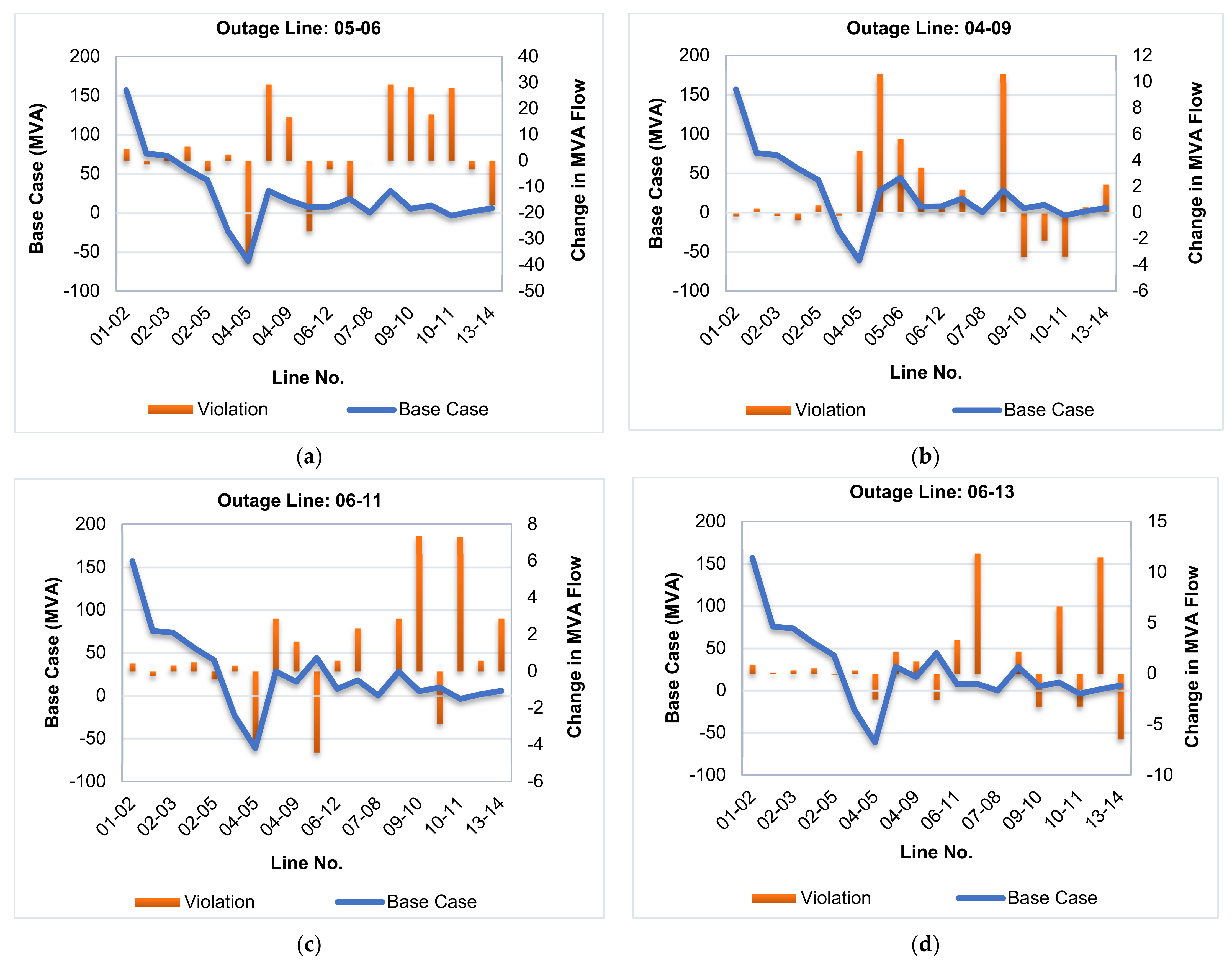
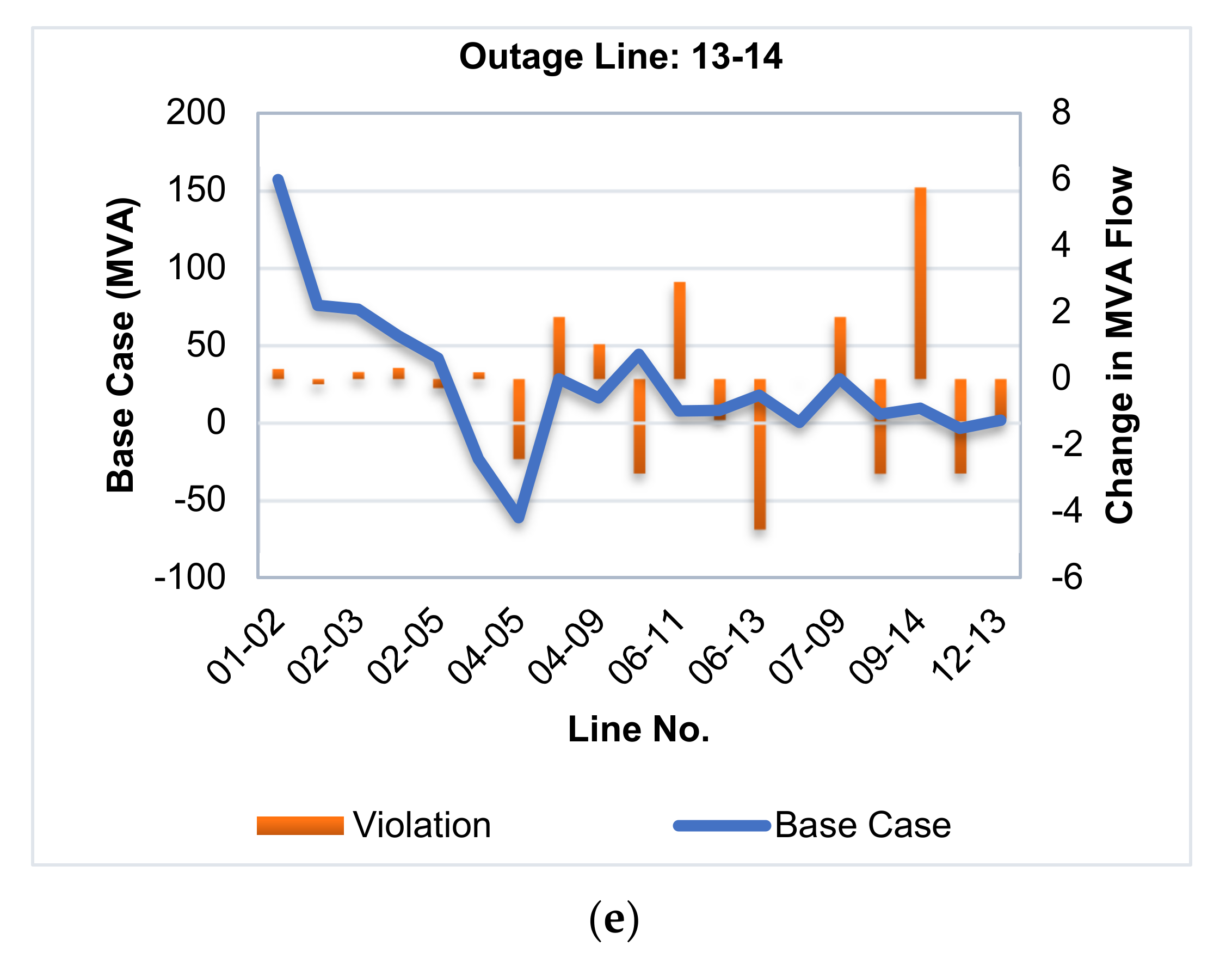
Figure 3 shows the violated values in the several transmission lines in the IEEE 14-bus system after creating the system abnormalities. In normal conditions, every transmission line has a specific maximum thermal limit for power flow. If any fault or abnormality has occurred in the system, then many TLs are carrying their maximum limited power or higher values, which results in the creation of congestion in the system. The power flows in the normal conditions (i.e., base case) and power violations in congestion conditions for the top five risk scenarios in the IEEE 14-bus system are depicted in Figure 3.
4.2. Step 2: System Risk Curtailment in IEEE 14-Bus System
Table 2 represents the system risk analysis result with the application of some risk curtailment techniques. The top two most (i.e., outage of line 05–06 and 04–09) and top two least (i.e., outage of line 04–07 and 04–05) system risk conditions have been taken to check the usefulness of the proposed approach. SQP, SMA and ABC optimization techniques are applied in this work for comparative study. This work is the first attempt in this entire field of the power system to mitigate the system risk by using these optimization techniques.
From Table 2, it is clear that the values of VaR and CVaR are reduced after the incorporation of SMA and ABC for all four taken cases. For the case of line outage of 05–06, the value of VaR and CVaR by using SQP is −0.9825 and −1.0917, which is reduced remarkably after applying the SMA and ABC. The generation cost and loss are also minimum when the SMA and ABC optimization techniques have been used compared with SQP. Therefore, the application of a meta-heuristic algorithm reduces the system risk value, which makesthe system more stable. The deregulated environment has not been considered for this case. For both good and worse cases, the trends of the result are the same irrespective of system risk, system generation cost, and system loss.
Nowadays, global optimization problems have become popular, as a branch of mathematics and computational science, global optimization aims to find the maximum or minimum best solutions. Due to strong search ability, the optimization algorithm can jump out of the local optimum solution and converge to a feasible solution with a small gap to the global optimal solution, which is tolerable in practical application. However, sequential quadratic programming approach gives the local optimal solution instead of the global optimal solution for each sub-problem. Moreover, optimization algorithms give fast responses as compared to the sequential quadratic programming method.
4.3. Step 3: System Risk Curtailment for IEEE 14-Bus System under Deregulated Environment
Deregulation has been done in this work to obtain a competitive market environment. Like the previous case study (i.e., Table 2), in this case, SMA and ABC optimization techniques also provide better results for all the taken scenarios. The most important thing is that after the incorporation of the SMA and ABC algorithm in a deregulated power system, the social benefit, as well as system losses have improved for every case. Table 3 shows the system risk analysis result with the application of SQP, SMA, and ABC techniques with the deregulated market environment. The system loss was 9.77 MW, 9.67 MW, and 9.69 MW for the scenario created by the outage of the transmission line between buses 5–6 without considering the deregulation which is improved after the implementation of deregulation. In this work, four case studies trends have been shown out of that two case studies have performed for worst cases and two case studies for good cases.
4.4. Step 4: Environment System Risk and Transmission Congestion in IEEE 30-Bus System
Like the IEEE 14-bus system, the system risk has been calculated for the IEEE 30-bus system using the risk assessment tools (i.e., VaR and CVaR). Among the 100 taken cases, 30 most critical cases have been chosen based on the value of VaR and CVaR. The most negative higher values of VaR and CVaR indicate the largest risk scenario in the system. All the scenarios have been produced by performing several abnormalities in the system. At first, VaR and CVaR have been calculated for the base case condition. At that condition, the values of VaR and CVaR are −0.96437 and −1.01513, respectively. After that, several scenarios have been generated by creating some abnormalities in the power system. Table 4 signifies the top 10 critical scenarios with values of risk assessment parameters (VaR, CVaR) as well as the status of congestion of the system after creating several abnormalities in the system. Depending upon the value of VaR and CVaR it is observed that the no. of the congested TL is maximum where the values of VaR and CVaR are highly negative.
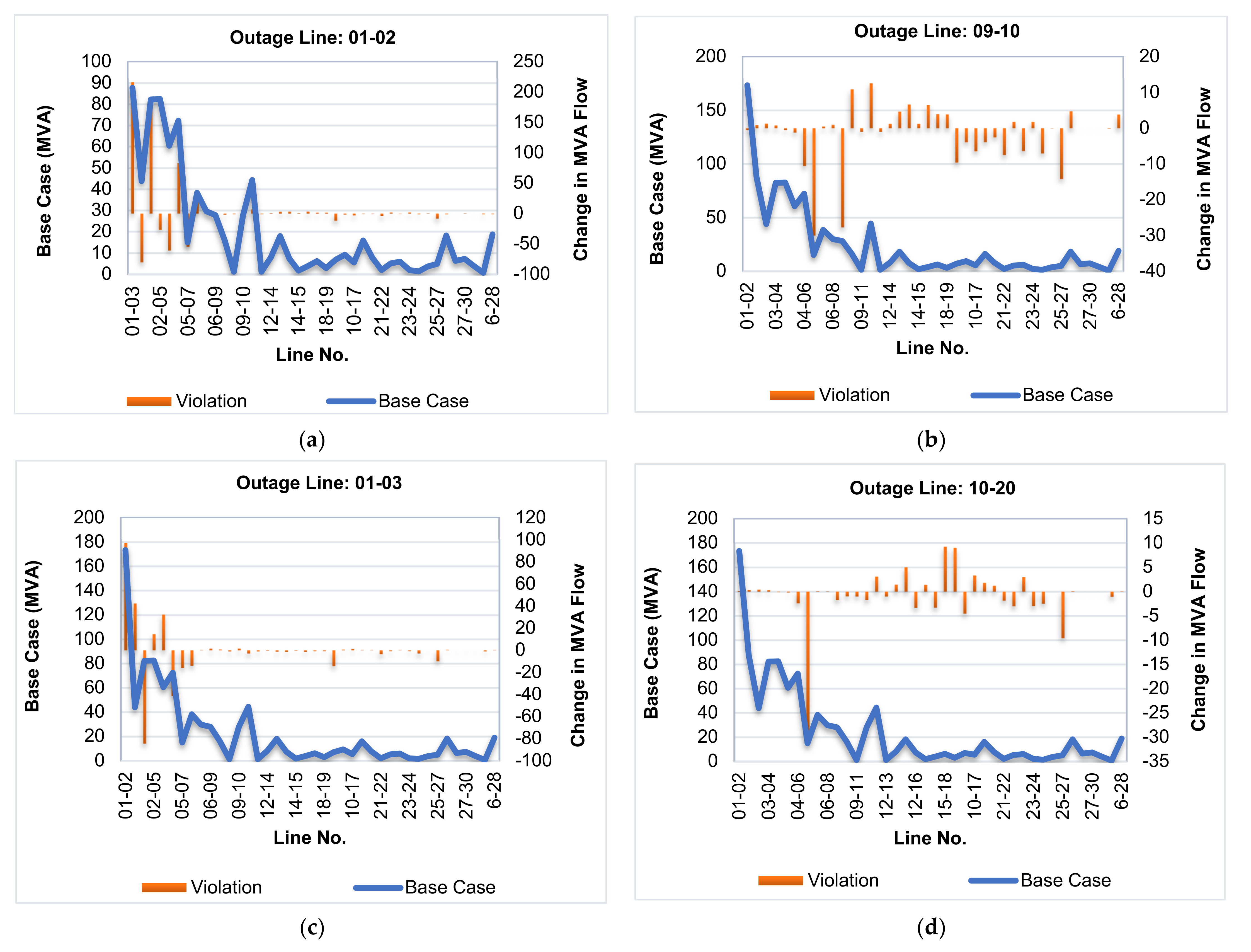
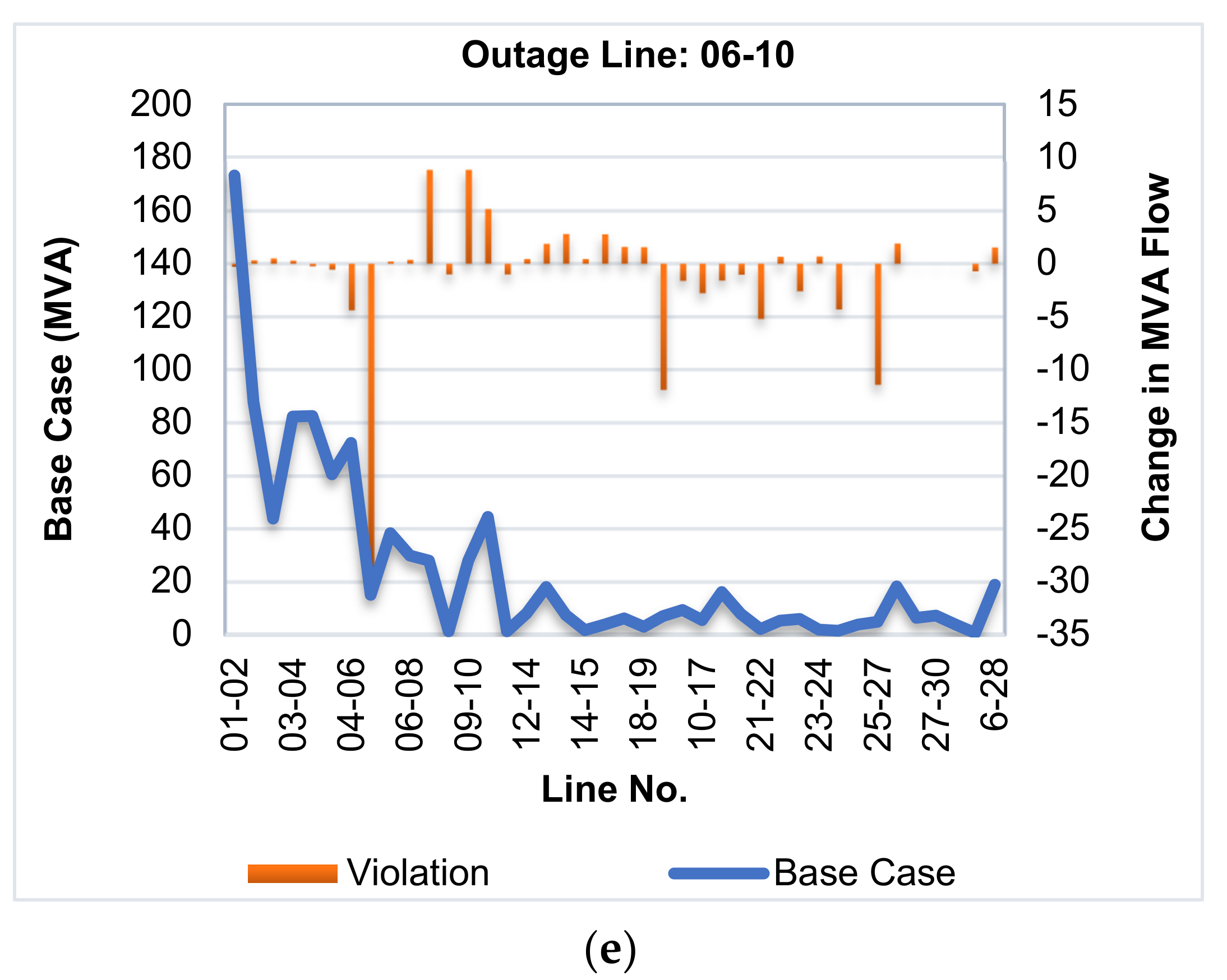
Figure 4 shows the congested values in the several transmission lines in the IEEE 30-bus system after creating the system abnormalities. The power flows in the normal conditions (i.e., base case) and power violations in congestion conditions for the top five risk scenarios in the IEEE 30-bus system are shown in Figure 4.
4.5. Step 5: System Risk Curtailment for IEEE 30-Bus System with and without Deregulated Environment
Table 5 and Table 6 show the optimal results with system risk without and with market environment, respectively, for the IEEE 30-bus system. Like the IEEE 14-bus system, the SMA and ABC algorithms reduce the system risk as well as generation cost, also with an increment of social benefit in the IEEE 30-bus system. The system loss has also improved after the application of SMA and ABC in the worst and best scenarios with and without deregulated environments. In this work, we have taken two worst and two good scenarios among the 100 scenarios for showing the all-around performance of the proposed approach. Table 5 represents the system risk analysis result with the application of some risk curtailment techniques. The top two most (i.e., outage of line 01–02 and 09–10) and top two least (i.e., outage of line 10–17 and 08–28) system risk conditions have been taken to check the usefulness of the proposed approach. From Table 5 it is clear that the values of VaR and CVaR are reduced after the incorporation of SMA and ABC for all four taken cases. For the case of line outage of 01–02, the values of VaR and CVaR by using SQP are−0.9137 and −0.9416 which is reduced remarkably after applying the SMA and ABC.
The generation cost and loss are also minimum when the SMA and ABC optimization techniques have been used compared with SQP. Therefore, the application of SMA and ABC reduces the system risk value, which makes the system more stable.
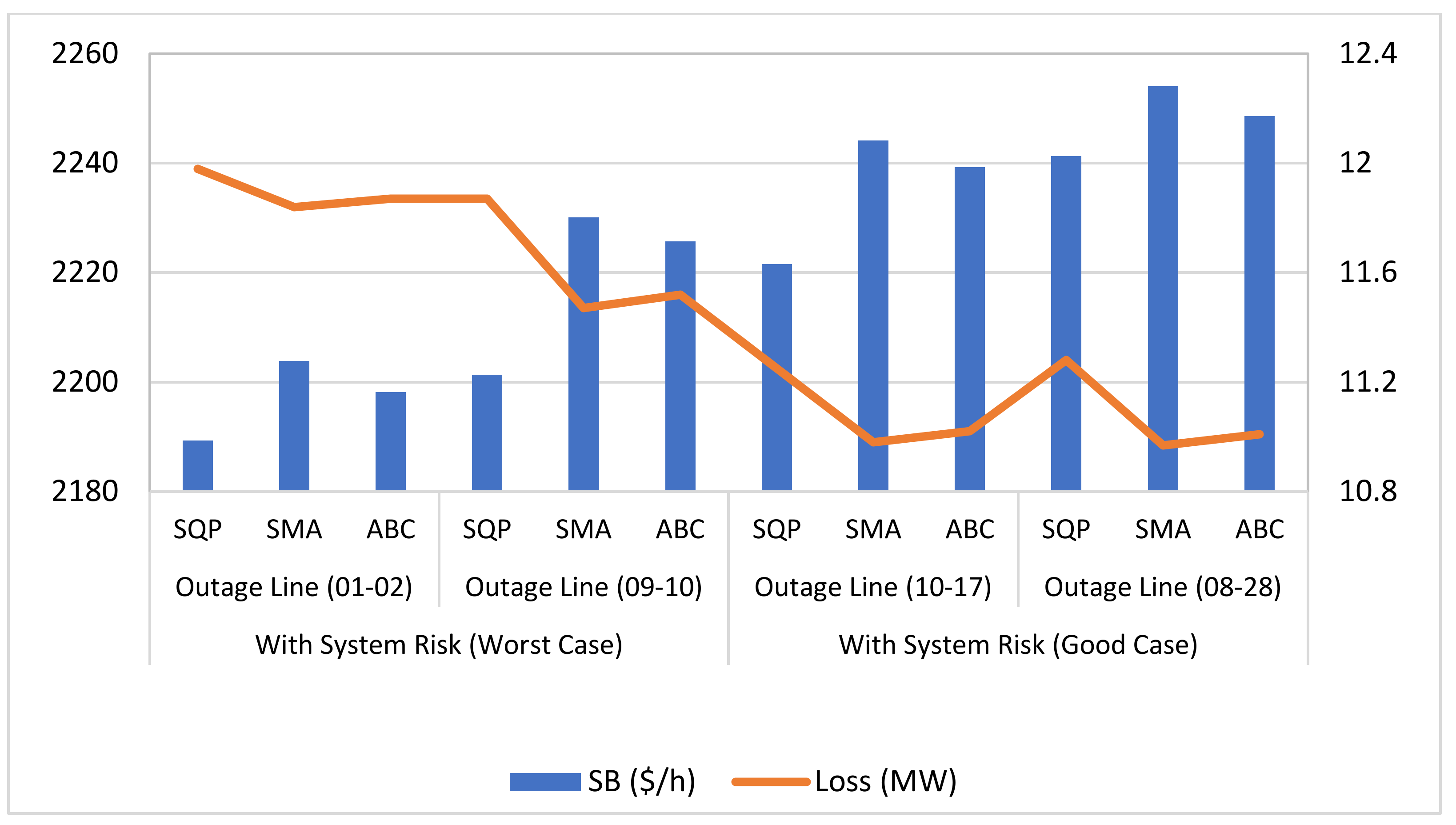
Table 6 shows the system risk analysis result with the application of SQP, SMA, and ABC techniques with the deregulated market environment. The system loss was 12.14 MW, 11.98 MW, and 12.02 MW for the scenario created by the outage of the transmission line between buses 1–2 without considering the deregulation which is improved after the implementation of deregulation (11.98 MW, 11.84 MW, and 11.87 MW). If the transmission loss is minimized, then the system profit will be automatically maximized as well as the social benefit also being maximized.
Figure 5 and Figure 6 show the social benefit and loss considering system risk with and without deregulated environment for the IEEE 30-bus system. The uses of the meta-heuristic optimization technique provide better results in all aspects in both regulated and deregulated power scenarios.
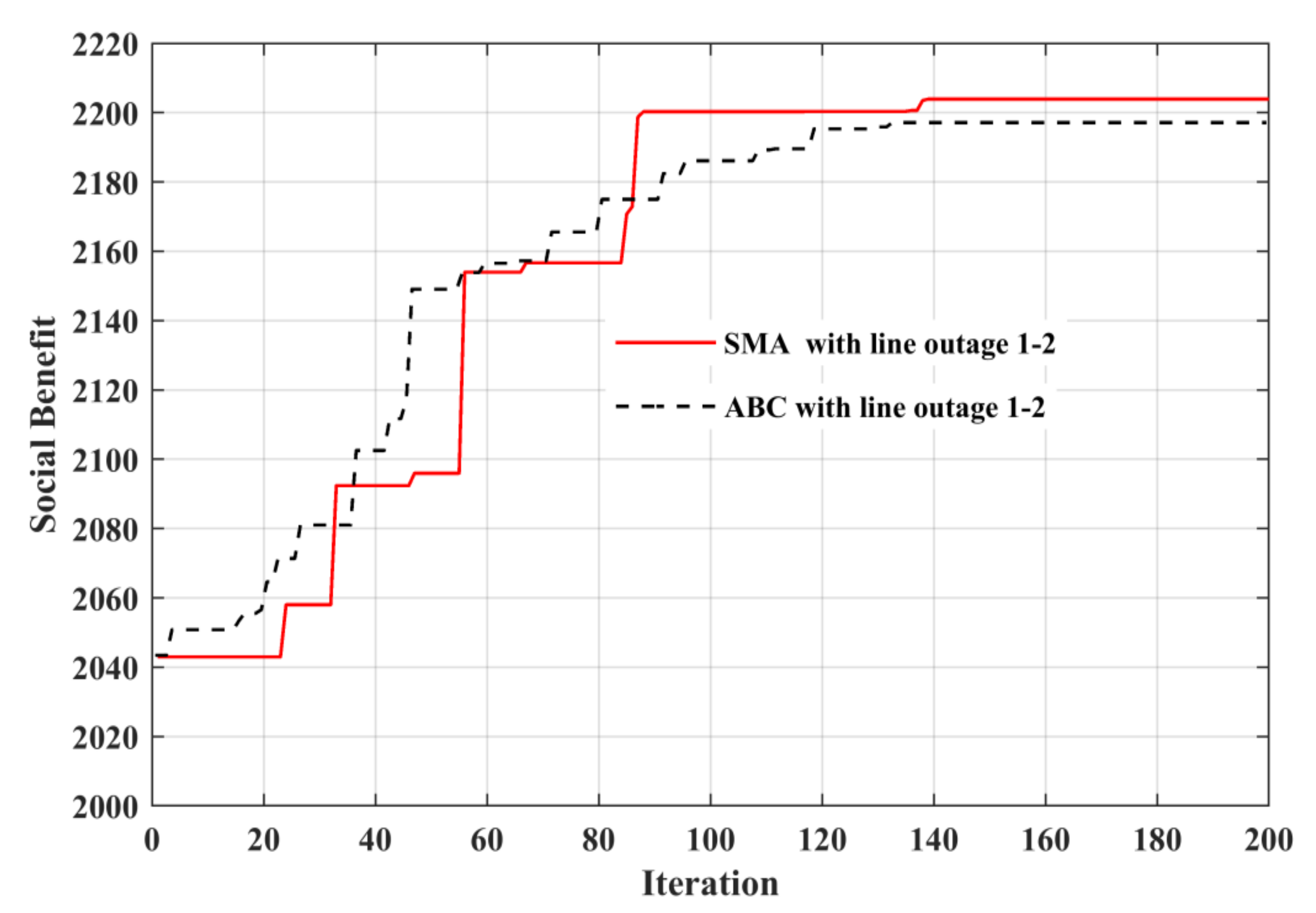
The comparative convergence characteristics under deregulated environment for the line outage of 01–02 in the IEEE 30 bus system is depicted in Figure 7. To solve the problem, programs have been written in MATLAB-18a language and executed on a 2.40 GHz Intel Core i3 processor with 4 GB RAM. The simulation time (in sec.) required for SMA and ABC is 46.65 s and 48.82 s, respectively. The SMA approach is efficient as far as computational time is concerned. Therefore, it can be said that the SMA method is more computationally efficient than the ABC method. However, we have ignored the convergence time for our solution as both the algorithms give almost the same convergence time. Comparisons are made after 50 trials for each implemented algorithm.
4.6. Step 6: System Risk Curtailment Using Renewable Energy Integration in IEEE 14-Bus and IEEE 30-Bus System
Renewable energy integration also plays a vital role in system risk curtailment. Here, Solar PV along with batteries are considered for risk curtailment. Considering the variable power generation nature of Solar PV, two (02) different cases have been considered. A 1.5 MW and 2 MW power supply from Solar PV and battery storage [28] are incorporated in this work.
The placement of the Solar PV and battery storage are taken randomly but they are placed jointly in the system. SQP has been used for solving the Optimal Power Flow problem in this case. Among SQP, SMA, and ABC algorithm techniques, SQP is the less effective technique. Therefore, if the social benefit has been maximized after the placement of solar PV and battery with SQP, then it is very obvious that the SMA and ABC techniques will provide much better results. Table 7 and Table 8 show the values of generation cost as well as VaR and CVaR after placement of Solar PV and battery in IEEE 14-bus and IEEE 30-bus system, respectively.
After the detailed study from Table 7 and Table 8, it can be concluded that renewable energy integration can reduce the system generation cost, which can directly maximize the system profit as well as social benefits. On the other hand, the value of VaR and CVaR has also reduced (i.e., moving towards the positive side of the VaR-CVaR graph) which indicates risk curtailment of the system. If the penetration of solar PV increases, the value of VaR and CVaR will be reduced more. After the detailed studies, it can conclude that the proposed approach can be applied to any large as well as small system.
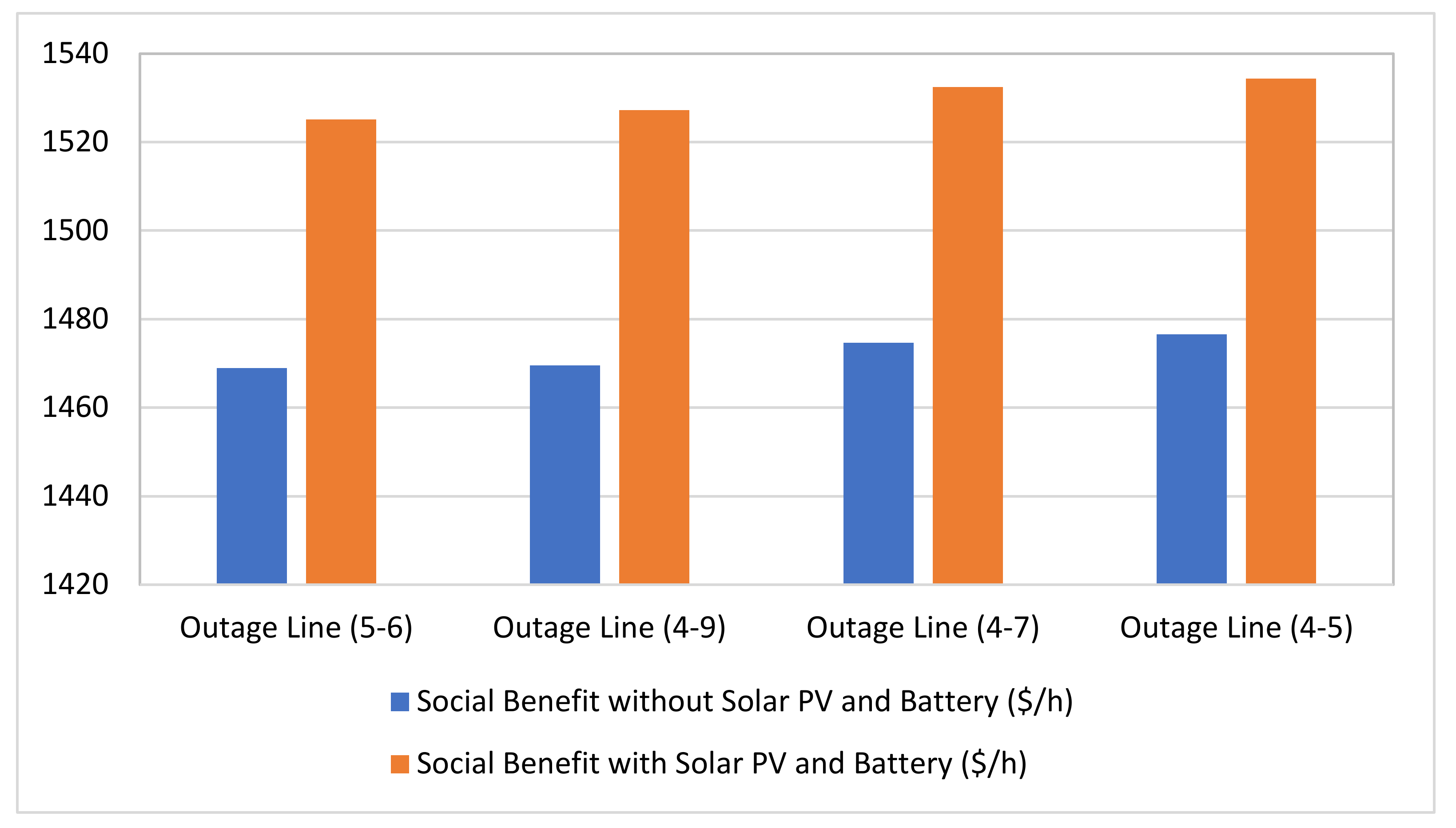
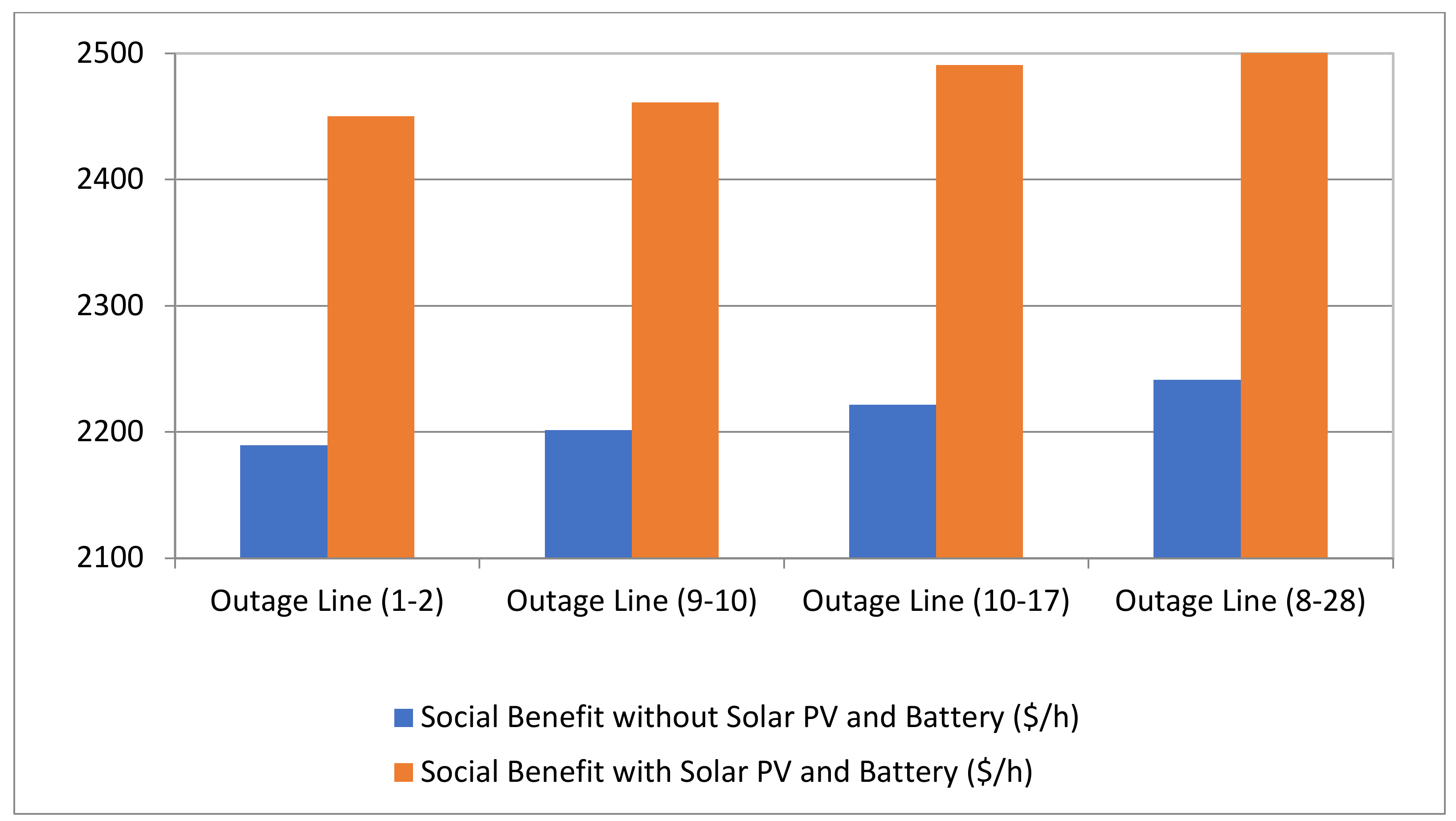
The comparison of social benefits with and without solar PV and battery systems in IEEE 14 bus and IEEE 30 bus system using SQP have been shown in Figure 8 and Figure 9. From these figures, it is clear that the integration of solar PV and battery hybrid systems provides better social benefits for every case using SQP.
The solar PV and battery can provide additional power to the system to fulfill the increased power demand. The renewable energy sources and storage devices can generally deliver the power to the local load first and then excess power is delivered to the grid, so the system loss can be minimized. Therefore, the economic burden to the customers can also be relieved due to the minimization of power generation costs. In this work, we have seen that more power delivered from the backup sources reduced the system risk which happens due to the reduced power flow in the grid. The maximization of social welfare gives economic advancement to the society, which can be further improved by increasing the power supply from renewable energy sources and storage units.
4.7. Step 7: VaR and CVaR Comparison after Installation of Solar PV and Battery with a Different Assurance Level
From Step-1 to Step-6, the assurance level (ɷ) has considered 95%. To check the robustness of the proposed method, the assurance level is now considered as 99%. Table 9 and Table 10 show the comparative analysis of VaR and CVaR after installation of solar PV and battery with the assurance level of 95% and 99% in IEEE 14-bus and IEEE 30-bus system, respectively.
From the results, it can be concluded that the values of VaR and CVaR are increased with higher values of assurance level. However, the placement of solar PV and battery provided the same result scenario for both assurance levels. Therefore, the placement of solar PV and battery is one of the best solutions to mitigate the system risk in a renewable integrated deregulated power system.
5. Conclusions
Power system risk is one of the most important issues in the today’s electricity market. To address the inherent uncertainty of the renewable power generations as well as load demand, VaR and CVaR may be utilized to realize risk management and maintain a balance during this problem. With the help of VaR and CVaR, a high degree of risk may also be identified in the recent power market. This paper described a novel risk curtailment approach considering renewable energy sources integrated with congested transmission systems under a deregulated power market environment. From the analysis, it is evident that the deregulated power market reduces the system risk compared to the normal market environment.
It is also clear from the results that the integration of solar PV and battery storage systems reduces the system risk compared to the normal case. It is observed that the maximum loss can be minimized to a great extent by using the SMA. Social benefits are also increased and that ensures maximum benefits to the consumers. The generation cost under a worst-case and good case is reduced significantly after placing the solar and battery on the system. The study has been conducted on the IEEE 14 bus and IEEE 30 bus systems. For analyzing these results, SQP, SMA, and ABC algorithms are used here. The result shows that the SMA and ABC algorithms give better results in terms of less VaR and CVaR values and maximum social benefit with minimum losses. The SMA algorithms have been used for the first time in this area of work, which is the novelty of this paper. This approach can also be followed for small as well as large systems.
Author Contributions
Conceptualization, A.D. and S.D.; methodology, A.D., S.D., S.G. and T.S.U.; software, S.D. and S.G.; validation, A.D., S.D., S.G. and T.S.U.; formal analysis, T.S.U.; investigation, S.D., S.G. and T.S.U.; resources, A.D., S.D., S.G. and T.S.U.; data curation, T.S.U.; writing—original draft preparation, S.D.; writing—review and editing, T.S.U.; visualization, A.D., S.D., S.G. and T.S.U.; supervision, S.G.; project administration, A.D., S.D., S.G. and T.S.U.; funding acquisition, T.S.U. All authors have read and agreed to the published version of the manuscript.
Funding
This research received no external funding.
Conflicts of Interest
The authors declare no conflict of interest.
Nomenclature
| ɷ | Level of assurance |
| (1 − ɷ) | Distribution of loss quantity |
| m(P,Q) | Loss related with the decision vector P |
| Q | Vector for the unpredictable values |
| Ξ | The threshold value for the probable value of VaR and CVaR |
| Fundamental formation of ɷ-VaR | |
| Fundamental formation of ɷ-CVaR | |
| The unique index | |
| N | Total number of samples accumulated under various conditions |
| n(A,B) | Loss linked to the decision vector A and random vector B |
| C(Pd) | Profit of the customer |
| E(Pg) | Price of active power generation |
| Line conductance between the bus-i and bus-j | |
| , | Voltage magnitude of bus i, j and k |
| , , | Voltage angle of bus i, j, and k |
| , | Real and reactive power flows through the system through bus i |
| , | Magnitude and angle of the element in ith row and kth column of the bus admittance matrix |
| , | Maximum and minimum limits of real power for bus-i |
| , | Maximum and minimum limits of reactive power for bus-i |
| , | Upper and lower voltage limit for bus-i |
| , | Upper and lower phase angle limits of voltage for bus-i |
| Maximum power flow in line-l |
References
- Ustun, T.S.; Hashimoto, J.; Otani, K. Impact of Smart Inverters on Feeder Hosting Capacity of Distribution Networks. IEEE Access 2019, 7, 163526–163536. [Google Scholar] [CrossRef]
- Almesqab, F.; Ustun, T.S. Lessons learned from rural electrification initiatives in developing countries: Insights for technical, social, financial and public policy aspects. Renew. Sustain. Energy Rev. 2019, 102, 35–53. [Google Scholar] [CrossRef]
- Hussain, S.M.S.; Aftab, M.A.; Ali, I.; Ustun, T.S. Optimal Energy Routing in Microgrids with IEC 61850 Based Energy Routers. IEEE Trans. Ind. Electron. 2020, 6, 5161–5169. [Google Scholar] [CrossRef]
- Nadeem, F.; Aftab, M.A.; Hussain, S.M.; Ali, I.; Tiwari, P.K.; Goswami, A.K.; Ustun, T.S. Virtual Power Plant Management in Smart Grids with XMPP Based IEC 61850 Communication. Energies 2019, 12, 2398. [Google Scholar] [CrossRef] [Green Version]
- Gope, S.; Goswami, A.K.; Tiwari, P.K. Transmission congestion management with integration of wind farm: A possible solution methodology for deregulated power market. Int. J. Syst. Assur. Eng. Manag. 2020, 11, 287–296. [Google Scholar] [CrossRef]
- Ustun, T.S.; Nakamura, T.; Hashimoto, J.; Otani, K. Performance analysis of PV panels based on different technologies after two years of outdoor exposure in Fukushima, Japan. Renew. Energy 2019, 136, 159–178. [Google Scholar] [CrossRef]
- Ministry of New and Renewable Energy (MNRE), Year-End Review-DEC 2018. Available online: https://pib.gov.in/Pressreleaseshare.aspx?PRID=1555373 (accessed on 5 January 2022).
- Negnevitsky, M.; Nguyen, D.H.; Piekutowski, M. Risk Assessment for Power System Operation Planning With High Wind Power Penetration. IEEE Trans. Power Syst. 2015, 30, 1359–1368. [Google Scholar] [CrossRef]
- Rockafellar, R.T.; Uryasev, S. Conditional value-at-risk for general loss distributions. J. Bank. Financ. 2002, 26, 1443–1471. [Google Scholar] [CrossRef]
- Dawn, S.; Tiwari, P.K.; Goswami, A.K.; Panda, R. An Approach for System Risk Assessment and Mitigation by Optimal Operation of Wind Farm & FACTS Devices in Centralized Competitive Power Market. IEEE Trans. Sustain. Energy 2018, 10, 1054–1065. [Google Scholar]
- Singh, S.; Prachi, C.; Mohd, A.A.; Ikbal, A.; Suhail, H.S.M.; Taha, S.U. Cost Optimization of a Stand-Alone Hybrid Energy System with Fuel Cell and PV. Energies 2020, 13, 1295. [Google Scholar] [CrossRef] [Green Version]
- Kikusato, H.; Taha, S.U.; Masaichi, S.; Shuichi, S.; Jun, H.; Kenji, O.; Kenji, S.; Rina, Y.; Ken, W.; Tatsuaki, S.M. Controller Testing Using Power Hardware-in-the-Loop. Energies 2020, 13, 2044. [Google Scholar] [CrossRef] [Green Version]
- Li, H.; Xu, B.; Arzaghi, E.; Abbassi, R.; Chen, D.; George, A.A.; Zhang, J.; Patelli, E. Transient safety assessment and risk mitigation of a hydroelectric generation system. Energy 2020, 196, 1–17. [Google Scholar] [CrossRef]
- Yun, S.Y.; Kim, J.C. An evaluation method of voltage sag using a risk assessment model in power distribution systems. Electr. Power Energy Syst. 2003, 25, 829–839. [Google Scholar] [CrossRef]
- Yang, H.; Qiu, J.; Meng, K.; Zhao, J.H.; Dong, Z.Y.; Lai, M. Insurance strategy for mitigating power system operational risk introduced by wind power forecasting uncertainty. Renew. Energy 2016, 89, 606–615. [Google Scholar] [CrossRef]
- Wang, L.; Huang, G.; Wang, X.; Zhu, H. Risk-based electric power system planning for climate change mitigation through multi-stage joint-probabilistic left-hand-side chance-constrained fractional programming: A Canadian case study. Renew. Sustain. Energy Rev. 2018, 82, 1056–1067. [Google Scholar] [CrossRef]
- Shiwen, Y.; Hui, H.; Chengzhi, W.; Hao, G.; Hao, F. Review on Risk Assessment of Power System. Procedia Comput. Sci. 2017, 109, 1200–1205. [Google Scholar] [CrossRef]
- Agwa, A.M.; Hassan, H.M. Onsite power system risk assessment for nuclear power plants considering components ageing. Prog. Nucl. Energy 2019, 110, 384–392. [Google Scholar] [CrossRef]
- Henneaux, P.; Labeau, P.E.; Maun, J.C. A level-1 probabilistic risk assessment to blackout hazard in transmission power systems. Reliab. Eng. Syst. Saf. 2012, 102, 41–52. [Google Scholar] [CrossRef]
- Salman, A.M.; Li, Y. A Probabilistic Framework for Seismic Risk Assessment of Electric Power Systems. Procedia Eng. 2017, 199, 1187–1192. [Google Scholar] [CrossRef]
- Prusty, B.R.; Jena, D. An over-limit risk assessment of PV integrated power system using probabilistic load flow based on multi-time instant uncertainty modeling. Renew. Energy 2018, 116, 367–383. [Google Scholar] [CrossRef]
- Ghazvini, M.A.F.; Lipari, G.; Pau, M.; Ponci, F.; Monti, A.; Soares, J.; Castro, R.; Vale, Z. Congestion management in active distribution networks through demand response implementation. Sustain. Energy Grids Netw. 2019, 17, 100185. [Google Scholar] [CrossRef] [Green Version]
- Jafarian, M.; Scherpen, J.M.A.; Loeff, K.; Mulder, M.; Aiello, M. A combined nodal and uniform pricing mechanism for congestion management in distribution power networks. Electr. Power Syst. Res. 2020, 180, 8. [Google Scholar] [CrossRef]
- Wang, H.; Fang, Y.; Zio, E. Risk Assessment of an Electrical Power System Considering the Influence of Traffic Congestion on a Hypothetical Scenario of Electrified Transportation System in New York State. IEEE Trans. Intell. Transp. Syst. 2021, 22, 142–155. [Google Scholar] [CrossRef]
- Niu, M.; Xu, N.Z.; Kong, X. Reliability Importance of Renewable Energy Sources to Overall Generating Systems. IEEE Access 2021, 9, 20450–20459. [Google Scholar] [CrossRef]
- Kilian, P.; Kohler, A.; van Bergen, P.; Gebauer, C. Principle Guidelines for Safe Power Supply Systems Development. IEEE Access 2021, 9, 107751–107766. [Google Scholar] [CrossRef]
- Yin, F.; Hajjiah, A.; Jermsittiparsert, K.; Al-Sumaiti, A.S. A Secured Social-Economic Framework Based on PEM-Blockchain for Optimal Scheduling of Reconfigurable Interconnected Microgrids. IEEE Access 2021, 9, 40797–40810. [Google Scholar] [CrossRef]
- Xu, S.; Chen, X.; Xie, J.; Rahman, S. Agent-based Modeling and Simulation for the Electricity Market with Residential Demand Response. CSEE J. Power Energy Syst. 2021, 7, 368–380. [Google Scholar]
- Afshar, K.; Ghiasv, F.S.; Bigdeli, N. Optimal Bidding Strategy of Wind Power Producers in Pay-as-Bid Power Markets. Renew. Energy 2018, 127, 575–586. [Google Scholar] [CrossRef]
- Sing, S.; Fozdar, M. Optimal Bidding Strategy with the Inclusion of Wind Power Supplier in an Emerging Power Market. IET Gener. Transm. Distrib. 2019, 13, 1914–1922. [Google Scholar] [CrossRef]
- Das, S.; Basu, M. Day-Ahead Optimal Bidding Strategy of Microgrid with Demand Response Program Considering Uncertainties and Outages of Renewable Energy Resources. Energy 2020, 190, 116441. [Google Scholar] [CrossRef]
- Panda, R.; Tiwari, P.K. Economic Risk-based Bidding Strategy for Profit maximization of Wind Integrated Day-Ahead and Real-Time Double Auctioned Competitive Power markets. IET Gener. Transm. Distrib. 2019, 13, 209–218. [Google Scholar] [CrossRef]
- Yang, Y.; Qin, C.; Zeng, Y.; Wang, C. Optimal Coordinated Bidding Strategy of Wind and Solar System with Energy Storage in Day-ahead Market. J. Mod. Power Syst. Clean Energy 2022, 10, 192–203. [Google Scholar] [CrossRef]
- Xu, C.; He, X. A Fully Distributed Approach to Optimal Energy Scheduling of Users and Generators Considering a Novel Combined Neurodynamic Algorithm in Smart Grid. IEEE/CAA J. Autom. Sin. 2021, 8, 1325–1335. [Google Scholar] [CrossRef]
- Wei, Q.; Liu, D.; Song, Y.L.R. Optimal Constrained Self-learning Battery Sequential Management in Microgrid Via Adaptive Dynamic Programming. IEEE/CAA J. Autom. Sin. 2017, 4, 168–176. [Google Scholar] [CrossRef]
- Tian, G.; Ren, Y.; Feng, Y.; Zhou, M.C.; Zhang, H.; Tan, J. Modeling and Planning for Dual-Objective Selective Disassembly Using and/or Graph and Discrete Artificial Bee Colony. IEEE Trans. Ind. Inf. 2019, 15, 2456–2468. [Google Scholar] [CrossRef]
- Jia, H.; Miao, H.; Tian, G.; Zhou, M.C.; Feng, Y.; Li, Z.; Li, J. Multiobjective Bike Repositioning in Bike-Sharing Systems via a Modified Artificial Bee Colony Algorithm. IEEE Trans. Autom. Sci. Eng. 2020, 17, 909–920. [Google Scholar] [CrossRef]
- Tang, J.; Liu, G.; Pan, Q. A Review on Representative Swarm Intelligence Algorithms for Solving Optimization Problems: Applications and Trends. IEEE/CAA J. Autom. Sinica 2021, 8, 1627–1643. [Google Scholar] [CrossRef]
- Karaboga, D. An Idea Based on Honey Bee Swarm for Numerical Optimization; Technical Report-TR06; Computer Engineering Department, Engineering Faculty, Erciyes University: Talas/Kayseri, Turkey, 2005. [Google Scholar]
- Deb, S.; Gope, S.; Goswami, A.K. Generator rescheduling for congestion management with incorporation of wind farm using Artificial Bee Colony algorithm. Annu. IEEE India Conf. 2013, 1–6. [Google Scholar] [CrossRef]
- Bouakkaz, A.; Haddad, S.; García, J.M.; Mena, A.G.; Castañeda, J.R. Optimal Scheduling of Household Appliances in Off-Grid Hybrid Energy System using PSO Algorithm for Energy Saving. Int. J. Renew. Energy Res. 2019, 9, 427–436. [Google Scholar]
- Li, S.; Chen, H.; Wang, M.; Heidari, A.A.; Mirjalili, S. Slime mould algorithm: A new method for stochastic optimization. Future Gener. Comput. Syst. 2020, 111, 300–323. [Google Scholar] [CrossRef]
- Tiwari, P.K.; Mishra, M.K.; Dawn, S. A two-step approach for improvement of economic profit and emission with congestion management in hybrid competitive power market. Electr. Power Energy Syst. 2019, 110, 548–564. [Google Scholar] [CrossRef]
- Raghuwanshi, S.S.; Arya, R. Economic and Reliability Evaluation of Hybrid Photovoltaic Energy Systems for Rural Electrification. Int. J. Renew. Energy Res. 2019, 9, 515–524. [Google Scholar]
- Dawn, S.; Tiwari, P.K.; Goswami, A.K. A Joint Scheduling Optimization Strategy for Wind and Pumped Storage Systems Considering Imbalance Cost & Grid Frequency in Real-Time Competitive Power Market. Int. J. Renew. Energy Res. 2016, 6, 1248–1259. [Google Scholar]
Figure 1.
Risk assessment tools representation [10].
Figure 1.
Risk assessment tools representation [10].

Figure 2.
Analytic flow chart of the projected method.

Figure 3.
Different congestion scenarios in IEEE 14-bus System.


Figure 4.
Different congestion scenarios in IEEE 30-bus System.


Figure 5.
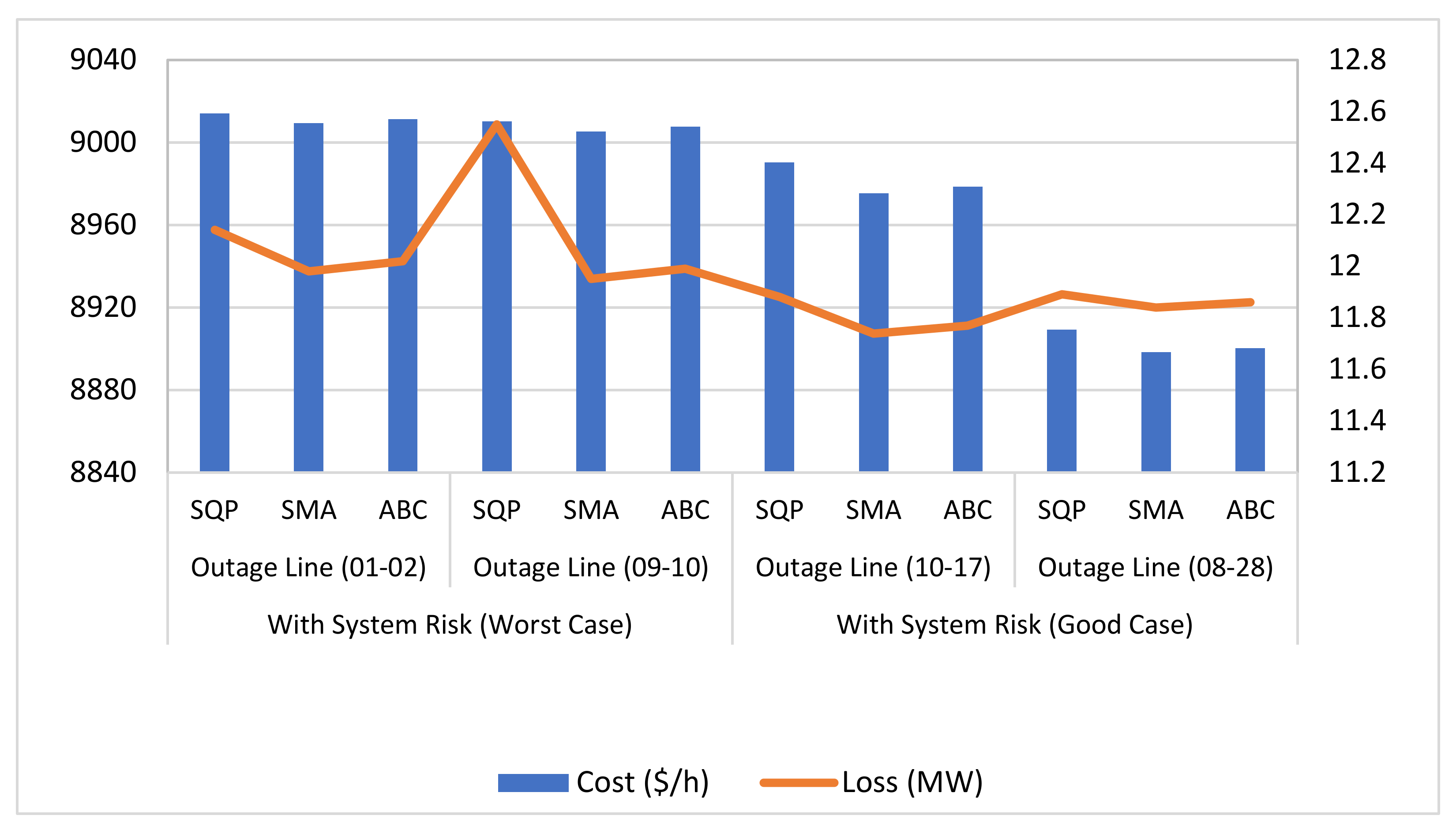
Optimal cost and loss values considering system risk for IEEE 30-bus systems.

Figure 6.
Social benefit and loss considering system risk under deregulated environment for IEEE 30-bus systems.
Figure 6.
Social benefit and loss considering system risk under deregulated environment for IEEE 30-bus systems.

Figure 7.
Comparative convergence characteristics under the deregulated environment in IEEE 30 bus system.
Figure 7.
Comparative convergence characteristics under the deregulated environment in IEEE 30 bus system.

Figure 8.
Social benefit with and without solar PV and battery system in IEEE 14 bus system using SQP.
Figure 8.
Social benefit with and without solar PV and battery system in IEEE 14 bus system using SQP.

Figure 9.
Social benefit with and without solar PV and battery system in IEEE 30 bus system using SQP.
Figure 9.
Social benefit with and without solar PV and battery system in IEEE 30 bus system using SQP.


Table 1.
Congestion and system risk in IEEE 14-bus system.
| Sl. No. | Outage Lines | Risk Assessment | Details of the Congested TL | No. of Congested TL | Rank | |
|---|---|---|---|---|---|---|
| VaR | CVaR | |||||
| 1 | 05–06 | −0.98257 | −1.09175 | 1–2, 1–5, 2–3, 4–5, 4–7, 4–9, 6–11 | 07 | 1 |
| 2 | 04–09 | −0.97411 | −1.08235 | 1–2, 1–5, 2–3, 4–5, 5–6, 7–9 | 06 | 2 |
| 3 | 06–11 | −0.96767 | −1.0752 | 1–2, 1–5, 2–3, 4–5 | 04 | 3 |
| 4 | 06–13 | −0.96695 | −1.07439 | 1–2, 1–5, 2–3, 4–5, 12–13 | 05 | 4 |
| 5 | 13–14 | −0.96659 | −1.074 | 1–2, 1–5, 2–3, 4–5 | 04 | 5 |
Table 2.
Optimal cost and loss values with considering system risk for IEEE 14-bus systems.
| Control Variable | With System Risk (Worst Case) | With System Risk (Good Case) | ||||||||||
|---|---|---|---|---|---|---|---|---|---|---|---|---|
| Outage Line (05–06) | Outage Line (04–09) | Outage Line (04–07) | Outage Line (04–05) | |||||||||
| SQP | SMA | ABC | SQP | SMA | ABC | SQP | SMA | ABC | SQP | SMA | ABC | |
| VaR | −0.9825 | −0.9723 | −0.9745 | −0.7491 | −0.7198 | −0.7256 | −0.7585 | −0.7402 | −0.7469 | −0.9448 | −0.9293 | −0.9326 |
| CVaR | −1.0917 | −1.0753 | −1.0785 | −0.8323 | −0.8103 | −0.8126 | −0.8428 | −0.8202 | −0.8326 | −1.0498 | −1.0298 | −1.0357 |
| Cost ($/h) | 8121.71 | 8099.25 | 8101.61 | 8082.61 | 8063.37 | 8065.58 | 8080.22 | 8076.39 | 8078.69 | 8081.56 | 8079.29 | 8081.02 |
| Loss (MW) | 9.77 | 9.67 | 9.69 | 9.56 | 9.48 | 9.51 | 9.41 | 9.37 | 9.39 | 9.44 | 9.36 | 9.39 |
Table 3.
Social benefit and loss values with considering system risk under deregulated environment for IEEE 14-bus systems.
Table 3.
Social benefit and loss values with considering system risk under deregulated environment for IEEE 14-bus systems.
| Control Variable | With System Risk (Worst Case) | With System Risk (Good Case) | ||||||||||
|---|---|---|---|---|---|---|---|---|---|---|---|---|
| Outage Line (05–06) | Outage Line(04–09) | Outage Line (04–07) | Outage Line (04–05) | |||||||||
| SQP | SMA | ABC | SQP | SMA | ABC | SQP | SMA | ABC | SQP | SMA | ABC | |
| VaR | −0.9435 | −0.9312 | −0.9356 | −0.7098 | −0.7012 | −0.7056 | −0.9132 | −0.9095 | −0.9126 | −0.9118 | −0.9012 | −0.9025 |
| CVaR | −0.9978 | −0.9825 | −0.9854 | −0.8134 | −0.7968 | −0.8026 | −0.9056 | −0.8991 | −0.9045 | −0.8996 | −0.8873 | −0.8897 |
| SB ($/h) | 1468.96 | 1475.67 | 1471.69 | 1469.52 | 1476.89 | 1472.54 | 1474.69 | 1479.68 | 1476.52 | 1476.58 | 1481.26 | 1477.33 |
| Loss (MW) | 9.65 | 9.30 | 9.34 | 9.29 | 9.19 | 9.24 | 9.31 | 9.23 | 9.29 | 9.32 | 9.24 | 9.29 |
Table 4.
System risk and congestion in the IEEE 30-bus system.
| Sl. No. | Outage Line | Risk Assessment | Details of the Congested TL | No. of Congested TL | Rank | |
|---|---|---|---|---|---|---|
| VaR | CVaR | |||||
| 1 | 01–02 | −0.9831 | −0.98952 | 1–3, 3–4, 4–6 | 03 | 1 |
| 2 | 09–10 | −0.98177 | −0.98207 | 1–2 | 01 | 2 |
| 3 | 01–03 | −0.97528 | −0.97685 | 1–2, 2–4, 2–6 | 03 | 3 |
| 4 | 10–20 | −0.97384 | −0.97415 | 1–2 | 01 | 4 |
| 5 | 06–10 | −0.97268 | −0.98214 | 1–2 | 01 | 5 |
| 6 | 03–04 | −0.97172 | −0.97506 | 1–2, 2–6 | 02 | 6 |
| 7 | 12–16 | −0.96639 | −0.97055 | 1–2 | 01 | 7 |
| 8 | 15–18 | −0.96555 | −0.96804 | 1–2 | 01 | 8 |
| 9 | 16–17 | −0.96524 | −0.96877 | 1–2 | 01 | 9 |
| 10 | 02–04 | −0.96506 | −0.97059 | 1–2, 2–6 | 02 | 10 |
Table 5.
Optimal cost and loss values considering system risk for IEEE 30-bus systems.
| Control Variable | With System Risk (Worst Case) | With System Risk (Good Case) | ||||||||||
|---|---|---|---|---|---|---|---|---|---|---|---|---|
| Outage Line (01–02) | Outage Line (09–10) | Outage Line (10–17) | Outage Line (08–28) | |||||||||
| SQP | SMA | ABC | SQP | SMA | ABC | SQP | SMA | ABC | SQP | SMA | ABC | |
| VaR | −0.9137 | −0.9113 | −0.9126 | −0.9283 | −0.9128 | −0.9159 | −0.9621 | −0.9598 | −0.9615 | −0.8727 | −0.8672 | −0.8689 |
| CVaR | −0.9416 | −0.9305 | −0.9326 | −0.9615 | −0.9568 | −0.9589 | −0.9651 | −0.9586 | −0.9598 | −0.9183 | −0.9086 | −0.9155 |
| Cost ($/h) | 9014.12 | 9009.25 | 9011.18 | 9010.26 | 9005.26 | 9007.56 | 8990.23 | 8975.23 | 8978.58 | 8909.29 | 8898.23 | 8900.26 |
| Loss (MW) | 12.14 | 11.98 | 12.02 | 12.55 | 11.95 | 11.99 | 11.88 | 11.74 | 11.77 | 11.89 | 11.84 | 11.86 |
Table 6.
Social benefit and loss values considering system risk under deregulated environment for IEEE 30-bus systems.
Table 6.
Social benefit and loss values considering system risk under deregulated environment for IEEE 30-bus systems.
| Control Variable | With System Risk (Worst Case) | With System Risk (Good Case) | ||||||||||
|---|---|---|---|---|---|---|---|---|---|---|---|---|
| Outage Line (01–02) | Outage Line (09–10) | Outage Line (10–17) | Outage Line (08–28) | |||||||||
| SQP | SMA | ABC | SQP | SMA | ABC | SQP | SMA | ABC | SQP | SMA | ABC | |
| VaR | −0.8999 | −0.8815 | −0.8832 | −0.9015 | −0.8881 | −0.8996 | −0.9002 | −0.885 | −0.9001 | −0.9652 | −0.9498 | −0.9587 |
| CVaR | −0.8990 | −0.876 | −0.882 | −0.9236 | −0.8916 | −0.9026 | −0.8966 | −0.8935 | −0.8959 | −0.9154 | −0.9001 | −0.9026 |
| SB ($/h) | 2189.36 | 2203.9 | 2198.2 | 2201.32 | 2230.08 | 2225.69 | 2221.58 | 2244.12 | 2239.25 | 2241.3 | 2254.05 | 2248.62 |
| Loss (MW) | 11.98 | 11.84 | 11.87 | 11.87 | 11.47 | 11.52 | 11.25 | 10.98 | 11.02 | 11.28 | 10.97 | 11.01 |
Table 7.
VaR and CVaR after Installation of Solar PV and Battery in IEEE 14-bus System.
| Case | Outage Line | Solar PV and Battery Positioning at Bus No. | Power from Solar PV and Battery (MW) | System Generation Cost before Positioning of Solar PV and Battery ($/h) | System Generation Cost after Positioning of Solar PV and Battery ($/h) | Risk Parameter before Positioning of Solar PV and Battery | Risk Parameter after Positioning of Solar PV and Battery | ||
|---|---|---|---|---|---|---|---|---|---|
| VaR | CVaR | VaR | CVaR | ||||||
| Worst Case | 05–06 | 13 | 1.5 | 8121.71 | 8058.08 | −0.9825 | −1.0917 | −0.9735 | −1.0817 |
| 2 | 8037.5 | −0.9732 | −1.0813 | ||||||
| 10 | 1.5 | 8059.91 | −0.9726 | −1.0807 | |||||
| 2 | 8039.94 | −0.9719 | −1.0802 | ||||||
| 04–09 | 13 | 1.5 | 8082.61 | 8021.73 | −0.7491 | −0.8323 | −0.7485 | −0.8302 | |
| 2 | 8001.57 | −0.7469 | −0.8291 | ||||||
| 10 | 1.5 | 8021.76 | −0.7416 | −0.8253 | |||||
| 2 | 8001.61 | −0.7367 | −0.8219 | ||||||
| Good Case | 04–07 | 13 | 1.5 | 8080.22 | 7964.49 | −0.7585 | −0.8428 | −0.7532 | −0.8372 |
| 2 | 7944.42 | −0.7525 | −0.8346 | ||||||
| 10 | 1.5 | 8024.77 | −0.7519 | −0.8317 | |||||
| 2 | 8004.61 | −0.7512 | −0.8302 | ||||||
| 04–05 | 13 | 1.5 | 8082.56 | 7999.32 | −0.9448 | −1.0498 | −0.9378 | −0.9339 | |
| 2 | 7979.58 | −0.9359 | −0.9306 | ||||||
| 10 | 1.5 | 8078.75 | −0.9139 | −0.9278 | |||||
| 2 | 8058.65 | −0.851 | −0.9155 | ||||||
Table 8.
VaR and CVaR after Installation of Solar PV and Battery in IEEE 30-bus System.
| Case | Outage Line | Solar PV and Battery Positioning at Bus No. | Power from Solar PV and Battery (MW) | System Generation Cost before Positioning of Solar PV and Battery ($/h) | System Generation Cost after Positioning of Solar PV and Battery ($/h) | Risk Parameter before Positioning of Solar PV and Battery | Risk Parameter after Positioning of Solar PV and Battery | ||
|---|---|---|---|---|---|---|---|---|---|
| VaR | CVaR | VaR | CVaR | ||||||
| Worst Case | 01–02 | 4 | 1.5 | 9014.12 | 8739.52 | −0.9137 | −0.9416 | −0.9058 | −0.9345 |
| 2 | 8759.26 | −0.9076 | −0.9369 | ||||||
| 7 | 1.5 | 8736.59 | −0.9053 | −0.9341 | |||||
| 2 | 8757.07 | −0.9071 | −0.9376 | ||||||
| 09–10 | 4 | 1.5 | 9010.26 | 8841.63 | −0.9283 | −0.9615 | −0.9142 | −0.9539 | |
| 2 | 8861.44 | −0.9177 | −0.9558 | ||||||
| 7 | 1.5 | 8839.77 | −0.9115 | −0.9572 | |||||
| 2 | 8860.04 | −0.9165 | −0.9578 | ||||||
| Good Case | 10–17 | 4 | 1.5 | 8990.23 | 8832.37 | −0.9621 | −0.9651 | −0.9325 | −0.9556 |
| 2 | 8852.17 | −0.9345 | −0.9564 | ||||||
| 7 | 1.5 | 8830.45 | −0.9475 | −0.9621 | |||||
| 2 | 8850.73 | −0.9502 | −0.9641 | ||||||
| 08–28 | 4 | 1.5 | 8909.29 | 8828.29 | −0.8727 | −0.9183 | −0.8421 | −0.9102 | |
| 2 | 8848.06 | −0.8526 | −0.9112 | ||||||
| 7 | 1.5 | 8826.28 | −0.8584 | −0.9012 | |||||
| 2 | 8846.55 | −0.8588 | −0.9045 | ||||||
Table 9.
VaR and CVaR Comparison after Installation of Solar PV and Battery with different assurance level in IEEE 14-bus System.
Table 9.
VaR and CVaR Comparison after Installation of Solar PV and Battery with different assurance level in IEEE 14-bus System.
| Case | Outage Line | Solar PV and Battery Positioning at Bus No. | Power from Solar PV and Battery (MW) | Risk Parameter before Positioning of Solar PV and Battery @ Assurance Level of 95% | Risk Parameter after Positioning of Solar PV and Battery @ Assurance Level of 95% | Risk Parameter before Positioning of Solar PV and Battery @ Assurance Level of 99% | Risk Parameter after Positioning of Solar PV and Battery @ Assurance Level of 99% | ||||
|---|---|---|---|---|---|---|---|---|---|---|---|
| VaR | CVaR | VaR | CVaR | VaR | CVaR | VaR | CVaR | ||||
| Worst Case | 05–06 | 13 | 1.5 | −0.9825 | −1.0917 | −0.9735 | −1.0817 | −1.3836 | −2.3956 | −1.3726 | −2.3887 |
| 10 | −0.9726 | −1.0807 | −1.3695 | −2.3815 | |||||||
| 04–09 | 13 | −0.9448 | −1.0498 | −0.9385 | −1.0382 | −1.3415 | −2.3378 | −1.3385 | −2.3295 | ||
| 10 | −0.9316 | −1.0253 | −1.3315 | −2.3234 | |||||||
| Good Case | 04–07 | 13 | −0.7491 | −0.8323 | −0.7432 | −0.8272 | −1.1482 | −2.1292 | −1.1368 | −2.1164 | |
| 10 | −0.7419 | −0.8217 | −1.1319 | −2.1091 | |||||||
| 04–05 | 13 | −0.7585 | −0.8428 | −0.7478 | −0.8339 | −1.1625 | −2.1569 | −1.1557 | −2.1482 | ||
| 10 | −0.7437 | −0.8278 | −1.1509 | −2.1382 | |||||||
Table 10.
VaR and CVaR Comparison after Installation of Solar PV and Battery with different assurance level in IEEE 30-bus System.
Table 10.
VaR and CVaR Comparison after Installation of Solar PV and Battery with different assurance level in IEEE 30-bus System.
| Case | Outage Line | Solar PV and Battery Positioning at Bus No. | Power from Solar PV and Battery (MW) | Risk Parameter before Positioning of Solar PV and Battery @ Assurance Level of 95% | Risk Parameter after Positioning of Solar PV and Battery @ Assurance Level of 95% | Risk Parameter before Positioning of Solar PV and Battery @ Assurance Level of 99% | Risk Parameter after Positioning of Solar PV and Battery @ Assurance Level of 99% | ||||
|---|---|---|---|---|---|---|---|---|---|---|---|
| VaR | CVaR | VaR | CVaR | VaR | CVaR | VaR | CVaR | ||||
| Worst Case | 01–02 | 4 | 1.5 | −0.9621 | −0.9751 | −0.9558 | −0.9645 | −1.4656 | −2.4712 | −1.4539 | −2.4585 |
| 7 | −0.9533 | −0.9541 | −1.4498 | −2.4529 | |||||||
| 09–10 | 4 | −0.9283 | −0.9615 | −0.9142 | −0.9539 | −1.4295 | −2.4602 | −1.4185 | −2.4483 | ||
| 7 | −0.9055 | −0.9427 | −1.4106 | −2.4408 | |||||||
| Good Case | 10–17 | 4 | −0.8727 | −0.9183 | −0.8625 | −0.9056 | −1.3769 | −2.4191 | −1.3685 | −2.4067 | |
| 7 | −0.8575 | −0.8961 | −1.3607 | −2.3985 | |||||||
| 08–28 | 4 | −0.9137 | −0.9416 | −0.9021 | −0.9302 | −1.4098 | −2.4403 | −1.3968 | −2.4296 | ||
| 7 | −0.8984 | −0.9182 | −1.3895 | −2.4216 | |||||||
Publisher’s Note: MDPI stays neutral with regard to jurisdictional claims in published maps and institutional affiliations. |
© 2022 by the authors. Licensee MDPI, Basel, Switzerland. This article is an open access article distributed under the terms and conditions of the Creative Commons Attribution (CC BY) license (https://creativecommons.org/licenses/by/4.0/).
Share and Cite
MDPI and ACS Style
Das, A.; Dawn, S.; Gope, S.; Ustun, T.S. A Risk Curtailment Strategy for Solar PV-Battery Integrated Competitive Power System. Electronics 2022, 11, 1251. https://doi.org/10.3390/electronics11081251
AMA Style
Das A, Dawn S, Gope S, Ustun TS. A Risk Curtailment Strategy for Solar PV-Battery Integrated Competitive Power System. Electronics. 2022; 11(8):1251. https://doi.org/10.3390/electronics11081251
Chicago/Turabian StyleDas, Arup, Subhojit Dawn, Sadhan Gope, and Taha Selim Ustun. 2022. "A Risk Curtailment Strategy for Solar PV-Battery Integrated Competitive Power System" Electronics 11, no. 8: 1251. https://doi.org/10.3390/electronics11081251
Note that from the first issue of 2016, this journal uses article numbers instead of page numbers. See further details here.