Principles of Machine Learning and Its Application to Thermal Barrier Coatings

Liu, Yuan; Chen, Kuiying; Kumar, Amarnath; Patnaik, Prakash

doi:10.3390/coatings13071140

Open AccessFeature PaperEditor’s ChoiceArticle

Principles of Machine Learning and Its Application to Thermal Barrier Coatings

by

Yuan Liu

¹,

Kuiying Chen

^2,*,

Amarnath Kumar

¹ and

Prakash Patnaik

²

¹

TECSIS Corporation, Ottawa, ON K2E 7L5, Canada

²

Structures, Materials Performance Laboratory, Aerospace Research Centre, National Research Council Canada, Ottawa, ON K1A 0R6, Canada

^*

Author to whom correspondence should be addressed.

Coatings 2023, 13(7), 1140; https://doi.org/10.3390/coatings13071140

Submission received: 14 March 2023 / Revised: 7 May 2023 / Accepted: 16 June 2023 / Published: 23 June 2023

(This article belongs to the Special Issue Advances in Thermal Barrier Coatings (TBCs): Materials, Fabrication, Corrosion and Applications)

Abstract

:

Artificial intelligence (AI), machine learning (ML) and deep learning (DL) along with big data (BD) management are currently viable approaches that can significantly help gas turbine components’ design and development. Optimizing microstructures of hot section components such as thermal barrier coatings (TBCs) to improve their durability has long been a challenging task in the gas turbine industry. In this paper, a literature review on ML principles and its various associated algorithms was presented first and then followed by its application to investigate thermal conductivity of TBCs. This combined approach can help better understand the physics behind thermal conductivity, and on the other hand, can also boost the design of low thermal conductivity of the TBCs system in terms of microstructure–property relationships. Several ML models and algorithms such as support vector regression (SVR), Gaussian process regression (GPR) and convolution neural network and regression algorithms were used via Python. A large volume of thermal conductivity data was compiled and extracted from the literature for TBCs using PlotDigitizer software and then used to test and validate ML models. It was found that the test data were strongly associated with five key factors as identifiers. The prediction of thermal conductivity was performed using three approaches: polynomial regression, neural network (NN) and gradient boosting regression (GBR). The results suggest that NN using the BR model and GBR have better prediction capability.

Keywords:

artificial intelligence; algorithms; hot section components; thermal barrier coatings; thermal physical properties; gas turbine engines

1. Introduction

Recent advances in artificial intelligence (AI) emerge from quantum improvements in computational capabilities and ever-growing datasets in almost all domains of science and technology. Over the past two decades, innovations in cloud computing, data infrastructure management and processing and in computation speeds have increased dramatically. Artificial intelligence (AI), machine learning (ML), deep learning (DL) and big data (BD) encompass powerful data processing to augment human decision making with the use of computational algorithms. The algorithm and programming of ML and DL allow computers to learn and extract information from data automatically by computational and statistical models and methodologies. ML and DL can also make it possible to identify trends in machine performance such as anomalies and signatures. Predictive maintenance system (PMS) based on the aviation industry’s big data analysis can monitor failures in gas turbine engines (GTE), schedule maintenance in advance resulting in huge costs savings, and enable original equipment manufacture (OEM) to identify long-term trends and requirements of complex aircraft systems with far more accuracy [1,2,3].

DL mainly involves analyzing non-linear correlation and high dimensional datasets implemented through specifically designed numerical algorithms. DL also makes it possible to develop an understanding of patterns of behavior and estimate efficiencies in a machine. Furthermore, the combination of AI–ML–DL–BD will significantly strengthen digital capability in the gas turbine industry and is expected to play an essential role in investigating degradation of hot section components under adverse environments.

High temperature gas turbine materials in the aerospace industry hold an important place and contribution to modern technological progress. Hot section components of gas turbine engines are yet to exploit and embrace ML/DL/AI technologies. However, recent research initiatives indicate a highly promising impact of AI across the entire domain of materials, structures, processing, multiscale modeling and simulations. Large volumes of aviation industries materials data are available and accessible for AI to explore. The material property data, namely physical, chemical, mechanical, structural, thermodynamic, thermos-physical, image-based, etc., build up the big data resource. ML can couple with big data analytics to discover and design new materials, to improve and modify existing materials, to uncover materials laws and phenomena, and to predict/accelerate new material technology [2,4]. Historically, such material discovery and development work have been through experiment-based trial and error methods and/or the theoretical and computational modeling and simulation approach. Both approaches consume a large amount of time involving considerable uncertainties, huge cost and a long development cycle. ML and DL can accelerate the process efficiently through data-driven analytics and modeling. However, quite a few significant challenges remain before the methodologies could be fully developed through sustained research efforts [5,6].

Our current research initiative is towards the area of hot section components of the gas turbine engine and aims to develop the ML modeling algorithm to predict an important material property. In the hot section of gas turbines engines, high-temperature insulating coatings are necessary to protect engine hardware from degradation and prevent service failure. The coatings will allow a higher gas inlet temperature to achieve higher engine efficiency, reliability and durability. Thermal barrier coatings (TBCs) are thin ceramic layers, generally applied by plasma-spraying or physical vapor deposition techniques, to insulate air-cooled metallic components, namely blades and vanes from high-temperature combustion gases. The TBCs are made of a ceramics-based topcoat, intermetallic bond coat, thermally growth oxide (TGO) and substrates. Low thermal conductivity (TC) of TBC material is of prime importance for effective insulation and lasting service. Many factors are known to influence TCs of TBCs; namely, microstructures (grain size, cracks, porosity and density), TBC thickness, sintering effect, anisotropy and inhomogeneity besides TBC compositions. Recent work has demonstrated the effectiveness of TCs on thermal insulation considering thermal flows and coating thickness. A comparison with two TCs (0.8 W/m-k and 1.5 W/m-k) confirmed that the insulation effect (drop in temperature across the TBC) tends to be more effective with lower TC, higher coating thickness and higher thermal flows. Thin TBCs show 20% lower thermal conductivity than thick coatings. The higher content of porosity in the coating improves phonon scattering and decreases thermal conductivity significantly. Thermal barrier coatings are designed to be porous to exhibit low TC. Three other significant factors controlling the microstructures and TC are bond coat surface roughness, coating particles size and coating temperature and speed [7,8].

Only limited research initiatives have been undertaken with thermal conductivity prediction in aeroengine hardware components using ML and DL. This paper aims at addressing the following aspects as given in two main sections and is expected to make a useful contribution. (1) State of the art review of the current progress and challenges in high temperature materials developments for aeroengines using artificial intelligence technology; (2) capabilities of machine learning and deep learning in material property prediction is presented, where the review and analysis focusses on big data structure, resources and management, various algorithms used for ML and DL and different computational tools; (3) modeling and simulation for developing an ML algorithm for thermal conductivity predictions in thermal barrier coatings. A large dataset comprising thermal conductivity is obtained from the literature for the popularly used 6–8 wt% YSZ TBC, the key associated factors are identified, and lastly an attempt was made to make predictions of TC based on the TBC processing conditions such as ageing temperature and time, coating thickness and TBC compositions.

What sets this work apart is the utilization of machine learning algorithms to predict thermal conductivity values in TBCs. By employing a large dataset and identifying key factors, our approach offers a more accurate prediction of thermal conductivity in TBCs than existing methods. Additionally, the findings of this research can be useful in improving the performance of TBCs and in the development of new TBCs for various industrial applications.

2. Current Status of Machine Learning and Its Application in Materials Design and Development

Demands of modern life coming from various fields have imposed an important and diverse requirement for the development and quick delivery of materials with improved performance and life span. Traditionally, developing new materials involves seven sequential stages, such as discovery, property optimization, design procedure and integration as shown in Figure 1. Mainly due to heavy involvement of time-consuming, high-cost and low-efficiency repetitive laboratory experiments and density functional theory (DFT)-based theoretical studies during this traditional process, it takes a longer time period, typically around one or two decades, to go from primary concept/discovery to the final application of new materials. Other notable factors contributing to this long time duration are the sequential nature of the entire process without feedback or interactions between the initial and/or later stages [9]. Over the last five decades, the advent of digital computers has led to the development of this traditional process being aided by computer simulations that resulted in the reduction of the above time frame from 10–20 years to 14–18 months [10]. Over the last two decades, the appearance of the so-called “big data” prompted materials science researchers to use ML techniques for the design and development of new materials which significantly further reduced the development time and computational costs.

The aforementioned advancements in materials science research and development can be summarized using four paradigms, drawing analogies to the overall evolution of science and technology throughout history [5]. The initial paradigm in science relates to empirical observations made over centuries, analogous to metallurgical observations and trial-and-error experiments in materials science. The second paradigm in science emerged a few centuries ago and involves theoretical developments characterized by the formulation of classical laws, theories and models. In materials science, this paradigm manifests through the establishment of thermodynamic laws. The third paradigm in science emerged with the advent of computers a few decades ago and encompasses computational science, enabling the simulation of complex real-world problems based on theories from the second paradigm. In materials science, computer simulations of materials using DFT and molecular dynamics (MD) exemplify this paradigm. In recent years, the substantial amount of data generated by these three paradigms has given rise to the fourth paradigm, also known as data-driven science, that perfectly unifies the other three paradigms, encompassing theory, experimentation, and computer simulations. Within the fourth paradigms, the study of materials science has given rise to the emergence of machine learning techniques rooted in big data analysis. Similarly, an analogy has been drawn between the advancements in materials research and the industrial revolution, labeling the fourth paradigm of materials research as “Materials 4.0” in parallel with the latest industrial revolution known as “Industry 4.0”. [11].

It is impossible to overstate the importance of the availability of high-quality, data-related materials science for realizing the great benefits offered by the fourth paradigm of materials research or “Materials 4.0”. Realizing this significance of high quality materials data resources, the Materials Genome Initiative (MGI) [12] was launched in 2011 which in collaboration with other stakeholders and big data resources provides multiple avenues to create/collect and store a significant amount of materials data. These initiatives made it possible for scientists and engineers to have ready access to large and high-quality materials databases proving all kinds of information about known materials. Section 2.1 of this paper reviews several databases for materials properties resulting from these initiatives.

To expedite the progress of materials design and development using the fourth paradigm of materials research, the application of machine learning techniques has emerged as a significant force within materials science. Machine learning, a branch of artificial intelligence capable of creating models that can effectively learn from past data and situations, holds great promise for the design and development of new materials. Notably, several notable review articles have recently been published, documenting the impact and advancements in machine learning applications for materials design and development [4,5,13,14,15]. Agrawal and Choudhary [5] present a comprehensive framework for materials informatics and discuss the utilization of data-driven techniques to learn relationships between processing, structure, properties and performance. Mueller et al. [13] offer an extensive overview of machine learning techniques, showcasing various examples of recent applications in materials science and exploring emerging efforts. Hill et al. [16] delve into the challenges and opportunities associated with data-driven materials research, with a particular focus on materials data challenges. Kalidindi et al. [15] present a visionary outlook for data and informatics within the future materials innovation ecosystem. Liu et al. [4] provide an inclusive review of the current research status regarding machine learning applications in material property prediction, new materials discovery and other related fields, discussing the associated research issues and outlining future research directions. Wei et al. [3] offer an extensive review specifically focused on recent machine learning applications in materials science, with a special emphasis on deep learning applications.

One of the main goals of the current study is to conduct an overview of ML methods including ensemble learning and deep learning methods and their applications in different domains of material science, and to show the successful experiences and the common challenges.

2.1. Big Data in Materials Science

The data/material informatics make use of existing high quality material data to discover new materials by employing data driven or machine learning techniques. The usefulness of data/material informatics for material development and commercialization was also envisioned by the Materials Genome Initiative (MGI) [12], which ultimately led to the emergence of more open access materials science data infrastructures that collect, host and provide material properties of known elements to various interested practitioners. The emerging interest around the use of data driven or ML techniques to accelerate design of advanced materials ultimately led to the transition of data centers into materials discovery platforms such as the Computational Materials Repository, Citrination, Materials Project, Open Materials Database, Marvel NCCR, SUNCAT and AFLOWLIB.

Some of the publicly available materials data resources that contain large numbers of different kinds of materials properties and structures data are summarized in Appendix A Table A1. Appendix A Table A2 provides details on some of the commercially available materials databases that contain information on the structures and property of different kinds of materials.

2.2. Machine Learning Framework for Materials Design and Development

ML encompasses a collection of potent techniques capable of automatically generating models by learning from previous data and experiences. ML has exhibited its potential across various real-world domains, including pattern recognition, data mining, game theory, bioinformatics, finance, and more. Typically, the general ML framework, depicted in Figure 2 [17], can be employed to construct a prediction model using ML. This framework involves several steps: Firstly, gathering extensive and diverse datasets generated through laboratory experiments and computer simulations. Subsequently, data preprocessing methods are applied to select pertinent materials properties and cleanse the data. The dataset is then divided into training and testing sets and is utilized later in the pipeline by the Model Build and Model Validation modules, respectively. Following this, the Feature Engineering module undertakes the extraction of quality features from the raw data, a task that can be very challenging and dependent on the specific application. It is widely recognized that providing well-designed features is critical to developing a high-performing model.

After successfully extracting suitable features, the subsequent step in the ML framework illustrated in Figure 2 involves training a prediction model by selecting an appropriate learning algorithm that suits the specific problem. ML algorithms can be broadly categorized into supervised, unsupervised, semi-supervised and reinforcement learning types. However, for the purpose of this paper, our focus is solely on supervised learning algorithms for the design and development of new materials. Popular supervised learning algorithms include k-nearest neighbors, artificial neural networks, decision trees and support vector machines, among others. Additionally, by training multiple prediction models, it becomes possible to develop an ensemble of models using supervised ensemble learning algorithms. Prominent examples of such ensemble learning algorithms for generating prediction models are random forests and gradient boosting trees.

In the ML application for materials design and development, several crucial steps can be identified from the workflow depicted in Figure 2. These steps include data preparation, feature engineering and the selection of an appropriate ML algorithm for model development. When analyzing materials properties, it is essential to carefully curate the properties used in the analysis since not all properties may be relevant for a specific analysis. Accurate techniques must be employed to ensure a proper selection. Equally important is the task of selecting the ML algorithm, which should be based on the nature of the specific task and the features present in the dataset. This step also requires careful consideration to ensure the most suitable algorithm is chosen.

2.2.1. Classes of ML Problems

The most common problems tackled by ML techniques are classification, regression, clustering, input/feature selection and anomaly detection. In classification problems, ML builds classifiers or classification models that label given objects into one or more classes. In regression problems, ML techniques are used to build prediction models to output values for some continuous response variable. In clustering problems, ML techniques are used to group objects into different categories based on their similarity measure. ML methods are effective in solving the input/feature selection problem which concerns selecting the smallest subset of inputs/features from all available inputs/features that are necessary to enhance the prediction performance. In anomaly detection, ML methods are used to build computational models to identify or detect novel or outlier objects/events. This paper on ML applications for materials design and development will focus only on the first three problems, namely, classification, regression and clustering.

Supervised learning is by far the most widely used learning type in ML applications. In supervised learning, all the training data instances have target outputs which are labeled with an aim to “teach” or train a model using the labeled data so that it can make accurate predictions on new data instances. Classification and regression problems are generally solved using supervised learning algorithms. In unsupervised scenarios, the training instances have no labels associated with their target output, and the goal is to discover groups or some inherent distributions within the data. Clustering problems are typically solved using unsupervised learning algorithms. In semi-supervised learning, only some of the training data instances have labels for their target outputs, and the remaining data instances, which are typically a major part of the whole training dataset, are not labeled. In reinforcement learning, the traditional approach of providing explicit error feedback to guide the model in generating correct outputs is replaced by using reinforcement signals obtained through interactions with the environment. These reinforcement signals are utilized to evaluate the quality of the generated outputs, enabling the system to learn and enhance its strategies for adapting to the environment.

2.2.2. Feature Engineering and Dimension Reduction

It is well known that the classic ML methods require carefully designed features to achieve good generalization performance. Therefore, feature engineering which is conducted manually is a very important step in the workflow of the traditional ML process. As discussed later, deep learning techniques alleviate this problem by automating this feature engineering step. In materials science, the features are also called descriptors.

Like any ML problem, the selection of crucial features or descriptors that exhibit a strong correlation with the desired material property is a significant step in the feature engineering process and is performed prior to model selection and training as illustrated in Figure 2. An effective material descriptor should satisfy three essential criteria: it should provide a distinct characterization of the material, demonstrate sensitivity towards the target property and be easily obtainable [6].

The main motivation for performing input selection or dimension reduction is to realize the following potential benefits: (a) providing better understanding of the underlying process/model by facilitating data visualization and data understanding, (b) improving efficiency by reducing measurement, storage and computation (model training and utilization) costs, and (c) improving prediction performance. Improved predictive performance due to dimensionality reduction can be obtained by tackling the following issues: (i) using too many input variables reduces predictive performance due to model overfitting, (ii) irrelevant and redundant features can confuse learning algorithms, and (iii) input selection can help to defy the curse of dimensionality to deal with limited training data.

In the extensive material databases discussed in Section 2.1, it is important to acknowledge that the available materials data often exhibit high correlation among themselves. Hence, in many instances, it becomes necessary to employ dimensionality reduction techniques to preprocess the high-dimensional datasets before constructing ML models. Several dimensionality reduction algorithms [18], such as principal component analysis (PCA), multidimensional scaling (MDS) and linear discriminant analysis (LDA), are available to reduce the dimensionality of the feature space. These techniques aid in identifying the most relevant descriptors (or key features) that exhibit a strong correlation with the target material property.

2.2.3. ML Algorithms

In this subsection, the most used shallow learning type of machine algorithms for materials science applications are described by giving brief details on their algorithmic working principles followed by a few of application case studies from the materials science literature. In the subsequent subsections, ensemble learning, and deep learning type algorithms will be described.

k-Nearest Neighbor (kNN) Method

The k-nearest neighbor (kNN) algorithm is used as a multivariate non-parametric method for both regression and classification tasks in ML applications. The kNN method is often called the k-nearest neighbor classifier when it is used for classification problems, while it is called k-nearest neighbor regression when it is applied for regression problems involving prediction of continuous outputs. The kNN method is a memory-based approach without requiring an explicit model and its associated training process; instead the entire training dataset is stored and then is used for the prediction of the new output response whenever a new unseen data instance is presented [19]. This kNN procedure can be described as follows: For a given unseen data instance, the kNN algorithm identifies the k data instances from the training set that are most similar or closest (nearest neighbors) to the unseen data instance. The similarity measure between a new unseen data instance and the nearest neighbors can be defined by any of several distance metrics such as the Euclidian distance in the input or feature space [19]. Then, the unseen data instance is going to be classified to the majority class among the k nearest neighbors for classification problems; while for regression problems, the unseen data is going be assigned the average value or weighted average of the k nearest neighbors.

A diverse dataset of organic molecules was utilized to apply the kNN modeling technique for predicting melting points [20]. The investigation into the influence of the number of nearest neighbors involved the combination of information from these neighbors using different methods. This exploration provided valuable insights into the applicability of the “molecular similarity principle,” which forms the foundation for the kNN method in predicting materials properties. Four distinct methods, including arithmetic and geometric averages, inverse distance weighting and exponential weighting, were tested to predict based on the melting temperatures of the nearest neighbors. The results indicated that the exponential weighting scheme produced the most accurate outcome. The kNN classifier was investigated by Rahim et al., [21] to classify the materials non-destructively tested according to their mechanical properties. The classification results from the study show the kNN classifier giving the accuracy more than 99% which is comparable to the accuracy achieved with the neural network classifier from the same study.

Naïve Bayes Classifier

The naive Bayes classifier, as its name implies, is a simple, yet effective and commonly used ML technique for classification problems. It is a series of simple probabilistic classifiers that make classifications using the maximum a posteriori (MAP) decision rule in a Bayesian setting assuming strong independence between the features. This assumption of strong independence between the features simplifies the computations involved, thus, making this algorithm attractive when the dimension of the feature space is high. While this assumption is generally not satisfied, thus giving credence to the term “naive” in its name, in many practical applications this classifier often outperforms more advanced classifiers [19]. Besides its computational efficiency, the naive Bayes classifier possesses another advantage: it can make classification decisions by estimating the mean and variance of each feature variable using a limited amount of training data.

The important computational steps of this classifier are summarized as follows. During the training stage, the naïve Bayes classifier estimates the probabilities p (C_k) for classes, k = 1, …, K, and p (x_i|C_k) for all features i = 1, …, n and all feature values xi from the training set. During this stage, to classify a new unseen data instance, the posterior probability is estimated using Bayes theorem and the independence assumption between the features is

p (C_{k} | x) = p (C_{k}) \prod_{i = 1}^{n} p (x_{i} | C_{k})

. The new unseen data instance x will be identified with the label C_k if p (C_k|x), which attains the maximum value among all the labels.

Due to its simplicity and robustness, the naive Bayesian classifier has been applied to various materials scenarios such as materials damage detection [22] and classification of engineering materials datasets [23,24,25], resulting in computation cost savings in the process of materials classification and selection.

Decision Tree

Decision trees are extensively employed for addressing classification and regression problems using inductive inference. Within a decision tree, every internal node corresponds to a feature test, also referred to as a split, and the data falling into that node are divided into various subsets based on their distinct values regarding the feature test. Each terminal or leaf node is linked to a label, which is assigned to data instances that belong to that specific node. When new data is introduced, the decision algorithm executes a sequence of feature tests commencing from the root node, and the outcome is determined once a leaf node is reached.

In the process of decision tree learning, which involves recursion, each step involves providing a training dataset and selecting a split. This chosen split is utilized to divide the training dataset into subsets, and each subset is then treated as the provided training dataset for the subsequent step. The crux of a decision tree algorithm lies in the selection of these splits. More popular decision tree algorithms reported in the literature are ID3 [26], C4.5 [27] and CART [28]. The information gain criterion is used for selecting the splits in the ID3 algorithm. According to this criterion, the feature–value pair that will result in the largest information gain is selected for the split. The C4.5 algorithm, which was developed as an improvement on the ID3 algorithm, uses the gain ratio criterion for split selection, whereas the CART algorithm employs the Gini index for selecting the splits. The decision tree algorithm generally encompasses three main stages: feature selection, decision tree generation and decision tree pruning. Feature selection plays a crucial role in choosing the most relevant features that enhance classification performance. On the other hand, pruning is aimed at simplifying the decision tree to prevent overfitting, ultimately improving the overall ability of the tree to generalize well.

Notably, these newly identified chemistries exhibit a significantly elevated Curie temperature [29]. This data-driven approach also enables the identification of essential physical characteristics that seem to govern the properties of specific crystal compositions, such as piezoelectric with high Curie temperatures. Consequently, this methodology offers a mechanistic-based discovery process, deviating from conventional heuristic strategies.

Neural Networks

Artificial neural networks (ANN) are computational models that mimic the functionality of the human nervous system. They encompass various types of networks, each constructed using mathematical operations and a specific set of parameters known as weights. These weights are essential in facilitating output prediction within the network.

While it is possible to employ an ANN architecture with numerous hidden layers, the prevalent practice involves utilizing one or two hidden layers. This choice is motivated by the fact that a feed-forward neural network with just one hidden layer is capable of approximating any continuous function. Utilizing additional hidden layers can introduce challenges such as divergence or instability, necessitating the use of more complex algorithms to address such issues. For further information on the architecture and learning algorithms pertaining to neural networks, refer to Section 3.3.1.

Support Vector Machines and Support Vector Regression

Support vector machines (SVMs) are powerful ML algorithms used for solving classification and regression problems [30,31]. When solving regression problems, they are known as support vector regression (SVR) algorithms. Since the 1990s, the SVM and SVR have been widely applied in face recognition, text categorization, biomedicine and other pattern recognition and regression problems. Originally developed for solving binary classification problems, SVMs are generalized linear classifiers with an objective to separate borderline data instances of different classes with the maximum margin/gap decision space or hyperplane. The margin refers to the minimum distance between instances belonging to different classes and the classification hyperplane. Because of this optimization objective, the SVMs are commonly referred to as large margin classifiers. The data instances that lie on the boundary and define the maximum margin are known as support vectors.

When dealing with inherently nonlinear problems where the data points are not linearly separable, the linear SVM classifiers mentioned above may struggle to effectively separate the classes. In such scenarios, SVM classifiers commonly employ a general approach of mapping the data points to a feature space of higher dimensionality. This transformation allows the initially non-separable data points to become linearly separable. The determination of this mapping from the original lower-dimensional features to a higher-dimensional feature space, where a linear separation is feasible, is achieved using a class of functions known as kernel functions or simply kernels. Noteworthy examples of kernels include the linear kernel, the polynomial kernel, and the Gaussian kernel [20]. The feature space derived by kernel functions is called the Reproducing Kernel Hilbert Space (RKHS) [30,31]. There is equivalence between an inner product in the RKHS and kernel mapping of the inner product of data instances in the original lower-dimensional feature space, and this clever mathematic construction of mapping the data points with a kernel and then accomplishing the learning task in the RKHS is called the kernel trick. Since all the learning algorithms that employ this kernel trick are called kernel methods, the SVMs are also known as kernel methods.

The support vector regression (SVR) has shown promising outcomes in predicting the atmospheric corrosion of metallic materials such as zinc and steel. To achieve this, a hybrid approach is employed where a genetic algorithm (GA) is utilized to automatically identify the optimal hyper-parameters for the SVR [32].

2.2.4. Ensemble Learning Algorithms

Ensemble learning is a machine learning procedure that involves constructing and combining multiple classification (or regression) models using various combination methods to create a final ensemble prediction model, as depicted in Figure 3. Unlike conventional shallow learning approaches that aim to create a single model from training data, ensemble learning methods focus on developing multiple models to address the same problem. The use of ensemble learning typically results in improved accuracy and/or robustness across various applications, as it leverages accurate and diverse models that are combined into an ensemble solution. Prominent examples of ensemble learning algorithms include boosting [33], bagging [34] and stacking [35,36] algorithms.

Ensemble learning methods can be classified into two types based on how the base models are generated: sequential ensemble learning methods and parallel ensemble learning methods. Sequential ensemble learning methods involve generating the base models sequentially, with boosting methods being notable examples of this approach. On the other hand, parallel ensemble learning methods generate the base models simultaneously, with bagging techniques serving as prominent examples of this type of ensemble method.

In general, a parallel ensemble method, as illustrated in Figure 3, is executed in three stages: (1) generation of base learners/models, (2) selection of base learners/models, and (3) aggregation of the chosen base learners/models using specific combination strategies. Initially, a collection of base learners/models is generated, which can comprise either homogeneous base learners/models of the same type or heterogeneous base learners/models featuring a mixture of different types. Next, a subset of base learners/models is selected based on their accuracy and diversity. Lastly, an ensemble model is created by combining the selected models using a combination strategy. To obtain a final ensemble model with enhanced generalization performance, it is preferable for the chosen base learners/models to exhibit both high accuracy and significant diversity.

In the following, two well-known ensemble learning methods are described: namely, the gradient boosting tree algorithm and the random forest technique representing the sequential ensemble learning method and the parallel ensemble learning method, respectively.

Gradient Boosting Tree Algorithm

A gradient boosting tree (GBT) is a highly effective machine learning algorithm that utilizes a sequential ensemble learning technique to transform multiple base models or learners, commonly referred to as weak learners (often decision trees), into a robust ensemble model that exhibits enhanced generalization performance. The GBT algorithm is versatile and can be employed for classification, regression and feature ranking tasks [19].

The GBT algorithm comprises three major components, namely, a set of weak learners, a loss function and an additive model, that combine multiple weak learners to create a strong ensemble model. Decision trees are commonly chosen as the base learners for constructing the GBT algorithm. These decision trees are generated in a greedy manner, selecting the best split points to minimize the specified loss function. In gradient boosting, weak learners are sequentially added using an additive model, employing a gradient descent strategy to minimize the loss function. Essentially, the gradient boosting algorithm frames the task of combining weak learners into a strong learner (ensemble model) as a sequential gradient descent optimization problem. During each iteration, after calculating the loss, a weak learner is incorporated into the model by parameterizing the decision tree and adjusting its parameters in the direction of gradient descent to minimize the loss. The output of the new tree is then combined with the output of the existing sequence of trees, aiming to rectify or enhance the final model output. A fixed number of trees are added, or the training process stops when the loss reaches an acceptable level or no longer improves on an external validation dataset.

The gradient boosting tree (GBT) technique, which is a sequential ensemble learning technique, was used to classify a novel candidate material as a metal or an insulator, and the band gap energy will be predicted if the material is an insulator [37]. Prior to model training, the dataset is partitioned using 5-fold cross-validation. During the training of the models, the GBT method and descriptors are utilized without any manual tuning or variable selection. Hyper-parameters are determined with grid searches on the training set and 10-fold cross-validation. The performance measures such as the ROC curve, RMSE, MAE and R² are used to evaluate the prediction accuracy of the trained models.

Random Forest Algorithm

A random forest (RF) is a versatile ML algorithm that employs a parallel ensemble learning approach to transform multiple and diverse base models or learners (usually decision trees) into a robust ensemble model with improved generalization performance [38]. In general, the RF algorithm can be utilized for classification and regression tasks. It is an extension of the bagging algorithm, another powerful parallel ensemble learning method, but it incorporates randomized feature selection as a key difference. During the construction of each decision tree in the RF algorithm, additional randomness is introduced. Specifically, the RF algorithm randomly selects a subset of features at each node and then proceeds with the conventional split selection process using the chosen feature subset. In other words, instead of searching for the optimal feature when splitting a node, the RF algorithm searches for the best feature among a randomly selected subset of features. This approach promotes greater tree diversity, which is beneficial in a parallel ensemble learning setting. This randomness during the construction of a component decision tree also adds to the efficiency of the method during the training stage.

In the research of Oliynyk et al. [39], an ML approach based on a random forest algorithm was used to evaluate the probabilities at which compounds showing the formula AB₂C will adopt Heusler structures, based on the composition alone. Very high performance was achieved using this model which successfully predicted 12 novel gallides, namely as Heusler compounds. The RF algorithm was used to train a model using experimentally obtained compounds to predict the stability of half-Heusler compounds [40]. This model demonstrated good performance by retrieving 71,178 compositions and yielding 30 results for further exploration. The random forest algorithm was used to identify a low-thermal-conductivity half-Heusler semiconductor, and results were demonstrated by scanning more than 79,000 half-Heusler entries in the AFLOWLIB database [41].

2.2.5. Deep Learning Algorithms

Deep learning (DL) is a sub-discipline of ML, which in turn is a sub-discipline of AI. The advent of DL happened over the last decade and came about due to a clear need for automatically generating features to gain the best possible ML models. It is well known that the performance of classic ML models very much depends on how good the features are, thus giving major emphasis to feature engineering, which is mostly performed manually. The approach to constructing features automatically is known as representation learning which predates DL. Therefore, hierarchically, we go from AI to ML, then to representation learning and then finally to DL [42].

The demand for DL applications in materials science arises from two primary factors. Firstly, while classic ML (shallow learning) applications yield reasonable or satisfactory accuracy results across various materials science domains, they do not reach the same level of accuracy achievable with DFT calculations. Secondly, as mentioned earlier, shallow learning algorithms necessitate manual feature engineering, which relies on domain knowledge to develop suitable representations for input data. This manual process can lead to a decline in model accuracy [43].

In recent years, inspired by the success of DL in other domains such as image recognition, speech recognition, natural language processing (NLP) and biomedicine, the field of materials science has witnessed progress in utilizing data-driven DL methods. These factors have further accelerated the adoption of DL applications in the past decade. DL models typically outperform shallow models in nonlinear tasks by leveraging nonlinear cascade processing units for automatic feature extraction, resulting in more abstract high-level representations of attribute categories. Despite the enthusiasm surrounding DL applications in materials science, there are still factors that could impede rapid progress. These factors include the limited size of available material databases, lengthy training times and the low interpretability of deep neural networks.

Nevertheless, in recent years, various deep neural network (DNN) architectures such as the convolutional neural network (CNN), recurrent neural network (RNN), deep belief network (DBN) and deep coding network have exhibited exceptional performance in material detection, analysis, design and quantum chemistry [3]. CNN and RNN are the prominent architectures that have found applications in materials science, and they will be described briefly in the following subsections.

Convolutional Neural Network (CNN)

CNNs are simply feed-forward ANNs that use convolution in place of matrix multiplication in at least one of their layers [42]. To put it simply, a convolutional neural network (CNN) combines ANN with discrete convolution for image processing, enabling direct input of images into the network. This eliminates the need for complex processes such as feature extraction and data reconstruction that are typically carried out in traditional image recognition algorithms. The neocognitron, its predecessor developed in 1980 for visual pattern recognition, faced limitations in further development due to insufficient computing resources when increasing network depth. However, the availability of high-efficiency GPUs since 2006 facilitated the progress of CNNs.

A typical CNN network model, as applied here to TBC porosity prediction, is depicted in Figure 4. In this CNN network, neurons in adjacent layers are fully connected, while neurons within the same layer are not. Each layer in a CNN accepts the output of the layer above as input, establishing the input–output connections between layers. The CNN architecture between the input and output typically consists of three types of layers: convolutional layers, pooling layers and fully connected layers. The convolutional layer extracts the characteristics of the input data and reduces noise, while the pooling layer subsamples the input data and applies functions, such as averaging or maximum operations, on smaller regions within the input.

Recurrent Neural Network (RNN)

CNNs lack feedback connections, resulting in unidirectional data flow from the input layer to the hidden layer and ultimately to the output layer. As a result, CNNs face difficulties in processing sequential or time-related data. On the other hand, recurrent neural networks (RNNs) have feedback connections within each layer, making them suitable for handling sequential data. RNNs have been extensively employed in various domains dealing with sequential data, including machine translation, speech recognition and natural language processing. In the field of materials science, RNNs have been utilized for designing new materials with specific properties [44].

2.2.6. Model Validation Methods

A model obtained using a data-driven approach should be validated to evaluate its accuracy on a separate dataset, called a test dataset, which is different from the training dataset. For this purpose, typically, ML methods divide the original data into a training set and a test set and use the training set for model training and the test set for model validation. There are various validation methods and the most common ones are k-fold validation, leave-one-out cross-validation (LOOCV), hold-out validation, and bootstrapping-based cross-validation [19].

When data is limited, k-fold cross-validation uses part of the available data to fit the model, and a different part is used to test or validate it. K-fold cross-validation involves randomly dividing the dataset into k non-overlapping parts. One part is used as a test (or validation) set, while the remaining k-1 parts are combined to create a larger training set. This process is repeated k times, with each iteration using a different part as the test set and the remaining k-1 parts as the training set. Each iteration or instance in this process is referred to as a fold. Over these k times repeated runs, model performance measures are computed using the test dataset and the average of these performance measures are outputted as the model performance measures based on k-fold cross-validation.

It should be noted that k-fold cross-validation is k times more computationally expensive (approximately) than its holdout counterpart. In practice, commonly used values for k range from 3 to 10. To reduce the influence of randomness introduced by the data split, the k-fold cross-validation can be repeated q times, which is called q-times k-fold cross-validation.

Leave-one-out cross-validation (LOOCV) is a specific variant of k-fold cross-validation, where k is equal to the number of samples, N, in the original dataset. In LOOCV, each sample is treated as the verification set once, while the remaining N-1 samples are used as the training set. This means that N models are created, each using a different sample as the verification set. The average classification accuracy of the final validation set from these N models is then used as the performance metric for evaluating the classifiers in LOOCV.

As an alternative procedure to perform model validation, a bootstrapping-like approach is described in this subsection. The bootstrap procedure is commonly employed to assess statistical accuracy. In this method, given a dataset with n data points, a random sample of size n is selected with replacement from the original sample. As the sampling is performed with replacement, the bootstrap sample may contain duplicated data points from the original sample while omitting others. This process of repeatedly sampling from the original sample is referred to as bootstrapping or resampling. For our model validation purpose, we modified this resampling procedure such that we randomly select a small percentage (usually between 10% and 30%) of the sample size as testing data points without replacement. The remaining data points will be used as the training dataset. This selection will provide us with a non-overlapping division of the original dataset into training and test datasets. To reduce the influence of randomness introduced by the data split, this bootstrapping-like procedure can be repeated q times. Over these q-times repeated runs, model performance measures are computed using the test dataset and the average of these performance measures are outputted as the model performance measures based on the bootstrapping-based model validation.

2.3. ML Applications in Materials Science

With the introduction of the fourth paradigm of materials research (also known as materials informatics or Materials 4.0), ML techniques aided by the availability of high-quality material databases have begun to demonstrate superiority in getting desired results in terms of time efficiency and prediction accuracy. By harnessing the key strengths of ML techniques, such as their ability to effectively identify patterns in large, high-dimensional, and complex datasets, and rapidly extract valuable information and uncover hidden patterns, significant benefits can be attained by applying these techniques to various materials design and development endeavors. This comprehensive review on ML applications in materials science will primarily concentrate on two specific areas: material property prediction and the discovery of novel materials. Material property prediction typically involves employing ML methods suited for regression problems. On the other hand, Bayesian techniques, in combination with other supervised learning algorithms, are considered for their application in the exploration and discovery of new materials.

2.3.1. Material Property Prediction

In the initial three paradigms of materials research, the investigation of material properties, such as hardness, melting point, glass transition temperature, ionic conductivity, molecular atomization energy and lattice constant, primarily rely on two commonly used methods: laboratory experiments and computer simulations. These methods play a crucial role in understanding and characterizing various material properties. These properties can be studied at both macroscopic and microscopic levels. Even though these two traditional methods to study materials properties mostly yield sufficient results, there are instances when they fail to deliver the desired level of accuracy or are not able to provide the means to study the properties. These situations necessitate the need for ML techniques which are capable of developing a prediction model to understand the properties of materials with high efficiency and low computational cost. In the following subsections, recent applications of ML for material property are reviewed under three categories: shallow learning applications, ensemble learning applications and DL applications.

Shallow Learning Applications

Advanced ML techniques are utilized to solve the regression problem for material property prediction. This involves mapping the nonlinear relationships between the properties of a material and their associated factors. The framework illustrated in Figure 2 provides a structured approach to employing these ML techniques and facilitating the analysis of complex relationships. Based on their performance in solving regression problems, ANN and SVM algorithms are predominantly used for material property prediction. Macroscopic properties such as mechanical and physical properties are studied by looking at their relationship with the microstructure of materials [4].

To predict the fatigue strength of steel, a study was conducted to examine the relationship between various properties of the alloy, its composition and manufacturing process parameters. Predictive modeling, supported by feature selection techniques, was employed [45]. For predictive modeling ANN, SVM and linear regression models were explored, and a ranking-based feature selection was used to select more relevant features from the set 25 features associated with fatigue strength. The analysis revealed that the tempering temperature emerged as the most significant feature impacting the fatigue strength of the steel. The performance of the ML-based models was evaluated using leaving-one-out cross-validation. Impressively high prediction accuracies were achieved, with R² values exceeding 0.98 and error rates below 4%. Furthermore, various ANN-based shallow learning schemes were employed in material analysis tasks, including the detection of metal corrosion, asphalt pavement cracking, and the determination of concrete strength [46,47,48,49].

The strength of backpropagation training-based ANNs lies in their capability to approximate any nonlinear function. This feature has been utilized to establish mappings between material properties, such as temperature responses, elongation, wastage corrosion, compressive properties and various external factors [49,50,51]. Backpropagation training-based ANNs have proven to be effective in predicting material properties without relying on domain knowledge, yielding acceptable prediction performance. However, they are susceptible to slow convergence rates and can get stuck in local minima. To address these challenges, an alternative type of ANN known as the radial basis function (RBF)-based ANN has been employed for material property prediction. An RBF-based ANN was utilized to investigate crack propagation in a pavement bituminous layered structure. The inputs for this model were chosen as the thicknesses of each layer, the load value and the Young’s moduli of the layers composing the pavement. The findings revealed that a decrease in the thickness of the bituminous layer B2 led to a considerable increase in cracking, while the thickness of the asphalt layer B1 had a lesser effect on the cracking of the sub-grade layer [52].

It is well known that ANN requires a sufficient number of data instances with enough diverse representation to provide reliable prediction results. When the data size is small, SVM can be used for reliable results as it can efficiently handle large dimensions and the overfitting problem. The SVR has been demonstrated with promising results for forecasting atmospheric corrosion of metallic materials such as zinc and steel using a hybrid approach in which a genetic algorithm (GA) is adopted to automatically determine the optimal hyper-parameters for the SVR [32]. In other studies for ionic conductivities prediction, such as glass transition temperature prediction, the SVM has demonstrated its potential in providing very good prediction performance [53,54].

Various studies [55,56,57] have explored the use of ML techniques, including logistic regression (LR), SVR and ANN for predicting microscopic properties. The results indicate that SVR demonstrates the highest accuracy among the investigated techniques, while ANN surpasses LR in accuracy and performance. Additionally, SVR demonstrates better training and testing efficiency than ANN, particularly for smaller datasets.

Ensemble Learning Applications

Ward et al. [58] employed a comprehensive approach, incorporating ensemble learning, to enhance the time efficiency and prediction accuracy of ML methods for predicting the band gap energies and glass-forming ability of inorganic materials. They devised a versatile ML framework that incorporated three key strategies to improve efficiency and accuracy: (a) the utilization of a general-purpose attribute set encompassing 145 elemental properties that effectively captured the decision properties; (b) the implementation of an ensemble learning technique to overcome the limitations of individual methods, thereby leveraging the strengths of multiple models; and (c) a partitioning strategy that grouped dataset elements into subsets based on chemical similarity, allowing separate models to be trained on each subset.

To classify novel candidate materials as either metals or insulators and predict the band gap energy for insulators, the researchers employed gradient boosting decision trees (GBDT), a sequential ensemble learning technique [37]. Additionally, predictions were made for six thermo-mechanical properties: bulk modulus, shear modulus, Debye temperature, heat capacity at constant pressure, heat capacity at constant volume and thermal expansion coefficient. Prior to model training, the dataset was partitioned using 5-fold cross-validation. During model training, the GBDT method and descriptors were employed without manual tuning or variable selection. Hyperparameters were determined through grid searches on the training set using 10-fold cross-validation. To evaluate the prediction accuracy of the trained models, performance measures such as ROC curve, root mean square error (RMSE), mean absolute error (MAE) and R-squared (R²) were utilized.

DL Applications

Several DL techniques, including deep CNNs, were investigated for material analysis purposes, such as detecting metal corrosion, asphalt pavement cracking and determining concrete strength [59,60,61,62,63,64,65]. To automatically detect pavement cracks in three-dimensional (3D) images of asphalt surfaces with high accuracy, an efficient CNN architecture with pixel-level precision was proposed [65]. Furthermore, a model based on a fully convolutional network was introduced for railway track inspection. The model utilized four convolutional layers for material classification and five convolutional layers for fastener detection. Data collection involved capturing images of 203,287 track sections spanning 85 miles using an artificially illuminated car. The collected data was annotated using a custom software tool and divided into five parts, with 80% allocated for training and 20% for testing. Each data segment consisted of 50,000 randomly sampled patches for each class, resulting in training each model on 2 million patches.

Due to the time-consuming nature of density functional theory (DFT) calculations for microscopic property predictions, ML techniques offer an alternative approach, enabling rapid and highly accurate structure and property predictions for molecules, compounds and materials. ElemNet is an ML model based on a deep neural network (DNN) that takes elements as inputs to predict material properties [66]. It automatically extracts physical and chemical interactions and similarities between elements, facilitating fast and precise predictions. Similarly, Chemception is a CNN-based model that converts raw compound data into 2D images to predict properties such as toxicity, activity and solvation [67].

2.3.2. New Materials Discovery

Traditional approaches to discovering new materials involve experimental and computational screenings, which typically include element replacement and structure transformation. However, these screening methods often require extensive computation or experimentation, leading to an “exhaustive search” that consumes significant time and resources. Additionally, such methods may lead to efforts being directed in incorrect directions. Recognizing these challenges and the benefits of ML, a novel approach is proposed that combines ML with computational simulation to enable efficient evaluation and screening of new materials in silico, providing suggestions for improved materials.

The proposed method involves a completely adaptive process that consists of two main components: a learning system and a prediction system. The learning system performs essential tasks such as data cleaning, feature selection and model training and testing. The prediction system applies the trained model obtained from the learning system to make predictions about material components and structures. Typically, the discovery of new materials follows a suggestion-and-test approach: the prediction system recommends candidate structures based on composition and structure recommendations, and their relative stability is compared using DFT calculations.

Shallow Learning Applications

New guanidinium salts were designed and experimentally tested to discover novel ionic liquids [68]. To predict the melting points (mp) of guanidinium salts belonging to four different anionic families, quantitative structure–property relationships were established. Using a dataset of 101 salts and employing counter propagation neural networks, models were constructed. The predictions for an independent test set resulted in an R² value of 0.815, while a 5-fold cross-validation procedure yielded an R² value of 0.742. These quantitative structure–property relationship (QSPR) models were based on counter propagation neural networks (CPG NNs), which learned the connections between the structural profile of guanidinium cations (represented by 92 descriptors) and the melting point of the corresponding salts with 1 of 4 possible anions. The models were validated through an independent test set, a 5-fold cross-validation and y-randomization, demonstrating their ability to provide accurate predictions.

An ML-assisted approach was employed to facilitate the discovery of new materials. A wide range of models, including decision trees, random forests, logistic regression, k-nearest neighbors and SVMs, were evaluated. Among these models, SVMs achieved the highest accuracy of 74%, as determined by averaging the results of 15 training/test splits. Specifically, an SVM model with a Pearson VII function-based kernel was trained using a dataset of 3,955 labeled reactions previously conducted by the laboratory. To assess the model’s accuracy, it was tested against known data using a standard 1/3-test and 2/3-training data split. Given that the objective was to predict reaction outcomes with new combinations of reactants, careful partitioning of the test set was necessary. Randomly withholding test data could potentially result in the same combinations of inorganic and organic reactants being present in both the test and training sets, leading to artificially inflated accuracy rates. Instead, all reactions containing a specific set of inorganic and organic reactants were assigned to either the test or training set to ensure proper evaluation.

Ensemble Learning Applications

Oliynyk et al. employed an ML approach based on the random forest algorithm to assess the probabilities of compounds with the formula AB₂C adopting Heusler structures, relying solely on composition-based descriptors [39]. This model achieved a high true positive rate of 0.94 and successfully predicted 12 novel gallides, namely MRu₂Ga and RuM₂Ga (M = Ti − Co), as Heusler compounds. The random forest algorithm was utilized to train a model using experimentally reported compounds to predict the stability of half-Heusler compounds [40]. The model retrieved 71,178 compositions and yielded 30 results, predominantly matching half-Heusler compounds, for further exploration. Another similar study focused on the identification of low-thermal-conductivity half-Heusler semiconductors [41]. Here, the random forest algorithm was employed to screen over 79,000 half-Heusler entries in the AFLOWLIB database. Potential half-Heusler compounds were considered from all nonradioactive combinations of elements in the periodic table.

2.3.3. ML Approach for Thermal Conductivity Evaluation

Thermal conductivity (TC) is of great significance for many materials and in scientific and thermal engineering applications. As discussed earlier in the Introduction section, the insulation effect in thermal barrier coating largely depends on this thermos-physical property. Conventionally, the TC in materials is determined experimentally or through understanding of physical heat-transfer mechanisms. This section briefly discusses the available information from the literature on various ML modeling for TC prediction of composites and other materials of scientific and engineering interest.

The regression algorithm has shown promise for atomistic modeling with length and as well as time scales of interatomic potential in crystalline and amorphous silicon. Trained equilibrium molecular dynamics is used to obtain TC in silicon that agrees well with experimental data [69].

The ML approach has been recently used for TC of neutron irradiated nuclear fuel. The model links up TC of irradiated fuel with various reactor operating conditions and material microstructure. Here, a DNN approach has been used for the ML algorithm and trained with historical irradiation data. The predicted TC value is found to be within 4% error [70]. The work suggests improved prediction capability of the empirical ML modeling approach.

Recently, the ML approach has also been From Section 2.used to determine TCs in composite and porous materials considering support vector regression (SVR), Gaussian process regression (GPR) and convolution neural network (CNN). Reliable data for the composites are used to train, test and validate these ML models. The results obtained indicate that the models can produce better performance than other approaches used earlier to determine TCs. The research also found the prediction capability of the ML model for other thermo-physical properties of composites and porous structures [71].

Lattice TC is very important for thermoelectric and semiconductor materials and mostly computational and theoretical approaches are used to approximate the data. An ML model has been used recently, using a Gaussian process regression algorithm successfully, and is found to be highly effective for rational design and screening purposes

An ML approach such as Gaussian approximation potential (GAP) has been employed and found to be effective for describing geometries, mechanical and thermos-physical properties. The method has been used for TC determination for semiconductor Silicane material, and the value is good as found by other first principles such as the Boltzmann transport equation [72].

3. Prediction of Thermal Conductivity of TBC Using ML

This section includes a case study that showcases the application of an ML approach to determine and predict thermal conductivity using the following methodology:

(1): Polynomial Regression;
(2): Neural Network;
(3): Gradient Boosting Regressor.

3.1. Data Collection

Regardless of the field of study or inclination for characterizing information, accurate data collection and exact information assortment is key and essential for maintaining the integrity of research.

In the present work, a literature review of previous work was conducted on optimizing the fabrication technologies of advanced YSZ TBC, during the last decades. YSZ TBCs are the state-of-the-art TBC material with 6–8% Y₂O₃ partially stabilized ZrO₂, they are widely used since they have a low thermal conductivity. The effect of YSZ particle size, the stabilized materials and other additives that affect the thermal conductivity of coatings on the performance of the coating have been studied in the last years [73,74,75,76,77,78,79].

APS and EB-PVD methods are the two most used ways to manufacture the advanced TBC at present. Both APS and especially EB-PVD are highly anisotropic. The ceramic topcoat is commonly produced by EB-PVD, because of the unique columnar structure of the EB-PVD TBCs, which provides excellent resistance against thermal stress [79,80,81,82,83]. APS coatings are layered by nature, and they can be dense, porous or dense vertical cracked. In the process of data collection, we collected 39 papers related to the experimental work on thermal conductivity (TC) of TBC (mainly YSZ) published from 1998 to 2017.

3.1.1. Basic Information Gathering

The initial stage of data collection involved reviewing research papers and gathering essential information regarding their study. This included details such as material information, manufacturing methods, temperature-dependent thermal conductivity measurements and other relevant parameters, which are listed in the table provided in Appendix A Table A2. Recent data and accuracy were equally important in our data collecting. It can be seen from Appendix A Table A2 that 3 papers were published before the year 2000, and the remaining 36 were published after the year 2000, which assures the data is recent. Taking the work of Rätzer-Scheibe and Schulz [84] as an example, the procedure we used to collect details of the research is explained.

From Section 2.1, experimental, the information of the material of coatings is collected: APS PYSZ TBCs with a composition of ZrO₂–8wt.%, and EB-PVD PYSZ coatings with 7 wt.% Y₂O₃-stabilized ZrO₂. Details of measurements using the laser flash method were obtained from Section 2.2. Two types of samples were studied in their research: (1). free-standing APS and EB-PVD coating samples with a diameter of 12.7 mm and a thickness of about 300 μm; and (2). two-layer samples that had an EB-PVD coating deposited on bond coated (50 μm) nickel-base super alloy IN625 substrates (0.5 mm).

To study the heat treatment on thermal conductivity, the heat treatments of APS and EB-PVD PYSZ coatings were conducted at 1100 °C in air from 100 h to 900 h. For APS and EB-PVD PYSZ coatings, the first 100 h heat treatment caused a significant increase in thermal conductivity attributed to microstructural changes due to sintering processes. A two-layer sample of an EB-PVD PYSZ coating with a thickness of 207 μm bonded to a metallic substrate was heated up to 800 h.

3.1.2. Data Extracting

In the second step, the data extraction process involved obtaining data from plots. In many published research papers, thermal conductivity (TC) data is presented in the form of plots showing its variation with temperature or other parameters. In our study, we utilized PlotDigitizer to extract the data from scanned plots, scaled drawings or orthographic photographs. PlotDigitizer allows users to digitize data accurately from these graphical representations. The process of data extraction using PlotDigitizer involves four steps, as illustrated below.

Step 1: Importing plot;
Step 2: Calibrating x- and y-axis;
Step 3: Digitizing dataset points;
Step 4: Exporting dataset.

The thermal conductivity plots mentioned in reference papers, listed in Appendix A Table A3, have been digitized using the PlotDigitizer tool. Subsequently, all the data points from these plots have been consolidated into a single large table, allowing for sorting based on various measurements. The total number of data points obtained is 1893. Each of these 1893 extracted data points includes information about the thermal conductivity (TC), measured temperature and material. Significant efforts have been made to gather important parameters relevant to the thermal conductivity of TBCs, such as the number of TBC layers, thickness of the TBC, grain size, heat treating temperature, time and substrate information.

In practical applications, a significant volume of data is often necessary for various ML problems. It is important to note that the dataset size is closely linked to the choice of the number of neurons in a neural network. To ensure effective training of a network, it is essential to use an ample amount of data [85]. The dataset should encompass all possible variations and knowledge pertaining to the problem domain. It is crucial to provide the system with a comprehensive data representation to achieve a robust and dependable network. To gather more samples of EB-PVD TBC experimental results, for some references without information of heat treatment, we assumed that the values of AgingTemp and AgingTime are zero.

3.1.3. Dataset Used in the Present Study

It is important to note that not all parameters (TBC layers, thickness of TBC, grain size, heat treating temperature and time, and substrate information) are available in all 39 reference papers. To create datasets suitable for direct use in machine learning testing, a single dataset was compiled from the data in the large table, as summarized and explained in Table 1 and Table 2. This dataset consists of 6 variables (TC, Temp, Material, Thickness, AgingTemp, AgingTime) with a total of 705 samples.

The data provided to the ML model, known as inputs, are used to make decisions or predictions about the data. To process the data using individual neurons, it is converted into binary signals, such as breaking down an image into individual pixels. In the current study, five variables are adopted as inputs. The output, also known as the target, of the ML framework can take the form of a real value ranging from 0 to 1, a boolean value or a discrete value representing a category ID. In this study, the focus is on investigating and predicting TC, which serves as the output variable. In summary, the following set of input and output variables were prepared for this study:

Input variables for the prediction of thermal conductivity:
Temperature;
wt.% of Y₂O₃;
Thickness of TBC;
Aging Temperature;
Aging Time;
Output: Conductivity.

3.2. Exploratory Data Analysis

Before ML modeling was performed, exploratory data analysis (EDA) was performed. In the field of statistics and scientific research, EDA is a valuable tool for examining collected datasets. It aids in summarizing the primary characteristics of the data and identifying patterns that facilitate the development and refinement of hypotheses [99]. Moreover, EDA proves useful in uncovering underlying structures, extracting important variables, and detecting outliers and anomalies, among other purposes.

3.2.1. Exploratory Graphs

In this study, since TC is the subject investigated, it was plotted vs. the other five important variables, as shown in Figure 5. The scatterplot for TC vs. Temp reveals an approximate linear (or 2nd polynomial) relationship between TC and Temp, but more importantly, it indicates a statistical condition referred to as heteroscedasticity (that is, non-constant variation in Y over the values of X). For a heteroscedastic dataset, the variation in Y differs depending on the value of X. In this example, small values of Temp yield large scatter in TC while large values of X result in small scatter in Y. While no clear trends can be found between TC vs. the other four inputs.

Besides the scatterplots, the distribution of TC and the five input variables is also shown in Figure 5 (histogram plots) and Figure 6. It can be seen that the range of the TC is 0.5 to 3.5 W/(m∙K). The center of TC values is around 1.5 W/(m∙K), and the vast majority of TC values are between 1 and 2 W/(m∙K). The range of measurement temperature is 0 to 1400 °C, and the distribution is relatively even if compared with other inputs.

3.2.2. Correlation Analysis and Principal Components Analysis (PCA)

Variable ranking method, a widely used input selection method as a preprocessing step in ML applications, is classified as a filter approach [100,101] because it is used independently of the model leaning algorithm. In the variable ranking-based approach, each input variable is assigned a score based on any one of the statistical or information-theoretic measures, which are used to determine the measure of relevancy between the individual input variable and the output variable. Then the input variables are ranked based on their scores and the higher ranked input variables are selected as the relevant input variables using a predefined threshold that determines the number of input variables to be selected from the original set of inputs.

In numerous applications of PCA, the primary goal is to reduce the m elements of the original data to a significantly smaller number of principal components (PCs), denoted as p, while minimizing information loss. In the current study, the number of input variables is not extensive (five). The primary purpose of employing PCA in this context is to gain statistical insights into all variables and determine how many of the original input variables are necessary to capture a substantial portion of the variation within the original data.

In the following, one such use of PCA is illustrated with the help of the MATLAB function pca for determining the number of variables that can account for almost all the variation within the original set of input variables. First, few details on the MATLAB function pca are given as

[c o e f f, s c o r e, l a t e n t, t s q u a r e d, e x p l a i n e d] = p c a (X c)

(1)

in which the term “Xc” represents the X data that has been centered by subtracting the column means. The “coeff” refers to the principal component coefficients, also known as loadings, for the n-by-m data matrix Xc. Each row of Xc represents an observation, while each column represents a variable. The coefficient matrix has dimensions m-by-m. Within the coefficient matrix, each column corresponds to the coefficients of one principal component, arranged in descending order based on the variance of the components. The default approach employed by the PCA algorithm is to center the data and utilize the singular value decomposition (SVD) algorithm.

score—refers to the principal component score, which represents the projection of the centered data, Xc, onto the principal component space. Each row of the “score” corresponds to an observation, while each column represents a principal component. The centered data, Xc, can be reconstructed by multiplying the “score” with the “coeff” matrix.

latent—pertains to the principal component variances, specifically referring to the eigenvalues of the covariance matrix derived from the centered data, Xc.

tsquared—represents the Hotelling’s T-squared statistic calculated for each observation in the original data matrix using all available principal components in the full dimensional space, even if a lower number of principal components is requested.

explained—refers to a vector that contains the percentage of the total variance explained by each principal component.

In the PCA analysis conducted in this study, the five inputs along with the output of TC are included. The resulting matrix of correlation coefficients can be found in Table 3. It can be noted from Table 3 that input variables Temp, Thickness, AgingTemp and AgingTime have enough correlations with the output variable TC such that they can be identified as relevant inputs.

The percentage of the total variance explained by each principal component is calculated as follows:

explained =
29.495
21.514
15.645
13.993
10.258
9.0946
sum(explained) = 100
sum(explained(1:4)) = 80.64
sum (explained (1:5)) = 90.905

Using the percentage of the total variance explained, we can see that the first five PCs account for more than 90.905% of the variation while the first four PCs account for only 80.647% of the same. Therefore, one can conclude that in most cases all variables are needed to capture the variation within the original data.

3.3. Prediction of Thermal Conductivity Using Polynomial Regression

In this subsection, polynomial regression-based predictive models are developed for predicting the thermal conductivity output variable using five input variables, namely, temperature, material property, thickness, aging temperature and aging time. In the following, the general formulation of polynomial regression models is first described. Then, more details are given on a multistage predictive modeling framework which incorporates the forward selection orthogonal least squares algorithm for efficiently performing model structure selection. Finally, the effectiveness of the multistage predictive modeling framework for developing polynomial regression models for thermal conductivity prediction is demonstrated using modeling results obtained based on the dataset given in Section 3.1.

3.3.1. Polynomial Regression Model

To enhance the predictive modeling capability, it is advantageous to expand the original input set by transforming the original inputs

x = {[x_{1}, \dots, x_{m}]}^{T}

into a collection of basis functions

ψ_{i} (x), i = 1, \dots, M, M > m

. This extended set of basis functions is used to predict the output y as follows:

y = w_{0} + \sum_{i = 1}^{M} w_{i} ψ_{i} (x)

(2)

where

w_{i}, i = 1, \dots, M

are constant parameters and

M

is the number of basis functions. The basis functions

ψ_{i} (x), i = 1, \dots, M

in (2) can be constructed using different sets of original inputs. For example, the component terms of an infinite Volterra-Kolmogorov-Gabor (VKG) polynomial represent simple basis functions constructed using polynomial terms of the original inputs as shown below:

y = a_{0} + \sum_{i = 1}^{m} a_{i} x_{i} + \sum_{i = 1}^{m} \sum_{j = i}^{m} b_{i j} x_{i} x_{j} + \sum_{i = 1}^{m} \sum_{j = i}^{m} \sum_{k = j}^{m} c_{i j k} x_{i} x_{j} x_{k} + \dots

(3)

where the basis functions and the constant parameters in Equations (2) and (3) are related by the following:

ψ_{i} \in {x_{1}, \dots, x_{m}, x_{1} x_{2}, x_{1} x_{3} \dots, x_{1}^{2}, \dots, x_{m}^{2}, x_{1}^{2} x_{2}, x_{1}^{2} x_{3}, \dots, x_{1} x_{2} x_{3}, x_{1} x_{2} x_{4} \dots, x_{1}^{3}, \dots, x_{m}^{3}, \dots}

w_{i} \in {a_{0}, a_{1}, \dots, a_{m}, b_{12}, b_{13}, \dots, b_{11}, \dots, b_{m m}, c_{112}, c_{113}, \dots, c_{123}, c_{124}, \dots, c_{111}, \dots, c_{m m m}, \dots}

The expression given in (2) can be used to represent any polynomial regression model given the number of inputs (m) and the highest degree of polynomial considered (d). For a given polynomial regression model expressed as a VKG polynomial in (2), the relationship between M and (m, d) is defined analytically as follows:

M = \frac{(m + d)!}{m! d!} - 1

(4)

For example, a cubic polynomial regression model to predict thermal conductivity using five input variables will have M = 55 polynomial terms plus one bias (constant) term.

3.3.2. Multistage Predictive Modeling Framework

To construct parsimonious higher order polynomial regression models, particularly cubic regression models, a multistage input selection framework (depicted in Figure 7) has been explored. This framework combines input selection and model structure search effectively. It draws inspiration from the filter and wrapper methods proposed in the literature for the input selection process [102]. Figure 7 illustrates the implementation of the multistage input selection framework, which includes Stage 2 input selection positioned between the Stage 1 filter method and the Stage 3 wrapper method.

The multistage predictive modeling framework illustrated in Figure 7 initiates with essential data analysis of the raw data, involving tasks such as data cleaning (removal of noise) and exploratory data analysis (to extract additional information), as described in Section 3.1 and Section 3.2. For the Stage 1 input selection process, filter methods such as correlation analysis and domain expert knowledge can be employed, as outlined in Section 3.2. Within this framework, the Stage 2 input/model selection process incorporates the orthogonal least squares (OLS) algorithm [103,104] as an embedded approach. The OLS algorithm facilitates forward selection of inputs, thereby determining the most suitable input or model terms. Inputs or model terms obtained from Stage 2 then undergo further selection in Stage 3, which employs the wrapper method. The wrapper method performs a comprehensive search using various subset regression methods [101]. Finally, model testing is conducted on multiple optimal input/model selections obtained from Stage 3, utilizing holdout, k-fold, or bootstrapping-based cross-validation methods [19]. Subsequently, in the following sections, further details are provided on the forward selection orthogonal least squares (OLS) algorithm.

Forward Selection Orthogonal Least Squares Algorithm

One of the techniques regarding the most popular modal structure determination is the forward selection orthogonal least squares (OLS) algorithm that selects model terms (or input terms) in a forward manner based on the corresponding error reduction ratio (ERR). Such an algorithm is adopted here as the embedded approach for the forward selection of input/model terms as shown in Figure 7.

For n data points representing input and output observations of the process that is modeled by Equation (1), the output vector

y \in R^{n}

is given by

y = Ψ w + e

(5)

where

w \in R^{M}

is an unknown parameter vector,

e \in R^{n}

is the model error vector and

Ψ \in R^{n x M}

is the regressor matrix. An orthogonal decomposition of

Ψ \in R^{n x M}

is

Ψ = Φ U

(6)

where

U \in R^{M x M}

is an upper triangular matrix and

Φ \in R^{n x M}

is a matrix with orthogonal columns that satisfy

Φ^{T} Φ = d i a g {α_{1}, \dots, α_{M}}

(7)

with

α_{j} = φ_{j}^{T} φ_{j}, j = 1, \dots, M,

so that the regression Equation (5) can be expressed as

y = (Ψ U^{- 1}) (U w) + e = Φ β + e

(8)

where

β = {[β_{1}, \dots, β_{M}]}^{T}

is an auxiliary vector, and defined as

U w = β

(9)

As e(t) is uncorrelated with past outputs, then

β_{j} = \frac{φ_{j}^{T} y}{φ_{j}^{T} φ_{j}}, j = 1, \dots, M .

(10)

As

φ_{i}^{T} φ_{j}, = 0 f o r a l l i \neq j

by the orthogonal property, then multiplying (8) by itself and time averaging gives

\frac{1}{n} y^{T} y = \frac{1}{n} \sum_{j = 1}^{M} β_{j}^{2} φ_{j}^{T} φ_{j} + \frac{1}{n} e^{T} e

(11)

The LHS of Equation (10) shows the total output variance consists of two terms given by the RHS of Equation (10): its first term in the RHS of Equation (10) represents the output variance explained by the model regressors (or input variables) while its second term represents the unexplained model error variance. The relationship provides us with a valuable criterion named error reduction ratio (ERR) for automatically selecting the p most relevant input variables from the total of M input variables. The ERR is defined as the increment of the overall output variance due to each regressor or input variable divided by the total output variance and is expressed as

{[E R R]}_{j} = \frac{β_{j}^{2} φ_{j}^{T} φ_{j}}{y^{T} y}, j = 1, \dots, M .

(12)

According to this criterion, a simple and effective procedure was developed for forward selecting the p most relevant input variables. At the jth selection step, a candidate input is selected as jth basis of the subset if it produces the largest [ERR]_j from the remaining (M-j-1) candidates. This procedure is terminated at the pth selection step when

1 - \sum_{j = 1}^{p} {[E R R]}_{j} < δ

(13)

where

0 < δ < 1

is a chosen tolerance. Such procedure can automatically select a subset of the p most relevant input variables to construct a parsimonious predictive model. The original parameter vector,

w \in R^{M}

, in Equation (5) can be computed from Equation (13) through back substitution.

It is well known that the above model structure selection based on the CGS procedure is very sensitive to computer round-off errors. In order to tackle this numerical issue, the modified Gram–Schmidt (MGS) procedure is utilized for the model structure selection in a forward manner based on the ERR criterion. In this project, the forward selection OLS algorithm based on the MGS procedure is adopted as part of the multistage predictive modeling framework. It should be noted here that the abovementioned forward selection OLS algorithm (using either the CGS or MGS procedure) is capable of solving the combined problem of model structure selection and model parameter estimation.

Multistage Predictive Modeling Procedure

The following procedure outlines a stepwise manner regarding the multistage input/model selection process incorporating the abovementioned forward selection OLS algorithm based on the MGS procedure in the intermediate stage as shown in Figure 8.

Step 1 (Data Analysis): Perform essential data analysis on the raw data including data cleaning (noise removal) and exploratory data analysis (to extract more information). This is carried out in Section 3.1 and Section 3.2.

Step 2 (Stage 1 Input Selection): On the original set of inputs available from Step 1, apply filter methods such as PCA (to determine number of terms needed in the regression model), PVs method or correlation analysis (to further reduce the number inputs whenever needed or possible), and variance inflation factor (VIF) analysis (to even further reduce the number of inputs to be processed by Stage 2 input selection). Some of these analyses are carried out in Section 3.2.

Step 3 (Stage 2 Model Selection): On the reduced set of inputs available from Step 2, apply the forward selection OLS algorithm (as an embedded approach) to further reduce the number of inputs or model terms so that the model structure search space is reduced to a manageable size that can be handled by the wrapper method in the next step. The number of inputs or model terms (M_s = p) selected in this step is mainly determined by the computational considerations for the wrapper method. Sometimes, Step 3 can be skipped if the number of inputs available from Step 2 is already small, and one can proceed to Step 4 directly. As noted before, since the forward selection OLS algorithm can solve the combined model structure search and parameter estimation problem effectively, sometimes it is not possible for Step 3 to reduce the number of inputs or model terms to a manageable size and it is required to come up with the model structure search space in such a way that Step 3 can work with Step 5 directly by skipping Step 4 altogether..

Step 4 (Stage 3 Model Selection): On the reduced set of inputs or model terms available from Step 3, apply all possible subset regression methods (wrapper approach) to perform global search and selection to identify multiple optimal input/model selections satisfying multiple selection criteria. It should be noted here that this step also performs combined input and model structure selection. As noted above, sometimes this step can be skipped whenever Step 3 is unable to reduce the number of inputs or model terms to a manageable size and can decide on the model structure search space by itself. This situation is applicable for the prediction of thermal conductivity in this project.

Step 5 (Model Validation): Perform model testing on the multiple optimal model selections available from Step 4 using holdout, k-fold or bootstrap cross-validation methods. This step performs rigorous evaluation multiple optimal models identified by Step 3 and/or Step 4 by using evaluation criteria such as the coefficient of determination (R²), adjusted R², mean squared error (MSE), mean absolute error (MAE) and maximum absolute error (MAXE) [105]. Some of these evaluation criteria are described later in Model Performance Evaluation.

Model Performance Evaluation

The following performance measures are considered for evaluating prediction models using different training datasets:

Coefficient of Determination (R²)

In statistics, the coefficient of determination (R²) is a metric and is used to assess the goodness of fit of regression predictions to the actual data points. An R² value of 1 indicates that the regression predictions perfectly align with the observed data. The most comprehensive definition of the coefficient of determination is as follows:

R^{2} = 1 - \frac{S S_{r e s}}{S S_{t o t}}

(14)

S S_{r e s} = \sum_{i = 1}^{n} {(y_{i} - f_{i})}^{2}

(15)

S S_{t o t} = \sum_{i = 1}^{n} {(y_{i} - \bar{y})}^{2}

(16)

where “n” represents the total number of observations, “y_i” refers to the real data points and “f_i” represents the corresponding predicted values. The values close to 1 for the coefficient of determination indicate a strong predictive power of the selected inputs for the output variable, while values close to 0 indicate a poor fit between the predicted and actual data.

2.: Mean Squared Error (MSE)

In statistics, the mean squared error (MSE) is a widely used metric to quantify the discrepancy between a predictor (or an estimator) and the observed value. It provides a measure of the quality of an estimator, where smaller values indicate a better fit to the data. MSE is particularly useful when dealing with datasets that contain numerous outliers. The formula for MSE is as follows:

M S E = \frac{\sum_{i = 1}^{n} {(f_{i} - y_{i})}^{2}}{n}

(17)

3.: Maximum Absolute Error (MAXE)

Absolute error is defined as the absolute value of the difference and has the same unit of measurement as the values being compared. The maximum absolute error represents the largest possible deviation between the measured value and the true value, taking into account the measuring tool’s level of accuracy.

M A X E = m a x (| f_{i} - y_{i} |)

(18)

3.3.3. Polynomial Regression Modeling Results and Discussion

First, to demonstrate the effectiveness of the multistage predictive modeling framework and the utility of the forward selection OLS algorithm within it for model selection and model parameter estimation, the TC dataset with 705 data samples as presented and analyzed in Section 3.1 and Section 3.2 is used for the model selection process. Using the polynomial regression model as described in Section 3.3.1 and given in Equation (2), multiple polynomial regression models along with the associated datasets are generated by varying the polynomial degree from one to six for processing by the forward selection OLS algorithm. The number of model terms involved in each of these models, which is given by Equation (3) and the corresponding R² values obtained for these models using the OLS algorithm on all data samples are given in Table 4. The outputs of this algorithm depicting the ERR and the corresponding selected input indices along with the accumulated sum of ERR are given for polynomial degrees one and two in Table 5 and Table 6, respectively. It can be noted that the last entry in the last column of Table 5 and Table 6 represent the corresponding R² values (based on all the data samples) for the polynomial regression models as listed in Table 7. This observation also implies that for any polynomial regression model, which is constructed using the subset of model terms by sequentially adding terms from the first row onwards from the 3rd column of Table 5 and Table 6, one can obtain R² values from the corresponding row in the last column of Table 5 and Table 6.

Figure 8 shows the effect of the number of included model terms on the R² performance for the 3rd, 4th, 5th and 6th degree polynomial regression models when trained on all data samples. It is clear from this figure that a fraction of available model terms is sufficient for achieving the R² performance close to the maximum possible, as given in Table 4. Adding more model terms than necessary will contribute to the overfitting of models as will be seen below.

In the multistage predictive modeling framework, as described in Section 3.3.2, the wrapper method is typically used for the combined model selection and parameter estimation when the number of model terms is within a manageable size, say less than 40. Based on the number of model terms listed in Table 7, this is not computationally feasible for polynomial regression models with degree 3 or higher. In this situation, the forward selection OLS algorithm plays a very significant role in the multistage predictive modeling framework by reducing the number of model terms to a manageable size or directly coming up with a reduced model structure search space as explained in the section Multistage Predictive Modeling Procedure. In this paper, the later approach is adopted by the OLS algorithm by exploiting the ranking of input/model terms based on the ERR criterion (for example, as given by the third column of Table 8 and Table 9). To illustrate the model structure search space generated by the OLS algorithm in the case of linear input/model terms (i.e., polynomial model with degree one), consider the following sequence generated from the third column of Table 5: {5}, {5, 1}, {5, 1, 3}, {5, 1, 3, 4} and {5, 1, 3, 4, 2}. Here, the total number of input/model term combinations generated in this manner equals the total number model terms available. Hence, this model structure search space grows linearly with the number of model terms as opposed to the exponential growth situation faced by the wrapper method.

Using the model structure search space generated in the above manner by the forward selection OLS algorithm, 3rd, 4th, 5th, and 6th degree polynomial regression model candidates are assessed using the R², MAXE and MSE performance measures. To validate the models, a holdout cross-validation approach is employed by randomly splitting the data into two sets: 80% for training and 20% for testing. This holdout cross-validation process is repeated 100 times to ensure robustness. The training and testing results from each iteration are averaged to evaluate all the model candidates accurately. Figure 9 and Figure 10 show R² values for a subset of model candidates generated from 3rd, 4th, 5th and 6th degree polynomial regression models and evaluated on the training, testing and all datasets. Top ten models ranked based on the average R² values generated on the test dataset for 3rd, 4th, 5th and 6th degree polynomial regression models are shown in Table 7, Table 8, Table 9 and Table 10, respectively.

Figure 11 shows the average R², MAXE and MSE performance based on all data samples (with 100 times repeat) for the top 10 models selected from 3rd, 4th, 5th and 6th degree polynomial regression models. The TC prediction performance for the best model (6th degree polynomial regression with 100 terms) from Table 10 is displayed in Figure 12.

3.4. Prediction of Thermal Conductivity using Neural Networks

3.4.1. Neural Network Description

Basics of Neural Networks

At its core, an ANN is designed to mimic the functionality of the human brain. The human brain is an incredibly intricate organ that possesses the ability to learn, adapt to new environments and perform a wide range of complex activities. These activities go beyond the control of physical body parts and include cognitive processes such as thinking, visualizing, dreaming, imagining and learning. These aspects cannot be solely explained in terms of physical attributes. In contrast, a biological brain consists of a vast network of neurons. Each neuron receives electrical and chemical signals from multiple sources via its dendrites and transmits output signals through its axon. The axons form connections, known as synapses, with other neurons, allowing them to pass on their output signals. This process of signal transmission and reception occurs repeatedly, millions and millions of times within the brain.

ANNs are computational models that aim to replicate the functioning of the human nervous system. There are various types of ANNs, each implemented based on mathematical operations and a set of parameters that determine the network’s output.

A neural network model typically consists of three main components: an input layer, one or more hidden layers and an output layer. This structure is illustrated in Figure 13. Multi-layer networks, which include multiple hidden layers, are known for their computational power. For example, a two-layer network with the first layer using a sigmoid activation function and the second layer using a linear activation function can be trained to approximate any function with a finite number of discontinuities very accurately. This type of two-layer network is commonly utilized in backpropagation algorithms [106], which are widely used for training neural networks.

In this particular study, the input layer of the neural network consists of five neurons, which correspond to the five variables extracted from previous research on thermal conductivity (TC) measurements. These variables are Temp, Material, Thickness, AgingTemp and AgingTime, as depicted in Figure 14. The output layer of the network comprises a single neuron that represents the target variable for prediction, which in this case is thermal conductivity. For the hidden layer(s), this study explores both single-layer and two-layer configurations with varying numbers of neurons. The number of layers and the number of neurons in each layer are chosen to determine the topology of the ANN model. More detailed information about the training parameter settings will be provided in the “Training Parameters Setting” section.

3.4.2. Training Algorithms

In function optimization problems involving neural networks, the training algorithm aims to find the optimal network parameters that minimize network error. Various function optimization methods can be employed for training the neural network model. For a multi-layer feedforward network, the relationship between the input variables (pi) and the output predictions (

\hat{t}

) can be expressed using two forms, as described by Equations (19) and (20) [107,108]:

Hidden Layer

n_{k}^{(1)} = \sum_{j = 1}^{R} ω_{k}^{(1)} p_{j} + b_{k}^{(1)}; a_{k}^{1} = f_{l e v e l - o n e} (n_{k}^{(1)})

(19)

Output Layer

n_{k}^{(2)} = \sum_{j = 1}^{R} ω_{k}^{(2, 1)} a_{k}^{1} + b_{1}^{(2)}; {\hat{t}}_{i} = a_{k}^{(2)} = f_{l e v e l - t w o} (n_{k}^{(2)})

(20)

For an M-layer network with N neurons, the biases are denoted as

b_{k}^{(1)}

(k = 1~N). After the training process, the activated quantity is passed through the function g, which can be expressed as follows:

g [\sum_{j = 1}^{N} ω_{k}^{’} f_{k} (.) + b_{k}^{(2)}] = f_{k} (n_{k}^{(2)})

(21)

Then the estimated target variable value of t_i in the training dataset can be expressed as follows:

{\hat{t}}_{i} = g {\sum_{j = 1}^{N} ω_{k}^{’} f (\sum_{j = 1}^{R} ω_{k j} p_{j} + b_{k}^{(1)}) + b^{(2)}}

(22)

in which, j = 1, 2, …, R and k = 1, 2, …, N.

The objective of the network is to learn the connection between the specified input–output pairs in each dataset. In ML, particularly deep learning, the backpropagation algorithm is widely used for training feedforward neural networks in supervised learning. Backpropagation refers to the backward propagation of errors, where the error at the output is computed and distributed backward through the layers of the network.

During the training process, a common performance function is used to measure the discrepancy between the actual and predicted data. This function can be expressed as follows [109,110]:

F = E_{D} (D | ω, M) = \frac{1}{N} \sum_{i = 1}^{n} {({\hat{t}}_{i} - t_{i})}^{2}

(23)

in which E_D is the mean sum of squares of the network error, D is the training set with input–target pairs and M is the number of neural networks.

Backpropagation is an extension of the Widrow–Hoff learning rule to multiple-layer networks with nonlinear differentiable transfer functions [106]. It involves training the network using input vectors and corresponding target vectors until the network can approximate a function, associate input vectors with specific output vectors or classify input vectors appropriately. Backpropagation is closely related to the Gauss–Newton algorithm and continues to be an area of ongoing research in neural networks. It is a special case of the broader technique known as automatic differentiation. Properly trained backpropagation networks can provide reasonable outputs when presented with unseen inputs. Generally, a new input leads to an output that is like the correct output for inputs used during training that are similar to the new input. This generalization property allows training of the network on a representative set of input–target pairs and obtaining good results without training the network on every possible input–output pair.

There are many variations of the backpropagation algorithm. A brief description of basic backpropagation algorithm is presented here. In the present study, Levenberg–Marquardt and Bayesian regularization were adopted, and both are backpropagation algorithms.

Bayesian Regularization

Large weights in a neural network can lead to excessive variance in the output, which can negatively affect the performance of the model [111]. Regularization is a commonly used technique to mitigate the negative effects of large weights. The goal of regularization is to achieve a smoother response from the network by adjusting the objective function with the addition of a penalty term. This penalty term is typically computed as the sum of squares of all network weights. By introducing the regularization term, the model encourages smaller values for the weights, which reduces the model’s tendency to overfit noisy patterns in the training data. One well-known regularization technique is Bayesian regularization, which was introduced by Mackay [112]. This technique automatically determines the optimal performance function to achieve excellent generalization using a Bayesian inference approach. In Bayesian regularization, the optimization of regularization parameters relies on calculating the Hessian matrix at the minimum point [108,113].

In a Bayesian regularization (BR) backpropagation network, regularization is applied to penalize large weights and promote smoother mapping. This is achieved by adding an additional term to the objective function. The performance function, as expressed in Equation (6), can be further defined as follows:

F = β E_{D} (D | ω, M) + α E_{W} (ω | M)

(24)

where

α E_{W} (ω | M) = \frac{1}{N} \sum_{i = 1}^{n} {ω_{j}}^{2}

is the sum of squares of network wights, α and β are hyperparameters that need to be estimated from function parameters. The last term,

α E_{W} (ω | M)

is called weight decay and is also known as the decay rate. If a << b, then the training algorithm will make the errors smaller. If a >> b, training will emphasize weight size reduction at the expense of network errors, thus producing a smoother network response. After the data are taken with the Gaussian additive noise assumed in target values, the posterior distribution of the ANN weights can be updated according to Bayes’ rule:

P (ω | D, α, β, M) = \frac{P (D | ω, β, M) . P (ω | α, M)}{P (D | α, β, M)}

(25)

The BR algorithm treats the network weights as random variables and incorporates a probability distribution of weights. By maximizing the posterior probability

P (ω | D, α, β, M)

, the algorithm aims to find the optimal weights that best explain the data while considering the regularization term. Maximizing the posterior probability is equivalent to minimizing the regularized objective function

F = β E_{D} + α E_{W}

[107]. By giving the joint posterior density

P (α, β | D, M) = \frac{P (D | ω, β, M) . P (ω | α, M)}{P (D | M)}

(26)

According to MacKay [114], the Laplace approximation can be expressed as follows:

P (D | α, C, M) = \frac{P (D | ω, β, M) . P (ω | α, M)}{P (ω | D, α, β, M)} = \frac{Z_{F} (α, β)}{{(π / β)}^{n / 2} {(π / α)}^{m / 2}}

(27)

where n and m are the number of observations and total number of network parameters, respectively. The Equation (10) (Laplace approximation) produces the following equation:

Z_{F} (α, β) \propto {| H^{M A P} |}^{- 0.5} e x p (- F (ω^{M A P}))

(28)

The Hessian matrix can be approximated as follows:

H = J^{T} J

(29)

in which J is the Jacobian matrix that contains the first derivatives of the network errors with respect to network parameters. Backpropagation is used to calculate the Jacobian jX of performance perf with respect to the weight and bias variables X. Each variable is adjusted according to the following:

j j = j X \times j X

j e = j X \times E

d X = - (j j + I \times µ) / j e

(30)

where E is all errors, and I is the identity matrix.

The adaptive value µ is increased by µ_inc until the change shown above results in a reduced performance value. The change is then made to the network, and m_u is decreased by µ_dec.

Similarly, training using the BR algorithm stops when any of these conditions occurs:

The maximum number of epochs (repetitions) is reached;
The maximum amount of time is exceeded;
Performance is minimized to the goal;
The performance gradient falls below the minimum threshold;
µ exceeds µ_max.

Levenberg–Marquardt Algorithm

The Levenberg–Marquardt (LM) algorithm is a very simple, but robust, method for approximating a function. Like the quasi-Newton methods, the Levenberg–Marquardt algorithm was designed to approach second-order training speed without having to compute the Hessian matrix.

When the performance function of a neural network has the form of a sum of squares, which is common in training feedforward networks, the Hessian matrix can be approximated as follows:

H = J^{T} J

(31)

and the gradient g can be computed as follows:

g = J^{T} e

(32)

where, J is the Jacobian matrix, which contains the first derivatives of the network errors with respect to the weights and biases. The Jacobian matrix is computed using the backpropagation technique [113], which is a standard method for calculating derivatives in neural networks. The Levenberg–Marquardt algorithm utilizes this approximation of the Hessian matrix to perform a Newton-like update for adjusting the network weights and biases. The update equation can be written as follows:

x_{k + 1} = x_{k} - {[J^{T} J + μ I]}^{- 1} J^{T} e

(33)

When the scalar µ is set to zero, the algorithm behaves like Newton’s method, utilizing the approximate Hessian matrix for faster convergence near the error minimum. As µ increases, the algorithm transitions towards gradient descent with a smaller step size, which helps in exploring the search space more effectively. The value of µ is adjusted during the training process to ensure that the performance function is always reduced at each iteration. It is decreased after each successful step (reduction in the performance function) and increased only when a tentative step would increase the performance function.

The Levenberg–Marquardt training process continues until one of the stopping conditions is met:

The maximum number of epochs (repetitions) is reached;
The maximum amount of time allocated for training is exceeded;
The performance of the network is minimized to a predefined goal;
The performance gradient falls below a minimum threshold (min grad);
The value of µ exceeds a specified maximum (µ max);
The validation performance (if used) has increased more than a certain number of times (max fail) since the last time it decreased.

These stopping conditions help control the duration and effectiveness of the training process.

3.4.3. Neural Network Training Topology and Details

Dataset Splitting

During the evaluation of neural networks, it is common to divide the dataset into three subsets: training set, validation set, and testing set. This division is depicted in Figure 15. The training set is used to fit the model, updating the weights and biases of the network based on the output values and target values. The validation set is used to measure the generalization of the network. It provides an independent evaluation of the network’s performance and helps in preventing overfitting. The testing set is used to assess the final performance of the trained network. It serves as an independent measure of the network’s accuracy and is used to predict its performance on future, unseen data. In general, the training set typically makes up the largest portion of the dataset, often around 70% of the full dataset. The validation set and testing set each make up a smaller portion, usually around 15% each. In some cases, certain training algorithms may only require a training set and a testing set.

In the present study, for the Levenberg–Marquardt (LM) training algorithm, the dataset is divided into approximately 70% for the training set, and the remaining 30% is split equally between the validation set and the testing set (approximately 15% each). This allocation ratio allows for effective training, validation and testing of the network. However, for the Bayesian regularization (BR) training algorithm, no validation subset is needed. Therefore, the training set comprises approximately 70% of the full dataset, while the testing set occupies approximately 15% of the dataset. The details of data splitting in the present work can be found in Table 11.

Training Parameters Setting

In the present work, MATLAB programming was applied for prediction of TC using NN modeling. MATLAB has several learning algorithms [115], two representative training algorithms mentioned in the previous section have been evaluated: Levenberg–Marquardt (LM) and Bayesian regularization (BR). The code lines to choose the training model are given as follows:

% set training model type and other details

modelname = [‘trainbr’]; %Bayesian Regularization backpropagation

% modelname = [‘trainlm’]; %Levenberg-Marquardt

Two types of hidden layer settings are adopted in the present work, i.e., single-layer and two-layer. The MATLAB code lines to perform network training are given as follows:

net = fitnet(nn,modelname);% for single-layer

% net = fitnet([nn1,nn2],modelname); % for two-layer

net.trainParam.showWindow = false;

[net,tr] = train(net,x,t);

NET{i,j} = net;

TR(i,j) = tr;

y = net(x);

in which nn is the number of nodes (neurons) used in single-layer network training, and nn1 and nn2 are the number of neurons for layer1 and layer2 in the two-layer network training, respectively. Values of number of neurons used in cases of the present work are listed in Table 12.

Values of other training parameters used in the present work are listed in Table 13.

Exporting Training Results

After repeating training, the training results were stored as a .mat file, whose structure is shown in Figure 16. NET is the cell file containing all trained neural networks for different node settings, which can be reused in the future. Bfold_all, Bfold_test and B_trainig contain the performance measures explained in Section 3.4.3 for all data points, the test dataset and the training dataset, respectively. Ave_Y_all, Ave_Y_test and Ave_Y_train are the files containing the predicted TC values for all data points, the test dataset and the training dataset, respectively.

3.4.4. Neural Network (NN) Training Results and Discussion

Results Using Single-Layer NN

Comparison performance of TC prediction using a single-layer NN model with LM and BR algorithms, respectively, can be found in Table 14, Table 15, Table 16 and Table 17, and Figure 17 and Figure 18. It can be seen that the BR algorithm provides overall larger R² values, smaller MAE and MSE, which proves that a better prediction model for TC is obtained by using the BR algorithm. It also can be seen that the value of R² does not increase consistently as the number of nodes increases. In addition, a larger repeating validation value does not mean better prediction results. For the LM algorithm, the best prediction model is obtained when the nn value is 20 and the repeating time is 10. Similarly, the best prediction model is obtained when the nn value is 30 and the repeating time is 10, for the BR algorithm.

The comparison of results (predicted TC and error) of the best prediction model using LM and BR algorithms are shown in Figure 19. It can be seen that the BR algorithm provides overall smaller error for the whole dataset range. It must be noted that in four ranges, which are marked by red circles in the plot, the prediction errors are much larger than other data points.

Results Using Two-Layer NN

Similar to the single-layer NN model, comparison of performance of TC prediction using a two-layer NN model with LM and BR algorithms was performed, as shown in Table 18, Table 19, Table 20 and Table 21 and Figure 20 and Figure 21. It also can be seen that the BR algorithm provides overall larger R² values, smaller MAE and MSE, which proves that a better prediction model for TC is obtained by using the BR algorithm. It can be seen that for LM two-layer networks, the value of R² shows an increasing trend as the number of nodes increases. In addition, in the LM algorithm with a two-layer neuron, the best prediction model is obtained when a larger nn value is adopted. For the BR algorithm, the two-layer and single-layer neuron generate very similar prediction results.

3.5. Prediction of Thermal Conductivity Using Gradient Boosting Regression

3.5.1. Basics of Gradient Boosting Regression (GBR)

Gradient boosting is a widely used and powerful ML algorithm that finds applications in regression, classification and ranking tasks. Combining the principles of gradient descent and boosting [116], gradient boosting enhances the performance of individual base classifiers by creating an ensemble that outperforms any single base classifier [20]. Boosting involves sequentially adding new models to the ensemble, with each new model trained to address the errors made by the ensemble thus far.

In this discussion, we introduce the basic methodology and learning algorithms of gradient boosting regression (GBR), which was initially proposed by Friedman [117]. GBR comprises three key components:

A loss function to be optimized.

Loss function optimization: The choice of the loss function is flexible and depends on the researcher’s preferences. The classic squared-error loss function is commonly used, resulting in consecutive error-fitting during the learning process. Researchers have developed various loss functions to cater to different scenarios, allowing customization based on specific task requirements.

2.: A weak-learner or base-learner model to make prediction.

It is common to constrain the base-learners in specific ways, such as a maximum number of layers, nodes, splits or leaf nodes. This is to ensure that the learners remain weak but can still be constructed in a greedy manner.

3.: An addictive model to add base-learners to minimize the loss function.

The basic idea behind this algorithm is to build the new base-learners to be maximally correlated with the negative gradient of the loss function, associated with the whole ensemble. Generally, this approach is called functional gradient descent or gradient descent with functions.

The main disadvantage of GBR is scalability; due to the sequential nature of boosting, it can hardly be parallelized. Furthermore, GBR is slow to train.

3.5.2. Gradient Boosting Regression (GBR) Topology and Details

In the present work, prediction of TC using GBR is performed in Python using the scikit-learn library. First, an import of the library needs to be performed. The second step is importing the data and setting up the input and output dataset. We tried two different input settings for the GBR approach. The first one is the original five input variables (Temp, Material, Thickness, AgingTemp and AgingTime). The other input setting is using five input variables and their second-degree polynomial terms.

Codes regarding the data reading and setup are given as follows:

data= pd.read_excel(“xy_data_NRC.xlsx”, header = 0)
X0 = data.iloc[range(705),1:6]
y = data.iloc[range(705),0]
sc = StandardScaler()
Xn = sc.fit_transform(X0)
from sklearn.preprocessing import PolynomialFeatures
poly_features = PolynomialFeatures(degree = 2, include_bias = False)
X = poly_features.fit_transform(Xn)
X, y = shuffle(X, y, random_state = 13)
X = X.astype(np.float32)

Then the gradient boosting regression model can be conducted using the following codes:

params= {‘n_estimators’: 500, ‘max_depth’: 4, ‘min_samples_split’: 2, ‘learning_rate’: 0.01, ‘loss’: ‘ls’}
clf = gbr(**params)
clf = clf.fit(X_train,y_train)
scoring = [‘r2’]

3.5.3. Prediction Results Using GBR

In the present study, we conducted four cases of TC prediction using the GBR approach. Similar to the neural network method, we evaluated the performance of TC prediction using the metrics. Performance of TC prediction using GBR are listed Table 22. It can be seen that the performances of prediction using GBR are very similar to those of the neural network. Additionally, it can be seen from Table 22 that the best prediction performance (using the Test subset results) is obtained by using the 1 degree input subset, while all four GBR cases provide overall good prediction performance, whose values of R² are all above 0.85. By comparing Figure 22, it can be seen that the distribution of predicted values and the prediction error show very similar trends for the neural network and GBR approaches.

3.6. Summary of Prediction of TC Using ML

In this study, we focused on predicting the thermal conductivity (TC) of Electron Beam Physical Vapor Deposition (EB-PVD) based on five input variables. The dataset used in this study was obtained from experimental measurements conducted by previous researchers over the past two decades. The dataset consists of six variables, namely TC, Temp, Material, Thickness, AgingTemp and AgingTime. In total, there are 705 samples available for analysis and modeling.

Two backpropagation algorithms of the neural network were tried: Levenberg–Marquardt (LM) and Bayesian regularization (BR). The results show that the Bayesian regularization model can generate relatively good prediction results of TC. In addition, different layers and neuron numbers were tested, and the results proved that it is not necessary to adopt large neuron numbers to obtain better prediction results. Several cases using GBR with first- and second-degree polynomial inputs were also tried. The comparison of the three approaches adopted in the present work are summarized in Table 23. The results suggest that neural networks using a BR model and GBR have better prediction capability. In addition, the GBR approach needs relatively short computing time. In summary, ML has emerged as a promising tool in material science, particularly for tackling the challenges associated with highly complex systems such as TBCs.

4. Conclusions

A literature review on ML principles and its various associated algorithms was conducted with its application to thermal conductivity of TBCs. As compared to the potentiality and wide scope of research and development in this area, very limited research initiatives and progress have been made so far. The aviation industry’s big data treatment using ML and DL models and analysis will facilitate gas turbine engines by monitoring failures, scheduling maintenance, saving operational cost and identifying long-term trends. The following salient conclusions emerge out of the present work:

This state-of-the-art review covers areas of AI as applied to materials design, characterization, and development, including big data, available algorithms for both ML and DL, NN, and SVM approaches, and various algorithms.
This paper has also undertaken the prediction of thermal conductivity (TC) in 6–8 wt% YSZ TBCs using ML models. Recent studies have found the improved capability of ML in predicting TC of TBCs. Various ML models and algorithms have been researched, namely support vector regression (SVR), Gaussian process regression (GPR) and convolution neural network (CNN) regression algorithms.
A large volume of experimental thermal conductivity (TC) data for YSZ (Yttria-Stabilized Zirconia) thermal barrier coatings (TBCs) has been compiled from the existing literature. This dataset serves as the basis for training, testing and validating ML models. The TC data is strongly influenced by five key factors, which have been identified and considered in this analysis. After collecting the TC data, several preprocessing steps such as sorting, filtering, extracting and exploratory analysis were conducted on the dataset. Three different approaches, namely polynomial regression, NN and GBR, were employed for predicting the thermal conductivity. The training, testing and prediction results obtained from these approaches were carefully analyzed, presented and discussed. Based on the results, it was observed that the NN model using the Bayesian regularization (BR) technique and the GBR approach exhibited better prediction capabilities compared to polynomial regression.

Author Contributions

Y.L.: conceptualization, methodology, validation, investigation and writing—original draft. K.C.: writing—review and editing, supervision, project administration, resources and funding acquisition. A.K.: writing—review and editing. P.P.: supervision, resources and funding acquisition. All authors have read and agreed to the published version of the manuscript.

Funding

This research was supported by the Air Defence System Program of National Research Council Canada (DTS-NRC A1-018177).

Institutional Review Board Statement

Not applicable.

Informed Consent Statement

Not applicable.

Data Availability Statement

Not applicable.

Acknowledgments

We acknowledge the support for this research by National Research Council Canada via DTS.

Conflicts of Interest

The authors declare no conflict of interest.

Appendix A

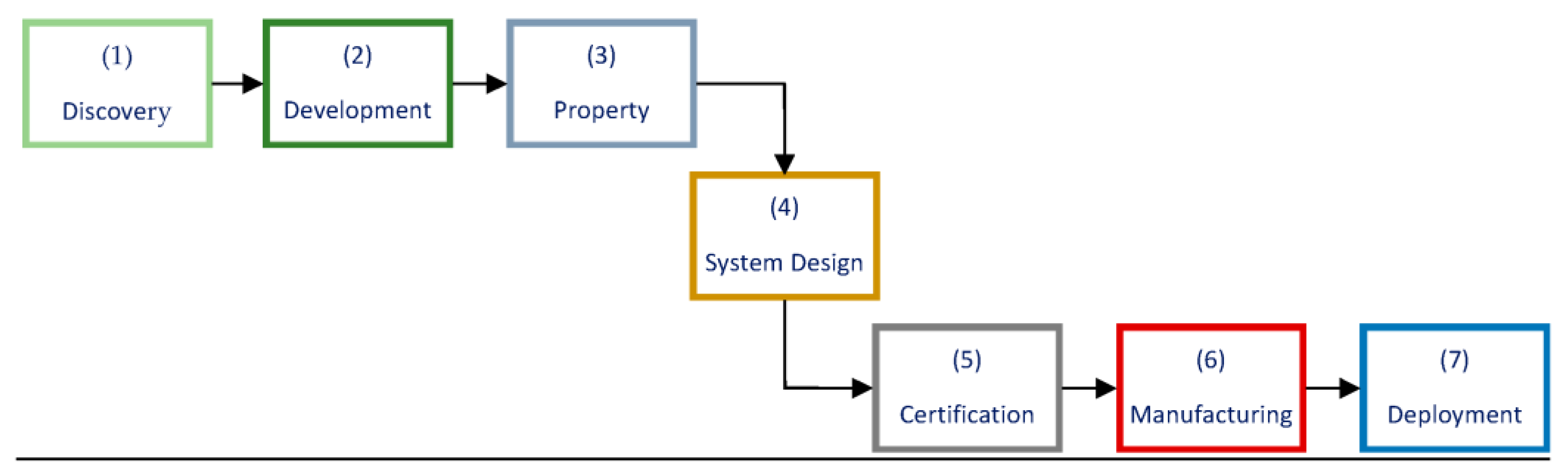
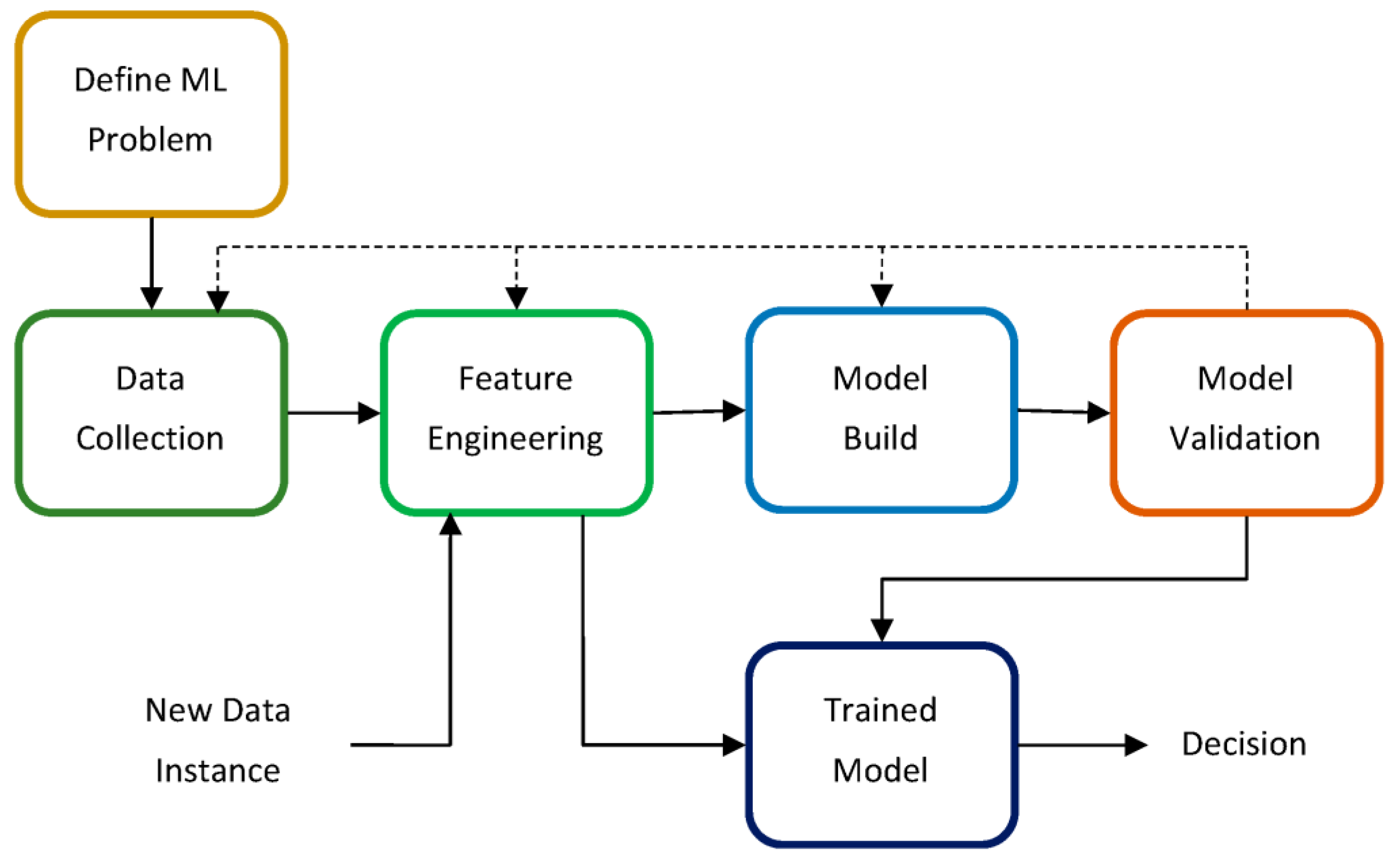
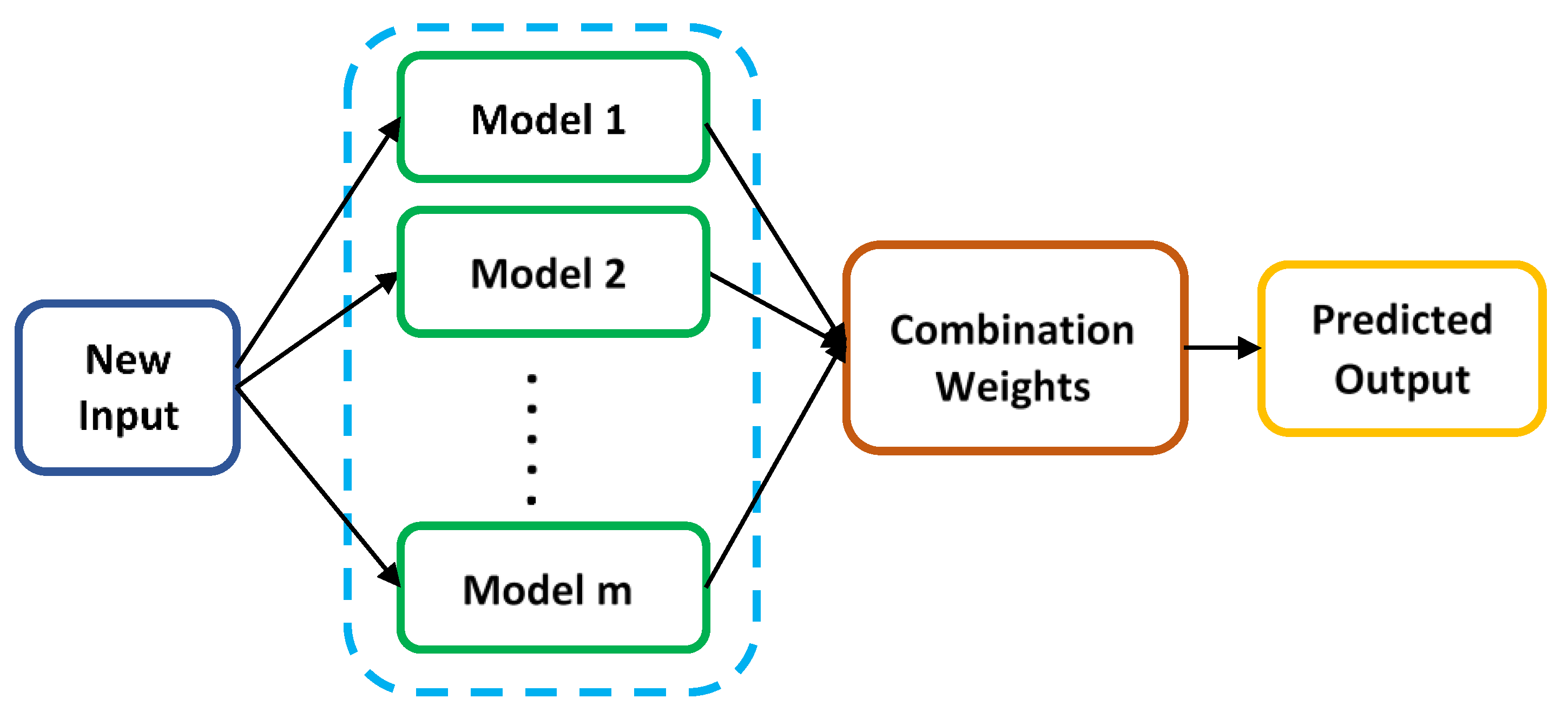
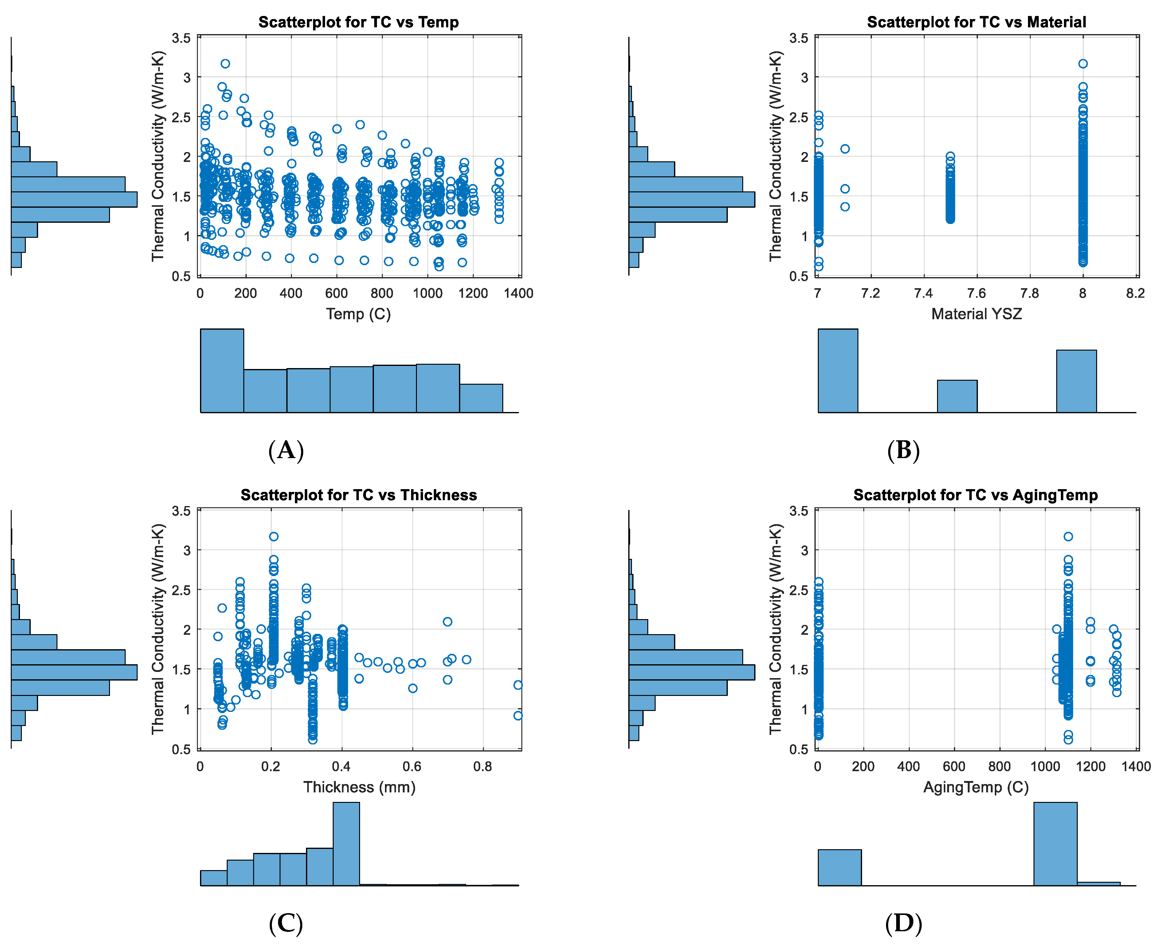
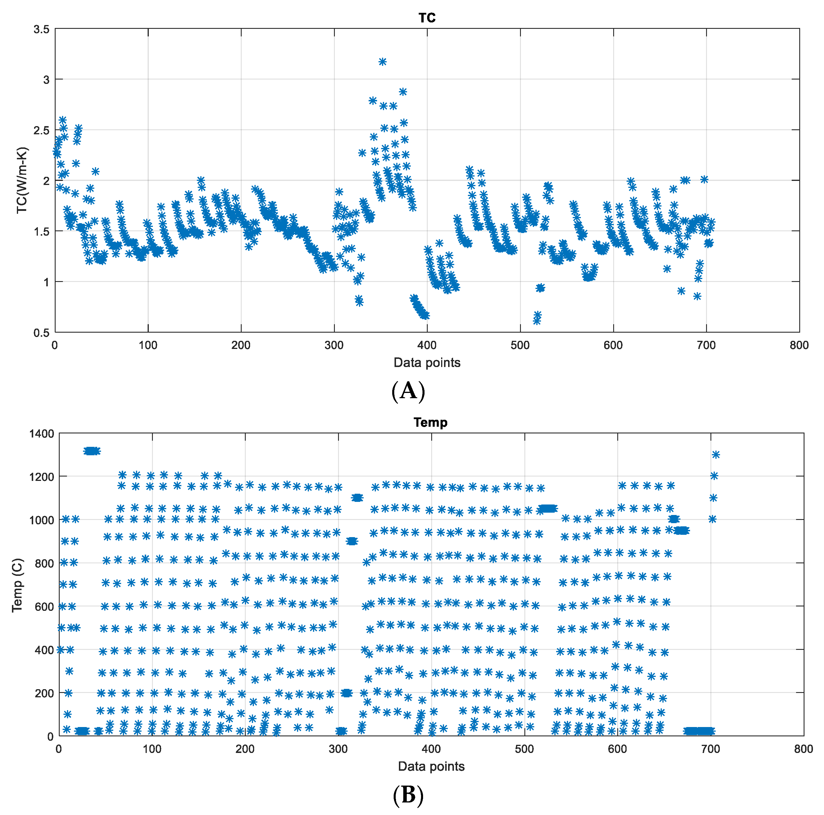
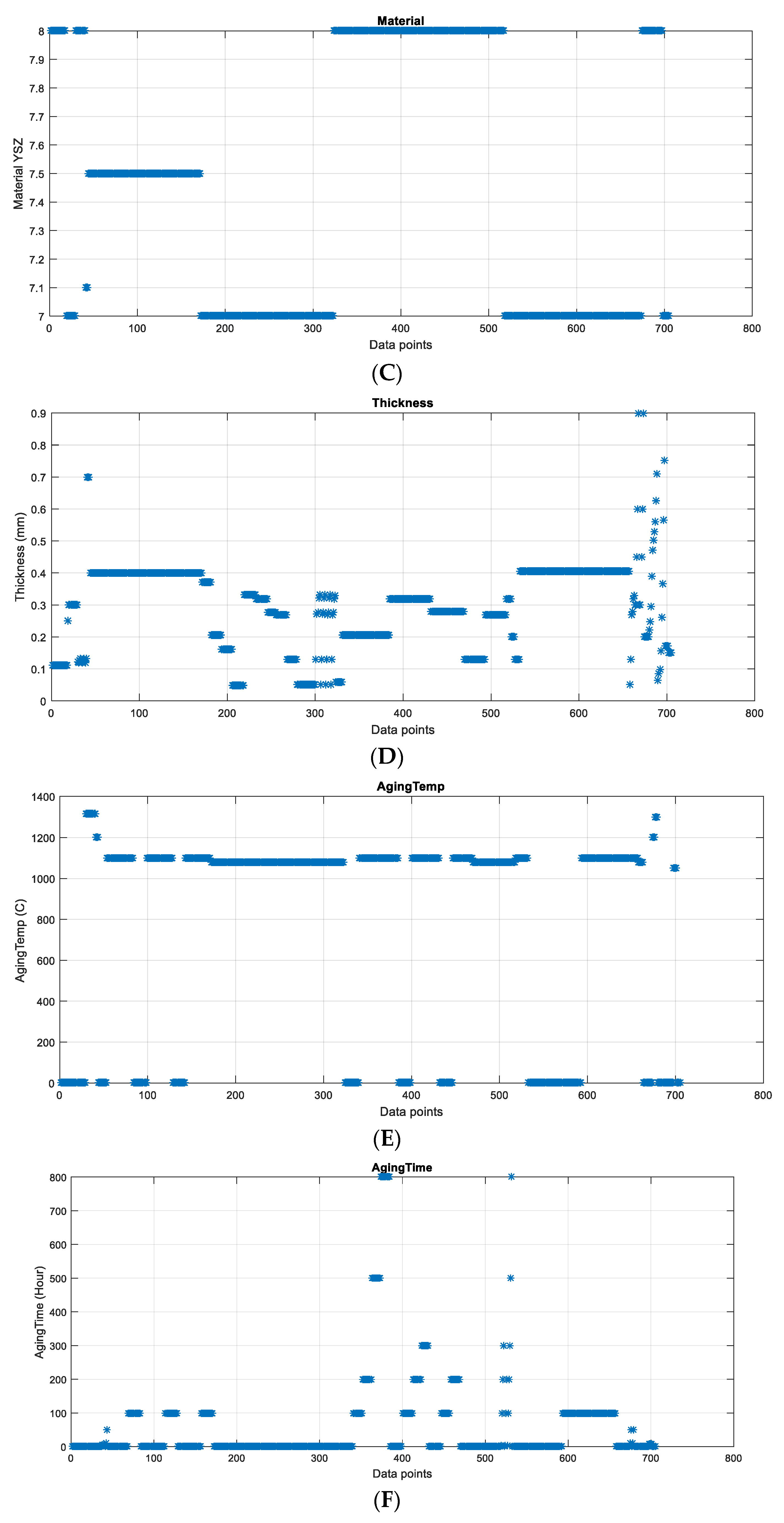
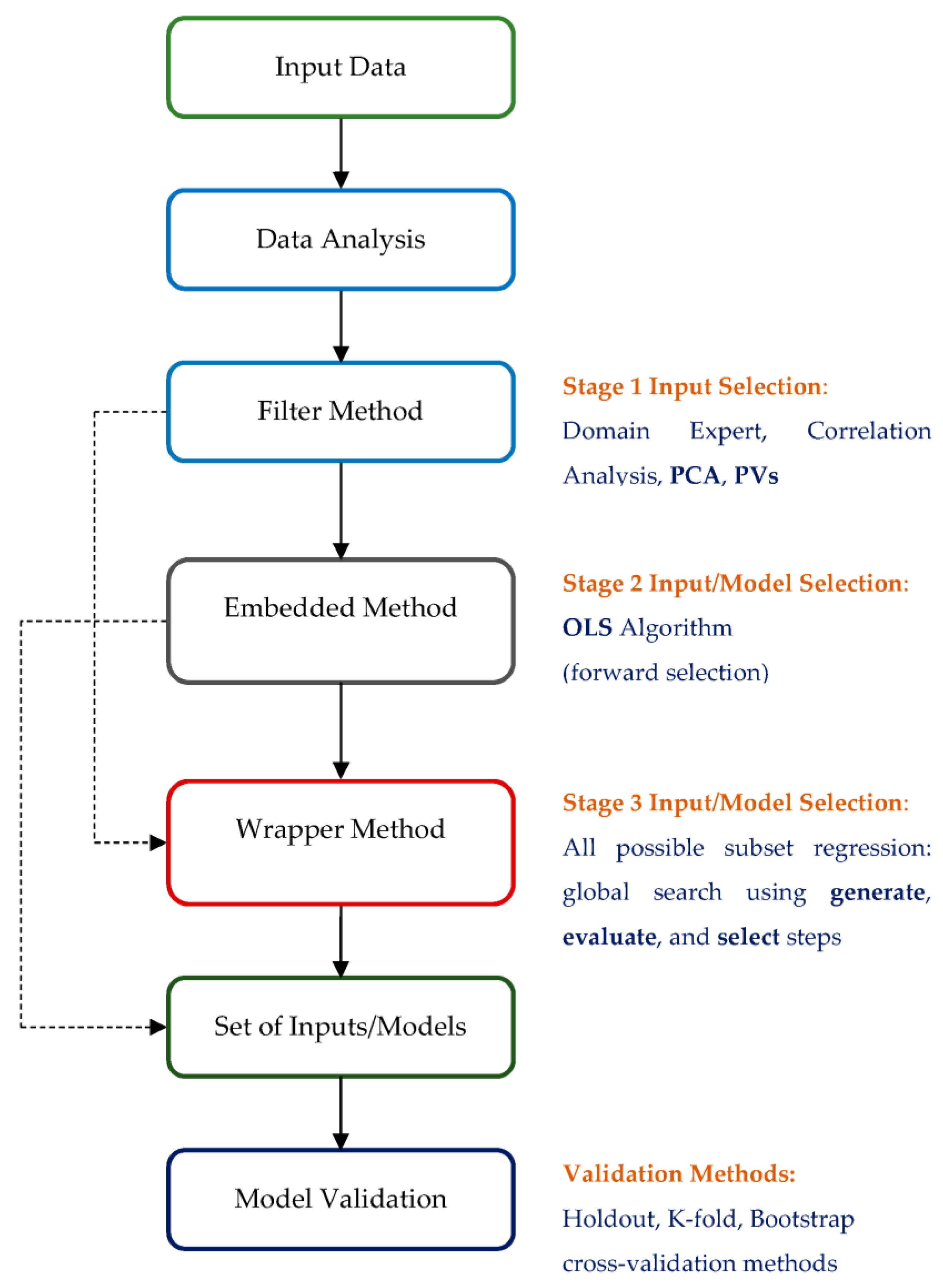
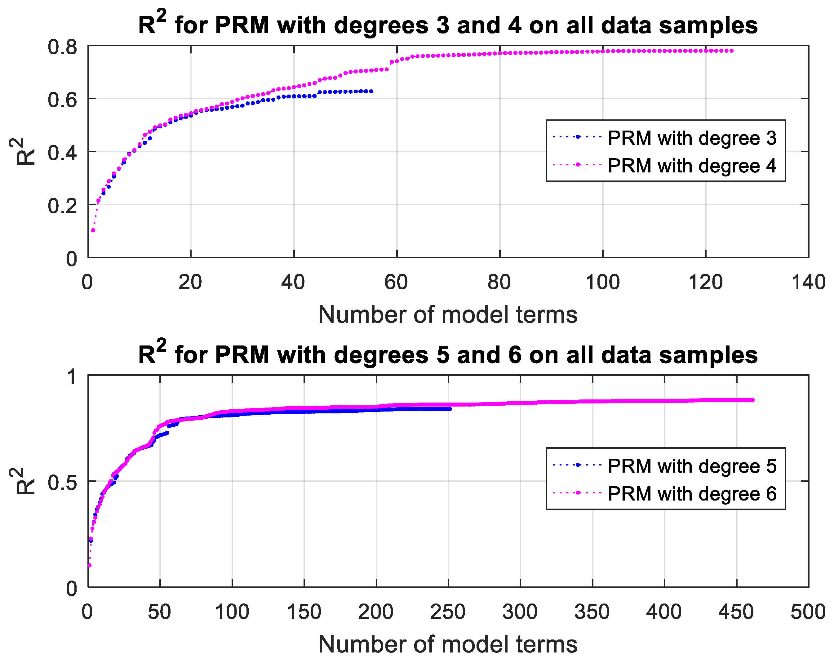
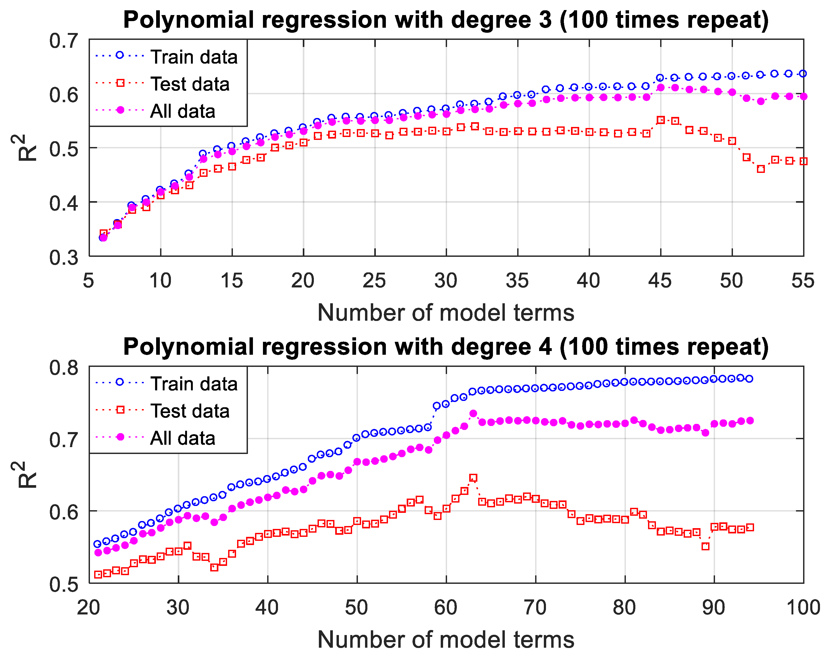
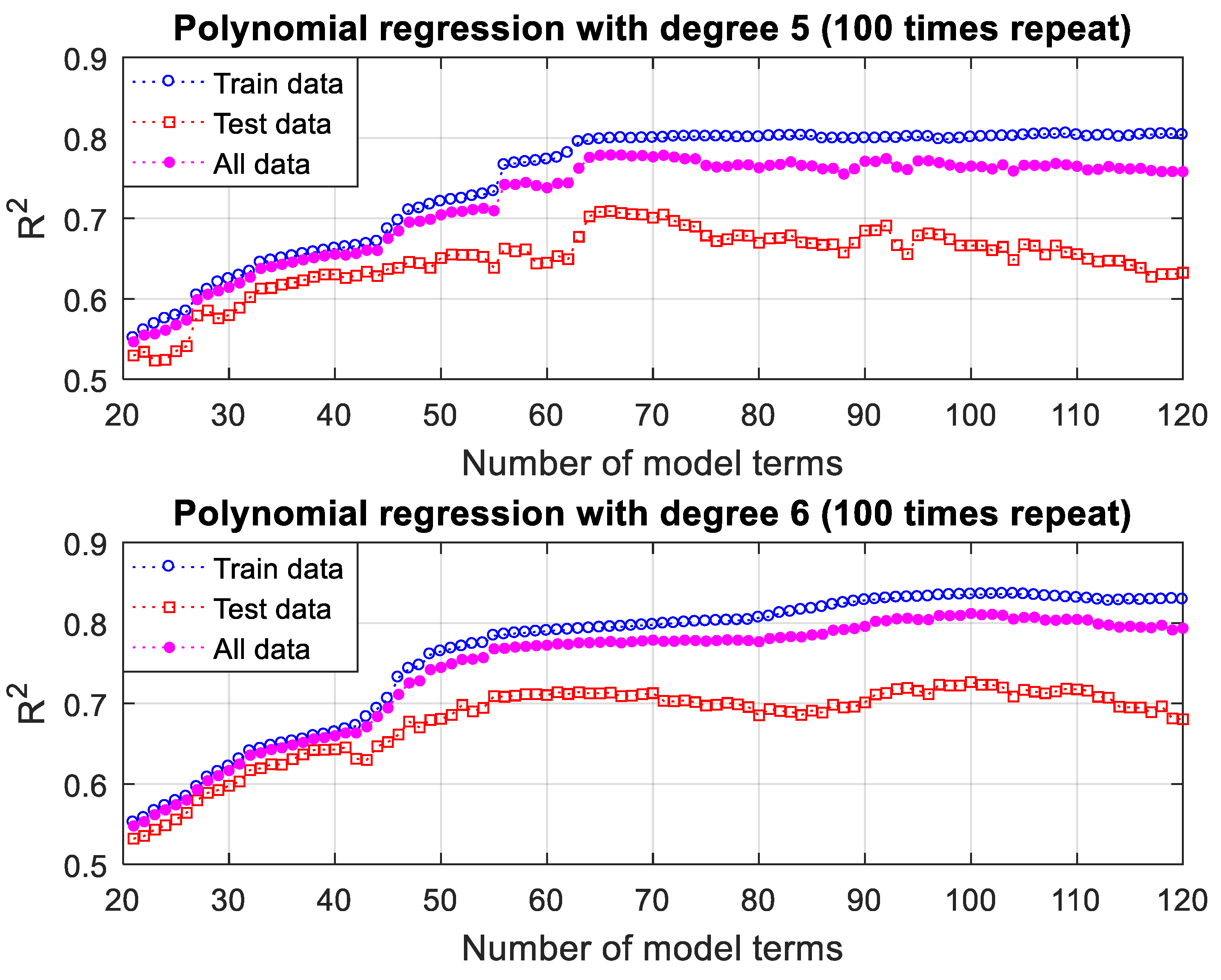
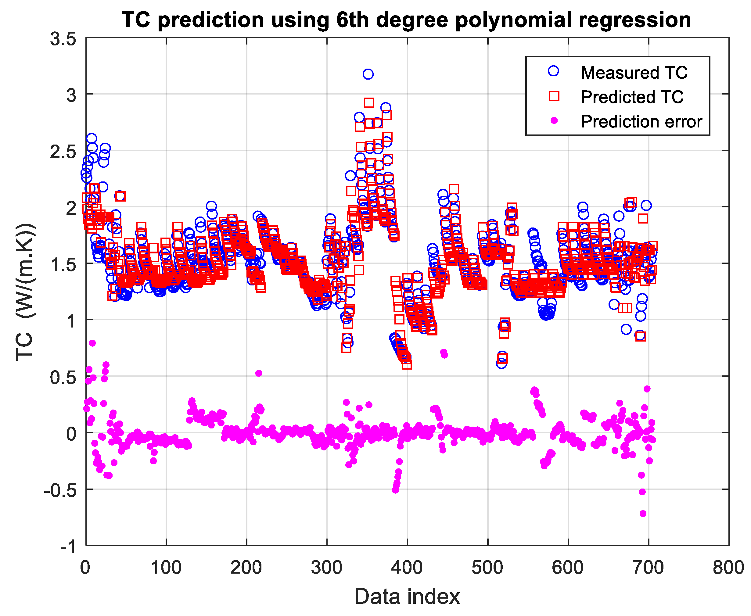
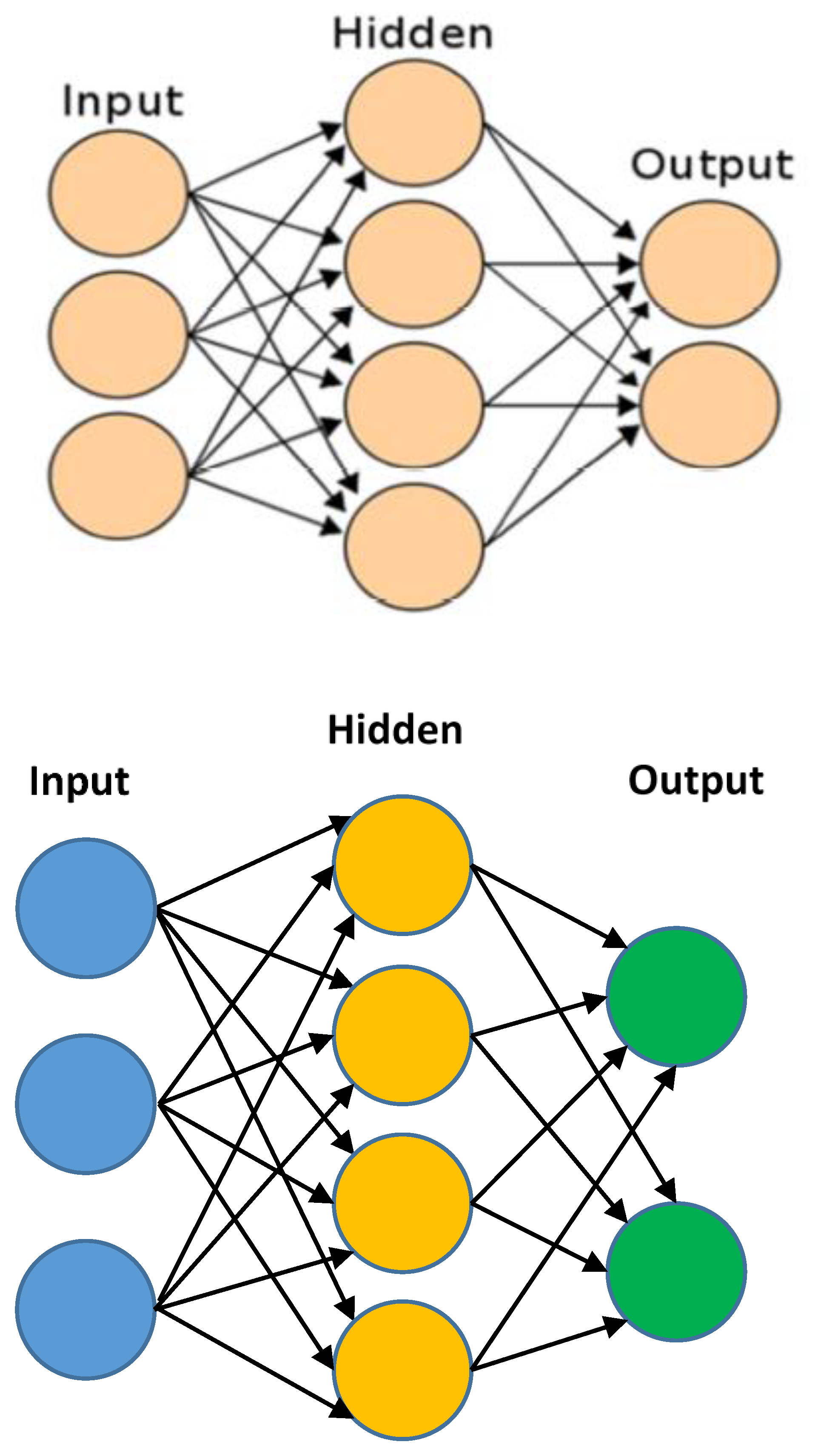
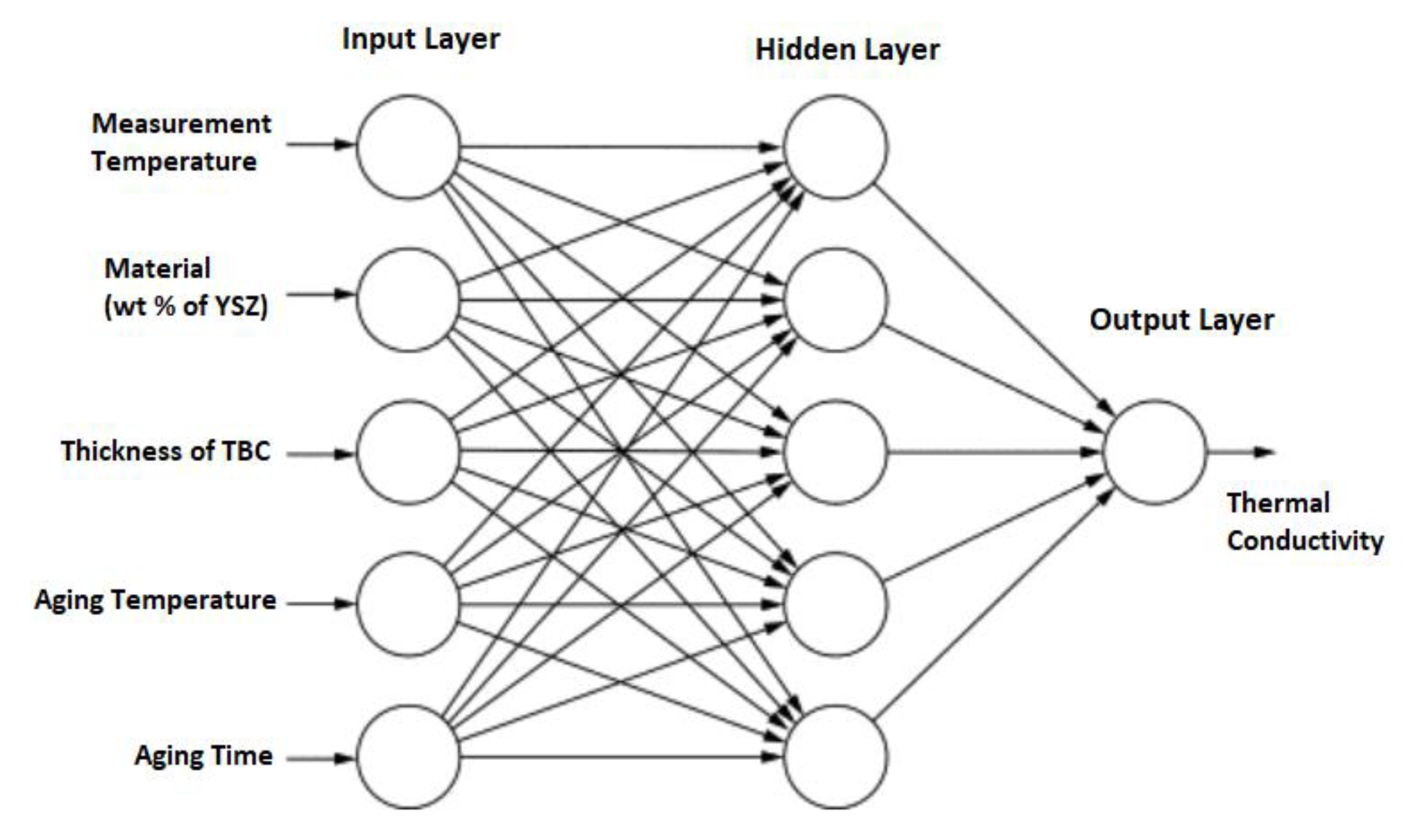
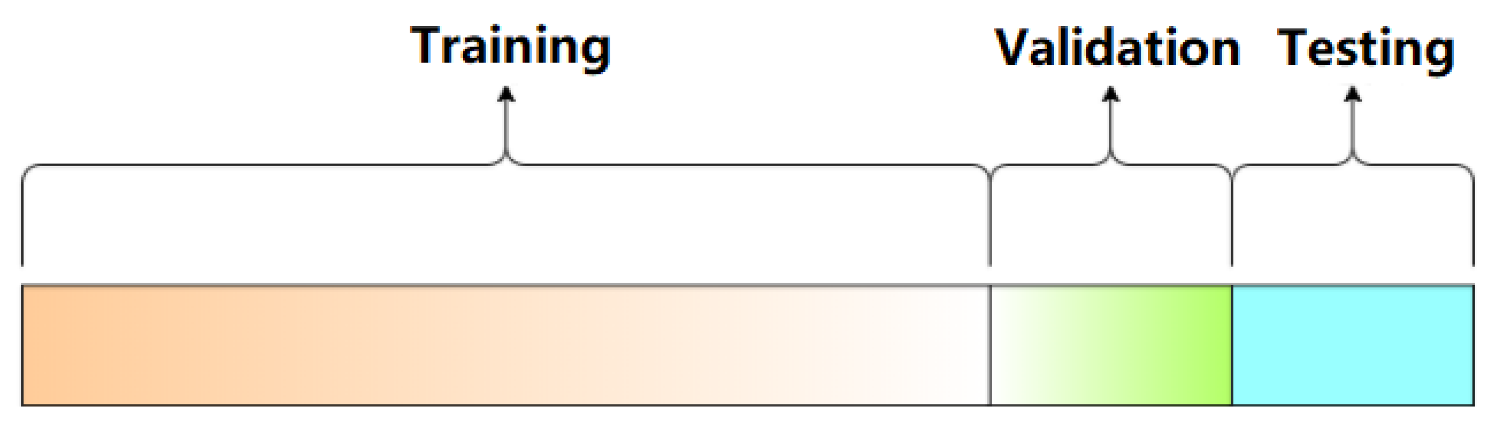
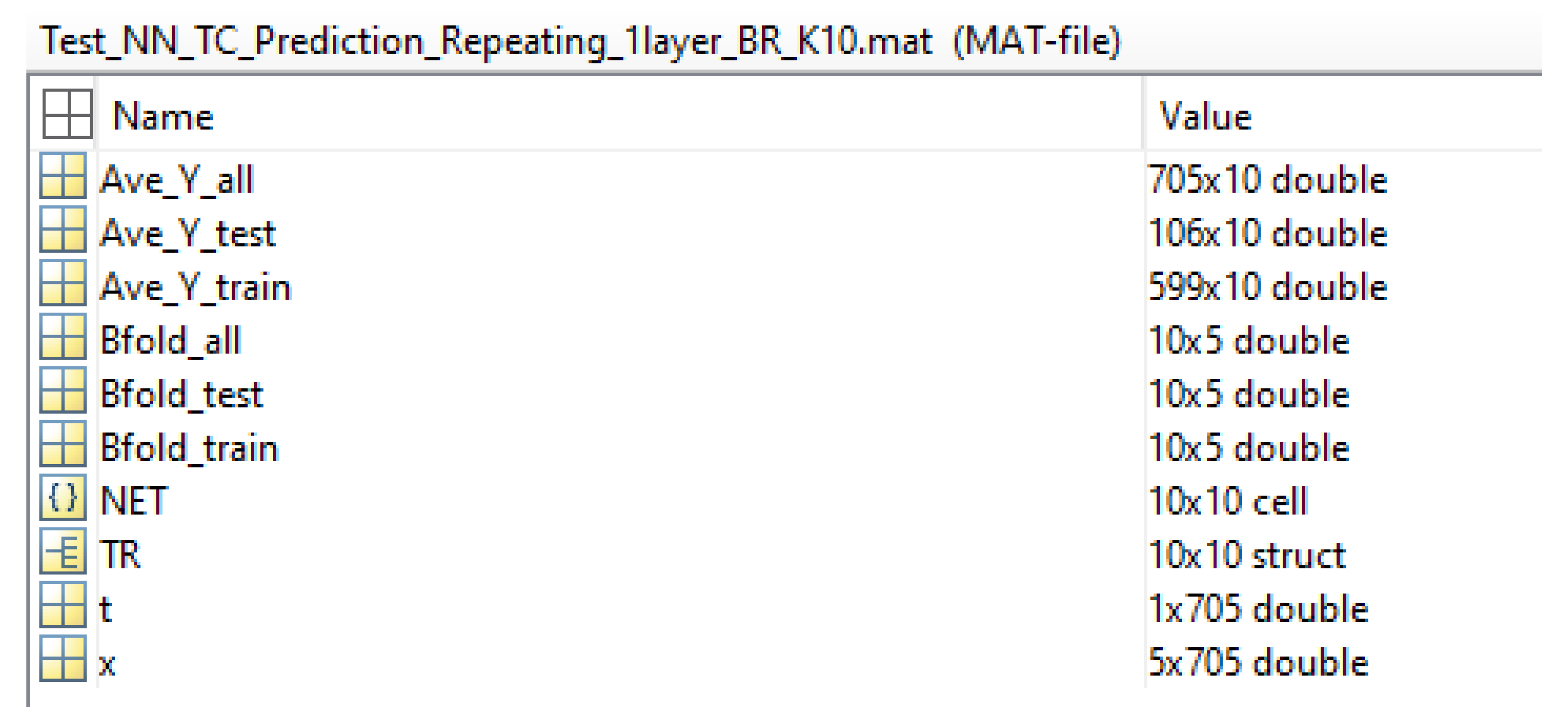
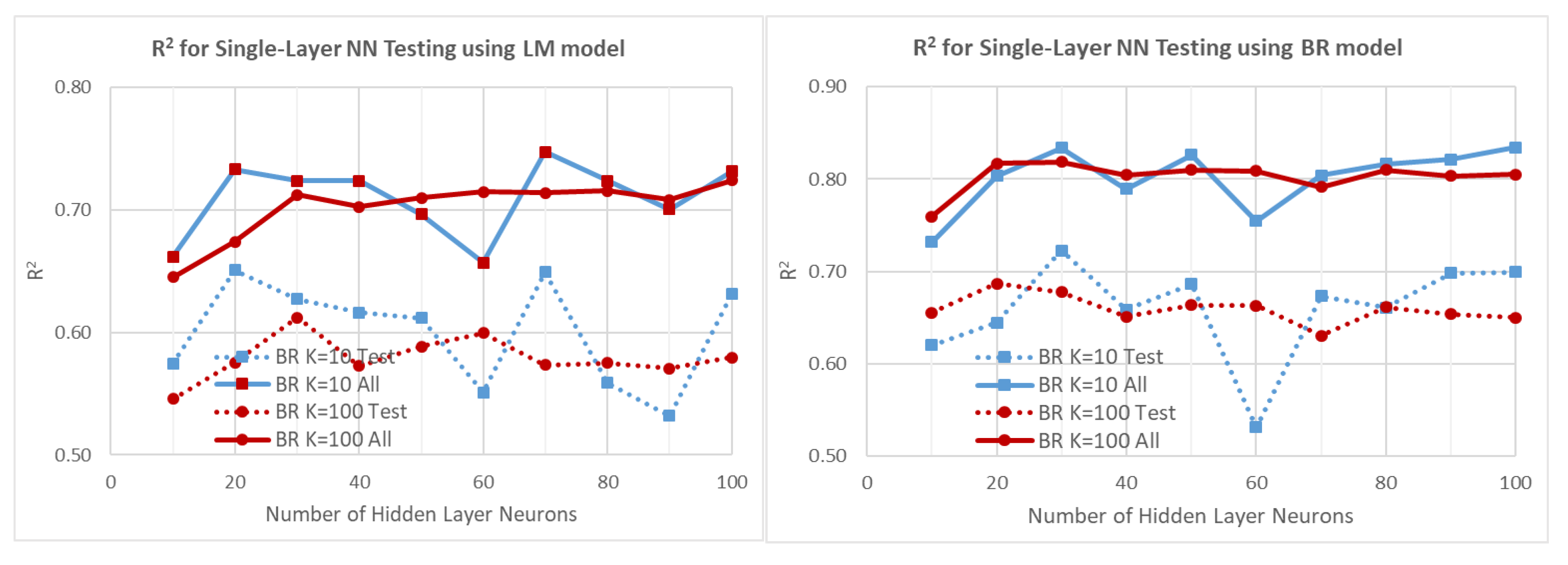
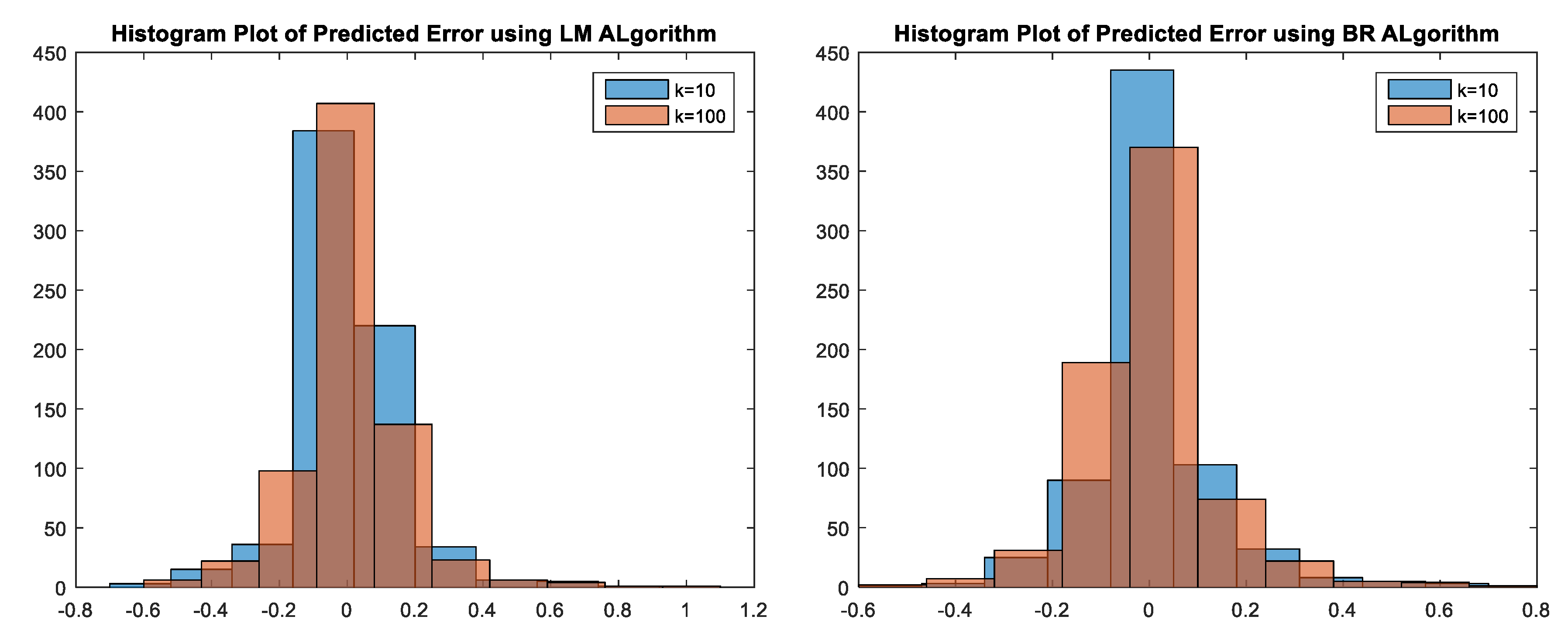
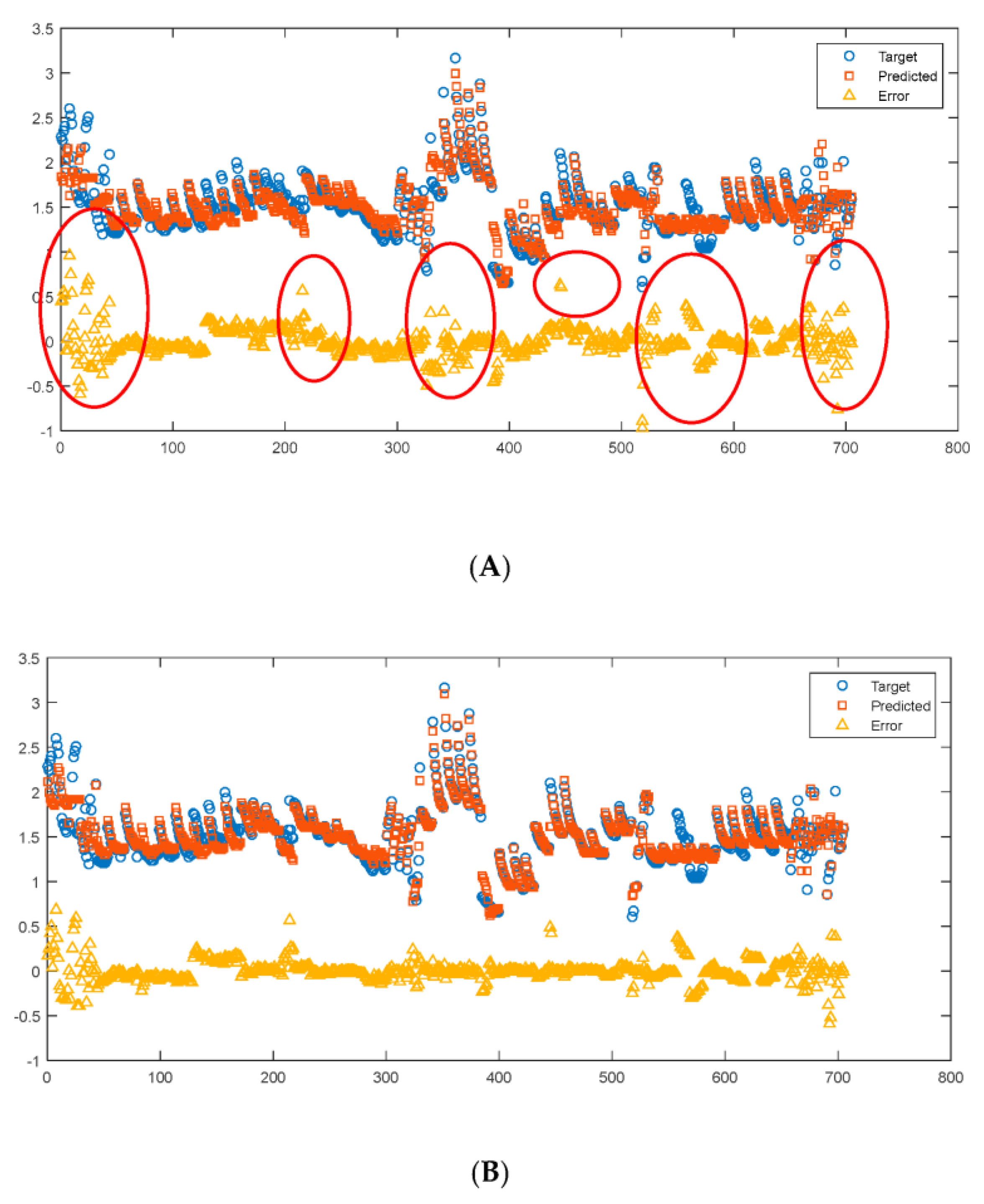
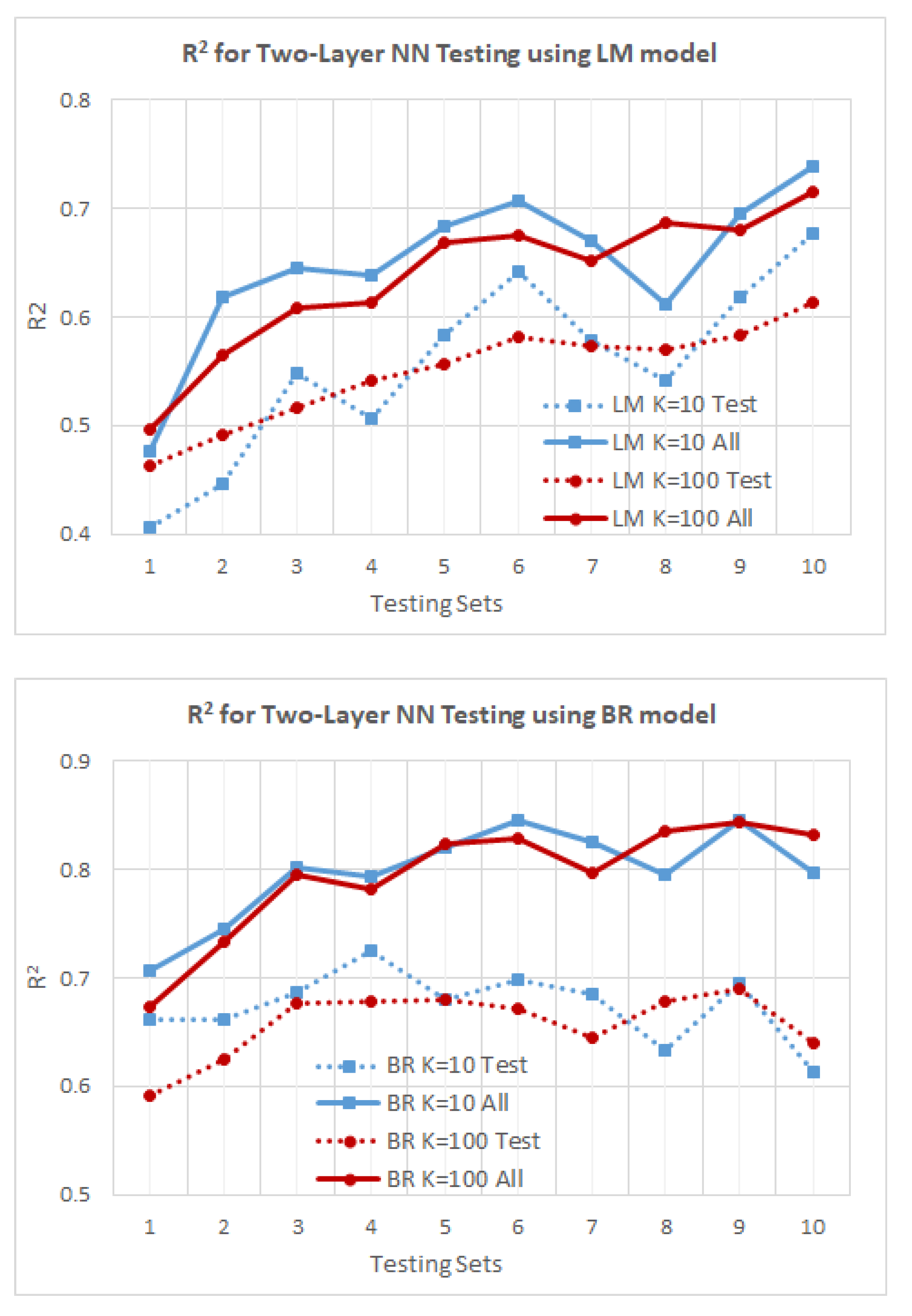
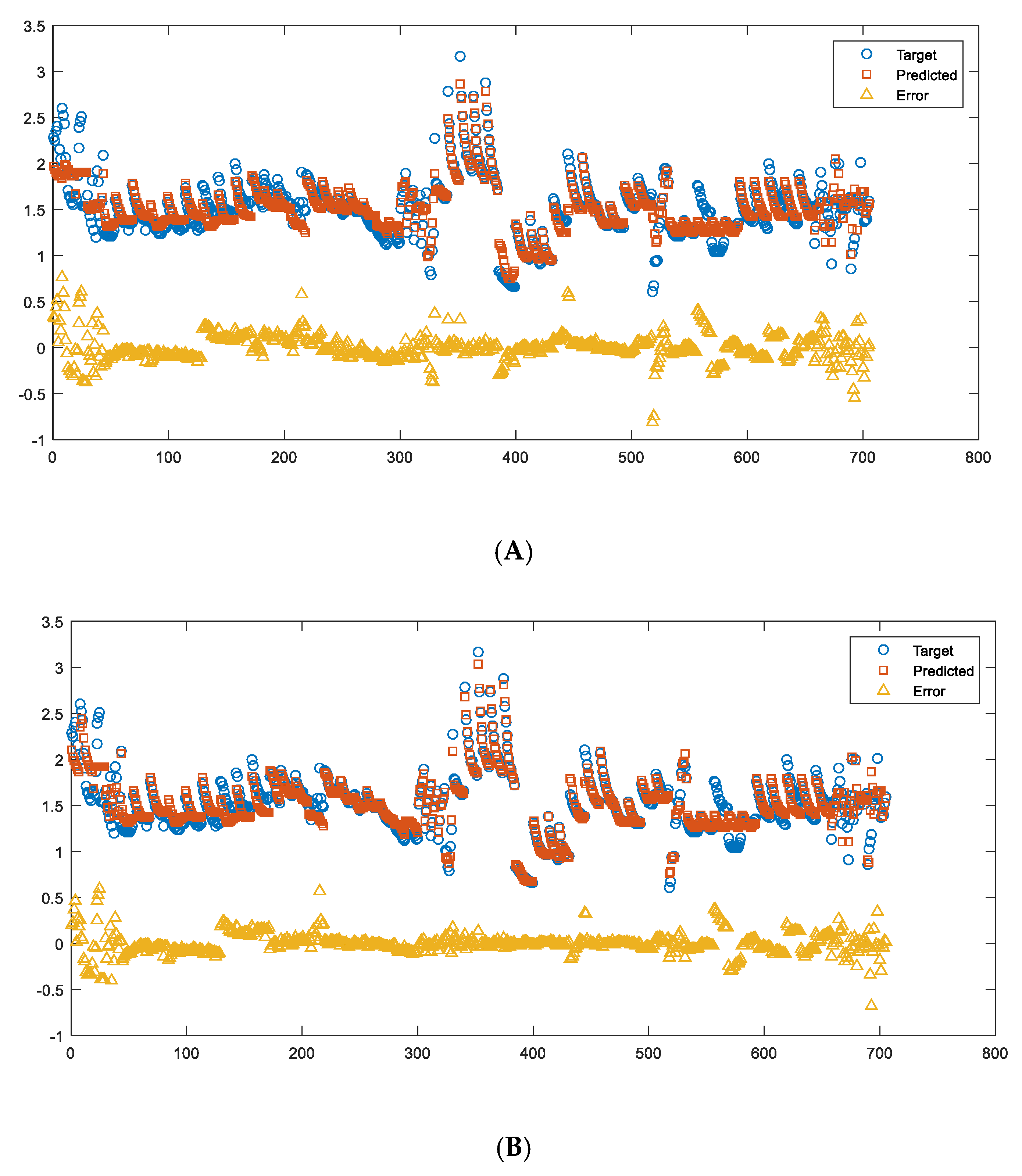
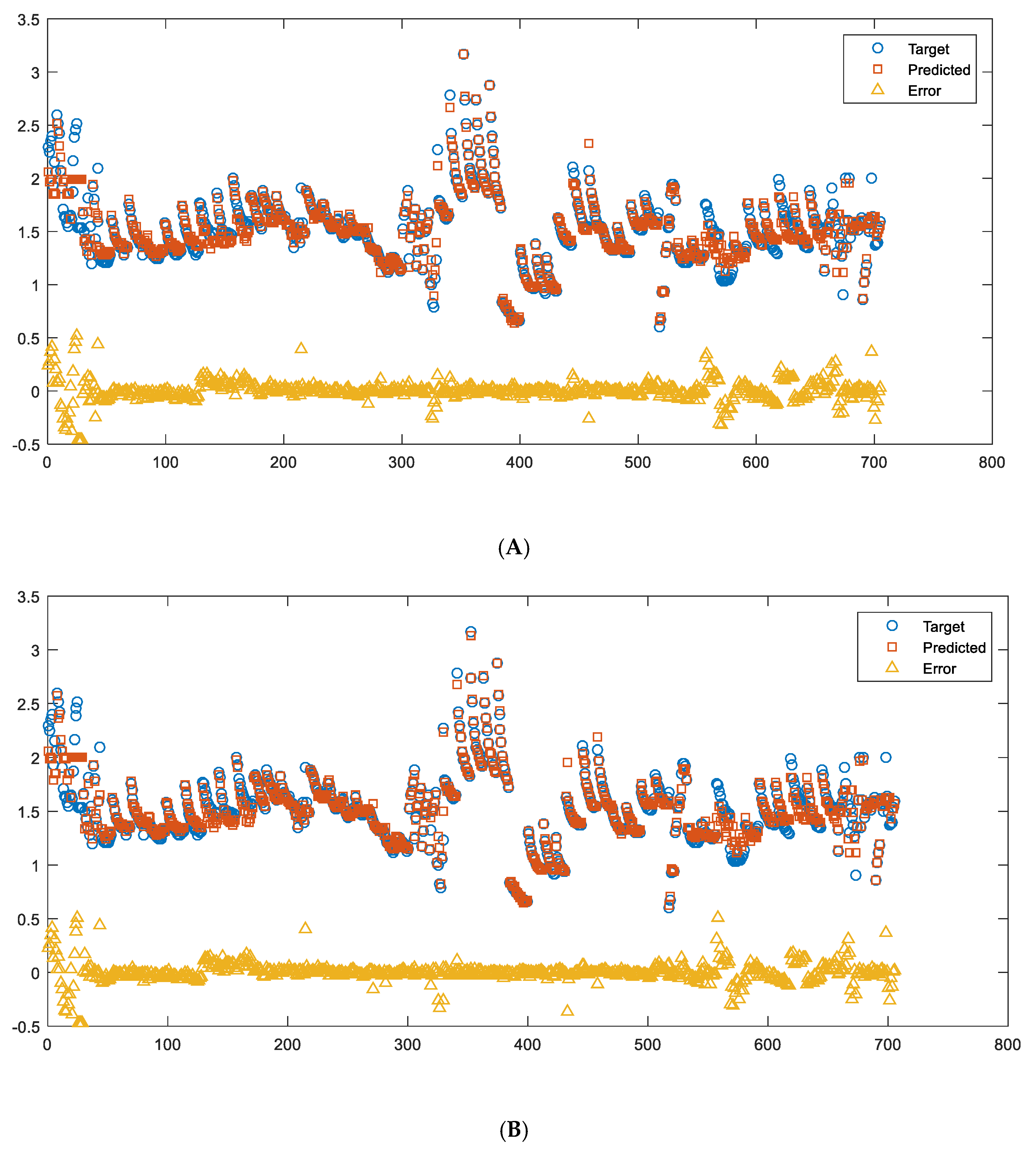
Table A1. List of some of the publicly available materials databases.

Name and Category	Website and References	Description
AFLOWLIB Computational	aflowlib.org [118]	Online computational platform for determining thermodynamic stability, electronic band structures, vibrational dispersions and thermomechanical properties of various inorganic compounds.
Computational Materials Repository Computational	cmr.fysik.dtu.dk [114]	Material database system supporting a variety of tools for collecting, storing, grouping, searching, retrieving and analyzing electronic structure calculations generated by many modern electronic-structure simulators.
Crystallography open database Crystallography	crystallography.net [119]	Online database that provides information on a variety of known atomic coordinates of crystal structures of organic, inorganic, metal-organic compounds and minerals collected from several research publications.
MARVEL NCCR Computational	nccr-marvel.ch [120]	Material informatics platform focusing on the design and discovery of new materials via data driven, high performance quantum mechanical simulations. Research tools, computational data and simulation software accessible through the materials cloud platform.
Materials Project Computational	materialsproject.org [121]	Online platform that provides access to density functional theory (DFT) calculations on a large number of metallic compounds, energy materials and also mechanical properties of many materials.
MatNavi(NIMS) General Materials data	mits.nims.go.jp/ index_en.html [122]	Integrated material database system comprising structures and properties for various materials including polymers and inorganic substances.
Organic materials database Computational	omdb.mathub.io [123]	Electronic structure database of three-dimensional organic crystals that also provides tools for search queries.
Open quantum materials database Computational	oqmd.org [124]	A high throughput database comprising the thermodynamic and structural properties of the known crystalline solids which are calculated using the density functional theory computation technique.
Open materials database Computational	openmaterialsdb.se [125]	A high throughput computational database which is based on structures from the Crystallography open database and provides information on the properties of various materials.
SUNCAT/CatApp Catalysts	suncat.stanford.edu/catapp [126]	Materials informatics center focusing on catalyst and materials design for next-generation energy solutions. Computational results for thousands of surface reactions and online tools accessible at catalysis-hub.org.
Chemspider Chemical data	chemspider.com [127]	Chemical structure database containing information on physio-chemical properties, interactive spectra, links to chemical vendor’s catalogs, literature references and patents collected from a wide range of data sources.
Citrination General Materials Data	citrination.com [128]	Materials informatics platform containing information on the computed and experimental properties of various materials and chemicals.
NIST Materials Data Repository (DSpace) General Materials Data	materialsdata.nist.gov/dspace/xmlui [129]	File repository that accepts materials data in any format related to specific research publications. The repository is implemented using a technology called Dspace.
NanoHUB Nanomaterials	nanohub.org [130]	Premier online resource that offers course materials, lectures, seminars, tutorials, professional networking and interactive simulation tools for nanotechnology.
Nanomaterials Registry Nanomaterials	nanomaterialregistry.org [131]	A central web-based repository that provides links to associated journals and publications, interactive simulation tools, computational results and information such as physio-chemical characteristics, and biological and environmental study data for different nanomaterials.
NIST Interatomic Potentials Repository Computational	ctcms.nist.gov/potentials [132]	A reliable source for interatomic potentials and related files for various metals. Evaluation tools to help researchers judge the quality and applicability of their interatomic models are also available.
PubChem Chemical data	pubchem.ncbi.nlm.nih.gov [133]	A database that contains information on chemical substances and their biological activities.
TEDesignLab Thermoelectrics	tedesignlab.org [134]	A virtual platform that contains raw experimental and computational thermoelectric data and a suite of interactive web-based tools that help in the design of new thermoelectric material.
UCSB-MRL thermoelectric database Thermoelectrics	mrl.ucsb.edu:8080/datamine/thermoelectric.jsp [135]	A large repository created by extracting thermoelectric materials data from several publications.

Table A2. List of some of the commercially available materials databases.

Name and Category	Website and References	Description
Inorganic Crystal Structure Database Crystallography	cds.dl.ac.uk/cds/datasets/ crys/icsd/llicsd.html [136]	Repository providing information of various inorganic crystal structures.
Cambridge Crystallographic Data Centre Crystallography	ccdc.cam.ac.uk/pages/Home.aspx [137]	Non-profit organization that compiles and maintains the Cambridge Structural Database, which contains information of various organic and metal organic small molecule crystal structures.
NIST Standard Reference Data General Materials Data	nist.gov/srd/dblistpcdatabases.cfm [138]	Generic material property data that provides measurable quantitative information related to physical, chemical or biological properties of known substances.
CALPHAD databases (e.g., Thermocalc SGTE) Thermodynamics	thermocalc.com/products-services/ databases/thermodynamic [139]	Journal publishing the experimental and theoretical information on phase equilibria and thermochemical properties of various materials.
ASM Alloy Center Database Alloys	mio.asminternational.org/ac [140]	Database for researching accurate materials data of compositions, properties, performance details and processing guidelines from authoritative sources for specific metals and alloys.
ASM Phase Diagrams Thermodynamics	asminternational.org/AsmEnterprise/APD [141]	Online repository that provides information related to binary and ternary alloy phase diagrams and associated crystal data for many alloy systems.
MatDat General Materials Data	matdat.com [142]	Online database that provides information on published design-relevant material data to the industrial, academic and research community.
Pauling File General Materials Data	paulingfile.com [143]	Online database that includes information on the crystal structures, physical properties and phase diagrams for various non-organic solid-state materials.
Springer Materials General Materials Data	materials.springer.com [144]	Materials research platform that provides curated data for identifying material properties and a set of advanced functionalities for data analysis and visualization of materials properties.
Total Materia General Materials Data	totalmateria.com [145]	Online materials database that includes search and cross-reference tools, chemical composition, properties and specifications for various metals, polymers, ceramics and composites.

Table A3. Summarized experimental researf105ches on TC of TBC.

	Year	Author	Material	Research Topic
1	1998	Taylor [146]	Al₂O₃ and ZrO₂ and of four and eight alternating layers of Al₂O₃–ZrO₂	TC vs. temp and different thickness
2	1998	Raghavan [147]	5.8 wt.% yttria YSZ	TC vs. temp and densities (% of theoretical) and grain diameters (in nm)
3	1999	An [86]	Al₂O₃ and 8YSZ	TC vs. temp
4	2000	Zhu [148]	EB-PVD. ZrO2-8 wt.%Y₂O₃ (8YSZ)	TC vs. time for different thickness
5	2002	Nicholls [87]	EB-PVD TBCs 7YSZ	TC vs. Yttia (wt%), TC vs. T and grain size; thermal conductivities of dopant modified EB-PVD TBCs at 4 mol% addition and 250 mm thickness; data measured at room temperature
6	2002	Zhu [149]	YSZ-Nd-Yb and YSZ-Gd-Yb; 8YSZ	TC vs. temp and time; TC vs. total dopant concentration
7	2004	Cernuschi [150]	8Y₂O₃ZrO₂, 22 wt.%MgO–ZrO₂, and 25 wt.%CeO₂–2.5Y₂O₃–ZrO₂	TC vs. temp for different cycles
8	2004	Jang [88]	EB-PVD ZrO₂-4 mol% Y₂O₃	TC vs. substrate thickness (areal thermal diffusion time)
9	2004	Singh [89]	EB-PVD 8YSZ, ZrO₂–8% Y₂O₃ HfO₂-40% wtZrO₂-27 wt%Y₂O₃	TC vs. time and number of layers
10	2004	Matsumoto [90]	ZrO₂–Y₂O₃–La₂O₃	TC vs. La₂O₃ content %
11	2005	Wolfe [151]	ZrO₂– 8 wt.% Y₂O₃	TC vs. time and number of layers
12	2006	Renteria [76]	three morphologically different EB-PVD PYSZ TBC	TC vs. temp and time
13	2006	Rätzer-Scheibe [91]	EB-PVD PYSZ	TC vs. temp and thickness
14	2006	Ma [152]	SPPS-7YSZ and SPPS LK-Zr	TC vs. temp and time
15	2007	Almeida [92]	EB-PVD 2O₃–ZrO₂	TC vs. temp
16	2007	Rätzer-Scheibe [84]	EB-PVD ZrO₂–7wt.%Y₂O₃	TC vs. temp and heat treatment time and thickness
17	2007	Schulz [93]	EB-PVD (Three types) FeCrAlY; PYSZ	TC vs. temp; aging time
18	2008	Jang [94]	EB-PVD ZrO₂–4 mol% Y₂O₃	TC vs. number of layers, porosity
19	2009	Matsumoto [95]	EB-PVD YSZ, La₂O₃ and HfO₂	TC vs. annealing time
20	2010	Yu [153]	plasma sprayed Sm₂Zr₂O₇	TC vs. temp and different heat-treating temperature
21	2011	Jang [96]	EB-PVD ZrO₂–4 mol% Y₂O₃	TC vs. coating thickness
22	2011	Liu [97]	EB-PVD 7wt% Y₂O₃ (7YSZ)	TC vs. substrate rotation speed
23	2012	Limarga [154]	EB-PVD 3wt% Y₂O₃ (3YSZ)	TC vs. temp and different heat-treating temperature and time
24	2012	Łatka [155]	ZrO₂+8 wt.%Y₂O₃ (8YSZ)	TC vs. temp
25	2012	Zhang [156]	(La_0.95Mg_0.05)2Ce₂O_6.95 (La_0.95Mg_0.05)2Ce₂O_6.95 La₂Ce₂O₇	TC vs. temp
26	2013	Jang [157]	ZrO₂–4 mol.%Y₂O₃ (TZ4Y)	TC vs. temp and different sintered temp and different GD₂O₃ percentile
27	2013	Bobzin [98]	EB–PVD 7YSZ, La₂Zr₂O₇, 7YSZ + Gd₂Zr₂O₇ DCL, Gd₂Zr₂O₇, 7YSZ + Gd₂Zr₂O₇	TC vs. temp
28	2013	Sun [158]	Yb₂O₃–Y₂O₃–ZrO₂	TC vs. temp
29	2013	Zhao [159]	EB-PVD ZrO₂ Y₂O₃ (8YSZ), 4TiYSZ, to 16TiYSZ	TC vs. temp
30	2014	Jordan [160]	SPPS YSZ TBCs with IPBs	TC for different trials
31	2014	Lu [161]	LSMZATO, La_1−xSr_xMg_1−xZn_xAl₁₁ xTixO₁₉	TC vs. temp
32	2014	Wang [162]	YSZ/NiCoCrAlY	TC vs. temp (numerical)
33	2015	Rai [163]	YSZ and GZO	TC for different layer and thickness
34	2016	Guo [164]	1RE₁Yb–YSZ 1La₁Yb–YSZ	TC vs. temp
35	2016	Arai [165]	YSZ (0, 5, 10, 15 wt%)	TC vs. porosity, width of pore, at 570 K
36	2016	Guo [166]	La₂Zr₂O₇	TC vs. temp
37	2016	Wang [167]	8YSZ	Numerical work (mathematic model) TC vs. porosity and pores size
38	2016	Zhang [168]	La₂(Ce_0.3Zr_0.7)₂O₇-3 wt.%Y₂O₃	TC vs. temp (deposited at 5, 15 and 25 RPM)
39	2017	Meng [169]	(a) La₂Zr₂O₇; (b) Nd₂Zr₂O₇; (c) Sm₂Zr₂O₇; (d) Gd₂Zr₂O₇.	TC vs. temp, concentration increase in oxygen vacancies

References

Reyes, K.G.; Maruyama, B.; Editors, G. The machine learning revolution in materials? MRS Bull. 2019, 44, 530–537. [Google Scholar] [CrossRef] [Green Version]
Himanen, L.; Geurts, A.; Foster, A.S.; Rinke, P. Data-Driven Materials Science: Status, Challenges, and Perspectives. Adv. Sci. 2019, 6, 1900808. [Google Scholar] [CrossRef] [PubMed]
Wei, J.; Chu, X.; Sun, X.Y.; Xu, K.; Deng, H.X.; Chen, J.; Wei, Z.; Lei, M. Machine learning in materials science. InfoMat 2019, 1, 338–358. [Google Scholar] [CrossRef] [Green Version]
Liu, Y.; Zhao, T.; Ju, W.; Shi, S. Materials discovery and design using machine learning. J. Mater. 2017, 3, 159–177. [Google Scholar] [CrossRef]
Agrawal, A.; Choudhary, A. Perspective: Materials informatics and big data: Realization of the “fourth paradigm” of science in materials science. APL Mater. 2016, 4, 053208. [Google Scholar] [CrossRef] [Green Version]
Zhou, T.; Song, Z.; Sundmacher, K. Big Data Creates New Opportunities for Materials Research: A Review on Methods and Applications of Machine Learning for Materials Design. Engineering 2019, 5, 1017–1026. [Google Scholar] [CrossRef]
Pokluda, J.; Kianicová, M. Damage and Performance Assessment of Protective Coatings on Turbine Blades. In Gas Turbines, 1st ed.; SCIYO, 2010; pp. 283–306. Available online: https://www.intechopen.com/chapters/12092 (accessed on 10 March 2023).
Vaßen, R.; Jarligo, M.O.; Steinke, T.; Mack, D.E.; Stöver, D. Overview on advanced thermal barrier coatings. Surf. Coat. Technol. 2010, 205, 938–942. [Google Scholar] [CrossRef]
Warren, J.A. The Materials Genome Initiative and artificial intelligence. MRS Bull. 2018, 43, 452–457. [Google Scholar] [CrossRef]
Hautier, G.; Jain, A.; Ong, S.P. From the computer to the laboratory: Materials From the computer to the laboratory: Materials discovery and design using first-principles calculations. J. Mater. Sci. 2012, 47, 7317–7340. [Google Scholar] [CrossRef] [Green Version]
Jose, R.; Ramakrishna, S. Materials 4.0: Materials big data enabled materials discovery. Appl. Mater. Today 2018, 10, 127–132. [Google Scholar] [CrossRef]
National Science and Technology Council. Materials Genome Initiative for Global Competitiveness; Aeromat 23 Conference and Exposition American Society for Metals; American Society for Metals: Charlotte, NC, USA, 2012. [Google Scholar]
Mueller, T.; Kusne, G.K.; Ramprasad, R. Machine learning in materials science: Recent progress and emerging applications. In Reviews in Computational Chemistry; John Wiley & Sons, Inc.: Hoboken, NJ, USA, 2016. [Google Scholar]
Aartsen, M.G.; Ackermann, M.; Adams, J.; Aguilar, J.A.; Ahlers, M.; Ahrens, M.; Altmann, D.; Anderson, T.; Arguelles, C.; Arlen, T.C.; et al. Determining neutrino oscillation parameters from atmospheric muon neutrino disappearance with three years of IceCube DeepCore data. Phys. Rev. D-Part. Fields Gravit. Cosmol. 2015, 91, 072004. [Google Scholar] [CrossRef] [Green Version]
Kalidindi, S.R.; Medford, A.J.; McDowell, D.L. Vision for Data and Informatics in the Future Materials Innovation Ecosystem. JOM 2016, 68, 2126–2137. [Google Scholar] [CrossRef]
Hill, J.; Mulholland, G.; Persson, K.; Seshadri, R.; Wolverton, C.; Meredig, B. Materials science with large-scale data and informatics: Unlocking new opportunities. MRS Bull. 2016, 41, 399–409. [Google Scholar] [CrossRef] [Green Version]
Ravichandran, T.; Liu, Y.; Kumar, A.; Srivastava, A.; Hanachi, H.; Heppler, G. Data-Driven Performance Prediction Using Gas Turbine Sensory Signals. In Proceedings of the 2020 IEEE Canadian Conference on Electrical and Computer Engineering (CCECE), London, ON, Canada, 30 August–2 September 2020. [Google Scholar] [CrossRef]
Bishop, C.M. Pattern Recognition and Machine Learning; Springer: Berlin/Heidelberg, Germany, 2006. [Google Scholar]
Hastie, T.; Tibshirani, R.; Friedman, J. The Elements of Statistical Learning: Data Mining, Inference, and Prediction; Springer: New York, NY, USA, 2009. [Google Scholar]
Nigsch, F.; Bender, A.; van Buuren, B.; Tissen, J.; Nigsch, E.; Mitchell, J.B.O. Melting point prediction employing k-nearest neighbor algorithms and genetic parameter optimization. J. Chem. Inf. Model. 2006, 46, 2412–2422. [Google Scholar] [CrossRef] [PubMed]
Maisarah, A.R.I.; Fauziah, M.; Sazali, Y. Comparison of classifying the material mechanical properties by using k-Nearest Neighbor and Neural Network Backpropagation. Int. J. Res. Rev. Artif. Intell. 2011, 1, 7–11. [Google Scholar]
Addin, O.; Sapuan, S.M.; Othman, M. A Naïve-bayes classifier and f-folds feature extraction method for materials damage detection. Int. J. Mech. Mater. Eng. 2007, 2, 55–62. [Google Scholar]
Doreswamy, S. An Expert Decision Support System for Engineering Materials Selections and Their Performance Classifications on Design Parameters. Int. J. Comput. Appl. 2006, 1, 17–34. [Google Scholar]
Langseth, H.; Nielsen, T.D. Classification using Hierarchical Naïve Bayes models. Mach. Learn. 2006, 63, 135–159. [Google Scholar] [CrossRef]
Doreswamy; Hemanth, K.S.; Vastrad, C.M.; Nagaraju, S. Data Mining Technique for Knowledge Discovery from Engineering Materials Data Sets. In Advances in Computer Science and Information Technology; Springer: Berlin/Heidelberg, Germany, 2011; pp. 512–522. [Google Scholar]
Quinlan, J.R. Induction of decision trees. Mach. Learn. 1986, 1, 81–106. [Google Scholar] [CrossRef] [Green Version]
Quinlan, J.R. Improved use of continuous attributes in C4.5. J. Artif. Intell. Res. 1996, 4, 77–90. [Google Scholar] [CrossRef] [Green Version]
Breiman, L.; Friedman, J.H.; Olshen, R.A.; Stone, C.J. Classification and Regression Trees; Wadsworth International Group: Belmont, CA, USA, 1984. [Google Scholar]
Balachandran, P.V.; Broderick, S.R.; Rajan, K. Identifying the “inorganic gene” for high-temperature piezoelectric perovskites through statistical learning. Proc. R. Soc. A Math. Phys. Eng. Sci. 2011, 467, 2271–2290. [Google Scholar] [CrossRef] [PubMed] [Green Version]
Cristianini, N.; Shawe-Taylor, J. An Introduction to Support Vector Machines and Other Kernel-Based Learning Methods; Cambridge University Press: Cambridge, UK, 2000. [Google Scholar]
Schölkopf, B.; Smola, A.J.; Bach, F. Learning with Kernels: Support Vector Machines, Regularization, Optimization, and Beyond; MIT Press: Cambridge, MA, USA, 2002. [Google Scholar]
Fang, S.F.; Wang, M.P.; Qi, W.H.; Zheng, F. Hybrid genetic algorithms and support vector regression in forecasting atmospheric corrosion of metallic materials. Comput. Mater. Sci. 2008, 44, 647–655. [Google Scholar] [CrossRef]
Freund, Y.; Schapire, R.E. A Decision-Theoretic Generalization of On-Line Learning and an Application to Boosting. J. Comput. Syst. Sci. 1997, 55, 119–139. [Google Scholar] [CrossRef] [Green Version]
Breiman, L. Bagging predictions. Mach. Learn. 1996, 24, 123–140. [Google Scholar] [CrossRef] [Green Version]
Wolpert, D.H. Stacked generalization. Neural Netw. 1992, 5, 241–259. [Google Scholar] [CrossRef]
Breiman, L. Heuristics of instability and stabilization in model selection. Ann. Stat. 1996, 24, 2350–2383. [Google Scholar] [CrossRef]
Isayev, O.; Oses, C.; Toher, C.; Gossett, E.; Curtarolo, S.; Tropsha, A. Universal fragment descriptors for predicting properties of inorganic crystals. Nat. Commun. 2017, 8, 15679. [Google Scholar] [CrossRef] [Green Version]
Breiman, L. Random Forests. Mach. Learn. 2001, 45, 5–32. [Google Scholar] [CrossRef] [Green Version]
Oliynyk, A.O.; Antono, E.; Sparks, T.D.; Ghadbeigi, L.; Gaultois, M.W. High-Throughput Compounds Synthesis of full-Heusler componds. Chem. Mater 2016, 28, 7324–7331. [Google Scholar] [CrossRef] [Green Version]
Legrain, F.; Carrete, J.; van Roekeghem, A.; Madsen, G.K.H.; Mingo, N. Materials Screening for the Discovery of New Half-Heuslers: Machine Learning versus ab Initio Methods. J. Phys. Chem. B 2018, 122, 625–632. [Google Scholar] [CrossRef] [Green Version]
Carrete, J.; Li, W.; Mingo, N.; Wang, S.; Curtarolo, S. Finding unprecedentedly low-thermal-conductivity half-heusler semiconductors via high-throughput materials modeling. Phys. Rev. X 2014, 4, 011019. [Google Scholar] [CrossRef] [Green Version]
Goodfellow, I.; Bengio, Y.; Courville, A. Deep Learning: Machine Learning Book. 2016. Available online: http://www.deeplearningbook.org/ (accessed on 10 March 2020).
Deng, L.; Yu, D. Deep Learning: Methods and Applications. Found. Trends Signal Process. 2014, 7, 197–387. [Google Scholar] [CrossRef] [Green Version]
Butler, K.T.; Davies, D.W.; Cartwright, H.; Isayev, O.; Walsh, A. Machine learning for molecular and materials science. Nature 2018, 559, 547–555. [Google Scholar] [CrossRef] [PubMed] [Green Version]
Agrawal, A.; Catalini, C.; Goldfarb, A. Crowdfunding: Geography, Social Networks, and the Timing of Investment Decisions. J. Econ. Manag. Strateg. 2015, 24, 253–274. [Google Scholar] [CrossRef] [Green Version]
Prabhu, D.R.; Winfree, W.P. Neural Network Based Processing of Thermal NDE Data for Corrosion Detection. In Review of Progress in Quantitative Nondestructive Evaluation: Volumes 12A and 12B; Thompson, D.O., Chimenti, D.E., Eds.; Springer: Boston, MA, USA, 1993; pp. 775–782. [Google Scholar]
Postolache, O.; Ramos, H.G.; Ribeiro, A.L. Detection and characterization of defects using GMR probes and artificial neural networks. Comput. Stand. Interfaces 2011, 33, 191–200. [Google Scholar] [CrossRef]
Sadowski, L. Non-destructive investigation of corrosion current density in steel reinforced concrete by artificial neural networks. Arch. Civ. Mech. Eng. 2013, 13, 104–111. [Google Scholar] [CrossRef]
Butcher, J.B.; Day, C.R.; Austin, J.C.; Haycock, P.W.; Verstraeten, D.; Schrauwen, B. Defect Detection in Reinforced Concrete Using Random Neural Architectures. Comput. Civ. Infrastruct. Eng. 2014, 29, 191–207. [Google Scholar] [CrossRef]
Guo, Z.; Malinov, S.; Sha, W. Modelling beta transus temperature of titanium alloys using artificial neural network. Comput. Mater. Sci. 2005, 32, 1–12. [Google Scholar] [CrossRef]
Altun, F.; Kişi, Ö.; Aydin, K. Predicting the compressive strength of steel fiber added lightweight concrete using neural network. Comput. Mater. Sci. 2008, 42, 259–265. [Google Scholar] [CrossRef]
Gajewski, J.; Sadowski, T. Sensitivity analysis of crack propagation in pavement bituminous layered structures using a hybrid system integrating Artificial Neural Networks and Finite Element Method. Comput. Mater. Sci. 2014, 82, 114–117. [Google Scholar] [CrossRef]
Xu, L.; Wencong, L.; Chunrong, P.; Qiang, S.; Jin, G. Two semi-empirical approaches for the prediction of oxide ionic conductivities in ABO₃ perovskites. Comput. Mater. Sci. 2009, 46, 860–868. [Google Scholar] [CrossRef]
Ahmad, A.S.; Hassan, M.Y.; Abdullah, M.P.; Rahman, H.A.; Hussin, F.; Abdullah, H.; Saidur, R. A review on applications of ANN and SVM for building electrical energy consumption forecasting. Renew. Sustain. Energy Rev. 2014, 33, 102–109. [Google Scholar] [CrossRef]
Javed, S.; Khan, A.; Majid, A.; Mirza, A.; Bashir, J. Lattice constant prediction of orthorhombic ABO₃ perovskites using support vector machines. Comput. Mater. Sci. 2007, 39, 627–634. [Google Scholar] [CrossRef]
Majid, A.; Khan, A.; Javed, G.; Mirza, A.M. Lattice constant prediction of cubic and monoclinic perovskites using neural networks and support vector regression. Comput. Mater. Sci. 2010, 50, 363–372. [Google Scholar] [CrossRef]
Majid, A.; Khan, A.; Choi, T.-S. Predicting lattice constant of complex cubic perovskites using computational intelligence. Comput. Mater. Sci. 2011, 50, 1879–1888. [Google Scholar] [CrossRef]
Ward, L.; Agrawal, A.; Choudhary, A.; Wolverton, C. A general-purpose machine learning framework for predicting properties of inorganic materials. NPJ Comput. Mater. 2016, 2, 16028. [Google Scholar] [CrossRef] [Green Version]
Atha, D.J.; Jahanshahi, M.R. Evaluation of deep learning approaches based on convolutional neural networks for corrosion detection. Struct. Health Monit. 2018, 17, 1110–1128. [Google Scholar] [CrossRef]
Gibert, X.; Patel, V.M.; Chellappa, R. Deep Multitask Learning for Railway Track Inspection. IEEE Trans. Intell. Transp. Syst. 2017, 18, 153–164. [Google Scholar] [CrossRef] [Green Version]
Hou, W.; Wei, Y.; Guo, J.; Jin, Y.; Zhu, C. Automatic Detection of Welding Defects using Deep Neural Network. J. Phys. Conf. Ser. 2018, 933, 012006. [Google Scholar] [CrossRef]
Lin, Y.; Nie, Z.; Ma, H. Structural Damage Detection with Automatic Feature-Extraction through Deep Learning. Comput. Civ. Infrastruct. Eng. 2017, 32, 1025–1046. [Google Scholar] [CrossRef]
Zhao, M.; Pan, W.; Wan, C.; Qu, Z.; Li, Z.; Yang, J. Defect engineering in development of low thermal conductivity materials: A review. J. Eur. Ceram. Soc. 2017, 37, 1–13. [Google Scholar] [CrossRef]
Petricca, L.; Moss, T.; Figueroa, G.; Broen, S. Corrosion detection using AI a comparison of standard computed vision techniques and deep learning model. Comput. Sci. Inf. Technol. 2016, 91, 91–99. [Google Scholar]
Zhang, A.; Wang, K.C.P.; Li, B.; Yang, E.; Dai, X.; Peng, Y.; Fei, Y.; Liu, Y.; Li, J.Q.; Chen, C. Automated Pixel-Level Pavement Crack Detection on 3D Asphalt Surfaces Using a Deep-Learning Network. Comput. Civ. Infrastruct. Eng. 2017, 32, 805–819. [Google Scholar] [CrossRef]
Jha, D.; Ward, L.; Paul, A.; Liao, W.K.; Choudhary, A.; Wolverton, C.; Agrawal, A. ElemNet: Deep Learning the Chemistry of Materials from Only Elemental Composition. Sci. Rep. 2018, 8, 17593. [Google Scholar] [CrossRef] [PubMed] [Green Version]
Goh, G.B.; Siegel, C.; Vishnu, A.; Hodas, N.O.; Baker, N. Chemception: A Deep Neural Network with Minimal Chemistry Knowledge Matches the Performance of Expert-developed QSAR/QSPR Models. 2017. Available online: http://arxiv.org/abs/1706.06689 (accessed on 10 March 2023).
Carrera, G.; Branco, L.; Aires-de-Sousa, J.; Afonso, C. Exploration of quantitative structure–property relationships (QSPR) for the design of new guanidinium ionic liquids. Tetrahedron 2008, 64, 2216–2224. [Google Scholar] [CrossRef]
Qian, X.; Peng, S.; Li, X.; Wei, Y.; Yang, R. Thermal conductivity modeling using machine learning potentials: Application to crystalline and amorphous silicon. Mater. Today Phys. 2019, 10, 100140. [Google Scholar] [CrossRef] [Green Version]
Kautz, E.J.; Hagen, A.R.; Johns, J.M.; Burkes, D.E. A Machine Learning Approach to Thermal Conductivity Modeling: A Case Study on Irradiated Uranium-Molybdenum Nuclear Fuels. Comput. Mater. Sci. 2019, 161, 107–118. [Google Scholar] [CrossRef] [Green Version]
Wei, H.; Zhao, S.; Rong, Q.; Bao, H. Predicting the effective thermal conductivities of composite materials and porous media by machine learning methods. Int. J. Heat Mass Transf. 2018, 127, 908–916. [Google Scholar] [CrossRef]
Zhang, C.; Sun, Q. Gaussian approximation potential for studying the thermal conductivity of silicene. J. Appl. Phys. 2019, 126, 105103. [Google Scholar] [CrossRef]
Gu, S.; Lu, T.J.; Hass, D.D.; Wadley, H.N.G. Thermal conductivity of zirconia coatings with zig-zag pore microstructures. Acta Mater. 2001, 49, 2539–2547. [Google Scholar] [CrossRef]
Wang, Z.; Kulkarni, A.; Deshpande, S.; Nakamura, T.; Herman, H. Effects of pores and interfaces on effective properties of plasma sprayed zirconia coatings. Acta Mater. 2003, 51, 5319–5334. [Google Scholar] [CrossRef]
Jadhav, A.D.; Padture, N.P.; Jordan, E.H.; Gell, M.; Miranzo, P.; Fuller, E.R. Low-thermal-conductivity plasma-sprayed thermal barrier coatings with engineered microstructures. Acta Mater. 2006, 54, 3343–3349. [Google Scholar] [CrossRef]
Renteria, A.F.; Saruhan, B.; Schulz, U.; Raetzer-Scheibe, H.J.; Haug, J.; Wiedenmann, A. Effect of morphology on thermal conductivity of EB-PVD PYSZ TBCs. Surf. Coat. Technol. 2006, 201, 2611–2620. [Google Scholar] [CrossRef]
Wei, S.; Fu-chi, W.; Qun-Bo, F.; Zhuang, M. Effects of defects on the effective thermal conductivity of thermal barrier coatings. Appl. Math. Model. 2012, 36, 1995–2002. [Google Scholar] [CrossRef]
Schulz, U.; Schmücker, M. Microstructure of ZrO₂ thermal barrier coatings applied by EB-PVD. Mater. Sci. Eng. A 2000, 276, 1–8. [Google Scholar] [CrossRef]
Peters, M.; Leyens, C.; Schulz, U.; Kaysser, W.A. EB-PVD Thermal Barrier Coatings for Aeroengines and Gas Turbines. Adv. Eng. Mater. 2001, 3, 193–204. [Google Scholar] [CrossRef]
Unal, O.; Mitchell, T.E.; Heuer, A.H. Microstructures of Y₂O₃-Stabilized ZrO₂ Electron Beam-Physical Vapor Deposition Coatings on Ni-Base Superalloys. J. Am. Ceram. Soc. 1994, 77, 984–992. [Google Scholar] [CrossRef]
Schulz, U.; Fritscher, K.; Rätzer-Scheibe, H.-J.; Kaysser, W.A.; Peters, M. Thermocyclic Behaviour of Microstructurally Modified EB-PVD Thermal Barrier Coatings. Mater. Sci. Forum 1997, 251–254, 957–964. [Google Scholar] [CrossRef]
Schulz, U. Phase Transformation in EB-PVD Yttria Partially Stabilized Zirconia Thermal Barrier Coatings during Annealing. J. Am. Ceram. Soc. 2000, 83, 904–910. [Google Scholar] [CrossRef]
Lugscheider, E.; Barimani, C.; Döpper, G. Ceramic thermal barrier coatings deposited with the electron beam-physical vapour deposition technique. Surf. Coat. Technol. 1998, 98, 1221–1227. [Google Scholar] [CrossRef]
Rätzer-Scheibe, H.J.; Schulz, U. The effects of heat treatment and gas atmosphere on the thermal conductivity of APS and EB-PVD PYSZ thermal barrier coatings. Surf. Coat. Technol. 2007, 201, 7880–7888. [Google Scholar] [CrossRef]
Amato, F.; López, A.; Peña-Méndez, E.M.; Vaňhara, P.; Hampl, A.; Havel, J. Artificial neural networks in medical diagnosis. J. Appl. Biomed. 2013, 11, 47–58. [Google Scholar] [CrossRef] [Green Version]
An, K.; Ravichandran, K.S.; Dutton, R.E.; Semiatin, S.L. Microstructure, Texture, and Thermal Conductivity of Single-Layer and Multilayer Thermal Barrier Coatings of Y2O₃-Stabilized ZrO₂ and Al₂O₃ Made by Physical Vapor Deposition. J. Am. Ceram. Soc. 1999, 82, 399–406. [Google Scholar] [CrossRef]
Nicholls, J.R.; Lawson, K.J.; Johnstone, A.; Rickerby, D.S. Methods to reduce the thermal conductivity of EB-PVD TBCs. Surf. Coat. Technol. 2002, 151–152, 383–391. [Google Scholar] [CrossRef] [Green Version]
Jang, B.K.; Yoshiya, M.; Yamaguchi, N.; Matsubara, H. Evaluation of thermal conductivity of zirconia coating layers deposited by EB-PVD. J. Mater. Sci. 2004, 39, 1823–1825. [Google Scholar] [CrossRef]
Singh, J.; Wolfe, D.E.; Miller, R.A.; Eldridge, J.I.; Zhu, D.M. Tailored microstructure of zirconia and hafnia-based thermal barrier coatings with low thermal conductivity and high hemispherical reflectance by EB-PVD. J. Mater. Sci. 2004, 39, 1975–1985. [Google Scholar] [CrossRef]
Matsumoto, M.; Yamaguchi, N.; Matsubara, H. Low thermal conductivity and high temperature stability of ZrO₂-Y₂O₃-La₂O₃ coatings produced by electron beam PVD. Scr. Mater. 2004, 50, 867–871. [Google Scholar] [CrossRef]
Rätzer-Scheibe, H.J.; Schulz, U.; Krell, T. The effect of coating thickness on the thermal conductivity of EB-PVD PYSZ thermal barrier coatings. Surf. Coat. Technol. 2006, 200, 5636–5644. [Google Scholar] [CrossRef]
Almeida, D.S.; Silva, C.R.M.; Nono, M.C.A.; Cairo, C.A.A. Thermal conductivity investigation of zirconia co-doped with yttria and niobia EB-PVD TBCs. Mater. Sci. Eng. A 2007, 443, 60–65. [Google Scholar] [CrossRef]
Schulz, U.; Rätzer-Scheibe, H.J.; Saruhan, B.; Renteria, A.F. Thermal conductivity issues of EB-PVD thermal barrier coatings. Materwiss. Werksttech. 2007, 38, 659–666. [Google Scholar] [CrossRef]
Jang, B.K. Thermal conductivity of nanoporous ZrO₂-4 mol% Y₂O₃ multilayer coatings fabricated by EB-PVD. Surf. Coat. Technol. 2008, 202, 1568–1573. [Google Scholar] [CrossRef]
Matsumoto, M.; Kato, T.; Yamaguchi, N.; Yokoe, D.; Matsubara, H. Thermal conductivity and thermal cycle life of La₂O₃ and HfO₂ doped ZrO₂-Y₂O₃ coatings produced by EB-PVD. Surf. Coat. Technol. 2009, 203, 2835–2840. [Google Scholar] [CrossRef]
Jang, B.K.; Sakka, Y.; Yamaguchi, N.; Matsubara, H.; Kim, H.T. Thermal conductivity of EB-PVD ZrO₂-4 mol% Y₂O₃ films using the laser flash method. J. Alloys Compd. 2011, 509, 1045–1049. [Google Scholar] [CrossRef]
Liu, L.; Zhang, H.; Lei, X.; Zheng, Y. Dependence of microstructure and thermal conductivity of EB-PVD thermal barrier coatings on the substrate rotation speed. Phys. Procedia 2011, 18, 206–210. [Google Scholar] [CrossRef] [Green Version]
Bobzin, K.; Bagcivan, N.; Brögelmann, T.; Yildirim, B. Influence of temperature on phase stability and thermal conductivity of single- and double-ceramic-layer EB-PVD TBC top coats consisting of 7YSZ, Gd₂Zr₂O₇ and La₂Zr₂O₇. Surf. Coat. Technol. 2013, 237, 56–64. [Google Scholar] [CrossRef]
Behrens, J.T. Principles and Procedures of Exploratory Data Analysis. Psychol. Methods 1997, 2, 131–160. [Google Scholar] [CrossRef]
Blum, A.L.; Langley, P. Selection of relevant features and examples in machine learning. Artif. Intell. 1997, 97, 245–271. [Google Scholar] [CrossRef] [Green Version]
Kohavi, R.; John, G. Wrappers for feature subset selection. Artif. Intell. 1997, 97, 273–324. [Google Scholar] [CrossRef] [Green Version]
Guyon, I.; Elisseeff, A. An Introduction to Variable and Feature Selection. J. Mach. Learn. Res. 2003, 3, 1157–1182. [Google Scholar] [CrossRef]
Chen, S.; Billings, S.A.; Luo, W. Orthogonal least squares methods and their application to non-linear system identification. Int. J. Control 1989, 50, 1873–1896. [Google Scholar] [CrossRef]
Chen, S.; Cowan, C.F.N.; Grant, P.M. Orthogonal least squares learning algorithm for radial basis function networks. IEEE Trans. Neural Netw. 1991, 2, 302–309. [Google Scholar] [CrossRef] [PubMed] [Green Version]
Miller, A. Subset Selection in Regression, 2nd ed.; Chapman & Hall: Boca Raton, FL, USA, 2002. [Google Scholar]
Rumelhart, D.E.; Hinton, G.E.; Williams, R.J. Learning representations by back-propagating errors. Nature 1986, 323, 533–536. [Google Scholar] [CrossRef]
Foresee, F.D.; Hagan, M.T. Gauss-Newton approximation to Bayesian learning. In Proceedings of the International Conference on Neural Networks (ICNN’97), Houston, TX, USA, 9–12 June 1997; Volume 3, pp. 1930–1935. [Google Scholar]
Kayri, M. Predictive abilities of Bayesian regularization and levenberg-marquardt algorithms in artificial neural networks: A comparative empirical study on social data. Math. Comput. Appl. 2016, 21, 20. [Google Scholar] [CrossRef] [Green Version]
Sorich, M.J.; Miners, J.O.; McKinnon, R.A.; Winkler, D.A.; Burden, F.R.; Smith, P.A. Comparison of Linear and Nonlinear Classification Algorithms for the Prediction of Drug and Chemical Metabolism by Human UDP-Glucuronosyltransferase Isoforms. J. Chem. Inf. Comput. Sci. 2003, 43, 2019–2024. [Google Scholar] [CrossRef]
Xu, M.; Zeng, G.; Xu, X.; Huang, G.; Jiang, R.; Sun, W. Application of Bayesian Regularized BP Neural Network Model for Trend Analysis, Acidity and Chemical Composition of Precipitation in North Carolina. Water Air Soil Pollut. 2006, 172, 167–184. [Google Scholar] [CrossRef]
Geman, S.; Bienenstock, E.; Doursat, R. Neural Networks and the Bias/Variance Dilemma. Neural Comput. 1992, 4, 1–58. [Google Scholar] [CrossRef]
MacKay, D.J.C. Bayesian Interpolation. Neural Comput. 1992, 4, 415–447. [Google Scholar] [CrossRef]
Hagan, M.T.; Menhaj, M.B. Training Feedforward Networks with the Marquardt Algorithm. IEEE Trans. Neural Netw. 1994, 5, 989–993. [Google Scholar] [CrossRef]
Landis, D. The Computational Materials Repository. Comput. Sci. Eng. 2012, 14, 51–57. [Google Scholar] [CrossRef] [Green Version]
Demuth, H.; Meale, M. Neural Network Toolbox User’s Guide; The matchWorks Inc., 2004; Available online: http://cda.psych.uiuc.edu/matlab_pdf/nnet.pdf (accessed on 10 March 2023).
Keprate, A.; Ratnayake, R.M.C. Using gradient boosting regressor to predict stress intensity factor of a crack propagating in small bore piping. In Proceedings of the 2017 IEEE International Conference on Industrial Engineering and Engineering Management (IEEM), Singapore, 10–13 December 2017; pp. 1331–1336. [Google Scholar] [CrossRef]
Friedman, J.H. Greedy function approximation: A gradient boosting machine. Ann. Stat. 2001, 29, 1189–1232. [Google Scholar] [CrossRef]
Curtarolo, S.; Setyawan, W.; Hart, G.L.W.; Jahnatek, M.; Chepulskii, R.V.; Taylor, R.H.; Wang, S.; Xue, J.; Yang, K.; Levy, O.; et al. AFLOW: An automatic framework for high-throughput materials discovery. Comput. Mater. Sci. 2012, 58, 218–226. [Google Scholar] [CrossRef] [Green Version]
Gražulis, S.; Daškevič, A.; Merkys, A.; Chateigner, D.; Lutterotti, L.; Quirós, M.; Serebryanaya, N.R.; Moeck, P.; Downs, R.T.; Le Bail, A. Crystallography Open Database (COD): An open-access collection of crystal structures and platform for world-wide collaboration. Nucleic Acids Res. 2012, 40, 420–427. [Google Scholar] [CrossRef] [PubMed] [Green Version]
Materials Cloud. Available online: https://www.materialscloud.org (accessed on 10 March 2020).
Jain, A.; Ong, S.P.; Hautier, G.; Chen, W.; Richards, W.D.; Dacek, S.; Cholia, S.; Gunter, D.; Skinner, D.; Ceder, G. Commentary: The Materials Project: A materials genome approach to accelerating materials innovation. APL Mater. 2013, 1, 11002. [Google Scholar] [CrossRef] [Green Version]
Ogata, T. New stage of MatNavi, materials database at NIMS Toshio Ogata and Masayoshi Yamazaki Materials Information Station (MIS) National Institute for Materials Science (NIMS) Tsukuba, Japan. In Materials Database at NIMS, in Harnessing the Materials Genome; 2012; Volume 21, Available online: https://dc.engconfintl.org/cgi/viewcontent.cgi?article=1007&context=materials_genome (accessed on 10 March 2023).
Borysov, S.S.; Geilhufe, R.M.; Balatsky, A.V. Organic materials database: An open-access online database for data mining. PLoS ONE 2017, 12, e0171501. [Google Scholar] [CrossRef] [Green Version]
Kirklin, S.; Saal, J.E.; Meredig, B.; Thompson, A.; Doak, J.W.; Aykol, M.; Rühl, S.; Wolverton, C. The Open Quantum Materials Database (OQMD): Assessing the accuracy of DFT formation energies. NPJ Comput. Mater. 2015, 1, 15010. [Google Scholar] [CrossRef] [Green Version]
Armiento, R. The High-Throughput Toolkit (httk). Available online: http://httk.openmaterialsdb.se/ (accessed on 10 March 2020).
Mamun, O.; Winther, K.T.; Boes, J.R.; Bligaard, T. High-throughput calculations of catalytic properties of bimetallic alloy surfaces. Sci. Data 2019, 6, 76. [Google Scholar] [CrossRef] [Green Version]
Pence, H.; Williams, A. ChemSpider: An Online Chemical Information Resource. Chem. Educ. Today 2010, 87, 1123–1124. [Google Scholar] [CrossRef]
Hill, J.; Mannodi-Kanakkithodi, A.; Ramprasad, R.; Meredig, B. Materials Data Infrastructure and Materials Informatics; Chapter 9, Computational Materials System Design; Springer International Publishing AG: Berlin/Heidelberg, Germany, 2018. [Google Scholar]
Materials Data Repository, nist.gov. Available online: https://materialsdata.nist.gov/ (accessed on 10 March 2023).
Klimeck, G.; Ahmed, S.S.; Kharche, N.; Korkusinski, M.; Usman, M.; Prada, M.; Boykin, T.B. Atomistic simulation of realistically sized nanodevices using NEMO 3-D-Part II: Applications. IEEE Trans. Electron Devices 2007, 54, 2090–2099. [Google Scholar] [CrossRef]
Ostraat, M.L.; Mills, K.C.; Guzan, K.A.; Murry, D. The Nanomaterial Registry: Facilitating the sharing and analysis of data in the diverse nanomaterial community. Int. J. Nanomed. 2013, 8, 7–13. [Google Scholar] [CrossRef] [Green Version]
Hale, L.; Trautt, Z.; Becker, C. Interatomic Potentials Repository Project. 2018. Available online: http://www.ctcms.nist.gov/potentials/ (accessed on 10 March 2020).
Kim, S.; Thiessen, P.A.; Bolton, E.E.; Chen, J.; Fu, G.; Gindulyte, A.; Han, L.; He, J.; He, S.; Shoemaker, B.A.; et al. PubChem substance and compound databases. Nucleic Acids Res. 2016, 44, D1202–D1213. [Google Scholar] [CrossRef]
Gorai, P.; Gao, D.; Ortiz, B.; Miller, S.; Barnett, S.A.; Mason, T.; Lv, Q.; Stevanović, V.; Toberer, E.S. TE Design Lab: A virtual laboratory for thermoelectric material design. Comput. Mater. Sci. 2016, 112, 368–376. [Google Scholar] [CrossRef] [Green Version]
Gaultois, M.W.; Sparks, T.D.; Borg, C.K.H.; Seshadri, R.; Bonificio, W.D.; Clarke, D.R. Data-driven review of thermoelectric materials: Performance and resource onsiderations. Chem. Mater. 2013, 25, 2911–2920. [Google Scholar] [CrossRef] [Green Version]
Belsky, A.; Hellenbrandt, M.; Karen, V.L.; Luksch, P. New developments in the Inorganic Crystal Structure Database (ICSD): Accessibility in support of materials research and design. Acta Crystallogr. Sect. B 2002, 58, 364–369. [Google Scholar] [CrossRef] [Green Version]
Allen, F.H.; Bellard, S.; Brice, M.D.; Cartwright, B.A.; Doubleday, A.; Higgs, H.; Hummelink, T.; Hummelink-Peters, B.G.; Kennard, O.; Motherwell, W.D.S.; et al. The Cambridge Crystallographic Data Centre: Computer-based search, retrieval, analysis and display of information. Acta Crystallogr. Sect. B Struct. Crystallogr. Cryst. Chem. 1979, 35, 2331–2339. [Google Scholar] [CrossRef]
NIST Standard Reference Data: SRD Definition per Public Laws, nist.gov. Available online: https://www.nist.gov/srd (accessed on 10 March 2023).
Klaver, T.P.C.; Simonovic, D.; Sluiter, M.H.F. Brute Force Composition Scanning with a CALPHAD Database to Find Low Temperature Body Centered Cubic High Entropy Alloys. Entropy 2018, 20, 911. [Google Scholar] [CrossRef] [Green Version]
ASM Alloy Center Database. Available online: https://www.asminternational.org/materials-resources/online-databases/-/journal_content/56/10192/15468704/DATABASE/ (accessed on 10 March 2023).
Cr (Chromium) Binary Alloy Phase Diagrams. In Alloy Phase Diagrams; ASM International: Almere, The Netherlands, 2016.
MATDAT. Available online: https://www.matdat.com/ (accessed on 10 March 2020).
Blokhin, E.; Villars, P. The PAULING FILE Project and Materials Platform for Data Science: From Big Data Toward Materials Genome. In Handbook of Materials Modeling: Methods: Theory and Modeling; Andreoni, W., Yip, S., Eds.; Springer International Publishing: Cham, Switzerland, 2018; pp. 1–26. [Google Scholar]
Kalinichenko, L. New Data Access Challenges for Data Intensive Research in Russia. In Proceedings of the International Conference DAMDID/RCDL, Obninsk, Russia, 13–16 October 2015. [Google Scholar]
Explosive Welding of Non-Ferrous Alloys: Part One. Available online: totalmateria.com (accessed on 10 March 2020).
Taylor, R.E. Thermal conductivity determinations of thermal barrier coatings. Mater. Sci. Eng. A-Struct. Mater. Prop. Microstruct. Process. 1998, 245, 160–167. [Google Scholar] [CrossRef]
Raghavan, S.; Wang, H.; Dinwiddie, R.B.; Porter, W.D.; Mayo, M.J. The effect of grain size, porosity and yttria content on the thermal conductivity of nanocrystalline zirconia. Scr. Mater. 1998, 39, 1119–1125. [Google Scholar] [CrossRef]
Zhu, D.; Miller, R.A.; Nagaraj, B.A.; Bruce, R.W. Thermal conductivity of EB-PVD thermal barrier coatings evaluated by a steady-state laser heat flux technique. Surf. Coat. Technol. 2001, 138, 1–8. [Google Scholar] [CrossRef] [Green Version]
Zhu, D.; Miller, R.A. Thermal Conductivity and Sintering Behavior of Advanced Thermal Barrdxr Coatings. In Proceedings of the 26th Annual International Conference on Advanced Ceramics and Composites sponsored by the American Ceramics Society Cocoa, Cocoa Beach, FL, USA, 13–18 January 2002. [Google Scholar]
Cernuschi, F.; Ahmaniemi, S.; Vuoristo, P.; Mäntylä, T. Modelling of thermal conductivity of porous materials: Application to thick thermal barrier coatings. J. Eur. Ceram. Soc. 2004, 24, 2657–2667. [Google Scholar] [CrossRef]
Wolfe, D.E.; Singh, J.; Miller, R.A.; Eldridge, J.I.; Zhu, D.M. Tailored microstructure of EB-PVD 8YSZ thermal barrier coatings with low thermal conductivity and high thermal reflectivity for turbine applications. Surf. Coat. Technol. 2005, 190, 132–149. [Google Scholar] [CrossRef]
Ma, X.; Wu, F.; Roth, J.; Gell, M.; Jordan, E.H. Low thermal conductivity thermal barrier coating deposited by the solution plasma spray process. Surf. Coat. Technol. 2006, 201, 4447–4452. [Google Scholar] [CrossRef]
Yu, J.; Zhao, H.; Tao, S.; Zhou, X.; Ding, C. Thermal conductivity of plasma sprayed Sm2Zr2O7 coatings. J. Eur. Ceram. Soc. 2010, 30, 799–804. [Google Scholar] [CrossRef]
Limarga, A.M.; Shian, S.; Baram, M.; Clarke, D.R. Effect of high-temperature aging on the thermal conductivity of nanocrystalline tetragonal yttria-stabilized zirconia. Acta Mater. 2012, 60, 5417–5424. [Google Scholar] [CrossRef] [Green Version]
Łatka, L.; Cattini, A.; Pawłowski, L.; Valette, S.; Pateyron, B.; Lecompte, J.P.; Kumar, R.; Denoirjean, A. Thermal diffusivity and conductivity of yttria stabilized zirconia coatings obtained by suspension plasma spraying. Surf. Coat. Technol. 2012, 208, 87–91. [Google Scholar] [CrossRef]
Zhang, H.S.; Wei, Y.; Li, G.; Chen, X.G.; Wang, X.L. Investigation about thermal conductivities of La₂Ce₂O₇ doped with calcium or magnesium for thermal barrier coatings. J. Alloys Compd. 2012, 537, 141–146. [Google Scholar] [CrossRef]
Jang, B.K.; Kim, S.; Oh, Y.S.; Kim, H.T.; Sakka, Y.; Murakami, H. Effect of Gd₂O₃ on the thermal conductivity of ZrO₂-4 mol.% Y₂O₃ ceramics fabricated by spark plasma sintering. Scr. Mater. 2013, 69, 165–170. [Google Scholar] [CrossRef]
Sun, L.; Guo, H.; Peng, H.; Gong, S.; Xu, H. Phase stability and thermal conductivity of ytterbia and yttria co-doped zirconia. Prog. Nat. Sci. Mater. Int. 2013, 23, 440–445. [Google Scholar] [CrossRef] [Green Version]
Zhao, M.; Pan, W. Effect of lattice defects on thermal conductivity of Ti-doped, Y₂O₃-stabilized ZrO₂. Acta Mater. 2013, 61, 5496–5503. [Google Scholar] [CrossRef]
Jordan, E.H.; Jiang, C.; Roth, J.; Gell, M. Low thermal conductivity yttria-stabilized zirconia thermal barrier coatings using the solution precursor plasma spray process. J. Therm. Spray Technol. 2014, 23, 849–859. [Google Scholar] [CrossRef]
Lu, H.; Wang, C.A.; Zhang, C. Low thermal conductivity Sr²⁺, Zn²⁺ and Ti⁴⁺ ions co-doped LaMgAl11O19 for potential thermal barrier coating applications. Ceram. Int. 2014, 40, 16273–16279. [Google Scholar] [CrossRef]
Wang, L.; Zhong, X.H.; Zhao, Y.X.; Yang, J.S.; Tao, S.Y.; Zhang, W.; Wang, Y.; Sun, X.G. Effect of interface on the thermal conductivity of thermal barrier coatings: A numerical simulation study. Int. J. Heat Mass Transf. 2014, 79, 954–967. [Google Scholar] [CrossRef]
Rai, A.K.; Schmitt, M.P.; Bhattacharya, R.S.; Zhu, D.; Wolfe, D.E. Thermal conductivity and stability of multilayered thermal barrier coatings under high temperature annealing conditions. J. Eur. Ceram. Soc. 2015, 35, 1605–1612. [Google Scholar] [CrossRef] [Green Version]
Guo, L.; Li, M.; Ye, F. Phase stability and thermal conductivity of RE₂O₃ (RE = La, Nd, Gd, Yb) and Yb₂O₃ co-doped Y₂O₃ stabilized ZrO₂ ceramics. Ceram. Int. 2016, 42, 7360–7365. [Google Scholar] [CrossRef]
Arai, M.; Ochiai, H.; Suidzu, T. A novel low-thermal-conductivity plasma-sprayed thermal barrier coating controlled by large pores. Surf. Coat. Technol. 2016, 285, 120–127. [Google Scholar] [CrossRef]
Guo, X.; Hu, B.; Wei, C.; Sun, J.; Jung, Y.G.; Li, L.; Knapp, J.; Zhang, J. Image-based multi-scale simulation and experimental validation of thermal conductivity of lanthanum zirconate. Int. J. Heat Mass Transf. 2016, 100, 34–38. [Google Scholar] [CrossRef] [Green Version]
Wang, Y.; Liu, H.; Ling, X.; Weng, Y. Effects of pore microstructure on the effective thermal conductivity of thermal barrier coatings. Appl. Therm. Eng. 2016, 102, 234–242. [Google Scholar] [CrossRef]
Xiaofeng, Z.; Xiwen, S.; Xiangzhong, C.; Min, X.; Shengli, A. Morphology and thermal conductivity of La₂(Ce0.3Zr0.7)₂O₇-3 wt.%Y₂O₃ coatings. Surf. Coat. Technol. 2016, 291, 216–221. [Google Scholar] [CrossRef]
Meng, M.; Chua, Y.J.; Wouterson, E.; Ong, C.P.K. Ultrasonic signal classification and imaging system for composite materials via deep convolutional neural networks. Neurocomputing 2017, 257, 128–135. [Google Scholar] [CrossRef]

Figure 1. Traditional materials development process.

Figure 2. Machine learning workflow.

Figure 3. Ensemble learning architecture.

Figure 4. Schematic representation of the CNN used for TBC porosity prediction.

Figure 5. Scatterplot and histogram for TC vs. the five important inputs: (A) TC vs. Temp; (B) TC vs. Material; (C) TC vs. Thickness; (D) TC vs. AgingTemp; and (E) TC vs. AgingTime.

Figure 6. Distribution of TC and five inputs: (A) TC; (B) Temp; (C) Material; (D) Thickness; (E) AgingTemp; and (F) AgingTime.

Figure 7. Multistage predictive modeling framework.

Figure 8. Effect of number of model terms on the R² performance for 3rd, 4th, 5th and 6th degree polynomial regression models trained with the OLS algorithm on all the data samples.

Figure 9. Effect of number of model terms on the average R² performance using the OLS algorithm with 100 times repeat for 3rd and 4th degree polynomial regression models.

Figure 10. Effect of number of model terms on the average R² performance using the OLS algorithm with 100 times repeat for 5th and 6th degree polynomial regression models.

Figure 11. Average R², MAXE and MSE performance of the top 10 models (with 100 times repeat) selected from 3rd, 4th, 5th and 6th degree polynomial regression model candidates.

Figure 12. TC prediction performance using the best model from Table 10 (6th degree polynomial regression model with 100 terms, and R² = 0.8296, MAXE = 0.792 and MSE = 0.019).

Figure 13. Formulation of a neural network.

Figure 14. Structure of the neural network in the present work.

Figure 15. Data split in model training.

Figure 16. Exported results in .mat file structure.

Figure 17. Effect of node number on prediction using single-layer NN model with LM and BR algorithms.

Figure 18. Histogram plots of prediction error using single-layer NN model with LM and BR algorithms.

Figure 19. Comparison of results using single-layer NN model with LM and BR algorithms, x-axis is the used ample number, y-axis is TC value in the unit of W/(m∙K). (A) LM algorithm (number of neurons = 30, repeating 10). (B) BR algorithm (number of neurons = 100, repeating 10, R² = 0.8346).

Figure 20. Effect of node number on prediction using two-layer NN model with LM and BR algorithms.

Figure 21. Comparison of results using two-layer NN model with LM and BR algorithms, x-axis is the used sample number, y-axis is TC value in the unit of W/(m∙K). (A) LM algorithm (number of neurons = 10 + 8, repeating 10, R² = 0.7338). (B) BR algorithm (number of neurons = 8 + 6, repeating 10, R² = 0.8462).

Figure 22. Comparison of results using the GBR approach, x-asis is the used sample number, y-axis is TC value in the unit of W/(m∙K). (A) 1 degree inputs. (B) 2 degree inputs.

Table 1. Summary of dataset of EB-PVD YSZ TBC.

Paper No.	Year	Author	wt.% of Y₂O₃	Sample No.
[86]	1999	An	8	18
[87]	2002	Nichols	7	1
[88]	2004	Jang	7	10
[89]	2004	Singh	8	11
[90]	2004	Matsumoto	7.1	3
[76]	2006	Renteria	7.5	128
[91]	2006	Scheibe	7	152
[92]	2007	Almeida	8	7
[84]	2007	Scheibe	7	187
[93]	2007	Schulz	7	146
[94]	2008	Jang	7	10
[95]	2009	Matsumoto	7	6
[96]	2011	Jang	8	18
[97]	2011	Liu	7	4
[98]	2013	Bobzin	7	4
			Number of Total Samples	705

Table 2. Variables of EB-PVD YSZ TBC datasets.

Variables	Unit	Description	Functions
TC	W/(m∙K)	Thermal conductivity of TBC layer	Output
Temp	°C	Temperature during measurement	Inputs
Material	NA	wt.% of Y₂O₃
Thickness	mm	Thickness of the top layer of the TBC
AgingTemp	℃	Temperature of heat treatment
AgingTime	Hour	Time of heat treatment

Table 3. Matrix of correlation coefficients for TC and five inputs.

	TC	Temp	Material	Thickness	AgingTemp	AgingTime
TC	1	−0.21871	0.071464	−0.14227	0.175485	0.317287
Temp	−0.21871	1	0.2324	−0.09883	0.147777	0.076015
Material	0.071464	0.2324	1	−0.18194	0.137038	0.234873
Thickness	−0.14227	−0.09883	−0.18194	1	−0.19923	−0.05417
AgingTemp	0.175485	0.147777	0.137038	−0.19923	1	0.290966
AgingTime	0.317287	0.076015	0.234873	−0.05417	0.290966	1

Table 4. Results on six polynomial regression models using the OLS algorithm.

Polynomial Degree	Number of Terms	R² (on All Data)
1	5	0.19114
2	20	0.40414
3	55	0.62683
4	125	0.78005
5	251	0.84011
6	461	0.88241

Table 5. Model selection with polynomial degree one using the OLS algorithm.

Selection Step	ERR	Input/Model Term Index	Sum of ERR
1	0.10067	5	0.10067
2	0.059308	1	0.15998
3	0.022232	3	0.18221
4	0.0089309	4	0.19114
5	1.22 × 10⁻⁶	2	0.19114

Table 6. Model selection with polynomial degree two using the OLS algorithm.

Selection Step	ERR	Input/Model Term Index	Sum of ERR
1	0.1019	17	0.1019
2	0.086333	7	0.18823
3	0.029454	16	0.21768
4	0.027596	18	0.24528
5	0.056016	13	0.3013
6	0.023156	20	0.32445
7	0.013976	12	0.33843
8	0.015815	8	0.35424
9	0.010708	6	0.36495
10	0.013737	3	0.37869
11	0.0049433	2	0.38363
12	0.0061258	1	0.38976
13	0.0026508	11	0.39241
14	0.0029095	10	0.39532
15	0.0033999	5	0.39872
16	0.0010177	14	0.39974
17	0.00084935	9	0.40058
18	0.00050989	19	0.40109
19	0.0028143	15	0.40391
20	0.00023171	4	0.40414

Table 7. Top 10 performing 3rd degree PRM models ranked based on test data R² and selected using the OLS algorithm (100 times repeat).

	Train Data (100 Times)			Test Data (100 Times)			All Data (100 Times)
# of Terms	R²	MAXE	MSE	R²	MAXE	MSE	R²	MAXE	MSE
45	0.62749	1.1053	0.041667	0.55114	0.94892	0.050533	0.61107	1.1367	0.04344
46	0.62768	1.1072	0.041603	0.54925	0.9571	0.050934	0.61082	1.1384	0.043469
32	0.57957	1.1156	0.04701	0.53946	0.96682	0.051537	0.57073	1.167	0.047916
31	0.57842	1.0936	0.047111	0.53765	0.97857	0.052283	0.56895	1.1664	0.048145
47	0.62909	1.1043	0.041448	0.53262	1.03	0.053746	0.60734	1.1774	0.043908
38	0.6083	1.0821	0.043814	0.53212	0.93576	0.053089	0.59125	1.1371	0.045669
29	0.56916	1.1071	0.04812	0.5316	0.94384	0.05256	0.56089	1.1414	0.049008
39	0.60982	1.0894	0.043646	0.53089	0.93726	0.053284	0.59215	1.1444	0.045573
48	0.62975	1.0957	0.041373	0.53083	1.0299	0.053977	0.60747	1.1686	0.043894
35	0.59576	1.1181	0.045229	0.53067	0.95151	0.052893	0.58136	1.1678	0.046762

Table 8. Top 10 performing 4th degree PRM models ranked based on test data R² and selected using the OLS Algorithm (100 times repeat).

	Train Data (100 Times)			Test Data (100 Times)			All Data (100 Times)
# of Terms	R²	MAXE	MSE	R²	MAXE	MSE	R²	MAXE	MSE
63	0.76379	0.87438	0.026429	0.64568	1.0605	0.044038	0.73468	1.1313	0.02995
62	0.75617	0.88107	0.027252	0.62731	1.2072	0.057195	0.71697	1.292	0.033241
69	0.76814	0.88605	0.025935	0.61991	1.2078	0.055133	0.72555	1.2849	0.031774
67	0.76705	0.88869	0.02606	0.61712	1.2599	0.053943	0.72542	1.3401	0.031637
61	0.75483	0.88853	0.027398	0.61692	1.3323	0.062347	0.71083	1.4122	0.034388
70	0.76839	0.88623	0.025899	0.6164	1.2297	0.055927	0.72479	1.3009	0.031905
57	0.71268	1.1149	0.032142	0.61543	1.0718	0.047358	0.68768	1.282	0.035185
68	0.76739	0.88766	0.026022	0.61537	1.2589	0.055661	0.72449	1.3246	0.03195
64	0.7652	0.87173	0.026248	0.6124	1.2677	0.055151	0.72249	1.3347	0.032029
66	0.76697	0.89022	0.026063	0.61239	1.2683	0.054678	0.72414	1.3462	0.031786

Table 9. Top 10 performing 5th degree PRM models ranked based on test data R² and selected using the OLS algorithm (100 times repeat).

	Train Data (100 Times)			Test Data (100 Times)			All Data (100 Times)
# of Terms	R²	MAXE	MSE	R²	MAXE	MSE	R²	MAXE	MSE
66	0.79891	0.85624	0.022456	0.70892	0.93127	0.034216	0.77879	1.04	0.024808
65	0.79815	0.85049	0.022541	0.70813	0.92153	0.033986	0.77841	1.0249	0.02483
67	0.79966	0.85581	0.022374	0.70673	0.94112	0.034698	0.77866	1.0485	0.024839
68	0.79883	0.85777	0.022474	0.70504	0.94058	0.035055	0.77754	1.0478	0.02499
69	0.79939	0.85926	0.022415	0.70469	0.94026	0.035019	0.77802	1.0502	0.024936
71	0.79997	0.86136	0.022347	0.70454	0.93829	0.035062	0.77839	1.048	0.02489
64	0.79699	0.84963	0.022671	0.7025	0.95808	0.035076	0.77577	1.0511	0.025152
70	0.79967	0.86065	0.022387	0.70069	0.97523	0.036334	0.77647	1.077	0.025177
72	0.80123	0.86336	0.022217	0.697	1.0077	0.037491	0.77616	1.1076	0.025271
73	0.80134	0.86947	0.022191	0.69149	1.0307	0.038879	0.77416	1.1308	0.025528

Table 10. Top 10 performing 6th degree PRM models ranked based on test data R² and selected using the OLS algorithm (100 times repeat).

	Train Data (100 Times)			Test Data (100 Times)			All Data (100 Times)
# of Terms	R²	MAXE	MSE	R²	MAXE	MSE	R²	MAXE	MSE
100	0.83527	0.77303	0.018422	0.72653	0.85674	0.031695	0.81188	0.93618	0.021077
97	0.8342	0.7724	0.018524	0.72343	0.90631	0.033052	0.80933	0.9756	0.02143
101	0.83554	0.77389	0.018379	0.72315	0.8829	0.033182	0.81028	0.96055	0.021339
102	0.83581	0.77315	0.018361	0.72308	0.8703	0.032871	0.81081	0.94719	0.021263
98	0.83462	0.77269	0.018476	0.72221	0.90712	0.033362	0.80922	0.98244	0.021454
99	0.83496	0.77386	0.018445	0.72208	0.89571	0.033394	0.80944	0.9735	0.021435
103	0.83607	0.77357	0.018332	0.71998	0.89182	0.033889	0.80967	0.96321	0.021443
94	0.83183	0.77169	0.018791	0.71942	0.94028	0.034201	0.80591	1.0085	0.021873
93	0.83143	0.77165	0.018835	0.71791	0.94227	0.034348	0.80528	1.0088	0.021938
95	0.8321	0.77179	0.018755	0.71573	0.96354	0.035515	0.80437	1.0307	0.022107

Table 11. Data Splitting Details in Present TC Prediction using an NN Approach.

	LM Algorithm		BR Algorithm
	Percentage	Number of Data Points	Percentage	Number of Data Points
Training	70	493	85	599
Validation	15	106	0	0
Testing	15	106	15	106

Table 12. Number of Neurons.

Cases	Single-Layer	Two-Layer
Cases	nn	nn1	nn2
1	10	4	2
2	20	6	2
3	30	6	4
4	40	8	2
5	50	8	4
6	60	8	6
7	70	10	2
8	80	10	4
9	90	10	6
10	100	10	8

Table 13. Values of Training parameters.

Training Parameters	Default Value	Definition
net.trainParam.epochs	1000	Maximum number of epochs to train
net.trainParam.goal	0	Performance goal
net.trainParam.mu	0.005	Marquardt adjustment parameter
net.trainParam.mu_dec	0.1	Decrease factor for mu
net.trainParam.mu_inc	10	Increase factor for mu
net.trainParam.mu_max	1 × 10¹⁰	Maximum value for mu
net.trainParam.max_fail	inf	Maximum validation failures
net.trainParam.min_grad	1 × 10⁻⁷	Minimum performance gradient
net.trainParam.show	25	Epochs between displays (NaN for no displays)
net.trainParam.showCommandLine	false	Generate command-line output
net.trainParam.showWindow	true	Show training GUI
net.trainParam.time	inf	Maximum time to train in seconds

Table 14. Performance of LM Algorithm Repeating 10 Times for Single-Layer NN.

LM	10 Train			10 Test			10 All
nn	R²	MAXE	MSE	R²	MAXE	MSE	R²	MAXE	MSE
10	0.6826	0.9918	0.0360	0.5748	0.8232	0.0457	0.6617	1.0755	0.0381
20	0.7694	0.8975	0.0257	0.6509	0.9232	0.0406	0.7329	1.0689	0.0299
30	0.7753	0.9422	0.0250	0.6270	0.9293	0.0466	0.7238	1.2181	0.0311
40	0.7609	0.9386	0.0268	0.6162	0.8681	0.0401	0.7235	1.0816	0.0309
50	0.7444	0.9675	0.0283	0.6117	0.9441	0.0451	0.6965	1.1875	0.0344
60	0.7436	1.0142	0.0295	0.5512	1.3672	0.0865	0.6568	1.7214	0.0417
70	0.7974	0.8665	0.0225	0.6489	0.8708	0.0397	0.7470	1.1126	0.0284
LM	10 Train			10 Test			100 All
nn	R²	MAE	MSE	R²	MAE	MSE	R²	MAE	MSE
90	0.7954	0.9860	0.0226	0.5319	1.4754	0.0739	0.7004	1.7896	0.0349
100	0.8078	0.8757	0.0212	0.6312	0.9481	0.0472	0.7315	1.4427	0.0317

Table 15. Performance of LM Algorithm Repeating 100 Times for Single-Layer NN.

LM	100 Train			100 Test			100 All
nn	R²	MAE	MSE	R²	MAE	MSE	R²	MAE	MSE
10	0.6774	0.9883	0.0363	0.5459	0.9828	0.0529	0.6449	1.1464	0.0398
20	0.7117	0.9841	0.0331	0.5754	0.9967	0.0520	0.6741	1.1705	0.0378
30	0.7544	0.9340	0.0275	0.6123	0.9289	0.0456	0.7122	1.1762	0.0324
40	0.7609	0.9429	0.0270	0.5726	1.1360	0.0556	0.7024	1.3485	0.0339
50	0.7643	0.9531	0.0267	0.5885	1.0932	0.0528	0.7097	1.3440	0.0334
60	0.7777	0.9321	0.0250	0.5993	1.1853	0.0675	0.7146	1.4348	0.0343
70	0.7766	0.9609	0.0254	0.5732	1.0903	0.0543	0.7140	1.3496	0.0330
90	0.7874	0.9396	0.0240	0.5705	1.2272	0.0670	0.7081	1.5107	0.0348
100	0.7991	0.9282	0.0226	0.5795	1.1686	0.0610	0.7242	1.4433	0.0321

Table 16. Performance of BR Algorithm Repeating 10 Times for Single-Layer NN.

BR	10 Train			10 Test			10 All
nn	R²	MAXE	MSE	R²	MAXE	MSE	R²	MAXE	MSE
10	0.7643	0.8418	0.0262	0.6202	1.1756	0.0541	0.7321	1.2170	0.0304
20	0.8469	0.6833	0.0170	0.6443	1.0706	0.0528	0.8034	1.1250	0.0224
30	0.8540	0.7328	0.0163	0.7228	0.7228	0.7179	0.0313	0.8339	0.0185
40	0.8255	0.7904	0.0195	0.6588	0.9704	0.0479	0.7895	1.0908	0.0238
50	0.8563	0.6921	0.0159	0.6861	0.9551	0.0398	0.8261	1.0484	0.0195
60	0.8606	0.6599	0.0156	0.5310	1.8826	0.1611	0.7548	1.8988	0.0375
70	0.8275	0.7896	0.0192	0.6733	0.8740	0.0369	0.8040	1.0180	0.0219
80	0.8540	0.7017	0.0161	0.6608	1.0552	0.0464	0.8167	1.1335	0.0207
90	0.8492	0.7088	0.0167	0.6983	1.0233	0.0388	0.8212	1.0845	0.0200
100	0.8595	0.6963	0.0160	0.6992	0.6992	0.9259	0.0328	0.8346	0.9658

Table 17. Performance of BR Algorithm Repeating 100 Times for Single-Layer NN.

BR	100 Train			100 Test			100 All
nn	R²	MAXE	MSE	R²	MAXE	MSE	R²	MAXE	MSE
10	0.7856	0.8410	0.0239	0.6554	0.9931	0.0466	0.7595	1.1017	0.0273
20	0.8441	0.7420	0.0173	0.6868	0.9604	0.0388	0.8169	1.0409	0.0205
30	0.8522	0.7239	0.0164	0.6775	0.9916	0.0437	0.8185	1.0678	0.0205
40	0.8466	0.7338	0.0171	0.6510	1.1477	0.0649	0.8047	1.2102	0.0243
50	0.8468	0.7405	0.0170	0.6632	1.1140	0.0493	0.8098	1.1783	0.0219
60	0.8502	0.7383	0.0167	0.6631	1.1337	0.0581	0.8088	1.2029	0.0229
70	0.8518	0.7123	0.0164	0.6303	1.3802	0.0822	0.7916	1.4364	0.0263
80	0.8494	0.7213	0.0167	0.6614	1.1500	0.0585	0.8098	1.2133	0.0230
90	0.8487	0.7289	0.0168	0.6539	1.1900	0.0723	0.8033	1.2615	0.0252
100	0.8503	0.7133	0.0167	0.6499	1.1991	0.0611	0.8051	1.2549	0.0233

Table 18. Performance of LM Algorithm Repeating 10 Times for Two-Layer NN.

		10 Train			10 Test			10 All
nn1	nn2	R²	MAXE	MSE	R²	MAXE	MSE	R²	MAXE	MSE
4	2	0.4996	1.0426	0.0556	0.4062	1.1792	0.0786	0.4764	1.3394	0.0592
6	2	0.6660	0.9897	0.0382	0.4469	1.1897	0.0651	0.6178	1.3659	0.0435
6	4	0.6835	0.9355	0.0343	0.5479	1.0531	0.0588	0.6451	1.1437	0.0398
8	2	0.6717	0.9355	0.0358	0.5069	1.0985	0.0573	0.6390	1.1896	0.0404
8	4	0.7320	0.9554	0.0297	0.5834	1.1156	0.0562	0.6833	1.3080	0.0358
8	6	0.7363	0.9673	0.0297	0.6414	0.8477	0.0414	0.7067	1.0266	0.0329
10	2	0.7021	0.9618	0.0326	0.5784	0.8267	0.0501	0.6703	1.0191	0.0368
10	4	0.6482	0.9385	0.0387	0.5421	0.9438	0.0554	0.6119	1.0221	0.0437
10	6	0.7229	0.9049	0.0315	0.6180	0.8010	0.0443	0.6954	1.0116	0.0342
10	8	0.7624	0.8974	0.0263	0.6766	0.7962	0.0380	0.7388	0.9780	0.0292

Table 19. Performance of LM Algorithm Repeating 100 Times for Two-Layer NN.

		100 Ttrain			100 Test			100 All
nn1	nn2	R²	MAXE	MSE	R²	MAXE	MSE	R²	MAXE	MSE
4	2	0.5141	1.0472	0.0548	0.4633	0.9372	0.0627	0.4972	1.1178	0.0565
6	2	0.6012	1.0126	0.0449	0.4914	1.1610	0.0867	0.5656	1.3142	0.0519
6	4	0.6426	0.9800	0.0403	0.5168	1.0306	0.0588	0.6082	1.1624	0.0441
8	2	0.6395	0.9831	0.0404	0.5418	0.9678	0.0534	0.6138	1.1124	0.0433
8	4	0.7052	0.9656	0.0330	0.5564	1.0385	0.0540	0.6677	1.1793	0.0374
8	6	0.7162	0.9272	0.0318	0.5812	1.0167	0.0585	0.6754	1.1749	0.0373
10	2	0.6827	0.9705	0.0354	0.5729	0.9255	0.0512	0.6518	1.0926	0.0391
10	4	0.7275	0.9397	0.0304	0.5694	1.0280	0.0511	0.6870	1.1677	0.0352
10	6	0.7158	0.9591	0.0318	0.5830	0.9806	0.0497	0.6797	1.1410	0.0359
10	8	0.7512	0.9049	0.0279	0.6127	0.9300	0.0459	0.7160	1.0583	0.0319

Table 20. Performance of BR Algorithm Repeating 10 Times for Two-Layer NN.

		10 Train			10 Test			10 All
nn1	nn2	R²	MAXE	MSE	R²	MAXE	MSE	R²	MAXE	MSE
4	2	0.7152	0.9551	0.0321	0.6615	0.7508	0.0357	0.7071	0.9696	0.0327
6	2	0.7608	0.9108	0.0266	0.6623	0.8873	0.0383	0.7459	0.9839	0.0284
6	4	0.8327	0.7700	0.0185	0.6875	1.0085	0.0441	0.8019	1.0303	0.0224
8	2	0.8046	0.8324	0.0219	0.7244	0.7237	0.0297	0.7932	0.8941	0.0231
8	4	0.8583	0.6963	0.0157	0.6798	1.1972	0.0492	0.8196	1.2427	0.0207
8	6	0.8773	0.6274	0.0138	0.6989	1.1218	0.0372	0.8462	1.1616	0.0173
10	2	0.8607	0.6391	0.0155	0.6848	1.0583	0.0431	0.8259	1.1097	0.0197
10	4	0.8693	0.6572	0.0145	0.6324	1.8664	0.1027	0.7950	1.8878	0.0278
10	6	0.8842	0.5968	0.0130	0.6953	1.1535	0.0426	0.8463	1.1784	0.0174
10	8	0.8890	0.5804	0.0123	0.6124	1.8345	0.1261	0.7963	1.8483	0.0294

Table 21. Performance of BR Algorithm Repeating 100 Times for Two-Layer NN.

		100 Train			100 Test			100All
nn1	nn2	R²	MAXE	MSE	R²	MAXE	MSE	R²	MAXE	MSE
4	2	0.6881	0.9444	0.0348	0.5918	0.9074	0.0457	0.6735	1.0273	0.0364
6	2	0.7620	0.9166	0.0265	0.6240	1.0206	0.0540	0.7343	1.1326	0.0306
6	4	0.8237	0.8006	0.0196	0.6766	1.0300	0.0433	0.7950	1.1024	0.0232
8	2	0.8111	0.8039	0.0209	0.6781	1.0534	0.0500	0.7819	1.1362	0.0253
8	4	0.8607	0.6759	0.0155	0.6799	1.0881	0.0464	0.8240	1.1322	0.0202
		100 Train			100 Test			100All
nn1	nn2	R²	MAXE	MSE	R²	MAXE	MSE	R²	MAXE	MSE
10	2	0.8429	0.7348	0.0175	0.6450	1.2597	0.0636	0.7967	1.3176	0.0244
10	4	0.8740	0.6275	0.0140	0.6788	1.1092	0.0458	0.8352	1.1381	0.0188
10	6	0.8846	0.6083	0.0128	0.6900	1.1417	0.0468	0.8443	1.1681	0.0179
10	8	0.8886	0.6002	0.0124	0.6392	1.5001	0.0608	0.8321	1.5185	0.0196

Table 22. Performances of TC Prediction using GBR approach.

	Train			Test			All
Hyper Parameters	R²	MAXE	MSE	R²	MAXE	MSE	R²	MAXE	MSE
deg 1 (10 times)	0.9364	0.5969	0.0071	0.7637	0.7723	0.0261	0.9024	0.7723	0.0109
deg 1 (100 times)	0.9360	0.6022	0.0071	0.7531	0.8268	0.0268	0.9007	0.8493	0.0111
deg 2 (10 times)	0.9450	0.5881	0.0061	0.7290	0.8203	0.0299	0.9024	0.8203	0.0109
deg 2 (100 times)	0.9441	0.5953	0.0062	0.7326	0.8265	0.0289	0.9033	0.8379	0.0108

Table 23. Performance of TC prediction using different machine learning approaches.

Approach	Settings	R²	MAXE	MSE
Polynomial Input Selection	OLS Algorithm Repeating 100 Times for 6th degree PRM	0.8121	0.9321	0.0211
Neural Network	Double Layer 10 + 6 nodes	0.8443	1.1681	0.0179
Gradient Boosting Regression	1 Degree Inputs	0.9024	0.7723	0.0109

Disclaimer/Publisher’s Note: The statements, opinions and data contained in all publications are solely those of the individual author(s) and contributor(s) and not of MDPI and/or the editor(s). MDPI and/or the editor(s) disclaim responsibility for any injury to people or property resulting from any ideas, methods, instructions or products referred to in the content.

© 2023 by the authors. Licensee MDPI, Basel, Switzerland. This article is an open access article distributed under the terms and conditions of the Creative Commons Attribution (CC BY) license (https://creativecommons.org/licenses/by/4.0/).

Share and Cite

MDPI and ACS Style

Liu, Y.; Chen, K.; Kumar, A.; Patnaik, P. Principles of Machine Learning and Its Application to Thermal Barrier Coatings. Coatings 2023, 13, 1140. https://doi.org/10.3390/coatings13071140

AMA Style

Liu Y, Chen K, Kumar A, Patnaik P. Principles of Machine Learning and Its Application to Thermal Barrier Coatings. Coatings. 2023; 13(7):1140. https://doi.org/10.3390/coatings13071140

Chicago/Turabian Style

Liu, Yuan, Kuiying Chen, Amarnath Kumar, and Prakash Patnaik. 2023. "Principles of Machine Learning and Its Application to Thermal Barrier Coatings" Coatings 13, no. 7: 1140. https://doi.org/10.3390/coatings13071140

Note that from the first issue of 2016, this journal uses article numbers instead of page numbers. See further details here.

Article Menu

Principles of Machine Learning and Its Application to Thermal Barrier Coatings

Abstract

1. Introduction

2. Current Status of Machine Learning and Its Application in Materials Design and Development

2.1. Big Data in Materials Science

2.2. Machine Learning Framework for Materials Design and Development

2.2.1. Classes of ML Problems

2.2.2. Feature Engineering and Dimension Reduction

2.2.3. ML Algorithms

k-Nearest Neighbor (kNN) Method

Naïve Bayes Classifier

Decision Tree

Neural Networks

Support Vector Machines and Support Vector Regression

2.2.4. Ensemble Learning Algorithms

Gradient Boosting Tree Algorithm

Random Forest Algorithm

2.2.5. Deep Learning Algorithms

Convolutional Neural Network (CNN)

Recurrent Neural Network (RNN)

2.2.6. Model Validation Methods

2.3. ML Applications in Materials Science

2.3.1. Material Property Prediction

Shallow Learning Applications

Ensemble Learning Applications

DL Applications

2.3.2. New Materials Discovery

Shallow Learning Applications

Ensemble Learning Applications

2.3.3. ML Approach for Thermal Conductivity Evaluation

3. Prediction of Thermal Conductivity of TBC Using ML

3.1. Data Collection

3.1.1. Basic Information Gathering

3.1.2. Data Extracting

3.1.3. Dataset Used in the Present Study

3.2. Exploratory Data Analysis

3.2.1. Exploratory Graphs

3.2.2. Correlation Analysis and Principal Components Analysis (PCA)

3.3. Prediction of Thermal Conductivity Using Polynomial Regression

3.3.1. Polynomial Regression Model

3.3.2. Multistage Predictive Modeling Framework

Forward Selection Orthogonal Least Squares Algorithm

Multistage Predictive Modeling Procedure

Model Performance Evaluation

3.3.3. Polynomial Regression Modeling Results and Discussion

3.4. Prediction of Thermal Conductivity using Neural Networks

3.4.1. Neural Network Description

Basics of Neural Networks

3.4.2. Training Algorithms

Bayesian Regularization

Levenberg–Marquardt Algorithm

3.4.3. Neural Network Training Topology and Details

Dataset Splitting

Training Parameters Setting

Exporting Training Results

3.4.4. Neural Network (NN) Training Results and Discussion

Results Using Single-Layer NN

Results Using Two-Layer NN

3.5. Prediction of Thermal Conductivity Using Gradient Boosting Regression

3.5.1. Basics of Gradient Boosting Regression (GBR)

3.5.2. Gradient Boosting Regression (GBR) Topology and Details

3.5.3. Prediction Results Using GBR

3.6. Summary of Prediction of TC Using ML

4. Conclusions

Author Contributions

Funding

Institutional Review Board Statement

Informed Consent Statement

Data Availability Statement

Acknowledgments

Conflicts of Interest

Appendix A

References

Share and Cite

Article Metrics

Article Access Statistics

Further Information

Guidelines

MDPI Initiatives