Impacts of the Wave-Dependent Sea Spray Parameterizations on Air–Sea–Wave Coupled Modeling under an Idealized Tropical Cyclone

Abstract

While sea spray can significantly impact air–sea heat fluxes, the effect of spray produced by the interaction of wind and waves is not explicitly addressed in current operational numerical models. In the present work, the thermal effects of the sea spray were investigated for an idealized tropical cyclone (TC) through the implementation of different sea spray models into a coupled air–sea–wave numerical system. Wave-Reynolds-dependent and wave-steepness-dependent sea spray models were applied to test the sensitivity of local wind, wave, and ocean fields of this TC system. Results show that while the sensible heat fluxes decreased by up to 231 W m⁻² (364%) and 159 W m⁻² (251%), the latent heat fluxes increased by up to 359 W m⁻² (89%) and 263 W m⁻² (76%) in the simulation period, respectively. This results in an increase of the total heat fluxes by up to 135 W m⁻² (32%) and 123 W m⁻² (30%), respectively. Based on different sea spray models, sea spray decreases the minimum sea level pressure by up to 7 hPa (0.7%) and 8 hPa (0.8%), the maximum wind speed increases by up to 6.1 m s⁻¹ (20%) and 5.7 m s⁻¹ (19%), the maximum significant wave height increases by up to 1.1 m (17%) and 1.6 m (25%), and the minimum sea surface temperature decreases by up to 0.2 °C (0.8%) and 0.15 °C (0.6%), respectively. As the spray has such significant impacts on atmospheric and oceanic environments, it needs to be included in TC forecasting models.

1. Introduction

Ocean spray, or sea spray, is composed of water droplets ejected from the ocean surface by wind shearing and wave breaking [1]. Once spray droplets are emitted into the atmosphere, they can interact with the surrounding air through the exchange of heat and momentum [1,2,3,4]. Although there is still debate whether sea spray significantly impacts the air–sea heat fluxes under light to moderate wind conditions, spray droplets strongly modulate air–sea heat fluxes at the ocean surface under extreme wind conditions, such as a tropical cyclone (TC) system. Andreas et al. [5] suggested that the sea spray-induced heat fluxes account for more than 10% of the total air–sea heat fluxes once the wind speed is beyond 12 m s⁻¹. However, although significant, the sea spray mechanism is still largely missing in present-day operational TC forecasting models [6,7,8,9,10,11,12].

Before the sea spray mechanism can be reasonably implemented into TC forecasting models, it is necessary to quantify the sea spray volume fluxes, ($V_{sp}$), per square meter of the sea surface and per second. Based on laboratory observations, Monahan et al. [13] proposed a whitecap coverage method to measure and count the spray water droplets, and obtained a sea spray model that can be used to estimate the $V_{sp}$. Norri, et al. [14] estimated the number of sea spray droplets based on micrometeorological eddy-covariance sea spray measurements to derive $V_{sp}$. Recently, through using high-speed digital photography, Troitskaya, Druzhinin, Kozlov and Zilitinkevich [4] conducted experiments to observe the production of sea spray and constructed a “bag-breakup” dependent spray model to acquire $V_{sp}$. However, while promising, these studies parameterized the sea spray flux with wind properties alone. As the generation of sea spray is not only due to the wind shearing at the wave crests but also because of the breaking of ocean surface waves, recent studies suggested that it is necessary to incorporate wave parameters into the sea spray model [15].

Introducing wave properties into the spray models was initially suggested by Zhao and Toba [16]. They proposed a wave Reynolds number $R_B$ as a proxy to demonstrate the onset of the spray generation. In a later study, Zhao et al. [17] parameterized the sea spray generation function as

$$\frac{dF}{dr}=\{\begin{array}{c}7.84\times {10}^{-3}{R}_B{}^{1.5}{r}^{-1} 30<r<75 \mathsf{\mu }\mathrm{m}\\ 4.41\times {10}^1{R}_B{}^{1.5}{r}^{-3} 75<r<200 \mathsf{\mu }\mathrm{m}\\ 1.41\times {10}^{13}{R}_B{}^{1.5}{r}^{-8} 200<r<500 \mathsf{\mu }\mathrm{m}\end{array}$$

(1)

where $R_B=\frac{u_{*}^2}{{\gamma }_{air}{\omega }_p}$; ${\gamma }_{air}$ is the air kinematic viscosity; ${\omega }_p$ is the wave peak angular frequency; $u_{*}$ is the friction velocity of the air; $r$ is the initial radius of sea spray droplets. Note that the sea spray volume flux $V_{sp}$ can be obtained from $\frac{dF}{dr}$ by

$$V_{sp}=\frac{4}{3}\pi ·{\rho }_w{\displaystyle {\int }_{r_1}^{r_2}}{r}^3·\frac{dF}{dr}dr$$

(2)

where $r_1$ and $r_2$ are the radii of smallest and largest sea spray droplets (i.e., the lower and upper integration limits). Equation (2) assumes that the sea spray droplets are perfect geometrical globes, and the radius of all sea spray droplets are within a specific range ($30\mathsf{\mu }\mathrm{m}<r<500\mathsf{\mu }\mathrm{m}$) [17,18].

Based on unique in situ sea spray observations, Xu et al. [19] proposed one novel nondimensional wave-steepness-dependent sea spray model to determine sea spray volume flux, given by

$$V_{sp}=1.99U_{10}\sqrt{s}\times {10}^{-8}$$

(3)

where $U_{10}$ is the 10 m reference height wind speed; $s=\frac{H_{\mathrm{s}}{k}_m}{2}$ is the mean wave steepness where $H_s$ is the significant wave height, and given at deep and shallow water $k_m=\frac{{\left(2\pi f_m\right)}^2}{g}$ and $k_m=\frac{2\pi f_m}{\sqrt{gh}}$ is the mean wave number, respectively, where the $f_m$ is the mean wave frequency and the $g$ is the acceleration gravity.

Before the wave-Reynolds-dependent (i.e., Equations (1) and (2)), or the wave-steepness-dependent sea spray model (i.e., Equation (3)) can be implemented into the TC forecasting model, we need to determine the spray induced “nominal” latent heat flux, $Q_{L,sp}$, and “nominal” sensible heat flux, $Q_{S,sp}$. In doing so, we, in the present work, adopt the sea spray physical algorithm developed by Andreas, Persson and Hare [5]. In the algorithm of Andreas, Persson and Hare [5], $Q_{L,sp}$ is determined by

$$\{\begin{array}{c}{Q}_{L,sp}=-{\rho }_w·L_V·\left\{1-{\left[\frac{r\left({\tau }_f\right)}{r_0}\right]}^3\right\}·V_{sp},{\tau }_f\le {\tau }_r\\ Q_{L,sp}=-{\rho }_w·L_V·\left[1-{\left(\frac{r_{eq}}{r_0}\right)}^3\right]·V_{sp},{\tau }_f>{\tau }_r.\end{array}$$

(4)

Similarly, $Q_{S,sp}$ is estimated by

$$Q_{S,sp}={\rho }_w·c_{ps}·\left(T_w-T_{eq}\right)·[1-e^{\left(-\frac{{\tau }_f}{{\tau }_T}\right)}]·V_{sp}$$

(5)

where $L_V$ is the water vaporization latent heat; $r_{eq}$ is the equilibrium radius of spray droplets that initiated with radius $r_0$; ${\tau }_r$ is the time scale associated with the equilibrium radius $r_{eq}$; ${\rho }_w$ is the water density; $c_{ps}$ is the sea water specific heat at constant pressure; $T_w$ is the sea surface temperature water droplets start with; $T_{eq}$ is the droplet equilibrium temperature; ${\tau }_f$ is the duration at which the droplet remains airborne; and ${\tau }_T$ is the time scale that parameterizes the residence time of a droplet in air. Details of these parameters are available in the research of Andreas [20].

To introduce the $Q_{L,sp}$ and $Q_{S,sp}$ into the TC forecasting model, we need to parameterize the feedback mechanisms between surrounding air with sea spray droplets [5]. These processes can be formulated as follows

$$H_{L,sp}=\alpha Q_{L,sp}$$

(6)

$$H_{S,sp}=\beta Q_{S,sp}-\left(\alpha -\gamma \right)Q_{L,sp}$$

(7)

where $H_{L,sp}$ and $H_{S,sp}$ are the net latent and sensible heat fluxes induced by the sea spray, respectively; $\alpha$ defines the latent heat flux (or the moisture flux) contribution of spray to the atmosphere; $\beta$ determines the spray-induced sensible heat during the droplet cooling from the sea surface temperature (when the droplet leaves the ocean surface) to the droplet temperature upon entering the ocean; $\gamma$ corrects the interfacial heat fluxes due to the cooling effect of spray evaporation. Based on the field measurement of Humidity Exchange Over the Sea (HEXOS), $\alpha$, $\beta$ and $\gamma$ are 1.5, 10.5 and 0.2, respectively [5]. Using Equations (4)–(8), the wave-Reynolds-dependent sea spray model of Zhao, Toba, Sugioka and Komori [17] and the wave-steepness-dependent sea spray model of Xu, Voermans, Ma, Guan and Babanin [19] can be used to estimate the contribution of sea spray to the air–sea heat fluxes, and can be included in the TC forecasting model.

In this study, we aim to investigate the thermal effects of the aforementioned sea spray models on the local atmosphere, wave, and ocean fields under an idealized TC system. In Section 2, we describe a fully coupled atmosphere–ocean–wave numerical model used to simulate a TC system in this study. Section 3 presents the results and discussions, followed by the summary and conclusion of this study in Section 4.

2. Methods

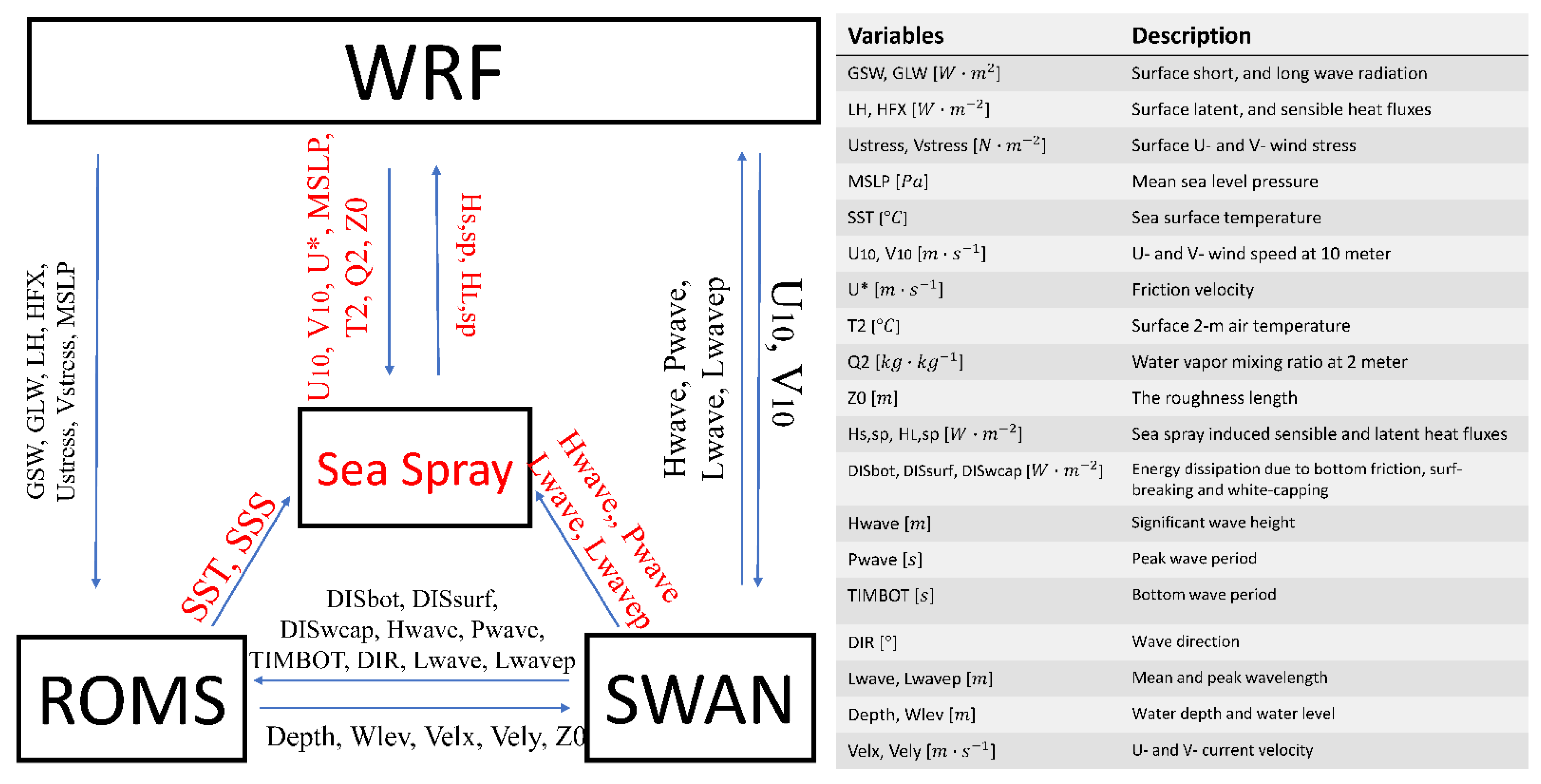
2.1. The Description of Numerical Model

In this study, we adopted the Coupled Ocean-Atmosphere-Wave-Sediment Transport (COAWST) modelling system to investigate the effects of sea spray on an ideal TC system [21] (see the Figure 1). This modelling system comprises three different model components: the atmosphere model (referred to as WRF; the Weather Research Forecasting model), the ocean model (referred to as ROMS; the Regional Ocean Modelling System), and the wave model (referred to as SWAN; the third generation Simulating Wave Nearshore model).

As these three components utilize various prognostic variables to solve the governing equations, we briefly clarify each of them.

1. The atmospheric model used in COAWST is WRF with Advanced Research WRF (ARW) core. WRF is a non-hydrostatic and fully flexible weather forecasting model. Based on the Arakawa-C grid, it generally integrates the Euler equations by using a vertical terrain-following pressure coordinate. WRF includes various modules to parameterize atmospheric physical processes: cumulus, microphysics, surface layer, land-surface layer, planetary boundary layer, and atmospheric radiation. More details about WRF are available in Skamarock et al. [22].

2. The oceanic component used in COAWST is ROMS, which is a three-dimensional numerical model using a generalized vertical, terrain-following, coordinate system. Based on the hydrostatic and Boussinesq assumptions, it solves Reynolds-averaged Navier–Stokes equations [23,24].

3. The SWAN wave numerical model applied in COAWST is a numerical wave model for the realistic estimations of wave properties in the coastal areas [25]. Solving the wave action density balance equation both in spatial and spectral spaces, it includes various sink and source terms, such as the generation of wind waves, wave breaking, and bottom dissipation.

To couple these three components, the Model Coupling Toolkit (MCT) is used as the model coupling tool in COAWST [26,27]. For more information, please refer to [21].

2.2. Sea Spray Models

In COAWST, the COARE bulk algorithm is used to calculate the interfacial air–sea heat flux [28]. However, to characterize the role of sea spray in the air–sea boundary layer, we need to replace the default bulk algorithm with a bulk microphysical algorithm proposed by Andreas, Persson and Hare [5]. To yield predictions of interfacial air–sea heat fluxes, following Perrie [29], we linearly added the net sensible and latent heat flux induced by sea spray to the boundary layer air–sea latent heat flux and sensible heat flux, respectively:

$$H_{L,T}=H_L+H_{L,sp}$$

(8)

$$H_{S,T}=H_S+H_{S,sp}$$

(9)

where $H_{L,T}$ and $H_{S,T}$ are air–sea latent and sensible heat fluxes, respectively; $H_L$ and $H_s$ are the latent and sensible interfacial direct air–sea heat fluxes, respectively. Therefore, based on the sea spray algorithm (i.e., Equations (4)–(7)), and different sea spray volume flux models (i.e., Equations (1) and (2) or Equation (3)), we can estimate the air–sea heat fluxes and include them into the TC forecasting model.

2.3. The Model Configuration and Experimental Design

To initiate an idealized TC system, a bogus asymmetrical vortex at a radius of 50 km with a maximum 10 m wind speed of 20 m s⁻¹ is embedded into a uniform atmospheric environment following Kwok and Chan [30], with a horizontal wind profile set by Chan and Williams [31]. In this environment, uniform moving westerly winds at 5 m s⁻¹ are specified within all atmospheric levels in the simulation domain designed in the WRF (i.e., the atmospheric component of the COAWST). This model domain is centered around ($20°\mathrm{N},37°\mathrm{E}$), covering $2400\times 1800$ km² with $200\times 150$ horizontal grid points (i.e., with a constant resolution of 12 km). A total of 30 vertical levels are utilized in WRF. The water depth is linearly discretized from 1000 to 0 m in the west of this model domain. The WRF Purdue Lin (PL) microphysics scheme [32], Rapid Radiative Transfer Model (RRTM) longwave [33] radiation scheme, Dudhia shortwave [34] radiation scheme, Mellor-Yamada Nakanishi and Niino planetary boundary layer (MYNN) and surface layer schemes [35], and Noah LSM land surface schemes [36] are used in this study. Coupling with WRF, ROMS (i.e., the oceanic component of the COAWST) contains 21 vertical levels with open boundary conditions. For consistency with WRF, ROMS adopts the Cartesian coordinate on an $f$ plane with defining $f=1.45\times {10}^{-4}$. The sea surface temperature (SST) and sea surface salinity (SSS) were defined as 29 °C and 35 PSU, respectively, and they remained constant throughout the integration of modeling. The ocean salinity was uniformly defined, and the water temperature is derived by interpolating from the surface (29 °C) to the bottom (18 °C). In addition, the coordinate system of SWAN (i.e., the wave component of the COAWST), is also defined the same as that in the WRF-ROMS. SWAN utilizes the backward-in-space and backward-in-time advection scheme to integrate circular grids with 36 direction bands. Note that the time steps for integration are 25 s, 25 s, and 300 s for WRF, ROMS, and SWAN, respectively. The forcing fields, between any two of these components, are exchanged every 15 min via the MCT. Please refer to [21,37,38] for more information.

To investigate the effects of the two different sea spray models on a TC system, we conducted three numerical experiments in this study. A 54 h simulation was performed, while, for the analyses, we exclude the initial 12 h which is considered as the spin up time. Expt.1 is defined as the control run without the implementation of the sea spray. In Expt.2, the wave-Reynolds-dependent sea spray model (i.e., Equations (1) and (2)) is considered. Expt.3 considers the wave-steepness-dependent sea spray model (i.e., Equation (3)), see

Table 1. Experimental design in this study.

Experiments	Sea Spray	Sea Spray Model
Expt. 1	No	-
Expt. 2	Yes	Equations (1) and (2)
Expt. 3	Yes	Equation (3)

.

3. Results and Discussion

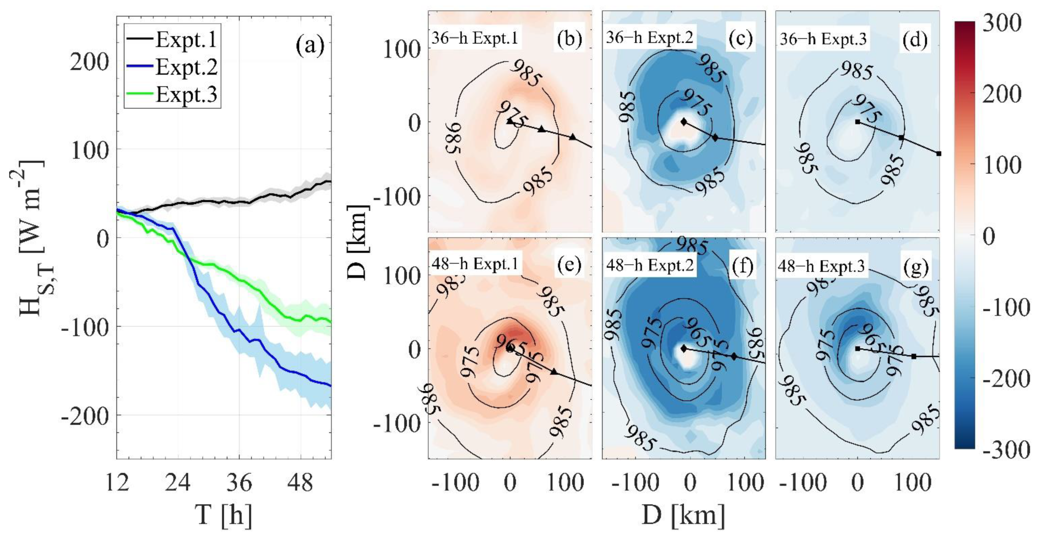
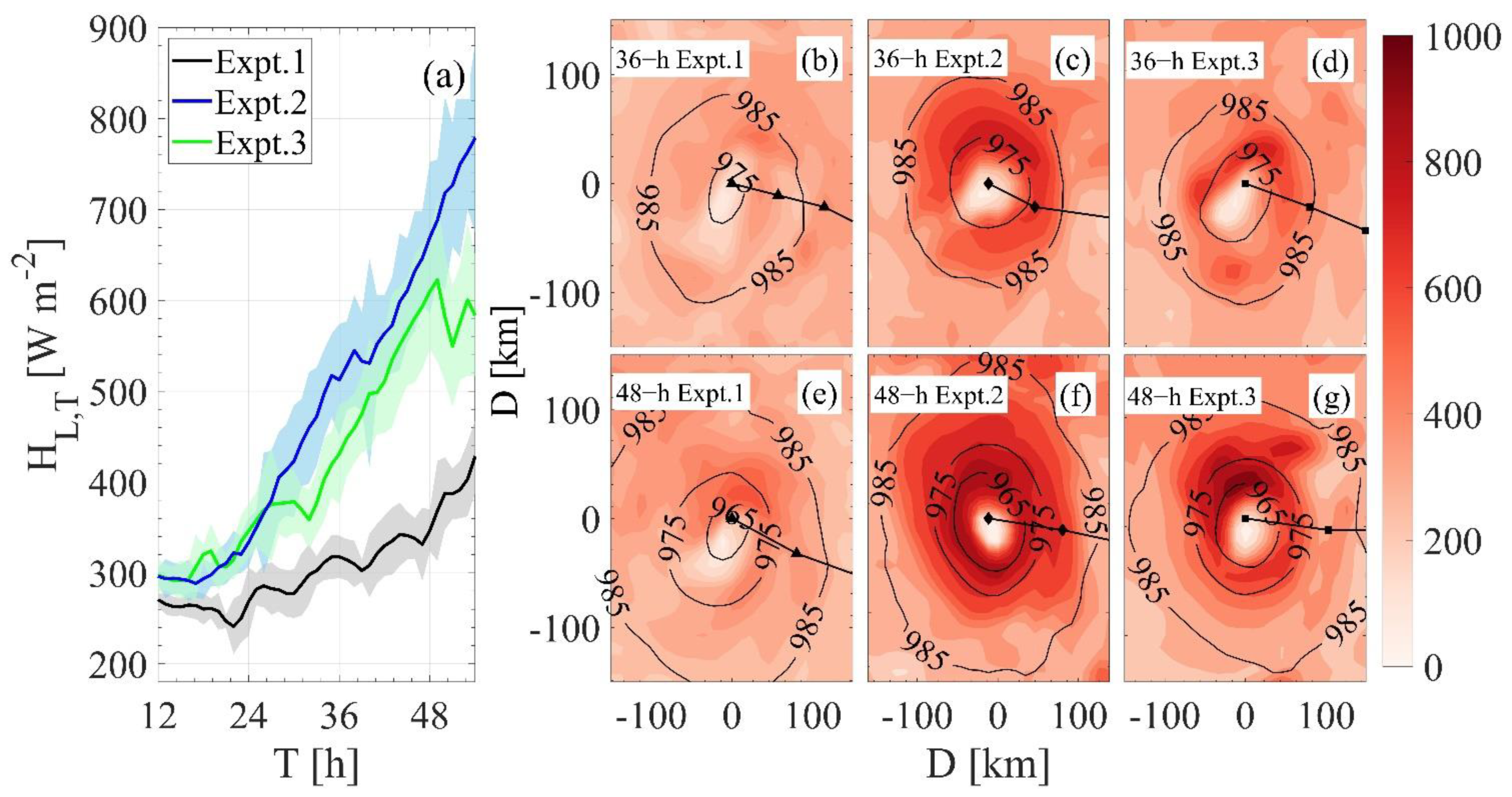
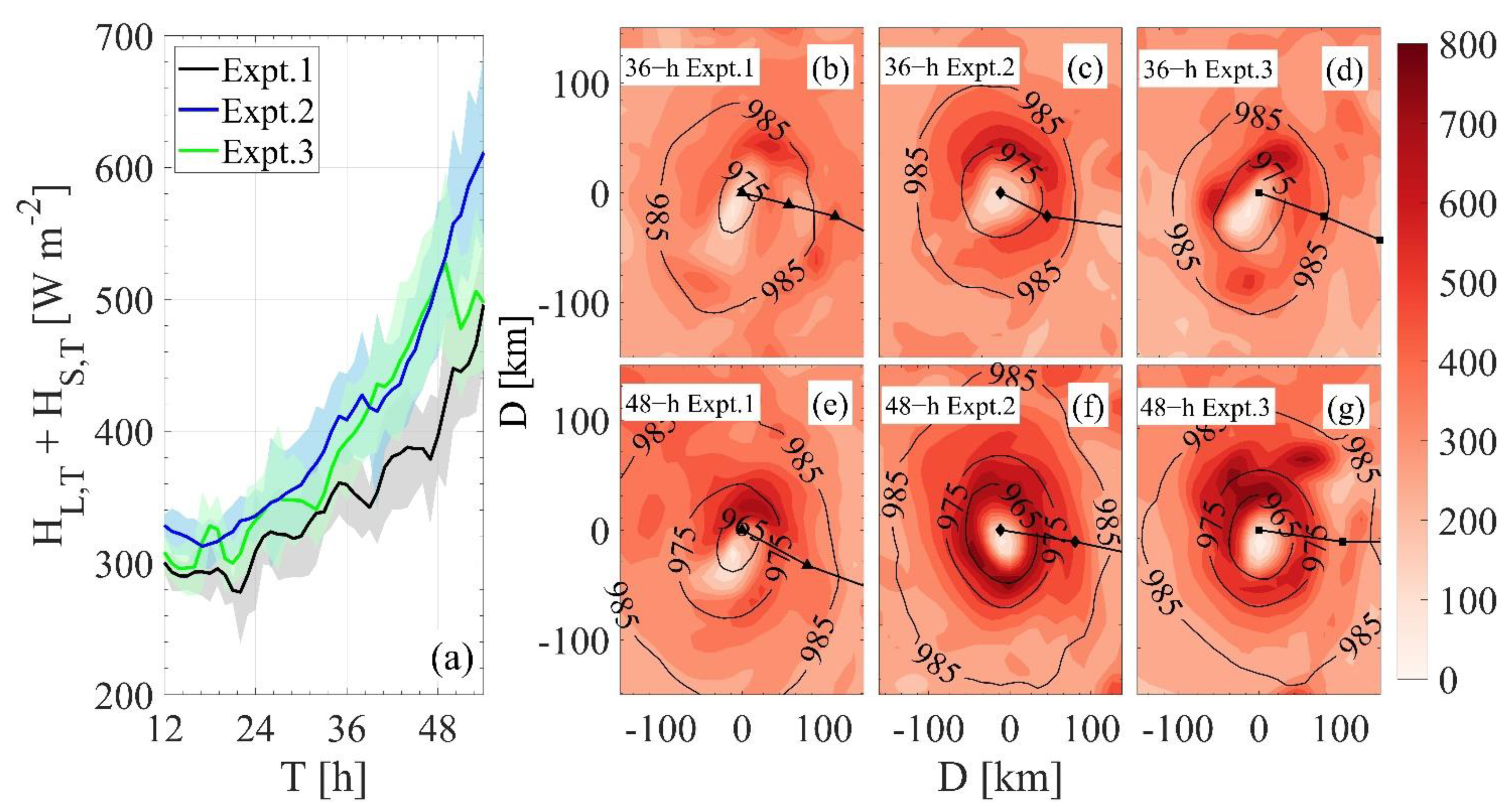
3.1. Impacts on the Air–Sea Heat Flux

Figure 2a shows the integrated air–sea sensible heat flux as a function of the simulation time. Standard deviations are estimated within two times of the radius of maximum wind (RMW) from the center of TCs for the numerical experiments. In comparison to Expt.1, the air–sea sensible heat fluxes decreased by up to 231 W m⁻² (364%) and 159 W m⁻² (251%) in Expt.2 and Expt.3, respectively. This is because the sea spray droplets will partially evaporate once ejected into the air, thereby extracting heat from the atmosphere and lowering the sensible heat in the atmosphere. Spray droplets are expected to transfer sensible heat to the surrounding air as their temperature is higher than the surrounding air, which increases the amount of sensible heat transferred from the ocean to the atmosphere. However, because spray droplet evaporation consumes sensible heat, the air–sea sensible heat fluxes are expected to decrease. Compared with Expt.3, albeit with larger spatial variability (i.e., standard deviation), the sea-spray-induced sensible heat fluxes are larger in Expt.2.

The spatial distribution of sensible heat fluxes after 36 h (b-d) and 48 h (e-g) simulations are depicted in Figure 2b–g. We observe that, under severe atmospheric and oceanic conditions, the sea-spray-induced sensible heat deduction becomes significant within the area surrounding the TC center. Furthermore, in comparison to the results in Expt. 3 (Figure 2d,g), this deduction of air–sea sensible heat fluxes is more significant in Expt. 2 (Figure 2c,f).

Figure 3a shows the integrated air–sea latent heat flux variation with the simulation time. For Expt.2 and Expt.3, the air–sea latent heat fluxes increase by up to 359 W m⁻² (89%) and 263 W m⁻² (76%), respectively. In contrast to its negative contribution of the air-sea sensible heat fluxes, sea spray contributes positively to air–sea latent heat fluxes, and such positive contributions are comparable in magnitude in Expt.2 and Expt.3. However, in comparison to Expt.3, the increase in sea-spray-induced latent heat fluxes occurs over a greater spatial area in Expt.2 (Figure 3c,d,f,g).

As the latent heat flux is considerably larger than the sensible flux, the sea spray increases the total air–sea heat fluxes (Figure 4a). In comparison with Expt.1, while the total air–sea heat fluxes, before around 24 h, are consistent, they are increased, after 24 h, by up to 135 W m⁻² (32%) and 123 W m⁻² (30%) in Expt.2 and Expt.3, respectively. Prior to around 28 h, the total heat fluxes in Expt.2 are comparable to those in Expt.3, but after 28 h, the total heat flux in Expt.2 is greater than in Expt.3, with the exception of the period 38–48 h (Figure 4a).

Figure 4b–g presents the spatial distribution of air–sea total heat fluxes after 36 h (b–d) and 48 h (e–g) simulations, respectively. While sea spray has no discernible effect on the total air–sea heat fluxes after 36 h of simulation (Figure 4b–d), the sea-spray-induced total heat fluxes are noticeable after 48 h of simulation (Figure 4e–g). As illustrated in Figure 4f, in Expt.2, the sea-spray-induced heat fluxes increased in areas centered on the TC eye, whereas in Expt.3 (Figure 4g), the increase is concentrated in the right front quadrant over the TC center, demonstrating the difference in the adoption of various sea spray models.

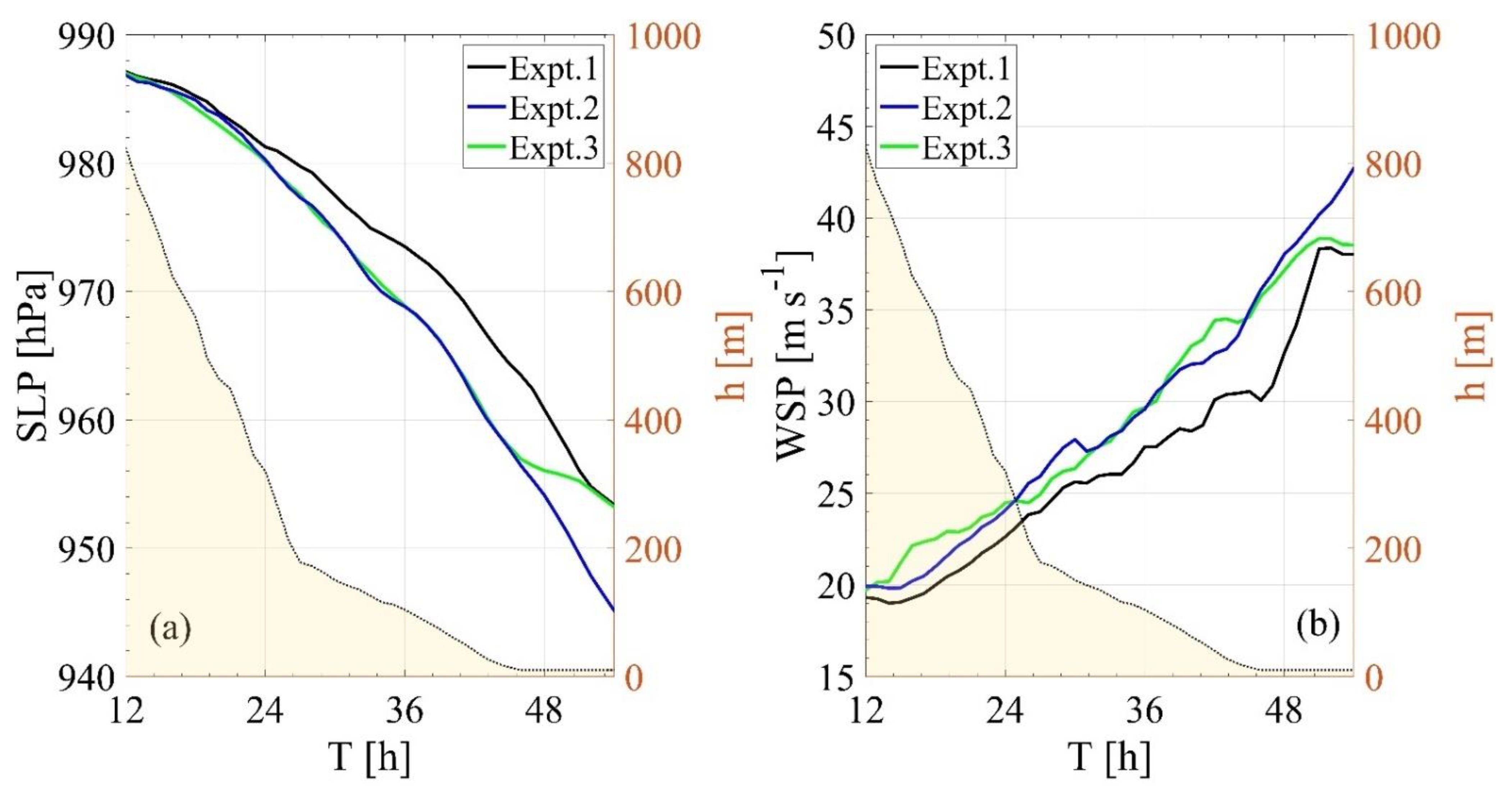
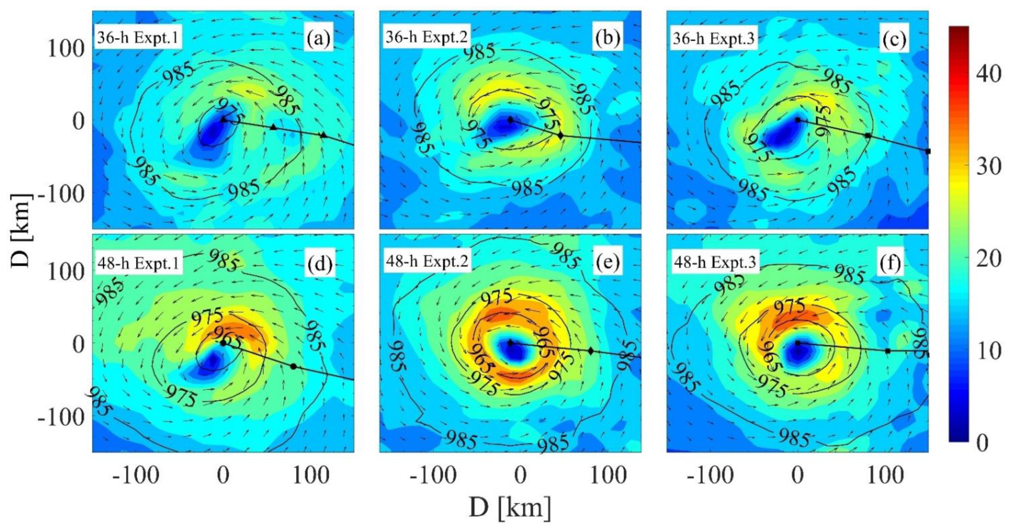
3.2. Impacts on the TC System

As the sea spray increases the total air–sea heat fluxes, it is expected that sea spray has a positive contribution to the development and intensification of the TC system. This can be represented as a decrease in the sea level pressure (SLP). Once the sea spray is included, the minimum SLP is lowered by a maximum of 8 hPa (0.8%) and 7 hPa (0.7%) in Expt.2 and Expt.3, respectively, relative to Expt.1 (Figure 5a). This substantiates the role and importance of sea spray on the development of TC system and is consistent with Andreas, Persson and Hare [5], Perrie [29], Andreas and Emanuel [39], who proposed that incorporating the sea spray increases the maximum TC intensity.

Once the sea spray is considered, the maximum wind speed (WSP) increases by up to 6.4 and 5.8 m s⁻¹ for Expt.2 and Expt.3, respectively (i.e., Figure 5b). Figure 6 shows the spatial distributions of WSP after 36 h and 48 h simulation. Although wind speed increases when sea spray is introduced, the impact of the different sea spray parameterizations leads to spatial differences in the wind field. For example, in Expt.2, the strongest winds are distributed relatively evenly along the quadrants of the TC system (Figure 6e). In contrast, in Expt.3, the wind speed enhancement caused by the sea spray is concentrated in the front quadrant of the TC.

We note that the wind speed is closely related to the momentum transfer from the atmosphere to the ocean. In the present study, effects of sea-spray-induced heat fluxes on the air–sea momentum fluxes are implicit. This is because the heat flux increment caused by sea spray directly influences the TC development, intensification, and local wind field. As such, it has an indirect, rather than direct, influence on the air–sea momentum flux. In addition to indirect dynamic effects, sea spray also directly influences the air–sea momentum, such as by modulating the roughness length [40,41] and increasing/decreasing the net air–sea momentum fluxes [42]. While it is still under debate how the sea spray dynamically affects the air–sea interaction, spray droplets strongly mediate net air–sea momentum fluxes, accounting for up to 16% of the interfacial momentum fluxes [43]. Thus, in addition to thermal effects, direct dynamic effects of sea spray need to be well understood and physically incorporated into the TC modeling.

While sea spray effects strengthen the TC system and increase wind velocity in both Expt.2 and Expt.3, these effects diminish after 50 h simulation in Expt.3. This is attributed to the changes in wave dynamics as the TC system approaches shallow water, thus altering the local wave height and wave steepness. As the sea spray model implemented in Expt.3 is directly related to the wave height, unlike in Expt.2, the sea spray effects in Expt.3 are more pronounced than in Expt.2.

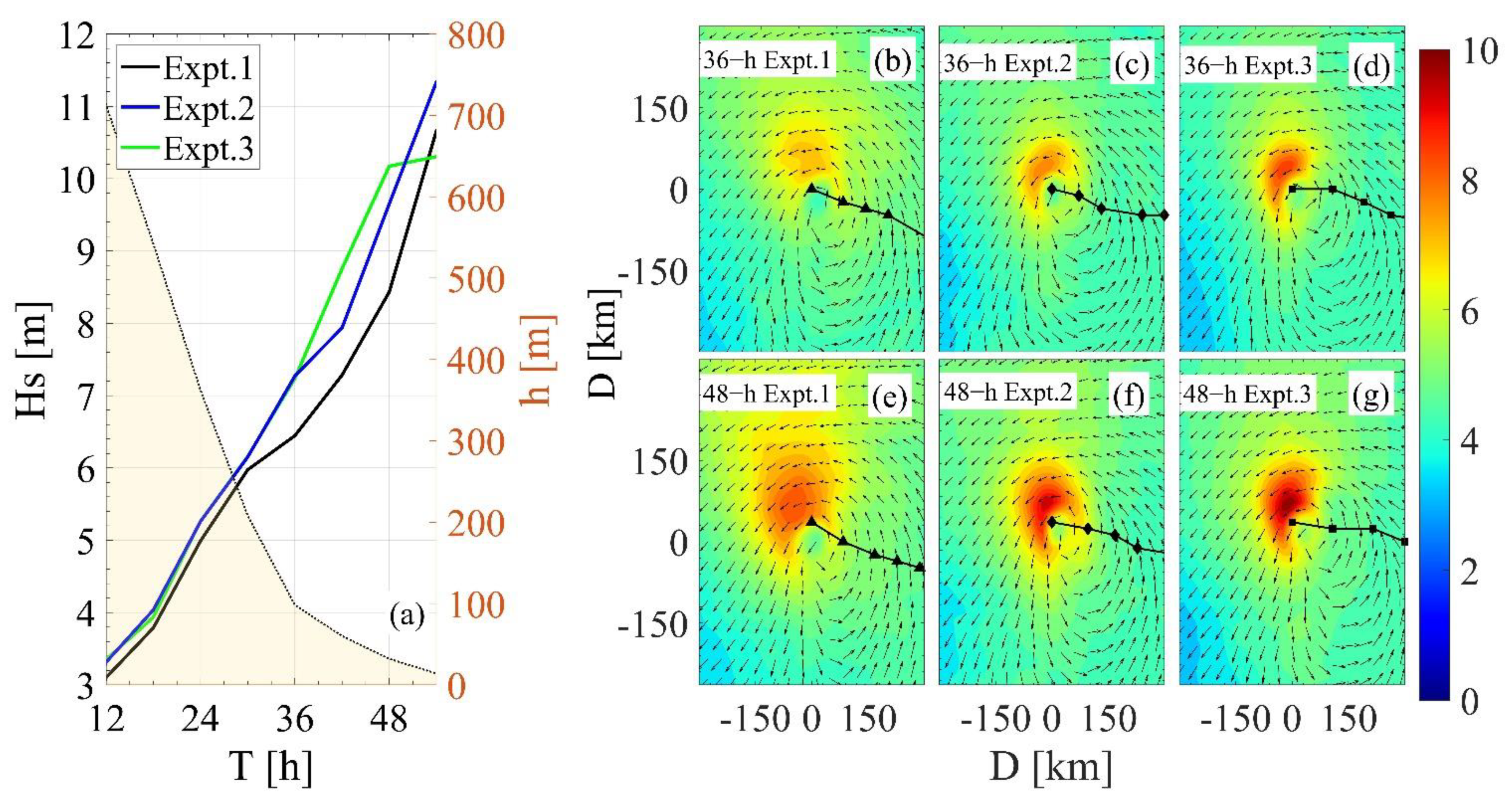
3.3. Impacts on the Ocean Waves

Figure 7a depicts the maximum significant wave height (Hs) with the simulation time. Overall, we observe that the inclusion of the sea spray increases the maximum Hs, specifically, by up to 1.1 m (17%) and 1.6 m (25%) in Expt. 2 and Expt.3, respectively. This is in agreement with Liu, Liu, Xie, Guan and Zhao [18] who observed higher Hs once the sea spray is taken into account when simulating idealized TC cases. Prior to 36 h, the maximum Hs in Expt.2 is consistent with that in Expt.3. For the simulation from 36 h to 52 h, in the comparison with results of Expt.1, impacts of sea spray on Hs are more pronounced in Expt.3 than in Expt.2. After 52 h simulation, while the maximum Hs in Expt.2 remains modestly larger than in Expt.1, the maximum Hs in Expt.3 is smaller than in Expt.1. This demonstrates that the wave-Reynolds-dependent sea spray model positively contributes to the generation of local waves in shallow water through the increase of maximum wind speed. In contrast, the adoption of the wave-steepness-dependent sea spray decreases Hs relative to the reference simulation.

Figure 7b–g shows the spatial distributions of the maximum Hs in Expt.1, Expt.2, and Expt.3 after 36 h, and 48 h simulations, respectively. As we located this idealized TC system in the Northern Hemisphere, maximum Hs is observed in the right front quadrant of the TC track. This is because, in the right front quadrant of the TC track, the wave direction of propagation of locally generated wind sea is consistent with the propagation of (young) swell, which does not occur in other quadrants (as demonstrated in Figure 3 of [44]). In agreement with Figure 7a, sea spray leads indirectly to the enhancement of Hs after both 36 h and 48 h simulations. The increase in maximum Hs is greater in Expt.3 than in Expt.2, highlighting the critical differences in sea spray parameterizations on ocean surface wave fields through sea spray impacts on the wind fields. In comparison to the local wave height, sea spray has a negligible effect on the direction of the waves (see Figure 7b–g).

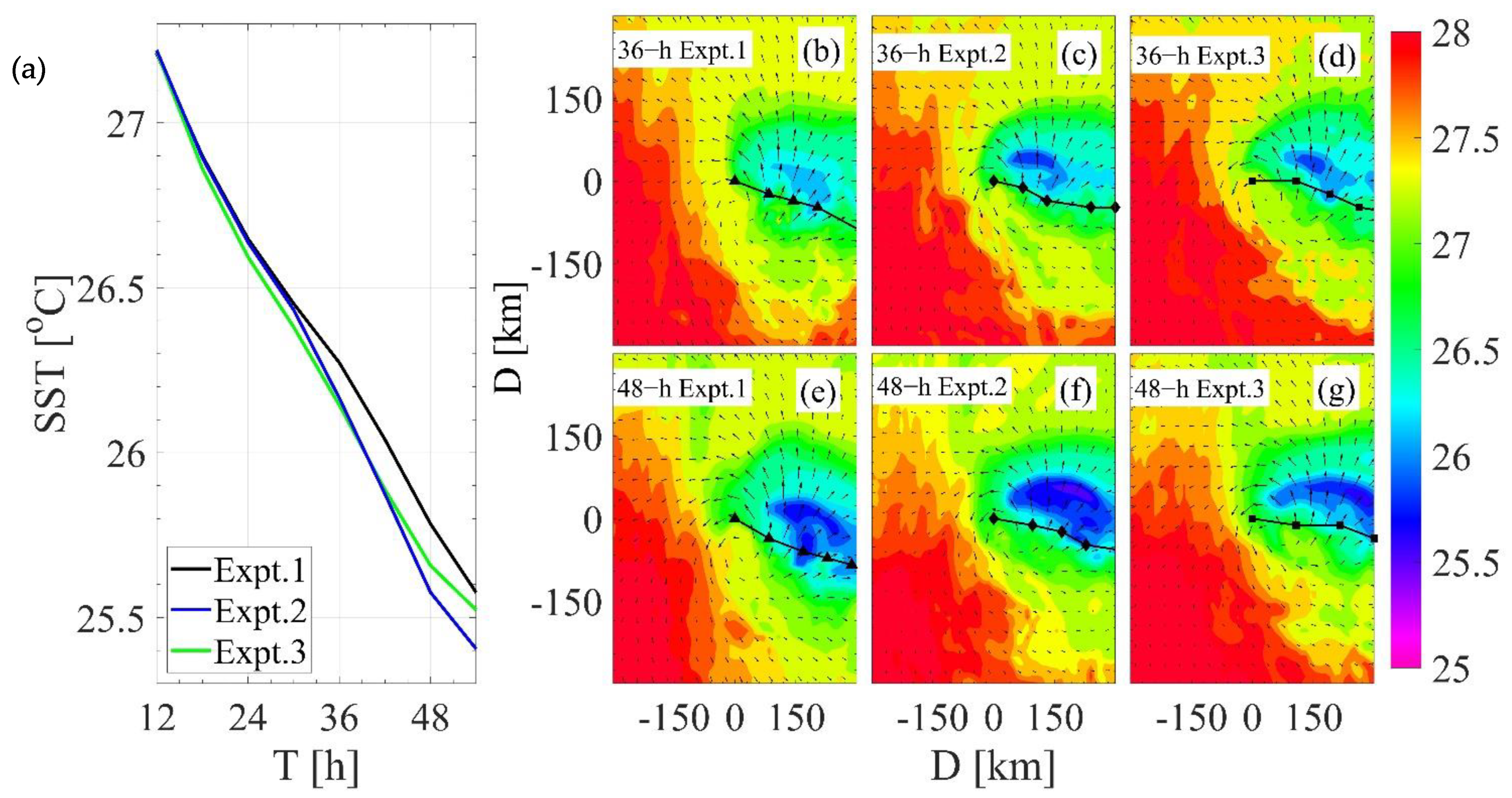
3.4. Impacts on the SST

Figure 8a shows the minimum SST variation with the model simulation time for Expt.1, Expt.2, and Expt.3. The SST is expected to decrease during the passage of the TC system as deep cold water rises to the ocean surface as a result of turbulent mixing and upwelling. Compared with the minimum SST in Expt.1, the minimum SST is reduced by up to 0.2 °C (0.8%) and 0.15 °C (0.6%) in Expt.2 and Expt.3, respectively. This is a direct result of the sea-spray-induced intensification of the TC system, which in turn positively contributes to the vertical turbulent mixing over the upper ocean. Note, this is in line with other studies which suggest that sea spray strengthens the SST cooling during TC passing [18,29,43]. To further explore the impacts of sea spray on the SST, the spatial distributions of SST during the TC passing are shown in Figure 8b–g. We notice that areas where the SST is reduced are located on the right side of the TC track. This rightward difference is caused by the acceleration of inertial currents due to the rotation of the wind stress vector. Including sea spray physics decreases the minimum SST during the TC passing and expands the surface area of minimum SST in the wake of the TC system. Additionally, we observe that sea-spray-induced SST reduction is more pronounced in Expt.2 than in Expt.3 (Figure 8f–g), indicating that the influence of the wave-Reynolds-dependent sea spray parameterization on the SST is more pronounced. This is because of stronger turbulent mixing and upwelling in Expt.2 in comparison with Expt.3. As shown in Figure 6e–f, the wind speed increase caused by sea spray is more noticeable in Expt.2 compared to Expt.3. This contributes to a larger momentum transfer from the atmosphere to the ocean in Expt.2 in contrast to Expt.3. As the air–sea momentum fluxes contribute significantly to the stirring of warm surface water with cooler water in the thermocline, SST reduction should be more pronounced in Expt.2 than in Expt.3.

4. Summary and Conclusions

This study uses a coupled air–sea–wave numerical model to investigate the impact of sea spray on the air–sea environments of an idealized TC case. To do so, two sea spray parameterizations are implemented: a wave-Reynolds-dependent and a wave-steepness-dependent sea spray model (Expt. 2 and 3, respectively). Based on these sea spray models, we analyzed the atmospheric and oceanic properties during an idealized TC case to the thermal effects induced by the sea spray.

Results show that the introduction of sea spray decreases the air–sea sensible heat fluxes by up to 231 W m⁻² (364%) and 159 W m⁻² (251%) for Expt.2 and Expt.3, respectively. At the same time, the latent heat fluxes at the air–sea surface are increased by up to 359 W m⁻² (89%) and 263 W m⁻² (76%), for Expt.2 and Expt.3, respectively. As a result, the total air–sea heat fluxes are increased by up to 135 W m⁻² (32%) and 123 W m⁻² (30%) for Expt.2 and Expt.3, respectively.

By considering the thermal effects of the sea spray, the minimum SLP is reduced by up to 8 hPa (0.8%) and 7 hPa (0.7%) and maximum wind speed is increased by up to 6.1 m s⁻¹ (20%) and 5.7 m s⁻¹ (19%), in Expt.2 and Expt.3, respectively. This suggests that sea spray positively contributes to the development of the TC system through increased air–sea heat fluxes. The increases in wind speed ultimately lead to larger waves, with Hs rising by up to 1.1 m (17%) and 1.6 m (25%), for Expt.2 and Expt.3, respectively. As the production of sea spray largely depends on the local wind and wave conditions, it is expected that the sea-spray-induced WSP increasing and Hs rising lead to further positive feedback on the generation of sea spray.

In addition to local winds and waves, sea spray indirectly influences the SST. When the sea spray is considered, the ocean surface cooling during the passage of TC system is enhanced (i.e., the minimum SST decreasing by a maximum of 0.2 °C (0.8%) and 0.15 °C (0.6%) for Expt.2 and Expt.3, respectively). Therefore, as sea spray dramatically affects the atmospheric and oceanic environments by modulating the wind speed, Hs, and SST, it needs to be incorporated into operational TC forecasting models and future studies are required to assess the impact of wave-dependent sea spray parameterizations on real TCs.

References

1. Veron, F. Ocean Spray. Annu. Rev. Fluid Mech. 2015, 47, 507–538. [Google Scholar] [CrossRef]
2. Mueller, J.A.; Veron, F. Impact of sea spray on air–sea fluxes. Part II: Feedback effects. J. Phys. Oceanogr. 2014, 44, 2835–2853. [Google Scholar] [CrossRef]
3. Veron, F.; Hopkins, C.; Harrison, E.L.; Mueller, J.A. Sea spray spume droplet production in high wind speeds. Geophys. Res. Lett. 2012, 39. [Google Scholar] [CrossRef] [Green Version]
4. Troitskaya, Y.; Druzhinin, O.; Kozlov, D.; Zilitinkevich, S. The “Bag Breakup” Spume Droplet Generation Mechanism at High Winds. Part II: Contribution to Momentum and Enthalpy Transfer. J. Phys. Oceanogr. 2018, 48, 2189–2207. [Google Scholar] [CrossRef]
5. Andreas, E.L.; Persson, P.O.G.; Hare, J.E. A Bulk Turbulent Air–Sea Flux Algorithm for High-Wind, Spray Conditions. J. Phys. Oceanogr. 2008, 38, 1581–1596. [Google Scholar] [CrossRef]
6. Zhang, L.; Zhang, X.; Chu, P.C.; Guan, C.; Fu, H.; Chao, G.; Han, G.; Li, W. Impact of sea spray on the Yellow and East China Seas thermal structure during the passage of Typhoon Rammasun. J. Geophys. Res. Ocean. 2017, 122, 7783–7802. [Google Scholar] [CrossRef] [Green Version]
7. Bao, J.W.; Fairall, C.W.; Michelson, S.A.; Bianco, L. Parameterizations of Sea-Spray Impact on the Air–Sea Momentum and Heat Fluxes. Mon. Weather Rev. 2011, 139, 3781–3797. [Google Scholar] [CrossRef]
8. Bao, J.; Wilczak, J.; Choi, J.; Kantha, L. Numerical simulations of air–sea interaction under high wind conditions using a coupled model: A study of hurricane development. Mon. Weather Rev. 2000, 128, 2190–2210. [Google Scholar] [CrossRef]
9. Wu, L.C.; Rutgersson, A.; Sahlee, E.; Larsen, X.G. The impact of waves and sea spray on modelling storm track and development. Tellus Ser. A-Dyn. Meteorol. Oceanogr. 2015, 67. [Google Scholar] [CrossRef] [Green Version]
10. Rizza, U.; Canepa, E.; Miglietta, M.M.; Passerini, G.; Morichetti, M.; Mancinelli, E.; Virgili, S.; Besio, G.; De Leo, F.; Mazzino, A. Evaluation of drag coefficients under medicane conditions: Coupling waves, sea spray and surface friction. Atmos. Res. 2021, 247, 105207. [Google Scholar] [CrossRef]
11. Rizza, U.; Canepa, E.; Ricchi, A.; Bonaldo, D.; Carniel, S.; Morichetti, M.; Passerini, G.; Santiloni, L.; Scremin Puhales, F.; Miglietta, M.M. Influence of wave state and sea spray on the roughness length: Feedback on medicanes. Atmosphere 2018, 9, 301. [Google Scholar] [CrossRef] [Green Version]
12. Perrie, W.; Zhang, W.; Andreas, E.L.; Li, W.; Gyakum, J.; McTaggart-Cowan, R. Sea spray impacts on intensifying midlatitude cyclones. J. Atmos. Sci. 2005, 62, 1867–1883. [Google Scholar] [CrossRef]
13. Monahan, E.C.; Davidson, K.L.; Spiel, D.E. Whitecap aerosol productivity deduced from simulation tank measurements. J. Geophys. Res. Ocean. 1982, 87, 8898–8904. [Google Scholar] [CrossRef]
14. Norris, S.J.; Brooks, I.M.; Salisbury, D.J. A wave roughness Reynolds number parameterization of the sea spray source flux. Geophys. Res. Lett. 2013, 40, 4415–4419. [Google Scholar] [CrossRef] [Green Version]
15. Lenain, L.; Melville, W.K. Evidence of Sea-State Dependence of Aerosol Concentration in the Marine Atmospheric Boundary Layer. J. Phys. Oceanogr. 2017, 47, 69–84. [Google Scholar] [CrossRef]
16. Zhao, D.; Toba, Y. Dependence of whitecap coverage on wind and wind-wave properties. J. Oceanogr. 2001, 57, 603–616. [Google Scholar] [CrossRef]
17. Zhao, D.; Toba, Y.; Sugioka, K.-i.; Komori, S. New sea spray generation function for spume droplets. J. Geophys. Res. 2006, 111. [Google Scholar] [CrossRef]
18. Liu, B.; Liu, H.; Xie, L.; Guan, C.; Zhao, D. A Coupled Atmosphere–Wave–Ocean Modeling System: Simulation of the Intensity of an Idealized Tropical Cyclone. Mon. Weather Rev. 2011, 139, 132–152. [Google Scholar] [CrossRef]
19. Xu, X.; Voermans, J.J.; Ma, H.; Guan, C.; Babanin, A.V. A Wind–Wave-Dependent Sea Spray Volume Flux Model Based on Field Experiments. J. Mar. Sci. Eng. 2021, 9, 1168. [Google Scholar] [CrossRef]
20. Andreas, E.L. Sea Spray and the Turbulent Air-Sea Heat Fluxes. J. Geophys. Res. 1992, 97, 11429–11441. [Google Scholar] [CrossRef]
21. Warner, J.C.; Armstrong, B.; He, R.; Zambon, J.B. Development of a Coupled Ocean–Atmosphere–Wave–Sediment Transport (COAWST) Modeling System. Ocean Model. 2010, 35, 230–244. [Google Scholar] [CrossRef] [Green Version]
22. Skamarock, W.; Klemp, J.; Dudhia, J.; Gill, D.; Barker, D.; Wang, W.; Powers, J. A Description of the Advanced Research WRF Version 3; NCAR Technical Note NCAR/TN-4751STR; National Center for Atmospheric Research: Boulder, CO, USA, 2008. [Google Scholar]
23. Chassignet, E.P.; Arango, H.; Dietrich, D.; Ezer, T.; Ghil, M.; Haidvogel, D.B.; Ma, C.-C.; Mehra, A.; Paiva, A.M.; Sirkes, Z. DAMEE-NAB: The base experiments. Dyn. Atmos. Ocean. 2000, 32, 155–183. [Google Scholar] [CrossRef]
24. Haidvogel, D.B.; Arango, H.G.; Hedstrom, K.; Beckmann, A.; Malanotte-Rizzoli, P.; Shchepetkin, A.F. Model evaluation experiments in the North Atlantic Basin: Simulations in nonlinear terrain-following coordinates. Dyn. Atmos. Ocean. 2000, 32, 239–281. [Google Scholar] [CrossRef]
25. Booij, N.; Holthuijsen, L.; Ris, R. The “SWAN” wave model for shallow water. In Proceedings of the 25th International Conference on Coastal Engineering, Orlando, FL, USA, 2–6 September 1996; pp. 668–676. [Google Scholar]
26. Larson, J.; Jacob, R.; Ong, E. The model coupling toolkit: A new Fortran90 toolkit for building multiphysics parallel coupled models. Int. J. High Perform. Comput. Appl. 2005, 19, 277–292. [Google Scholar] [CrossRef]
27. Jacob, R.; Larson, J.; Ong, E. M × N communication and parallel interpolation in Community Climate System Model Version 3 using the model coupling toolkit. Int. J. High Perform. Comput. Appl. 2005, 19, 293–307. [Google Scholar] [CrossRef]
28. Fairall, C.W.; Bradley, E.F.; Rogers, D.P.; Edson, J.B.; Young, G.S. Bulk parameterization of air-sea fluxes for Tropical Ocean-Global Atmosphere Coupled-Ocean Atmosphere Response Experiment. J. Geophys. Res. Ocean. 1996, 101, 3747–3764. [Google Scholar] [CrossRef]
29. Perrie, W. Simulation of extratropical Hurricane Gustav using a coupled atmosphere-ocean-sea spray model. Geophys. Res. Lett. 2004, 31. [Google Scholar] [CrossRef]
30. Kwok, J.H.; Chan, J.C. The influence of uniform flow on tropical cyclone intensity change. J. Atmos. Sci. 2005, 62, 3193–3212. [Google Scholar] [CrossRef]
31. Chan, J.C.; Williams, R. Analytical and numerical studies of the beta-effect in tropical cyclone motion. Part I: Zero mean flow. J. Atmos. Sci. 1987, 44, 1257–1265. [Google Scholar] [CrossRef] [Green Version]
32. Lin, Y.-L.; Farley, R.D.; Orville, H.D. Bulk Parameterization of the Snow Field in a Cloud Model. J. Appl. Meteorol. Climatol. 1983, 22, 1065–1092. [Google Scholar] [CrossRef] [Green Version]
33. Mlawer, E.J.; Taubman, S.J.; Brown, P.D.; Iacono, M.J.; Clough, S.A. Radiative transfer for inhomogeneous atmospheres: RRTM, a validated correlated-k model for the longwave. J. Geophys. Res. Atmos. 1997, 102, 16663–16682. [Google Scholar] [CrossRef] [Green Version]
34. Dudhia, J. Numerical study of convection observed during the winter monsoon experiment using a mesoscale two-dimensional model. J. Atmos. Sci. 1989, 46, 3077–3107. [Google Scholar] [CrossRef]
35. Nakanishi, M.; Niino, H. An improved Mellor–Yamada level-3 model: Its numerical stability and application to a regional prediction of advection fog. Bound.-Layer Meteorol. 2006, 119, 397–407. [Google Scholar] [CrossRef]
36. Chen, F.; Dudhia, J. Coupling an advanced land surface–hydrology model with the Penn State–NCAR MM5 modeling system. Part I: Model implementation and sensitivity. Mon. Weather Rev. 2001, 129, 569–585. [Google Scholar] [CrossRef] [Green Version]
37. Warner, J.C.; Sherwood, C.R.; Signell, R.P.; Harris, C.K.; Arango, H.G. Development of a three-dimensional, regional, coupled wave, current, and sediment-transport model. Comput. Geosci. 2008, 34, 1284–1306. [Google Scholar] [CrossRef]
38. Zambon, J.B.; He, R.; Warner, J.C. Investigation of hurricane Ivan using the coupled ocean–atmosphere–wave–sediment transport (COAWST) model. Ocean Dyn. 2014, 64, 1535–1554. [Google Scholar] [CrossRef]
39. Andreas, E.L.; Emanuel, K.A. Effects of Sea Spray on Tropical Cyclone Intensity. J. Atmos. Sci. 2001, 58, 3741–3751. [Google Scholar] [CrossRef] [Green Version]
40. Liu, B.; Ding, Y.; Guan, C. A relationship between wave steepness and wave age for wind waves in deep water. Chin. J. Oceanol. Limnol. 2007, 25, 36–41. [Google Scholar] [CrossRef]
41. Powell, M.D.; Vickery, P.J.; Reinhold, T.A. Reduced drag coefficient for high wind speeds in tropical cyclones. Nature 2003, 422, 279–283. [Google Scholar] [CrossRef]
42. Sroka, S.; Emanuel, K. A Review of Parameterizations for Enthalpy and Momentum Fluxes from Sea Spray in Tropical Cyclones. J. Phys. Oceanogr. 2021, 51, 3053–3069. [Google Scholar] [CrossRef]
43. Zhang, L.; Zhang, X.; Perrie, W.; Guan, C.; Dan, B.; Sun, C.; Wu, X.; Liu, K.; Li, D. Impact of Sea Spray and Sea Surface Roughness on the Upper Ocean Response to Super Typhoon Haitang. J. Phys. Oceanogr. 2021, 51, 1929–1945. [Google Scholar] [CrossRef]
44. Holthuijsen, L.H.; Powell, M.D.; Pietrzak, J.D. Wind and waves in extreme hurricanes. J. Geophys. Res. Ocean. 2012, 117. [Google Scholar] [CrossRef] [Green Version]
Figure 1. Schematic illustration of the numerical model used in this study (modified after Warner, Armstrong, He and Zambon [21]. H L , s p and H S , s p are the net latent and sensible heat fluxes induced by the sea spray, respectively (see Equations (6) and (7)). For other coupling parameters exchanged between each of the components, please refer to Warner, Armstrong, He and Zambon [21].
Jmse 09 01390 g001
Figure 2. (a) The integrated air–sea sensible heat fluxes with the simulation time for the Expt.1, Expt.2, and Expt.3. Solid lines and shadows mark the mean and standard deviation of the area-averages within two times of the radius of maximum wind (RMW) from the center of TCs for the numerical experiments. (bd) The spatial distributions of air–sea sensible heat fluxes (shadowing at the interval of 10 W m−2) and sea level pressure (SLP) (contouring at the interval of 10 hPa) with the 6 h TC tracks (black line with the triangle, diamond, and square markers) after 36 h simulation for Expt.1, Expt.2, and Expt.3, respectively. (eg) The spatial distributions of air–sea sensible heat fluxes (shadowing at the interval of 10 W m−2) and sea level pressure (SLP) (contouring at the interval of 10 hPa) with the 6 h TC tracks (black line with the triangle, diamond, and square markers) after 48 h simulation for Expt.1, Expt.2, and Expt.3, respectively. Note, the tracks of TC are from the right to the left following the black line.
Jmse 09 01390 g002
Figure 3. (a) The integrated air–sea latent heat fluxes with the simulation time for the Expt.1, Expt.2, and Expt.3. Solid lines and shadows mark the mean and standard deviation of the area-averages within two times of the radius of maximum wind (RMW) from the center of TCs for the numerical experiments. (bd) The spatial distributions of air–sea latent heat fluxes (shadowing at the interval of 10 W m−2) and sea level pressure (SLP) (contouring at the interval of 10 hPa) with the 6 h TC tracks (black line with the triangle, diamond, and square markers) after 36 h simulation for Expt.1, Expt.2, and Expt.3, respectively. (eg) The spatial distributions of air–sea latent heat fluxes (shadowing at the interval of 10 W m−2) and sea level pressure (SLP) (contouring at the interval of 10 hPa) with the 6 h TC tracks (black line with the triangle, diamond, and square markers) after 48 h simulation for Expt.1, Expt.2, and Expt.3, respectively. Note, the tracks of TC are from the right to the left following the black line.
Jmse 09 01390 g003
Figure 4. (a) The integrated air–sea total heat fluxes with the simulation time for the Expt.1, Expt.2, and Expt.3. Solid lines and shadows mark the mean and standard deviation of the area-averages within two times of the radius of maximum wind (RMW) from the center of TCs for the numerical experiments. (bd) The spatial distributions of air–sea total heat fluxes (shadowing at the interval of 10 W m−2) and sea level pressure (SLP) (contouring at the interval of 10 hPa) with the 6 h TC tracks (black line with the triangle, diamond, and square markers) after 36 h simulation for Expt.1, Expt.2, and Expt.3, respectively. (eg) The spatial distributions of air–sea total heat fluxes (shadowing at the interval of 10 W m−2) and sea level pressure (SLP) (contouring at the interval of 10 hPa) with the 6 h TC tracks (black line with the triangle, diamond, and square markers) after 48 h simulation for Expt.1, Expt.2, and Expt.3, respectively. Note, the tracks of TC are from the right to the left following the black line.
Jmse 09 01390 g004
Figure 5. (a) The minimum sea level pressure (SLP) varies with the simulation time for the Expt.1, Expt.2, and Expt.3, respectively. (b) same as (a), but for the maximum 10 m wind speed (WSP). In each plot, the border of the shadow area indicates the local water depth around the TC center of Expt.1.
Jmse 09 01390 g005
Figure 6. (ac) The spatial distributions of wind speed (WSP) (shadowing at the interval of 10 m s−1), local wind direction (vector), and SLP (contouring at the interval of 10 hPa) with the 6 h TC tracks (black line with the triangle, diamond, and square sign) after 36 h simulation for Expt.1, Expt.2, and Expt.3, respectively. (df) same as (ac), but for the simulation after 48 h simulations.
Jmse 09 01390 g006
Figure 7. (a) The maximum significant wave height (Hs) with the simulation time for the Expt.1, Expt.2, and Expt.3. The border of the shadow area indicates the local water depth around the TC center of Expt.1. (bd) The spatial distributions of Hs with the 6 h TC tracks (black line with the triangle, diamond, and square markers) after 36h simulation for Expt.1, Expt.2, and Expt.3, respectively. (eg) The spatial distributions of Hs with the 6 h TC tracks (black line with the triangle, diamond, and square markers) after 48h simulation for Expt.1, Expt.2, and Expt.3, respectively. Note, the tracks of TC are from the right to the left following the black line.
Jmse 09 01390 g007
Figure 8. (a) The minimum sea surface temperature (SST) with the simulation time for the Expt.1, Expt.2, and Expt.3. (bd) The spatial distributions of SST with the 6 h TC tracks (black line with the triangle, diamond, and square markers) after 36h simulation for Expt.1, Expt.2, and Expt.3, respectively. (eg) The spatial distributions of SST with the 6 h TC tracks (black line with the triangle, diamond, and square markers) after 48h simulation for Expt.1, Expt.2, and Expt.3, respectively. Note, the tracks of TC are from the right to the left following the black line.
Jmse 09 01390 g008