Categorizing Active Marine Acoustic Sources Based on Their Potential to Affect Marine Animals

Abstract

Marine acoustic sources are widely used for geophysical imaging, oceanographic sensing, and communicating with and tracking objects or robotic vehicles in the water column. Under the U.S. Marine Mammal Protection Act and similar regulations in several other countries, the impact of controlled acoustic sources is assessed based on whether the sound levels received by marine mammals meet the criteria for harassment that causes certain behavioral responses. This study describes quantitative factors beyond received sound levels that could be used to assess how marine species are affected by many commonly deployed marine acoustic sources, including airguns, high-resolution geophysical sources (e.g., multibeam echosounders, sidescan sonars, subbottom profilers, boomers, and sparkers), oceanographic instrumentation (e.g., acoustic doppler current profilers, split-beam fisheries sonars), and communication/tracking sources (e.g., acoustic releases and locators, navigational transponders). Using physical criteria about the sources, such as source level, transmission frequency, directionality, beamwidth, and pulse repetition rate, we divide marine acoustic sources into four tiers that could inform regulatory evaluation. Tier 1 refers to high-energy airgun surveys with a total volume larger than 1500 in³ (24.5 L) or arrays with more than 12 airguns, while Tier 2 covers the remaining low/intermediate energy airgun surveys. Tier 4 includes most high-resolution geophysical, oceanographic, and communication/tracking sources, which are considered unlikely to result in incidental take of marine mammals and therefore termed de minimis. Tier 3 covers most non-airgun seismic sources, which either have characteristics that do not meet the de minimis category (e.g., some sparkers) or could not be fully evaluated here (e.g., bubble guns, some boomers). We also consider the simultaneous use of multiple acoustic sources, discuss marine mammal field observations that are consistent with the de minimis designation for some acoustic sources, and suggest how to evaluate acoustic sources that are not explicitly considered here.

1. Introduction

A wide range of controlled sound sources is deployed in the marine environment to map, explore, and characterize the seafloor, the subbottom, and the water column and to communicate with or track remote devices (e.g., remotely operated vehicles, seafloor sensors) that are also used to accomplish these tasks. For controlled sound sources, physical factors such as the power level, transmission frequency, duration of sound pulses, and deployment depth, as well as characteristics of the seafloor and seawater, influence sound propagation in the marine environment. An animal’s response to a sound source depends on the biological characteristics (e.g., hearing range and sensitivity, behavioral activity) and the environmental context (e.g., depth in the water column, distance from the source) of the marine species receiving the sound. The combination of the physics of the sound sources and the biological aspects of the receivers determines how sound sources may affect marine species, some of which are protected by United States (USA) environmental laws such as the Marine Mammal Protection Act (MMPA) and the Endangered Species Act (ESA).

This paper focuses on the impact of active acoustic sources on animals in the marine environment, with an emphasis on the measurable, quantifiable, physical characteristics of sound sources, rather than on the biological characteristics of species and their behavioral responses (e.g., [1]). Due to significant knowledge gaps in biology and animal behavior, researchers, private companies, and federal and state agencies that deploy similar marine acoustic sources sometimes reach different conclusions about their potential level of impact. Rigorous analysis of the physical characteristics of the sound sources and their likely impact could reduce some of the uncertainty associated with the application of regulatory thresholds for harassment of marine species. To develop a more uniform framework for assessing the impact of acoustic sources on marine species, we devise factors that can be used to assign these sources to tiers, ranging from highest (Tier 1) impact to lowest or de minimis effects (Tier 4; unlikely to result in incidental take of marine mammals according to U.S. legislation).

This paper is focused on acoustic sources commonly used in marine geophysics and oceanography. More broadly, anthropogenic sound in the marine environment can be either an unintended byproduct of activities or deliberately controlled. For example, byproduct sounds from shipping, seafloor drilling, or installation of infrastructure are not integral to the purpose of the activity. The sources we focus on in this paper introduce sound into the water column to achieve a specific measurement, monitoring need, or instrument communication/tracking goal. Such acoustic sources are widely used to image the physical environment below the seafloor, at the seafloor itself, or in the water column, or to non-destructively measure physical parameters (e.g., subbottom properties, sound speed in water, current velocity, seafloor or water column backscatter). Controlled sources are also deployed to locate, retrieve, or navigate marine equipment in the water column or at the seafloor and to interrogate monitoring equipment that can send data to the ocean’s surface telemetrically.

This paper first introduces background information on the characterization of anthropogenic marine sounds, the current environmental statutes applied by the U.S. government, and the broad classes of acoustic sources that we analyze. We then evaluate sound sources based on quantitative criteria, comparing the effects to thresholds currently used to implement the MMPA, and conclude that many widely used, non-airgun sources are unlikely to result in incidental take of marine mammals. Following this analysis, we describe proposed tiers for marine acoustic sources and potential approaches for evaluation of each tier based on their predicted level of impact. We also address the simultaneous use of multiple acoustic sources and discuss observational data that support our findings that some classes of acoustic sources are unlikely to result in the incidental take of marine mammals.

2. Background

2.1. Characterizing Marine Sound

This section defines the acoustic terminology used in this paper, which closely follows marine acoustics conventions rather than the way in which metrics are applied in the U.S. marine regulatory community. Acoustic sources are often characterized according to the magnitude of the acoustic intensity (W/m²) they generate at a receiver (e.g., a marine animal). By convention, this characterization uses decibels, a unit that depends on the ratio of sound intensities (or levels) and that is typically defined as $10{\log }_{10}\left(I/I_{ref}\right)$ [2,3,4,5], where $I$ is the intensity of the acoustic wave and $I_{ref}$ denotes a reference intensity. The nominal definition for sound pressure level (SPL) is:

$$SPL=10{\log }_{10}\left(\frac{I}{I_{ref}}\right)=20{\log }_{10}\left(\frac{P_e}{P_{ref}}\right),$$

(1)

where P_e is a root-mean-squared (rms) pressure and P_ref represents reference pressure. The SPL in (1) is also sometimes called the SPL_rms in the U.S. regulatory community. Equation (1) applies to plane and spherical waves (the only types considered here), and $I_{ref}$ in (1) refers to a plane wave whose rms pressure or reference pressure P_ref is equal to 1 μPa [2,3,4,5]. This definition is suitable for many acoustic sources (e.g., multibeam echosounders), particularly those that are narrowband (e.g., the bandwidth is a small fraction of the center frequency). However, the definition may be inadequate for assessing the potential impact on marine animals, particularly when the acoustic amplitude varies significantly over the length of the pulse as in a broadband signal (e.g., subbottom profilers with chirped signals).

To illustrate this difference, two acoustic pulses from the same transducer are modeled as a simple harmonic oscillator with a resonance frequency of 32 kHz and a quality factor Q (degree of underdamping) of 5 in Figure 1. In both cases, the pressure reaches a maximum amplitude of 0.14 Pa. For the gated continuous wave (CW), nearly the entire signal is at the maximum, but this maximum is reached only at ~3.7 ms for the broadband signal. Calculating the rms pressure yields different values (0.1 and 0.05 Pa, respectively), for the CW and broadband pulses. Using (1) these values would equate to SPLs of 100 dB re 1 μPa and 94 dB re 1 μPa, respectively, when calculated over the entire duration of the pulse using the conventional reference defined above. From the perspective of a receiver (e.g., a marine animal) concerned with the highest intensity sound received, it could be more appropriate to consider a “maximum SPL”, by which we mean the intensity estimated at the wave’s maximum amplitude over one period. Note that this is distinct from peak SPL, which is defined below. The maximum SPLs for both acoustic signals in Figure 1 would be the same (100 dB re 1 μPa). In this paper, we use maximum SPL if that information is available. This practice ensures that we are making the most conservative (maximum) determination of the potential impact of acoustic sources on marine animals.

Acoustic sources are often described in terms of their source level (SL), which is an SPL provided at a reference distance of 1 m from the acoustic center of the source. SL is particularly useful as a measure of the amplitude of the acoustic wave generated by a source along its maximum response axis (i.e., where the source pressure amplitude is the highest). SL is often used as a starting point to estimate the SPL at a receiver after accounting for transmission losses (TL), which incorporate the attenuation of the acoustic wave due to spreading losses and absorption [5]. When evaluating the potential effects of sound on marine animals, it is important to note that many sources, particularly directional ones, have an irregular sound pressure pattern at short distances. In addition, this pattern is not adequately described by consideration of SL and TL alone. In fact, the maximum sound pressure measured for certain directional sources can be lower than the SL by an order of magnitude or more (e.g., tens of decibels [6]). The region of irregular pressure amplitudes is referred to as the near-field. One example of a source for which the irregular sound pressure regime is important is multibeam echosounders (MBES; Section 2.3.2), for which the near-field can extend for several tens or even hundreds of meters from the center of the source. The distance from the source to the near-field/far-field transition primarily depends on the physical dimensions of the source and the frequency of the output signal.

These definitions for SPL and SL are adequate for high-resolution geophysical (HRG) acoustic sources (

Table 1. Selected marine acoustic sources.

Marine Acoustic Source	Transmission Frequency	Source Level (dB re 1 μPa @ 1 m) a	Type/ Directionality b	Max Pulse Duration (ms) c	Min. Ping Repetition Rate (s) d	Example System(s) e
Airguns/Marine Vibrators
Single airgun (seismic)	15–60 Hz	216–235 f	I, O	Few ms	>5 s	Sercel 105/105 in3 GI gun; Teledyne Bolt airguns up to 250 in3
Airgun arrays (seismic)	15–60 Hz	228–259 f	I, D	Few ms	>5 s	Multiple GI or airguns
Marine vibrator g (vibroseis)	5–100 Hz	unknown	N, O/D	5000	10	Experimental source
High-Resolution Geophysical (HRG) Sources
Boomer (seismic)	300–3000 Hz	185–207	I h, D	0.6	0.167	Applied Acoustics S-boom
Sparker (seismic) i	300–1400 Hz	185–226 f	I, O	3	0.25	Applied Acoustics Delta Sparker, SIG ELC sparker
Bubble gun (seismic)	20–2000 Hz	194–220	I, D	1.6	0.125	HMS-620
Subbottom profilers (SBP)
Hull-mounted	3.5, 12 kHz	199–232	N, D	64	1	Knudsen 3260 (4 × 4 array)
Shallow-towed j	0.5–24 kHz	146–180	N, D	9	0.125	Edgetech 512i, Edgetech 424
Parametric k	1–115 kHz	206–247	N, D	2.5	0.025	TOPAS, Innomar systems
Multibeam echosounder (MBES)	12–600 kHz	175–245	N, D	100 ℓ	5	EM122, EM302, EM710, Reson 7160, ME70
Sidescan sonar (SSS)	65–500 kHz	196–224	N, D	0.4–1.6 m	0.013 m	L3 Klein 5000, Edgetech 4200
Oceanographic Acoustics
Split beam echosounder (SBES; fisheries sonar)	18–333 kHz	212–229	N, D	8	1	Simrad EK60/80
Acoustic Doppler current profiler (ADCP)	38 to >300 kHz	211–227	N, D	37	1	RD Workhorse
Communication/Tracking Acoustics
Acoustic locators (pingers)	12–40 kHz	177–192	N, O/D	22	varies	Edgetech CAT, Benthos UAT-376
Acoustic releases	8–34 kHz	184–192	N, O	varies	varies	Edgetech 8242, Sonardyne 7410
Underwater tracking systems	10–35 kHz	187–203	N, O/D	300	1	Applied Acoustics 1162, Edgetech 4380

^a Source levels as shown in Figures 4 and 5 capture most of the ranges given here. Values taken from manufacturers are also included in some cases. These reported SL often do not specify peak, rms, or other measures. ^b All sources are intermittent (non-continuous). There is no clear agreement on the definition of impulsive (I) vs. non-impulsive (N) sources, but seismic sources are generally considered impulsive. D denotes directional, and O indicates omnidirectional. O/D indicates that some versions of the sources may be either omnidirectional or directional, depending on the configuration or manufacturer. ^c Maximum pulse duration (length) varies for different instruments in each class. The values reported here are mostly for the systems tested by [8] and are provided for estimating duty cycle. ^d Minimum repeat rate is provided for estimating pulse exposure duration and duty cycle. Generally, the combinations of maximum pulse length and minimum repeat rate are not practical in field operations and are provided here for estimating the largest duty cycle that might be expected. ^e The examples here are systems discussed in the text or tested by [8], with a few exceptions. ^f Peak SL from [8], as plotted in Figure 3 for airguns. The highest sparker value is for the 6 kJ sparker from [9]. ^g Parameters taken from [10]. ^h Some researchers have interpreted boomers as non-impulsive, but an Incidental Harassment Authorization issued by NMFS in 2019 designated boomers impulsive (84 FR 52464; [11]). ⁱ Sparkers tested by [8] operate only up to 12 kJ. Larger SL and different characteristics will apply to sparkers operating up to 40 kJ [12]. ^j Some towed SBPs have substantially higher SL than those tested by [8] and should be evaluated independently based on the factors described in this paper. One example is the SBP described in 84 FR 66156 [13]. ^k Parametric SBP parameters taken from the manufacturer’s literature [14,15]. These were not tested by [8], nor are they fully evaluated in this paper. ℓFor deepwater FM mode on the EM122, as described in the text. ^m Sidescan sonars operate at a wide range of frequencies, often higher than 180 kHz (Factor 1). Parameters reported here combine those reported by [16] for a variety of SSS systems. The pulse width is for the lowest frequency of SSS operation. The minimum repetition cycle is not compatible with the maximum pulse width.

), but not for impulsive sources such as airguns and sparkers. For these impulsive sources, the appropriate metric is peak SPL, which is defined as:

$$peak \mathrm{SPL}=20{\log }_{10}\left(\frac{P}{P_{ref}}\right),$$

(2)

where P is a peak pressure amplitude and P_ref is 1 μPa. In the context of peak SPL, P_ref is not associated with an rms value, but rather a peak value. For a narrow band signal such as that shown in Figure 1, peak SPL is greater than SPL by 3 dB. These definitions for SPL and peak SPL, which are sometimes referred to as L_p,rms, and L_p,pk, respectively, are consistent with standards on underwater acoustic technology [7]. In the context of impulsive sources such as airguns, a peak source level, peak SL, has a definition similar to that of SL provided above for the rms case, but uses the ratio of peak pressures rather than rms pressures or intensities.

For highly directional acoustic sources, like many that are commonly used during marine surveys, a more comprehensive measure than SL would be total radiated power P. Radiated power, also known as sound power level when using decibels, is a single measure that incorporates both the SL and the source directionality (i.e., the beam pattern) and can be calculated from:

$$\mathsf{\Pi }={\displaystyle \int I(r,\theta ,\psi )dS},$$

(3)

where the source intensity I [W/m²] is determined at range r [m]. Adopting a hull-mounted acoustic source as an example, θ is the radial angle from the source in the horizontal plane and varies between 0 and 2π, and ψ represents the angle from the vertical below the source and varies between 0 and π/2, such that the integral in (3) is over the hemisphere below the ship. Sound power level can be expressed in decibels using $10{\log }_{10}\left(\mathsf{\Pi }/{\mathsf{\Pi }}_{ref}\right)$, where Π_ref is 10⁻¹² W. For omnidirectional, non-impulsive sources, (3) simplifies to $\mathsf{\Pi }=I\cdot SA=\left(P_{rms}^{2}SA\right)/{\rho }_w{c}_w$, where SA is hemispheric surface area, $2\pi r_{ref}^2$at reference distance r_ref (1 m); P_rms is root-mean-squared (rms) pressure [Pa], and ρ_w and c_w represent nominal water density (1000 kg/m³) and sound velocity in water (1500 m/s), respectively. The sound power levels Π for omnidirectional non-impulsive (${\mathrm{SL}+10\log }_{10}\left(2\pi r_{ref}^2/{\rho }_w{c}_w\right)$) and impulsive sources $(peak{ \mathrm{SL}+10\log }_{10}\left(2\pi r_{ref}^2/{\rho }_w{c}_w\right))$ in units of dB with reference to 10⁻¹² W are, respectively, 54 and 57 dB lower than the actual SL for each case. While Π has so far been only rarely used in assessing acoustic sources, the sound power level is a better and more complete representation of the impact of many directional acoustic sources than other measures and is explored in more detail in Section 3.3.3 and Section 3.3.5 and Table S2.

A metric frequently used for analyzing the effects of active marine acoustic sources on animals is sound exposure level (SEL), which is the summed square of sound pressures over the duration of exposure. In Figure 1, SEL is 77 dB re 1 μPa²s for the single 5 ms duration gated CW pulse and 71 dB re 1 μPa²s for the broadband pulse. The time over which SEL is calculated must be specified since there is no accepted standard in marine acoustics. In the U.S., cumulative SEL (SEL_cum) is extensively used for taking calculations associated with permanent threshold shift (PTS) in animal hearing [17,18] in response to acoustic sources. For intermittent signals like those discussed here, SEL_cum typically sums the SEL of the individual pulses. Ref. [1] discusses these metrics with respect to behavioral effects, especially noting the importance of determining the period during which an animal is close to the source when accumulating the effects of repeated pulses in SEL_cum. Because this paper focuses primarily on the acoustic sources, not the animals, SEL metrics are not emphasized.

2.2. U.S. Regulatory Framework on Active Marine Sound Sources

The analysis of the potential effects of deliberately produced sounds on marine species includes consideration of sound source characteristics, the physics of sound transmission, and how the animal receives, perceives, and contextualizes the sound. When these sounds are produced within the U.S. Exclusive Economic Zone and/or carried out by a U.S. entity, the action must comply with several environmental laws, including the MMPA and the ESA. Several countries have adopted laws similar to the U.S. MMPA and ESA. While the regulatory framework outside the U.S. is not explicitly considered in this paper, the results of this study could in some cases be adapted to evaluate acoustic sources under the laws of other countries.

Passed by the U.S. Congress in 1972 and amended in 1981 and 1994, the MMPA (16 U.S.C. ch. 31 §§ 1361–1362, 1371–1389, 1401–1407, 1411–1418, 1421–1421 h, 1423–1423 h) is distinct from the ESA in the marine environment. MMPA covers whales, dolphins, sirenians, and pinnipeds (seals, sea lions, walruses), as well as sea otters and polar bears. The National Marine Fisheries Service (NMFS) within the National Oceanic and Atmospheric Administration (NOAA) is responsible for the management of whales, dolphins, porpoises, seals, and sea lions under the MMPA, while the U.S. Fish and Wildlife Service (USFWS) manages polar bears, otters, walruses, dugongs, and manatees. Here, we focus only on sound propagation through water, meaning that our results apply only to wholly marine species or the underwater portion of activities for species that spend part of their time on land.

The MMPA seeks to protect marine mammals from take (which includes harassment), except when a small number of takes is permitted to occur incidentally (i.e., unintentionally, but not unexpectedly). There are two levels of harassment under the MMPA: Level A harassment, which has the potential to result in injury [18], and Level B harassment, which has the potential to cause a behavioral disturbance. For general activities, Level B harassment refers to disturbances to essential behaviors (e.g., feeding, breeding, migrating). For military activities or “scientific research conducted by or on behalf of the federal government,” the behavioral disruption must rise to the level that essential activities “are abandoned or significantly altered” for the activities to be considered Level B harassment (16 U.S. Code ch. 31 § 1362 (18)). In 2018, NMFS [18] provided guidance that updated Level A harassment criteria under the MMPA based on acoustic thresholds for each marine mammal functional hearing group, but the Level B (behavioral or incidental harassment) criterion remained unchanged and is currently SPL of 160 dB re 1 μPa for all marine mammal species for non-continuous (intermittent) sources like those considered in this paper (e.g., [19,20]).

The ESA (16 U.S.C. ch. 35 § 1531 et seq), which was enacted in 1973, protects threatened and endangered species from extinction and supports species’ recovery to the point that the protections of the ESA are no longer necessary. NMFS and the USFWS share responsibility for implementing the ESA, with NMFS overseeing endangered and threatened marine and anadromous species, including whales, seals, sharks, and corals. The USFWS is responsible for most terrestrial and freshwater species, but also manages ESA for marine mammals such as walrus, sea otters, manatees, and polar bears. The agencies share jurisdiction over species such as sea turtles and Atlantic salmon. The ESA definition of take is “to harass, harm, pursue, hunt, shoot, wound, kill, trap, capture, or collect or attempt to engage in any such conduct”, which differs from the MMPA definition (“to harass, harm, capture or kill” or attempt to do so). In the context of sound sources, the ESA does not have absolute sound levels corresponding to a take threshold (e.g., SPL or other metrics representing the onset of take).

The analysis in this paper adopts the current numerical thresholds (e.g., 160 dB re 1 μPa for cetaceans; [19,20]) used by NMFS in determining behavioral takes under the MMPA for non-continuous sources (full background provided by [21]) to analyze the potential effects of a wide range of active marine acoustic sources. We consider factors that may render an active marine acoustic source de minimis, by which we mean unlikely to result in incidental take of marine mammals. Nonetheless, much of the analysis here could also be relevant to judging the effects of marine acoustic sources on endangered marine animals under the ESA. Likewise, this analysis is generalized enough that it could be easily adapted and modified if different behavioral harassment thresholds were implemented or if MMPA-type behavioral harassment criteria were applied to a wider range of marine animals.

2.3. Marine Acoustic Sources

Marine acoustic sources are widely used to acquire imagery of the ocean floor, detect geologic or manmade features in the marine environment, characterize the water column, or communicate with objects or sensors deployed in the ocean. Although most acoustic sources can also be used in freshwater settings, including manmade water bodies and inland estuaries, this paper is focused on the ocean environment and uses the terminology of marine sound sources for the sake of convenience. Examples of marine acoustic sources deployed on ships as survey instruments include airguns, boomers, and sparkers, which are impulsive seismic sources in which the transmitter and receivers are separate; subbottom profilers (SBP), for which the transmitter and receiver are in the same instrument; and various sonars, such as multibeam sonars (MBES), sidescan sonars (SSS), and fisheries (split-beam) sonars (Figure 2). The targets of acoustic surveys conducted with these instruments may include geologic strata, salt diapirs, hydrocarbon reservoirs, and faults below the seafloor; natural and manmade objects (e.g., rock formations, gravel or mineral resources, shipwrecks, and unexploded ordnance) on the seafloor, as well as seafloor characteristics (e.g., bathymetry, reflectivity); and fish, bioscatterers, gas bubbles, acoustically distinct water masses, and even marine mammals in the water column. In recent years, some common survey instruments have been miniaturized or adapted for use on remotely operated vehicles (ROVs), autonomous underwater vehicles (AUVs), and seafloor landers. Marine acoustic sources are also widely used to measure current velocities and the speed of sound in water (e.g., acoustic Doppler current profiler or ADCP) and may be deployed not only from ships, but also from unattended buoys, moorings, or platforms or on autonomous, unattended vehicles such as ocean gliders.

Another category of deliberately produced marine sounds is used to navigate, control, or locate equipment in the marine environment and will here be referred to as communication/tracking devices (Section 2.3.4). These sources include various transceivers and transponders (e.g., research pingers, underwater navigational/tracking systems such as ultrashort baseline or USBL systems, and acoustic releases). Such instruments are critical for the safe operation of ROVs, AUVs, and human-occupied vehicles (HOVs), for retrieving seafloor instrumentation (e.g., ocean bottom seismometers, seafloor landers), and for tracking the location of over-the-side instrumentation deployed from ships.

Here, we provide a brief overview of marine acoustic sources used in characterizing the ocean and seafloor: (1) airguns, including generator-injector guns; (2) high-resolution geophysical (HRG) sources; (3) oceanographic acoustics; and (4) communication/tracking sources. Table 1 summarizes the characteristics of representative instruments in each of these categories.

2.3.1. Airguns

Airguns and generator-injector (GI) guns are broadband, high-energy sources that produce a primary signal in the range of a few hertz (Hz) to a few hundred Hz, with additional energy in the kilohertz (kHz) range. In the rest of this paper, “airgun” will be used as a generic term to refer to the entire class of impulsive sources that generate sound by releasing pressurized air. Subseafloor imagery is acquired with airgun sources in the same way that it is acquired with boomers, bubble guns, and sparkers, which are high-resolution seismic sources discussed in Section 2.3.2. These impulsive sources are towed behind a ship at a prescribed depth and triggered at a constant distance or time interval. The acoustic energy for seismic sources is reflected by the seafloor or reflected/refracted from underlying geologic features and then recorded on receivers. Tens to thousands of receivers can be arrayed in towed hydrophone streamers ranging in length from ~100 m to more than 10 km long for modern multichannel seismic (MCS) data acquisition. Ocean bottom seismometers (OBS), ocean bottom cables (OBC), or ocean bottom nodes (OBN) can also be used to receive seismic signals from active source surveys.

An individual airgun is an omnidirectional source, while arrays of airguns are tuned to direct most of their energy downward in the water column, rendering them a directional source. The total volume of air released during each firing is a key parameter used to describe airguns. Common airgun volumes range from 20 in³ (0.3 L) to 800 in³ (13.1 L) for individual guns, though airguns with smaller and larger volumes exist and are routinely used. Typical GI guns are often described as 30/30 or 105/105 (for example) to indicate that the generator and injector chambers of the gun each have the same volume in cubic inches. GI guns can also be configured with a generator volume much smaller than the injector volume (e.g., 45/105), which produces a more impulsive signal and corresponds to a volume of 45 in³ for this case.

Airguns are often deployed in arrays containing two airguns or as many as tens of airguns arranged in a pattern that ensures constructive interference of the signal and the cleanest (most impulsive) source signature. The largest airgun arrays generate sound that penetrates several kilometers beneath the seafloor. Such surveys can reveal hydrocarbon deposits below salt sheets (subsalt imaging [27]), the base of the Earth’s crust (Moho [28]), and structures associated with rifting of continents or magma supply to mid-ocean ridges [29,30].

Ref. [31] notes that the source pressure amplitude associated with a single airgun is related to the cube root of its volume V. Thus, a 240 in³ (3.9 L) airgun has roughly twice the pressure amplitude (an increase of 6 dB) of a 30 in³ airgun. For an airgun array, the size is measured by summing the volumes of the individual airguns i: ${\displaystyle \sum _1^n{V}_i}$. However, doubling the volume of the individual airguns in an arbitrary array $\left({\displaystyle \sum _1^{n}2V_i}\right)$ only increases the energy by $\sqrt[3]{2}$ or 26% [31], which is a consequence of the cube root relationship noted for single airguns. Thus, airgun arrays of 3000 in³ (49.1 L) and 6000 in³ (~98 L) consisting of the same number of guns will differ by only a small amount in their total radiated SPL. In summary, neither airgun volume nor number of airguns is alone sufficient to assess SPL or impact of airgun sources [32].

2.3.2. High-Resolution Geophysical Sources

We use the term high-resolution geophysical (HRG) sources to describe acoustic sources commonly used to image the characteristics of the seafloor or ocean sediments at greater detail and usually at shallower subseafloor depths than airguns. Some HRG sources and oceanographic acoustic sources (Section 2.3.3) are illustrated schematically in Figure 2. Examples of HRG sources include multibeam echosounders, sidescan sonars, non-airgun seismic sources (e.g., boomers, bubble guns, sparkers), and subbottom profilers (Table 1). HRG sources typically operate at higher frequencies and lower power than airguns, leading to shallower subseafloor penetration. Some HRG sources (e.g., sidescan sonar) provide information only about the sediment–water interface rather than penetrating beneath the seafloor. Applications of HRG sources include imaging stratigraphy or geologic structures beneath the seafloor and mapping seafloor bathymetry, texture, and reflectivity characteristics. Some HRG sources are towed behind ships (e.g., towed Chirp systems), while others (e.g., some multibeam echosounders) are routinely mounted on a ship’s hull. As noted above, miniaturized HRG sources operating at higher frequencies than near-surface instruments are also increasingly deployed on ROVs, AUVs, HOVs, and seafloor landers.

HRG sources are widely used for scientific research, site characterization for renewable energy projects, evaluation of seafloor conditions for oil and gas operations, identification of sand and gravel resources, characterization of marine habitats, and detection of archaeological sites, marine unexploded ordnance, and marine hazards (e.g., [33,34,35,36]). Although collecting high-quality HRG data requires expertise in operating the systems and processing the resulting data, the turnkey nature of many HRG acoustic sources means that even casual users often activate them. The wide availability of HRG sources on research vessels and the ease of activating them to acquire data underscore the need to understand the effects that routine use of these sources may have on marine animals.

Two common characteristics of many HRG sources, as well as some oceanographic and communication/tracking sources described in Section 2.3.3 and Section 2.3.4, respectively, are very short transmit periods and directional transmitters. Many of these acoustic systems transmit sound as pulses on the order of milliseconds (ms) to 10 s of milliseconds and then listen for a relatively longer period, meaning that active ensonification occurs in brief, intermittent spurts. We underscore that an intermittent source is not necessarily an impulsive source. Ref. [37] specifies how the U.S. regulatory community categorizes sources as intermittent and/or continuous when assessing behavioral disturbance, while the impulsive vs. non-impulsive distinctions are important for assessing the potential for auditory injury (Level A). Most HRG sources, with the exception of seismic sources (boomers, sparkers, bubble guns), are considered intermittent and non-impulsive. Another characteristic common to a subset of HRG sources is beamforming in preferential directions. The act of beamforming narrows the focus of the acoustic energy, which increases the transmitted sound level in the main beam while decreasing the total portion of the water column that is ensonified. Beamforming allows these systems to obtain high-resolution imagery at greater distances from the source than would be expected from omnidirectional systems.

We briefly describe the major classes of HRG sources evaluated in the rest of this paper:

Sparkers, boomers, and bubble guns are intermittent seismic (impulsive) sources that generate signals to image features below the seafloor but are typically less powerful than airguns and generate higher resolution imagery. Sparkers, boomers, and bubble guns image from tens to more than 100 m below the seafloor, depending on the chosen frequency and power level, the water depth, and the seafloor lithologies and characteristics. Because these sources lack integral receivers, they are not considered subbottom profilers (SBPs). Sparkers discharge electricity to vaporize (salt) water and create a broadband (main frequencies 50 Hz to 4 kHz) omnidirectional sound pulse. They are most commonly operated at power levels from a few hundred joules (J) to more than 10 kJ, with the SL increasing nonlinearly with power level. Boomers use an electrical pulse to force a circular plate away from another component in the system, thereby generating a broadband (100 Hz to 5 kHz) pulse focused in a relatively wide (up to 90°) cone, depending on the number of plates in the system. One boomer system used by the USGS and tested by [8] has three plates (Applied Acoustics three-plate S-boom [38]), each supplied by 100 to 350 J of electrical power. Bubble guns, which are not as widely used as sparkers or boomers, generate a seismic impulse by rapidly compressing a fixed volume of air within a flexible plate or pair of plates [39,40].

Subbottom profilers (SBP) are subseafloor imaging systems for which the source and the receiver are spatially coincident. SBPs can be towed, such as some “Chirp fish” (e.g., Edgetech 512i), mounted on the hulls of ships (e.g., Knudsen 3260), or installed on ROVs and AUVs. This paper focuses primarily on traditional (non-parametric) SBPs, which transmit a single discrete frequency or, more commonly, a frequency-modulated pulse (e.g., Chirp) signal with a bandwidth that is a sizable fraction of the center frequency. Shallow-towed SBPs typically operate at up to 24 kHz and transmit at relatively low power levels since all the power must be supplied through a live cable. For hull-mounted SBPs, the Knudsen 3260 and its variants are the most commonly used in the U.S. federal research fleet. The Knudsen SBPs are often configured with multiple (up to 16) transducers and operated at center frequencies of 3.5 or 12 kHz and a range of power levels. Deep-towed SBPs operate close to the seafloor and are relatively rare, so not considered further in this study. Parametric SBPs [41] are newer systems that transmit two different pulses and exploit the non-linear acoustic interaction between the pulses to generate a directional, low-frequency beam that can be used to image subseafloor features. Currently, available parametric SBPs have a large range of nominal SL for the primary frequency, ranging from ~209 dB re 1 μPa @ 1 m for the 18 kHz version of the TOPAS hull-mounted system (e.g., [14]) to greater than 240 dB 1 μPa @ 1 m for hull-mounted (~15 kHz) and ROV-mounted (100 kHz) systems [15].

Multibeam echo sounders (MBES) typically transmit a fan-shaped beam (wide across-track and very narrow along the shiptrack; Figure 2) and form multiple, narrow beams upon reception. MBES are used to accurately measure bathymetry, characterize seafloor roughness (backscatter), and locate water column anomalies (water column data or WCD), such as fish schools, gas bubbles, or biological scatterers. MBES are often installed across a ship’s hull as a phased linear array of transmitters. This transmitter arrangement allows data acquisition in swaths that are nominally up to ~130° wide, with the exact width of a swath dependent on water depth. Common deepwater MBES in the U.S. federal fleet are the Kongsberg EM122 and EM302, which operate at 12 kHz and 30 kHz, respectively. Other MBES, such as the EM710, can operate at user-selected frequencies between 40 and 100 kHz, with the higher frequencies better suited to shallower water depths. High frequency (>200 kHz) MBES, whether hull-mounted, towed near the water’s surface, or pole-mounted, are routinely used for mapping in shallow continental shelf waters. Miniaturized MBES systems operating at several hundred kHz or higher are also increasingly used for mapping the seafloor and detecting water column anomalies at close range from robotic vehicles.

Sidescan sonars (SSS) produce high-resolution images of the seafloor based on the amplitude and frequency of sound returned by reflections from objects (e.g., natural features, shipwrecks, and seafloor infrastructure). SSS originally used single-beam transducers (one each on port and starboard) and a single frequency to image data in a swath on either side of the ship’s track. Modern SSS often use dual frequencies to map a wide swath with high resolution. Most SSS operate in the frequency range of 100 kHz to 500 kHz. SSS are usually towed behind vessels to decouple them from the ship’s motion, but these instruments can also be hull-mounted and are now routinely used on ROVs and AUVs. Aspects of the analysis described in Section 3 for MBES also apply to SSS, which are not discussed explicitly in much of this study.

2.3.3. Oceanographic Acoustic Instrumentation

Oceanographic acoustic instrumentation refers to devices designed specifically to sense the features of the water column.

Split-beam echo sounders (SBES), sometimes called fisheries scientific echo sounders, transmit sound energy in a cone-shaped beam below the transducer and are usually mounted on or within a ship’s hull. SBES can locate objects within the transmit beam and determine their quantitative characteristics (e.g., target strength) in three dimensions using phase information derived from the signal received on each quadrant of the circular transducer. A widely used SBES is the Kongsberg EK60 and its broadband successor, the EK80 [23], which are deployed for quantitative fish surveys, imaging of biological scatterers, and studying gas bubbles emitted at seafloor seep sites. The EK60/80 instruments can be used with multiple transducers whose center frequencies range from 18 kHz to over 300 kHz [23,42]. Note that the acronym SBES is sometimes used for single-beam echosounders, which are functionally similar to split-beam echosounders when transmitting.

Acoustic Doppler current profilers (ADCPs) measure absolute current velocities in two or three dimensions by exploiting the Doppler shift (difference in frequency between outgoing and incoming signal) in a signal scattered by small particulate matter or plankton. Downward-looking ADCPs transmitting at discrete frequencies between 38 and 300 kHz are mounted on the hulls of many research, military, and commercial vessels and often run continuously during ship operations. For other applications, ADCPs can operate at frequencies in the MHz range or can be faced in a sideways or upward transmitting direction. A typical ADCP transmits each of four beams at 20–30° from the vertical in orthogonal planes, meaning that the sound is directed not immediately beneath the vessel, but rather slightly to the side [22].

2.3.4. Communication/Tracking Acoustic Sources

The final category of acoustic sources considered here is primarily used for the location and/or retrieval of instruments in the marine environment or for transferring data telemetrically. We refer to these sources as communication/tracking devices, which fall broadly into the categories of transducers (pingers) and transponders.

A pinger is the informal name given to transducers that can be attached to almost any item deployed in the ocean. Pingers used for marine research or commercial survey operations are more formally known as acoustic locators and are distinct from and often less powerful than those attached to fishing gear to deter marine animals. This paper focuses only on acoustic locators, not deterrence devices. Pingers transmit a short signal that is usually received on a ship’s installed transceiver. The signal can be used to roughly locate the position of an object in the water column or on the seafloor. Many pingers are relatively low powered (SL < 190 dB re 1 μPa @ 1 m) and operate at frequencies of 10 kHz to 50 kHz [43,44]. Common applications of pingers include tracking the depth of scientific gear deployed on wireline in the water column, reoccupying a work site, or determining the location of seafloor instrumentation deployed by free-fall from a ship.

Acoustic transponders respond to a received signal with another signal and are widely used in commercial applications and marine research, including tracking of motile marine organisms. Transponders can be attached to almost any device deployed in the ocean and are used for verifying the health (e.g., battery life, ability to collect data) of ocean instrumentation, releasing equipment from the seafloor (e.g., acoustic releases), and navigating in three dimensions below the ocean’s surface (e.g., ultrashort baseline (USBL) systems). Some systems combine capabilities to transmit signals (transceiver), respond to triggering signals (transponder), and send data to a surface vessel, mooring, or seafloor modems or nodes using acoustic signals (telemetry). For non-biological research, transponders are typically activated for only hours to days, often with only brief periods of transmissions during the total deployment. Example deployments include a ship’s closing in on the known location of a seafloor OBS and sending signals to the OBS’s transponder to wake up the instrument, confirm that the instrument is working, and then release weights so that the OBS floats to the surface for retrieval (acoustic release). Underwater navigation systems such as USBL, long baseline (LBL), and short baseline (SBL) also use transponders, relying on transmissions among seafloor nodes, an object (e.g., ROV, diver) in the water column, and/or the ship (for USBL and SBL) to locate the object. These systems are typically stationary or nearly stationary (e.g., a ship holding station) during the time the object is being tracked in the water column. Navigational transponders have widely varying transmission frequencies, SL, directionality characteristics, and ping rates (e.g., Table 1; [45,46,47]).

3. Results: Categorizing Acoustic Sources Based on Critical Factors

This section evaluates marine acoustic sources and devises metrics for categorizing the sources based on their potential to lead to incidental take of marine mammals under the MMPA. Some studies (e.g., [1,48,49]) have noted that the MMPA regulatory framework may rely too heavily on animals’ received sound levels, thereby failing to consider a wider range of factors. Here, we use the measured or reported SL of the acoustic sources as a starting point, but also define other factors (e.g., beamwidth, degree of exposure) that provide insight into the sources’ potential effects on marine animals. The most appropriate way to evaluate acoustic sources would be to separately consider the specifications for each instrument in terms of the criteria established here. For efficacy and to ensure that the results are usable by a broad constituency and applicable to sources not considered here, we instead focus on analyzing and categorizing classes of sources that share technical characteristics. For acoustic sources that differ significantly from those evaluated here, the criteria outlined below can guide their assessment in terms of the metrics associated with different environmental regulations.

Below, we apply “de minimis” to describe sources that are unlikely to result in incidental take of marine mammals and therefore may not merit further regulatory review under the MMPA. The U.S. Navy (USN) has long defined a category of de minimis marine acoustic sources (e.g., [50]) that are accepted by NMFS (84 FR 37244 [51]) as having “low source levels, narrow beams, downward directed transmission, short pulse lengths, frequencies outside known marine mammal hearing ranges, or some combination of these factors”. Quantitative bounds are not provided for most of these criteria, a knowledge gap that this study seeks to address for civilian acoustic sources and surveys. Our use of de minimis terminology is based on an independent analysis, meaning that we do not necessarily designate the same acoustic sources as the USN to be de minimis, nor use the same criteria or thresholds. Additionally, note that the designation of de minimis sources is based on the application of the current SPL threshold for Level B harassment as defined by NMFS under the MMPA (160 dB re 1 μPa [19,20]). If the Level B harassment threshold were to change in the future, this framework can still be applied by using the modified threshold in calculations and various evaluations of acoustic sources.

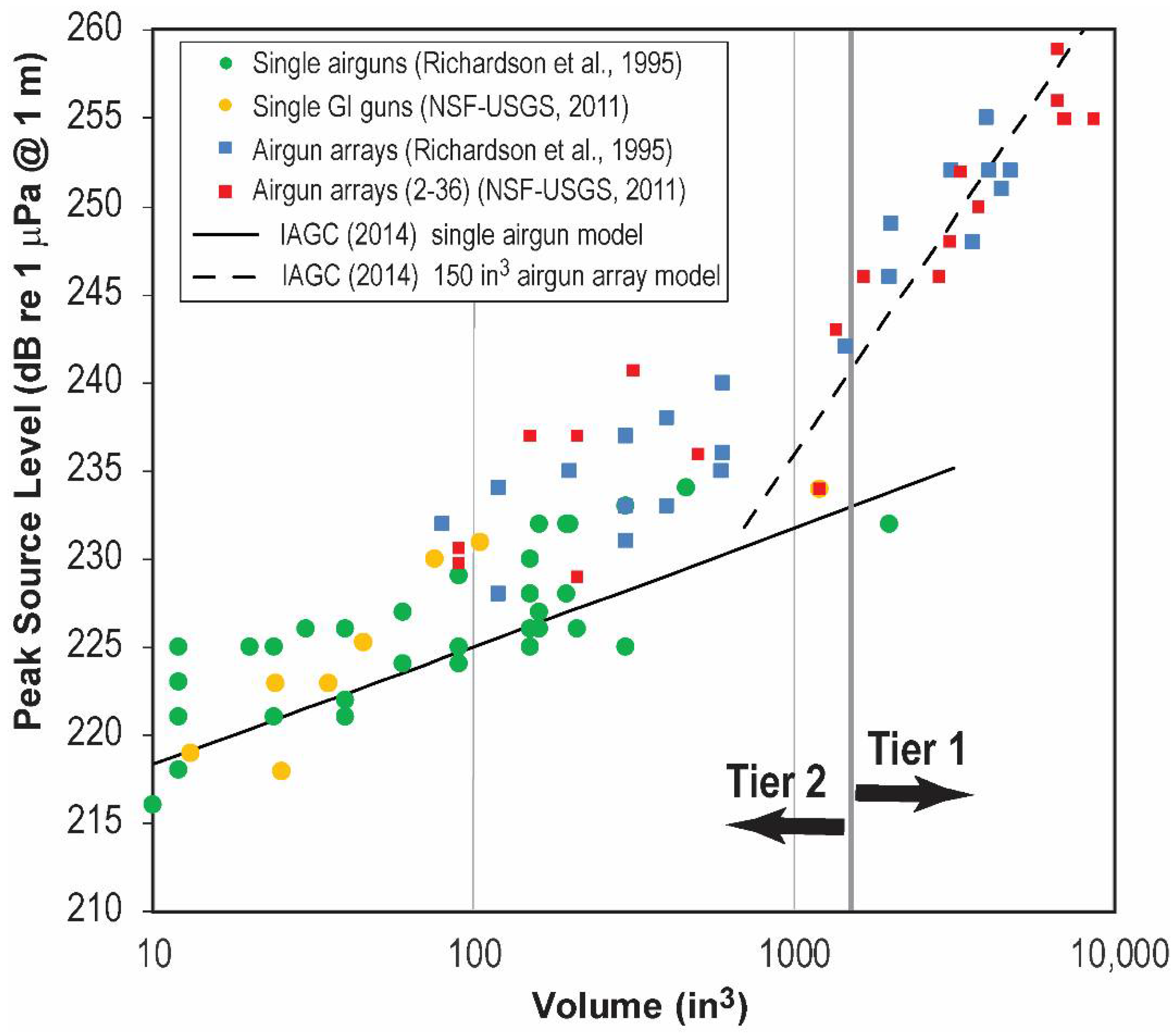
3.1. Airgun Categories

We first focus on airguns to determine if there is a natural division between different configurations used for airgun surveys and their potential impact on marine species. Figure 3 shows a compilation of measured and modeled peak SL data for single airguns and arrays. Empirical data are from a compilation by [24] and a Programmatic Environmental Impact Statement prepared for marine seismic research conducted by two U.S. federal research agencies [25], and the models are from [26]. As noted in Section 2.1, peak SL is a more consistent metric than SL for characterizing single airguns or airgun arrays because determining peak SL does not require the wavelet pulse duration to be estimated or measured. Note that peak SL is referenced to a distance of one meter from a hypothetical point source through calculation, not measurement (e.g., [52]). In Figure 3, the relationship between peak SL and total volume differs when considering single airguns and arrays. From this relationship, we designate an airgun/airgun array with a total volume of ~1500 in³ as the transition between low/intermediate energy (<1500 in³) surveys to high energy (>1500 in³ or greater than 12 airguns) surveys.

3.2. Categorization of Non-Airgun, Non-Continuous Marine Acoustic Sources

Next, we evaluate a suite of widely used HRG, oceanographic, and communication/tracking sources described in Table 1. SL is only one of several characteristics to consider when determining the impact of these sources on marine animals, but is an important starting point for the analysis. Figure 4 compiles SL data on a wide range of non-airgun marine acoustic sources, with most HRG data collected by [8] and later summarized by [53]. These studies report on a sound source verification experiment conducted on a large suite of marine acoustic sources using calibrated hydrophones to record the signals. The experimental data were acquired under controlled conditions in test tanks at the Naval Undersea Warfare Center using USGS acoustic sources and with support from BOEM. Additional data were collected at a hydrophone-equipped pond managed by the USN in Leesburg, Florida. Sparker measurements, which require saltwater, and a 1 kJ boomer test were carried out in a small moonpool flooded with ocean water at the Woods Hole Oceanographic Institution. Ref. [8] is the most complete study currently available and is now frequently cited by NMFS (e.g., 86 FR 40469 [54]), USFWS (e.g., 84 FR 2 [55]), and applicants for U.S. authorizations when evaluating the potential effects of acoustic sources on marine animals. The U.S. Marine Mammal Commission (MMC) has expressed concern that inconsistent SL have sometimes been adopted for the same acoustic sources operated in the same way and that Level B harassment zones calculated using SL reported in [8] are larger than those measured during field operations [56]. With no other exhaustive, calibrated, internally consistent data set available at this time, we will rely on the SL reported by [8] throughout this paper, while acknowledging that there may be limits to the applicability of the SL results.

Additional data have been added to Figure 4 to provide a more complete overview of MBES and hull-mounted SBP sources, as well as oceanographic and communication/tracking sources. These additional data are needed due to the limited number of (typically) hull-mounted sources considered by [8] and to cover classes of sources missing from that experiment. The additional data in Figure 4 and Table 1 mostly come from manufacturers’ specifications (e.g., [23,57,58,59]) and other studies [42,62], which sometimes do not specify whether the reported SL are rms, peak, or another measure. If the SL type is unspecified, we assume it is an rms measure in Figure 4.

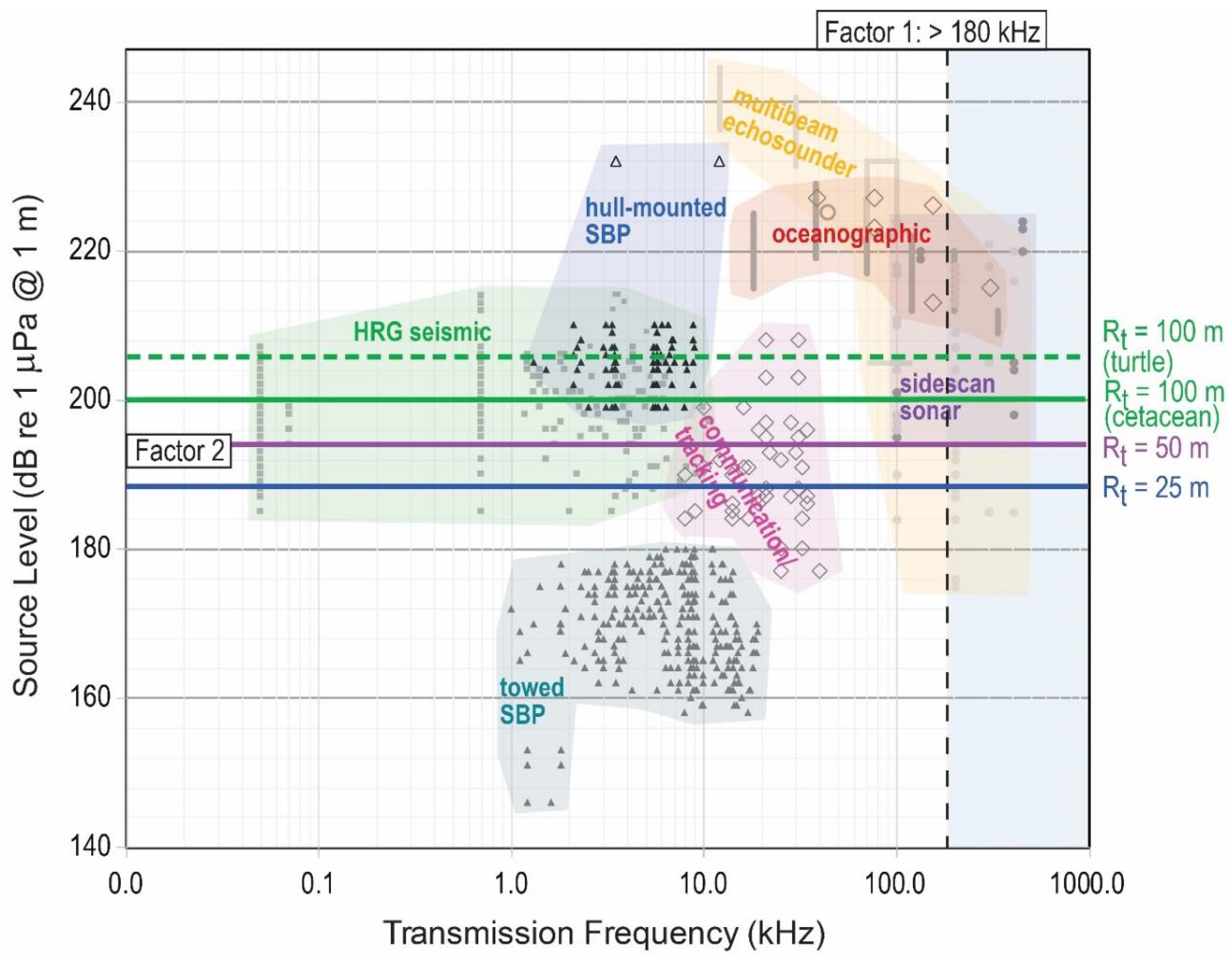
3.3. Factors for Evaluating Non-Airgun Acoustic Sources

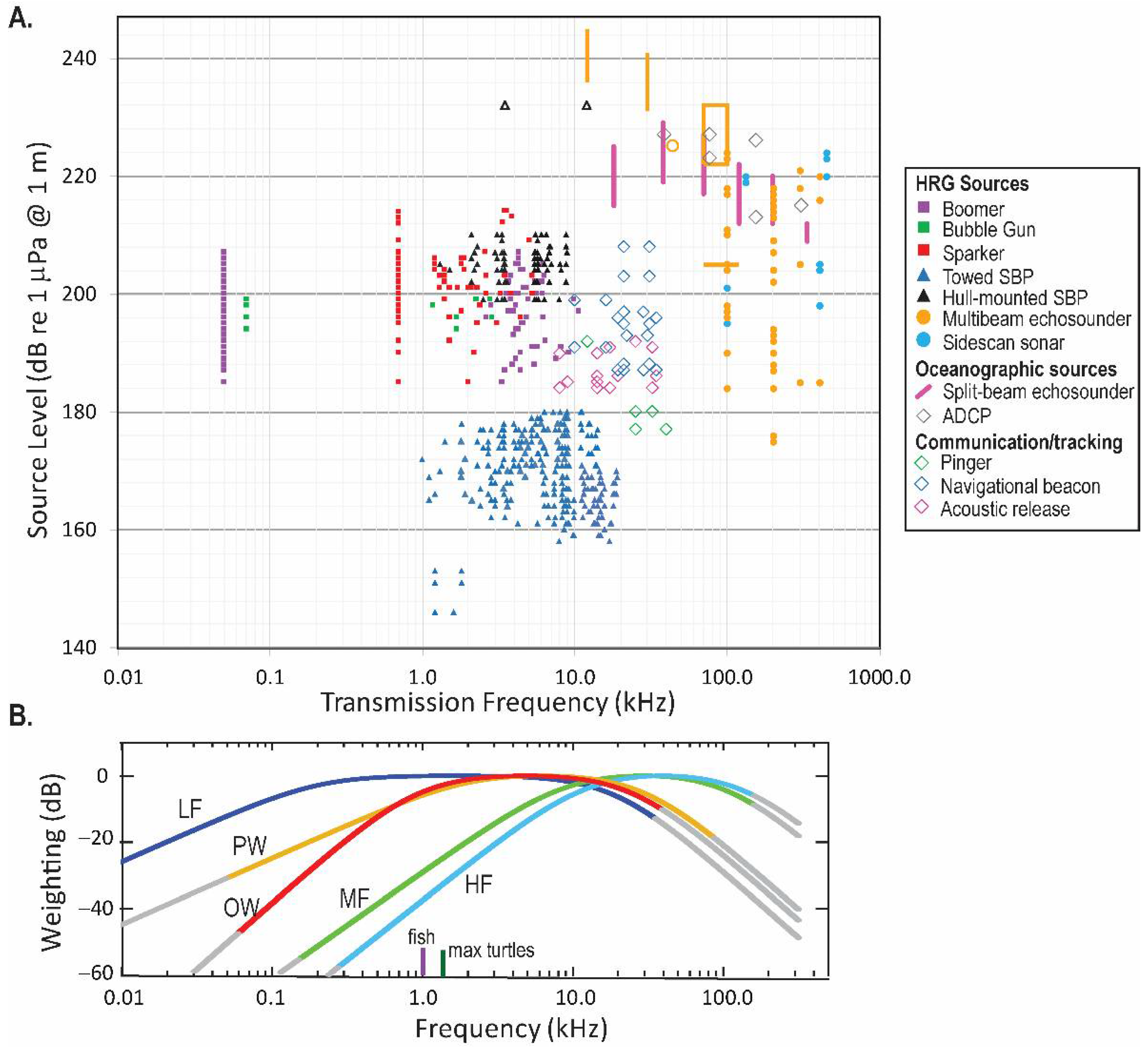
3.3.1. Factor 1: Inaudible Frequencies

The frequency of a marine acoustic source is the first factor to consider when determining the potential impact on marine species. In guidance issued by the NMFS [18], sources having transmission frequencies higher than 180 kHz are deemed inaudible by marine mammals (Figure 4B) and therefore are unlikely to result in incidental take. In Figure 5, we apply this criterion by drawing a vertical line at a transmission frequency of 180 kHz and shading higher frequencies gray. As a result, most SSS and a subset of the MBES that operate at high frequencies fall into the de minimis category. Many HRG sources (not included in Figure 5) used on AUVs, ROVs, and seafloor landers also operate at frequencies above 180 kHz because they are sensing the environment close to the vehicle or lander. To simplify Figure 5, these systems are not included, but are automatically rendered de minimis due to their operating frequencies. While sources with primary transmission frequency above the 180 kHz cutoff threshold may generate lower frequency subharmonics detectable by marine animals, the received level for these subharmonics is significantly lower than that deemed to harm an animal [63] under the current Level B incidental take criterion.

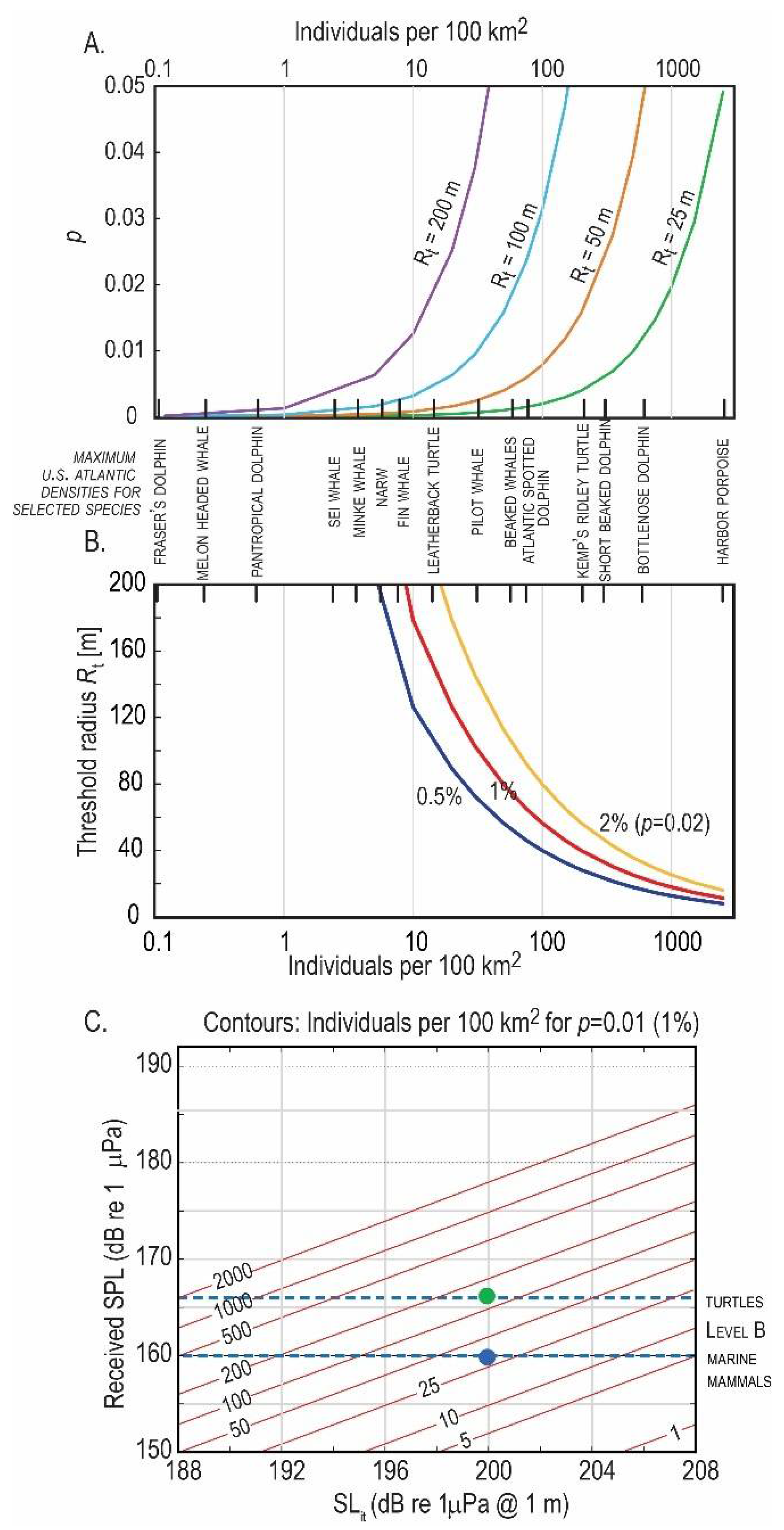
3.3.2. Factor 2: Received SPL less Than 160 dB re 1 μPa

Under the current implementation of the U.S. MMPA, assessing the possibility of Level B harassment from an intermittent acoustic source involves analyzing where received SPL exceeds 160 dB re 1 μPa (i.e., the 160 dB isopleth). When received levels are lower than this threshold, the source can be considered de minimis. As shown in Figure 5, many configurations of the towed SBP tested by [8] have SL below 160 dB re 1 μPa @ 1 m. However, the application of the received SPL criterion is too simplistic if it considers only the sound levels generated at a reference distance of 1 m.

Except for certain delphinids, which sometimes approach a stationary or moving vessel or towed sound sources, marine species generally can and often do avoid coming close to sound sources (e.g., [70]). NMFS has previously chosen a static 25 m radius around a source to describe the area that marine animals are unlikely to enter (e.g., 85 FR 14903 [64]), meaning that the 160 dB re 1 μPa criterion could be applied at this distance from the source. Instead of relying on this 25 m radius, we seek to determine an exclusion radius that has physical meaning in terms of the likelihood of ensonifying an individual animal.

Assuming that N animals are uniformly distributed at the ocean’s surface within an area A (animal density D is N/A), we define a threshold radius R_t as:

$$R_t=\sqrt{\frac{pA}{\pi N}}=\sqrt{\frac{p}{\pi D}},$$

(4)

where p is the probability p (100p is the percentage likelihood, with p = 0.01 indicating 1%) that a single animal would be within the circular area around the source. R_t is independent of the received SPL ascribed to it. Figure 6A,B applies (4) to show the relationship between R_t and p, the likelihood that a single individual will be incidentally taken in a random, uniform distribution of animals with a given density.

The results in Figure 6A,B can be used to transform R_t to an adjusted SL or SL for incidental take SL_it if the received SPL that applies to Level B harassment (SLP_B) for a given class of animals is ascribed at R_t. SL_it is the maximum SL that a source could have to produce a threshold SPL_B, currently 160 dB re 1 μPa for cetaceans in the U.S., at a distance of R_t. At the frequencies of most HRG sources (Table 1), spherical spreading dominates even for shallow water depths, leading to SL_it = SPL_B + 20log₁₀(R_it), assuming no dispersion. The NMFS criterion of R_t = 25 m for SPL_B = 160 dB re 1 μPa corresponds to SL_it of 188 dB re 1 μPa @ 1 m. This criterion would be extremely conservative for most densities of marine animals, yielding p = 0.0002 (0.02 animals within 25 m of the source or 0.02% probability of an individual being within that radius), for uniform distribution of 10 animals per 100 km². The p values are 0.002 and ~0.01 for uniform distributions of 100 and 500 animals per 100 km², respectively.

For comparison with these values, Table S1 gives the maximum density of cetaceans (Figure S1) and sea turtles (Figure S6a) in published models for U.S. mainland marine margins [65,66,67,68,71], using density grids for August when multiple months are available for a species. No ESA-protected cetacean has a density greater than 19.2 per 100 km² (humpbacks; [68]) in these models, and the maximum density for any whale species is 31.2 per 100 km² (R_t = 101 m for p = 0.01) for pilot whales on the U.S. Atlantic margin [65]. On the U.S. Pacific and Atlantic margins, some dolphin and porpoise species have maximum densities close to 300 animals per 100 km² (R_t = 32.6 m for p = 0.01) or, occasionally, much higher (Table S1). However, the 90th and 95th percentile values reported in Table S1 demonstrate that the highest densities are mostly localized, underscoring the need to consider the geographic distribution of animals when determining the likelihood of incidental take and the R_t and de minimis SL_it values. The approach outlined here is not specific to cetaceans and can also be applied to other animals with known density distributions, such as endangered sea turtles or pinnipeds. For sea turtles [66,67,71], SPL_B is typically taken as 166 dB re 1 μPa, resulting in larger SL_it than for cetaceans (Figure S7).

Using (4), animal abundances of 2, 10, 100, and 500 per 100 km² yield R_t of 398, 178, 56, and 25 m, respectively, for p = 0.01 (1% chance of a single animal being with R_t of the source). For SPL_B = 160 dB re 1 μPa Level B cetacean harassment criterion, the de minimis SL_it would range from 188 (500 animals per 100 km²) to 212 dB re 1 μPa @ 1 m (1 animal per 100 km²), as illustrated in Figure 6C. In practice, R_t and SL_it should not grow unreasonably large for very small animal densities. For example, R_t could be capped at 100 m, corresponding to p = 0.01, the density of 32 animals or fewer per 100 km². SL_it of 200 dB re 1 μPa @ 1 m for SPL_B = 160 dB re 1 μPa. Under these conditions, any source with SL_it up to 200 dB re 1 μPa @ 1 m for cetaceans or 206 dB re 1 μPa @ 1 m for turtles could be considered de minimis, as shown by the horizontal lines in Figure 5. Figure 7A shows SL_it for all U.S. mainland margins calculated for p = 0.01 using the maximum cetacean species density in each cell and spherical spreading. Except along the coast on the Atlantic and Gulf of Mexico margins and offshore southern California, SL_it is mostly 200 dB re 1 μPa @ 1 m or greater (R_t = 100 m, D = 32 animals/100 km²). If a constant R_t value were to be retained in U.S. regulatory practice for describing de minimis sources, Figure 6A and the maps in Figures S3 and S6 (cetaceans and turtles, respectively), indicate that R_t could probably be increased from 25 m to at least 40 m (the value for the density of 100 animals per 100 km² for p = 0.01), which would allow for a universal de minimis SL_it of 192 dB re 1 μPa @ 1 m.

To make the analytical formulation discussed here more applicable to different (e.g., non-uniform) distributions, Figures S4 and S5 show examples associated with calculating R_t empirically using a Monte Carlo approach based on 10⁵ realizations of animal positions for a prescribed density and probability. To provide a direct comparison to the analytical results from (4), the Supplement applies the Monte Carlo approach to animal positions drawn randomly from a uniform distribution. The strength of the Monte Carlo approach for determining R_it is its generalization to any mathematical distribution from which animal positions can be randomly chosen, including distributions that explicitly incorporate groupings or pods of animals.

As shown in Figure 5, several sources (e.g., all towed SBP, many acoustic releases and locators, and lower power levels of non-airgun impulsive sources such as sparkers and boomers tested by [8]) are within the de minimis category even if the current, R_t = 25 m (SL_it = 188 dB re 1 μPa @ 1 m) is used. If a higher threshold (200 dB re 1 μPa @ 1 m) is adopted, then even more configurations of the tested HRG seismic sources (bubble guns, sparkers, boomers), as well as most navigational beacons, would be considered de minimis based on this criterion.

These calculations have no time component and could be viewed as a discrete snapshot of the interaction of a source with a given distribution of marine animals. Moving the source through a field of stationary animals would not be an appropriate way to calculate R_t because animals generally move away from vessels before encountering an HRG source. Moving both the source and the animals requires a highly deterministic approach and would yield R_t and SL_it dependent on the motions ascribed to the animals. The simple approach we describe here is more consistent with the way in which NMFS has previously applied the R_t = 25 m criterion (e.g., 85 FR 14903 [64]).

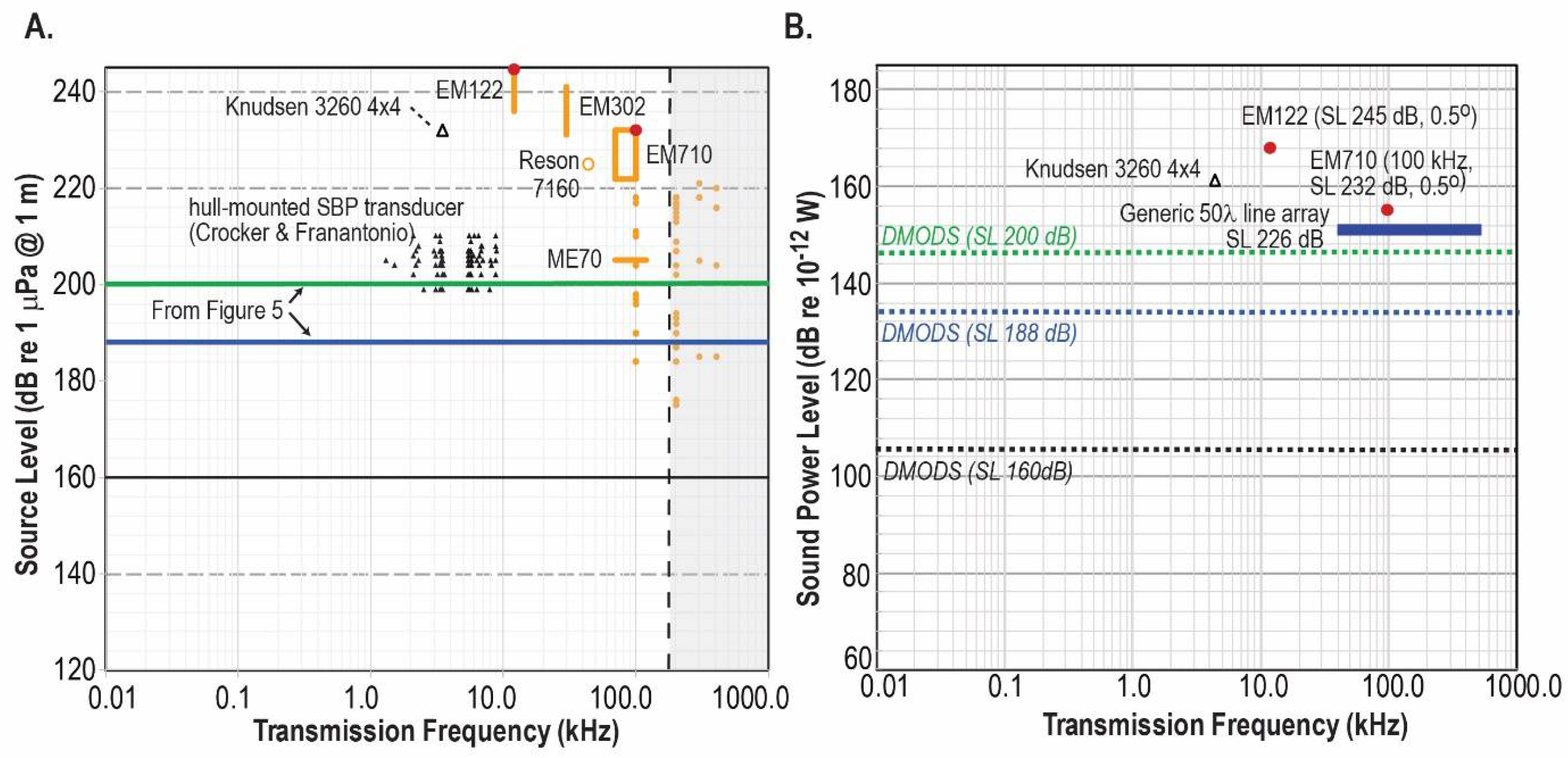
3.3.3. Factor 3: Sound Power Level (Radiated Power)

To maximize resolution and target localization, many HRG sources are designed to be highly directional. This is one justification for considering a single metric that incorporates both SL and beam pattern. As described in Section 2.1, sound power level represents such a single metric. Figure 8 compares the theoretical far-field (although never practically achieved) SL for several HRG sources to their corresponding sound power levels. As one example, the EM 122 MBES, which has one of the highest SLs for non-seismic HRG sources (245 dB re 1 μPa @ 1m [58]), has a calculated sound power level of 168 dB re 10⁻¹² W for a 0.5° beam when modeled as a 100 wavelength long by 0.2 wavelengths wide uniformly weighted line array radiating into a hemisphere below the vessel. Using the SL measure, the EM122 is 57 dB and 45 dB higher than the nominal 188 dB and 200 dB adjusted de minimis lines based on Factor 2 (Figure 5), respectively. When the directionality of the source is considered through the sound power level calculation, the EM122 would be only 34 dB and 22 dB higher than that for corresponding de minimis omnidirectional sources (DMODS; 134 dB re 10⁻¹² W and 146 dB re 10⁻¹² W) radiating into a hemisphere (Figure 8B). A similar sound power level calculation for the Knudsen 3260 4 × 4 (16-transducer) arrays operated at 3.5 kHz yields a value of 27 dB and 15 dB above the corresponding DMODS using sound pressure levels compared to 44 and 32 dB (using SL) above the 188 dB and 200 dB adjusted de minimis lines from Factor 2, respectively.

This analysis underscores that directional sources have a smaller effect than might be anticipated by considering only SL. Sound power level considerations alone do not render sources like the EM122 and the Knudsen 3260 de minimis but do bring them closer to that classification. In the future, some highly directional acoustic sources not yet invented or existing sources that are not fully considered in this paper might be shown to be de minimis based on sound power levels being less than the DMODS value for the corresponding SL_it from Factor 2.

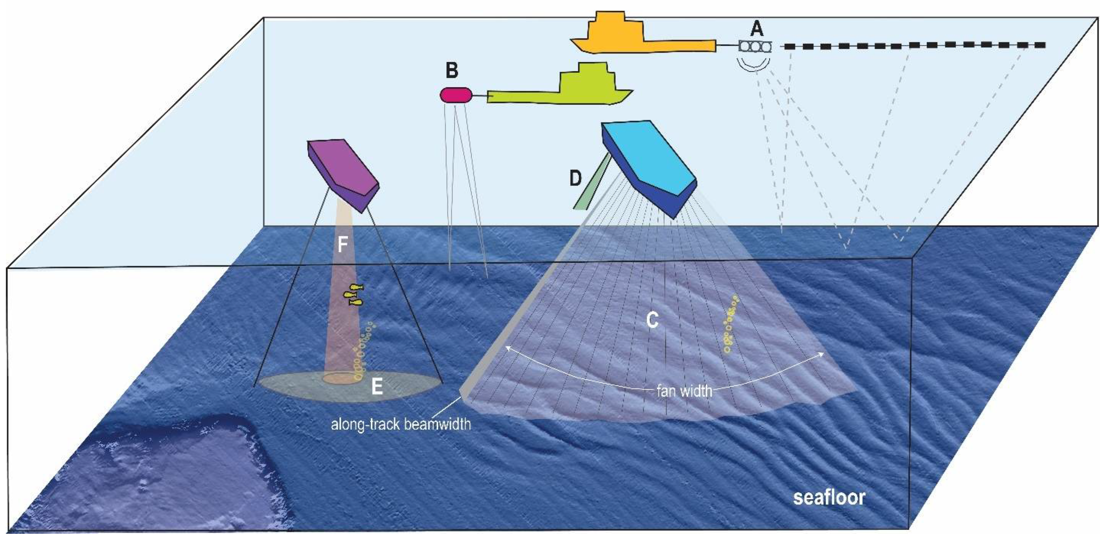
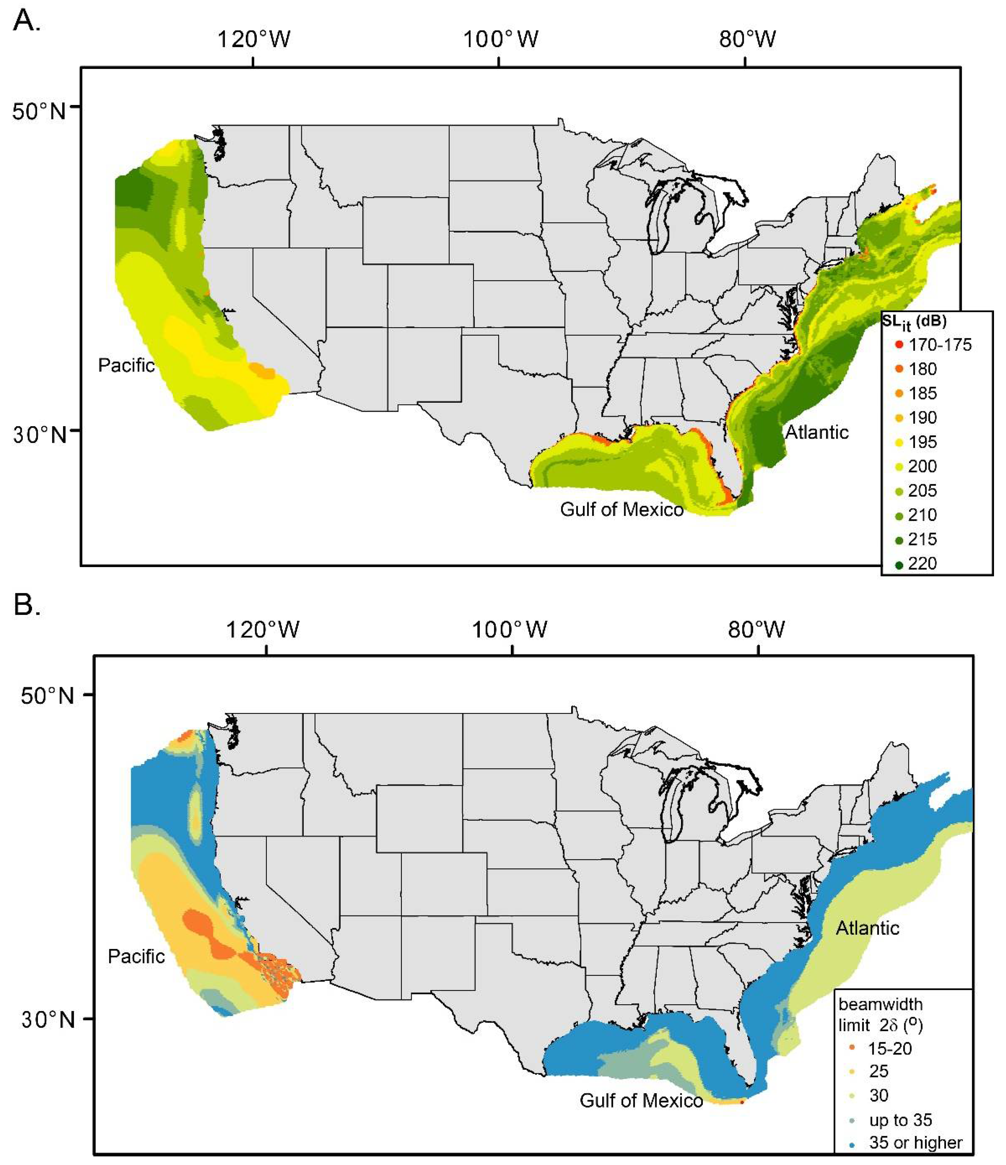
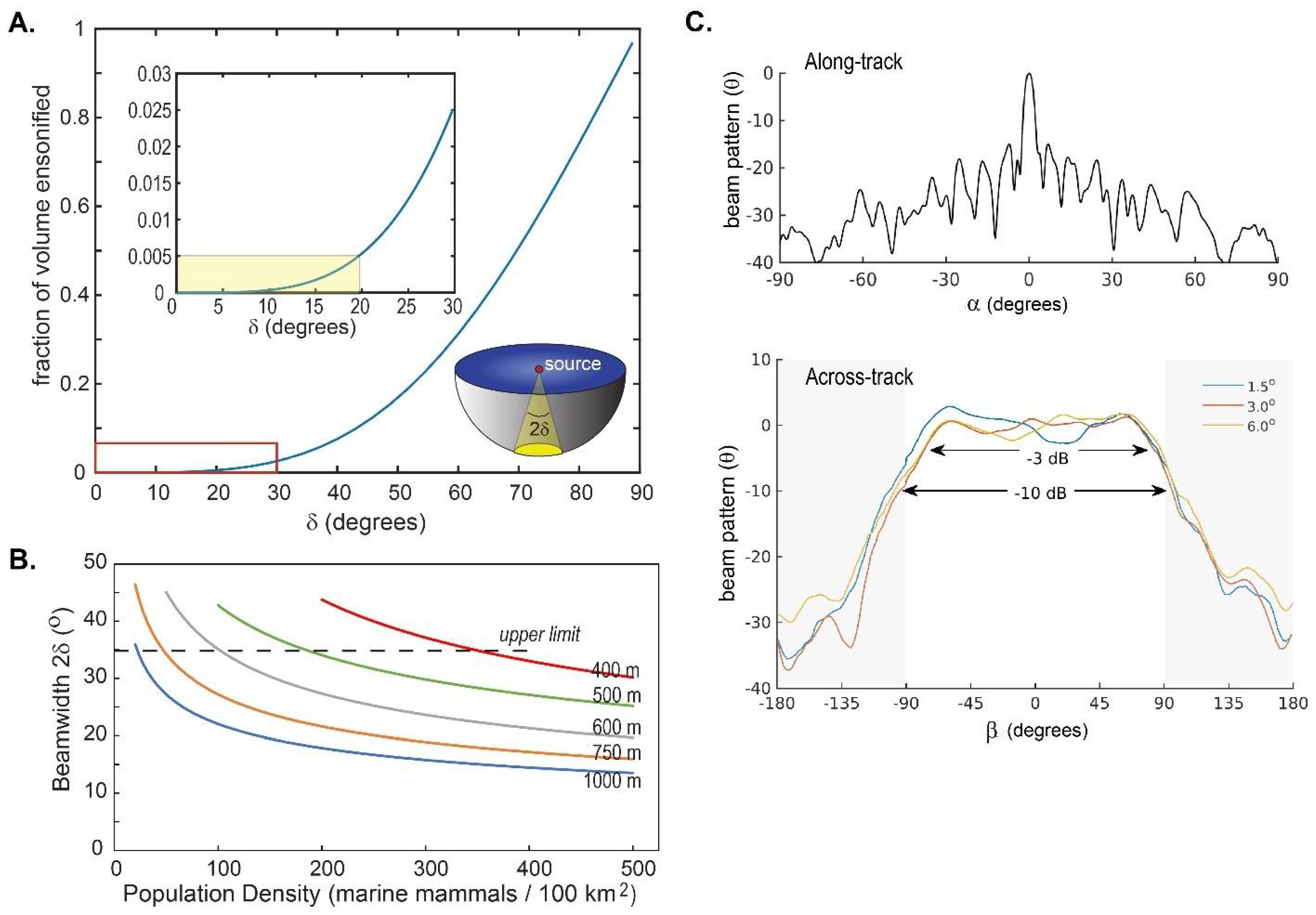
3.3.4. Factor 4: Beamwidth

Beamwidth is usually defined as the angle over which a signal emitted from a source is reduced to half its peak intensity (−3 dB from the maximum level). Thus, a 20° beamwidth indicates that sound levels are between maximum and half intensity at up to 10° on either side of the center of the beam. Increasing the beamwidth increases the ensonified volume (which has parallels to R_it, a two-dimensional measure, for Factor 2) and lowers source directivity (which is related to Factor 3). Some aspects of beamwidth, especially the three-dimensional nature of water column ensonification, should be considered independently of Factors 2 and 3 when evaluating the impact of an acoustic source and developing de minimis thresholds.

The ocean volume ensonified by an acoustic source varies non-linearly as a function of beamwidth 2δ, as shown in Figure 9A. An imaginary hemisphere of radius R centered on an acoustic source has volume ($2\pi R^3/3$). Here, R might be thought of as the distance between the source and an animal in the water column. Assuming no beam spreading, the volume of the sector corresponding to a half-beamwidth of angle δ [radians] is given by $2\pi R^3(1-\cos \delta )/3$. Thus, the ratio of the ensonified sector volume to the entire hemispheric volume is $1-\cos \delta$, an expression independent of the distance R from the source. Figure 9A shows that the fractional volume ensonified is ~0.5% of the hemisphere for δ of ~20° (when converted to degrees), which would correspond to source beamwidth up to ~40°.

To quantitatively determine how many animals are within the ensonification cone of a near-surface source, we use cetacean density models [65] for marine margins adjacent to the U.S. mainland [65,68]. Density calculations are given in terms of surface area, but the ensonification caused by an acoustic source is properly calculated as a volume. To address this, we use Monte Carlo simulations to randomly choose the x-y position of animals from a uniform distribution, as discussed above for the determination of R_t (see Supplement). Animal depths are assigned between the surface and a maximum ocean depth ranging from 400 m to 1000 m by randomly choosing from a normalized gamma distribution (Figure S8) that has most of the animals in the uppermost part of the ocean. Figure S8 also shows a sample realization for the (x, y, z) positions of 350 animals in a block 1000 m deep.

We define the beamwidth limit for a given animal density to correspond to the 2δ value for which 1% (p = 0.01) of the Monte Carlo simulations have a single animal occurring within the ensonification cone. This is similar to the threshold we used to explore possible de minimis limits for SL_it at R_t for Factor 2 (p = 0.01). We do not refer to the beamwidth limit as an incidental beamwidth limit because this metric does not include consideration of SL. An animal within the beam of a directional source is not necessarily incidentally taken because the received SPL may not exceed SPL_B, which is currently 160 dB re 1 μPa for cetaceans [19,20].

Figure 9B shows the calculated beamwidth limit as a function of animal densities as high as 500 per 100 km² for animals distributed according to the gamma function through different depth ranges, as indicated on the curves. Beamwidths below each curve (smaller beamwidths) are those for which incidental take is highly unlikely. At water depths between 400 and 1000 m (or animals known to be distributed only within these depth ranges of thicker water columns), the curves in Figure 9B can be used as a first approximation for the appropriate beamwidth limit, which is greater than 20° for densities below ~130 per 100 km² for 1000 m depth, ~250/100 km² for 750 m, and for all densities shown for shallower waters. For water depths greater than 1000 m, the 1000 m curve in Figure 9B should apply, assuming that nearly all animals are distributed in the upper 1 km of the water column. At water depths between 400 and 1000 m, the curves in Figure 9B can be used as a first approximation to the appropriate beamwidth limit. For water depths less than 400 m or animals distributed only shallower than 400 m in a thicker water column, the beamwidth limit will exceed 30° for the full range of densities plotted. To avoid the beamwidth limit growing unreasonably large in shallower waters, we suggest 35° as the de minimis beamwidth threshold for all water depths less than 400 m. Figure 7B shows beamwidth limits calculated for the U.S. mainland marine margins using published marine mammal density models and the approach outlined here.

MBES is an HRG source for which beamwidth is routinely discussed, and specifications for several frequently used MBES systems describe beamwidths as small as 0.5° or 1° and up to 6°. Note that this measure describes beamwidth in the along-track direction (direction of vessel movement; Figure 2 and Figure 8c). Across the track (athwartships), the MBES transmits a wide fan composed of many beams (Figure 2 and Figure 8). In Figure 8 the measured waveforms are from [8] for the along- and across-track directions using an intermediate frequency (100 kHz) MBES system (Reson 7111) held vertically in the water column. Neglecting variations along the center of the wide fan, Figure 9C shows that the across-track SLs fall by 3 dB at ±60°, yielding ~120° as the fan width perpendicular to the ship’s motion. This value is nearly invariant for along-track beamwidths of 1.5° to 6°.

MBES clearly do not have narrow beamwidth that renders them de minimis when both the along-track and across-track dimensions are considered, and SSS have similar geometries, although with smaller ~50° fan widths. However, other acoustic sources, particularly those that image or evaluate the water column, have nominal beamwidths less than the smallest value (2δ = 20°) mentioned above for high animal densities. For example, SBES EK60/80 transducers at frequencies of 38 kHz and higher have 7° (conical) beamwidth, while the lowest frequency (18 kHz) transducer has a beamwidth of 11°. Common Teledyne ADCPs have up to four beams, usually with a beamwidth of 8° except for the Workhorse 75 kHz, with a beamwidth of 11.8° [22]. On the basis of beamwidth alone, EK60/80 systems and ADCPs could be considered de minimis for operations at all water depths. We do not evaluate parametric SBPs in this study, but NMFS has previously indicated that the beamwidth for at least one system [15] is small enough that its use is unlikely to result in incidental take (85 FR 14903 [64]).

In Figure 7B, the beamwidth limit is 35° or greater on most of the U.S. Atlantic and northern Gulf of Mexico margins for the density models of [65] and also offshore Washington and Oregon on the U.S. Pacific margin based on the density models of [68], which use a different methodology than [65]. Overall, the smallest (most conservative) beamwidth limit discussed in the previous paragraph (2δ = 20°) is too restrictive for U.S. mainland marine margins. Depending on the beamwidth limit adopted as the de minimis threshold, even a directional source such as the Knudsen 3260 hull-mounted SBP, which has a nominal beamwidth of ~30°, could be considered de minimis for most water depths and marine mammal densities.

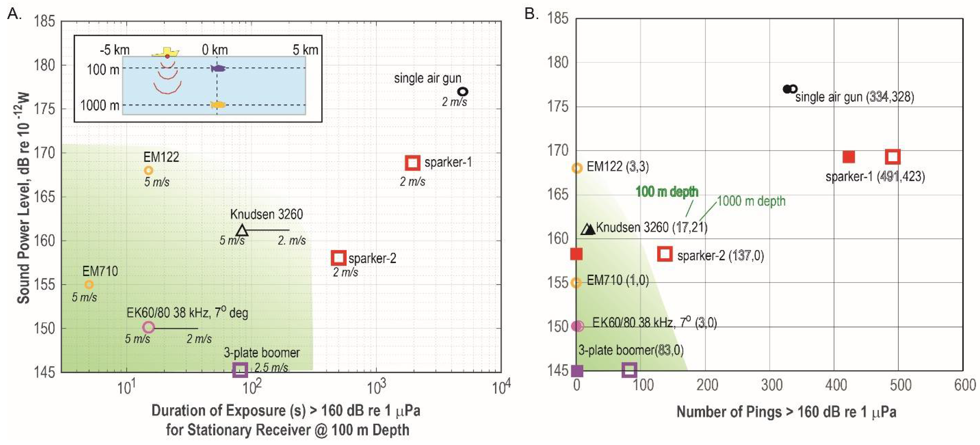
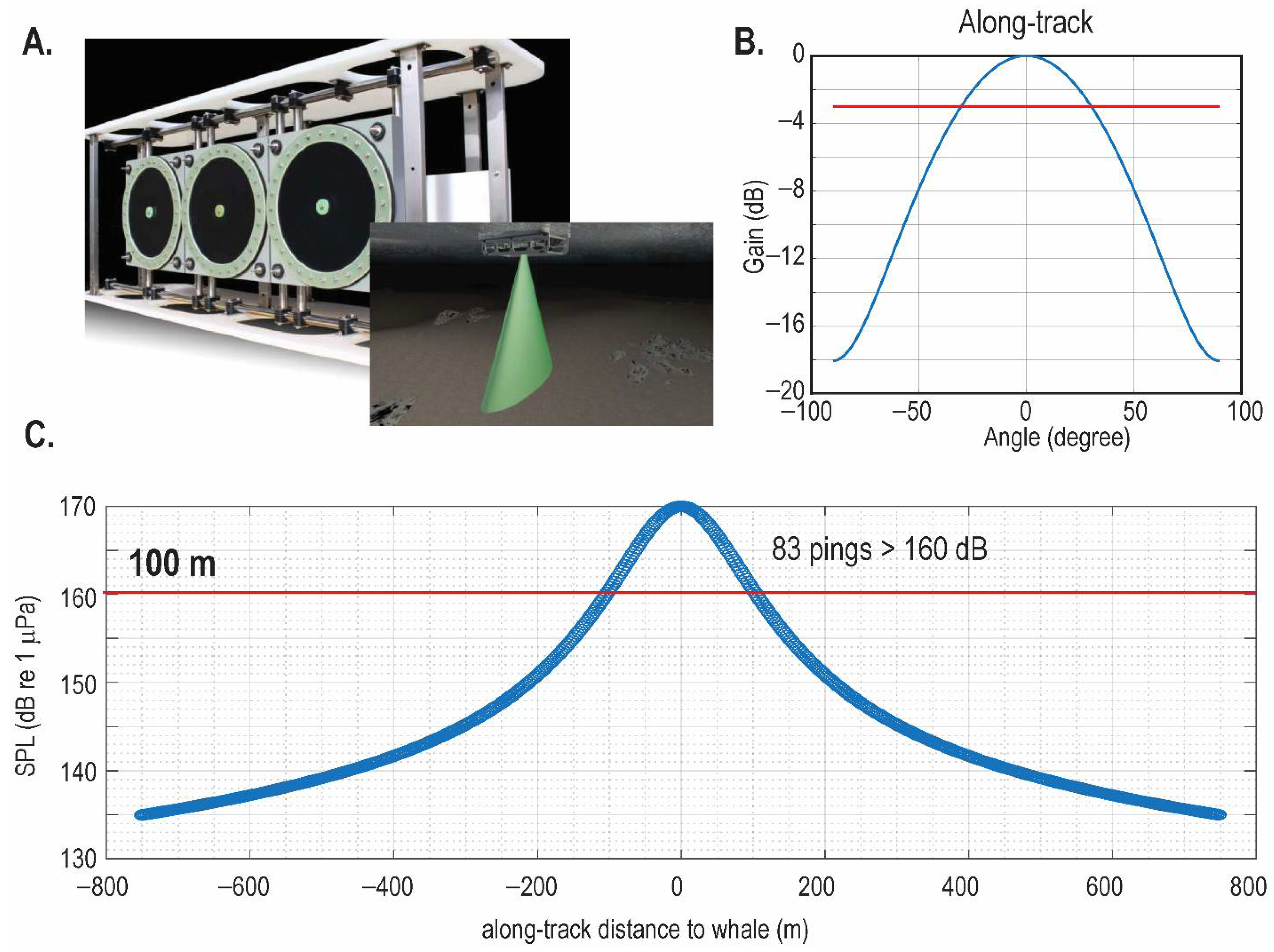
3.3.5. Factor 5: Degree of Exposure

The final factor that we use to evaluate the effects of non-impulsive acoustic sources on marine mammals is the “degree of exposure”. Whereas the first four factors (Section 3.3.1,Section 3.3.2,Section 3.3.3,Section 3.3.4) are based on a single metric (e.g., transmission frequency, beamwidth) or a blended metric that combines two parameters (e.g., radiated power), the degree of exposure criterion is a composite factor that depends on aspects of the source (source level and directivity, pulse characteristics), the vessel (speed), and the animal (position relative to the source, total duration of received sound above a defined threshold). Qualitatively, lower source levels, greater source directivity, faster vessel speeds, and an animal’s greater distance from the source (e.g., [70]) are usually associated with a lower degree of exposure. Pulse rate and pulse length, which are not explicitly mentioned in these qualitative considerations, require deeper examination, as does the total duration of exposure.

For an intermittent HRG source, the user typically selects the pulse length, which is usually on the order of 10⁻¹ to 10¹ ms, and the pulse rate, which sets the time between the transmission of consecutive pulses (repetition rate). In some cases, the choice of pulse length (ping duration) may depend on water depth or the desired data resolution. Generally, smaller pulse lengths can provide higher resolution, but longer pulses may be needed to penetrate to greater ocean depths. For most instruments, pulse lengths are limited by the physics of the HRG source and the instrument’s mode of operation. For example, choosing FM instead of CW mode for a MBES provides access to a different range of available pulse lengths. For a moving source, the pulse repetition rate (also called ping rate) is typically chosen to provide the desired lateral resolution and sufficient overlap for measurement or image and to ensure the sufficient time between consecutive pulses for the return signal to be received and processed. The duty cycle for a given source configuration is the ratio of the user-chosen pulse length (duration) to the ping rate, and most HRG sources can be operated with a range of duty cycles. A low duty cycle means longer periods of silence between pulses, which may in turn reduce the potential of a source to lead to incidental take.

For the receiver (animal side), we define ping exposure as the maximum number of pings exceeding SPL of 160 dB re 1 μPa that a stationary animal could receive. Exposure duration is the total time over which those pings could be received and includes the periods of silence between pings. The exposure duration is therefore a function of ping rate, but not pulse length. Thus, animals exposed to 20 pings exceeding 160 dB re 1 μPa over a 100 s period (5 s ping rate) and 100 pings above that same threshold over a 100 s period (1 s ping rate) would have the same exposure duration.

In the U.S., no quantitative precedents exist for a de minimis degree of exposure. On the source side, many HRG sources have been described in terms of “low” duty cycles or “short” pulse lengths and have been deemed to have few or negligible effects on marine animals even though the criteria have not been quantitatively defined (e.g., 82 FR 19521, 85 FR 72316 [72,73]). On the receiver (animal) side, there is likewise no threshold for the number of pulses at a given SPL that would constitute incidental harassment. There has also been little consideration given to the speed of moving sources relative to animals. Faster vessels clear an area more rapidly (e.g., [70,74]), leading to lower exposures in most cases, even while the risk of a vessel strike or entanglement in towed equipment could be greater for higher vessel speeds.

Defining ranges for all the parameters that would render a given survey de minimis based on the degree of exposure is beyond the scope of this study. Here, we focus on source characteristics (source level and directivity, which combine as radiated power or sound power level in Factor 4), exposure duration for a fixed vessel speed and fixed receiver (animal) depth in the water column, and the number of pings received above SPL_B = 160 dB re 1 μPa and compare key HRG sources to determine if there are natural qualitative splits among the sources (e.g., low or high degree of exposure). Figure 10 summarizes the sound power level from various sources operated at maximum SL (except Sparker-2), at the position of a stationary animal (receiver) at water depths of 100 m and 1000 m along a shiptrack extending from −5 km to 5 km relative to the animal, as shown in the inset diagram. To generate the results in Figure 10, we use simple models that account for the key features of an acoustic source (e.g., SL, frequency, beam pattern) and sound transmission in the water column instead of more complex models that provide very accurate depictions of the sound emitted by a source and its propagation. The models we use should generally be more conservative (i.e., generating larger isopleths, higher SPL, more received pings) than more sophisticated models.

Based on both exposure duration and the number of pings received above 160 dB re 1 μPa, clear differences emerge in Figure 10 between larger, impulsive, omnidirectional sources (e.g., Sparker-1 operated at 6 kJ; a single airgun) compared to HRG sources that are lower powered and have varying directionality and impulsivity characteristics (e.g., MBES, EK60/80, hull-mounted SBP, three-plate boomer, and smaller sparker, such as Sparker 2 operated at 700 J). The exposure durations shown in Figure 10A are based on specific ping rates and characteristic vessel speeds, but the durations are easily adapted to different vessel speeds (or ping rates) through multiplicative factors. For example, if the model shown in Figure 10 is formulated with a source moving at ~9.7 knots (5 m/s), but the source is instead used on a vessel transiting at 2 m/s, then the exposure duration would increase by 2.5 times. In a similar way, if the ping rate used for Figure 10 were 0.5 s, but the source is actually operated with a 1 s ping rate in the field, then the exposure duration and the number of pings greater than 160 dB re 1 μPa (Figure 10B) would be halved.

Although we do not define quantitative criteria for a degree of exposure metric corresponding to HRG sources unlikely to lead to incidental take, the green shading in Figure 10 groups together non-seismic HRG sources not rendered de minimis by Factors 1 through 4 (e.g., hull-mounted SBP, MBES), EK60/80 (de minimis based on Factor 4), and a specific seismic HRG system (e.g., three-plate boomer) as potential de minimis sources. The low-powered Sparker-2 would be just outside this de minimis group. Given the importance of the degree of exposure criterion in rendering de minimis a range of HRG sources, we provide more detail for some classes of sources below.

Multibeam echosounders. Calculations for the EM122, the most powerful and lowest frequency MBES commonly used in the U.S. federal research fleet, should provide the most conservative (worst case) assessment of the degree of animal exposure to MBES sounds. Figure 11 shows the modeled SPL received by a stationary animal at depths of 1000 m and 100 m as a vessel moving at 5 m/s (9.7 knots) runs an EM122 at an SL of 245 dB re 1 μPa @ 1m with 0.5° (along-track) beamwidth along a 10 km trackline with the geometry shown in the inset to Figure 10A. The simulated EM122 uses a uniformly weighted line array that overestimates the impact of sidelobes in the along-track direction, and more sophisticated published models show that the array-shading used by the EM122 actually lowers the sidelobes by ~15 dB [75]. The simple model used here also does not include so-called transmit sectors, where the transmit fan beam is transmitted as separate segments of the entire fan (see [75] for details). Including transmit sectors is not likely to affect the calculated SPL, but could increase perceived pulse length.

In Figure 11, three pings (pulse exposure) exceed the SPL threshold of 160 dB re 1 µPa (e.g., Figure 10B) for EM122 15 ms (CW) pulses repeated every 5 s, and the highest received SPLs are 195 dB and 183 dB re 1 µPa for the animals at 100 and 1000 m depth, respectively. For the sake of comparison, we also plot the DMODS for which SPL reaches 160 dB re 1 µPa within 25 m of the source (related to Factor 2, with R_it = 25 m). The EM122 calculation is for single swath mode. In normal operations, a 0.5° EM122 would be operated in dual swath mode, transmitting two 15 ms pings (one each pitched slightly forward and backward) separated by a few hundred milliseconds. This effectively doubles the number of pings (from 3 to 6) that could exceed 160 dB re 1 µPa, although a stationary animal could receive the highest SPL for only a single of any two-ping pair.

Changes in along-track beamwidth, which was taken as 0.5° in Figure 11, do affect the SPLs. Larger beamwidth widens the along-track zone where the SPL is near the highest values, but also lowers the system’s SL and thus received SPL values, by as much as 9 dB [58]. Thus, a few additional pings may exceed the 160 dB re 1 µPa threshold for larger beamwidth, but most pings will be at a lower SPL. Repeating the calculation for a 2° EM122 with an SL of 236 dB re 1 μPa @ 1m (with other parameters the same) yields SPL for the five highest pings of 196 dB (1 ping), 160 dB (2), and 159 dB (2) re 1 μPa at 100 m depth and 175 dB (1), 168 dB (2), and 160 (2) re 1 μPa at 1000 m depth.

A stationary animal has only a small chance of being directly affected by one of the highest SPL pings. With pings transmitted every 5 s, the ship covers a 25 m distance in the time necessary to transmit a single 0.015 s duration ping, which endures for 0.075 m of the ship track in the single swath case. An animal at 100 m water depth has only a 3.5% chance of being within the 0.87 m along-track zone affected by the maximum SPL from a given ping for a 0.5° swath (14% chance for a 3.5 m zone for the 2° swath).

Next, we consider the duration of the animal’s exposure. In the unlikely event that an animal received all three pings exceeding SPL of 160 dB re 1 µPa in the model shown in Figure 11, the exposure duration would be 15 s for the single swath CW mode, with the sound transmitted only for 0.045 s of that time (quiet period of 14.955 s out of 15 s). For single swath FM mode, which is used at water depths greater than ~2000 m and is associated with a maximum pulse length of ~100 ms [57], the exposure duration remains 15 s, but the sound would be transmitted for 0.3 s of that time (quiet period of 14.7 s). Here we begin reporting the amount of time that the sound is “on” to inform later discussions of the duty cycle and auditory integration time.

Multibeam data are often acquired along adjacent tracklines, spaced so that the swaths completely cover the seafloor. The EM122 can usually provide high-quality data for swaths ~130° wide or 65° on either side of the ship’s center line. This value is smaller than those reported in the specifications for various systems because data collected from the outermost beams can be poor due to uncertainties, such as those related to sound refraction through the water column. Thus, researchers typically overlap adjacent swaths during surveys. For water 1000 m and 2000 m deep, the ±65° swath translates to a swath width on the seafloor of ~4.3 km and ~8.6 km, respectively. Calculating the slant range R_s at which the SPL is reduced to 160 dB re 1 μPa from $SPL=SL-20{\log }_{10}{R}_s-a{R}_s$, assuming SL of 245 dB re 1 μPa @ 1 m [58], yields ~6.5 km. A stationary animal would generally receive pings from only two adjacent tracklines, regardless of water depth. Using operational rules of thumb, if tracklines were spaced 3.5 km apart, as would be the case for a water depth of ~1167 m, and if the animal were directly beneath the vessel on the initial trackline, the animal would receive three additional pings exceeding 160 dB re 1 μPa (six additional pings in dual swath mode). For tracklines 7 km apart, corresponding to a water depth of 2333 m, the animal would receive one additional ping exceeding the threshold if the animal were directly beneath the vessel for the first swath and two additional pings if the animal were at the edge of the swath during the first pass of the vessel.

For the EM122 dual swath cases discussed here, a stationary animal would receive significantly fewer than 15 pings exceeding 160 dB re 1 μPa, assuming the EM122 is operating in dual swath mode on adjacent tracklines. The total duration of 15 pings for CW mode is 75 s, of which 0.225 s includes the 15 transmitted pulses at 0.015 s each. For a 40 ms long FM pulse, the maximum exposure duration would still be 75 s, of which a total of 0.6 s would include pulse transmission. The 9.7 knot (5 m/s) vessel speed used here is typical for surveys on global class vessels that are equipped with EM122 and similar low-frequency, deepwater MBES. A slower speed would proportionally increase the number of pulses above the threshold.

Even in the worst-case scenario for MBES systems—lowest operational frequency, highest source levels, largest along-track beamwidth, and stationary animal located only 100 m below the ship—the combination of factors that make up the degree of exposure (radiated power; exposure duration; the number of pings exceeding the threshold) indicate that MBES systems have such minimal impact that they are unlikely to result in incidental take and could be considered de minimis. For higher frequency MBES, which have greater sound absorption in the water column, and for MBES with lower SL, the SPL would be lower and the degree of exposure even smaller.

Hull-mounted SBP. Hull-mounted SBP sources such as the Knudsen 3260 can also be shown to be de minimis based on a degree of exposure criteria (Figure 10). We earlier considered near-surface towed SBP sources like those tested by [8] and determined that they met a de minimis criterion based on Factor 2. This section therefore focuses only on hull-mounted SBP, which generally use higher power levels to penetrate more deeply beneath the seafloor.

Using the Knudsen 3260 as an example of a hull-mounted SBP, a typical configuration on larger ships is an array of 16 transducers arranged in a square grouping with four per side. SL for one transducer is 208 dB re 1 μPa @ 1 m, leading to a calculated SL of 208 dB +20log₁₀(16) = 232 dB re 1 μPa @ 1 m for all 16 transducers under the assumption that all sources add coherently (i.e., perfectly in phase). Values as low as 229 dB re 1 μPa @ 1 m may be more reasonable based on extrapolation of the data in [8], but we apply the higher 232 dB value in the modeling as a worst-case scenario.

The transmission pattern for non-parametric hull-mounted SBPs is a cone directly beneath the vessel. The modeled SPL pattern for Knudsen 3260 4 × 4 system pinging every 5 s (coordinated with the MBES) at 4.5 kHz is shown in Figure 12A. The model includes near-field effects and absorption of 0.29 dB/km and uses a pulse length of 64 ms (duty cycle ~1.3%), which is the longest available, but also only infrequently used in field operations. The largest SPL is directly beneath the source, and 160 dB re 1 μPa can be received beneath the source in a cone that expands with depth, but also in the side-lobes. As shown in Figure 12B,C, a stationary animal 100 m below the water’s surface could experience up to 17 pings exceeding SPL of 160 dB re 1 μPa (exposure duration 85 s, with a total of ~1.1 s of active sound transmission and nearly 84 s of quiet). An animal at 1000 m depth could receive 21 pings above the threshold value (exposure duration 105 s) with a total of 1.34 s of active sound transmission.

These calculations were performed at the maximum SL for the transducer array. In practice, the Knudsen 3260 has selectable power levels, and setting the power level too high for a given water depth and seafloor lithology produces reverberation that significantly degrades data quality. Thus, the Knudsen 3260 and similar hull-mounted, non-parametric SBPs are rarely used at the highest SL.

In contrast to MBES, SBP data are not usually acquired along closely spaced tracklines. Even if the SBP were used on adjacent tracklines simultaneously with MBES, the conical beam pattern for SBP means that a stationary animal would not receive signals from any shiptrack besides the one passing almost directly overhead.

Boomers. Towed boomer sources have a wider transmit cone, but lower SL, than hull-mounted SBP (Figure 4A). A commonly used boomer source (triple plate S-boom; [76]) employs three circular source plates arranged parallel to the shiptrack (Figure 13A), for which [8] measures a beamwidth of ~60° (Figure 13B). The pulse shape for the boomer results in a significant difference between SL and peak SL, beyond those associated with similar sources (e.g., sparkers). To be conservative, the three-plate boomer source is modeled using SL of 210 dB re 1 μPa @ 1 m [8]. This number represents an upper operational peak SL for a typical system (Figure 4) but is used here in the context of the MMPA Level B framework that considers rms SPL. The model assumes an absorption of 0.06 dB/km, vessel speed of ~4.9 knots (2.5 m/s), a ping rate of 1 s, and a ping duration of 0.6 ms, yielding a duty cycle less than 1%.

The results shown in Figure 13C give the SPL at 100 m below the source. For spherical spreading, transmission loss at this short distance would be 40 dB, meaning that SPL should be ~170 dB re 1 μPa at the center of the beam. The total number of pings (pulse exposure) above the 160 dB re 1 μPa threshold would be 83 for an animal 100 m below the source, falling to 0 pings at greater than 320 m depth and reaching a maximum of 91 pings (exposure duration 91 s with active sound transmission for ~0.054 s and quiet for 90.946 s) between 55–80 m. The three-plate boomer has radiated power lower than any other source we consider (145 dB re 10⁻¹² W; Figure 10) and clearly groups with other sources that have small degrees of exposure. Thus, this common three-plate boomer configuration is also unlikely to lead to incidental take and should be considered de minimis.

Like hull-mounted SBPs, boomers are also generally not operated on adjacent swaths to achieve full subseafloor coverage. Even if a boomer with the characteristics described here were used simultaneously with a MBES conducting swath mapping, the boomer’s conical transmission pattern ensures that high SPL pulses would not be received on adjacent swaths. This analysis does not consider single- or dual-plate boomers, which have different transmission patterns and SL.

Oceanographic Acoustic Sources. Some SBES and ADCP sources have frequencies greater than 180 kHz, rendering them de minimis under Factor 1. We also discussed these sources in our consideration of Factor 4 (beamwidth), noting that the beamwidths of common SBES (e.g., EK60/80) and ADCP instruments are small enough for these sources to be considered de minimis. Degree of exposure arguments also supports categorizing these sources as de minimis. Figure 10 shows the degree of exposure metrics for a single 38 kHz EK60/80 transducer synchronized to the MBES and Knudsen 3260 on a vessel moving at MBES survey speeds, and the SPL model for the animal at 100 m depth is shown in Figure 14A. Note that the EK60/80 radiated power is only 150 dB re 10⁻¹² W, the second lowest of the sources considered here. Furthermore, only three pings exceed 160 dB re 1 μPa for the animal at 100 m depth and none for the animal at 1000 m (Table S2). In all of the scenarios considered here, the EK60/80 would be grouped with other sources that have a low degree of exposure and that are unlikely to lead to incidental take and therefore deemed de minimis.

ADCPs, which are considered de minimis based on Factor 4, also have a low degree of exposure. As noted above, many modern ADCPs use four narrow (~8°) beams angled away from each other at 20–30°. This geometry means that an animal could not simultaneously be within two or more beams during a single transmit pulse. For Teledyne Ocean Observer and Workhorse ADCPs at 38, 75, or 150 kHz frequency, the pulse duration ranges from 11 to 37 ms at a repetition interval of 1 to 3 s [59], corresponding to the maximum duty cycle of 3.5%. Even if an animal were to receive several pulses as a vessel passes by, the duration of the exposure and number of pings received would place these sources within the de minimis groupings in Figure 10.

3.4. Uncategorized Sources

As summarized in

Table 2. Factors that render some HRG marine acoustic sources de minimis.

DE MINIMIS FACTORS DEFINED HERE
	1: Transmission Frequency b	2: Threshold take Radius c	3: Radiated Power d	4: Beamwidth Limit e	5: Degree of Exposure f	NMFS Precedent g
1-, 2-plate Boomer a		Not evaluated
3-plate Boomer a		• (Lowest powered)			•
Sparker a		• (Lowest powered)
Bubble Gun a	Not evaluated
Marine Vibrators a	Not evaluated
Subbottom profiler (SBP; hull-mounted, non-parametric)				•	•
SBP (towed, non-parametric, for versions evaluated here)		•
SBP (parametric)	Not evaluated					•
Multibeam Echosounder (MBES)	• (Some)				•
Sidescan sonar (SSS)	• (Some)				•
Split-beam Echosounder (SBES)	• (Some)			•	•
Acoustic Doppler Current Profiler (ADCP)				•	•
Pingers (acoustic locators)		•			•
Acoustic releases		• (Most)			•
Underwater navigation		• (Some)			• (Some)	•

^a Seismic sources (separate source and receiver). ^b Section 3.3.1. Transmission frequency of 180 kHz or higher renders a source de minimis. ^c Section 3.3.2. We apply the current SEL_B for cetaceans (160 dB re 1 μPa isopleth) at the threshold radius R_t as a de minimis measure for 1% or lower probability of ensonifying a single animal based on individual species densities. ^d Section 3.3.3. Additionally called sound power level when reported in decibels. Radiated power accounts for SL and source directionality. No sources considered here are rendered de minimis through application of radiated power, but future acoustic sources could be. ^e Section 3.3.4. Beamwidth less than 20° is de minimis for all water depths and animal densities. For much of U.S. marine margins, beamwidth of even 35° would be de minimis given published marine animal densities (Figure 7B). ^f Section 3.3.5. Degree of exposure combines radiated power, duration of exposure to SPL > 160 dB re 1 μPa, how many pings are received above this threshold, and other factors. We do not propose bounds for these parameters but do identify sources that are generally associated with a low degree of exposure for the conservative cases considered here (Figure 10). ^g Parametric SBP are placed in the de minimis category based on precedents set by U.S. regulators (85 FR 14903, 85 FR 26941, 86 FR 8495 [64,77,78]). Some navigational/tracking acoustics have previously been deemed unlikely to result in incidental take (85 FR 30933 [79]).

, most HRG and oceanographic acoustic sources are unlikely to result in incidental take of marine mammals based on the factors that we consider above. This section focuses on sources that have not been explicitly considered above, as well as those that do not fit the de minimis criteria we have outlined or for which too little information is available to assess the sources.

Communication/Tracking Devices (locators and transponders). Most of the acoustic sources discussed in this paper are normally deployed on or from moving ships or robotic vehicles. For pingers and transponders, either the transmitter or receiver and sometimes both may be stationary or moving at slow speeds, and the sound source is more often within the water column as opposed to near the ocean’s surface. The stationary or slow-moving nature of the source could mean that the same part of the water column is repeatedly ensonified, but usually not for a period longer than hours or a few days during active research or survey operations.

Many pingers and transponders can be rendered de minimis based on their SL (Figure 5). Depending on the criterion adopted for Factor 2, many non-navigational devices plotted in Figure 4 and Figure 5 could be in the de minimis category. Some of these devices have directionality, and their beamwidths could render them de minimis based on Factor 4. Even when they are omnidirectional, devices such as acoustic releases operate for very brief periods, and animals would not be expected to receive multiple pings above the 160 dB re 1 μPa threshold.

Instruments in this category with SL greater than ~210 dB re 1 μPa @ 1 m should be analyzed separately. An omnidirectional pinger with SL of 210 dB re 1 μPa @ 1 m would have a sound power level of 156 dB re 10⁻¹² W and produce 0 pings above 160 dB re 1 μPa at 1000 m range. The number of pings above the threshold for smaller distances and how those pings affect resident animals when the acoustic source is lowered into the water or is used to navigate vessels near the seafloor is the degree of exposure criteria that will affect the final categorization of such sources.

Navigational beacons and transponders, like those used for some USBL, LBL, and SBL systems, are deployed primarily on stationary gear (e.g., landers) or very slow-moving vehicles (e.g., ROVs); can have SL above 210 dB re 1 μPa @ 1 m; usually transmit at frequencies below 180 kHz; vary from omnidirectional to highly directional and may transmit horizontally near the seafloor instead of vertically (LBL). Specific navigational systems may meet de minimis criteria under Factors 1 to 5, and NMFS has determined that one USBL was unlikely to lead to incidental take (e.g., 85 FR 30933 [79]). Evaluating the likelihood of incidental take from other systems would require consideration of their unique characteristics unless these systems were uniformly deemed to be outside the regulatory framework due to their importance for the safety of vehicles and people.

Sparkers. As omnidirectional, shallow-towed HRG seismic sources transmitting at relatively low frequencies (500 Hz to 5 kHz), most sparkers lack the frequency, beamwidth, and degree of exposure characteristics to automatically meet the de minimis criteria described in Section 3.3. Ref. [8] tested sparkers operating up to 2.5 kJ (Figure 4A), but one instrument they tested could be powered at up to 12 kJ for an estimated peak SL of 232 dB re 1 μPa @ 1 m [80]. As shown in Figure 5, the very lowest powered sparker operations tested by [8] have SL small enough to render them de minimis based on some proposed Factor 2 SL_it criterion. In Figure 10, the degree of exposure arguments renders the sparker operated at 700 J (e.g., SIG ELC 820) close to the de minimis source grouping. For other sparker modes whose SLs are shown in Figure 4 and for more powerful sparkers (up to 40 kJ [12]) not tested by [8], the distance to the 160 dB isopleth is not well constrained and would vary with water depth. Based on Figure 10, a 6 kJ sparker has a degree of exposure characteristics closer to that of a single airgun than to the de minimis sources. Figure 14B shows a comparison of the SPL for two sparker configurations (sparker 1 of 6 kJ and sparker 2 of 700 J) along with the de minimis three-plate boomer. The results underscore the variations in SPL associated with these different seismic sources, but also the smaller exposure duration and number of pings above 160 dB re 1 μPa for the 700 J sparker (and three-plate boomer). Recent measurements by the USGS [81] show nearly spherical spreading of sparker signals even at 25 m water depth, meaning that the results in Figure 14B should be representative of most smaller sparker configurations. Additional field measurements are needed before sparkers can be fully evaluated in terms of the likelihood of incidental take for shallow and deepwater cases in various configurations of SL and ping rate. Restricting sparker power levels based on water depth and introducing defined mitigation and monitoring measures could ensure that many sparker operations would be unlikely to lead to incidental take.

Bubble Guns. Although a few configurations of bubble guns were tested by [8], we lack sufficient data to fully evaluate bubble gun sources in terms of the de minimis criteria described in Section 3.3. The published SLs for single, dual, and low-frequency bubbles guns are 200, 204, and 220 dB re 1 μPa @ 1 m, respectively [39,40], and [8] measures less than 200 dB re 1 μPa @ 1 m for the configurations that they tested (Figure 4). When operated at the lowest SL, bubble gun sources fall below some proposed Factor 2 SL_it thresholds (Figure 5). For higher SL, the directionality of bubble guns could mitigate some of their impacts, but too little is known about their beam pattern to fully evaluate their beamwidth (Factor 4), calculate their radiated power (Factors 3 and 5), or quantitatively assess the degree of exposure (Factor 5). Bubble guns can generate rapidly repeated (up to 8 Hz), short-duration (less than 2.4 ms) pulses, corresponding to a duty cycle of less than 2%. One hundred pings could be transmitted in less than a minute, and a ship towing a bubble gun at 5 knots (~2.6 m/s) would progress only ~150 m during that minute, underscoring the importance of accurate beam pattern information for evaluating the possibility of incidental take from this source.

Boomers. The calculations in Section 3.3 and shown in Figure 13 and Figure 14b focus on a three-plate boomer, which was found to have peak SL the same as or only 1 dB re 1 μPa @ 1 m higher than one- and two-plate configurations at 300 J or higher for the Applied Acoustics S-boom [8]. However, the three-plate boomers have the smallest along-track beamwidth (~60°) of any of the tested configurations, meaning that they have more directionality and lower radiated power. For one- and two-plate configurations, the along-track beamwidths can be 70° to greater than 90° and further analysis (modeling and/or field measurements) is needed to determine if these systems could fit any de minimis criteria. Three-plate boomers that are differently configured (e.g., higher peak SL) than the one discussed here should also be independently evaluated.

Parametric SBPs. As noted in Section 2.3.2, parametric SBPs use two discrete frequencies to construct a high-resolution image of the subsurface. These systems are not yet in widespread use in the US federal research fleet but are growing in popularity. The published SL of parametric SBPs ranges from ~200 to more than 245 dB re 1 μPa @ 1 m [14,15] for the primary frequencies. At the upper end, this SL exceeds that of typical hull-mounted non-parametric SBPs such as the Knudsen 3260 (Figure 4) although the beamwidths for the primary frequency of parametric SBPs are smaller than those of sources considered in the de minimis range in Factor 4. NMFS invokes the very small primary beamwidth of parametric SBPs (85 FR 14903; 85 FR 26941 [64,78]) and the small inferred 160 dB isopleth radius (86 FR 8495 [77]) to conclude that the likelihood of take of a marine mammal with these systems is “so low as to be discountable” (85 FR 26941 [78]). Modeling the complex beam pattern, pulse characteristics, and multiple frequencies and beamwidths of parametric SBPs is beyond the scope of this paper, but we classify parametric SBPs as de minimis based on the cited precedents established by NMFS.

Marine Vibrators. Marine vibrators (vibroseis) are experimental, non-impulsive seismic sources that have been investigated as a potential replacement for airguns, particularly for surveys in shallow water or in environmentally sensitive areas [10,82,83]. Using hydraulics or electromagnetics, vibroseis sources generate a broadband seismic signal that mimics the low-frequency characteristics of airguns and can be designed to include frequencies (~100 kHz) for higher resolution imaging, while suppressing energy at the highest frequencies (greater than ~150 kHz [10]). Compared to airguns, vibroseis sources can have lower peak energy, longer duration pulses, higher portability (no compressors needed), high tunability and repeatability, and better elimination of unwanted frequencies. Some of these factors should contribute to reduced impact on marine mammals [84] even though the long duration (seconds) of marine vibroseis signals yields high-duty cycles (shorter quiet periods between pulses). The private sector has evaluated marine vibroseis sources [10] and the resulting seismic data, but the sources are not yet used routinely. This study cannot categorize marine vibrators or make comparisons with airgun and other seismic sources, but marine vibroseis could eventually be evaluated for its impact on marine mammals using some of the criteria outlined here or new criteria not explored in this paper.

4. Discussion

4.1. Tiering of Marine Acoustic Sources

Based on the technical analysis in Section 3, we devise four tiers for acoustic sources (

Table 3. Proposed tiering of controlled active marine acoustic sources based on their impact on marine mammals. Marine vibrators are not listed here.

Category	Short Description	Example Sources
Tier 1	High-energy airgun surveys (includes GI guns)	Total airgun volume > 1500 in3 or arrays larger than 12 airguns
Tier 2	Low/intermediate energy airgun surveys (includes GI guns)	Total airgun volume < 1500 in3
Tier 3	HRG seismic sources (most)	Some sparker configurations Impulsive sources requiring further analysis: bubble gun; some 1-and 2-plate boomers
Tier 4	De minimis sources (not likely to result in incidental take)	MBES, SSS, hull-mounted SBP; towed SBP evaluated here; parametric SBP a; SBES (EK60/80), lowest powered sparkers, 3-plate boomers, ADCP, pingers (locators), acoustic releases, seafloor/water column navigational/tracking acoustics for ROVs, AUVs, etc. a

^a See footnote g for Table 3.

) that are used for civilian mapping, exploration, and characterization in the marine environment:

Tier 1 (high energy) includes the largest impulsive sources and is reserved for single airguns or airgun arrays with volume greater than 1500 in³ and/or arrays of more than 12 airguns. Tier 1 surveys are likely to result in incidental take of marine mammals and warrant regulatory evaluation and the full range of monitoring (e.g., passive acoustic monitoring (PAM)) and mitigation protocols deemed appropriate for the survey’s circumstances.

We suggest that single airguns or airgun arrays with a total volume less than 1500 in³ should be placed in Tier 2 (low/intermediate energy). Incidental take of marine mammals could be possible with these sources, but Tier 2 surveys should have significantly fewer effects than those in Tier 1. These reduced effects could lead to a relaxation of some mitigation requirements (e.g., exclusion of PAM). In the past few years, some U.S. federal science agencies have conducted airgun surveys that would fall within Tier 2 (e.g., [85,86]), and mitigation and monitoring procedures required under the MMPA and ESA [87,88] were less stringent than those for Tier 1.

Tier 3 is a category reserved for non-airgun, impulsive HRG seismic sources that may not meet de minimis requirements or for which insufficient data, source descriptions, or modeling is available to support thorough analysis at this time. When additional information is available, Tier 3 sources could be thoroughly analyzed with respect to the factors discussed in Section 3.3 (e.g., SL, directionality, degree of exposure) to determine (1) which may fit in a de minimis category (Tier 4) as currently defined; (2) which may be unlikely to lead to incidental take under some operational scenarios or with certain mitigations and monitoring measures applied; and (3) which might need to remain within Tier 3. At the time of this study, some sparker operations appear likely to remain within Tier 3, but a matrix of operational restrictions (power levels, water depths) and mitigation/monitoring procedures could render a subset of sparker surveys effectively de minimis. We have too little information to determine the categorization of bubble guns, but do not expect them to rise higher than Tier 3. Single and dual plate boomers will require more evaluation, but some are expected to fit within the Tier 4 de minimis category. We do not assign marine vibrators to any tier, but available information implies that most marine vibrators would be unlikely to reach de minimis standards.

Tier 4 sources are unlikely to result in incidental take of marine mammals (Table 3) and include non-impulsive (non-seismic) HRG sources and the lowest powered operations for some impulsive sources such as sparkers or three-plate boomers. For example, Tier 4 includes, but is not limited to, all acoustic sources operating at SL less than 160 dB re 1 μPa @ 1 m or transmitting at frequencies higher than 180 kHz; MBES, SSS, hull-mounted Chirped SBPs, towed SBPs like the ones analyzed here; three-plate boomers and low powered sparkers; split-beam fisheries sonars (SBES such as EK60/80) and ADCPs; and water column navigational acoustics, research pingers, acoustic releases, and acoustic telemetry equipment operating at SL less than ~210 dB re 1 μPa. As noted above, parametric SBPs are placed in Tier 4 based on previous NMFS determinations (85 FR 26941 [78]). The de minimis finding for some Tier 4 sources is consistent with [25]. Because these sources are unlikely to result in take, de minimis sources should not warrant formal review under existing environmental statutes or could become candidates for rapid review or programmatic approval.

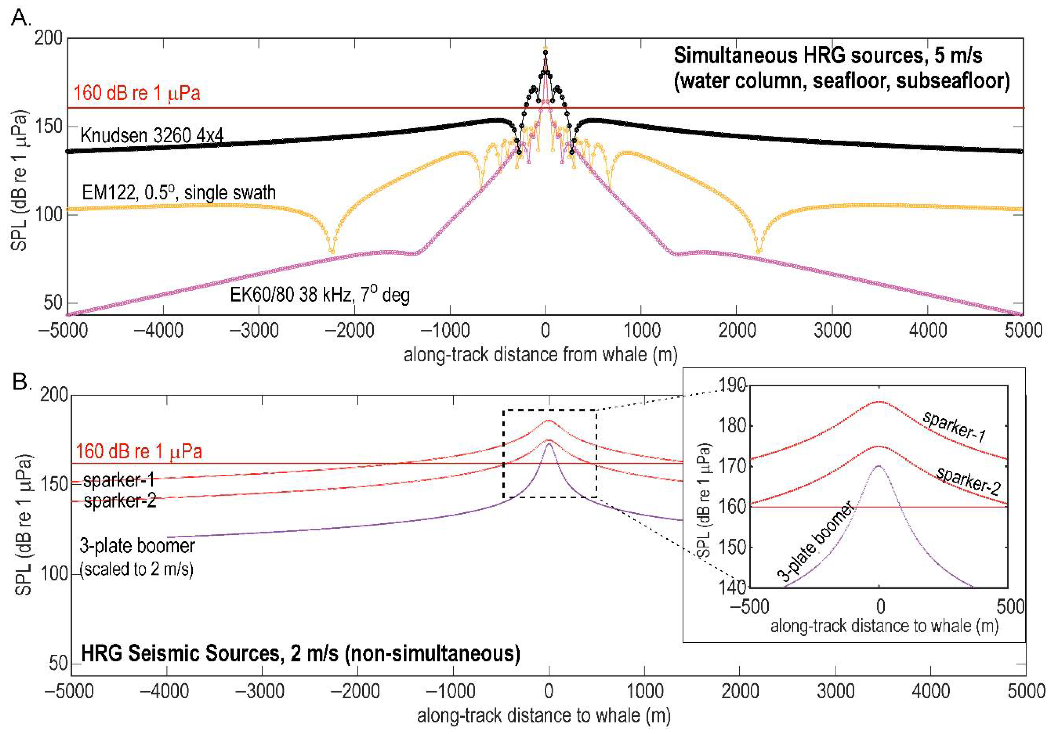
4.2. Multiple Acoustic Sources Used Simultaneously

Section 3 focused on the analysis of individual acoustic sources, but many marine surveys—whether conducted by commercial, research, or governmental entities—simultaneously deploy multiple acoustic sources. Simultaneous use of different acoustic sources saves resources and survey time and can ultimately reduce the impact on the environment and on marine animals if different data types can be acquired on a single survey pass. To elucidate the connections among dynamic ocean systems and processes, it is frequently necessary to acquire multiple data types during a single snapshot in time, which also requires the simultaneous use of multiple acoustic sources. In remote areas, simultaneous deployment of multiple acoustic sources leads to richer data sets being acquired during the rare surveys that can reach these locations.

A few examples illustrate the importance and pervasiveness of simultaneous deployment of acoustic sources. On research vessels, it has become routine to simultaneously acquire ADCP, SBES, MBES, and hull-mounted SBP data to facilitate characterization of the water column, seafloor, and subseafloor during a single pass. Much of the world’s seafloor remains unmapped [89], and routine, opportunistic use of MBES during transits or during surveys with other HRG sources could make substantial strides in addressing this knowledge gap for U.S. waters [90].

The challenge for use of multiple, simultaneous sources is how to assess the impact within the framework defined here. Under current practice, geophysical surveys that rise to the level of requiring an IHA for compliance with the MMPA provide documentation describing all acoustic sources to be used, with take calculations focused on the most impactful source. For example, for an airgun survey that simultaneously uses a MBES to map the seafloor, any Level A or B take estimations are based on the airguns, which produce the larger 160 dB zone. Ref. [91] adopted a different approach, calculating the ensonified area that exceeded the received SPL of 160 dB re 1 μPa for each larger acoustic source and the fraction of time that the sources were historically used alone or simultaneously during research cruises. This information, combined with animal densities, allowed for the calculation of estimated takes for all sources. This approach does not, however, account for the degree of exposure (Factor 5), which we have demonstrated could be used to render nearly all non-seismic HRG sources de minimis in their own right.

Figure 14A shows the SPL for simultaneous use of MBES, SBES (EK60/80), and Knudsen 3260 with synchronized pulses, as is common during surveys on large research vessels. Individually, each acoustic source has degree of exposure criteria within the schematic de minimis grouping in Figure 10, and the EK60/80 is also considered de minimis on the basis of beamwidth. Summing the maximum pings and exposure duration above 160 dB re 1 μPa for each instrument yields a maximum of 23 pings over 105 s for the animal at 100 m water depth in the unlikely scenario in which an animal remains stationary and is in precisely the correct position to receive all the pings. When only the MBES and SBES are operating, a stationary animal would only receive one ping above 160 dB re 1 μPa when the vessel is less than 50 m away in the x-direction. If the Knudsen 3260 were also operating, the ensonification cone would be ~57 m in diameter at 100 m depth, and most marine animals would require less than 30 s to move away from the ship’s track and the most direct effects of the instrument. We conclude that this single pass using all three instruments is unlikely to lead to incidental take, whereas three separate passes using each instrument, in turn, would re-ensonify the same part of the ocean, lead to increased vessel noise and risk of vessel strike, and statistically increase the possibility of a marine animal receiving high SPL signals. Therefore, the least impactful approach to this survey would be to use the three sources simultaneously in a single pass. We could also consider the effects on turtles. Although the transmission frequency of the sound sources described in this paragraph is largely outside the underwater frequency range for turtle hearing (which is up to ~1.6 kHz [61]), it is protective for turtles if a ship takes a single pass acquiring data with multiple acoustic sources instead of using the sources sequentially on multiple passes through the same area.

Based on these arguments, surveys that simultaneously deploy multiple, non-impulsive de minimis sources are unlikely to result in incidental take of marine mammals. We, therefore, suggest that HRG surveys that use one or more such sources at a time should be treated as wholly de minimis actions.

4.3. Behavioral Considerations

So far, we have analyzed the potential impact of marine acoustic sources based on the physical characteristics of the sources themselves, as well as the likelihood that an animal would encounter these sound sources. Although generally beyond the scope of this paper, the biological and behavioral context of marine animals should also be considered. Below, we briefly discuss behavioral evidence drawn from observations of marine mammals during the use of HRG sources to provide qualitative support for our determination that many HRG sources are unlikely to lead to incidental take and can therefore be deemed de minimis.

We first consider direct observations related to the impact of MBES systems on marine mammals during carefully formulated field studies. The hearing range of some cetaceans overlaps with the dominant frequencies emitted by some hull-mounted MBES systems (e.g., Figure 4B), and researchers, therefore, focus on the possibility of behavioral changes in response to exposure to MBES signals. Ref. [92] used a fixed, bottom-mounted hydrophone array in the USN’s Southern California Offshore Range (1800 km² area) to carefully identify vocalizations of Cuvier’s beaked whales during EM122 (12 kHz) MBES operations in 2017. The study also included periods when multiple hull-mounted acoustic sources (MBES, SBES, SBP) were operating together. The only marine mammal behavioral metric that changed among the periods before, during, and after exposure to the acoustic sources was the number of group vocalization periods per hour, with the vocalizations actually increasing during and after active MBES periods. Across the whole study, there was no difference in the number of clicks or the duration of vocalization events across the three periods. These results suggest that animals did not leave the area, nor did they cease foraging. Ref. [92] and an expanded study [93] conclude that the foraging effort did not change and that shifts in the location of the foraging for the 2019 survey could not be unequivocally linked to the acoustic survey.

Other studies have examined the response of whales to SBES, which are most often used to ensonify the water column for quantitative fisheries studies. Ref. [94] tagged nine short-finned pilot whales offshore Cape Hatteras and exposed five of them to an SBES (EK60). While these animals did not change their foraging behavior, they showed more variance in their directionality, suggesting increased vigilance while the SBES was active. However, because the nine individuals exhibited a range of behaviors, it was difficult to associate behavioral changes with active SBES transmission periods, and the authors acknowledged that the observed behavioral responses were subtle and not likely to be biologically significant. Ref. [95] also investigated the impact of SBES on toothed whales, conducting visual and acoustic surveys of beaked whales offshore southern New England during the use of EK60 transducers with frequencies overlapping the whales’ hearing range. A towed hydrophone array enabled these researchers to detect vocalization events but not the exact bearing of individual whales or group size. Although the results may not reach the level of statistical significance (p-value of 0.069), the study recorded fewer beaked whale vocalizations when the EK60 was actively transmitting, suggesting that animals either moved away from the area or reduced foraging activity. Ref. [96] examined the effects of a 38 kHz EK60 on Blainville’s beaked whales at the USN hydrophone-instrumented range near the Bahamas and found that click durations remain unchanged before, during, and after exposure to the sound source.

Taken together, these findings indicate that some species of toothed whales may show subtle behavioral responses when exposed to MBES or SBES, but factors such as behavioral context, location, and prey availability may be as important or even more important than the acoustic signals themselves. The behavioral evidence available in these studies suggests that MBES and SBES are unlikely to result in the incidental take of marine mammals, which is consistent with the physics-based de minimis determinations we made in Section 3.3.

4.4. Intermittency

As presently formulated, the degree of exposure criterion (Factor 5; Section 3.3.5) that renders many HRG sources de minimis has no dependence on pulse length (ping duration). Instead, the only pulse-related factor considered is exposure duration (pings plus intervening silence) to pings at SPL greater than 160 dB re 1 μPa. Using only the ping rate, without explicit consideration of pulse length, is consistent with NMFS’s alternative method of evaluating a moving, intermittent, non-impulsive source for Level A effects based on single pulse SEL in the user spreadsheet provided with [18].

Ref. [1] has recently recommended that the intermittency of a marine acoustic source be considered in evaluating behavioral responses. However, there has so far been little evidence to indicate that intermittent pulses lead to specific behaviors. Ref. [97] summarizes studies of marine mammal avoidance behavior in response to continuous and intermittent sounds that overlap different parts of the animals’ hearing range (Figure 4B), but no specific behaviors that could be interpreted as a function of intermittency were identified. Ref. [98] discusses the behavior of a captive mammal in response to intermittent military sonar signals, and [99] demonstrates a relationship between harbor porpoise sound detection thresholds for sounds of different duration and transmission frequency, with the animals less sensitive to short duration sounds and lower frequencies. This latter result focuses on hearing, not behavior, but presumably, an animal will not react to a sound until it is detected, meaning that behavior could also depend on the intermittency of a source. Intuitively, an animal could be expected to react differently to one hundred 50 ms pulses repeated at 2 s intervals (2.5% duty cycle) than to the same number of 1 s pulses at the same interval (50% duty cycle).

The NMFS user spreadsheet [18] calculation for the Level A “safe distance” from a moving, intermittent, non-impulsive acoustic source for different marine mammal hearing groups based on SPL_rms (called SPL in this paper) depends on pulse length through its inclusion of duty cycle. The NMFS calculation is based on [74], where safe distance ${\stackrel{⌢}{R}}_{0\_SEL}$ is given by:

$${\stackrel{⌢}{R}}_{0\_SEL}=\frac{\pi D_c}{v}{10}^{(SL-SE{L}_0)/(10 \mathrm{dB})}.$$

(5)

In (5), v is ship velocity, D_c denotes duty cycle of the source, and SEL₀ represents the threshold for response. Equation (5) is independent of transmission frequency, applies for an omnidirectional source with spherical spreading, and relies only on geometrical arguments about an animal’s position relative to the source. For Level A calculations, [18] uses the SEL_cum threshold for each marine mammal hearing group for SEL₀. Figure S9 explores an example of completing this calculation using a hypothetical SEL_cum of 190 dB, which is within the ranges of the marine mammal hearing groups used by [18]. We vary the duty cycle to schematically illustrate the impact of different pulse lengths on the determination of the safe distance. The results in Figure S9 do not convey information relevant to incidental take or to sources with directionality. However, they do underscore that, even without considering how an animal perceives sound (Section 4.5), pulse length should be a factor in assessing the impact of acoustic sources and eventually included in Factor 5 and taken into account in the assessment of Level B harassment thresholds.

4.5. Auditory Integration Time

All sensors, including animal auditory systems, integrate received sound levels over a finite time period. For assessing the effects of intermittent signals produced by many HRG sources, the critical observation is that signals much shorter than the animal’s integration time are perceived as having lower energy. In the current U.S. regulatory environment, hearing integration time is not explicitly considered when evaluating proposed actions under the MMPA or the ESA. Ref. [100] has recently underscored the importance of accounting for integration time, which depends on the frequency, intensity, and duration of sounds, in evaluating the behavioral effects of acoustic sources. Ref. [101] shows that considering a hearing integration time of 100 ms greatly reduces the distance to the 160 dB re 1 μPa Level B isopleth, even for omnidirectional, impulsive sources such as sparkers (e.g., 195 m vs. 33 m for the specific sparker and operational parameters described therein). Ref. [102] compiled the scant available data on marine mammal auditory integration time, noting the dependence on frequency (i.e., lower frequency leads to longer integration times). Some animal studies cited by [102] found integration times in the range of tens to hundreds of milliseconds, although narrowband clicks may be associated with integration times as short as hundreds of microseconds. As one example, consider the auditory integration time of 134 ms that [99] determined for harbor porpoises (HF cetaceans) in relation to some non-impulsive HRG sources discussed here. EM122 pulse length of 15 ms (for water depths < 2500 m) and a typical Knudsen 3260 pulse length of 16 ms represent less than 12% of the harbor porpoise’s auditory integration time. EM302 pulse lengths are typically 7 ms or shorter at water depths up to 3000 m, an even smaller fraction of the integration time. Boomer pulse length is less than 1 ms (less than 1% of the integration time). Thus, animals could perceive these sources as having lower energy than the modeled values shown in Figure 11, Figure 12, Figure 13 and Figure 14. A more sophisticated approach could be adopted using the computer programs provided by [100].

As more data are acquired about auditory integration times, the degree of exposure criteria described in Section 3.3.5 could be revised to explicitly incorporate consideration of pulse length on the source side and the integration time on the animal side. Based on preliminary information, the incorporation of appropriate auditory integration time is expected to show that the short pulse lengths of most non-impulsive HRG sources render them even less likely to lead to incidental take than our analysis has indicated.

5. Conclusions

To advance a framework for categorizing commonly deployed controlled acoustic sources based on their potential impact on marine animals, we develop criteria for assessing physical source characteristics (e.g., transmission frequency, source level, beamwidth, directionality, degree of exposure) and sort the sources into tiers (Table 3) that could inform regulatory evaluation under current U.S. environmental statutes. This framework can be easily adapted if behavioral thresholds were to change in the future. To broaden the utility of this study within the context of the ESA, we also briefly consider sea turtle densities (Figure S6a) for some of the criteria. We suggest periodic updating of the criteria used here for de minimis determinations in order to adapt to new information about certain sources (e.g., those in Tier 3), changing behavioral harassment thresholds, new data (e.g., on auditory integration time), or new approaches that could better account for all aspects of potential Level B harassment from acoustic sources (e.g., pulse length, directionality).

Based on this analysis, we divide the marine acoustic sources we consider here into four tiers. Tier 1 applies to high energy airgun or GI gun surveys and includes single airguns or airgun arrays of total volume greater than 1500 in³ and/or more than 12 airguns (or GI guns). Tier 2 covers the remaining low/intermediate energy airgun deployments that fall below the Tier 1 level. The true impact of an airgun survey is a function of a complex matrix of characteristics (i.e., number of guns, gun volumes, array tow depth, gun separation, water depth, seafloor reflectivity [32]), but the simple distinction that we propose between Tiers 1 and 2 is more straightforward to implement and emerges naturally from a consideration of peak source levels for actual surveys and for airguns measured during sound source verification experiments (Figure 3). Tiers 1 and 2 would likely lead to different levels of impact on the marine environment, and different degrees of mitigation and monitoring may therefore be appropriate.

Our analysis shows that most non-seismic HRG sources, as well as most oceanographic and communication/tracking acoustic sources, are unlikely to result in incidental take of marine mammals (Table 2). These de minimis sources constitute Tier 4 and may not warrant formal review under some environmental statutes. Examples of Tier 4 sources include MBES, hull-mounted and the shallow-towed SBPs tested by [8], sidescan sonars, three-plate boomers, split-beam fisheries sonars (also called SBES; e.g., EK60/80), low-powered sparkers, and acoustic releases, acoustic locators, and many systems used for underwater navigation and communication. Parametric SBPs are included in the Tier 4 de minimis category based not on our analysis, but on the previous precedent established by NMFS (e.g., 85 FR 26941 [78]). Some USBLs have also previously been considered unlikely to lead to incidental take in NMFS analyses (e.g., 85 FR 30933 [79]).

Non-airgun HRG seismic sources are mostly placed within Tier 3, as their level of impact falls between that of low-energy airguns (Tier 2) and de minimis sources (Tier 4). Sparkers other than those operated at the lowest SL do not automatically meet the de minimis criteria. As more data are acquired (e.g., [81]), certain combinations of water depth and sparker SL, along with the implementation of certain mitigation and monitoring measures, could render such sparker surveys functionally equivalent to a de minimis action. In the case of bubble guns and one- and two-plate boomers, some or even most surveys could eventually meet de minimis criteria or be rendered functionally equivalent to de minimis with operational restrictions and/or monitoring and mitigation mandates. At present, insufficient information about their directionality and other characteristics leads us to categorize them as Tier 3. We provide no tiering for marine vibrators, which are still in the experimental stage.

We also do not analyze the complete class of underwater navigation systems (i.e., LBL, SBL, and USBL). These systems tend to be stationary during operations, may have SL greater than 200 dB re μPa @ 1 m, frequencies less than 180 kHz, and omnidirectional or large-beamwidth transmissions, and should be further examined to determine their effects on marine animals. However, if such systems are deemed critical for the safety of divers or vehicles, they would be placed in the same class as ships’ fathometers and not further scrutinized.

To evaluate new technologies or controlled marine acoustic sources not considered here, we suggest first identifying the source that we analyzed whose characteristics (e.g., SL or SPL, transmission frequency, beamwidth, degree of exposure) are closest to the unassessed source and then determining whether the existing analysis could be applied to the unassessed source. If not, then the unassessed source should be independently evaluated using the factors outlined in Section 3.3, with any determination about tiering of the source fully documented. Note that the framework defined was applied using the current Level B criteria applied under the MMPA and ESA, but changes to the Level B thresholds are easily incorporated by modifying Factors 2 through 5 accordingly.

Simultaneous use of multiple acoustic sources is common practice in marine operations to map, characterize, and explore ocean environments. We suggest that the use of multiple, non-impulsive de minimis sources could render the entire operation de minimis when considering acoustic effects. When de minimis sources (e.g., MBES) are used along with sources in Tiers 1 through 3, the regulatory review standard that applies to the most impactful tier could be applied to the entire marine survey, in agreement with current practice. However, the independent deployment of de minimis sources while the Tier 1 through Tier 3 source is not in use during the same survey is by definition unlikely to lead to incidental take and should not be treated differently than any other use of a de minimis source.

The widespread adoption of uniform tiers for marine acoustic sources by all constituencies involved in marine exploration, mapping, and characterization activities could lead to more consistent and more efficient environmental compliance. Regulatory resources would be more efficiently expended by focusing on the most impactful acoustic sources, which are categorized here in Tiers 1 through 3. Tier 4 (de minimis) sources, which represent many of the non-seismic sources routinely deployed in U.S. waters for civilian activities, are unlikely to result in incidental take of marine mammals; therefore survey-by-survey regulatory review should be unnecessary for single or multiple Tier 4 sources. Indeed, the MMC has repeatedly emphasized that HRG sources, like some of those that we place in de minimis Tier 4, should not need reviews under the MMPA, while impulsive HRG seismic sources (e.g., sparkers, Tier 3) should be more formally evaluated. For some Tier 3 sources, it could be possible to formulate an operational matrix (e.g., source levels, water depths) and a suite of monitoring and mitigation measures that effectively render the source de minimis in practical terms for most surveys.

References

1. Southall, B.L.; Nowacek, D.P.; Bowles, A.E.; Senigaglia, V.; Bejder, L.; Tyack, P.L. Marine Mammal Noise Exposure Criteria: Assessing the Severity of Marine Mammal Behavioral Responses to Human Noise. Aquat. Mamm. 2021, 47, 421–464. [Google Scholar] [CrossRef]
2. Clay, C.S.; Medwin, H. Acoustical Oceanography: Principles and Applications; Wiley: Taipei, Taiwan, 1979; p. 576. [Google Scholar]
3. Kinsler, L.E.; Frey, A.R.; Coppens, A.B.; Sanders, J.V. Fundamentals of Acoustics, 4th ed.; Wiley-VCH: Hoboken, NJ, USA, 1999; p. 560. [Google Scholar]
4. Pierce, A.D. Acoustics: An Introduction to Its Physical Principles and Applications, 3rd ed.; Springer International: Cham, Switzerland, 2019; p. 768. [Google Scholar]
5. Urick, R.J. Principles of Underwater Sound; Peninsula Publishing: Los Altos, CA, USA, 1983; p. 444. [Google Scholar]
6. Lurton, X. An Introduction to Underwater Acoustics: Principles and Applications; Springer: London, UK, 2002; p. 777. [Google Scholar]
7. International Organization for Standardization (ISO). ISO 18405:2017 Underwater Acoustics—Terminology; ISO: Geneva Switzerland, 2017; Available online: https://www.iso.org/standard/62406.html (accessed on 11 June 2020).
8. Crocker, S.E.; Fratantonio, F.D. Characteristics of Sounds Emitted During High-Resolution Geophysical Surveys; NUWC-NPT Technical Report 12203; Naval Undersea Warfare Center Division-Newport: Newport, RI, USA, 2016; p. 266. Available online: https://apps.dtic.mil/sti/pdfs/AD1007504.pdf (accessed on 27 September 2020).
9. Applied Acoustics Engineering Ltd. High Power Sparker Systems. 2013. Available online: https://www.subseatechnologies.com/media/files/files/b38eaa45/delta-sparker-brochure.pdf (accessed on 21 July 2021).
10. Feltham, A.; Girard, M.; Jenkerson, M.; Nechayuk, V.; Griswold, S.; Henderson, N.; Johnson, G. The Marine Vibrator Joint Industry Project: Four years on. Explor. Geophys. 2018, 49, 675–687. [Google Scholar] [CrossRef]
11. National Marine Fisheries Service (NMFS). Takes of Marine Mammals Incidental to Specified Activities; Taking Marine Mammals Incidental to Site Characterization Surveys of Lease Areas. Fed. Regist. 2019, 84, 52464–52488. Available online: https://www.federalregister.gov/documents/2019/10/02/2019-21458/takes-of-marine-mammals-incidental-to-specified-activities-taking-marine-mammals-incidental-to-site (accessed on 23 February 2021).
12. GEO Marine Survey Systems. Mega-Spark 20–40 kJ. 2020. Available online: https://www.geomarinesurveysystems.com/downloads/brochures/Geo-Spark_20-40kJ.pdf (accessed on 22 February 2021).
13. National Marine Fisheries Service (NMFS). Takes of Marine Mammals Incidental to Specified Activities; Taking Marine Mammals Incidental to Marine Site Characterization Surveys Off of Delaware and Maryland. Fed. Regist. 2019, 84, 66156–66175. Available online: https://www.federalregister.gov/documents/2019/12/03/2019-26091/takes-of-marine-mammals-incidental-to-specified-activities-taking-marine-mammals-incidental-to (accessed on 23 February 2021).
14. Kongsberg. TOPAS PS18. 2019. Available online: https://www.kongsberg.com/globalassets/maritime/km-products/product-documents/topas-ps-18-parametric-sub-bottom-profiler.pdf (accessed on 10 February 2021).
15. Innomar. Products. Available online: https://www.innomar.com/products.php (accessed on 10 February 2021).
16. National Ocean Service. Final Programmatic Environmental Assessment for the Office of Coast Survey Hydrographic Survey Projects; National Oceanic and Atmospheric Administration: Silver Spring, MD, USA, 2013; p. 128. Available online: https://nauticalcharts.noaa.gov/about/docs/regulations-and-policies/2013-18-nepa-ocs-final-pea.pdf (accessed on 24 February 2021).
17. Southall, B.L.; Bowles, A.; Ellison, W.; Finneran, J.J.; Gentry, R.L.; Green, C.R.; Kastak, C.R.; Ketten, D.; Miller, J.; Nachtigall, P.; et al. Marine mammal noise exposure criteria. Aquat. Mamm. 2007, 33, 411–414. [Google Scholar] [CrossRef]
18. National Marine Fisheries Service (NMFS). 2018 Revision to: Technical Guidance for Assessing the Effects of Anthropogenic Sound on Marine Mammal Hearing (Version 2.0): Underwater Thresholds for Onset of Permanent and Temporary Threshold Shifts, NOAA Technical Memorandum, NMFS-OPR-59; National Oceanic and Atmospheric Administration (NOAA): Washington, DC, USA, 2018; p. 167. Available online: https://media.fisheries.noaa.gov/dam-migration/tech_memo_acoustic_guidance_%2820%29_%28pdf%29_508.pdf (accessed on 21 December 2019).
19. National Marine Fisheries Service (NMFS). Endangered Fish and Wildlife; Notice of Intent to Prepare an Environmental Impact Statement. Fed. Regist. 2005, 70, 1871–1875. Available online: https://www.federalregister.gov/documents/2005/01/11/05-525/endangered-fish-and-wildlife-notice-of-intent-to-prepare-an-environmental-impact-statement (accessed on 24 June 2022).
20. National Marine Fisheries Service (NMFS). Takes of Marine Mammals Incidental to Specified Activities; Low-Energy Marine Geophysical Survey in the Dumont d’Urville Sea Off the Coast of East Antarctica, January to March 2013. Fed. Regist. 2014, 79, 463–497. Available online: https://www.federalregister.gov/documents/2014/01/03/2013-31471/takes-of-marine-mammals-incidental-to-specified-activities-low-energy-marine-geophysical-survey-in (accessed on 24 June 2022).
21. Tyack, P.L.; Zimmer, W.M.X.; Moretti, D.; Southall, B.L.; Claridge, D.E.; Durban, J.W.; Clark, C.W.; D’Amico, A.; DiMarzio, N.; Jarvis, S.; et al. Beaked Whales Respond to Simulated and Actual Navy Sonar. PLoS ONE 2011, 6, e17009. [Google Scholar] [CrossRef]
22. RD Instruments. ADCP Beam Clearance Area, Teledyne Application Note FSA-019; Teledyne RDI: San Diego, CA, USA, 2002; p. 8. Available online: http://www.teledynemarine.com/Documents/Brand%20Support/RD%20INSTRUMENTS/Technical%20Resources/Technical%20Notes/ChannelMaster/FSA019.PDF (accessed on 15 October 2020).
23. Simrad. EK80 Wide Band Scientific Echo Sounder: Installation Manual, 394149/D. 2020. Available online: https://www.simrad.online/ek80/ins/ek80_ins_en_us.pdf (accessed on 3 September 2021).
24. Richardson, W.J.; Greene, C.R.; Malme, C.I.; Thomson, D.H. Chapter 6—Man Made Noise. In Marine Mammals and Noise; Richardson, W.J., Greene, C.R., Malme, C.I., Thomson, D.H., Eds.; Academic Press: San Diego, CA, USA, 1995; pp. 101–158. [Google Scholar]
25. National Science Foundation (NSF); U.S. Geological Survey (USGS). Final Programmatic Environmental Impact Statement/Overseas Environmental Impact statement for Marine Seismic Research funded by the National Science Foundation or conducted by the U.S. Geological Survey; National Science Foundation (NSF): U.S. Geological Survey (USGS): Arlington, VA, USA; Reston, VA, USA, 2011; p. 981. Available online: https://www.nsf.gov/geo/oce/envcomp/usgs-nsf-marine-seismic-research/nsf-usgs-final-eis-oeis_3june2011.pdf (accessed on 3 April 2013).
26. International Association of Geophysical Contractors (IAGC). Lowest Practicable Source Levels (LPSL): The Implications of Adjusting Seismic Source Array Parameters. 2014. Available online: https://iagc.org/wp-content/uploads/2020/07/IAGC-Working-Paper-Lowest-Practicable-Source-Level-Dec-2014.pdf (accessed on 10 November 2014).
27. Farmer, P.; Miller, D.; Pieprzak, A.; Rutledge, J.; Woods, R. Exploring the Subsalt. Oilfield Rev. 1996, 8, 50–64. [Google Scholar]
28. Holbrook, W.S.; Reiter, E.C.; Purdy, G.M.; Toksöz, M.N. Image of the Moho across the continent-ocean transition, U.S. east coast. Geology 1992, 20, 203–206. [Google Scholar] [CrossRef]
29. Kent, G.M.; Singh, S.C.; Harding, A.J.; Sinha, M.C.; Orcutt, J.A.; Barton, P.J.; White, R.S.; Bazin, S.; Hobbs, R.W.; Tong, C.H.; et al. Evidence from three-dimensional seismic reflectivity images for enhanced melt supply beneath mid-ocean ridge discontinuities. Nature 2000, 406, 614–618. [Google Scholar] [CrossRef] [PubMed]
30. Keen, C.E.; de Voogd, B. The continent-ocean boundary at the rifted margin off eastern Canada: New results from deep seismic reflection studies. Tectonics 1988, 7, 107–124. [Google Scholar] [CrossRef]
31. Dragoset, W.H. Air-gun array specs: A tutorial. Lead. Edge 1990, 9, 24–32. [Google Scholar] [CrossRef]
32. Caldwell, J.; Dragoset, W. A brief overview of seismic air-gun arrays. Geophysics 2000, 19, 898–902. [Google Scholar] [CrossRef]
33. Lawrence, M.; Oxley, I.; Bates, C. Geophysical Techniques for Maritime Archaeological Surveys. In Proceedings of the Symposium on the Application of Geophysics to Engineering and Environmental Problems 2004, Colorado Springs, CO, USA, 22–26 February 2004. [Google Scholar] [CrossRef] [Green Version]
34. Hill, P.R.; Barrie, J.V.; Kung, R.; Lintern, D.G.; Mullan, S.; Li, M.Z.; Shaw, J.; Stacey, C.D.; Todd, B.J. Geological and Geophysical Site Characterization for Marine Renewable Energy Development and Environmental Assessment; Technical Report No. EXPO3-2015; CSA Group: Toronto, ON, Canada, 2015; p. 131. [Google Scholar] [CrossRef]
35. Foley, J.; Jennings, D.; Fonda, R.; Jacobson, J.; Miele, M. Improved capability, reliability, and productivity for underwater geophysical mapping of unexploded ordnance. In Proceedings of the OCEANS 2015—Genova, Genova, Italy, 18–21 May 2015; pp. 1–6. [Google Scholar] [CrossRef]
36. Williams, S.J.; Cichon, H.A. Geologic Assessments and Characterization of Marine sand Resources—Gulf of Mexico Region. In Proceedings of the 8th Symposium on Coastal and Ocean Management, New Orleans, LA, USA, 19–23 July 1993; Available online: http://pubs.er.usgs.gov/publication/70017792 (accessed on 21 October 2021).
37. Guan, S.; Brookens, T.; Vignola, J. Use of Underwater Acoustics in Marine Conservation and Policy: Previous Advances, Current Status, and Future Needs. J. Mar. Sci. Eng. 2021, 9, 173. [Google Scholar] [CrossRef]
38. Applied Acoustics Engineering Ltd. S-Boom System. 2020. Available online: https://www.aaetechnologiesgroup.com/wp-content/uploads/2021/02/S-Boom-%E2%80%93-Technical-Specification.pdf (accessed on 12 February 2021).
39. Falmouth Scientific. HMS-620 Bubble Gun. 2019. Available online: https://www.falmouth.com/files/HMS-620BubbleGun.pdf (accessed on 11 February 2021).
40. Falmouth Scientific. HMS-620LF Bubble Gun. 2020. Available online: https://www.falmouth.com/files/HMS-620LFLowFrequencyBubbleGun.pdf (accessed on 7 September 2022).
41. Wunderlich, J.; Müller, S. High-resolution sub-bottom profiling using parametric acoustics. Int. Ocean. Syst. 2003, 7, 6–11. [Google Scholar]
42. Demer, D.A.; Andersen, L.N.; Bassett, C.; Berger, L.; Chu, D.; Condiotty, J.; Cutter, G.R. 2016 USA–Norway EK80 Workshop Report: Evaluation of a Wideband Echosounder for Fisheries and Marine Ecosystem Science; ICES Cooperative Research Report No. 336; International Council for the Exploration of the Sea: Copenhagen, Denmark, 2017; p. 79. Available online: https://www.ices.dk/sites/pub/Publication%20Reports/Cooperative%20Research%20Report%20(CRR)/CRR336.pdf (accessed on 14 October 2020).
43. Edgetech. Coastal Acoustic Transponder. Available online: https://www.edgetech.com/wp-content/uploads/2019/07/ETN-ET-5491-CAT-3_31_22-073013-1.pdf (accessed on 21 August 2022).
44. Teledyne Marine. Teledyne Benthos Location and Recovery. Available online: http://www.teledynemarine.com/Lists/Downloads/Locator_Brochure_2015_lo.pdf (accessed on 21 August 2022).
45. Applied Acoustics Engineering Ltd. Easytrak M-USBL, Model 2671. Available online: https://www.aaetechnologiesgroup.com/wp-content/uploads/2021/02/Easytrak-M-USBL-2671-%E2%80%93-Technical-Specification.pdf (accessed on 21 August 2022).
46. Edgetech. Multibeacon, Model 4380 Transponder/Responder. Available online: https://www.edgetech.com/wp-content/uploads/2019/07/4830-Multibeacon091014.pdf (accessed on 21 August 2022).
47. Sonardyne. Datasheet, HPT 50000/7000, Ultra-short baseline and telemetry receiver. Available online: https://www.sonardyne.com/wp-content/uploads/2021/06/Sonardyne_8142_HPT.pdf (accessed on 21 August 2022).
48. Ellison, W.T.; Southall, B.L.; Clark, C.W.; Frankel, A.S. A New Context-Based Approach to Assess Marine Mammal Behavioral Responses to Anthropogenic Sounds. Conserv. Biol. 2012, 26, 21–28. [Google Scholar] [CrossRef]
49. Gomez, C.; Lawson, J.W.; Wright, A.J.; Buren, A.D.; Tollit, D.; Lesage, V. A systematic review on the behavioural responses of wild marine mammals to noise: The disparity between science and policy. Can. J. Zool. 2016, 94, 801–819. [Google Scholar] [CrossRef]
50. U.S. Navy (USN). Chapter 3 Affected Environment and Environmental Consequences. In Final Environmental Impact Statement/Overseas Environmental Impact Statement Atlantic Fleet Training and Testing; United States Department of the Navy: Washington, DC, USA, 2018; pp. 1–144. Available online: https://media.defense.gov/2020/May/13/2002299473/-1/-1/1/3.00%20AFTT%20FEIS%20AFFECTED%20EVIRIRONMENT%20AND%20ENVIRONMENTAL%20CONSEQUENCES.PDF (accessed on 9 October 2020).
51. National Marine Fisheries Service (NMFS). Takes of Marine Mammals Incidental to Specified Activities; Taking Marine Mammals Incidental to Office of Naval Research Arctic Research Activities. Fed. Regist. 2019, 84, 37240–37262. Available online: https://www.federalregister.gov/documents/2019/07/31/2019-16318/takes-of-marine-mammals-incidental-to-specified-activities-taking-marine-mammals-incidental-to (accessed on 8 September 2021).
52. Gisiner, R.C. Sound and marine seismic surveys. Acoust. Today 2016, 12, 10–18. [Google Scholar]
53. Crocker, S.E.; Fratantonio, F.D.; Hart, P.E.; Foster, D.S.; O’Brien, T.F.; Labak, S. Measurement of Sounds Emitted by Certain High-Resolution Geophysical Survey Systems. IEEE J. Ocean. Eng. 2019, 44, 796–813. [Google Scholar] [CrossRef]
54. National Marine Fisheries Service (NMFS). Takes of Marine Mammals Incidental to Specified Activities; Taking Marine Mammals Incidental to Marine Site Characterization Surveys Off of Massachusetts and Rhode Island. Fed. Regist. 2021, 86, 40469–40494. Available online: https://www.federalregister.gov/documents/2021/07/28/2021-16025/takes-of-marine-mammals-incidental-to-specified-activities-taking-marine-mammals-incidental-to (accessed on 14 September 2021).
55. U.S. Fish and Wildlife Service (USFWS). Marine Mammals; Incidental Take during Specified Activities: Cook Inlet, Alaska. Fed. Regist. 2019, 84, 2–36. Available online: https://www.federalregister.gov/documents/2019/08/01/2019-16279/marine-mammals-incidental-take-during-specified-activities-cook-inlet-alaska (accessed on 14 September 2021).
56. Marine Mammal Commission (MMC). Comment letter on: Equinor Wind application under Section 105(a)(5)(D) of the Marine Mammal Protection Act. 2020. Available online: https://www.mmc.gov/wp-content/uploads/20-07-13-Harrison-NMFS-Equinor-proposed-IHA-HRG-surveys-NJ-NY-CT-RI-MA.pdf (accessed on 31 March 2021).
57. Kongsberg. EM122 Multibeam Echo Sounder: Product Description, Report 302440/E. 2011. Available online: https://epic.awi.de/id/eprint/45364/1/Kongsberg_302440ae_em122_product_description.pdf (accessed on 29 September 2020).
58. Hammerstad, E. EM Technical Note: Sound Levels from Kongsberg Multibeams. 2005, p. 3. Available online: https://www.kongsberg.com/globalassets/maritime/km-products/product-documents/em_technical_note_web_soundlevelsfromkongsbergmultibeams.pdf (accessed on 14 June 2020).
59. Teledyne Marine. Source Level of Teledyne RD Instruments ADCP Transducers, 2020. p. 3. Available online: http://www.teledynemarine.com/Documents/Brand%20Support/RD%20INSTRUMENTS/Technical%20Resources/Technical%20Notes/Technical%20Notes/FST054.PDF (accessed on 30 December 2020).
60. Popper, A.; Hawkins, A.; Fay, R.; Mann, D.; Bartol, S.; Carlson, T.; Coombs, S.; Ellison, W.; Gentry, R.; Halvorsen, M.; et al. Sound Exposure Guidelines. In Springer Briefs in Oceanography; Springer International: Cham, Switzerland, 2014; pp. 33–51. [Google Scholar]
61. Piniak, W.E.D.; Mann, D.A.; Harms, C.A.; Jones, T.T.; Eckert, S.A. Hearing in the Juvenile Green Sea Turtle (Chelonia mydas): A Comparison of Underwater and Aerial Hearing Using Auditory Evoked Potentials. PLoS ONE 2016, 11, e0159711. [Google Scholar] [CrossRef]
62. Smith, M.J. Analysis of the Radiated Sound Field of a Deep-Water Multibeam Echosounder Using a NAVY Hydrophone Array. Master’s Thesis, University of New Hampshire, Durham, NH, USA, 2019. [Google Scholar]
63. Deng, Z.D.; Southall, B.L.; Carlson, T.J.; Xu, J.; Martinez, J.J.; Weiland, M.A.; Ingraham, J.M. 200 kHz Commercial Sonar Systems Generate Lower Frequency Side Lobes Audible to Some Marine Mammals. PLoS ONE 2014, 9, e95315. [Google Scholar] [CrossRef]
64. National Marine Fisheries Service (NMFS). Takes of Marine Mammals Incident to Specified Activities; Taking Marine Mammals Incidental to Offshore Wind Construction Activities off of Virginia. Fed. Regist. 2020, 85, 14901–14924. Available online: https://www.federalregister.gov/documents/2020/03/16/2020-05281/takes-of-marine-mammals-incidental-to-specified-activities-taking-marine-mammals-incidental-to (accessed on 8 September 2021).
65. Roberts, J.J.; Best, B.D.; Mannocci, L.; Fujioka, E.; Halpin, P.N.; Palka, D.L.; Garrison, L.P.; Mullin, K.D.; Cole, T.V.N.; Khan, C.B.; et al. Habitat-based cetacean density models for the U.S. Atlantic and Gulf of Mexico. Sci. Rep. 2016, 6, 22615. [Google Scholar] [CrossRef]
66. Geo-Marine, I. Navy OpArea Density Estimates (NODE) for the Northeast OpAreas: Boston, Narrangansett Bay, and Atlantic City; Geo-Marine, Inc.: Plano, TX, USA, 2007; p. 217. Available online: https://seamap.env.duke.edu/downloads/resources/serdp/Northeast%20NODE%20Final%20Report.pdf (accessed on 14 March 2018).
67. Geo-Marine, I. Navy OpArea Density Estimates (NODE) for the Southeast OpAreas: VACAPES, CHPT, JAX/CHASN, and Southeastern Florida & AUTEC-Andros; Geo-Marine, Inc.: Plano, TX, USA, 2007; p. 197. Available online: https://seamap.env.duke.edu/downloads/resources/serdp/Southeast%20NODE%20Final%20Report.pdf (accessed on 14 March 2018).
68. Becker, E.A.; Forney, K.A.; Miller, D.L.; Fiedler, P.C.; Barlow, J.; Moore, J.E. Habitat-Based Density Estimates for Cetaceans in the California Current Ecosystem Based on 1991–2018 Survey Data; U.S. Department of Commerce, NOAA: Washington, DC, USA, 2020; p. 78. Available online: https://swfsc-publications.fisheries.noaa.gov/publications/CR/2020/2020Becker1.pdf (accessed on 12 April 2022).
69. NOAA National Geophysical Data Center. ETOPO1 1 Arc-Minute Global Relief Model. NOAA National Centers for Environmental Information. 2009. Available online: https://www.ncei.noaa.gov/access/metadata/landing-page/bin/iso?id=gov.noaa.ngdc.mgg.dem:316 (accessed on 17 June 2021).
70. Kremser, U.; Klemm, P.; Kotz, W.-D. Estimating the risk of temporary acoustic threshold shift, caused by hydroacoustic devices, in whales in the Southern Ocean. Antarct. Sci. 2005, 17, 3–10. [Google Scholar] [CrossRef]
71. Geo-Marine, I. Navy OpArea Density Estimates (NODE) for the GOMEX OPAREA; Geo-Marine, Inc.: Plano, TX, USA, 2007; p. 163. Available online: https://seamap.env.duke.edu/downloads/resources/serdp/Gulf%20of%20Mexico%20NODE%20Final%20Report.pdf (accessed on 3 September 2021).
72. National Marine Fisheries Service (NMFS). Taking and Importing Marine Mammals: Taking Marine Mammals Incidental to U.S. Navy Operations of Surveillance Towed Array Sensor System Low Frequency Active Sonar. Fed. Regist. 2017, 82, 19460–19527. Available online: https://www.federalregister.gov/documents/2017/04/27/2017-08066/taking-and-importing-marine-mammals-taking-marine-mammals-incidental-to-us-navy-operations-of (accessed on 14 September 2021).
73. National Marine Fisheries Service (NMFS). Takes of Marine Mammals Incidental to Specified Activities; Taking Marine Mammals Incidental to U.S. Navy Training and Testing Activities in the Northwest Training and Testing (NWTT) Study Area. Fed. Regist. 2020, 85, 72312–72469. Available online: https://www.federalregister.gov/documents/2020/11/12/2020-23757/taking-and-importing-marine-mammals-taking-marine-mammals-incidental-to-the-us-navy-training-and (accessed on 14 September 2021).
74. Sivle, L.D.; Kvadsheim, P.H.; Ainslie, M.A. Potential for population-level disturbance by active sonar in herring. ICES J. Mar. Sci. 2015, 72, 558–567. [Google Scholar] [CrossRef]
75. Lurton, X. Modelling of the sound field radiated by multibeam echosounders for acoustical impact assessment. Appl. Acoust. 2016, 101, 201–221. [Google Scholar] [CrossRef]
76. Willoughby, G.; MacDonald, N.; Darling, A.; Hiller, T. Applying Novel Sub-Bottom Boomer Technology to the Submerged Wellington Fault, New Zealand. In Proceedings of the Shallow Survey Conference, Wellington, New Zealand, 20–24 February 2012; p. 10. [Google Scholar]
77. National Marine Fisheries Service (NMFS). Taking and Importing Marine Mammals; Taking Marine Mammals Incidental to the U.S. Navy Training and Testing Activities in the Northwest Training and Testing (NWTT) Study Area. Fed. Regist. 2021, 86, 8490–8536. Available online: https://www.federalregister.gov/documents/2021/02/05/2021-02263/takes-of-marine-mammals-incidental-to-specified-activities-taking-marine-mammals-incidental-to (accessed on 6 May 2021).
78. National Marine Fisheries Service (NMFS). Takes of Marine Mammals Incidental to Specified Activities; Taking Mammals Incidental to Marine Site Characterization Surveys Off of Massachusetts, Rhode Island, Connecticut, and New York. Fed. Regist. 2020, 85, 26940–26962. Available online: https://www.federalregister.gov/documents/2020/05/06/2020-09629/takes-of-marine-mammals-incidental-to-specified-activities-taking-marine-mammals-incidental-to (accessed on 6 May 2021).
79. National Marine Fisheries Service (NMFS). Takes of Marine Mammals Incident to Specified Activities; Taking Marine Mammals Incidental to Offshore Wind Construction Activities off of Virginia. Fed. Regist. 2020, 85, 30933–30948. Available online: https://www.federalregister.gov/documents/2020/05/21/2020-10982/takes-of-marine-mammals-incidental-to-specified-activities-taking-marine-mammals-incidental-to (accessed on 8 September 2021).
80. U.S. Geological Survey (USGS). Determination of NEPA Adequacy: Low-Energy Geophysical Survey of the Queen Charlotte Fault, Southeastern Alaska; U.S. Geological Survey: Reston, VA, USA, 2017; p. 11. Available online: https://www.usgs.gov/media/files/determination-nepa-adequacy (accessed on 7 September 2022).
81. Balster-Gee, A.F.; Baldwin, W.E.; Hart, P.E. U.S. Geological Survey data release. Calibrated marine sparker source amplitude decay versus offset offshore Santa Cruz, California. 2022. Available online: https://www.usgs.gov/products/data/data-releases (accessed on 8 September 2022).
82. Teyssandier, B.; Sallas, J.J. The shape of things to come—Development and testing of a new marine vibrator source. Lead. Edge 2019, 38, 680–690. [Google Scholar] [CrossRef]
83. Laws, R.M.; Halliday, D.; Hopperstad, J.F.; Gerez, D.; Supawala, M.; Özbek, A.; Murray, T.; Kragh, E. Marine vibrators: The new phase of seismic exploration. Geophys. Prospect. 2019, 67, 1443–1471. [Google Scholar] [CrossRef]
84. Matthews, M.-N.R.; Ireland, D.S.; Zeddies, D.G.; Brune, R.H.; Pyć, C.D. A Modeling Comparison of the Potential Effects on Marine Mammals from Sounds Produced by Marine Vibroseis and Air Gun Seismic Sources. J. Mar. Sci. Eng. 2021, 9, 12. [Google Scholar] [CrossRef]
85. U.S. Geological Survey (USGS). Final Environmental Assessment of a Marine Geophysical Survey (MATRIX) by the US Geological Survey in the Northwestern Atlantic Ocean, August 2018; U.S. Geological Survey (USGS): Reston, VA, USA, 2018; p. 314. Available online: https://www.usgs.gov/media/files/final-environmental-assessment-a-marine-geophysical-survey-matrix (accessed on 7 September 2022).
86. LGL Ltd. Final Environmental Assessment of a Low-Energy Marine Geophysical Survey by the R/V Roger Revelle in the Northeastern Pacific Ocean, September 2017; LGL Ltd.: King City, ON, Canada, 2017; p. 404. Available online: https://www.nsf.gov/geo/oce/envcomp/scripps-oregon-final-ea.pdf (accessed on 22 February 2021).
87. National Marine Fisheries Service (NMFS). Takes of Marine Mammals Incidental to Specified Activities; Taking Marine Mammals Incidental to a Low-Energy Geophysical Survey in the Northeastern Pacific Ocean. Fed. Regist. 2017, 82, 29307–39276. Available online: https://www.federalregister.gov/documents/2017/08/17/2017-17378/takes-of-marine-mammals-incidental-to-specified-activities-taking-marine-mammals-incidental-to-a (accessed on 15 September 2021).
88. National Marine Fisheries Service (NMFS). Takes of Marine Mammals Incidental to Specified Activities; Taking Marine Mammals Incidental to a Marine Geophysical Survey in the Northwest Atlantic Ocean. Fed. Regist. 2018, 83, 39692–39709. Available online: https://www.federalregister.gov/documents/2018/08/10/2018-17170/takes-of-marine-mammals-incidental-to-specified-activities-taking-marine-mammals-incidental-to-a (accessed on 15 September 2021).
89. Wölfl, A.-C.; Snaith, H.; Amirebrahimi, S.; Devey, C.W.; Dorschel, B.; Ferrini, V.; Huvenne, V.A.I.; Jakobsson, M.; Jencks, J.; Johnston, G.; et al. Seafloor Mapping—The Challenge of a Truly Global Ocean Bathymetry. Front. Mar. Sci. 2019, 6, 283. [Google Scholar] [CrossRef]
90. Ocean Science and Technology Subcommittee. National Strategy for Mapping, Exploring, and Characterizing the United States Exclusive Economic Zone; Office of Science and Technology Policy: Washington, DC, USA, 2020; p. 25. Available online: https://iocm.noaa.gov/about/documents/strategic-plans/20200611-FINAL-STRATEGY-NOMEC-Sec.-2.pdf (accessed on 23 February 2021).
91. Southwest Fisheries Science Center (SWFSC). Request for Rulemaking and Letters of Authorization under Section 101(a)(5)(A) of the Marine Mammal Protection Act for the Take of Marine Mammals Incidental to Fisheries and Ecosystems Research Activities Conducted by NOAA Fisheries Southwest Fisheries Science Center within the California Current Ecosystem, Eastern Tropical Pacific Ecosystem, and Antarctic Ecosystem; NOAA Fisheries Southwest Fisheries Science Center: La Jolla, CA, USA, 2013; p. 210. Available online: https://media.fisheries.noaa.gov/dam-migration/swfsc_loa2015_application.pdf (accessed on 14 October 2020).
92. Kates Varghese, H.; Miksis-Olds, J.; DiMarzio, N.; Lowell, K.; Linder, E.; Mayer, L.; Moretti, D. The effect of two 12 kHz multibeam mapping surveys on the foraging behavior of Cuvier’s beaked whales off of southern California. J. Acoust. Soc. Am. 2020, 147, 3849–3858. [Google Scholar] [CrossRef] [PubMed]
93. Kates Varghese, H.; Lowell, K.; Miksis-Olds, J.; DiMarzio, N.; Moretti, D.; Mayer, L. Spatial Analysis of Beaked Whale Foraging During Two 12 kHz Multibeam Echosounder Surveys. Front. Mar. Sci. 2021, 8, 1139. [Google Scholar] [CrossRef]
94. Quick, N.; Scott-Hayward, L.; Sadykova, D.; Nowacek, D.; Read, A. Effects of a scientific echo sounder on the behavior of short-finned pilot whales (Globicephala macrorhynchus). Can. J. Fish. Aquat. Sci. 2016, 74, 716–726. [Google Scholar] [CrossRef]
95. Cholewiak, D.; DeAngelis, A.I.; Palka, D.; Corkeron, P.J.; Van Parijs, S.M. Beaked whales demonstrate a marked acoustic response to the use of shipboard echosounders. R. Soc. Open Sci. 2017, 4, 170940. [Google Scholar] [CrossRef] [PubMed] [Green Version]
96. Vires, G. Echosounder Effects on Beaked Whales in the Tongue of the Ocean. Master’s Thesis, Duke University, Durham, NC, USA, 2011. Available online: https://hdl.handle.net/10161/3729 (accessed on 26 September 2021).
97. Tougaard, J.; Wright, A.J.; Madsen, P.T. Cetacean noise criteria revisited in the light of proposed exposure limits for harbour porpoises. Mar. Pollut. Bull. 2015, 90, 196–208. [Google Scholar] [CrossRef]
98. Kastelein, R.; Gransier, R. Effect of Series of 1 to 2 kHz and 6 to 7 kHz Up-Sweeps and Down-Sweeps on the Behavior of a Harbor Porpoise (Phocoena phocoena). Aquat. Mamm. 2014, 40, 232–242. [Google Scholar] [CrossRef]
99. Kastelein, R.A.; Hoek, L.; de Jong, C.A.F.; Wensveen, P.J. The effect of signal duration on the underwater detection thresholds of a harbor porpoise (Phocoena phocoena) for single frequency-modulated tonal signals between 0.25 and 160 kHz. J. Acoust. Soc. Am. 2010, 128, 3211–3222. [Google Scholar] [CrossRef]
100. Tougaard, J.; Beedholm, K. Practical implementation of auditory time and frequency weighting in marine bioacoustics. Appl. Acoust. 2019, 145, 137–143. [Google Scholar] [CrossRef]
101. Vineyard Wind. Draft Request for an Incidental Harassment Authorization to Allow the Non-Lethal Take of Marine Mammals Incidental to High-Resolution Geophysical Surveys; National Marine Fisheries Service Office of Protected Resources: Silver Spring, MD, USA, 2020; p. 92. Available online: https://media.fisheries.noaa.gov/dam-migration/vineyardwind_501-522_2020iha_appl_opr1.pdf (accessed on 2 September 2021).
102. Erbe, C.; Reichmuth, C.; Cunningham, K.; Lucke, K.; Dooling, R. Communication masking in marine mammals: A review and research strategy. Mar. Pollut. Bull. 2016, 103, 15–38. [Google Scholar] [CrossRef] [PubMed]
Figure 1. Two pulses generated by the same acoustic source for two different input signals: a 5 ms duration gated continuous wave (CW) and a 5 ms duration linear frequency modulated (LFM) wave sweeping from 10 kHz to 40 kHz. The transducer input has been multiplied by a Tukey (cosine-tapered) window with a very short (few percent) taper. Both signals have maximum SPL as 100 dB, but RMS for 1a is 100 dB and for 1b is 94 dB.
Jmse 10 01278 g001
Figure 2. Schematic diagram showing high-resolution geophysical (HRG) and oceanographic sources. (A) HRG seismic sources such as boomers, bubble guns, and sparkers are towed behind a ship, with impulsive signals received on a streamer of receivers or on ocean bottom receivers. Airguns, which are not an HRG source, are deployed in a similar way and are not shown here. (B) Towed subbottom profilers (SBP) transmit signals and receive acoustic returns in the same instrument package and are intermittent, non-impulsive sources that are not considered to be seismic sources. (C) Multibeam echosounders (MBES) detect seafloor depth and roughness and water column anomalies (like the bubble plume shown in yellow), transmitting sound in a fan that forms a swath extending on either side of the vessel. This MBES system is hull-mounted, but MBES can also be deployed in other geometries or on remote vehicles. (D) Schematic of one of the four transponders of a typical hull-mounted acoustic doppler current profiler (ADCP), whose narrow beams are aimed at 20–30° from the vertical [22]. (E) A hull-mounted SBP system ensonifies a cone below the vessel and can image tens of meters into the seafloor in some settings. (F) A fisheries split-beam echosounder (SBES) such as the EK60/EK80 (e.g., [23]) detects water column anomalies such as fish, biological scatterers, and gas bubbles in a narrow cone using transducers of different frequencies. Not shown are sidescan sonars (SSS), devices using acoustic releases or locators, and communication/tracking acoustics.
Jmse 10 01278 g002
Figure 3. Compilation of source-level data on single airguns and airgun arrays, primarily from [24,25]. The black solid and dashed lines correspond to modeled values for single airguns and an array of 150 in3 airguns, respectively, based on [26]. Tier 1 indicates airgun surveys with total volume of 1500 in3 or greater and/or 12 airguns or more. All other airgun surveys are designated as Tier 2. Note that rms source level has no physical meaning for impulsive sources such as airguns, so the peak metric is used, as explained in the text.
Jmse 10 01278 g003
Figure 4. (A) SL for non-airgun sources considered in this paper. High-resolution geophysical (HRG) sources are coded as squares for seismic sources, triangles for non-parametric subbottom profilers (SBP), and circles for sonar-based sources. Solid symbols plotted as point data for HRG sources show values measured by [8]. Open symbols denote data compiled from manufacturers’ specifications [23,57,58,59] for ADCPs, pingers, navigational beacons, and acoustic releases. SL for hull-mounted SBP shown as open symbols are calculated in this paper. The data shown as lines for multibeam echosounders and split-beam echosounders are from manufacturer’s specifications and other studies [23,42,57,58]. Navigational beacons refer only to USBL sources. (B) The curves show auditory weighting functions for marine mammal hearing groups, as derived from composite audiograms in [18]. The colored portion of each curve coincides with the generalized hearing range for each marine mammal group: Low-frequency cetaceans (LF), mid-frequency cetaceans (MF), high-frequency cetaceans (HF), phocids in water (PW), and otariids in water (OW). Less negative weighting corresponds to the range of greatest hearing sensitivity for that group of mammals. The purple line represents the upper limit of hearing for the majority of fish species that have been tested [60]. The green line is the upper hearing frequency for sea turtles, including juveniles studied by [61].
Jmse 10 01278 g004
Figure 5. Data from Figure 4A are shown grouped for each class of non-airgun sources along with two factors that render some of these sources de minimis. Factor 1 is indicated by the vertical line at 180 kHz transmission frequency, indicating that sources with higher transmission frequency are de minimis. The horizontal blue, purple, green (all for cetacean criterion of received SPL of 160 dB re 1 μPa for incidental take and various densities from Figure 6), and green dashed (turtle criterion; received SPL of 166 dB re 1 μPa) lines correspond to adjusted SL (SLit) calculated for the indicated threshold radii Rt. These are generalized values, but SLit can be calculated for the known density of a given marine species (Figure 6 and Figure 7). The calculations assume spherical spreading, which is valid even for very shallow water depths for the frequencies of many HRG sources. NMFS has previously adopted 25 m (85 FR 14903 [64]; Rt = 25 m and SLit = 188 dB re 1 μPa) in our formulation) as the zone around a source where SPL might exceed 160 dB re 1 μPa without leading to incidental take.
Jmse 10 01278 g005
Figure 6. Factor 2 results from application of Equation (4), which assumes a random, uniform distribution of N individual animals at the surface of a single 100 km2 cell, as illustrated in Figure S4. (A) For various values of the threshold radius Rt as a function of animal density, the resulting p value is the probability of a single animal being with a distance Rt of the source in the x-y plane. NMFS has previously applied 25 m (85 FR 14903 [64]) as a distance that would be equivalent to Rt in our formulation, corresponding to p = 0.01 even for 500 animals per 100 km2. (B) Rt as a function of animal density for different p values. [65]. The calculations in (A,B) are generic, but the maximum density of various cetacean [65] and turtle [66,67] species in U.S. Atlantic margin models is shown between the two graphs for comparison. (C) Received SPL vs. adjusted SL (SLit) calculated from Rt for p = 0.01 (1%) and various marine animal densities indicated on the red contours. The calculation assumes spherical spreading, which applies at even very shallow water depths for many HRG frequencies. The 160 and 166 dB re 1 μPa thresholds for Level B incidental harassment are shown as blue dashed lines for marine mammals and turtles, respectively. The blue and green circles denote mammal density of 32 animals per 100 km2 and turtle density of 128 per 100 km2, respectively, for SLit = 200 dB re 1 μPa @ 1 m.
Jmse 10 01278 g006
Figure 7. (A) SLit calculated using Rt from Equation (4) based on p = 0.01 and the maximum cetacean density across all reported species for each grid block for the U.S. Atlantic and Gulf of Mexico margins [65] and the U.S. Pacific margin [68]. Comparable Rt map in Figure S3. Summary information about the species and densities is given in Table S1. The SLit calculation assumes spherical spreading, which should be valid even to very shallow water depths for the frequencies of HRG instruments, and SPLB = 160 dB re 1 μPa. (B) Beamwidth limit 2δ based on a Monte Carlo approach, using the maximum cetacean density (Figure S1) in each grid block and p = 0.01. Calculation completed with an analytical fit to empirical results from Monte Carlo simulations, using 105 realizations for each Monte Carlo run and assuming animals distributed according to a gamma function between the surface and the seafloor or 1000 m in the water column, whichever is shallower. The analytical fit overestimates the true beamwidth limit by a maximum of ~3° under certain conditions. Details of the animals’ distribution in three dimensions are given in the text, and an example distribution is shown in Figure S8. Bathymetry is from [69].
Jmse 10 01278 g007
Figure 8. (A) Data from Figure 4 for two directional sources (a variety of multibeam echosounders in orange and hull-mounted subbottom profilers in black), along with Factors 1 (gray box) and 2 (green and blue lines) from Figure 5. Black line denotes 160 dB threshold. Knudsen 4 × 4 refers to a 16-transducer system with 4 transducers on a side. Red circles correspond to MBES configurations used for calculations in panel (B). (B) Sound power level (Factor 3) calculated for Knudsen 4 × 4 and red circle MBES directional sources shown in (A). For comparison, the calculation for a line array with SL of 226 dB re 1 μPa @ 1 m is shown in blue. Also shown are the sound power levels determined for de minimis omnidirectional sources (DMODS) with SL of 200 (green), 188 (blue), and 160 (black) dB re 1 μPa @ 1 m (from Figure 5) radiating into a hemisphere.
Jmse 10 01278 g008
Figure 9. (A) The fraction of the volume of a hemisphere ensonified by a source located at the hemisphere’s center and emitting an isotropic (conical) beam of width 2δ, assuming no beam spreading. Inset shows an enlargement of the area in the red box. Note that ~0.5% of the hemisphere’s volume is ensonified for δ up to ~20°. (B) Beamwidth limit 2δ for various marine mammal densities and water depths, with p = 0.01. Details in the text and Figure S8. (C) shows the beam patterns measured by [8] as a function of angle a function of angle for a Reson 7111 MBES system (100 kHz; SPL of 233 dB re 1 μPa @ 1 m) held vertically in the water column and transmitting at 1.5 ms pulse length. The top panel shows the along-track pattern (Figure 2) for 3° beam. The bottom panel is the across-track patterns for 1.5°, 3°, and 6° beamwidths. For a MBES mounted on a ship’s hull, instead of vertically, only the angles between −90° and 90° (white area) are relevant.
Jmse 10 01278 g009
Figure 10. (A) Sound power level (radiated power) and duration of exposure (includes quiet period between pings) for “pings” above 160 dB re 1 μPa for a stationary animal at 100 m water depth and 0 m distance as a source is towed by a ship moving from −5 km to 5 km relative to a stationary animal. Additional information is summarized in Table S2 The geometry for the models is shown on the inset diagram, which is not to scale. The source is shown as the red circle on the ship’s hull although the models are applied to both towed and hull-mounted sources. For the main diagram, the color coding of sources is the same as in Figure 5. The range of sources includes both impulsive (airgun, sparker) and non-impulsive sources (EM122, EM710, EK60/80, Knudsen 3260; Table 1). Sparker-1 and Sparker-2 refer to the Delta sparker operated at 6 kJ (deeper water surveys) and the SIG ELC 820 sparker operated at 700 J (e.g., usually at water depths less than 500 m), respectively. The speed indicated in italics next to each point denotes the vessel speed, which is linearly related to the duration of exposure. The 5 m/s (9.7 knots) values for the EM122, EM710, Knudsen 3260, and EK60/80 (base models) are calculated with the sound sources coordinated to emit pulses every 5 s. The Knudsen 3260 and EK60/80 are often operated on slower vessels, and the corresponding scaling to 2 m/s is shown by the line extending to 2.5 times the original duration of exposure for these sources for the same pulse repetition rate. Note that faster pulse repetition would not increase the duration of the exposure and that pulse length is not a factor for the degree of exposure metric defined here. Green shading schematically shows grouping of sources that could be considered de minimis, but does not imply that we assign quantitative limits for radiated power or duration of exposure for de minimis sources under Factor 5. (B) For the same sources as in (A), radiated power is shown along with the number of pings exceeding 160 dB re 1 μPa for the base models. The number of pings above the threshold is given in parentheses after the source name. Open symbols and labels (first number in parentheses) represent the stationary animal at 100 m depth, and the closed symbols and solid labels (second number in parentheses) are for animals at 1000 m depth. Where only a single symbol is shown, the number of pings above the threshold received at the two depths is indistinguishable. For the Knudsen 3260, more pings above the threshold are received at 1000 m depth than at 100 m depth. Faster pulse repetition rate for any source would increase the number of pings above the threshold. Schematic green shading as in panel (A).
Jmse 10 01278 g010
Figure 11. Blue circles show SPL received by a stationary animal at (A) 1000 m and (B) 100 m water depth as an EM122 (12 kHz) mounted on a ship’s hull with the geometry as shown schematically in the inset to Figure 9A. For this model, the EM122 is operating in single swath mode, the beamwidth is 0.5°, and the MBES transmits a CW signal with 15 ms pulse length as the ship travels at 5 m/s (9.7 knots). For comparison, the black circles show SPL calculated for an omnidirectional de minimis source (160 dB at 25 m; SL of 188 dB), and the red line is a reference level of 160 dB re 1 μPa.
Jmse 10 01278 g011
Figure 12. (A) SPL modeled for a Knudsen 3260 with 16 transducers operating at 4.5 kHz, with other parameters as given in the text. Panels (B,C) show the SPL received by a stationary animal at 1000 m and 100 m water depth, respectively, as the Knudsen 3260 hull-mounted SBP acquires data along a trackline with the geometry shown in Figure 10A inset. The red line is a reference level of 160 dB re 1 μPa.
Jmse 10 01278 g012
Figure 13. (A) Photo of a 3-plate boomer and a schematic of the ensonification cone, from [38], used with permission. (B) Modeled across-track beam pattern for 3-plate boomer, with the red line showing the −3 dB change corresponding to the beamwidth of ~60°, as recorded by [8] and used for our calculations. (C) Modeled received SPL for a stationary animal at 100 m water depth showing pings exceed 160 dB re 1 μPa, with geometry as shown in the inset to Figure 9A. The horizontal scale of the plot is smaller than that in Figure 10 or Figure 11. No plot is shown for an animal at a depth of 1000 m because 0 pings exceed the threshold at that depth.
Jmse 10 01278 g013
Figure 14. SPL for stationary animal at 100 m water depth, with sources color-coded as in Figure 4 and Figure 10. (A) Composite of models for the maximum SL of the EM122, Knudsen 3260, and EK60/80 with 38 kHz transducer, using the parameters described in the text and listed in Table S2. The EM122 and Knudsen results are the same as in Figure 11 and Figure 12, respectively, and degree of exposure information is provided for all 3 sources in Figure 10. Intermediate and global class research vessels often use simultaneous sources with synchronized pinging to image the water column, seafloor, and subseafloor in a single pass. (B) Comparison for 3 HRG seismic sources towed at normal survey speeds (2 m/s; boomer model in Figure 13 adjusted to this survey speed, which increases exposure duration and number of pings exceeding 160 dB re 1 μPa by 20%) for these instruments. Scale is the same as in panel (A). The plot shows individual pings that can be more easily seen in the inset blowup figure, which corresponds to the dashed outlined portion in the center of the main plot. Sparker-1 has peak SL of the Delta sparker operated at 6 kJ [9] and sparker-2 is the SIG ELC 820 sparker operated at 700 J, a common power level for water depths less than 500 m.
Jmse 10 01278 g014