Article

Thermohaline Dynamics in the Northern Continental Slope of the South China Sea: A Case Study in the Qiongdongnan Slope

1
Institute of Port, Coastal and Offshore Engineering, Ocean College, Zhejiang University, Zhoushan 316021, China
2
Hainan Institute of Zhejiang University, Sanya 572025, China
3
College of Information Science & Electronic Engineering, Zhejiang University, Hangzhou 310058, China
*
Author to whom correspondence should be addressed.
J. Mar. Sci. Eng. 2022, 10(9), 1221; https://doi.org/10.3390/jmse10091221
Submission received: 7 July 2022 / Revised: 26 August 2022 / Accepted: 30 August 2022 / Published: 1 September 2022
(This article belongs to the Special Issue Ocean Dynamics: Numerical Models and Applications)

Abstract

:
Understanding the marine hydro-thermohaline environment is essential for terrestrial meteorology and the coastal ecosystem. Here, we provide insight into the hydro-thermohaline environment at the Qiongdongnan continental slope of the northern South China Sea and the mechanism controlling it, with focus on its short-term characteristics. We employ a well-validated three-dimensional unstructured-grid-based Finite Volume Coastal Ocean Model (FVCOM) to analyze the spatial-temporal behavior of its hydro-thermohaline structures and to quantify the transport fluxes over a full tidal period. The analysis reveals a two-layer flow structure with directionally oppositely moving layers in the along-isobaths direction. Furthermore, transport patterns undergo periodic changes. During the spring tide, the downslope (along-isobaths) transport of water/heat/salt is approximately 119%/70%/120% higher (62%/62%/62% lower) than during the neap tide. From analyzing the different terms in the thermohaline balance equation, we find that the main dynamic factors controlling heat transport over a tidal period are the gravitational convention and the mean flow, while the salt transport is only dominated by the mean flow. The data of the short-term thermohaline evolution of the QDNS provided in this study may be of use for future studies of the northern SCS, including its marine ecology and marine fisheries.

1. Introduction

The South China Sea (SCS) is located in the northwest of the Pacific Ocean, south of the Chinese landmass (Figure 1a). Covering an area of 3.5 million km2, with an average depth of over 2000 m and a maximum depth of 5560 m, the SCS is the largest and deepest sea in that region [1]. The SCS is widely recognized for a number of thermohaline dynamic phenomena, including upwelling [2,3], thermoclines [4,5], and mesoscale eddies [6,7]. A better physical understanding of them can help improve the study of marine fisheries development, marine pollutant countermeasures and marine ecosystem protection. For example, the continental slope in the SCS serves as spawning, nursery, and feeding grounds for various economically valuable fisheries [8], while temperature and salinity are important factors affecting the fish species and productivity [9,10,11]. Thus, the study of the thermohaline environment in the continental slope area of the SCS contributes to the ecological environment on which fish reproduction depends. In addition, the continental slope in the northern SCS is the largest reservoir of microplastics [12,13], indicating the importance of regional hydrodynamic study in pollution prevention and ecological protection. Moreover, ocean dynamics research in the SCS plays a crucial role in understanding the regional weather and climate due to its connection with extreme weather disasters such as El Niño Southern Oscillation [14].
The archipelago and the bumpy continental slope/shelf around the deep basin lead to a complex topography in the northern SCS [15], which plays a vital role in shaping the northern SCS thermohaline structure. The continental shelf on the southeast side of Hainan Island, a broad and shallow terrace less than 200 m deep, extends 80–90 km seaward (Figure 1b). Its isobaths are parallel to the southern coastline of Hainan Island (Figure 1b). The Qiongdongnan continental slope (QDNS, indicated by the red arrow in Figure 1a and the lilac rectangle in Figure 1b), with a typical slope angle of 4.5–10° and a correspondingly sharp increase of water depth from 200 m to 1000–1800 m (Figure 1b,c), connects the Hainan continental shelf to the Qiongdongnan basin [16]. Slopes as steep as this are responsible for a relatively narrow cross-shore width of the surface Ekman divergence [17], significant vertical turbulent mixing and thus uplifting of the thermocline [18], and strong interior transport between the surface and bottom boundary layers [19]. In contrast, a wide continental shelf dissipates too little energy to lift the thermocline upward. In addition to steep slopes, the funnel effect caused by nearshore topography features, such as the cape, can accelerate the current, which also increases vertical mixing [20,21].
Previous studies of the hydrodynamics of the South China Sea focused on large-scale and mesoscale phenomena, such as the general ocean circulation [22,23] and mesoscale eddies [6,24], while the dynamic features within the continental slope region were rarely discussed. Furthermore, several studies investigated interannual and seasonal averaged hydro-thermohaline variations in the SCS [25,26,27]. However, short-term changes, such as tidal-cycle and daily differences, have received less attention.
This study numerically investigates the three-dimensional spatial characteristics and short-term temporal features of the hydro-thermohaline structure in the QDNS. The goal is to quantitatively analyze the spatial-temporal variation of water, heat, and salt fluxes around the QDNS, and to elucidate the hydrodynamic mechanisms controlling thermohaline transport there.

2. Data and Methods

This study uses a computational fluid dynamics (CFD) numerical model, introduced in Section 2.1, to simulate the hydrodynamics in the QDNS. The fluxes of water, heat, and salt transport obtained from the simulations are analyzed using the thermohaline balance equation, introduced and explained in Section 2.2, to determine the dominant controlling factors.

2.1. Numerical Model
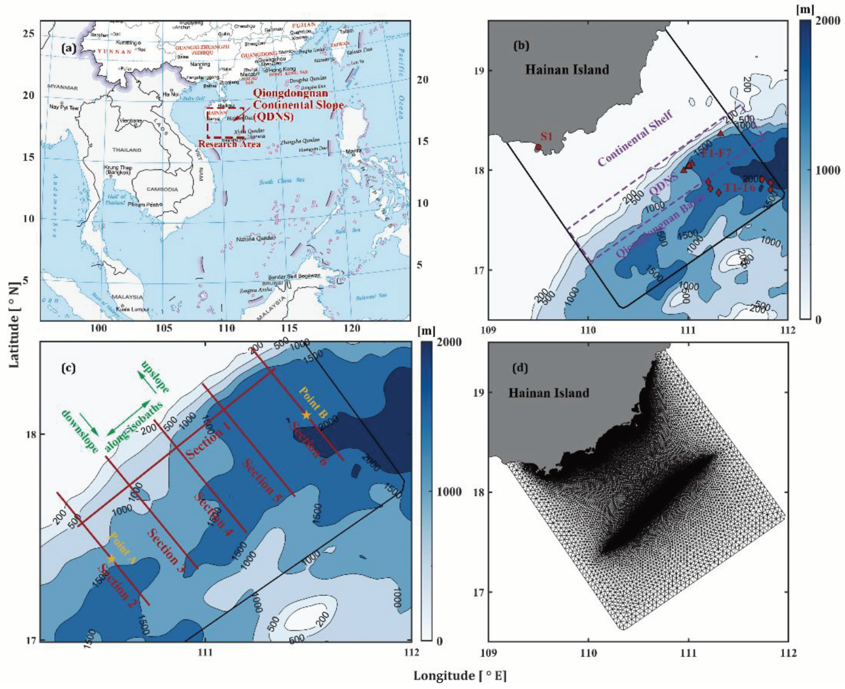
This study employs an unstructured grid, Finite Volume Coastal Ocean Model (FVCOM) [28], to simulate the three-dimensional, time-dependent circulation in the QDNS of the northern SCS at a relatively short temporal resolution of days to weeks. The unstructured triangular grid provides high flexibility and variability, which ensures high spatial resolution model results by giving a small-sized grid in the key study areas such as QDNS in this paper. Using a finite-volume approach, FVCOM is well-suited to maintain mass, momentum, temperature, and salinity conservation over complex topography such as QDNS, improving the calculation accuracy of the transport fluxes of water, heat and salt. The model can be run in two distinct modes using the model-split solver: an external mode which solves the vertically integrated (two-dimensional) equations of motion and an internal mode which resolves the three-dimensional structure.

2.1.1. Model Domain

The model domain of about 42,315 km2 is bounded by Hainan Island at the land side and exhibits an open boundary at the sea side, indicated by the solid black line in Figure 1b. Figure 1d depicts the unstructured triangular grid of the numerical model, which contains 24,889 nodes and 48,792 cells. The size of a horizontal grid cell is about 5000 m along the open boundary and gradually decreases to about 200 m in the QDNS and nearshore area to resolve short-term slope-induced hydrodynamics (Figure 1d). Vertically, for the internal mode, the model employs a hybrid, terrain-following coordinate system consisting of 40 layers to match the complex bathymetry between the continental shelf area and the Qiongdongnan basin (Figure 1b). Precisely, for sea floor locations with a depth of less than 80 m, these layers are evenly spaced, whereas for sea floor locations with a depth of more than 80 m, the near-floor and near-free-surface layers are more densely spaced (5 layers with a 2 m spacing) than those in between.
Coastline data is obtained from the Global Self-consistent, Hierarchical, High-resolution Geography Database (GSHHG) produced by the National Geophysical Data Center (NGDC) [29]. Topography is constructed based on the NGDC’s ETOPO1 Global Relief Model [30], with 1° resolution in longitude-latitude.

2.1.2. Model Configurations

The model run covers the time from 15 June to 1 October 2020. The first 16 days of the total simulation period are used to reach a quasi-equilibrium, and the remaining 92 days for analysis. The time step used in the external mode of the FVCOM is 1 s, which is bounded through the Courant–Friedrich Levy (CFL) stability criterion [31], while the time step of the internal mode is 5 s. Hourly output results ensure the high temporal precision needed to resolve the short-term ocean dynamics in the QDNS.
The model is forced with initial, open boundary and free surface conditions, but cold-started with zero tidal elevation and flow velocity. We initialized thermohaline conditions using the Global Ocean Forecasting System (GOFS 3.1) of the HYbrid Coordinate Ocean Model (HYCOM) [32]. The database has a horizontal resolution of 1/12° in both longitude and latitude, a vertical resolution of 41 layers, and a temporal frequency of 3 h.
Active open boundary conditions are applied to integrate external tidal and thermohaline forces. Hourly tidal elevations along the open boundary were predicted by 13 harmonic components (K1, O1, P1, Q1, M2, S2, N2, K2, M4, MS4, MN4, Mf, Mm) from the TPXO 7.2 global tide Model [33]. The external forcing of the thermohaline variables along the open boundary is also provided by HYCOM, GOFS 3.1 [32].
The free surface is forced by climatological wind stress and atmospheric heat flux, calculated from the u/v-wind component (0.2° × 0.2°) 10 m above the ground and air-sea interface thermal parameters (0.2° × 0.2°), including latent heat flux, sensible heat flux, downward shortwave radiation flux, upward shortwave radiation flux, downward longwave radiation flux and upward longwave radiation flux at the water surface, respectively. Both wind and heat flux data are derived from the National Centers for Environmental Prediction (NCEP) Climate Forecast System Version 2 (CFSv2) [34]. The relevant information on model forcing is organized in Table 1.

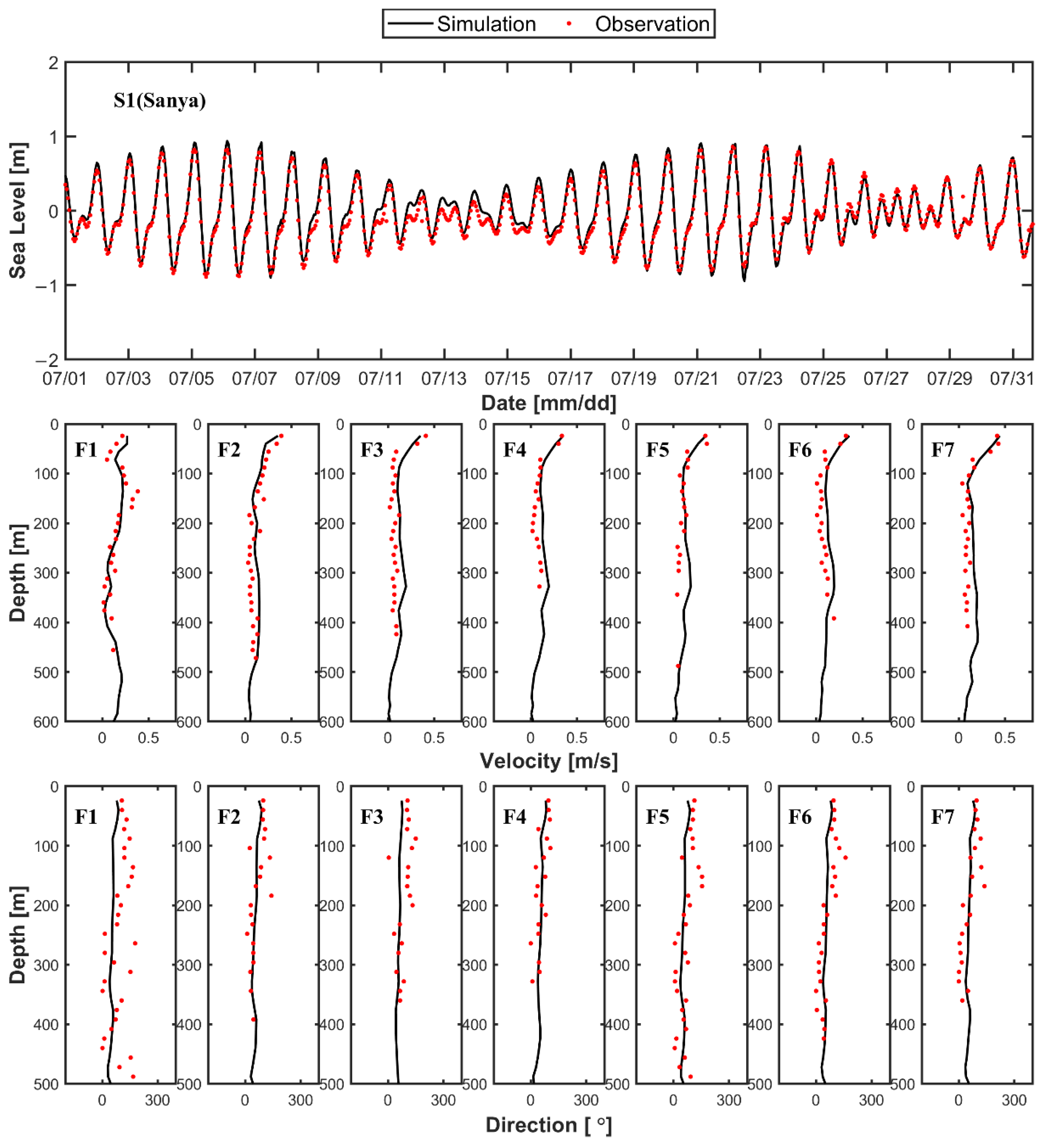
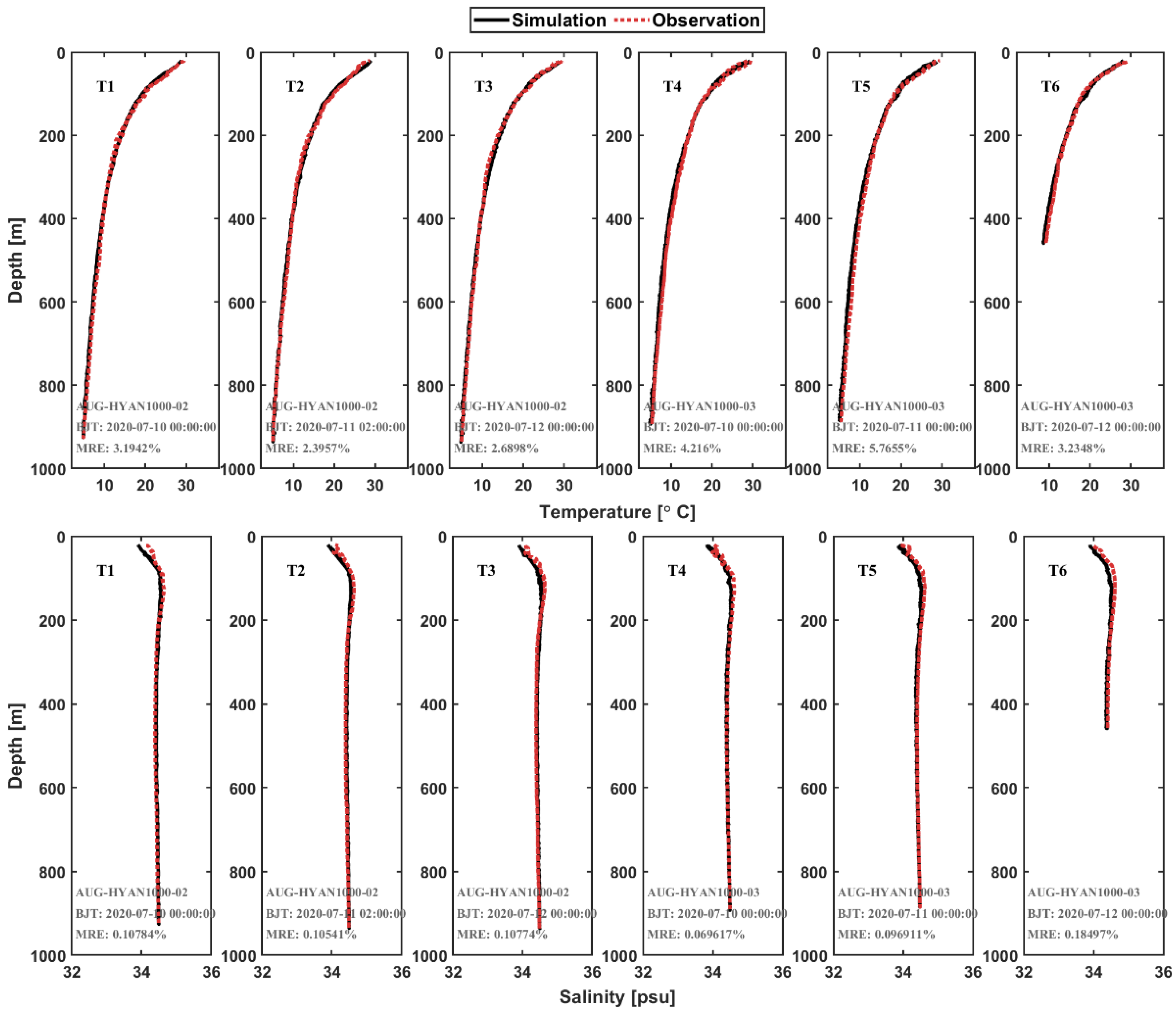
2.1.3. Model Validation

We calibrate the model outputs of sea level, flow velocity and direction, temperature, and salinity using the correlation coefficient ( C C ), the Willmott skill score ( W S S ), and mean relative error ( M R E ):
C C = 1 N i = 1 N ( m i m ¯ ) ( O i O ¯ ) S m S o ,  
W S S = 1 i = 1 N | m i O i | 2 i = 1 N ( | m i O ¯ i | + | O i O ¯ i | ) 2 ,
M R E = 1 N i = 1 N | m i O i | O i × 100 %   ,
where m i represents the simulation results, and O i refers to the observation results. m ¯ ( S m ) and O ¯ ( S o ) are the average values (standard deviations) of the calculated and observed values, respectively. W S S and C C values close to unity mean a significant correlation between the numerical simulation and field observations [35].
Figure 2 compares the simulation results (black lines) with the reference data (red dots) for July 2020, provided by the Sanya tide gauge (109°30′ E, 18°14′ N) and collected by the vessel-mounted Acoustic Doppler Current Profiler (ADCP) during a hydrographic survey conducted in the summer of 2020. The survey also provides several thermohaline profiles data collected by two glider-mounted Conductivity, Temperature, Depth (CTD) sensors, which are used to calibrate the temperature and salinity field in the model (Figure 3). The sea level, flow, and thermohaline validate stations are indicated by the red dot, triangles and diamonds, respectively, in Figure 1b.
It can be seen that the distribution and magnitude of the simulation data are consistent with the measurements, suggesting that the model can adequately simulate the flow, sea level, and thermohaline characteristics of the study area. This is supported by C C and W S S values close to unity for the sea level and flows and small MREs for temperature and salinity (Table 2). Note that the flow, temperature and salt validation are based on short-term measurements, supporting that the FVCOM model can be applied to study the short-term slope dynamics in the QDNS.

2.2. Thermohaline Balance

The instantaneous rate of transport of salt through a unit width of a section perpendicular to the mean flow is given by Dyer [36]
Q = 0 h u s   d z = h u s ,
where h is the depth and s is the salinity. At any depth, one can separate u and s via
{ u = u z + u , s = s z + s ,
where u z and s z are the observed values averaged over an hour, and u and s are their turbulent variations. u z and s z may be further separated into mean and deviation with respect to the depth averaging procedure:
{ u z = u + u v , s z = s + s v ,
{ u = 1 h 0 h u z   d z = u ¯ + U , s = 1 h 0 h s z   d z = s ¯ + S ,
where u v and s v are the depth deviations from the depth averaged values u and s . Because of tidal fluctuations, u and s will fluctuate greatly over a tidal cycle. Consequently, separating into mean and fluctuation with respect to a time-averaging procedure yields u = u ¯ + U and s = s ¯ + S , and
{ u ¯ = 1 T 0 T u   d t , s ¯ = 1 T 0 T s   d t ,
where U and S are the tidal cycle time fluctuations of the tidal cycle mean values u ¯ and s ¯ . Putting everything together yields
Q ¯ = h ¯ u ¯ s ¯ + 1 T 0 T h U S   d t + 1 T 0 T h u V s V d t + 1 T 0 T h u s d t = h ¯ u ¯ s ¯ + ( h U S ¯ ) + h u v s v ¯ + h u s ¯ = Q 1 + Q 2 + Q 3 + Q 4 ,
where the brackets denote the depth average of the products u v s v and u s , and h ¯ is the mean depth. The first term Q 1 represents the contribution to the total salt flux by the Eulerian mean flow. The second term Q 2 , generally known as tidal pumping, occurs when the tide does not act as a purely standing wave. The third term Q 3 arises from the velocity and salinity variation with depth, the shear effect, and will be finite if the two are correlated. Q 3 can also be termed a gravitational mode and includes the effect of vertical diffusion. The fourth term Q 4 represents the salt flux owing to the short period of turbulence. We neglect this term because it is usually much smaller than the other terms [36].
The heat balance equation is similar to the salt balance equation introduced above, except that the parameter s is replaced by ρ C p t , where t is the temperature, ρ is the water density, and C p = 4168   J / k g ° C is the specific heat capacity.

3. Results and Discussions

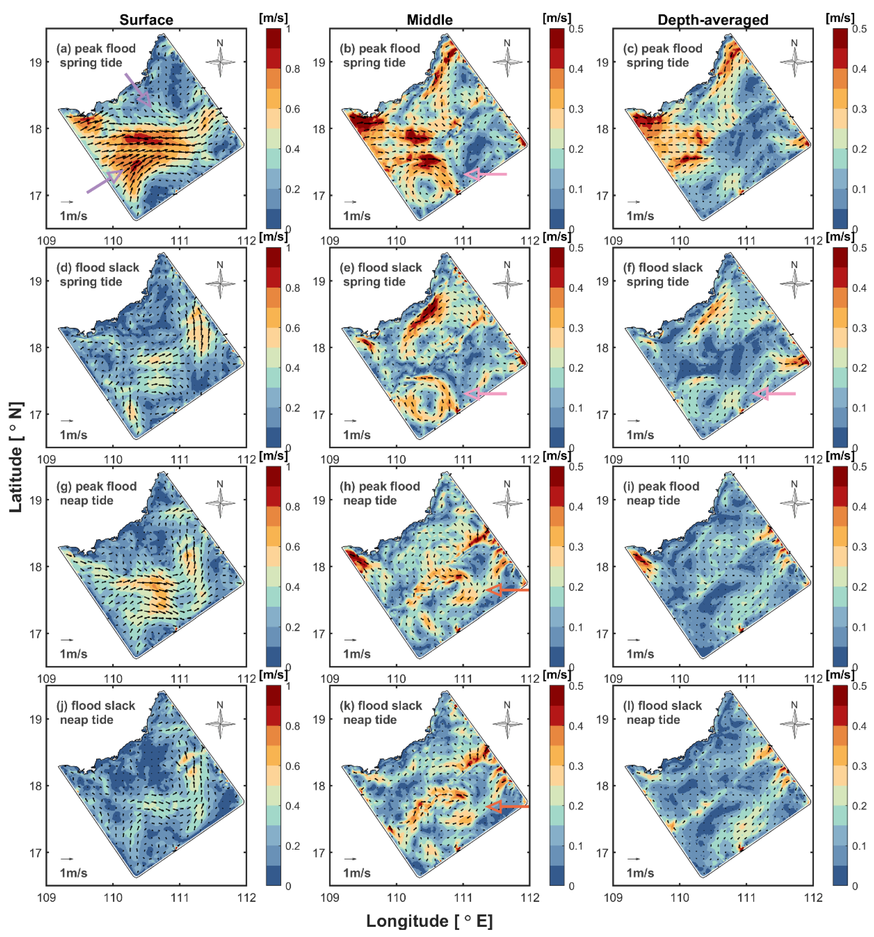
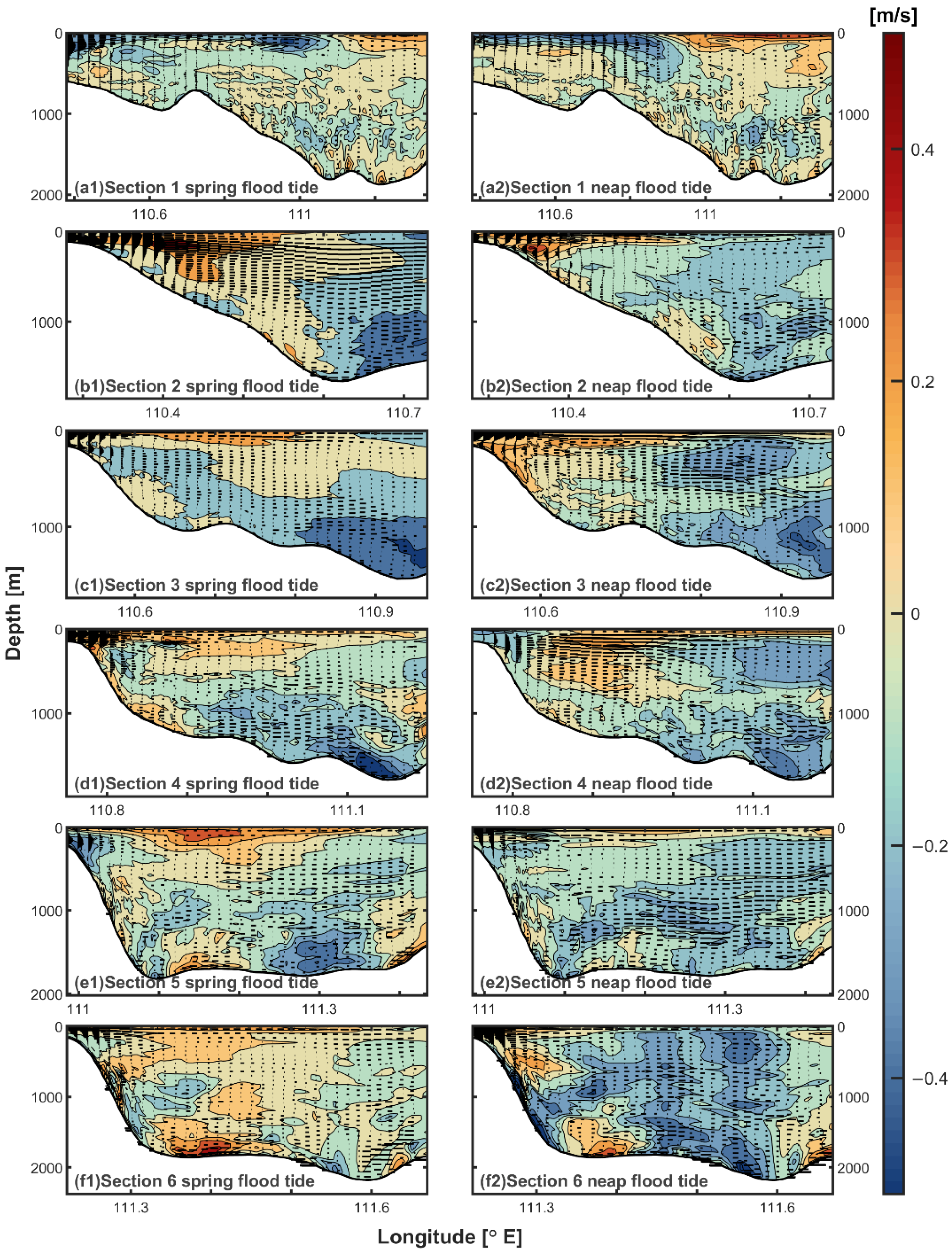
3.1. Hydrodynamic Structure

In order to study the short-term dynamics in the QDNS, we analyzed the flow field in the research area at two characteristic moments (i.e., peak flood and flood slack), with focus on the similarities and differences of the flow field between the spring tide and neap tide periods.
At peak flood, the flow field exhibits the following characteristics: (i) a strong influx of surface water at the entire western open boundary, (ii) a strong overall influx of water from both open boundaries in the continental shelf area due to strong flows in the middle (and lower) water layers, and (iii) a strong surface flow along the isobaths in the basin area directed northeastward (Figure 4). These features are much more pronounced during the spring tide (Figure 4a–c) than during the neap tide (Figure 4g–i). At flood slack, the flow in the basin area remains, but not at the same strength, whereas the flow in the continental shelf area no longer exhibits a clear characteristic.
A cyclonic eddy distinctly exists during the spring tide within the areas between 110° N to 110.8° E, and 16.8° N to 17.6° N, which is indicated by the pink arrow in Figure 4b,e,f. The eddy moves northeastward from the spring tide (shown by the pink arrow in Figure 4b,e) to the neap tide (shown by the orange arrow in Figure 4h,k), with a substantially reduced maximum velocity (from 0.7 m/s to 0.3 m/s).
Considering the complex topography of the QDNS, six representative sections are chosen for presenting the vertical flow structure (Figure 1c). Section 1 in Figure 1c is approximately directed along the isobaths of the QDNS, while Sections 2–6 are perpendicular to Section 1 in the downslope direction. Contours and arrows in Figure 5 depict the water flow velocities across and along these sections, respectively, at two characteristic instances. It can be seen that the water flows upslope east of 111.1° E and downslope west of 111.1° E during the spring tide (Figure 5a1). Water flow across the isobath mainly occurs at depths of less than 200 m. The maximum value of the upslope flow velocity increases from 0.2 m/s (Figure 5a1) to 0.4 m/s (Figure 5a2), indicating a stronger cross-isobaths water exchange during the neap tide than the spring tide. It can also be inferred from the cross-sectional flow velocity in Sections 2–6 that, along the isobaths, the surface water flows northeastward near the QDNS, while the bottom water flows southwestward in the basin area (Figure 5b–f).

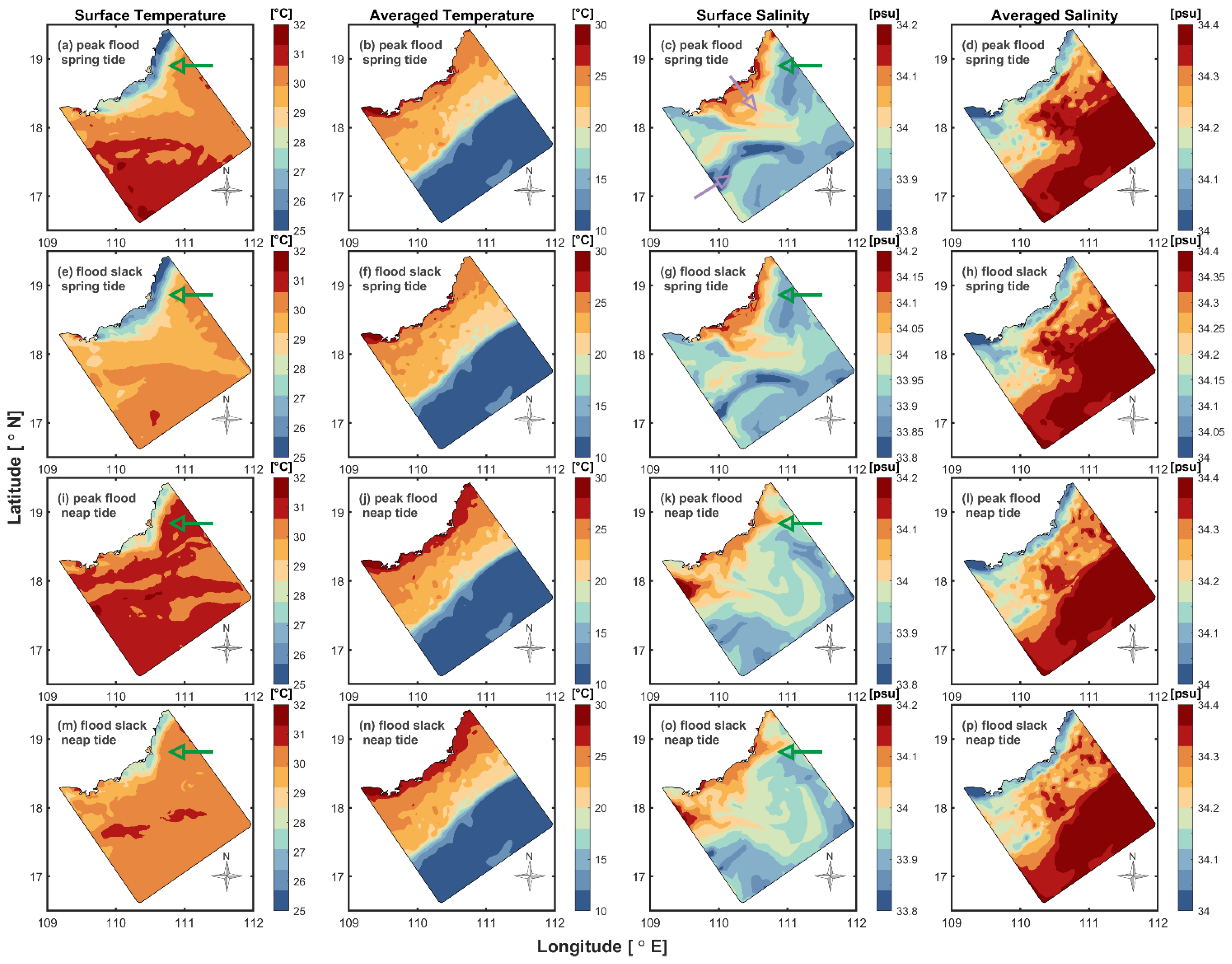
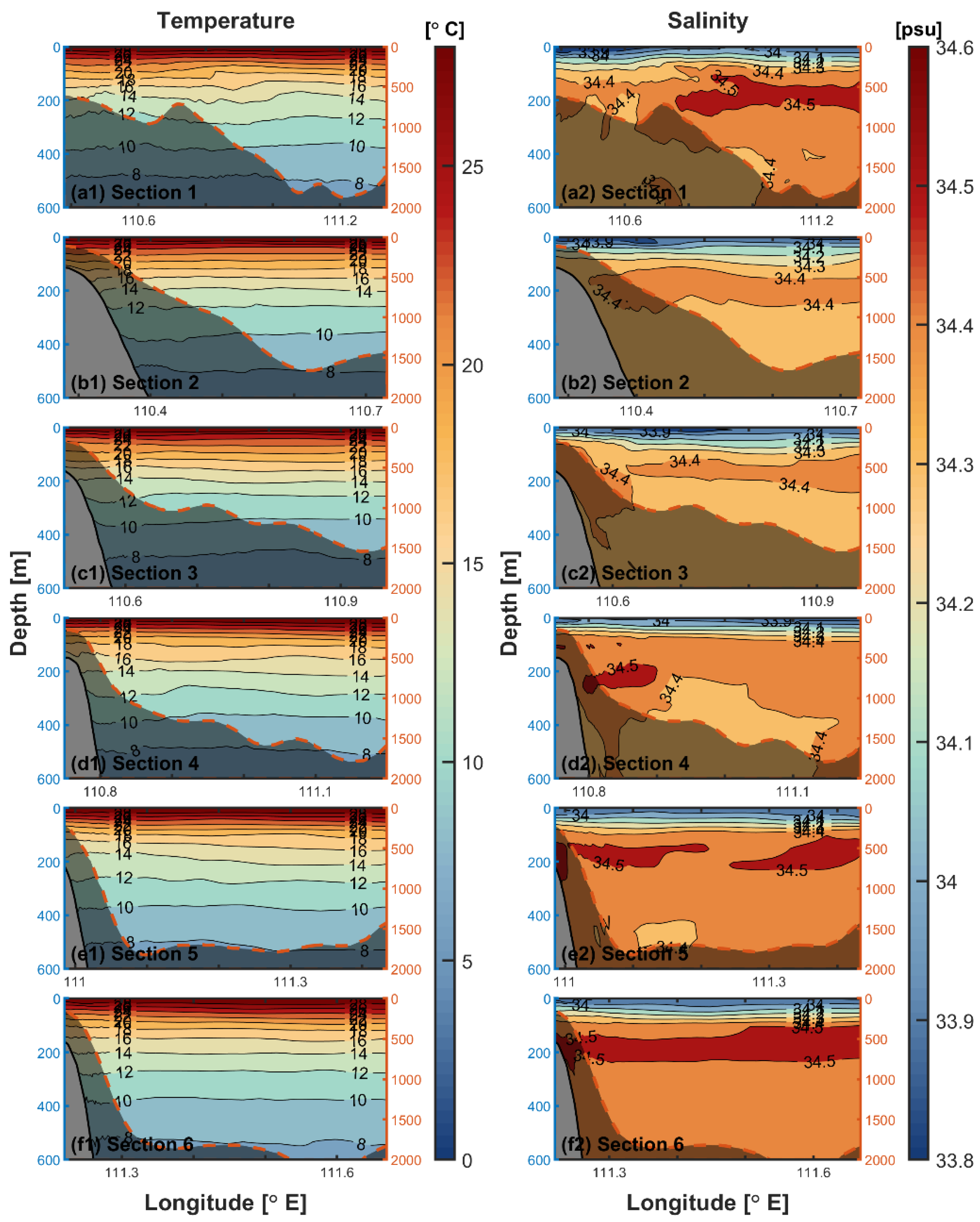
3.2. Thermohaline Structure

Qiongdong upwelling pumps the cold salt water from the seafloor upwards [2], influencing the distributions of the sea surface temperature (SST) and sea surface salinity (SSS) within the study area (Figure 6a,c). Compared with the basin area, the SST near the coast of Hainan Island, indicated by the green arrow, is lower by 5 °C while salinity is higher by 0.3 psu. This result is consistent with reports by Jing et al. [1] and Bai et al. [37]. Outside the coastal upwelling area, the SST in the model domain is approximately 30 °C, except at peak flood of the neap tide when temperatures rise to 32 °C because of peaking air-sea heat flux (Figure 6i). This implies that SST is temporally associated with air-sea heat flux.
The SSS distributions in Figure 6c,g,k,o are strongly spatially correlated with the surface flow field in Figure 4a,d,g,j, suggesting that advection contributes to salt transport. As the lilac arrows in Figure 4a and Figure 6c show, the flow comes from the southwest open boundary and the Qiongdong upwelling area brings fresh and salt water, respectively. Thus, the SSS on the left side of Section 1 in Figure 1c differs from that on the right side (Figure 7a2). Vertically, the halocline appears at 100~250 m. In the along-isobaths direction, the halocline east of 110.8° E is thicker and saltier than that of the west (Figure 7a2). In contrast, Sections 2–6 presented a weaker spatial distinction of the halocline in the along-section direction.

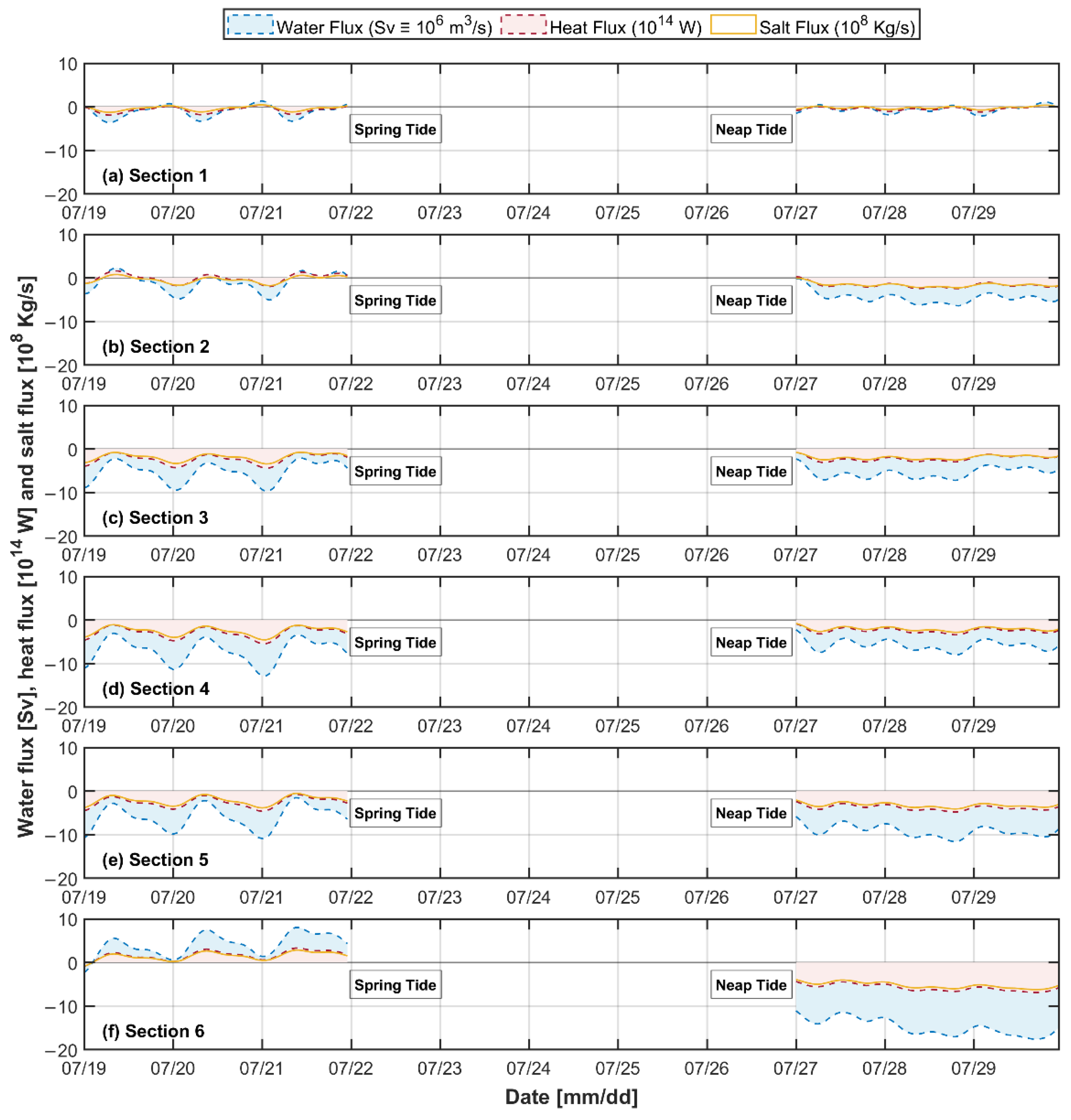
3.3. Water, Heat, and Salt Fluxes

The water ( W f ), heat ( H f ), and salt ( S f ) fluxes can be calculated as [38]
W f = 0 x h 0 u d z d x ,
H f = 0 x h 0 ρ C p u T d z d x ,
S f = 0 x h 0 ρ u S d z d x
where u represents the cross-sectional flow velocity component, h is the water depth, x the section width, ρ the density of water, and C p = 4168   J / k g ° C the specific heat capacity.
Table 3 shows the net water/heat/salt transport across Sections 1–6 of Figure 1c, calculated by numerical integration of the water/heat/salt flux curves shown in Figure 8. In Section 1, the water flux peaks at −3.59 Sv at UTC 2020-07-19 07:00 (i.e., the peak flood of the spring tide) when the flow velocity reached its maximum value. The negative values of the water volume transport across Section 1 during the spring tide (−2.86 × 10¹¹ m3) and neap tide (−1.31 × 10¹¹ m3) indicate a residual current in the downslope direction (Table 3).
The net water fluxes are negative in Sections 2–6 (except for Section 6 during the spring tide), demonstrating that water flows southwestward in the along-isobaths direction of the QDNS (Figure 8b–f). Considering our previous conclusion (Section 3.1) that the surface water flows northeastward near the QDNS, while the bottom water flows in the direction opposite to it in the basin area, we can now deduce that the net water transport in the along-isobaths direction of the QDNS is dominated by the southwestward bottom water in the basin area. Similar behavior can be seen in the hydro-thermohaline curves (Figure 8b–f), but the water, heat, and salt transports during the neap tide gradually increase from Section 2 to Section 6 (Table 3) due to increasing averaged water depth.
The water, heat, and salt transports across Section 6 during the spring tide are 1.08 × 10¹² m3, 4.44 × 10¹⁴ W, and 3.81 × 10¹³ kg, respectively. This anomaly can be understood when taking a look at the flow variations of Points A and B in Figure 1c (yellow stars). In fact, during the neap tide, the depth-averaged flow velocity there is negative (Figure 9c) due to the dominant southwestward flow (Figure 4i). During the spring tide, the eddy discussed in Section 3.1 causes a constantly changing flow direction at Point B (red lines in Figure 9b,c). In contrast, the flow at Point A (black lines in Figure 9b,c), which is not covered by the eddy, is dominated by the surface current, resulting in a positive depth-averaged velocity. As discussed, the northeastward water, heat, and salt transports during the spring tide in Section 6 can be attributable to the eddy.
The quantitative calculation of the net transport fluxes leads to the following conclusions. Spatially, hydro-thermohaline transport in the downslope direction (Section 1) is typically smaller than those along the isobaths (Sections 2–6). Temporally, the spring tide makes a 119%/70%/120% higher contribution to water/heat/salt transport than the neap tide in Section 1. In Sections 2–6, the net water/heat/salt transported during the spring tide was generally smaller (i.e., 38%/38%/38% on average) than that during the neap tide (Figure 10).

3.4. Thermohaline Balance

As discussed above, we have established a strong correlation between the spatial distributions and cross-sectional transport fluxes of water and salt. In this section, we discuss the mechanisms by which the water flow affects the salinity as well as the temperature. Based on the thermohaline balance equation introduced in Section 2.2, Figure 11 and Figure 12 show the hydrodynamic terms contributing to salt and heat fluxes, respectively, where 16-days-averaged simulation results from 14 July to 29 July 2020 have been used for the calculation.
The Eulerian mean flow term ( Q 1 ) contributes the majority of the overall salt flux (~±5 m2/s) and heat flux (~±5 × 10⁹ Jm−1 s−1). In contrast, the magnitude of the tidal pumping term ( Q 2 ) was only one-thousandth of Q 1 , indicating a negligible effect on heat and salt transports in the study domain. The Gravitational Convection term ( Q 3 ) is two orders of magnitude smaller than Q 1 for salt transport. However, for heat transport, Q 3 has the same magnitude as Q 1 (Figure 12), explaining why the correlation between the water and salt fluxes is much stronger than between the water and heat fluxes.
In Section 1 of Figure 1c, Q 1 constitutes a negative (downslope) contribution to the thermohaline flux west of 110.9° E and a positive (upslope) one east of it (Figure 11a and Figure 12a), similar to the flow velocity distribution in Figure 5a1. Q 3 has the same effect as Q 1 on the heat flux but the opposite effect on the salt flux. East of 110.9° E, Q 3 contributes a maximum of 8.12 × 10⁹ Jm−1 s−1 to the heat flux, more than three times of the maximum Q 1 .
In Sections 2–6, Q 3 contributes significantly to the northeastward heat flux, with a maximum value up to 1010 Jm−1 s−1 (Figure 12). Q 3 has the same effect as Q 1 on the salt flux but the opposite effect on the heat flux.

4. Conclusions

The hydro-thermohaline environment in the QDNS of the SCS has been investigated using the well-established FVCOM model. This study reports the short-term spatial-temporal behavior of the hydro-thermohaline characteristics and transport fluxes of water, heat and salt in the QDNS during tide cycles. The mechanisms responsible for them are studied by comparing different terms in the thermohaline balance equation.
The surface water near the QDNS moves northeastward along the isobaths, while the bottom water in the basin area, which dominates the net flux of the water transport, moves southwestward. In the downslope direction, water, heat, and salt transports during the spring tide are substantially larger (119%, 70% and 120% higher, respectively) than during the neap tide, while the opposite is true (62%, 62% and 62% lower, respectively) for transports along the isobaths. A stronger cross-isobaths water exchange during the neap tide is responsible for the former, while the latter is caused by dominating southwestward flow and the motion of a subsurface cyclonic eddy. Moreover, salt transport generally strongly correlates with water transport since the mean flow dominates the salt balance equation. In addition, for heat transport, gravitational convection also plays a substantial role in the heat balance, weakening the correlation between transports of heat and water.
The data of the short-term thermohaline evolution of the QDNS provided in this study may be of use for future studies of the northern SCS, including its marine ecology environment protection, marine pollution prevention, and ocean ranching development.

Author Contributions

Conceptualization, Z.H. and L.L.; methodology, L.L.; software, W.H.; validation, W.H.; formal analysis, W.H. and T.P.; investigation, W.H.; resources, J.L.; data curation, W.H.; writing—original draft preparation, Z.H. and W.H.; writing—review and editing, T.P. and L.L.; visualization, W.H.; supervision, Z.H. and L.L.; project administration, Z.H. and L.L.; funding acquisition, Z.H. and L.L. All authors have read and agreed to the published version of the manuscript.

Funding

This research was funded by the National Key Research and Development Program of China: No. 2021YFE0206200; National Key Research and Development Program of China: No. 2017YFC0305905; Key Research and Development Project of Hainan Province: No. ZDYF2022SHFZ045.

Institutional Review Board Statement

Not applicable.

Informed Consent Statement

Not applicable.

Data Availability Statement

Not applicable.

Acknowledgments

We appreciate Samuel Ukpong Okon’s comments on the manuscript and the formatting of the figures.

Conflicts of Interest

The authors declare no conflict of interest.

References

  1. Jing, Z.; Qi, Y.; Hua, Z.; Zhang, H. Numerical study on the summer upwelling system in the northern continental shelf of the south china sea. Cont. Shelf Res. 2009, 29, 467–478. [Google Scholar] [CrossRef]
  2. Wang, D.; Yang, Y.; Wang, J.; Bai, X. A modeling study of the effects of river runoff, tides, and surface wind-wave mixing on the eastern and western hainan upwelling systems of the south china sea, china. Ocean Dyn. 2015, 65, 1143–1164. [Google Scholar] [CrossRef]
  3. Li, Y.; Peng, S.; Wang, J.; Yan, J.; Huang, H. On the mechanism of the generation and interannual variations of the summer upwellings west and southwest off the hainan island. J. Geophys. Res. Ocean. 2018, 123, 8247–8263. [Google Scholar] [CrossRef]
  4. Fan, W.; Song, J.; Li, S. A numerical study on seasonal variations of the thermocline in the south china sea based on the roms. Acta Oceanol. Sin. 2014, 33, 56–64. [Google Scholar] [CrossRef]
  5. Johari, A.; Akhir, M.F. Exploring thermocline and water masses variability in southern south china sea from the world ocean database (wod). Acta Oceanol. Sin. 2019, 38, 38–47. [Google Scholar] [CrossRef]
  6. Chen, G.; Hou, Y.; Chu, X. Mesoscale eddies in the south china sea: Mean properties, spatiotemporal variability, and impact on thermohaline structure. J. Geophys. Res. 2011, 116, C06018. [Google Scholar] [CrossRef]
  7. Chen, G.; Gan, J.; Xie, Q.; Chu, X.; Wang, D.; Hou, Y. Eddy heat and salt transports in the south china sea and their seasonal modulations. J. Geophys. Res. Ocean. 2012, 117, C05021. [Google Scholar] [CrossRef]
  8. Li, D. Analysis of Water Masses in the Continental Slope of the Northern South China Sea; Shanghai Jiao Tong University: Shanghai, China, 2017. [Google Scholar]
  9. Lopes, P.F.M.; Verba, J.T.; Begossi, A.; Pennino, M.G. Predicting species distribution from fishers’ local ecological knowledge: A new alternative for data-poor management. Can. J. Fish. Aquat. Sci. 2019, 76, 1423–1431. [Google Scholar] [CrossRef]
  10. Falardeau, M.; Bennett, E.M.; Else, B.; Fisk, A.; Mundy, C.J.; Choy, E.S.; Ahmed, M.M.M.; Harris, L.N.; Moore, J.-S. Biophysical indicators and indigenous and local knowledge reveal climatic and ecological shifts with implications for arctic char fisheries. Glob. Environ. Chang. 2022, 74, 102469. [Google Scholar] [CrossRef]
  11. Muringai, R.T.; Mafongoya, P.L.; Lottering, R. Climate change and variability impacts on sub-saharan african fisheries: A review. Rev. Fish. Sci. Aquac. 2021, 29, 706–720. [Google Scholar] [CrossRef]
  12. Cai, M.; He, H.; Liu, M.; Li, S.; Tang, G.; Wang, W.; Huang, P.; Wei, G.; Lin, Y.; Chen, B.; et al. Lost but can’t be neglected: Huge quantities of small microplastics hide in the south china sea. Sci. Total Environ. 2018, 633, 1206–1216. [Google Scholar] [CrossRef]
  13. Zhu, L.; Wang, H.; Chen, B.; Sun, X.; Qu, K.; Xia, B. Microplastic ingestion in deep-sea fish from the south china sea. Sci. Total Environ. 2019, 677, 493–501. [Google Scholar] [CrossRef]
  14. Kuo, Y.; Tseng, Y. Impact of enso on the south china sea during enso decaying winter–spring modeled by a regional coupled model (a new mesoscale perspective). Ocean Model. 2020, 152, 101655. [Google Scholar] [CrossRef]
  15. Xie, J.; He, Y.; Cai, S. Bumpy topographic effects on the transbasin evolution of large-amplitude internal solitary wave in the northern south china sea. J. Geophys. Res. Ocean. 2019, 124, 4677–4695. [Google Scholar] [CrossRef]
  16. Li, W.; Alves, T.M.; Wu, S.; Völker, D.; Zhao, F.; Mi, L.; Kopf, A. Recurrent slope failure and submarine channel incision as key factors controlling reservoir potential in the south china sea (qiongdongnan basin, south hainan island). Mar. Pet. Geol. 2015, 64, 17–30. [Google Scholar] [CrossRef]
  17. Estrade, P.; Marchesiello, P.; De Verdière, A.C.; Roy, C. Cross-shelf structure of coastal upwelling: A two-dimensional extension of ekman’s theory and a mechanism for inner shelf upwelling shut down. J. Mar. Res. 2008, 66, 589–616. [Google Scholar] [CrossRef]
  18. Chen, Z.; Yan, X.; Jiang, Y.; Jiang, L. Roles of shelf slope and wind on upwelling: A case study off east and west coasts of the us. Ocean Model. 2013, 69, 136–145. [Google Scholar] [CrossRef]
  19. Jacox, M.G.; Edwards, C.A. Effects of stratification and shelf slope on nutrient supply in coastal upwelling regions. J. Geophys. Res. 2011, 116, C03019. [Google Scholar] [CrossRef]
  20. Oke, P.R.; Middleton, J.H. Topographically induced upwelling off eastern australia. J. Phys. Oceanogr. 2000, 30, 512–531. [Google Scholar] [CrossRef]
  21. Su, J.; Pohlmann, T. Wind and topography influence on an upwelling system at the eastern hainan coast. J. Geophys. Res. 2009, 114, C06017. [Google Scholar] [CrossRef] [Green Version]
  22. Gan, J.; Liu, Z.; Hui, C.R. A three-layer alternating spinning circulation in the south china sea. J. Phys. Oceanogr. 2016, 46, 2309–2315. [Google Scholar] [CrossRef]
  23. Xu, F.-H.; Oey, L.-Y. State analysis using the local ensemble transform kalman filter (letkf) and the three-layer circulation structure of the luzon strait and the south china sea. Ocean Dyn. 2014, 64, 905–923. [Google Scholar] [CrossRef]
  24. Zhang, Z.; Zhao, W.; Tian, J.; Liang, X. A mesoscale eddy pair southwest of taiwan and its influence on deep circulation. J. Geophys. Res. Ocean. 2013, 118, 6479–6494. [Google Scholar] [CrossRef]
  25. Liu, C.; Li, X.; Wang, S.; Tang, D.; Zhu, D. Interannual variability and trends in sea surface temperature, sea surface wind, and sea level anomaly in the south china sea. Int. J. Remote Sens. 2020, 41, 4160–4173. [Google Scholar] [CrossRef]
  26. Zhang, H.; Cheng, W.; Chen, Y.; Yu, L.; Gong, W. Controls on the interannual variability of hypoxia in a subtropical embayment and its adjacent waters in the guangdong coastal upwelling system, northern south china sea. Ocean Dyn. 2018, 68, 923–938. [Google Scholar] [CrossRef]
  27. Daryabor, F.; Ooi, S.H.; Samah, A.A.; Akbari, A. Dynamics of the water circulations in the southern south china sea and its seasonal transports. PLoS ONE 2016, 11, e0158415. [Google Scholar] [CrossRef]
  28. Chen, C.S.; Liu, H.D.; Beardsley, R.C. An unstructured grid, finite-volume, three-dimensional, primitive equations ocean model: Application to coastal ocean and estuaries. J. Atmos. Ocean. Technol. 2003, 20, 159–186. [Google Scholar] [CrossRef]
  29. Wessel, P.; Smith, W.H.F. A global, self-consistent, hierarchical, high-resolution shoreline database. J. Geophys. Res. Solid Earth 1996, 101, 8741–8743. [Google Scholar] [CrossRef]
  30. Amante, C.; Eakins, B.W. Etopo1 1 arc-minute global relief model: Procedures, data sources and analysis. In NOAA Technical Memorandum NESDIS NGDC-24; Barry, E., Ed.; National Geophysical Data Center: Boulder, CO, USA, 2009. [Google Scholar] [CrossRef]
  31. Wang, J. Global linear stability of the two-dimensional shallow-water equations: An application of the distributive theorem of roots for polynomials on the unit circle. Mon. Weather. Rev. 1996, 124, 1301–1310. [Google Scholar] [CrossRef]
  32. Chassignet, E.P.; Hurlburt, H.E.; Smedstad, O.M.; Halliwell, G.R.; Hogan, P.J.; Wallcraft, A.J.; Baraille, R.; Bleck, R. The hycom (hybrid coordinate ocean model) data assimilative system. J. Mar. Syst. 2007, 65, 60–83. [Google Scholar] [CrossRef]
  33. Foreman, M.G.G.; Bennett, A.F.; Egbert, G.D. Topex/poseidon tides estimated using a global inverse model. J. Geophys. Res. Ocean. 1994, 99, 24821–24852. [Google Scholar] [CrossRef]
  34. Saha, S.; Moorthi, S.; Wu, X.; Wang, J.; Nadiga, S.; Tripp, P.; Behringer, D.; Hou, Y.-T.; Chuang, H.-Y.; Iredell, M.; et al. The ncep climate forecast system version 2. J. Clim. 2014, 27, 2185–2208. [Google Scholar] [CrossRef]
  35. Onken, R. Forecast skill score assessment of a relocatable ocean prediction system, using a simplified objective analysis method. Ocean Sci. 2017, 13, 925–945. [Google Scholar] [CrossRef]
  36. Dyer, K.R. Estuaries: A Physical Introduction; University of Plymouth: Plymouth, UK, 1997. [Google Scholar]
  37. Bai, P.; Gu, Y.; Li, P.; Wu, K. Modelling the upwelling off the east hainan island coast in summer 2010. Chin. J. Oceanol. Limnol. 2016, 34, 1358–1373. [Google Scholar] [CrossRef]
  38. He, Q.; Zhan, H.; Cai, S.; He, Y.; Huang, G.; Zhan, W. A new assessment of mesoscale eddies in the south china sea: Surface features, three-dimensional structures, and thermohaline transports. J. Geophys. Res. Ocean. 2018, 123, 4906–4929. [Google Scholar] [CrossRef]
Figure 1. (a) Map showing the location of the QDNS and its adjacent seas. (b) Bathymetry of the research area in the northern SCS, where the black line defines the model domain. The red dot S1 (triangles F1–F7) indicates the sea level (flow) validation station, while thermohaline validation points T1-T6 are marked as red diamonds. (c) Bathymetry of the zoomed-in area around the QDNS. The red lines indicate six representative sections, the yellow stars indicate two represent points A and B, and the green arrows mark the downslope, upslope and along-isobaths direction. (d) The unstructured triangular grid of the numerical model.
Jmse 10 01221 g001
Figure 2. Model validation of sea level (upper), flow velocity (middle), and flow direction (lower).
Jmse 10 01221 g002
Figure 3. Model validation of temperature (upper) and salinity (lower).
Jmse 10 01221 g003
Figure 4. Flow field at different times and different layers. (ac) Peak flood of the spring tide. (df) Flood slack of the spring tide. (gi) Peak flood of the neap tide. (jl) Flood slack of the neap tide. (a,d,g,j) Sea surface flow field. (b,e,h,k) Middle layer flow field. (c,f,i,l) Depth-averaged flow field.
Jmse 10 01221 g004
Figure 5. Distribution of flow velocity in Sections 1–6 of Figure 1c. The left and right columns represent peak flood of the spring tide (UTC 2020-07-19 07:00) and the neap tide (UTC 2020-07-28 06:00), respectively. Contours show the magnitude of the cross-sectional flow velocity, where positive values represent water inflow and negative values represent water outflow. The direction and length of arrows represent the direction and velocity, respectively, of the along-section water flow.
Jmse 10 01221 g005
Figure 6. Temperature and salinity field at different times. (ad) Peak flood of the spring tide. (eh) Flood slack of the spring tide. (il) Peak flood of the neap tide. (mp) Flood slack of the neap tide. The columns represent SST (a,e,i,m), vertically averaged temperature (b,f,j,n), SSS (c,g,k,o), and vertically averaged salinity (d,h,l,p).
Jmse 10 01221 g006
Figure 7. Distribution of temperature (left) and salinity (right) in Sections 1–6 of Figure 1c at peak flood of the spring tide (UTC 2020-07-19 07:00). The colors and contours indicate the magnitude of each parameter, whereas the overlaying grey shadow shows the bathymetry. The blue label indicates the water depth corresponding to the underlaying color and contour plot. The orange label indicates the water depth corresponding to the overlaying shadow plot.
Jmse 10 01221 g007
Figure 8. Water flux (blue area), heat flux (pink area), and salt flux (yellow line) in Sections 1–6 of Figure 1c during the spring tide (19–22 July) and neap tide (27–29 July). A positive value indicates mass transport into the section, while a negative value indicates mass transport out of the section.
Jmse 10 01221 g008
Figure 9. The time-dependent variation of (a) the sea level, (b) surface flow velocity, and (c) depth-averaged flow velocity during the spring tide and the neap tide. The black lines and arrows represent Point A at Section 6 of Figure 1c, while the red lines and arrows represent Point B at Section 2.
Jmse 10 01221 g009
Figure 10. Spatial-temporal behavior of the hydro-thermohaline transport in the QDNS. Spring tide and neap tide are abbreviated as ST and NT, respectively.
Jmse 10 01221 g010
Figure 11. The contribution of different hydrodynamic terms to the salt flux in Sections 1–6 of Figure 1c. In Section 1, positive (negative) values indicate upslope (downslope) salt transport. In Sections 2–6, positive (negative) values imply northeastward (southwestward) salt transport.
Jmse 10 01221 g011
Figure 12. The contribution of different hydrodynamic terms to the heat flux in in Sections 1–6 of Figure 1c. In Section 1, positive (negative) values indicate upslope (downslope) heat transport. In Sections 2–6, positive (negative) values imply northeastward (southwestward) heat transport.
Jmse 10 01221 g012
Table 1. Model forcing conditions and relevant sources.
Forcing ConditionForcing TypeSource
InitialTide0
Flow0
TemperatureHYCOM GOFS 3.1 [32]
SalinityHYCOM GOFS 3.1 [32]
Open boundaryTideTPXO 7.2 [33]
Flow0
TemperatureHYCOM GOFS 3.1 [32]
SalinityHYCOM GOFS 3.1 [32]
Free SurfacewindNCEP CFSv2 [34]
heat fluxNCEP CFSv2 [34]
Table 2. Validation results of sea level and flow.
W S S C C M R E   ( % )
Sea Level0.990.99
Flow0.810.77
Temperature- 3.58
Salinity- 0.11
Table 3. The water, heat, and salt fluxes in Sections 1–6 of Figure 1c.
UnitsSection 1Section 2Section 3Section 4Section 5Section 6
Max water flux (ST)×106 m3/s ≡ Sv−3.59−5.06−9.70−12.83−10.878.03
Max water flux (NT)×106 m3/s ≡ Sv−2.11−6.39−7.19−8.00−11.61−17.59
Net water transport (ST)×1011 m3−2.86−2.70−13.55−18.28−15.4410.78
Net water transport (NT)×1011 m3−1.31−11.79−14.24−15.07−23.88−38.50
Max heat flux (ST)×1014 W−1.89−1.98−4.40−5.42−4.593.30
Max heat flux (NT)×1014 W−1.18−2.45−3.07−3.39−4.82−6.87
Net heat transport (ST)×1019 J−1.92−0.11−5.93−7.55−6.634.44
Net heat transport (NT)×1019 J−1.13−4.36−5.70−6.30−9.89−15.06
Max salt flux (ST)×108 kg/s−1.26−1.78−3.42−4.53−3.842.84
Max salt flux (NT)×108 kg/s−0.74−2.25−2.54−2.83−4.10−6.22
Net salt transport (ST)×1013 kg−1.00−0.96−4.78−6.45−5.453.81
Net salt transport (NT)×1013 kg−0.46−4.16−5.03−5.32−8.44−13.61
Note: Positive values represent current inflow and negative values current outflow. Spring tide and neap tide are abbreviated as ST and NT, respectively.
Publisher’s Note: MDPI stays neutral with regard to jurisdictional claims in published maps and institutional affiliations.

