Bipolar Fuzzy Supra Topology via (Q-) Neighborhood and Its Application in Data Mining Process

Abstract

The aim of this study is to provide neighborhood structures in bipolar fuzzy supra topological space and to show the applicability of bipolar fuzzy supra topology to the medical diagnosis problem. Firstly, we give some properties related to bipolar fuzzy points and their neighborhood structure in bipolar fuzzy supra topological spaces. Then, we consider another important structure, “quasi-coincident”, in the case of bipolar fuzzy points and bipolar fuzzy sets. Then, we introduce the corresponding neighborhood structure called “Q-neighborhood system” by using the quasi-coincident relations. Furthermore, we also investigate the characterization of bipolar fuzzy supra topological space in terms of quasi-neighborhoods. Finally, we present a new method to solve medical diagnosis problems by using the bipolar fuzzy score function.

1. Introduction

Throughout the history of humanity, mankind has put forward various disciplines to produce solutions to problems. Over time, these disciplines have been divided into sub-disciplines by being handled through different aspects. Mathematics is one of the oldest disciplines that has shared this fate. Mathematics is separated into many sub-disciplines and has been used effectively to find solutions in different disciplines such as engineering, medicine, and the humanities, especially through the classical set theory approach. However, classical set theory is insufficient to produce an effective solution to all problems encountered.

The notion of fuzzy sets was given by Zadeh [1] in 1965. The theory of fuzzy sets is a generalization of classical set theory; fuzzy sets grade elements as belonging to a set. A fuzzy set A defined on the universal set U can be denoted as $A=\{<u,{\mu }_A\left(u\right)>|u\in U\}$. Here ${\mu }_A$ is a function of the form ${\mu }_A:U\to [0,1]$ and ${\mu }_A\left(u\right)$ is called the membership degree of an arbitrary element $u\in U$.

Intuitionistic fuzzy sets [2] were defined by adding the degree of non-membership to fuzzy sets. Thus, this concept helps solve broader, real-life problems. The intuitionistic fuzzy set considers membership and non-membership degrees during analysis. For instance, in the fuzzy set, the degree of sweetness is given in the interval [0, 1], while in an intuitionistic fuzzy set, the degree of sweetness (${\mu }_A:U\to [0,1]$) and the degree of non-sweetness (${\nu }_A:U\to [0,1]$) are added to handle more general problems. In intuitionistic fuzzy sets, we have ${\mu }_A\left(u\right)+{\nu }_A\left(u\right)\le 1$. Suppose that ${\mu }_A\left(u\right)=0.6$ and ${\nu }_A\left(u\right)=0.5$, we obtain $0.6+0.5\nleqq 1$, but ${\left(0.6\right)}^2+{\left(0.5\right)}^2\le 1$. We could not solve this kind of problem in an intuitionistic fuzzy set. Therefore, Pythagorean fuzzy sets [3] were defined, which are more general than intuitionistic fuzzy sets because of their ability to model using incoherent data. These sets are characterized by the condition that the sum of the squares of membership and non-membership grades is less than or equal to 1. Thus, the sum of membership and non-membership grades can exceed 1.

Table 1. Some fuzzy models.

Fuzzy  Models	Advantages
Fuzzy set [1]	It can study with imprecise data. ${\mu }_A\left(u\right)$
Intuitionistic fuzzy set [2]	It includes membership and nonmembership values. ${\mu }_A\left(u\right)+{\nu }_A\left(u\right)\le 1$
Pythagorean fuzzy set [3]	It is suitable when the sum of membership and the nonmembership grade is more than one. ${\left({\mu }_A\left(u\right)\right)}^2+{\left({\nu }_A\left(u\right)\right)}^2\le 1$
Bipolar fuzzy set [8]	It is appropriate the positive and negative aspects of a problem. ${\mu }_A^{+}:U\to [0,1]$ and ${\mu }_A^{-}:U\to [-1,0]$

summarizes the advantages of these structures. By continuing the generalizations of fuzzy sets (neutrosophic fuzzy sets [4], picture fuzzy sets [5], spherical fuzzy sets [6], Pythagorean fuzzy sets [3]), the definition of bipolar fuzzy set was given by Zhang [7]. Bipolar-valued fuzzy sets are an extension of fuzzy sets with bipolarity.

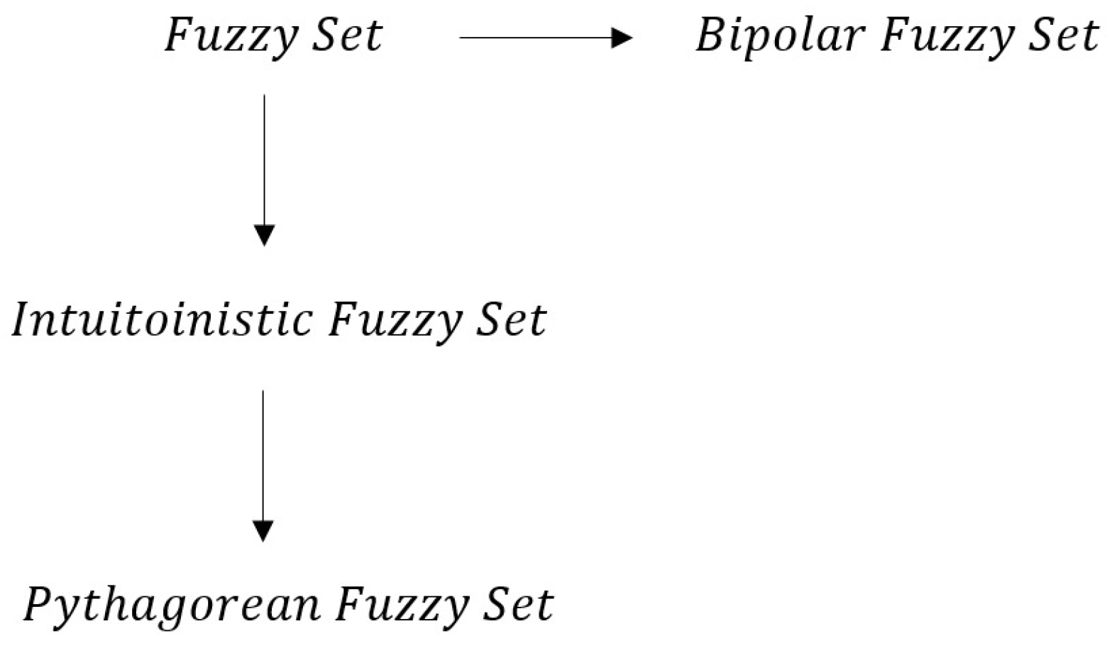
W.R. Zhang [7,9,10] extended the idea of a fuzzy set by introducing the concept of a bipolar fuzzy set. Bipolarity refers to the positive and negative facets of a problem. It is suitable for information containing a feature as well as its opposite, such as sourness and sweetness, competition and cooperation, happiness and grief. Although intuitionistic fuzzy sets and bipolar fuzzy sets appear parallel to each other, they are distinct sets. In comparison, we obtain ${\mu }_A^{+}\left(u\right)={\mu }_A\left(u\right)$ and ${\mu }_A^{-}\left(u\right)=-{\nu }_A\left(u\right)$, which look like similar to each other. However, in bipolar fuzzy sets, the positive membership degree (${\mu }_A^{+}\left(u\right)$) of a section shows that the section fairly fulfills the subject and the negative membership degree (${\mu }_A^{-}\left(u\right)$) of a section represents that the section fairly fulfills the implicit counter property. In intuitionistic fuzzy sets, the membership degree ${\mu }_A\left(u\right)$ represents the extent to which the element u satisfies property A, while the membership degree ${\nu }_A\left(u\right)$ signifies the degree to which u satisfies the not-property of A. Given that a counter property is distinct from a not-property, bipolar-valued fuzzy sets and intuitionistic fuzzy sets serve as distinct extensions of traditional fuzzy sets. Figure 1 summarizes the relation of them.

Recently, bipolar fuzzy sets have been utilized in various fields of research. Lee [8,11], defined bipolar fuzzy set operations and obtained their basic algebraic properties. Abdullah et al. [12] combined the bipolarity, fuzziness, and parameterization and gave the definition of bipolar fuzzy soft sets in 2014. They also gave an application of bipolar fuzzy soft set in decision-making problems. In 2019, Kim et al. [13] defined bipolar fuzzy points and studied the topological structures of bipolar fuzzy sets, such as neighborhood, base, continuity, product, and quotient spaces. In recent years, researchers have also studied the algebraic structures of bipolar fuzzy sets [14,15,16,17].

Chang [18] (1968) defined topological spaces on fuzzy sets and examined basic properties such as open-closed sets, continuity, and compactness. In 1976, Lowen [19] gave a new definition of fuzzy topology and guaranteed that the constant functions are continuous in fuzzy topological spaces in this sense. In Chang’s fuzzy topology, open sets are fuzzy, but the topology comprising those open sets is a subset of the family of fuzzy sets. Fuzzification of openness was first defined by Hohle [20] and later extended to L-subsets by Shostak [21]. Pao-Ming and Ying-Ming [22,23] defined the concept of a neighborhood of fuzzy points. They also brought out the structures of fuzzy quasi-coincident and Q-neighborhood. The fuzzy topology theory, which has been handled in many ways until today, has now reached a certain maturity. Topological structures of some extensions of fuzzy sets also have been studied. For example intuitonistic fuzzy topology [24], neutrosophic fuzzy topology [25,26], picture fuzzy topology [27], bipolar fuzzy topology [28], etc.

Supra topology [29] was defined by dropping a finite intersection condition of topological spaces. It is fundamental with respect to the investigation of classical topological spaces. Since then, many authors have studied supra topology and its extensions such as (intuitionistic) fuzzy supra topology [30,31,32]. In 2022, Hami et al. [33] discussed bipolar fuzzy supra topological spaces as a generalization of supra topologies to bipolar fuzzy topologies.

Neighborhood structures play important roles in (supra) topological spaces. As such, we aim to study neighborhood structures and related properties in bipolar fuzzy supra topological spaces. For this, this paper includes the following sections: In Section 2, we list basic definitions and results that are needed in the subsequent sections. In Section 3, we define the concept of neighborhood structure for a bipolar fuzzy point and generate a bipolar fuzzy supra-topology using the system of neighborhoods (see Theorem 11). The characterization of continuous mappings is also provided in this section. In Section 4, we introduce the concept of quasi-coincidence in bipolar fuzzy sets and obtain some of its properties. Subsequently, we study the Q-neighborhood structure of bipolar fuzzy supra-topological space. In the last section, we propose a method for data analysis within a bipolar fuzzy supra-topological environment as a real-life application, and we present numerical examples of the proposed method.

2. Preliminaries

In this section, we give some definitions and several results related to bipolar fuzzy sets.

Definition 1

([8]). Let U be a non-empty set. A bipolar fuzzy set A on U is an object having the form $A=\{<u,{\mu }_A^{+}\left(x\right),{\mu }_A^{-}\left(u\right)>:u\in U\}$ where ${\mu }_A^{+}:U\to [0,1]$ and ${\mu }_A^{-}:U\to [-1,0]$ are mappings. The positive membership degree ${\mu }_A^{+}\left(u\right)$ represents the satisfaction degree of an element u with respect to the property associated with a bipolar-valued fuzzy set A, while the negative membership degree ${\mu }_A^{-}\left(u\right)$ indicates the satisfaction degree of u with an implicit counter property of bipolar-valued fuzzy set A.

If ${\mu }_A^{+}\left(u\right)=0$ and ${\mu }_A^{-}\left(u\right)\ne 0$, it is the situation that u does not satisfy property of A but somewhat satisfies the counter property of A.

If ${\mu }_A^{+}\left(u\right)\ne 0$ and ${\mu }_A^{-}\left(u\right)=0$, it is the situation that u is regarded as having only positive satisfaction of A.

There are cases where the positive membership degree ${\mu }_A^{+}\left(u\right)$ and the negative membership degree ${\mu }_A^{-}\left(u\right)$ are both non-zero when the membership function of the property overlaps that of its counter property over certain elements in U.

The set of all bipolar fuzzy sets in U will be denoted as $BPF\left(U\right)$.

In the following, we give an example for bipolar fuzzy set.

Example 1.

Let $U=\{u,v,z\}$. $A=\{<u,0.6,-0.1>,<v,0.3,-0.3>,<z,0.4,-0.2>\}$ is a bipolar fuzzy set on U.

Definition 2

([28]). The empty bipolar fuzzy set is defined as $0^{+}\left(u\right)=0=0^{-}\left(u\right)$ , for each $u\in U$ and denoted by $\overline{0}=(0^{+},0^{-})$.

The whole bipolar fuzzy set is defined as $1^{+}\left(u\right)=1$ and $1^{-}\left(u\right)=-1$, for each $u\in U$ and denoted by $\overline{1}=(1^{+},1^{-})$.

With the following definition, we give the definitions of some set operations.

Definition 3

([34]). Let $A,B\in BPF\left(U\right)$. Then;

(1) $A\subseteq B$$:\iff$${\mu }_A^{+}\left(u\right)\le {\mu }_B^{+}\left(u\right)$ and ${\mu }_A^{-}\left(u\right)\ge {\mu }_B^{-}\left(u\right)$, for all $u\in U$.

(2) $A=B$$:\iff$${\mu }_A^{+}\left(u\right)={\mu }_B^{+}\left(u\right)$ and ${\mu }_A^{-}\left(u\right)={\mu }_B^{-}\left(u\right)$, for all $u\in U$.

(3) $A\cup B=\{<u,{\mu }_{A\cup B}^{+}\left(u\right),{\mu }_{A\cup B}^{-}\left(u\right)>:u\in U\}$, where ${\mu }_{A\cup B}^{+}\left(u\right)=max\{{\mu }_A^{+}\left(u\right),{\mu }_B^{+}\left(u\right)\}$ and ${\mu }_{A\cup B}^{-}\left(u\right)=min\{{\mu }_A^{-}\left(u\right),{\mu }_B^{-}\left(u\right)\}$

(4) $A\cap B=\{<u,{\mu }_{A\cap B}^{+}\left(u\right),{\mu }_{A\cap B}^{-}\left(u\right)>:u\in U\}$, where ${\mu }_{A\cap B}^{+}\left(u\right)=min\{{\mu }_A^{+}\left(u\right),{\mu }_B^{+}\left(u\right)\}$ and ${\mu }_{A\cap B}^{-}\left(u\right)=max\{{\mu }_A^{-}\left(u\right),{\mu }_B^{-}\left(u\right)\}$

(5) $A^c=\{<u,1-{\mu }_A^{+}\left(u\right),-1-{\mu }_A^{-}\left(u\right)>:u\in U\}$.

Proposition 1

([13]). Let $A,B$ and $C\in BPF\left(U\right)$. Then we have the following:

(1) $A\cup B=B\cup A,A\cap B=B\cap A.$

(2) $A\cup (B\cap C)=(A\cup B)\cap (A\cup C),A\cap (B\cup C)=(A\cap B)\cup (A\cap C).$

(3) $A\cup (B\cup C)=(A\cup B)\cup C,A\cap (B\cap C)=(A\cap B)\cap C.$

(4) $A\subset A\cup B$ and $B\subset A\cup B$.

(5) $A\cap B\subset A$ and $A\cap B\subset B$.

(6) ${(A\cup B)}^c=A^c\cap B^c,{(A\cap B)}^c=A^c\cup B^c.$

Definition 4

([13]). Let $g:U\to V$ be a function and $A\in BPF\left(U\right)$, $B\in BPF\left(V\right)$. The image of a bipolar fuzzy set A is a bipolar fuzzy set on V, and it is defined by

$g\left(A\right)\left(v\right)=({\mu }_{g\left(A\right)}^{+}\left(v\right),{\mu }_{g\left(A\right)}^{-}\left(v\right))=(g\left({\mu }_A^{+}\right)\left(v\right),g\left({\mu }_A^{-}\right)\left(v\right)),\forall v\in V$

where

${\displaystyle g\left({\mu }_A^{+}\right)\left(v\right)=\left\{\begin{array}{cc}\bigvee {\mu }_A^{+}\left(u\right),\hfill & ifx\in g^{-1}\left(v\right);\hfill \\ 0,\hfill & \mathit{\text{otherwise}}\hfill \end{array}\right.}$,

${\displaystyle g\left({\mu }_A^{-}\right)\left(v\right)=\left\{\begin{array}{cc}\bigwedge {\mu }_A^{-}\left(u\right),\hfill & ifx\in g^{-1}\left(v\right);\hfill \\ 0,\hfill & \mathit{\text{otherwise}}.\hfill \end{array}\right.}$

The preimage of a bipolar fuzzy set B is a bipolar fuzzy set on U and it is defined by

$g^{-1}\left(B\right)\left(u\right)=({\mu }_{g^{-1}\left(B\right)}^{+}\left(u\right),{\mu }_{g^{-1}\left(B\right)}^{-}\left(u\right))=({\mu }_B^{+}\left(g\left(u\right)\right),{\mu }_B^{-}\left(g\left(u\right)\right)),\forall u\in U$.

Theorem 1

([13]). Let $g:U\to V$ be a function and $A,A_1,A_2,\in BPF\left(U\right)$, ${\left(A_i\right)}_{i\in J}\subset BPF\left(U\right)$ and $B,B_1,B_2\in BPF\left(V\right)$,${\left(B_i\right)}_{i\in J}\subset BPF\left(V\right)$. Then we have the following:

$\left(1\right)$ If $A_1\subseteq A_2$, then $g\left(A_1\right)\subseteq g\left(A_2\right)$.

$\left(2\right)$ If $B_1\subseteq B_2$, then $g^{-1}\left(B_1\right)\subseteq g^{-1}\left(B_2\right)$.

$\left(3\right)$ $A\subseteq g^{-1}\left(g\left(A\right)\right)$. If g is injective, then the equality holds.

$\left(4\right)$ $g\left(g^{-1}\left(B\right)\right)\subseteq B$. If g is surjective, then the equality holds.

$\left(5\right)$ $g\left({\bigcup }_{i\in J}{A}_i\right)={\bigcup }_{i\in J}g\left(A_i\right)$, $g\left({\bigcap }_{i\in J}{A}_i\right)\subseteq {\bigcap }_{i\in J}g\left(A_i\right)$.

$\left(6\right)$ $g^{-1}\left({\bigcup }_{i\in J}{B}_i\right)={\bigcup }_{i\in J}{g}^{-1}\left(B_i\right)$, $g^{-1}\left({\bigcap }_{i\in J}{B}_i\right)={\bigcap }_{i\in J}{g}^{-1}\left(B_i\right)$.

Definition 5

([13]). Let $u\in U$, $(\alpha ,\beta )\in (0,1]x[-1,0)$ and $A\in BPF\left(U\right)$.

(1) $u_{(\alpha ,\beta )}$ is called bipolar fuzzy point in U, if for every $v\in U$

${\displaystyle \left(u_{(\alpha ,\beta )}\right)\left(v\right)=\left\{\begin{array}{cc}(\alpha ,\beta ),\hfill & ifv=u;\hfill \\ (0,0),\hfill & \mathit{\text{otherwise}}.\hfill \end{array}\right.}$

$(\alpha ,\beta )$ is called the value of this point and u is called the support of the bipolar fuzzy point $u_{(\alpha ,\beta )}$.

For simplicity, we will denote bipolar fuzzy point by $\overline{u}$ instead of $u_{(\alpha ,\beta )}$.

(2) If ${\mu }_A^{+}\left(u\right)\ge \alpha$ and ${\mu }_A^{-}\left(u\right)\le \beta$, then $\overline{u}$ is called belong to A and denoted by $\overline{u}\in A$.

The set of all bipolar fuzzy points in U will be denoted by $BP{F}_P\left(U\right)$.

$A=\bigcup \{\overline{u}\in BP{F}_P\left(U\right):\overline{u}\in A\}$, for each $A\in BPF\left(U\right)$.

Theorem 2

([13]). Let $A,B\in BPF\left(U\right)$ and $\overline{u}\in BP{F}_P\left(U\right)$. If $A\subset B$, then $\overline{u}\in B,\forall \overline{u}\in A$.

Proof. 

Let $A\subset B$ and $\overline{u}\in A$. Then ${\mu }_A^{+}\left(u\right)\ge \alpha$ and ${\mu }_A^{-}\left(u\right)\le \beta$. We have ${\mu }_A^{+}\left(u\right)\le {\mu }_B^{+}\left(u\right)$ and ${\mu }_A^{-}\left(u\right)\ge {\mu }_B^{-}\left(u\right)$. Hence ${\mu }_B^{+}\left(u\right)\ge \alpha$ and ${\mu }_B^{-}\left(u\right)\le \beta$. Therefore, $\overline{u}\in B$. □

Theorem 3

([13]). Let $A,B\in BPF\left(U\right)$ and $\overline{u}\in BP{F}_P\left(U\right)$. Then

(i) $\overline{u}\in A\cap B\iff \overline{u}\in A$ and $\overline{u}\in B$,

(ii) If $\overline{u}\in A$ or $\overline{u}\in B$, then $\overline{u}\in A\cup B$

Proof. 

(ii) Let $\overline{u}\in A$ or $\overline{u}\in B$. Then $({\mu }_A^{+}\left(u\right)\ge \alpha$, ${\mu }_A^{-}\left(u\right)\le \beta )$ or $({\mu }_B^{+}\left(u\right)\ge \alpha$, ${\mu }_B^{-}\left(u\right)\le \beta )$. Thus, $({\mu }_A^{+}\left(u\right)\ge \alpha$ or ${\mu }_B^{+}\left(u\right)\ge \alpha )$ and $({\mu }_A^{-}\left(u\right)\le \beta$ or ${\mu }_B^{-}\left(u\right)\le \beta )$. Hence $max\{{\mu }_A^{+}\left(u\right),{\mu }_B^{+}\left(u\right)\}\ge \alpha$ and $min\{{\mu }_A^{-}\left(u\right),{\mu }_B^{-}\left(u\right)\}\le \beta$ and so $\overline{u}\in A\cup B$. □

Theorem 4

([13]). Let ${\left(A_j\right)}_{j\in J}\subset BPF\left(U\right)$ and $\overline{u}\in BP{F}_P\left(U\right)$. Then,

(i) $\overline{u}\in {\bigcap }_{j\in J}{A}_j\iff \overline{u}\in A_j,\forall j\in J$.

(ii) If there exists a $j\in J$ such that $\overline{u}\in A_j$, then $\overline{u}\in {\bigcup }_{j\in J}{A}_j$

Proof. 

(ii) It is easy to see from $A_j\subset {\bigcup }_{j\in J}{A}_j$ and Theorem 2. □

Definition 6

([13]). Let U be a nonempty set and $\tau \subset BPF\left(U\right)$. Then τ is called a bipolar fuzzy topology on U if it satisfies the following conditions;

(1) $\overline{0},\overline{1}\in \tau$,

(2) $A\cap B\in \tau$, for any $A,B\in \tau$,

(3) ${\bigcup }_{j\in J}{A}_j\in \tau$, for ${\left(A_j\right)}_{j\in J}\in \tau$.

The pair $(U,\tau )$ is said to be bipolar fuzzy topological space. Members of τ are called bipolar fuzzy open sets, and members whose complements belong to τ are called bipolar fuzzy closed sets.

Definition 7

([33]). Let $\tau \subset BPF\left(U\right)$. Then τ is called a bipolar fuzzy supra topology on U if it satisfies the following conditions;

(1) $\overline{0},\overline{1}\in \tau$,

(2) ${\bigcup }_{j\in J}{A}_j\in \tau$, for ${\left(A_j\right)}_{j\in J}\in \tau$.

The pair $(U,\tau )$ is said to be bipolar fuzzy supra topological space. Members of τ are called bipolar fuzzy supra open sets, and members whose complements belong to τ are called bipolar fuzzy supra closed sets.

The family of all bipolar fuzzy supra topologies on U will be denoted by $BPFST\left(U\right)$.

Example 2

([33]).

• Let U be a nonempty set and ${\tau }^1=BPF\left(U\right)$. In this case, ${\tau }^1$ is a bipolar fuzzy supra topology on U. ${\tau }^1$ is called discrete bipolar fuzzy supra topology and $(U,{\tau }^1)$ is called discrete bipolar fuzzy supra topological space.
• Let U be a nonempty set and ${\tau }^0=\{\overline{0},\overline{1}\}$. In this case, ${\tau }^0$ is a bipolar fuzzy supra topology on U. ${\tau }^0$ is called indiscrete bipolar fuzzy supra topology and $(U,{\tau }^0)$ is called indiscrete bipolar fuzzy supra topological space.
• Let $(U,\tau )$ be a bipolar fuzzy supra topological space. The families ${\tau }^{+}=\{{\mu }_A^{+}\in I^U:A\in \tau \}$ and ${\tau }^{-}=\{-{\mu }_A^{-}\in I^U:A\in \tau \}$ are two fuzzy supra topologies in the sense of Abd-El Monsef and Ramadan [30].

Theorem 5

([33]). Let $A\in BPF\left(U\right)$. Then the family of ${\eta }_{\tau }$ defined as ${\eta }_{\tau }=\{A\in BPF\left(U\right):A\cap B\in \tau ,foreachB\in \tau \}$ is a bipolar fuzzy topology on X and ${\eta }_{\tau }\subset \tau$.

Theorem 6

([33]). Let κ be the family of all bipolar fuzzy supra closed sets in the bipolar fuzzy supra topological space $(U,\tau )$. Then we have following:

(1) $\overline{0},\overline{1}\in \kappa$,

(2) ${\bigcap }_{j\in J}{A}_j\in \kappa$, for ${\left(A_j\right)}_{j\in J}\in \kappa$.

Theorem 7

([33]). Let $(U,{\tau }^{*})$ be a bipolar fuzzy topological space and τ be a bipolar fuzzy supra topology on U. We call τ a bipolar fuzzy supra topology associated with ${\tau }^{*}$ if ${\tau }^{*}\subseteq \tau$.

Theorem 8

([33]). Let $(U,\tau )$ and $(V,\sigma )$ be two bipolar fuzzy supra topological spaces and $f:(X,\tau )\to (Y,\sigma )$ be a mapping. f is called bipolar fuzzy supra continuous, if $f^{-1}\left(B\right)\in \tau$, for each $B\in \sigma$.

3. Neighborhood Structure of Bipolar Fuzzy Supra Topological Spaces

In this section, we introduce the concept of neighborhood structure of a bipolar fuzzy point and generate a bipolar fuzzy supra topology by using the system of neighborhood.

Definition 8.

Let $(U,\tau )$ be a bipolar fuzzy supra topological space, $\overline{u}\in BP{F}_P\left(U\right)$ and $A\in BPF\left(U\right)$. A is called a bipolar fuzzy supra neighborhood of $\overline{u}$ if there exists a bipolar fuzzy supra open set B in U such that $\overline{u}\in B\subseteq A$.

The family of all bipolar fuzzy supra neighborhoods of $\overline{u}$ is called the bipolar fuzzy supra neighborhood system of $\overline{u}$ and denoted by $N_{\tau }\left(\overline{u}\right)$.

Example 3.

Let $U=\{u,v\}$ and $\tau =\{\overline{0},\overline{1},A,B,C\}$ where

$A=\{<u,0.5,-0.5>,<v,0.7,-0.3>\}$, $B=\{<u,0.6,-0.8>,<v,0.9,-0.7>\}$,

$C=\{<u,0.3,-0.4>,<v,0.4,-0.1>\}$.

Let take two bipolar fuzzy points on U such that $\overline{u}=\{<u,0.8,-0.6>\}$ and

$\overline{v}=\{<v,0.4,-0.45>\}$. Hence, we have the inclusions such that $\overline{u}\in B\subseteq \overline{1}$ and

$\overline{v}\in A\subseteq B$, so $\overline{1}\in N_{\tau }\left(\overline{u}\right)$ and $B\in N_{\tau }\left(\overline{v}\right)$.

Example 4.

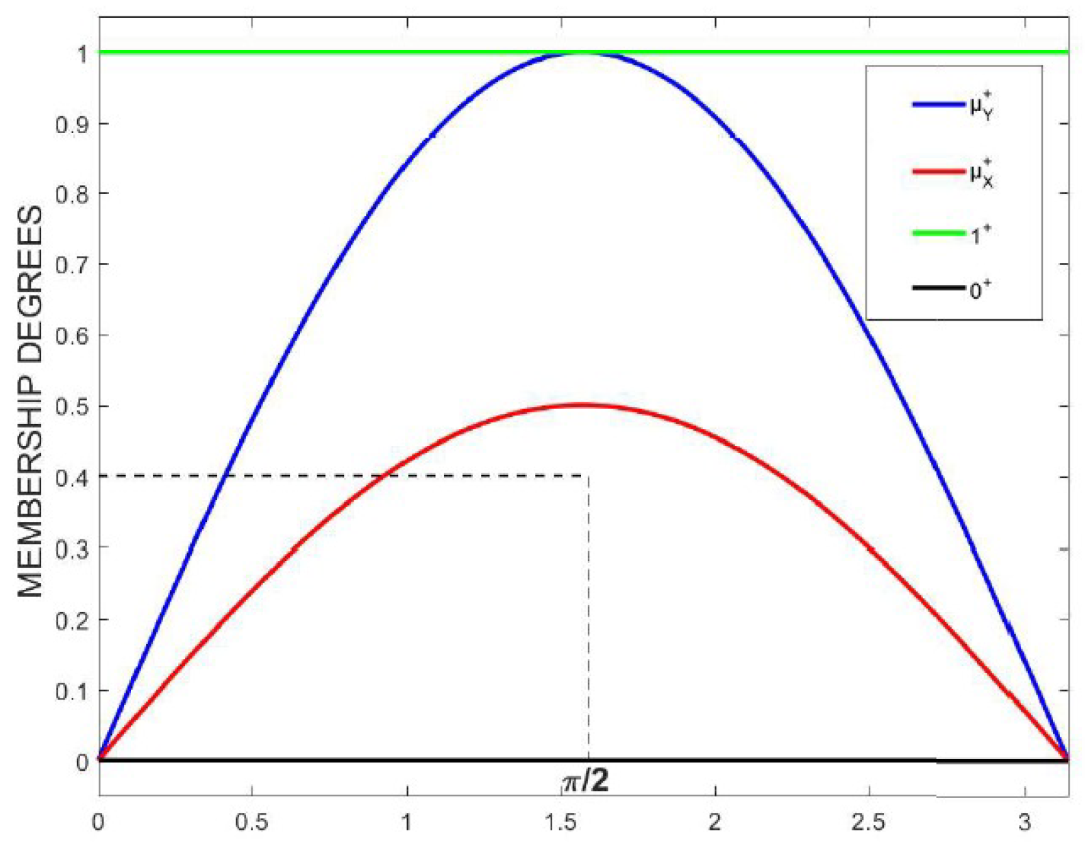
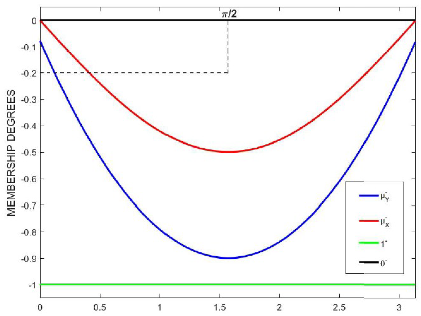
Let $U=[0,\pi ]$ and $\tau =\{\overline{0},\overline{1},A,B\}$. For each $u\in U$, $A=\{<u,{\mu }_A^{+}\left(u\right),{\mu }_A^{-}\left(u\right)>:u\in U\}$ and $B=\{<u,{\mu }_B^{+}\left(u\right),{\mu }_B^{-}\left(u\right)>:u\in U\}$ and membership functions given by

${\mu }_A^{+}\left(u\right)=\frac{sinu}{2}$, ${\mu }_A^{-}\left(u\right)=\frac{-sinu}{2}$ and ${\mu }_B^{+}\left(u\right)=cos(u-\frac{\pi }{2})$, ${\mu }_B^{-}\left(u\right)=\frac{1}{3}{(u-\frac{\pi }{2})}^2-0.9$

One can easily see that $A\subseteq B$ with the help of the graphs of membership functions given in Figure 2 and Figure 3.

It is clear that $\tau$ is a bipolar fuzzy supra topology on U. Therefore, for $u=\frac{\pi }{2},\alpha =0.4,\beta =-0.2$, we have

${\mu }_A^{+}\left(\frac{\pi }{2}\right)=0.5\ge 0.4$ , ${\mu }_A^{-}\left(\frac{\pi }{2}\right)=-0.5\le -0.2$ and ${\mu }_B^{+}\left(\frac{\pi }{2}\right)=1\ge 0.4$ , ${\mu }_B^{-}\left(\frac{\pi }{2}\right)=-0.9\le -0.2$ and $\overline{u}\in A\subseteq B$. So, we obtain $B\in N_{\tau }\left(\overline{u}\right)$.

With the following theorem, we characterize open sets by using neighborhoods.

Theorem 9.

Let $(U,\tau )$ be a bipolar fuzzy supra topological space and $A\in BPF\left(U\right)$. Then A is a bipolar fuzzy supra open set if and only if A is a bipolar fuzzy supra neighborhood of each of its bipolar fuzzy points.

Proof. 

Let A be a bipolar fuzzy supra open set and $\overline{u}\in A$, then by taking $B=A$, we obtain A is a bipolar fuzzy supra neighborhood of $\overline{u}$.

Conversely, suppose that A is a bipolar fuzzy supra neighborhood of each of its bipolar fuzzy points. Then, for every $\overline{u}\in A$, there exists a bipolar fuzzy supra open set $B_j$ such that $\overline{u}\in B_j\subseteq A$. Let $C={\bigcup }_{j\in J}{B}_j$. From the definition of bipolar fuzzy supra topology, C is a bipolar fuzzy supra open set. $C\subseteq A$ holds because $B_j\subseteq A$ for every $\overline{u}\in A$. Otherwise, every bipolar fuzzy point of A belongs to $B_j$, and therefore, they belong to C. Finally, we conclude that $A\subseteq C$ and $A=C$. This means that A is bipolar fuzzy supra open set. □

Now, we give the basic properties of the bipolar fuzzy supra neighborhood.

Theorem 10.

Let $(U,\tau )$ be a bipolar fuzzy supra topological space and $N_{\tau }\left(\overline{u}\right)$ be the neighborhood system of bipolar fuzzy point $\overline{u}$. Then we have the following:

N1. $N_{\tau }\left(\overline{u}\right)\ne \overline{0}$ for every $\overline{u}$.

N2. If $A\in N_{\tau }\left(\overline{u}\right)$, then $\overline{u}\in A$.

N3. If $A\subset B$ and $A\in N_{\tau }\left(\overline{u}\right)$, then $B\in N_{\tau }\left(\overline{u}\right)$.

N4. Let $A\in N_{\tau }\left(\overline{u}\right)$. Then there exists $B\in N_{\tau }\left(\overline{u}\right)$ such that $B\subset A$ and $B\in N_{\tau }\left(\overline{v}\right)$, $\forall \overline{v}\in B$.

Proof. 

N1. Let $\overline{u}\in \overline{1}$. Since $\overline{1}$ is a bipolar fuzzy supra open set, then $\overline{1}$ is a neighborhood of each of its bipolar fuzzy points. Therefore $N_{\tau }\left(\overline{u}\right)\ne \overline{0}$.

N2. Let $A\in N_{\tau }\left(\overline{u}\right)$, then there exists bipolar fuzzy supra open set C such that $\overline{u}\in C\subseteq A$, so $\overline{u}\in A$.

N3. Let $A\subset B$ and $A\in N_{\tau }\left(\overline{u}\right)$. Then there exists a bipolar fuzzy supra open set C such that $\overline{u}\in C\subseteq A$. Since $A\subset B$, then $\overline{u}\in C\subseteq B$ and $B\in N_{\tau }\left(\overline{u}\right)$.

N4. Let $A\in N_{\tau }\left(\overline{u}\right)$. Then there exists $C\in \tau$ such that $\overline{u}\in C\subseteq A$. Let $C:=B$ put a period. Thus we have $B\in N_{\tau }\left(\overline{u}\right)$. Now, let take $\overline{v}\in B$, then $B\in N_{\tau }\left(\overline{v}\right)$. Since $B\subseteq A$, it follows that $A\in N_{\tau }\left(\overline{v}\right)$. □

After proving the last two theorems, we should have a bipolar fuzzy supra topology determined by the neighborhood systems of a bipolar fuzzy point in a bipolar fuzzy supra topological space.

Theorem 11.

Let $N\left(\overline{u}\right)$ be a nonempty collection of bipolar fuzzy sets on U satisfying (N1)–(N4), for each bipolar fuzzy point $\overline{u}$. Then the family $\tau =\{A\in BPF\left(U\right):A\in N\left(\overline{v}\right),\forall \overline{v}\in A\}$ is a bipolar fuzzy supra topology on U such that $N\left(\overline{u}\right)$ is the family of all neighborhoods of $\overline{u}$ in $(U,\tau )$.

Proof. 

Let the subfamily $N\left(\overline{u}\right)\subset BPF\left(U\right)$ satisfy (N1)–(N4) for each $\overline{u}$ and let $\tau =\{A\in BPF\left(U\right):A\in N\left(\overline{v}\right),\forall \overline{v}\in A\}$. First, we need to see that $\tau$ is a bipolar fuzzy supra topology on U.

Since $\overline{0}$ contains no bipolar fuzzy points then $\overline{0}\in \tau$. We have $N\left(\overline{u}\right)\ne \overline{0}$. There must be a bipolar fuzzy supra neighborhood of each bipolar fuzzy points in U, which is $\overline{1}$, so $\overline{1}\in \tau$.

Let $\{A_j:j\in J\}\subseteq \tau$ and $A={\bigcup }_{j\in J}{A}_j$. If $\overline{u}\in A_j$ for any $j\in J$, then $\overline{u}\in {\bigcup }_{j\in J}{A}_j$. Since $A_j\in N\left(\overline{u}\right)$ and $A_j\subseteq A$, we have $A={\bigcup }_{j\in J}{A}_j\in N\left(\overline{u}\right)$. Therefore, $\tau$ is bipolar fuzzy supra topology on U.

For the remaining part of the proof, we need to show that $\tau$ is determined by a unique bipolar fuzzy supra neighborhood system, that is $N\left(\overline{u}\right)=N_{\tau }\left(\overline{u}\right)$. For each $A\in N_{\tau }\left(\overline{u}\right)$ there exists a $B\in \tau$ such that $\overline{u}\in B\subset A$. Since $\overline{u}\in B$ and $B\in \tau$, we have $B\in N\left(\overline{u}\right)$ and $A\in N\left(\overline{u}\right)$. Hence, $N_{\tau }\left(\overline{u}\right)\subset N\left(\overline{u}\right)$.

Conversely, let $A\in N\left(\overline{u}\right)$. Then, there exists a $B\in N\left(\overline{u}\right)$ such that $B\subseteq A$ and $B\in N\left(\overline{v}\right)$ for every $\overline{v}\in B$. It yields that $B\in \tau$. This implies that the bipolar fuzzy supra open set B is a bipolar fuzzy supra neighborhood of $\overline{u}$ so $B\in N_{\tau }\left(\overline{u}\right)$. Since $B\subseteq A$ we have $A\in N_{\tau }\left(\overline{u}\right)$. Then we conclude that $N\left(\overline{u}\right)\subset N_{\tau }\left(\overline{u}\right)$. Hence we obtain $N\left(\overline{u}\right)=N_{\tau }\left(\overline{u}\right)$. This completes the proof. □

Here, we present the characterization of continuous mapping by using bipolar fuzzy supra neighborhood.

Theorem 12.

Let $(U,\tau )$ and $(V,\sigma )$ be two bipolar fuzzy supra topological space, $\overline{u}\in BP{F}_P\left(U\right)$ and $f:(U,\tau )\to (V,\sigma )$ be a mapping. Then the following are equivalent:

1. f is a bipolar fuzzy supra continuous mapping.

2. $f^{-1}\left(B\right)\in N_{\tau }\left(\overline{u}\right)$ for each $B\in N_{\sigma }\left(f\left(\overline{u}\right)\right)$.

3. For each $\overline{u}\in BP{F}_P\left(U\right)$ and $B\in N_{\sigma }\left(f\left(\overline{u}\right)\right)$ there exists $A\in N_{\tau }\left(\overline{u}\right)$ such that $f\left(A\right)\subseteq B$.

Proof. 

($1\Rightarrow 2$) Suppose that $f:(U,\tau )\to (V,\sigma )$ is a bipolar fuzzy supra continuous mapping. If we take $B\in N_{\sigma }\left(f\left(\overline{u}\right)\right)$ then it is obvious that there exists a $C\in \sigma$ such that $f\left(\overline{u}\right)\in C\subset B$. Since f is bipolar fuzzy supra continuous we have $f^{-1}\left(C\right)\in \tau$ and therefore $\overline{u}\in f^{-1}\left(C\right)$ and $f^{-1}\left(C\right)\subset f^{-1}\left(B\right)$ is valid. Hence this implies that $f^{-1}\left(B\right)\in N_{\tau }\left(\overline{u}\right)$.

($2\Rightarrow 3$) Let $B\in N_{\sigma }\left(f\left(\overline{u}\right)\right)$. By hypothesis we obtain $f^{-1}\left(B\right)\in N_{\tau }\left(\overline{u}\right)$. Let choose $A=f^{-1}\left(B\right)$ one can easily see that $f\left(A\right)=f\left(f^{-1}\left(B\right)\right)\subseteq B$.

($3\Rightarrow 1$) To prove this statement we will show that $f^{-1}\left(B\right)\in \tau$ for each $B\in \sigma$. By taking $\overline{u}\in f^{-1}\left(B\right)$, we obtain $f\left(\overline{u}\right)\in B$ and thus $B\in N_{\sigma }\left(f\left(\overline{u}\right)\right)$ for each $B\in \sigma$. From the hypothesis there exists $A\in N_{\tau }\left(\overline{u}\right)$ such that $f\left(A\right)\subseteq B$. Then, by the properties of image and preimage, we have $A\subset f^{-1}\left(f\left(A\right)\right)\subset f^{-1}\left(B\right)$. Finally $A\subset f^{-1}\left(B\right)$ for each $A\in N_{\tau }\left(\overline{u}\right)$. Hence $f^{-1}\left(B\right)\in \tau$. □

4. Q-Neighborhood Structure of Bipolar Fuzzy Supra Topological Spaces

In 1980, Ming et al. [23] defined the concepts of quasi-coincident and Q-neighborhood. In this section, these two concepts are going to extend to bipolar fuzzy sets, and this allows us to study the Q-neighborhood structure of bipolar fuzzy supra topological spaces.

Definition 9.

1. Let $A,B\in BPF\left(U\right)$. Then we say that A is called quasi-coincident with B iff ${\mu }_A^{+}\left(u\right)+{\mu }_B^{+}\left(u\right)>1$ and ${\mu }_A^{-}\left(u\right)+{\mu }_B^{-}\left(u\right)<-1$ for $u\in U$. It is denoted by $AqB$.

2. Bipolar fuzzy point $\overline{u}\in BP{F}_P\left(U\right)$ is called quasi-coincident with A iff $\alpha +{\mu }_A^{+}\left(u\right)>1$ and $\beta +{\mu }_A^{-}\left(u\right)<-1$. It is denoted by $\overline{u}qA$ and opposite situation is denoted as $\overline{u}{q}^{c}A$.

In the following, we give an example of a quasi-coincident structure:

Example 5.

Let $U=\{u,v\}$$A=\{<u,0.9,-0.8>,<v,0.8,-0.7>\}$ and $B=\{<u,0.2,-0.3>,<v,0.3,-0.4>\}$. We obtain ${\mu }_A^{+}\left(z\right)+{\mu }_B^{+}\left(z\right)>1$ and ${\mu }_A^{-}\left(z\right)+{\mu }_B^{-}\left(z\right)<-1$ for each $z\in U$ and thus $AqB$.

Now, we offer some fundamental properties related to the concept of quasi-coincident.

Theorem 13.

Let $A,B\in BPF\left(U\right)$ and $\overline{u}\in BP{F}_P\left(U\right)$. Then, we have the statements below:

1. $\overline{u}{q}^c\overline{0}$.

2. $\overline{u}q\overline{1}$.

3. $AqB=BqA$.

4. $\overline{u}\in A\iff \overline{u}{q}^c{A}^c$.

5. $\overline{u}qA\iff \overline{u}\notin A^c$.

6. $A\subseteq B\iff A{q}^c{B}^c$.

7. $AqB\Rightarrow A\cap B\ne \overline{0}$.

8. $A{q}^c{A}^c$.

9. $AqB\iff Thereexists\overline{u}\in A$ such that $\overline{u}qB$.

10. $\overline{u}\in A^c\iff \overline{u}{q}^{c}A$.

11. Let $A\subseteq B$. If $\overline{u}qA$, then $\overline{u}qB$.

Proof. 

1, 2, and 3 are clear from the definition.

4.

$\overline{u}\in A$	⇔	${\mu }_A^{+}\left(u\right)\ge \alpha and{\mu }_A^{-}\left(u\right)\le \beta$
	⇔	${\mu }_{{\left(A^c\right)}^c}^{+}\left(u\right)\nless \alpha and{\mu }_{{\left(A^c\right)}^c}^{-}\left(u\right)\ngtr \beta$
	⇔	$\overline{u}{q}^c{A}^c$.

5.

$\overline{u}qA$	⇔	$\alpha +{\mu }_A^{+}\left(u\right)>1and\beta +{\mu }_A^{-}\left(u\right)<-1$
	⇔	$\alpha >1-{\mu }_A^{+}\left(u\right)and\beta <-1-{\mu }_A^{-}\left(u\right)$
	⇔	$\overline{u}\notin A^c$.

6. Suppose that $A\subseteq B$. Then ${\mu }_A^{+}\left(u\right)\le {\mu }_B^{+}\left(u\right)$ and ${\mu }_A^{-}\left(u\right)\ge {\mu }_B^{-}\left(u\right)$ for each $u\in U$. We can write the following inequality

${\mu }_A^{+}\left(u\right)+{\mu }_{B^c}^{+}\left(u\right)$	=	${\mu }_A^{+}\left(u\right)+1-{\mu }_B^{+}\left(u\right)$
	≤	${\mu }_B^{+}\left(u\right)+1-{\mu }_B^{-}\left(u\right)$
	=	1

and therefore ${\mu }_A^{+}\left(u\right)+{\mu }_{B^c}^{+}\left(u\right)\le 1$.

For the negative part, we have

${\mu }_A^{-}\left(u\right)+{\mu }_{B^c}^{-}\left(u\right)$	=	${\mu }_A^{-}\left(u\right)-1-{\mu }_B^{-}\left(u\right)$
	≥	${\mu }_B^{-}\left(u\right)-1-{\mu }_B^{-}\left(u\right)$
	=	$-1$

By combining the two inequalities, we obtain $A{q}^c{B}^c$. Converse of the theorem can be shown by the same token.

7.

$AqB$	⇒	${\mu }_A^{+}\left(u\right)+{\mu }_B^{+}\left(u\right)>1and{\mu }_A^{-}\left(u\right)+{\mu }_B^{-}\left(u\right)<-1$
	⇒	${\mu }_A^{+}\left(u\right),{\mu }_B^{+}\left(u\right)\ne 0and{\mu }_A^{-}\left(u\right),{\mu }_B^{-}\left(u\right)\ne 0$
	⇒	${\mu }_A^{+}\left(u\right)\wedge {\mu }_B^{+}\left(u\right)\ne 0and{\mu }_A^{-}\left(u\right)\vee {\mu }_B^{-}\left(u\right)\ne 0$
	⇒	$A\cap B\ne \overline{0}$.

8. ${\mu }_A^{+}\left(u\right)+{\mu }_{A^c}^{+}\left(u\right)={\mu }_A^{+}\left(u\right)+1-{\mu }_A^{+}\left(u\right)=1$ and ${\mu }_A^{-}\left(u\right)+{\mu }_{A^c}^{-}\left(u\right)={\mu }_A^{+}\left(u\right)-1-{\mu }_A^{-}\left(u\right)=-1$. Thus, we obtain $A{q}^c{A}^c$.

9. Let $AqB$ and $\overline{u}\in A$. Hence, we obtain ${\mu }_A^{+}\left(u\right)+{\mu }_B^{+}\left(u\right)>1$ and ${\mu }_A^{-}\left(u\right)+{\mu }_B^{-}\left(u\right)<-1$. By taking $\alpha ={\mu }_A^{+}\left(u\right)$ and $\beta ={\mu }_A^{-}\left(u\right)$ we have what we desired. Thus, $\overline{u}qB$.

Conversely, suppose that $\overline{u}\in A$ and $\overline{u}qB$. Then, $\alpha \le {\mu }_A^{+}\left(u\right)$ and $\beta \ge {\mu }_A^{-}\left(u\right)$. From here, ${\mu }_A^{+}\left(u\right)+{\mu }_B^{+}\left(u\right)\ge \alpha +{\mu }_B^{+}\left(u\right)>1$ and ${\mu }_A^{-}\left(u\right)+{\mu }_B^{-}\left(u\right)\le \beta +{\mu }_B^{-}\left(u\right)<-1$ and these inequalities give the result which is $AqB$.

10.

$\overline{u}\in A^c$	⇔	$\alpha \le {\mu }_{A^c}^{+}\left(u\right)and\beta \ge +{\mu }_{A^c}^{-}\left(u\right)$
	⇔	$\alpha \le 1-{\mu }_A^{+}\left(u\right)and\beta \ge -1-{\mu }_A^{-}\left(u\right)$
	⇔	$\alpha +{\mu }_A^{+}\left(u\right)\le 1and\beta +{\mu }_A^{-}\left(u\right)\ge -1$
	⇔	$\overline{u}{q}^{c}A$.

11. Let $A\subseteq B$ and $\overline{u}qA$ be given. Then it follows that $\alpha +{\mu }_A^{+}\left(u\right)>1$ and $\beta +{\mu }_A^{-}\left(u\right)<-1$. Since $A\subseteq B$, we write $\alpha +{\mu }_B^{+}\left(u\right)\ge \alpha +{\mu }_A^{+}\left(u\right)>1$ and $\beta +{\mu }_B^{-}\left(u\right)\le \beta +{\mu }_A^{-}\left(u\right)<-1$. Finally, we conclude that $\overline{u}qB$. □

Proposition 2.

Let $\left(A_j\right)\subset BPF\left(U\right)$ and $\overline{u}\in BP{F}_P\left(U\right)$. Then the following are hold:

1. $\overline{u}q\left({\bigcap }_{j\in J}{A}_j\right)\iff \overline{u}q\left(A_j\right),\forall j\in J$.

2. $\overline{u}q\left({\bigcup }_{j\in J}{A}_j\right)\iff \overline{u}q\left(A_j\right),\exists j\in J$.

Proof. 

1. Let $\overline{u}q\left({\bigcap }_{j\in J}{A}_j\right)$. Then we have $\alpha +{\wedge }_{j\in J}{\mu }_{A_j}^{+}\left(u\right)>1$ and $\beta +{\vee }_{j\in J}{\mu }_{A_j}^{-}\left(u\right)<-1$. Since ${\mu }_{A_j}^{+}\left(u\right)\ge {\wedge }_{j\in J}{\mu }_{A_j}^{+}\left(u\right)$ and ${\mu }_{A_j}^{-}\left(u\right)\le {\vee }_{j\in J}{\mu }_{A_j}^{-}\left(u\right),j\in J$, we obtain $\alpha +{\mu }_{A_j}^{+}\left(u\right)\ge \alpha +{\wedge }_{j\in J}{\mu }_{A_j}^{+}\left(u\right)>1$ and $\beta +{\mu }_{A_j}^{-}\left(u\right)\le \beta +{\vee }_{j\in J}{\mu }_{A_j}^{-}\left(u\right)<-1$. Hence, $\overline{u}q\left(A_j\right),\forall j\in J$.

Conversely, let $\overline{u}q\left(A_j\right),\forall j\in J$. Then, $\alpha +{\mu }_{A_j}^{+}\left(u\right)>1$ and $\beta +{\mu }_{A_j}^{-}\left(u\right)<-1$.

⇒$\alpha +{\bigwedge }_{j\in J}{\mu }_{A_j}^{+}\left(u\right)>1$ and $\beta +{\bigvee }_{j\in J}{\mu }_{A_j}^{-}\left(u\right)<-1$.

⇒$\overline{u}q\left({\bigcap }_{j\in J}{A}_j\right)$

2.

$\overline{u}q\left({\bigcup }_{j\in J}{A}_j\right)$	⇔	$\overline{u}\notin {\left({\bigcup }_{j\in J}{A}_j\right)}^c$	□
	⇔	$\overline{u}\notin {\bigcap }_{j\in J}{\left(A_j\right)}^c$
	⇔	$\overline{u}\notin {\left(A_j\right)}^c,\exists j\in J$
	⇔	$\overline{u}q{A}_j,\exists j\in J$.

Definition 10.

Let τ be a bipolar fuzzy supra topology on U, $\overline{u}\in BP{F}_P\left(U\right)$ and $A\in BPF\left(U\right)$. A is called Q-neighborhood of $\overline{u}$ if there exists $B\in \tau$ such that $\overline{u}qB$ and $B\subseteq A$. The family of all Q-neighborhood of the $\overline{u}$ is denoted by $Q_{\tau }\left(\overline{u}\right)$.

Example 6.

Let $U=\{u,v\}$ and $\tau =\{\overline{0},\overline{1},A\}$, where $A=\{<u,1,-0.6>,<v,0.7,-1>\}$. Take $\overline{u}=\{<x,0.4,-0.5>\}$. Since $\overline{u}qA$ and $A\subseteq \overline{1}$ it follows that $\overline{1}\in Q_{\tau }\left(\overline{u}\right)$.

In the next example, we see that a Q-neighborhood of bipolar fuzzy point generally may not contain the point itself.

Example 7.

Let take a bipolar fuzzy supra topology as $\tau =\{\overline{0},\overline{1},A,B\}$, where $A=\{<u,0.7,-0.3>,<v,0.5,-0.4>\}$, $B=\{<u,0.6,-0.1>,<v,0.4,-0.1>\}$. Now if we take $\overline{u}=\{<u,0.5,-0.95>\}$, we thus have $\overline{u}qB$ and $B\subseteq A$, therefore $A\in Q_{\tau }\left(\overline{u}\right)$. Considering the given data we obtain $\alpha =0.5<0.7={\mu }_A^{+}\left(u\right)$ and $\beta =-0.95\ngtr -0.3={\mu }_A^{-}\left(u\right)$, so $\overline{u}\notin A$.

In the following theorem, we study the basic properties of the bipolar fuzzy supra Q-neighborhood.

Theorem 14.

Let $(U,\tau )$ be a bipolar fuzzy supra topological space and $Q_{\tau }\left(\overline{u}\right)$ be the family of all Q neighborhoods of $\overline{u}$. Then we have the following:

Q1. $\overline{1}\in Q_{\tau }\left(\overline{u}\right)$ and if $A\in Q_{\tau }\left(\overline{u}\right)$, then $\overline{u}qA$.

Q2. If $B\subseteq A$ and $B\in Q_{\tau }\left(\overline{u}\right)$, then $A\in Q_{\tau }\left(\overline{u}\right)$.

Q3. Let $A\in Q_{\tau }\left(\overline{u}\right)$. Then there exists $B\in Q_{\tau }\left(\overline{u}\right)$ such that $B\subseteq A$ and $B\in Q_{\tau }\left(\overline{v}\right)$, $\forall \overline{v}qB$.

Proof. 

Q1. To see $\overline{1}\in Q_{\tau }\left(\overline{u}\right)$ we need to show that there exists $B\in \tau$ satisfying $\overline{u}qB$ and $B\subseteq \overline{1}$ for any $\overline{u}\in BP{F}_P\left(U\right)$. If we choose $B:=\overline{1}$, then we are done. Now, let $A\in Q_{\tau }\left(\overline{u}\right)$. Then there exists $B\in \tau$ such that $\overline{u}qB$ and $B\subseteq A$ holds. From here, $\alpha +{\mu }_A^{+}\left(u\right)\ge \alpha +{\mu }_B^{+}\left(u\right)>1$ and $\beta +{\mu }_A^{-}\left(u\right)\le \beta +{\mu }_B^{-}\left(u\right)<-1$, consequently $\overline{u}qA$.

Q2. Let $B\subseteq A$ and $B\in Q_{\tau }\left(\overline{u}\right)$. Then there exists $C\in \tau$ such that $\overline{u}qC$ and $C\subseteq B$. Since $B\subseteq A$, $\overline{u}qC\subseteq A$ and $A\in Q_{\tau }\left(\overline{u}\right)$.

Q3. Let $A\in Q_{\tau }\left(\overline{u}\right)$. Then there exists $B\in \tau$ such that $\overline{u}qB$ and $B\subseteq A$. By choosing $B:=A$ we obtain $B\in Q_{\tau }\left(\overline{u}\right)$. Moreover, since $B\in \tau$, then B is a Q neighborhood of any bipolar fuzzy points that are contained in it. So $\overline{v}qB$ and $B\in Q_{\tau }\left(\overline{v}\right)$. □

Theorem 15.

Let $Q\left(\overline{u}\right)$ be nonempty collection of bipolar fuzzy sets on U satisfying (Q1)–(Q3) for each bipolar fuzzy point $\overline{u}$. Then the family $\tau =\{A\in BPF\left(U\right):A\in Q\left(\overline{v}\right),\forall \overline{v}qA\}\cup \left\{\overline{0}\right\}$ is a bipolar fuzzy supra topology on U such that $Q\left(\overline{u}\right)$ is the family of all Q-neighborhoods of $\overline{u}$ in $(U,\tau )$.

Proof. 

Let the subfamily $Q\left(\overline{u}\right)\subset BPF\left(U\right)$ satisfies the conditions (Q1)–(Q3) for each $\overline{u}$ and let $\tau =\{A\in BPF\left(U\right):A\in Q\left(\overline{v}\right),\forall \overline{v}qA\}\cup \left\{\overline{0}\right\}$. Firstly, we need to show that $\tau$ is a bipolar fuzzy supra topology. From the definition of $\tau$, we have $\overline{0}\in \tau$ and $\overline{1}\in \tau$ by Theorem 14. Now let $\{A_j:j\in J\}\subseteq \tau$, then $A_j\in \tau ,\forall j\in J$, we have $A_j\in Q\left(\overline{u}\right)$ and $\overline{x}q{A}_j$. Hence, ${\bigcup }_{j\in J}{A}_j\in Q\left(\overline{u}\right)$. Furthermore, for every $j\in J$ and $u\in U$, we have $1<\alpha +{\mu }_{A_j}^{+}\left(u\right)\le \alpha +{\vee }_{j\in J}{\mu }_{A_j}^{+}\left(u\right)$ and $-1>\beta +{\mu }_{A_j}^{-}\left(u\right)\ge \beta +{\wedge }_{j\in J}{\mu }_{A_j}^{-}\left(u\right)$, then it follows that $\overline{u}q\left({\bigcup }_{j\in J}{A}_j\right)$. Finally we conclude that ${\bigcup }_{j\in J}{A}_j\in \tau$.

Now we show that $Q\left(\overline{u}\right)=Q_{\tau }\left(\overline{u}\right)$. Suppose that $A\in Q_{\tau }\left(\overline{u}\right)$. Then we have $B\in \tau$ such that $\overline{u}qB$ and $B\subseteq A$. Then $B\in Q\left(\overline{u}\right)$ and thus $A\in Q\left(\overline{u}\right)$. So, we obtain $Q_{\tau }\left(\overline{u}\right)\subseteq Q\left(\overline{u}\right)$. For the converse , take $A\in Q\left(\overline{u}\right)$. By the Theorem 14 there exists $B\in Q\left(\overline{u}\right)$ such that for every $\overline{v}qB$ we have $B\subseteq A$ and $B\in Q\left(\overline{v}\right)$. Moreover, $B\in Q\left(\overline{u}\right)$, then $\overline{u}qB$ and $B\in \tau$. Since $B\subseteq A$, $A\in Q_{\tau }\left(\overline{u}\right)$. Hence, we have $Q\left(\overline{u}\right)\subseteq Q_{\tau }\left(\overline{u}\right)$. □

5. Bipolar Fuzzy Supra Topology in Data Mining

In the last section, we give an application of bipolar fuzzy set in methodical approach for medical diagnosis problems. The methodical technique to select the appropriate qualities and alternatives in the decision-making problem is given in the following stages. Here, we employ the method in [35].

Step 1: Problem Area Selection:

Examine multi-criteria decision-making problems involving m attributes $A_1,A_2,\dots ,A_m$ and n alternatives $C_1,C_2,\dots ,C_n$ and p attributes $D_1,D_2,\dots ,D_p$, ($n\le p$).

All attributes $a_{ij}$ and $d_{ki}$ are bipolar fuzzy numbers for $i=\overline{1,m}$, $j=\overline{1,n}$, $k=\overline{1,p}$.

Step 2: Form bipolar fuzzy supra topologies for ($C_j$) and ($D_k$):

(i) ${\tau }_j=E\cup F$, where $E=\{\overline{0},\overline{1},a_{1j},a_{2j},\dots ,a_{mj}\}$ and $F=\{a_{1j}\cup a_{2j},a_{1j}\cup a_{3j},\dots ,a_{m-1j}\cup a_{mj}\}$.

(ii) ${\sigma }_k=G\cup H$, where $G=\{\overline{0},\overline{1},d_{k1},d_{k2},\dots ,d_{km}\}$ and $H=\{d_{k1}\cup d_{k2},d_{k1}\cup d_{k3},\dots ,d_{km-1}\cup d_{km}\}$.

Step 3: Find Bipolar fuzzy score functions:

Bipolar fuzzy score functions (BFSF) of $E,F,G,H,C_j$ and $D_k$ are defined as follows:

(i) $BFSF\left(E\right)=\frac{1}{2(m+2)}\left({\sum }_{i=1}^{m+2}\frac{1+{\mu }_i^{+}+{\mu }_i^{-}}{2}\right)$ and $BFSF\left(F\right)=\frac{1}{2t}\left({\sum }_{i=1}^t\frac{1+{\mu }_i^{+}+{\mu }_i^{-}}{2}\right)$, where t is the number of elements of F.

${\displaystyle BFSF\left(C_j\right)=\left\{\begin{array}{cc}BFSF\left(E\right),\hfill & \mathrm{if}BFSF\left(F\right)=0;\hfill \\ \frac{BFSF\left(E\right)+BFSF\left(F\right)}{2},\hfill & \mathrm{otherwise}\hfill \end{array}\right.}$, for $j=\overline{1,n}$.

(ii) $BFSF\left(G\right)=\frac{1}{2(m+2)}\left({\sum }_{i=1}^{m+2}\frac{1+{\mu }_i^{+}+{\mu }_i^{-}}{2}\right)$ and $BFSF\left(H\right)=\frac{1}{2s}\left({\sum }_{i=1}^s\frac{1+{\mu }_i^{+}+{\mu }_i^{-}}{2}\right)$, where s is the number of elements of H.

${\displaystyle BFSF\left(D_k\right)=\left\{\begin{array}{cc}BFSF\left(G\right),\hfill & \mathrm{if}BFSF\left(H\right)=0;\hfill \\ \frac{BFSF\left(G\right)+BFSF\left(H\right)}{2},\hfill & \mathrm{otherwise}\hfill \end{array}\right.}$, for $k=\overline{1,p}$.

Step 4: Final Decision:

Determine bipolar fuzzy score values for the alternatives $C_1\le C_2\le C_3\le \dots \le C_n$ and the attributes $D_1\le D_2\le \dots \le D_p$. Select the attribute $D_p$ for the alternative $C_1$, $D_{p-1}$ for alternative $C_2$ and $D_{p-2}$ for alternative $C_3$, etc. If $n<p$, then ignore $D_k$, where $k=\overline{1,n-p}$.

Case Study

Dealing with uncertainty is inherent in medical diagnosis problems, and the introduction of bipolar fuzzy sets offers a valuable perspective. In this section, we present an illustrative medical diagnosis problem to demonstrate the applicability of the mentioned approach.

Step 1: Problem Area Selection:

Suppose that $P=\{P_1,P_2,P_3,P_4\}$ be the set of patients,

$S=\{Temperature,Cough,BloodPlates,JointPain,Insulin\}$ be the set symptoms and

$R=\{Tuberculosis,Diabetes,Chikungunya,SwineFlu,Dengue\}$ be the set of diseases corresponding to the symptoms S.

We need to find the patient and to find the disease of the patient.

Patient−Symptom Relation
Symptoms	Patients
	P1	P2	P3	P4
Temperature	(0.8, −0.1)	(0.4, −0.5)	(0.5, −0.6)	(0.9, −0.4)
Cough	(0.3, −0.5)	(0.4, −0.8)	(0.6, −0.4)	(0.9, −0.2)
Blood Plates	(0.1, −0.3)	(0.7, −0.2)	(0.3, −0.9)	(0.4, −0.7)
Joint pain	(0.4, −0.5)	(0.6, −0.5)	(0.6, −0.3)	(0.5, −0.7)
Insulin	(0.8, −0.2)	(0.7, −0.3)	(0.3, −0.6)	(0.2, −0.5)

Symptom-Disease Relation
Diagnosis	Symptoms
	Temperature	Cough	Blood Plates	Joint pain	Insulin
Tuberculosis	(0.6, −0.1)	(0.9, −0.1)	(0, −0.8)	(0, −0.8)	(0, −0.9)
Diabetes	(0.1, −0.8)	(0.1, −0.8)	(0.2, −0.1)	(0.2, −0.5)	(0.9, −0.1)
Chikungunya	(0.9, −0.1)	(0, −0.8)	(0.7, −0.1)	(0.9, −0.1)	(0.2, −0.8)
Swine Flue	(0.2, −0.3)	(0.1, −0.3)	(0.2, −0.1)	(0.1, −0.5)	(0.2, −0.1)
Dengeu	(0.9, −0.1)	(0.2, −0.4)	(0.2, −0.4)	(0.3, −0.7)	(0.2, −0.7)

Step 2: Form bipolar fuzzy supra topologies for ($C_j$) and ($D_k$):

For ($C_j$);

(i) ${\tau }_1=E\cup F$, where

$E=\{\overline{0},\overline{1},a_{11},a_{21},a_{31},a_{41},a_{51}\}=\{\overline{0},\overline{1},(0.8,-0.1),(0.3,-0.5),(0.8,-0.2),(0.4,-0.5),(0.1,-0.3)\}$ and $F=\{a_{11}\cup a_{21},a_{11}\cup a_{31},a_{11}\cup a_{41},a_{11}\cup a_{51},a_{21}\cup a_{31},a_{21}\cup a_{41},a_{21}\cup a_{51},a_{31}\cup a_{41},a_{31}\cup a_{51},a_{41}\cup a_{51}\}$.

We omit some bipolar fuzzy sets of F which are in E and we obtain $F=\left\{\right(0.8,-0.3),(0.3,-0.5\left)\right\}$.

(ii) ${\tau }_2=E\cup F$, where

$E=\{\overline{0},\overline{1},a_{12},a_{22},a_{32},a_{42},a_{52}\}=\{\overline{0},\overline{1},(0.4,-0.5),(0.4,-0.8),(0.7,-0.2),(0.6,-0.5),(0.7,-0.3)\}$ and $F=\{a_{12}\cup a_{22},a_{12}\cup a_{32},a_{12}\cup a_{42},a_{12}\cup a_{52},a_{22}\cup a_{32},a_{22}\cup a_{42},a_{22}\cup a_{52},a_{32}\cup a_{42},a_{32}\cup a_{52},a_{42}\cup a_{52}\}$ = $\left\{\right(0.7,-0.8),(0.7,-0.5),(0.6,-0.8\left)\right\}$.

(iii) ${\tau }_3=E\cup F$, where

$E=\{\overline{0},\overline{1},a_{13},a_{23},a_{33},a_{43},a_{53}\}=\{\overline{0},\overline{1},(0.5,-0.6),(0.6,-0.4),(0.3,-0.9),(0.6,-0.3),(0.3,-0.6)\}$ and $F=\{a_{13}\cup a_{23},a_{13}\cup a_{33},a_{13}\cup a_{43},a_{13}\cup a_{53},a_{23}\cup a_{33},a_{23}\cup a_{43},a_{23}\cup a_{53},a_{33}\cup a_{43},a_{33}\cup a_{53},a_{43}\cup a_{53}\}$ = $\left\{\right(0.6,-0.9),(0.6,-0.6),(0.5,-0.9\left)\right\}$.

(iv) ${\tau }_4=E\cup F$, where

$E=\{\overline{0},\overline{1},a_{14},a_{24},a_{34},a_{44},a_{54}\}=\{\overline{0},\overline{1},(0.9,-0.4),(0.9,-0.2),(0.4,-0.7),(0.5,-0.7),(0.2,-0.5)\}$ and $F=\{a_{14}\cup a_{24},a_{14}\cup a_{34},a_{14}\cup a_{44},a_{14}\cup a_{54},a_{24}\cup a_{34},a_{24}\cup a_{44},a_{24}\cup a_{54},a_{34}\cup a_{44},a_{34}\cup a_{54},a_{44}\cup a_{54}\}$ = $\left\{\right(0.9,-0.5),(0.9,-0.7\left)\right\}$.

For ($D_k$);

(i) ${\sigma }_1=G\cup H$, where

$G=\{\overline{0},\overline{1},d_{11},d_{12},d_{13},d_{14},d_{15}\}=\{\overline{0},\overline{1},(0.6,-0.1),(0.9,-0.1),(0,-0.8),(0,-0.8),(0,-0.9)\}$ and $H=\{d_{11}\cup d_{12},d_{11}\cup d_{13},d_{11}\cup d_{14},d_{11}\cup d_{15},d_{12}\cup d_{13},d_{12}\cup d_{14},d_{12}\cup d_{15},d_{13}\cup d_{14},d_{13}\cup d_{15},d_{14}\cup d_{15}\}$.

We omit some bipolar fuzzy sets of H which are in G and we obtain

$H=\left\{\right(0.6,-0.8),(0.6,-0.9),(0.9,-0.8),(0.9,-0.9\left)\right\}$.

(ii) ${\sigma }_2=G\cup H$, where

$G=\{\overline{0},\overline{1},d_{21},d_{22},d_{23},d_{24},d_{25}\}=\{\overline{0},\overline{1},(0.1,-0.8),(0.1,-0.8),(0.2,-0.1),(0.2,-0.5),(0.9,-0.1)\}$ and $H=\{d_{21}\cup d_{22},d_{21}\cup d_{23},d_{21}\cup d_{24},d_{21}\cup d_{25},d_{22}\cup d_{23},d_{22}\cup d_{24},d_{22}\cup d_{25},d_{23}\cup d_{24},d_{23}\cup d_{25},d_{24}\cup d_{25}\}$= $\left\{\right(0.2,-0.8),(0.9,-0.8),(0.9,-0.5\left)\right\}$.

(iii) ${\sigma }_3=G\cup H$, where

$G=\{\overline{0},\overline{1},d_{31},d_{32},d_{33},d_{34},d_{35}\}=\{\overline{0},\overline{1},(0.9,-0.1),(0,-0.8),(0.7,-0.1),(0.9,-0.1),(0.2,-0.8)\}$ and $H=\{d_{31}\cup d_{32},d_{31}\cup d_{33},d_{31}\cup d_{34},d_{31}\cup d_{35},d_{32}\cup d_{33},d_{32}\cup d_{34},d_{32}\cup d_{35},d_{33}\cup d_{34},d_{33}\cup d_{35},d_{34}\cup d_{35}\}$ = $\left\{\right(0.9,-0.8),(0.7,-0.8\left)\right\}$.

(iv) ${\sigma }_4=G\cup H$, where

$G=\{\overline{0},\overline{1},d_{41},d_{42},d_{43},d_{44},d_{45}\}=\{\overline{0},\overline{1},(0.2,-0.3),(0.1,-0.3),(0.2,-0.1),(0.1,-0.5),(0.2,-0.1)\}$ and $H=\{d_{41}\cup d_{42},d_{41}\cup d_{43},d_{41}\cup d_{44},d_{41}\cup d_{45},d_{42}\cup d_{43},d_{42}\cup d_{44},d_{42}\cup d_{45},d_{43}\cup d_{44},d_{43}\cup d_{45},d_{44}\cup d_{45}\}$ = $\left\{\right(0.2,-0.5\left)\right\}$.

(v) ${\sigma }_5=G\cup H$, where

$G=\{\overline{0},\overline{1},d_{51},d_{52},d_{53},d_{54},d_{55}\}=\{\overline{0},\overline{1},(0.9,-0.1),(0.2,-0.4),(0.2,-0.4),(0.3,-0.7),(0.2,-0.7)\}$ and $H=\{d_{51}\cup d_{52},d_{51}\cup d_{53},d_{51}\cup d_{54},d_{51}\cup d_{55},d_{52}\cup d_{53},d_{52}\cup d_{54},d_{52}\cup d_{55},d_{53}\cup d_{54},d_{53}\cup d_{55},d_{54}\cup d_{55}\}$ = $\left\{\right(0.9,-0.4),(0.9,-0.7\left)\right\}$.

Step 3: Find Bipolar fuzzy score functions:

For $\left(C_j\right)$,

(i) $BFSF\left(E\right)=0.2786$ and $BFSF\left(F\right)=0.2875$, where $t=2$. $BFSF\left(C_1\right)=0.2831$.

(ii) $BFSF\left(E\right)=0.2679$ and $BFSF\left(F\right)=0.2417$, where $t=3$. $BFSF\left(C_2\right)=0.2548$.

(iii) $BFSF\left(E\right)=0.2321$ and $BFSF\left(F\right)=0.1917$, where $t=3$. $BFSF\left(C_3\right)=0.2119$.

(iv) $BFSF\left(E\right)=0.2643$ and $BFSF\left(F\right)=0.3250$, where $t=2$. $BFSF\left(C_4\right)=0.2947$.

For $\left(D_k\right)$,

(i) $BFSF\left(G\right)=0.22071$ and $BFSF\left(H\right)=0.2250$, where $s=4$. $BFSF\left(D_1\right)=0.2161$.

(ii) $BFSF\left(G\right)=0.2857$ and $BFSF\left(F\right)=0.2417$, where $s=3$. $BFSF\left(D_2\right)=0.2637$.

(iii) $BFSF\left(G\right)=0.2786$ and $BFSF\left(H\right)=0.2500$, where $s=2$. $BFSF\left(D_3\right)=0.2643$.

(iv) $BFSF\left(G\right)=0.2321$ and $BFSF\left(H\right)=0.175$, where $s=1$. $BFSF\left(D_4\right)=0.2036$.

(v) $BFSF\left(G\right)=0.2321$ and $BFSF\left(H\right)=0.3375$, where $s=2$. $BFSF\left(D_6\right)=0.2848$.

Step 4: Final Decision:

By organizing bipolar fuzzy score values for the alternatives $C_1,C_2,C_3,C_4$ and the attributes $D_1,D_2,D_3,D_4,D_5$ in ascending order, we obtain the following order $C_3\le C_2\le C_1\le C_4$ and $D_4\le D_1\le D_2\le D_3\le D_5$. Thus the patient $P_3$ suffers from dengue, the patient $P_2$ suffers from chikungunya, the patient $P_1$ suffers from diabetes, the patient $P_4$ suffers form tuberculosis.

6. Conclusions

With this study, we focus on the notions of bipolar fuzzy neighborhoods and the Q-neighborhood of a bipolar fuzzy point in bipolar fuzzy supra topological spaces and also investigate the necessary conditions for a family of bipolar fuzzy sets to generate a bipolar fuzzy supra topology. Finally, we present a method for data analysis under a bipolar fuzzy supra topological environment as a real-life application. These concepts play useful roles in further research. Generalizations of fuzzy sets have been successfully used in various fields such as economics, environmental science, engineering, and especially in decision-making problems. A bipolar fuzzy set is a new kind of fuzzy set dealing with positive and negative aspects. In recent years, some of the other fuzzy set generalizations have been combined with a bipolar fuzzy set; for instance, bipolar intuitionistic fuzzy sets [36], bipolar picture fuzzy set [37]. With the help of these novel fuzzy sets, similar applications may be studied by defining the supra topology, and also this theory can be developed in other research areas of general topology.

References

- Zadeh, L.A. Fuzzy sets. Inf. Control 1965, 8, 338–353. [Google Scholar] [CrossRef]
- Atanassov, K.T. Intuitionistic fuzzy sets. Fuzzy Sets Syst. 1986, 20, 87–96. [Google Scholar] [CrossRef]
- Yager, R.R. Pythagorean fuzzy subsets. In Proceedings of the IFSA World Congress and NAFIPS Annual Meeting (IFSA/NAFIPS), Edmonton, AL, Canada, 24–28 June 2013; pp. 57–61. [Google Scholar]
- Smarandache, F. A Unifying Field in Logics. Neutrosophy/Neutrosophic Probability, Set and Logic; American Research Press: Rehoboth, DE, USA, 1998. [Google Scholar]
- Cuong, B.C.; Kreinovich, V. Picture fuzzy sets-a new concept for computational intelligence problems. In Proceedings of the 2013 World Congress on Information and Communication Technologies (WICT 2013), Hanoi, Vietnam, 15–18 December 2013; pp. 1–6. [Google Scholar]
- Gündogdu, F.K.; Kahraman, C. Spherical fuzzy sets and spherical fuzzy TOPSIS method. J. Intell. Fuzzy Syst. 2019, 36, 337–352. [Google Scholar] [CrossRef]
- Zhang, W.-R. Bipolar fuzzy sets and relations: A computational framework for cognitive modeling and multiagent decision analysis. In Proceedings of the NAFIPS/IFIS/NASA’94, Proceedings of the First International Joint Conference of The North American Fuzzy Information Processing Society Biannual Conference, San Antonio, TX, USA, 18–21 December 1994; pp. 305–309. [Google Scholar]
- Lee, K.M. Bipolar-valued fuzzy sets and their operaitons. In Proceedings of the International Conference on Intelligent Technologies, Bangkok, Thailand, 13–15 December 2000; pp. 307–312. [Google Scholar]
- Zhang, W.-R. The road from fuzzy sets to definable causality and bipolar quantum intelligence—To the memory of Lotfi A. Zadeh. J. Intell. Fuzzy Syst. 2019, 36, 3019–3032. [Google Scholar] [CrossRef]
- Zhang, W.-R. Science vs. Sophistry—A historical debate on bipolar fuzzy sets and equilibrium-based mathematics for AI and QI. J. Intell. Fuzzy Syst. 2021, 41, 6781–6799. [Google Scholar] [CrossRef]
- Lee, K.M. Bipolar fuzzy subalgebras and bipolar fuzzy ideals of BCK/BCI-algebras. Bull. Malays. Math. Sci. Soc. 2009, 32, 361–373. [Google Scholar]
- Abdullah, S.; Aslam, M.; Ullah, K. Bipolar fuzzy soft sets and its applications in decision making problem. J. Intell. Fuzzy Syst. 2014, 27, 729–742. [Google Scholar] [CrossRef]
- Kim, J.H.; Samanta, S.K.; Lim, P.K.; Lee, j.G.; Hur, K. Bipolar fuzzy topological spaces. Ann. Fuzzy Math. Inform. 2019, 17, 205–229. [Google Scholar] [CrossRef]
- Anitha, M.S.; Muruganantha, K.L.; Arjunan, K. Notes on bipolar valued fuzzy subgroups of a group. Bull. Soc. Math. Serv. Stand. 2013, 7, 40–45. [Google Scholar] [CrossRef]
- Mahmood, T.; Munir, M. On bipolar fuzzy subgroups. World Appl. Sci. J. 2013, 27, 1806–1811. [Google Scholar]
- Pazar Varol, B. An approach to bipolar fuzzy submodules. Twms J. Appl. Eng. Math. 2021, 11, 168–175. [Google Scholar]
- Subbian, S.P.; Kamaraj, M. Bipolar-valued fuzzy ideals of ring and bipolar-valued fuzzy ideal extensions in subrings. Int. J. Math. Trends Technol. 2018, 61, 155–163. [Google Scholar] [CrossRef]
- Chang, C.L. Fuzzy topological spaces. J. Math. Anal. Appl. 1968, 24, 182–190. [Google Scholar] [CrossRef]
- Lowen, R. Fuzzy topological spaces and fuzzy compactness. J. Math. Anal. Appl. 1976, 56, 621–633. [Google Scholar] [CrossRef]
- Höhle, U. Upper semicontinuous fuzzy sets and applications. J. Math. Anal. Appl. 1980, 78, 659–673. [Google Scholar] [CrossRef]
- Shostak, A. On a fuzzy topological structure. Suppl. Rend. Circ. Matem. Palermo (Ser. II) 1985, 11, 89–103. [Google Scholar]
- Pu, P.-M.; Liu, Y.M. Fuzzy topology. II. product and quotient spaces. J. Math. Anal. Appl. 1980, 77, 20–37. [Google Scholar]
- Pu, P.-M.; Liu, Y.M. Fuzzy topology. I. Neighborhood structure of a fuzzy point and Moore-Smith convergence. J. Math. Anal. Appl. 1980, 76, 571–599. [Google Scholar]
- Coker, D. An introduction to intuitionistic fuzzy topological spaces. Fuzzy Sets Syst. 1997, 88, 81–89. [Google Scholar] [CrossRef]
- El-Gayyar, M. Smooth neutrosophic topological spaces. Neutrosophic Sets Syst. 2016, 65, 65–72. [Google Scholar]
- Salama, A.A.; Alblowi, S.A. Neutrosophic set and neutrosophic topological spaces. Iosr J. Math. 2012, 3, 31–35. [Google Scholar] [CrossRef]
- Razaq, A.; Masmali, I.; Garg, H.; Shuaib, U. Picture fuzzy topological spaces and associated continuous functions. Aims Math. 2022, 7, 14840–14861. [Google Scholar] [CrossRef]
- Azhagappan, M.; Kamaraj, M. Notes on bipolar valued fuzzy RW-closaed and bipolar valued fuzzy RW-open sets in bipolar valued fuzzy topological spaces. Int. J. Math. Arch. 2016, 7, 30–36. [Google Scholar]
- Mashhour, A.S.; Allam, A.A.; Mahmoud, F.S.; Khedr, F.H. On supra topological spaces. Indian J. Pure Appl. Math. 1983, 14, 502–510. [Google Scholar]
- Abd El-Monsef, M.E.; Ramadan, A.E. On fuzzy supra topological spaces, Indian. J. Pure Appl. Math. 1987, 18, 322–329. [Google Scholar]
- Al-Shami, T.M. Paracompactness on supra topological spaces. J. Linear Topol. Algebra 2020, 9, 121–127. [Google Scholar]
- Turanlı, N. An overview of intuitionistic fuzzy supratopological spaces. Hacet. J. Math. Stat. 2003, 32, 17–26. [Google Scholar]
- Malkoç, H.; Varol, B.P. Bipolar fuzzy supra topological spaces. Sak. Univ. J. Sci. 2022, 26, 156–168. [Google Scholar] [CrossRef]
- Lee, K.M. Comparison of interval-valued fuzzy sets, intuitionistic fuzzy sets, and bipolar-valued fuzzy sets. J. Korean Inst. Intell. Syst. 2004, 14, 125–129. [Google Scholar]
- Jayaparthasarathy, G.; Little Flower, V.F.; Arockia Dasan, M. Neutrosophic Supra Topological Applications in Data Mining Process. Neutrosophic Sets Syst. 2019, 27, 80–97. [Google Scholar]
- Ezhilmaran, D.; Sankar, K. Morphism of bipolar intuitionistic fuzzy graphs. J. Discret. Math. Sci. Cryptogr. 2015, 18, 605–621. [Google Scholar] [CrossRef]
- Riaz, M.; Garg, H.; Farid, H.M.A.; Chinram, R. Multi-Criteria decision making based on bipolar picture fuzzy operators and new distance measures. Comput. Model. Eng. Sci. 2020, 127, 771–800. [Google Scholar] [CrossRef]
Figure 1.
Relation between fuzzy sets, intuitionistic fuzzy sets, and bipolar fuzzy sets.
Figure 2.
Positive membership degrees of open sets.
Figure 3.
Negative membership degrees of open sets.