Article

Adding Size Exclusion Chromatography (SEC) and Light Scattering (LS) Devices to Obtain High-Quality Small Angle X-Ray Scattering (SAXS) Data

by
Melissa A. Graewert
*,
Stefano Da Vela
,
Tobias W. Gräwert
,
Dmitry S. Molodenskiy
,
Clément E. Blanchet
,
Dmitri I. Svergun
* and
Cy M. Jeffries
*
The European Molecular Biology Laboratory (EMBL) Hamburg, Notkestr. 85, 22607 Hamburg, Germany
*
Authors to whom correspondence should be addressed.
Crystals 2020, 10(11), 975; https://doi.org/10.3390/cryst10110975
Submission received: 1 October 2020 / Revised: 23 October 2020 / Accepted: 26 October 2020 / Published: 27 October 2020

Abstract

:
We describe the updated size-exclusion chromatography small angle X-ray scattering (SEC-SAXS) set-up used at the P12 bioSAXS beam line of the European Molecular Biology Laboratory (EMBL) at the PETRAIII synchrotron, DESY Hamburg (Germany). The addition of size exclusion chromatography (SEC) directly on-line to the SAXS capillary has become a well-established approach to reduce the effects of the sample heterogeneity on the SAXS measurements. The additional use of multi-angle laser light scattering (MALLS), UV absorption spectroscopy, refractive index (RI), and quasi-elastic light scattering (QELS) in parallel to the SAXS measurements enables independent molecular weight validation and hydrodynamic radius estimates. This allows one to address sample monodispersity as well as conformational heterogeneity. The benefits of the current SEC-SAXS set-up are demonstrated on a set of selected standard proteins. The processed SEC-SAXS data and models are provided in the Small Angle Scattering Biological Data Bank (SASBDB) and are labeled as “bench-marked” datasets that include the unsubtracted data frames spanning the respective SEC elution profiles and corresponding MALLS-UV-RI-QELS data. These entries provide method developers with datasets suitable for testing purposes, in addition to an educational resource for SAS data analysis and modeling.

1. Introduction

Solution-state small angle X-ray scattering (SAXS) is employed to obtain information on the size, shape, structure, oligomerization state, interactions, conformational heterogeneity, flexibility, and intrinsic disorder of biological macromolecules. It is increasingly used as part of the modern integrative structural biology toolkit that synthesizes the results obtained from both high- and low-resolution techniques—SAXS combined with X-ray crystallography, Electron Microscopy, Nuclear Magnetic Resonance spectroscopy, etc.—to build more complete molecular models and develop more adequate descriptions of the structural state(s) of biomolecules [1,2,3,4]. As is the case for many structural methods, the bottleneck of a SAXS experiment is often the preparation of high-quality samples [5,6]. SAXS profiles measured from solution samples are influenced by the summed X-ray contrast- and volume fraction-weighed contributions from each and every particle in the beam; i.e., the SAXS intensities are sensitive to the population of states in solution. Consequently, the (often unpreventable) formation of higher oligomeric species or even aggregation over time remains the major challenge for sample preparation. Even though larger trace contaminants may be present at low concentration, they can strongly affect the scattering pattern, as their contribution to the overall scattering is proportional to the square of the particle volume (V2). Thus, their presence can lead to severe alterations of the scattering curves, often making the data difficult, if not impossible, to interpret.
A now widely adopted—although not always trivial—method for measuring quality SAXS data has been the coupling of size exclusion chromatography (SEC) set-ups directly to the scattering experiment. By using SEC-SAXS, the different species present in a sample are generally separated according to their size directly before they are passed through the SAXS measuring cell. After initial experiments performed at the APS beam line BioCAT (Chicago, IL, USA) in 2004 [7] and at the Photon Factory BL10C (Ibaraki, Japan) in 2008 [8], the bioSAXS SWING beam line at the Soleil synchrotron (Saint-Aubin, France) was the first station to offer such a set-up on a regular basis [9]. Building upon this success, the SEC-SAXS collection mode is now offered by all major SAXS beam lines focused on biological questions. In addition, the method has been adapted to small-angle neutron scattering (SANS), for example at the D22 SANS instrument at the ILL (Grenoble, France) [10], as well as less-intense X-ray lab sources [11,12]. In 2015, the advantages afforded by adding parallel light-scattering detectors coupled to the SEC-SAXS measurements were demonstrated at the EMBL bioSAXS P12 beam line [13]. The incorporation of light scattering (LS) combined with accurate concentration (c) determination was integrated in order to independently validate the molecular weight (MW) of the SEC-eluting species. The determination of the MW of a macromolecule or complex is a key parameter for SAXS, as it directly informs most subsequent data interpretation and modeling steps: knowledge of the oligomeric state or the stoichiometry of a complex is critical. SEC-SAXS/LS measurements are a powerful add-on biophysical characterization tool and have been implemented at a number of other beamlines.
In regard to both sample and data quality, another significant development in the small angle scattering (SAS) community, for both bioSAXS and bioSANS applications, has been the establishment of reporting guidelines and standards [14,15]. In 2012, a task force set out to define essential criteria for data reporting and interpretation of biomolecular SAS data. Publishing guidelines were proposed, and the community has increasingly adhered to the recommendations that have encompassed diverse aspects of bioSAS experiments. Within these efforts, the deposition of SAXS/SANS data and derived models was strongly encouraged, resulting in the development of a curated repository, the Small Angle Scattering Biological Data Bank (SASBDB, www.sasbdb.org [16,17]). One feature of this repository is the possibility (for anyone in the community) to deposit benchmark datasets and models. These are sets of scattering data from well-characterized samples that are intended for data validation, interrogation, education, and method development purposes. Here, we describe an improved SEC-SAXS set-up at P12 and the collection of such a set of benchmarked SAXS data (Figure 1).

2. Materials and Methods

2.1. Samples

All samples were commercially obtained. Bovine carbonic anhydrase (CA), yeast alcohol dehydrogenase (ADH), and horse apoferritin (aFER) are all part of the Gel Filtration Markers Kit cat# MWGF1000 (Sigma, Darmstadt, Germany). Bovine Serum Albumin (BSA) was purchased from Sigma (cat# 05470, Darmstadt, Germany). To increase the sample quality, all samples were pre-purified at 4 °C prior to the SEC-SAXS/MALLS (multi-angle laser light scattering) analysis using the following protocol. The lyophilized CA, BSA, and ADH powders were dissolved in preparation buffer (25 mM HEPES 50 mM NaCl, 5 mM urea, 1% v/v glycerol, pH 7) to obtain solutions of approximately 25 mg/mL. The aFER, which is provided as a stock glycerol solution, was diluted two-fold in preparation buffer. Approximately 200 µL (≈5 mg) of each individual sample were loaded onto equilibrated SEC columns (GE Healthcare, Germany): for aFER, a Superose 6 Increase 10/300 column; for BSA and ADH, a Superdex 200 Increase 10/300 column, and for CA, a Superdex 75 increase 10/300 column were employed for the pre-purification step. Preparation buffer was used as the mobile phase, and the flow rate was set to 0.4 mL/min on an Akta Purifier (GE Healthcare, Germany). Fractionated aliquots corresponding to the highest absorbing peak (estimated using UV A280 and UV A245 nm) were pooled. In addition, fractions corresponding to the BSA dimer peak were collected separately. All samples were concentrated with ultrafiltration devices (Millipore, Germany) with a 30 kDa cut-off, with the exception of CA, for which a cut-off of 3 kDa was selected. The final concentration was determined by averaging triplicate UV A280 measurements using the E0.1% values calculated from the amino acid sequence (ProtParam [18]). The extinction coefficients and final concentrations of the pre-purified samples are listed in Table 1. Appropriately sized aliquots (50–100 μL) were snap-frozen in liquid nitrogen and stored at −80 °C until the SEC-SAXS/MALLS measurements.

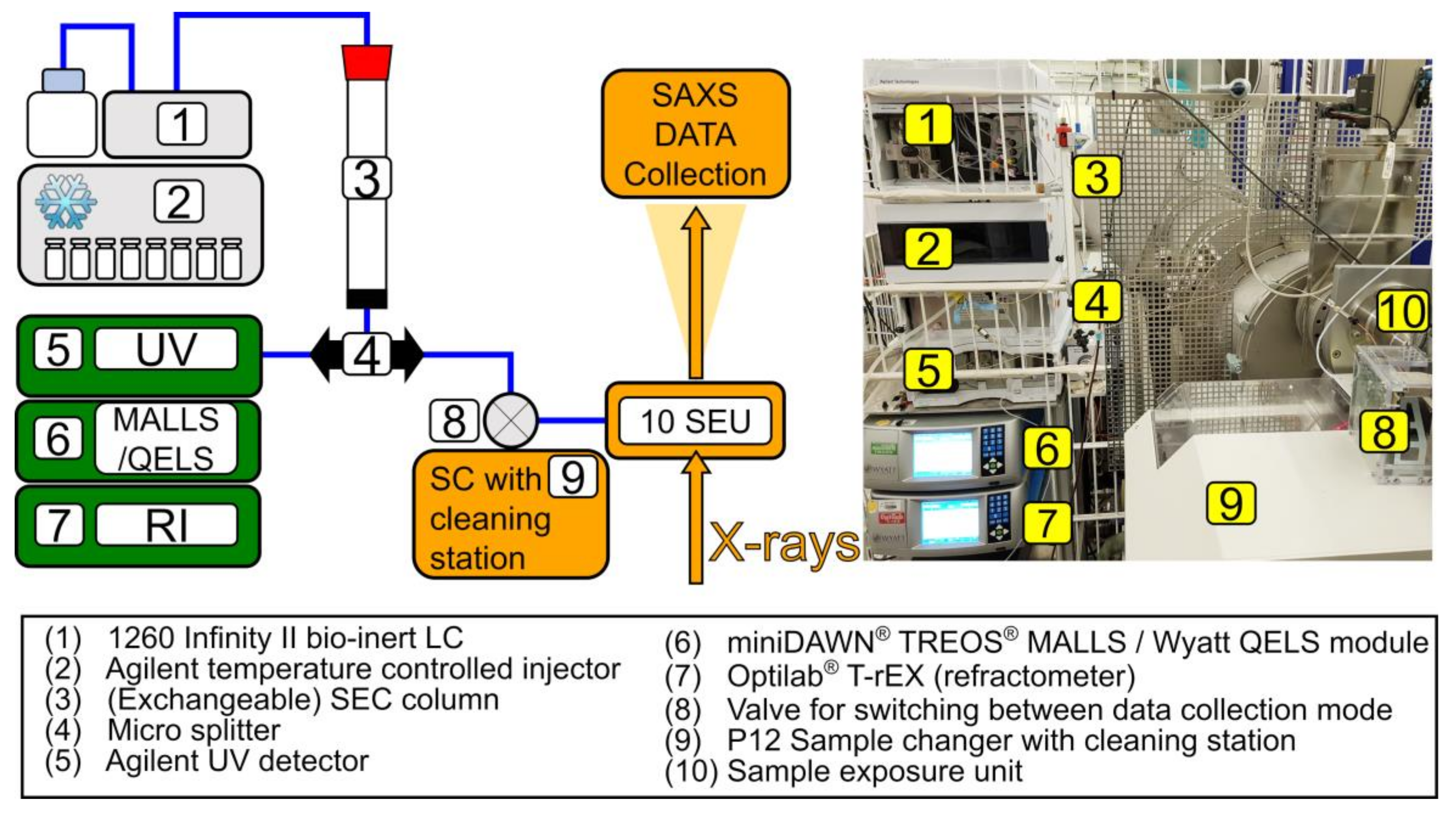
2.2. Experimental Set-Up

2.2.1. Chromatography System

The EMBL P12 beam line (PETRA III, DESY Hamburg, Germany [20]) is equipped with an Agilent 1260 Infinity II Bio-inert liquid chromatography system (LC, Agilent, Waldbronn, Germany). Three SEC-SAXS modes are available for user operations: (i) Basic SEC-SAXS, where the column outlet is connected directly to the SAXS measuring capillary; (ii) Serial SEC-UV-vis-SAXS, where the eluent is passed through an in-series UV-vis absorption spectrometer prior to the SAXS measurement capillary; and (iii) SEC-SAXS/MALLS, where the post-column eluent stream is split and passed in equal amounts to the SAXS capillary and the UV-vis, MALLS, and refractive index (RI) detectors, enabling parallel SAXS/LS data collection from the column eluent (Figure 1). For the studies described here, the SEC-SAXS/MALLS configuration was selected. Of note, a valve system is now in place to switch between the SEC-SAXS modes of operation and conventional batch SAXS measurements using the customized automated sample changer at the P12 beam line (Arinax, Moirans, France [21]). The custom-made beam line operating software BECQUEREL [22] has been designed to easily perform switching between batch- and SEC-SAXS, such as the remote control over valve, and it provides a common interface for both modes that includes the integrated control over the Agilent Chemstation LC software (Agilent Technologies, Santa Clara, CA, USA) and the coordinated communication of events between the LC system and SAXS data collection.
The LC system is compatible with a variety of both FPLC and HPLC SEC-columns routinely used for macromolecular separations, up to an operational pressure of 100 bar and higher, while also maintaining an appropriate flow rate to limit the effects of X-ray-induced radiation damage (at P12, flow >0.25 mL/min are required). In addition, the LC system is equipped with the Agilent 1260 Infinity Bio-Inert multisampler, which is designed for low sample carryover with an in-built sample-injection needle wash. It allows for the precise injection of volumes between 1 and 100 μL, and conventional (lidless) 1.5 mL reaction tubes (such as from Eppendorf, Germany) can be used (with an approximate dead volume of 5 μL). Care was taken to select connecting tubes leading to the SAXS capillary of the smallest feasible diameter, to avoid band broadening and a subsequent loss of resolution [23].
The injection volumes and concentrations of the CA, BSA, ADH, and aFER samples are listed in Table 1. For the SEC-SAXS/MALLS runs, a GE Superdex 200 Increase 10/300 column (GE Healthcare, Germany) was used, and the flow rate was set to 0.5 mL/min with the exception of CA, for which a GE Superdex 75 Increase 10/300 column was used. All columns were attached to a post-column 0.1 μm filter followed by a mobile-phase micro splitting valve, with low dead volume (P-451 Upchurch Scientific®, Figure 1 #4) to divert the eluent in two equal streams for the parallel acquisition of SAXS and MALLS/RI data (as described in Graewert et al. 2015 [13]). Splitting of the column eluent, as opposed to an in-line serial detection array, limits band broadening and remixing effects and the subsequent loss of separation resolution.

2.2.2. UV, MALLS, and RI Data Collection and Analysis

The UV-vis/MALLS/QELS/RI system at P12 consists of an Agilent variable wavelength UV-Vis detector (VWD) followed by a Wyatt (Wyatt, Germany) miniDAWN® TREOS® multi-angle laser light scattering detector (MALLS), with an in-built WyattQELS module and a Wyatt Optilab T-rEX (RI) refractometer. In all instances, UV absorption spectroscopy data were recorded at 280 nm. The MALLS system was calibrated relative to the light scattering of toluene for an absolute RI measurement of the mobile phase. The differential RI increment, dn/dc (mL/g), of each protein sample (Table 1) was calculated from the primary amino acid sequence using the method of Zhao et al. 2011 [24], which is integrated into the SEDFIT ‘vbar and dn/dc calculator’ [19], taking into account the experimentally determined RI of the solvent, measurement temperature (25 °C), and RI laser wavelength (658 nm). The molecular weight estimates, MWMALLS, were determined from the three-angle MALLS scattering intensities combined with the protein concentration determined from RI through the SEC elution peak of each sample using the ASTRA 7 software package (Wyatt Technology Corporation, Santa Barbara, CA, USA). In addition, the integrated QELS detector was used to evaluate the hydrodynamic radius, RH, of the protein samples in the mobile phase, with the incorporation of a correction for solvent viscosity due to the effect of 2% v/v glycerol in the running buffer. The viscosity of the 2% v/v glycerol running buffer was estimated at 0.9476 centipoise (cP) using the ‘Calculate density and viscosity of glycerol/water mixtures’ calculator [25] based on an assumption that glycerol, and not the other buffer components, is primarily responsible for affecting the translational diffusion coefficient of the proteins in solution compared to its value in water.

2.3. SAXS Data Collection and Reduction

The portion of the SEC column eluent used for SAXS measurements, under continuous flow, was directed into a 1 mm diameter quartz capillary housed within the in-vacuum beam line sample exposure unit. A capillary with 0.9 mm inner diameter has become the standard measurement cell, compared to the previous 1.7 mm option, as the narrower diameter increases the linear speed of the SEC eluent through the X-ray beam, reducing the chances of radiation damage [26]. In addition, the band broadening effect of the sample is lessened in the 0.9 mm capillary, improving the correlation between the background-corrected SAXS intensity at zero angle, I(0), and concentration estimates from the parallel UV-vis or RI measurements. For the set of experiments described here, the SAXS data were collected using a Pilatus 6M detector at a sample-detector distance of 3 m and at an X-ray wavelength λ of 0.124 nm. The data were recorded as a sequential set of 2880 individual 1 s frames, corresponding to one column volume (CV) for each protein sample (48 min total). Each individual 2D image underwent data reduction (azimuthal averaging) and normalization to the intensity of the transmitted beam to generate 1D scattering profiles plotted as I(s) vs. s through the momentum transfer range of 0.05 < s < 6 nm−1 (where s = 4πsinθ/λ and 2θ is the scattering angle). The s-axis was calibrated relative to a silver behenate [27]. As a preventative measure, automated washing cycles of the capillary were performed between each SEC-SAXS column run to remove the potential and unintended build-up of non-specific debris on the capillary surface that may happen at the point of X-ray exposure (“capillary fouling”) (Figure 2).

2.4. SAXS (Automated) Data Processing and Analysis

2.4.1. Background Subtraction of the SEC-SAXS Data

At the P12 beam line, a quick assessment and preliminary result of a SEC-SAXS experiment is possible “on the fly”. The program CHROMIXS [28] has been integrated into the automated data processing pipeline, SASFLOW [29]. The pipeline workflow can be described as follows: (i) integration of 2D images from the detector; (ii) separation of the integrated 1D frames according to their run number; (iii) launch of the corresponding run number data in CHROMIXS (see below [28]); (iv) determination of sample peaks and buffer region for each run number; and (v) generation of averaged and subtracted scattering profiles. Therefore, the pipeline generates a number of ready-for-analysis SAXS profiles for each run number and elution peak, so that the final steps of data processing are identical to the standard SASFLOW “Sample Changer mode” [29]. Finally, the pipeline passes each subtracted SAXS pattern to a set of programs, performing the determination of the overall SAXS parameters (RG, MW, Dmax), as well as the calculation of the real-space distance distribution function (p(r) profile). Then, this information is piped to the DAMMIF ab initio bead modeling routine, which generates a “first look” P1-symmetry low-resolution model [30]. The obtained parameters and models are gathered together in a single summary XML table, enabling fully automated and interactive on-site SAXS studies.
The program CHROMIXS [28] plots an s-range limited integrated intensity versus frame number to generate the corresponding “SAXS chromatogram” (Figure 3). The default s-range of 0.1 nm−1 < s < 0.8 nm−1 was used for the integration to aid the visualization the major SEC-elution peak(s) on the chromatogram and evaluate the stability of the scattering signal recorded from the SEC running buffer. The automated CHROMIXS selection of frames recorded before or after the sample peak, corresponding to the buffer, were averaged and used for the subtraction of background scattering contributions from the sample peak frames. The automated buffer scattering selection was additionally verified by visual inspection to dismiss any kind of background drift throughout the SEC run, which may be caused by capillary fouling. To assess the homogeneity of the sample, the stability of the radius of gyration, RG, and concentration-independent MW estimates for each buffer-subtracted sample peak frame were assessed. For the former, the ATSAS program AUTORG [31] was used, running in the background of CHROMIXS. The MW estimates from CHROMIXS are by default based on the Porod volume [32], or, alternatively, the program may be configured to assess the concentration-independent MW from a combined scattering invariant approach utilizing Bayesian inference [33]. Those individual subtracted SAXS curves producing a consistent RG through the elution peak were scaled to the one data frame with the highest integrated intensity and then averaged to generate the final SAXS profile. CHROMIXS performs this scaling operation by default, as opposed to normalizing each individual data frame to a sample concentration and then averaging, because the sample concentration is constantly changing through the SEC elution. It is necessary to compare the SAXS chromatogram with the output from the UV/RI detectors first to obtain the concentration profile and then evaluate the I(0) (and not integrated SAXS intensity) to assess concentration-dependent MW estimates. The final buffer and sample profiles used for the generation of final averaged processed CHROMIXS data are recorded in the footer of the ASCII format (.dat) file, and for P12, additional metadata relating to the experiment (e.g., X-ray wavelength, sample to detector distance, column type, flow rate injection volume, initial sample concentration, etc.) are listed in the footer of each unsubtracted data frame.

2.4.2. SAXS Data Analysis

ATSAS 2.8 [30] was employed for further data analysis and modeling. The program PRIMUS [34] was used to perform Guinier analysis (lnI(s) versus s2) in the very low-angle regime from which the radius of gyration, RG, and I(0) was determined. The p(r) distributions were calculated using the indirect Fourier transform method implemented in GNOM [35] that provided additional estimation of RG, I(0) and the maximum particle dimension, Dmax. The concentration-independent MW estimates from the SAXS data were assed with the Bayesian interference approach described by Hajizadeh et al. 2018 [33] that includes the estimation of a MW credibility interval for each sample. The MW estimates obtained from other concentration-independent methods based on scattering data invariants are also reported: MW from the volume of correlation, Vc [36]; SAXMoW [32]; Size-and-shape (S&S [37]) and Porod-volume, Qp [30,32]. In addition, a concentration-dependent assessment of the MW was performed in a two-fold manner using the forward scattering I(0) of the final SAXS curve, which was normalized by the concentration estimates at the of the top of the sample elution peak maxima as determined from RI measurements. The forward scattering of BSA of known concentration measured in batch mode was also used for calibration [38]. The ab initio modeling of the proteins was performed using either DAMMIN or GASBOR and the fit to the experimental data from the high-resolution crystal structures were computed by CRYSOL [39].
The experimental SAXS data described here, as well as the models derived from them, were deposited to the SASBDB [17] with the accession codes listed in Table 2. The unsubtracted 1D SAXS data frames encompassing the entire SEC-SAXS run of each sample, and CHROMIXS RG estimates through the SEC-SAXS chromatogram peaks combined with the UV-vis, MALLS, RI, and QELS data have also been deposited to the data bank.

2.4.3. Data Presentation

Python scripts were designed to use MatPlotLib and generate plots for quick visualization of the results. These quick-plot tools are accessible at the P12 beamline and can be used to evaluate measurement performance, allowing the possibility to adjust the collection strategy if required. Settings to produce high-quality figures for publications are also part of this tool kit.

3. Results

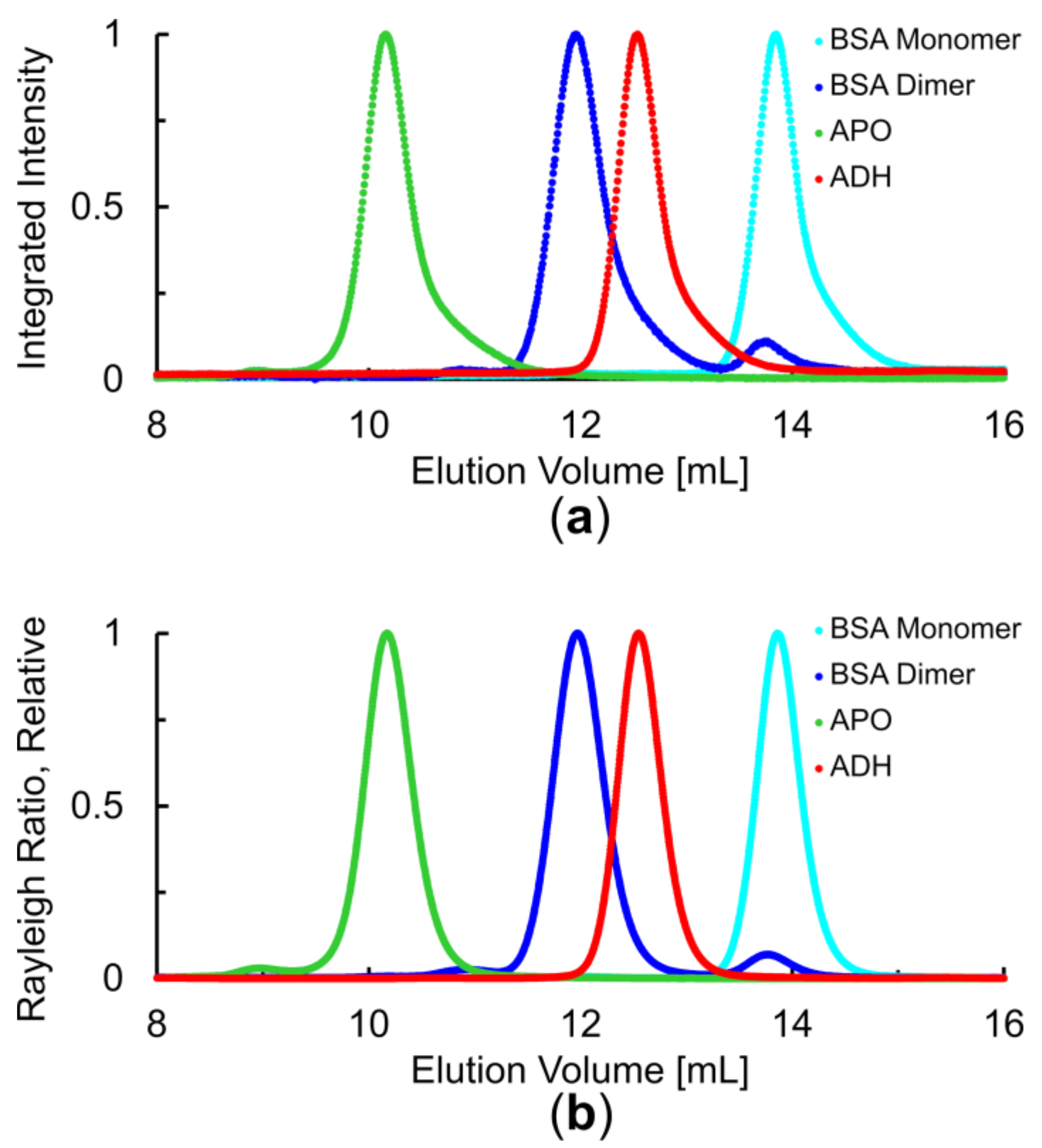
3.1. Overall Assessment of SEC Performance

Data were collected in SEC-SAXS/MALLS mode from five different standard proteins. In Figure 3, the CHROMIXS SEC-SAXS chromatogram results obtained from the monomeric and dimeric BSA samples, ADH, and aFER runs using a S200 Increase SEC-column (10/300) are overlaid and compared to the respective Rayleigh ratio chromatograms measured using MALLS (Figure 3b). The analogous elution profiles corresponding to CA, separated on an S75 Increase column, are shown in Supplement Figure S1. All five runs show a symmetrical major elution peak, and there is a strong correspondence between the SEC-SAXS chromatograms and the light-scattering results, demonstrating that the majority of the protein volume fraction of each individual sample, after dilution through the SEC column, presents as one isolatable oligomeric species. Only very minor pre- or post-peaks are noted corresponding to trace volume fractions of higher or lower oligomeric species in the injected samples. Notably, for the dimeric BSA (Figure 3, blue trace), a minor second peak indicates the presence of monomeric BSA, which cannot be avoided due to the dimer–monomer equilibrium of this protein. For SEC-SAXS, a tailing of the main peaks noted in the SAXS chromatograms are more prominent than for the SEC-MALLS traces. This can be explained by the band-broadening effect of the sample in the flow path caused by changes in the internal diameter (i.d.) of the tubing connecting the column outlet to the beam line: from the 50 μm i.d PEEK (polyether ether ketone) tubing connecting the column outlet to the SEC valve, through a short 120 μm i.d. adapter, and finally to the 0.9 mm i.d. SAXS capillary.
The absence of any traceable amount of aggregates that would otherwise flow through the SEC column void volume, or any multiple unresolved peaks in the SAXS chromatograms and LS traces, reflects the high quality of the samples prepared prior to the SEC-SAXS experiments. Although time-dependent aggregation may not be avoidable for other types of macromolecular samples (for which SEC-SAXS is an invaluable tool), it is important to remember that SEC-SAXS is as much an analytical technique as SEC-MALLS, requiring high-quality samples to obtain high-quality results. The SEC step at a beam line should not be used as a simple or quick substitute for the final step of a purification protocol. The quality of the sample should be taken into consideration prior to SEC-SAXS, which is why the samples described here all underwent a pre-purification step prior to measurement.
In all five runs, the integrated SAXS intensities of the SAXS chromatograms recorded toward the end of the SEC elution returned to a constant baseline (Figure 3, Supplement Figure S1). This has three important implications: (i) the column was sufficiently equilibrated prior to the experiment, the mobile phase was well matched to the sample solvent composition, and the column was not overloaded; (ii) no clear presence of X-ray-induced capillary fouling occurred during the course of the SEC-SAXS run, either damage to the buffer or to the proteins; (iii) the X-ray beam remained stable throughout the run, and the data were correctly normalized to the transmitted beam to accurately take into account both buffer and sample X-ray absorption.
The choice of mobile phase for SEC-SAXS should be guided by both the physical/chemical stability of the sample in the supporting solvent and the final X-ray contrast, column separation resolution, and the susceptibility of the sample toward X-ray-induced damage that may result in sample aggregation and subsequent capillary fouling. Capillary fouling caused by deposit build-up during the course of a SEC-SAXS run is a complicated process involving free radical, solvated electron, and quartz glass surface chemistries with the mobile phase and/or the macromolecule(s) of a sample, and is difficult to predict a priori. The implementation of co-FLOW SEC-SAXS, for example at the Australian Synchrotron SAXS beam line [40], mitigates such an effect. However, for SEC-SAXS in general, what may be considered as a “default” SEC purification buffer, e.g., phosphate-buffered saline, may not always be compatible with the X-ray properties/behavior of the sample in the X-ray beam. For example, and for the samples described here, 5 mM urea combined with low-salt (50 mM NaCl) and 1% v/v glycerol were included in the purification steps to (qualitatively) minimize aggregate formation during the comparatively long time frame of sample handling, purification, snap freezing, −80 °C storage, and defrosting, leading up to the SEC-SAXS experiments. The selected mobile phase for SEC-SAXS was based on the purification buffer, but it was modified for the final experiments so as to maximize the X-ray contrast while at the same time taking into account the effects of radiation damage, SEC column separation efficiency, and interparticle interactions. The final mobile phase included an increased percentage v/v of glycerol to help limit radiation damage [25,41] and an increased concentration of NaCl (150 mM) to help minimize the non-specific interactions of the proteins with the SEC column stationary phase (to improve separation resolution) and to decrease the possible contribution of Columbic repulsive interparticle interference effects in the final SAXS profiles.
Slight discrepancies in the buffer composition of the injected sample (loaded in the “preparation buffer”) compared to the SEC-SAXS mobile phase (in “SAXS buffer”) are often tolerable because most samples undergo on-column buffer exchange during the course of the elution. Any small molecule differences become detectable at the end of a SEC-SAXS run as the small buffer components derived from the injected sample take the longest diffusional path through the column matrix and typically elute slightly before one entire column volume. The presence of these small molecule differences is often detected by wild fluctuations in the RI signal (and often not UV absorption; Supplement Figure S2) recorded toward the end of the total elution of the sample. Therefore, it is generally advised to avoid selecting the “end of column” data frames from the corresponding region of the SAXS chromatogram for background scattering subtraction purposes, as these may differ with respect to X-ray contrast and X-ray absorption properties compared to the bulk mobile phase of the SEC run.

3.2. Concentration Determinion via UV Absorption and/or dRI

Knowing the eluent concentration (c) is essential for determining the MWMALLS and, independently, the MWI(0) from SAXS. The UV-vis/RI set-up allows for the protein concentration at every measurement point to be retrieved. For the UV-vis absorption-based concentration estimates, knowledge of the extinction coefficient at the employed wavelength is required as well as the optical path length of the UV-vis detector. For example, the extinction coefficient of proteins (E280) is typically determined at A280 nm from the amino acid sequence, which in most cases is sufficiently accurate to obtain reasonable concentration estimates. However, absorption-based methods necessitate that the macromolecule has sufficient chromophores to generate an absorption profile, which for proteins usually requires the presence of aromatic amino acids when measuring absorption at 280 nm. The RI-derived concentration determination is more widely applicable compared to UV-vis absorption for protein work, as it does not depend on the presence of absorbing species. In general, the differential refractive index, dn/dc, of proteins is more robust against changes in amino acid sequence compared to UV absorption [18] such that the dn/dc for most proteins—including those lacking aromatic amino acids—and without any conjugated molecules (e.g., glycoproteins, lipoproteins, etc.) can be first estimated at 0.185 mL/g at the laser wavelength of the Wyatt T-rEX (658 nm). The calculated dn/dc of a protein may be further adjusted as described by Zhao et al. 2011 [24] by taking the experimental absolute RI of the solvent (also obtained from the Wyatt TREX) and combining this value with the protein amino acid sequence, temperature, and laser wavelength information. The E280 extinction coefficients and adapted dn/dc values for the protein samples are listed in Table 1. In Table 2, the averaged concentration of the samples calculated for the final profiles are reported. Due to the rather large column volume (24 mL), the samples undergo a marked dilution by a factor of 6–10 compared to the sample injection concentration. When choosing the column for SEC-SAXS, one has to consider the tradeoff between separation power, which is often improved by longer columns or larger column volumes, and the associated dilution effect that is amplified when using larger columns. The dilution of the sample impacts both the intensity and variance (lowers the signal-to-noise ratio) of the resulting SAXS signal (as I(s) α c) and is especially relevant in cases where the oligomerization and/or the association of a fully formed protein complex is concentration dependent, as is demonstrated here by the disassociation of the BSA dimer sample on the column into a mixture of BSA monomers and dimers (Figure 3, blue curve).

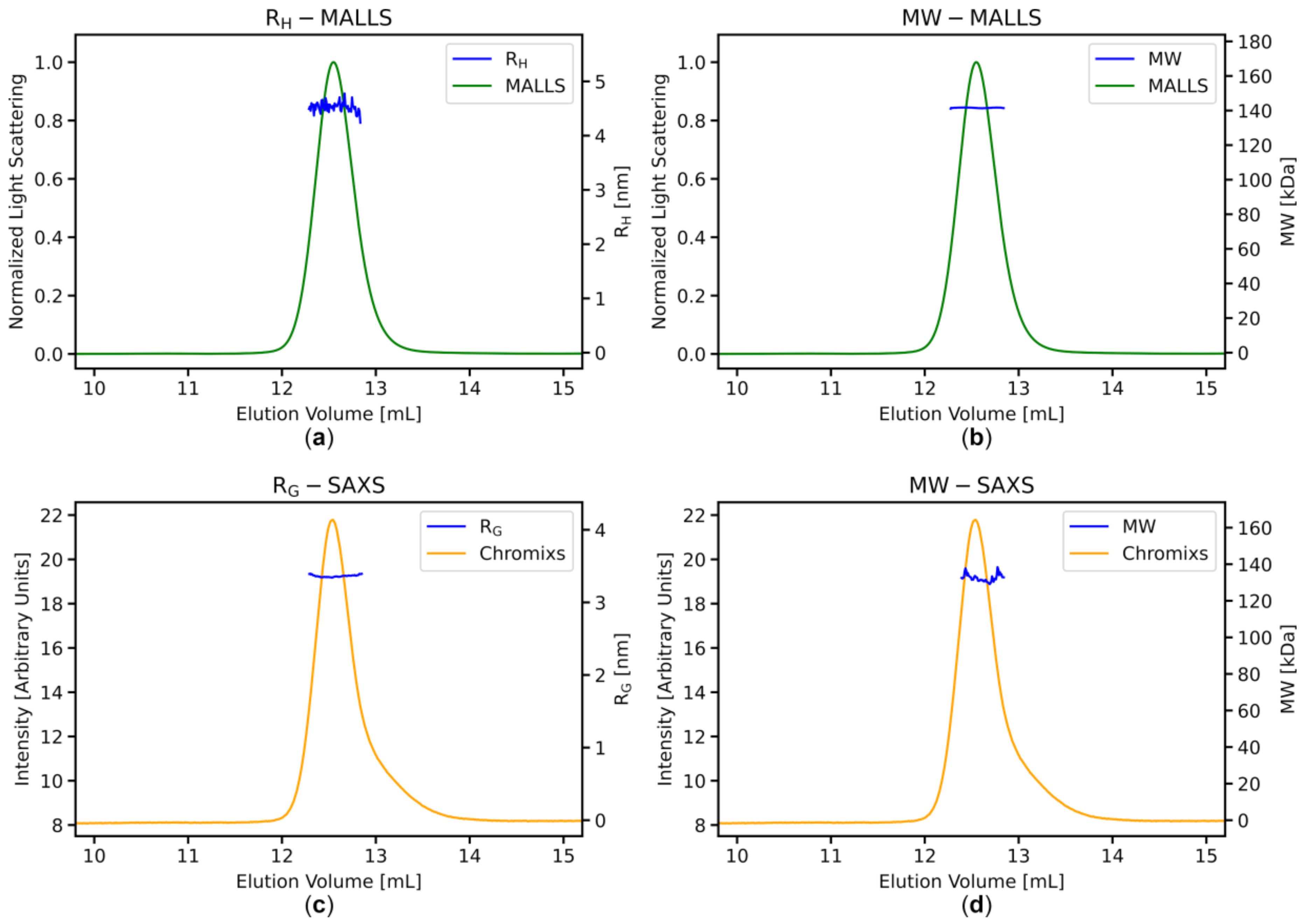
3.3. Stable MWMALLS and RH Estimates Across the Elution Peaks Indicate Homogeneous Sample Populations

The individual SEC-MALLS and QELS datasets were analyzed in relation to assessing the sample population homogeneity across the major elution peaks. In Figure 4a,b, the derived chromatograms for the ADH sample are displayed, showing the MW correlation obtained from the MALLS and RI measurements as well as the RH from QELS. An example of the QELS autocorrelation function from ADH is shown in Supplement Figure S3. For these calculations, the estimated viscosity of the SEC mobile phase due to the addition of 2% v/v glycerol was taken into account. The chromatograms of the other samples are provided in Supplementary Figures S4–S7. In combination, the light-scattering and subsequent stable MW and RH correlations demonstrate the homogeneity of the protein samples within the selected elution range from the SEC column (Table 2, Figure 4a, and Supplement Figures S4–S7).
When using SEC-MALLS, the MWMALLS estimate is independent of the elution behavior of the sample. Throughout a SEC run, the Rayleigh ratio—defined by the ratio of intensities of incident and scattered laser light at a specified distance—is both calibrated (in this case relative to toluene) and measured along with the concentration of the protein sample in the eluent, as determined by UV absorption or RI. This allows the Rayleigh ratio to be normalized by concentration to obtain the MW estimate. Alternatively, and more simply, SEC estimations of the MW that are not coupled to a LS system are often based on comparing the elution volume of a sample relative to elution volume of a set of protein standards with a known MW. However, the “elution volume only” approach is based on the underlying assumption that the sample in question displays the same hydrodynamic behavior as the measured standards and that the sample does not interact with the column matrix. For example, it may be the case for proteins with a more loosely packed structure compared to the calibration standards that the elution from the column is delayed, leading to an underestimation of the MW, whereas densely packed structures may elute sooner, suggesting a higher MW. Here, for example, the dimeric BSA (expected MW = 133 kDa) elutes unexpectedly at an earlier time point than the slightly heavier ADH (expected MW = 147 kDa, Figure 3). MW estimates based on elution volume alone may lead to inaccurate conclusions. In effect, both the MW and overall hydrodynamics/conformational state of the protein (compact, intrinsically disordered, rod-shaped, etc.) as well as sample/matrix interactions may contribute to elution–volume behavior. Figure 5 shows the ratio of the experimentally determined average MWMALLS estimates compared to the expected MW, MWexp, calculated from the amino acid sequence and known oligomeric state of the proteins (full squares). For the five examined proteins, these ratios are between 0.95 and 1.0 (Table 2).
The current configuration of the SEC-SAXS/MALLS set-up also includes the integrated Wyatt QELS module that allows the collection of dynamic light scattering data while the sample is eluting through the same measurement cell as used for MALLS. The ASTRA software allows for solvent viscosity corrections, e.g., the presence of glycerol, to model the RH from the measured auto correlation functions. From the derived autocorrelation function recorded at each time point through the elution, the distribution of RH across the elution peak can be examined (Table 2, Figure 4b and Supplement Figures S4–S7). From the stable correlation of RH across the elution peaks observed here, one can conclude that the samples stream as homogeneous populations with respect to the MW and also hydrodynamics. The presence of structural heterogeneity within a sample may manifest in a “tailing” of the elution peak where specific conformational states have a tendency to interact differently with the column matrix, leading to a delay in sample elution that may be identified by a change in RH. This additional biophysical characterization, both MALLS and QELS, is an asset when continuing SAXS data analysis, i.e., the selection of the appropriate data frames, and to inform subsequent interpretation (e.g., anisometry, the choice of oligomeric state used for ab initio and rigid-body modeling; the choice of flexible ensemble approaches, etc.).

3.4. SAXS Data Analysis: Stable RG and MWI(0) Estimates across the Elution Peaks

For all of the benchmark protein samples, the resulting CHROMIXS SAXS chromatograms show one major symmetrical peak with the return to a stable baseline and the baseline separation of the major peak from any minor species present in the injected samples. As a result, CHROMIXS is able to effectively delineate the major sample and buffer regions of the chromatogram and automatically process the final SEC-SAXS profile (Supplement Figure S8). In instances where the elution peaks are not well separated, or if there is significant drift in the integrated baseline scattering intensity, CHROMIXS may struggle to identify sample or buffer frames, and it may even return a message that it is not possible to find an adequate buffer region for subtraction purposes. For the SEC-SAXS pipeline at P12, the inability of CHROMIXS to automatically select the appropriate regions of the SAXS chromatogram will prevent further data analysis and on-the-fly “first look” ab initio modeling routines, and the user has to select and process the chromatogram manually through the CHROMIXS interface.
The CHROMIXS estimates of RG calculated for each individual frame through the selected sample range of the SAXS chromatogram are shown in (Figure 4c,d and Supplement Figures S4–S7). All five runs showed stable RG correlation for each of the five samples of the major elution peaks. CHROMIXS also includes a fast assessment of the MWChromixs for each sample frame which, as reported here, is based on the Porod volume estimate. In combination, the stability of the RG and MW correlations from SAXS and the MWMALLS and RH from QELS goes toward confirming the homogeneity of the eluting proteins and, importantly, that the intense X-ray beam has not damaged the protein samples as they flow through the SAXS capillary (Figure 4). With both the RG from SAXS and RH from QELS at hand, it is also possible to quickly calculate the shape factor, or RG/RH ratio, that provides a “parameter insight” into the conformation of the proteins in solution. The RG/RH for compact globular proteins is ≈0.78 and trends to higher values when the molecules deviate from globular to elongated structures. The shape factor obtained for the five proteins span 0.75 for CA—a very compact protein—to 0.86 for the BSA dimer, which may suggest a level of structural anisotropy. Without modeling the data, the general shape factor for all of the proteins indicate that they are all relatively globular species in solution (Table 2).

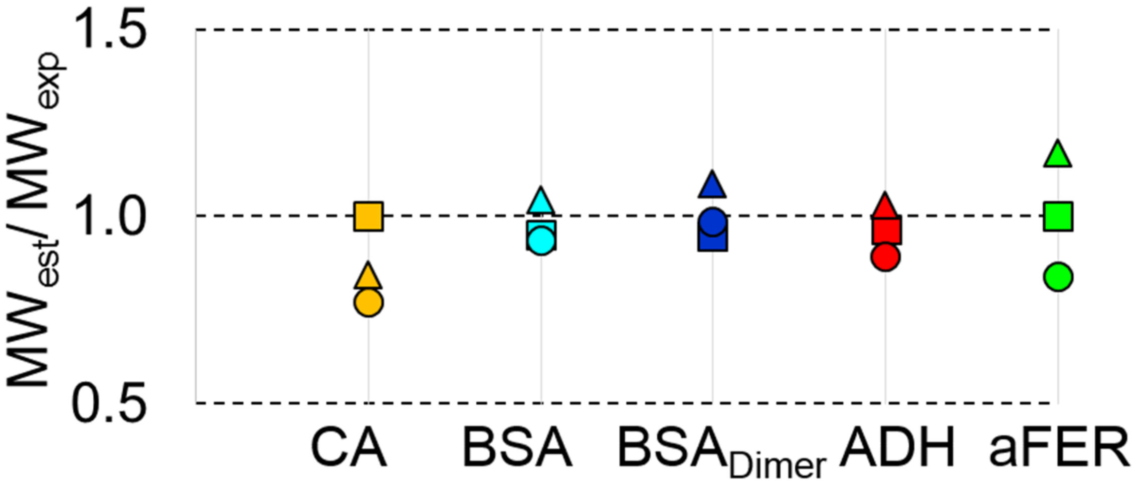
3.5. MWMALLS is the Most Robust Estimate for Determining the Molecular Weight for SEC-SAXS Applications

The determination of concentration-independent MW estimates using scattering invariant approaches from the integration of normalized Kratky plots (I(s)s2 vs. s) or Vc plots (I(s)s vs. s) has become a routine procedure in SAXS analysis of non-conjugated protein-only samples. Here, we used the Bayesian interference approach [33] that combines several of these methods together to obtain the most probable estimated protein MW and MW credibility interval calculated directly from the scattering profiles (Table 2). All values are in close proximity to the expected MW.
Alternatively, the concentration-dependent MW estimate based on sample concentration and the forward scattering, MWI(0), was also determined, and the values are also in close approximation to the expected values. The advantage of this concentration-dependent method (either calibrated relative to a known protein standard—as was employed here—or via absolute scaling of the data [38]) is that it may be applied to macromolecules in general or macromolecular conjugates and is not dependent on the macromolecule shape. However, the disadvantage is the accurate assessment of the sample concentration that for bio-macromolecules is not always trivial, especially for SEC where the concentration of the eluting species is ever-changing and potentially affected by band-broadening in the SAXS capillary. However, by utilizing a split-eluent flow approach in the SEC-SAXS/MALLS set-up, and reducing the SAXS sample capillary diameter, the concentration at the point of X-ray exposure during the course of a SEC-SAXS run may be estimated using the UV and RI detectors set up in parallel to the SAXS measurements. For the visualization and quantification of the different MW approaches, the ratios of the various MW estimates to the expected MW are plotted in Figure 5. From this, we conclude that for the simple globular protein samples described here, both concentration-dependent and independent methods are consistent, although MWMALLS (full squares) appears as the most robust experimental method for validating the MW.

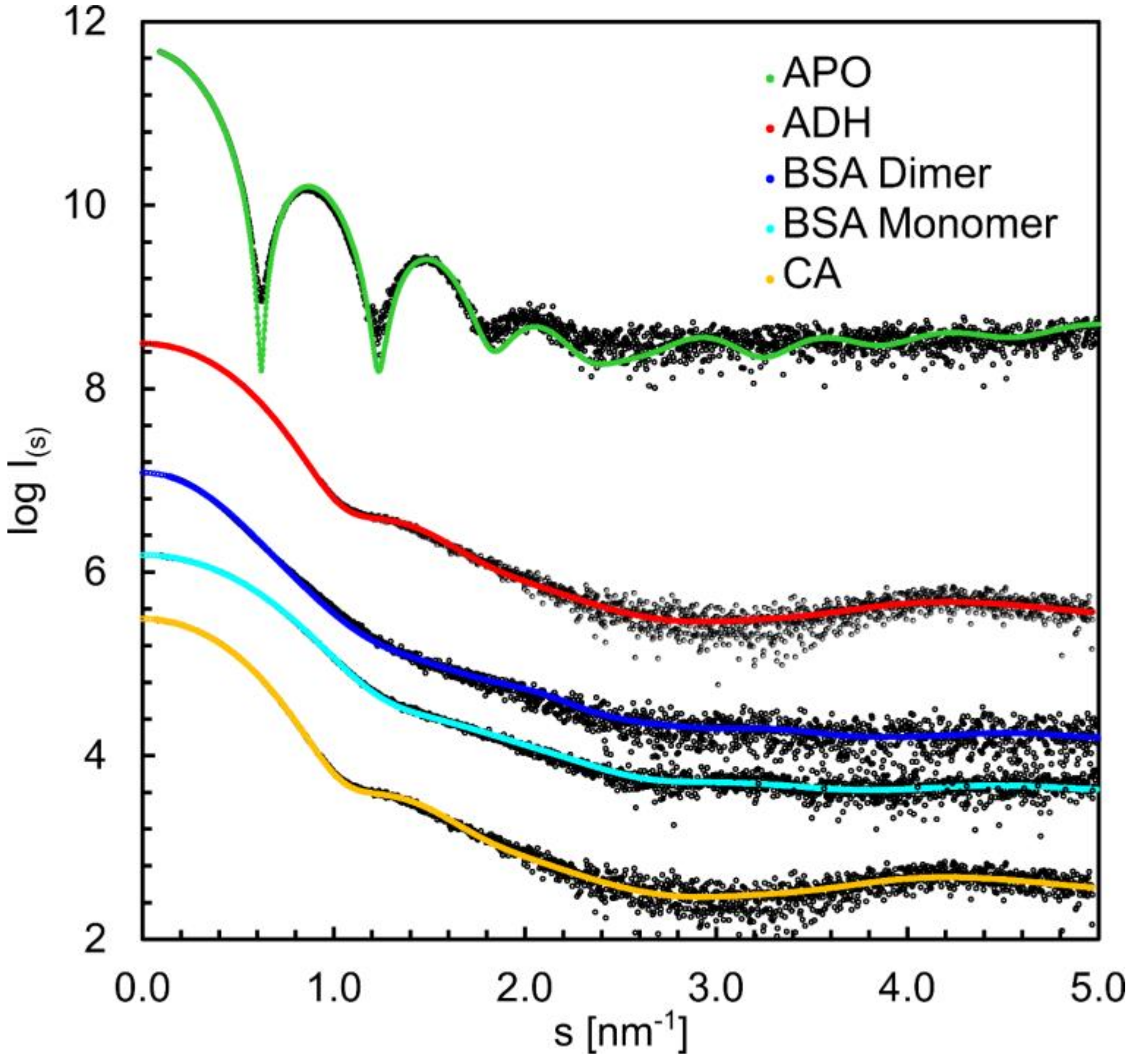
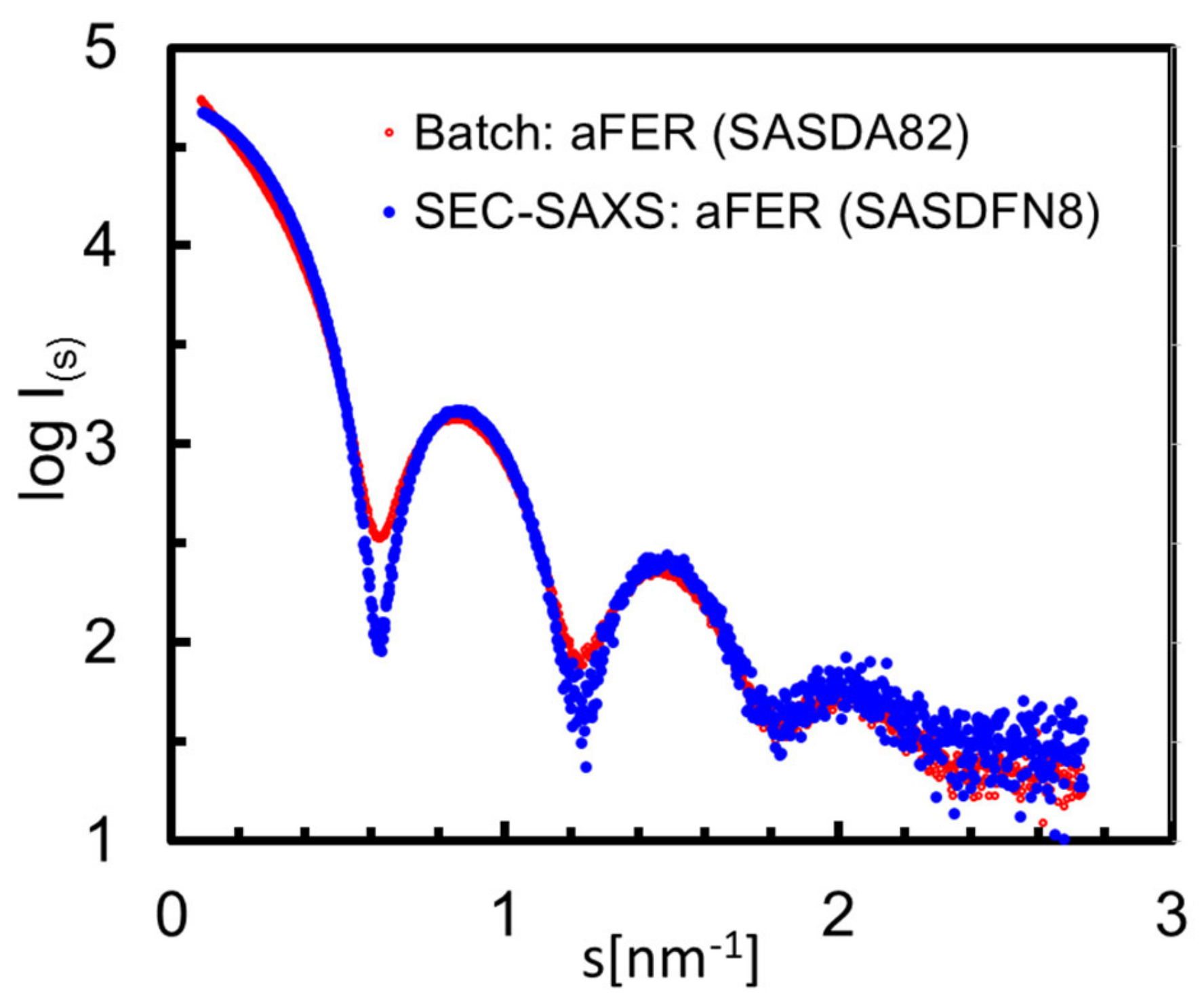
3.6. Structural Information Derived from the Buffer-Subtracted SAXS Scattering Curves

For all five proteins, atomistic models determined from X-ray crystallography are available. Theoretical scattering profiles were calculated from these models and compared to the experimental data with CRYSOL. The obtained χ2 values are listed in Table 2, and the visual inspection of the fits in Figure 6 suggest that the crystal structures are generally in reasonable agreement with the solution data. The strongest discrepancies with elevated χ2 values are observed for Apoferritin and dimeric BSA. The divergence of the former can partially be explained by small shape variations of the Apoferritin assembly in solution compared to the highly symmetric crystal structure. For the dimeric BSA, the scattering data suggest that the dimer in solution has a somewhat more extended monomer arrangement compared to the one observed in the crystal packing. The other curves show very good fits with χ2 values ranging from 1.1 to 1.4 (Table 2).

4. Discussion

Since the first installation of SEC-SAXS at the P12 beam line in 2012, demand for the technique has significantly increased. At present, 60% of P12 users make use of SEC-SAXS during their visits or request SEC-SAXS as part of mail-in operations. The current and ongoing improvements at the beam line have streamlined the processes of sample delivery, data acquisition, and analysis in step with this demand. The newest developments of the P12 system include:
(i)
Upgraded hardware modules such as the automated injector and switching valve for better use of allocated beamtime (the need to physically enter the experimental hutch by the operators is reduced, as several samples can be queued, and washing between samples can be initiated remotely).
(ii)
The robust HPLC pumps allow extensive use of columns (also at high pressures). Quaternary solvent blending offers increased flexibility in remote preparation of buffers e.g., varying in ionic strength or pH gradient.
(iii)
The additional acquisition of QELS data allows for further assessment of sample homogeneity (stability of RH across elution peak) as well as structural information through the RG/RH ratio.
(iv)
Collection of MALLS data at three angles provides more precise MWMALLS estimates.
(v)
A combination of software tools and a common beamline-control interface (BEQUEREL) for ease of use and the necessary communication between integrated devices during data collection [22] as well as for data analysis such as CHROMIXS [27] and the new QuickPlot tools described here. Evaluation of data quality “on the spot” can optimize beam time usage, as improving measures can be made for subsequent runs.
As demonstrated here, the quality of SAXS data can be increased significantly by the in-line SEC system, allowing the immediate acquisition of data after the individual components of a sample elute from a size exclusion column. Figure 7 displays the difference between batch data (taken from SASBDB entry SASDA82) and the SEC data described here for aFER. At higher angles, the two curves overlap well, but the minima in the curve measured with SEC are more pronounced, pointing to a cleaner system. At lower angles, the batch data show a faster descent and overall larger SAXS parameters (RG = 6.8 nm, Dmax = 12.8 nm), suggesting the presence of higher oligomeric species in the sample measured in batch mode.
Moreover, the analysis and interpretation of the SAXS data is greatly facilitated, and confidence in the subsequent conclusions increased, if the sample is additionally characterized biophysically with the multi-detector LS system. At this point, we would like to strongly emphasize that the SEC-SAXS step does not replace the need for preparing a high-quality sample. In addition, the success of the experiment depends on an optimized buffer and column selection.
The current improvements to the SEC-SAXS/MALLS set-up have allowed us to collect SAXS data with additional static and dynamic light scattering information for the purposes of benchmarking. These datasets have been deposited into the SASBDB [17] and are made available to the community for testing, development, critique, and interrogation. Screenshots of these entries are shown in Supplement Figures S9–S13.
Finally, we do not expect SEC-SAXS to make the classical batch mode of data collection obsolete. Batch mode SAXS has the advantage of very fast collection times, minimal sample volumes, and high-throughput screening possibilities. It is by far the most appropriate technique for the structural analysis of transient oligomers or low-affinity macromolecular complexes that would otherwise disassociate on an SEC column. As the biology is based on macromolecular association, even weak interactions may have functional relevance. Moreover, batch experiments allow for specific variations in concentration, pH, temperature, buffer additives, stoichiometric ratios, and many other biologically relevant parameters. Therefore, SEC-SAXS is not a “golden technique” to be routinely applied to all samples or experiments. Instead, this is a powerful analytical approach that is especially effective for systems notoriously difficult to keep in a purified state, and this approach is made even stronger by in-line biophysical characterization (absorption, light-scattering, and refractive index measurements).

Supplementary Materials

The following are available online at https://www.mdpi.com/2073-4352/10/11/975/s1, Figure S1: Elution profile of CA, Figure S2: Elution profile of aFER, Figure S3: Autocorrelation functions (ACFs), Figure S4: In detail characterization of CA, Figure S5: In detail characterization of monomeric BSA, Figure S6: In detail characterization of dimeric BSA, Figure S7: In detail characterization of aFER, Figure S8: Automated output summary from CHROMIXS/SASFLOW, Figure S9: SASDFP8—Carbonic anhydrase from bovine erythrocytes, Figure S10: SASDFQ8—Bovine serum albumin, purified monomer, Figure S11: SASDFR8—Bovine serum albumin, purified dimer, Figure S12: SASDFS8—Yeast alcohol dehydrogenase 1, Figure S13: SASDFN8—Apoferritin horse spleen.

Author Contributions

Conceptualization, S.D.V., D.I.S. and C.M.J.; Data curation, C.M.J.; Formal analysis, M.A.G., S.D.V., T.V.G., D.S.M., C.E.B. and C.M.J.; Funding acquisition, D.I.S.; Investigation, M.A.G., S.D.V. and C.M.J.; Methodology, M.A.G., S.D.V., T.W.G., D.S.M., C.E.B., D.I.S. and C.M.J.; Project administration, C.M.J.; Resources, D.I.S.; Software, T.W.G., D.S.M. and D.I.S.; Supervision, M.A.G., D.I.S. and C.M.J.; Validation, M.A.G., C.E.B. and C.M.J.; Visualization, M.A.G., T.W.G. and D.S.M.; Writing—original draft, M.A.G., T.W.G. and C.M.J.; Writing—review and editing, M.A.G., S.D.V., T.W.G., D.S.M., C.E.B., D.I.S. and C.M.J. All authors have read and agreed to the published version of the manuscript.

Funding

This work has been supported by iNEXT-Discovery, project number 871037, funded by the Horizon 2020 program of the European Commission. In addition, D.S.M. is supported by the German Ministry of Science and Education Grant Number: 16QK10A-SAS-BSOFT and S.D.V. acknowledges funding from the “Biomedical Physics of Infection” grant (no. 900000) of the Joachim Herz Stiftung (Hamburg, Germany).

Acknowledgments

We would like to thank the EMBL Hamburg Instrumentation team lead by Stefan Fiedler for their technical support.

Conflicts of Interest

The authors declare no conflict of interest.

References

  1. Tuukkanen, A.T.; Spilotros, A.; Svergun, D.I. Progress in small-angle scattering from biological solutions at high-brilliance synchrotrons. IUCrJ 2017, 4, 518–528. [Google Scholar] [CrossRef] [Green Version]
  2. Bernadó, P.; Shimizu, N.; Zaccai, G.; Kamikubo, H.; Sugiyama, M. Solution scattering approaches to dynamical ordering in biomolecular systems. Biochim. Biophys. Acta BBA Gen. Subj. 2018, 1862, 253–274. [Google Scholar] [CrossRef]
  3. Vallat, B.; Webb, B.; Westbrook, J.; Sali, A.; Berman, H.M. Development of a prototype system for archiving integrative/hybrid structure models of biological macromolecules. Structure 2018, 26, 894–904. [Google Scholar] [CrossRef] [Green Version]
  4. Brosey, C.A.; Tainer, J.A. Evolving SAXS versatility: Solution X-ray scattering for macromolecular architecture, functional landscapes, and integrative structural biology. Curr. Opin. Struct. Biol. 2019, 58, 197–213. [Google Scholar] [CrossRef] [PubMed]
  5. Jeffries, C.M.; Graewert, M.A.; Blanchet, C.E.; Langley, D.B.; Whitten, A.E.; Svergun, D.I. Preparing monodisperse macromolecular samples for successful biological small-angle X-ray and neutron-scattering experiments. Nat. Protoc. 2016, 11, 2122–2153. [Google Scholar] [CrossRef] [PubMed] [Green Version]
  6. Graewert, M.A.; Jeffries, C.M. Sample and Buffer Preparation for SAXS. Adv. Exp. Med. Biol. 2017, 1009, 11–30. [Google Scholar] [CrossRef] [PubMed]
  7. Mathew, E.; Mirza, A.; Menhart, N. Liquid-chromatography-coupled SAXS for accurate sizing of aggregating proteins. J. Synchrotron Radiat. 2004, 11, 314–318. [Google Scholar] [CrossRef] [PubMed] [Green Version]
  8. Watanabe, Y.; Inoko, Y. Size-exclusion chromatography combined with small-angle X-ray scattering optics. J. Chromatogr. A 2009, 1216, 7461–7465. [Google Scholar] [CrossRef]
  9. Pérez, J.; Vachette, P. A successful combination: Coupling SE-HPLC with SAXS. Adv. Exp. Med. Biol. 2017, 1009, 183–199. [Google Scholar] [CrossRef] [PubMed]
  10. Johansen, N.T.; Pedersen, M.C.; Porcar, L.; Martel, A.; Arleth, L. Introducing SEC–SANS for studies of complex self-organized biological systems. Acta Crystallogr. Sect. D Struct. Biol. 2018, 74, 1178–1191. [Google Scholar] [CrossRef]
  11. Bucciarelli, S.; Midtgaard, S.R.; Pedersen, M.N.; Skou, S.; Arleth, L.; Vestergaard, B. Size-exclusion chromatography small-angle X-ray scattering of water soluble proteins on a laboratory instrument. J. Appl. Crystallogr. 2018, 51, 1623–1632. [Google Scholar] [CrossRef]
  12. Inoue, R.; Nakagawa, T.; Morishima, K.; Sato, N.; Okuda, A.; Urade, R.; Yogo, R.; Yanaka, S.; Yagi-Utsumi, M.; Kato, K.; et al. Newly developed laboratory-based size exclusion chromatography small-angle X-ray scattering system (La-SSS). Sci. Rep. 2019, 9, 1–12. [Google Scholar] [CrossRef] [PubMed] [Green Version]
  13. Graewert, M.A.; Franke, D.; Jeffries, C.M.; Blanchet, C.E.; Ruskule, D.; Kuhle, K.; Flieger, A.; Schäfer, B.; Tartsch, B.; Meijers, R.; et al. Automated pipeline for purification, biophysical and X-ray analysis of biomacromolecular solutions. Sci. Rep. 2015, 5, 10734. [Google Scholar] [CrossRef]
  14. Jacques, D.A.; Guss, J.M.; Svergun, D.I.; Trewhella, J. Publication guidelines for structural modelling of small-angle scattering data from biomolecules in solution. Acta Crystallogr. Sect. D Biol. Crystallogr. 2012, 68, 620–626. [Google Scholar] [CrossRef] [PubMed] [Green Version]
  15. Trewhella, J.; Duff, A.P.; Durand, D.; Gabel, F.; Guss, J.M.; Hendrickson, W.A.; Hura, G.L.; Jacques, D.A.; Kirby, N.M.; Kwan, A.H.; et al. Publication guidelines for structural modelling of small-angle scattering data from biomolecules in solution: An update. Acta Crystallogr. Sect. D Struct. Biol. 2017, 73, 710–728. [Google Scholar] [CrossRef] [Green Version]
  16. Valentini, E.; Kikhney, A.G.; Previtali, G.; Jeffries, C.M.; Svergun, D.I. SASBDB, a repository for biological small-angle scattering data. Nucleic Acids Res. 2014, 43, D357–D363. [Google Scholar] [CrossRef] [PubMed] [Green Version]
  17. Kikhney, A.G.; Borges, C.R.; Molodenskiy, D.S.; Jeffries, C.M.; Svergun, D.I. SASBDB: Towards an automatically curated and validated repository for biological scattering data. Protein Sci. 2019, 29, 66–75. [Google Scholar] [CrossRef] [Green Version]
  18. Wilkins, M.R.; Gasteiger, E.; Bairoch, A.; Sanchez, J.-C.; Williams, K.L.; Appel, R.D.; Hochstrasser, D.F. Protein identification and analysis tools in the ExPASy server. Methods Mol. Biol. 1999, 112, 531–552. [Google Scholar] [CrossRef]
  19. Schuck, P. Size-distribution analysis of macromolecules by sedimentation velocity ultracentrifugation and lamm equation modeling. Biophys. J. 2000, 78, 1606–1619. [Google Scholar] [CrossRef] [Green Version]
  20. Blanchet, C.E.; Spilotros, A.; Schwemmer, F.; Graewert, M.A.; Kikhney, A.; Jeffries, C.M.; Frank, S.; Mark, D.; Zengerle, R.; Cipriani, F.; et al. Versatile sample environments and automation for biological solution X-ray scattering experiments at the P12 beamline (PETRA III, DESY). J. Appl. Crystallogr. 2015, 48, 431–443. [Google Scholar] [CrossRef]
  21. Round, A.; Felisaz, F.; Fodinger, L.; Gobbo, A.; Huet, J.; Villard, C.; Blanchet, C.E.; Pernot, P.; McSweeney, S.; Roessle, M.; et al. BioSAXS Sample Changer: A robotic sample changer for rapid and reliable high-throughput X-ray solution scattering experiments. Acta Crystallogr. Sect. D Biol. Crystallogr. 2015, 71, 67–75. [Google Scholar] [CrossRef] [PubMed] [Green Version]
  22. Hajizadeh, N.R.; Franke, D.; Svergun, D.I. Integrated beamline control and data acquisition for small-angle X-ray scattering at the P12 BioSAXS beamline at PETRAIII storage ring DESY. J. Synchrotron Radiat. 2018, 25, 906–914. [Google Scholar] [CrossRef] [PubMed] [Green Version]
  23. Grinias, J.P.; Bunner, B.; Gilar, M.; Jorgenson, J.W. Measurement and Modeling of Extra-Column Effects Due to Injection and Connections in Capillary Liquid Chromatography. Chromatography 2015, 2, 669–690. [Google Scholar] [CrossRef] [Green Version]
  24. Zhao, H.; Brown, P.H.; Schuck, P. On the distribution of protein refractive index increments. Biophys. J. 2011, 100, 2309–2317. [Google Scholar] [CrossRef] [Green Version]
  25. Volk, A.; Kähler, C.J. Density model for aqueous glycerol solutions. Exp. Fluids 2018, 59, 75. [Google Scholar] [CrossRef] [Green Version]
  26. Schroer, M.A.; Blanchet, C.E.; Gruzinov, A.Y.; Gräwert, M.A.; Brennich, M.E.; Hajizadeh, N.R.; Jeffries, C.M.; Svergun, D.I. Smaller capillaries improve the small-angle X-ray scattering signal and sample consumption for biomacromolecular solutions. J. Synchrotron Radiat. 2018, 25, 1113–1122. [Google Scholar] [CrossRef] [PubMed] [Green Version]
  27. Huang, T.C.; Toraya, H.; Blanton, T.N.; Wu, Y. X-ray powder diffraction analysis of silver behenate, a possible low-angle diffraction standard. J. Appl. Crystallogr. 1993, 26, 180–184. [Google Scholar] [CrossRef] [Green Version]
  28. Panjkovich, A.; Svergun, D.I. CHROMIXS: Automatic and interactive analysis of chromatography-coupled small-angle X-ray scattering data. Bioinformatics 2017, 34, 1944–1946. [Google Scholar] [CrossRef]
  29. Franke, D.; Kikhney, A.G.; Svergun, D.I. Automated acquisition and analysis of small angle X-ray scattering data. Nucl. Inst. Meth. A 2012, 689, 52–59. [Google Scholar] [CrossRef]
  30. Franke, D.; Svergun, D.I. DAMMIF, a program for rapid ab-initio shape determination in small-angle scattering. J. Appl. Crystallogr. 2009, 42, 342–346. [Google Scholar] [CrossRef] [Green Version]
  31. Franke, D.; Petoukhov, M.V.; Konarev, P.V.; Panjkovich, A.; Tuukkanen, A.; Mertens, H.D.T.; Kikhney, A.G.; Hajizadeh, N.R.; Franklin, J.M.; Jeffries, C.M.; et al. ATSAS 2.8: A comprehensive data analysis suite for small-angle scattering from macromolecular solutions. J. Appl. Crystallogr. 2017, 50, 1212–1225. [Google Scholar] [CrossRef] [PubMed] [Green Version]
  32. Fischer, H.; Neto, M.D.O.; Napolitano, H.B.; Polikarpov, I.; Craievich, A.F. Determination of the molecular weight of proteins in solution from a single small-angle X-ray scattering measurement on a relative scale. J. Appl. Crystallogr. 2009, 43, 101–109. [Google Scholar] [CrossRef]
  33. Hajizadeh, N.R.; Franke, D.; Jeffries, C.M.; Svergun, D.I. Consensus Bayesian assessment of protein molecular mass from solution X-ray scattering data. Sci. Rep. 2018, 8, 1–13. [Google Scholar] [CrossRef] [PubMed]
  34. Konarev, P.V.; Volkov, V.V.; Sokolova, A.V.; Koch, M.H.J.; Svergun, D.I. PRIMUS: A Windows PC-based system for small-angle scattering data analysis. J. Appl. Crystallogr. 2003, 36, 1277–1282. [Google Scholar] [CrossRef]
  35. Svergun, D. Determination of the regularization parameter in indirect-transform methods using perceptual criteria. J. Appl. Crystallogr. 1992, 25, 495–503. [Google Scholar] [CrossRef]
  36. Rambo, R.P.; Tainer, J.A. Accurate assessment of mass, models and resolution by small-angle scattering. Nat. Cell Biol. 2013, 496, 477–481. [Google Scholar] [CrossRef] [PubMed]
  37. Franke, D.; Jeffries, C.M.; Svergun, D.I. Machine learning methods for X-ray scattering data analysis from biomacromolecular solutions. Biophys. J. 2018, 114, 2485–2492. [Google Scholar] [CrossRef] [Green Version]
  38. Mylonas, E.; Svergun, D.I. Accuracy of molecular mass determination of proteins in solution by small-angle X-ray scattering. J. Appl. Crystallogr. 2007, 40, s245–s249. [Google Scholar] [CrossRef] [Green Version]
  39. Svergun, D.; Barberato, C.; Koch, M.H.J. CRYSOL—A program to evaluate X-ray solution scattering of biological macromolecules from atomic coordinates. J. Appl. Crystallogr. 1995, 28, 768–773. [Google Scholar] [CrossRef]
  40. Kirby, N.; Cowieson, N.; Hawley, A.M.; Mudie, S.T.; McGillivray, D.J.; Kusel, M.; Samardzic-Boban, V.; Ryan, T.M. Improved radiation dose efficiency in solution SAXS using a sheath flow sample environment. Acta Crystallogr. Sect. D Struct. Biol. 2016, 72, 1254–1266. [Google Scholar] [CrossRef]
  41. Jeffries, C.M.; Graewert, M.A.; Svergun, D.I.; Blanchet, C.E. Limiting radiation damage for high-brilliance biological solution scattering: Practical experience at the EMBL P12 beamline PETRAIII. J. Synchrotron Radiat. 2015, 22, 273–279. [Google Scholar] [CrossRef]
Figure 1. Size-exclusion chromatography small angle X-ray scattering (SEC-SAXS)/multi-angle laser light scattering (MALLS) station at European Molecular Biology Laboratory (EMBL)s 12 beamline (PETRA III @ DESY, Hamburg, Germany. Left, schematic drawing. Right, photograph. Individual modules are indicated.
Crystals 10 00975 g001
Figure 2. Overview of the automated analysis procedure for SEC-SAXS data collected at P12.
Crystals 10 00975 g002
Figure 3. Overlaid elution profiles of indicated samples from Superdex 200 increase 10/300 column at 0.5 mL/min collected in SEC-SAXS/MALLS mode. (a) SAXS-derived chromatogram—integrated intensities (0.1 nm−1 < s < 0.8 nm−1) vs. elution volume. (b) MALLS-derived chromatogram—Rayleigh Ratio (90°) vs. elution volume. Profiles on relative scale for better comparison. Note, CA is shown separately in Supplement Figure S1. Protein samples are indicated and correspond to the corresponding SASBDB accession codes: BSA monomer (SASDFQ8), BSA dimer (SASDFR8), APO (SASDFS8), and ADH (SASDFN8).
Crystals 10 00975 g003
Figure 4. In detail characterization of alcohol dehydrogenase (ADH) elution profiles. (a,b) MALLS derived chromatogram—Rayleigh Ratio vs. elution volume in green with stable RH (a) and MWMALLS (b) across the elution peak. (c,d) SAXS-derived chromatogram-integrated intensities vs. elution volume produced by CHROMIXS (in orange) with stable RG values across the elution peak (c) and Porod volume-derived MW estimate (d). Identical figures for the other four samples are shown in Supplement Figures S2–S5.
Crystals 10 00975 g004
Figure 5. A comparison of the experimentally determined MW estimates from MALLS and SAXS in terms of the ratio with the expected/calculated MW of each protein. Depicted are the ratios of MWMALLS (squares), MWBayesian (circles), as well as MWI(0) (calibrated with scattering of BSA as standard; triangles) over MWexp, taking into account the oligomerization state of each protein sample.
Crystals 10 00975 g005
Figure 6. Validation of atomistic structures in solution. Final I(s) vs. s scattering curves are fitted by the theoretical scattering curves of available pdb structures. Subtracted SAXS profiles shown in log-linear plot and shifted along the y-axis for better visibility. PDB files and resulting χ2 values are listed in Table 2.
Crystals 10 00975 g006
Figure 7. Comparison of SAXS data collected in Batch mode with the SEC-SAXS data described here. The SASBDB entries are indicated.
Crystals 10 00975 g007
Table 1. Sample overview.
SampleCarbonic Anyhdrase 2Serum AlbuminSerum Albumin (dimer)Alcohol DehydrogenaseApoferritin
AbbreviationCABSABSA dimerADHaFER
SourceBos tauruserythrocytesBos taurusBos taurusSaccharomyces cerevisiaeEquus caballus
Oligomeric stateMonomerMonomerDimerTetramerTetramer
Calculated MW *29 kDa66 kDa133 kDa147 kDa454 kDa
SEC-SAXS buffer50 mM HEPES, 150 mM NaCl, 2% v/v glycerol, pH 7
SEC-SAXS columnSuperdex 75 inc. 10/300Superdex 200 increase, 10/300
SEC-SAXS injection volume100 μL100 μL100 μL100 μL50 μL
SEC-SAXS injection concentration11.9 mg/mL8.8 mg/mL5.5 mg/mL9.2 mg/mL11 mg/mL
A280 nm Extinction coefficient, E0.1% **1.7320.6460.6461.3260.729
dn/dc (mL/g) ***0.18700.18520.18520.18420.1860
UniProt entry
(amino acid sequence range)
P00921
(1-260)
P02769
(25-607)
P02769
(25-607)
P00330
(1-348)
P02791
(1-175)
* From amino acid sequence and oligomeric state. ** E 0.1% (=1 g/L) calculated from the amino acid sequence (ProtParam [18]). *** dn/dc was estimated using the ‘vbar and dn/dc calculator’ module of SEDFIT [19] based on the primary amino acid sequence of each protein taking into account the experimentally determined average absolute refractive index (RI) of the solvent (1.3380), temperature (25 °C), and RI laser wavelength (658 nm).
Table 2. SAXS data collection, statistics, and overview of biophysical and SAXS-derived parameters.
CABSABSA DimerADHaFER
Data Collection Parameters
InstrumentEMBLP12 (PETRAIII, DESY, Hamburg)
Beam geometry (mm2)0.2 × 0.12
Wavelength (nm)0.124
s range (nm−1)0.03–6.0
Temperature (K)293
Exposure time (s)4181256785
Average conc. from dRI (mg/mL)1.851.30.51.20.56
Dilution factor6.46.811.07.719.6
Structural Parameters
RG (nm)1.8 ± 0.12.8 ± 0.14.0 ± 0.23.3 ± 0.25.4 ± 0.3
RH (nm)2.4 ± 0.13.5 ± 0.14.6 ± 0.24.5 ± 0.36.7 ± 0.4
RG/RH0.750.800.870.730.81
Dmax (nm)5.1 ± 0.58 ± 0.513.2 ± 19.3 ± 112.5 ± 1
Molecular Weight Determination (kDa)
MWexp (kDa)2966.4133147454
MWMALLS (kDa)29 ± 1.563 ± 3126 ± 5142 ± 7454 ± 20
MWQP (kDa)20 ± 261 ± 5135 ± 12131 ± 12518 ± 40
MWMoW (kDa)23 ± 260 ± 5128 ± 12137 ± 12419 ± 40
MWVC (kDa)23 ± 261 ± 5126 ± 12122 ± 12464 ± 40
MWS&S (kDa)23 ± 260 ± 5147 ± 12135 ± 12418 ± 40
MWI(0) (kDa)24 ± 269 ± 5144 ± 12151 ± 12530 ± 40
MWBayesian (kDa)22.459.5130.9131381
Cred. interval, kDa range (%)20.9–24
98.99
56.2–60.2
(94.7)
121.5–134.4
(91.6)
116–134
(96.24)
264–455
(96.3)
Software Employed
Primary data reductionSASFLOW/CHROMIXS
Data processingPRIMUS
Ab initio modelingDAMMIF
Computation of model intensitiesCRYSOL
Final Models
Crysol fit (χ2)1.11.34.31.48.8
PDB ID5A254F5S4F5S4W6Z1IER
SASBDB IDSASDFP8SASDFQ8SASDFR8SASDFS8SASDFN8
Publisher’s Note: MDPI stays neutral with regard to jurisdictional claims in published maps and institutional affiliations.

