
Submesoscale Short-Lived Eddies in the Southwestern Taiwan Strait Observed by High-Frequency Surface-Wave Radars

1
Electronic Information School, Wuhan University, Wuhan 430072, China
2
College of Meteorology and Oceanography, National University of Defense Technology, Changsha 410073, China
*
Author to whom correspondence should be addressed.
Remote Sens. 2024, 16(3), 589; https://doi.org/10.3390/rs16030589
Submission received: 31 December 2023
/
Revised: 2 February 2024
/
Accepted: 2 February 2024
/
Published: 4 February 2024
(This article belongs to the Special Issue Recent Advances on Oceanic Mesoscale Eddies II)
Abstract
:Surface currents obtained from the high-frequency surface-wave radars (HFSWRs) installed along the coast of Fujian Province are utilized to characterize submesoscale eddies in the southwestern Taiwan Strait from 29 January to 26 March 2013. The algorithm based on vector geometry (VG) has been applied to datasets and a total of 414 (161 anticyclonic and 253 cyclonic eddies) were obtained. Eddies with both rotations had a relatively short lifespan (≤3.7 h), and their radii were in the range of 5–22.5 km. Eddies with a lifespan of over 30 minutes were more likely to occur north of the Taiwan Strait shoals and move eastward or northeastward. The deviation of moving directions of eddies with a moving distance of more than 20 km was within 18°. Moreover, eddies could hardly hold their original forms with cyclones extending in the east-west and compressing in the north-south direction, and anticyclones were the opposite. The vorticity and strain rate were proportional to the square of the energy intensity (EI). This study shows that the array HFSWRs have a strong capability to observe short-lived submesoscale eddies.
1. Introduction
An eddy can be intuitively defined as a region of instantaneous streamline spiraling around a central point [1,2]. The vertical depth of eddies has a wide-ranging impact, as it can bring cold water and nutrients from the deep ocean to the surface or push warm surface water into deeper ocean layers [3], thus affecting the ocean’s mixed layer, density stratification, and even deeper ocean dynamics [4,5,6,7]. In oceanography, eddies with radii on the order of the first baroclinic Rossby radius and lasting for days to months are referred to as mesoscale eddies, while eddies with radii smaller than the first baroclinic Rossby radius but larger than the boundary layer turbulence scale and lasting for hours to days are called submesoscale eddies [8,9]. Submesoscale eddies play a significant role in the transfer of mass and energy in the upper ocean, making them a key component of the global heat budget [10,11]. The study of oceanic eddies not only reveals patterns of eddies in ocean currents but also benefits various ocean activities such as fisheries, shipping, and offshore oil exploration [12], thus holding great scientific significance and practical value.
In the past few decades, most of the research on mesoscale and submesoscale eddies in China’s coastal waters has focused on the eastern coastal areas of China and the South China Sea. Numerous studies have indicated that the topographic features, major circulation patterns, and wind stress forcing of the Chinese continental shelf are important factors in the generation and maintenance of mesoscale eddies in these areas [13,14,15,16,17]. However, due to historical influences, there is a lack of sufficient observation and studies on eddies in the Taiwan Strait. Given the significant geographical location, substantial economic value, and complex water systems there, research on observational findings in this area holds great significance [18,19,20].
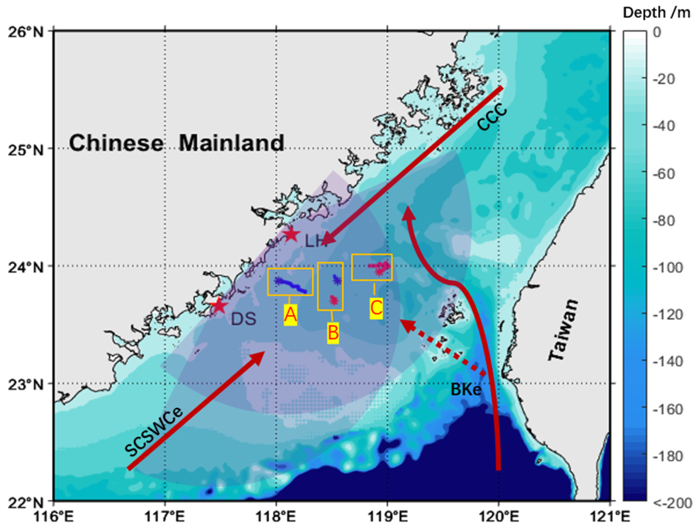
The Taiwan Strait, as a channel for maritime transportation and exchange between the South and East China Seas [21,22], is bordered by Chinese Taipei to the east and mainland China to the west. The average depth of the strait is relatively shallow, approximately 60 m [23]. It runs in a northeast–southwest direction, with the southern part being wider and the northern part narrower. Mountain ranges or hills run through both sides of the strait from north to south. The typical funneling effect in this narrow passage causes winds to gather, resulting in strong winds and waves, as well as fast currents in this region. The currents are complex, including the extension of the South China Sea Warm Current towards the northeast (SCSWCe), the southward Zhejiang–Fujian coastal current (CCC), and the northward branch of the Kuroshio current extending into the Penghu Strait on the eastern side of the strait (BKe) [24]. These complex topography and currents contribute to the relatively frequent occurrence of eddy activities in the Taiwan Strait.
In previous studies, researchers successfully captured several eddies through targeted on-site detection plans in the Taiwan Strait area [25,26]. However, due to the limited detection range, the regional characteristics of eddies cannot be obtained. Subsequently, with the development of high-resolution-satellite remote-sensing technology and the ocean numerical simulation results, people have a deeper understanding of the dynamic characteristics, spatio-temporal distribution, and transport properties of eddies [9,27,28,29,30]. However, the spatial and temporal resolution of Sea Level Anomaly (SLA) obtained by satellite altimeters is limited, making it difficult to apply them to the detection of coastal circulation and submesoscale eddies with radii smaller than 30 km [31,32,33]. In this aspect, high-frequency radar (HFR) stands out with its higher spatial and temporal resolution and relatively lower cost, becoming another widely used technology after satellite altimeters [34,35,36,37]. In the southwestern region of the Taiwan Strait, HFR technology has been applied to study the characteristics of surface currents [38,39,40], but its application in the analysis of submesoscale eddies is seldom, mainly focusing on the comparison and improvement of detection algorithms for eddies [41,42,43]. Among those, Lai et al. compared different algorithms in the application of compact HFR data and derived basic statistical characteristics of local eddies [41]. In this study, three cases were analyzed to show the characteristics and dynamic features of eddies in the southwestern region of the Taiwan Strait by using the data obtained by high-frequency surface-wave radars (HFSWRs) with an antenna array.
The automatic algorithm for eddy detection Is an essential part of the analysis. Depending on the types of data (Lagrangian data or Eulerian data), corresponding detection algorithms are selected [44]. Lagrangian data refer to the tracks of water parcels or particles, while Eulerian data denote snapshot data at a specific moment. The data acquired by HFRs obviously belong to the latter. Currently, detection algorithms for Eulerian data can be classified into three categories: the physics-based method, geometry-based method, and hybrid method, combining physics parameters and geometric features [45]. The first category needs to compare specific physical parameters with pre-set thresholds. For example, the most widely used Okubo–Weiss (OW) method includes the parameter OW (), where represents the shearing deformation rate, represents the stretching deformation rate, and represents the relative vorticity [46,47]. Methods based on geometric criteria primarily include the Winding-Angle (WA) and Vector Geometry (VG) methods. The WA method identifies eddies using closed curves [43], while the VG method determines the centers and boundaries based on four constraints related to the eddies [45]. Additionally, hybrid algorithms based on physical parameters and geometric features combine specific physical parameter methods with geometric methods. For example, eddies are detected by using the local extrema of sea surface height anomalies (SSHA) as potential eddies centers and combining them with geometric features of the enclosed current field around the potential eddies [9,27,48]. In recent years, with the rise of deep learning, researchers have also started to apply it to eddies detection [49,50]. Lai applied both the VG and WA methods to the detection of eddies in HFRs data, and the results showed that there was not a significant difference in the ability to identify eddies between the two methods [41]. Due to its flexibility, the VG algorithm has been widely applied to submesoscale eddy detections and found to satisfy the minimum criteria for both SDR and EDR [45,51]. Therefore, the VG method is selected in this study.
The article is structured as follows: Section 2 introduces the data and methods, including the HFSWR dataset, parameters to describe the characteristics of eddies, and the VG method. Section 3 shows the results of the analysis, covering three cases and regional statistical characteristics. The case analysis focuses on the temporal evolution of eddy features, while the statistical analysis includes the census and motion of eddies. Section 4 further discusses the dynamic characteristics of eddies, and the conclusions are provided in Section 5.
2. Data and Methods
2.1. Data
The experimental data applied here are the results of joint detection of ocean surface currents of the Taiwan Strait by using two HFSWRs with array antennas developed by Wuhan University (Wuhan, China) [52,53,54,55]. The data were collected from 29 January to 26 March 2013, covering a spatial range of 21.9°–24.5°N and 117.2°–120°E. The two radars were deployed at Dongshan (23.6575°N, 117.4863°E) and Longhai (24.2674°N, 118.1353°E), respectively, with a distance of approximately 90 km. The maximum detection range of each radar was about 200 km, and the angular resolution for radial flow was 1.5°. The beam coverage angle for the Dongshan station was 165°, while for the Longhai station, it was 155° (Figure 1). Both radars utilized a three-element Yagi-Uda antenna and an array of eight antennas for transmission and reception [39]. During the experiment, a frequency-modulated interrupted continuous wave signal was employed to reduce the co-frequency interference. The operating frequencies were selected within the range of 7.5–8.5 MHz and were unequal for the two radars. The data of vector currents were spatially interpolated by an inverse distance weighted during vector synthesis [56]. Finally, the data of vector flows had a temporal resolution of 10 minutes and a spatial resolution of 2.5 km, covering a time span of 57 days. To control the quality of data, the processing method offered by [40] was adopted.
2.2. Methods of Eddy Detection and Tracking
The Vector Geometry (VG) method is employed in detecting an eddy by sequentially determining its center and its boundary [45]. The VG method set four constraints to determine the center of an eddy: (1) the meridional (north–south) velocity component u changes sign on either side of the center, with increasing magnitude away from the center; (2) the zonal (east–west) velocity component v changes sign on either side of the center, with increasing magnitude away from the center; (3) the velocity at the center should be minimal; and (4) the rotation direction of the velocity vectors near the approximate center point should remain consistent. To quantify these constraints, two parameters, a and b, are defined. Parameter a determines the minimum range for detectable eddies, while parameter b determines the region of the local minimum velocity (in terms of spatial grid points of the data). Once the center is determined, the outermost closed contour surrounding is considered as the boundary of the eddy. The efficiency of this algorithm is evaluated by the Success Detection Rate (SDR) and Error Detection Rate (EDR) [48], which are defined as follows:
where is the number of real eddies detected by the algorithm. is the number of eddies detected by the algorithm which is inconsistent with the reality. is the total number of true eddies. The number of eddies mentioned here indicates the quantity of eddy centers detected by analyzing surface current maps.
A sensitivity testing of a and b is conducted to test the performance of the algorithm on applying it to the data of HFSWRs. The range of a is set to be [2,4] and that of b is [1,3], respectively [45,57]. One hundred randomly selected vector current maps were used to calculate SDR and EDR from Equations (1) and (2) for different combinations of a and b. The number of eddies obtained through the manual detection of the velocity vector field was given to , the true number of eddies. The number of eddies detected by the algorithm and the corresponding SDR and EDR values for each parameter combination are shown in Table 1. From the table, it can be observed that all combinations of EDR are within the specified limit (<20%). SDR is almost always less than 80%, which is the lower limit set by [48] for eddies’ automatic detection, with the exception of only when a = 3 and b = 1. On this occasion, we set a = 3 and b = 1 in the subsequent eddy detection. Furthermore, the results indicate that for a given value of a, SDR is negatively correlated with b. Considering that the search range for the minimum velocity point is determined by parameter b, when b is too large, only large eddies can be detected [45], resulting in a decrease in SDR.
After completing the detection of centers in all time intervals, the track is determined by tracing the positions of centers consecutively [45]. The motion of an eddy is influenced by the advection of the local flow field, and the range of the search area can be estimated by multiplying the average background velocity of current by the sample time. Considering that the sample time is 10 min and the average velocity at that time period is about 44.2 cm/s, a searching radius of three grids is then adopted taking into account the possibility that the actual eddy centers may be located in the edge region of the grid. In addition, if no associated eddy is detected at the next time, the search is performed by expanding the radius by 1.5 times. If a new center is found, the track is connected from time t. If not, the tracking is terminated. It should be noted that if multiple eddies of the same polarity are detected in the next time step, the one which is closest to that at the previous time step is selected.
2.3. Specific Eddy Attributes Determination
Relative vorticity (), divergence (), shearing deformation rate (), stretching deformation rate (), strain rate (), and energy intensity () are calculated to study the characteristics of the eddies obtained. They are defined as follows:
where and are the eastern () and southern () speeds in local rectangular coordinate, respectively, derived from the HFSWRs. The area of the eddy (s) is given by the area of a circle of radius R. The radius R is another important parameter to measure the eddy, and it is calculated based on the maximum closed streamline around the center. There are generally two methods for calculating the radius in practice: one is to take the average distance between the center and the boundary obtained by the algorithm as the eddy’s radius [41], and the other is to consider the eddy as a circle and obtain the radius using the area enclosed by the outermost closed curve [57]. By comparison, it is found that the average deviation of radii calculated by these two methods is only 0.31 km, and there is no difference in the distribution of the radii in this study. As a consequence, we only applied the first method in the subsequent work to calculate the radii of eddies.
3. Results
A total of 1152 tracks of eddies are detected from the data of HFSWRs by using the method mentioned in Section 2. However, in order to exclude the noise in the measurements, those eddies that appear in only one dataset are not be included in subsequent analyses. Therefore, only 414 eddies were involved in the analysis, out of which, 253 were cyclonic and 161 were anticyclonic eddies. The number of cyclonic eddies is approximately one and a half times that of the other. Three cases are selected as examples to show the details of the eddies.
3.1. Case Studies
3.1.1. Case A
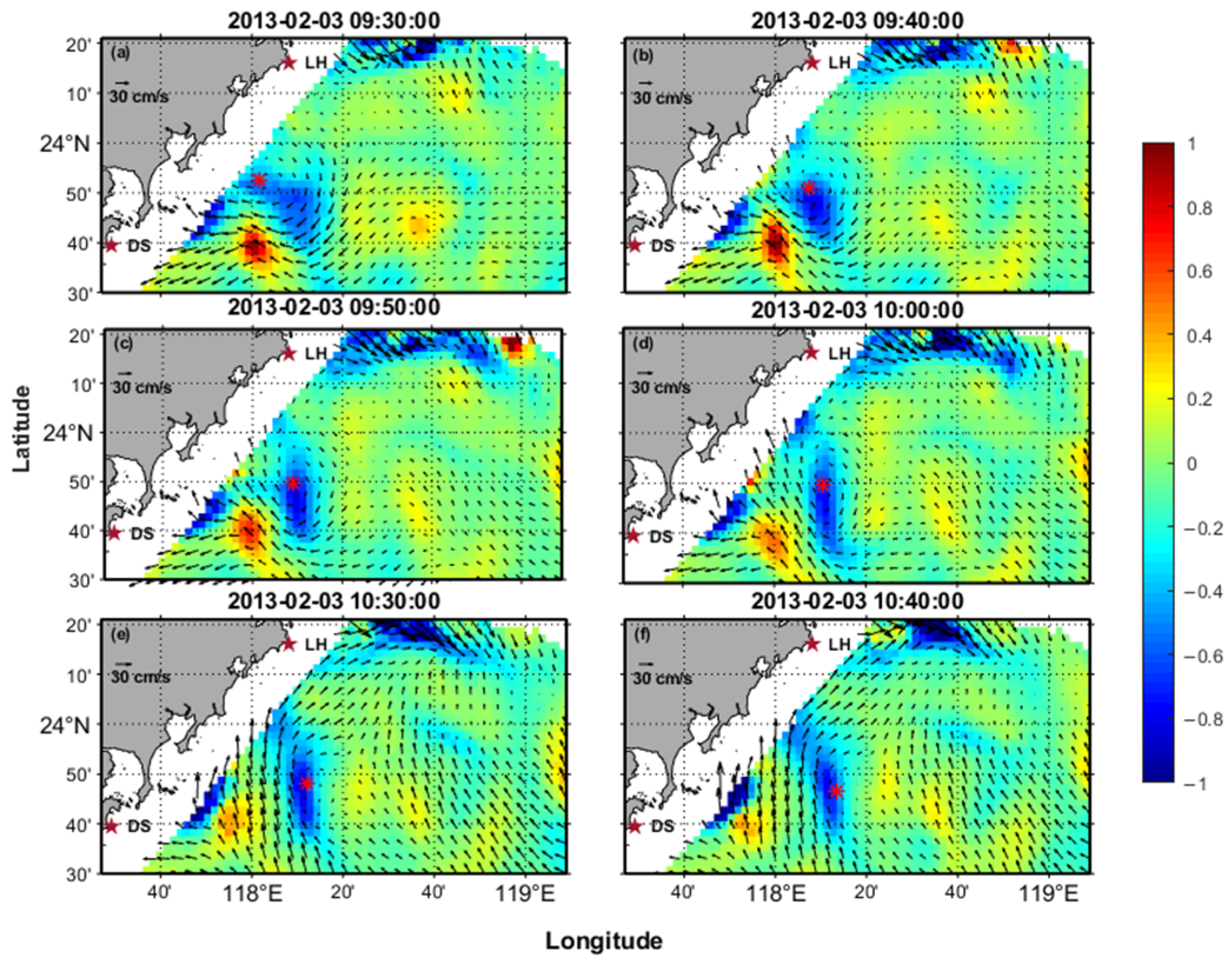
Case A is an anticyclonic eddy that occurred at around 9:30 on 3 February 2013, with a duration of approximately 70 minutes. It is worth noting that all times that appear in this paper are in Beijing time (UTC+8). Figure 2 shows the velocity of the surface current by black arrows, and the value of relative vorticity normalized by the Coriolis parameter () was indicated by the colormap. The black arrows show that an anticyclonic eddy was forming from 9:30 to 10:00 in the current and then deformed at about 10:40. The red star in each panel indicates the eddy center at that time, and according to the calculation, the center of the eddy moved about 27.8 km to the southeast during its lifetime. Figure 1 shows that eddy A originated at a shoal with a water depth of ~20.4 m, and it moved over this shoal for most of its life, then dissipated just after entering a deeper area with a water depth of ~44.3 m. Figure 2 shows that is negative in the eddy region for its clockwise flow. The magnitude of near the eddy center increases with time before the last panel. The contour shape of stretches in the south–north direction with time.
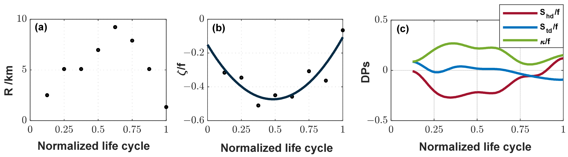
Figure 2a shows that the currents are curled, and the streamline is almost closed to form an eddy at that moment. More streamlines are closed, and the eddy shape becomes more like a circle with time as shown in Figure 2b–d. The radius increases to ~9.2 km in this period as shown in Figure 3a. After that, the eddy is stretched in the south–north direction as shown in Figure 2e,f. It also shows that the current speed in the eddy’s east part slowed down, while that close to the mainland increased with the eddy moving southeast in the last two panels. The eddy’s radius shortened sharply at the last several moments as shown in Figure 3a.
The magnitude of relative vorticity at the center of the anticyclonic eddy increased first and then decreased (Figure 3b). Figure 2 shows that the eddy tended to elongate during its movement, which is also confirmed in Figure 3c. In the first 7/8 stages of the life cycle, , which generally indicated compression in the northeast–southwest direction and stretching in the northwest–southeast direction. During this process, hovered around zero and gradually developed into a value less than it, implying a tendency of east–west compression and south–north stretching, and gradually exhibited this characteristic. In the last 1/8 stage, and , indicating that the eddy continued to stretch in the north–south and compress in the east–west direction, with more obvious stretching in the northeast–southwest direction. In the Okubo–Weiss method, the parameter is an important indicator to measure the dominance between relative vorticity and horizontal strain in local dynamic features [43,44]. When the value is greater than 0, local horizontal strain dominates over relative vorticity; when the value is less than 0, the relative vorticity plays a more important role in local dynamic features. In this study, this parameter is also included in the measurement of eddies’ characteristics. Through calculations, it is found that the values of near the centers were negative at all times, with a mean value of , gradually approaching 0 as it moved away from the center of the eddy. This indicated that the relative vorticity played a major role in the local dynamic features of this eddy and its influence weakened as it extended outward from the center.
3.1.2. Case B
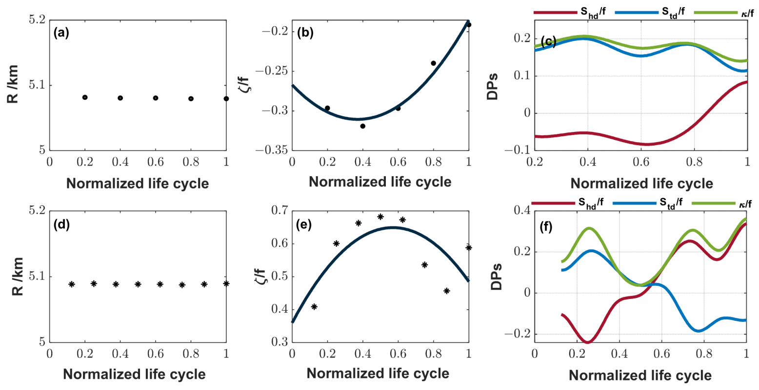
In this case, we selected two eddies of opposite polarity that were generated and disappeared almost simultaneously in adjacent regions for demonstration. The yellow box marked B in Figure 1 is the active area of the two eddies in this case. The cyclonic eddy was generated about 10 minutes earlier than the anticyclonic one. After about an hour, the cyclonic eddy disappeared, while the other one had faded away about twenty minutes before it (Figure 4). Similar to the previous case, the two eddies’ value of varied between and , both belonging to the submesoscale process. Their average size was similar, with a radius of about 5.1 km. The positions of the two eddies hardly changed during their lifecycles (Figure 1), with only a slight northward shift, and the distance was almost the same, about 6.1 km. According to the local vector current maps, it can be roughly seen that the anticyclonic eddy was generated owing to the interaction between the northward current of the cyclonic eddy in the south and the current from the left. As times passed, the velocity of the leftward current gradually diminished, unable to counterbalance the upward flowing current, resulting in the disappearance of the anticyclonic eddy. Moreover, we also studied the temporal evolution of two eddies’ characteristics in this case (Figure 5). As far as the temporal variation of relative vorticity is concerned, it is apparent that both are similar to the previous case (Figure 5b,e), with their absolute values initially increasing and then decreasing. Figure 5a,d show that there was almost no change in the radii of the two eddies, indicating that the structures of the eddies remained relatively stable throughout their lifecycles, with no significant signs of growth after their generation. Figure 5c,f illustrate the deformation parameters of the two eddies. By comparison, the shape of the anticyclonic eddy remained relatively stable throughout the entire process, with a slight fluctuation in the normalized strain rate () around 0.18. On the other hand, the cyclonic eddy approached a circular shape at the intermediate moment and became more dispersed at the edge moment. Additionally, it is found that the parameter near the centers of the two eddies are both negative, with mean value of for the anticyclonic eddy and for the other. Consequently, in this case, the relative vorticity still played a leading role in the local dynamic characteristics, but compared to the cyclonic eddy, it was not prominent in the anticyclonic one.
3.1.3. Case C
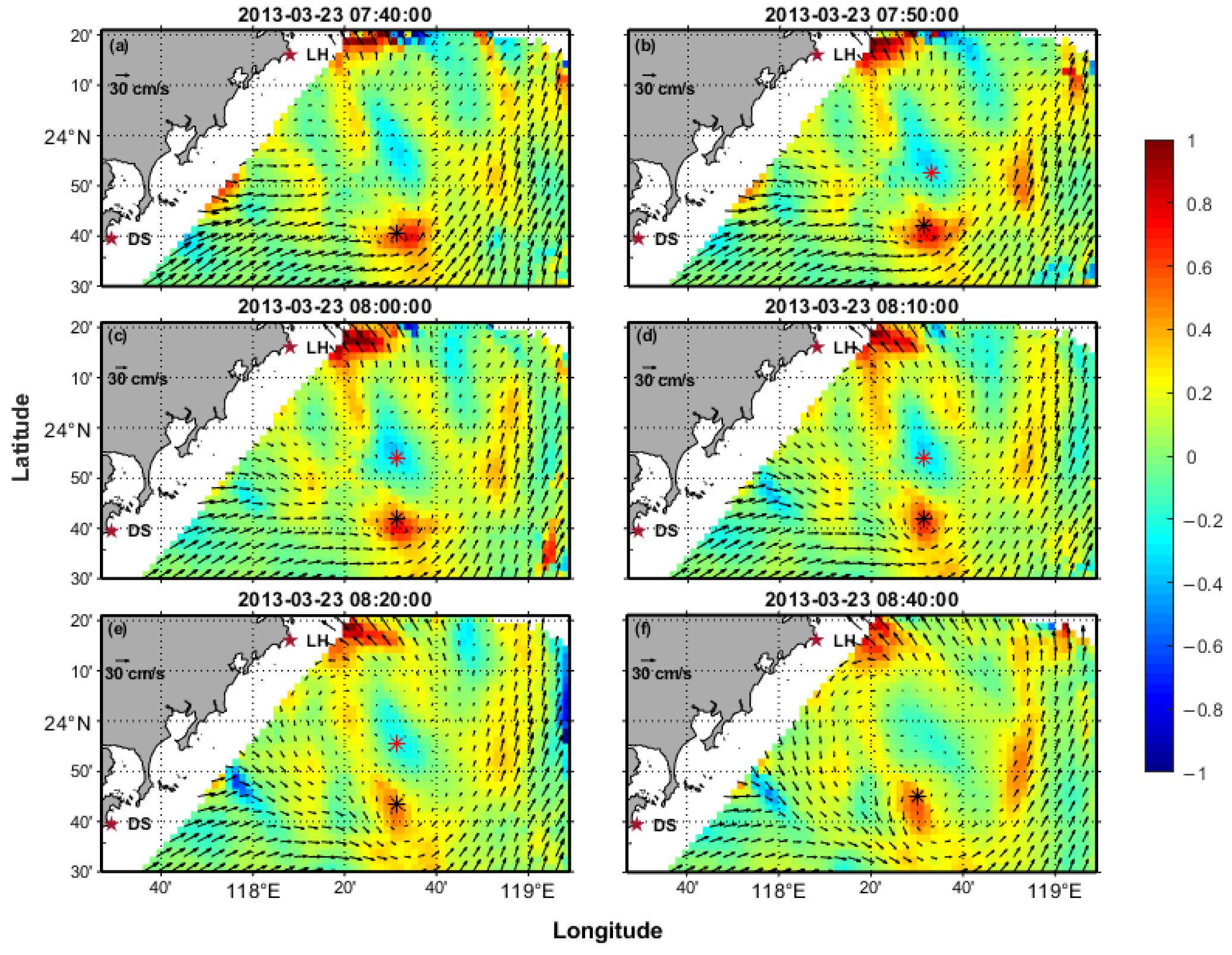
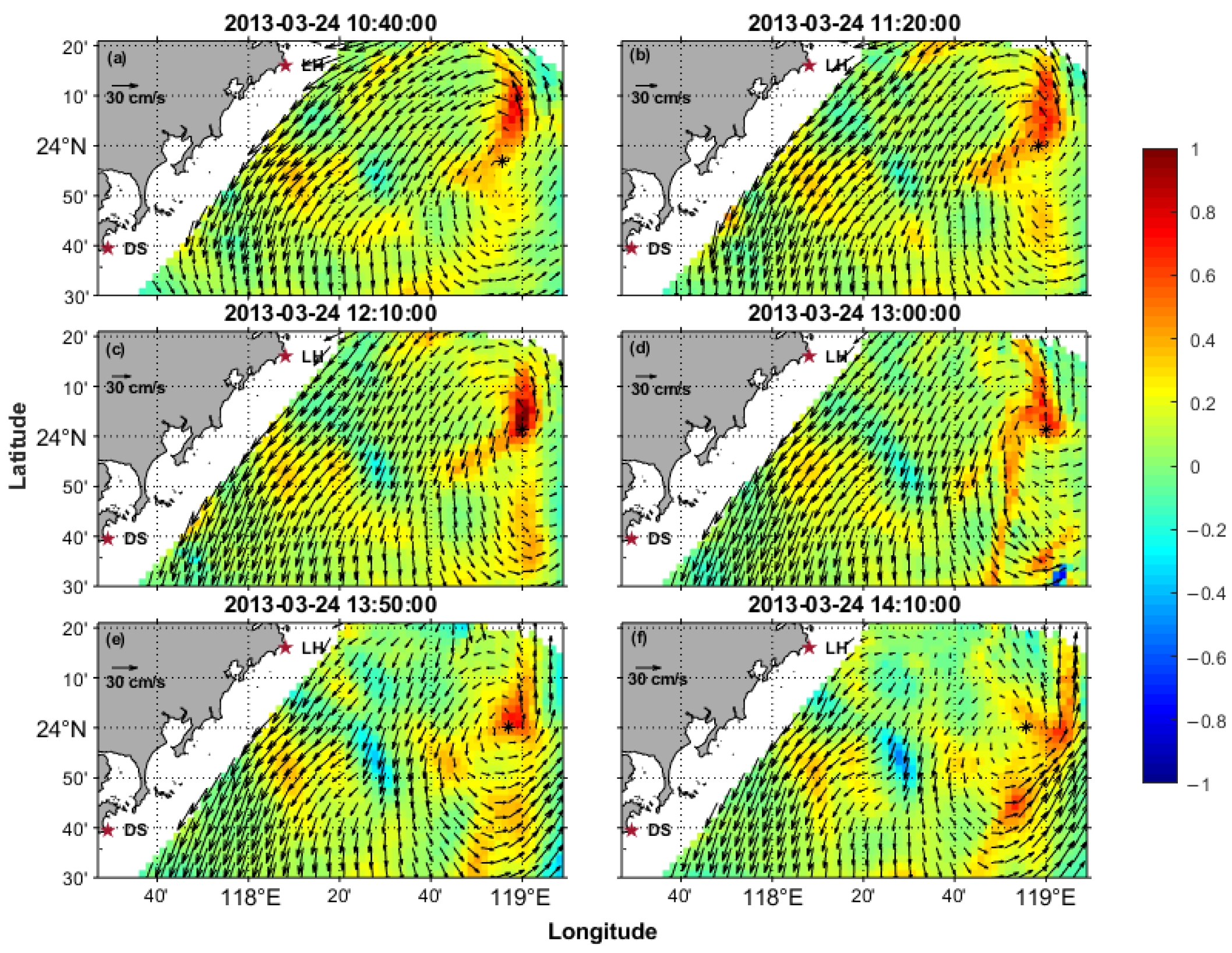
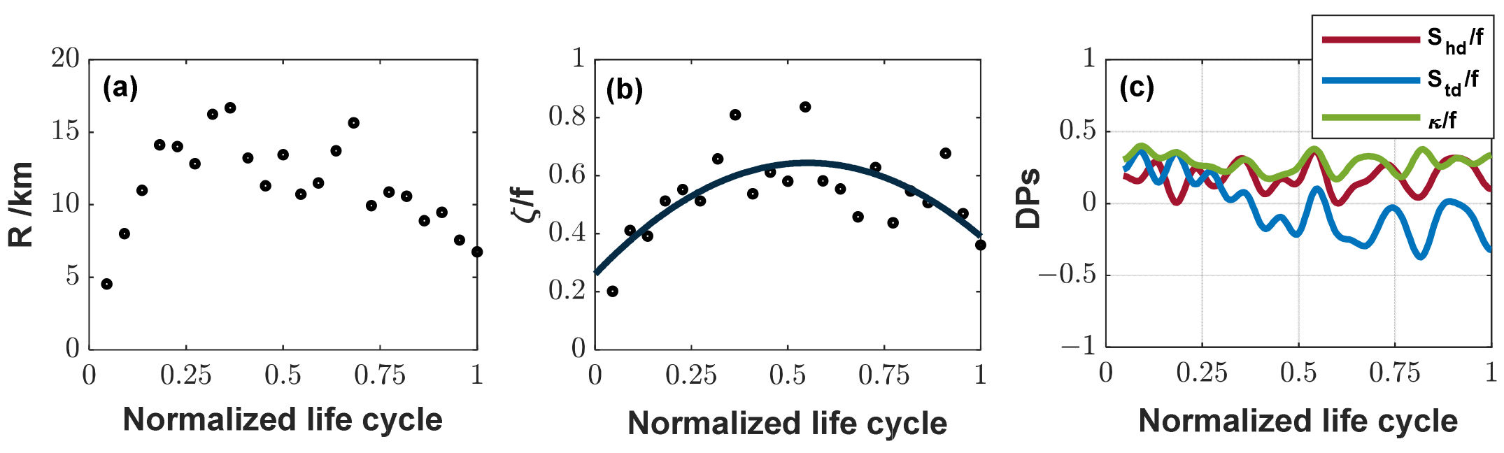
This is the final case in which we chose a cyclonic eddy with the longest duration. It occurred on 24 March 2013, at 10:40, with an average radius of 11.1 km and a lifecycle of approximately 3.5 h. Figure 6 exhibits the maps of the vector current at six different moments, with Figure 6a and f showing the first and last observations of the complete structure, respectively. The eddy originated in an area with a water depth of approximately 55 m. It initially moved in the northeast direction, then meandered westward before eventually dissipating in an area approximately 11.6 km away from its birthplace (Figure 1). The temporal variations in size and relative vorticity were similar, reaching a maximum at around the midpoint of its lifespan (Figure 7a,b), which was consistent with the results of the first case. Taking the morphological changes during the movement of the eddy into account, as shown in Figure 7c, remained positive throughout the entire process, indicating elongation in the northeast–southwest direction and compression in the northwest–southeast direction. On the other hand, presented a fluctuating decline and ultimately became negative, making clear a gradual compression in the east–west direction and stretching in the south–north direction. Additionally, based on computation, the parameter near the center of this eddy remained negative with a mean value of −2.2 × suggesting that the local dynamic characteristic around the center was dominated by relative vorticity, which is the same as the results of the above two cases.
In this section, the morphological changes of eddies were visually displayed through three case studies, and the temporal evolution of their characteristic parameters was analyzed. Based on the analysis of the aforementioned cases, we can find some common features among these cases, such as the temporal evolution of the relative vorticity and the variation in parameter from the eddies center to the periphery. In order to acquire the regional characteristics of eddies in a more systematic and comprehensive manner, we conducted a basic feature survey in Section 3.2, including the spatial distribution, statistical analysis of size and lifespan, the distribution of relative vorticity, and the motion of eddies.
3.2. Statistical Characteristics
3.2.1. Eddy Distribution
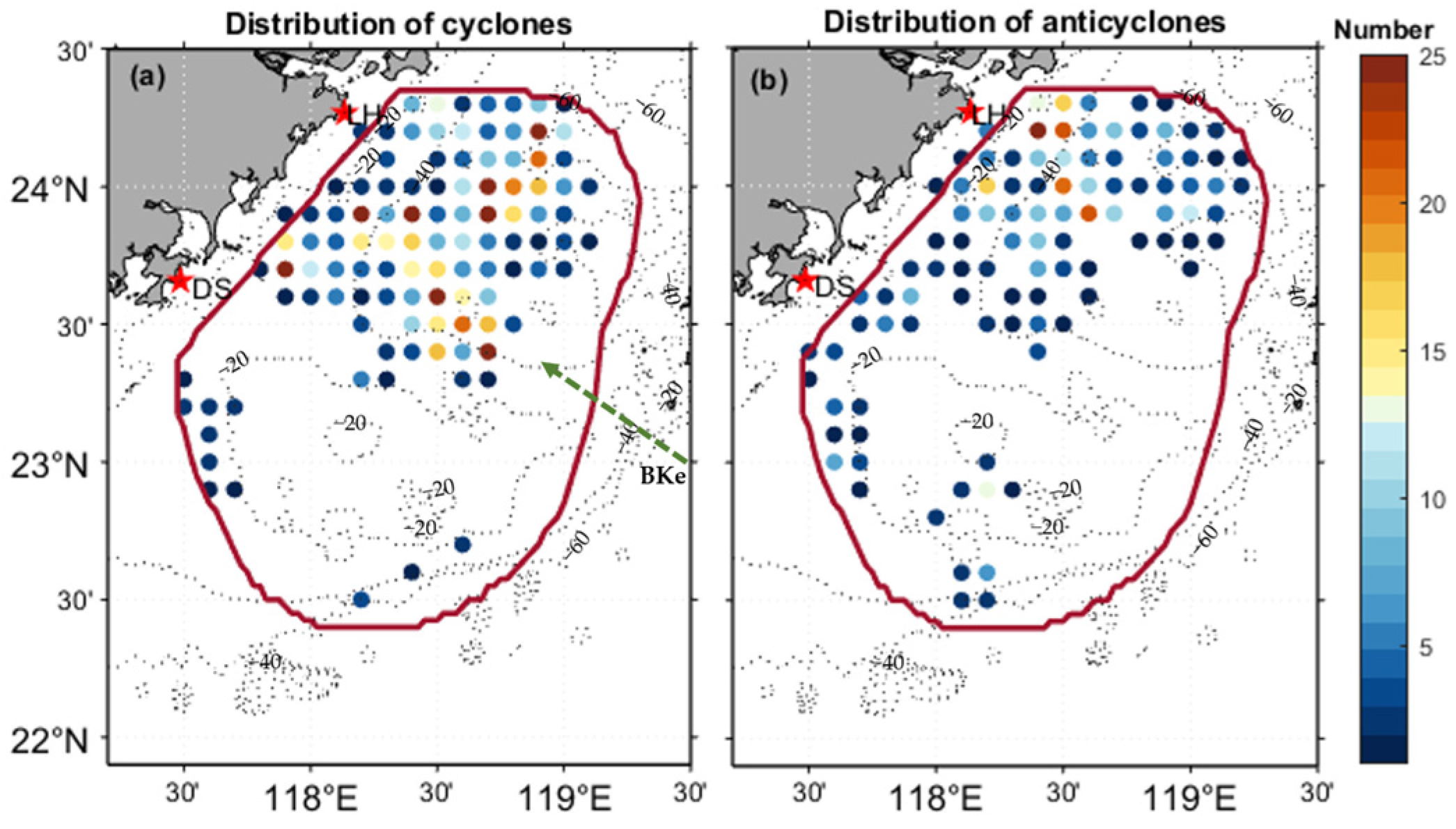
Figure 8 shows that eddies generally occur north of Taiwan Strait Shoal. The cyclonic eddies tend to gather near the 40 m and 60 m isobaths, while anticyclonic eddies occur most frequently in the northwest of the detection region. Combined with Figure 1, it can be found that the frequent occurrence of cyclonic eddies is located in the intersection area of the three major currents SCSWCe, CCC, and BKe. The green arrow in Figure 8a simply indicates the direction of the BKe, and the number of cyclonic eddies in this direction is significantly higher than that in other regions. However, the number of eddies in Taiwan shoals is small, and the occasional eddies are mainly distributed near the water depth contour, which indicates that the generation of eddies in this area is affected by the topography. In addition, eddies in the west side of the shoal are denser than those in other parts of the area, which may also be related to the extension of the South China Sea warm current flowing through the area.
3.2.2. Radius
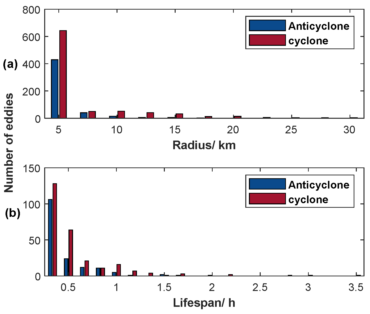
Figure 9a shows a similar distribution of the radius for anticyclonic and cyclonic eddies, concentrated in the range of 5–7.5 km. The average radius of total eddies is 6.5 km, with an average radius of 5.7 km for anticyclonic and 7.0 km for cyclonic eddies. It was found that anticyclonic eddies with a radius exceeding 10 km accounted for only 4.0%, and the maximum of it was 17.5 km, while the other type could reach 27.8 km. Additionally, it is worth noting that the VG method is generally not good at capturing the size of eddies [41]. Therefore, the results of the radius may not be accurate.
3.2.3. Lifespan
Figure 9b shows the distribution of eddies’ lifespan. Similarly, the distribution of the two types also exhibited the same characteristics, with the number gradually decreasing as their lifespan increased. Furthermore, there were only eight eddies with a lifetime exceeding 90 min during the period of study, and only two of them were cyclonic eddies. The track of cyclonic eddies could last up to 3.5 h, and the other type merely sustained 3 h at most. Overall, eddies captured by the high-frequency radar in the study area generally had a short lifespan, and after excluding eddies seen only once, the average lifetime of the remaining is 0.88 h. This is consistent with the conclusion (~0.7 h) offered by [41], considering that it did not exclude eddies that survived only one dataset.
3.2.4. Vorticity
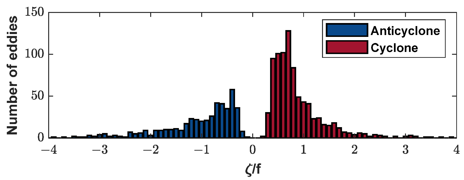
Theoretically, the maximum relative vorticity is at the center of the eddy. Here, we take the maximum value as the relative vorticity of the eddy and divide it by the local Coriolis force coefficient . Figure 10 shows the histogram of the relative vorticity normalized by , with anticyclonic eddies on the left and cyclonic eddies on the right. It can be seen that the distributions of both types of eddies were skewed. The value of varied with the quasi-geostrophic and submesoscale . The peak range of relative vorticity of anticyclonic eddies (0.3–0.4) was lower than that of cyclonic ones (0.6–0.7). However, the absolute value of anticyclonic eddies’ average relative vorticity (~1.1) was slightly higher than that of cyclonic eddies (~0.9).
3.2.5. Motion of Eddies
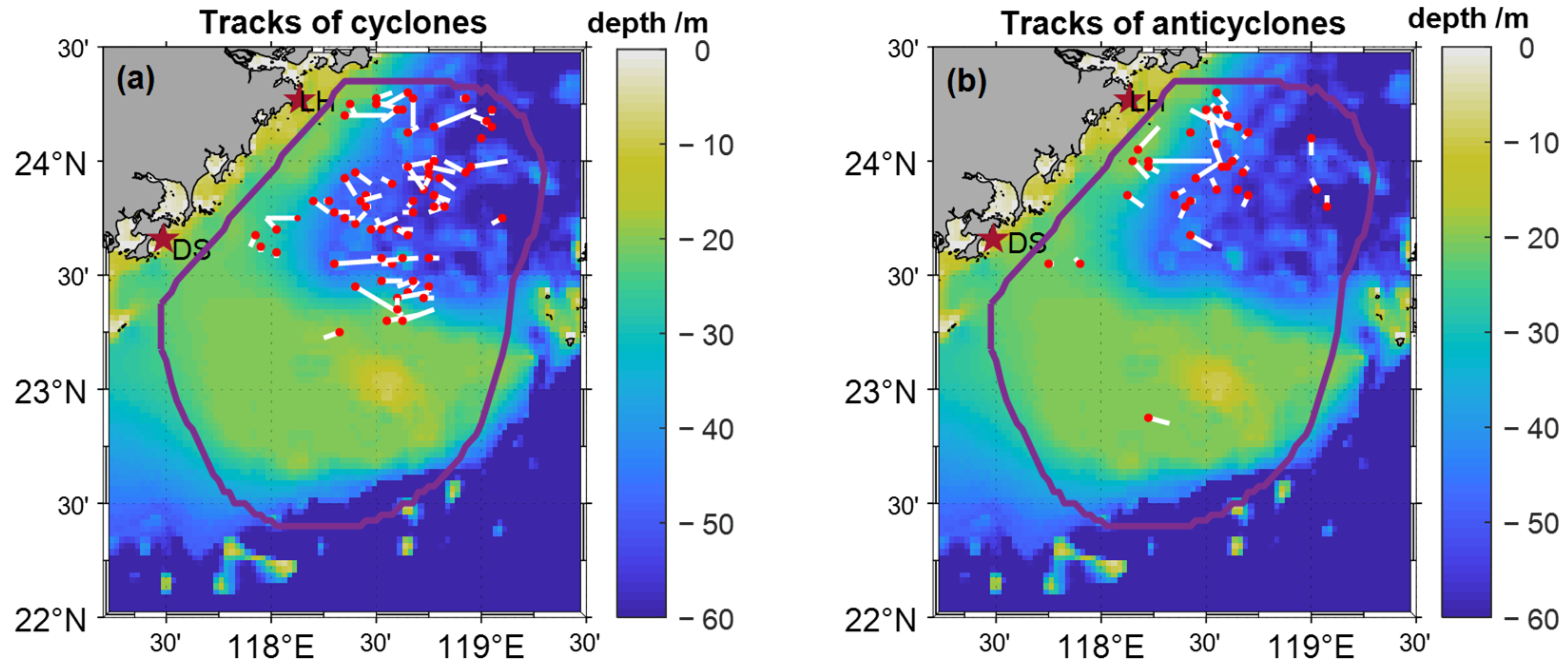
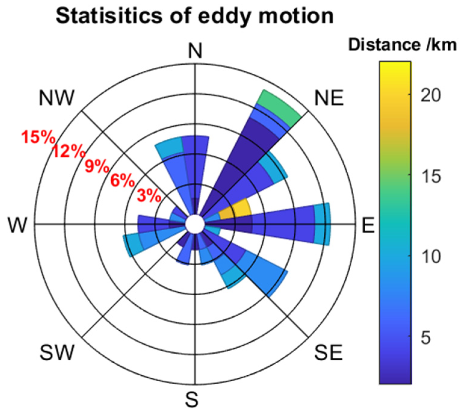
In order to understand the characteristics of propagation, we further investigated the movement of eddies with the lifecycle exceeding half an hour (anticyclonic: 68, cyclonic: 34). The distances of eddies’ movement were generally not far in our study area, and cyclonic eddies showed more obvious eastward and northeastward motion characteristics (Figure 11a), while the movement of anticyclonic eddies appeared to be more random without a clear advantage in direction (Figure 11b). Figure 12 shows the statistics of eddies’ motion including their directions and distance. The polar coordinate system is divided into 20 directions (the north is positioned at 0°, and the degree increments in a clockwise direction), and the length represents the frequency of eddies moving towards a certain direction. The longest part in Figure 12 represents the highest proportion of eddies moving in the direction of north by east 27 to 45 degrees, reaching up to 14.1%. Additionally, the color bar in each part represents the distance of movement in that direction. Therefore, the track of eddies moving in the direction of north by east 27 to 45 degrees were distributed between 4 and 15 km, with the highest proportion being between 4 and 6 km. Figure 12 shows the overall preference for eddies to move towards the east after their generation, with a prominent eastward and northeastward movement, consistent with the features shown in Figure 11. The relatively dark blue in the image also indicates that despite some directional preferences, the majority of eddies detected in this region have little change in positions during their lifetime. Interestingly, eddies with tracks longer than 20 km showed little deviation in their directions of motion, all located within the range of north by east 63 to 81 degrees.
3.2.6. Evolution of Eddies
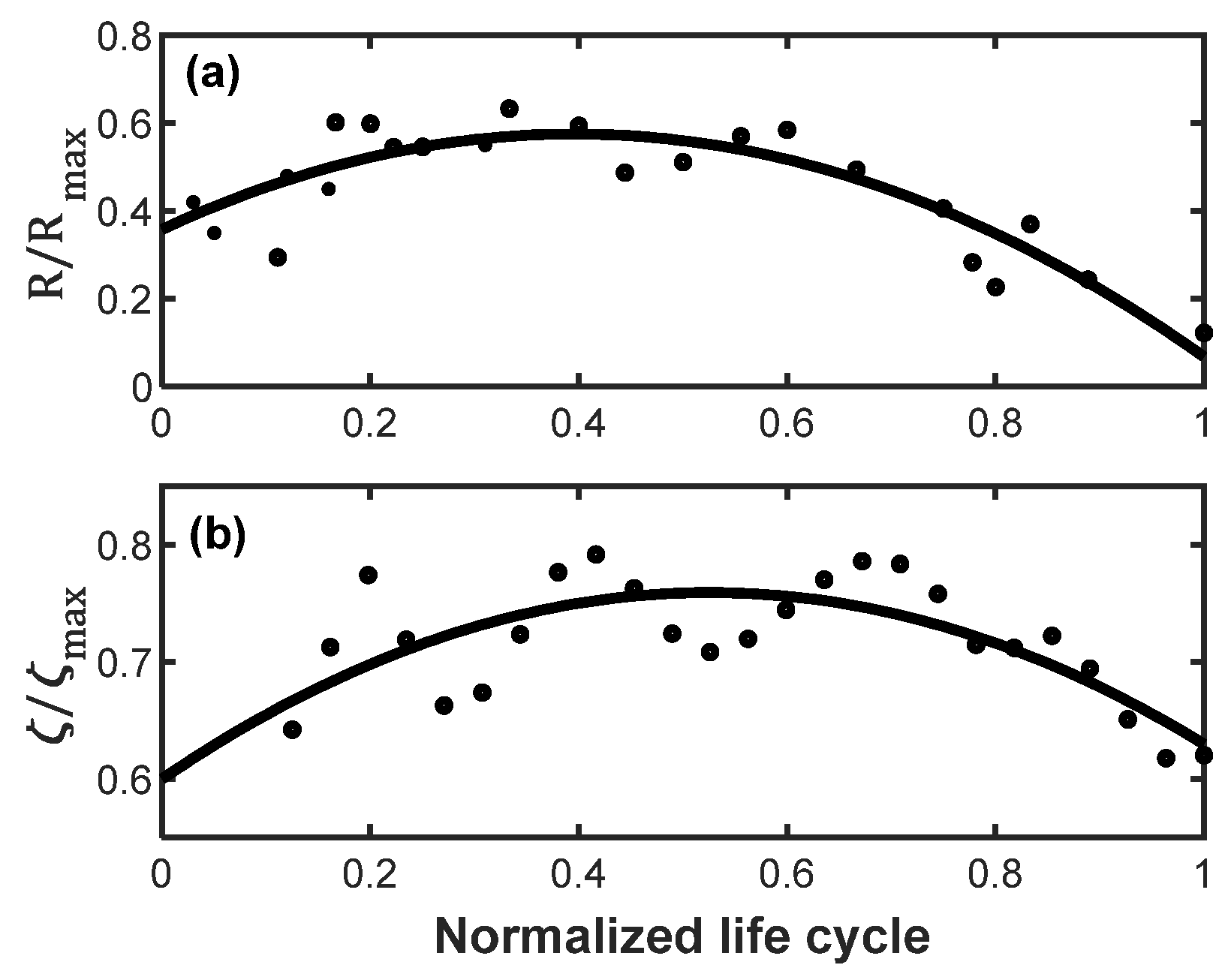
In the case studies in Section 3.1, we found certain similarities between the radii of eddies and the temporal evolution of relative vorticity. Therefore, we studied the characteristics of evolution using the 102 eddies with a lifetime exceeding half an hour mentioned earlier. We divided the life stage by the lifetime of the eddies to obtain a standardized lifecycle and normalized the radius and relative vorticity by dividing them by their respective maximum values within their lifetime (Figure 13). The black dots represent the actual values, while the solid lines are the fitted results. The root-mean-square errors were calculated to be 0.14 and 0.17, respectively. According to the fitting results, the radius underwent two main changes. In the first 2/5 of the period, it showed an increasing trend on the whole, with eddies continuously growing. After that, eddies started to weaken, and the rate of decrease in radius was slightly faster than that of the increase (Figure 13a). As for the relative vorticity, it exhibited a similar change to the radius, and the maximum value of the fitting results occurred in the middle (Figure 13b). However, it is worth noting that the actual values of the relative vorticity seemed to have a periodic characteristic. It reached a local maximum in the first 1/5 stage, and then achieved local maxima again at 2/5 and 2/3, followed by a fluctuating decline. It is apparent that the magnitudes of the local extremum values at these three moments were similar, and there is no advantage in the overall maximum value throughout the process.
4. Discussion
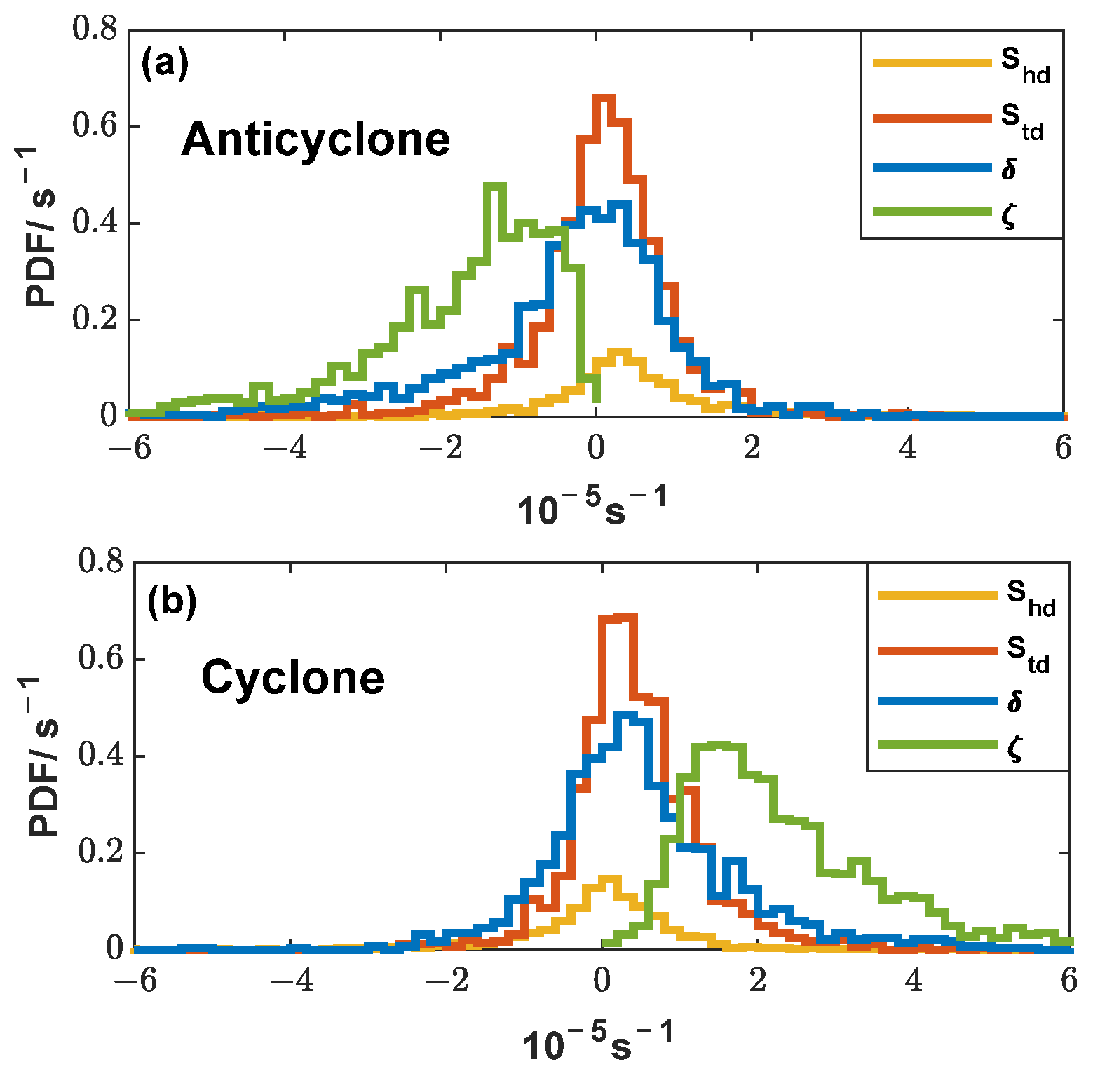
In the previous section, we analyzed the basic statistical characteristics of eddies in the study area. In this section, we will focus on the dynamic properties of eddies based on the probability distribution of dynamic parameters. Figure 14 shows the probability density functions of the kinematic parameters of eddies. Through calculations, the stretching deformation rate and shearing deformation rate of anticyclonic eddies follow the normal distribution with mean values of and , respectively. Similarly, the two deformation rates of cyclonic eddies also follow the normal distribution of mean and , respectively. The overall strain rates of both types of eddies were similar, with means of and , respectively. These results indicated that regardless of the type of eddies, their shapes kept changing during motion so that it was difficult to maintain the original structures. However, the deformation patterns between them were different. The negative mean of anticyclonic eddies implies that they tended to compress in the northeast–southwest direction and extended in the northwest–southeast direction, while the positive suggests an extension in the east–west direction and compression in the north–south direction. In comparison, cyclonic eddies mainly exhibited compression in the east–west direction and extension in the north–south direction. Additionally, the divergence of these two types (anticyclonic: ; cyclonic: ) differed by one to two orders of magnitude from the vorticity values (anticyclonic: ; cyclonic: ), indicating strong shear in the eddies. The smaller divergence of cyclonic eddies suggests that there was less loss of water during evolution, implying that cyclonic eddies were relatively more stable compared to anticyclonic ones. This is consistent with the conclusion mentioned in the previous section that cyclonic eddies generally last longer.
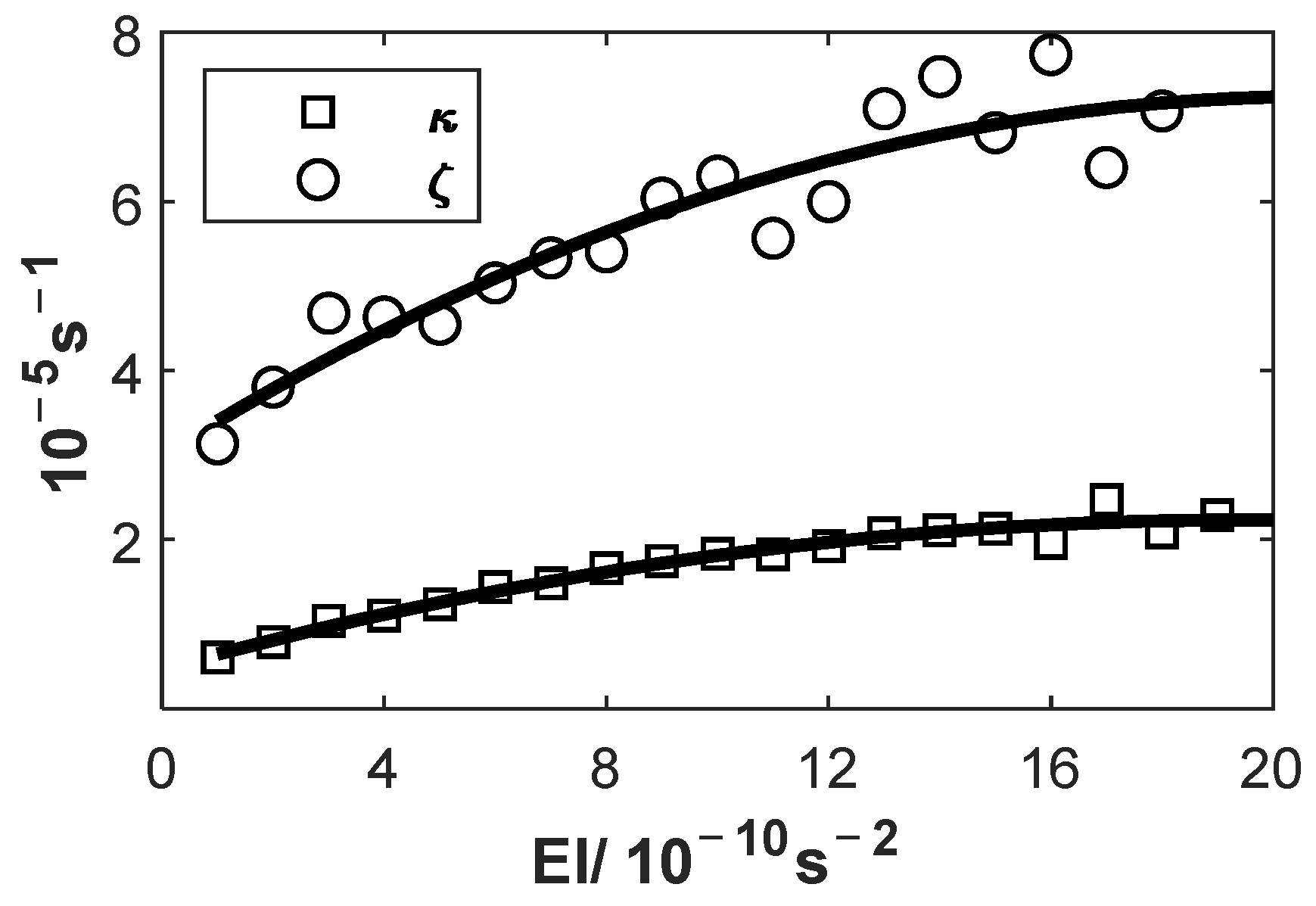
Previous studies on the relationship between characteristic parameters have indicated some correlations among the size of eddies, strain rate, and EI [41,58]. Building upon this assumption, the associations among the relative vorticity , the average strain rate and energy intensity EI are displayed in the Figure 15. The two solid black lines are quadratic fitting lines, with root-mean-square errors of 0.41 and 0.09, respectively. The fitting results suggest that and both had a quadratic relationship with EI, and as EI increased, the value of and increased as well. It was found by [41] that smaller eddies tend to be more circular based on their study of the relationship between size and strain rate. However, the sizes of eddies detected in this study were relatively concentrated, and there was no clear corresponding relationship between them. Further data verification and theoretical derivation are needed to verify whether they have a certain association.
Due to the limited research materials and the complex behavior of coastal currents, it is difficult to understand the formation mechanism of eddies in this region. Nevertheless, the analysis of the eddies’ local characteristics reveals that the topography and the major currents flowing through this region may be related to their formation. Figure 8 shows a preference for eddies to occur north of the Taiwan Strait shoals, where according to Figure 1, three major currents intersect. It seems that the intersection of the China Coastal Current and the branch of Kuroshio’s extension is conducive to the formation of cyclones, and the relatively dense cyclones shewn in the upper right corner of Figure 8a support this deduction. In addition, the number of cyclones along the direction of the branch of Kuroshio’s extension indicated by the dotted arrows in Figure 1 is higher than that in surrounding areas, highlighting the impact of the Kuroshio in this region. The complex topography also affects the generation of eddies. In the shallow bank area where the number of eddies is quite small, almost all of them are distributed near the water depth contour with great variation. The interaction between ocean currents and undulating terrain generates eddies. However, since the water is shallow here, the bottom friction drag force leads to the short lifetime of the eddies which can be seen from the comparison between Figure 8 and Figure 11. The number of eddies with relatively long lifespan obviously decreases at the place where the depth of water is less than 40 m. It is worth noting that on the eastern side of Taiwan Island, which is close to our study area, the submesoscale island wake in the Kuroshio is being paid attention [59,60], which inspires us to think about the nature of the detected eddies. However, only the data of surface current are not enough to support the follow-up research, and the water system in the study area is relatively complex, so whether the eddies detected by us are wake vortices and which current dominates remain to be further studied.
5. Conclusions
This study is based on data obtained by the HFSWRs to analyze the characteristics of submesoscale eddies in the region of the southwest Taiwan Strait from cases on the whole. The automatic detection algorithm based on vector geometry was applied to HFSWR-derived surface current maps along the Fujian coast. A total of 414 tracks of reasonable eddies were detected within a period of nearly two months, including 161 anticyclonic and 253 cyclonic eddies. Eddies generally had a short duration, with the mean lifetime of 0.88 h, and only 102 eddies survived more than half an hour, of which there were exactly twice as many cyclones as anticyclones (anticyclonic eddies: 34; cyclonic eddies: 68). Both types of eddies were more frequently observed in the northern part of the study region with a latitude over 23.5°N, particularly those with a lifetime of over half an hour. In general, there were no significant differences in the distribution of size, lifespan, and relative vorticity between anticyclonic and cyclonic eddies. The radius was mainly concentrated between 5 and 7.5 km, with an average of approximately 6.5 km, and those with a radius of more than 10 km are almost all cyclones since anticyclones only account for 8.5%. Moreover, the value of varied within the quasi-geostrophic and submesoscale ranges, with the dominant value of 0.3–0.4 for anticyclones and 0.6–0.7 for cyclones. Eddies with a lifespan of over half an hour were concentrated in areas with a water depth of over 40 m and tended to move towards the east or northeast after generation, especially cyclonic eddies. On the whole, eddies travelled short distances, with an average distance of 6.1 km. Interestingly, eddies that moved more than 20 km are similar in their direction of motion with deviations of less than 18°. The normalized radius and vorticity of the eddies showed a periodic change in characteristic parameters during their lifespan. The shapes of the eddies were difficult to maintain during their movement, with anticyclonic eddies stretching in the east–west direction and compressing in the south–north direction, while cyclonic eddies displayed the opposite trend. However, the structure of cyclonic eddies was more stable. In addition, the relative vorticity and strain rate both had quadratic relationship with energy intensity.
In this study, a systematic statistical analysis of the submesoscale eddies in the southwest Taiwan Strait was completed. Due to HFSWRs’ high spatio-temporal resolution, a large number of submesoscale eddies were captured over a period of nearly two months. The research shows that the survival time of these vortices is generally short, and the birthplaces of the eddies with relatively long lifespans are more concentrated, and the movement direction in the life cycle has similar preferences, which also implies that the regional topography has a certain influence on the formation and development of the vortices. However, due to the limitation of the data used, the analysis of the seasonal variation of the vortices in this region cannot be completed in this paper. Subsequent work will aim to fill in this gap with a longer period of measured data. In addition, the relationship between the size of the eddies and the strain rate still needs further verification.
This paper shows the characteristics of submesoscale eddies in the southwest Taiwan Strait, and the results may provide insights for fishery prediction, oil spill and red tide diffusion monitoring, and submarine cable safety assessment. Furthermore, the study is an attempt to apply array HFSWRs to detect submesoscale eddies, and it proves that the array HFSWRs is feasible in the study and application of submesoscale dynamics which expands the application of the radar.
Author Contributions
Conceptualization, H.Z.; methodology, X.Y. and H.Z.; software, H.Z.; data curation, L.W.; formal analysis, H.Z., L.W. and Z.C.; writing—original draft preparation, H.Z.; writing—review and editing, H.Z., X.Y., Z.C. and L.W.; visualization, H.Z.; supervision, X.Y. and X.W.; project administration, X.Y. and X.W.; funding acquisition, X.Y. and X.W. All authors have read and agreed to the published version of the manuscript.
Funding
This work was supported in part by the Guangdong Province Key Field R&D Program, 2020B1111020005; in part by the Key R&D Program of Hubei Province, 2020BCA080.
Data Availability Statement
The data presented in this study can be found in the Scholars Portal Dataverse at https://doi.org/10.5683/SP2/QK4LGH (Wang et al., 2021 [40]).
Acknowledgments
The authors thank Changming Dong, who is currently with the Oceanic Modeling and Observation Laboratory, Nanjing University of Information Science and Technology, for his help in solving the confusion with the VG method.
Conflicts of Interest
The authors declare no conflicts of interest.
References
- Mcwilliams, J.C. The Vortices of Two-Dimensional Turbulence. J. Fluid Mech. 1990, 219, 361. [Google Scholar] [CrossRef]
- Doglioli, A.M.; Blanke, B.; Speich, S.; Lapeyre, G. Tracking Coherent Structures in a Regional Ocean Model with Wavelet Analysis: Application to Cape Basin Eddies. J. Geophys. Res. Ocean. 2007, 112. [Google Scholar] [CrossRef]
- Yang, Y.; Wang, D.; Wang, Q.; Zeng, L.; Xing, T.; He, Y.; Shu, Y.; Chen, J.; Wang, Y. Eddy-Induced Transport of Saline Kuroshio Water into the Northern South China Sea. JGR Ocean. 2019, 124, 6673–6687. [Google Scholar] [CrossRef]
- Bassin, C.J.; Washburn, L.; Brzezinski, M.; McPhee-Shaw, E. Sub-Mesoscale Coastal Eddies Observed by High Frequency Radar: A New Mechanism for Delivering Nutrients to Kelp Forests in the Southern California Bight: COASTAL EDDIES. Geophys. Res. Lett. 2005, 32. [Google Scholar] [CrossRef]
- Thomas, L.N.; Tandon, A.; Mahadevan, A. Submesoscale Processes and Dynamics. In Geophysical Monograph Series; Hecht, M.W., Hasumi, H., Eds.; American Geophysical Union: Washington, DC, USA, 2008; Volume 177, pp. 17–38. ISBN 978-0-87590-442-9. [Google Scholar]
- Wang, X.; Li, W.; Qi, Y.; Han, G. Heat, Salt and Volume Transports by Eddies in the Vicinity of the Luzon Strait. Deep Sea Res. Part I Oceanogr. Res. Pap. 2012, 61, 21–33. [Google Scholar] [CrossRef]
- Yang, Y.; Zeng, L.; Wang, Q. How Much Heat and Salt Are Transported into the South China Sea by Mesoscale Eddies? Earth’s Future 2021, 9, e2020EF001857. [Google Scholar] [CrossRef]
- Capet, X.; McWilliams, J.C.; Molemaker, M.J.; Shchepetkin, A.F. Mesoscale to Submesoscale Transition in the California Current System. Part I: Flow Structure, Eddy Flux, and Observational Tests. J. Phys. Oceanogr. 2008, 38, 29–43. [Google Scholar] [CrossRef]
- Faghmous, J.H.; Frenger, I.; Yao, Y.; Warmka, R.; Lindell, A.; Kumar, V. A Daily Global Mesoscale Ocean Eddy Dataset from Satellite Altimetry. Sci. Data 2015, 2, 150028. [Google Scholar] [CrossRef]
- Kirincich, A. The Occurrence, Drivers, and Implications of Submesoscale Eddies on the Martha’s Vineyard Inner Shelf. J. Phys. Oceanogr. 2016, 46, 2645–2662. [Google Scholar] [CrossRef]
- Bashmachnikov, I.L.; Raj, R.P.; Golubkin, P.; Kozlov, I.E. Heat Transport by Mesoscale Eddies in the Norwegian and Greenland Seas. J. Geophys. Res. Ocean. 2023, 128, e2022JC018987. [Google Scholar] [CrossRef]
- Lin, X.; Dong, C.; Chen, D.; Liu, Y.; Yang, J.; Zou, B.; Guan, Y. Three-Dimensional Properties of Mesoscale Eddies in the South China Sea Based on Eddy-Resolving Model Output. Deep Sea Res. Part I Oceanogr. Res. Pap. 2015, 99, 46–64. [Google Scholar] [CrossRef]
- Hu, Q.; Huang, X.; Zhang, Z.; Zhang, X.; Xu, X.; Sun, H.; Zhou, C.; Zhao, W.; Tian, J. Cascade of Internal Wave Energy Catalyzed by Eddy-Topography Interactions in the Deep South China Sea. Geophys. Res. Lett. 2020, 47, e2019GL086510. [Google Scholar] [CrossRef]
- Wang, Q.; Zeng, L.; Chen, J.; He, Y.; Zhou, W.; Wang, D. The Linkage of Kuroshio Intrusion and Mesoscale Eddy Variability in the Northern South China Sea: Subsurface Speed Maximum. Geophys. Res. Lett. 2020, 47, e2020GL087034. [Google Scholar] [CrossRef]
- Shi, Q.; Wang, G. Meander Response of the Kuroshio in the East China Sea to Impinging Eddies. JGR Ocean. 2021, 126, e2021JC017512. [Google Scholar] [CrossRef]
- Qi, Y.; Mao, H.; Du, Y.; Li, X.; Yang, Z.; Xu, K.; Yang, Y.; Zhong, W.; Zhong, F.; Yu, L.; et al. A Lens-Shaped, Cold-Core Anticyclonic Surface Eddy in the Northern South China Sea. Front. Mar. Sci. 2022, 9, 976273. [Google Scholar] [CrossRef]
- Sun, W.; Liu, Y.; Chen, G.; Tan, W.; Lin, X.; Guan, Y.; Dong, C. Three-Dimensional Properties of Mesoscale Cyclonic Warm-Core and Anticyclonic Cold-Core Eddies in the South China Sea. Acta Oceanol. Sin. 2021, 40, 17–29. [Google Scholar] [CrossRef]
- Ismoyo, D. Potential for Cross-Taiwan Strait Transmission System Development. In Proceedings of the 2013 IEEE PES Asia-Pacific Power and Energy Engineering Conference (APPEEC), Kowloon, Hong Kong, 8–11 December 2013; pp. 1–6. [Google Scholar]
- Lan, K.-W.; Zhang, C.I.; Kang, H.J.; Wu, L.-J.; Lian, L.-J. Impact of Fishing Exploitation and Climate Change on the Grey Mullet Mugil Cephalus Stock in the Taiwan Strait. Mar. Coast. Fish. 2017, 9, 271–280. [Google Scholar] [CrossRef]
- Wang, Z. The Impact of China’s WTO Accession on Trade and Economic Relations across the Taiwan Strait. Econ. Transit. 2001, 9, 743–785. [Google Scholar] [CrossRef]
- Chuangt, W.-S. A Note on the Driving Mechanisms of Current in the Taiwan Strait. J. Oceanogr. 1986, 42, 355–361. [Google Scholar] [CrossRef]
- Jan, S.; Sheu, D.D.; Kuo, H. Water Mass and Throughflow Transport Variability in the Taiwan Strait. J. Geophys. Res. 2006, 111, 2006JC003656. [Google Scholar] [CrossRef]
- Chung, S.-W.; Jan, S.; Liu, K.-K. Nutrient Fluxes through the Taiwan Strait in Spring and Summer 1999. J. Oceanogr. 2001, 57, 47–53. [Google Scholar] [CrossRef]
- Hu, J.; Kawamura, H.; Li, C.; Hong, H.; Jiang, Y. Review on Current and Seawater Volume Transport through the Taiwan Strait. J. Oceanogr. 2010, 66, 591–610. [Google Scholar] [CrossRef]
- Nan, F.; He, Z.; Zhou, H.; Wang, D. Three Long-Lived Anticyclonic Eddies in the Northern South China Sea. J. Geophys. Res. Ocean. 2011, 116, CO5002:1–CO5002:15. [Google Scholar] [CrossRef]
- Li, L.; Nowlin, W.D.; Jilan, S. Anticyclonic Rings from the Kuroshio in the South China Sea. Deep Sea Res. Part I Oceanogr. Res. Pap. 1998, 45, 1469–1482. [Google Scholar] [CrossRef]
- Chelton, D.B.; Schlax, M.G.; Samelson, R.M. Global Observations of Nonlinear Mesoscale Eddies. Prog. Oceanogr. 2011, 91, 167–216. [Google Scholar] [CrossRef]
- Amores, A.; Melnichenko, O.; Maximenko, N. Coherent Mesoscale Eddies in the North Atlantic Subtropical Gyre: 3-D Structure and Transport with Application to the Salinity Maximum. J. Geophys. Res. Ocean. 2017, 122, 23–41. [Google Scholar] [CrossRef]
- Melnichenko, O.; Amores, A.; Maximenko, N.; Hacker, P.; Potemra, J. Signature of Mesoscale Eddies in Satellite Sea Surface Salinity Data. J. Geophys. Res. Ocean. 2017, 122, 1416–1424. [Google Scholar] [CrossRef]
- Gaube, P.; Chelton, D.B.; Samelson, R.M.; Schlax, M.G.; O’Neill, L.W. Satellite Observations of Mesoscale Eddy-Induced Ekman Pumping. J. Phys. Oceanogr. 2015, 45, 104–132. [Google Scholar] [CrossRef]
- Chavanne, C.P.; Klein, P. Can Oceanic Submesoscale Processes Be Observed with Satellite Altimetry? Geophys. Res. Lett. 2010, 37. [Google Scholar] [CrossRef]
- Pomales-Velázquez, L.; Morell, J.; Rodriguez-Abudo, S.; Canals, M.; Capella, J.; Garcia, C. Characterization of Mesoscale Eddies and Detection of Submesoscale Eddies Derived from Satellite Imagery and HF Radar off the Coast of Southwestern Puerto Rico. In Proceedings of the OCEANS 2015-MTS/IEEE Washington, Washington, DC, USA, 19–22 October 2015; pp. 1–6. [Google Scholar]
- Dandapat, S.; Chakraborty, A. Mesoscale Eddies in the Western Bay of Bengal as Observed from Satellite Altimetry in 1993–2014: Statistical Characteristics, Variability and Three-Dimensional Properties. IEEE J. Sel. Top. Appl. Earth Obs. Remote Sens. 2016, 9, 5044–5054. [Google Scholar] [CrossRef]
- Mandal, S.; Sil, S.; Pramanik, S.; Arunraj, K.S.; Jena, B.K. Characteristics and Evolution of a Coastal Mesoscale Eddy in the Western Bay of Bengal Monitored by High-Frequency Radars. Dyn. Atmos. Ocean. 2019, 88, 101107. [Google Scholar] [CrossRef]
- Kim, S.Y. Observations of Submesoscale Eddies Using High-Frequency Radar-Derived Kinematic and Dynamic Quantities. Cont. Shelf Res. 2010, 30, 1639–1655. [Google Scholar] [CrossRef]
- Huang, C.; Zeng, L.; Wang, D.; Wang, Q.; Wang, P.; Zu, T. Submesoscale Eddies in Eastern Guangdong Identified Using High-Frequency Radar Observations. Deep Sea Res. Part II Top. Stud. Oceanogr. 2023, 207, 105220. [Google Scholar] [CrossRef]
- Payandeh, A.R.; Washburn, L.; Emery, B.; Ohlmann, J.C. The Occurrence, Variability, and Potential Drivers of Submesoscale Eddies in the Southern California Bight Based on a Decade of High-Frequency Radar Observations. J. Geophys. Res. Ocean. 2023, 128, e2023JC019914. [Google Scholar] [CrossRef]
- Lai, Y.; Zhou, H.; Wen, B. Surface Current Characteristics in the Taiwan Strait Observed by High-Frequency Radars. IEEE J. Ocean. Eng. 2017, 42, 449–457. [Google Scholar] [CrossRef]
- Shen, Z.; Wu, X.; Lin, H.; Chen, X.; Xu, X.; Li, L. Spatial Distribution Characteristics of Surface Tidal Currents in the Southwest of Taiwan Strait. J. Ocean Univ. China 2014, 13, 971–978. [Google Scholar] [CrossRef]
- Wang, L.; Pawlowicz, R.; Wu, X.; Yue, X. Wintertime Variability of Currents in the Southwestern Taiwan Strait. J. Geophys. Res. Ocean. 2021, 126, e2020JC016586. [Google Scholar] [CrossRef]
- Lai, Y.; Zhou, H.; Yang, J.; Zeng, Y.; Wen, B. Submesoscale Eddies in the Taiwan Strait Observed by High-Frequency Radars: Detection Algorithms and Eddy Properties. J. Atmos. Ocean. Technol. 2017, 34, 939–953. [Google Scholar] [CrossRef]
- Liu, F.; Zhou, H.; Huang, W.; Wen, B. Submesoscale Eddies Observation Using High-Frequency Radars: A Case Study in the Northern South China Sea. IEEE J. Ocean. Eng. 2021, 46, 624–633. [Google Scholar] [CrossRef]
- Ari Sadarjoen, I.; Post, F.H. Detection, Quantification, and Tracking of Vortices Using Streamline Geometry. Comput. Graph. 2000, 24, 333–341. [Google Scholar] [CrossRef]
- Dong, C.; Liu, Y.; Lumpkin, R.; Lankhorst, M.; Chen, D.; McWilliams, J.C.; Guan, Y. A Scheme to Identify Loops from Tracks of Oceanic Surface Drifters: An Application in the Kuroshio Extension Region. J. Atmos. Ocean. Technol. 2011, 28, 1167–1176. [Google Scholar] [CrossRef]
- Nencioli, F.; Dong, C.; Dickey, T.; Washburn, L.; McWilliams, J.C. A Vector Geometry–Based Eddy Detection Algorithm and Its Application to a High-Resolution Numerical Model Product and High-Frequency Radar Surface Velocities in the Southern California Bight. J. Atmos. Ocean. Technol. 2010, 27, 564–579. [Google Scholar] [CrossRef]
- Okubo, A. Horizontal Dispersion of Floatable Particles in the Vicinity of Velocity Singularities Such as Convergences. Deep Sea Res. Oceanogr. Abstr. 1970, 17, 445–454. [Google Scholar] [CrossRef]
- Weiss, J. The Dynamics of Enstrophy Transfer in Two-Dimensional Hydrodynamics. Phys. D Nonlinear Phenom. 1991, 48, 273–294. [Google Scholar] [CrossRef]
- Chaigneau, A.; Gizolme, A.; Grados, C. Mesoscale Eddies off Peru in Altimeter Records: Identification Algorithms and Eddy Spatio-Temporal Patterns. Prog. Oceanogr. 2008, 79, 106–119. [Google Scholar] [CrossRef]
- Liu, F.; Zhou, H.; Huang, W.; Tian, Y.; Wen, B. Cross-Domain Submesoscale Eddy Detection Neural Network for HF Radar. Remote Sens. 2021, 13, 2441. [Google Scholar] [CrossRef]
- Ye, Z.-X.; Chen, Q.; Li, B.-H.; Zou, J.-F.; Zheng, Y. Flow Structure Segmentation for Vortex Identification Using Butterfly Convolutional Neural Networks. Int. J. Mod. Phys. B 2020, 34, 2040121. [Google Scholar] [CrossRef]
- Schaeffer, A.; Gramoulle, A.; Roughan, M.; Mantovanelli, A. Characterizing Frontal Eddies along the East Australian Current from HF Radar Observations. J. Geophys. Res. Ocean. 2017, 122, 3964–3980. [Google Scholar] [CrossRef]
- Li, M.; Wu, X.; Zhang, L.; Yue, X.; Li, C.; Liu, J. A New Algorithm for Surface Currents Inversion With High-Frequency Over-the-Horizon Radar. IEEE Geosci. Remote Sens. Lett. 2017, 14, 1303–1307. [Google Scholar] [CrossRef]
- Li, C.; Wu, X.; Yue, X.; Zhang, L.; Liu, J.; Li, M.; Zhou, H.; Wan, B. Extraction of Wind Direction Spreading Factor From Broad-Beam High-Frequency Surface Wave Radar Data. IEEE Trans. Geosci. Remote Sens. 2017, 55, 5123–5133. [Google Scholar] [CrossRef]
- Wang, M.; Wu, X.; Zhang, L.; Yue, X.; Yi, X.; Xie, X.; Yu, L. Measurement and Analysis of Antenna Pattern for MIMO HF Surface Wave Radar. IEEE Antennas Wirel. Propag. Lett. 2023, 22, 1788–1792. [Google Scholar] [CrossRef]
- Zhou, H.; Wen, B. Observations of the Second-Harmonic Peaks from the Sea Surface with High-Frequency Radars. IEEE Geosci. Remote Sens. Lett. 2014, 11, 1682–1686. [Google Scholar] [CrossRef]
- Wu, X.; Yang, S.; Cheng, F.; Wu, S.; Yang, Z.; Wen, B.; Shi, Z.; Tian, J.; Ke, H.; Gao, H. Ocean Surface Current Detection by HF Surface Wave Radar at the Eastern China Sea. Chin. J. Geophys. 2003, 46, 489–498. [Google Scholar] [CrossRef]
- Wei, G.; He, Z.; Xie, Y.; Shang, S.; Dai, H.; Wu, J.; Liu, K.; Lin, R.; Wan, Y.; Lin, H.; et al. Assessment of HF Radar in Mapping Surface Currents under Different Sea States. J. Atmos. Ocean. Technol. 2020, 37, 1403–1422. [Google Scholar] [CrossRef]
- Chen, G.; Hou, Y.; Chu, X. Mesoscale Eddies in the South China Sea: Mean Properties, Spatiotemporal Variability, and Impact on Thermohaline Structure. J. Geophys. Res. 2011, 116, C06018. [Google Scholar] [CrossRef]
- Chang, M.-H.; Tang, T.Y.; Ho, C.-R.; Chao, S.-Y. Kuroshio-Induced Wake in the Lee of Green Island off Taiwan. J. Geophys. Res. Ocean. 2013, 118, 1508–1519. [Google Scholar] [CrossRef]
- Liu, C.-L.; Chang, M.-H. Numerical Studies of Submesoscale Island Wakes in the Kuroshio. J. Geophys. Res. Ocean. 2018, 123, 5669–5687. [Google Scholar] [CrossRef]
Figure 1.
The bathymetric chart in the Taiwan Strait. Two red pentagrams represent the locations of the radar sites: Dongshan (DS) and Longhai (LH). The purple sectors indicate the range of the radar beams. The three rectangular boxes labeled A, B, and C indicate the tracks of eddies in each case, where blue denotes anticyclones and red denotes cyclones. The stars are the birthplace of these cases. The red arrows depict three major water systems flowing through the test area: the China Coastal Current (CCC), the extension of South China Sea Warm Current (SCSWCe), and the branch of Kuroshio’s extension (BKe). The color bar represents the water depth in this region.

Figure 2.
Maps of vector current at six selected times with speed scale shown at the top left of each panel. (a,f) are the first and last time that the eddy was captured, and (b–f) show the evolution of it. The red star represents the center of the detected eddy. The color bar indicates the value of the relative vorticity normalized by the Coriolis parameter (). Two red pentagrams represent the locations of the radar sites: Dongshan (DS) and Longhai (LH).

Figure 3.
Evolution of (a) radius ®, (b) the relative vorticity normalized by the Coriolis parameter (), and (c) deformation parameters within the normalized life cycle. The normalized shearing deformation rate (), stretching deformation rate (), and strain rate () are calculated at the center of the eddy.

Figure 4.
Maps of vector current at six selected time with speed scale shown at the top left of each panel. The red (black) star represents the center of the anticyclonic (cyclonic) eddy. (a–f) show the evolution of the cyclone, while (b–e) show the development of the anticyclone. The color bar indicates the value of relative vorticity normalized by the Coriolis parameter (). Two red pentagrams represent the locations of the radar sites: Dongshan (DS) and Longhai (LH).

Figure 5.
Evolution of (a,d) radius (R), (b,e) relative vorticity normalized by the Coriolis parameter (), and (c,f) deformation parameters within the normalized life cycle. The normalized shearing deformation rate (), stretching deformation rate (), and strain rate () are calculated at the center of the eddy. (a–c) and (d–f) denote the anticyclonic and cyclonic eddy and to differentiate, we use dots and stars respectively.

Figure 6.
Maps of vector current at six selected time with speed scale shown at the top left of each panel. The black star represents the center of the detected eddy. (a,f) are the first and last time the eddy was captured, and (b–f) show the evolution of it. The color bar indicates the value of relative vorticity normalized by the Coriolis parameter (). Two red pentagrams represent the locations of the radar sites: Dongshan (DS) and Longhai (LH).

Figure 7.
Evolution of (a) radius (R), (b) the relative vorticity normalized by the Coriolis parameter (), and (c) deformation parameters within the normalized life cycle. The normalized shearing deformation rate (), stretching deformation rate (), and strain rate () are calculated at the center of the eddy.

Figure 8.
Spatial distribution of two types of eddies. (a) Cyclonic eddies; (b) anticyclonic eddies. The green arrow denotes the branch of Kuroshio’s extension (BKe). The color bar represents the total number of eddies seen at the certain grid point. Grey dotted lines represent the depth of the water. Two red pentagrams represent the locations of the radar sites: Dongshan (DS) and Longhai (LH).

Figure 9.
Distribution of eddies’ (a) radii and (b) lifespan.

Figure 10.
Histogram relative vorticity normalized by the Coriolis parameter .

Figure 11.
Tracks of (a) cyclonic (b) anticyclonic eddies with a lifecycle of over 0.5 h. The purple lines represent the range of the vector current where the temporal coverage rate is greater than 65%. The red dots indicate the birthplace of eddies. The white lines represent the track of eddies, and the color bar represents the depth of water. Two red pentagrams represent the locations of the radar sites: Dongshan (DS) and Longhai (LH).

Figure 12.
Directions and distance of motion. Direction was defined as the bearing angle of the ending position to the starting position calculated clockwise from the north. The color bar represents the distribution of distance that eddies move in each direction.
Figure 12.
Directions and distance of motion. Direction was defined as the bearing angle of the ending position to the starting position calculated clockwise from the north. The color bar represents the distribution of distance that eddies move in each direction.

Figure 13.
The temporal evolution of (a) radius normalized by maximum value () and (b) relative vorticity normalized by maximum value ().
Figure 13.
The temporal evolution of (a) radius normalized by maximum value () and (b) relative vorticity normalized by maximum value ().

Figure 14.
Probability density function (PDF) of (a) anticyclonic and (b) cyclonic eddies. is the shearing deformation rate. is the stretching deformation rate. is divergence. is the relative vorticity.
Figure 14.
Probability density function (PDF) of (a) anticyclonic and (b) cyclonic eddies. is the shearing deformation rate. is the stretching deformation rate. is divergence. is the relative vorticity.

Figure 15.
Magnitudes of the relative vorticity and the average horizontal strain rate versus energy intensity EI.
Figure 15.
Magnitudes of the relative vorticity and the average horizontal strain rate versus energy intensity EI.


Table 1.
Algorithm results for one-hundred vector current maps.
| (a, b) | (2, 1) | (2, 2) | (2, 3) | (3, 1) | (3, 2) | (3, 3) | (4, 1) | (4, 2) | (4, 3) |
|---|---|---|---|---|---|---|---|---|---|
| 20 | 17 | 17 | 27 | 24 | 23 | 23 | 22 | 19 | |
| 5 | 3 | 2 | 3 | 2 | 1 | 1 | 0 | 0 | |
| (%) | 64.5 | 54.8 | 54.8 | 87.1 | 77.4 | 72.2 | 72.2 | 71.0 | 61.3 |
| (%) | 16.1 | 9.7 | 6.5 | 9.7 | 6.5 | 3.2 | 3.2 | 0.0 | 0.0 |
Disclaimer/Publisher’s Note: The statements, opinions and data contained in all publications are solely those of the individual author(s) and contributor(s) and not of MDPI and/or the editor(s). MDPI and/or the editor(s) disclaim responsibility for any injury to people or property resulting from any ideas, methods, instructions or products referred to in the content. |
© 2024 by the authors. Licensee MDPI, Basel, Switzerland. This article is an open access article distributed under the terms and conditions of the Creative Commons Attribution (CC BY) license (https://creativecommons.org/licenses/by/4.0/).
Share and Cite
MDPI and ACS Style
Zhao, H.; Yue, X.; Wang, L.; Wu, X.; Chen, Z. Submesoscale Short-Lived Eddies in the Southwestern Taiwan Strait Observed by High-Frequency Surface-Wave Radars. Remote Sens. 2024, 16, 589. https://doi.org/10.3390/rs16030589
AMA Style
Zhao H, Yue X, Wang L, Wu X, Chen Z. Submesoscale Short-Lived Eddies in the Southwestern Taiwan Strait Observed by High-Frequency Surface-Wave Radars. Remote Sensing. 2024; 16(3):589. https://doi.org/10.3390/rs16030589
Chicago/Turabian StyleZhao, Hong, Xianchang Yue, Li Wang, Xiongbin Wu, and Zhangyou Chen. 2024. "Submesoscale Short-Lived Eddies in the Southwestern Taiwan Strait Observed by High-Frequency Surface-Wave Radars" Remote Sensing 16, no. 3: 589. https://doi.org/10.3390/rs16030589
Note that from the first issue of 2016, this journal uses article numbers instead of page numbers. See further details here.