


Estimation of Suspended Sediment Concentration in the Yangtze Main Stream Based on Sentinel-2 MSI Data

1
Institute of Remote Sensing and Geographic Information System, Peking University, Beijing 100871, China
2
School of Earth and Space Science, Peking University, Beijing 100871, China
3
State Key Laboratory of Water Resources and Hydropower Engineering Science, Wuhan University, Wuhan 430072, China
*
Author to whom correspondence should be addressed.
Remote Sens. 2022, 14(18), 4446; https://doi.org/10.3390/rs14184446
Submission received: 9 August 2022
/
Revised: 30 August 2022
/
Accepted: 1 September 2022
/
Published: 6 September 2022
(This article belongs to the Special Issue Hyperspectral Remote Sensing Technology in Water Quality Evaluation)
Abstract
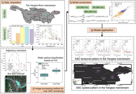
:Suspended sediment concentration (SSC) is an important indicator of water quality that affects the biological processes of river ecosystems and the evolution of floodplains and river channels. The in situ SSC measurements are costly, laborious and spatially discontinuous, while the spaceborne SSC overcome these drawbacks and becomes an effective supplement for in situ observation. However, the spaceborne SSC observations of rivers are more challenging than those of lakes and reservoirs due to their narrow widths and the broad range of SSCs, among other factors. We developed a novel SSC retrieval method that is suitable for the rivers. Water was classified as clear or turbid based on the Forel–Ule index, and optimal SSC models were constructed based on the spectral responses to SSCs in cases of different turbidity. The estimated SSC had a strong correspondence with in situ measurements, with a root mean squared error (RMSE) of 24.87 mg/L and a mean relative error (MRE) of 51.91%. Satellite-derived SSC showed good consistency with SSCs obtained from gauging stations (r2 > 0.79). We studied the spatiotemporal variation in SSC in the Yangtze main stream from 2017 to 2021. It increased considerably from May to October each year, with the peak generally occurring in July or August (ca. 200–300 mg/L in a normal year and 800–1000 mg/L in a flood year), while it remained stable and decreased to around 50 mg/L from November to April of the following year. It was high in the east and low in the west, with local maxima in Chongqing (ca. 80–150 mg/L) and in the lower Dongting Lake reaches (ca. 80–100 mg/L) and a local minima in the downstream of the Three Gorges Dam (ca. 1–20 mg/L). Case studies in the Yibin reach and Three Gorges Reservoir determined that local variation in SSCs is due to special hydrodynamic conditions and anthropogenic activities. The procedure applied to process Sentinel-2 imagery and the novel SSC retrieval method we developed supplement the deficiencies in river SSC retrieval.
1. Introduction
Suspended sediment (SS) in water bodies impacts biological processes in river ecosystems [1,2,3], the development of floodplains [4,5,6], and deposition in river channels [7,8,9], etc. Analyzing the distribution of the suspended sediment concentration (SSC) is critical for understanding the variation in deposition and erosion in aquatic ecosystems [10]. Regular SSC monitoring in rivers and lakes is implemented through the use of gauging stations, which manually collect water samples and then the mass of SS is measured in the laboratory [11,12]. Although this method is accurate and widely accepted by hydrologists, it is costly and time-consuming. In the main stream of the Yangtze River, only 17 gauging stations are capable of SSC measurement. The spatial discontinuity of observed SSC limits our understanding of river hydrodynamics and the interaction between SS and terrestrial ecosystems. Satellite remote sensing techniques have several advantages in SS mapping, including regular and low-cost coverage [13]. They provide effective supplementary observations for ground-based SSC monitoring techniques and can be combined with hydrodynamic models in studies of inland and coastal dynamics [14,15,16].
The strong backscattering feature of SS affects the absorption and scattering of light in the water column [17]; therefore, its concentration can be detected with remote sensing methods. Current satellite-based SSC retrieval methods roughly include empirical approaches [18,19,20], semi-analytical approaches [20,21,22,23], and semi-empirical approaches [24,25,26]. The empirical approaches directly establish the statistical relationships between the spectrum and the SSC, including band index regressions [27,28] and machine-learning methods [29,30,31]. These approaches only search for the expression with optimal correlation between spectra and in situ measurements, without considering the responses of the optical substances at the different wavelengths or the interactions among various bio-optical constituents. Semi-analytical approaches rely on the relationship between SSC and inherent optical properties (IOPs), including absorption and backscattering coefficients. These approaches use IOPs as a bridge to establish a link between a spectrum and SSC to emphasize the radiative transfer mechanism of optical components in a water body. Semi-analytical approaches have clear and interpretable physical mechanisms. However, they suffer from the uncertainty in the SSC–IOP relationship, which covaries with sediment size, shape, mineralogical composition, and other factors [32]. The semi-empirical method is an intermediate approach between the two methods described above. It considers the response characteristics of the spectrum to SSC in the band selection and the index construction, then uses a statistical method to establish the relationship between the spectral indices and the SSC. This method combines the physical and statistical properties of the spectrum without involving complicated radiation transfer mechanisms, eliminating the dependence on analytical hypothesis relationships.
Water optical classification is an effective approach to improving the model generalization and representativeness. Models constructed for SSC retrieval are limited by water constituents and are site-specific, which is related to the optical water type. To overcome these limitations, researchers have tended to conduct a water classification and then construct a retrieval model for each class for a region with complex optical properties. Previous studies have adopted the thresholds for optical classification, including single-band [25,33,34], band ratios [33], and a spectral index [13]. These approaches are fundamentally classified based on their spectral shape and magnitude, which is susceptible to atmospheric disturbance and observation conditions. The Forel–Ule index (FUI) is the quantitative representation of water color and is closely related to water turbidity [34,35]. It is resistant to aerosol disturbance and sensor observation geometry [36]. Therefore, it can provide a stable threshold for optical classification that is less disturbed by external conditions and will improve the consistency of SSC measurements among various sub-models.
Previous SSC studies have mostly focused on large or open waterbodies such as lakes [27,37], reservoirs [38,39], and estuaries [40,41], with only a few studies focusing on river systems. In the Yangtze River Basin, most previous studies have focused on Yangtze estuaries [10,42,43,44,45] and some large lakes (e.g., Dongting Lake, Poyang Lake, Taihu) [46,47,48], while few have considered the whole main stream of the Yangtze River. However, SSC retrieval in river systems is more challenging than in the lakes, reservoirs, and coastal waterbodies. First, there is limited availability of sensors for river SSC retrieval due to rivers’ narrow widths and sensor ground sampling distances (GSDs). Water color sensors such as the Geostationary Ocean Color Imager (GOCI) and the Ocean and Land Colour Imager (OLCI) have a GSD of hundreds of meters or even thousands of meters, which is a problem for river monitoring, particularly after excluding the land/water mixed pixels. Second, the adjacency effect (cross-radiation from surrounding areas that interfere with the optical signals of the water body received by the sensor [49]) would degrade the water spectrum. This effect impacts the inversion accuracy of SSC and even the accuracy of the water extraction. Third, rivers cover a broad range of SSCs and have more complex and changeable water optical types, leading to difficulties in high-precision SSC retrieval with sa ingle model. Finally, rivers span a wider geographical range and the corresponding aerosol types are changeable; therefore, more accurate atmospheric correction parameter settings are needed.
In this study, we developed a novel method of river SSC retrieval method using Sentinel-2 Multispectral Instrument (MSI) images and applied it to the main stream of the Yangtze River. The purpose of this study was to (1) establish a remote sensing inversion model to estimate the SSC along the Yangtze River and to (2) analyze the spatiotemporal distribution of SSC for the whole streams and some case study reaches of the Yangtze River from 2017 to 2021.
2. Materials and Methods
2.1. Study Area
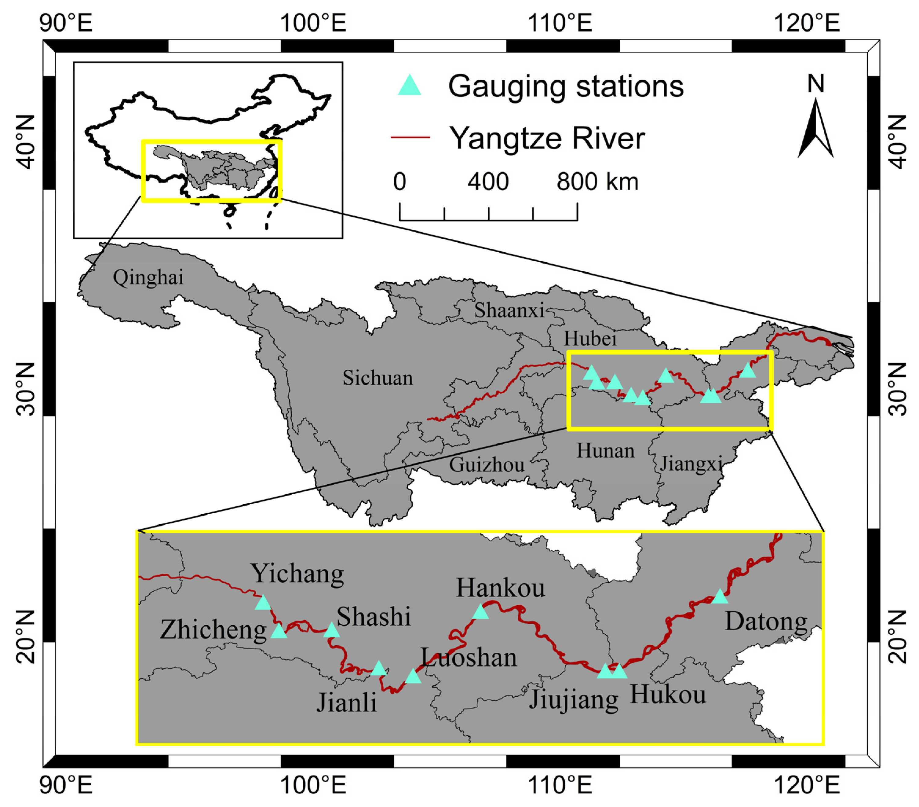
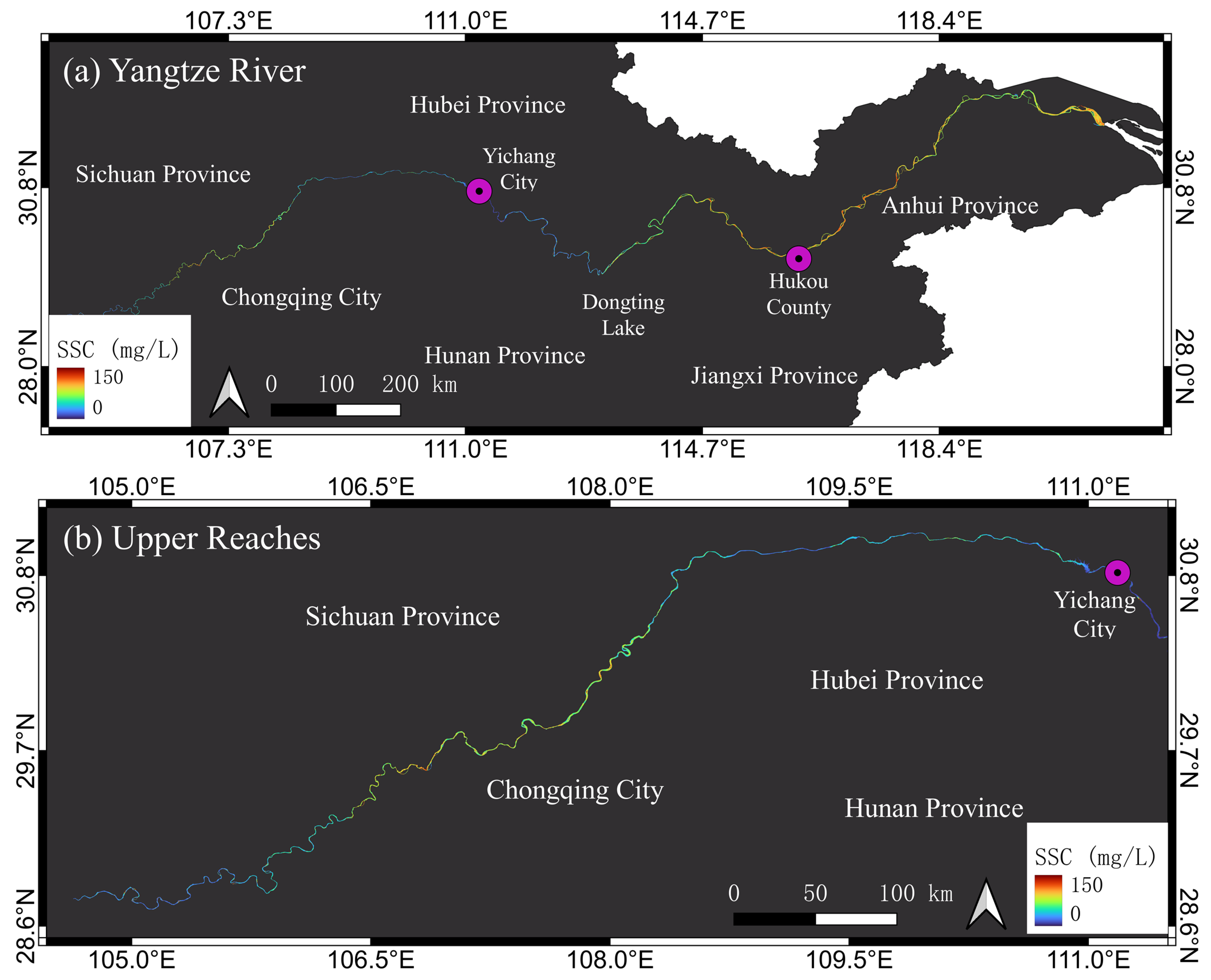
The Yangtze River is the longest river in China, at nearly 6300 km (Figure 1). The huge Yangtze drainage basin, covering a catchment area of 1.94 × 10⁶ km2, can be divided into three sections: the upper, middle, and lower reaches [50]. The river between the Yangtze source and Yichang City, Hubei Province, is the upper reach, with a length of 4504 km, width between 0.5–1.5 km, and depth of between 5–20 m. The middle reaches cover the area from Yichang City to Hukou County of Jiujiang city, Jiangxi Province, with a length of 955 km, width of 1–2 km, and depth of 6–15 m. Hukou County to the estuary represents the lower reaches, with a length of 938 km, width of 2–4 km, and depth of 10–20 m. Above Yibin City, Sichuan Province, is the Jinsha River, whose average width is 200 m. The narrow river width, the mountain shadow, and the complex hydrodynamic conditions make it difficult to detect using the MSI sensor. Due to these limitations, our research only focused on the main stream from Yibin to the estuary (Figure 1).
2.2. Gauging Stations Data
The SSCs from nine gauging stations from 2015 to 2020 were used for model calibration and validation. These data were provided by the Changjiang Water Resources Commission (CWRC), and the locations of the gauging stations are shown in the Figure 1. The gauging station data included the daily water discharge and SSC values from nine sites. The water samples were obtained manually and taken to the laboratory for SSC measurement. Each water sample was weighed and then dried in an oven for 2 h at 100–110 °C. The mass of the residue was determined and divided by the mass of the water sample to acquire the SSC. In all, 19,362 gauging station measurements were obtained. When the sampling point was contaminated by cloud/cirrus, shadows, sun glint, or boats/ships, the matching spatial window was expanded to 3 pixels to increase the number of satellite–ground data pairs. A total of 488 concurrent data pairs were ultimately obtained, with an SSC range from 2 to 850 mg/L (Table 1).
2.3. Sentinel-2 Image Processing
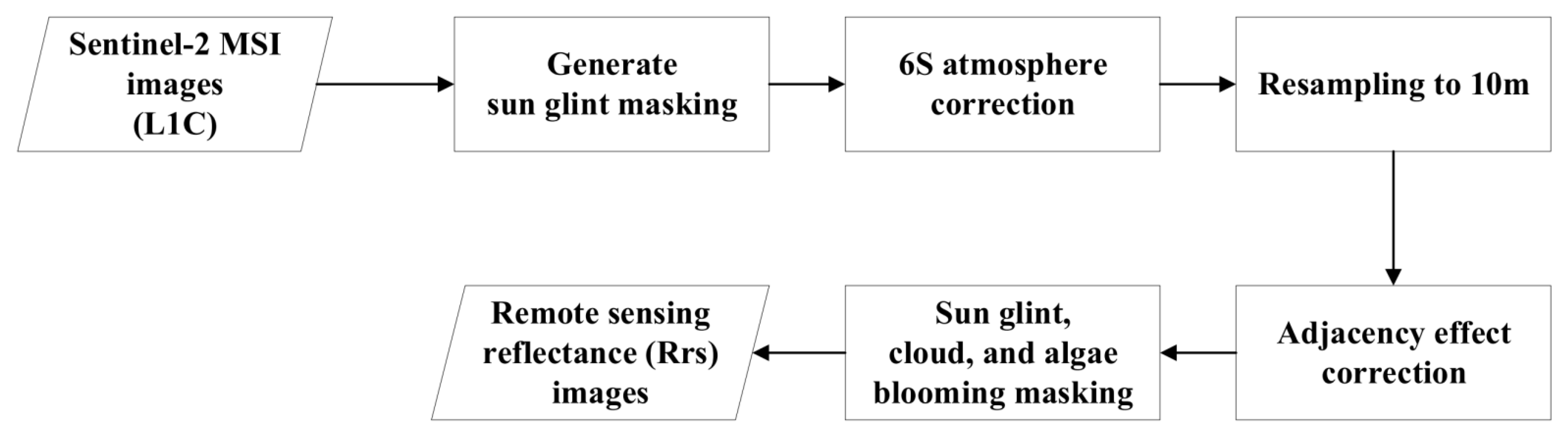
Sentinel-2 Level-1C (L1C) top-of-atmosphere (TOA) images of the Yangtze River from 2016 to 2021 with a cloud cover of less than 40% were obtained from the Google Earth Engine (GEE). We used all available MSI L1C images over the study area and resampled them to 10 m. In all, 488 images were used in this study. The graphic processing step refers to Figure 2.
The second simulation of satellite signal in the solar spectrum (6S) [51] model was used for the atmospheric correction. Continental, biomass burning, or urban aerosol was chosen as the aerosol profile type. Sensor observation angle, solar observation angle, scene date, and solar irradiance in each band were obtained from the image metadata. The daily aerosol optical depth (AOT) at 550 nm was acquired from the MODIS MCD19A2 product [52], and monthly AOT at 550 nm was acquired from the MODIS MOD08 product [53]. The total column atmospheric water vapor was obtained from National Centers for Environmental Prediction–National Center for Atmospheric Research (NCEP–NCAR) global reanalysis data [54]. Daily total column ozone data were acquired from the NASA Goddard Earth Sciences Data and Information Services Center. Altitude was obtained from the Shuttle Radar Topography Mission (SRTM) digital elevation dataset. Then, the remote sensing reflectance () above the surface water was calculated using Equations (1)–(3):
where L is the TOA radiance from Sentinel-2 L1C images; xa, xb, and xc are atmospheric correction coefficients obtained from the 6S process; ρ is the surface reflectance; Edir is the irradiance produced by solar radiation from the direction of the sun; Edif represents the irradiance in other directions due to aerosol and molecular scattering. The spectral reflectance of skylight at the air–water interface, rsky, was set to 0.0245 in this study, which typically ranges from 0.022 in calm weather to 0.025, with wind speeds of up to 5 ms−1 [39].
The adjacency effect depends on the aerosol height distribution and can influence the accuracy of image spectra after atmospheric correction [55]. The cross–radiation from bright river banks, particularly from the urban areas, alters the optical signal received by the sensor [56]. We therefore minimized the adjacency effect by reducing the pixel-to-background contrast within the kernel window [57]. This method consists of two steps: the calculation of the average remote sensing reflectance () within the kernel window of each pixel, with a window radius of 1 km (Equation (4), and then the correction of the adjacency influence using Equations (5) and (6):
where N corresponds to the number of pixels in the selected range; Rrs_ac is the Rrs after adjacency correction; q is the ratio of the diffuse (τdif) to direct (τdir) ground-to-sensor transmittance obtained from the 6S process.
Sun glint, also known as a transient anomaly, happens when sunlight reflects directly from the surface water to the sensor [58]. Other features, including whitecaps, ships, and cirrus, can influence the accuracy of the inversion models and water-quality observations. Pure water has a large absorption in the near-infrared and short-wave infrared spectra. The TOA radiance at Band 12 (centered at 2200 nm) above the water surface does not include any water-leaving radiance. It can be considered the summation of atmospheric path radiance and sky radiance reflected by the water surface, while the latter includes the sun glint. We proposed a sun glint index (SGI) based on the spectral features at Band 3 and Band 12 and then determined the threshold via repetitive trial-and-error tests. We found that pixels with SGI smaller than −0.5 were free of sun glint contamination. The index was defined as:
where B12 and B3 represent the TOA radiances in the twelfth and third bands, respectively. Pixels with an SGI smaller than −0.5 were considered free of sun glint contamination.
To analyze the accuracy of satellite-derived Rrs, we used the L2A products captured at the same time to evaluate the consistency of Rrs between our method and L2A standard products [59].
2.4. Water Optical Classification
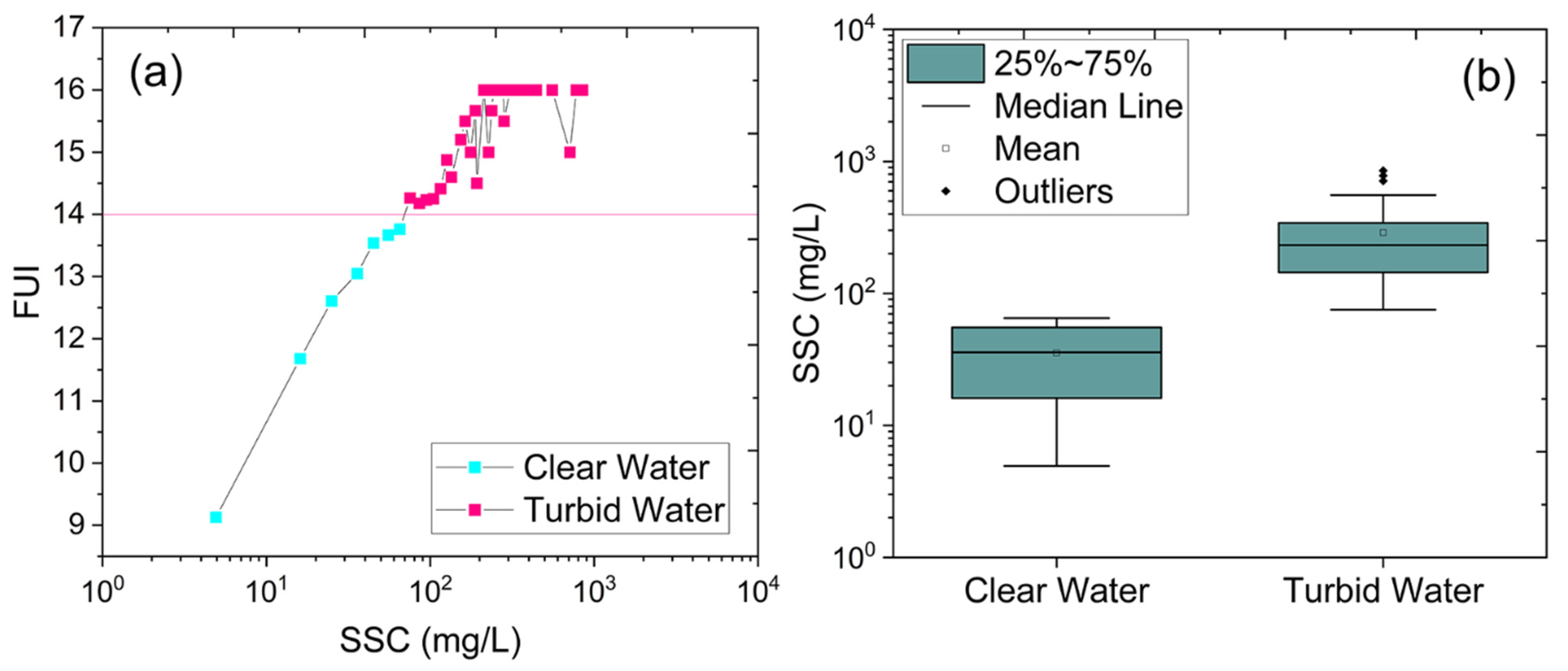
Water optical classification improves the model SSC representation, particularly with regard to the broad range of SSCs. The visible spectrum is sensitive to low and medium SSC (ca. <50 mg/L), but it becomes saturated in high-turbid waters (ca. >50 mg/L) [60]. The SSC in the Yangtze has a wide range from 20 to 2500 mg/L [43]. Thus, we classified waterbodies into two types (clear water and turbid water) using the FUI and then constructed a retrieval model for each type. Five Sentinel-2 bands (with central wavelengths at 443, 490, 560, 665, and 705 nm) were used to calculate the hue angle (α) in color space. Then, the FUI was obtained according to the 21-class FUI look-up table. The calculation method is detailed in a previous study [61].
We determined the classification threshold based on the relationship between the FUI and the measured SSC. The FUI was calculated based on the Sentinel-2 spectrum in the satellite/ground data pairs. The data pairs were reordered from small to large according to the SSC. We grouped data pairs at intervals of 10 mg/L and calculated the average SSC and corresponding average FUI for each group, from which we drew a line chart (Figure 3a). When the SSC was low, the FUI increased with increasing SSC. When the FUI value exceeded 14, the index no longer increased monotonically with increasing SSC but rather fluctuated in the range of 15–17. Thus, an FUI = 14 could be used used as a classification threshold to divide natural water into two types, clear and turbid water. The average SSC differed between the two types of water, being 35.34 ± 21.55 mg/L for clear water bodies and 288.97 ± 208.21 mg/L for turbid waters (Figure 3b).
2.5. Model Construction
To establish the SSC retrieval model, the in situ SSC measurements were processed to be temporally collocated within 12 h of the associated Sentinel-2 derived Rrs. The Rrs spectra whose values in the near-infrared (VIS-NIR: B1-B8A) bands were smaller than zero were considered outliers and were removed.
We adopted a semi-empirical method to construct the SSC inversion model. We examined the spectral responses to SSC and discovered that, when the SSC was low (SSC < 50 mg/L), the red and green bands showed the most sensitive response. The spectral signal in the VIS band became saturated as the SSC increased, and the sensitive band switched to the NIR spectral region. Previous studies have shown that the band-switch method with the VIS–NIR band for SSC inversion can achieve excellent results [24]. Hence, we divided data into two water types using the FUI and selected the optimal performance by trial-and-error for each class: B4 (665 nm)/B3 (560 nm) for clear water (r2 = 0.54) and B8A (865 nm)/B4 (665 nm) for turbid water (r2 = 0.57). We built various algorithms using linear, exponential, logarithmic, and other formulae using the chosen indices, then selected the model with the best fitness as the final model for each type of water body.
2.6. Accuracy Metrics
The average relative error (MRE) and root mean square error (RMSE) for the modeled values and in situ measurements were used as accuracy evaluation indices:
where Y and Y′ are in situ measurements from gauging stations and modeled data respectively, and n is the total number of sampling points.
3. Results
3.1. Validation of Sentinel-2 MSI Rrs
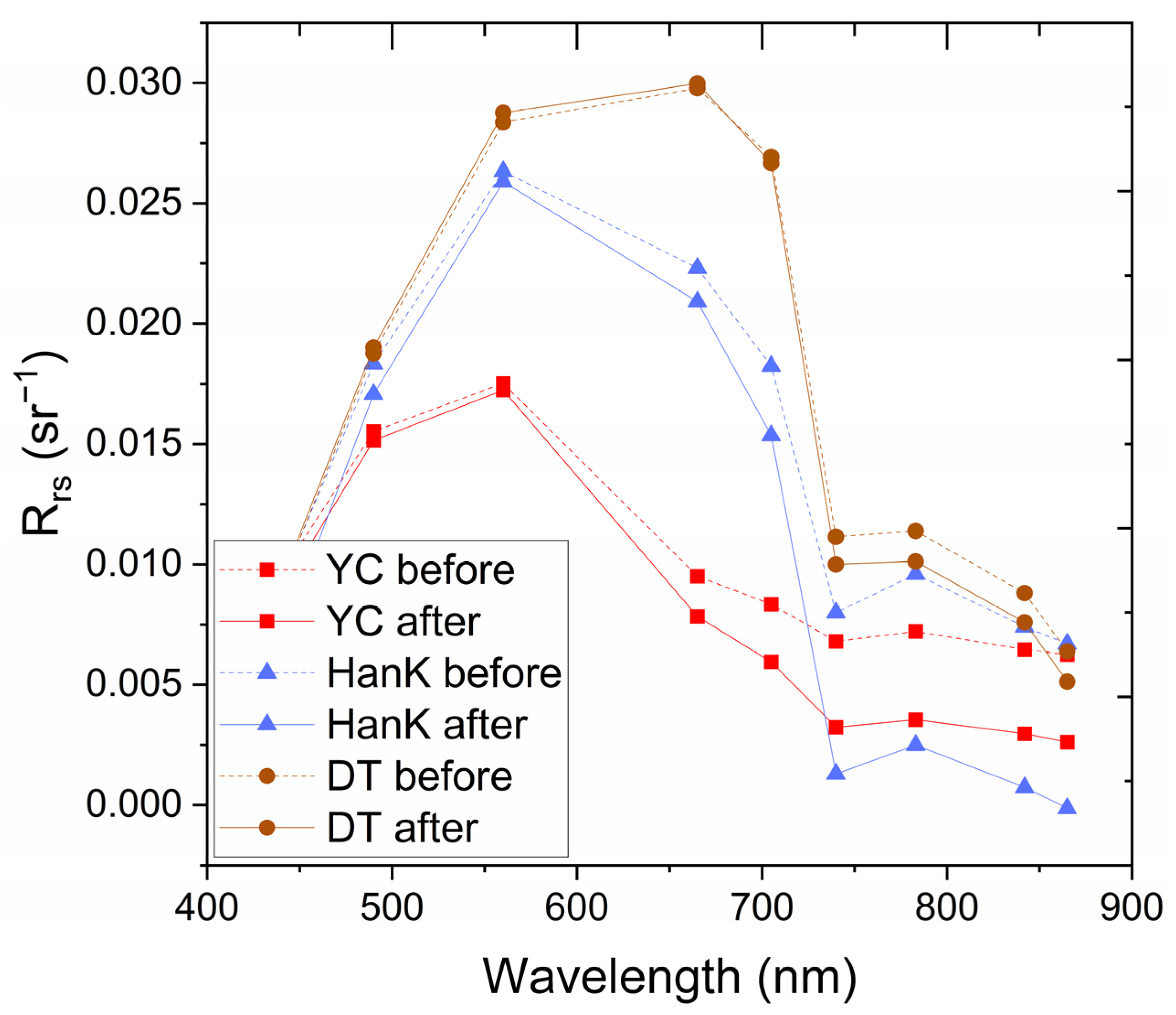
We compared the Rrs before and after adjacency correction to illustrate its necessity and the effectiveness of the correction. We selected the water spectrum at the center of the river at the gauging stations in Yichang, Hankou, and Datong for comparison (Figure 4). The results implied that the spectrum with the adjacency correction was slightly lower than before the correction. We calculated the mean relative difference (MRD) of the corrected and original spectrum to evaluate the performance of the adjacency correction. In the blue and green bands (the center of wavelength smaller than 600 nm), the adjacency effect had a weak impact on the spectrum with MRD of 3.86%, 10.78%, and 1.48% at Yichang, Hankou, and Datong, respectively. However, the adjacency effect had a more significant impact on the spectrum in the red and NIR bands (the central of wavelength larger than 600 nm), with MRD of 43.63%, 61.95%, and 9.43%, respectively. In addition, the water spectrum at Hankou (MRD = 44.89%) and Yichang (MRD = 30.37%) displayed larger differences after adjacency correction than Datong (MRD = 6.78%). There were large urban areas near Yichang and Hankou Stations, while Datong Station was surrounded by vegetation and a small area of rural housing. In addition, the river was wider in the Datong reach (1800 m) than in the Yichang (400 m) and Hankou (1100 m) reaches. Thus, the adjacent bright albedo in the Yichang and Hankou reaches was responsible for more severe interference in the Rrs. For SSC retrieval in the river, if the adjacency effect was ignored, the Rrs in the red and NIR bands will be higher than the actual value, resulting in an overestimated SSC.
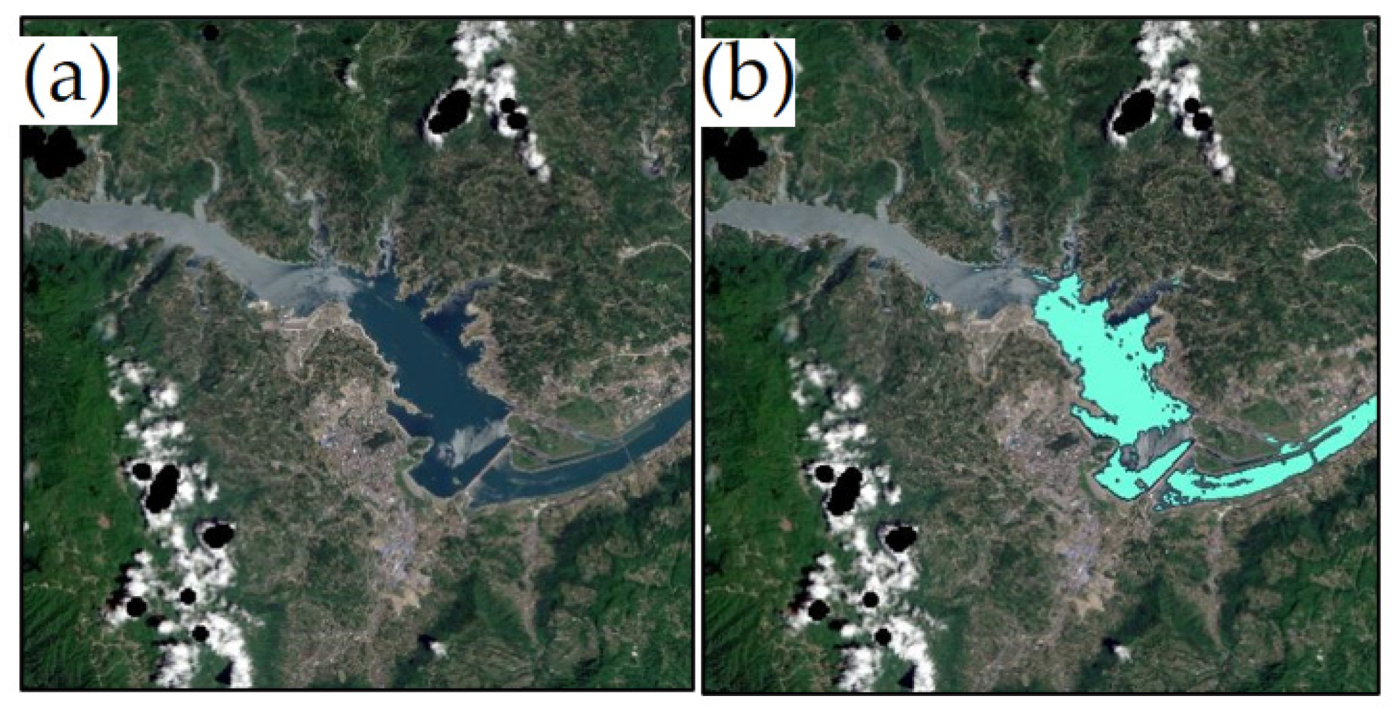
We selected an image at the Three Gorges Dam (captured on 10 May 2020) to examine the effect of sun glint removal. We calculated the SGI from the TOA image, set the threshold at −0.5 to generate a mask, and then conducted sun glint removal on the Rrs image. Figure 5 shows the images before and after sun glint removal, respectively. The region covering the white or gray colors is severely contaminated by sun glint, while the pure water region displays relatively low reflectance (Figure 5a). The SGI therefore effectively separated the contaminated and pure water regions in terms of sun glint removal (Figure 5b).
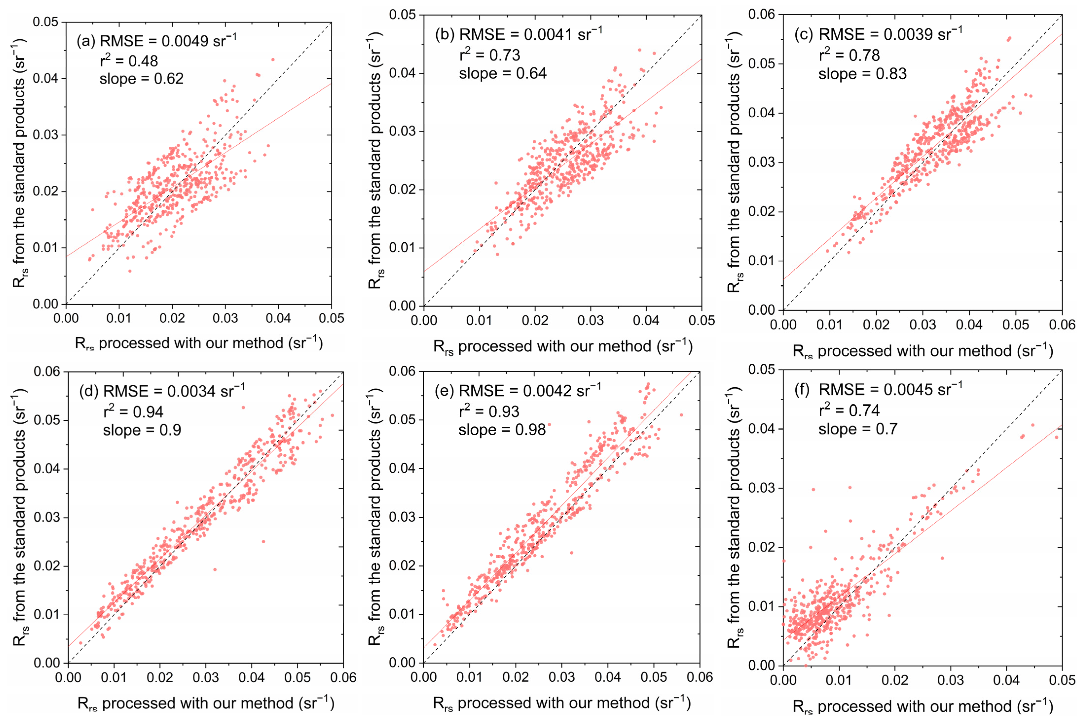
Due to the lack of a quasi-concurrent field spectrum, Rrs was validated using Sentinel-2 Level-2A (L2A) surface reflectance products. A total of 94 images were used, with 500 sampling points extracted. We compared the Rrs processed with our method to that from the standard products in the B1–B5 and B8A bands. Their consistency was quantitatively evaluated according to the coefficient of determination (r2) slope of the optimal fit line between Rrs processed with our method and that from a standard product, and the RMSE. Figure 6 depicts the accuracy of Rrs in the six bands referred to above. The points in the figure are distributed along the 1:1 line, indicating that the preprocessing method used in this study was satisfactory. The Rrs in the B3 (560 nm), B4 (665 nm), and B5 (704 nm) bands had the highest consistency between the two datasets (r2 > 0.78, 0.8 < slope < 1, RMSE < 0.0042 mg/L), followed by the B1 (443 nm), B2 (492 nm), and B8A (865 nm) bands.
3.2. Validation of the SSC Retrieval Model
Among the 488 data pairs, 390 (80%) were used for model training and 98 (20%) were used for an independent evaluation of model accuracy. For an FUI ≤ 14, the two spectral indices (B4 (665 nm) and B4/B3 (665/560 nm)) and the FUI values were used as model parameters. For an FUI > 14, the two spectral indices (B8A (865 nm) and B8A/B4 (865/665 nm)) and the FUI were used as model parameters. The SSC evaluation model was expressed as:
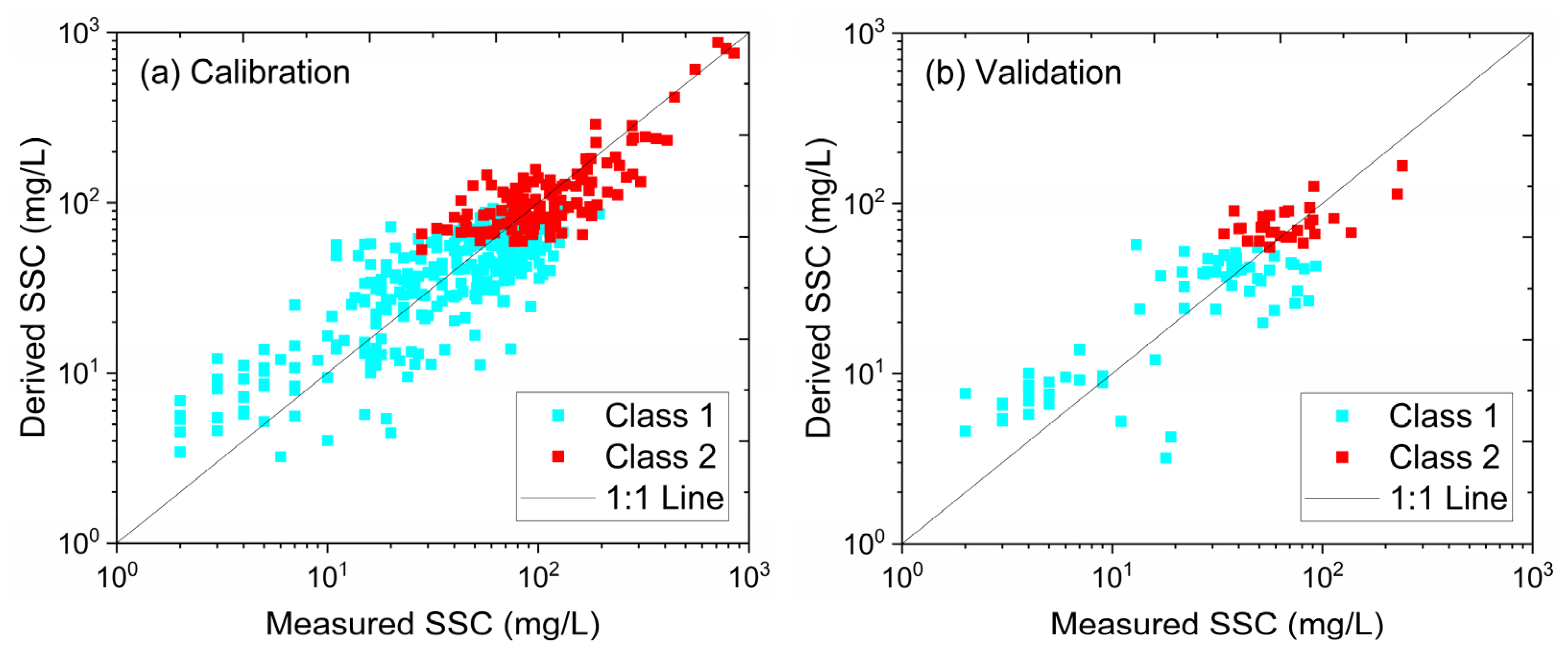
We analyzed the agreement between the modeled SSC and measured SSC. The r2 value was 0.85 (p < 0.001) for the calibration data and 0.61 (p < 0.001) for the validation data (Figure 7). Most modeled and measured SSC points were distributed along the 1:1 line, indicating satisfactory model performance. The RMSE and MRE of our model were 35.62 mg/L and 47.35%, respectively, for the calibration data, while the corresponding values were 24.87 mg/L and 51.91% for the validation data. In clear water, the scatter points were relatively dispersed. The RMSE and MRE for the calibration and validation datasets were 24.12 mg/L and 53.55%, and 20.76 mg/L and 54.04%, separately. The detailed statistical attributes and model performance were listed in Table 2. Our model performed better for turbid water than for clear water. This is attributed to the low SSC in the water body, resulting in the water body being dominated by other optically active substances, e.g., chlorophyll and chromophoric dissolved organic matter (CDOM), which made it difficult to discriminate the optical signal of SS [62].
3.3. Temporal Characteristics of SSC
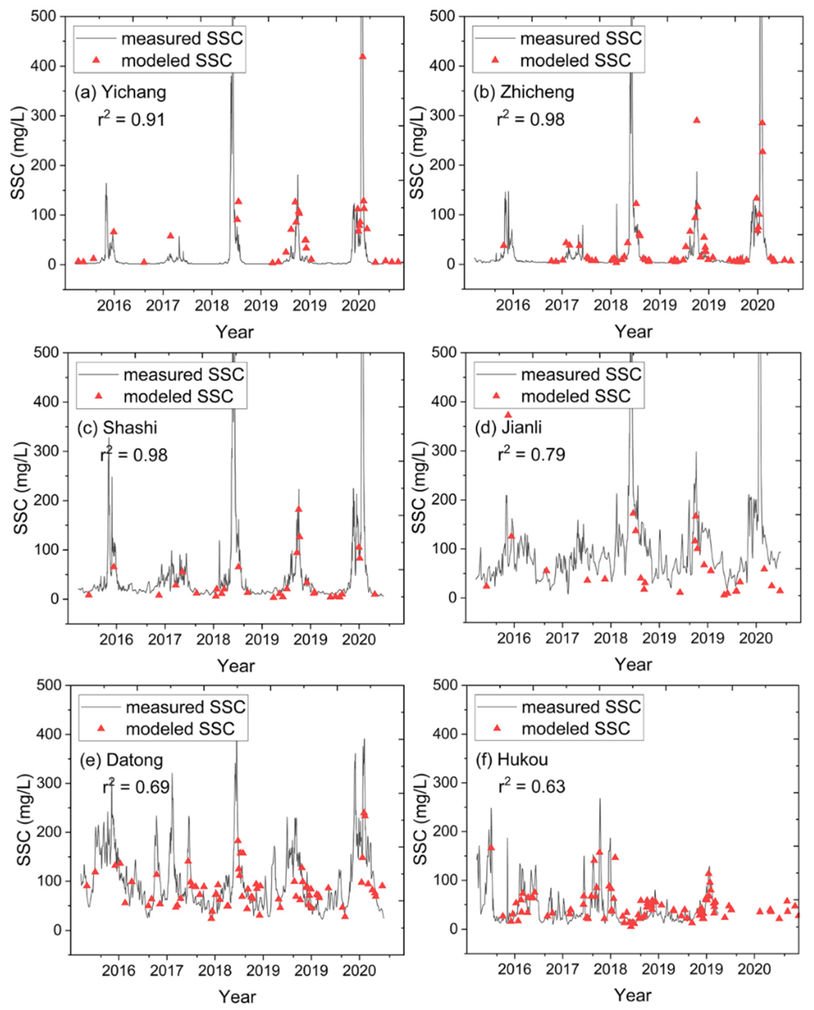
We implemented the proposed model at six gauging stations (Yichang, Zhicheng, Shashi, Jianli, Datong, and Hukou) and analyzed the consistency in SSC between modeled and in situ data. The modeled SSC showed good consistency with the SSC obtained from the gauging stations, and the r2 values of 0.91, 0.98, 0.98, 0.79, 0.69, and 0.63 for Yichang, Zhicheng, Shashi, Jianli, Datong, and Hukou, respectively, and the two datasets showed a significant difference at each station (p < 0.001). The SSC retrieved from our method was generally compatible with the observations from gauging stations. Our method accurately depicted the trend in SSC variation and captured the peaks and troughs of SSC variation (Figure 8). However, due to the revisit period and cloud masking, the availability of Sentinel-2 observations strongly restrained the ability to monitor SSCs’ monthly characteristic and extreme hydrological events.
We further studied the temporal characteristics of SSC as revealed by satellite-based data from 2016 to 2020. The modeled SSC increased to a high level and peaked in the wet season, while it fell to a minimum in the dry season (Figure 8). The SSC increased from May to October each year, with the peak generally occurring in July or August (ca. 200–300 mg/L in a normal year and 800–1000 mg/L in a flood year). It did not change significantly from November to April of the following year, remaining at low levels (ca. <50 mg/L). This pattern was strongly synchronized with the hydrological circulation.
3.4. Spatial Distribution of SSC
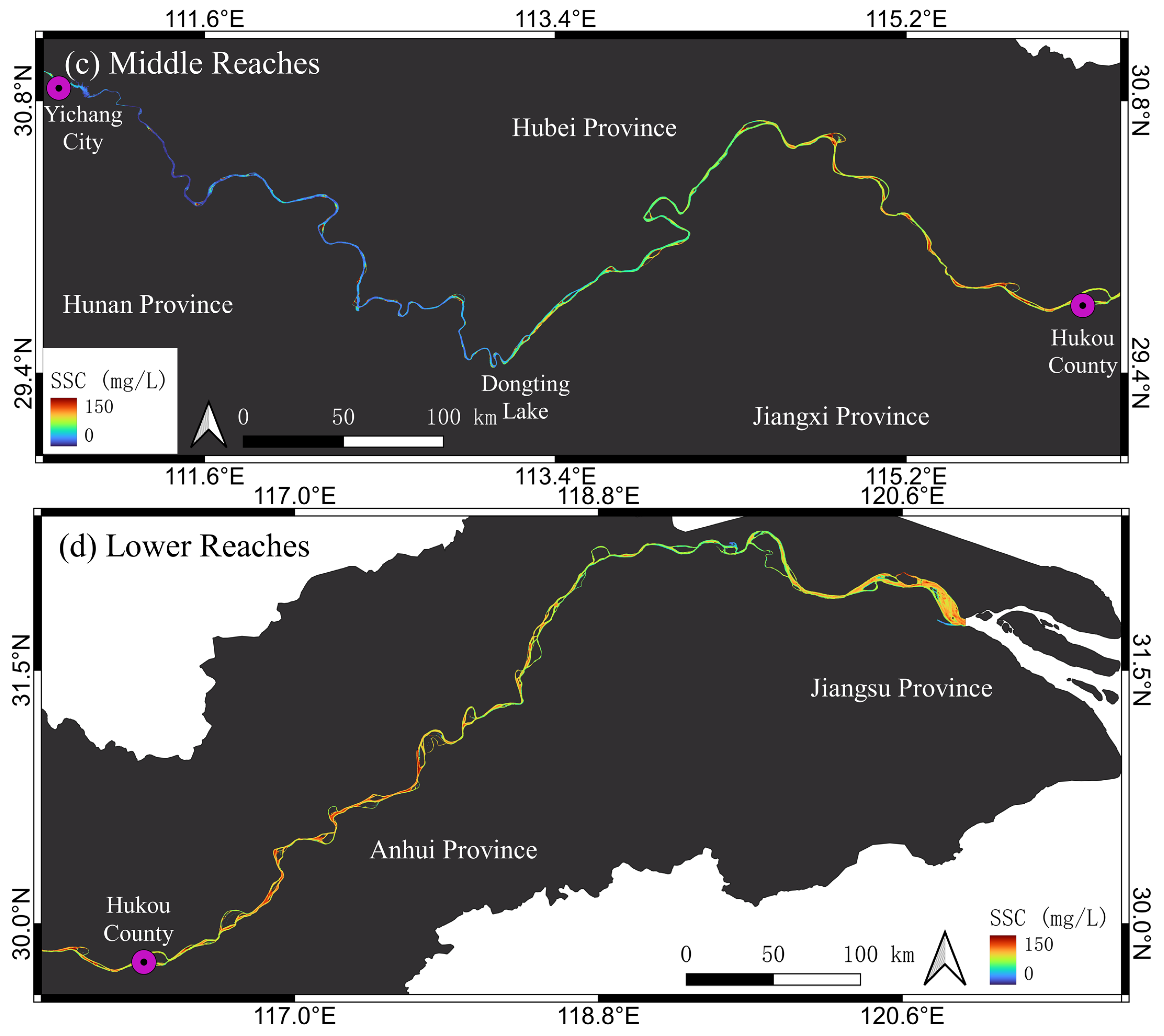
To study the spatial pattern of SSC, we aggregated the Rrs from 2017 to 2021 and retrieved the median SSC of the main stream of the Yangtze. It showed a spatial distribution pattern of being low in the west and high in the east (Figure 9). The median SSC ranged from 5.98 to 175.36 mg/L over the study period, with a median of 59.06 mg/L. The median SSCs in the upstream, midstream, and downstream regions were 51.32, 58.80, and 98.21 mg/L, respectively.
In the upper reaches of the river, the SSC ranged from 18.63 to 175.36 mg/L, generally remaining at a low level. There was a local increase in the central region of Chongqing. We speculate that this was due to the extreme weather during the study period. In addition, in the 2020 flood season, catastrophic rainstorms occurred in Sichuan Province and Chongqing City, resulting in a large amount of sediment entering the Yangtze River channel [63]. The increase in local SSC therefore affected the 5-year average value. In the middle reaches, the SSC was between 5.98 and 124.20 mg/L, with a standard deviation of 56.79 mg/L, indicating significant regional variation. Taking Dongting Lake as the dividing point, the SSC levels on each side were noticeably different. This can be ascribed to the impoundment of the Three Gorges Reservoir and the sediment retention by the dam, which caused the water in the downstream reaches to be extremely clear. However, Dongting Lake conveyed a huge amount of SS to the river through its mouth in the northeast corner, resulting in a significant increase in SSC. In the lower reaches, the SSC ranged from 62.03 to 132.89 mg/L, always remaining at a high level. It was relatively homogeneous compared to the upper and middle reaches. Zhao et al. [64] examined the spatial distribution of water clarity (Secchi depth, SD) in the Yangtze River’s main stream from 2017 to 2020, and discovered that there was a local turbidity in Chongqing and relatively clear downstream water in the Three Gorges Dam, which was consistent with the SSC spatial pattern discovered in this study.
3.5. Case Study
SSC is closely related to local hydrodynamic conditions and flood events. We attempted to briefly construct the association between satellite-derived SSC and local hydrodynamic conditions to examine the SSC model’s ability to reflect local SSC characteristics. We selected the Yibin reach and the Three Gorges Reservoir as a case study.
3.5.1. Yibin Reach
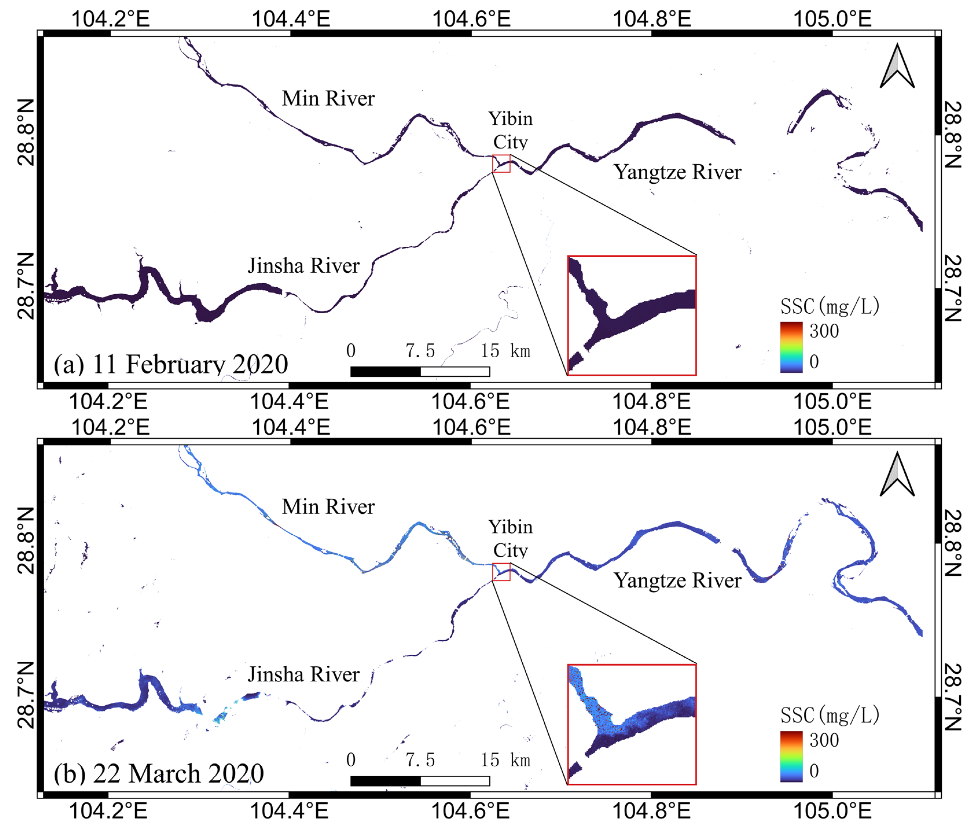
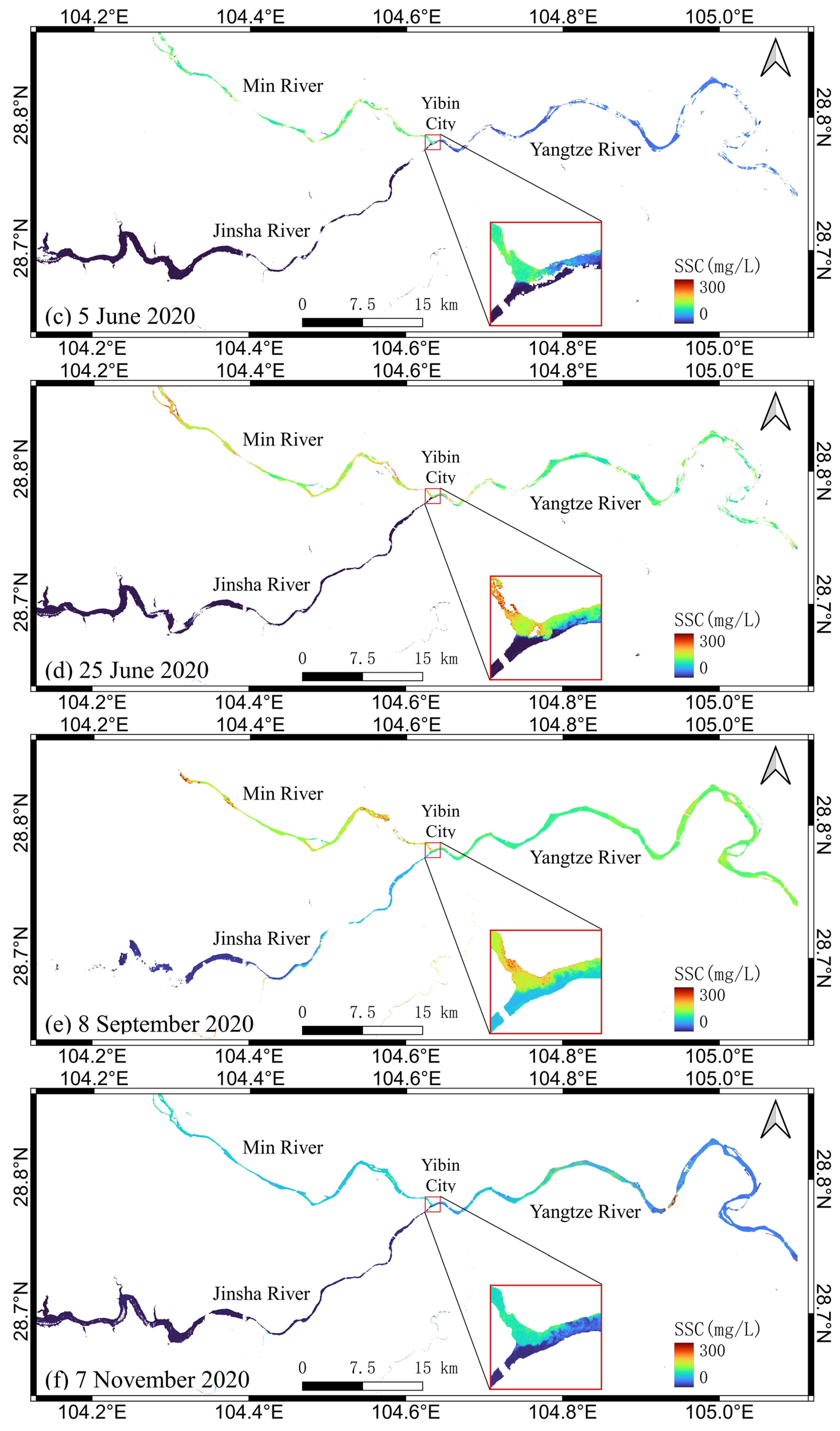
We applied the SSC retrieval method to three Sentinel-2 MSI images (11 February 2020, 22 March 2020, 5 June 2020, 25 June 2020, 8 September 2020, and 7 November 2020) to study the spatiotemporal distribution of SSC at the Yibin Reach (Figure 10). The Yibin Reach in Sichuan Province is part of the Yangtze River’s upper reaches. It is located at the confluence of the Jinsha and Min rivers, and the different sediment loads from the two rivers result in it representing a clear dividing line. In February, the SSC was spatially homogeneous, with a constantly low concentration (Figure 10a). SSCs in the Min River, Jinsha River, and Yangtze main stream were 4.26, 1.84, and 3.21 mg/L in February, respectively. From March to June, the SSC gradually revealed obvious spatial variations with a clear dividing line at the confluence of the Min River and the Jinsha River (Figure 10b–d). The average SSC in the Min River increased dramatically, from 43.56 mg/L to 133.2 mg/L, while the average SSC in the Jinsha River remained low (about 5 mg/L). In September, the SSC in the Min River slightly changed compared to previous months, but the mean September SSCs of the Min River, the Jinsha River, and the Yangtze main stream were 173.94, 82.76, and 132.31 mg/L, respectively (Figure 10e). In November, the SSC began to drop in the entire area as the dry season arrived, and the mean SSCs of the Min River, the Jinsha River, and the Yangtze main stream were 72.39, 12.7, and 66.56 mg/L, respectively (Figure 10f). In order to alleviate serious soil erosion in the Jinsha River watershed, Xiangjiaba hydropower stations were built in the lower reaches of the Jinsha River to regulate the discharge and sediment loads from the upstream [65,66]. Since the Xiangjiaba station started operating in 2013, the sediment load from the Jinsha River to the Yibin reach has been significantly reduced. According to the Yangtze River Sediment Bulletin, the average SSC at the Jinsha River outlet was 1660 mg/L from 1956 to 2010, but it decreased to 1010 mg/L and 18 mg/L in 2012 and 2013, respectively, while the average SSCs at the Min River outlet were 535, 240, and 270 mg/L, remaining relatively stable [67,68]. The hydropower station has effectively intercepted sediment loads and reduced the SSC in the lower Jinsha River. Thus, the different sediment loads of the Min River and Jinsha Rivers led to the obvious spatial heterogeneity of SSC at the confluence of the two rivers (Yibin Reach), and the SSC was high in the north and low in the south, with a clear dividing line.
3.5.2. Three Gorges Reservoir
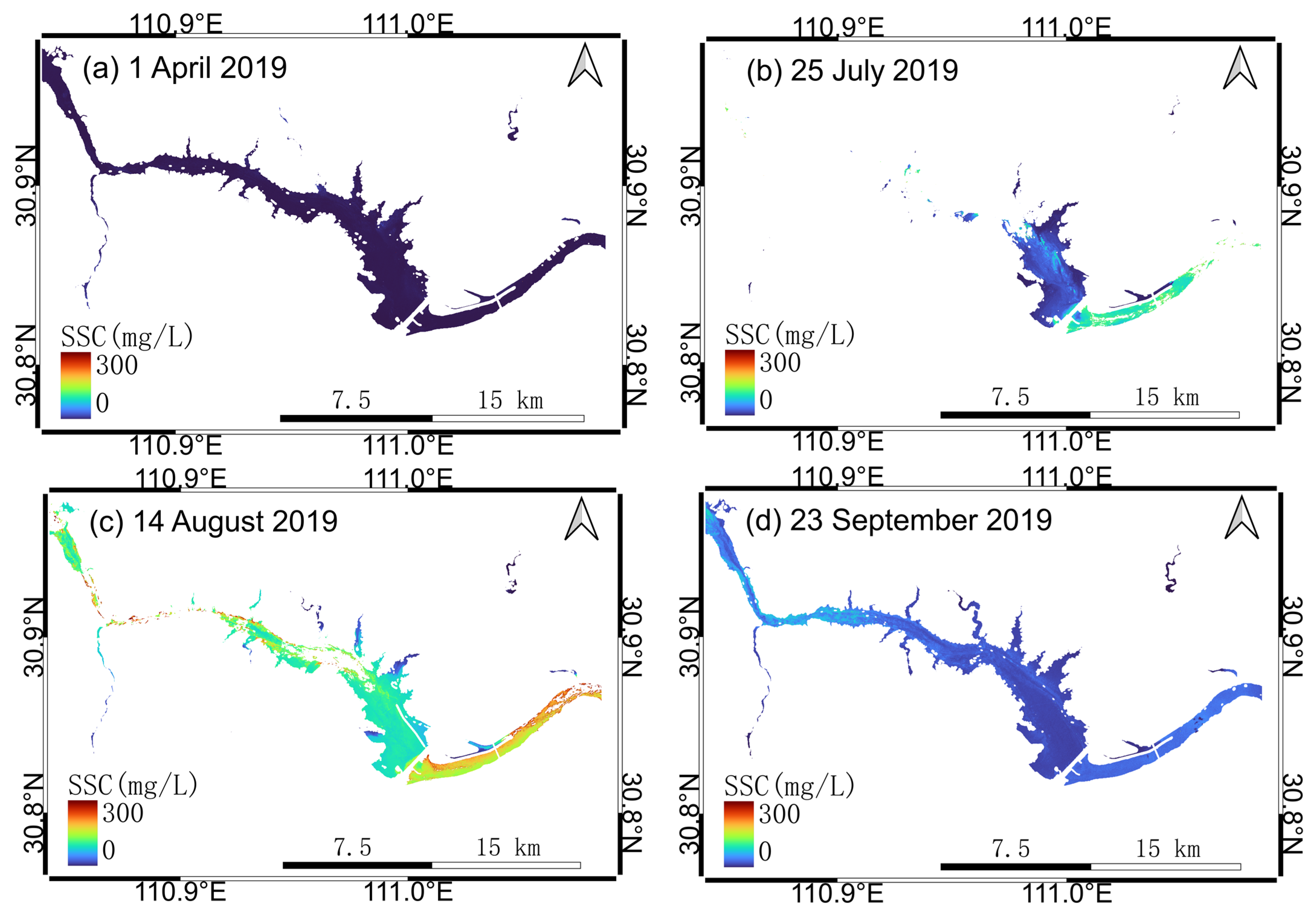
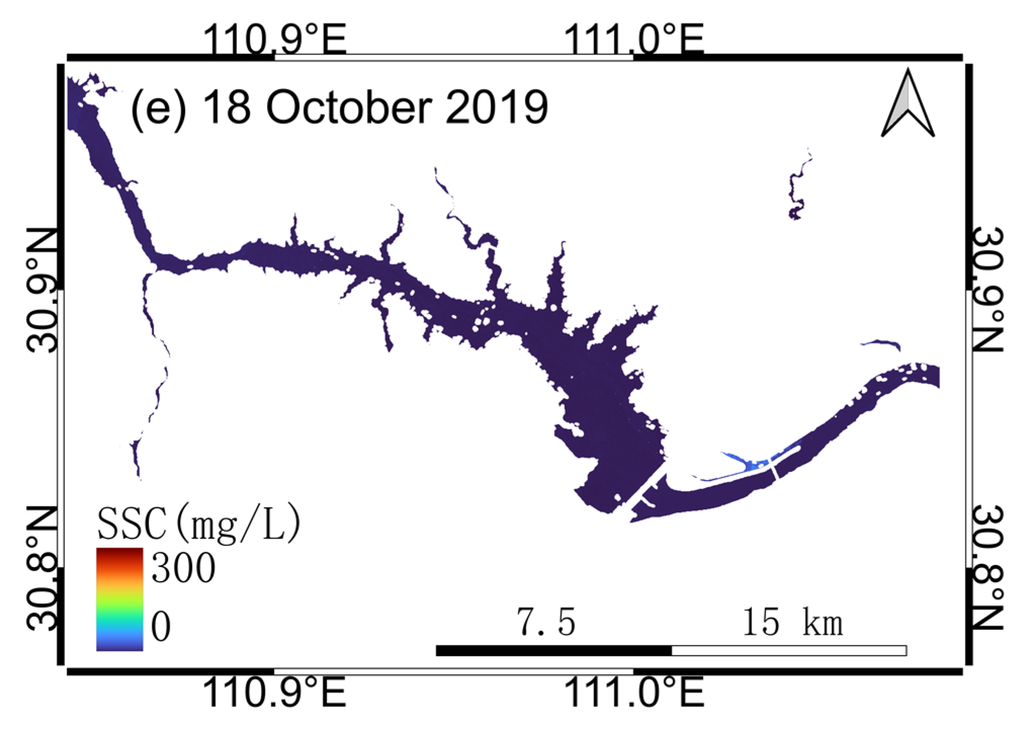
We applied the proposed method in the Three Gorges Reservoir and studied the spatiotemporal distribution in SSC. Figure 11 shows the SSC variation in SSC during the year. In April, it remained at a low level and there was no obvious spatial variability, with an averaged SSC of 3.84 mg/L. From July to August, the mean SSC increased from 77.41 to 183.48 mg/L and displayed an increasingly heterogeneous pattern. Taking the dam as a dividing line, the SSC on the west side of the dam was low, but it increased rapidly on the east side. As sediment was discharged into the reservoir during the flood season, the Three Gorges Dam discharged muddy water via the sand discharge holes at the bottom of the dam [69,70]. Due to interception by the dam, the SS in the area upstream of the dam was deposited on the bottom of the channel resulting in a reduction in the surface water [71]. As a result, remote sensing imagery revealed relatively clear water to the west of the dam and relatively turbid water to the east. In autumn, the mean SSC decreased to 31.59 mg/L on September 23 and 4.49 mg/L on October 18 (Figure 11), returning to the levels observed in spring. The spatial pattern became homogeneous. During this period, the amount of sediment from the upstream decreased, and the Three Gorges Reservoir began to accumulate clean water, allowing the benefits of transportation and power generation to be fully realized [72].
4. Discussion
4.1. Comparisons of Various SSC Retrieved Models
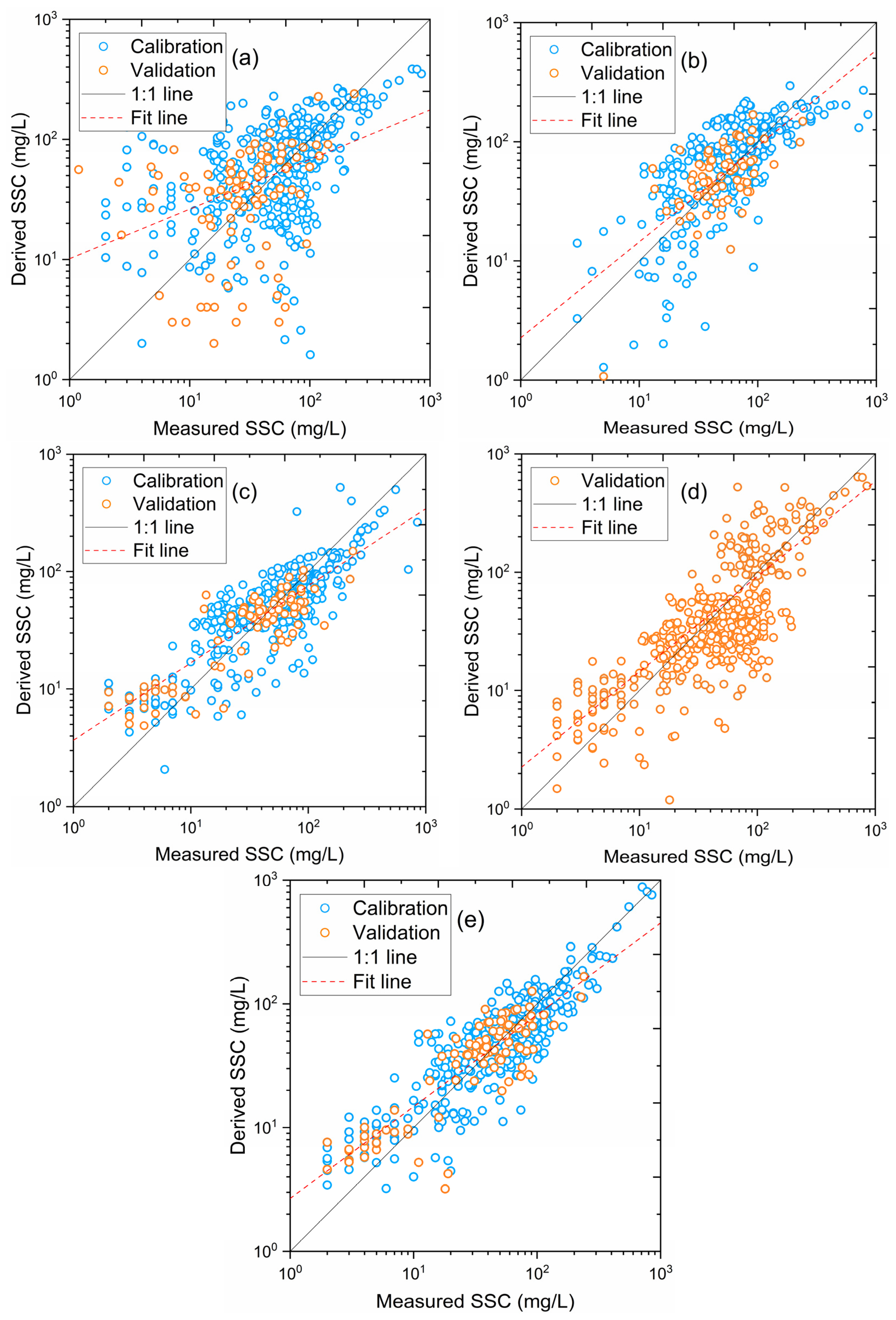
We subsequently compared our model to four state-of-the-art models [33] (Table 3) and analyzed their differences. Then we considered the options for SSC retrieval for rivers. We recalibrated the parameters of the other selected methods with the SSC obtained from gauging stations, with the exception of the SOLID model [33]. SOLID was trained with a machine-learning approach (mixture density network) with the associated parameters encapsulated. Figure 12 shows the performances of these models using the in situ dataset (n = 484).
Our model had the best SSC retrieval accuracy (RMSE = 24.87 mg/L, MRE = 51.91%), followed by SOLID and the model proposed by Yue et al. [13] (hereinafter, the Yue model). The model described in Cai et al. [73] (hereinafter, the Cai model) uses both red (665 nm) and NIR (865 nm) bands for SSC retrieval without water classification. The Cai model performed poorly for clear water (SSC < 500 mg/L), with a slight underestimation for turbid water (SSC > 500 mg/L). The model described in Hou et al. [74] (hereinafter, the Hou model) only uses visible bands (560 and 665 nm) for SSC retrieval, which resulted in a weakness for high-turbid water observations. The Hou model produced a negative SSC for extremely clear water (SSC < 50 mg/L) and severe underestimations for turbid water, particularly for SSCs > 200 mg/L. In summary, the Cai model and Hou models performed poorly, with an MRE > 100% and RMSE > 30 mg/L, while SOLID, the Yue model, and our model significantly outperformed those, with an MRE < 60% and RMSE < 30 mg/L. Hence, in the case of the Yangtze River, our model has the potential to generate reasonably accurate SSC products.
We identified several critical issues affecting SSC retrieval for rivers. First, compared to small and medium lakes and reservoirs, a broad range of SSCs must be considered in model development. Water optical classification is a recommended approach to improve model generalization. Second, due to the vibrant hydrodynamic conditions, water optical properties might have significant variation in the dry and wet seasons. Thus, the selected calibration and validation data should be sufficient and cover as many different seasons as possible. Third, the optical classification method should consider the dominant optical active constituents. For example, some researchers have used the MCI as a classification index for waters abundant with floating algae. The FUI can be used for the waters dominated by suspended sediments (e.g., the Yangtze River and Yellow River). Finally, considering the narrow width of rivers, the adjacency effect is unavoidable in image processing, particularly in urban areas. The cross-radiation from the bright albedo resulted in the overestimation of SSC.
4.2. Uncertainty Analysis
There are some uncertainties associated with the preprocessing and retrieval methods proposed in this study that requires further research.
Remotely sensed optical imagery is often contaminated with cloud and boat shadows and thin cirrus. Cirrus clouds are partially transparent and therefore are difficult to detect using multispectral satellite sensors in atmospheric window regions [75]. In a previous study, residual cirrus clouds that remained in images after carrying out a cloud masking process led to an increase in Rrs and an overestimation of SSC retrieval. In shadow areas, the ground-reflected solar radiance was always close to zero due to its extremely weak optical signal. However, the weak reflectivity of the water body led to confusion between the water body and shadow pixels [76]. As a result, the shadows of clouds, ships, and riverbank buildings on the water surface could not be completely masked, resulting in an underestimation of the SSC.
The classification of water bodies with FUI is suitable for water bodies dominated by sediment, which ignores the influence of other optical substances on the water color. In general, the water color is closely related to the sediment content; thus, we can reasonably use the FUI to classify the water bodies. Yet water color can also be affected by other components, such as CDOM. CDOM absorbs varying amounts of ultraviolet to blue light, leading the water color to range through green, yellow-green, and brown as CDOM concentration increases [77]. Therefore, in CDOM-dominated low-sediment water bodies, the calculation of FUI will be overestimated, resulting inthe misjudgment of the water body type and leading to SSC retrieval errors.
The limited in situ measurements used in this study resulted in some uncertainty in our model. First, the SSC range (0–850 mg/L) was not broad enough to reflect all natural water conditions in the Yangtze River, where the SSC can be as high as 2500 mg/L [43,78]. The lack of in situ data with an SSC greater than 1000 mg/L was a limitation of our model. Second, the data sampling time was not completely synchronized with the image acquisition time, and the time window could sometimes could reach 1 day, resulting in a temporal mismatch for data matching, further affecting model calibration. However, previous research has demonstrated that concurrent or quasi-concurrent (1 to 2 days lag) satellite overpass and field sampling would not reduce the model performance [79].
5. Conclusions
Our model for extracting SSC measurements from the Yangtze River proved to be robust. Due to the typical long and narrow geometric characteristics of rivers, we reduced the pixel-to-background contrast within the kernel window during image processing to reduce the adjacency effect. In consideration of the hydrodynamic conditions and the broad range of SSCs, we adopted gauging station data covering both the dry and wet seasons and designed a water classification method based on the FUI to improve model generalization. The model had a consistent and favorable performance for both clear water (RMSE = 20.76 mg/L, MRE = 54.04%) and turbid water (RMSE = 49.72 mg/L, MRE = 30.82%) and reaches the global optimal performance (RMSE = 24.87 mg/L, MRE = 51.91%). Results using our model indicate that the main stream of the Yangtze River experienced dramatically increased SSCs from May to October each year from 2017 to 2021, with the peak usually occurring in July or August (ca. 200–300 mg/L in a normal year and 800–1000 mg/L in a flood year). However, the SSC did not change significantly from November to April of the following year and remained at a low level (ca. <50 mg/L). Spatially, the SSC in the lower reaches of the river was generally higher than in the upper and middle reaches, but there was a local increase in the central regions of Chongqing and lower Dongting Lake and a decrease in the downstream reaches of the Three Gorges Dam.
Author Contributions
Conceptualization, C.Z. and Y.L.; data curation, C.Z. and Y.G.; formal analysis, Y.L.; funding acquisition, Y.L. and X.C.; investigation, C.Z.; methodology, C.Z. and Y.L.; project administration, X.C.; resources, Y.G.; software, Y.L.; supervision, Y.L. and X.C.; validation, C.Z.; visualization, C.Z.; writing—original draft, C.Z.; writing—review and editing, C.Z. and Y.L. All authors have read and agreed to the published version of the manuscript.
Funding
This research was funded by the Civilian Space “14th 5-year Plan” Pre-research Project.
Data Availability Statement
Sentinel-2 top-of-atmosphere imagery can be assessed through Google Earth Engine (https://code.earthengine.google.com/) or via Copernicus Open Access Hub (https://scihub.copernicus.eu/dhus/#/home). Yangtze River Sediment Bulletin is available through https://www.cjw.gov.cn/zwzc/bmgb/nsgb/.
Acknowledgments
The authors would like to thank the Changjiang Water Resources Commission (CWRC) for providing the gauging data.
Conflicts of Interest
The authors declare no conflict of interest.
References
- Halfman, J.D.; Scholz, C.A. Suspended Sediments in Lake Malawi, Africa: A Reconnaissance Study. J. Great Lakes Res. 1993, 19, 499–511. [Google Scholar] [CrossRef]
- Wetzel, R.G. Limnology: Lake and River Ecosystems; Gulf Professional Publishing: Oxford, UK, 2001. [Google Scholar]
- Schild, R.; Prochnow, D. Coupling of biomass production and sedimentation of suspended sediments in eutrophic rivers. Ecol. Model. 2001, 145, 263–274. [Google Scholar] [CrossRef]
- Pierce, A.R.; King, S.L. Spatial dynamics of overbank sedimentation in floodplain systems. Geomorphology 2008, 100, 256–268. [Google Scholar] [CrossRef]
- Harvey, J.W.; Schaffranek, R.W.; Noe, G.B.; Larsen, L.G.; Nowacki, D.J.; O’Connor, B.L. Hydroecological factors governing surface water flow on a low-gradient floodplain. Water Resour. Res. 2009, 45, 64. [Google Scholar] [CrossRef]
- Juez, C.; Schärer, C.; Jenny, H.; Schleiss, A.; Franca, M. Floodplain land cover and flow hydrodynamic control of overbank sedimentation in compound channel flows. Water Resour. Res. 2019, 55, 9072–9091. [Google Scholar] [CrossRef]
- Van Maren, D.; Hoekstra, P. Dispersal of suspended sediments in the turbid and highly stratified Red River plume. Cont. Shelf Res. 2005, 25, 503–519. [Google Scholar] [CrossRef]
- Qiao, S.; Shi, X.; Zhu, A.; Liu, Y.; Bi, N.; Fang, X.; Yang, G. Distribution and transport of suspended sediments off the Yellow River (Huanghe) mouth and the nearby Bohai Sea. Estuar. Coast. Shelf Sci. 2010, 86, 337–344. [Google Scholar] [CrossRef]
- Antoine, G.; Camenen, B.; Jodeau, M.; Némery, J.; Esteves, M. Downstream erosion and deposition dynamics of fine suspended sediments due to dam flushing. J. Hydrol. 2020, 585, 124763. [Google Scholar] [CrossRef]
- Han, Z.; Jin, Y.Q.; Yun, C.X. Suspended sediment concentrations in the Yangtze River estuary retrieved from the CMODIS data. Int. J. Remote Sens. 2006, 27, 4329–4336. [Google Scholar] [CrossRef]
- Rai, A.K.; Kumar, A. Continuous measurement of suspended sediment concentration: Technological advancement and future outlook. Measurement 2015, 76, 209–227. [Google Scholar] [CrossRef]
- Javed, A.; Hamshaw, S.D.; Lee, B.S.; Rizzo, D.M. Multivariate event time series analysis using hydrological and suspended sediment data. J. Hydrol. 2021, 593, 125802. [Google Scholar] [CrossRef]
- Yue, Y.; Qing, S.; Diao, R.; Hao, Y. Remote sensing of suspended particulate matter in optically complex estuarine and inland waters based on optical classification. J. Coast. Res. 2020, 102, 303–317. [Google Scholar] [CrossRef]
- Li, X.; Huang, M.; Wang, R. Numerical simulation of Donghu Lake hydrodynamics and water quality based on remote sensing and MIKE 21. ISPRS Int. J. Geo-Inf. 2020, 9, 94. [Google Scholar] [CrossRef]
- Giustarini, L.; Chini, M.; Hostache, R.; Pappenberger, F.; Matgen, P. Flood hazard mapping combining hydrodynamic modeling and multi annual remote sensing data. Remote Sens. 2015, 7, 14200–14226. [Google Scholar] [CrossRef]
- Curtarelli, M.; Ogashawara, I.; Alcântara, E.; Stech, J. Coupling remote sensing bio-optical and three-dimensional hydrodynamic modeling to study the phytoplankton dynamics in a tropical hydroelectric reservoir. Remote Sens. Environ. 2015, 157, 185–198. [Google Scholar] [CrossRef]
- Shi, K.; Li, Y.; Li, L.; Lu, H.; Song, K.; Liu, Z.; Xu, Y.; Li, Z. Remote chlorophyll-a estimates for inland waters based on a cluster-based classification. Sci. Total Environ. 2013, 444, 1–15. [Google Scholar] [CrossRef]
- Wang, J.J.; Lu, X.X.; Liew, S.C.; Zhou, Y. Retrieval of suspended sediment concentrations in large turbid rivers using Landsat ETM+: An example from the Yangtze River, China. Earth Surf. Processes Landf. 2009, 34, 1082–1092. [Google Scholar] [CrossRef]
- Wang, J.-J.; Lu, X. Estimation of suspended sediment concentrations using Terra MODIS: An example from the Lower Yangtze River, China. Sci. Total Environ. 2010, 408, 1131–1138. [Google Scholar] [CrossRef]
- Kong, J.-L.; Sun, X.-M.; Wong, D.W.; Chen, Y.; Yang, J.; Yan, Y.; Wang, L.-X. A semi-analytical model for remote sensing retrieval of suspended sediment concentration in the Gulf of Bohai, China. Remote Sens. 2015, 7, 5373–5397. [Google Scholar] [CrossRef]
- Tavora, J.; Boss, E.; Doxaran, D.; Hill, P. An algorithm to estimate suspended particulate matter concentrations and associated uncertainties from remote sensing reflectance in coastal environments. Remote Sens. 2020, 12, 2172. [Google Scholar] [CrossRef]
- Cherukuru, N.; Martin, P.; Sanwlani, N.; Mujahid, A.; Müller, M. A semi-analytical optical remote sensing model to estimate suspended sediment and dissolved organic carbon in tropical coastal waters influenced by peatland-draining river discharges off Sarawak, Borneo. Remote Sens. 2020, 13, 99. [Google Scholar] [CrossRef]
- Bernardo, N.; do Carmo, A.; Park, E.; Alcântara, E. Retrieval of suspended particulate matter in inland waters with widely differing optical properties using a semi-analytical scheme. Remote Sens. 2019, 11, 2283. [Google Scholar] [CrossRef]
- Novoa, S.; Doxaran, D.; Ody, A.; Vanhellemont, Q.; Lafon, V.; Lubac, B.; Gernez, P. Atmospheric corrections and multi-conditional algorithm for multi-sensor remote sensing of suspended particulate matter in low-to-high turbidity levels coastal waters. Remote Sens. 2017, 9, 61. [Google Scholar] [CrossRef]
- Mao, Z.; Chen, J.; Pan, D.; Tao, B.; Zhu, Q. A regional remote sensing algorithm for total suspended matter in the East China Sea. Remote Sens. Environ. 2012, 124, 819–831. [Google Scholar] [CrossRef]
- Petus, C.; Chust, G.; Gohin, F.; Doxaran, D.; Froidefond, J.-M.; Sagarminaga, Y. Estimating turbidity and total suspended matter in the Adour River plume (South Bay of Biscay) using MODIS 250-m imagery. Cont. Shelf Res. 2010, 30, 379–392. [Google Scholar] [CrossRef]
- Jally, S.K.; Mishra, A.K.; Balabantaray, S. Retrieval of suspended sediment concentration of the Chilika Lake, India using Landsat-8 OLI satellite data. Environ. Earth Sci. 2021, 80, 298. [Google Scholar] [CrossRef]
- Marinho, R.R.; Harmel, T.; Martinez, J.-M.; Filizola Junior, N.P. Spatiotemporal dynamics of suspended sediments in the negro river, amazon basin, from in situ and sentinel-2 remote sensing data. ISPRS Int. J. Geo-Inf. 2021, 10, 86. [Google Scholar] [CrossRef]
- Silveira Kupssinskü, L.; Thomassim Guimarães, T.; Menezes de Souza, E.; Zanotta, D.C.; Roberto Veronez, M.; Gonzaga, L., Jr.; Mauad, F.F. A method for chlorophyll-a and suspended solids prediction through remote sensing and machine learning. Sensors 2020, 20, 2125. [Google Scholar] [CrossRef]
- Larson, M.D.; Simic Milas, A.; Vincent, R.K.; Evans, J.E. Landsat 8 monitoring of multi-depth suspended sediment concentrations in Lake Erie’s Maumee River using machine learning. Int. J. Remote Sens. 2021, 42, 4064–4086. [Google Scholar] [CrossRef]
- Peterson, K.T.; Sagan, V.; Sidike, P.; Cox, A.L.; Martinez, M. Suspended sediment concentration estimation from landsat imagery along the lower missouri and middle Mississippi Rivers using an extreme learning machine. Remote Sens. 2018, 10, 1503. [Google Scholar] [CrossRef] [Green Version]
- Han, B.; Loisel, H.; Vantrepotte, V.; Mériaux, X.; Bryère, P.; Ouillon, S.; Dessailly, D.; Xing, Q.; Zhu, J. Development of a semi-analytical algorithm for the retrieval of suspended particulate matter from remote sensing over clear to very turbid waters. Remote Sens. 2016, 8, 211. [Google Scholar] [CrossRef]
- Balasubramanian, S.V.; Pahlevan, N.; Smith, B.; Binding, C.; Schalles, J.; Loisel, H.; Gurlin, D.; Greb, S.; Alikas, K.; Randla, M. Robust algorithm for estimating total suspended solids (TSS) in inland and nearshore coastal waters. Remote Sens. Environ. 2020, 246, 111768. [Google Scholar] [CrossRef]
- Forel, F.A. Une nouvelle forme de la gamme de couleur pour l’étude de l’eau des lacs. Arch. Des. Sci. Phys. Nat. Société Phys. D’histoire Nat. Genève 1890, 6, 25. [Google Scholar]
- Ule, W. Die bestimmung der Wasserfarbe in den Seen. Kleinere Mittheilungen. Dr. A. Petermanns Mitth. Aus Justus Perthes Geogr. Anst. 1892, 38, 70–71. [Google Scholar]
- Liu, Y.; Wu, H.; Wang, S.; Chen, X.; Kimball, J.S.; Zhang, C.; Gao, H.; Guo, P. Evaluation of trophic state for inland waters through combining Forel-Ule Index and inherent optical properties. Sci. Total Environ. 2022, 820, 153316. [Google Scholar] [CrossRef] [PubMed]
- Cui, L.; Qiu, Y.; Fei, T.; Liu, Y.; Wu, G. Using remotely sensed suspended sediment concentration variation to improve management of Poyang Lake, China. Lake Reserv. Manag. 2013, 29, 47–60. [Google Scholar] [CrossRef]
- Robert, E.; Grippa, M.; Kergoat, L.; Pinet, S.; Gal, L.; Cochonneau, G.; Martinez, J.-M. Monitoring water turbidity and surface suspended sediment concentration of the Bagre Reservoir (Burkina Faso) using MODIS and field reflectance data. Int. J. Appl. Earth Obs. Geoinf. 2016, 52, 243–251. [Google Scholar] [CrossRef]
- Zhang, Y.; Zhang, Y.; Shi, K.; Zha, Y.; Zhou, Y.; Liu, M. A Landsat 8 OLI-based, semianalytical model for estimating the total suspended matter concentration in the slightly turbid Xin’anjiang Reservoir (China). IEEE J. Sel. Top. Appl. Earth Obs. Remote Sens. 2016, 9, 398–413. [Google Scholar] [CrossRef]
- Zhang, M.; Dong, Q.; Cui, T.; Xue, C.; Zhang, S. Suspended sediment monitoring and assessment for Yellow River estuary from Landsat TM and ETM+ imagery. Remote Sens. Environ. 2014, 146, 136–147. [Google Scholar] [CrossRef]
- Zhan, W.; Wu, J.; Wei, X.; Tang, S.; Zhan, H. Spatio-temporal variation of the suspended sediment concentration in the Pearl River Estuary observed by MODIS during 2003–2015. Cont. Shelf Res. 2019, 172, 22–32. [Google Scholar] [CrossRef]
- Chen, J.; D’Sa, E.; Cui, T.; Zhang, X. A semi-analytical total suspended sediment retrieval model in turbid coastal waters: A case study in Changjiang River Estuary. Opt. Express 2013, 21, 13018–13031. [Google Scholar] [CrossRef] [PubMed]
- Shen, F.; Verhoef, W.; Zhou, Y.; Salama, M.; Liu, X. Satellite estimates of wide-range suspended sediment concentrations in Changjiang (Yangtze) estuary using MERIS data. Estuaries Coasts 2010, 33, 1420–1429. [Google Scholar] [CrossRef]
- Wang, C.; Li, D.; Wang, D.; Chen, S.; Liu, W. A total suspended sediment retrieval model for multiple estuaries and coasts by Landsat imageries. In Proceedings of the 2016 4th International Workshop on Earth Observation and Remote Sensing Applications (EORSA), Guangzhou, China, 4–6 July 2016; IEEE: Piscataway, NJ, USA, 2016; pp. 150–152. [Google Scholar]
- Sokoletsky, L.; Yang, X.; Shen, F. MODIS-based retrieval of suspended sediment concentration and diffuse attenuation coefficient in Chinese estuarine and coastal waters. In Ocean Remote Sensing and Monitoring from Space; SPIE: Beijing, China, 2014; p. 926119. [Google Scholar] [CrossRef]
- Zheng, Z.; Li, Y.; Guo, Y.; Xu, Y.; Liu, G.; Du, C. Landsat-based long-term monitoring of total suspended matter concentration pattern change in the wet season for Dongting Lake, China. Remote Sens. 2015, 7, 13975–13999. [Google Scholar] [CrossRef]
- Wu, G.; Cui, L.; He, J.; Duan, H.; Fei, T.; Liu, Y. Comparison of MODIS-based models for retrieving suspended particulate matter concentrations in Poyang Lake, China. Int. J. Appl. Earth Obs. Geoinf. 2013, 24, 63–72. [Google Scholar] [CrossRef]
- Ma, R.; Dai, J. Investigation of chlorophyll-a and total suspended matter concentrations using Landsat ETM and field spectral measurement in Taihu Lake, China. Int. J. Remote Sens. 2005, 26, 2779–2795. [Google Scholar] [CrossRef]
- Bassani, C.; Cavalli, R.M.; Pignatti, S.; Santini, F. Evaluation of adjacency effect for MIVIS airborne images. In Proceedings of the Remote Sensing of Clouds and the Atmosphere XII, SPIE, Florence, Italy, 17–19 September 2007; pp. 384–392. [Google Scholar]
- Chen, Z.; Li, J.; Shen, H.; Zhanghua, W. Yangtze River of China: Historical analysis of discharge variability and sediment flux. Geomorphology 2001, 41, 77–91. [Google Scholar] [CrossRef]
- Vermote, E.; Tanré, D.; Deuzé, J.; Herman, M.; Morcrette, J.; Kotchenova, S. Second simulation of a satellite signal in the solar spectrum-vector (6SV). 6s User Guide Version 2006, 3, 675–686. [Google Scholar]
- Lyapustin, A.; Wang, Y. MCD19A2 MODIS/Terra+ Aqua Land Aerosol Optical Depth Daily L2G Global 1km SIN Grid V006 [Data Set]. NASA EOSDIS Land Processes DAAC. 2018. Available online: https://ladsweb.modaps.eosdis.nasa.gov/missions-and-measurements/products/MCD19A2 (accessed on 8 July 2022).
- Platnick, S.; King, M.; Meyer, K.; Wind, G.; Amarasinghe, N.; Marchant, B.; Arnold, G.; Zhang, Z.; Hubanks, P.; Ridgway, B. MODIS Atmosphere L3 Monthly Product; NASA MODIS Adaptive Processing System; Goddard Space Flight Center: Greenbelt, MD, USA, 2015.
- Leetmaa, A.; Reynolds, R.; Jenne, R.; Josepht, D. The NCEP/NCAR 40-year reanalysis project. Bull. Am. Meteor. Soc 1996, 77, 437–471. [Google Scholar]
- Moses, W.J.; Sterckx, S.; Montes, M.J.; De Keukelaere, L.; Knaeps, E. Atmospheric correction for inland waters. In Bio-Optical Modeling and Remote Sensing of Inland Waters; Elsevier: Amsterdam, The Netherlands, 2017; pp. 69–100. [Google Scholar]
- Zheng, X.; Li, Z.-L.; Zhang, X.; Shang, G. Quantification of the adjacency effect on measurements in the thermal infrared region. IEEE Trans. Geosci. Remote Sens. 2019, 57, 9674–9687. [Google Scholar] [CrossRef]
- Richter, R.; Louis, J.; Müller-Wilm, U. [L2A-ATBD] Sentinel-2 Level-2A Products Algorithm Theoretical Basis Document. Version 2.0. 2012, pp. 1–72. Available online: https://earth.esa.int/c/document_library/get_file?folderId=349490&name=DLFE-4518.pdf (accessed on 5 August 2022).
- Kristollari, V.; Karathanassi, V. Artificial neural networks for cloud masking of Sentinel-2 ocean images with noise and sunglint. Int. J. Remote Sens. 2020, 41, 4102–4135. [Google Scholar] [CrossRef]
- Louis, J.; Debaecker, V.; Pflug, B.; Main-Knorn, M.; Bieniarz, J.; Mueller-Wilm, U.; Cadau, E.; Gascon, F. Sentinel-2 Sen2Cor: L2A processor for users. In Proceedings of the Living Planet Symposium, Prague, Czech Republic, 9–13 May 2016; pp. 1–8. [Google Scholar]
- Li, J.; Tian, L.; Song, Q.; Huang, J.; Li, W.; Wei, A. A near-infrared band-based algorithm for suspended sediment estimation for turbid waters using the experimental Tiangong 2 moderate resolution wide-wavelength imager. IEEE J. Sel. Top. Appl. Earth Obs. Remote Sens. 2019, 12, 774–787. [Google Scholar] [CrossRef]
- Wang, S.; Li, J.; Zhang, B.; Lee, Z.; Spyrakos, E.; Feng, L.; Liu, C.; Zhao, H.; Wu, Y.; Zhu, L. Changes of water clarity in large lakes and reservoirs across China observed from long-term MODIS. Remote Sens. Environ. 2020, 247, 111949. [Google Scholar] [CrossRef]
- Odermatt, D.; Gitelson, A.; Brando, V.E.; Schaepman, M. Review of constituent retrieval in optically deep and complex waters from satellite imagery. Remote Sens. Environ. 2012, 118, 116–126. [Google Scholar] [CrossRef] [Green Version]
- Wei, K.; Ouyang, C.; Duan, H.; Li, Y.; Chen, M.; Ma, J.; An, H.; Zhou, S. Reflections on the catastrophic 2020 Yangtze River Basin flooding in southern China. Innovation 2020, 1, 100038. [Google Scholar] [CrossRef] [PubMed]
- Zhao, Y.; Wang, S.; Zhang, F.; Shen, Q.; Li, J. Retrieval and Spatio-Temporal Variations Analysis of Yangtze River Water Clarity from 2017 to 2020 Based on Sentinel-2 Images. Remote Sens. 2021, 13, 2260. [Google Scholar] [CrossRef]
- Jia, W.; Dong, Z.; Duan, C.; Ni, X.; Zhu, Z. Ecological reservoir operation based on DFM and improved PA-DDS algorithm: A case study in Jinsha river, China. Hum. Ecol. Risk Assess. Int. J. 2020, 26, 1723–1741. [Google Scholar] [CrossRef]
- Li, D.; Lu, X.X.; Yang, X.; Chen, L.; Lin, L. Sediment load responses to climate variation and cascade reservoirs in the Yangtze River: A case study of the Jinsha River. Geomorphology 2018, 322, 41–52. [Google Scholar] [CrossRef]
- Changjiang Sediment Bulletin; Yangtze River Committee of the Ministry of Water Resources: Wuhan, China, 2012.
- Changjiang Sediment Bulletin; Yangtze River Committee of the Ministry of Water Resources: Wuhan, China, 2013.
- Huang, Z.; Wu, B. Three Gorges Dam; Springer: Berlin/Heidelberg, Germany, 2018. [Google Scholar]
- Zheng, S.; Zhong, Z.; Zou, Q.; Ding, Y.; Yang, L.; Luo, X. Study on Countermeasures for Risks of Flood Resources Utilization in the Three Gorges Project. In Flood Resources Utilization in the Yangtze River Basin; Springer: Berlin/Heidelberg, Germany, 2021; pp. 325–345. [Google Scholar]
- Wu, P.; Wang, N.; Zhu, L.; Lu, Y.; Fan, H.; Lu, Y. Spatial-temporal distribution of sediment phosphorus with sediment transport in the Three Gorges Reservoir. Sci. Total Environ. 2021, 769, 144986. [Google Scholar] [CrossRef]
- Sutton, A. The Three Gorges Project on the Yangtze River in China. Geography 2004, 89, 111–126. [Google Scholar]
- Cai, L.; Tang, D.; Levy, G.; Liu, D. Remote sensing of the impacts of construction in coastal waters on suspended particulate matter concentration–the case of the Yangtze River delta, China. Int. J. Remote Sens. 2016, 37, 2132–2147. [Google Scholar] [CrossRef]
- Hou, X.; Feng, L.; Duan, H.; Chen, X.; Sun, D.; Shi, K. Fifteen-year monitoring of the turbidity dynamics in large lakes and reservoirs in the middle and lower basin of the Yangtze River, China. Remote Sens. Environ. 2017, 190, 107–121. [Google Scholar] [CrossRef]
- Lutz, H.-J.; Inoue, T.; Schmetz, J. NOTES AND CORRESPONDENCE Comparison of a split-window and a multi-spectral cloud classification for MODIS observations. J. Meteorol. Soc. Japan. Ser. II 2003, 81, 623–631. [Google Scholar] [CrossRef]
- Jiang, H.; Feng, M.; Zhu, Y.; Lu, N.; Huang, J.; Xiao, T. An automated method for extracting rivers and lakes from Landsat imagery. Remote Sens. 2014, 6, 5067–5089. [Google Scholar] [CrossRef]
- Slonecker, E.T.; Jones, D.K.; Pellerin, B.A. The new Landsat 8 potential for remote sensing of colored dissolved organic matter (CDOM). Mar. Pollut. Bull. 2016, 107, 518–527. [Google Scholar] [CrossRef] [PubMed]
- Wang, J.; Lu, X.; Zhou, Y. Retrieval of suspended sediment concentrations in the turbid water of the Upper Yangtze River using Landsat ETM+. Chin. Sci. Bull. 2007, 52, 273–280. [Google Scholar] [CrossRef]
- Wen, Z.; Wang, Q.; Liu, G.; Jacinthe, P.-A.; Wang, X.; Lyu, L.; Tao, H.; Ma, Y.; Duan, H.; Shang, Y. Remote sensing of total suspended matter concentration in lakes across China using Landsat images and Google Earth Engine. ISPRS J. Photogramm. Remote Sens. 2022, 187, 61–78. [Google Scholar] [CrossRef]
Figure 1.
Schematic of the study area and the collected gauging stations.

Figure 2.
Flowchart of the methodology used to process Sentinel-2 images for the retrieval of SSC.

Figure 3.
(a) Relationship between the calculated FUI and in situ SSC; (b) boxplots of SSC from the in situ dataset versus different optical water types.
Figure 3.
(a) Relationship between the calculated FUI and in situ SSC; (b) boxplots of SSC from the in situ dataset versus different optical water types.

Figure 4.
Differences in Rrs at sampling points in the Yichang (YC), Hankou (HanK), and Datong (DT) reaches before and after correction for the adjacency effect.
Figure 4.
Differences in Rrs at sampling points in the Yichang (YC), Hankou (HanK), and Datong (DT) reaches before and after correction for the adjacency effect.

Figure 5.
Comparison of images before and after sun glint removal using the SGI (the cyan area shows the extracted water body): (a) raw image at the Three Gorges Dam without sun glint removal (10 May 2020); (b) processed image at the Three Gorges Dam after removal.
Figure 5.
Comparison of images before and after sun glint removal using the SGI (the cyan area shows the extracted water body): (a) raw image at the Three Gorges Dam without sun glint removal (10 May 2020); (b) processed image at the Three Gorges Dam after removal.

Figure 6.
Scatterplots of Rrs processed with our method versus the Rrs obtained from standard products: (a) Band 1 (λ = 443 nm), (b) Band 2 (λ = 492 nm), (c) Band 3 (λ = 560 nm), (d) Band 4 (λ = 665 nm), (e) Band 5 (λ = 704 nm) and (f) Band 8A (λ = 865 nm).
Figure 6.
Scatterplots of Rrs processed with our method versus the Rrs obtained from standard products: (a) Band 1 (λ = 443 nm), (b) Band 2 (λ = 492 nm), (c) Band 3 (λ = 560 nm), (d) Band 4 (λ = 665 nm), (e) Band 5 (λ = 704 nm) and (f) Band 8A (λ = 865 nm).

Figure 7.
Scatterplots showing the derivation of the accuracy of Sentinel-2 derived SSC relative to in situ SSC (n = 488). (a) Calibration datasets (n = 390), (b) validation datasets (n = 98).
Figure 7.
Scatterplots showing the derivation of the accuracy of Sentinel-2 derived SSC relative to in situ SSC (n = 488). (a) Calibration datasets (n = 390), (b) validation datasets (n = 98).

Figure 8.
SSC time series retrieved from Sentinel-2 images (red triangles) and measured at gauging stations (black line) from 2016 to 2020 for six stations: (a) Yichang, (b) Zhicheng, (c) Shashi, (d) Jianli, (e) Datong, and (f) Hukou.
Figure 8.
SSC time series retrieved from Sentinel-2 images (red triangles) and measured at gauging stations (black line) from 2016 to 2020 for six stations: (a) Yichang, (b) Zhicheng, (c) Shashi, (d) Jianli, (e) Datong, and (f) Hukou.

Figure 9.
Spatial distributions of the median SSC from 2017 to 2021; (a) whole Yangtze River; (b) upper reaches; (c) middle reaches; and (d) lower reaches. Yichang is the dividing point between upstream and midstream, while Hukou is the dividing point between midstream and downstream.
Figure 9.
Spatial distributions of the median SSC from 2017 to 2021; (a) whole Yangtze River; (b) upper reaches; (c) middle reaches; and (d) lower reaches. Yichang is the dividing point between upstream and midstream, while Hukou is the dividing point between midstream and downstream.


Figure 10.
Spatiotemporal distributions of the retrieved SSC above and below the Yibin Reach. The expanded views in the red rectangles indicate the clear dividing line at the confluence. The Sentinel-2 MSI images were shot on: (a) 11 February 2020, (b) 22 March 2020, (c) 5 June 2020, (d) 25 June 2020, (e) 8 September 2020, and (f) 7 November 2020.


Figure 11.
Spatiotemporal distributions of the retrieved SSC above and below the Three Gorges Dam. Panels (a–e) demonstrate the process of muddy water storage and clear water release. (a) 1 April 2019, (b) 25 July 2019, (c) 14 August 2019, (d) 23 September 2019, and (e) 18 October 2019.
Figure 11.
Spatiotemporal distributions of the retrieved SSC above and below the Three Gorges Dam. Panels (a–e) demonstrate the process of muddy water storage and clear water release. (a) 1 April 2019, (b) 25 July 2019, (c) 14 August 2019, (d) 23 September 2019, and (e) 18 October 2019.


Figure 12.
Performance evaluation of multiple SSC retrieval methods shown alongside our model applied to simulated MSI spectral bands. The models described are the (a) Cai model, (b) Hou model, (c) Yue model, (d) SOLID, and (e) our model.
Figure 12.
Performance evaluation of multiple SSC retrieval methods shown alongside our model applied to simulated MSI spectral bands. The models described are the (a) Cai model, (b) Hou model, (c) Yue model, (d) SOLID, and (e) our model.


Table 1.
SSC statistical summary of SSC at each gauging station collocated with the satellite observations.
Table 1.
SSC statistical summary of SSC at each gauging station collocated with the satellite observations.
| Station | Number | Max (mg/L) | Min (mg/L) | Mean (mg/L) |
|---|---|---|---|---|
| Yichang | 36 | 443 | 2 | 44.42 |
| Zhicheng | 68 | 712 | 3 | 45.77 |
| Shashi | 28 | 850 | 5 | 72.00 |
| Jianli | 26 | 779 | 24 | 130.5 |
| Luoshan | 28 | 233 | 35 | 76.61 |
| Hankou | 91 | 409 | 28 | 85.92 |
| Jiujiang | 38 | 238 | 33 | 85.35 |
| Datong | 64 | 363 | 23 | 91.15 |
| Hukou | 109 | 240 | 10 | 44.16 |
| Total | 488 | 850 | 2 | 69.51 |
Table 2.
Summary of the statistical attributes and model performance using the calibration and validation datasets.
Table 2.
Summary of the statistical attributes and model performance using the calibration and validation datasets.
| Water Type | Calibration Dataset | Validation Dataset | ||||
|---|---|---|---|---|---|---|
| Number | RMSE | MRE (%) | Number | RMSE | MRE (%) | |
| Clear water | 268 | 24.12 | 53.55 | 69 | 20.76 | 54.04 |
| Turbid water | 122 | 52.70 | 33.72 | 29 | 49.72 | 30.82 |
| Total | 390 | 35.62 | 47.35 | 98 | 24.87 | 51.91 |
Table 3.
Quantitative SSC retrieval models. The coefficients were adjusted in the study using match-ups of in situ and Sentinel-2 data.
Table 3.
Quantitative SSC retrieval models. The coefficients were adjusted in the study using match-ups of in situ and Sentinel-2 data.
| Name | SSC Range (mg/L) | Recalibrated Model | MRE | RMSE |
|---|---|---|---|---|
| Cai model | About 100–800 | 146.09% | 32.68 | |
| Hou model | 1–300 | 123.60% | 30.97 | |
| Yue model | 1.5–2301 | 54.25% | 26.44 | |
| SOLID | About 1–1000 | - | 59.44% | 33.63 |
| Our model | 2–850 | 51.91% | 24.87 |
Publisher’s Note: MDPI stays neutral with regard to jurisdictional claims in published maps and institutional affiliations. |
© 2022 by the authors. Licensee MDPI, Basel, Switzerland. This article is an open access article distributed under the terms and conditions of the Creative Commons Attribution (CC BY) license (https://creativecommons.org/licenses/by/4.0/).
Share and Cite
MDPI and ACS Style
Zhang, C.; Liu, Y.; Chen, X.; Gao, Y. Estimation of Suspended Sediment Concentration in the Yangtze Main Stream Based on Sentinel-2 MSI Data. Remote Sens. 2022, 14, 4446. https://doi.org/10.3390/rs14184446
AMA Style
Zhang C, Liu Y, Chen X, Gao Y. Estimation of Suspended Sediment Concentration in the Yangtze Main Stream Based on Sentinel-2 MSI Data. Remote Sensing. 2022; 14(18):4446. https://doi.org/10.3390/rs14184446
Chicago/Turabian StyleZhang, Chenlu, Yongxin Liu, Xiuwan Chen, and Yu Gao. 2022. "Estimation of Suspended Sediment Concentration in the Yangtze Main Stream Based on Sentinel-2 MSI Data" Remote Sensing 14, no. 18: 4446. https://doi.org/10.3390/rs14184446
Note that from the first issue of 2016, this journal uses article numbers instead of page numbers. See further details here.