
Sea Surface Wind Retrieval under Rainy Conditions from Active and Passive Microwave Measurements


1
China Academy of Space Technology (Xi’an), Xi’an 710100, China
2
National Satellite Ocean Application Service, Beijing 100081, China
*
Author to whom correspondence should be addressed.
Remote Sens. 2022, 14(13), 3016; https://doi.org/10.3390/rs14133016
Submission received: 28 April 2022
/
Revised: 9 June 2022
/
Accepted: 20 June 2022
/
Published: 23 June 2022
(This article belongs to the Special Issue Remote Sensing of Ocean Surface Winds)
Abstract
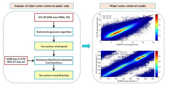
:The space-borne microwave radiometers and scatterometers can effectively measure global sea surface winds under non-precipitation. However, the measurements in rainy conditions significantly degrade, which are usually flagged as poor quality or invalidated for some scientific purposes. This paper develops a combined active–passive wind vector retrieval model for rainy conditions based on the HY-2B radiometer and scatterometer measurements. In our model, the polarization ratio of brightness temperatures at 6.925 GHz (PR06) is used as an indicator to implicitly represent the rain effect. For wind speed retrieval, a statistical regression model is trained as a function of PR06 and brightness temperatures of the radiometer. Moreover, two new geophysical model functions, including rain effect, are developed for wind direction inversion. Comparisons between HY-2B retrieval results and ERA5 wind products indicate that the retrieval model performs well under all rainy conditions. The overall root mean squared errors (RMSEs) of wind speed and direction retrievals are 1.60 m/s and 20.60°, respectively. With an increase in the rain rate, the wind retrieval performance degrades slightly and still provides a reliable retrieval result.
1. Introduction
Sea surface wind vectors make up an essential parameter in the ocean–atmosphere system. The measurement of sea surface winds is very important in understanding global climate change, exploring air–sea interactions, and improving extreme weather forecasts. Nowadays, the space-borne microwave scatterometers and radiometers are the main devices used to measure global sea surface wind vectors [1,2].
The microwave scatterometer measures sea surface wind by emitting microwave radiation and measuring its backscattering signal (the normalized radar cross-section) from the sea surface [3,4]. Under rain-free conditions, the measured backscattering signal strongly depends on surface wind speed, wind direction, azimuth angle, and incidence angle [5]. On the other hand, the microwave radiometer is a passive sensor measuring surface winds by observing the surface emission in terms of brightness temperature (TB), which is related to surface roughness, and thus to the wind speed [6,7]. Validations with buoy data and numerical weather prediction products have suggested that the rain-free retrieval algorithm can obtain the sea surface wind vector with an accuracy of about 1 m/s for passive radiometers [8], and less than 1.5 m/s and 16° for scatterometers [9]. However, the accuracy tends to degrade very rapidly when the rain occurs. A common perception is that the wind retrieval performance of the scatterometer degrades moderately under rainy conditions, but the measurements of the radiometer are unusable even in light precipitation. Rain mainly affects the microwave measurements by three mechanisms [10,11]. Firstly, rain can increase the atmospheric attenuation and thus decrease the signal-to-noise ratio of the measurements. Secondly, the rain drops can induce the rain volume backscatter, impacting the real measurements. Moreover, rain alters ocean surface roughness by the rain “splash” effect. The net effect of rain on microwave measurements depends on wind speed, rain rate, rain drops size distribution, and rain type. For these reasons, it is difficult to model the rain influence and distinguish the signal coming from rain and sea surface wind. This influence of rain leads to highly erroneous retrievals, invalid measurements, and less coverage of satellite wind measurements.
To quantitatively understand the microwave signal caused by rain, there are many studies focused on the effect of rain on radar backscattering and microwave emissivity from the ocean, including the scattering and emissivity mechanisms causing the signatures of rain [12,13,14,15]. For radar backscatter measurements, several wind/rain backscatter and attenuation models have been proposed to simultaneously retrieve the wind velocity and rain rate. When rain data are available, wind retrieval is performed by correcting the wind geophysical model functions. The wind/rain backscatter model is usually a function of wind speed, relative wind direction, incidence angle, rain rate, and other rain information (such as the distribution of rain drop sizes and rain height information) [11,16,17]. The main issue associated with this kind of model is the accurate rain information, which is cannot be obtained synchronously most of the time. Moreover, as a mitigating approach, some researches corrected rain effect on surface backscatter by simultaneously using passive measurements [12,18,19]. However, the retrieval performance of wind vector under rainy conditions is not ideal because the passive noise measurements from the scatterometer are noisy with large error. Unfortunately, only a few of satellites carried both the microwave scatterometer and radiometer, such as the Advanced Earth Observing Satellite-II and HY-2A, but most of them are terminated early or with less accuracy compared to passive measurements. For microwave radiometer measurements, Meissner and Wentz made the first attempt to retrieve accurate wind speed under rainy conditions using the WindSat radiometer with C-and X-band channel combinations to statistically reduce the influence of rain on brightness temperatures, but without decreasing the wind speed signal too much [15]. Recently, the algorithm was extended to apply to the measurements of tropical cyclone wind speed for the AMSR-2, AMSR-E, and WindSat radiometers [20,21]. Because the sensitivity of linearly polarized brightness temperature to wind direction is weak, multichannel radiometer usually cannot retrieve surface wind direction. Fortunately, to enhance the wind direction signal in linear polarization measurements, a modified second Stokes brightness AVH approach for rain-free conditions was proposed using a linear combination of H- and V-polarization brightness temperatures, which can mitigate the influence of the atmospheric state on brightness temperature and increase the dependence on sea surface wind direction [22,23,24,25,26]. The AVH method is favored to improve the retrieval performance of the wind direction.
The HY-2B satellite, which aimed to measure the sea surface temperature (SST) and the sea surface wind vector globally, was launched on October 2018, simultaneously carrying a conically scanning scatterometer operating on Ku band (13.256 GHz) and a multichannel scanning microwave radiometer operating on C, X, K, and Ka bands [27,28]. A comparison with buoy data and other sources of data indicates that both the two sensors have good performance in surface wind inversion in non-precipitation [28,29]. Therefore, HY-2B measurements provide an opportunity for us to study and correct the rain effect on active and passive measurements, and thus to retrieve the sea surface wind vector under rainy conditions. In this paper, we focus on developing the retrieval model using the active and passive HY-2B measurements, and testing its performance in sea surface wind inversion.
Our paper is organized as follows. Section 2 introduces the datasets used in model development and validation. Section 3 describes the new geophysical model functions (GMF) developed under rainy conditions and the active–passive retrieval method for wind vector retrieval. The model performance on ocean wind vector inversion is discussed in Section 4 by comparing HY-2B wind retrieval results with ECMWF ERA5 wind products. Section 5 concludes and summarizes our work.
2. Materials
We intend to develop a new wind retrieval model under rainy conditions and test its performance. The basis of such a study is the match-up datasets between HY-2B measured data, GPM rain data, ECMWF ERA5 wind vectors, and sea surface temperature products.
2.1. HY-2B Data
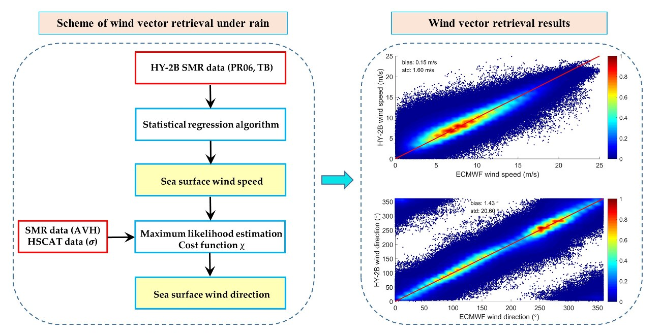
The brightness temperatures and the normalized radar cross-section , measured with SMR and HSCAT onboard HY-2B satellite, respectively, from 1 March 2019 to 31 May 2020, are used. We use the match-up dataset from 2019 to 29 February 2020 for training the rain–wind model and the residual data in 2020 to test the model and evaluate the wind retrieval performance. Data are provided by the Chinese National Satellite Ocean Application Service (NSOAS, https://osdds.nsoas.org.cn (accessed on 5 December 2020)). A histogram of the collocated GPM rain rate for HSCAT is shown in Figure 1. The matchups allow analysis of rain impact for rain rates up to about 100 km mm/h and most of the data ranging from 0.001 to 5 mm/h.
The SMR sensor is a conical-scanning microwave radiometer operating at 6.925, 10.7, 18.7, 23.8, and 37 GHz. Except for 23.8 GHz, with only vertical polarization measurement, other frequencies measure both the horizontal (H) and vertical (V) polarization brightness temperatures. In this paper, the SMR L2A 6.925 GHz, 10.7 GHz, 18.7 GHz, and 37 GHz brightness temperatures are spatially resampled to a resolution of 6.925 GHz using a Backus–Gilbert-type optimum interpolation scheme.
HY-2B HSCAT is a Ku-band (13.256 GHz) conically scanning scatterometer with an inner beam and an outer beam sweeping at an incidence angle of 41.5° and 48.6°, respectively. The inner beam operating at horizontal polarization generates a swath of about 1350 km. The outer beam operating at vertical polarization results in a swath of about 1750 km. The instrument specifications of SMR and HSCAT are listed in Table 1. The HSCAT backscatter measurements have an approximate original resolution of 25 km × 32 km and are reported on a 25 km × 25 km earth grid with L2A data. This 25 km × 25 km grid can be called a wind vector cell (WVC).
The time window of SCA and SMR is within about several seconds, which is effectively simultaneous. The spatial resolution of HSCAT and SMR data is different. To jointly use the active and passive data, the brightness temperatures are collocated into the HSCAT WVC grid via bilinear interpolation, since sea surface wind and other oceanic geophysical parameters are usually continuous. Moreover, because the ice can affect the SMR and HSCAT measurements, we only use the data for sea surface temperatures larger than zero degree Celsius and latitude ranging from 60° N to 60° S to avoid the ice influence. The number of the matchup under rainy conditions is approximately 200 million.
2.2. GPM IMERG_F Rain Data
To identify the HY-2B measurement data under rainy or rain-free conditions, accurate rain information is needed. The Global Precipitation Measurement (GPM) mission, consisting of an international network of satellites, can provide a new generation of global precipitation observations [30]. IMERG final run (IMERG_F) [31] is one of its various precipitation products at a high spatial and temporal resolution of 0.1° and 0.5 h, respectively. These data merge and interpolate several satellite microwave and infrared precipitation measurements. Moreover, monthly gauge data correction is applied in IMERG_F to reduce error and perform better accuracy. Here, the latest version (V06B) data are used by averaging rain data falling within the grid of HSCAT measurements. The IMERG_F rain data are available at https://gpm.nasa.gov/data/directory (accessed on 8 May 2021). The GPM rain rates are linearly interpolated in time and bilinearly interpolated in space to match up with the HY-2B SCA measurements.
2.3. ECMWF ERA5 Data
The European reanalysis 5 (ERA5) dataset produced by the European Centre for Medium-Range Weather Forecasts (ECMWF, https://www.ecmwf.int/ (accessed on 8 May 2021)) is used to build and train the new geophysical model functions and validate the retrieval results of ocean wind vector. In this paper, ERA5 0.25° gridded products, including sea surface temperature (SST), sea surface wind speed (WS), wind direction, are interpolated into the grid of HSCAT measurements temporally and spatially.
To clearly illustrate the datasets used in this paper, Table 2 summarizes all the data sets with the sources and downloads URLs.
3. Results
3.1. Geophysical Model Functions (GMFs)
3.1.1. Backscatter GMF under Rainy Conditions
Rain affects the measured of the scatterometer in three ways: (1) rain drops cause two-way attenuation along the wave propagation path, and thus reduce the transmission of radar signal, (2) rain drops increase the volume backscatter in the air, and (3) rain drops alter the roughness of the sea surface and affect the backscatter measured by the scatterometers. In general, the appearance of rain overestimates the surface wind speed when the rain volume backscatter effect dominates and underestimates rain attenuation in dominance. The backscatter measurements under rainy conditions can be expressed as a simple phenomenological form:
where is the backscatter measured by HSCAT, represents the surface backscatter caused by wind-induced roughness, is the surface backscatter from the raindrop splash effect, is the two-way rain attenuation, and is the volume scattering coming from rain drops in the air. Because rain-free geophysical model functions are very mature, we are only interested in the changed backscatter due to the rain. Theoretically, these three rain-related parameters are functions of the rain rate, rain height, and rain drop size, which usually are complicated. Moreover, it is difficult to distinguish the contribution of rain attenuation and surface backscatter caused by rain individually. For the sake of simplicity and independence on external rain information, we combine the rain effect into a lumped integrated parameter, and (1) simplifies to:
where represents all backscatter influence coming from rain. can be calculated using the existing GMF NSCAT-4 for rain-free conditions. The NSCAT-4 model [32] is a function of wind speed, wind direction, incidence angle, and azimuth direction, which has been applied and validated in several space-borne scatterometers. The input wind speeds and wind directions are obtained from the collocated ERA5 wind products, whereas the incidence angles and azimuth directions are provided by HSCAT L2A data. Thus, can be acquired by subtracting from the backscatter data measured by HSCAT ().
Previous researches have demonstrated that the linear polarization brightness temperatures are highly correlated with the atmospheric precipitation environment [33]. To model without rain information as the input, a parameter based on brightness temperatures is required to represent the rain effect. The parameter is possible due to the difference of frequency and polarization in the sensitivity of TB to the rain effect. Generally, the TB at vertical polarization is insensitive to ocean surface wind speed but sensitive to rain, whereas the horizontally polarized TB is sensitive to both wind speed and rain [12]. Our correlation analysis suggests that the rain backscatter correlates with the surface wind speed, the relative wind direction, and the polarization ratios (PRs) of brightness temperature at different frequencies. Therefore, can be modeled as .
where ,, and are the coefficients that are related to wind speed and the polarization ratio of brightness temperature (where and represent the brightness temperature at horizontal and vertical polarization, respectively). is the relative wind direction (RWD) defined as the difference of the SMR scanning azimuth angle and wind direction. The matchup data and regression analysis are used to obtain the c coefficients for different wind speeds and PR values.
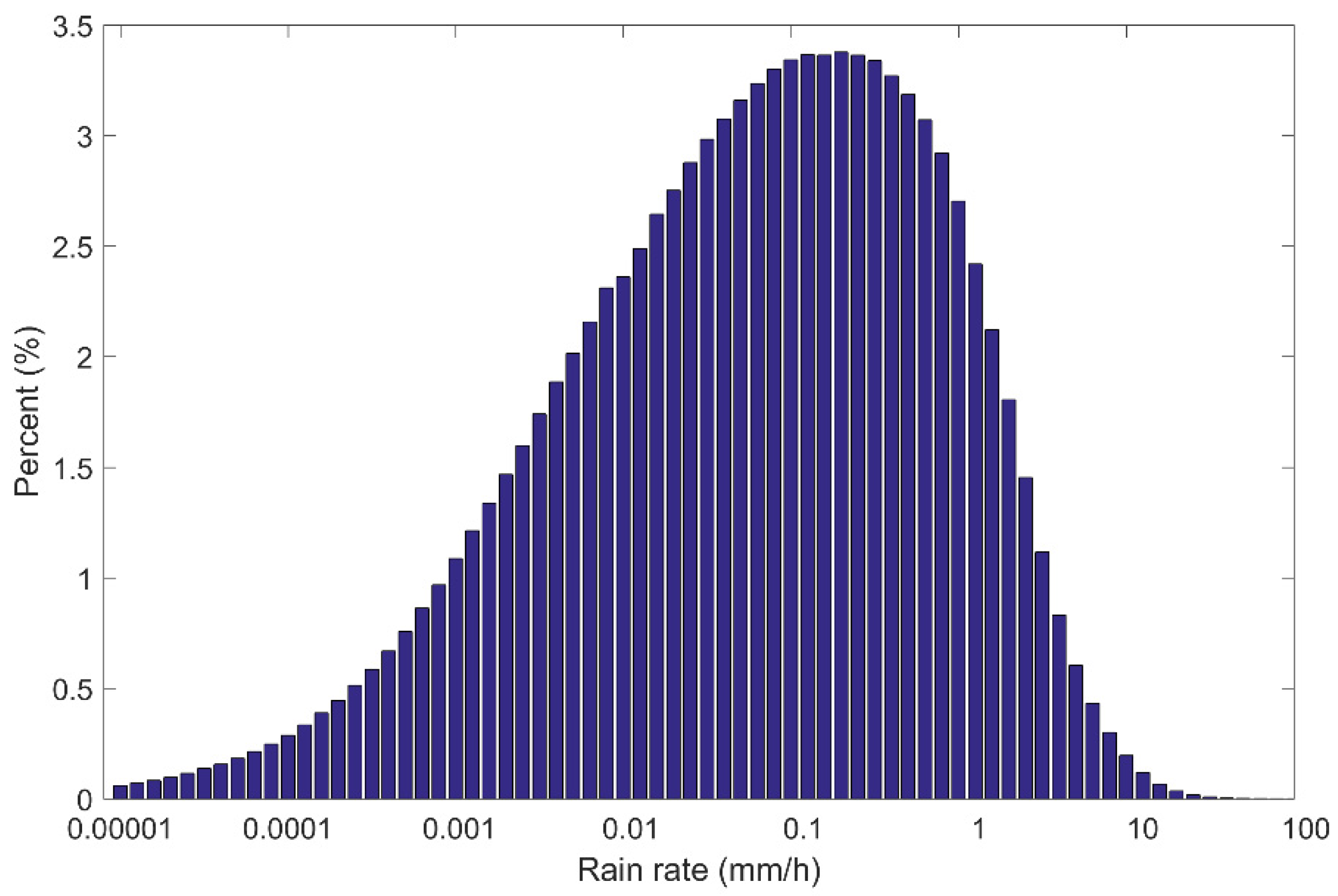
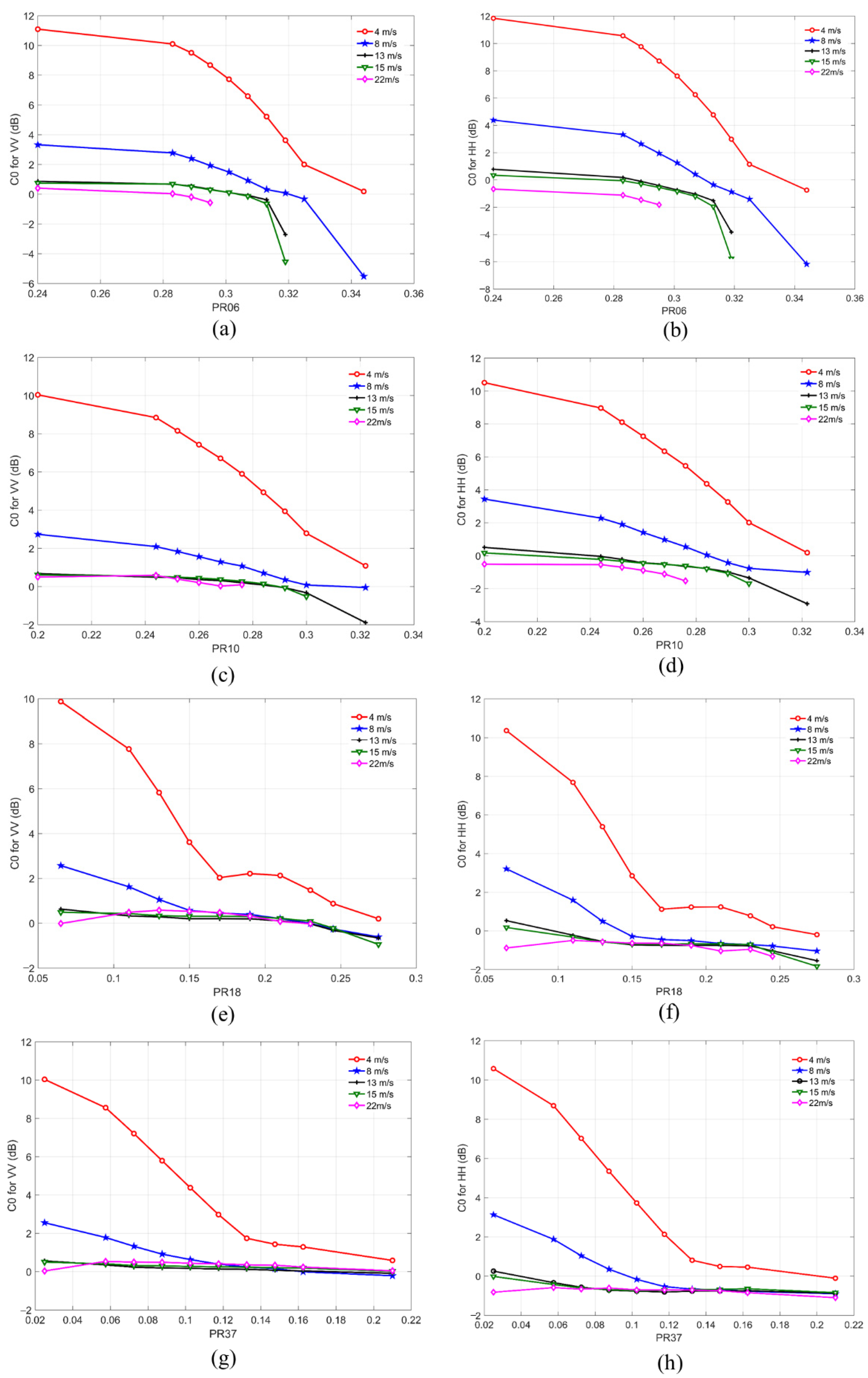
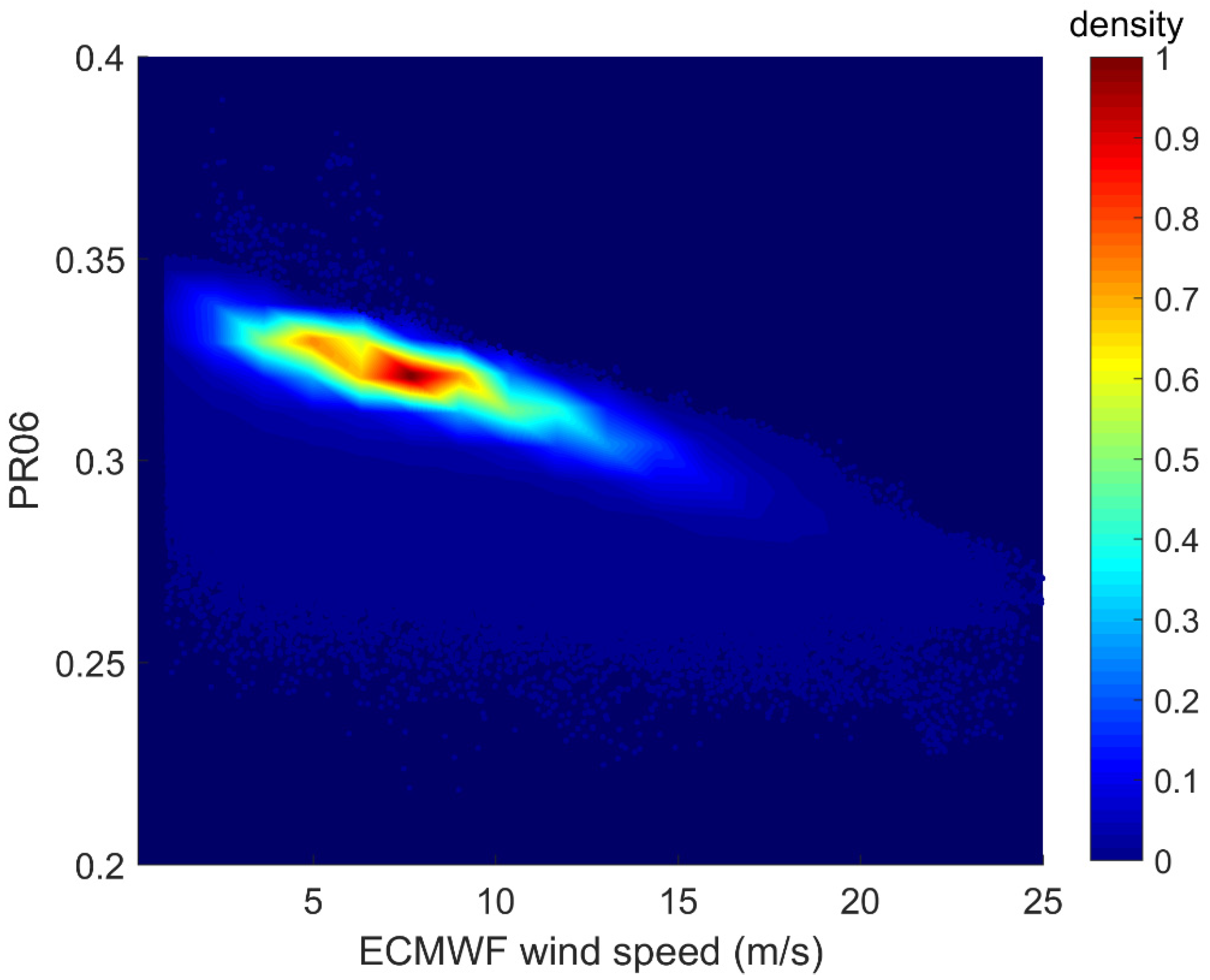
Figure 2 presents the relationship between the coefficient and the PR at 6.925 GHz (PR06), 10.7 GHz (PR10), 18.7 GHz (PR18), and 37 GHz (PR37) for different wind speeds. The left column is for VV polarization and the right column is for HH polarization. It is seen that is more sensitive to PR06 than PR10, PR18, and PR37, especially for low wind speeds where rain severely affects the measurements. The sensitivity reflects the PR dependence of . We want to find a parameter to express the rain effect, whereby the parameter with a strong dependency is desired. Therefore, the PR06 is selected to implicitly account for the rain effect on backscatter measurements, and is used to fit the coefficients ,, and. The absolute value of at HH polarization is larger a little than that at VV polarization, which implies that the HH measurements are easily affected by the rain. Furthermore, it is obvious that decreases gradually alongside an increase in wind speed and tends to be insensitive at high wind speed. For a wind speed of 4 m/s, the rain backscatter can be up to 12 dB at low PR06, while the absolute values for a high wind speed of 22 m/s are less than 2 dB. The coefficient reflects the net effect of rain on surface backscatter. For low wind speed and low PR06, the changed backscatter due to rain is positive, while the net effect is usually negative for high wind speed and high PR06. Here, it is worth noting that some data are missing for the high wind speed curves in Figure 2 because PR is usually small at high wind speeds, and there is no match-up data for high wind speeds and high PR values, as shown in Figure 3 for example. The color scale in the figure represents the density of data, with the reddest color indicating the maximum density.
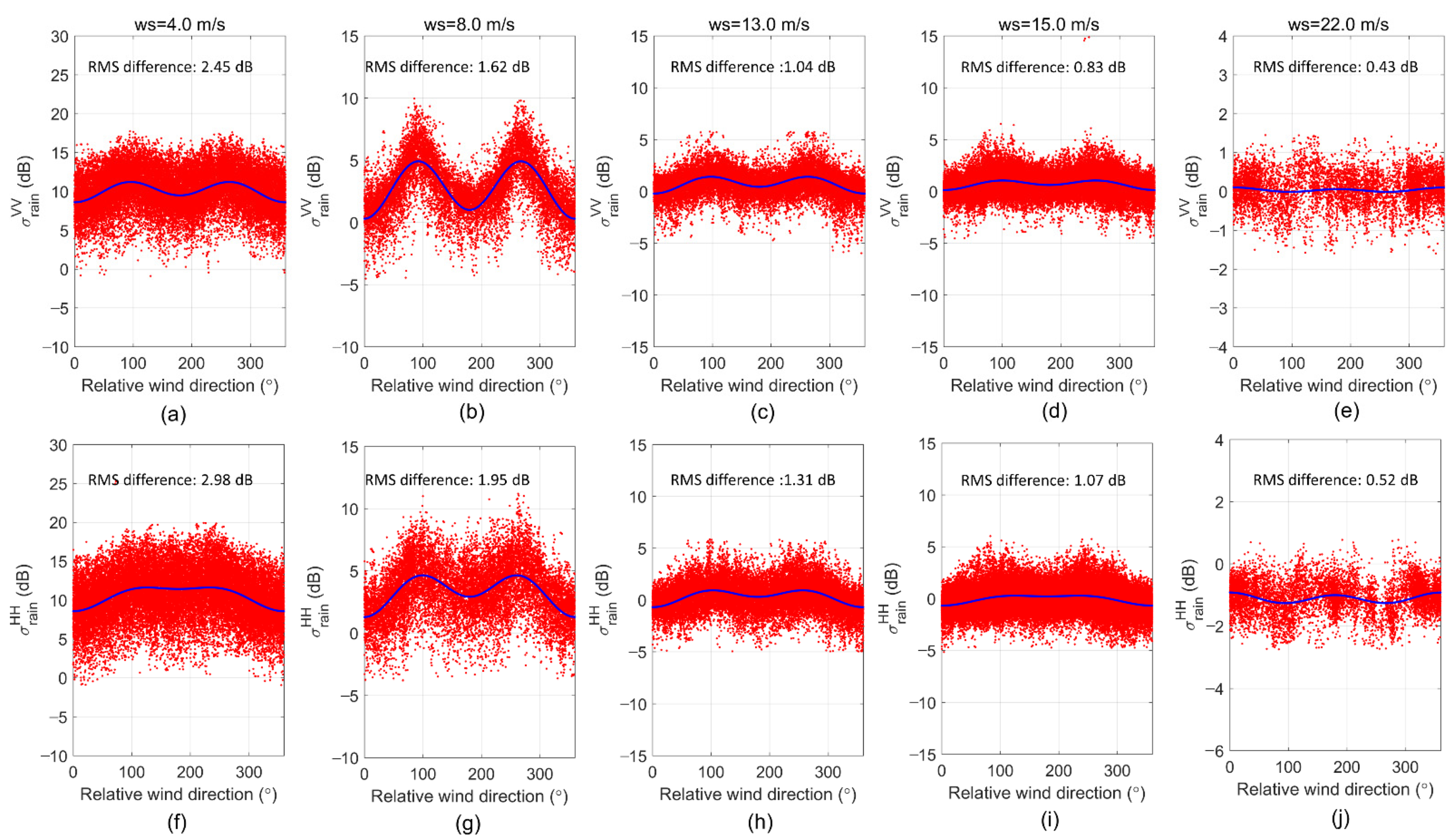
Figure 4 shows the sample GMF regression fits versus the relative wind direction for both polarizations at different wind speeds, in which the PR06 ranges from 0.280 to 0.286. To validate the fits, the measured data in Figure 4 are taken from the testing dataset. Visually, the rain backscatter model follows the data very well. There are several statistical techniques for analyzing the estimation uncertainty of a model [34,35,36]. Here, we quantify the fitting performance using the root mean squared (RMS) difference between the measured data and the fitting results. The RMS differences are shown in each panel indicate that the fitting performance is better at a high wind speed than that at a low wind speed. One possible reason is the low signal-to-noise ratio of SCA backscatter measurements at low wind speeds. Furthermore, there is a clear dependence of on the relative wind direction for wind speeds lower than 13 m/s, with the peak-to-peak variations of about 3.5 dB, 3.3 dB, and 1.5 dB at 4 m/s, 8 m/s, and 13 m/s for HH polarization, respectively, and about 3.0 dB, 4.6 dB, and 1.7 dB for VV polarization, respectively. With an increase in the wind speed, the directional harmonics become weak. The phenomenon of wind directional dependence confirms that the striking interaction of rain drops to the sea surface, including rings, stalks, turbulences, and crowns, can obviously alter the wind-induced capillary wave field, especially for a low wind speed. After obtaining these coefficients, a new GMF used to retrieve wind vector under rainy condition can be established:
where represents the NSCAT-4 model.
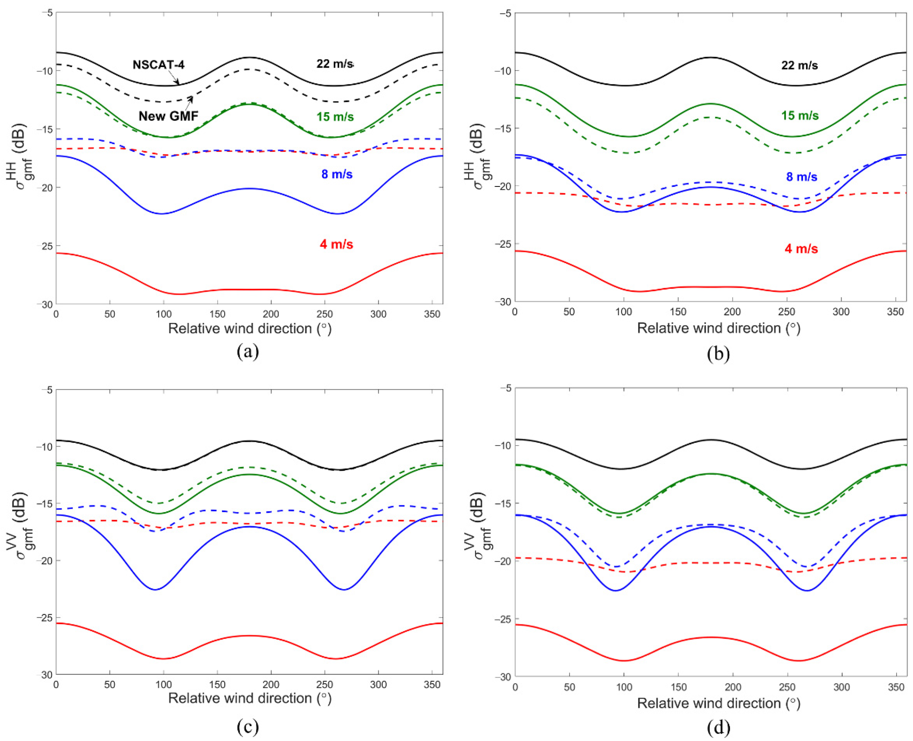
Several examples of the new GMF are shown in Figure 5 for four wind speeds and two values of PR06. To compare with the GMF for rain-free conditions, the corresponding results estimated from NSCAT-4 are also displayed. It is apparent that rain suppresses the wind/backscatter directional dependence for low wind speeds. The directional dependence remains for wind speeds larger than 8 m/s, suggesting the possibility of wind direction retrieval under rainy conditions.
To effectively understand the performance of the new GMF, the RMS differences between model results and backscatter measurements are calculated for different wind speeds and PR06 values, and listed in Table 3. Since the GMF will be used for wind direction retrieval in the next section, the peak-to-peak values of the backscatter with wind direction are also estimated and given in Table 3. The peak-to-peak value can reflect the sensitivity of surface backscatter to wind direction. It is seen that the RMS differences are larger than the peak-to-peak values when the wind speed is below 8 m/s, which infers that the estimation uncertainty of the model is large, and the wind direction signal is too small to be retrieved at low wind speed. With an increase in the wind speed, the wind direction dependence becomes stronger, larger than the model uncertainty, which makes it possible to retrieve wind direction at high wind speeds under rainy conditions.
3.1.2. AVH Model Function under Rainy Conditions
By enhancing the wind directional signal in linear polarization brightness temperature with a passive microwave radiometer, Meissner and Wentz proposed a technique using a modified second Stokes brightness AVH approach [22,23]. The AVH is defined as a linear combination of H and V polarization brightness temperatures [24].
For SMR frequencies, especially for lower frequencies, the atmospheric transmission is usually large, and then the parameter A can be simply expressed as follows.
where and are the brightness temperatures at H and V polarization, and SST is the sea surface temperature in Kelvins. This linear combination can mitigate the influence of the atmospheric state and may depend on the sea surface temperature, sea surface wind speed, and direction. The application of AVH in inversion of wind direction under rain-free conditions has been successfully conducted. To improve the retrieval performance of wind direction under rainy conditions, we expect that the AVH method can be used to help retrieve wind direction under rainy conditions by combining the HSCAT backscatter measurements. Given the measured H and V polarization brightness temperature, and the corresponding sea surface temperature, the at different frequencies can be derived.
Referring to [24], the geophysical model function of AVH can be expressed as follows:
where ,, and are the coefficients that are related to wind speed and sea surface temperature, and is the relative wind direction. describes the isotropic property, and the and terms represent the wind direction dependence. Since the brightness temperatures of 37 GHz are easily affected by atmospheric state and are attenuated severally under rainy conditions, we do not take account for the AVH at 37 GHz in wind inversion.
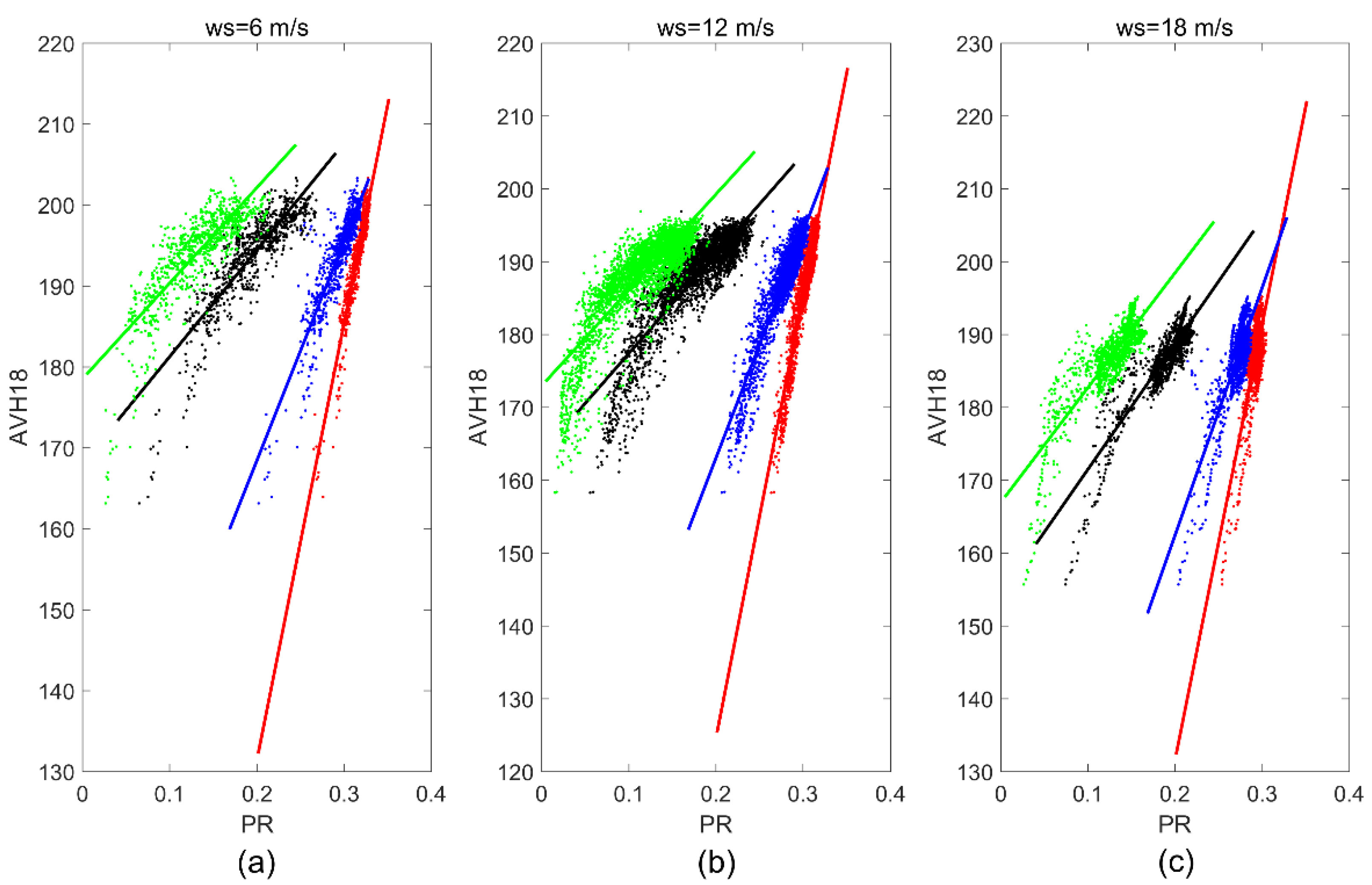
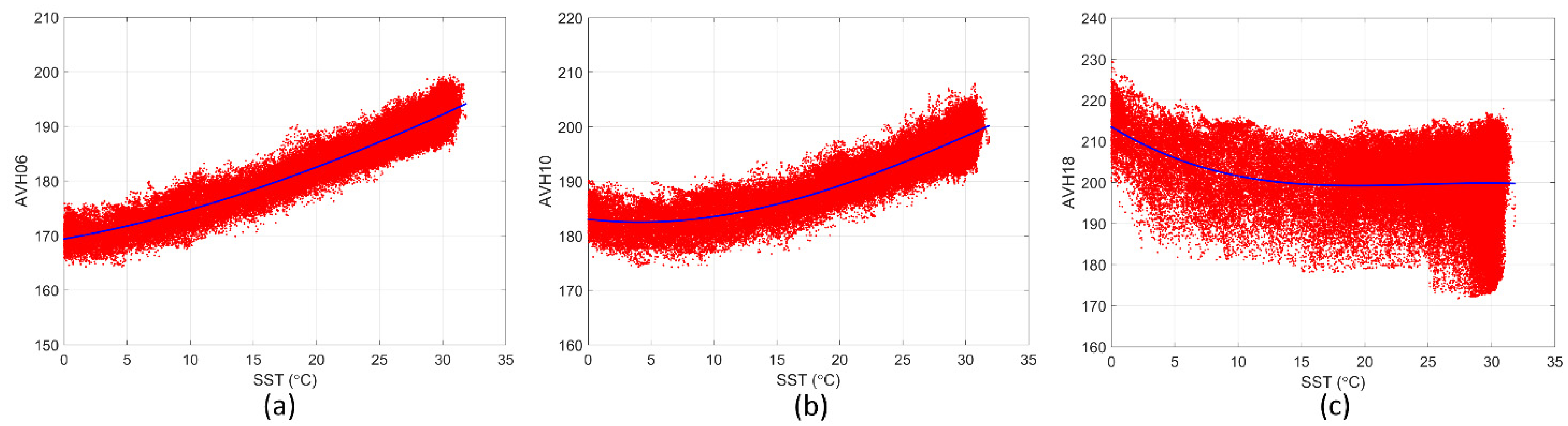
From the analysis results in the previous section, it is known that the PR of brightness temperature is a good indicator to implicitly describe the rain impact on backscatter measurements. Due to the suppression of the AVH approach to atmospheric affection and the strong penetration of C and X bands, we find that the AVH variations of C and X bands with PR06, PR10, PR18, and PR37 are similar and small, but the change in AVH at 18.7 GHz versus PR06 is obvious. For the constant SST of 15 °C and the relative wind direction of 45°, Figure 6 presents an AVH of 18.7 GHz (AVH18) versus a PR value for wind speeds at 6 m/s, 12 m/s, and 18 m/s, respectively, whereby red, blue, black, and green represent the AVH18 versus PR06, RR10, PR18, and PR37, respectively. Furthermore, the scatters are the AVH measurements acquired from SMR brightness temperatures, and the solid lines denote the corresponding fitting curves. Obviously, AVH18 under rainy conditions varies faster with PR06 than with PR10, PR18, and PR37, sequentially. Therefore, in addition to wind speed, wind direction, and SST, PR06 is required in the development of the AVH model under rainy conditions. Based on the match-up data, we analyzed the relationship of wind directional dependence of AVH versus wind speed, SST, as well as PR06. Compared to wind speed, the modulation of SST and PR06 to wind direction dependence can be neglected, which allows us to model the AVH as:
where is only the function of SST; , , and are the functions of wind speed; and relates to PR06 and wind speed.
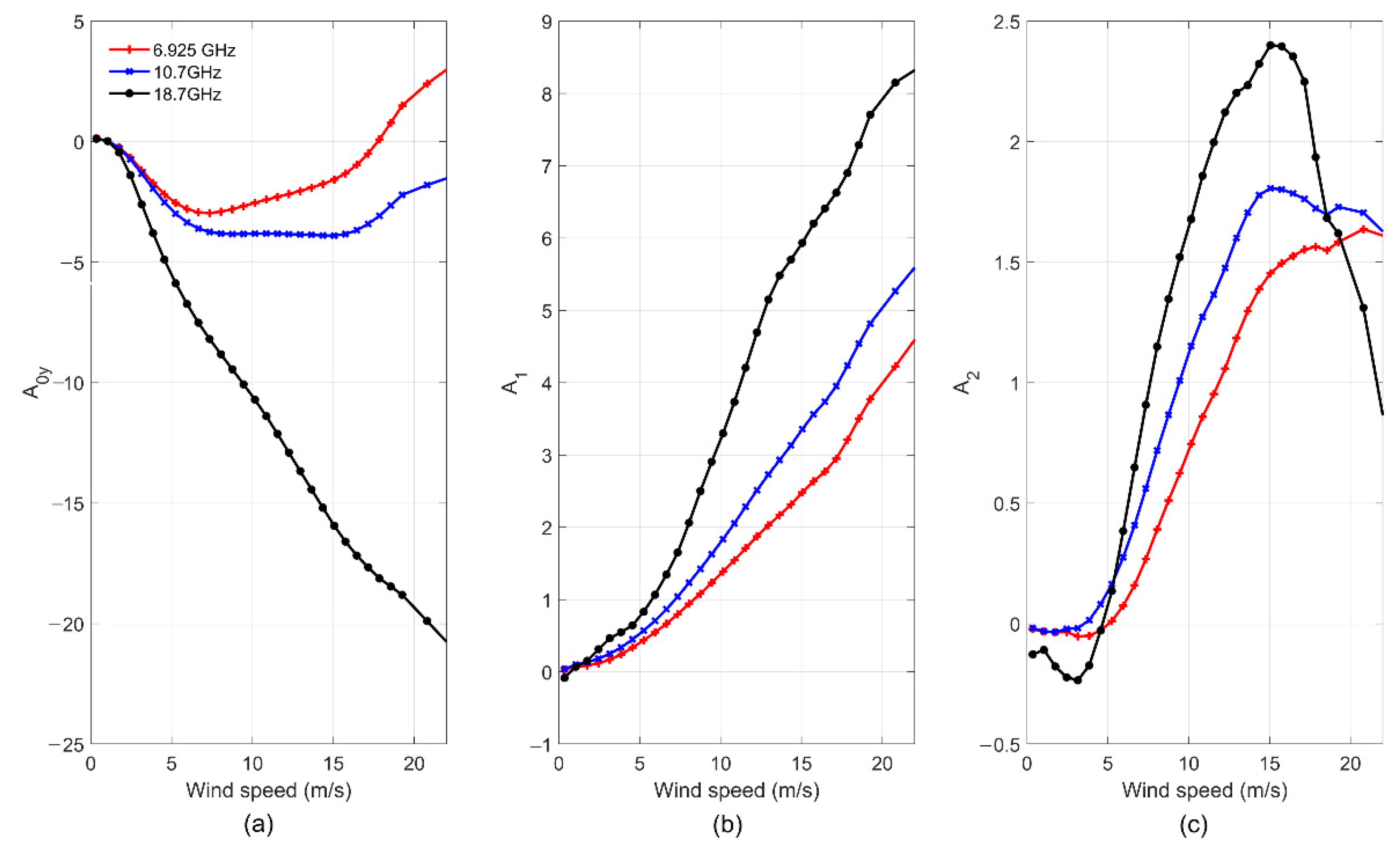
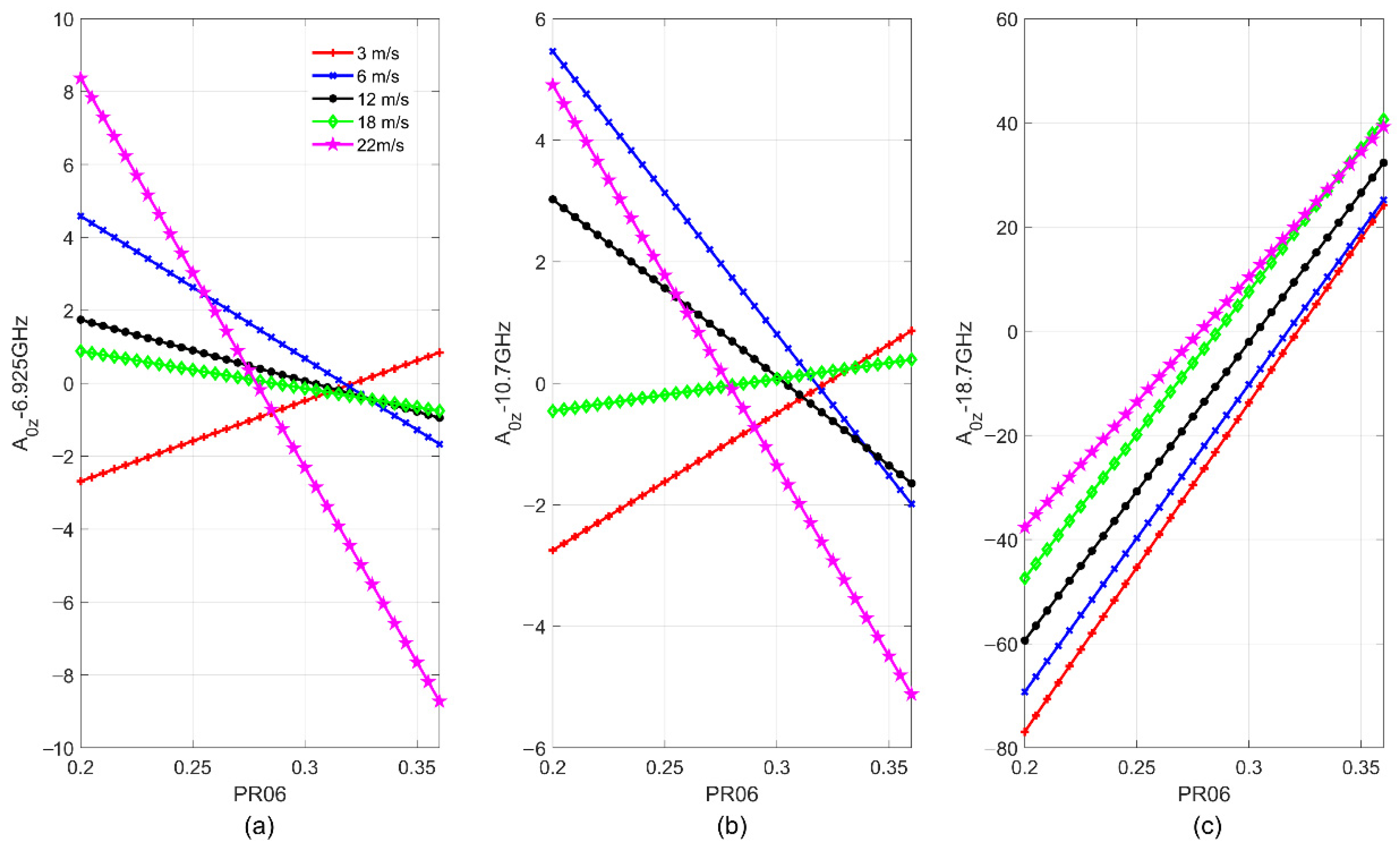
Next, the procedure of deriving the function coefficients is described, and the coefficients are provided. Firstly, we acquire the coefficient by assuming the surface is smooth to eliminate the contribution of wind speed and wind direction approximately, where the matched wind speeds are less than 1 m/s. Then, we can obtain the overall fitting tends of AVH versus SST via regression analysis. The contribution of PR06 is not considered by fitting on all PR06s. Figure 7 shows the dependence of AVH on SST for three frequencies, in which the blue solid lines represent the corresponding fitting curves at each frequency. The AVH18 measurements varying with SST are more scattered than other two frequencies, which infers that the rain correction is required at a high frequency. Secondly, using function and subtracting its results from the measurements of AVH, we can derive the , , and coefficients via a linear regression method, and the results are shown in Figure 8. Finally, subtracting the results estimated by and from the AVH measurements allows us to obtain the function of the coefficient, which is derived by linear fitting PR06 at various wind speeds. Figure 9 presents the coefficients versus PR06 at 6.925 GHz, 10.7 GHz, and 18.7 GHz, respectively. The PR06 dependence is very strong for high frequency, with the dynamic range of larger than 80 K approximately at 18.7 GHz. The dependence at low frequencies is relatively small, but still cannot be neglected. Figure 8 and Figure 9 indicate that the AVH at high frequency is very sensitive to wind vector and rain effect; thus, if we can model the contribution of wind vector and rain well, AVH is very helpful to retrieve the sea surface wind vector under rainy conditions.
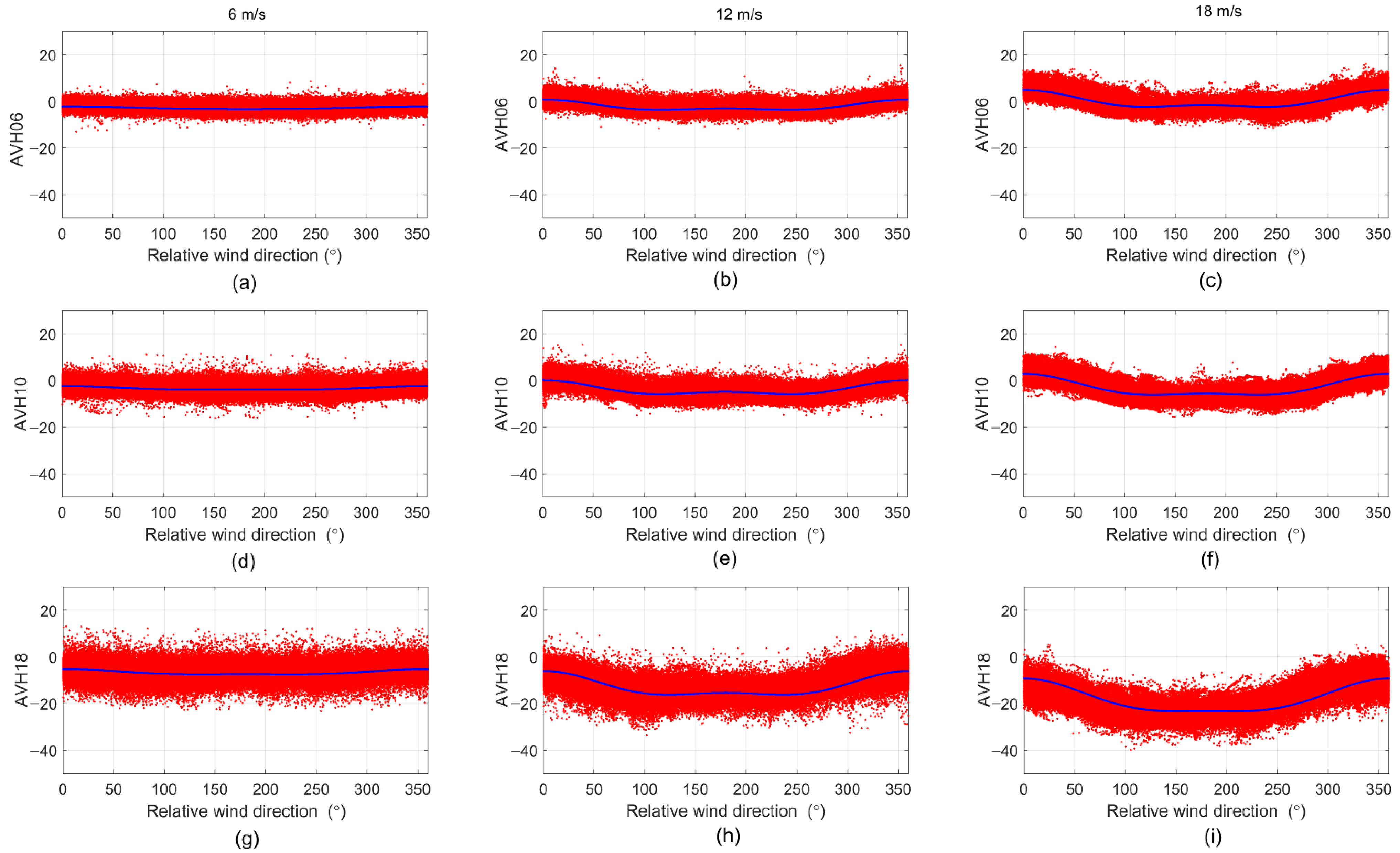
To clearly illustrate the wind directional dependence, the AVH measurements after subtracting the estimates of and , the corresponding fitting results calculated from function varying with relative wind direction are presented in Figure 10 for wind speeds at 6 m/s, 12 m/s, and 18 m/s, respectively. The first, middle, and last row is for 6.925 GHz (AVH06), 10.7 GHz (AVH10), and 18.7 GHz (AVH18), respectively. The AVH measurements and the model results are in good agreement for all wind speeds. Compared to the wind directional dependence at a high frequency, the variation of AVH at a low frequency is smaller, and the scatter of the AVH points (i.e., the geophysical noise) is smaller, mainly due to the reduced impact from the rain. Moreover, similar with the results under rain-free conditions [24], for low wind speeds, the AVH anisotropy is weak and almost comparable with the geophysical noise of the model, and the dynamic ranges at 6 m/s are about 1.0, 1.5, and 2.2 K for the three frequencies, respectively, which makes it difficult to only use passive measurements for wind direction retrieval. For high wind speeds, the anisotropy caused by surface wind direction is improved, with a peak-to-peak value of about 4.4 K, 6.0 K, and 10.2 K for wind speed at 12 m/s, and about 7.2 K, 9.0 K, and 13.8 K for 18 m/s, respectively. Thus, it is possible to obtain good wind direction retrievals at a high wind speed.
3.2. Wind Vector Retrieval Model
3.2.1. Statistical Linear Regression for Wind Speed
The strong impact of rain on backscatter measurements makes it difficult to retrieve wind speed at a low wind speed using scatterometer measurements. Fortunately, the combination of the measurements from SMR at multiple frequencies can mitigate the rain contamination since the lower frequencies have relatively small atmospheric attenuation and scattering [15,20,21]. The spectral differences of brightness temperature are different for wind-induced surface emissivity and the rain-induced contribution. Therefore, the combinations between the C- and X-band channels have been successfully used in wind speed inversion under rainy conditions because they are insensitive to rain but sensitive to wind speed. Based on this principle, we retrieve wind speed under rainy conditions with a similar regression form proposed in [20]. Differently, we replace the parameter of rain rate with PR06 to avoid the reliance on external rain information. Thus, the regression has the following form:
In the expression, the index i represents the frequency and runs over C and X bands in the sum, the index represents the polarization of H-pol and V-pol, and is the corresponding brightness temperature measured by SMR. We train ten models for ten different PR06 intervals based on the PR06 distribution. The coefficients are listed in Table 4.
Note that the superscript in and coefficients denotes frequency and polarization.
3.2.2. Wind Direction Retrieval Model
The sea surface wind direction retrieval is based on the backscatter measurements of HSCAT and the passive AVH measurements from SMR. The retrieval is performed by minimizing the following cost function , consisting of the residues between measurements and model results, as shown in (11).
where represents the number of the HSCAT measured data in each WVC, and represents the three SMR frequencies. and are the corresponding variance measurements. can be acquired from the HSCAT L2B data file. is determined by the comparison of measurements data and the results calculated from the model; 1.5 K, 1.8 K, and 2.5 K correlate with 6.925 GHz, 10.7 GHz, and 18.7 GHz, respectively. Note that the wind speed inputs to the geophysical model functions in Equation (11) are from the statistical regression results in Section 3.2.1. In the minimization procedure, the solutions of wind direction can be searched. Because the dependence of on wind direction is bi-harmonic, a set of 2 to 6 possible resolutions can be obtained. The median-filter-based ambiguity removal algorithm introduced in [37] is used to select the best wind direction from several ambiguous results.
4. Discussion
Taking ocean wind measurements using satellite microwave instruments under rainy conditions has long represented a challenging problem. Sea surface wind retrieval algorithms for rain-free conditions are effective but degrade very quickly when precipitation occurs. For many applications such as weather forecasting, accurate wind retrievals under rainy conditions is highly desirable. In the above section, based on HY-2B satellite measurements, we developed a combined active–passive wind retrieval model for rainy conditions. The major difference from previous studies is that we use the polarization ratio of C-band (PR06) rather than the rainfall rate to implicitly account for the rain effect on sea surface backscatter and passive measurements. Validating the developed geophysical model functions demonstrates that the PR06 can effectively characterize the rain effect. Next, we will discuss the retrieval performance of the developed model.
The active–passive models for wind vector retrieval under rainy conditions are tested with the testing matchups, which are not used for the model training. The retrieval results are compared to the collocated ECMWF ERA5 wind products. The overall root mean squared errors of their differences under all rainy conditions are estimated, approximately 1.60 m/s and 20.6° for wind speed and direction, respectively. The corresponding mean biases are 0.15 m/s and 1.43°, respectively.
Figure 11 shows the density scatterplots of HY-2B wind retrievals versus the collocated ECMWF ERA5 wind vectors in three different rain rate regimes. The first row is for wind speed retrieval, and the second row is for wind direction retrieval. The color scale represents the density of the comparison data—the redder the color, the greater the data density. Overall, good agreement can be seen between the HY-2B wind vectors and the ECMWF winds. The statistical results for mean bias and standard deviation listed in each panel also suggest that the retrieval model performs well under all rainy conditions. In light rain (<4 mm/h), where most of the matchup datasets are located, the standard deviation of wind speed and direction is 1.55 m/s and 20.51°, respectively, and the mean biases are small. Moreover, compared to the results in moderate and heavy rain, the comparison data seem more scattered, but the percentage of those retrievals with large errors is low actually, i.e., only about 4% for the absolute value of the difference between the HY-2B wind vector and ERA5 for data larger than 5 m/s and 50°. After excluding these retrievals with large errors, the standard deviation of wind speed and wind direction retrievals reduce to 1.40 m/s and 15.88°, respectively. With an increase in the rain rate, the wind direction retrieval performance keeps stable with a constant standard deviation of near 21° and does not significantly decrease even in heavy rain. On the other hand, the wind speed retrieval degrades slightly with increasing rain rate, but nevertheless still provides a reliable result in heavy rain, with an RMS difference of about 2.9 m/s. In heavy rain, the small signal-to-noise ratio of the passive measurements and the strong atmospheric scattering by rain lead to the large wind speed retrieval errors. The above statistical results demonstrate the capability of the active–passive wind retrieval model to retrieve usable and realistic sea surface wind vectors under rainy conditions.
In the procedure of developing the retrieval model, it is implied that the rain impact on wind inversion is more severe for low wind speeds. Here, we calculated the RMS errors of the retrievals for wind speeds below and above 8 m/s, respectively. The RMS errors for wind speed retrievals are 1.81 m/s and 1.39 m/s, and those for wind direction retrievals are 27.26° and 12.31°, respectively, which indicates that this is indeed the case. To better illustrate the results, Figure 12 displays the RMS errors of wind speed and wind direction as a function of wind speed, which is estimated from wind speed bins with a bin width of 2 m/s. As expected, the performance of the model degrades with reducing wind speeds. For wind speeds lower than 4 m/s, the wind retrieval error is large, up to near 38° and 3.1 m/s for wind speed and direction, respectively. Then, following an increase in the wind speed, the RMS error of wind direction retrievals decreases gradually until the wind speed exceeds 17 m/s. On the other hand, the wind speed retrieval performs best at the wind speed of about 10 m/s, and then tends to degrade approximately linearly as the wind speed increases. These results indicate that the rain effects on wind vector retrievals are not only related with the rainfall intensity, but also with the wind speed.
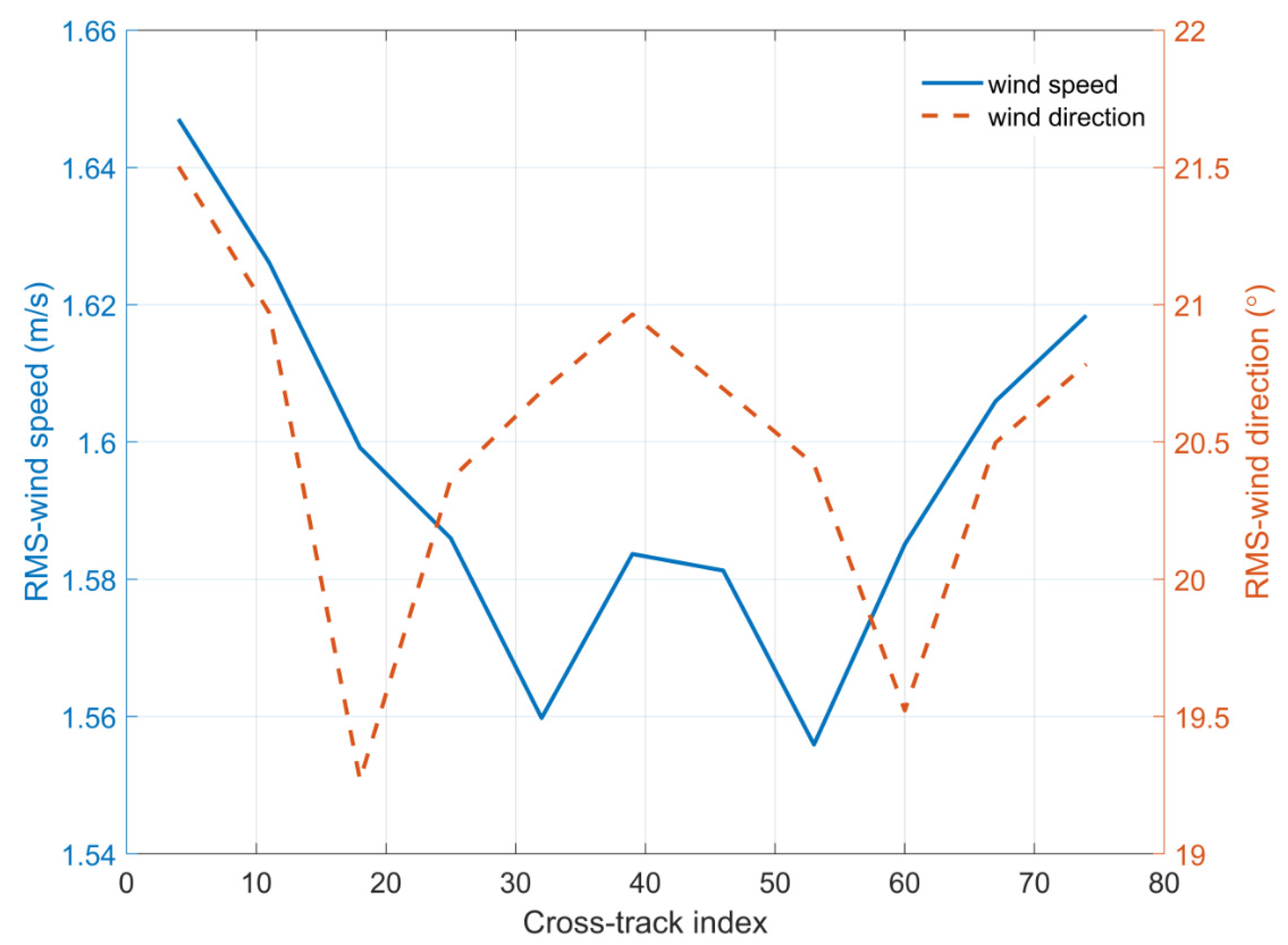
Moreover, under rain-free conditions, the wind vector retrievals from the conical-scanning type of scatterometer suffer some degradation in near nadir- and outer-swath region due to the poor diversity of observing azimuth angles [9]. Figure 13 presents the RMS differences between ECMWF winds and our retrieval results as a function of the cross-track WVC index. The WVCs with an index ranging from 1 to 38 are in the left swath, while those with an index ranging from 39 to 76 are in the right swath. Both the RMS curves of wind speed and wind direction exhibit the obvious shape of “W” with cross-track index, which is similar with those results in rain-free conditions.
This study provides an approach to retrieve sea surface wind speed and wind direction under rainy conditions for wind speeds below 22 m/s, and its retrieval results are reliable and usable.
5. Conclusions
In this paper, we focused on developing an active–passive wind retrieval model under rainy conditions based on HY-2B measurements and tested this model by comparing its retrieval results with the collocated ECMWF wind products.
The active–passive model is based on the difference of frequency and polarization in the sensitivity of brightness temperatures to rain effect, which makes it possible to find a parameter from brightness temperatures at different polarizations as the indicator to represent the rain effect on microwave measurements. Our analysis suggests that the polarization ratio of the linear polarization brightness temperatures at low frequency is sensitive to the rain effect. Therefore, the polarization ratio at 6.925 GHz (PR06) is included in our new geophysical model functions and our statistical regression model to implicitly consider the rain effects.
The wind speed and wind direction are retrieved separately. For wind speed retrieval, we follow the previous model proposed by Meissner and Wentz [15], which suggests that the combinations between the C- and X-band channels are useful in wind speed inversion under rainy conditions because they are insensitive to rain but sensitive to wind speed. In order to avoid relying on the external rain rate data, we replace the rain rate in the model with PR06. In wind direction inversion, in addition to using the HSCAT Ku-band backscatter measurements, we also utilize the combinations of brightness temperatures at C, X, and K bands, i.e., AVH, to help retrieve wind direction, since the AVH can enhance the wind direction signal and mitigate the atmospheric influence.
This study demonstrates the procedure of developing the new model functions for the HSCAT backscatter and SMR AVH which are used in wind direction inversion, and presents how to train a wind speed retrieval model under rainy conditions from the match-up datasets. Moreover, by utilizing the testing dataset, we retrieved sea surface wind vectors based on this active–passive wind retrieval model under rainy conditions and compared the results with the collocated ECMWF wind products. The comparisons show that the model performs very well both with light and heavy rain, with an overall retrieval RMS error of about 1.60 m/s and 20.6° for wind speed and wind direction, respectively. The wind vector accuracy degrades lightly with increasing rain, with wind speed ranging from about 1.55 m/s in light rain to 2.67 m/s in heavy rain, and from about 20.51° to 21.32° for wind direction.
In future, the model can be further improved using resolution enhancement of SMR measurements to reduce the sampling mismatch error between SMR and HSCAT data due to the different footprint. It is also desired that the retrieval model can be extended to tropical cyclones wind retrievals and other sensors.
Author Contributions
Conceptualization, S.L.; methodology, S.L. and Y.L.; software, S.L. and X.Y.; validation, S.L. and W.Z.; formal analysis, S.L., A.L.; investigation, S.L., X.J. and X.Y.; resources, S.L.; data curation, S.L. and Y.L.; writing—original draft preparation, S.L.; writing—review and editing, S.L. and Y.L.; visualization, S.L. and A.L.; supervision, H.D.; project administration, H.D. All authors have read and agreed to the published version of the manuscript.
Funding
This research received no external funding.
Data Availability Statement
The HY-2B HSCAT and SMR L2A data are available at NSOAS (https://osdds.nsoas.org.cn/ (accessed on 5 December 2020)). The GPM IMERG_F rain data are publicly available at https://gpm.nasa.gov/data/directory (accessed on 8 May 2021). The ECMWF ERA5 data are distributed at https://www.ecmwf.int/ (accessed on 8 May 2021).
Acknowledgments
We would like to thank Hao Li, Xiaoning Wang, Lixia Liu, and Yantao Huo for their helpful discussions.
Conflicts of Interest
The authors declare no conflict of interest.
References
- Vogelzang, J.; Stoffelen, A. Scatterometer wind vector products for application in meteorology and oceanography. J. Sea Res. 2012, 74, 16–25. [Google Scholar] [CrossRef]
- Yueh, S.H.; Wilson, W.J.; Li, F.K.; Nghiem, S.V.; Ricketts, W.B. Polarimetric measurements of sea surface brightness temperatures using an aircraft K-band radiometer. IEEE Trans. Geosci. Remote Sens. 1995, 33, 85–92. [Google Scholar] [CrossRef]
- Jones, W.L.; Schroefer, L.C.; Boggs, D.H.; Bracalente, E.M.; Brown, R.A.; Dome, G.J.; Pierson, W.J.; Wentz, F.J. The SEASAT-A satellite scatterometer: The geophysical evaluation of remotely sensed wind vectors over the ocean. J. Geophys. Res. 1982, 87, 3297–3317. [Google Scholar] [CrossRef]
- Liu, S.; Wei, E.; Jin, X.; Lv, A.; Dang, H. The performance of dual-frequency polarimetric scatterometer in sea surface wind retrieval. J. Ocean Univ. China 2019, 18, 1051–1060. [Google Scholar] [CrossRef]
- Wentz, F.J.; Smith, D.K. A model function for the ocean-normalized radar cross section at 14 GHz derived from NSCAT observations: NSCAT validation and science. J. Geophys. Res. 1999, 104, 11499–11514. [Google Scholar] [CrossRef]
- Brown, S.T.; Ruf, C.S.; Lyzenga, D.R. An emissivity-based wind vector retrieval algorithm for the WindSat polarimetric radiometer. IEEE Trans. Geosci. Remote Sens. 2006, 44, 611–621. [Google Scholar] [CrossRef]
- Liu, S.B.; Cui, X.D.; Li, Y.N.; Jin, X.; Zhou, W.; Dang, H.X.; Li, H. Retrieval of sea surface temperature from the scanning microwave radiometer aboard HY-2B. Int. J. Remote Sens. 2021, 42, 4621–4643. [Google Scholar] [CrossRef]
- Bettenhausen, M.H.; Smith, C.K.; Bevilacqua, R.M.; Wang, N.-Y.; Gaiser, P.W.; Cox, S. A nonlinear optimization algorithm for WindSat wind vector retrievals. IEEE Trans. Geosci. Remote Sens. 2006, 44, 597–610. [Google Scholar] [CrossRef]
- Wang, Z.; Stoffelen, A.; Zou, J.; Lin, W.; Verhoef, A.; Zhang, Y.; He, Y.; Lin, M. Validation of new sea surface wind products from scatterometers Onboard the HY-2B and MetOp-C satellites. IEEE Trans. Geosci. Remote Sens. 2020, 58, 4387–4394. [Google Scholar] [CrossRef]
- Ulaby, F.T.; Moore, R.K.; Fung, A.K. Microwave Remote Sensing: Active and Passive. Volume II: Radar Remote Sensing and Surface Scattering and Emission Theory; Addison-Wesley: Boston, MA, USA, 1982. [Google Scholar]
- Nie, C.; Long, D.G. A C-band wind/rain backscatter model. IEEE Trans. Geosci. Remote Sens. 2007, 45, 621–631. [Google Scholar] [CrossRef]
- Gohil, B.S.; Sikhakolli, R.; Gangwar, R.K.; Kiran Kumar, A.S. Oceanic rain flagging using radar backscatter and noise measurements from Oceansat-2 scatterometer. IEEE Trans. Geosc. Remote Sens. 2016, 54, 2050–2055. [Google Scholar] [CrossRef]
- Zhang, G.; Li, X.; Perrie, W.; Zhang, B.; Wang, L. Rain effects on the hurricane observations over the ocean by C-band Synthetic Aperture Radar. J. Geophys. Res. Ocean. 2016, 121, 14–26. [Google Scholar] [CrossRef] [Green Version]
- Amarin, R.A.; Jones, W.L.; El-Nimri, S.F.; Johnson, J.W.; Ruf, C.S.; Miller, T.L.; Uhlhorn, E. Hurricane wind speed measurements in rainy conditions using the airborne hurricane imaging radiometer (HIRAD). IEEE Trans. Geosci. Remote Sens. 2012, 50, 180–192. [Google Scholar] [CrossRef]
- Meissner, T.; Wentz, F.J. Wind-vector retrievals under rain with passive satellite microwave radiometers. IEEE Trans. Geosci. Remote Sens. 2009, 47, 3065–3083. [Google Scholar] [CrossRef]
- Ren, L.; Yang, J.S.; Zheng, G.; Wang, J. A Ku-band wind and rain backscatter model at low-incidence angles using Tropical Rainfall Mapping Mission precipitation radar data. Int. J. Remote Sens. 2017, 38, 1388–1403. [Google Scholar] [CrossRef]
- Draper, D.W.; Long, D.G. Simultaneous wind and rain retrieval using SeaWinds data. IEEE Trans. Geosci. Remote Sens. 2004, 42, 1411–1423. [Google Scholar] [CrossRef]
- Laupattarakasem, P.; Jones, W.L.; Hennon, C.C.; Allard, J.R.; Harless, A.R.; Black, P.G. Improved hurricane ocean vector winds using SeaWinds active/passive retrievals. IEEE Trans. Geosci. Remote Sens. 2010, 48, 2909–2923. [Google Scholar] [CrossRef]
- Hilburn, K.A.; Wentz, F.J.; Smith, D.K.; Ashcroft, P.D. Correcting active scatterometer data for the effects of rain using passive radiometer data. J. Appl. Meteorol. Clim. 2006, 45, 382–398. [Google Scholar] [CrossRef] [Green Version]
- Meissner, T.; Ricciardulli, L.; Manaster, A. Tropical cyclone wind speeds from WindSat, AMSR and SMAP: Algorithm development and testing. Remote Sens. 2021, 13, 1641. [Google Scholar] [CrossRef]
- Manaster, A.; Ricciardulli, L.; Meissner, T. Tropical cyclone winds from WindSat, AMSR2, and SMAP: Comparison with the HWRF model. Remote Sens. 2021, 13, 2347. [Google Scholar] [CrossRef]
- Wentz, F.J. Measurement of oceanic wind vector using satellite microwave radiometers. IEEE Trans. Geosci. Remote Sens. 1992, 30, 960–972. [Google Scholar] [CrossRef]
- Meissner, T.; Wentz, F.J. An updated analysis of the ocean surface wind direction signal in passive microwave brightness temperatures. IEEE Trans. Geosci. Remote Sens. 2002, 40, 1230–1240. [Google Scholar] [CrossRef] [Green Version]
- Soisuvarn, S.; Jelenak, Z.; Jones, W.L. An ocean surface wind vector model function for a spaceborne microwave radiometer. IEEE Trans. Geosci. Remote Sens. 2007, 45, 3119–3130. [Google Scholar] [CrossRef]
- Alsweiss, S.O.; Laupattarakasem, P.; Jones, W.L. A novel Ku-band radiometer/scatterometer approach for improved oceanic wind vector measurements. IEEE Trans. Geosci. Remote Sens. 2011, 49, 3189–3197. [Google Scholar] [CrossRef]
- Hossan, A.; Jacob, M.M.; Jones, W.L. Ocean vector wind retrievals from TRMM using a novel combined active/passive algorithm. IEEE J. Sel. Top. Appl. Earth Observ. Remote Sens. 2020, 13, 5569–5579. [Google Scholar] [CrossRef]
- Zhang, Y.; Mu, B.; Lin, M.; Song, Q. An evaluation of the Chinese HY-2B satellite’s microwave scatterometer instrument. IEEE Trans. Geosci. Remote Sens. 2021, 59, 4513–4521. [Google Scholar] [CrossRef]
- Zhang, L.; Yu, H.; Wang, Z.; Yin, X.; Yang, L.; Du, H.; Li, B.; Wang, Y.; Zhou, W. Evaluation of the initial sea surface temperature from the HY-2B scanning microwave radiometer. IEEE Geosci. Remote Sens. Lett. 2021, 18, 137–141. [Google Scholar] [CrossRef]
- Wang, H.; Zhu, J.; Lin, M.; Zhang, Y.; Chang, Y. Evaluating Chinese HY-2B HSCAT ocean wind products using buoys and other scatterometers. IEEE Geosci. Remote Sens. Lett. 2020, 17, 923–927. [Google Scholar] [CrossRef]
- Hou, A.Y.; Kakar, R.K.; Neeck, S.; Azarbarzin, A.A.; Kummerow, C.D.; Kojima, M.; Oki, R.; Nakamura, K.; Iguchi, T. The global precipitation measurement mission. Bull. Am. Meteorol. Soc. 2014, 95, 701–722. [Google Scholar] [CrossRef]
- Huffman, G.J.; Bolvin, D.T.; Braithwaite, D.; Hsu, K.; Joyce, R.; Kidd, C.; Nelkin, E.J.; Sorooshian, S.; Tan, J.; Xie, P. NASA Global Precipitation Measurement (GPM) Integrated Multi-Satellite Retrievals for GPM (IMERG), Algorithm Theoretical Basis Document (ATBD) Version 06; NASA GSFC: Greenbelt, MD, USA, 2020. Available online: https://gpm.nasa.gov/sites/default/files/2020-05/IMERG_ATBD_V06.3.pdf (accessed on 8 May 2021).
- OSI SAF. Algorithm Theoretical Basis Document for the OSI SAF Wind Products and NSCAT-4 Geophysical Model Function. Available online: http://projects.knmi.nl/scatterometer/nscat_gmf/ (accessed on 28 July 2020).
- Nielsen, S.N.; Long, D.G. A wind and rain backscatter model derived from AMSR and SeaWinds data. IEEE Trans. Geosci. Remote Sens. 2009, 47, 1595–1606. [Google Scholar] [CrossRef]
- Macdonald, I.; Strachan, P. Practical application of uncertainty analysis. Energy Build. 2001, 33, 219–227. [Google Scholar] [CrossRef]
- Brodlie, K.; Allendes, O.R.; Lopes, A. A Review of Uncertainty in Data Visualization. In Expanding the Frontiers of Visual Analytics and Visualization; Dill, J., Earnshaw, R., Kasik, D., Vince, J., Wong, P.C., Eds.; Springer: Berlin/Heidelberg, Germany, 2012; pp. 81–109. [Google Scholar]
- Yuen, K.V.; Kuok, S.C. Bayesian methods for updating dynamic models. Appl. Mech. Rev. 2011, 64, 080102. [Google Scholar] [CrossRef]
- Shaffer, S.J.; Dunbar, R.S.; Hsiao, S.V.; Long, D.G. A median-filter-based ambiguity removal algorithm for NSCAT. IEEE Trans. Geosci. Remote Sens. 1991, 29, 167–174. [Google Scholar] [CrossRef] [Green Version]
Figure 1.
The histogram of the collocated rain rate data.

Figure 2.
The coefficient versus PR: (a) 6.925 GHz at VV polarization; (b) 6.925 GHz at HH polarization; (c) 10.7 GHz at VV polarization; (d) 10.7 GHz at HH polarization; (e) 18.7 GHz at VV polarization; (f) 18.7 GHz at HH polarization; (g) 37.0 GHz at VV polarization; (h) 37.0 GHz at HH polarization.

Figure 3.
PR06 from SMR versus wind speed from ECMWF.

Figure 4.
The rain backscatter measurements (red scatters) and the corresponding fitting curves (blue line) versus the relative wind direction for VV (top row) and HH polarization (bottom row): (a) 4.0 m/s at VV polarization; (b) 8.0 m/s at VV polarization; (c) 13.0 m/s at VV polarization; (d) 15.0 m/s at VV polarization; (e) 22.0 m/s at VV polarization; (f) 4.0 m/s at HH polarization; (g) 8.0 m/s at HH polarization; (h) 13.0 m/s at HH polarization; (i) 15.0 m/s at HH polarization; (j) 22.0 m/s at HH polarization.

Figure 5.
GMF comparisons between (in dashed lines) and (in solid lines) for 4 m/s, 8 m/s, 15 m/s, and 22 m/s, respectively. The first row is for HH polarization and the second row is for VV polarization. (a) HH polarization and PR06 at 0.283, (b) HH polarization and PR06 at 0.306, (c) VV polarization and PR06 at 0.283, (d) VV polarization and PR06 at 0.306.

Figure 6.
AVH18 versus PR06, PR10, PR18, and PR37 for three wind speeds: (a) 6 m/s; (b) 12 m/s; (c) 18 m/s. Red, blue, black, and green represent the AVH18 versus PR06, RR10, PR18, and PR37, respectively.
Figure 6.
AVH18 versus PR06, PR10, PR18, and PR37 for three wind speeds: (a) 6 m/s; (b) 12 m/s; (c) 18 m/s. Red, blue, black, and green represent the AVH18 versus PR06, RR10, PR18, and PR37, respectively.

Figure 7.
The dependence of AVH on SST: (a) 6.925 GHz, (b) 10.7 GHz, and (c) 18.7 GHz.

Figure 8.
The model coefficients as a function of wind speed for 6.925 GHz, 10.7 GHz, and 18.7 GHz, respectively: (a) ; (b) ; (c) .
Figure 8.
The model coefficients as a function of wind speed for 6.925 GHz, 10.7 GHz, and 18.7 GHz, respectively: (a) ; (b) ; (c) .

Figure 9.
The coefficient varying with PR06 for wind speeds at 3 m/s, 6 m/s, 12 m/s, 18 m/s, and 22 m/s, respectively: (a) 6.925 GHz, (b) 10.7 GHz, (c) 18.7 GHz.
Figure 9.
The coefficient varying with PR06 for wind speeds at 3 m/s, 6 m/s, 12 m/s, 18 m/s, and 22 m/s, respectively: (a) 6.925 GHz, (b) 10.7 GHz, (c) 18.7 GHz.

Figure 10.
The directional dependence of AVH for three frequencies and three wind speeds: (a) AVH06 at 6 m/s; (b) AVH06 at 12 m/s; (c) AVH06 at 18 m/s; (d) AVH10 at 6 m/s; (e) AVH10 at 12 m/s; (f) AVH10 at 18 m/s; (g) AVH18 at 6 m/s; (h) AVH18 at 12 m/s; (i) AVH18 at 18 m/s.
Figure 10.
The directional dependence of AVH for three frequencies and three wind speeds: (a) AVH06 at 6 m/s; (b) AVH06 at 12 m/s; (c) AVH06 at 18 m/s; (d) AVH10 at 6 m/s; (e) AVH10 at 12 m/s; (f) AVH10 at 18 m/s; (g) AVH18 at 6 m/s; (h) AVH18 at 12 m/s; (i) AVH18 at 18 m/s.

Figure 11.
The density scatterplots of HY-2B wind retrievals versus the collocated ECMWF ERA5 wind vectors in three different rain regimes. (a) Wind speed retrievals under light rain (GPM rain rate below 4 mm/h); (b) wind speed retrievals under moderate rain (GPM rain rate above 4 and below 8 mm/h); (c) wind speed retrievals under heavy rain (GPM rain rate larger than 8 mm/h); (d) wind direction retrievals under light rain; (e) wind direction retrievals under moderate rain; (f) wind speed retrievals under heavy rain.

Figure 12.
RMS error of HY-2B-ECMWF wind vector as a function of the ECMWF wind speed. The solid and dashed lines represent the results of wind speed and wind direction, respectively.
Figure 12.
RMS error of HY-2B-ECMWF wind vector as a function of the ECMWF wind speed. The solid and dashed lines represent the results of wind speed and wind direction, respectively.

Figure 13.
RMS of HY-2B-ECMWF wind vector versus cross-track index. The solid and dashed lines represent the results of wind speed and wind direction, respectively.
Figure 13.
RMS of HY-2B-ECMWF wind vector versus cross-track index. The solid and dashed lines represent the results of wind speed and wind direction, respectively.


Table 1.
Main specifications for SMR and HSCAT.
| Parameter | Value |
|---|---|
| Orbital altitude | 971 km |
| Inclination angle | 99.34° |
| SMR frequency: spatial resolution | 6.925 GHz: 150 km × 90 km 10.7 GHz: 110 km × 70 km 18.7 GHz: 60 km × 36 km 23.8 GHz: 52 km × 30 km 37 GHz: 35 km × 20 km |
| SMR polarization | Vertical and horizontal polarization, except 23.8 GHz (vertical polarization only) |
| SMR incidence | 53° |
| SMR swath width | 1600 km |
| HSCAT frequency: spatial resolution | 13.25 GHz: 25 km × 3.2 km |
| HSCAT peak power | 120 W |
| HSCAT polarization/incidence angle | HH/41.5° (inner beam) and VV/48.6° (outer beam) |
| HSCAT swath width | 1350 km (inner beam) and 1750 km (outer beam) |
Table 2.
Summary of the datasets.
| Source | Dataset | Download URL |
|---|---|---|
| HY-2B data (swath data) | SMR L2A brightness temperature data | https://osdds.nsoas.org.cn/ (accessed on 5 December 2020) |
| SCA L2A backscatter data | ||
| GPM IMERG_F Data (0.5 h and 0.1° global gridded data) | Rain rate data | https://gpm.nasa.gov/data/directory (accessed on 8 May 2021) |
| ECMWF ERA5 Data (3 h and 0.25° global gridded data) | Sea surface wind vector data | https://www.ecmwf.int/en/forecasts/datasets/reanalysis-datasets/era5 (accessed on 8 May 2021) |
| Sea surface temperature data |
Table 3.
RMS difference between model results and backscatter measurements (model RMS difference), and peak-to-peak value of the backscatter with wind direction (peak-to-peak value).
Table 3.
RMS difference between model results and backscatter measurements (model RMS difference), and peak-to-peak value of the backscatter with wind direction (peak-to-peak value).
| Polarization | Wind Speed and PR06 Intervals | 4 m/s | 8 m/s | 13 m/s | 15 m/s | 22 m/s |
|---|---|---|---|---|---|---|
| VV polarization: Model RMS difference (dB) and peak-to-peak value (dB) | 0.280~0.286 | 2.45 and 0.65 | 1.62 and 2.24 | 1.04 and 3.35 | 0.83 and 3.51 | 0.43 and 2.62 |
| 0.292~0.298 | 2.90 and 0.72 | 1.79 and 2.96 | 0.95 and 4.42 | 0.70 and 4.23 | 0.40 and 3.38 | |
| 0.304~0.310 | 3.10 and 1.22 | 1.80 and 4.44 | 0.75 and 4.95 | 0.71 and 4.49 | \ | |
| 0.316~0.322 | 3.20 and 2.35 | 1.46 and 5.92 | 1.56 and 4.89 | 1.92 and 4.92 | \ | |
| HH polarization: Model RMS difference (dB) and peak-to-peak value (dB) | 0.280~0.286 | 2.98 and 0.62 | 1.95 and 1.58 | 1.31 and 3.36 | 1.07 and 3.84 | 0.52 and 3.22 |
| 0.292~0.298 | 3.42 and 0.93 | 1.97 and 2.27 | 1.11 and 4.49 | 0.82 and 4.64 | 0.32 and 2.69 | |
| 0.304~0.310 | 3.54 and 1.15 | 1.74 and 3.66 | 0.85 and 5.00 | 0.84 and 4.78 | \ | |
| 0.316~0.322 | 3.38 and 2.41 | 1.32 and 4.72 | 1.33 and 3.76 | 1.74 and 3.83 | \ |
Table 4.
The coefficients of Equation (10) for the wind speed retrieval model.
| PR06 Interval | |||||||||
|---|---|---|---|---|---|---|---|---|---|
| 0.200~0.280 | 63.4998 | 0.7273 | −0.5065 | −0.3073 | 1.2236 | −0.0099 | −0.0135 | −0.0138 | 0.0146 |
| 0.280~0.286 | 30.2937 | −0.1421 | −2.1581 | 0.2069 | 1.3784 | 0.0004 | −0.0325 | −0.0172 | 0.0185 |
| 0.286~0.292 | 26.7480 | −0.5484 | −2.6971 | 0.5210 | 1.8160 | 0.0094 | −0.0379 | −0.0227 | 0.0233 |
| 0.292~0.298 | −5.3135 | −0.8931 | −4.2596 | 0.7864 | 2.3520 | 0.0188 | −0.0512 | −0.0283 | 0.0283 |
| 0.298~0.304 | −72.3653 | −1.3605 | −7.4698 | 1.1681 | 3.4433 | 0.0317 | −0.0781 | −0.0367 | 0.0387 |
| 0.304~0.310 | −202.8874 | −2.0352 | −13.2763 | 1.7080 | 5.2163 | 0.0548 | −0.1246 | −0.0513 | 0.0539 |
| 0.310~0.316 | −250.7017 | −2.1427 | −16.1397 | 1.6320 | 6.5187 | 0.0672 | −0.1452 | −0.0588 | 0.0621 |
| 0.316~0.322 | −247.5439 | −1.9890 | −16.7695 | 1.2410 | 7.0538 | 0.0720 | −0.1474 | −0.0600 | 0.0624 |
| 0.322~0.328 | −220.3869 | −1.6669 | −15.7192 | 0.8394 | 6.9067 | 0.0661 | −0.1353 | −0.0542 | 0.0577 |
| 0.328~0.360 | −116.1451 | −0.5278 | −7.5864 | −0.0672 | 2.7349 | 0.0286 | −0.0643 | −0.0213 | 0.0211 |
Publisher’s Note: MDPI stays neutral with regard to jurisdictional claims in published maps and institutional affiliations. |
© 2022 by the authors. Licensee MDPI, Basel, Switzerland. This article is an open access article distributed under the terms and conditions of the Creative Commons Attribution (CC BY) license (https://creativecommons.org/licenses/by/4.0/).
Share and Cite
MDPI and ACS Style
Liu, S.; Li, Y.; Yang, X.; Zhou, W.; Lv, A.; Jin, X.; Dang, H. Sea Surface Wind Retrieval under Rainy Conditions from Active and Passive Microwave Measurements. Remote Sens. 2022, 14, 3016. https://doi.org/10.3390/rs14133016
AMA Style
Liu S, Li Y, Yang X, Zhou W, Lv A, Jin X, Dang H. Sea Surface Wind Retrieval under Rainy Conditions from Active and Passive Microwave Measurements. Remote Sensing. 2022; 14(13):3016. https://doi.org/10.3390/rs14133016
Chicago/Turabian StyleLiu, Shubo, Yinan Li, Xiaojiao Yang, Wu Zhou, Ailing Lv, Xu Jin, and Hongxing Dang. 2022. "Sea Surface Wind Retrieval under Rainy Conditions from Active and Passive Microwave Measurements" Remote Sensing 14, no. 13: 3016. https://doi.org/10.3390/rs14133016
Note that from the first issue of 2016, this journal uses article numbers instead of page numbers. See further details here.