
Global Analysis of Coastal Gradients of Sea Surface Salinity
by
 , and
, and
Alina N. Dossa
1,2,*, 
Gaël Alory
2,
Alex Costa da Silva
1,
Adeola M. Dahunsi
3 and
Arnaud Bertrand
1,4,5 1
Laboratório de Oceanografia Física Estuarina e Costeira, Depto. Oceanografia, UFPE, Av. Arquitetura, s/n, Cidade Universitária, Recife CEP 50740-550, PE, Brazil
2
Laboratoire d’Études en Géophysique et Océanographie Spatiale (LEGOS), Université de Toulouse, CNES/CNRS/IRD/UPS,14, Avenue Edouard Belin, 31400 Toulouse, France
3
International Chair in Mathematical Physics and Applications (ICMPA), Université d’Abomey-Calavi, 072 BP 50 Cotonou, Benin
4
Institut de Recherche pour le Développement, MARBEC, Univ Montpellier, CNRS, Ifremer, IRD, Avenue Jean Monnet, 34200 Sète, France
5
Departamento de Pesca e Aquicultura, Universidade Federal Rural de Pernambuco, Rua D. Manuel de Medeiros, sn, Dois irmãos, Recife CEP 52171-900, PE, Brazil
*
Author to whom correspondence should be addressed.
Remote Sens. 2021, 13(13), 2507; https://doi.org/10.3390/rs13132507
Submission received: 12 May 2021
/
Revised: 14 June 2021
/
Accepted: 22 June 2021
/
Published: 26 June 2021
(This article belongs to the Special Issue Moving Forward on Remote Sensing of Sea Surface Salinity)
Abstract
:Sea surface salinity (SSS) is a key variable for ocean–atmosphere interactions and the water cycle. Due to its climatic importance, increasing efforts have been made for its global in situ observation, and dedicated satellite missions have been launched more recently to allow homogeneous coverage at higher resolution. Cross-shore SSS gradients can bear the signature of different coastal processes such as river plumes, upwelling or boundary currents, as we illustrate in a few regions. However, satellites performances are questionable in coastal regions. Here, we assess the skill of four gridded products derived from the Soil Moisture Ocean Salinity (SMOS) and Soil Moisture Active Passive (SMAP) satellites and the GLORYS global model reanalysis at capturing cross-shore SSS gradients in coastal bands up to 300 km wide. These products are compared with thermosalinography (TSG) measurements, which provide continuous data from the open ocean to the coast along ship tracks. The comparison shows various skills from one product to the other, decreasing as the coast gets closer. The bias in reproducing coastal SSS gradients is unrelated to how the SSS biases evolve with the distance to the coast. Despite limited skill, satellite products generally agree better with collocated TSG data than a global reanalysis and show a large range of coastal SSS gradients with different signs. Moreover, satellites reveal a global dominance of coastal freshening, primarily related to river runoff over shelves. This work shows a great potential of SSS remote sensing to monitor coastal processes, which would, however, require a jump in the resolution of future SSS satellite missions to be fully exploited.

1. Introduction
Sea surface salinity (SSS) is an essential climate variable that bears the signature of the water cycle at the ocean–atmosphere interface, where most water fluxes occur [1]. The large-scale spatial patterns of SSS mostly result from the balance between evaporation and precipitation. High SSS is found in the subtropical gyres, where evaporation dominates [2,3], while lower SSS is found around the intertropical convergence zones and at high latitudes, where precipitation dominates. SSS is also affected at high latitudes by the formation or melting of sea ice, which has much smaller salt content than seawater [4]. Ocean circulation and mesoscale eddies also contribute to the transport of water properties and thus to the spatial distribution of SSS (e.g., [5]).
On the other hand, with temperature, salinity controls seawater density. SSS increase under freezing sea ice plays a key role in the deep convection that controls the thermohaline ocean circulation [2,6]. Low SSS due to precipitation or river runoff is associated with strong stratification, which often leads to the formation of a barrier layer within the near isothermal layer (e.g., [7,8]). Barrier layers reduce the mixed layer thickness, lessen vertical exchanges with the deep ocean and enhance ocean-atmosphere interactions (e.g., [9,10]).
In coastal regions, some specific processes affect SSS. Runoff from large rivers, which create plumes extending offshore, or from smaller rivers decreases SSS (e.g., [11]). This effect can be amplified at high latitudes by continental ice melt [12]. Recent studies suggest that in the tropics, rainfall is mostly concentrated in a coastal belt of around 100 km on each side of the coastline, which would result in a freshwater supply comparable to that of rivers, also reducing coastal SSS [13]. These coastal anomalies can be redistributed alongshore by currents, which are particularly strong at oceans’ western boundaries [14,15]. Coastal upwelling can also generate SSS anomalies, in the presence of a vertical salinity gradient, which would typically extend offshore up to 10 s to a few 100 s km, following the local Rossby radius of deformation [16].
To better describe and understand spatio-temporal variations in SSS, as well as their role on the Earth’s climate, increasing efforts have been made in recent decades to monitor the SSS, or more generally salinity, globally. In addition to the classic methods (CTD, bottle sampling), thermosalinographs (TSG) were installed on Voluntary Observing Ships (VOS) that cross the global ocean [17,18]. ARGO floats were deployed to automatically collect temperature and salinity profiles of the global ocean. In addition, more recently, satellites missions were launched to monitor SSS remotely. Soil Moisture Ocean Salinity (SMOS) was first launched in 2009 [19], followed by the Aquarius satellite in 2011 [20]. Soil Moisture Active Passive (SMAP) replaced Aquarius in 2015. The combination of these data with numerical models has greatly enhanced our understanding of the patterns of SSS variability and distribution at different spatial and temporal scales in the Pacific (e.g., [5,21,22]), Atlantic (e.g., [23,24,25]) and Indian [26,27,28] oceans. In situ SSS measurements are the foundation of this knowledge as they are also necessary to validate and improve the accuracy of numerical models [29,30] and to calibrate/validate satellite SSS measurements [31].
In spite of a high number of studies focusing on SSS variability and distribution, coastal SSS patterns and gradients remain poorly documented globally for at least three main reasons. First, in situ SSS measurements are relatively sparse in both space and time in coastal regions. Second, the knowledge of continental freshwater forcing and its introduction as a boundary condition need improvement in numerical models [32]. Third, satellites’ skill in coastal regions are subject to flaws due to land shadowing in the sensor footprint (e.g., [33,34]). However, coastal bias corrections have been introduced in satellite products (e.g., [35,36]), but their skills have not been compared against each other to ground truth.
In this context, we take advantage of SSS measurements from TSG, which, despite their relatively sparse coverage, extend continuously from the open ocean to the coast, to estimate the skill of different gridded SMOS and SMAP satellite SSS products and a model reanalysis in capturing coastal SSS gradients. Data and methods are presented in the next section. It is followed by a global statistical analysis of coastal SSS gradients, illustrated with a selection of case studies: the Amazon River plume, northeast Brazil, the Bay of Bengal, the California Current system and the Great Australian Bight. We finally discuss the results and present the conclusions of the study.
2. Materials and Methods
2.1. Data
2.1.1. In Situ Data
In situ SSS data used in the present study come from underway TSG measurements available in the global Ocean from 1993 to the present (Figure 1a). The main source is the French TSG database, including measurements from VOS, managed by the SSS Observation Service [17], from research vessels (RV) [37] and sailing ships [38], representing together about half of the global TSG network [39]. Other sources include TSG data from the US-managed Shipboard Automated Meteorological and Oceanographic System initiative [40], VOS managed by the US National Oceanic and Atmospheric Administration (NOAA), by the Japanese National Institute for Environmental Studies and VOS Nippon organization, RV operated by NOAA, the Australian Commonwealth Scientific and Industrial Research Organization and the Japan Agency for Marine-Earth Science and Technology.
These measurements are mostly collected from the SBE-21 TSG manufactured by Seabird Electronics. The TSG is generally installed in the engine room of VOS. The depth at which the seawater is collected depends on the ship and its load but is around 5–10 m for VOS and a bit shallower for RV. The temporal resolution is 1 and 5 min for RV and VOS, respectively, which corresponds roughly to a 2–3 km along-track resolution for VOS, typically cruising at 15 knots, and even finer for RV. TSG data density is high in the north Atlantic and western Pacific, and relatively low in the southern hemisphere (Figure 1a). The present study is based on TSG data available in the nearest 300 km from the coast, with a focus on a selection of five coastal regions: the Amazon River plume, northeast Brazil, the Bay of Bengal, the California upwelling system and the Great Australian Bight (Figure 1b; Table 1).
2.1.2. Satellites SSS Products
SMOS Satellite Products
The Soil Moisture and Ocean Salinity mission is conducted by the European Space Agency (ESA) in collaboration with the Centre National d’Etudes Spatiales (CNES) in France and the Centro para el Desarrollo Technoligica Industrial (CDTI) in Spain [19]. The satellite is equipped with a radiometer that measures the microwaves of electromagnetic radiation emitted by the Earth’s surface at L-band (1.4 GHz) using an interferometric radiometer called the Microwave Image Radiometer using Aperture Synthesis (MIRAS) designed by ESA. MIRAS measures the brightness temperature (TB) for the recovery of SSS over the oceans and soil moisture on land. SMOS satellite follows the sun-synchronous polar orbit at an altitude of 763 km. The satellite achieves global coverage every three days with an incidence range of 0–60° and a swath of ~1000 km at full polarization.
In this study, we used two SMOS SSS products. The first is the de-biased SMOS Level 3 (L3) gridded product version 5 made by the Laboratoire d’Oceanographie et du Climat (LOCEAN) and the Ocean Salinity Expertise Center (CEC-OS) of Centre Aval de Traitements des Données SMOS (CATDS). Compared to previous versions, this product uses an improved adjustment of land-sea biases close to the coast and ice filtering at high latitudes [35]. The 9-day running maps are available on a 0.25° × 0.25° grid at 4-day time scale for the 2010–2019 period. This product is referred to as SMOS LOCEAN hereafter. The second SMOS product is the so-called L3 version 2 product from Barcelona Expert Center (BEC) [41]. This product was derived from the debiased non-Bayesian retrieval that reduces the spatial biases induced by land–sea and radio frequency interference contamination close to the coast. The 9-day running maps , the so-called L3 product are daily produced and are available on a 0.25° × 0.25° grid at daily time scale for the 2011–2019 period. This product is referred to as SMOS BEC hereafter.
SMAP Satellite Products
The National Aeronautics and Space Administration (NASA) leads the Soil Moisture Active Passive (SMAP) mission that also monitor the SSS. The SMAP satellite is in a near-polar orbit, sun-synchronous, at an inclination of 98° and an altitude of 685 km. With its swath (~1000 km), the satellite reaches its global coverage in approximatively 3 days with a spatial resolution of approximatively 40 km. The sensors onboard the mission are passive microwave radiometers operating at 1.4 GHz (L-band). SSS is retrieved from the TB measurement.
Here, we used two SMAP SSS maps produced by different centers. One was the SMAP L3 version 4.3 product developed by Jet Propulsion Laboratory (JPL). This product is based on the retrieval algorithm that was developed in the context of the previous Aquarius mission and updated to SMAP. It has an inherent feature resolution of 60 km and is mapped on a 0.25° × 0.25° grid, at an 8-day resolution (based on temporal running means). This product includes land–sea bias corrections [42]. It is referred hereafter as SMAP JPL. The other product is the SMAP L3 version 4.0 product developed by Remote Sensing system (RSS, www.remss.com/missions/smap, accessed on 25 June 2021). The product is derived from a 40-km spatial resolution product using Backus Gilbert Optimum Interpolation (OI). It was then smoothed with an approximatively 70-km spatial resolution using simple next neighbor averaging at each grid cell that allows noise reduction. It is available on a 0.25° × 0.25°, 8-day grid. This product includes land correction with retrieval of salinity within 30–40 km off the coast. It is referred to hereafter as SMAP RSS. These two SMAP SSS products are available from 1 April 2015 to the present and are distributed by the NASA Physical Oceanography Distributed Active Archive Center (PO.DAAC).
2.1.3. Reanalysis Product
The Global 1/12° Ocean Reanalysis version 1 (GLORYS12V1), developed by Mercator and distributed by the European Copernicus Marine Environment Monitoring Service (CMEMS), aims at producing state of the art eddy resolving ocean simulations constrained by oceanic observations by means of data assimilation [43]. The ocean model component is NEMO, forced at the surface by ECMWF-ERA interim reanalysis including precipitation and radiative fluxes corrections. The assimilation scheme is 3D-VAR, providing a correction for the slowly evolving large-scale biases in temperature and salinity. The assimilated observations are Reynolds 0.25 AVHRR-only SST, delayed time SLA from the satellites, in situ T/S profiles from the Coriolis Ocean dataset for Reanalysis version 4.1 (CORAV4.1) database [44]. The ETOPO1 Earth topography at 1 arc-minute resolution was used for the deep ocean topography while the Global Earth Bathymetric Chart of the Oceans (GEBCO) 1-resolution dataset was used for the coast and continental shelf topography. The GLORYS12V1 product includes daily and monthly outputs of salinity, temperature, currents, sea level, mixed layer depth and ice parameters available on a regular grid at 1/12° and 50 standard vertical levels. The product spans from January 1993 to June 2019. In this study, we used the daily salinity outputs estimated at the ocean surface (~0.5 m depth). This product is referred to as GLORYS hereafter.
2.2. Methods
The computation of coastal SSS gradients from TSG, satellite and reanalysis data is based on a linear least square fit method. Gradients were estimated in bands ranging from 50 to 150, 200 and 250 km from the coast, along cross-shore sections. Data in the first 50 km from the coast were excluded because of the poor skill of the satellite data in this band. Due to the spatial scales considered here, coastal data around islands smaller than 150 km in diameter were excluded from the present study.
2.2.1. SSS Gradient Calculation from TSG Data
SSS gradient from TSG data were calculated along cross-shore ship tracks data available in coastal regions (Figure 2). The extractions of cross-shore ship tracks work as follows. For a given ship trip (Figure 2a), tracks are first extracted in each coastal region whatever their orientation to the coast (red ship tracks in Figure 2b). To estimate the orientation of the tracks, we use the nearest coastline (green contour in Figure 2b). As a first step, a track section is considered as cross-shore when the angle between the ship trajectory and the coastline, linearized by a least square fit in a large box enclosing the whole coastal part of the track (black thick line in Figure 2b), is in a 90° ± 40° range. As a second step, after excluding other parts of the track, for each individual cross-shore section, the coastline is linearized in a smaller box enclosing the section (Figure 2c) and only sections with angle of 90° ± 20° relative to the coastline are kept. Sections with length less than 25 km are excluded. Finally, the SSS cross-shore gradient is estimated by linear least square fit applied on the SSS data collected along each selected cross-shore section.
2.2.2. SSS Gradient Calculation from Gridded Products
Reanalysis and satellite products are available on a global regular grid. Therefore, the estimation of SSS gradients is different from the TSG. First, every 25 km along the global coastline, we compute cross-shore axes, which local direction is estimated relatively to a linear least-square fit of the local coastline (within a 200 km radius of the coastal point considered, Figure 3b). Second, for each gridded product, coastal SSS data are selected (Figure 3a) and those found in a 50-km wide swath following each cross-shore axis (blue rectangle in Figure 3b) are interpolated at points every 25 km along this axis. Third, SSS cross-shore gradients are estimated at each time step by a linear least-square fit of these interpolated data. A minimum of three data points available on each cross-shore axis is required to estimate the gradient. The number of gradients computed with this method varies from one product to another because they have different coverage in coastal regions.
2.2.3. Global Statistics on Coastal SSS and SSS Gradient
In addition to computing the SSS gradients, we evaluated the difference between SSS measurements from TSG and estimation from satellites and reanalysis products in the nearest 300 km from the coast, divided in 50 km width coastal bands. SSS from TSG and from gridded products were co-located in time and space for the common period from April 2015 to June 2019. Each TSG measurement was associated with SSS from a given product at the nearest grid point, and then all TSG measurements associated with the same grid point were averaged to create pairs of TSG and product SSS values. Based on these pairs, global statistics of differences between the SSS from TSG and from each gridded product can be quantified. We computed the bias and standard deviation (STD) of the differences as follows:
where SSSproduct corresponds to the SSS from a satellite or reanalysis product, SSSTSG corresponds to the SSS from TSG measurements and N corresponds to the total number of co-located pairs (number of pixels).
The same methodology was applied to investigate satellites and reanalysis performance in SSS gradient estimation. In this case, we first evaluated if the gradients were of the same sign. Then, for the gradients of the same sign, each TSG SSS gradient was associated with the nearest gradient estimated from a given product, if any available within a radius of 50 km and 4 days. Bias and STD were computed by replacing SSS with SSS gradient in the formulas above.
3. Results
3.1. Comparison of SSS from TSG Measurement and Satellites and Reanalysis Products
When comparing the satellite and reanalysis SSS products with the TSG measurements, we first investigated the global statistics. Then, we focused on five regions of interest (Table 1, Figure 1b) selected based on their particularly strong or remarkable coastal SSS gradients observed with the TSG data and the different driving physical processes.
3.1.1. Global Statistics in Coastal SSS
The differences between the coastal TSG measurements and the satellite or reanalysis SSS products vary according to the product (Figure 4). They are relatively small between 100 and 300 km from the coast. In this band, SMOS LOCEAN, SMOS BEC and SMAP RSS show a generally positive mean bias of 0.09 pss (0.07 to 0.14 pss), 0.08 pss (0.01 to 0.12 pss) and 0.15 pss (−0.02 to 0.25 pss), respectively. It is smaller and negative for SMAP JPL and GLORYS with values of −0.07 pss (−0.09 to −0.03 pss) and −0.02 pss (−0.03 to 0.03 pss), respectively. In terms of STD, farther than 100 km from the coast, the ranking model skill is very dependent on the 50-km wide band considered. However, SMOS BEC shows the overall largest STD, ranging from 0.76 to 1.32 pss, and GLORYS shows the smallest STD, ranging from 0.38 to 0.85 pss, with the other products in between. Except for the bias of SMAP RSS and the STD of SMOS LOCEAN, there is no obvious loss in data quality when approaching the coast farther than 100 km offshore.
In the nearest 100 km from the coast, the differences with TSG data increase for all products. The bias jumps over 1 pss for SMAP RSS. For SMOS BEC and GLORYS, it rises up to 0.28 and 0.24 pss in the 50–100 km band and 0.86 and 0.51 pss in the 0–50 km band, respectively. It only increases in the 0–50 km band for SMOS LOCEAN, where it reaches 0.38 pss, while it is still only 0.08 pss for SMAP JPL. The STD also jumps over 2.5 and up to 4 pss for SMAP RSS, SMOS BEC and GLORYS in the 0–100 km coastal band. The increase is less pronounced for SMOS LOCEAN and SMAP JPL with STD of 1.60 and 0.81 pss in the 50–100 km band, 1.80 and 1.62 pss in the 0–50 km band, respectively. It must be noted that for all products, the number of pixels steadily increases from 300 km to 100 km off the coast, which reflects more collocated TSG data available due to the increasing density of ship traffic, but the decreases in the last 50 km in all products but GLORYS are due to less available satellite data. The number of pixels also varies from one satellite product to another, reflecting more or less data availability. We could have selected only grid points where all satellite products are available for the statistical comparison with TSG data, but we adopted the point of view of the coastal data user, exploiting all the data available in the product distribution. In addition, GLORYS has one order of magnitude more pixels than the satellites products, even relatively far from the coast.
3.1.2. Regions of Interest
In order to validate the accuracy of the satellites and reanalysis products, we selected five regions of interest due to their strong or remarkable coastal SSS gradients observed with TSG data, representative of specific physical processes. We provide a qualitative comparison of gridded products with ship TSG sections to illustrate regional mesoscale features. The selected regions are the Amazon River plume (AMZ), northeast Brazil (NEB), the Bay of Bengal (BoB), the California coast (CAL) and the Great Australian Bight (GAB) (Figure 1b; Table 1).
Amazon River Plume
The AMZ region is an area where significant surface freshening takes place due to the discharge of the Amazon River [45,46,47]. Moreover, it is a region where the North Brazil Current (NBC), a strong western boundary surface current, flows in a northwestern direction along the Brazilian coast [48]. The NBC brings salty waters, with a maximum salinity core located around 100 m depth that can be traced back to the SSS maximum in the South Atlantic subtropical gyre in boreal winter, which creates an SSS contrast with the low salinity of the Amazon river plume [49,50,51]. At about 6–8°N, 48–50°W, the NBC separates from the coast and partly retroflects eastward to connect with the North Equatorial Counter-Current (NECC), generating large anticyclonic rings that can reach the Caribbean Sea (e.g., [52,53]). The upper NBC transports low-salinity waters from the Amazon plume along the coast, which can later feed the NECC or swirl around the NBC rings [54,55].
In this region, all tested products reproduce the alongshore extension of the Amazon water lens at about 54°W (Figure 5). In addition, Amazon water lenses were also observed in all products extending along the continental shelf. GLORYS, which provides the finest resolution, shows a ring centered at 10°N, 57°W that is not represented on satellites maps, probably due to modelling artifact. Differences in coastal flagging from one product to another can be seen and correspond to the different number of pixels available in the 0–50 km coastal band (Figure 4c). All products represent well the strong cross-shore salinity gradient observed in the TSG transect with SSS increasing from more than 37 pss offshore to less than 32 pss at the coast. However, the distance from the coast of the haline front (around 300 km) is underestimated in all products, which are also too salty until 48°W along the TSG track. The different vertical sampling of salinity at 0–10 m in TSG data vs. 5 m in GLORYS vs. skin layer in satellite products [17,34], potentially important in this highly stratified region [56], cannot explain these differences. Temporal sampling (8-day running mean vs. 3-day transect) may contribute to them.
Northeast Brazil
Northeast Brazil, located 500–1000 km south of the Amazon River mouth, is the source region for the NBC. Between 10°S and 5°S, the North Brazil Undercurrent (NBUC) flows equatorward along the coast [57,58,59]. This western boundary current originates from the northward bifurcation of the westward southern South Equatorial Current (sSEC) at the Brazilian coast further south. As the coast orientation changes at around 5°S, it is joined by the central South Equatorial Current (cSEC) to form the NBC. The NBUC has a weak surface expression due to the southward wind-driven surface drift in this region [60]. It transports salty waters from subtropical origin with maximum salinity found around 100 m depth close to the coast [57].
It is obvious from the SSS maps that the NBUC salty core also has a surface signature [61], with SSS increasing over 36.5 pss toward the coast (Figure 6). This may be favored by vertical mixing due to the wind-induced shear stress or friction with the shelf slope. SSS is particularly high over the narrow shelf, possibly due to evaporation, as seen in TSG and GLORYS data that extend closer to the coast than satellite data. A direct comparison with TSG data is difficult for SMAP RSS between 6°S and 8°S due to the coastal flagging, while SMOS BEC seems particularly noisy. However, all products represent the high salinity extending farther offshore south of 7.5°S well, although it is too high in the GLORYS and SMAP products. This pattern is probably associated with the orographic effect here that shifted the path of the NBUC away from the coast [58]. From the coast to the islands located around 4°S, GLORYS reproduces the TSG observations better than the satellite products.
Bay of Bengal
The Bay of Bengal (BoB) is a region of high SSS contrasts due to strong seasonal freshwater inputs by summer monsoon rains, which feed large rivers. Oceanic rainfall and river discharge contribute equally to freshwater inputs in the northern BoB, while the Ganga-Brahmaputra River located at its the northern end represents more than 60% of the total discharge in the BoB [15,62,63,64]. After monsoons, the East Indian Coastal Current (EICC) reverses and flows southward, transporting this freshwater along what has been called a River in the Sea (RIS), which is about 100 km wide and can extend up to 3000 km from the main river mouth [15,65,66].
Some satellite SSS products have been tested in the BoB, with available in situ data. The semi-enclosed configuration of the BoB induces strong land–sea contamination and early SMOS products had very limited skill in this region [67], but improved versions perform much better and allow the study of interannual SSS variations thanks to the decade-long record [68]. SMAP would even work better. It compares well with in situ SSS cross-shore sections in the BoB and reproduces a large part of the seasonal SSS variations measured at coastal stations along the RIS [18,66,69]. In October 2015 (Figure 7), SMOS LOCEAN, SMAP JPL and GLORYS captured the coastal freshening (SSS < 32 pss) seen by the TSG data at 13°N, clearly associated with the northern BoB freshening transported southward by the RIS. SMOS BEC and SMAP RSS lack coastal data to enable the comparison. The RIS southward extension is impacted by interannual and intraseasonal anomalies [69]. It was relatively limited in 2015 due to a negative Indian Ocean Dipole and, according to GLORYS, by a mesoscale cyclonic eddy that diverts its path [66,67,68,69].
California Upwelling System
One of the major Eastern Boundary Upwelling Systems (EBUS) takes place along the California coast. This wind-driven upwelling generally uplifts salty subsurface waters to the surface, while the California Current, farther offshore, transports relative fresh waters equatorward, which creates a cross-shore SSS gradient [70,71,72,73].
The upwelling is particularly strong along the central California coast in summer (Figure 8). TSG data show an SSS contrast of about 1 pss with an SSS over 33 pss in a coastal band that gets wider (around 100 km) towards the south. GLORYS reproduces this cross-shore SSS gradient remarkably well. Among satellite products, only SMOS BEC reproduces this gradient, except for a few grid points around 36°N. It is also the satellite product with the best coastal coverage in this region. Other satellite products do not capture the coastal SSS increase. On the contrary, SMAP JPL shows a strong contrast between a relatively high SSS (>34) offshore and a low SSS (<32.5) at the coast, south of 36°N. This product, however, reproduced the in situ SSS gradients much better at monthly to yearly timescales in this region [74]. For the SMAP RSS, which has a data gap at the time of the TSG observations (17–25 June 2019), we instead show data from 14–15 June 2019, which may partly explain the differences.
Note that, while some upwelling regions are associated with coastal SSS increase [75,76], others are associated with coastal freshening (e.g., [77]). The mean vertical salinity gradients are indeed different and can be of opposite sign in the four major EBUS [78]. This depends on the upwelled subsurface water masses, that can vary locally within the same upwelling system, at seasonal or interannual timescales, and can be influenced by other processes such as river plumes [79,80,81].
Great Australian Bight
In the Great Australian Bight (GAB), the Spencer Gulf is a remarkable inverse estuary, where strong evaporation over shallowing waters produces a year-round meridional SSS gradient, with maximum SSS at its head [82]. This phenomenon occurs in other hot and dry regions of the world [83,84,85]. The salinity increase is particularly strong during summer and is followed by winter cooling. This results in a density increase that generates gravity currents out of the gulf mouth and along the shelf slope, compensated by a surface inflow of fresher waters [86,87]. It was later found that this process occurs at larger scale in the whole GAB that has been called a mega inverse estuary [87,88].
The available TSG observations do not penetrate far inside the GAB but clearly show that the SSS increases toward the entrance of the Spencer Gulf, where it already reaches 36 pss compared to values lower than 35.5 pss farther offshore (Figure 9). SMAP JPL is too fresh compared to the TSG data south of 36°S and shows a large scale SSS increase in the GAB, less pronounced than in other products. Moreover, the SMAP JPL coastal freshening is unexpected in this dry region with very little freshwater runoff. SMOS LOCEAN is generally too salty north of 36°S while the few grid points in the Spencer Gulf do not capture the expected local SSS maximum. On the contrary, GLORYS, SMOS BEC and SMAP RSS reproduce the SSS along the ship track well. The SSS increase in the Spencer Gulf captured by GLORYS is consistent with the few grid points available here for the latter satellite products. Except for probably spurious local freshening at a few points along the coast in SMAP RSS, SMOS BEC and SMAP RSS largely agree with GLORYS on the large-scale meridional gradient between 40°S and 32°S.
3.2. Comparison of SSS Gradient from TSG Measurement and Satellites and Reanalysis Products
In this section, we examine the satellites and the reanalysis’s skill at reproducing the observed SSS gradients computed from TSG. We first present the global distribution of the SSS gradients computed from the TSG, satellites and reanalysis. Then, we present the global statistics on the SSS gradients comparison between gridded products and TSG. In the regions of interest, as it is also the case globally (Figure 4c), the satellite products have limited coverage near the coast, while reanalysis products are available up to the coastline. We therefore only estimated the gradients at distances higher than 50 km from the coast.
3.2.1. Global Distribution of SSS Gradients
Collocating the available TSG SSS gradients computed in the 50–250 km coastal band with those of other products, as described in Section 2.2, allows the most direct comparison. Indeed, each TSG SSS gradient is compared with the nearest gradient estimated from a given product within a radius of 50 km and 4 days. However, if several TSG SSS gradients are available within the collocation radius, their average is used for the comparison. As observed in Figure 4c for coastal SSS, the number of cross-shore sections used to compare with TSG varies from one product to another. All products agree with TSG on SSS gradients with typical order of ±0.1 pss over 100 km (Figure 10), with a distribution skewed toward negative values. However, only SMAP JPL and GLORYS reproduce the observed mean SSS gradient. Other products overestimate the observed SSS gradient. In terms of the STD of the SSS gradient, all products show lower values than the TSG observations, although SMOS BEC shows weaker difference with the TSG 0.7 pss over 100 km. Other products exhibited differences higher than 1.1 pss over 100 km.
The spatial distribution of the collocated gradients shows that all products reproduce to some extent the sign of the gradients (Figure 11). In northeast Brazil, all products capture the positive SSS gradient observed by TSG (see also Figure 6). In the Amazon River plume region, all products but SMAP RSS also reproduce the negative gradient due to the river discharge, as seen in Figure 5. In the Bay of Bengal, the in situ TSG SSS gradient is positive, which seems contradictory with the negative gradient seen in Figure 7. This discrepancy may be because the gradient estimated from TSG corresponds to the mean gradient of several sections and the one corresponding to the case shown in Figure 7 may be flooded in. The seasonal variation of the extension of the RIS due to the mesoscale activity and the negative Indian Ocean dipole may also favor this discrepancy.
After collocating the SSS gradients from the TSG and gridded products, we now analyze the distribution of all SSS gradients available from TSG, to take advantage of the long period of observations, and all the SSS gradients available from the gridded products on their common period, to take advantage of their global homogeneous coverage. Note that the SSS gradients shown for satellites and reanalysis products correspond to the temporal average of SSS gradients computed every 4 days over the satellites’ common period. The distribution skewness toward negative cross-shore gradients is confirmed for TSG and all products (Figure 12). Although the TSG data are relatively sparse in time and space, they display the largest range of gradients, almost reproduced at global scale by GLORYS, which shows a slightly smaller STD. However, the gradient STD is around three times smaller for the SMAP products, and five times smaller for the SMOS products, probably due to the lower resolution of satellite products. Among the gridded products, GLORYS and SMAP show the most negative mean gradients (−0.35 pss/100 km) while it is less than half for SMOS products (−0.15 pss/100 km).
At global scale, the geographical distribution of SSS gradients reveals a mosaic of negative and positive gradients from all products (Figure 13). TSG data show a relatively balanced occurrence of positive and negative gradients. On the contrary, satellite products are clearly dominated by negative gradients. The SMOS LOCEAN product shows more positive gradients than other satellite products, although they are not found in the regions where we highlighted such occurrence. Compared to the satellite products, GLORYS shows more regions of well-pronounced positive gradients, including the Great Australian Bight, northeast Brazil and California upwelling regions. Although GLORYS seems to perform better than satellites products on these maps, global statistics based on comparison with collocated TSG data are required to objectively and quantitatively evaluate products performance in the estimation of SSS coastal gradients.
3.2.2. Global Statistics of SSS Gradients Comparison
Differences between the TSG measurements and the satellite or reanalysis SSS products in terms of cross-shore SSS gradient vary according to the product (Figure 14). All products failed in estimating the sign of the gradient in a proportion higher to 30%, whatever the distance from the shelf (Figure 14a). SMOC BEC is the product with the highest error (ranging from 43 to 48%) while SMAC JPL has the lowest error (ranging from 30 to 32%).
When looking at the differences considering only the gradients of the same sign (Figure 14b,c), in the three selected coastal bands, SMOS LOCEAN, SMAP JPL, SMAP RSS and GLORYS overestimate the observed gradients (positive bias) while SMOS BEC underestimates them (negative bias). Overall, all products except GLORYS show a decreasing bias (in absolute value) from the largest (50–250 km) to the narrowest (50–150 km) coastal bands. The SMOS products show the highest STD whatever the coastal band. A minimum criterion on STD rather than bias is more relevant to identify the best product when STD is one order larger than the bias, as is the case here. GLORYS shows an increasing bias and STD from the largest to the narrowest coastal bands, which are on average between those found for the SMAP products. The SMAP products show on average lower bias (in absolute value) and STD than the SMOS products. It must be noted that the number of cross-shore sections also varies according to the product, especially in the 50–150 km band. These variations are consistent with the different numbers of SSS pixels in the coastal zone (Figure 4).
4. Discussion
In the present study, we investigated the skill of different satellite and reanalysis products at reproducing SSS in the global coastal ocean (<300 km), as observed with TSG measurements. Four gridded SMOS or SMAP satellite products and a model reanalysis were compared with TSG measurements in terms of coastal SSS and cross-shore SSS gradient.
Our study evaluated gridded (Level 3—L3) satellite products rather than along-track (Level 2—L2) satellite products because of their wider use by the scientific community. In addition, comparing L2 products with TSG measurements would greatly reduce the number of collocated data, which would limit the analyses on a global scale.
Through the global statistics on SSS and SSS gradients, our results revealed that the four SMOS and SMAP L3 gridded products deviated from each other and from the TSG measurement in the first 300 km from the coast. Several factors can explain the discrepancy between satellites and TSG data. First, spatiotemporal scales are different. At a typical merchant-ship speed of 15 knots, the TSG data resolution is about 2–3 km [17], and a 100 km coastal section is sailed along in about 3 h. The satellite gridded products have a typical 25-km and 8-day resolution [33,36]. The difference in spatial scales is not so much a concern in the cross-shore direction when averaging SSS in 50-km bands and estimating linear SSS by least square fit was applied in 100-km bands. However, differences in the temporal and along-shore spatial sampling mean that mesoscale and sub-mesoscale processes, which are particularly strong in coastal regions [34,89], can affect the comparison between satellite and TSG data. Second, there are also differences in vertical levels as satellites estimate salinity in the upper few centimeters, while TSG data are acquired at 5–10 m depth [17,34]. However, given the dominance of coastal freshening (Figure 11), probably due to river discharges or coastal rains, which are associated with strong stratification [54,90,91,92], the different depth of acquisition would induce a negative bias in satellite SSS at the coast. The fact that we observed the opposite (Figure 4) suggests a small influence of the depth difference. The increasingly positive bias found in most satellite products when approaching the coast may be associated with Radio frequency interference (RFI) pollution. For instance, SMOS is mostly disturbed by RFI over coastal areas of Europe, southern Asia and the Middle East [93]. It is also consistent with an earlier study for the SMOS LOCEAN product at global scale [35]. Compared to both, the bias and standard deviation are larger in our study due to less spatiotemporal filtering of data. However, the increase in STD when approaching the coast may be favored by the increase of SSS variability as observed by [35].
Nevertheless, the bias in the coastal SSS absolute value is largely independent from the bias in reproducing coastal SSS gradients. For instance, the SMAP RSS bias in SSS increases of ~1 pss toward the coast in the 50–150 km band (Figure 4a). One could expect an induced positive bias in SSS gradient of 0.02 pss km−1 (1 pss over 50 km) in this band, whereas it is only 0.002 pss km−1 (Figure 14b). With the same reasoning and still in the 50–150 km band, one could expect an induced bias in SSS gradient that would be negative for SMOS LOCEAN and positive for SMOS BEC, while the opposite is found. The fact that there is no linear relation between SSS bias and SSS gradient bias is probably due to the standard deviation difference (STD) in coastal SSS that is much larger than the bias (Figure 4). Moreover, the cross-shore SSS gradients arguably provide a better monitoring of coastal processes than coastal SSS.
To summarize, the satellite SMOS and SMAP gridded products still need to be improved in coastal regions, particularly in the nearest 100 km from the coast for SSS retrievals. Based on the comparison with collocated TSG data in this coastal band (Figure 4), The SMAP JPL product performs better with a clear minimum in bias and STD, followed by the SMOS LOCEAN, GLORYS reanalysis, SMOS BEC and SMAP RSS products. More SMAP JPL data are also available near the coast. There are fewer differences between products farther than 100 km offshore.
All products failed in estimating the sign of the gradient in more than 30% of cases. SMOC BEC performs while SMAP products perform better (Figure 14a). When considering only the cross-shore SSS gradients of the same sign, from 250, 200 or 150 km to 50 km from the coast (Figure 14b–d), SMAP JPL performs better, followed by SMAP RSS, then (with STD as the main criteria) GLORYS, SMOS LOCEAN and SMOS BEC. This seems to reveal a trade-off between data availability and quality. Indeed, SMAP RSS has the lowest number of cross-shore sections collocated with TSG data, while SMOS BEC has the largest. In this respect, the SMAP JPL product shows the best compromise. It is interesting to note that most satellite products tend to show a positive bias corresponding to an underestimation of coastal freshening. The fact that two satellite products are better than GLORYS means that they globally provide more information in the near-coastal band than a state-of-the-art model fed with Argo profiles, satellite SST and SLA observations.
Despite their differences, all evaluated products agree with the dominance of coastal freshening at a global scale (Figure 11 and Figure 13). This was suggested by ship TSG sections (Figure 12 and Figure 14), which are relatively scarce and could be biased due to the frequent location of harbors in estuaries. The satellites and reanalysis products extend this important result globally, thanks to their homogeneous coverage. This can be attributed to river discharges as illustrated here in the Amazon River plume and the Bay of Bengal regions (Figure 6 and Figure 8) and previously documented in regional studies [15,46,47,69,94,95,96]. More recently, SMOS and SMAP have been shown to reproduce well seasonal and interannual SSS variation in the mouths of major rivers [97]. Strong coastal precipitations in the tropics could also induce such freshening [13,45] but their potential contribution could not be quantified here. Indeed, splitting the respective role of river runoff and precipitation on coastal freshwater plumes requires dedicated regional studies (e.g., [91]).
The SSS increase at the coast also occurs, as illustrated here in the regions of northeast Brazil, the California upwelling system and the Great Australian Bight (Figure 7, Figure 9 and Figure 10), and can be induced by different processes. In northeast Brazil, the increase in coastal salinity is induced by the rise of the salty core of the NBUC that flows along the coast [58,59,61]. In the upwelling system of California, the increase in coastal salinity can be related to the coastal upwelling, which brings higher-salinity waters to the surface [71,72,81]. Finally, the Great Australian Bight, known as inverse estuary, is a region where dominant evaporation promotes high salinity along the coast [87,98,99].
In conclusion, the present study shows a great potential of SSS remote sensing to monitor coastal processes, somewhat limited with existing SMOS and SMAP sensors and associated products. The future Surface water and ocean Topography (SWOT) satellite mission will give access to mesoscale geostrophic currents close to the coast [100], which will allow to better understand how coastal SSS anomalies are advected in areas of strong SSS gradient such as river plumes. Ship-drift currents estimated from Automated Information Systems (AIS) data [101] will also be useful for that in the coastal zone. Nevertheless, a more direct and global access to coastal SSS dynamics would require a jump in the resolution of future SSS satellite missions [102].
Author Contributions
Conceptualization, G.A.; Data curation, G.A.; Formal analysis, A.N.D. and A.M.D.; Funding acquisition, G.A., A.C.d.S. and A.B.; Investigation, A.N.D. and A.M.D.; Methodology, G.A.; Project administration, A.C.d.S. and A.B.; Software, A.N.D. and A.M.D.; Supervision, G.A., A.C.d.S. and A.B.; Visualization, A.N.D. and A.M.D.; Writing—original draft, A.N.D.; Writing—review & editing, G.A., A.C.d.S. and A.B. All authors have read and agreed to the published version of the manuscript.
Funding
This work was supported by the CAPES/PRINT (n◦ 88887.470036/2019-00) through a PhD internship scholarship grant for A.N.D. This work is a contribution to the International Joint Laboratory TAPIOCA (www.tapioca.ird.fr), accessed on 25 June 2021, to the SMAC project (CAPES/COFECUB n◦ 88881.142689/2017–01), the CNES TOSCA SMOS project, the PADDLE project (funding by the European Union’s Horizon 2020 research and innovation programme-grant agreement No. 73427) and to the TRIATLAS project, which has also received funding from the European Union’s Horizon 2020 research and innovation program under grant agreement No 817578.
Institutional Review Board Statement
Not applicable.
Informed Consent Statement
Not applicable.
Data Availability Statement
Data for this paper are available at the following data centers: SSS data from the French Sea Surface Salinity Observation Service is available from http://sss.sedoo.fr/ (accessed on 18 June 2021); SMOS LOCEAN L3 Debiased products is available from https://www.catds.fr/Products/Available-products-from-CEC-OS/CEC-Locean-L3-Debiased-v5 (accessed on 25 June 2021); SMOS BEC global SSS products is available from http://bec.icm.csic.es/ocean-global-sss/ (accessed on 25 June 2021); SMAP JPL and RSS products are available from https://podaac.jpl.nasa.gov/SMAP (accessed on 25 June 2021); Reanalysis data GLORYS12V1 is available from https://resources.marine.copernicus.eu/?option=com_csw&view=details&product_id=GLOBAL_REANALYSIS_PHY_001_030 (accessed on 25 June 2021).
Acknowledgments
SSS data derived from thermosalinograph instruments installed onboard voluntary observing ships were collected, validated, archived and made freely available by the French Sea Surface Salinity Observation Service (http://www.legos.obs-mip.fr/observations/sss/), accessed on 25 June 2021. The authors sincerely thank the data producers who have made satellite SSS datasets available to the public MERCATOR-OCEAN (specifically Fabrice Hernandez, Elena, Cedric and David) and the producers of reanalysis data GLORYS12V1 (https://resources.marine.copernicus.eu/), accessed on 25 June 2021.
Conflicts of Interest
The authors declare no conflict of interest.
References
- Durack, P.J. Ocean salinity and the global water cycle. Oceanography 2015, 28, 20–31. [Google Scholar] [CrossRef] [Green Version]
- Gordon, A.L.; Giulivi, C.F.; Busecke, J.; Bingham, F.M. Differences among subtropical surface salinity patterns. Oceanography 2015, 28, 32–39. [Google Scholar] [CrossRef] [Green Version]
- Delcroix, T.; Hénin, C. Seasonal and interannual variations of sea surface salinity in the tropical Pacific Ocean. J. Geophys. Res. 1991, 96, 22135. [Google Scholar] [CrossRef] [Green Version]
- Alexander Haumann, F.; Gruber, N.; Münnich, M.; Frenger, I.; Kern, S. Sea-ice transport driving Southern Ocean salinity and its recent trends. Nature 2016, 537, 89–92. [Google Scholar] [CrossRef]
- Hénin, C.; Du Penhoat, Y.; Ioualalen, M. Observations of sea surface salinity in the western Pacific fresh pool: Large-scale changes in 1992–1995. J. Geophys. Res. C Ocean. 1998, 103, 7523–7536. [Google Scholar] [CrossRef]
- Hanawa, K.; Talley, L.D. Mode waters BT—Ocean circulation and Climate. Ocean Circ. Clim. 2001, 77, 373–386. [Google Scholar]
- Lukas, R.; Lindstrom, E. The mixed layer of the western equatorial Pacific Ocean. J. Geophys. Res. 1991, 96, 3343. [Google Scholar] [CrossRef]
- Pailler, K.; Bourlès, B.; Gouriou, Y. The barrier layer in the western tropical Atlantic ocean. Geophys. Res. Lett. 1999, 26, 2069–2072. [Google Scholar] [CrossRef]
- Delcroix, T.; McPhaden, M. Interannual sea surface salinity and temperature changes in the western Pacific warm pool during 1992–2000. J. Geophys. Res. Ocean. 2002, 107, SRF 3-1. [Google Scholar] [CrossRef]
- Foltz, G.R.; McPhaden, M.J. Impact of barrier layer thickness on SST in the central tropical North Atlantic. J. Clim. 2009, 22, 285–299. [Google Scholar] [CrossRef] [Green Version]
- Hopkins, J.; Lucas, M.; Dufau, C.; Sutton, M.; Stum, J.; Lauret, O.; Channelliere, C. Detection and variability of the Congo River plume from satellite derived sea surface temperature, salinity, ocean colour and sea level. Remote Sens. Environ. 2013, 139, 365–385. [Google Scholar] [CrossRef]
- Myers, R.A.; Akenhead, S.A.; Drinkwater, K. The influence of Hudson bay runoff and ice-melt on the salinity of the inner newfoundland shelf. Atmos. Ocean 1990, 28, 241–256. [Google Scholar] [CrossRef] [Green Version]
- Ogino, S.Y.; Yamanaka, M.D.; Mori, S.; Matsumoto, J. Tropical Coastal Dehydrator in Global Atmospheric Water Circulation. Geophys. Res. Lett. 2017, 44, 11636–11643. [Google Scholar] [CrossRef]
- Coles, V.J.; Brooks, M.T.; Hopkins, J.; Stukel, M.R.; Yager, P.L.; Hood, R.R. The pathways and properties of the Amazon river plume in the tropical North Atlantic Ocean. J. Geophys. Res. Ocean. 2013, 118, 6894–6913. [Google Scholar] [CrossRef]
- Chaitanya, A.V.S.; Lengaigne, M.; Vialard, J.; Gopalakrishna, V.V.; Durand, F.; Kranthikumar, C.; Amritash, S.; Suneel, V.; Papa, F.; Ravichandran, M. Salinity measurements collected by fishermen reveal a ‘river in the sea’ flowing along the eastern coast of India. Bull. Am. Meteorol. Soc. 2014, 95, 1897–1908. [Google Scholar] [CrossRef]
- Chelton, D.B.; Deszoeke, R.A.; Schlax, M.G.; El Naggar, K.; Siwertz, N. Geographical variability of the first baroclinic Rossby radius of deformation. J. Phys. Oceanogr. 1998, 28, 433–460. [Google Scholar] [CrossRef]
- Alory, G.; Delcroix, T.; Téchiné, P.; Diverrès, D.; Varillon, D.; Cravatte, S.; Gouriou, Y.; Grelet, J.; Jacquin, S.; Kestenare, E.; et al. The French contribution to the voluntary observing ships network of sea surface salinity. Deep Sea Res. Part I Oceanogr. Res. Pap. 2015, 105, 1–18. [Google Scholar] [CrossRef]
- Smith, S.R.; Alory, G.; Andersson, A.; Asher, W.; Baker, A.; Berry, D.I.; Drushka, K.; Figurskey, D.; Freeman, E.; Holthus, P.; et al. Ship-based contributions to global ocean, weather, and climate observing systems. Front. Mar. Sci. 2019, 6, 434. [Google Scholar] [CrossRef] [Green Version]
- Kerr, Y.H.; Waldteufel, P.; Wigneron, J.P.; Delwart, S.; Cabot, F.; Boutin, J.; Escorihuela, M.J.; Font, J.; Reul, N.; Gruhier, C.; et al. The SMOS L: New tool for monitoring key elements ofthe global water cycle. Proc. IEEE 2010, 98, 666–687. [Google Scholar] [CrossRef] [Green Version]
- Le Vine, D.M.; Lagerloef, G.S.E.; Colomb, F.R.; Yueh, S.H.; Pellerano, F.A. Aquarius: An instrument to monitor sea surface salinity from space. IEEE Trans. Geosci. Remote Sens. 2007, 45, 2040–2050. [Google Scholar] [CrossRef]
- Li, Y.; Wang, F.; Han, W. Interannual sea surface salinity variations observed in the tropical North Pacific Ocean. Geophys. Res. Lett. 2013, 40, 2194–2199. [Google Scholar] [CrossRef]
- Delcroix, T.; Cravatte, S.; McPhaden, M.J. Decadal variations and trends in tropical Pacific sea surface salinity since 1970. J. Geophys. Res. Ocean. 2007, 112, 1–15. [Google Scholar] [CrossRef]
- Foltz, G.R.; McPhaden, M.J. Seasonal mixed layer salinity balance of the tropical North Atlantic Ocean. J. Geophys. Res. Ocean. 2008, 113, 1–14. [Google Scholar] [CrossRef] [Green Version]
- Foltz, G.R.; Grodsky, S.A.; Carton, J.A.; McPhaden, M.J. Seasonal salt budget of the northwestern tropical Atlantic Ocean along 38° W. J. Geophys. Res. C Ocean. 2004, 109, 1–13. [Google Scholar] [CrossRef] [Green Version]
- Camara, I.; Kolodziejczyk, N.; Mignot, J.; Lazar, A.; Gaye, A.T. On the seasonal variations of salinity of the tropical Atlantic mixed layer. J. Geophys. Res. Oceans 2015, 120, 4441–4462. [Google Scholar] [CrossRef] [Green Version]
- Du, Y.; Zhang, Y. Satellite and Argo observed surface salinity variations in the tropical Indian Ocean and their association with the Indian ocean dipole mode. J. Clim. 2015, 28, 695–713. [Google Scholar] [CrossRef] [Green Version]
- Ratnawati, H.I.; Aldrian, E.; Soepardjo, A.H. Variability of evaporation-precipitation (E-P) and sea surface salinity (SSS) over Indonesian maritime continent seas. AIP Conf. Proc. 2018, 2023. [Google Scholar] [CrossRef]
- Da-Allada, C.Y.; Gaillard, F.; Kolodziejczyk, N. Mixed-layer salinity budget in the tropical Indian Ocean: Seasonal cycle based only on observations. Ocean Dyn. 2015, 65, 845–857. [Google Scholar] [CrossRef] [Green Version]
- Delcroix, T.; Alory, G.; Cravatte, S.; Corrège, T.; McPhaden, M.J. A gridded sea surface salinity data set for the tropical Pacific with sample applications (1950–2008). Deep. Res. Part I Oceanogr. Res. Pap. 2011, 58, 38–48. [Google Scholar] [CrossRef]
- Hasson, A.E.A.; Delcroix, T.; Dussin, R. An assessment of the mixed layer salinity budget in the tropical Pacific Ocean. Observations and modelling (1990–2009). Ocean Dyn. 2013, 63, 179–194. [Google Scholar] [CrossRef]
- Alory, G.; Maes, C.; Delcroix, T.; Reul, N.; Illig, S. Seasonal dynamics of sea surface salinity off Panama: The far eastern Pacific Fresh Pool. J. Geophys. Res. Oceans 2012, 117, 1–13. [Google Scholar] [CrossRef] [Green Version]
- Dandapat, S.; Gnanaseelan, C.; Parekh, A. Impact of excess and deficit river runoff on Bay of Bengal upper ocean characteristics using an ocean general circulation model. Deep. Res. Part II Top. Stud. Oceanogr. 2020, 172, 104714. [Google Scholar] [CrossRef]
- Kolodziejczyk, N.; Boutin, J.; Vergely, J.-L.; Marchand, S.; Martin, N.; Reverdin, G. Mitigation of systematic errors in SMOS sea surface salinity. Remote Sens. Environ. 2016, 180, 164–177. [Google Scholar] [CrossRef]
- Boutin, J.; Martin, N.; Kolodziejczyk, N.; Reverdin, G. Interannual anomalies of SMOS sea surface salinity. Remote Sens. Environ. 2016, 180, 128–136. [Google Scholar] [CrossRef]
- Boutin, J.; Vergely, J.L.; Marchand, S.; D’Amico, F.; Hasson, A.; Kolodziejczyk, N.; Reul, N.; Reverdin, G.; Vialard, J. New SMOS Sea Surface Salinity with reduced systematic errors and improved variability. Remote Sens. Environ. 2018, 214, 115–134. [Google Scholar] [CrossRef] [Green Version]
- Meissner, T.; Wentz, F.J.; Le Vine, D.M. The salinity retrieval algorithms for the NASA aquarius version 5 and SMAP version 3 releases. Remote Sens. 2018, 10, 1121. [Google Scholar] [CrossRef] [Green Version]
- Gaillard, F.; Diverres, D.; Jacquin, S.; Gouriou, Y.; Grelet, J.; Le Menn, M.; Tassel, J.; Reverdin, G. Sea surface temperature and salinity from French research vessels, 2001–2013. Sci. Data 2015, 2, 150054. [Google Scholar] [CrossRef] [Green Version]
- Reynaud, T.; Kolodziejczyk, N.; Maes, C.; Gaillard, F.; Reverdin, G.; Desprez De Gesincourt, F.; Le Goff, H. Sea Surface Salinity from Sailing ships: Delayed mode dataset, annual release. Seanoe 2015. [Google Scholar] [CrossRef]
- Alory, G.; Téchiné, P.; Delcroix, T.; Disverrès, D.; Varillon, D.; Donguy, J.R.; Reverdin, G.; Morow, R.; Grelet, J.; Gouriou, Y. Le Service national d’observation de la salinité de surface de la mer: 50 ans de mesures océaniques globales. Météorologie 2020, 109, 29–39. [Google Scholar] [CrossRef]
- Smith, S.R.; Briggs, K.; Bourassa, M.A.; Elya, J.; Paver, C.R. Shipboard automated meteorological and oceanographic system data archive: 2005–2017. Geosci. Data J. 2018, 5, 73–86. [Google Scholar] [CrossRef] [Green Version]
- Olmedo, E.; Martínez, J.; Turiel, A.; Ballabrera-Poy, J.; Portabella, M. Debiased non-Bayesian retrieval: A novel approach to SMOS Sea Surface Salinity. Remote Sens. Environ. 2017, 193, 103–126. [Google Scholar] [CrossRef]
- Fore, A.; Yueh, S.; Tang, W.; Stiles, B.; Hayashi, A. Combined active/passive retrievals of ocean vector winds and salinities from SMAP. In Proceedings of the 2016 IEEE International Geoscience and Remote Sensing Symposium (IGARSS), Beijing, China, 10–15 July 2016; pp. 2253–2256. [Google Scholar] [CrossRef]
- Ferry, N.; Parent, L.; Garric, G.; Barnier, B.; Jourdain, N.C. Mercator global Eddy permitting ocean reanalysis GLORYS1V1: Description and results. Mercator Ocean Q. Newsl. 2010, 36, 15–27. [Google Scholar]
- Cabanes, C.; Grouazel, A.; Von Schuckmann, K.; Hamon, M.; Turpin, V.; Coatanoan, C.; Paris, F.; Guinehut, S.; Boone, C.; Ferry, N.; et al. The CORA dataset: Validation and diagnostics of in-situ ocean temperature and salinity measurements. Ocean Sci. 2013, 9, 1–18. [Google Scholar] [CrossRef] [Green Version]
- Dai, A.; Trenberth, K.E. Estimates of Freshwater Discharge from Continents: Latitudinal and Seasonal Variations. J. Hydrometeorol. 2002, 3, 660–687. [Google Scholar] [CrossRef] [Green Version]
- Molleri, G.S.F.; Novo, E.M.L.d.M.; Kampel, M. Space-time variability of the Amazon River plume based on satellite ocean color. Cont. Shelf Res. 2010, 30, 342–352. [Google Scholar] [CrossRef]
- Dagg, M.; Benner, R.; Lohrenz, S.; Lawrence, D. Transformation of dissolved and particulate materials on continental shelves influenced by large rivers: Plume processes. Cont. Shelf Res. 2004, 24, 833–858. [Google Scholar] [CrossRef]
- Johns, W.E.; Lee, T.N.; Schott, F.A.; Zantopp, R.J.; Evans, R.H. The North Brazil Current retroflection: Seasonal structure and eddy variability. J. Geophys. Res. 1990, 95, 22103. [Google Scholar] [CrossRef]
- Ffield, A. North Brazil current rings viewed by TRMM Microwave Imager SST and the influence of the Amazon Plume. Deep. Res. Part I Oceanogr. Res. Pap. 2005, 52, 137–160. [Google Scholar] [CrossRef]
- Silva, A.; Araujo, M.; Medeiros, C.; Silva, M.; Bourles, B. Seasonal Changes in the Mixed and Barrier Layers in the Western Equatorial Atlantic. Braz. J. Oceanogr. 2005, 53, 83–98. [Google Scholar] [CrossRef] [Green Version]
- Silva, A.C.; Bourles, B.; Araujo, M. Circulation of the thermocline salinity maximum waters off the Northern Brazil as inferred from in situ measurements and numerical results. Ann. Geophys. 2009, 27, 1861–1873. [Google Scholar] [CrossRef] [Green Version]
- Johns, W.E.; Lee, T.N.; Beardsley, R.C.; Candela, J.; Limeburner, R.; Castro, B. Annual Cycle and Variability of the North Brazil Current. J. Phys. Oceanogr. 1998, 28, 103–128. [Google Scholar] [CrossRef]
- Fratantoni, D.M.; Johns, W.E.; Townsend, T.L. Rings of the North Brazil Current: Their structure and behavior inferred from observations and a numerical simulation. J. Geophys. Res. 1995, 100, 10633. [Google Scholar] [CrossRef]
- Reul, N.; Fournier, S.; Boutin, J.; Hernandez, O.; Maes, C.; Chapron, B.; Alory, G.; Quilfen, Y.; Tenerelli, J.; Morisset, S.; et al. Sea Surface Salinity Observations from Space with the SMOS Satellite: A New Means to Monitor the Marine Branch of the Water Cycle. Surv. Geophys. 2014, 35, 681–722. [Google Scholar] [CrossRef] [Green Version]
- Reverdin, G.; Olivier, L.; Foltz, G.R.; Speich, S.; Karstensen, J.; Horstmann, J.; Boutin, J. Formation and evolution of a freshwater plume in the northwestern tropical Atlantic in February 2020. J. Geophys. Res. Ocean. 2021, 126, e2020JC016981. [Google Scholar] [CrossRef]
- Grodsky, S.A.; Reul, N.; Lagerloef, G.; Reverdin, G.; Carton, J.A.; Chapron, B.; Quilfen, Y.; Kudryavtsev, V.N.; Kao, H.Y. Haline hurricane wake in the Amazon/Orinoco plume: AQUARIUS/SACD and SMOS observations. Geophys. Res. Lett. 2012, 39, 4–11. [Google Scholar] [CrossRef] [Green Version]
- Da Silveira, I.C.A.; de Miranda, L.B.; Brown, W.S. On the origins of the North Brazil Current. J. Geophys. Res. 1994, 99, 22501. [Google Scholar] [CrossRef]
- Dossa, A.N.; Silva, A.C.; Chaigneau, A.; Eldin, G.; Araujo, M.; Bertrand, A. Near-surface western boundary circulation off Northeast Brazil. Prog. Oceanogr. 2021, 190, 102475. [Google Scholar] [CrossRef]
- Aubone, N.; Palma, E.D.; Piola, A.R. The surface salinity maximum of the South Atlantic. Prog. Oceanogr. 2021, 191, 102499. [Google Scholar] [CrossRef]
- Stramma, L.; Fischer, J.; Reppin, J. The North Brazil Undercurrent. Deep. Res. Part I 1995, 42, 773–795. [Google Scholar] [CrossRef] [Green Version]
- Assunção, R.V.; Silva, A.C.; Roy, A.; Bourlès, B.; Silva, C.H.S.; Ternon, J.F.; Araujo, M.; Bertrand, A. 3D characterisation of the thermohaline structure in the southwestern tropical Atlantic derived from functional data analysis of in situ profiles. Prog. Oceanogr. 2020, 187, 102399. [Google Scholar] [CrossRef]
- Danabasoglu, G.; Yeager, S.G.; Bailey, D.; Behrens, E.; Bentsen, M.; Bi, D.; Biastoch, A.; Böning, C.; Bozec, A.; Canuto, V.M.; et al. North Atlantic simulations in Coordinated Ocean-ice Reference Experiments phase II (CORE-II). Part I: Mean states. Ocean Model. 2014, 73, 76–107. [Google Scholar] [CrossRef] [Green Version]
- Prasanna Kumar, S.; Narvekar, J.; Kumar, A.; Shaji, C.; Anand, P.; Sabu, P.; Rijomon, G.; Josia, J.; Jayaraj, K.A.; Radhika, A.; et al. Intrusion of the Bay of Bengal water into the Arabian Sea during winter monsoon and associated chemical and biological response. Geophys. Res. Lett. 2004, 31, 4–7. [Google Scholar] [CrossRef]
- Papa, F.; Bala, S.K.; Pandey, R.K.; Durand, F.; Gopalakrishna, V.V.; Rahman, A.; Rossow, W.B. Ganga-Brahmaputra river discharge from Jason-2 radar altimetry: An update to the long-term satellite-derived estimates of continental freshwater forcing flux into the Bay of Bengal. J. Geophys. Res. Ocean. 2012, 117, 1–13. [Google Scholar] [CrossRef] [Green Version]
- Durand, F.; Shankar, D.; Birol, F.; Shenoi, S.S.C. Spatiotemporal structure of the East India Coastal Current from satellite altimetry. J. Geophys. Res. Ocean. 2009, 114, 1–18. [Google Scholar] [CrossRef] [Green Version]
- Fournier, S.; Vialard, J.; Lengaigne, M.; Lee, T.; Gierach, M.M.; Chaitanya, A.V.S. Modulation of the Ganges-Brahmaputra River Plume by the Indian Ocean Dipole and Eddies Inferred From Satellite Observations. J. Geophys. Res. Ocean. 2017, 122, 9591–9604. [Google Scholar] [CrossRef] [Green Version]
- Akhil, V.P.; Lengaigne, M.; Durand, F.; Vialard, J.; Chaitanya, A.V.S.; Keerthi, M.G.; Gopalakrishna, V.V.; Boutin, J.; de Boyer Montégut, C. Assessment of seasonal and year-to-year surface salinity signals retrieved from SMOS and Aquarius missions in the Bay of Bengal. Int. J. Remote Sens. 2016, 37, 1089–1114. [Google Scholar] [CrossRef] [Green Version]
- Akhil, V.P.; Vialard, J.; Lengaigne, M.; Keerthi, M.G.; Boutin, J.; Vergely, J.L.; Papa, F. Bay of Bengal Sea surface salinity variability using a decade of improved SMOS re-processing. Remote Sens. Environ. 2020, 248, 111964. [Google Scholar] [CrossRef]
- Suneel, V.; Alex, M.J.; Antony, T.P.; Gurumoorthi, K.; Trinadha Rao, V.; Harikrishnan, S.; Gopalakrishna, V.V.; Rama Rao, E.P. Impact of Remote Equatorial Winds and Local Mesoscale Eddies on the Existence of “River in the Sea” Along the East Coast of India Inferred From Satellite SMAP. J. Geophys. Res. Ocean. 2020, 125, e2020JC016866. [Google Scholar] [CrossRef]
- Huyer, A.; Kosro, P.M. Mesoscale surveys over the shelf and slope in the upwelling region near point arena, California. J. Geophys. Res. Ocean. 1987, 92, 1655–1681. [Google Scholar] [CrossRef] [Green Version]
- Huyer, A. Coastal upwelling in the California current system. Prog. Oceanogr. 1983, 12, 259–284. [Google Scholar] [CrossRef]
- Schwing, F.B. Increased coastal upwelling in the California Current System. J. Geophys. Res. C Ocean. 1997, 102, 3421–3438. [Google Scholar] [CrossRef]
- Lynn, R.J.; Bograd, S.J.; Chereskin, T.K.; Huyer, A. Seasonal renewal of the California Current: The spring transition off California. J. Geophys. Res. Ocean. 2003, 108, 1–11. [Google Scholar] [CrossRef]
- Vazquez-Cuervo, J.; Gomez-Valdes, J. SMAP and CalCOFI observe freshening during the 2014-2016 Northeast Pacific Warm Anomaly. Remote Sens. 2018, 10, 1716. [Google Scholar] [CrossRef] [Green Version]
- Alory, G.; Da-Allada, C.Y.; Djakouré, S.; Dadou, I.; Jouanno, J.; Loemba, D.P. Coastal Upwelling Limitation by Onshore Geostrophic Flow in the Gulf of Guinea Around the Niger River Plume. Front. Mar. Sci. 2021, 7, 607216. [Google Scholar] [CrossRef]
- Alory, G.; Vega, A.; Ganachaud, A.; Despinoy, M. Influence of upwelling, subsurface stratification, and heat fluxes on coastal sea surface temperature off southwestern New Caledonia. J. Geophys. Res. Ocean. 2006, 111, 1–9. [Google Scholar] [CrossRef]
- Blanco, J.L.; Thomas, A.C.; Carr, M.; Strub, P.T. Seasonal climatology of hydrographic conditions in the upwelling region off northern Chile variance of Marine Sciences, of Maine, Current system, which supports one of the most. J. Geophys. Res. 2001, 106, 11451–11467. [Google Scholar] [CrossRef] [Green Version]
- Chavez, F.P.; Messié, M. A comparison of Eastern Boundary Upwelling Ecosystems. Prog. Oceanogr. 2009, 83, 80–96. [Google Scholar] [CrossRef]
- Duncombe Rae, C.M. A demonstration of the hydrographic partition of the Benguela upwelling ecosystem at 26°40′ S. Afr. J. Mar. Sci. 2005, 27, 617–628. [Google Scholar] [CrossRef]
- Checkley, D.M.; Barth, J.A. Patterns and processes in the California Current System. Prog. Oceanogr. 2009, 83, 49–64. [Google Scholar] [CrossRef]
- Takesue, R.K.; van Geen, A.; Carriquiry, J.D.; Ortiz, E.; Godínez-Orta, L.; Granados, I.; Saldívar, M.; Ortlieb, L.; Escribano, R.; Guzman, N.; et al. Influence of coastal upwelling and El Niño-Southern Oscillation on nearshore water along Baja California and Chile: Shore-based monitoring during 1997–2000. J. Geophys. Res. Ocean. 2004, 109, 1–14. [Google Scholar] [CrossRef] [Green Version]
- Nunes Vaz, R.A.; Lennon, G.W.; Bowers, D.G. Physical behaviour of a large, negative or inverse estuary. Cont. Shelf Res. 1990, 10, 277–304. [Google Scholar] [CrossRef]
- Simier, M.; Blanc, L.; Aliaume, C.; Diouf, P.S.; Albaret, J.J. Spatial and temporal structure of fish assemblages in an ‘inverse estuary’, the Sine Saloum system (Senegal). Estuar. Coast. Shelf Sci. 2004, 59, 69–86. [Google Scholar] [CrossRef]
- Winant, C.D.; De Velasco, G.G. Tidal dynamics and residual circulation in a well-mixed inverse estuary. J. Phys. Oceanogr. 2003, 33, 1365–1379. [Google Scholar] [CrossRef]
- Sadrinasab, M.; Kämpf, J. Three-dimensional flushing times of the Persian Gulf. Geophys. Res. Lett. 2004, 31, 1–4. [Google Scholar] [CrossRef] [Green Version]
- Lennon, G.W.; Bowers, D.G.; Nunes, R.A.; Scott, B.D.; Ali, M.; Boyle, J.; Wenju, C.; Herzfeld, M.; Johansson, G.; Nield, S.; et al. Gravity currents and the release of salt from an inverse estuary. Nature 1987, 327, 695–697. [Google Scholar] [CrossRef]
- Middleton, J.F.; Bye, J.A.T. A review of the shelf-slope circulation along Australia’s southern shelves: Cape Leeuwin to Portland. Prog. Oceanogr. 2007, 75, 1–41. [Google Scholar] [CrossRef]
- Petrusevics, P.; Bye, J.A.T.; Fahlbusch, V.; Hammat, J.; Tippins, D.R.; van Wijk, E. High salinity winter outflow from a mega inverse-estuary-the Great Australian Bight. Cont. Shelf Res. 2009, 29, 371–380. [Google Scholar] [CrossRef]
- Drushka, K.; Asher, W.E.; Sprintall, J.; Gille, S.T.; Hoang, C. Global patterns of submesoscale surface salinity variability. J. Phys. Oceanogr. 2019, 49, 1669–1685. [Google Scholar] [CrossRef]
- Dossa, A.; Da-Allada, C.; Herbert, G.; Bourlès, B. Seasonal cycle of the salinity barrier layer revealed in the northeastern Gulf of Guinea. Afr. J. Mar. Sci. 2019, 41, 163–175. [Google Scholar] [CrossRef] [Green Version]
- Houndegnonto, O.J.; Kolodziejczyk, N.; Maes, C.; Bourlès, B.; Da-Allada, C.Y.; Reul, N. Seasonal Variability of Freshwater Plumes in the Eastern Gulf of Guinea as Inferred From Satellite Measurements. J. Geophys. Res. Ocean. 2021, 126, e2020JC017041. [Google Scholar] [CrossRef]
- Drushka, K.; Asher, W.E.; Ward, B.; Walesby, K. Understanding the formation and evolution of rain-formed fresh lenses at the ocean surface. J. Geophys. Res. Ocean. 2016, 121, 2673–2689. [Google Scholar] [CrossRef] [Green Version]
- Oliva, R.; Daganzo-Eusebio, E.; Kerr, Y.H.; Mecklenburg, S.; Nieto, S.; Richaume, P.; Gruhier, C. SMOS radio frequency interference scenario: Status and actions taken to improve the RFI environment in the 1400–1427-MHZ passive band. IEEE Trans. Geosci. Remote Sens. 2012, 50, 1427–1439. [Google Scholar] [CrossRef] [Green Version]
- Dai, A.; Qian, T.; Trenberth, K.E.; Milliman, J.D. Changes in continental freshwater discharge from 1948 to 2004. J. Clim. 2009, 22, 2773–2792. [Google Scholar] [CrossRef]
- Behara, A.; Vinayachandran, P.N.; Shankar, D. Influence of Rainfall Over Eastern Arabian Sea on Its Salinity. J. Geophys. Res. Ocean. 2019, 124, 5003–5020. [Google Scholar] [CrossRef]
- Gouveia, N.A.; Gherardi, D.F.M.; Wagner, F.H.; Paes, E.T.; Coles, V.J.; Aragão, L.E.O.C. The Salinity Structure of the Amazon River Plume Drives Spatiotemporal Variation of Oceanic Primary Productivity. J. Geophys. Res. Biogeosci. 2019, 124, 147–165. [Google Scholar] [CrossRef] [Green Version]
- Fournier, S.; Lee, T. Seasonal and interannual variability of sea surface salinity near major river mouths of the world ocean inferred from gridded satellite and in-situ salinity products. Remote Sens. 2021, 13, 728. [Google Scholar] [CrossRef]
- Feng, M.; Meyers, G.; Pearce, A.; Wijffels, S. Annual and interannual variations of the Leeuwin Current at 32° S. J. Geophys. Res. Oceans 2003, 108. [Google Scholar] [CrossRef] [Green Version]
- Grumbine, R.W. A model of the formation of high-salinity shelf water on polar continental shelves. J. Geophys. Res. 1991, 96, 22049. [Google Scholar] [CrossRef]
- Morrow, R.; Fu, L.L.; Ardhuin, F.; Benkiran, M.; Chapron, B.; Cosme, E.; D’Ovidio, F.; Farrar, J.T.; Gille, S.T.; Lapeyre, G.; et al. Global observations of fine-scale ocean surface topography with the Surface Water and Ocean Topography (SWOT) Mission. Front. Mar. Sci. 2019, 6, 232. [Google Scholar] [CrossRef]
- Guichoux, Y.; Lennon, M.; Thomas, N. Sea surface currents calculation using vessel tracking data. In Proceedings of the Maritime Knowledge Discovery and Anomaly Detection Workshop; Joint Research Centre: Ispra, Italy, 2016. [Google Scholar]
- Rodriguez-Fernandez, N.J.; Mialon, A.; Merlin, O.; Suere, C.; Cabot, F.; Khazaal, A.; Costeraste, J.; Palacin, B.; Rodriguez-Suquet, R.; Tournier, T.; et al. SMOS-HR: A High Resolution L-Band Passive Radiometer for Earth Science and Applications. In Proceedings of the IGARSS 2019 IEEE International Geoscience and Remote Sensing Symposium, Yokohama, Japan, 28 July–2 August 2019; pp. 8392–8395. [Google Scholar] [CrossRef]
Figure 1.
Density of TSG data (in number of observations per 1º bins, logarithmic scale) from 1993 to 2019 in (a) the global Ocean Global and (b) the 0–300 km coastal band. Red boxes indicate the regions of interest: the Amazon River plume (AMZ); northeast Brazil (NEB); the Bay of Bengal (BOB); California (CAL) and the Great Australian Bight (GAB).

Figure 2.
Illustration of the steps for extraction of cross-shore TSG transects: (a) Available TSG transects acquired during the ABRAÇOS cruise off northeast Brazil in spring 2015. (b) Selection of coastal data within the 300 km from the coast. (c) Cross-shore transects selected for the SSS gradient estimation. Green contour in (b) shows the coastline nearest to selected coastal tracks and the thick black line corresponds to its linear fit. Blue transects in (c) show the selected cross-shore sections and pink lines show the local linear fits of the coastline of each individual section.

Figure 3.
Illustration of the steps for extraction of cross-shore SSS sections from gridded products off northeast Brazil. (a) Grid points available in the 50–250 km coastal band. (b) Cross-shore axes computed every 25 km along the coast. Green dots indicate the coast points at which cross-shore axes are computed. The blue rectangle indicates the rectangle in which gridded data are interpolated on red dots along the cross-shore axes.

Figure 4.
Overall coastal SSS statistics (April 2015–June 2019) of differences between gridded products and TSG observations, in terms of: (a) SSS bias (in pss); (b) standard deviation of differences; (c) number of pixels used for the comparison.
Figure 4.
Overall coastal SSS statistics (April 2015–June 2019) of differences between gridded products and TSG observations, in terms of: (a) SSS bias (in pss); (b) standard deviation of differences; (c) number of pixels used for the comparison.

Figure 5.
SSS off the Amazon River plume (6–9 March 2017) from (a) TSG; (b) SMOS LOCEAN; (c) SMAP JPL; (d) GLORYS; (e) SMOS BEC; and (f) SMAP RSS. The TSG SSS from (a) is superimposed on satellite SSS maps (b–f).
Figure 5.
SSS off the Amazon River plume (6–9 March 2017) from (a) TSG; (b) SMOS LOCEAN; (c) SMAP JPL; (d) GLORYS; (e) SMOS BEC; and (f) SMAP RSS. The TSG SSS from (a) is superimposed on satellite SSS maps (b–f).

Figure 6.
SSS off northeast Brazil (21 September–28 October 2015) from (a) TSG; (b) SMOS LOCEAN; (c) SMAP JPL ; (d) GLORYS; (e) SMOS BEC and (f) SMAP RSS. The TSG SSS from (a) is superimposed on satellite SSS maps (b–f).
Figure 6.
SSS off northeast Brazil (21 September–28 October 2015) from (a) TSG; (b) SMOS LOCEAN; (c) SMAP JPL ; (d) GLORYS; (e) SMOS BEC and (f) SMAP RSS. The TSG SSS from (a) is superimposed on satellite SSS maps (b–f).

Figure 7.
SSS in the Bay of Bengal (23–24 October 2015) from (a) TSG; (b) SMOS LOCEAN; (c) SMAP JPL; (d) GLORYS; (e) SMOS BEC and (f) SMAP RSS. The TSG SSS from (a) is superimposed on satellite SSS maps (b–f).
Figure 7.
SSS in the Bay of Bengal (23–24 October 2015) from (a) TSG; (b) SMOS LOCEAN; (c) SMAP JPL; (d) GLORYS; (e) SMOS BEC and (f) SMAP RSS. The TSG SSS from (a) is superimposed on satellite SSS maps (b–f).

Figure 8.
SSS off California (17–25 June 2019) from (a) TSG; (b) SMOS LOCEAN; (c) SMAP JPL; (d) GLORYS; (e) SMOS BEC and (f) SMAP RSS. The TSG SSS from (a) is superimposed on satellite SSS maps (b–f).
Figure 8.
SSS off California (17–25 June 2019) from (a) TSG; (b) SMOS LOCEAN; (c) SMAP JPL; (d) GLORYS; (e) SMOS BEC and (f) SMAP RSS. The TSG SSS from (a) is superimposed on satellite SSS maps (b–f).

Figure 9.
SSS in the Great Australian Bight (22 Oct–22 Nov 2015) from (a) TSG; (b) SMOS LOCEAN; (c) SMAP JPL; (d) GLORYS; (e) SMOS BEC and (f) SMAP RSS. The TSG SSS from (a) is superimposed on satellite SSS maps (b–f).
Figure 9.
SSS in the Great Australian Bight (22 Oct–22 Nov 2015) from (a) TSG; (b) SMOS LOCEAN; (c) SMAP JPL; (d) GLORYS; (e) SMOS BEC and (f) SMAP RSS. The TSG SSS from (a) is superimposed on satellite SSS maps (b–f).

Figure 10.
Distribution of SSS gradients computed in the 50–250 km coastal band for the April 2015–June 2019 period from (a) TSG; (b) SMOS LOCEAN; (c) SMAP JPL; (d) GLORYS; (e) SMOS BEC and (f) SMAP RSS. Values in the distribution and in the bracket correspond respectively to the mean and the standard deviation of the gradient of each dataset.

Figure 11.
Global map of SSS gradients computed in the 50–250 km coastal band for the April 2015–June 2019 period from (a) TSG; (b) SMOS LOCEAN; (c) SMAP JPL; (d) GLORYS; (e) SMOS BEC and (f) SMAP RSS. Blue indicate negative SSS gradient while red indicate positive SSS gradient.
Figure 11.
Global map of SSS gradients computed in the 50–250 km coastal band for the April 2015–June 2019 period from (a) TSG; (b) SMOS LOCEAN; (c) SMAP JPL; (d) GLORYS; (e) SMOS BEC and (f) SMAP RSS. Blue indicate negative SSS gradient while red indicate positive SSS gradient.

Figure 12.
Distribution of SSS gradient computed in 50–250 km coastal band from (a) TSG along the cross-shore ship track on the available period (1993–2019); (b) SMOS LOCEAN; (c) SMAP JPL; (d) GLORYS12V1; (e) SMOS BEC and (f) SMAP RSS on the 2015–2019 period. Values in the distribution and in the bracket correspond respectively to the mean and the standard deviation of the gradient of each dataset.

Figure 13.
Global map of SSS gradient computed in 50 km and 250 km coastal band. (a) Gradient computed from all TSG along the cross-shore ship track on the available period (1993–2019). (b–f) Mean (2015–2019) gradient computed respectively from SMOS LOCEAN, SMAP JPL, GLORYS, SMOS BEC and SMAP RSS. Blue indicate negative SSS gradient while red indicate positive SSS gradient.

Figure 14.
Overall statistics (April 2015–June 2019) of difference between the satellites, the reanalysis products and the TSG cross-shore SSS gradient computed in the 50–250 km coastal band. (a) percentage of pairs of same sign; (b) SSS gradient bias (in pss/100 km); (c) standard deviation of the SSS gradient bias (in pss/100 km); (d) number of cross-shore sections used for the comparison.


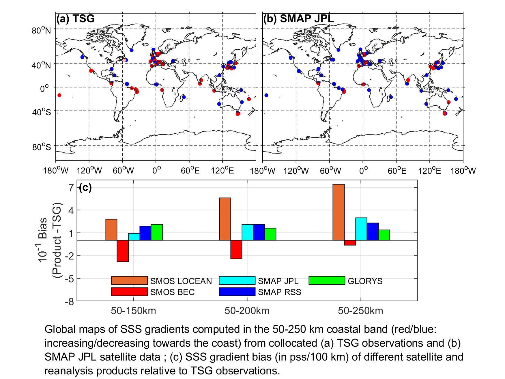
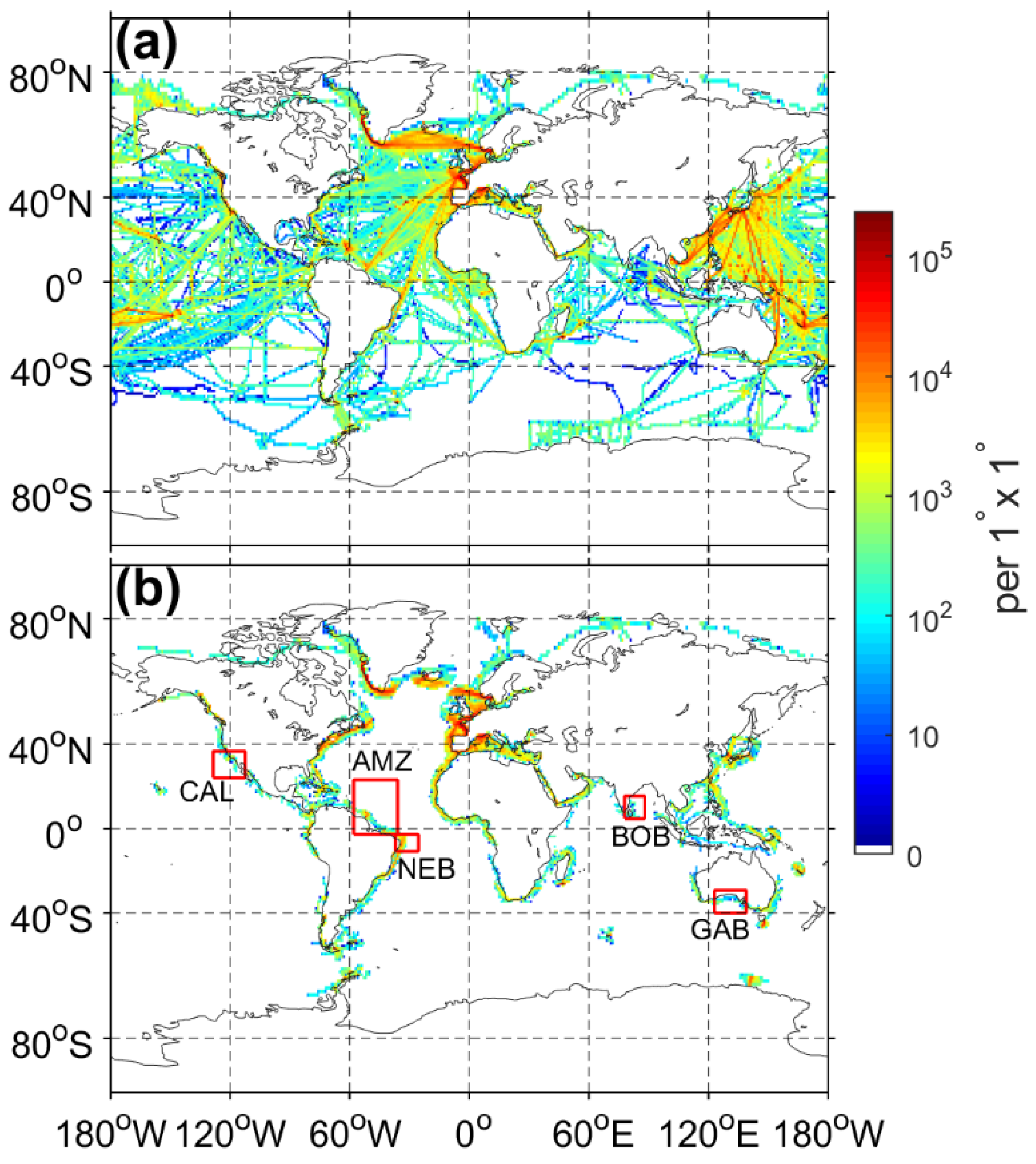
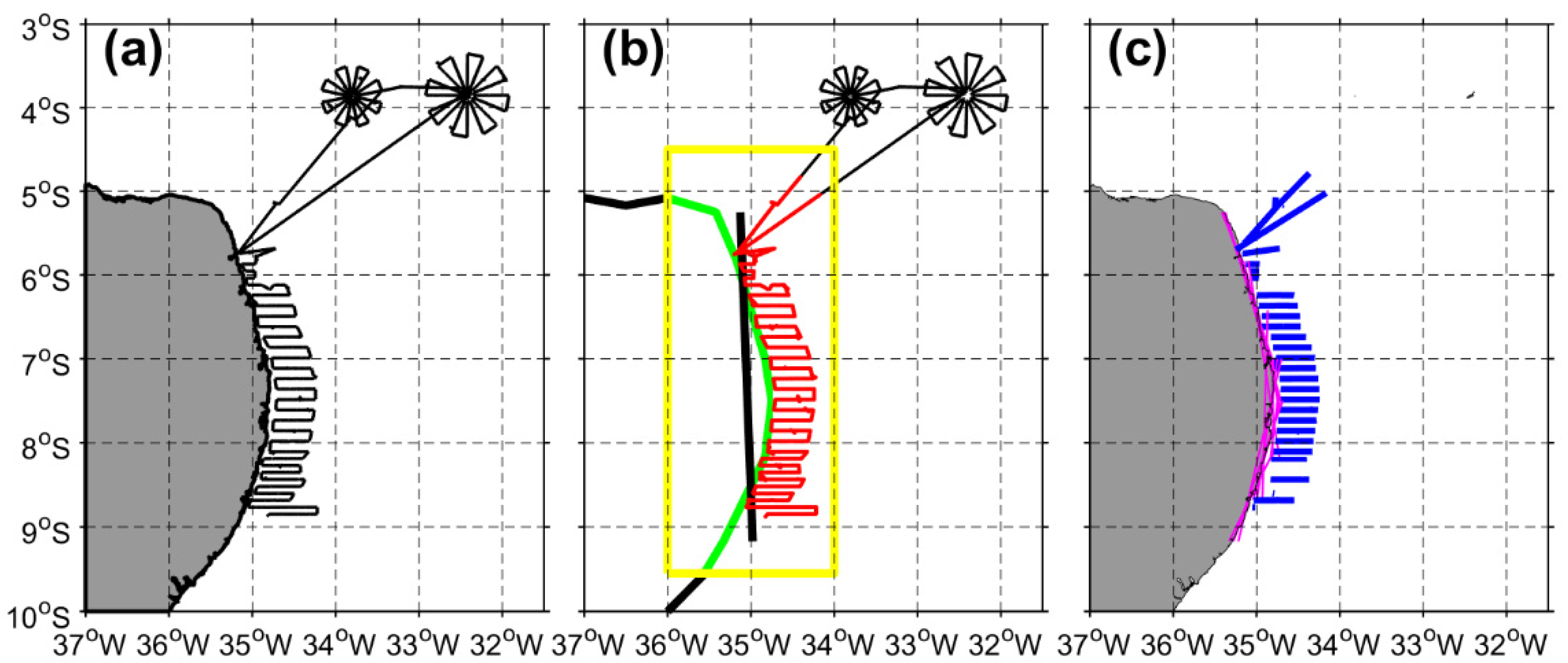
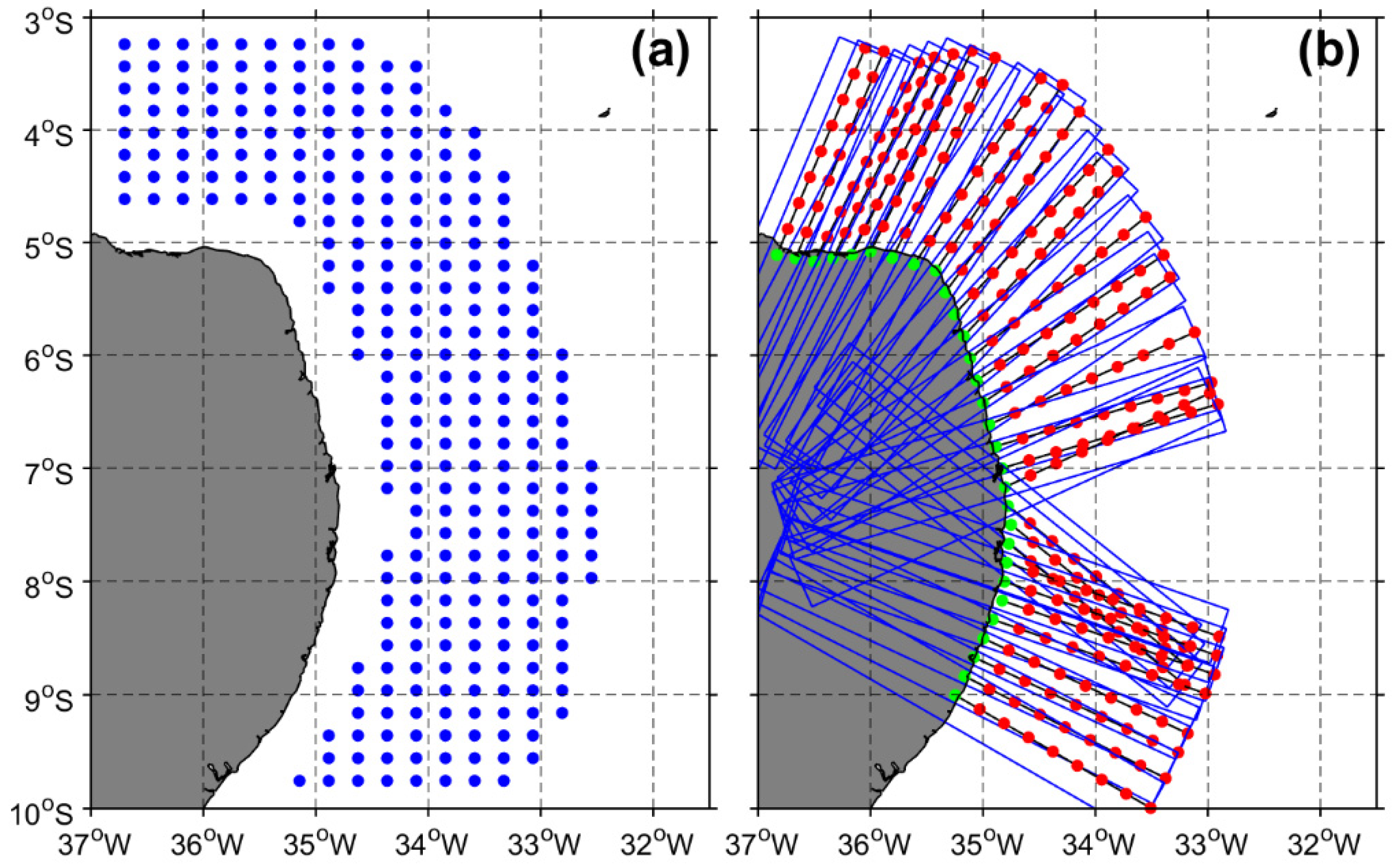
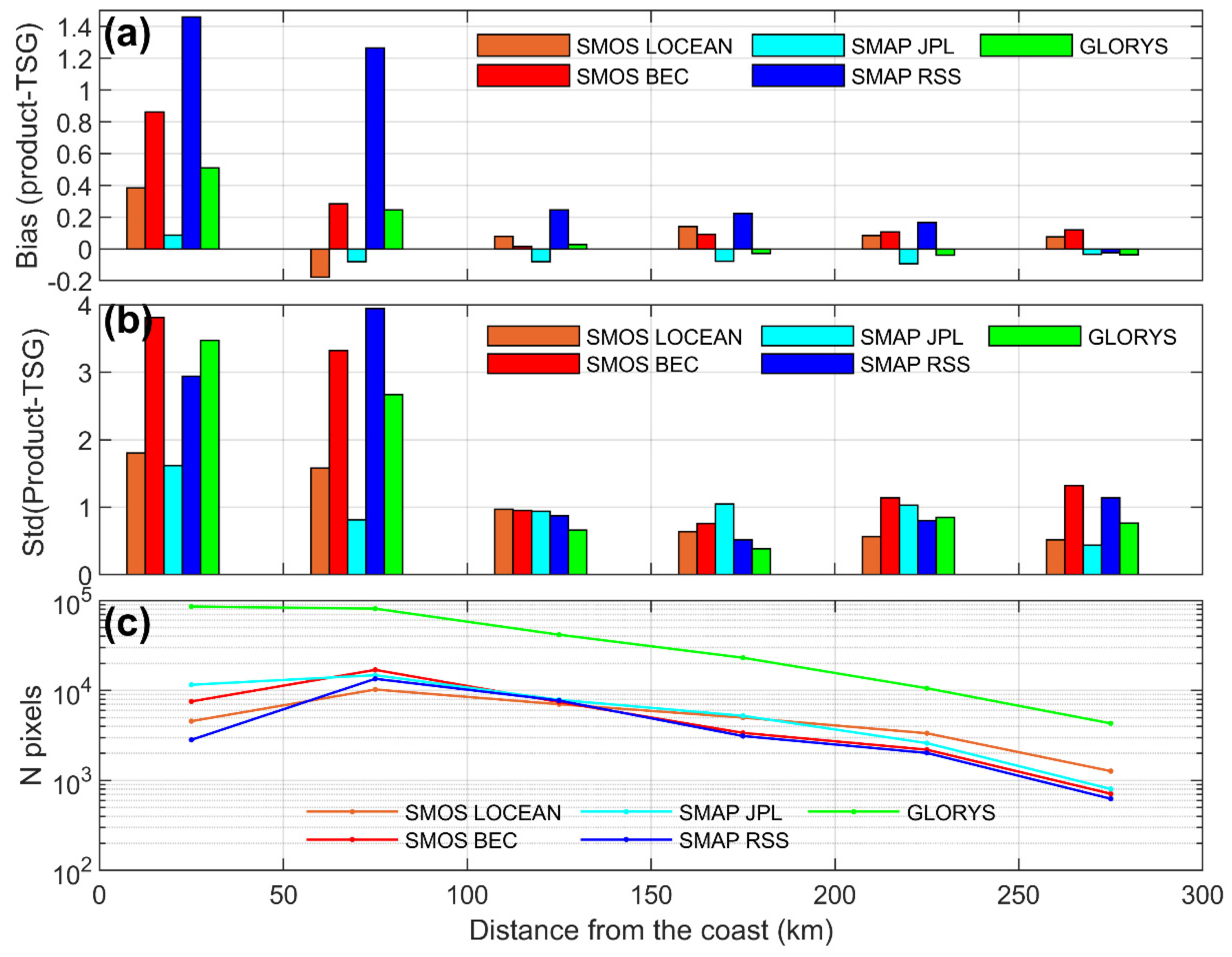
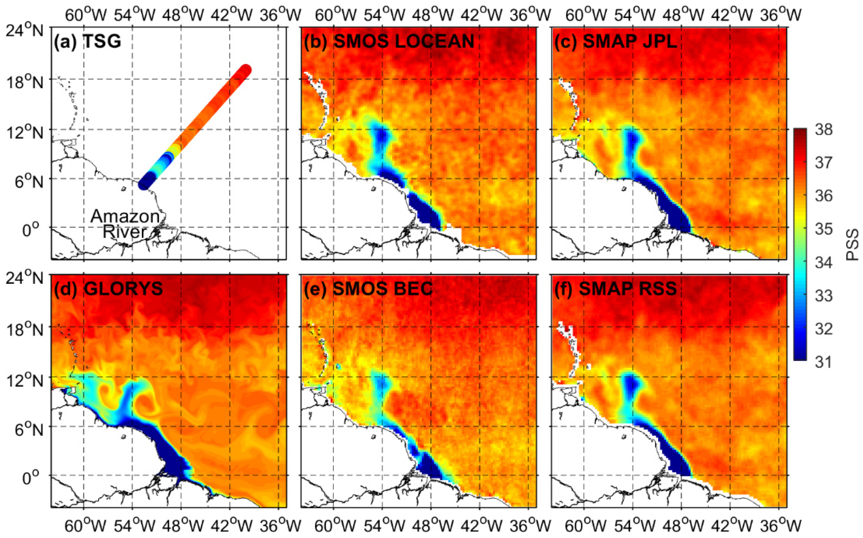
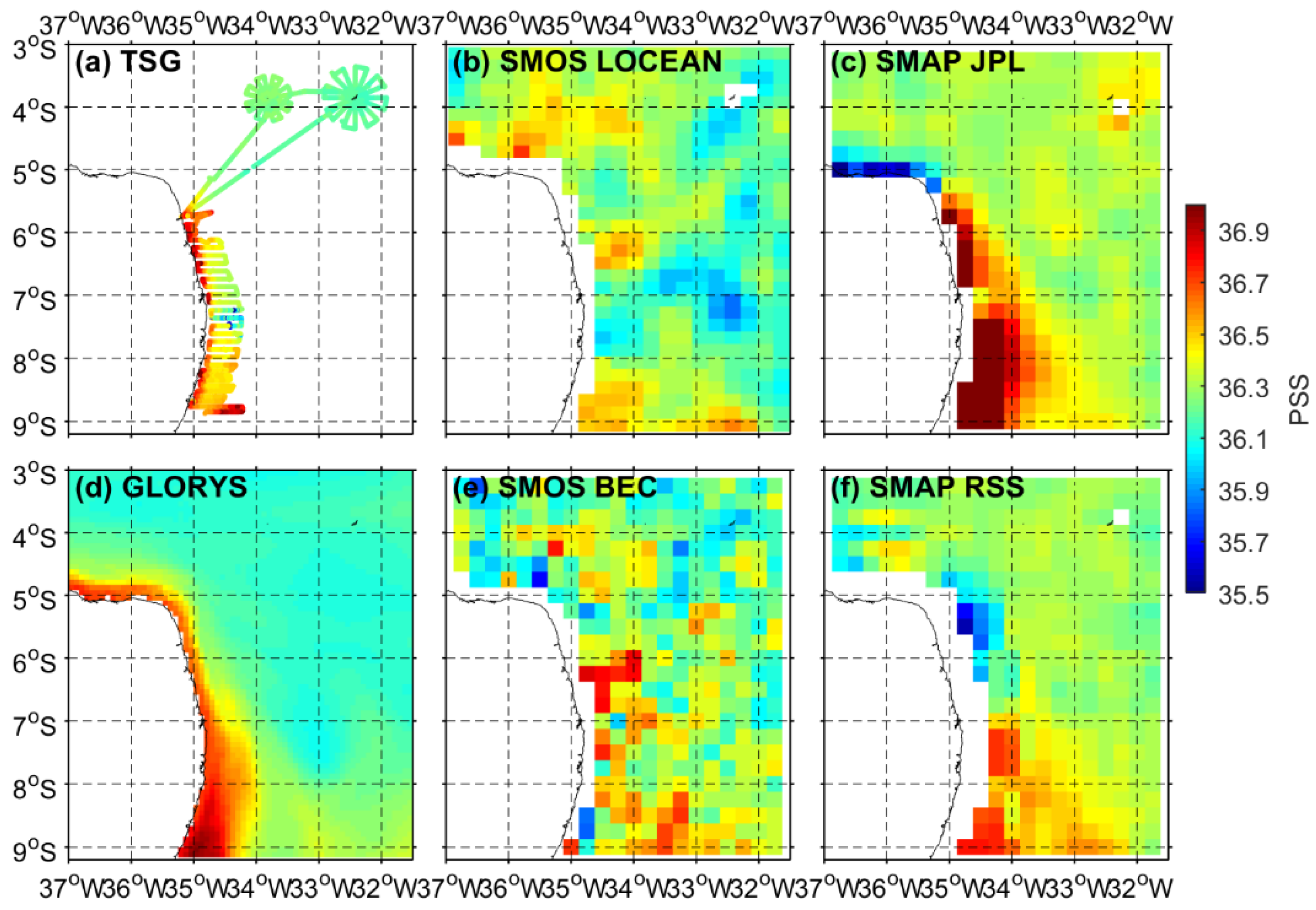
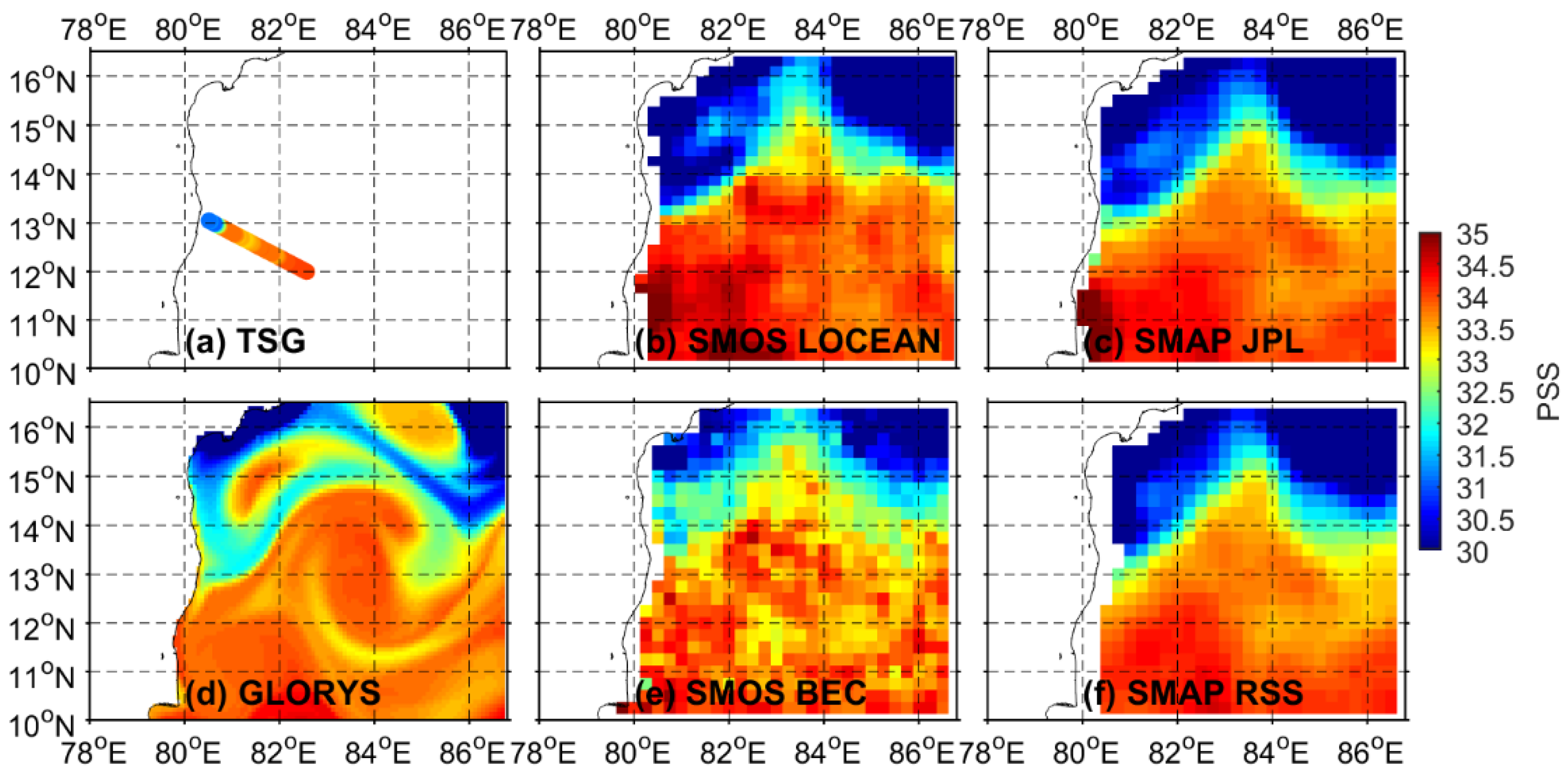
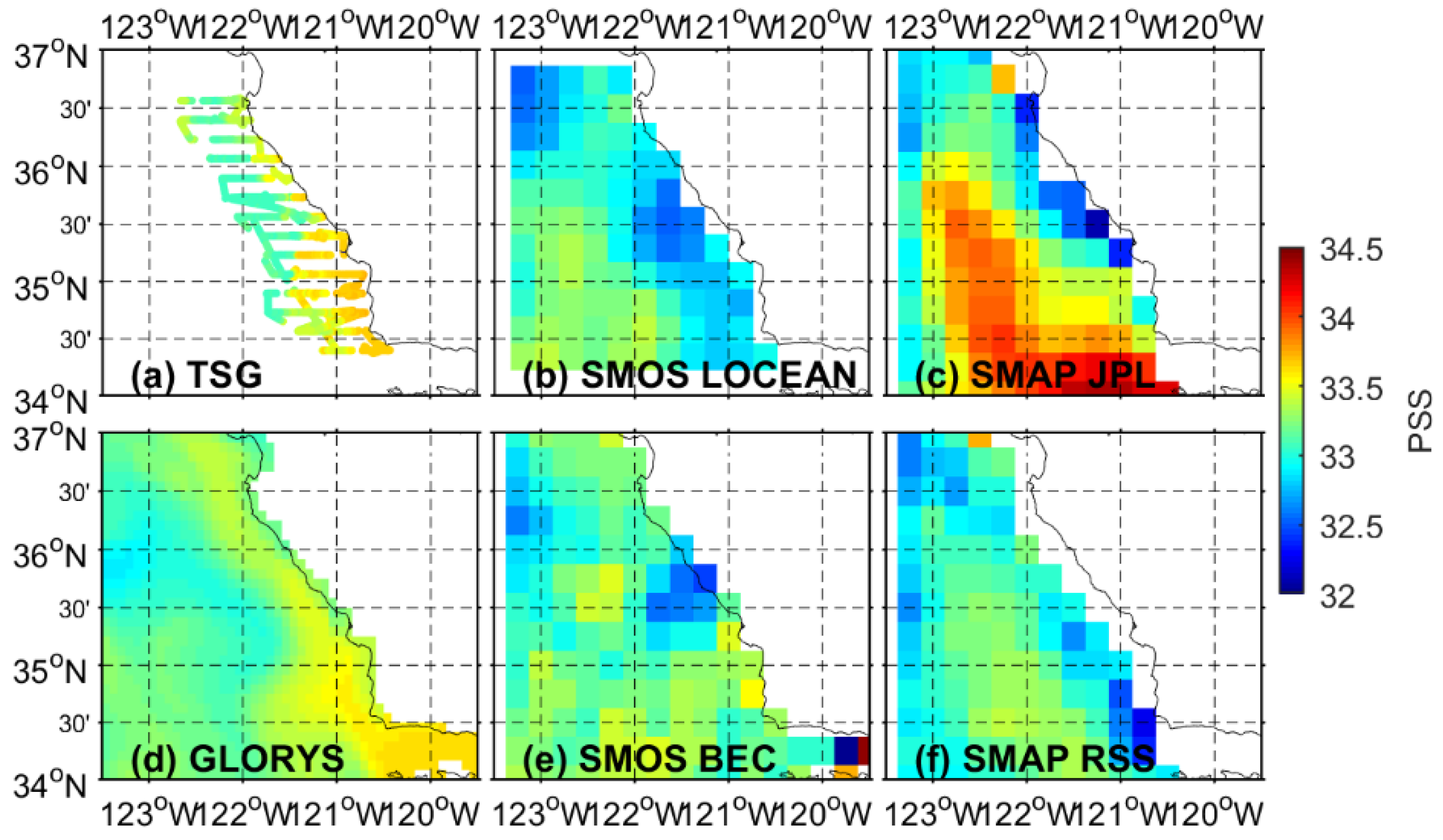
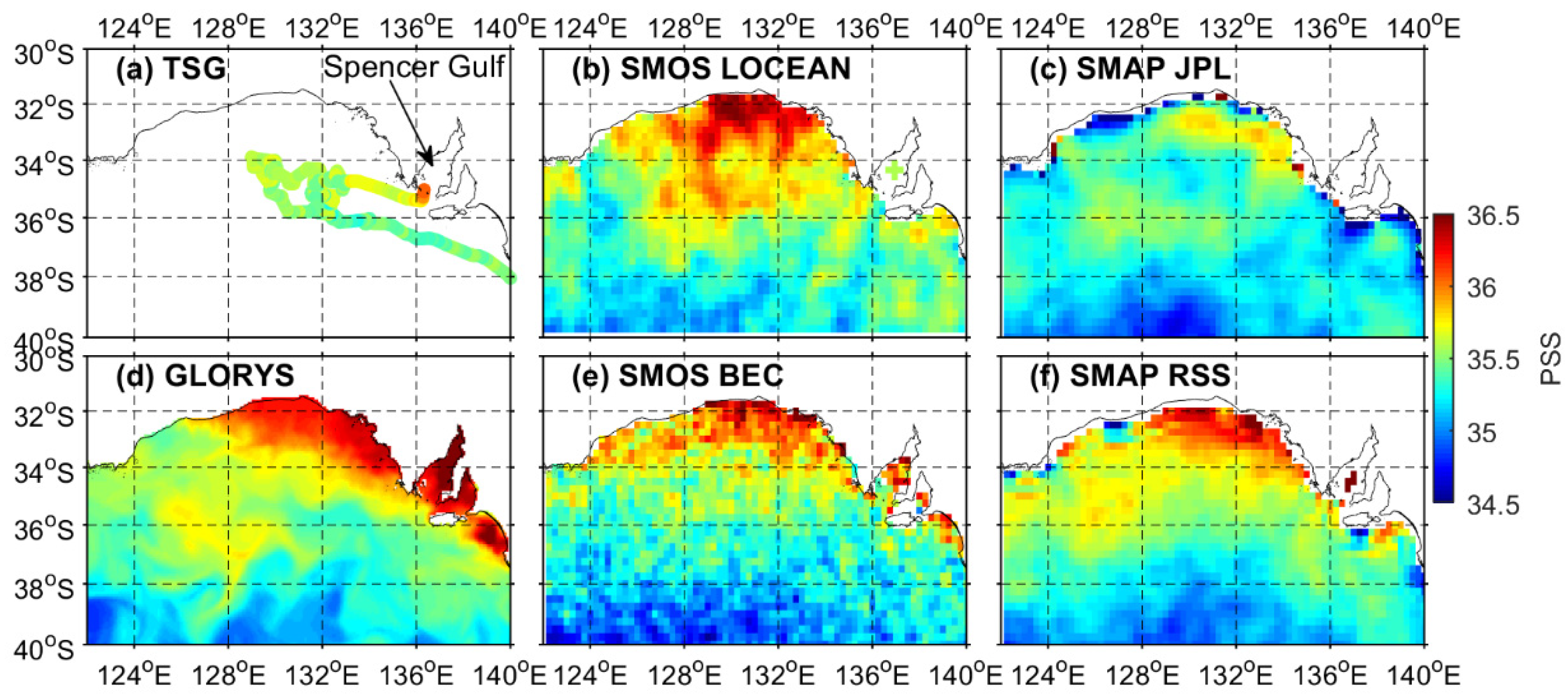
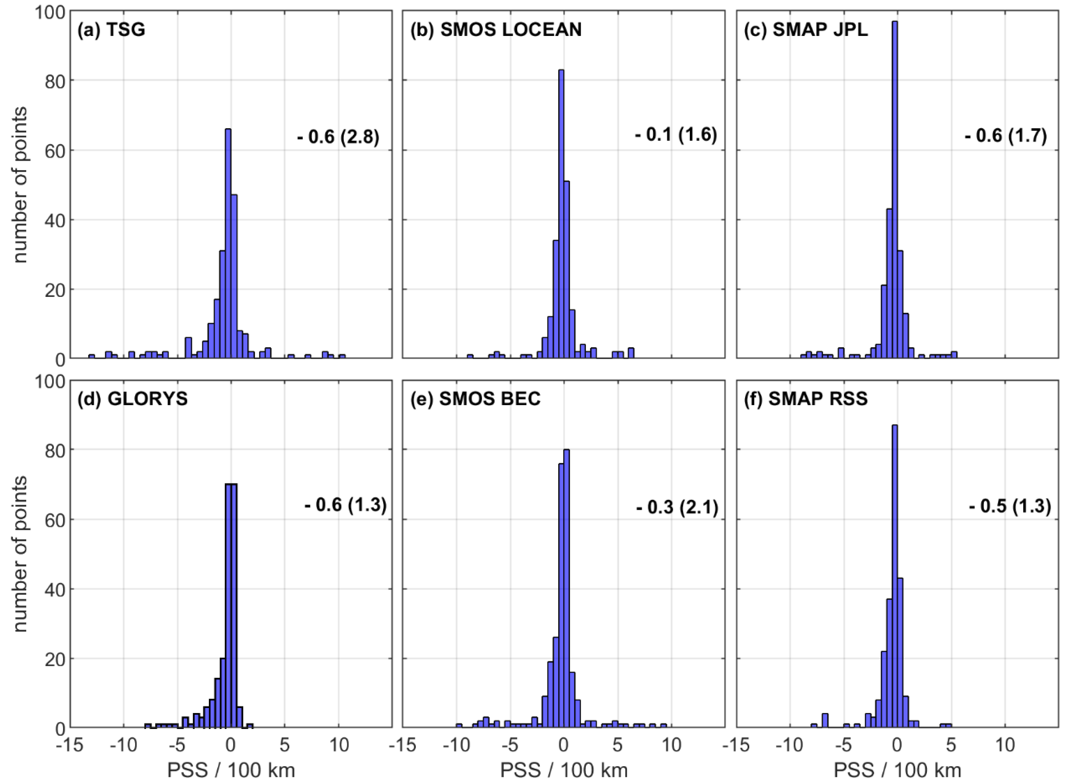
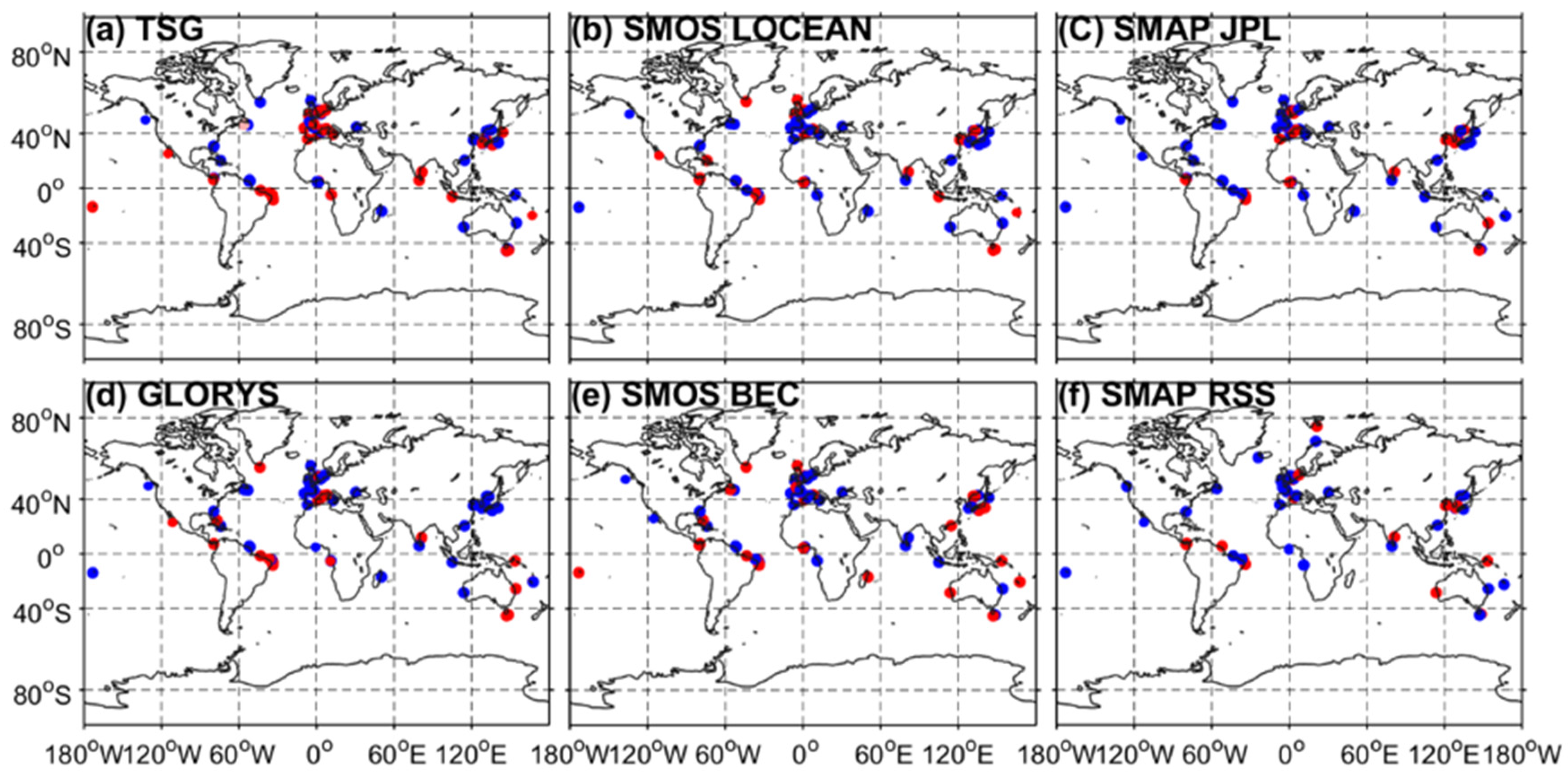
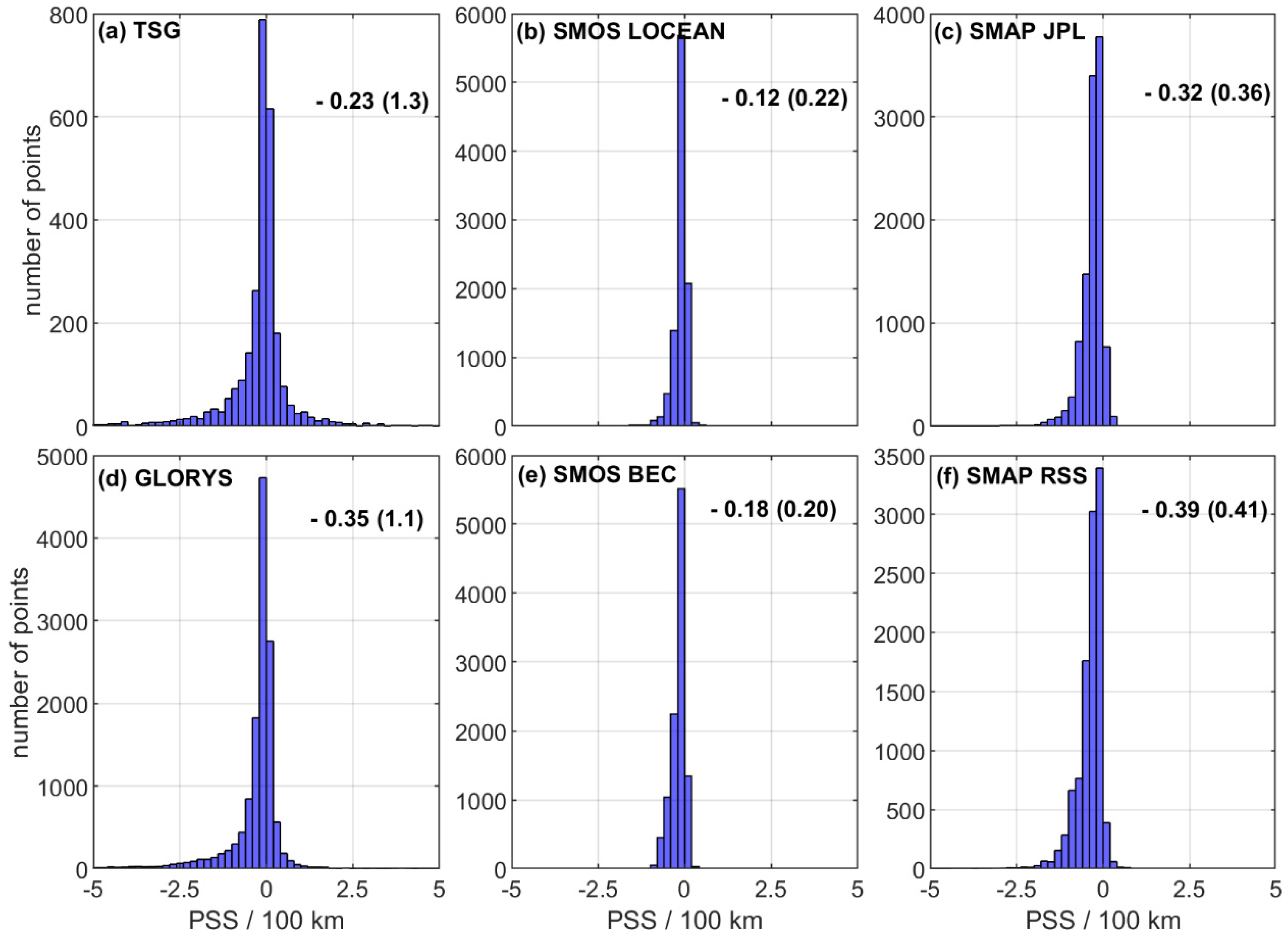
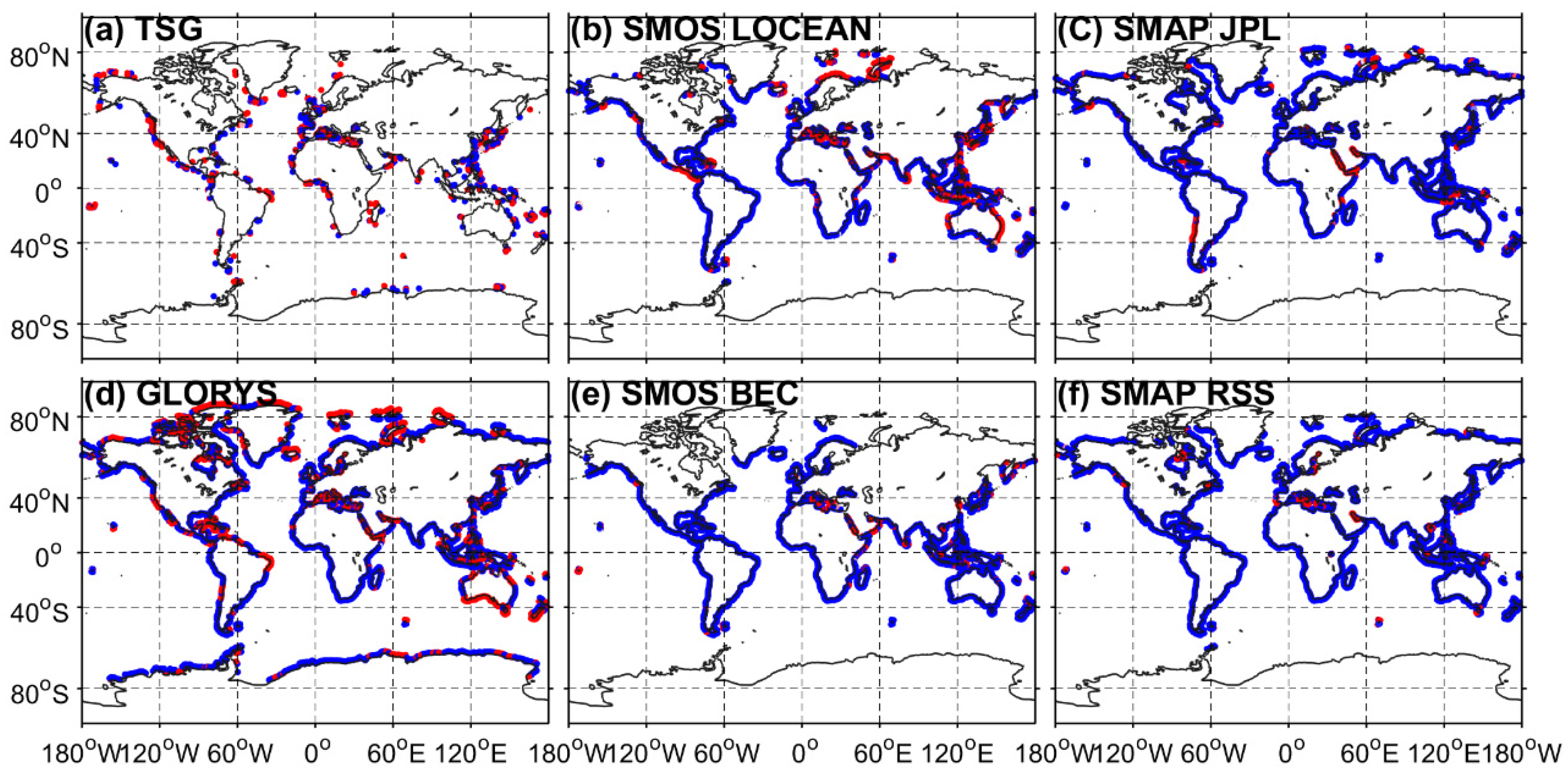
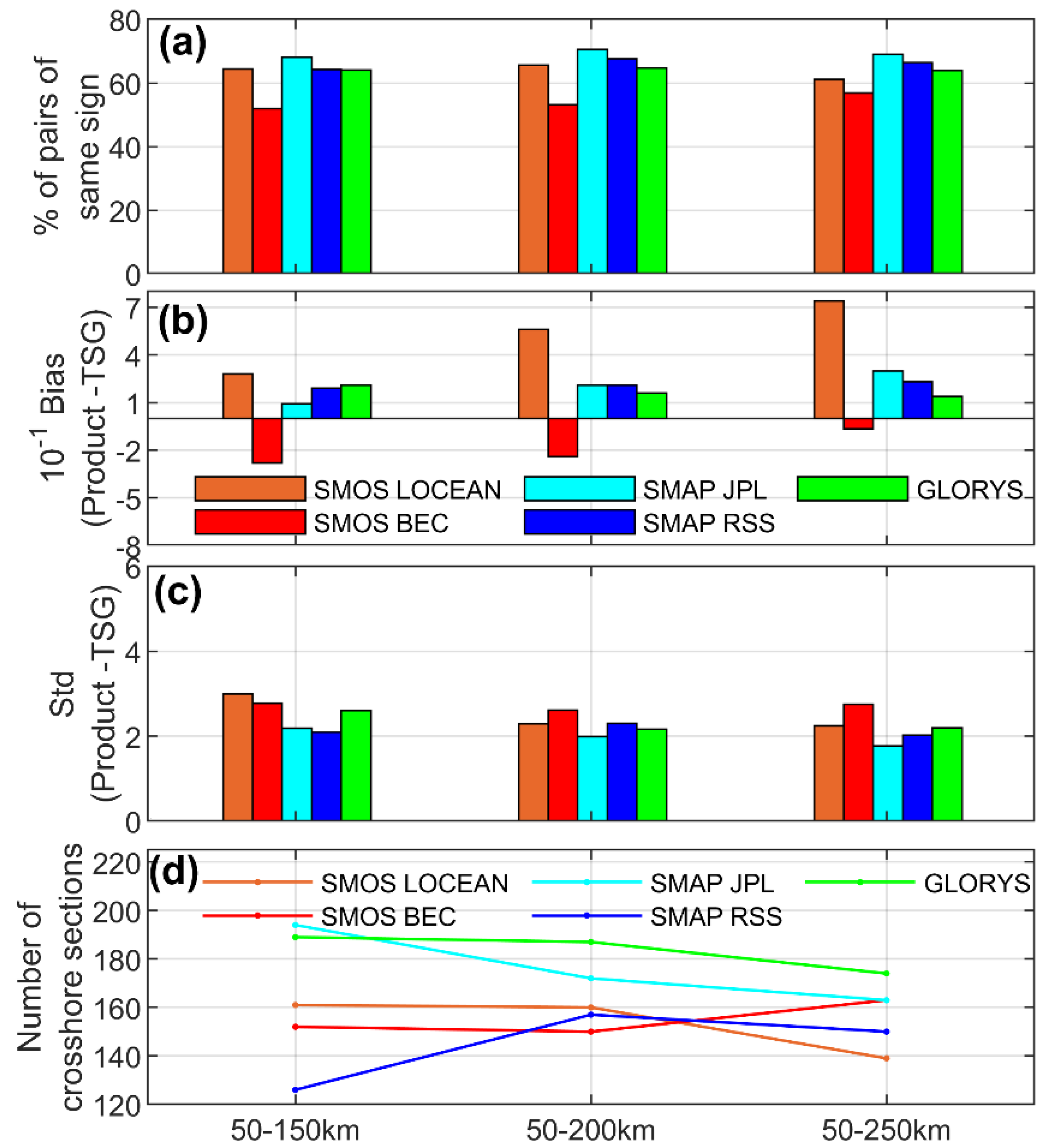
Table 1.
Regions of interest (red boxes in Figure 1a).
Table 1.
Regions of interest (red boxes in Figure 1a).
| Regions Name | Amazon River Plume (AMZ) | Northeast Brazil (NEB) | Bay of Bengal (BOB) | California Upwelling System (CAL) | Great Australian Bight (GAB) |
|---|---|---|---|---|---|
| Regions’ location | 64–35°W; 4–24°N | 37–31.5°W; 9.2–3°S | 78–86.5°E; 10–16.5°N | 123.5–119.5°W; 25–37°N | 140–122°E; 40–30°S |
| Data period | 6–9 March 2017 | 28 September–21 October 2015 | 23–24 October 2015 | 17–25 June 2019 | 28 Oct–27 Nov 2015 |
| Ship name | Toucan | RV Antea | Onyx | RV Bell Shimada | RV Investigator |
Publisher’s Note: MDPI stays neutral with regard to jurisdictional claims in published maps and institutional affiliations. |
© 2021 by the authors. Licensee MDPI, Basel, Switzerland. This article is an open access article distributed under the terms and conditions of the Creative Commons Attribution (CC BY) license (https://creativecommons.org/licenses/by/4.0/).
Share and Cite
MDPI and ACS Style
Dossa, A.N.; Alory, G.; da Silva, A.C.; Dahunsi, A.M.; Bertrand, A. Global Analysis of Coastal Gradients of Sea Surface Salinity. Remote Sens. 2021, 13, 2507. https://doi.org/10.3390/rs13132507
AMA Style
Dossa AN, Alory G, da Silva AC, Dahunsi AM, Bertrand A. Global Analysis of Coastal Gradients of Sea Surface Salinity. Remote Sensing. 2021; 13(13):2507. https://doi.org/10.3390/rs13132507
Chicago/Turabian StyleDossa, Alina N., Gaël Alory, Alex Costa da Silva, Adeola M. Dahunsi, and Arnaud Bertrand. 2021. "Global Analysis of Coastal Gradients of Sea Surface Salinity" Remote Sensing 13, no. 13: 2507. https://doi.org/10.3390/rs13132507
Note that from the first issue of 2016, this journal uses article numbers instead of page numbers. See further details here.