Oil Spill Detection in Quad-Polarimetric SAR Images Using an Advanced Convolutional Neural Network Based on SuperPixel Model


1
State Key Laboratory of Precision Measuring Technology and Instruments, Tianjin University, Tianjin 300072, China
2
Binhai International Advanced Structural Integrity Research Centre, Tianjin 300072, China
3
Faculty of Information Technology, Beijing University of Technology, No. 100 PingLeYuan, Chaoyang District, Beijing 100124, China
4
Institute of Photogrammetry and Remote Sensing, Chinese Academy of Surveying and Mapping, Beijing 100036, China
*
Author to whom correspondence should be addressed.
Remote Sens. 2020, 12(6), 944; https://doi.org/10.3390/rs12060944
Submission received: 9 February 2020
/
Revised: 10 March 2020
/
Accepted: 12 March 2020
/
Published: 14 March 2020
(This article belongs to the Special Issue Remote Sensing of the Oceans: Blue Economy and Marine Pollution)
Abstract
:Oil spill detection plays an important role in marine environment protection. Quad-polarimetric Synthetic Aperture Radar (SAR) has been proved to have great potential for this task, and different SAR polarimetric features have the advantages to recognize oil spill areas from other look-alikes. In this paper we proposed an oil spill detection method based on convolutional neural network (CNN) and Simple Linear Iterative Clustering (SLIC) superpixel. Experiments were conducted on three Single Look Complex (SLC) quad-polarimetric SAR images obtained by Radarsat-2 and Spaceborne Imaging Radar-C/X-Band Synthetic Aperture Radar (SIR-C/X-SAR). Several groups of polarized parameters, including H/A/Alpha decomposition, Single-Bounce Eigenvalue Relative Difference (SERD), correlation coefficients, conformity coefficients, Freeman 3-component decomposition, Yamaguchi 4-component decomposition were extracted as feature sets. Among all considered polarimetric features, Yamaguchi parameters achieved the highest performance with total Mean Intersection over Union (MIoU) of 90.5%. It is proved that the SLIC superpixel method significantly improved the oil spill classification accuracy on all the polarimetric feature sets. The classification accuracy of all kinds of targets types were improved, and the largest increase on mean MIoU of all features sets was on emulsions by 21.9%.

1. Introduction
Marine environment plays a crucial part in global ecosystems. Oil spill is one of the main marine pollution, which will cause serious damage to ocean ecology and resources. In 2010, the accident of the Gulf of Mexico oil spill lasted for about three months. Beaches and wetlands in many states of the United States were destroyed and local marine organism was devastated [1]. Thus it is necessary to monitor sea surface and detect oil spill. Remote sensing plays a crucial role in achieving this goal, and relevant methods have been effectively applied to oil spill detection.
Space-borne Synthetic Aperture Radar (SAR) is widely applied for oil spill detection due to its all-weather and all-time ability and wide area coverage. Full polarization SAR data provides four channels according to the transmit and receive mode of radar signal and they are HH, HV, VH and VV channels. The clean sea can be regarded as a rough surface, while the smooth oil spill layer usually floats on the water surface, existing as dark spots since it dampens capillary waves, short gravity waves and Bragg scattering [2]. The general steps for oil spill detection are divided into: (1) spot extraction, (2) feature extraction, (3) classification [3]. Early researches mainly focused on textual information of dark spots area. Several textual features including first invariant planar moment and power-to-mean ratio were extracted from SAR data, supplemented by statistical model or machine learning, to perform oil spill detection [4,5]. Some experiments were carried out to perform oil spill detection on different band SAR images [6,7]. Yongcun Cheng et al. used VV channel data acquired by COSMO-SkyMed to monitor oil spill and simulate a model [8]. M. Migliaccio et al. proposed a multi-frequency polarimetric SAR processing chain to detect oil spill in the Gulf of Mexico, and has been applied successfully [1]. These methods could successfully distinguish oil spill area from sea surface, and they are known as mature classification algorithms.
However, several environmental factors including low-speed winds, internal wave and biogenic films also appear as dark spots in SAR images [9], and they are called look-alikes. The most challenging thing of oil spill detection from SAR images is to distinguish the oil spill area from these look-alikes. That is the main obstacle of the early researches of texture analysis focused on single pol-SAR data. Oil spill area may experience complex deformation on the sea surface, which is easy to be confused with look-alikes. Moreover, a large amount of data are required for texture analysis. These problems become major hindrances for high-accuracy oil spill detection. With the new development of SAR satellites in recent years, the research focus of oil spill detection began to incline to dual-pol or quad-pol SAR image, and the derived compact SAR [10], which not only retain texture characteristics of dark spots area, but also provide a lot of polarized information. Polarimetric decomposition essentially reflects the scattering modes of microwave on the sea surface, which highlights the subtle differences of different ocean objects [11]. Many polarized parameters extracted from different SAR channels has been proved to have great ability to perform high accuracy oil spill detection [12,13,14,15]. On the perspective of polarized feature, S. Skrunes used k-means classification method to detect oil spill area on several polarized parameters [16]. With the rise of machine learning algorithms in recent years, neural networks have also been applied into oil spill detection. Yu Li et al. performed several comparative experiments between different machine learning classifiers based on multi polarized parameters [17], and the differences between fully and compact polarimetric SAR images [18] were explored.
Meanwhile, as a classical feedforward neural network, convolutional neural network (CNN) is widely used in image classification and recognition. Since it was proposed in 1989, CNN has experienced many improvements and changes, and derived several classic network structures such as Inception, Resnet and Cliquenet [19,20,21]. Min Lin et al. used the global average pooling (GAP) layer to replace the fully connection layer to reduce the parameter amount in 2014 [22]; Andrew Howard et al. put forward the depthwise separable convolution in MobileNet [23,24], which can maintain high accuracy even when the amount of parameters and calculation is reduced.
In 2015, Jonathan Long et al. proposed a fully convolutional network (FCN) with transposed convolution for image semantic segmentation [25]. The end-to-end operation is implemented with an encoder-decoder structure, and the classification prediction is given for each pixel on the image. The concept of dilated convolution into semantic segmentation in 2016, and it greatly improved classification accuracy [26]. Follow by that, advanced models have been developed for high precision segmentation, and they are Unet, Linknet and Deeplab series [27,28]. The encoder-decoder structure of semantic segmentation model based on CNN has been used in oil spill detection in recent studies [29,30], and achieved high accuracy. With the application of TerraSAR-X and other SAR satellites, dual-polarized SAR images are also introduced into oil spill detection. Daeseong Kim et al. extracted polarized parameters from dual-pol TerraSAR-X images, successfully mapped oil spill area with artificial neural networks [31].
The concept of superpixel is an image segmentation technology proposed in 2003 [32]. It refers to an irregular pixel block with certain visual significance. It is composed of adjacent pixels with similar texture, color brightness and other characteristics. The similarity of features between pixels are used to form a group of pixels, and image are expressed by a small number of superpixels. Superpixel greatly reduces the complexity of image post-processing, and it is used as a pre-processing step for image segmentation algorithm. Simple Linear Iterative Clustering (SLIC) is a widely used superpixel segmentation method [33], and has been introduced into some SAR scenes. Some researchers also use multi-chromatic analysis to perform target detection and analysis on SAR images [34,35].
Many current oil spill detection methods only divided images into oil or non-oil areas, which may cause false alarm and cannot recognize every target on the sea surface. The classification method combining neural networks also could not distinguish oil spill and look-alikes well, while the flexible structure of CNN provides the possibility to solve these problems. It allows a variety of parameters input, can simultaneously take into account the task of dark spots extraction and classification and identify every target on the sea surface. In this paper we proposed an oil spill detection method using SLIC superpixel and semantic segmentation algorithm based on CNN, combining several convolution kernels including dilated and depthwise separable convolution. It allows multiple-parameters input and realize pixel-level oil spill area classification, which finally realize further accuracy improvement. We carried out experiments on five groups of polarized parameters extracted from SLC quad-polarimetric SAR data of Radarsat2 and Spaceborne Imaging Radar-C/X-Band Synthetic Aperture Radar(SIR-C/X-SAR), and evaluated the classification results of superpixel segmentation combined with polarized parameters. The experiments results show that our method could effectively extract and classify dark spots on a SAR image. SLIC superpixel could further improve classification accuracy of oil spill area, and Yamaguchi 4-component decomposition combined with SLIC superpixel classification is considered the most suitable parameters for oil spill detection in our case.
2. Materials and Methods
2.1. Overall Framework
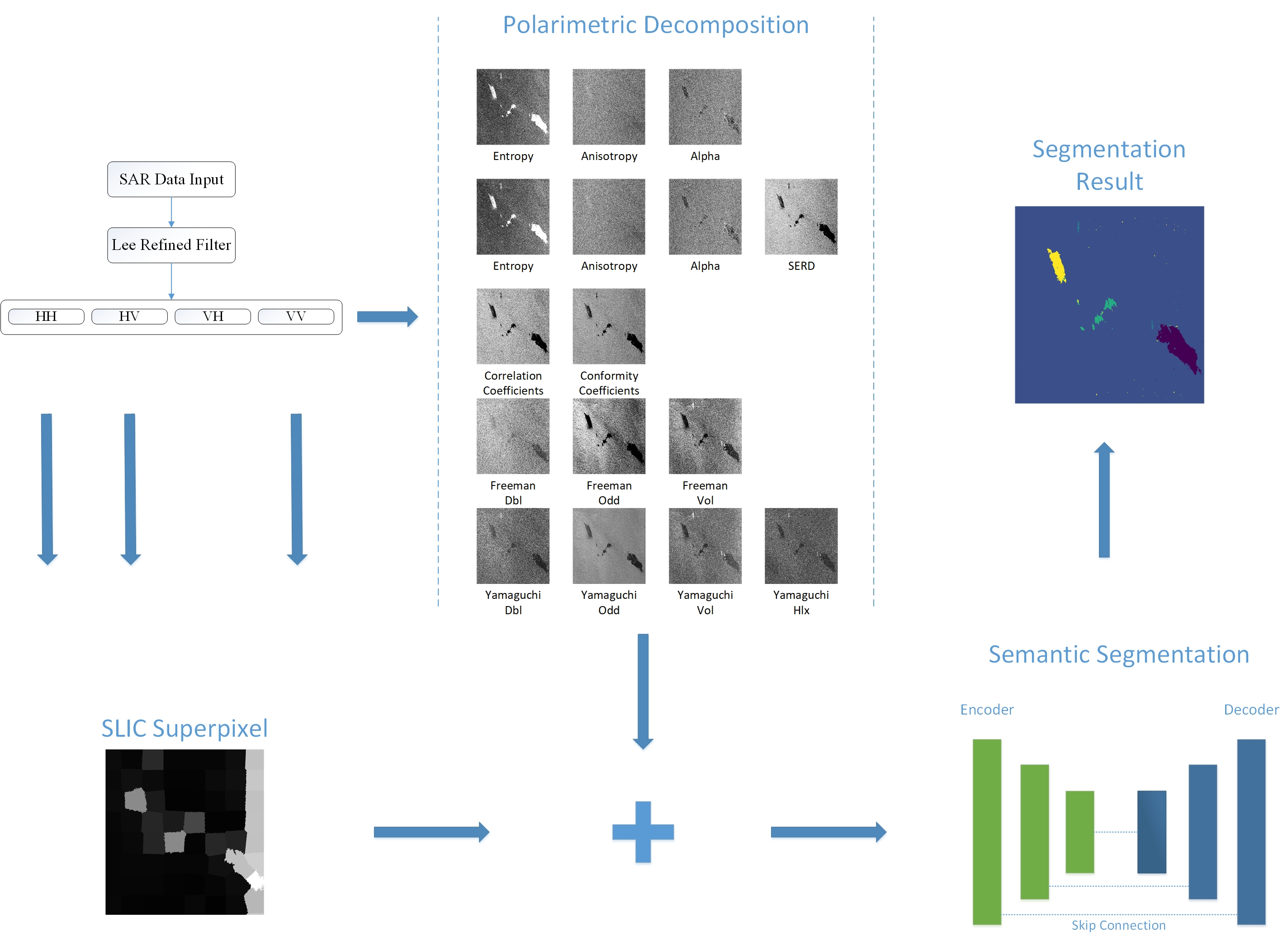
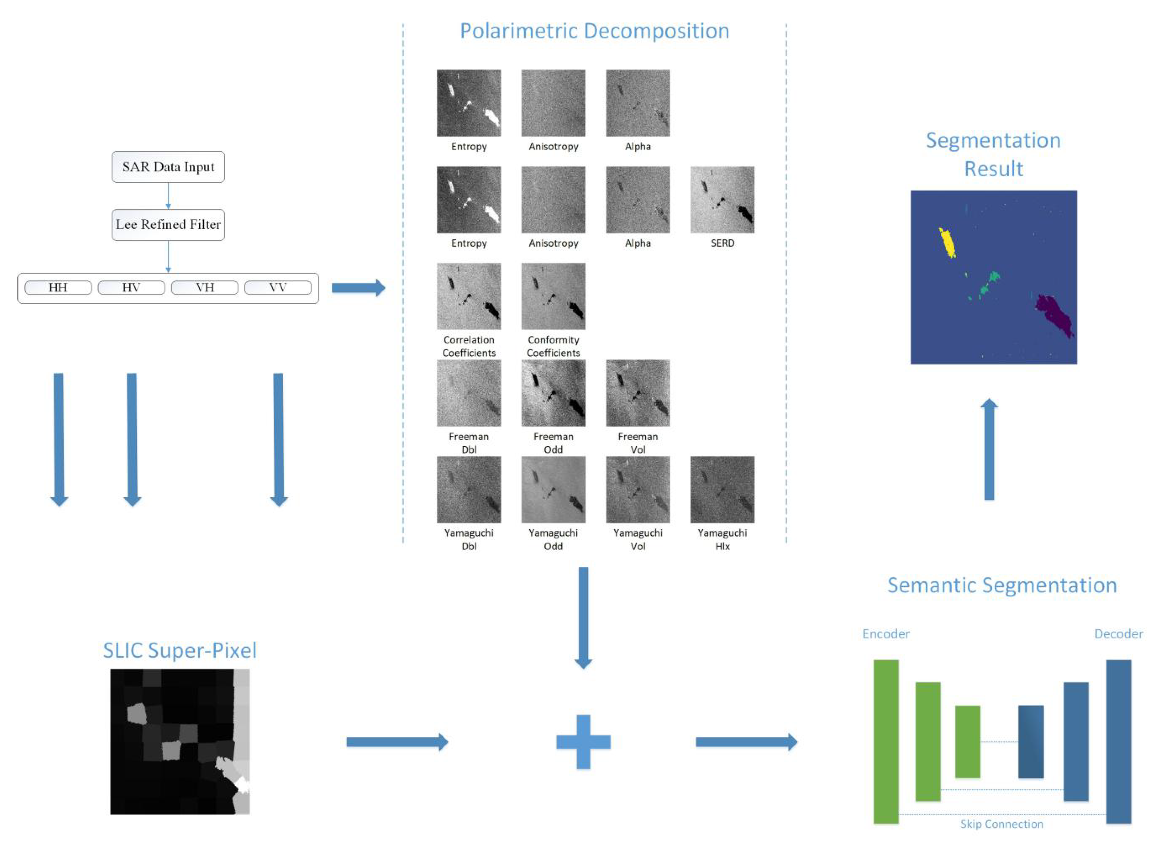
The flowchart of our oil spill detection method is illustrated as Figure 1. The four channels data was processed by Lee refined filter firstly, and different polarized parameters were then extracted from these four channels. All polarized parameters used in our experiments are divided into five groups according to different scattering principles and calculation methods. For monostatic SAR system, reciprocity always holds, which means that the complex scattering coefficient obeys HV = VH. For this reason, HV is considered for cross polarization channel in the analysis. Three channel data should be used to generate image in CIElab color space for SLIC superpixel model. We choose data of HH, HV and VV channel to do it, since co-polarized channels (HH/VV) data contains more polarized information than cross-polarized channels (VH/HV) [36]. The HH, HV and VV data were also used to calculate SLIC superpixels. Section 2.2 and Section 2.3 explains the method used to extract polarized parameters and they are both set as the input of neural network models. The neural network is composed of an encoder and a decoder section. The output of the neural network is segmentation results of oil spill detection.
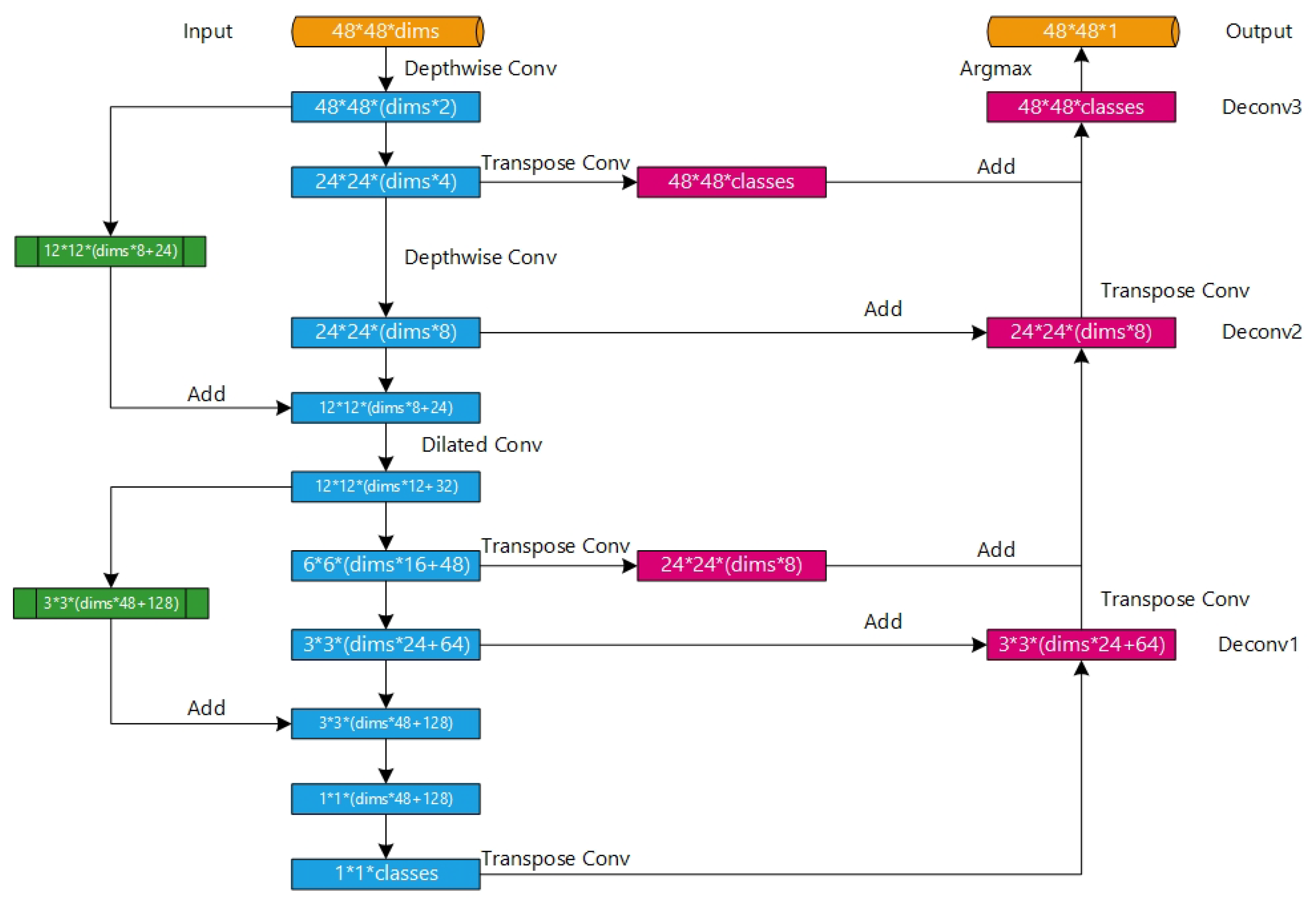
We designed a semantic segmentation model based on CNN as the classifier, as shown in Figure 2. The dims in the diagram represents the number of polarization parameters, since multiple polarization modes are applied in our work, the network parameters will be adjusted according to the parameter of dims. The depthwise separable convolution and dilated convolution was used in several layers in the bottom parts. The subsequent encode task is completed by standard convolution layer. Green blocks represent a skip connection structure similar to residual learning [19], in order to make top layers accessible to the information from bottom layers and help train the network easier. The feature maps extracted by encoder is decoded by progressive transposed convolution layers, and skip connection is also applied to absorb more features. The specific principle and implementation of network are explained in Section 2.4 in detail.
The different polarized parameters groups and superpixel segmentation results will be combined to input into the neural networks for training. The output is the result of oil spill detection. Finally, Mean Intersection over Union (MIoU) was calculated between segmentation result and annotation images to evaluate the accuracy.
2.2. Polarimetric Decomposition
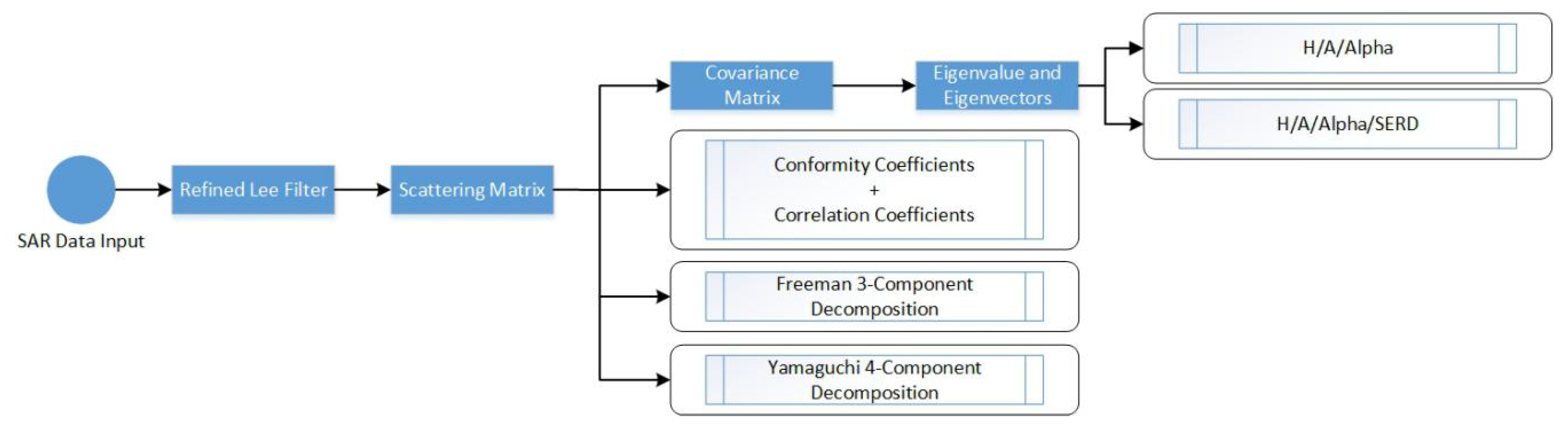
The whole process of extracting polarimetric parameters is shown in Figure 3. The boxes are different polarized parameter combinations for classification. This section will explain the calculation method of different polarized parameters in the followings.
2.2.1. H/A/Alpha Decomposition
The scattering matrix of a fully polarimetric SAR image can be expressed as
where and represent the amplitudes and phases of the complex scattering coefficients, each complex element donates a polarization component. The two crossed-polarized terms are identical in Radarsat-2, i.e., .
Polarization covariance matrix C and coherency matrix T contain abundant physical information of polarization characteristics of ocean objects. Cloude and Pottier outlined a scheme for parameterizing polarimetric scattering problems based on matrix T in 1997, the covariance matrix can be derived by
where represents conjugate, 〈 〉 stands for multilook with an average window (we set the window size to 3, the same is true in later equations). The expression of matrix T is listed as follow:
can be transformed into according to formula , , it can also be expressed in another form
where H donates transpose conjugate, and the formula of is
The column vectors , and of are the eigenvectors of matrix , corresponding to eigenvectors , and . Cloude decomposition regards the scattering behaviors of targets as the superposition of three independent scattering behaviors, and the probability of three eigenvectors, which represents the weights of each basic scattering can be calculated by
The polarimetric entropy describes the randomness of the scattering mechanisms and is defined by
The formula of anisotropy is
and the mean scattering angle is
where , donates the eigenvalue of .
2.2.2. Single-Bounce Eigenvalue Relative Difference
Allain et al. proposed Single-Bounce Eigenvalue Relative Difference (SERD) based on Cloude decomposition in 2004. The correlation between co-polarized and cross-polarized channels is almost equal to 0 for sea surface microwave scattering, so the matrix can be simplified as
and the eigenvalue of matrix can be calculated by
The first two eigenvalues are related to the co-polarized backscatter coefficient, and the third one is related to the cross-polarized channel and multiple scattering. Calculate the value of scattering angle according to the eigenvectors corresponding to eigenvalues and to distinguish the type of scattering mechanisms: the eigenvalue corresponds to a single scattering when , and it is a double scattering when . The SERD is defined as
when or , and when or .
SERD is very sensitive to the surface roughness. A large value of SERD indicates a strong single scattering in the scattering process of the target, while the small SERD value indicates weak single scattering. For the high entropy scattering area of oil spill surface, the scattering is composed of many kinds of scattering mechanisms. Single scattering is not dominant, that is, the SERD value at oil film is relatively small, and then it can be used for oil spill detection.
2.2.3. Co- and Cross- Polarized Decomposition
This section will introduce two parameters based on the scattering matrix: co-polarized correlation coefficients and conformity coefficients. Correlation coefficients can be expressed as
The conformity coefficients were firstly introduced into compact polarimetric SAR to estimate soil moisture by Freeman et al. [18]. Extending the conformity coefficients to quad-polarimetric SAR, it can be expressed as
2.2.4. Freeman 3-Component Decomposition
Freeman and Durden [11] proposed a three-component scattering model for polarimetric SAR data in 1998, and it includes three simple scattering mechanisms: volume (or canopy) scattering, double-bounce scattering and rough surface scattering. Assuming those three scatter components are uncorrelated, the scattering process of radar wave on the sea surface can be regarded as the composition of these three mechanisms, so the model for total backscatter is
where , and are the contribution of surface, double-bounce and volume scattering to the VV cross section. Once , and are estimated, we can also get contributions of three scatter to HH, HV and VH channels. in the formula is defined by
and donate the reflection coefficients of vertical surface for H and V polarizations, while and are the Fresnel reflection coefficients of horizontal surface. The propagation factors and are used to make the model more general, represents any attenuation and phase change of the V and H polarized waves when they propagate from the radar to the ground and back again. α = −1 when is positive, if is negative, .
The volume scattering contribution can be calculated directly from Equation (15d). We can estimate the contribution of each scattering mechanism to the span P
with
Then we can use Equations (15)–(18) to calculate the scattering power of three mechanisms: , and . They are the result of Freeman decomposition.
2.2.5. Yamaguchi 4-Component Decomposition
In 2005, Yamaguchi et al. [12] proposed a four component decomposition method based on Freeman decomposition, included the helix scattering power as the fourth term for a more general model, which is essentially caused by the scattering matrix of helices and is mainly used in urban areas. What is more, Yamaguchi decomposition modify the volume scattering matrix according to the relative backscattering magnitudes of versus .
Assume the magnitude of the helix scattering power , the corresponding magnitude of becomes , and the power relation becomes
and we can get the following five equations , , , , , by comparing the covariance matrix element:
can be measured directly. The volume scattering coefficient is calculated by
and is calculated as the same way as Freeman decomposition, so we can get contribution of four mechanisms: , , and . The scattering powers , , and corresponding to surface, double bounce, volume and helix scattering contributions can be obtained by
, , and are the results of Yamaguchi decomposition.
2.3. SLIC Superpixel
The superpixel algorithm was first proposed in 2003 by Xiaofeng Ren et al. [32]. Adjacent pixels with the same attribute are divided in one region (one superpixel) and then the whole image can be indicated by a certain number of superpixels, which allows better performance for subsequent image processing. SLIC adopted k-means algorithm to generate superpixels. The algorithm limited the search space to a region proportional to the size of superpixels, and reduced the number of distance calculation in optimization and the linear complexity of pixels.
The SLIC segmentation result relies only on the number of superpixels k. Each superpixel has approximately the same size. These k initial cluster centers are sampled on a regular grid with S pixel intervals. S can be calculated by , where N is the number of pixels.
Each pixel i is assigned with the nearest clustering center if their search area could overlap its position, then SLIC allows faster clustering than traditional k-means does. The distance measurement determines the closest clustering center for each pixel i. The expected spatial range of the superpixel is an area of approximate size . A similar pixel search is performed in the area around the center of the superpixel.
SLIC realizes the above steps based on labxy color image plane space. The value of the pixel is expressed as in CIELab color space. However, the position of the pixel changes with the size of the image. In order to combine them into a single measurement, we need to standardize the color proximity and spatial proximity by their maximum distances and in the cluster. Then can be calculated by
where . When is fixed as a constant m, the Equation (24c) can be listed as the following:
where in gray-scale. m allows us to balance the relative importance between and . When m increases, the superpixel result depends more on the degree of spatial proximity.
Once each pixel has been associated with the nearest cluster center, the update step adjusts the cluster center to the average vector of all pixel. norm is used to calculate the residual error E between the new and the previous cluster center position. The allocation and iterative process ends when E is less than the setting threshold. In our experiments, we transform the HH, HV and VV channel SAR data to labxy color space for superpixel calculation.
2.4. Semantic Segmentation Algorithm
We constructed a refined segmentation method based on CNN to perform oil spill detection. The structure used in our network will be described in details in the followings.
2.4.1. Convolutional Layer and Dilated Convolution
CNN has been widely used in image classification and object detection for its good generation ability. Compared with traditional neural networks, CNN imitates the human visual nerve and allows automatic feature extraction. Two main processes in the training of CNN are forward propagation and backward propagation. Forward propagation expresses the transmission of characteristic information, while backward propagation mainly uses error information to correct model parameters.
Convolutional layer is the core component of CNN. In forward propagation, it sets up a filter kernel to slide on the input tensor and obtain image features, the number of layers of these kernels equals to the input tensor. Convolution operations can be expressed as
and are weights and biases that need to be trained in neural networks, while represents the activation function, herein Rectified Linear Units(ReLU) function and function were used, and their equations are
The backward propagation process of neural networks depends on the backward derivation of the output layer (loss function) and the calculation of errors. The parameter adjustment is further optimized by the error function, and Adam optimizer was adopted in this paper. It adjusts the value of weights and biases iteratively, which allows little error of the output of neural networks. The gradient of output layer transfer between convolutional layers can be expressed as
where donates the output tensor of layer and , and is the formula of convolution. donates the Hadamard product. If matrix and , . is the loss function between output tensor and ground truth. In our case we used the cross entropy, which is described by
and donate the probability of classification of the output and ground truth.
The recurrence relation between layer and layer is
Then the gradient of layer is
where means that the convolution kernel is rotated 180 degrees when the derivative is calculated, and the gradients of all layers can be calculated. Assuming that the gradient after t iterations is , the exponential moving average of the gradient is calculated by
where is the exponential decay rate. The exponential moving average of gradient square is
Revised and as the formula
Then the formula for updating parameters is
where represents the learning rate.
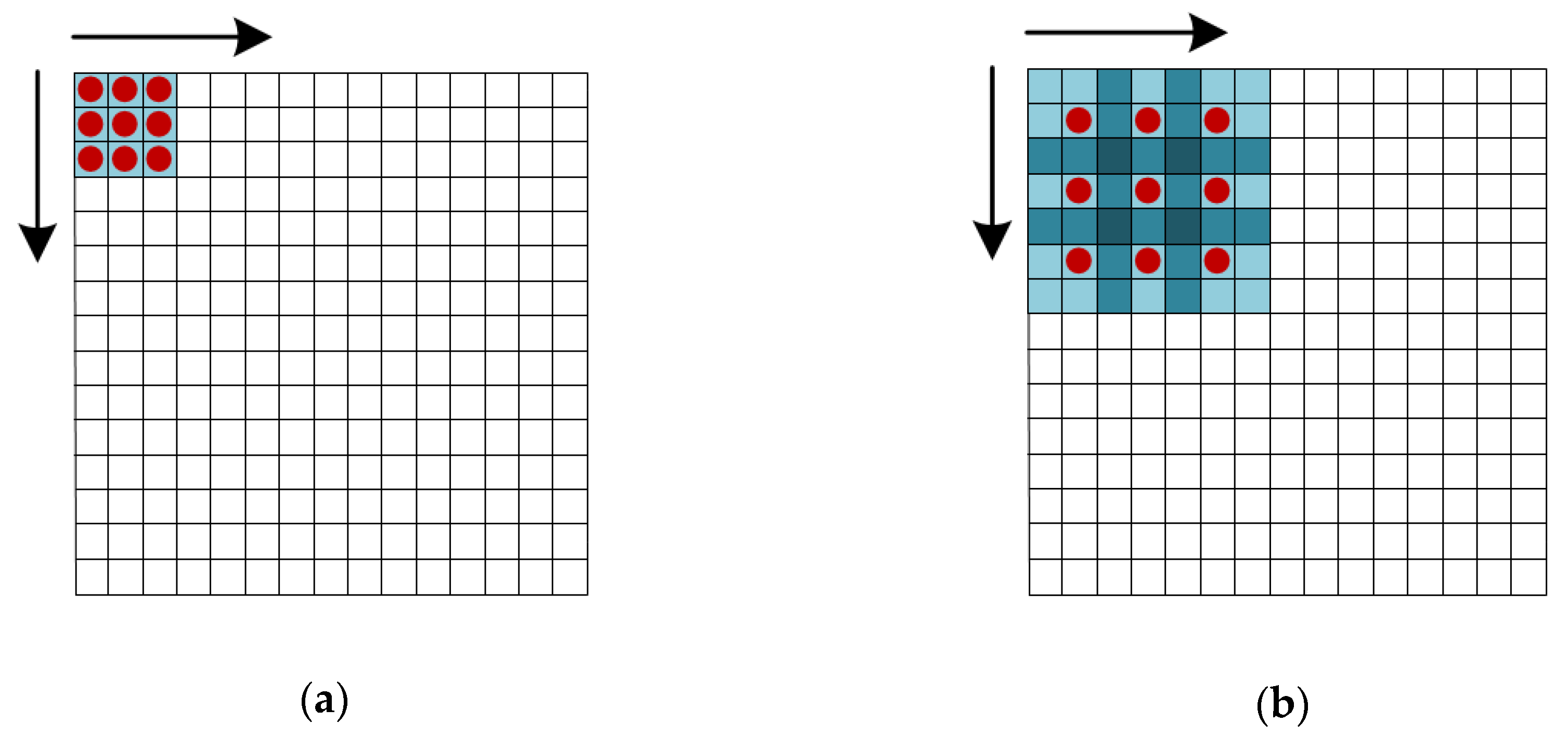
In our paper, dilated convolution is applied to extract features from input layer, which adopts inject holes into traditional convolutional kernels and it can increase the reception field. The difference between standard kernel and dilated kernel is represented in Figure 4. The kernel will slide from left to right, top to bottom on the image. As shown in Figure 4a, the red points are standard kernel. For dilated kernel (see Figure 4b), several inject holes highlighted as blue or dark blue points were added. The values at these points are set as 0. Only values at red points are calculated. Suppose is a discrete filter with the size of , the discrete convolution operator can be defined as
When is a dilation factor, should be defined as
That is the calculation formula of dilated convolution.
2.4.2. Depthwise Separable Convolution with Dilated Kernel
Suppose the size of input tensor is and there is a convolution kernel, the output of this layer would be an tensor when and . The whole process needs parameters and times multiplication.
Depthwise separable convolution decomposes traditional convolution layer into a depthwise convolution and a pointwise convolution. Depthwise process divides the size input tensor into groups. A convolution operation with a kernel is carried out on each group. This process collects the spatial feature of each channel, i.e., depthwise features. The output size output tensor is operated by a traditional convolution kernel, which extract the pointwise feature from each channel. Its output is also a . size tensor. Depthwise and pointwise can be regarded as a convolution layer with much lower amount of computation. The two processes need times multiplication in total.
In order to combine the reception field of dilated convolution with the calculated performance of depthwise separable convolution, we adopt the strategy of adding holes into depthwise convolution kernel in several bottom layers of neural network.
2.4.3. Transposed Convolution
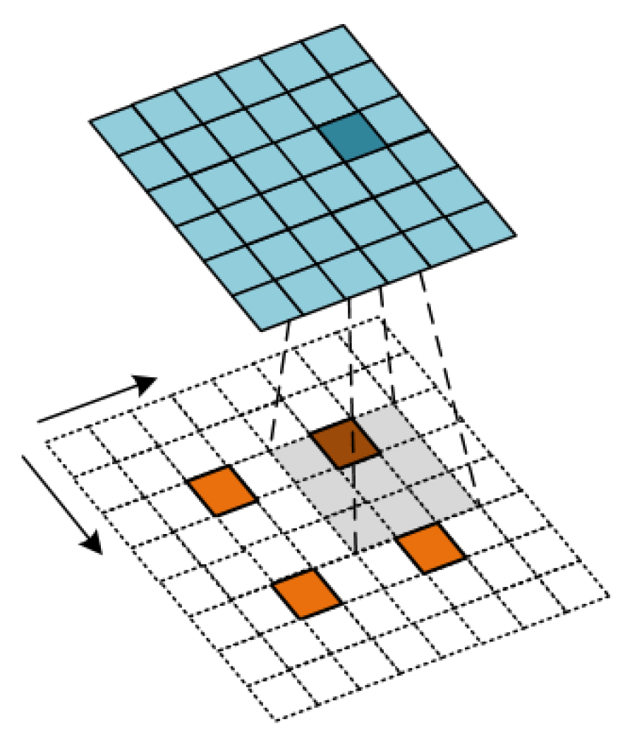
Transposed convolution, also known as deconvolution, is often used as decoder in neural networks. In the semantic segmentation task, transposed convolution upsample the feature map extracted by convolution layer. The final output is a fine classification map with the same size as the original image. In fact, it transposes the convolution kernel in the ordinary convolution we used in the encoder section and inverts the input and output. For example, Figure 5 shows a highly condensed feature map extracted by multilayer network and how it is decoded by a transposed convolution layer. For example, the feature map padded with border of zeros using strides is convolved by a kernel. Its output is a tensor when there is no padding in convolution process.
The detailed parameters of each layer are listed in Table 1. The encoder section contains 10 convolution layers and 2 residual blocks. Convolution layers 1 and 3 adopted depthwise separable convolution, and layer 5 was dilated convolution layer. The decoder section consisted of five deconvolution (transposed convolution) layers, in which layer 1 and layer 2 are connected with convolution layer 7 and layer 3, respectively.
2.4.4. Evaluation Method
MIoU is usually used as an index to measure the accuracy in semantic segmentation task, it is to calculate the intersection between prediction and ground truth. MIoU can be expressed as
which is equivalent to
where TP is the abbreviation for true positive, which means the number of samples when real value and model prediction are both positive. FN represents false negative, which means real value is positive while model prediction is negative. FP represents false positive. is the number of classifications.
3. Experiments and Results
3.1. SAR Data and Preprocessing
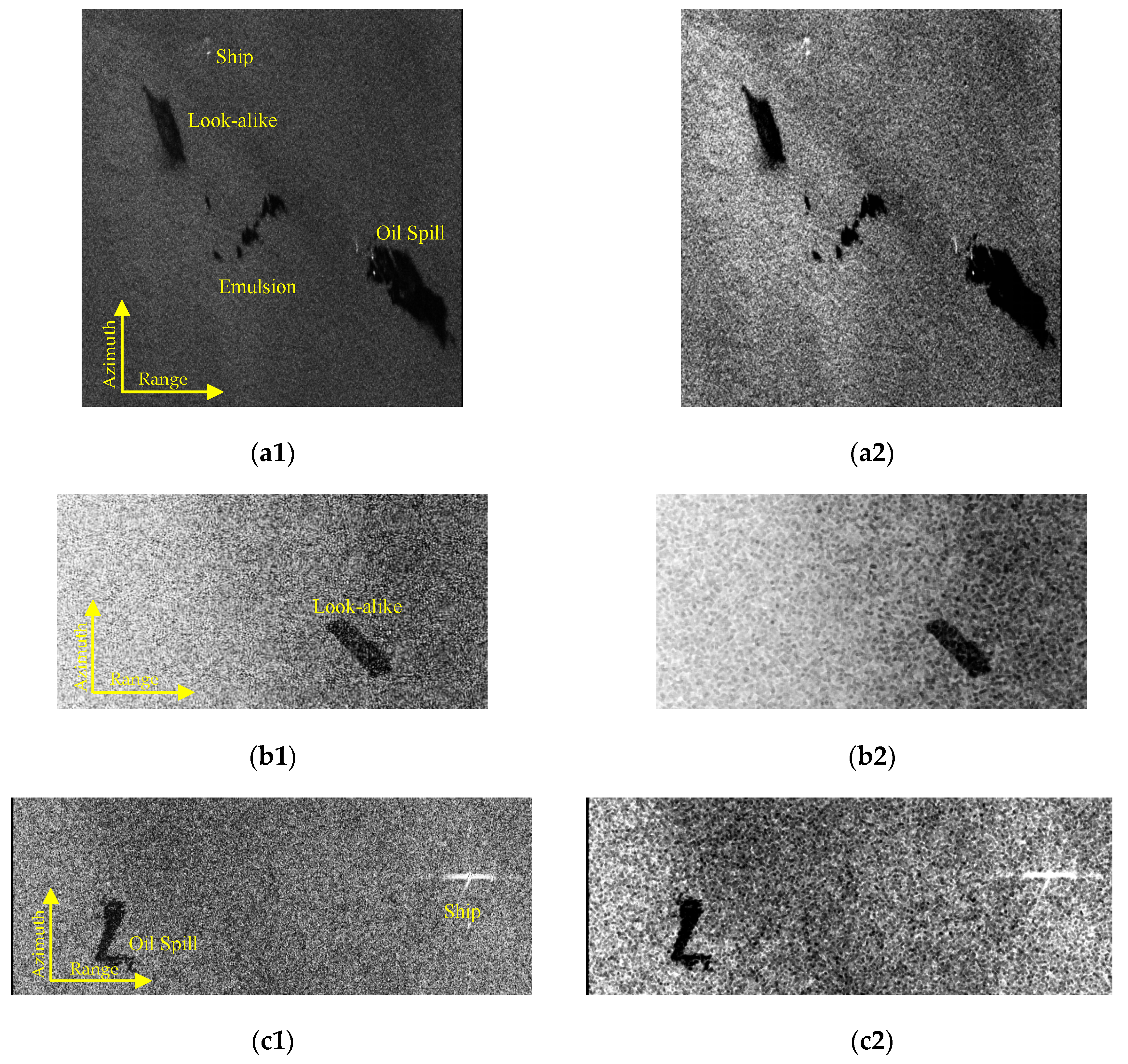
There are three images used in our experiments. Image 1 is a quad-pol oil spill image obtained by C-band Radarsat-2 satellite over the North Sea of England in 2011 during the oil-on-water exercise conducted by the Norwegian Clean Seas Association for Operating Companies (NOFO). The whole image contains five parts in total: clean sea, ships, biogenic look-alike film, emulsion and crude oil spill. The biogenic look-alike film was simulated by Radiagreen plant oil, while emulsion area was composed of Oseberg blend crude oil mixed with 5% IFO380 (Intermediate Fuel Oil). The oil spill area was the Balder crude oil. It was released 9h before SAR acquisition [16]. Emulsions are classified as an independent class in this paper since they have different composition and polarimetric scattering characteristics in SAR images. Image 2 and Image 3 are acquired by C-band SIR-C/X-SAR in 1994, the dark spots contained in images are biogenic look-alike and oil spill, respectively. The biogenic look-alike was composed of Oleyl Alcohol in the experiment [37]. The detailed information of SAR acquisition is listed in Table 2.
The Single Look Complex (SLC) radar images experienced multi-look process and was filtered by Refined Lee Filter. Figure 6 shows the image extract from coherence matrix before and after filtering. It helped suppress speckle noise and enhance the edge of dark spots, and some early experiments have proved that Refined Lee Filter could help increase oil spill detection accuracy.
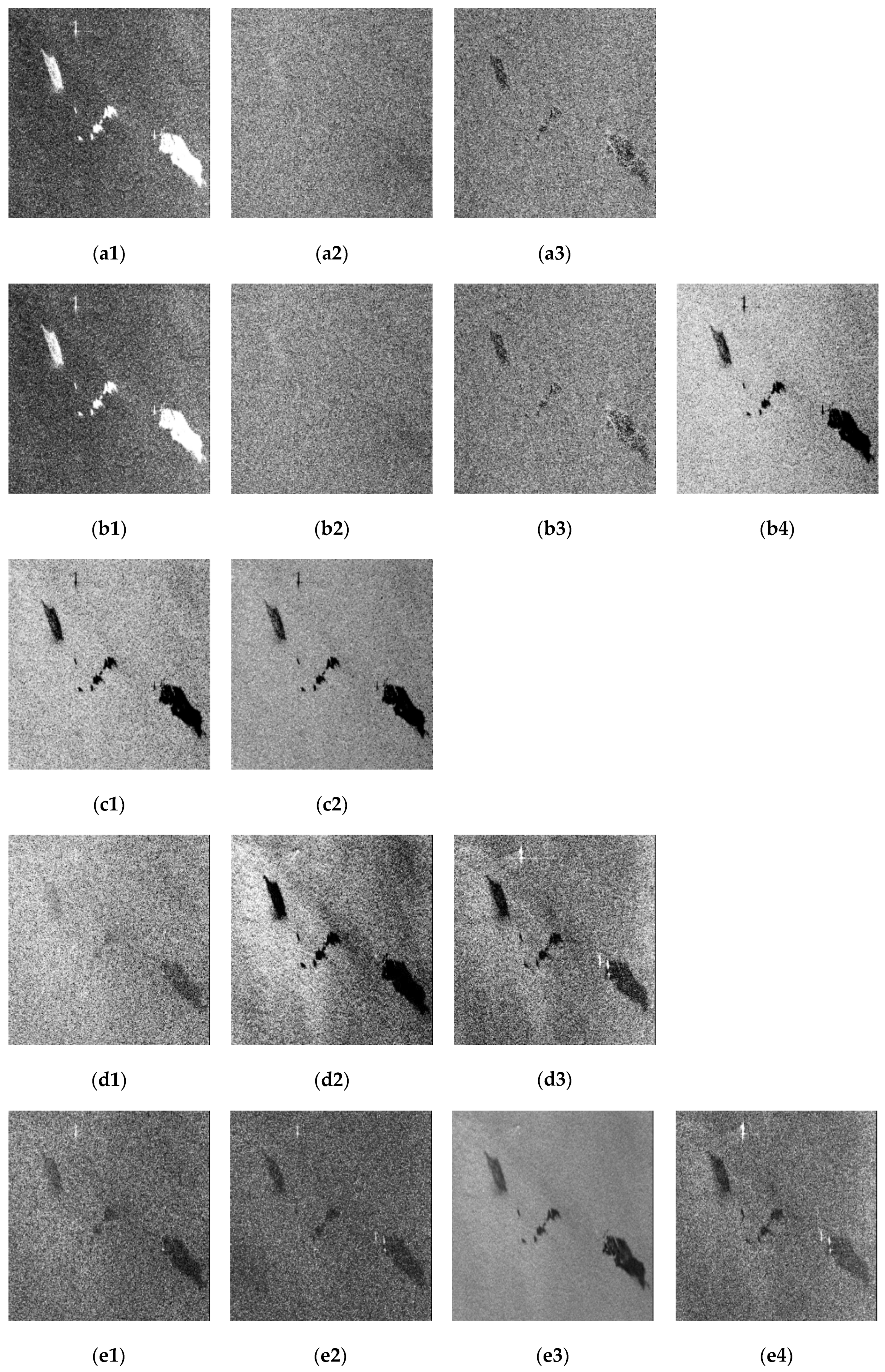
The filtered images were processed by different polarized decomposition methods according to the steps listed in Section 2.2. Figure 7 lists the five groups of polarized parameters extracted from Image 1 as an example: H/A/Alpha, H/A/Alpha/SERD, correlation/conformity coefficients, Freeman decomposition and Yamaguchi decomposition, and characteristics of all these parameters are listed in Table 3.
3.2. SLIC Superpixel Segmentation
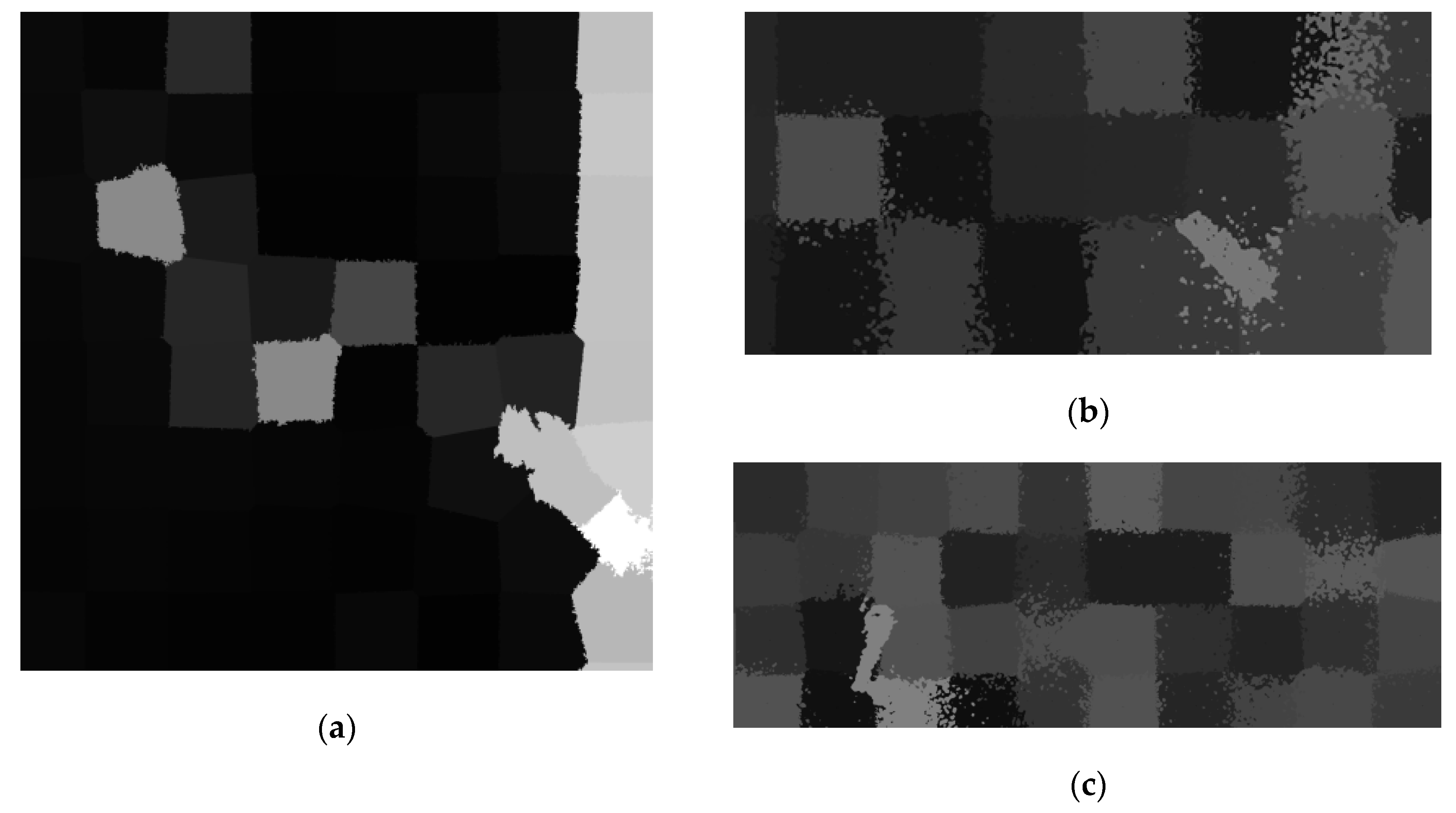
The HH, HV and VV data was taken as input data to perform SLIC superpixel segmentation. We used these three channels of SAR data to generate a new image, it was converted into CIElab color spaces. Following the steps of SCIC superpixel method described in Section 2.3, the superpixel segmentation results of SAR data are shown in Figure 8. The superpixel number of three images was set to 250, 40, 40, respectively. They are another type of input besides polarized parameters for CNN training. It can be seen from Figure 8 that SLIC superpixel divides the image into several independent areas, and can initially locate dark spots, especially in Image 2 and Image 3.
Polarimetric decomposition and superpixel images are divided into five groups as listed in Figure 2. The three SAR images are divided into five categories pixel by pixel: clean sea background (CS), emulsion (EM), biogenic look-alike (LA), oil spill (OS) and ships (SH). All the images are divided into small pictures in the experiment. When multiple parameters are input into CNN, they are stacked along the third axis of images to form a three-dimensional array. The original SAR images only contained 5 ships, in order to increase the number of samples, especially ships, we sampled the same target area for multiple times. We extracted image of target areas from different positions, and these images are divided into 48*48. Thus, we can get several sampling images on the same area. We randomly selected training set and test set from sample images, the number of samples are listed in Table 4. The MIoU was calculated on the test set. They are trained with the proposed network described in Section 2.4 and the output segmentation results are verified with ground truth.
3.3. Oil Spill Classification
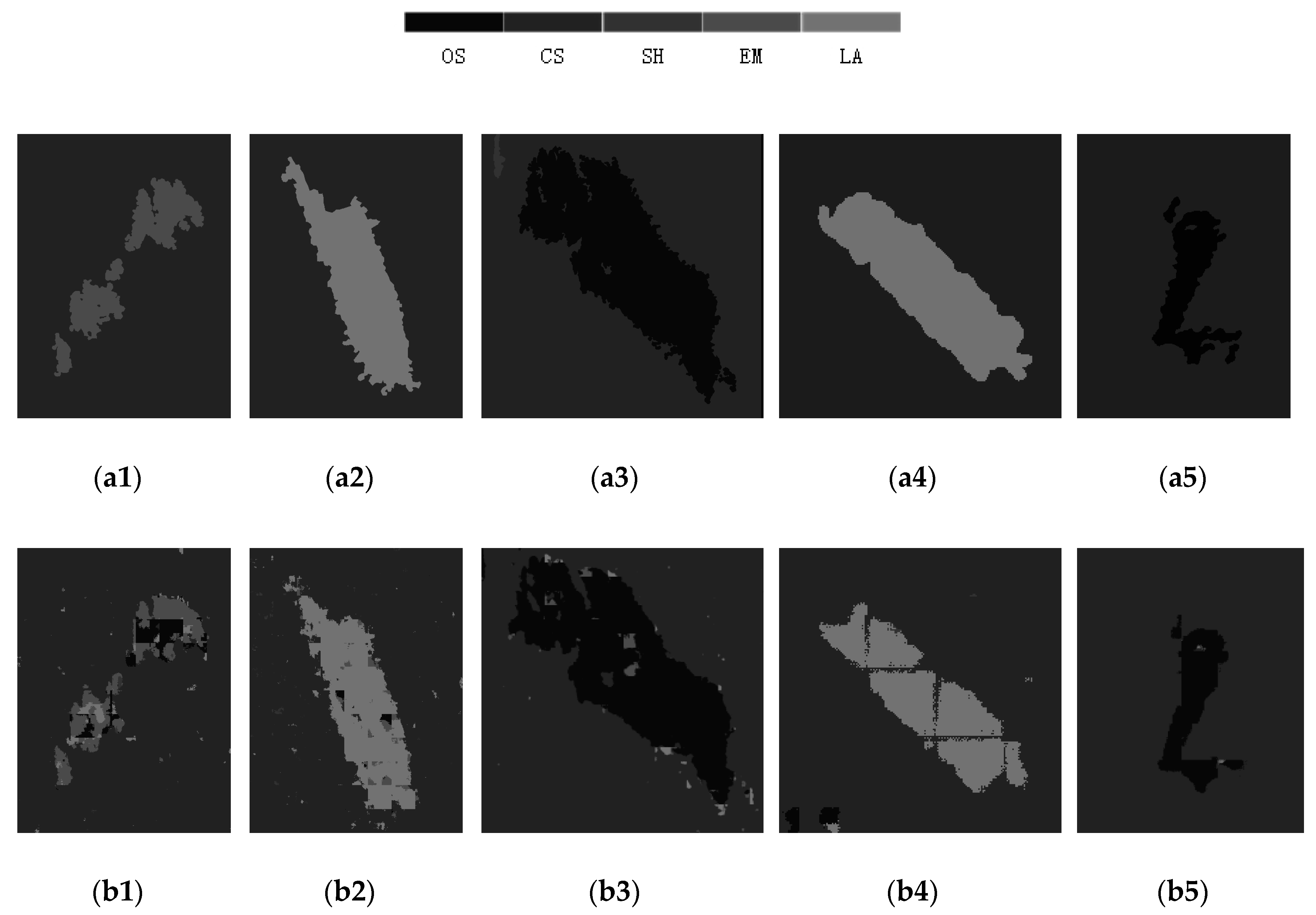
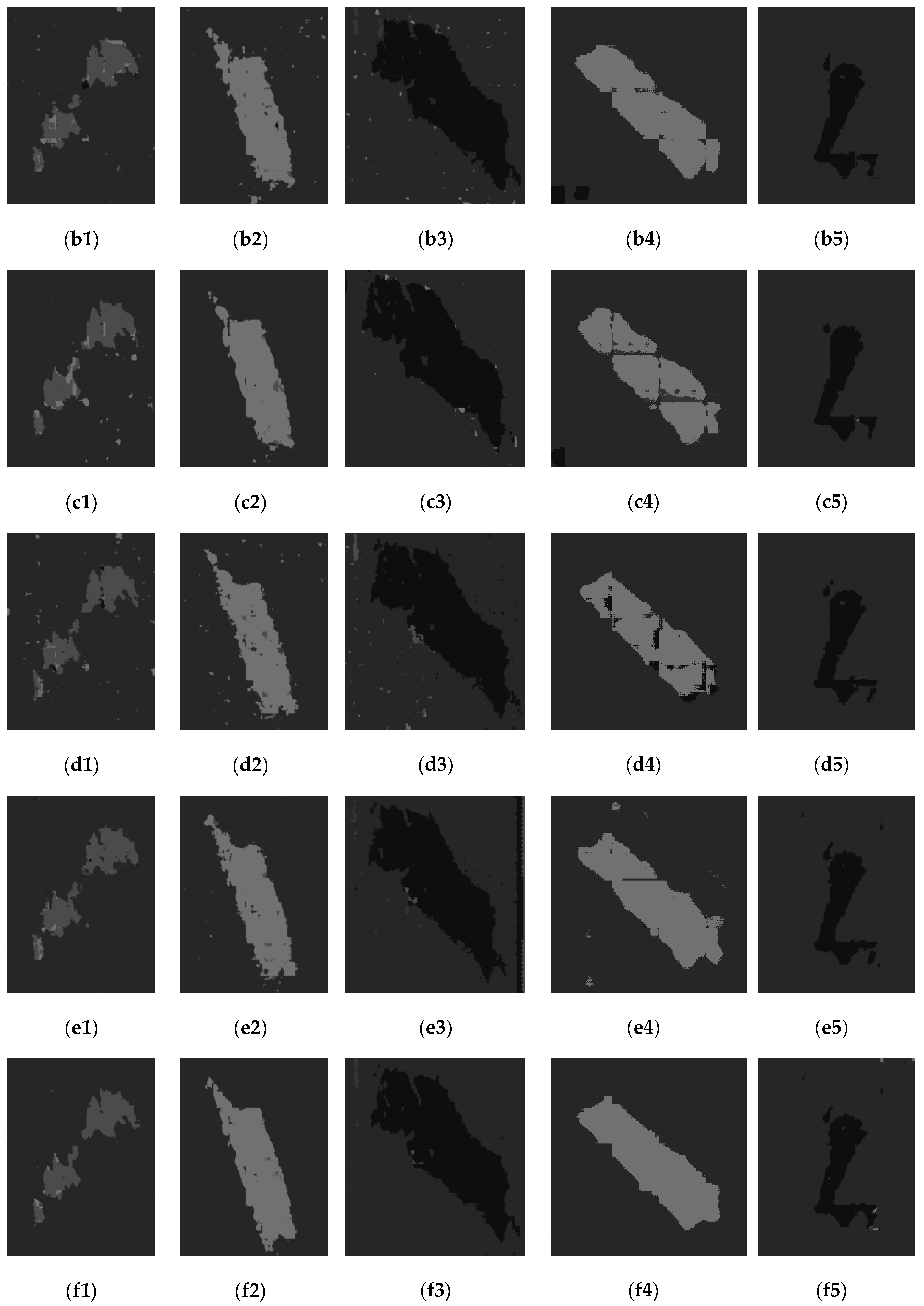
In order to evaluate the influence of SLIC superpixel on segmentation results, we carried out comparative experiments based on each group of polarized parameters with and without superpixel segmentation. Figure 9 presents the segmentation results of five groups of polarized parameters on five dark spots areas of three images. The oil spill area is marked with the dark spots and the light grey means the biogenic look-alikes. The medium grey represents emulsion.
As shown in Figure 9, the dark spots area can be extracted effectively and classified accurately in each group. The classification result of oil spill area in Image 3 showed the best. Among all the polarized decomposition parameters, the performance of Yamaguchi 4-component parameters was the best, followed by Freeman 3-component parameters and H/A/SERD/Alpha. H/A/Alpha could also distinguish each category in the images except ships. The parameter SERD effectively increased the classification accuracy on the basis of H/A/Alpha decomposition. The segmentation result of co-polarized correlation coefficients and conformity coefficients does not perform well nearly in all categories, indicating they are not optimal polarized parameters for detecting oil spill areas.
Considering all categories, the classification results of clean sea (CS) is the best. Then it is followed by oil spill (OS) areas, which is slightly better than look-alikes (LA). The classification accuracy of the categories of emulsions (EM) and ship (SH) are the lowest. The false detection mostly occurred in emulsions. A number of emulsion areas were misclassified into oil spill or look-alikes, especially in the experiments of H/A/Alpha, H/A/SERD/Alpha and co-polarized CC/conformity coefficients. Compared with those results, Freeman 3-component and Yamaguchi 4-component decomposition could distinguish most of these categories successfully. Moreover, the experiment results by applying these two groups of polarized parameters could also detect ships with high reliability, which are almost all misclassified as oil spill areas in other groups’ experimental results.
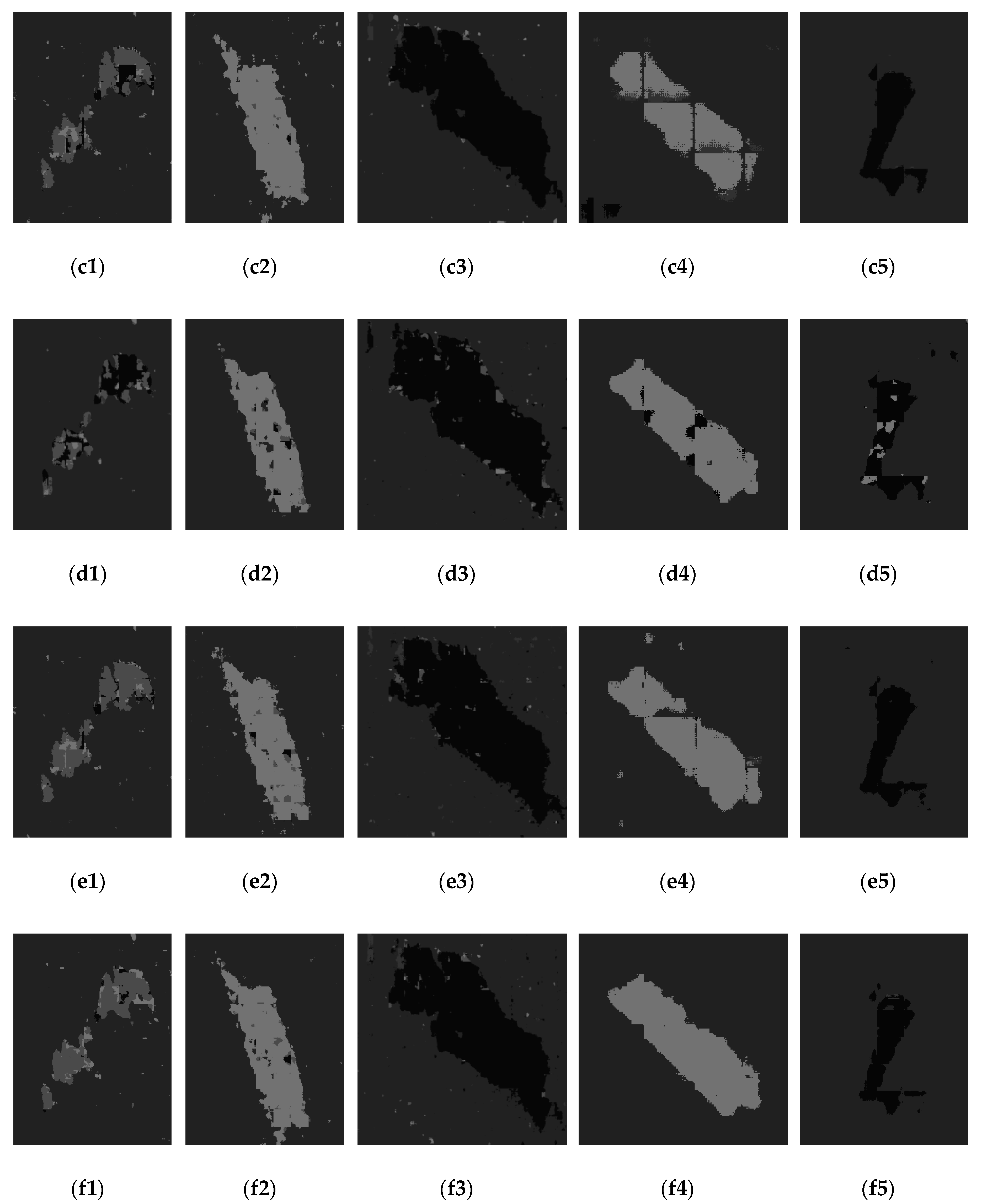
In the followings, we added the SLIC segmentation result from SAR data as another input besides polarized parameters and inputted them together into neural network and repeated the above experiments. The output results are represented in Figure 10. The classification results of each category has been improved significantly, especially for emulsion areas. Compared with the segmentation results without applying superpixel model results, the edge of different classes become more distinct.
The numerical comparison was carried out by calculating the MIoU of each polarized parameter group on the test set. The compared results with and without SLIC superpixel are listed in Table 5. The accuracy of Yamaguchi and Freeman decomposition is significantly higher than other groups of polarized parameters, and that of each classification category has been also improved by SLIC superpixel to varying degree.
For further analysis, Table 6 shows the total MIoU of different polarized parameters decomposition methods. The average MIoU of each classification in all experiments is shown in Table 7. Both Table 6 and Table 7 are calculated from the average value of Table 5. The overall accuracy of different polarimetric parameters after combined with SLIC superpixel segmentation maintained the same trend in previous analysis as illustrated in Table 5 and Table 6. Yamaguchi 4-component decomposition achieved the highest MIoU by 90.5%, followed by Freeman parameters and H/A/SERD/Alpha. Although SLIC superpixel just provide a rough classification of dark spots area, it could also improve MIoU values of each polarimetric parameters, increased by 12.3%, 11.3%, 21.2%, 2.5%, 4.0% relatively. Take Yamaguchi parameters as example, the MIoU of OS area increased from 94.0% to 96.8%, and increased by 0.8%, 12.3% and 9.2% in CS, EM and LA area relatively. What’s more, the largest increase of MIoU occurred in EM area, which increased by 21.9% in average in five groups of polarimetric parameters, as shown in Table 8. CS and OS areas achieved the highest MIoU by 95.9% and 94.1% in all experiments with and without SLIC superpixel, and SH was significantly lower than other parts.
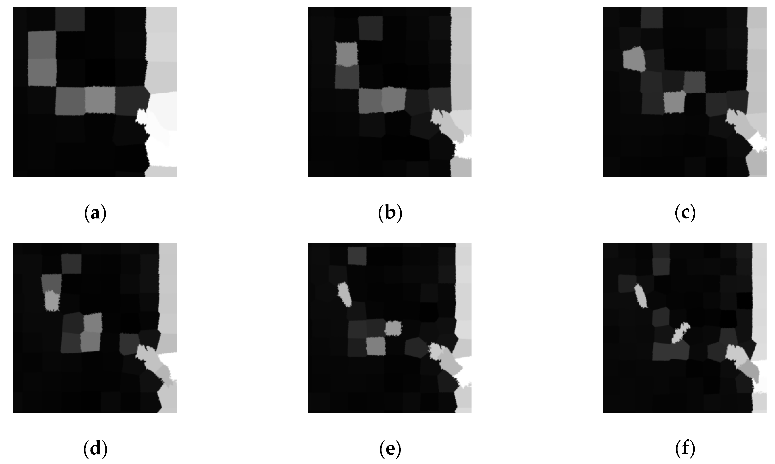
It is worth noting that the number of superpixels in SLIC superpixel segmentation will also affect the final segmentation accuracy. We tested the number of superpixels from 150 to 400 with the step of 50 on Image 1 alone. Figure 11 shows the SLIC segmentation results of different numbers of superpixels. We carried out the comparison experiments with the use of the polarized parameter group of Yamaguchi 4-component decomposition, since it achieved the highest MIoU in the previous experiments. Table 10 lists the MIoU for oil spill segmentation accuracy under different superpixel numbers. The highest accuracy is 91.0% when superpixel number was set to 250.
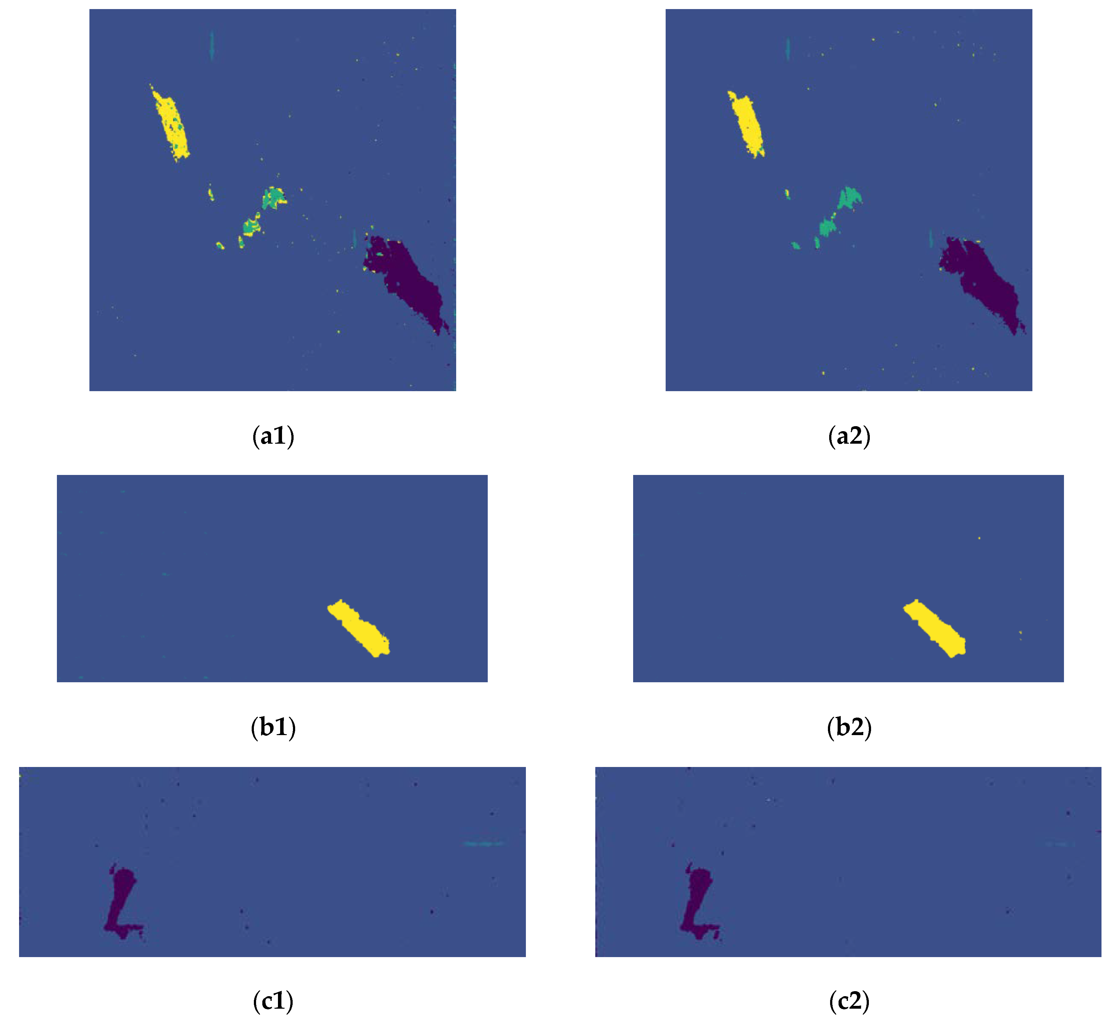
Finally, the classification results of the whole image without and with SLIC superpixel by applying Yamaguchi parameters are represented in Figure 12. Each category on the sea surface can be distinguished with high accuracy. SLIC superpixel helped further improve the accuracy of each category, especially for emulsions. Biogenic look-alikes were also better classified with less misclassification pieces inside. Emulsions can be well detected from oil spill and biogenic look-alike areas, and the segmentation results of other categories also perform better. The improvement effect in Image 1 was the most obvious, while SLIC superpixel mainly helped improve the accuracy of CS area in Image 2 and Image 3.
In order to evaluate the algorithm complexity, we calculate the calculation time of the superpixel segmentation and CNN classification with different polarized parameters, the results are listed in Table 9. Table 10 shows the memory usage of different neural network models. Due to the limitation of experimental conditions, our experiments are carried out on a device without independence GPU. It should be noted that the processing speed will be more than several tens of times faster on a device with independence GPU, hence it will be no problem to achieve near-real time monitoring.
4. Discussion
In order to improve the reception field and reduce parameters, we used depthwise convolution and dilated convolution in several bottom layers of our semantic segmentation model instead of traditional convolution kernel. These strategies achieved high accuracy with small amount of parameters in the experiments.
The emulsion marked in Image 1 we used is mixture of Oseberg oil, IFO380 and water, with water content of approximately 69%. The emulsion has different polarimetric characteristics from oil spill. Actually, they behave in between crude and clean sea surface on polarimetric SAR features. In actual cases, it should be also recognized as a type of oil leakage that will cause damage to ocean environment. The emulsions, biogenic look-alikes and oil spill area are independent of each other in actual SAR images, but dark area in the same test image may be classified into two or more categories. For example, many EM areas are classified into OS or LA as shown in Figure 9.
It was discovered that that parameters calculated from covariance matrix or correlation/conformity coefficients could mistakenly detect the ship as oil spill area. Experiments proved that Yamaguchi and Freeman decomposition parameters performed better in oil spill classification. Both of them are scattering model-based decomposition method, while Yamaguchi decomposition could better deal with the large cross-polarized component caused by complex ground target, which break the reflection symmetry. Hence Yamaguchi decomposition could distinguish each area with relatively high accuracy, especially on ship targets.
Moreover, SLIC can combine neighboring pixels together with special significance and associate adjacent pixels, thus forming connected blocks and greatly improves the classification accuracy, the MIoU of each group polarized parameters has been greatly improved in the demonstrated experiment. Further experiments on Image 1 showed that when superpixel number was set to 250, the recognition accuracy achieved the highest. In fact, the number of superpixels set strongly relies on the type and size of objects. That means that the SLIC superpixel numbers should be adjusted depending on real conditions.
5. Conclusions
In this paper, we proposed an oil spill detection method combining SLIC superpixel model and semantic segmentation algorithm based on CNN. The dilated convolution kernel and depthwise separable convolution kernel was adopted for better computing performance and larger sensing area. SLIC superpixel segmentation is set as an input for the CNN model for auxiliary classification.
The experiments were carried on a C-band fully polarized SAR data of Radarsat-2. We extracted several polarized parameters according to different methods, and tested their performance in oil spill classification based on the proposed method. The results showed that in each group of experiments, this network structure can effectively distinguish the oil spill area and other areas. The highest MIoU value appeared in Yamaguchi decomposition parameters experiment, followed by H/A/SERD/Alpha and Freeman decomposition.
The introduction of SLIC superpixel greatly improved the recognition accuracy. The MIoU values of each group are improved, and their numerical order of the polarimetric feature sets is almost the same as in experiments without SLIC superpixel. Hence, it is suggested that Yamaguchi parameters combined with superpixel segmentation is the most suitable method for oil spill detection.
Author Contributions
Funding acquisition, Q.L., J.W. and Y.L.; methodology, Q.L.; supervision, Q.L., H.F. and J.L.; writing—original draft, J.Z.; writing—review and editing, Q.L., Y.L. and J.W. All authors have read and agreed to the published version of the manuscript.
Acknowledgments
The RADARSAT-2 data in this paper is provided by Canadian Space Agency and MacDonald, Dettwiler and Associates. The authors are very thankful to the partially support of the National Natural Science Foundation of China (grant No. 41601446, 41706201 and 41801284).
Conflicts of Interest
The authors declare no conflict of interest.
References
- Migliaccio, M.; Nunziata, F.; Montuori, A. A Multifrequency Polarimetric SAR Processing Chain to Observe Oil Fields in the Gulf of Mexico. IEEE Trans. Geosci. Remote Sens. 2011, 49, 4729–4737. [Google Scholar] [CrossRef]
- Alpers, W.; Holt, B.; Zeng, K. Oil spill detection by imaging radars: Challenges and pitfalls. Remote Sens. Environ. 2017, 201, 133–147. [Google Scholar] [CrossRef]
- Solberg, S.; Storvik, G.; Solberg, R.; Volden, E. Automatic Detection of Oil Spills in ERS SAR Images. IEEE Trans. Geosci. Remote Sens. 1999, 37, 1916–1924. [Google Scholar] [CrossRef] [Green Version]
- Garcia-Pineda, O.; MacDonald, R.; Li, X.; Jackson, C.R.; Pichel, W.G. Oil Spill Mapping and Measurement in the Gulf of Mexico with Textual Classifier Neural Network Algorithm. IEEE J. Sel. Top. Appl. Earth Obs. Remote Sens. 2013, 6, 2517–2525. [Google Scholar] [CrossRef]
- Solberg, S.; Brekke, C.; Husoy, O. Oil Spill Detection in Radarsat and Envisat SAR Images. IEEE Trans. Geosci. Remote Sens. 2007, 45, 746–755. [Google Scholar] [CrossRef]
- Yang, C.-S.; Kim, Y.-S.; Ouchi, K.; Na, J.-H. Comparison with L-, C-, and X-band real SAR images and simulation SAR images of spilled oil on sea surface. In Proceedings of the 2009 IEEE International Geoscience and Remote Sensing Symposium, IGARSS 2009, Cape Town, South Africa, 12–17 July 2009; pp. 673–676. [Google Scholar]
- Wismann, V. Radar Signatures of Mineral Oil Spills Measured by an Airborne Multi-Frequency Radar and the ERS-1 SAR. In Proceedings of the 1993 IEEE International Geoscience and Remote Sensing Symposium, IGARSS 1993, Tokyo, Japan, 18–21 August 1993; pp. 940–942. [Google Scholar]
- Cheng, Y.; Liu, B.Q.; Li, X.; Nunziata, F.; Xu, Q.; Ding, X.; Migliaccio, M.; Pichel, W.G. Monitoring of Oil Spill Trajectories with COSMO-SkyMed X-Band SAR Images and Model Simulation. IEEE J. Sel. Top. Appl. Earth Obs. Remote Sens. 2014, 7, 2895–2901. [Google Scholar] [CrossRef]
- Fingas, M.; Brown, E. A Review of Oil Spill Remote Sensing. Sensors 2018, 18, 91. [Google Scholar] [CrossRef] [Green Version]
- Collins, J.; Denbina, M.; Minchew, B.; Jones, C.E.; Holt, B. On the Use of Simulated Airborne Compact Polarimetric SAR for Characterizing Oil-Water Mixing of the Deepwater Horizon Oil Spill. IEEE J. Sel. Top. Appl. Earth Obs. Remote Sens. 2015, 8, 1062–1077. [Google Scholar] [CrossRef]
- Li, H.; Perrie, W.; He, Y.; Wu, J.; Luo, X. Analysis of the Polarimetric SAR Scattering Properties of Oil-Covered Waters. IEEE J. Sel. Top. Appl. Earth Obs. Remote Sens. 2015, 8, 3751–3759. [Google Scholar] [CrossRef]
- Freeman, A.; Durden, L. A Three-Component Scattering Model for Polarimetric SAR Data. IEEE Trans. Geosci. Remote Sens. 1998, 36, 963–973. [Google Scholar] [CrossRef] [Green Version]
- Yamaguchi, Y.; Moriyama, T.; Ishido, M.; Yamada, H. Four-Component Scattering Model for Polarimetric SAR Image Decomposition. IEEE Trans. Geosci. Remote Sens. 2005, 43, 1699–1706. [Google Scholar] [CrossRef]
- Cloude, R.; Pottier, E. An Entropy Based Classification Scheme for Land Applications of Polarimetric SAR. IEEE Trans. Geosci. Remote Sens. 1997, 35, 68–78. [Google Scholar] [CrossRef]
- Allain, S.; Lopez-Martinez, C.; Ferro-Famil, L.; Pottier, E. New Eigenvalue-based Parameters for Natural Media Characterization. In Proceedings of the 2005 IEEE International Geoscience and Remote Sensing Symposium, IGARSS 2005, Seoul, Korea, 29–29 July 2005; pp. 40–43. [Google Scholar]
- Skrunes, S.; Brekke, C.; Eltoft, T. Characterization of Marine Surface Slicks by Radarsat-2 Multipolarization Features. IEEE Trans. Geosci. Remote Sens. 2014, 52, 5302–5319. [Google Scholar] [CrossRef] [Green Version]
- Chen, G.; Li, Y.; Sun, G.; Zhang, Y. Application of Deep Networks to Oil Spill Detection Using Polarimetric Synthetic Aperture Radar Images. Appl. Sci. 2017, 7, 968. [Google Scholar] [CrossRef]
- Zhang, Y.; Li, Y.; Liang, X.S.; Tsou, J. Comparison of Oil Spill Classifications Using Fully and Compact Polarimetric SAR Images. Appl. Sci. 2017, 7, 193. [Google Scholar] [CrossRef] [Green Version]
- He, K.; Zhang, X.; Ren, S.; Sun, J. Deep Residual Learning for Image Recognition. Available online: https://arxiv.org/abs/1512.03385v1 (accessed on 10 December 2015).
- Hadji, I.; Wildes, P. What Do We Understand About Convolutional Networks? Available online: https://arxiv.org/abs/1803.08834v1 (accessed on 23 May 2018).
- Yang, Y.; Zhong, Z.; Shen, T.; Lin, Z. Convolutional Neural Networks with Alternatively Updated Clique. In Proceedings of the 2018 IEEE/CVF Conference on Computer Vision and Pattern Recognition, Salt Lake City, UT, USA, 18–22 June 2018. [Google Scholar]
- Lin, M.; Chen, Q.; Yan, S. Network in Network. In Proceedings of the ICLR2014 International Conference on Learning Representations, Banff, AB, Canada, 14–16 April 2014. [Google Scholar]
- Howard, G.; Zhu, M.; Chen, B.; Kalenichenko, D.; Wang, W. MobileNets: Efficient Convolutional Neural Networks for Mobile Vision Applicatoins. Available online: https://arxiv.org/abs/1704.04861 (accessed on 17 April 2017).
- Howard, A.; Sandler, M.; Chu, G.; Chen, L.; Chen, B. Searching for MobileNetV3. Available online: https://arxiv.org/abs/1905.02244 (accessed on 6 May 2019).
- Long, J.; Shelhamer, E.; Darrell, T. Fully Convolutional Networks for Semantic Segmentation. In Proceedings of the 2015 IEEE/CVF Conference on Computer Vision and Pattern Recognition, Boston, MA, USA, 7–12 June 2015. [Google Scholar]
- Yu, F.; Koltun, V. Multi-Scale Context Aggregation by Dialted Convolutions. In Proceedings of the International Conference on Learning Representations 2016, San Juan, Puerto Rico, 2–4 May 2016. [Google Scholar]
- Garcia-Garcia, A.; Orts-Escolano, S.; Opera, S.O.; Villena-Martinez, V.; Garcia-Rodriguez, J. A Review on Deep Learning Techniques Applied to Semantic Segmentation. Available online: https://arxiv.org/abs/1704.06857 (accessed on 22 April 2018).
- Chen, L.-C.; Zhu, Y.; Papandreou, G.; Schroff, F.; Adam, H. Encoder-Decoder with Atrous Separable Convolution for Semantic Image Segmentation. Available online: https://arxiv.org/abs/1802.02611v3 (accessed on 22 August 2018).
- Krestenitis, M.; Orfanids, G.; Ioannidis, K.; Avgerinakis, K.; Vrochidis, S.; Kompatsiaris, I. Oil Spill Identification from Satellite Images Using Deep Neural Networks. Remote Sens. 2019, 11, 1762. [Google Scholar] [CrossRef] [Green Version]
- Yu, X.; Zhang, H.; Luo, C.; Qi, H.; Ren, P. Oil Spill Segmentation via Adversarial f-Divergence Learning. IEEE Trans. Geosci. Remote Sens. 2018, 56, 4973–4988. [Google Scholar] [CrossRef]
- Kim, D.; Jung, H.-S. Mapping Oil Spills from Dual-Polarized SAR Images Using an Artificial Neural Network: Application to Oil Spill in the Kerch Strait in November 2007. Sensors 2018, 18, 2237. [Google Scholar] [CrossRef] [Green Version]
- Ren, X.; Malik, J. Learning a Classification Model for Segmentation. In Proceedings of the ICCV 2003 IEEE International Conference on Computer Vision, Nice, France, 13–16 October 2003; Volume 1, pp. 10–17. [Google Scholar]
- Achanta, R.; Shaji, A.; Smith, K.; Lucchi, A.; Fua, P.; Süsstrunk, S. SLIC Superpixels Compared to State-of-the-art Superpixel Methods. IEEE Trans. Pattern Anal. Mach. Intell. 2012, 34, 2274–2282. [Google Scholar] [CrossRef] [Green Version]
- Bovenga, F.; Derauw, D.; Rana, F.M.; Barbier, C.; Refice, A.; Veneziani, N.; Vitulli, R. Multi-Chromatic Analysis of SAR Images for Coherent Target Detection. Remote Sens. 2014, 6, 8822–8843. [Google Scholar] [CrossRef] [Green Version]
- Bovenga, F.; Derauw, D.; Barbier, C.; Rana, F.M.; Refice, A.; Veneziani, N.; Vitulli, R. Multi-Chromatic Analysis of SAR Images for Target Analysis. In Proceedings of the Conference on SAR Image Analysis, Modeling, and Techniques, Dresden, Germany, 24–26 September 2013. [Google Scholar]
- Salberg, A.; Larsen, S. Classification of Ocean Surface Slicks in Simulated Hybrid-Polarimetric SAR Data. IEEE Trans. Geosci. Remote Sens. 2018, 56, 7062–7073. [Google Scholar] [CrossRef]
- Nunziata, M. Single- and Multi-Polarization Electromagnetic Models for SAR Sea Oil Slick Observation. Ph.D. Thesis, Parthenope University of Naples, Naples, Italy, December 2008. [Google Scholar]
Figure 1.
Flow chart of our oil spill detection method.

Figure 2.
Structure of neural networks in our segmentation method. Blue and green blocks donate encoder parts, which consist of multi convolution layers, here we used depthwise separable convolution, dilated convolution and standard convolution as filter kernel, respectively. Purple-red blocks constitute the decoder part, it outputs a classification map with the same size as original image.

Figure 3.
Polarized parameters extraction. We extracted 13 polarized parameters in total. They are divided into five groups as the position of the box in the figure, each group was input into neural network for classification.
Figure 3.
Polarized parameters extraction. We extracted 13 polarized parameters in total. They are divided into five groups as the position of the box in the figure, each group was input into neural network for classification.

Figure 4.
Convolution kernels for (a) standard kernel, which has a receptive filed of , and (b) dilated kernel with dilation rate = 2, and its receptive field is .
Figure 4.
Convolution kernels for (a) standard kernel, which has a receptive filed of , and (b) dilated kernel with dilation rate = 2, and its receptive field is .

Figure 5.
Convolution process of transposed convolution layer.

Figure 6.
Three oil spill data used in the experiments. Left side shows the original image, and right side are images processed by Refined Lee Filter. (a1,a2) Image 1 acquired by Radarsat-2, (b1,b2) Image 2 (PR11588) acquired by SIR-C/X-SAR and (c1,c2) Image 3 (PR44327) acquired by Spaceborne Imaging Radar-C/X-Band Synthetic Aperture Radar (SIR-C/X-SAR).

Figure 7.
All the polarized features extracted from Radarsat2 data. (a1–a3) H/A/Alpha decomposition, a1 for entropy, a2 for anisotropy, a3 for alpha. (b1–b4) H/A/Alpha decomposition and Single-Bounce Eigenvalue Relative Difference (SERD), b1 for entropy, b2 for anisotropy, b3 for alpha, b4 for SERD. (c1,c2) Scattering coefficients calculated from scattering matrix, c1 for co-polarized correlation coefficients, c2 for conformity coefficients. (d1–d3) Freeman 3-component decomposition, d1 for double-bounce scattering, d2 for rough surface scattering, d3 for volume scattering. (e1–e4) Yamaguchi 4-component decomposition, e1 for double-bounce scattering, e2 for helix scattering, e3 for rough surface scattering, e4 for volume scattering.

Figure 8.
Simple Linear Iterative Clustering (SLIC) superpixel segmentation results. (a) Image 1, (b) Image 2 and (c) Image 3.
Figure 8.
Simple Linear Iterative Clustering (SLIC) superpixel segmentation results. (a) Image 1, (b) Image 2 and (c) Image 3.

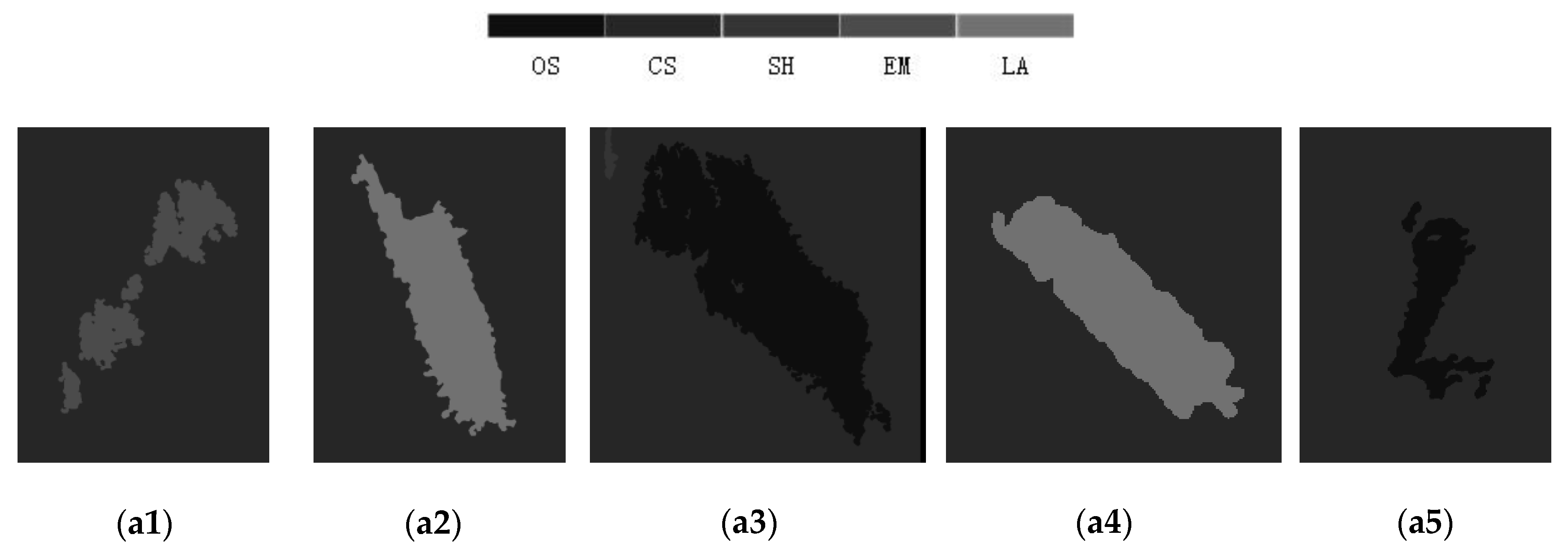
Figure 9.
The results of dark spots area verified by polarized parameters, 1-3 in each group represents emulsion, 2 for biogenic look-alike, 3 for oil-spill area of Image 1, 4 and 5 represent biogenic look alike and oil spill area of Image 2 and Image 3. (a1–a5) Ground truth, (b1–b5) H/A/Alpha, (c1–c5) H/A/SERD/Alpha, (d1–d5) Scattering Coefficients, (e1–e5) Freeman 3-Component Decomposition, (f1–f5) Yamaguchi 4-Component Decomposition.


Figure 10.
The results of dark spots area verified by polarized parameters combined with SLIC superpixel segmentation, 1-3 in each group represents emulsion, 2 for biogenic look-alike, 3 for oil-spill area of Image 1. Images 4 and 5 represent biogenic look-alike and oil spill area of Image 2 and Image 3. (a1–a5) Ground truth, (b1–b5) H/A/Alpha, (c1–c5) H/A/SERD/Alpha, (d1–d5) Scattering Coefficients, (e1–e5) Freeman 3-Component Decomposition, (f1–f5) Yamaguchi 4-Component Decomposition.


Figure 11.
SLIC superpixel segmentation results with different superpixel numbers. (a) 150, (b) 200, (c) 250, (d) 300, (e) 350, (f) 400.
Figure 11.
SLIC superpixel segmentation results with different superpixel numbers. (a) 150, (b) 200, (c) 250, (d) 300, (e) 350, (f) 400.

Figure 12.
The whole classification result of Yamaguchi 4-component parameters. Left: the results without SLIC superpixel; right: the results with SLIC superpixel. (a1,a2) Image 1, (b1,b2) Image 2, (c1,c2) Image 3.
Figure 12.
The whole classification result of Yamaguchi 4-component parameters. Left: the results without SLIC superpixel; right: the results with SLIC superpixel. (a1,a2) Image 1, (b1,b2) Image 2, (c1,c2) Image 3.


Table 1.
The detailed parameters of segmentation networks.
| Layer 1 | Filter | Kernel Size | Strides |
|---|---|---|---|
| Conv 1 | depthwise | 1 | |
| Conv 2 | Conv | 2 | |
| Conv 3 | depthwise | 1 | |
| Conv 4 | Conv | 2 | |
| Conv 5 | dilated | 1 | |
| Conv 6 | Conv | 2 | |
| Conv 7 | Conv | 2 | |
| Conv 8 | Conv | 1 | |
| Conv 9 | Conv | 3 | |
| Conv 10 | Conv | 1 | |
| Res 1 | Conv | 4 | |
| Res 2 | Conv | 4 | |
| Deconv 1 | transposed | 1 | |
| Deconv 2 | transposed | 8 | |
| Deconv 2_1 | transposed | 4 | |
| Deconv 3 | transposed | 2 | |
| Deconv 3_1 | transposed | 2 |
1 Conv, Res and Deconv represent the blue, green and purple-red blocks, respectively.
Table 2.
Details of Synthetic Aperture Radar (SAR) image acquisition.
| Image ID | 137348 | PR11588 | PR44327 |
|---|---|---|---|
| Radar Sensor | Radarsat-2 | SIR-C/X-SAR | SIR-C/X-SAR |
| SAR Band | C | C | C |
| Pixel Spacing (m) | |||
| Radar Center Frequency (Hz) | |||
| Centre Incidence Angle (deg) | 35.287144 | 23.600 | 45.878 |
Table 3.
Characteristics of polarized parameters in experiments.
| Parameter | Clean Sea | Look alike | Emulsion | Oil Spill | Ship |
|---|---|---|---|---|---|
| Entropy | low | high | higher | higher | higher |
| Anisotropy | low | low | low | low | low |
| Alpha | low | lower | low | low | low |
| SERD | high | low | lower | lower | lower |
| Correlation Coefficient | high | low | lower | lower | lower |
| Conformity Coefficient | high | low | lower | lower | lower |
| Freeman Double-Bounce | high | low | low | lower | higher |
| Freeman Rough-Surface | high | low | low | low | higher |
| Freeman Volume | high | lower | lower | low | higher |
| Yamaguchi Double-Bounce | high | low | low | lower | higher |
| Yamaguchi Helix | low | lower | lower | lower | high |
| Yamaguchi Rough-Surface | high | low | lower | lower | higher |
| Yamaguchi Volume | high | lower | lower | low | higher |
Table 4.
Number of samples of each category.
| Areas | CS | EM | LA | OS | SH |
| Training set | 80 | 75 | 82 | 88 | 31 |
| Test set | 27 | 25 | 28 | 30 | 12 |
Table 5.
Mean Intersection over Union (MIoU) result on each classification of polarized parameters experiments.
Table 5.
Mean Intersection over Union (MIoU) result on each classification of polarized parameters experiments.
| Without SLIC Superpixel | With SLIC Superpixel | |||||||||
|---|---|---|---|---|---|---|---|---|---|---|
| Classification | CS | EM | LA | OS | SH | CS | EM | LA | OS | SH |
| H/A/Alpha | 94.0% | 70.8% | 84.2% | 85.7% | 10.5% | 95.6% | 88.3% | 89.7% | 93.4% | 39.7% |
| H/A/SERD/Alpha | 94.5% | 80.7% | 84.9% | 88.3% | 11.7% | 95.8% | 91.0% | 91.7% | 95.1% | 43.1% |
| Scattering coefficients 1 | 94.1% | 27.3% | 82.3% | 80.2% | 6.8% | 94.7% | 85.8% | 84.2% | 90.1% | 41.5% |
| Freeman | 95.8% | 80.7% | 82.4% | 90.6% | 60.7% | 96.3% | 91.1% | 91.5% | 95.1% | 48.3% |
| Yamaguchi | 96.1% | 81.8% | 85.4% | 94.0% | 75.0% | 96.9% | 94.1% | 94.6% | 96.8% | 70.2% |
1 scattering coefficient means the combination of correlation coefficients and conformity coefficients.
Table 6.
Total MIoU results of each group of polarimetric parameters.
| Parameters | H/A/Alpha | H/A/SERD/Alpha | Scattering coefficients | Freeman | Yamaguchi |
| Without SLIC Superpixel | 69.0% | 72.0% | 58.1% | 82.0% | 86.5% |
| With SLIC Superpixel | 81.3% | 83.3% | 79.3% | 84.5% | 90.5% |
Table 7.
Average MIoU of each classification.
| Areas | CS | EM | LA | OS | SH |
| Without SLIC Superpixel | 94.9% | 68.2% | 83.8% | 87.8% | 32.9% |
| With SLIC Superpixel | 95.9% | 90.1% | 90.3% | 94.1% | 48.6% |
Table 8.
Total MIoU results of Yamaguchi parameters combined with different SLIC parameters.
| Superpixels | 150 | 200 | 250 | 300 | 350 | 400 |
|---|---|---|---|---|---|---|
| Total MIoU | 87.1% | 88.5% | 91.0% | 90.3% | 90.5% | 86.6% |
Table 9.
Calculation time of each process (seconds).
| Image 1 | Image 2 | Image 3 | ||
|---|---|---|---|---|
| Pixel Number in Experiments | ||||
| Computer Configuration | i5-8250u CPU 8GB | |||
| Superpixel Segmentation(s) | 1742 | 576 | 482 | |
| CNN Classification with SLIC(s) | H/A/Alpha | 1594 | 135 | 243 |
| H/A/Alpha/SERD | 2107 | 186 | 359 | |
| Scattering Coefficients | 1023 | 102 | 159 | |
| Freeman | 1602 | 133 | 245 | |
| Yamaguchi | 2115 | 192 | 361 | |
Table 10.
Memory Usage Condition of CNN.
| Without SLIC | With SLIC | |
|---|---|---|
| H/A/Alpha | 59.2 M | 91.3 M |
| H/A/Alpha/SERD | 91.3 M | 130 M |
| Scattering Coefficients | 33.9 M | 59.2 M |
| Freeman | 59.2 M | 91.3 M |
| Yamaguchi | 91.3 M | 130 M |
© 2020 by the authors. Licensee MDPI, Basel, Switzerland. This article is an open access article distributed under the terms and conditions of the Creative Commons Attribution (CC BY) license (http://creativecommons.org/licenses/by/4.0/).
Share and Cite
MDPI and ACS Style
Zhang, J.; Feng, H.; Luo, Q.; Li, Y.; Wei, J.; Li, J. Oil Spill Detection in Quad-Polarimetric SAR Images Using an Advanced Convolutional Neural Network Based on SuperPixel Model. Remote Sens. 2020, 12, 944. https://doi.org/10.3390/rs12060944
AMA Style
Zhang J, Feng H, Luo Q, Li Y, Wei J, Li J. Oil Spill Detection in Quad-Polarimetric SAR Images Using an Advanced Convolutional Neural Network Based on SuperPixel Model. Remote Sensing. 2020; 12(6):944. https://doi.org/10.3390/rs12060944
Chicago/Turabian StyleZhang, Jin, Hao Feng, Qingli Luo, Yu Li, Jujie Wei, and Jian Li. 2020. "Oil Spill Detection in Quad-Polarimetric SAR Images Using an Advanced Convolutional Neural Network Based on SuperPixel Model" Remote Sensing 12, no. 6: 944. https://doi.org/10.3390/rs12060944
Note that from the first issue of 2016, this journal uses article numbers instead of page numbers. See further details here.