Feedback Unilateral Grid-Based Clustering Feature Matching for Remote Sensing Image Registration
by
Zhaohui Zheng
1,2, 
Hong Zheng
1,
Yong Ma
1,
Fan Fan
1,*,
Jianping Ju
1,3,
Bichao Xu
4,
Mingyu Lin
3 and
Shuilin Cheng
5 1
School of Electronic Information, Wuhan University, Wuhan 430079, China
2
Department of Public Courses, Wuhan Railway Vocational College of Technology, Wuhan 430205, China
3
School of Mechanical & Electrical and Information Engineering, Hubei Business College, Wuhan 430000, China
4
Wuhan Institute of Virology, Chinese Academy of Sciences, Wuhan 430000, China
5
School of Statistics and Mathematics, Zhongnan University of Economics and Law, Wuhan 430000, China
*
Author to whom correspondence should be addressed.
Remote Sens. 2019, 11(12), 1418; https://doi.org/10.3390/rs11121418
Submission received: 27 April 2019
/
Revised: 10 June 2019
/
Accepted: 10 June 2019
/
Published: 14 June 2019
(This article belongs to the Special Issue Robust Multispectral/Hyperspectral Image Analysis and Classification)
Abstract
:In feature-based image matching, implementing a fast and ultra-robust feature matching technique is a challenging task. To solve the problems that the traditional feature matching algorithm suffers from, such as long running time and low registration accuracy, an algorithm called feedback unilateral grid-based clustering (FUGC) is presented which is able to improve computation efficiency, accuracy and robustness of feature-based image matching while applying it to remote sensing image registration. First, the image is divided by using unilateral grids and then fast coarse screening of the initial matching feature points through local grid clustering is performed to eliminate a great deal of mismatches in milliseconds. To ensure that true matches are not erroneously screened, a local linear transformation is designed to take feedback verification further, thereby performing fine screening between true matching points deleted erroneously and undeleted false positives in and around this area. This strategy can not only extract high-accuracy matching from coarse baseline matching with low accuracy, but also preserves the true matching points to the greatest extent. The experimental results demonstrate the strong robustness of the FUGC algorithm on various real-world remote sensing images. The FUGC algorithm outperforms current state-of-the-art methods and meets the real-time requirement.
1. Introduction
Feature-based image matching is one of the basic research issues in the fields of multimedia, computer vision, graphics and even bioinformatics [1,2,3]. Its purpose is to compare or fuse two similar but partially different images, find their corresponding relations, and then estimate the best global geometric relations [4]. The usual feature matching algorithm follows a two-stage strategy [5,6]. First, the assumed correspondence relations are calculated by using feature similarity constraints, such as scale-invariant feature transform (SIFT) [7], oriented fast and rotated brief (ORB) [8], and speeded up robust features (SURF) [9]. This assumed correspondence set contains not only most true matches, but also a large number of mismatches or outliers due to the fuzziness of similarity constraints. Then, the algorithm eliminates outliers using geometric constraints; i.e., it requires that matches satisfy geometric constraints. The major problem at this stage is to remove as many false matches as possible and keep true matches.
At present, many matching methods have been developed [10,11], some of which use the invariance of feature descriptors for registration; for example, the shape context (SC) descriptors [12] have been proposed to describe the shape or outline of an object. For every point, its shape context is extracted, and the shape context of the entire object is formed by combining the shape contexts of all points. This characteristic is often used for object recognition and image registration. Scale-invariant feature transform (SIFT) [7] is a classic algorithm for extracting local features of images. The algorithm extracts the descriptors of corner points in addition to their related scales and directions of the images, which are used as features for image registration; the method obtains good results. The two descriptors described above are both aimed at two-dimensional (2D) images, whereas the mesh histogram of oriented gradient (MeshHOG) [13] descriptor has been proposed as a 3D feature descriptor that can concisely capture local geometric and luminosity properties. This type of registration method includes a very representative algorithm called the random sample consensus algorithm (RANSAC) and several corresponding variants, such as the maximum likelihood estimation by sample and consensus (MLESAC) [14], locally optimized random sample consensus (LO-RANSAC) [15] and progressive sample consensus (PROSAC) [16] algorithms. The purpose of this series of algorithms is to find the optimal parameter matrix such that the maximum number of data points satisfying this matrix can be obtained, and the advantage of these algorithms is that they can address outliers.
There are also several algorithms for registration based on the estimated correspondence matrix. For example, the iterative closest point (ICP) algorithm [17] is one of the earliest and best-known algorithms for point set registration. It assumes that the nearest point is the corresponding point and obtains the transformation matrix by minimizing the mean squared distance. However, ICP can only solve the rigid registration problem. The thin plate spline for robust point matching (TPS-RPM) algorithm [18] solves the problem of non-rigid mapping through the thin plate spline interpolation algorithm and uses the deterministic annealing method to solve the optimal correspondence relation matrix. In reference [19], the regenerated kernel Hilbert space (RKHS) is used to model the transformation function, first setting up the correspondence relation of points by the feature descriptor and then addressing the noise and outlier points by adding robust the minimizing estimate (L2E). The gaussian mixture model registration (GMMREG) algorithm [20] approaches modelling the two sets of feature points by using Gaussian mixture models (GMMs) first and then solving the registration problem by minimizing the Euclidean distance (L2) between the cluster centers of the two Gaussian mixture models. At present, it is a very common method of describing the feature point set with Gaussian mixture models. Myronenko et al. published the well-known coherent point drift (CPD) algorithm [21] that regards the registration problem as a probability density estimation problem, maximizes the center of the Gaussian mixture model of the template point set and the maximum likelihood function of the target point set, and improves the registration speed by the fast Gaussian transform and the matrix low-rank approximation; however, this algorithm is insufficiently robust to noise and outliers. The locality preserving matching (LPM) [22] and guided locality preserving matching (GLPM) [23] algorithms create a mathematical model to represent the neighborhood structures of true matches and deduce a closed-form solution with linear time complexities. They require only a few milliseconds to remove mismatches from thousands of matches.
Although some matching methods work well, all of them have their own advantages and application scope but are difficult to integrate robustly, accurately and in real time, especially in the case of remote sensing registration. To solve these problems, this paper presents a feedback unilateral grid-based clustering (FUGC) method that divides the image using unilateral grids (see Figure 1). Then, the image divided by the grid is subject to local grid clustering and coarse screening for rapid identification of feature points, eliminating a large number of false matches. Afterwards, the remaining true feature points determine the transformation matrix by using the local linear transformation and then feedback verification; that is, fine screening is performed to distinguish between true matching points deleted by mistake and undeleted false ones in and around this area. This paper proposes a new design concept for remote sensing image registration. It is effective, real-time and robust and could effectively delete outliers from a large number of assumed feature matches within milliseconds while retaining inliers to the maximum extent possible. The process is shown in Figure 2.
The contributions of this paper include the following aspects:
- Describing an efficient unilateral grid, which divides one of a pair of images using smaller grids to delete mismatched points and uses extended grids in subsequent feedback verification. It is based on the principle of local neighborhood consistency. This processing addresses the influence of grid division on the feature point statistics, making the FUGC algorithm highly efficient and real-time.
- Establishing a feedback verification method combined with local statistical analysis and a local linear transformation. This method combines the statistical and geometric constraints and verifies that the results satisfy each constraint by using the linear consistency of neighborhood feature points, which is a property of feature matching. Thus, a large number of outliers can be processed, and the normal values can be prevented from being deleted by mistake to retain the true feature point pairs to the maximum extent.
- Proving that the FUGC algorithm is more efficient and robust than traditional algorithms such as RANSAC [24], vector field consensus (VCF) [25], grid based motion statistics (GSM) [26] and unilateral grid based clustering (UGC) [27] when applied to the standard test set, which is very important for real-time video image analysis.
2. Methods
In this section, the FUGC feature matching method is introduced. It takes remote sensing images as the main matching objective.
First, we make the initial assumed matching set, which is obtained using the brute force algorithm. Then we consider the local feature consistency, divide the image features using unilateral grids, and introduce local clustering constraints for feature point selection, intending to remove as many false matches as possible. Afterwards, a local linear transformation is used to upgrade the feature point pairs, which will further filter the matches between the feature points with different spatial adjacent structures and retain the matches with consistent spatial structure.
2.1. Clustering Analysis of the Local Region
In our previous work [11], an efficient and simple method is presented to remove mismatches. Here, we review this method first. When two remote sensing images are registering, there may be rotation, translation, scaling and various transformations, so a single global constraint cannot guarantee that all feature points conform to the same transformation. However, the transformation consistency can be guaranteed in a certain local area; that is, all the correct match points in a neighborhood have the transformation consistency, as shown in Figure 3.
The following is assumed:
If the feature points are defined ( in the neighborhood of ), then its corresponding correct matching point must also be in the neighborhood of the corresponding correct matching feature point of . Namely,
This means that true matches are consistent in the spatial domain, whereas false matches are random and diverging. From the statistical point of view, the vectors (y-x) of coordinate differences between any two correctly matching points x and y are always very similar, whereas the false matches conform to a random distribution. This means that it can be used as an indicator to distinguish the true from false matches.
2.1.1. Unilateral Grid Division
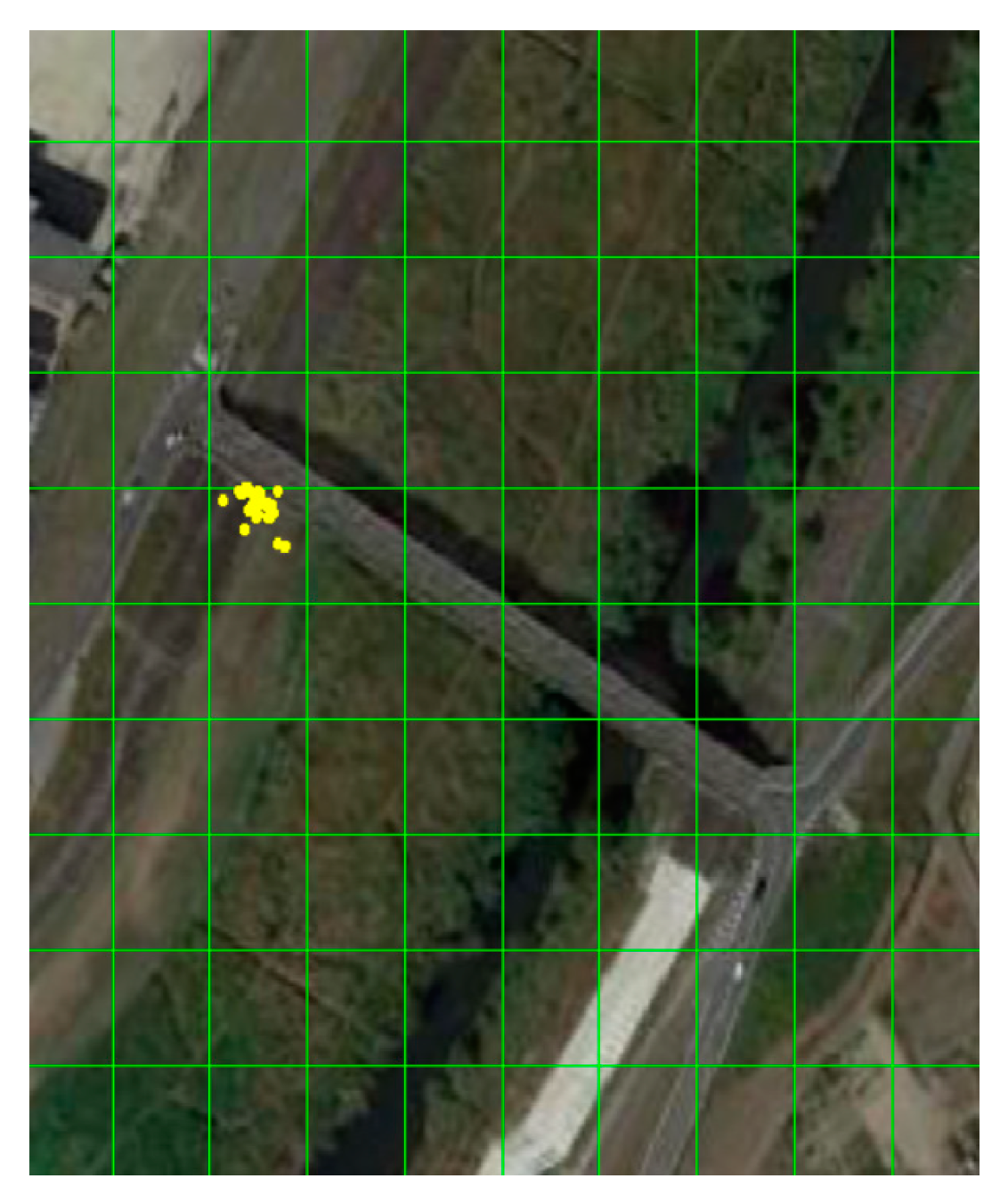
Due to the translation, rotation and deformation of the image, the consistency of feature points cannot be guaranteed for the whole image. If the image is divided into smaller areas, this not only ensures the consistency within the small area, but also reduces the global operation time. Therefore, N×N non-overlapping grid cells are selected to divide the image in this paper, as shown in Figure 1.
If the false match points fall into the correct clustering region, they will be wrongly judged as correct feature matching points. According to the randomness of the false feature points, the grid is taken as the unit, whereas the probability of the false feature match points falling into the correct grid region can be expressed using the following equations:
where is the correct grid region corresponding to the feature match point (see Equation (2)), and is the region outside the correct corresponding grid region (see Equation (3)).
From the probability distribution, the standard deviation of the correct match points of each grid is stable due to consistency, whereas the standard deviation of the false match points fluctuate greatly. Therefore, the false and true match points can be distinguished according to the standard deviation of the feature points’ coordinates, as shown in Figure 4. The mean value and standard deviation of feature points’ coordinates are as follows:
where is the Euclidean distance between the i-th feature point and the center of all feature points within one grid, and n is the number of feature points (see Equations (4) and (5)).
2.1.2. Grid Clustering Statistics
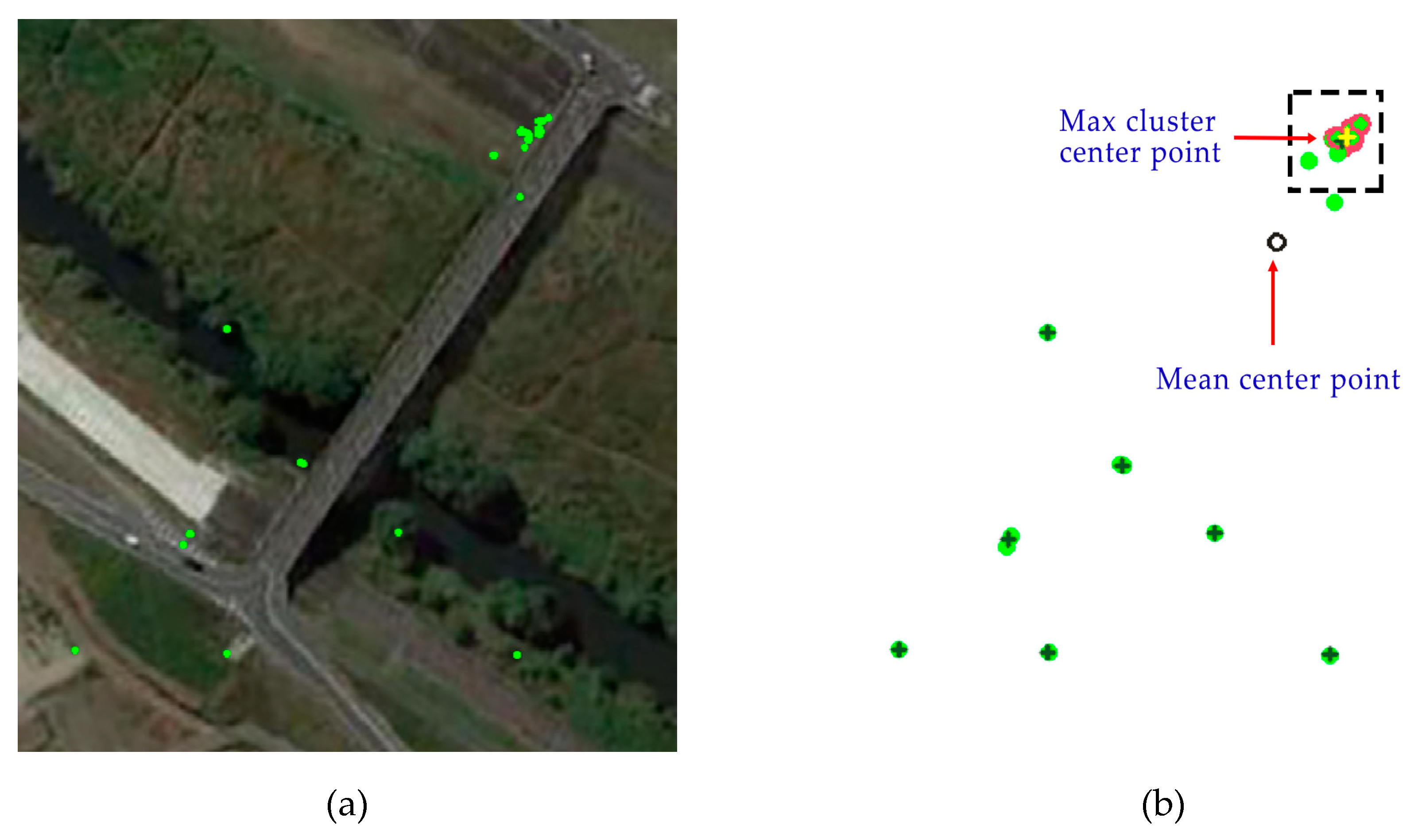
Due to the consistency distribution of the true matches, the position of match points has the effect of aggregation. From the perspective of the standard deviation, the data are stable and easily distinguishable. Even if the number of mismatched points of some grids is greater than that of true matching points, because the mismatched points are random and discrete, it is easy to exclude the mismatched points by identifying mismatched points with large data fluctuations and standard deviations. Therefore, a clustering method is used to obtain the center point of the feature matching, as shown in Figure 5 (the black point is the mean center point, and the blue one is the clustering center point). Meanwhile, the clustering center point is used to analyse the volatility of its standard deviation.
where is the Euclidean distance between the j-th clustering feature point in the c-th cluster and the c-th clustering center, and is the mean of the distance between the c-th clustering center and clustering feature points in the c-th cluster.
To facilitate clustering, mean shift is selected to obtain the clustering center. At the same time, multiples of the grid radius are used as the merger radius of the clustering center to judge whether the clustering centers are merged or not and to calculate the merged new center.
where is the clustering center point, is the clustering center point, is the number of the clustering point, is the number of the clustering points, is the merged new clustering center point, and is the distance from the clustering center point to the clustering center point.
Since there is more than one clustering center in the grid, the proportion of each cluster in the grid is calculated to replace the more time-consuming calculation of standard deviation by counting the number of feature points of each of the clustering categories:
When is greater than the set threshold value T, the cluster has a higher probability density; that is, the cluster can be considered as the correct matching point set.
2.2. Feedback Verification Using Grid Linear Transformation
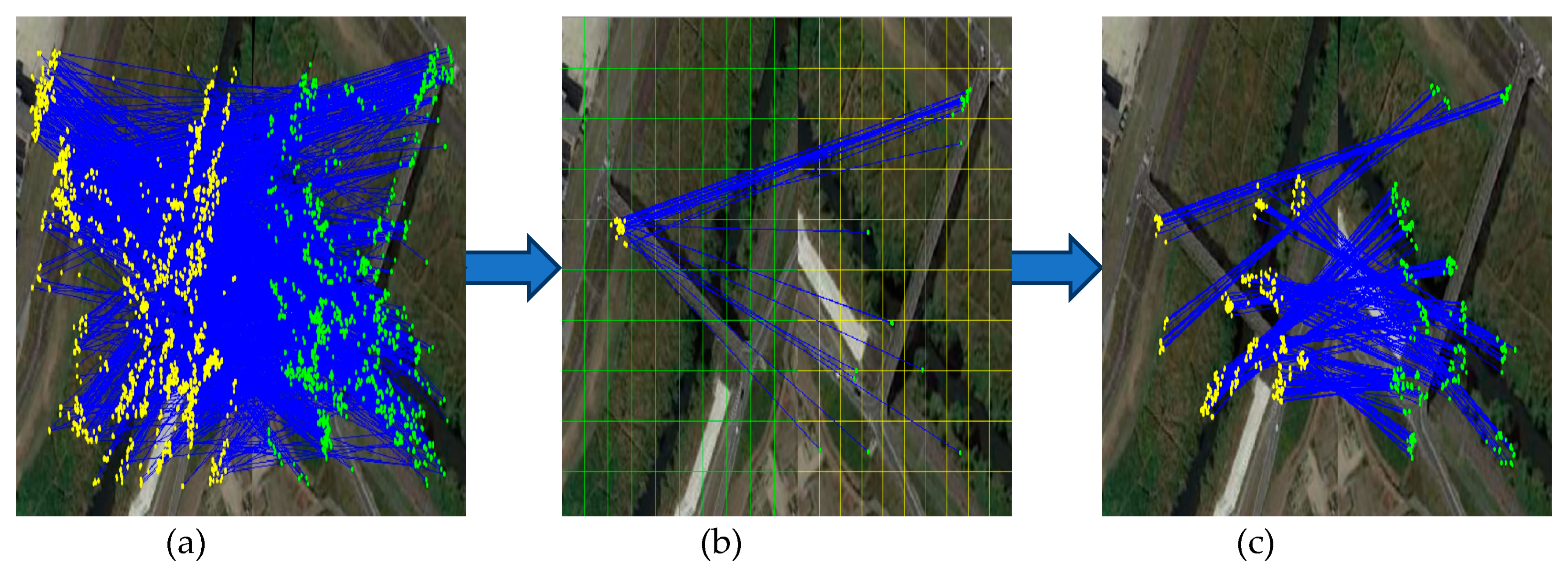
For the general feature matching algorithms, to keep the outlier ratio as low as possible, a simple and effective strategy is to suppress the unstable matches as much as possible; however, such an approach will result in the final match missing a portion of the true matches. This problem also exists in clustering statistics. If the true matches scattered in the grid are at the edge of the correct clustering categories, they are likely to be eliminated. This may be a problem for remote sensing image registration with many relatively obscure textures. At the same time, for remote sensing tasks that rely heavily on feature matching number, such as target recognition, tracking and visual navigation, the loss of true matching will also reduce the final performance, as shown in Figure 6.
To retain as many true matches as possible, this paper presents the grid linear transformation to further extend the feedback verification strategy that performs fine screening between the true match points deleted by mistake and the undeleted false ones in each grid region and its surroundings, potentially extracting the matches with a high rejection rate from the coarse baseline matching with a low false rejection rate (FRR).
Since the feature points in a single grid can be approximated by a simple linear transformation relation, the linear transformation matrix for each grid is calculated; the transformation matrix H-mapping relation between the grid feature points of two images can be expressed as:
Although grid-based clustering results in a large number of true matching feature points being eliminated by mistake, and the false ones also being removed as much as possible, it is more reliable for constructing the correct linear transformation formulas.
The corresponding transformation matrix is calculated by selecting the feature points after grid-based clustering, and since the solution of this model can be regarded as the solution of overdetermined equations, the solution of the equation with the smallest deviation as parameter by the least squares method, where the residual sum of squares function S is:
Above, X and Y are the sets of matching feature points corresponding to the two images.
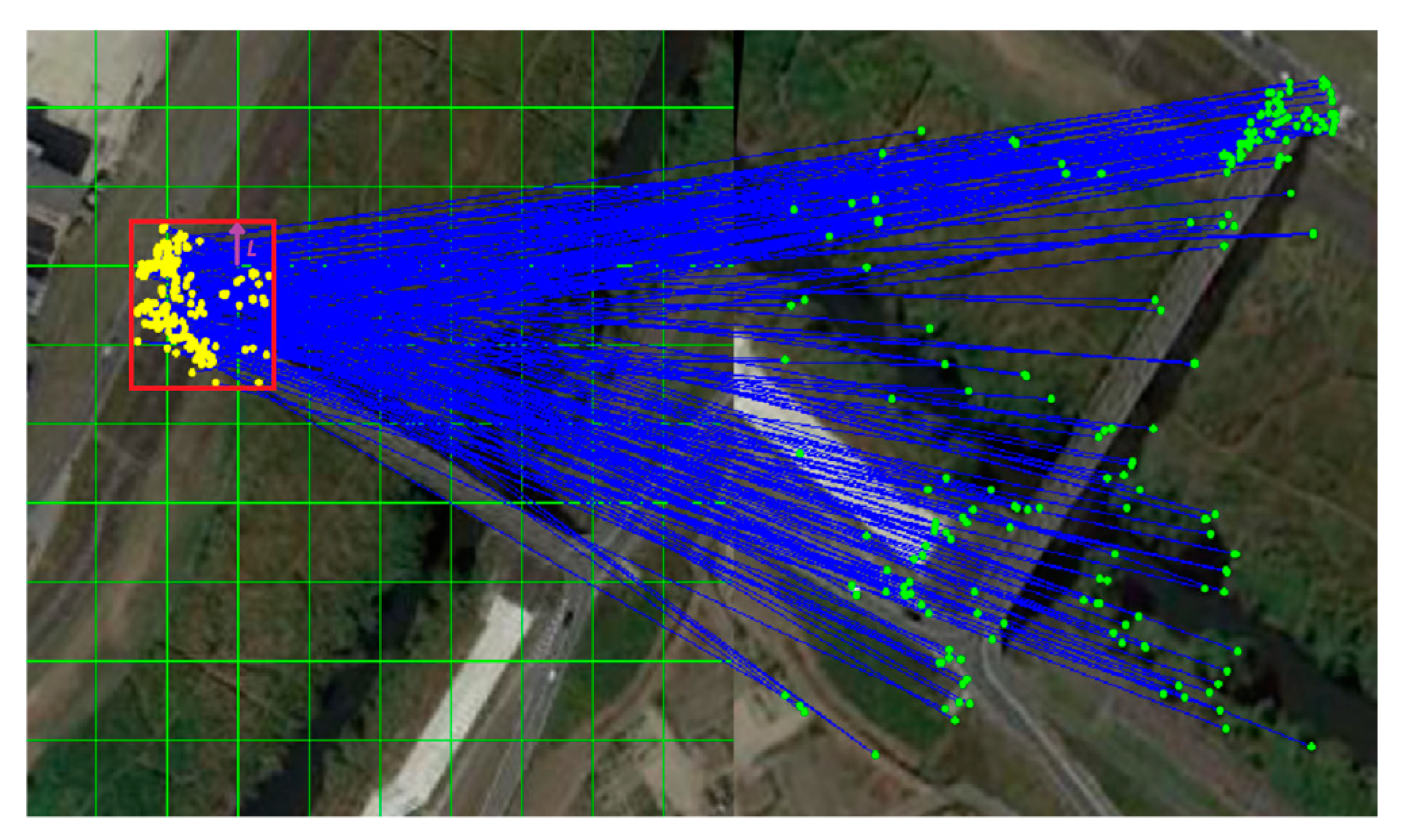
Since grid division may divide the true matches of a cluster into different grids, to ensure that as many true match points are obtained as possible, the grid is extended by an appropriate distance L during feedback verification, as shown in Figure 7.
The matching distance error of each feature point in the expanded grid is calculated by a linear transformation formula. Additionally, a distance error threshold value τ is added for verification, and the matching distance error function can be expressed as:
where and are the coordinates of the match feature points corresponding to the two images, and is the corresponding coordinate of after conversion.
The feature point is a true match if . Because feedback verification is processed by using linear transform, the size of τ is used to tolerate the influence of local nonlinear transform. In most cases, feedback validation enlarging half of the grid is sufficient.
Therefore, the experiment generally set L = half of the grid width and τ = 10 pixels for verification and to obtain satisfactory results, as shown in Figure 8. In Algorithm 1, FUGC process is summarized.
| Algorithm 1: Fugc Algorithm |
| Input: One pair of images |
| Output: Inliers set |
| 1: Detect ORB feature points |
| 2: Use Brute-Force for initial matching point |
| 3: Divide one images by G grids |
| 4: for i = 1 to G do |
| 5: Compute the clustering centers of corresponding image feature points in the grid; |
| 6: repeat: |
| 7: if then |
| 8: |
| 9: end if |
| 10: until: traverse all clustering centers |
| 11: repeat: |
| 12: when , compute the transformation matrix using the corresponding matching points of |
| 13: Expand the grid size and validate |
| if then |
| 14: represents true matching points |
| 15: end if |
3. Results and Discussion
To verify the performance of the FUGC algorithm, the following aspects of the algorithm’s performance is evaluated: precision, recall rate, and time consumption. FUGC is compared to powerful matchers such as RANSAC, VCF, GSM and UGC. During the entire experiment, the parameters of the algorithm remain consistent. The experiments are performed on a laptop with a 2.4 GHz i7 Intel Core Central Processing Unit (CPU) and 8 GB of Random Access Memory (RAM), using the open source toolkit OpenCV 3.0.
3.1. Datasets and Settings
To evaluate the FUGC algorithm comprehensively, experiments are carried out on four remote sensing image datasets. We manually cut, scale and rotate the images to obtain the corresponding images to be matched (Supplementary Materials).
- (1)
- Dataset for Object Detection in Aerial Images (DOTA) is a large-scale dataset for object detection in aerial Images. Altogether, there are 2806 remote sensing images with the size of approximately 4000 × 4000; there are 188,282 instances divided into 15 categories, including airplanes, playgrounds, overpasses, farmland and others.
- (2)
- National Oceanic and Atmospheric Administration (NOAA) is a dataset of digital coastline; it includes seabed data, elevation, image, land cover and socio-economic information. There are 245 images in this test set, and the data type is infrared.
- (3)
- Dataset for Object Detection in Remote Sensing Images (RSOD) is a dataset for object detection in aerial images, including four types of targets: aircraft, playgrounds, flyovers and oil drums. The numbers of targets are 446, 189, 176 and 165, respectively.
- (4)
- University of Chinese Academy of Sciences (UCAS) is a dataset for object detection in aerial images, containing only two types of targets: vehicles and aircraft. There are 1000 images of aircraft and 510 images of vehicles.
3.2. Experimental Results
To compare the algorithms’ performance, the number of feature points is fixed to 3000, and the OpenCV’s ORB features are used uniformly. Because the FUGC algorithm places a particular emphasis on the screening of matching feature points and eliminating false matches, and does not depend on any particular feature, the feature points collection is performed during the initial matching using the greedy matching brute force algorithm; the brute force algorithm can be GPU-accelerated to improve the matching speed. The quality of matching is represented by the precision, recall and balanced F1-score, where the precision is the ratio of the number of the final true matches to the total number of final matches and the recall is the ratio of the number of final true matches to the total number of initial true matches. F1 is the harmonic average of the precision and recall. Before the experiment, the dimensions of the test images are standardized to 640×480. According to the previous discussion of the UGC method, when the grid is set to 18×18, the accuracy and time of the method can be balanced to the maximum extent possible; R is 0.75 times the grid width, L is 0.5 times the grid width, T is 0.5 times the total number of grid feature points, and τ is 10 pixels.
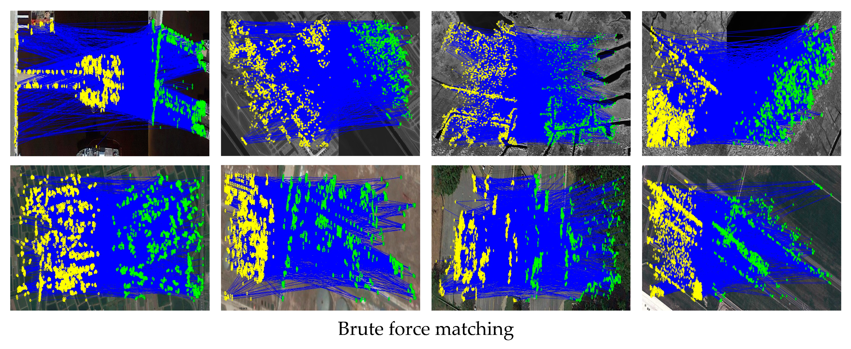
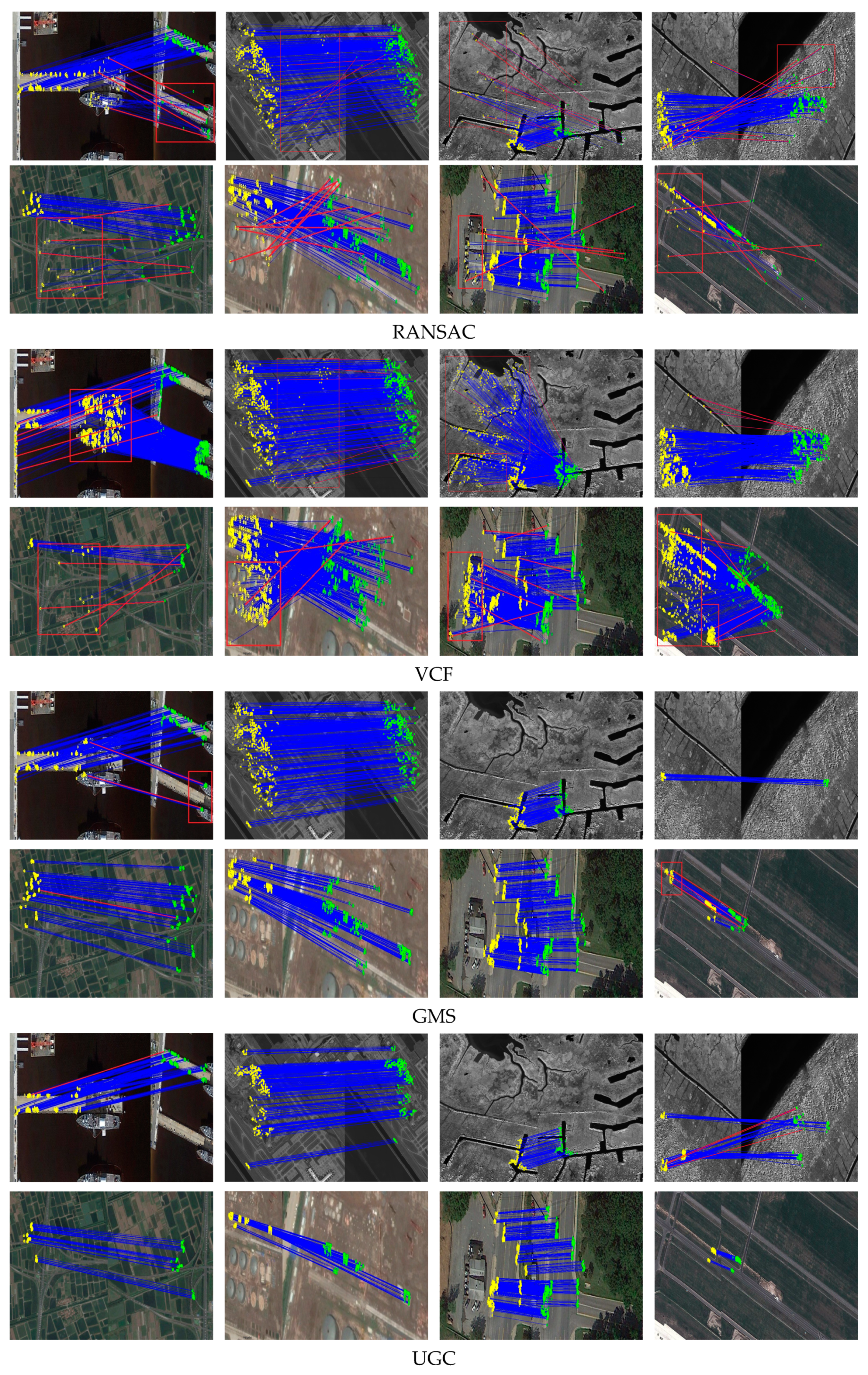
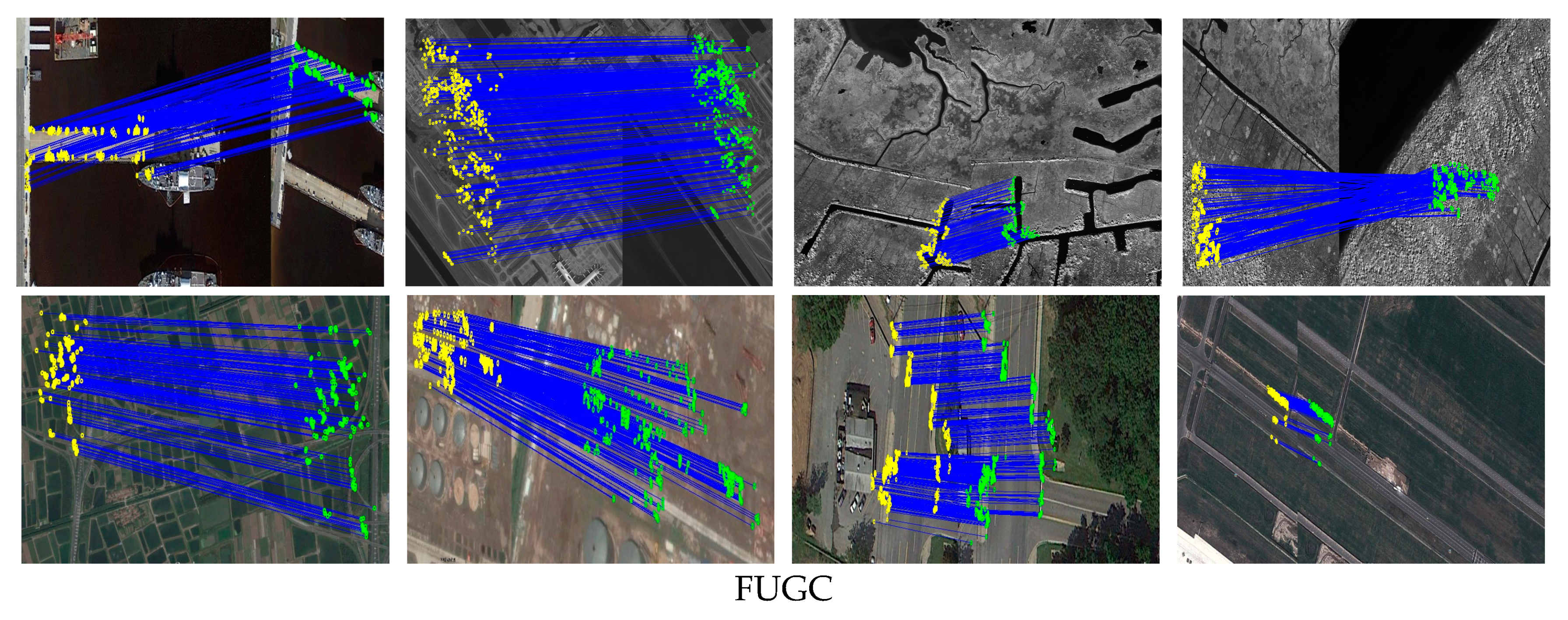
Some representative image matching effects selected from the testing dataset are displayed in Figure 9. These eight images correspond to four datasets—DOTA, NOAA, RSOD and UCAS—where each dataset contains two typical image pairs. It is a challenging task to establish a reliable correspondence between these images due to problems such as the small overlap involved, severe noise, large change in viewpoint transformation, or low resolution. The matching results of the FUGC algorithm and several other state-of-the-art feature matching methods, including RANSAC, VCF, GSM and UGC, are shown in Figure 9. The beginning and end of each blue line in Figure 9 correspond to the positions of the corresponding feature points in the two images, and the red line and red box are partial false matches. Since the simple and fast brute force matching strategy is used instead of some complex strategies to construct the assumed correspondence, at the same time, the average number of matches in the initial hypothesis set is set to 3000; to make the dataset challenging, the true matching percentage in the initial hypothesis is set to be relatively low.
According to the matching results in Figure 9, when the initial hypothesis set does not contain many outliers, RANSAC can produce satisfactory results. However, its performance decreases rapidly with an increasing number of outliers, e.g., in an affine dataset. The performance of VCF is not very satisfactory: although it has a high recall rate, it lacks robustness at higher outlier counts; in particular, it fails completely on image pairs with a very low percentage of true matches. GMS obtains very low matching errors, but a large number of true matching pairs are lost. UGC has fewer mismatches than GMS but it also has more missing correct matches. In contrast, the FUGC method can not only eliminate a large number of false matches from the assumed correspondence of the image pairs, but also retain as many true matches as possible. This observation shows that the FUGC method can address various matching problems of remote sensing images, including remote sensing data and image transformations of various types.
Next, a quantitative comparison of FUGC and the aforementioned state-of-the-art feature matching methods is performed. All the comparison methods were based on publicly available core C++ code and we adjusted the parameters to ensure the best settings. All code was implemented without special optimizations, such as parallel computation or multithreading.
Recall and precision rate are key indicators of image registration. Usually, recall and precision are expressed by the following formula:
where correct_matches is the number of correct matches in the filtered results, correspondences is the number of correct matches in the initial assumed matching set (after brute force matching), and false_matches is the number of false matches in the filtered results.
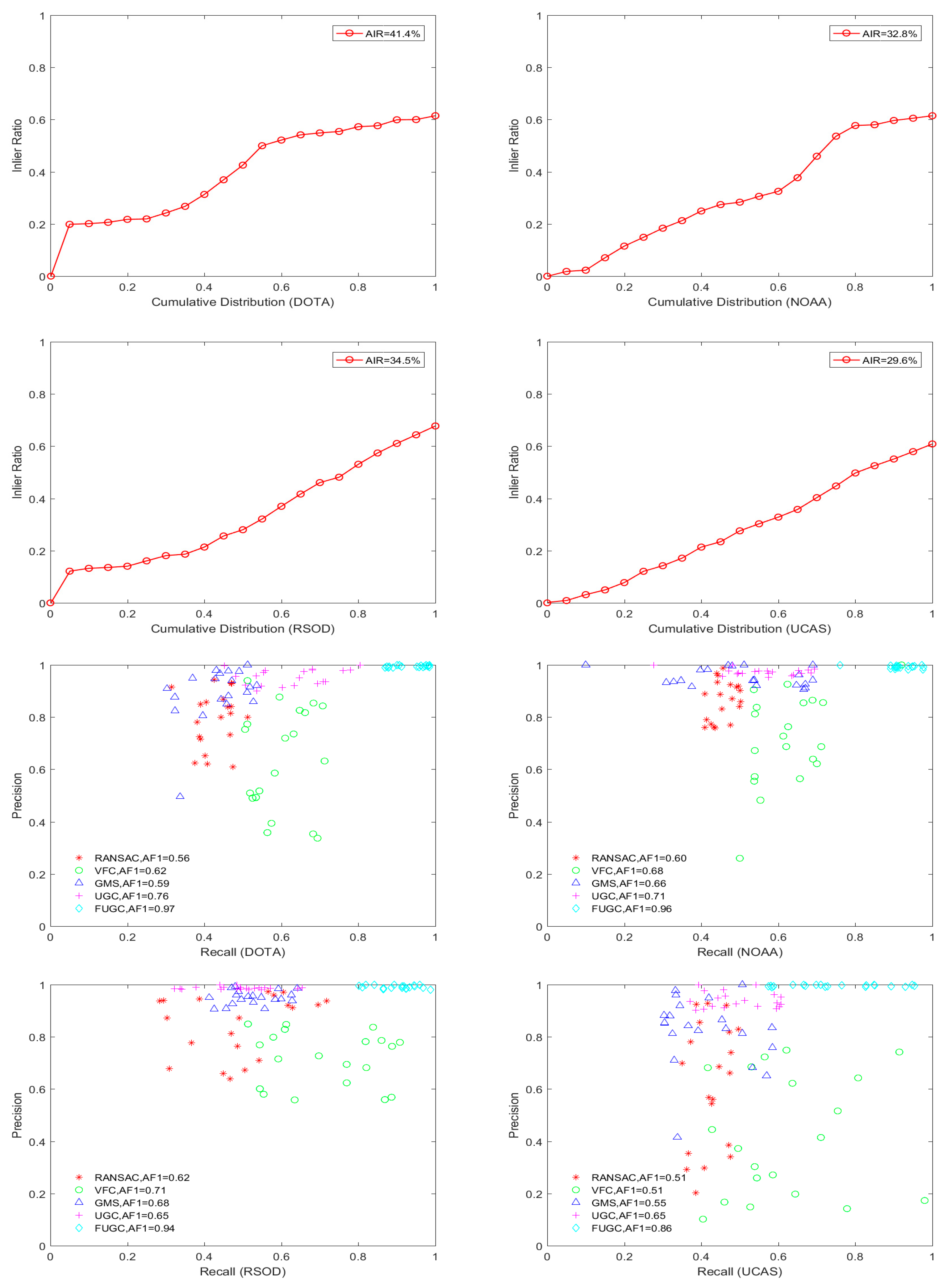
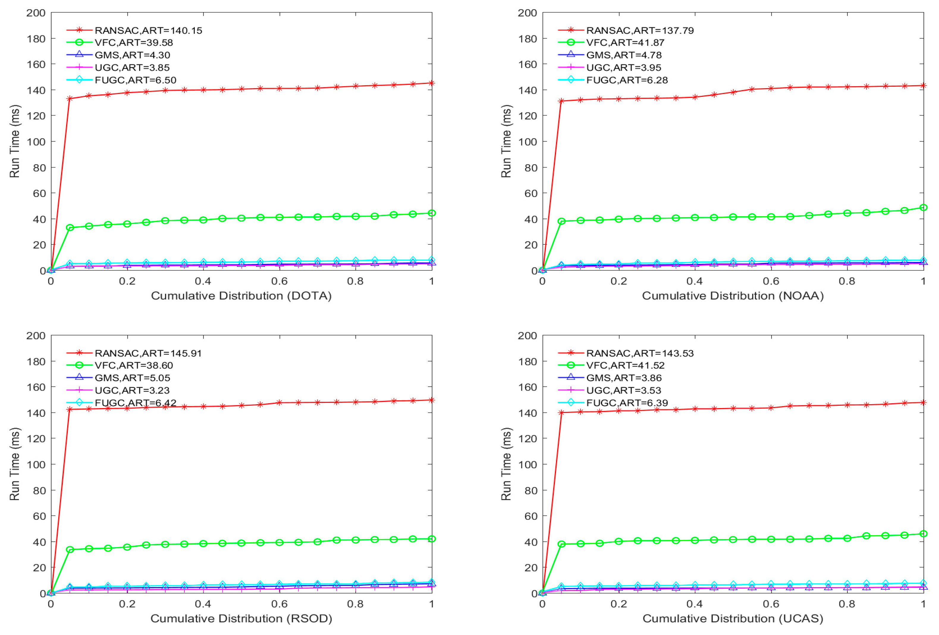
The initial inlier ratio, precision recall rate and the running time of various methods are shown in Figure 10. The initial inlier ratio is the precision of 3000 feature matches after brute force matching. The initial inlier ratio in the UCAS dataset is very low, whereas the average inlier ratio (AIR) is only approximately 29.7%. The third and fourth line of Figure 10 shows the precision and recall rate of each algorithm, in addition to the respective calculated average F1 scores. In the figure, the precision and recall rate are selected through equal intervals after sorting all the precision and recall rates. It is observed that both the precision and recall rate of RANSAC are poor, especially in the case of a low inlier ratio, such as that of the UCAS dataset, where it performs much worse. The recall rate of VFC is relatively higher, but the precision is not good, mainly because this algorithm results in the retention of a large number of false matches in order to retain more true matches. GMS and UGC have higher precision but a lower recall rate. Because their strategy is to strictly reject false matches, a large number of true matches are also removed. In comparison, the FUGC method obviously has the best matching performance on all datasets, with the precision and recall rate of most image pairs being close to one. In addition, on all four datasets, the precision, recall rate and the average F1 (AF1) score of FUGC are all higher than those of other algorithms, indicating the effectiveness of the feedback verification strategy of FUGC.
In the last two lines of Figure 10, the running times of the five algorithms are shown. The running time does not include the feature point detection or the brute force matching. The average running times of the RANSAC and VFC algorithms on the four datasets are significantly greater than 10 ms, whereas the average running times of the GMS, UGC and FUGC algorithms are within 10 ms. Although FUGC is slower than GMS and UGC, the longest average running time is only 7 ms and does not violate the requirements of real-time applications. Therefore, the FUGC method can significantly improve the matching precision and recall rate under certain real-time requirements to better meet the requirements of remote sensing for matching precision.
4. Conclusions
FUGC is a type of false matching elimination method for feature matching of remote sensing imagery. It is based on the principle of local neighborhood consistency; the method filters the true and false match pairs using feedback verification of the local clustering analysis and a linear transformation. This idea makes the algorithm’s theory much simpler, significantly improves the matching precision and the recall rate, and ensures the algorithm’s real-time performance. The results show that the FUGC algorithm incorporating feedback verification overcame the problem that the UGC and GSM algorithm lost a large number of correct matching points in previous studies, and produced the most accurate results. In addition, the feedback verification threshold of the FUGC algorithm will affect the matching performance, which will be an important research direction for improving the robustness of matching.
Supplementary Materials
The DOTA data set are available online at http://captain.whu.edu.cn/DOTAweb/. The NOAA data set are available online at https://www.ngdc.noaa.gov/mgg/shorelines/. The RSOD data set are available online at http://download.intergraph.com/downloads/erdas-imagine-2013-2014-example-data. The UCAS data set are available online at http://download.intergraph.com/downloads/erdas-imagine-2013-2014-example-data. The FUGC code is available online at https://github.com/DoctorZheng/F-UGC.
Author Contributions
Z.Z., H.Z., Y.M., F.F., J.J., B.X., M.L. and S.C. together conceptualized the study and designed the methodology and experiments. Z.Z. performed the experiments, and prepared the first draft of the manuscript. B.X. and M.L. participated in the research data collection, analysis and interpretation. F.F. reviewed, expanded and edited the manuscript. H.Z. and Y.M. guided the experiments and the statistical analysis, J.J. and S.C. supplied help with the experiments and paper revision.
Funding
This research was partially supported by the National Natural Science Foundation of China under Grants 61605146, 61275098, 61503288, the Wuhan Railway Vocational College Foundation of China, No. Y2018015, and the Fundamental Research Funds for the Central Universities, No.31541411210.
Conflicts of Interest
The authors declare no conflicts of interest.
References
- Zitova, B.; Flusser, J. Image Registration Methods: A Survey. Image Vis. Comput. 2003, 21, 977–1000. [Google Scholar] [CrossRef]
- Zheng, Z.H.; Ma, Y.; Zheng, H.; Gu, Y.; Lin, M.Y. Industrial part localization and grasping using a robotic arm guided by 2D monocular vision. Ind. Robot. J. 2018, 45, 794–804. [Google Scholar] [CrossRef]
- Ma, J.; Jiang, J.; Liu, C.; Li, Y. Feature Guided Gaussian Mixture Model with Semi-Supervised EM and Local Geometric Constraint for Retinal Image Registration. Inf. Sci. 2017, 417, 128–142. [Google Scholar] [CrossRef]
- Guo, Y.; Bennamoun, M.; Sohel, F.; Lu, M.; Wan, J.W. 3D Object Recognition in Cluttered Scenes with Local Surface Features: A Survey. IEEE Trans. Pattern Anal. Mach. Intell. 2014, 36, 2270–2287. [Google Scholar]
- Ma, J.Y.; Zhou, H.B.; Zhao, J.; Gao, Y.; Jiang, J.; Tian, J. Robust Feature Matching for Remote Sensing Image Registration via Locally Linear Transforming. IEEE Trans. Geosci. Remote Sens. 2015, 53, 6469–6481. [Google Scholar] [CrossRef]
- Ma, J.; Jiang, X.; Jiang, J.; Zhao, J.; Guo, X. LMR: Learning A Two-class Classifier for Mismatch Removal. IEEE Trans. Image Process. 2019, 1–15. [Google Scholar] [CrossRef] [PubMed]
- Lowe, D. Distinctive image features from scale-invariant keypoints. Int. J. Comput. Vis. 2004, 60, 91–110. [Google Scholar] [CrossRef]
- Rublee, E.; Rabaud, V.; Konolige, K.; Bradski, G. Orb: An efficient alternative to sift or surf. In Proceedings of the International Conference on Computer Vision, Barcelona, Spain, 6–13 November 2011; pp. 2564–2571. [Google Scholar]
- Bay, H.; Tuytelaars, T.; Gool, L.V. SURF: Speeded up robust features. In Proceedings of the European Conference on Computer Vision, Graz, Austria, 7–13 May 2006; pp. 404–417. [Google Scholar]
- Ma, J.; Wu, J.; Zhao, J.; Jiang, J.; Zhou, H.; Sheng, Q.Z. Nonrigid Point Set Registration with Robust Transformation Learning under Manifold Regularization. IEEE Trans. Neural Netw. Learn. Syst. 2018, 1–14. [Google Scholar] [CrossRef] [PubMed]
- Ma, J.; Zhao, J.; Tian, J.; Bai, X.; Tu, Z. Regularized Vector Field Learning with Sparse Approximation for Mismatch Removal. Pattern Recognit. 2013, 46, 3519–3532. [Google Scholar] [CrossRef]
- Belongie, S.; Mori, G.; Malik, J. Matching with Shape Contexts. In Statistics and Analysis of Shapes; Birkhäuser: Boston, MA, USA, 2006; pp. 81–105. [Google Scholar]
- Zaharescu, A.; Boyer, E.; Varanasi, K.; Horaud, R. Surface feature detection and description with applications to mesh matching. In Proceedings of the IEEE Conference on Computer Vision and Pattern Recognition, Miami, FL, USA, 20–25 June 2009; pp. 373–380. [Google Scholar]
- Torr, P.H.S.; Zisserman, A. MLESAC: A new robust estimator with application to estimating image geometry. Comput. Vis. Image Underst. 2000, 78, 138–156. [Google Scholar] [CrossRef]
- Chum, O.; Matas, J.; Obdrzalek, S. Enhancing ransac by generalized model optimization. In Proceedings of the Asian Conference on Computer Vision, Jeju, Korea, 27–30 January 2004. [Google Scholar]
- Chum, O.; Matas, J. Matching with PROSAC—Progressive sample consensus. In Proceedings of the IEEE Conference on Computer Vision and Pattern Recognition, San Diego, CA, USA, 20–25 June 2005; pp. 220–226. [Google Scholar]
- Besl, P.J.; McKay, N.D. A Method for Registration of 3-D Shapes. In Proceedings of the SPIE—The International Society for Optical Engineering, Orlando, FL, USA, 22–24 April 1992; Volume 14, pp. 239–256. [Google Scholar]
- Chui, H.; Rangarajan, A. A new point matching algorithm for non-rigid registration. Comput. Vis. Image Underst. 2003, 89, 114–141. [Google Scholar] [CrossRef]
- Ma, J.Y.; Qiu, W.C.; Zhao, J.; Tu, Z. Robust l2e estimation of transformation for non-rigid registration. IEEE Trans. Signal Process. 2015, 63, 1115–1129. [Google Scholar] [CrossRef]
- Bing, J.; Vemuri, B.C. A Robust Algorithm for Point Set Registration Using Mixture of Gaussians. In Proceedings of the IEEE International Conference on Computer Vision, Beijing, China, 17–21 Octomber 2005; pp. 1–13. [Google Scholar]
- Myronenko, A.; Song, X. Point set registration: Coherent point drift. IEEE Trans. Pattern Anal. Mach. Intell. 2010, 32, 2262–2275. [Google Scholar] [CrossRef] [PubMed]
- Ma, J.; Zhao, J.; Jiang, J.; Zhou, H.; Guo, X. Locality Preserving Matching. Int. J. Comput. Vis. 2019, 127, 512–531. [Google Scholar] [CrossRef]
- Ma, J.Y.; Jiang, J.J.; Zhou, H.B.; Zhao, J.; Guo, X.J. Guided Locality Preserving Feature Matching for Remote Sensing Image Registration. IEEE Trans. Geosci. Remote Sens. 2018, 56, 4435–4447. [Google Scholar] [CrossRef]
- Fischler, M.A.; Bolles, R.C. Random Sample Consensus: A Paradigm for Model Fitting with Applications to Image Analysis and Automated Cartography. In Readings in Computer Vision; Morgan Kaufmann: Burlington, MA, USA, 1987; pp. 726–740. [Google Scholar]
- Ma, J.Y.; Zhao, J.; Tian, J.T.; Yuille, A.L.; Tu, Z. Robust point matching via vector field consensus. IEEE Trans. Image Process. 2014, 23, 1706–1721. [Google Scholar]
- Bian, J.W.; Lin, W.Y.; Matsushita, Y.; Yeung, S.K.; Nguyen, T.D. GMS: Grid-based Motion Statistics for Fast, Ultra-Robust Feature Correspondence. In Proceedings of the IEEE Conference on Computer Vision and Pattern Recognition (CVPR), Honolulu, HI, USA, 21–26 July 2017; pp. 4181–4190. [Google Scholar]
- Zheng, Z.H.; Ma, Y.; Zheng, H.; Ju, J.P.; Lin, M.Y. UGC: Real-Time, Ultra-Robust Feature Correspondence via Unilateral Grid-Based Clustering. IEEE Access 2018, 6, 55501–55508. [Google Scholar] [CrossRef]
Figure 1.
The image is divided into 10 × 10 non-overlapping grid cells, where the feature points in a grid cell are marked in yellow.
Figure 1.
The image is divided into 10 × 10 non-overlapping grid cells, where the feature points in a grid cell are marked in yellow.

Figure 2.
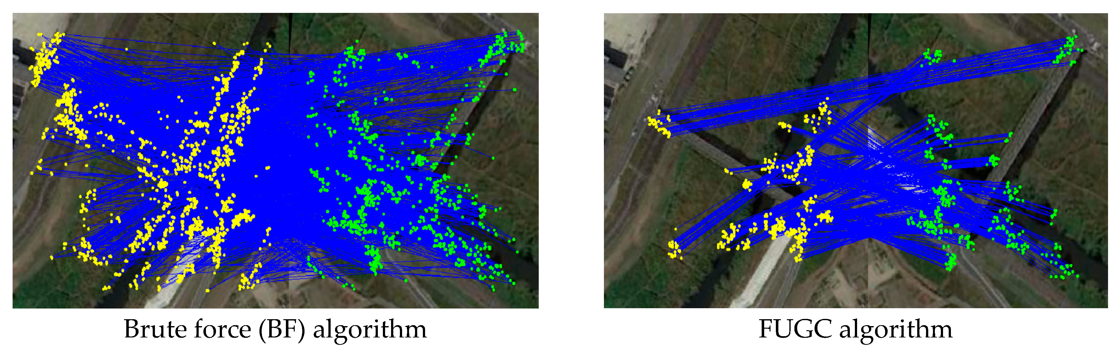
The left figure is the matching result of the brute force algorithm, and the right one is the matching result of the feedback unilateral grid-based clustering (FUGC) algorithm. The brute force (BF) algorithm relies on comparing each feature point with all possible candidate feature points belonging to the corresponding search area by computing the distance between feature points. The yellow points and green points represent feature points. The blue lines represent all matches. Clearly, the FUGC algorithm not only ensures the accuracy of matching but also retains as many correct matches as possible.
Figure 2.
The left figure is the matching result of the brute force algorithm, and the right one is the matching result of the feedback unilateral grid-based clustering (FUGC) algorithm. The brute force (BF) algorithm relies on comparing each feature point with all possible candidate feature points belonging to the corresponding search area by computing the distance between feature points. The yellow points and green points represent feature points. The blue lines represent all matches. Clearly, the FUGC algorithm not only ensures the accuracy of matching but also retains as many correct matches as possible.

Figure 3.
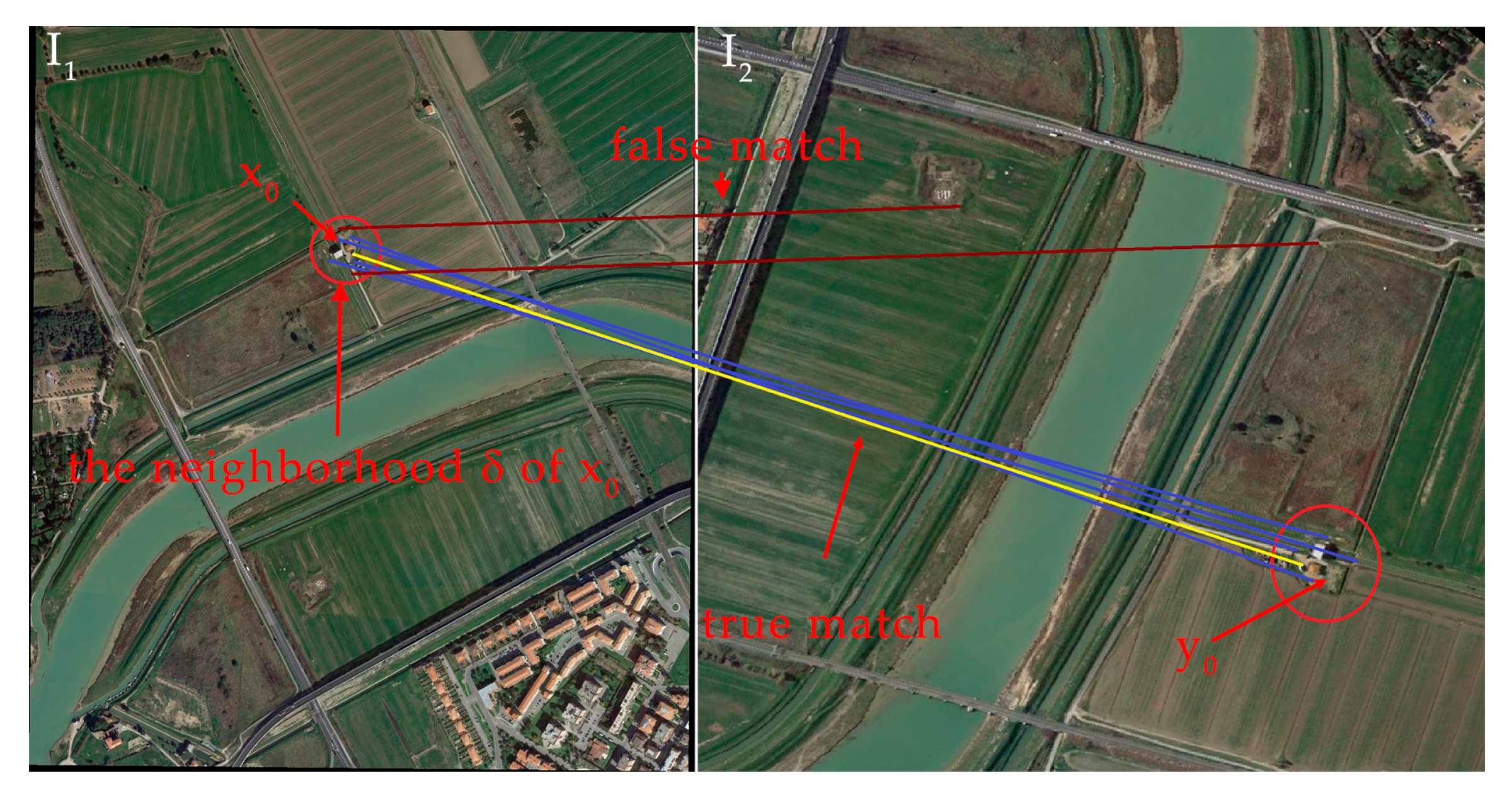
In the neighbourhood of a matching point, the true matching points are consistent, whereas the false ones are not. is the feature point of image I1 and is the corresponding feature point of image I2.
Figure 3.
In the neighbourhood of a matching point, the true matching points are consistent, whereas the false ones are not. is the feature point of image I1 and is the corresponding feature point of image I2.

Figure 4.
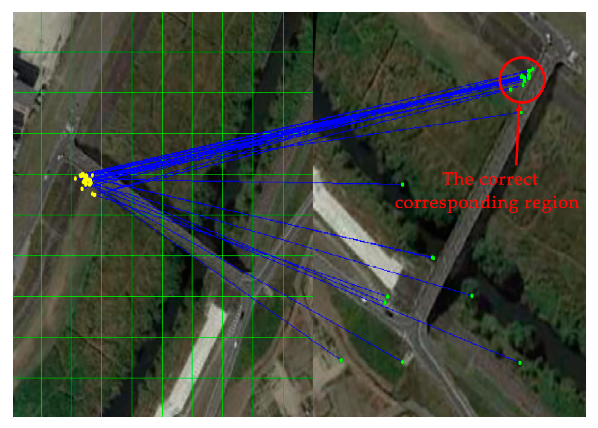
Feature points in a grid of the left image correspond to the match points of the right image. The red circle in the right image shows the true match points, which is characterized by aggregation.
Figure 4.
Feature points in a grid of the left image correspond to the match points of the right image. The red circle in the right image shows the true match points, which is characterized by aggregation.

Figure 5.
(a) One grid field from the initial match figure with detected feature points (represented as green dots). (b) Clustering of the same feature points, where the green circle and red circle represent the match points, the black cross represents the clustering center points, the yellow cross represents the maximum clustering center points, the black circle represents the mean center points, and the dotted box represents the maximum clustering area.

Figure 6.
Schematic diagram of the UGC algorithm matching strategy: although false matches are completely rejected, it is clear that a large number of true matches are also rejected. (a) Initial matching results, (b) matching results after a grid clustering, and (c) UGC final matching results.
Figure 6.
Schematic diagram of the UGC algorithm matching strategy: although false matches are completely rejected, it is clear that a large number of true matches are also rejected. (a) Initial matching results, (b) matching results after a grid clustering, and (c) UGC final matching results.

Figure 7.
Schematic diagram of grid expansion.

Figure 8.
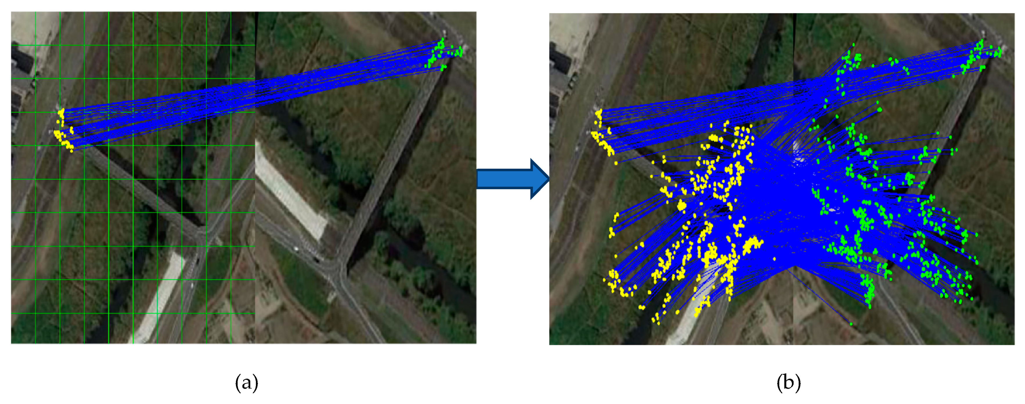
Feedback verification results of FUGC matching. (a) Feedback verification results after grid expansion. (b) Final matching result of the FUGC method.
Figure 8.
Feedback verification results of FUGC matching. (a) Feedback verification results after grid expansion. (b) Final matching result of the FUGC method.

Figure 9.
Results for several typical image pairs of the four testing datasets, namely, DOTA, NOAA, RSOD and UCAS, obtained using the RANSAC, VCF, GMS, UGC and FUGC algorithms. The red boxes and red lines on the maps are examples of incorrectly established matches. It is clear that FUGC performs better in both matching precision and the number of final matches.


Figure 10.
Quantitative comparison of the RANSAC, VCF, GSM, UGC and FUGC algorithms on the four testing datasets, namely, DOTA, NOAA, RSOD and UCAS. AIR = average inlier ratio, AF1 = average F1 score and ART = average running time.
Figure 10.
Quantitative comparison of the RANSAC, VCF, GSM, UGC and FUGC algorithms on the four testing datasets, namely, DOTA, NOAA, RSOD and UCAS. AIR = average inlier ratio, AF1 = average F1 score and ART = average running time.


© 2019 by the authors. Licensee MDPI, Basel, Switzerland. This article is an open access article distributed under the terms and conditions of the Creative Commons Attribution (CC BY) license (http://creativecommons.org/licenses/by/4.0/).
Share and Cite
MDPI and ACS Style
Zheng, Z.; Zheng, H.; Ma, Y.; Fan, F.; Ju, J.; Xu, B.; Lin, M.; Cheng, S. Feedback Unilateral Grid-Based Clustering Feature Matching for Remote Sensing Image Registration. Remote Sens. 2019, 11, 1418. https://doi.org/10.3390/rs11121418
AMA Style
Zheng Z, Zheng H, Ma Y, Fan F, Ju J, Xu B, Lin M, Cheng S. Feedback Unilateral Grid-Based Clustering Feature Matching for Remote Sensing Image Registration. Remote Sensing. 2019; 11(12):1418. https://doi.org/10.3390/rs11121418
Chicago/Turabian StyleZheng, Zhaohui, Hong Zheng, Yong Ma, Fan Fan, Jianping Ju, Bichao Xu, Mingyu Lin, and Shuilin Cheng. 2019. "Feedback Unilateral Grid-Based Clustering Feature Matching for Remote Sensing Image Registration" Remote Sensing 11, no. 12: 1418. https://doi.org/10.3390/rs11121418
Note that from the first issue of 2016, this journal uses article numbers instead of page numbers. See further details here.