A New Single-Band Pixel-by-Pixel Atmospheric Correction Method to Improve the Accuracy in Remote Sensing Estimates of LST. Application to Landsat 7-ETM+


Abstract
:
1. Introduction
2. Materials and Methods
2.1. Atmospheric Correction in the TIR Domain
2.2. SBAC Method
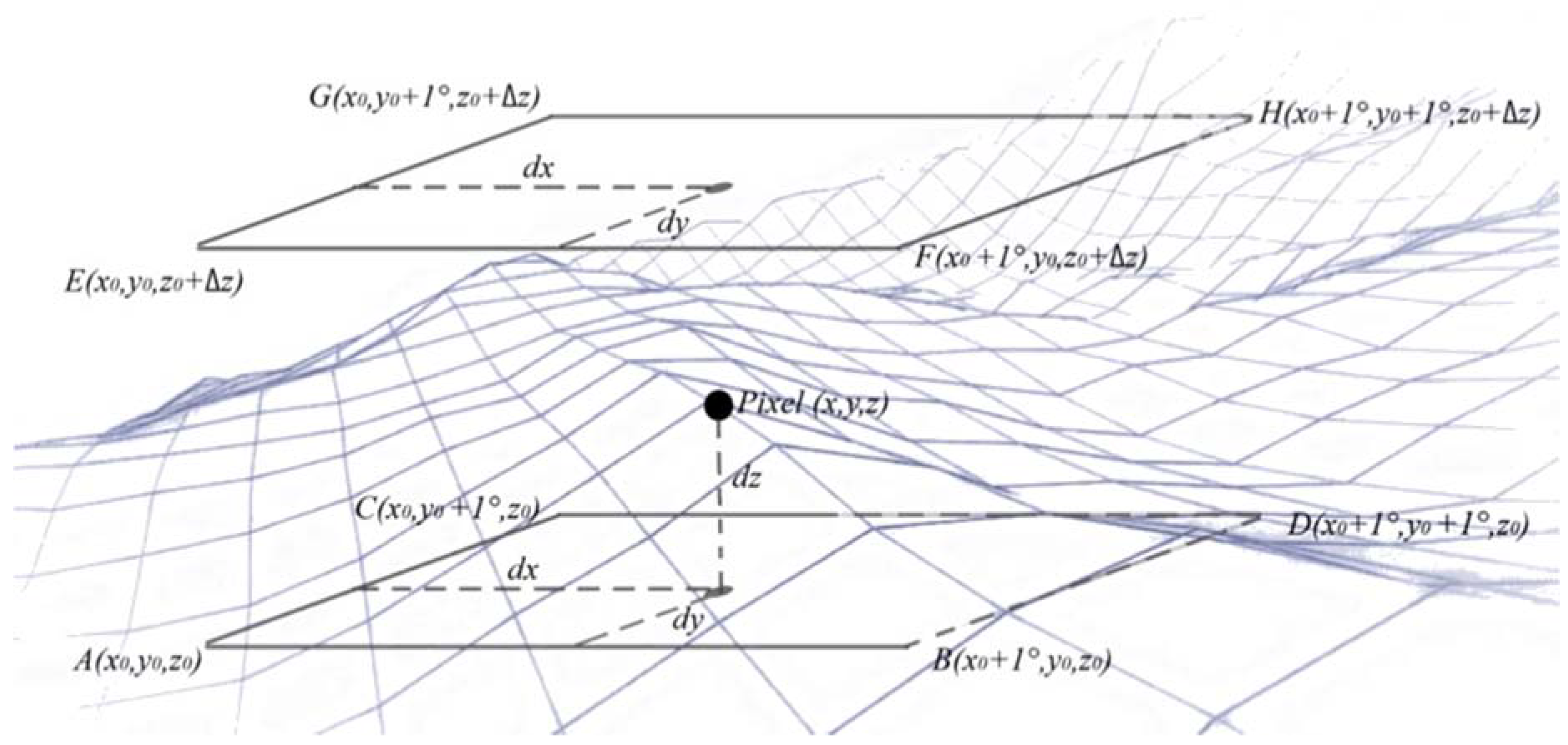
- (a)
- When the prescribed z0 value is located between two NCEP layers, the corresponding air temperature and humidity are obtained by linear interpolation from the original NCEP levels, all the upper NCEP layers remaining unchanged and all the layers below the prescribed altitude z0 being ignored.
- (b)
- When the prescribed altitude z0 is below the lowest level of the NCEP profile, we take the NCEP altitude as the lowest z0 in the 1° × 1° node and do not consider any z0 value below it.
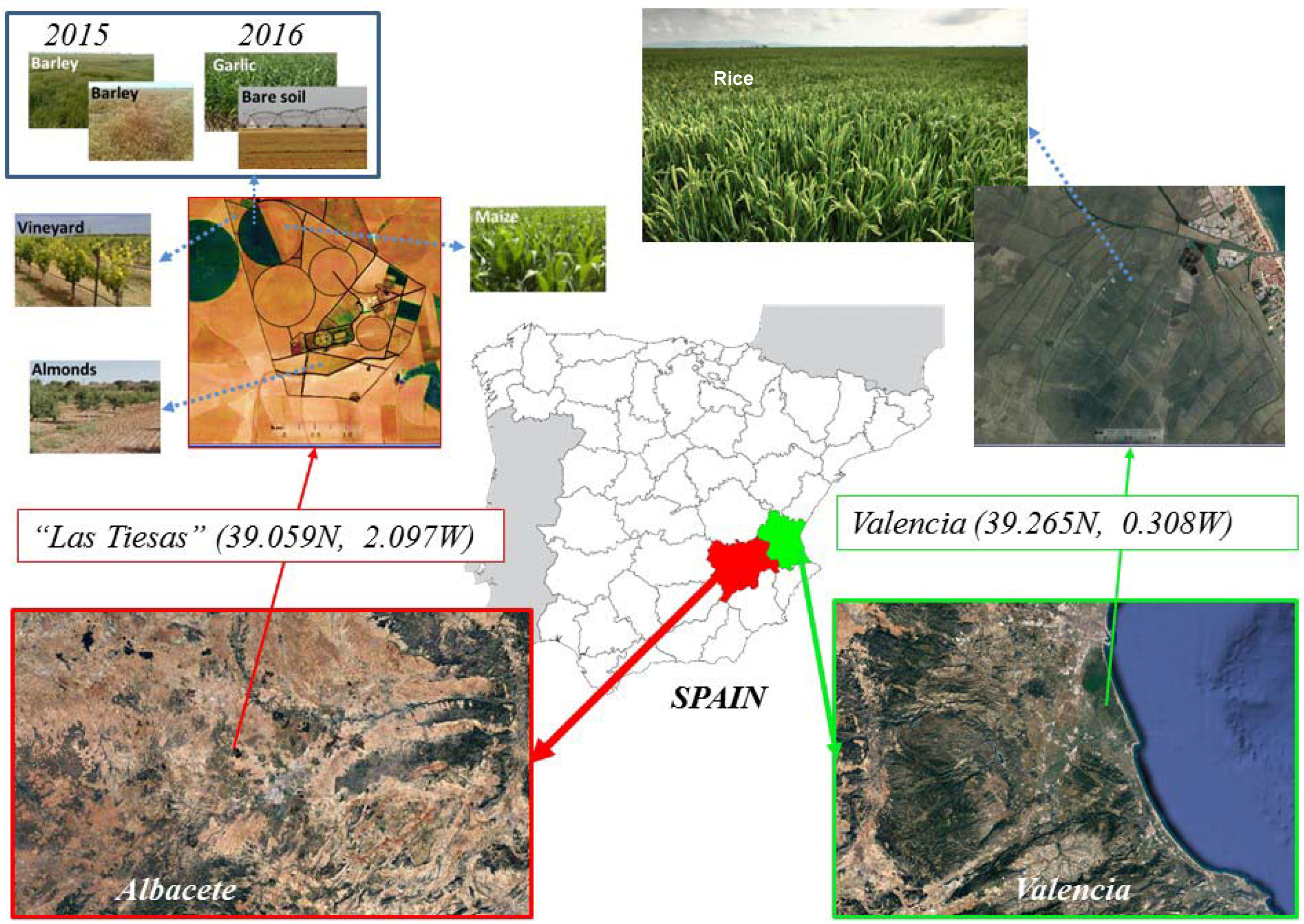
2.3. Study Sites and Ground Measurements
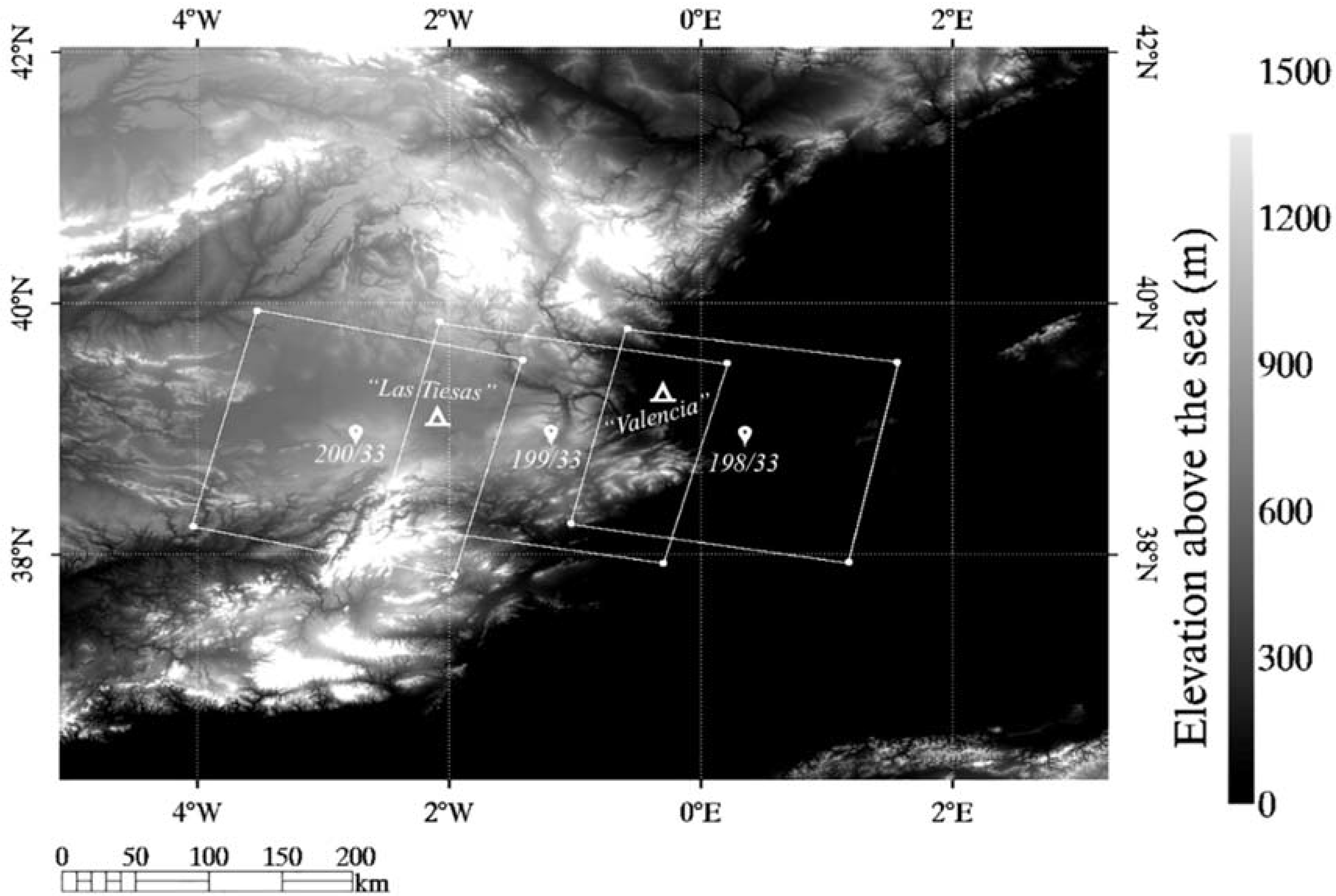
2.4. Satellite Images
3. Results and Discussion
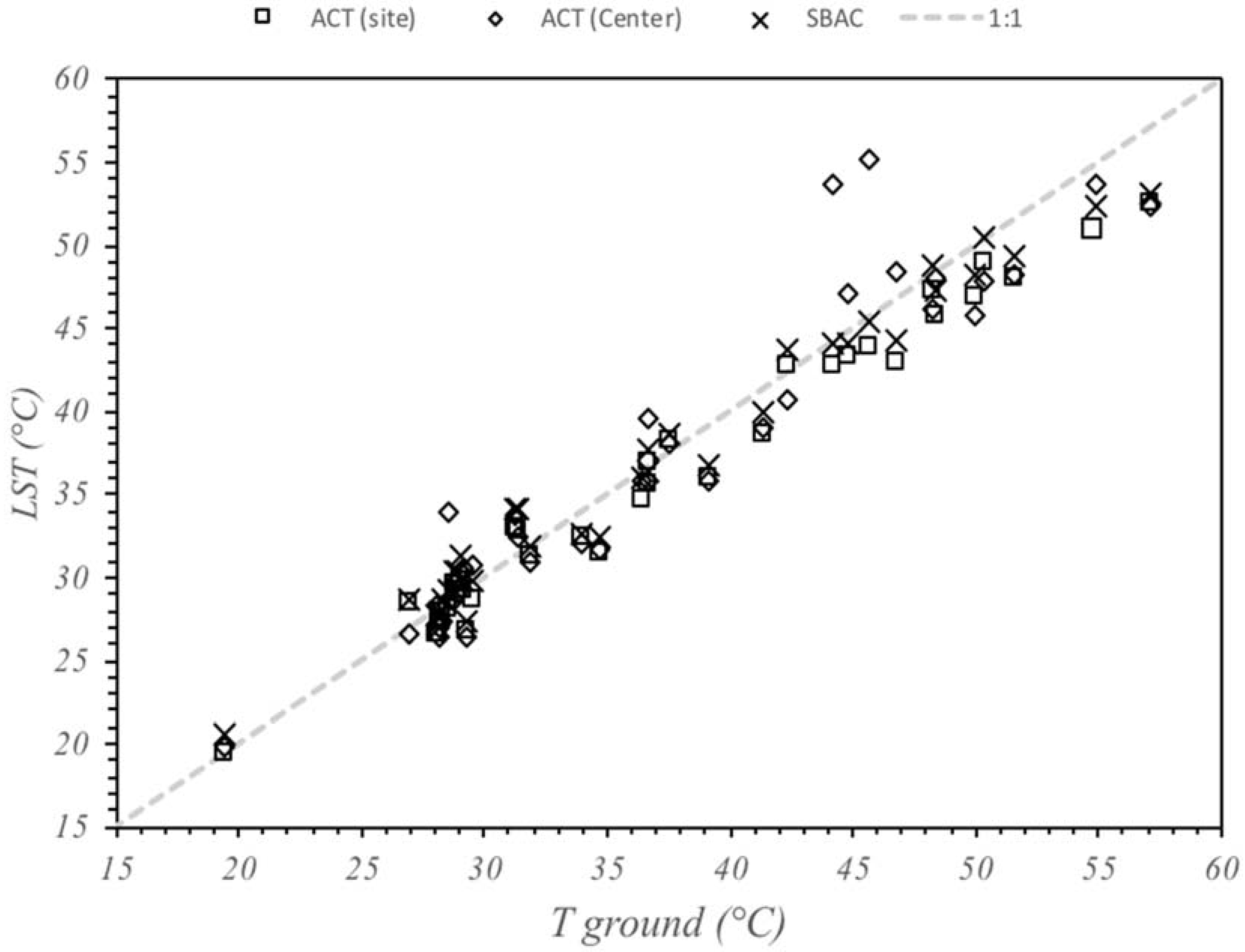
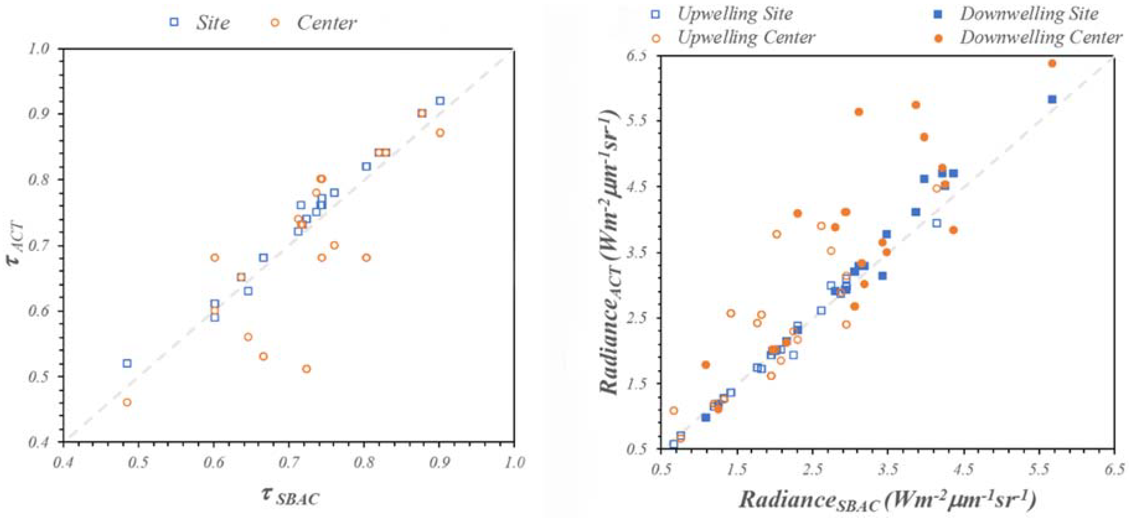
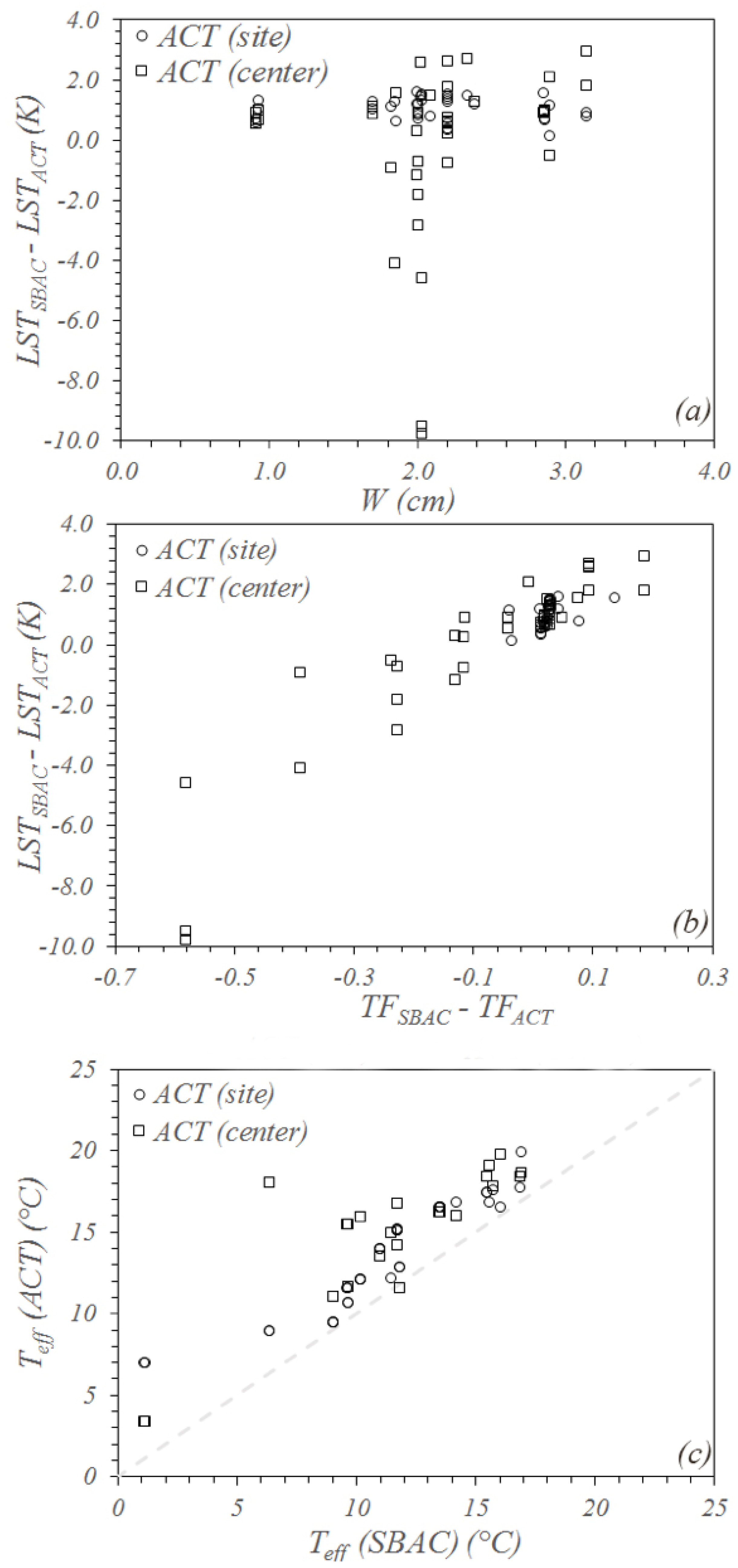
3.1. Local Validation of SBAC
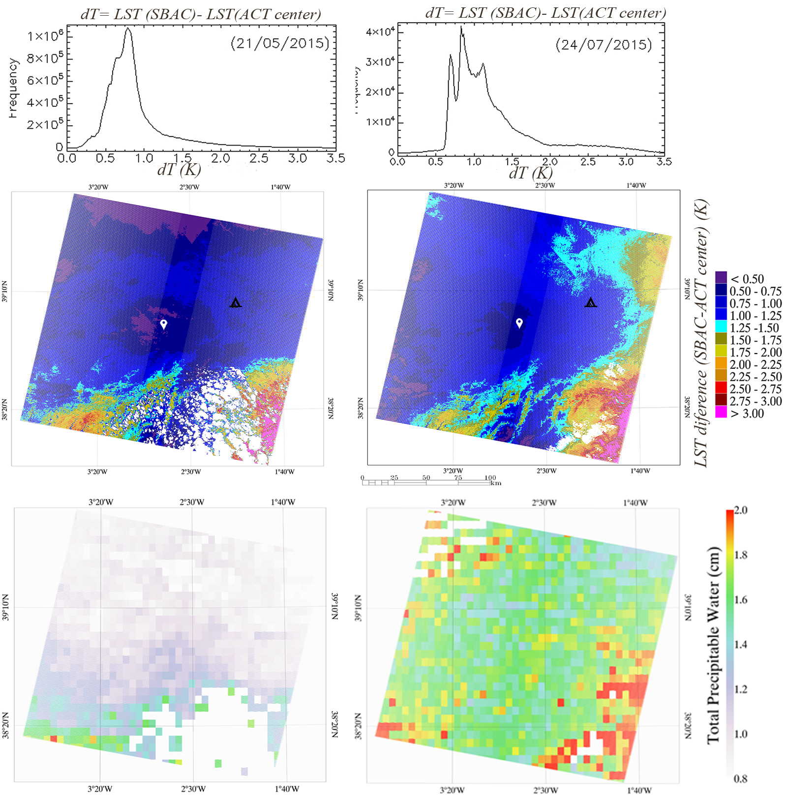
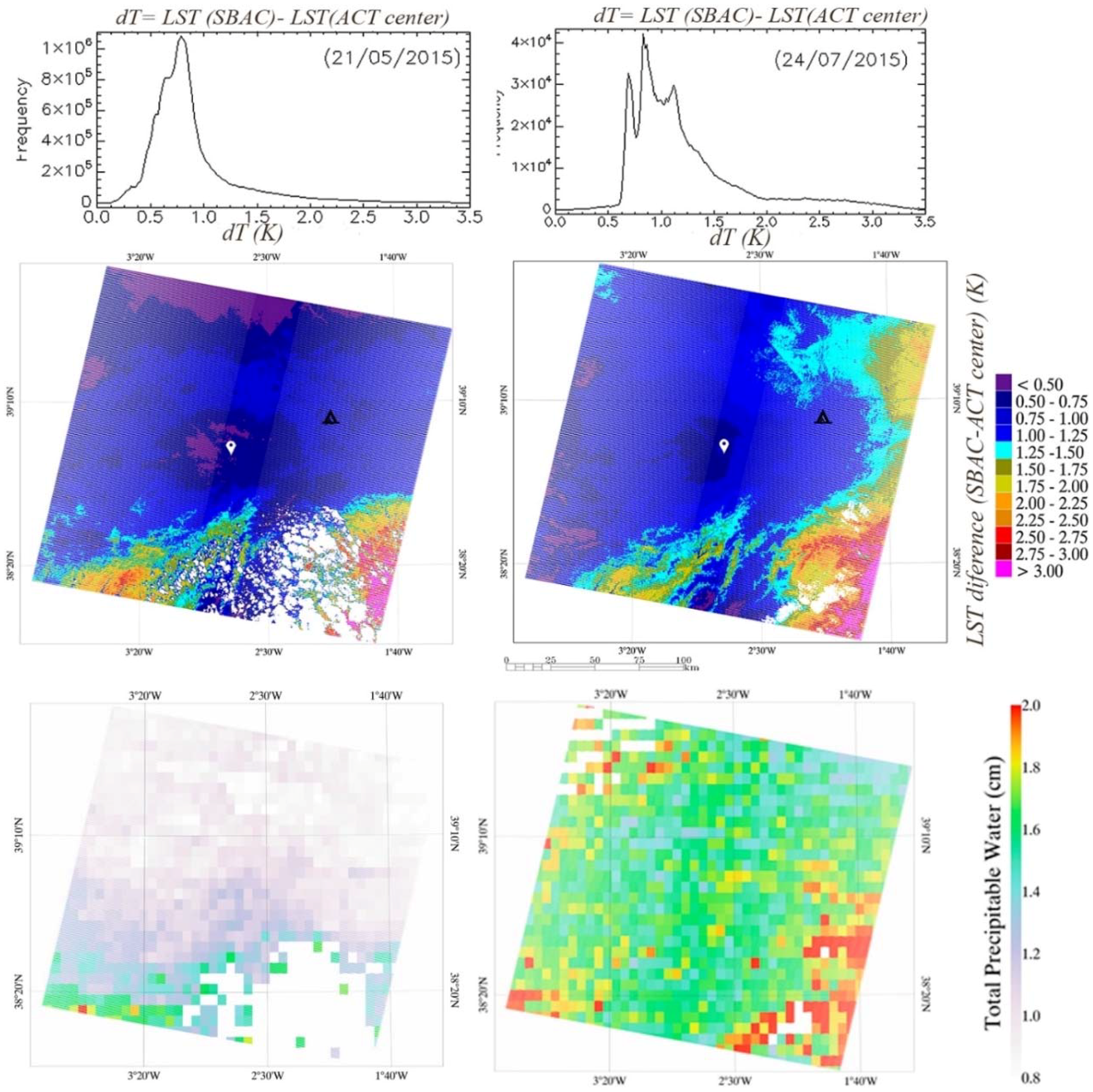
3.2. Full-Scene Analysis of SBAC Tool Outputs
4. Conclusions
Author Contributions
Acknowledgments
Conflicts of Interest
References
- Allen, R.G.; Tasumi, M.; Trezza, R. Satellite-based energy balance for mapping evapotranspiration with internalized calibration (METRIC)-model. J. Irrig. Drain. Eng. 2007, 133, 380–394. [Google Scholar] [CrossRef]
- Sánchez, J.M.; Caselles, V.; Niclòs, R.; Coll, C.; Kustas, W.P. Estimating energy balance fluxes above a boreal forest from radiometric temperature observations. Agric. For. Meteorol. 2009, 149, 1037–1049. [Google Scholar] [CrossRef]
- Sánchez, J.M.; López-Urrea, R.; Doña, C.; Caselles, V.; González-Piqueras, J.; Niclòs, R. Modeling evapotranspiration in a spring wheat from thermal radiometry: Crop coefficients and E/T partitioning. Irrig. Sci. 2015, 33, 399–410. [Google Scholar] [CrossRef]
- Weng, Q. Thermal infrared remote sensing for urban climate and environmental studies: Methods, applications, and trends. ISPRS J. Photogramm. Remote. Sens. 2009, 64, 335–344. [Google Scholar] [CrossRef]
- Tomlinson, C.J.; Chapman, L.; Thornes, J.E.; Baker, C. Remote sensing land surface temperature for meteorology and climatology: A review. Meteorol. Appl. 2011, 18, 296–306. [Google Scholar] [CrossRef]
- Li, Z.-L.; Tang, B.-H.; Wu, H.; Ren, H.; Yan, G.; Wan, Z.; Trigo, I.F.; Sobrino, J.A. Satellite-derived land surface temperature: Current status and perspectives. Remote Sens. Environ. 2013, 131, 14–37. [Google Scholar] [CrossRef]
- Anderson, M.C.; Allen, R.G.; Morse, A.; Kustas, W.P. Use of Landsat thermal imagery in monitoring evapotranspiration and managing water resources. Remote Sens. Environ. 2012, 122, 50–65. [Google Scholar] [CrossRef]
- Miralles, D.G.; Teuling, A.J.; van Heerwaarden, C.C.; de Arellano, J.V. Mega-heatwave temperatures due to combined soil desiccation and atmospheric heat accumulation. Nat. Geosci. 2014, 7, 345–349. [Google Scholar] [CrossRef]
- Ramsey, M.S.; Harris, A.J.L. Volcanology 2020: How will thermal remote sensing of volcanic activity evolve over the next decade. J. Volcanol. Geotherm. Res. 2013, 249, 217–233. [Google Scholar] [CrossRef]
- Voogt, J.A.; Oke, T.R. Thermal remote sensing of urban climates. Remote Sens. Environ. 2003, 86, 370–384. [Google Scholar] [CrossRef]
- Price, J.C. Land surface temperature measurements from the split-window channels of the NOAA 7 AVHRR. J. Geophys. Res. 1984, 89, 7231–7237. [Google Scholar] [CrossRef]
- Becker, F.; Li, Z.-L. Towards a local split-window method over land surfaces. Int. J. Remote Sens. 1990, 11, 369–394. [Google Scholar] [CrossRef]
- Becker, F.; Li, Z.-L. Surface temperature and emissivity at various scales: Definition, measurement and related problems. Remote Sens. Environ. 1995, 12, 225–253. [Google Scholar] [CrossRef]
- Coll, C.; Caselles, V. A split-window algorithm for land surface temperature from Advance Very High Resolution Radiometer data: Validation and algorithm comparison. J. Geophys. Res. 1997, 102, 16697–16713. [Google Scholar] [CrossRef]
- Wan, Z. MODIS Land Surface Temperature. Algorithm Theoretical Basis Document; NAS5-31370; University of California: Santa Barbara, CA, USA, 1999. [Google Scholar]
- Wan, Z. New refinements and validation of the MODIS Land-Surface Temperature/Emissivity products. Remote Sens. Environ. 2008, 112, 59–74. [Google Scholar] [CrossRef]
- Galve, J.M.; Coll, C.; Caselles, V.; Valor, E. An atmospheric radiosounding database for generating land surface temperature algorithms. IEEE Trans. Geosci. Remote Sens. 2008, 46, 1547–1557. [Google Scholar] [CrossRef]
- Prata, A.J. Land Surface Temperature Measurement from Space: AATSR Algorithm Theoretical Basis Document; Tech. Rep. 34; CSIRO Atmospheric Research: Aspendale, Australia, 2002. [Google Scholar]
- Madeira, C. Generalized split-window algorithm for retrieving land surface temperature from MSG/SEVIRI data. In Proceedings of the Land Surface Analysis SAF Training Workshop, Lisbon, Portugal, 8–10 July 2002; pp. 42–47. [Google Scholar]
- Trigo, I.T.; Monteiro, F.; Olesen, E.; Kabsch, E. An assessment of remotely sensed land surface temperature. J. Geophys. Res. 2008, 113, D17108. [Google Scholar] [CrossRef]
- Niclòs, R.; Galve, J.M.; Valiente, J.A.; Estrela, M.J.; Coll, C. Accuracy assessment of land surface temperature retrievals from MSG2-SEVIRI data Rem. Sens. Environ. 2011, 115, 2126–2140. [Google Scholar] [CrossRef]
- Yu, Y.; Privette, J.L.; Pinheiro, A. Analysis of the NPOESS VIIRS land surface temperature algorithm using MODIS data. IEEE Trans. Geosci. Remote Sens. 2005, 43, 2340–2350. [Google Scholar]
- Niclòs, R.; Pérez-Planells, L.; Coll, C.; Valiente, J.A.; Valor, E. Evaluation of the S-NPP VIIRS land surface temperature product using ground data acquired by an autonomous system at a rice paddy. ISPRS J. Photogramm. Remote Sens. 2018, 135, 1–12. [Google Scholar] [CrossRef]
- Gillespie, A.R.; Matsunaga, T.; Rokugawa, S.; Hook, S.J. Temperature and emissivity separation from Advanced Spaceborne Thermal Emission and Reflection Radiometer (ASTER) images. IEEE Trans. Geosci. Remote Sens. 1998, 36, 1113–1125. [Google Scholar] [CrossRef]
- Coll, C.; Caselles, V.; Valor, E.; Niclòs, R.; Sánchez, J.M.; Galve, J.M.; Mira, M. Temperature and emissivity separation from ASTER data for low spectral contrast surfaces. Remote Sens. Environ. 2007, 110, 162–175. [Google Scholar] [CrossRef]
- Hulley, G.; Hook, S.; Hughes, C. MODIS MOD21 Land Surface Temperature and Emissivity Algorithm Theoretical Basis Document; Jet Propulsion Lab., California Inst. Technol.: Pasadena, CA, USA, 12–17 August 2012; (updated: March 2014). [Google Scholar]
- Coll, C.; Garca-Santos, V.; Niclòs, R.; Caselles, V. Test of the MODIS land surface temperature and emissivity separation algorithm with ground measurements over a rice paddy. IEEE Trans. Geosci. Remote Sens. 2016, 54, 3061–3069. [Google Scholar] [CrossRef]
- Coll, C.; Caselles, V.; Valor, E.; Niclòs, R. Comparison between different sources of atmospheric profiles for land surface temperature retrieval from single channel thermal infrared data. Remote Sens. Environ. 2012, 117, 199–210. [Google Scholar] [CrossRef]
- Li, H.; Liu, Q.; Du, Y.; Jiang, J.; Wang, H. Evaluation of the NCEP and MODIS atmospheric products for single channel land surface temperature retrieval with ground measurements: A case study of HJ-1B IRS data. IEEE J. Sel. Top. Appl. Earth Observ. Remote Sens. 2013, 6, 1399–1408. [Google Scholar] [CrossRef]
- Meng, X.; Cheng, J. Evaluating Eight Global Reanalysis Products for Atmospheric Correction of Thermal Infrared Sensor—Application to Landsat 8 TIRS10 Data. Remote Sens. 2018, 10, 474. [Google Scholar] [CrossRef]
- Duan, S.-B.; Li, Z.-L.; Wang, C.; Zhang, S.; Tang, B.-H.; Leng, P.; Gao, M.-F. Land-surface temperature retrieval from Landsat 8 single-channel thermal infrared data in combination with NCEP reanalysis data and ASTER GED product. Int. J. Remote Sens. 2018. [Google Scholar] [CrossRef]
- Barsi, J.A.; Barker, J.L.; Schott, J.R. An Atmospheric Correction Parameter Calculator for a Single Thermal Band Earth-Sensing Instrument. In Proceedings of the Geoscience and Remote Sensing Symposium 2003 (IGARSS ’03), Toulouse, France, 21–25 July 2003. [Google Scholar]
- Barsi, J.A.; Schott, J.R.; Palluconi, F.D.; Hook, S.J. Validation of a Web-Based Atmospheric Correction Tool for Single Thermal Band Instruments. In Proceedings of the Earth Observing Systems X, San Diego, CA, USA, 22 August 2005; Volume 5882. [Google Scholar]
- Coll, C.; Galve, J.M.; Sánchez, J.M.; Caselles, V. Validation of landsat-7/ETM+ thermal-band calibration and atmospheric correction with ground-based measurements. IEEE Trans. Geosci. Remote Sens. 2010, 48, 547–555. [Google Scholar] [CrossRef]
- Tardy, B.; Rivalland, V.; Huc, M.; Hagolle, O.; Marcq, S.; Boulet, G. A software tool for atmospheric correction and surface temperature estimation of landsat infrared thermal data. Remote Sens. 2016, 8, 696. [Google Scholar] [CrossRef] [Green Version]
- Berk, A.; Anderson, G.P.; Acharya, P.K.; Shettle, E.P. MODTRAN 5.2.1 User’s Manual; Spectral Sciences, Inc.: Burlington, MA, USA, 2011. [Google Scholar]
- Kalnay, E.; Kanamitsu, M.; Kistler, R.; Collins, W.; Deaven, D.; Gandin, L.; Iredell, M.; Saha, S.; White, G.; Woollen, J.; et al. The NCEP/NCAR 40 year reanalysis project. Bull. Am. Meteorol. Soc. 1996, 77, 437–471. [Google Scholar] [CrossRef]
- García-Santos, V.; Valor, E.; Caselles, V.; Mira, M.; Galve, J.M.; Coll, C. Evaluation of different methods to retrieve the hemispherical downwelling irradiance in the thermal infrared region for field measurements. IEEE Trans. Geosci. Remote Sens. 2013, 51, 2155–2165. [Google Scholar] [CrossRef]
- Wan, Z.; Dozier, J. Land-surface temperature measurement from space: Physical principles and inverse modeling. IEEE Trans. Geosci. Remote Sens. 1989, 27, 268–277. [Google Scholar]
- Richter, R.; Coll, C. Band-pass resampling effects for the retrieval of surface emissivity. Appl. Opt. 2002, 41, 3523–3529. [Google Scholar] [CrossRef] [PubMed]
- Valor, E.; Caselles, V. Mapping Land Surface Emissivity from NDVI: Application to European, African and South American Areas. Remote Sens. Environ. 1996, 57, 167–184. [Google Scholar] [CrossRef]
- Valor, E.; Caselles, V. Validation of the vegetation cover method for land surface emissivity estimation. In Recent Research Developments in Thermal Remote Sensing; Research Singpost: Kerala, India, 2005; pp. 1–20. [Google Scholar]
- Duchemin, B.; Hadria, R.; Er-Raki, S.; Boulet, G.; Maisongrande, P.; Chehbouni, A.; Escadafal, R.; Ezzahar, J.; Hoedjes, J.C.B.; Kharrou, M.H.; et al. Monitoring wheat phenology and irrigation in central Morocco on the use of relationships between evapotranspiration, crop coefficients, leaf area index and remotely-sensed vegetation indices. Agric. Water Manag. 2006, 79, 1–27. [Google Scholar] [CrossRef]
- Asrar, G.; Fuchs, M.; Kanemasu, E.T.; Hatfield, J.L. Estimating absorbed photosynthetic radiation and leaf area index from spectral reflectance in wheat. Agron. J. 1984, 76, 300–306. [Google Scholar] [CrossRef]
- Berk, A.; Anderson, G.P.; Acharya, P.K.; Bernstein, L.S.; Muratov, L.; Lee, J.; Fox, M.; Adler-Golden, S.M.; Chetwynd, J.H.; Hoke, M.L.; et al. MODTRAN5: 2006 Update. In Proceedings of the Volume 6233, Algorithms and Technologies for Multispectral, Hyperspectral, and Ultraspectral Imagery XII, Kissimmee, FL, USA, 8 May 2006. [Google Scholar] [CrossRef]
- Shepard, D. A two-dimensional interpolation function for irregularly-spaced data. In Proceedings of the 1968 23rd ACM National Conference, Princeton, NJ, USA, 27–29 August 1968; ACM: New York, NY, USA, 1968; pp. 517–524. [Google Scholar]
- Sobrino, J.A.; Jiménez-Muñoz, J.C.; Sòria, G.; Romaguera, M.; Guanter, L.; Moreno, J.; Plaza, A.; Martínez, P. Land surface emissivity retrieval from different VNIR and TIR sensors. IEEE Trans. Geosci. Remote Sens. 2008, 46, 316–327. [Google Scholar] [CrossRef]
- Moreno, J.F.; Alonso, L.; Fernàndez, G.; Fortea, J.C.; Gandía, S.; Guanter, L.; Garcia, J.C.; Martí, J.M.; Melia, J.; De Coca, F.C.; et al. The SPECTRA Barrax campaign (SPARC): Overview and First Results from CHRIS Data; Special Publication; European Space Agency: Paris, France, 2004; Volume 578, pp. 30–39. [Google Scholar]
- Latorre, C.; Camacho, F.; de la Cruz, F.; Lacaze, R.; Weiss, M.; Baret, F. Seasonal monitoring of FAPAR over the Barrax cropland site in Spain in support of the validation of PROBA-V products at 333 m. In Proceedings of the Fourth Recent Advances in Quantitative Remote Sensing, Torrent, Spain, 22–26 September 2014; pp. 431–435. [Google Scholar]
- Berger, M.; Rast, M.; Wursteisen, P.; Attema, E.; Moreno, J.; Müller, A.; Beisl, U.; Richter, R.; Schaepman, M.; Strub, G.; et al. The DAISEX Campaigns in Support of a Future Land-Surface-Processes Mission; ESA Bulletin: Paris, France, 2011; pp. 101–111. ISSN 0376-4265. [Google Scholar]
- López-Urrea, R.; de Santa Martín, F.M.; Olalla, F.; Fabeiro, C.; Moratalla, A. Testing evapotranspiration equations using lysimeter observations in a semiarid climate. Agric. Water Manag. 2006, 85, 15–26. [Google Scholar] [CrossRef]
- López-Urrea, R.; Montoro, A.; González-Piqueras, J.; López-Fuster, P.; Fereres, E. Water use of spring wheat to raise water productivity. Agric. Water Manag. 2009, 96, 1305–1310. [Google Scholar] [CrossRef]
- López-Urrea, R.; Montoro, A.; Mañas, F.; López-Fuster, P.; Fereres, E. Evapotranspiration and crop coefficients from lysimeter measurements of mature ‘Tempranillo’ wine grapes. Agric. Water Manag. 2012, 112, 13–20. [Google Scholar]
- Sánchez, J.M.; López-Urrea, R.; Rubio, E.; Caselles, V. Determining water use of sorghum from two-source energy balance and radiometric temperatures. Hydrol. Earth Syst. Sci. 2011, 15, 3061–3070. [Google Scholar] [CrossRef] [Green Version]
- Sánchez, J.M.; López-Urrea, R.; Rubio, E.; González-Piqueras, J.; Caselles, V. Assessing crop coefficients of sunflower and canola using two-source energy balance and thermal radiometry. Agric. Water Manag. 2014, 137, 23–29. [Google Scholar] [CrossRef]
- Sánchez, J.M.; French, A.N.; Mira, M.; Hunsaker, D.J.; Thorp, K.R.; Valor, E.; Caselles, V. Thermal infrared emissivity dependence on soil moisture in field conditions. IEEE Trans. Geosci. Remote Sens. 2011, 49, 4652–4659. [Google Scholar] [CrossRef]
- Gao, B. MODIS Atmosphere L2 Water Vapor Product; NASA MODIS Adaptive Processing System, Goddard Space Flight Center: Greenbelt, MD, USA, 2015. [Google Scholar] [CrossRef]
- Barsi, J.A.; Schott, J.R.; Palluconi, F.D.; Helder, D.L.; Hook, S.J.; Markham, B.L.; Chander, G.; O’Donnell, E.M. Landsat TM and ETM+ thermal band calibration. Can. J. Remote Sens. 2003, 29, 141–153. [Google Scholar] [CrossRef]
- Coll, C.; Caselles, V.; Sobrino, J.A.; Valor, E. On the atmospheric dependence of the split-window equation for land surface temperature. Int. J. Remote Sens. 1994, 15, 105–122. [Google Scholar] [CrossRef]


| # | Date | Path | Row | Crop | Extension | Latitude | Longitude | Altitude |
|---|---|---|---|---|---|---|---|---|
| (ha) | (°) | (°) | (km) | |||||
| 1 | 12/08/2004 | 198 | 33 | Rice | >100 | 39.250 | −0.295 | 0.007 |
| 2 | 21/07/2005 | 199 | 33 | Rice | >100 | 39.265 | −0.308 | 0.006 |
| 3 | 06/08/2005 | 199 | 33 | Rice | >100 | 39.265 | −0.308 | 0.006 |
| 4 | 24/07/2006 | 199 | 33 | Rice | >100 | 39.265 | −0.308 | 0.006 |
| 5 | 02/08/2006 | 198 | 33 | Rice | >100 | 39.265 | −0.308 | 0.006 |
| 6 | 11/07/2007 | 199 | 33 | Rice | >100 | 39.265 | −0.308 | 0.006 |
| 7 | 20/07/2007 | 198 | 33 | Rice | >100 | 39.265 | −0.308 | 0.006 |
| 8 | 21/05/2015 | 200 | 33 | Barley | 25.4 | 39.059 | −2.099 | 0.694 |
| 9 | Vineyard | 5.0 | 39.060 | −2.101 | 0.692 | |||
| 10 | 22/06/2015 | 200 | 33 | Barley | 25.4 | 39.059 | −2.099 | 0.694 |
| 11 | Corn | 25.4 | 39.059 | −2.096 | 0.693 | |||
| 12 | 01/07/2015 | 199 | 33 | Barley | 25.4 | 39.059 | −2.099 | 0.694 |
| 13 | Corn | 25.4 | 39.059 | −2.096 | 0.693 | |||
| 14 | Vineyard | 5.0 | 39.060 | −2.101 | 0.692 | |||
| 15 | 17/07/2015 | 199 | 33 | Barley | 25.4 | 39.059 | −2.099 | 0.694 |
| 16 | Corn | 25.4 | 39.059 | −2.096 | 0.693 | |||
| 17 | 24/07/2015 | 200 | 33 | Corn | 25.4 | 39.059 | −2.096 | 0.693 |
| 18 | Vineyard | 5.0 | 39.060 | −2.101 | 0.692 | |||
| 19 | 02/08/2015 | 199 | 33 | Corn | 25.4 | 39.059 | −2.096 | 0.693 |
| 20 | Vineyard | 5.0 | 39.060 | −2.101 | 0.692 | |||
| 21 | 09/08/2015 | 200 | 33 | Corn | 25.4 | 39.059 | −2.096 | 0.693 |
| 22 | Vineyard | 5.0 | 39.060 | −2.101 | 0.692 | |||
| 23 | 18/08/2015 | 199 | 33 | Barley | 25.4 | 39.059 | −2.099 | 0.694 |
| 24 | Corn | 25.4 | 39.059 | −2.096 | 0.693 | |||
| 25 | Vineyard | 5.0 | 39.060 | −2.101 | 0.692 | |||
| 26 | 01/06/2016 | 199 | 33 | Garlic | 25.4 | 39.059 | −2.099 | 0.694 |
| 27 | Garlic | 25.4 | 39.059 | −2.096 | 0.693 | |||
| 28 | 24/06/2016 | 200 | 33 | Garlic | 25.4 | 39.059 | −2.099 | 0.694 |
| 29 | Garlic | 25.4 | 39.059 | −2.096 | 0.693 | |||
| 30 | Barley | 54.4 | 39.056 | −2.080 | 0.692 | |||
| 31 | 19/07/2016 | 199 | 33 | Vineyard | 5.0 | 39.060 | −2.101 | 0.691 |
| 32 | Garlic | 25.4 | 39.059 | −2.099 | 0.694 | |||
| 33 | 26/07/2016 | 200 | 33 | Almonds | 11.1 | 39.043 | −2.090 | 0.692 |
| 34 | Vineyard | 5.0 | 39.060 | −2.101 | 0.692 | |||
| 35 | Barley | 11.1 | 39.057 | −2.088 | 0.695 | |||
| 36 | Wet Bare Soil | 25.4 | 39.058 | −2.098 | 0.689 |
| # | Tg | ±σ | W | ε | Tb | # | Tg | ±σ | W | ε | Tb |
|---|---|---|---|---|---|---|---|---|---|---|---|
| (°C) | (°C) | (cm) | (°C) | (°C) | (°C) | (cm) | (°C) | ||||
| 1 | 28.2 | 0.6 | 2.1 | 0.988 | 24.9 | 19 | 29.5 | 0.6 | 1.8 | 0.988 | 25.1 |
| 2 | 28.1 | 0.4 | 2.0 | 0.988 | 24.4 | 20 | 46.7 | 1.9 | 1.9 | 0.978 | 35.2 |
| 3 | 28.1 | 0.5 | 1.9 | 0.988 | 24.4 | 21 | 28.7 | 0.3 | 3.1 | 0.990 | 23.1 |
| 4 | 28.8 | 0.4 | 2.4 | 0.988 | 24.9 | 22 | 42.3 | 0.3 | 3.1 | 0.967 | 31.1 |
| 5 | 29.0 | 0.9 | 2.9 | 0.988 | 23.9 | 23 | 45.5 | 3.4 | 2.0 | 0.975 | 35.6 |
| 6 | 26.9 | 0.5 | 2.9 | 0.988 | 21.8 | 24 | 28.4 | 0.3 | 2.0 | 0.989 | 24.5 |
| 7 | 28.0 | 0.4 | 2.9 | 0.988 | 22.8 | 25 | 44.1 | 1.4 | 2.0 | 0.980 | 35.6 |
| 8 | 19.4 | 0.9 | 0.9 | 0.986 | 17.8 | 26 | 36.6 | 2.6 | 0.9 | 0.990 | 33.2 |
| 9 | 41.3 | 2.7 | 0.9 | 0.970 | 34.2 | 27 | 29.2 | 1.8 | 0.9 | 0.991 | 25.2 |
| 10 | 39.0 | 0.9 | 2.9 | 0.977 | 29.9 | 28 | 57.1 | 2.4 | 2.2 | 0.965 | 44.4 |
| 11 | 31.9 | 1.1 | 2.9 | 0.992 | 25.5 | 29 | 33.8 | 2.1 | 2.2 | 0.987 | 28.5 |
| 12 | 36.6 | 0.5 | 2.0 | 0.977 | 31.3 | 30 | 37.4 | 1.3 | 2.2 | 0.975 | 32.8 |
| 13 | 29.0 | 0.3 | 2.0 | 0.989 | 26.0 | 31 | 48.3 | 0.8 | 2.2 | 0.973 | 38.4 |
| 14 | 44.8 | 1.3 | 2.0 | 0.977 | 37.1 | 32 | 36.4 | 2.3 | 2.2 | 0.969 | 30.1 |
| 15 | 54.9 | 1.8 | 2.0 | 0.972 | 42.7 | 33 | 50.3 | 1.6 | 2.3 | 0.966 | 40.5 |
| 16 | 31.2 | 3.6 | 2.0 | 0.989 | 27.9 | 34 | 48.2 | 1.1 | 2.2 | 0.973 | 39.4 |
| 17 | 34.6 | 0.4 | 1.7 | 0.989 | 29.0 | 35 | 49.9 | 2.3 | 2.0 | 0.968 | 39.5 |
| 18 | 51.6 | 0.8 | 1.7 | 0.968 | 41.6 | 36 | 31.3 | 0.8 | 2.2 | 0.967 | 28.1 |
© 2018 by the authors. Licensee MDPI, Basel, Switzerland. This article is an open access article distributed under the terms and conditions of the Creative Commons Attribution (CC BY) license (http://creativecommons.org/licenses/by/4.0/).
Share and Cite
Galve, J.M.; Sánchez, J.M.; Coll, C.; Villodre, J. A New Single-Band Pixel-by-Pixel Atmospheric Correction Method to Improve the Accuracy in Remote Sensing Estimates of LST. Application to Landsat 7-ETM+. Remote Sens. 2018, 10, 826. https://doi.org/10.3390/rs10060826
Galve JM, Sánchez JM, Coll C, Villodre J. A New Single-Band Pixel-by-Pixel Atmospheric Correction Method to Improve the Accuracy in Remote Sensing Estimates of LST. Application to Landsat 7-ETM+. Remote Sensing. 2018; 10(6):826. https://doi.org/10.3390/rs10060826
Chicago/Turabian StyleGalve, Joan M., Juan M. Sánchez, César Coll, and Julio Villodre. 2018. "A New Single-Band Pixel-by-Pixel Atmospheric Correction Method to Improve the Accuracy in Remote Sensing Estimates of LST. Application to Landsat 7-ETM+" Remote Sensing 10, no. 6: 826. https://doi.org/10.3390/rs10060826