A Study of a Generalized Photovoltaic System with MPPT Using Perturb and Observer Algorithms under Varying Conditions

Abstract

In recent years, renewable energy (RE) has shown promise as a sustainable solution to the rising energy demand worldwide. Photovoltaic (PV) technology has emerged as a highly viable RE alternative. The majority of PV schemes use specific PV models with specified parameters. This study proposes a PV model with generic specifications, a PV array, a DC/DC converter, a DC/AC inverter, maximum power point tracking (MPPT), and grid synchronization using a feedback control system under the MATLAB/Simulink environment. Various MPPT techniques have been adapted to track the PV’s maximum power point (MPP); however, there are various uncertainties. To address these challenges, this paper presented a perturb and observe (P&O) strategy to track the MPP of PV systems reliably. The MPP of a PV system varies according to meteorological order, such as solar radiation and cell temperature. The MPPT primarily gathers the maximum current and voltage of the PV array and provides them to the load using a boost converter. The MPPT performance and PV array attributes are analyzed during abrupt weather changes. Finally, a feedback controller is configured to perform synchronization of the inverter with the grid. The validity and reliability of the PV module using P&O methods provide a higher efficacy of MPPT under MATLAB/simulation. Finally, the presented results endorse the strength of the proposed technique.

1. Introduction

The rapid increase in energy demand with the variation in atmospheric conditions has intensified the importance of renewable energy resources (RERs) for sustainable development. RERs are based on natural sources such as wind, sunlight, tides, etc. These are economical and viable with less carbon emissions and can be certainly replenished [1,2,3,4]. Among several RERs, solar energy is an abundant and easily available source. Solar energy has provided many favorable avenues to solve problems in the power sector [5,6,7]. Solar energy is highly dependent on meteorological factors, including solar radiation and temperature, and as a result, it changes constantly. Due to this, solar PV energy has an intermittent character in nature [8,9].

The photovoltaic (PV) modules’ output features are influenced by solar radiation and the temperature of cells, and are enlightened in [10]. The nonlinear electrical attributes of PV modules make PV modelling essential in designing and simulating PV systems. To increase the efficiency and adaptability of PV systems, several models have been proposed [11]. R. Falinirina presented a system emphasizing PV systems, the modelling and simulation of PV arrays, maximum power point tracking (MPPT) control, and DC/DC converters [7,12]. The operating potential of the studied system was analyzed and evaluated using MATLAB. However, synchronization with the grid is yet to be considered. Lipika et al. presented an optimized perturb and observer (P&O) technique using a buck–boost converter to analyze PV module tracking performance [13,14]. In [13], the presented control system adjusted the voltage level by using small amounts from the PV array and power measures; if the power increases, further adjustments in that direction are tried until there is no longer an increase in power. However, optimization regarding system efficiency was performed using a P&O algorithm via adopting a buck–boost converter and changing the duty cycle of the boost–buck. The source impedance was matched by adjusting the impedance of the load to enhance system performance. In addition, a MATLAB/Simulink-based model was used to adapt the PV energy case study. The authors implemented two types of MPPT controllers to compare the effectiveness of both controllers for PV systems. The proposed system has numerous advantages, it is simple, reliable, permits the simulation of cells, etc., and it also analyses incompatible panels which operate under different conditions [15].

The world is looking towards harnessing its solar resources as an alternative energy source to overcome the continuous power shortages and unreliable power supply. To achieve maximum power output, optimizing the system components of the photovoltaic system is essential. Further, the P&O technique still contains several drawbacks in the MPPT of solar PV installation. These include sustained oscillation around the MPP, a tradeoff between fast tracking and instability, and the requirement for users to define constants beforehand. The major limitation of the P&O method is the potential for oscillations, which can occur when the process overshoots the MPP and then corrects itself in the opposite direction. In addition, steady-state oscillations occur during fast-varying environmental conditions and due to the difficulty of step size control. These oscillations can result in a fluctuating output power that can decrease the system’s overall efficiency. These limitations can be erased by using data analytic algorithms with a feedback loop strategy.

Another limitation of the P&O method is its sensitivity to step size. The step size determines the amount of change in the operating point at each iteration, and if the step size is too large, it can lead to oscillations or even failure to converge to the MPP. On the other hand, if the step size is too small, it can lead to slow convergence and increased computational time of the system.

Several modifications have been proposed to address these limitations to improve the performance of the P&O method. One approach is to use a modified P&O strategy that includes a hysteresis band to prevent oscillations. This technique adjusts the reference voltage only when the PV module output power exceeds a specific range of values; otherwise, it maintains the previous reference voltage to maintain constant operation.

The basic premise of this study is to propose a PV model incorporating a PV module with broad parameters, a PV array, a P&O-algorithm-based MPPT, a DC/DC converter, a DC/AC inverter, and synchronization with the grid using a feedback controller under MATLAB/Simulink software. MATLAB/Simulink provides an intelligent, modular, and graphical simulation environment for the constantly varying scrutiny of power systems. It also helps in the design and simulation of the power system. This study presents an improved PV system compared to the work using an artificial neural network studied in [16]. This paper includes PV modeling with generic parameters. The generic PV model provides a user-friendly interface to define various PV parameters. This capability enables the users to analyze the PV system using any type of PV module.

Considering the subject under study, the primary purpose of this study is to present a simple and adaptive way to meet maximum output in the solar cell in various environmental conditions using the P&O algorithm. The prototype should be simple with high efficiency. The proposed method offers a generalized approach to tracking the MPP in photovoltaic systems adaptively. It eliminates steady-state oscillations around the MPP and does not necessitate system-dependent constants. As a result, this technique provides a general foundation for designing various types of PV systems with MPPT using a space vector pulse width modulation (SVPWM). This paper includes PV modeling with generic parameters. The generic PV model offers a user-friendly interface to define different PV parameters. This capability enables the users to analyze the PV system with any PV module. In parallel, a DC/DC converter, along with the MPPT controller, has been implemented. The results illustrate that MPPT in the PV module effectively tracks the MPPT in terms of the current and voltage of the PV array under sudden deviations in solar irradiance, temperature, and variable load events. The second significant contribution of this study is the implementation of PV system synchronization with the primary grid [17]. This study implemented a three-phase inverter and synchronized it with the grid, adapting a feedback SVPWM technique.

The organization of this paper is as follows: Section 2 describes the proposed system model with the implemented algorithm. The presented system simulation model is presented in Section 3. The test system simulation results and discussion are provided in Section 4. Finally, the conclusion is drawn in Section 5. A short version of this study has been published as a conference paper in [18].

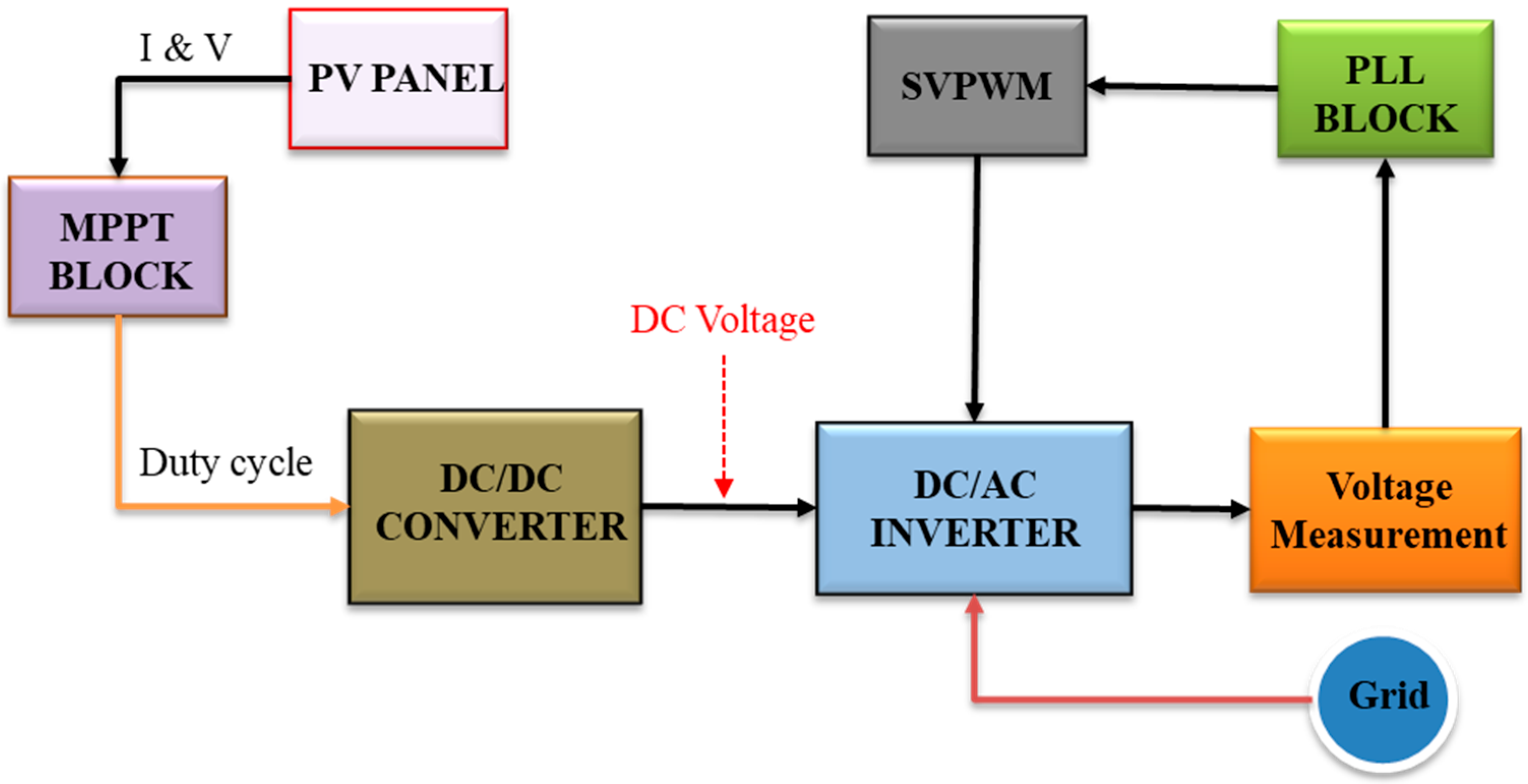
2. The Proposed Model

This section is dedicated to details of the studied generalized PV system. The implemented system comprises five major subsystems, including a PV system model, a DC/DC converter, an MPPT controller, a DC/AC inverter, and a grid synchronization module. The synchronization module comprises SVPWM, phase-locked loop (PLL), and voltage measurement modules. The structural outline of the proposed logic is described in Figure 1. The PV panel utilizes solar irradiance and temperature as inputs and generates outputs in the form of a current (I) and voltage (V). The MPPT controller tracks the MPP of the PV panel using the P&O algorithm. Parallel to this, the DC/DC converter boosts the output DC voltage and feeds it to a DC/AC inverter, which renovates the DC output into AC. The grid synchronization module is designed to integrate the DC/AC inverter output with the grid. The PLL block generates a reference signal with the same frequency and angle as the grid and provides them to the SVPWM system as input. SVPWM is a modulation technique that generates controlled gating signals for the inverter by operating as a feedback loop system [19].

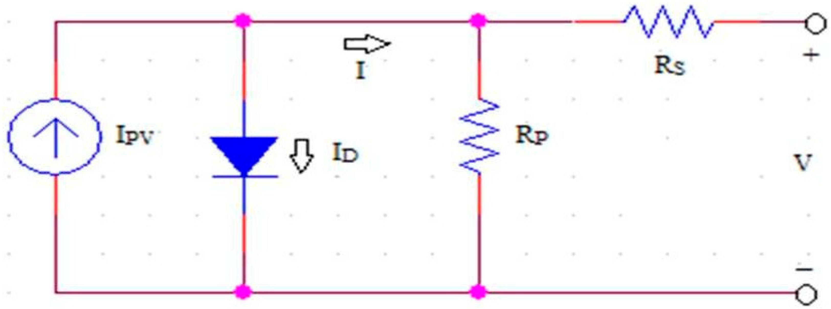
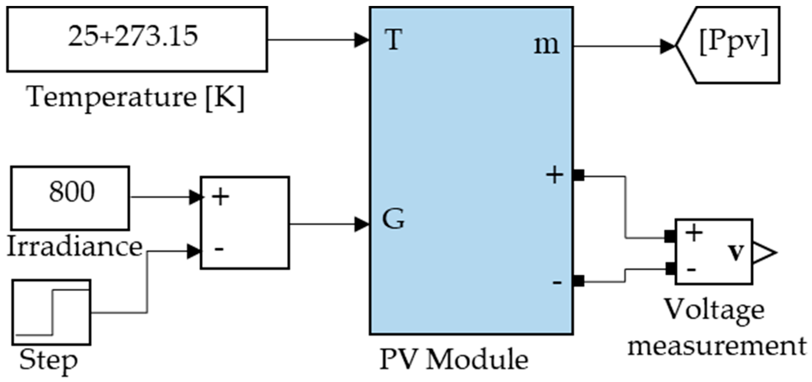
2.1. Modelling of the Solar PV System

The modeling of a PV cell includes a p-n diode of a semiconductor device that efficiently converts sun energy into DC current using PV effects. A sizeable number of PV cubicles are coupled in series and parallel arrangements corresponding to energy requisites. This alignment resultingly forms a PV module. However, the combination of various PV modules interconnected in a series improves the reliability of increasing the voltage level of the array, and parallel connections effects reasonably intensify the current in the array as well [2,11,20]. The corresponding circuit model of a PV cell encompasses a current source of (${\mathrm{I}}_{\mathrm{P}\mathrm{V}}$) connected in parallel with a reversed diode (${\mathrm{I}}_{\mathrm{D}}$), a parallel shunt resistor (${\mathrm{R}}_{\mathrm{p}}$), and a series resistor (${\mathrm{R}}_{\mathrm{S}}$), as depicted in Figure 2 [13,21].

A shunt resistor (${\mathrm{R}}_{\mathrm{P}}$) characterizes the leakage current of diode and series resistance (${\mathrm{R}}_{\mathrm{S}}$), which exemplifies inner losses as a consequence of current flow. The achievement of PV cells is contingent on two main elements, i.e., temperature and solar luminance. The following Equations (1)–(4) represent the behaviors of PV devices [18,22]:

$$\mathrm{I}={\mathrm{I}}_{\mathrm{P}\mathrm{V}}-{\mathrm{I}}_{\mathrm{D}}$$

(1)

where

$${\mathrm{I}}_{\mathrm{D}}=I_0[\mathit{exp}\left[\frac{\mathrm{q}\ast \mathrm{v}}{\mathrm{a}\ast \mathrm{k}\ast \mathrm{t}}\right]-1]$$

(2)

So,

$$\mathrm{I}=I_{pv}-I_0[\mathit{exp}\left[\frac{\mathrm{q}\ast v}{\mathrm{a}\ast \mathrm{k}\ast t}\right]-1]$$

(3)

$$\mathrm{I}=I_{pv}-I_0\left[\mathit{exp}\left[\frac{V+{\mathrm{R}}_{\mathrm{s}}}{a\ast V_t}\right]\right]-\left[\frac{\mathrm{V}+{1\mathrm{R}}_{\mathrm{s}}}{{\mathrm{R}}_{\mathrm{p}}}\right]$$

(4)

where, in the above equations, “I” indicates the solar cell current (A), $I_{pv}$ presents the current created by the light incident (A), ${\mathrm{I}}_{\mathrm{D}}$ represents diode current, q is the charge on electron, and “K” indicates the Boltzmann constant. T[K] represents the temperature of P-N junction. “a” is the diode constant, $V_t$ indicates the thermal voltage of array, ${\mathrm{R}}_{\mathrm{s}}$ is the equivalent resistance in the series connection, ${\mathrm{R}}_{\mathrm{p}}$ highlights the parallel connected resistance, and $I_0$ shows the diode saturation current (A).

The complete system schematic depicted in Figure 1 has been modeled in Simulink, MATLAB R2012a. Various modules of the proposed PV system are discussed in the subsequent sections. The solar PV module connected with irradiance, temperature, and panel voltage measurements is shown in Figure 3, where temperature (T) and solar irradiation (G) are the inputs of solar PV panels [18,22]. To make the nature of the PV panel generic, it is necessary to create a mask of the module for user inputs. The mask created for this purpose is shown in

Table 1. The studied generalized PV module mask.

System Parameters	Values
No of cells in series (${\mathrm{N}}_{\mathrm{S}}$)	10
No of cells in series (${\mathrm{N}}_{\mathrm{P}\mathrm{P}}$)	10
Diode constant (a)	1.3
Boltzmann constant (K)	1.38 × 10−23
Short-circuit current/temp coefficient (${\mathrm{K}}_{\mathrm{I}}$)	0.0032
Nominal temperature (${\mathrm{T}}_{\mathrm{n}}$)	298.15
Nominal irradiance (${\mathrm{G}}_{\mathrm{n}}$)	1000
Electron charge (q)	1.602 × 10−19
Nominal current (${\mathrm{I}}_{\mathrm{p}\mathrm{v}\mathrm{n}}$)	3.8
Nominal voltage of open circuit (${\mathrm{V}}_{\mathrm{o}\mathrm{c}\mathrm{n}}$)	42.1
Open-circuit voltage/temp coefficient (${\mathrm{K}}_{\mathrm{v}}$)	−0.123
Nominal short-circuit current (${\mathrm{I}}_{\mathrm{S}\mathrm{c}\mathrm{n}}$)	3.8
Series resistance (${\mathrm{R}}_{\mathrm{S}}$)	0.473
Parallel resistance (${\mathrm{R}}_{\mathrm{P}}$)	1367

. The parameter influences on the performance of the PV module depend on the following: where ${\mathrm{N}}_{\mathrm{S}}$ represents the number of cells in series arrangement, ${\mathrm{N}}_{\mathrm{p}\mathrm{p}}$ indicates the number of parallel connected modules, and ${\mathrm{N}}_{\mathrm{S}\mathrm{S}}$ represents the series-connected module numbers. Further, a diode constant “a” is 1.3977, ${\mathrm{I}}_{\mathrm{s}\mathrm{c}\mathrm{n}}$ is the short-circuit nominal current, ${\mathrm{K}}_{\mathrm{p}}$ indicates the short-circuit voltage/temperature constant, ${\mathrm{K}}_{\mathrm{I}}$ represents the current/temperature coefficient, ${\mathrm{V}}_{\mathrm{m}\mathrm{p}}$ represents the maximum voltage power at STC, and ${\mathrm{I}}_{\mathrm{m}\mathrm{p}}$ is the current at the maximum power at STC of generalized PV systems. Additionally, the mask shown in

Table 2. The switching state illustration of three-phase inverter.

States	ON Switches	Van	Vbn	Vcn	Space Voltage Vectors
0	462	0	0	0	V0 (000)
1	162	2(VDC/3)	−(VDC/3)	−(VDC/3)	V1 (100)
2	132	(VDC/3)	(VDC/3)	−2(VDC/3)	V2 (110)
3	432	−(VDC/3)	2(VDC/3)	−(VDC/3)	V3 (010)
4	435	−2(VDC/3)	(VDC/3)	(VDC/3)	V4 (011)
5	465	−(VDC/3)	−(VDC/3)	2(VDC/3)	V5 (001)
6	165	(VDC/3)	−2(VDC/3)	(VDC/3)	V6 (101)
7	135	0	0	0	V7 (111)

demonstrates the parameters for the BP MSX 120 array PV model; parameters are taken from its datasheet [18,23]. However, modifying these parameters for any additional PV panel is possible.

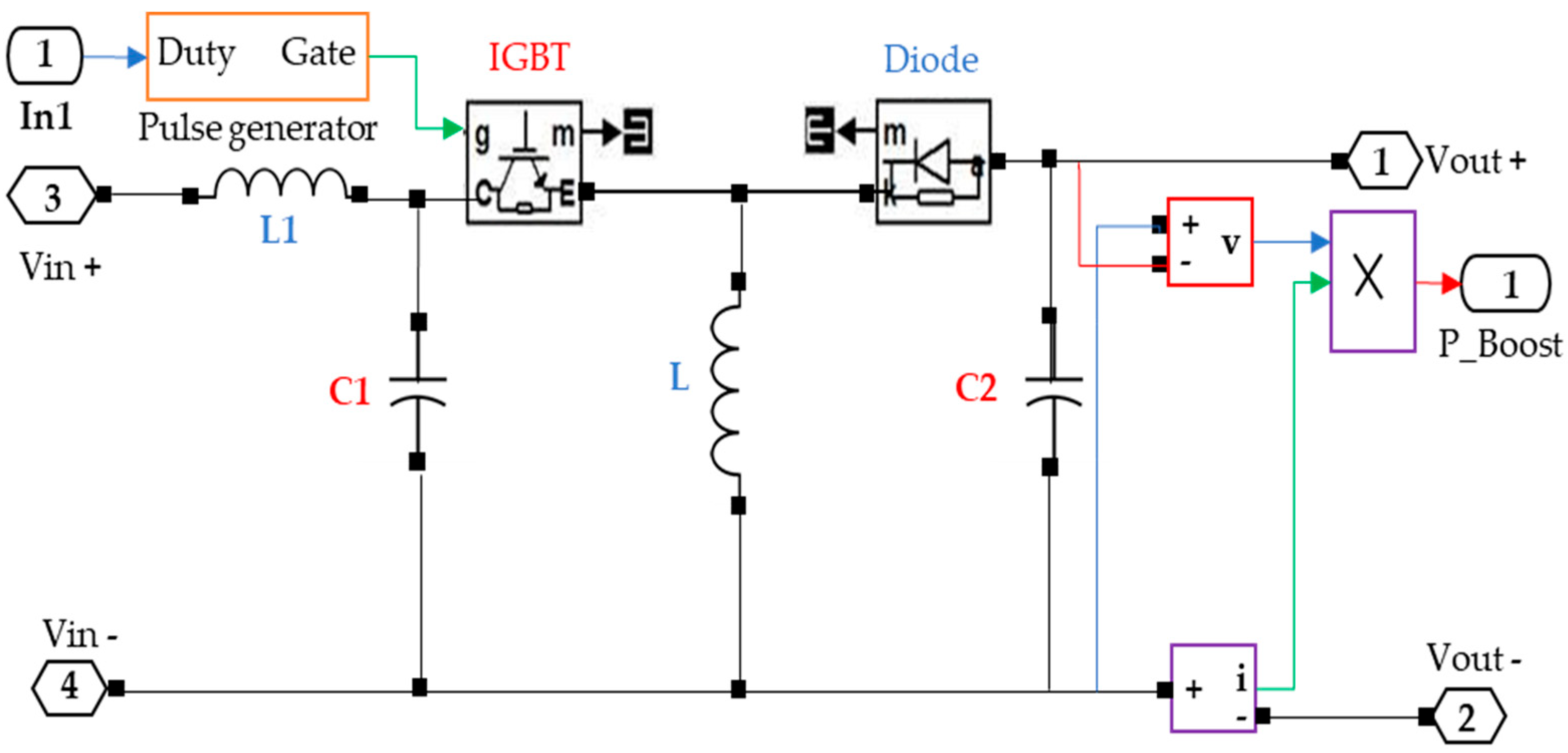
2.2. DC/DC Boost Converter

The primary function of the PV-connected DC/DC boost converter is to momentarily store input power from the solar panel and then deliver it by discharging the energy to the connected load side, ensuring that distinctive levels of maximum power have been transferred in the form of voltage and current [24]. A non-reversing buck–boost converter is, in effect, a tumbled arrangement of a buck converter tailed by the operating boost converter in the system. This study applied a single inductor and capacitors, which are adopted efficiently to implement both converters. The adopted power converters utilize two active switches designed by cascading buck and boost converters. This generates a minimal or elevated output voltage compared to the input voltage due to the buck–boost nature of the power converters used in the energy sector [18]. In this paper, a boost converter studied in [25,26,27] has been implemented, as shown in Figure 4.

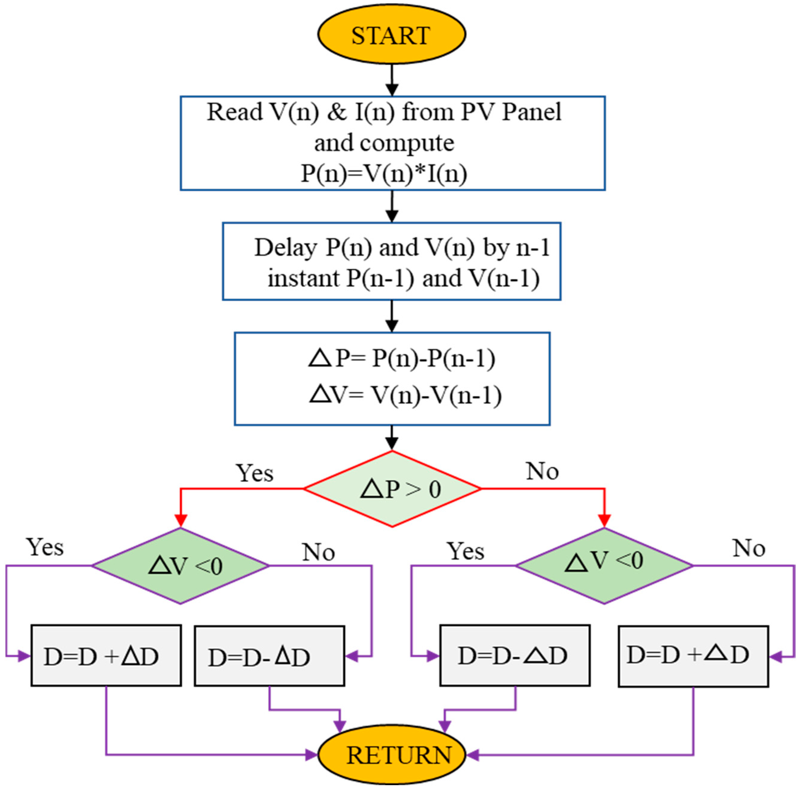
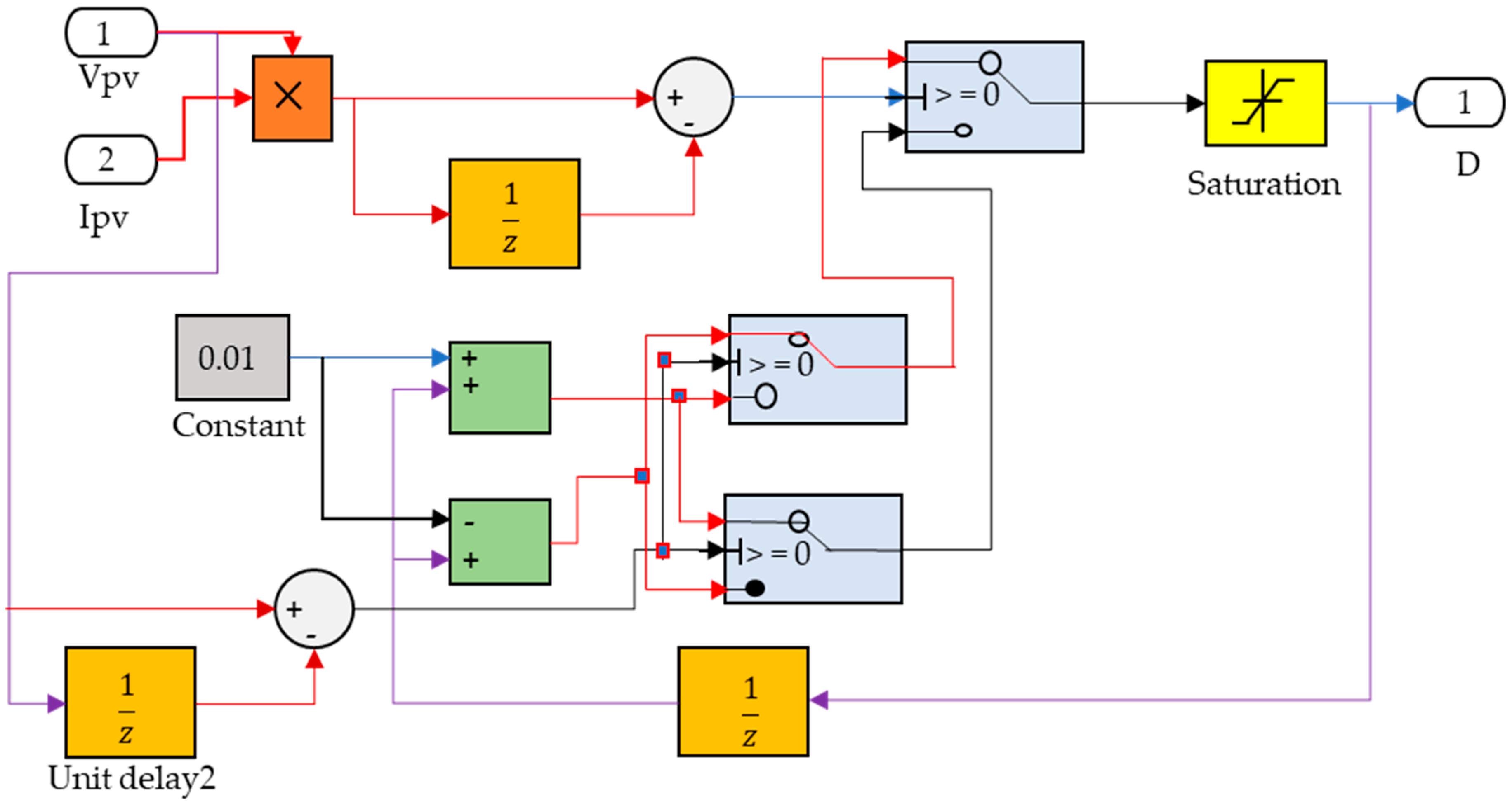
2.3. MPPT Control Algorithm

The PV system’s power generation typically depends on various environmental conditions, such as temperature and solar irradiance. However, solar PV systems’ minimum efficacy and cost effectivity demand that the PV system be operated at a maximum power point (MPP). The MPP of a solar PV system varies according to the varying atmospheric conditions or load fluctuations in the PV-connected system. The typical PV panel converts about 30–40% of instance solar radiation into electrical energy to operate stably [28]. For this purpose, different MPPT control algorithms have been cultivated and instigated to upsurge/improve the operational efficiency of PV systems. Moreover, the non-linear output features of the PV model are effectively altered with variations in solar irradiance and the cell temperature.

Furthermore, uncertain behaviors of solar irradiation affect the MPP of the designed PV module. Thus, a robust MPPT control algorithm becomes vital to the function of the PV module in its MPP operation. To overcome this issue, various MPPT controllers are adopted; however, the most prevalent approaches are studied using the P&O algorithm. Further, machine-learning-based artificial neural network techniques for MPPT control have been studied for PV systems. In [17,29], the authors presented a fuzzy-logic-based controller and incremental conductance method presented for the MPPT of solar PV modules [30,31].

This paper presents the most frequently used P&O MPPT algorithm for a generalized PV system based on a laid-back execution process and requiring less economic factors. The studied P&O algorithm efficiently operates by adjusting the operating voltage of the PV array and examining the PV output power more quickly. The algorithm functions as the power varies with the variation in voltage when moving towards the right of the MPP. Additionally, when moving on the right of the MPP, the variation in power increases with the variation in voltage relations.

Consequently, if the system detects rises in power, the sequential perturbation maintains the identical value to obtain the MPP, the increase (decrease) in power increases with the decrease (increase) in voltage relations. Consequently, if the system detects rises in power, the sequential perturbation maintains the identical value to obtain the MPP. Similarly, if there is a drop in power, the perturbation operates in reverse. The flowchart of the studied P&O algorithm for an MPPT of a generalized PV module is depicted in Figure 5. However, this implemented algorithms must involve two key measurements, i.e., voltage ($V_{PV}$) and current ($I_{PV}$) [13]. The MPPT model implemented in this study is depicted in Figure 6.

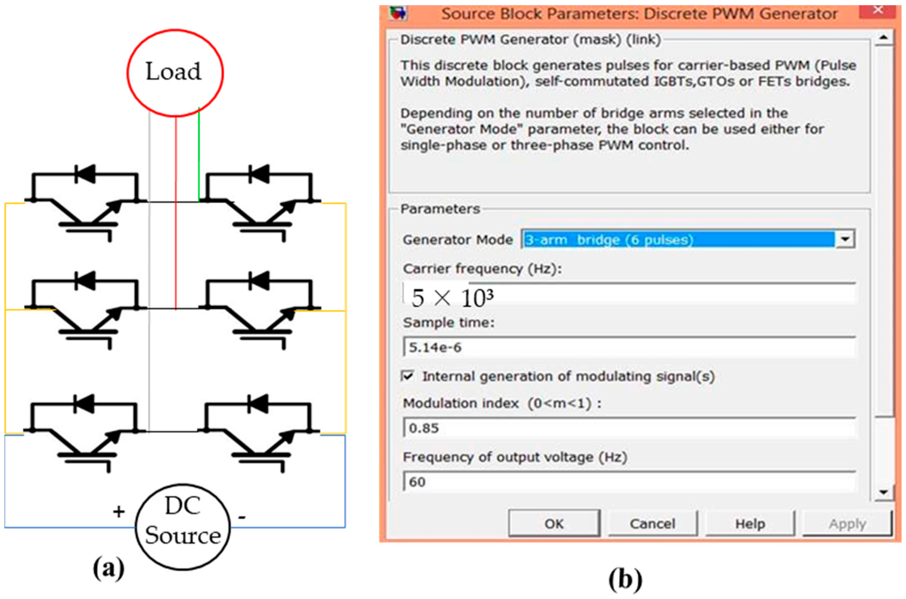
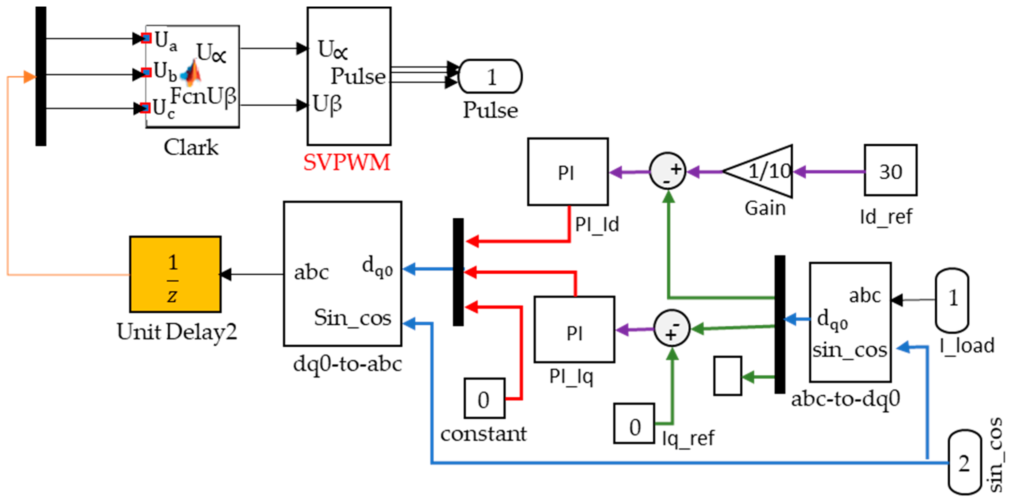
2.4. The DC/AC Power Inverter

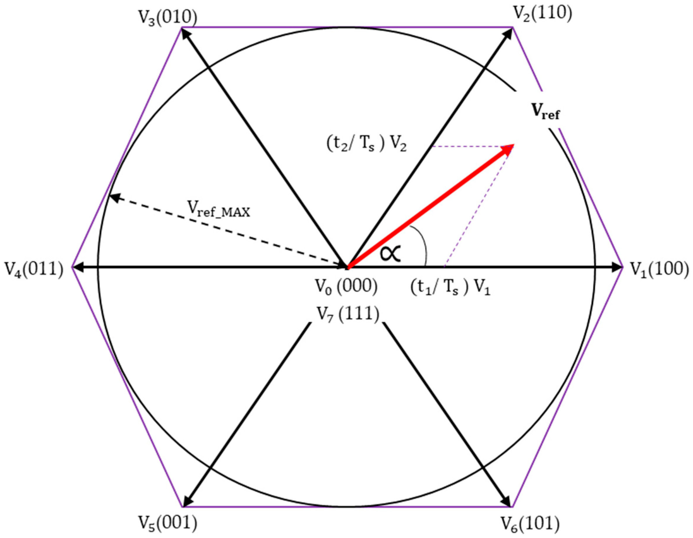
It is an electronic device that transforms the DC power to AC [1,5]. AC power can be obtained at any rating; AC power is adjusted by its frequency using suitable transistor switching, by gates or through timers via generating clock signals. For stepping down or stepping up the voltage to the required level, transformer rating is used. Figure 7a shows the Simulink model for the three-phase inverter. As it is a three-phase inverter, six ideal switches were used. To generate the pulse width modulation (PWM) signal of the inverter, the pulse generator block from Simulink was used. Figure 7b shows the internal values for the pulse generator that were used.

SVPWM Technique

Space vector modulation (SVM) is the modulation technique that was established as a vector approach to PWM signal generators. It was developed to be used in three-phase inverters as a feedback controller. This technique generates a pure sinusoidal sine waveform that has a lower total harmonic distortion (THD) and produces high voltage. This quality makes it the best to use in power electronics. The main objective of the SVPWM modulation approach is to obtain maximum variable output with minimum harmonics [32]. In the context of the deep learning technique, consider a three-phase half-bridge voltage source inverter [33], three voltages, each phase to the center-tap voltages can have only two possible values, namely +${\mathrm{V}}_{\mathrm{d}\mathrm{c}}$/2 or −${\mathrm{V}}_{\mathrm{d}\mathrm{c}}$/2, respectively. The three IGBT switches correspond to three phases, so at any time instant the inverter has eight possible states. If the upper switch of the leg is on, it is indicated by state 1. Similarly, if the lower switch of a particular leg is on, it is indicated by state 0. As there are three legs, there are eight possible switching combinations. The line to neutral voltages can be found using the following three equations:

$$V_{an}=[2V_{ao}-V_{co}-V_{bo}]/3$$

(5)

$$V_{bn}=[2V_{bo}-V_{ao}-V_{co}]/3$$

(6)

$$V_{cn}=[2V_{co}-V_{ao}-V_{bo}]/3$$

(7)

The summary of these states and lines to the neutral voltage applied accordingly is shown in Table 2, studied by [5,8,33].

So, there are six active states of the inverter and the remaining two are zero states. The line to neutral voltages, i.e., $V_{an}$, $V_{bn}$, and $V_{cn}$, are 120° apart. Two phase equivalents of the line to neutral voltages are written as follows:

$$V_{ref}=V_{ds}+\mathrm{j}{V}_{qs}$$

(8)

By using Clark’s transformation, the values of $V_{ds}$ and $V_{qs}$ are obtained. From Equation (8), the magnitude and phase of the voltage $V_{ref}$ can be determined. When plotting the magnitude and phase, the space vector magnitude and position corresponding to each switching state are determined as shown in Figure 8. Each of the vectors, such as V100, V110, etc., shown in the diagram represent six voltage steps developed by the inverter with zero voltages, V000 and V111, located at origin. The inverter switches are in a steady state at each of these states. A switching pattern must be devised that produces a voltage which transitions in between these states, and not only at the six vector states, in order to develop a sine wave at the motor. This effectively produces a continuous rotating vector $V_{ref}$, which transitions smoothly from state to state.

A vector is produced that transitions smoothly between sectors using the appropriate PWM signals, and hence provides sinusoidal line to line voltages which are equivalent to the input reference voltage. Thus, by using the space vector modulation technique, the output voltages of the inverter are almost equal to the input reference voltages. The reference voltage is sampled at a particular frequency to obtain such output voltages. The output voltage will be closer to the reference voltage if the sampling frequency is greater, but as the sampling frequency increases, the switching frequency also increases, which further results in increased switching loss. So, an optimum sampling frequency should be selected to overcome this problem. A formula must be derived to obtain the PWM time intervals for each sector. By sampling the reference voltages, the time in which active vectors are switched and the sector in which these vectors are switched are obtained. The time and sector can be found from the magnitude and the position of reference voltages. The symbols T1 and T2, respectively, represent the time periods in which the active vector along the lagging edge and the leading edge are switched in order to understand the reference voltage space vector in a given sampling period. Ts is the symbol that represents the sampling time period. The times T1 and T2 can be obtained by applying volt-sec balance in vector form. The volt-sec balance along the $d_s$ and $q_s$ axis is written as follows from Equation (8):

V_ref ∗ T_s ∗ cos(α) = [(V1 ∗ T1 ∗ cos(0)) + (V2 ∗ T2 ∗ cos(60))]

(9)

V_ref ∗ T_s ∗ sin(α) = [(V1 ∗ T1 ∗ sin(0)) + (V2 ∗ T2 ∗ sin(60))]

(10)

where $V_s$ is the magnitude of the reference voltage and V1 and V2 are the magnitudes of the sector voltages that are equal to the DC link voltage, $V_{dc}$. The “α” is the position of the reference vector in accordance with the beginning of the sector, where the reference vector’s tip lies. Rearranging Equations (8) and (9), the switching time T1 and T2 are found and is stated as follows:

T1 = {[V_s ∗ T_s ∗ sin(60 − α)]/(V_dc ∗ sin(60))}

(11)

T2 = {[V_s ∗ T_s ∗ sinα]/(V_dc ∗ sin(60))}

(12)

The sampling time is as follows:

T_s = (T1 + T2 + T0)

(13)

In Equation (13), T0 is the time at which the null vectors (0 and 7) are switched on.

2.5. The Inverter Connected to Grid

For grid-connected systems, it is important to synchronize the inverter’s voltage and frequency with the grid. For this purpose, synchronization between the inverter and the grid was performed via a feedback system. A built-in SIMULINK PLL block was used. The purpose of the PLL block is to generate the grid’s frequency, voltages, and phase angle, which are then fed into the SVPWM block. The SVPWM block generates a signal for the inverter, hence the output is synchronized with the grid. The SVPWM block was designed based on the model presented in [11,26]. The model under a mask of the SVPWM block is shown in Figure 9. The inputs of this block are the output from the PLL block and the current from the inverter. It generates the switching signal that is again fed to the inverter. This is how this model for the feedback system works in grid-connected mode.

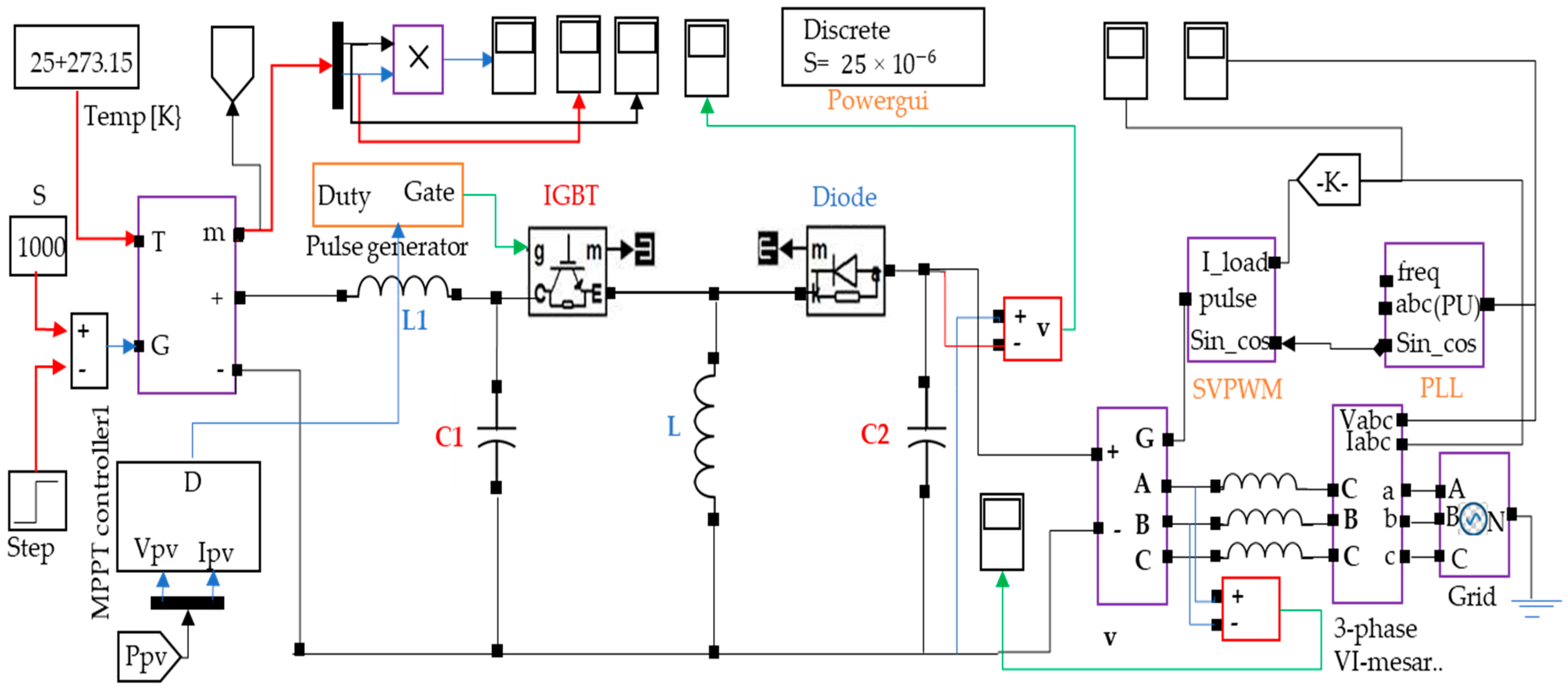
3. The Studied System Simulation Model

The model simulations of the PV array connected with the boost converter and the synchronization of the inverter with the grid performed efficiently. Moreover, the presented system successfully performs operations with any PV array model by consigning the specific parameters in the mask illustrated in Figure 4. This study adopted the BP MSX 120 PV model for simulation. The proposed system as a whole Simulink implementation is depicted in Figure 10. Moreover, the temperature, irradiance, and connected load were fluctuated during system operation to evaluate the potential of the MPPT controller to track the MPP under sudden variations in environmental conditions and unpredictable load.

4. Simulation Results and Discussion

Table 3. The test system parameters of studied BP MSX 120 PV system.

BP MSX 120 (Components)	System Values and SI Units
Short-circuit current	3.56 (A)
Current at MPP	3.87 (A)
Voltage at MPP	33.7 (V)
Open circuit voltage	42.1 (V)
Number of cells in series	72

demonstrates the key attributes of the BP MSX 120 PV model at an STC of about 25 °C [17]. In addition, to design the generalized PV array model BP MSX 120, modules were interconnected in series or in parallel arrangement. In this study, the 12 KW PV array module was developed through the connection of ten modules in both series and parallel arrangements to perform the MPPT control operation. The primary features of this array module to perform stable operation are already illustrated in Figure 3.

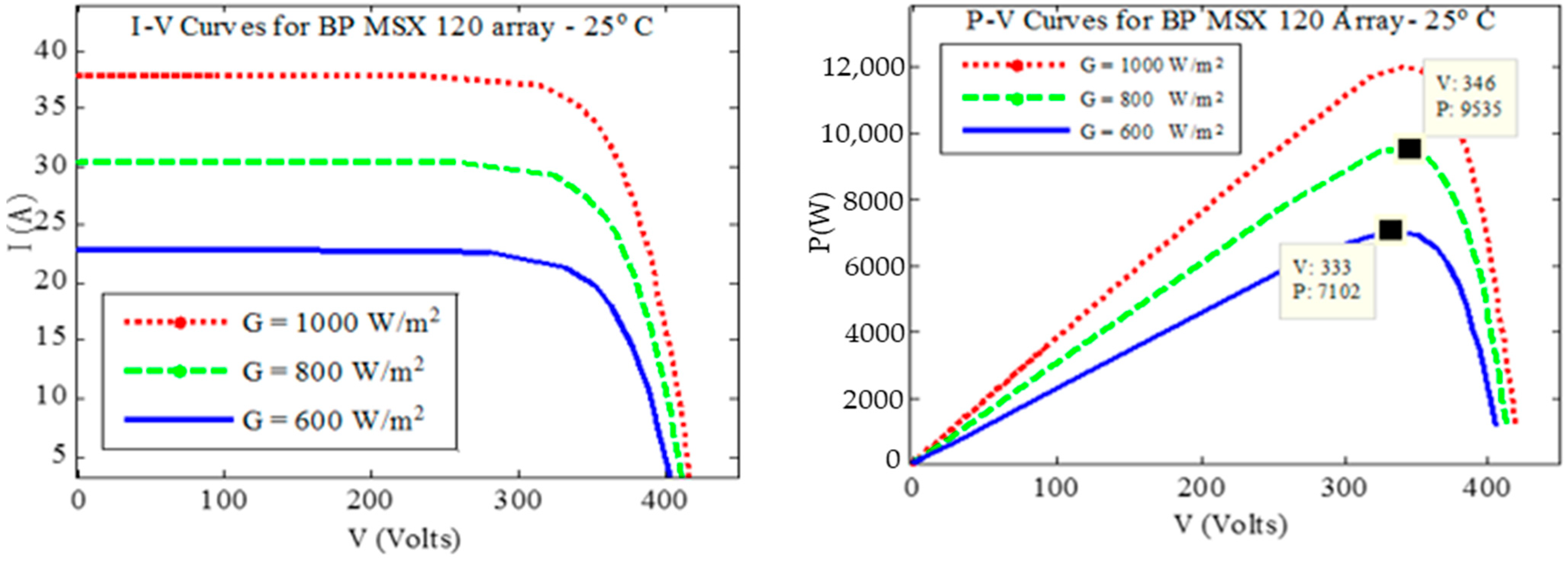
4.1. The PV Array Features under Erratic Temperature and Radiation

In the studied system, the primary features of the PV array model as a function of varying temperature (T) and solar irradiance (G) provide the relational characteristics curves of the power–voltage (P-V) and voltage–current (V-I) relations, as presented in Figure 11 and Figure 12. These curvatures, i.e., P-V and I-V, are significantly non-linear and dependent on system temperature and solar irradiation. Moreover, under different values of irradiance (G), the obtained P-V and I-V characteristic curves in the studied system are depicted in Figure 12. From the figure, the direct relation between irradiance and the current features can potentially be observed. By increasing the solar irradiation, the current also increases, which is slightly higher in comparison with the voltage level and maximizes the MPP features as well. Figure 11 illustrates that the P (W) to V (Volts) and I (A) to V (Volts) feature curvatures of the studied PV array model with different values of temperature in the system. From the figure, it is logical to conclude that increasing the temperature results in a reduction in the power and PV array voltage level; however, the system’s current remains constant. Thus, the variation in temperature shows zero effect on the current features.

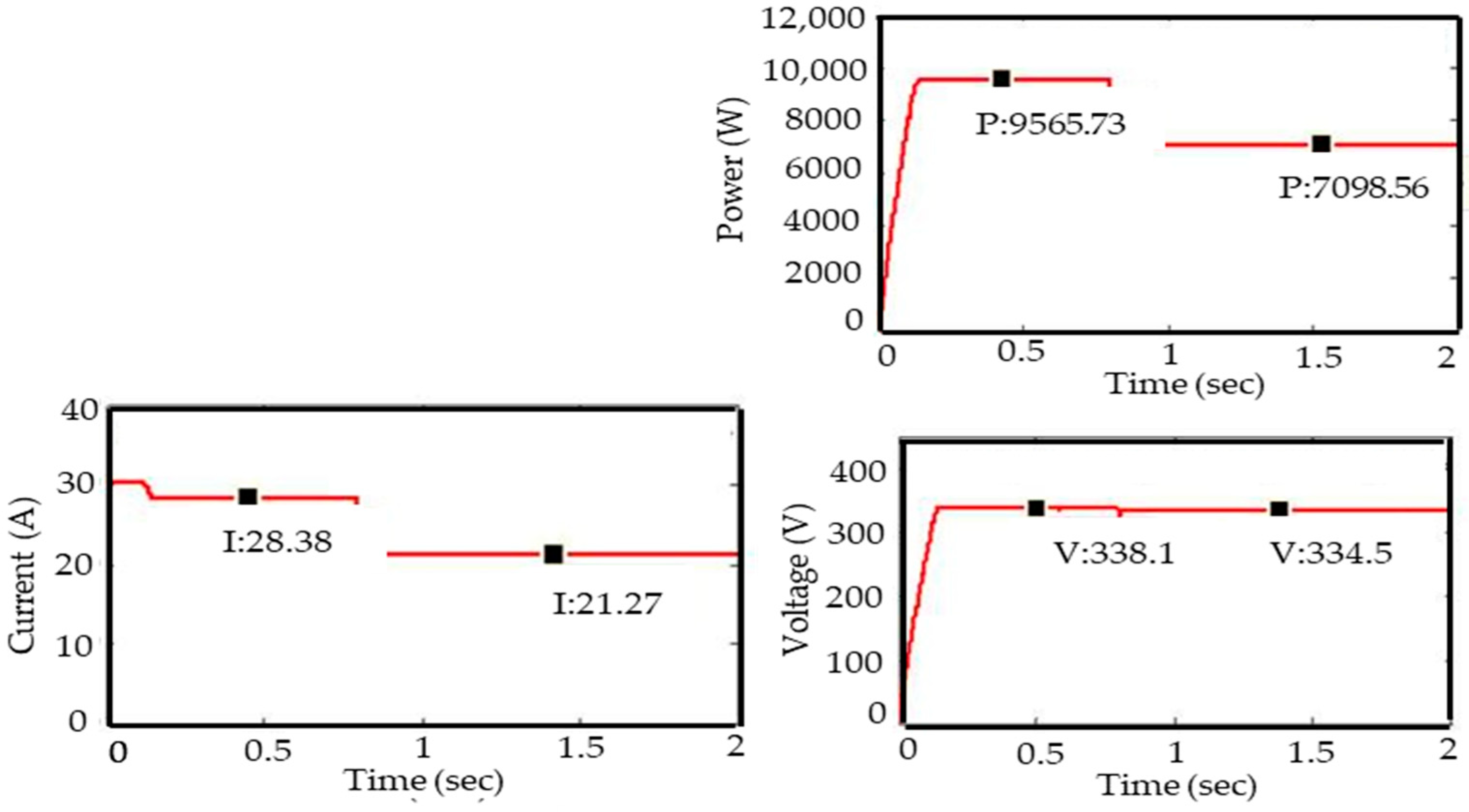
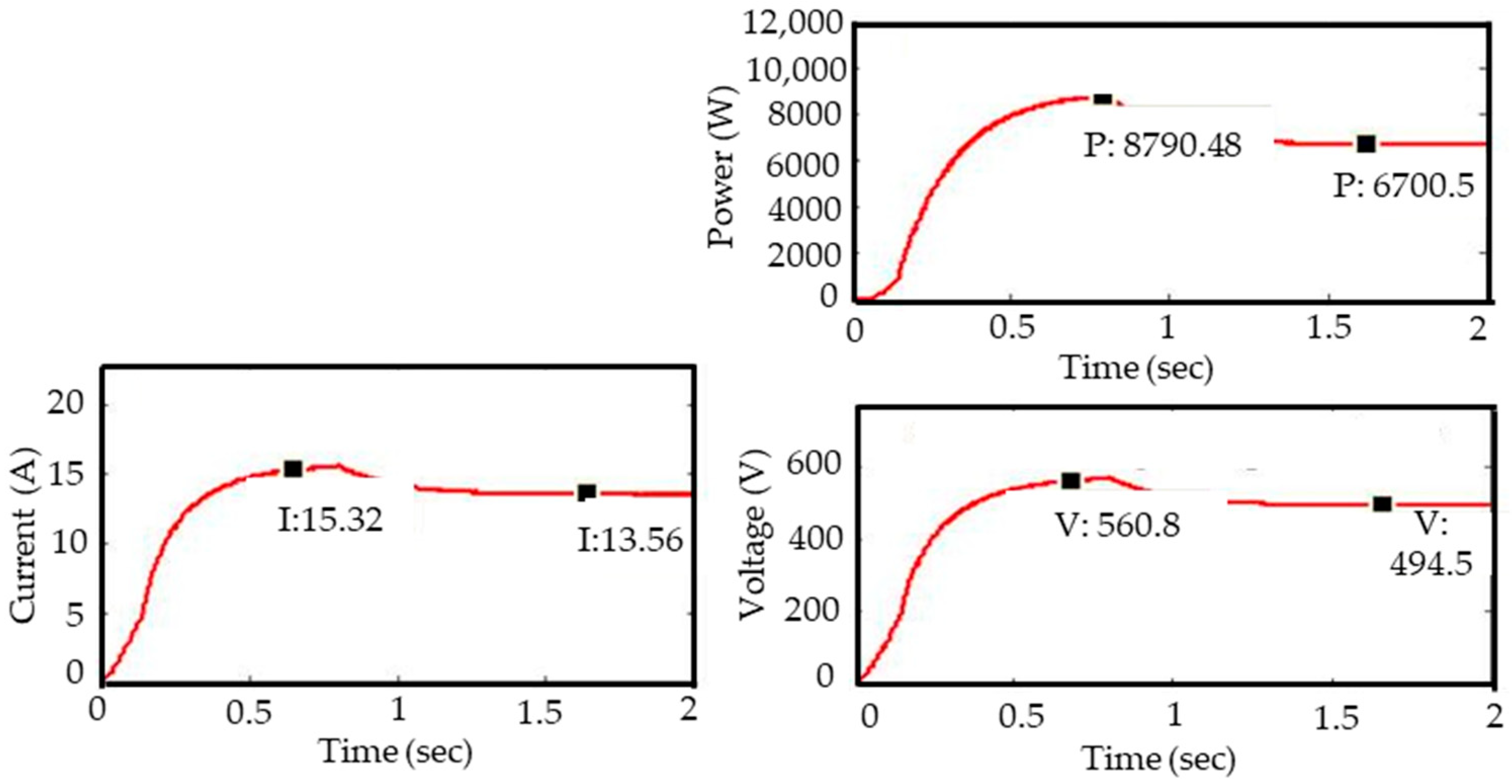
4.2. The PV System Performance during Hasty Solar Radiation (G) Variance

The performance of the PV system during sudden variations in solar irradiance (G), temperature (T), and fluctuating load was examined to scrutinize the effectiveness of the proposed system under MATLAB/simulation. For this purpose, the analysis of the presented system was carried out by step variation in irradiation (G) and by holding the cell temperature constant at about 25 °C. Initially, the solar irradiation (G) value set was 800 [W$/{\mathrm{m}}^2$] during the operation, then at a time (t = 1 s) a sudden change in irradiation to 600 [W$/{\mathrm{m}}^2$] was applied. The effects of abrupt variations in radiation (G) on the PV system’s output power (P), voltage (V), and current (I) are presented in Figure 13. The obtained result illustrates that PV output power suddenly changes from 9566 W to 7098 W due to step fluctuations in irradiance (G). Moreover, PV voltage is independent of irradiance (G); thus, a gradual variation in irradiance presents practically zero effect on the system’s voltage value. From Figure 14, it can be observed that the output voltage of the PV system fluctuates near the maximum power following the applied P&O control algorithm. However, an abrupt variation in solar irradiance (G) from 800 to 600 [W$/{\mathrm{m}}^2$] affects the current value of the PV system, and a resulting reduction in the current value from about 28.5 A to 21.3 A is observed. The obtained results are identical to the features curves of the PV array model result presented in Figure 11 and Figure 12, respectively. The obtained result effectively authenticates the MPP operation of the studied PV scheme during sudden fluctuations in solar radiation (G). Moreover, a similar simulation was conducted to investigate the connected boost converter performance. The output voltage, current, and power of the system-connected boost converter are depicted in Figure 14. The presented results demonstrate that the boost converter’s output power is almost equal to the input power [11]. The adopted boost converter maximizes the voltage range from 338 to 560.8 V and minimizes the current values from 28.5 A to 15.32 A. Under step variation, the voltage decreases to 495 V, and the reduction in the current is found to be 13.6 A, which contributes to the approximate output power nearly identical to the input power. These obtained results demonstrate the capability of the boost converter to reach the MPP of the presented PV system during sudden variations in irradiation (G).

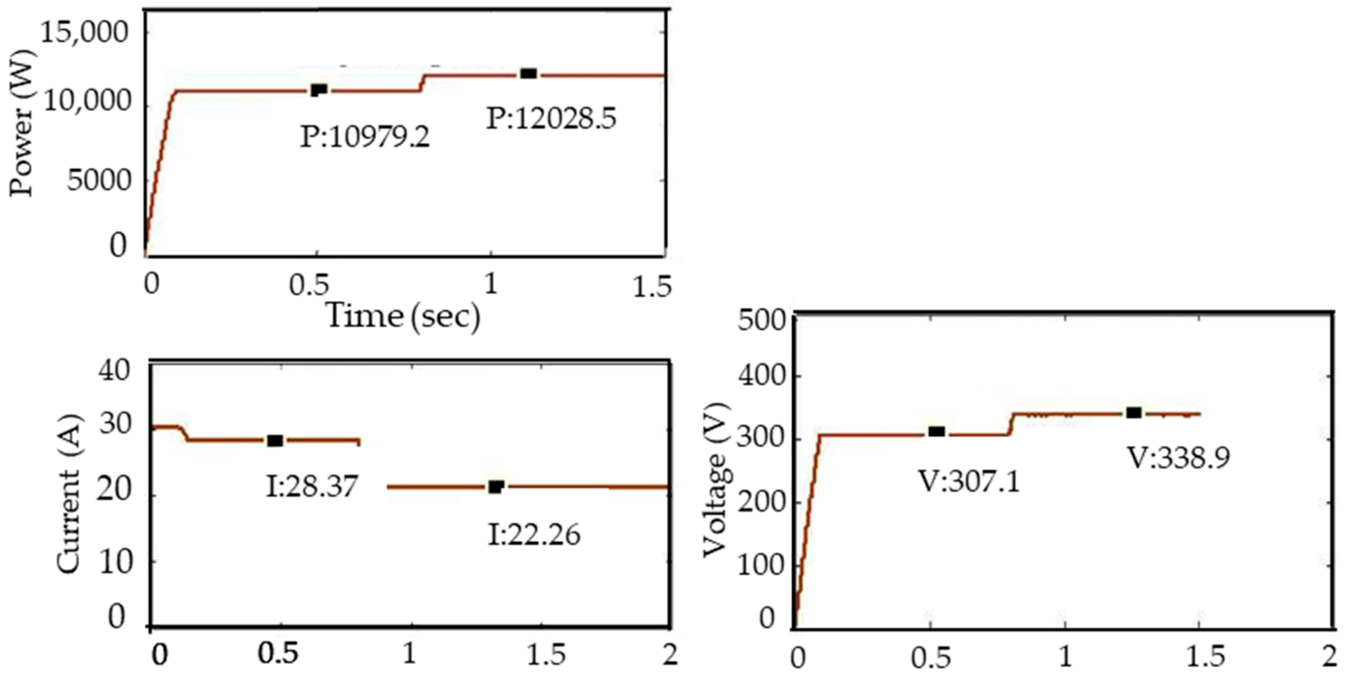
4.3. The PV System Performance during Sudden Variation in Temperature

The effectiveness of the studied PV system is obtained under sudden variations in temperature while maintaining solar irradiance. The simulation was carried out to analyze the performance of the PV system via changing the system temperature (T) from about 50 °C to 25 °C, while letting the solar irradiation (G) remain constant at G = 800 [W$/{\mathrm{m}}^2$]. During the execution, the process temperature of the system was fixed at 25 °C. However, at time t = 1 s, sudden variations in temperature happened from 50 °C to 25 °C under this situation; the subsequent output power (P), current (I), and voltage (V) of the adopted PV system are provided in Figure 15. From Figure 16, it can be observed that the PV output power increased in a range from 10,979.2 W to 12,028.5 W at system temperature variations of about 25 °C to 50 °C. This demonstrates that the presented PV system is operating at its MPP during the sudden variation in temperature. In addition, variation in temperature from 25 °C to 50 °C effectively maximizes the output voltage of the PV system from 307 V to 339 V. These obtained results are equivalent to the PV system feature graphs depicted in Figure 11 and Figure 12, which authenticates that the performance of the PV system under abrupt variations in temperature functions at the MPP of the system. Further, MATLAB/simulation was conducted to investigate the performance of the applied boost converter. The effect of temperature change on the boost converter’s output voltage, power, and current is illustrated in Figure 17. The boost converter enhances the voltage from 307 to 607 V, and a reduction in current is observed up to 28.4–16.64 A, while the output power remains identical to the input power as demonstrated in Figure 16; this significantly ensures the robust tracking of MPP by the studied boost converter.

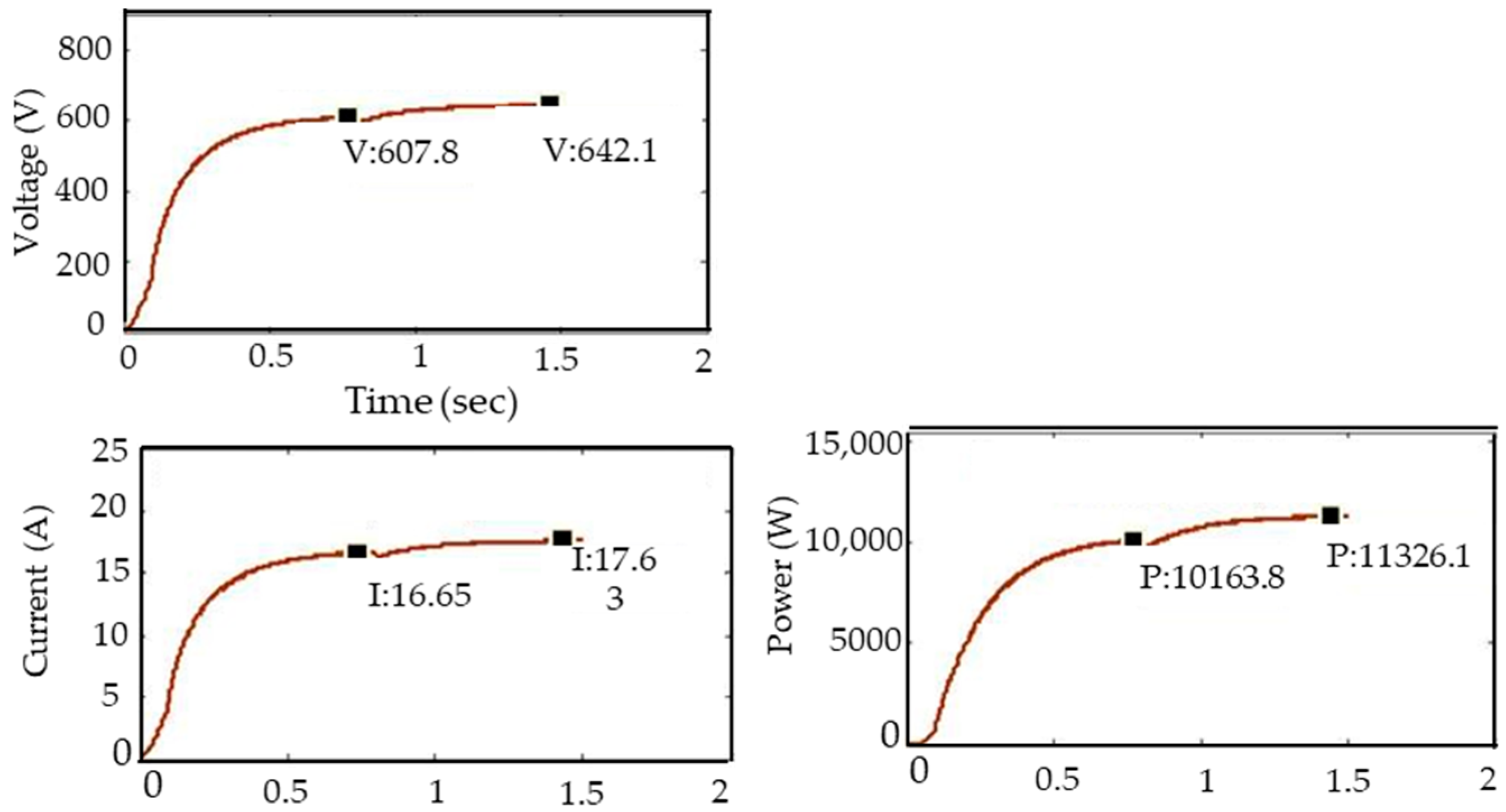
4.4. The PV System Performance with Variation in Load

The test simulation was carried out to analyze the PV array and the implemented MPPT control system’s performance during load fluctuation. During the execution phase, the resistant loads of 20 Ω were associated at the boost converter terminal. However, the temperature (T) and solar irradiation (G) of the PV system were fixed at about 25 °C and 800 (W$/{\mathrm{m}}^2$), respectively, resulting in PV output voltage, current, and power in relation to time, as presented in Figure 17. The results evidently revealed that the total output power obtained was about 12,029 W, the output current was about 35.72 A, and the voltage was about 340 V in the studied generalized PV system. Further, to identify the impact of load variation on the performance of the PV system, the load was maximized to double the initial load, i.e., 40 Ω connected with the system; however, the temperature and irradiance were kept constant during the double load events. Thus, with variable load, the output voltage, power, and current remain the same, reflecting the nearby zero effect of load variation on the studied PV system as depicted in Figure 18. The boost converter study cycle is varied to gain the maximum power and to deliver power to the connected load. The test result indicates the PV array provides the maximum voltage, power, and current self-regulation of load. The duty cycle can be regulated by using boost converters and MPPT control algorithms.

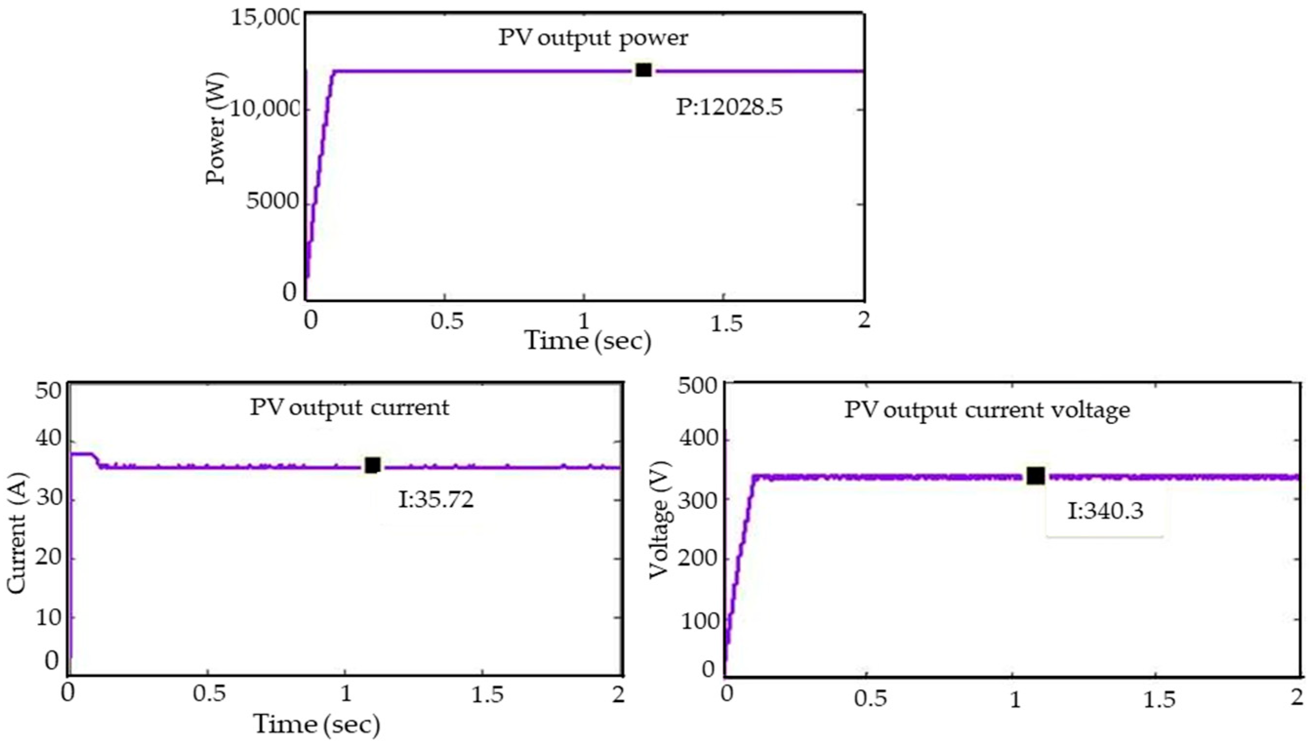
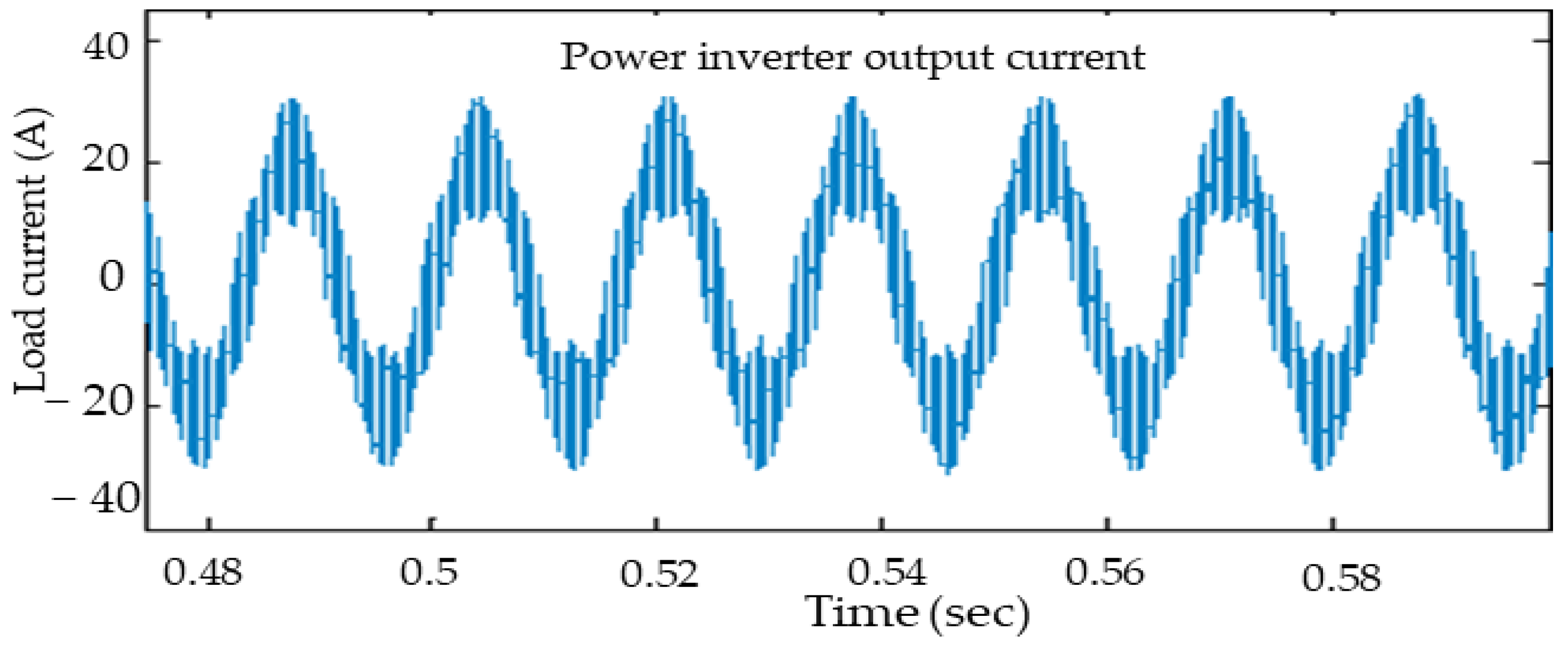
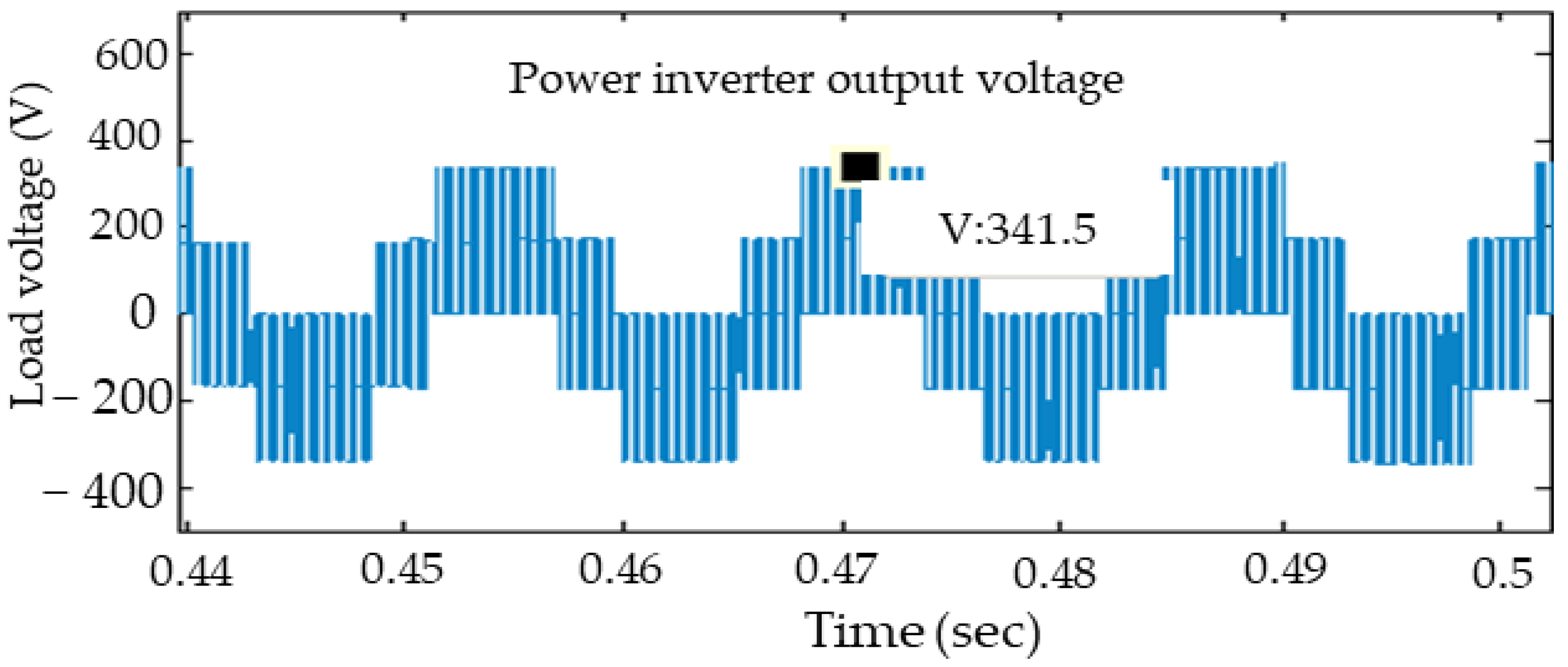
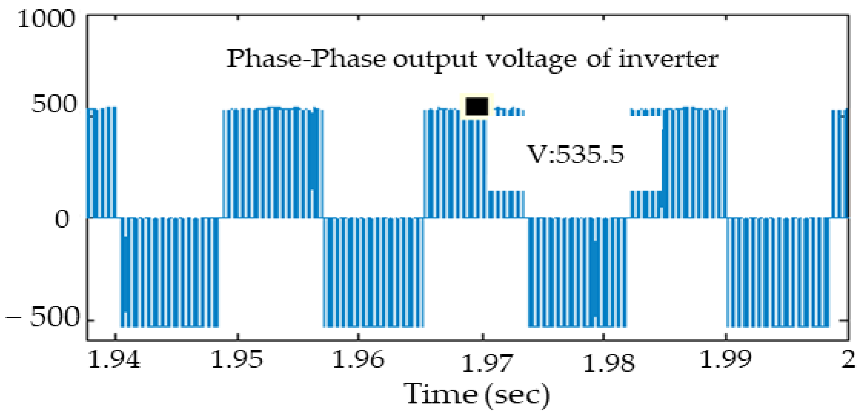
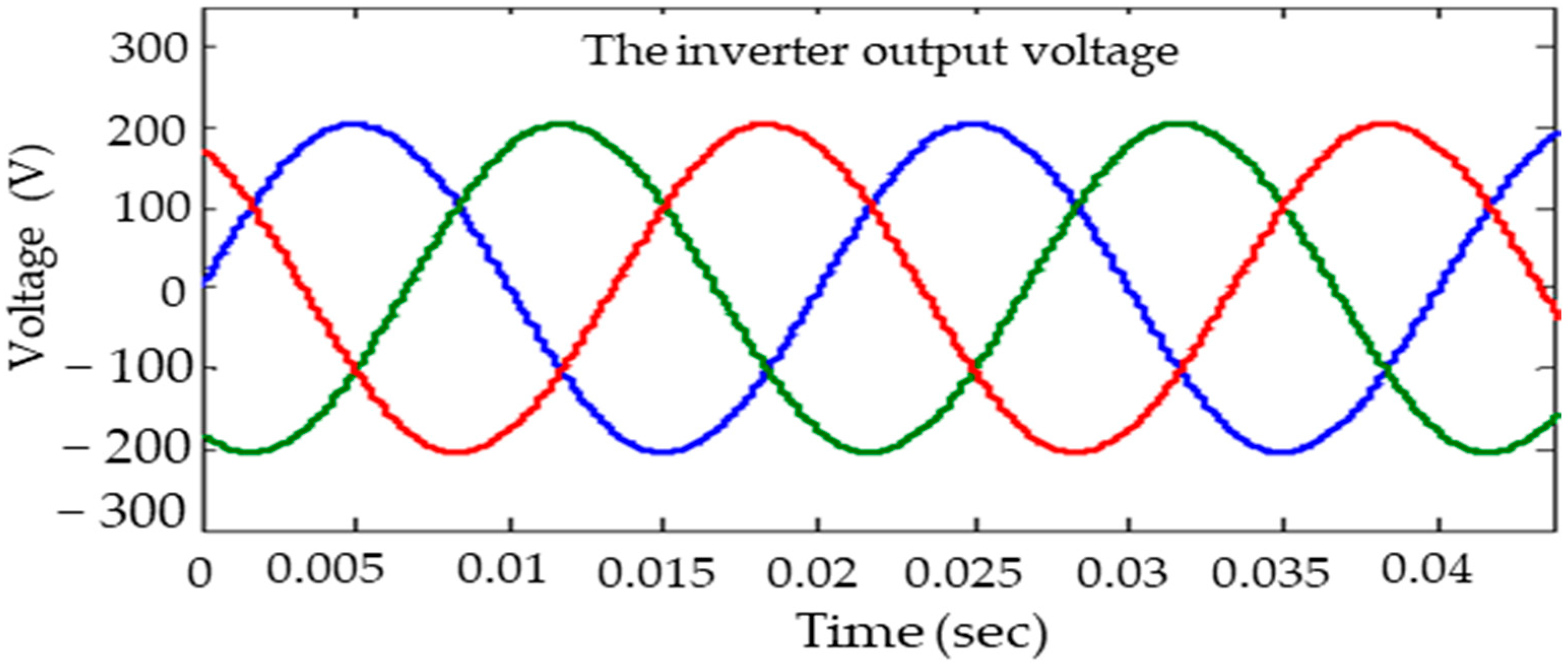
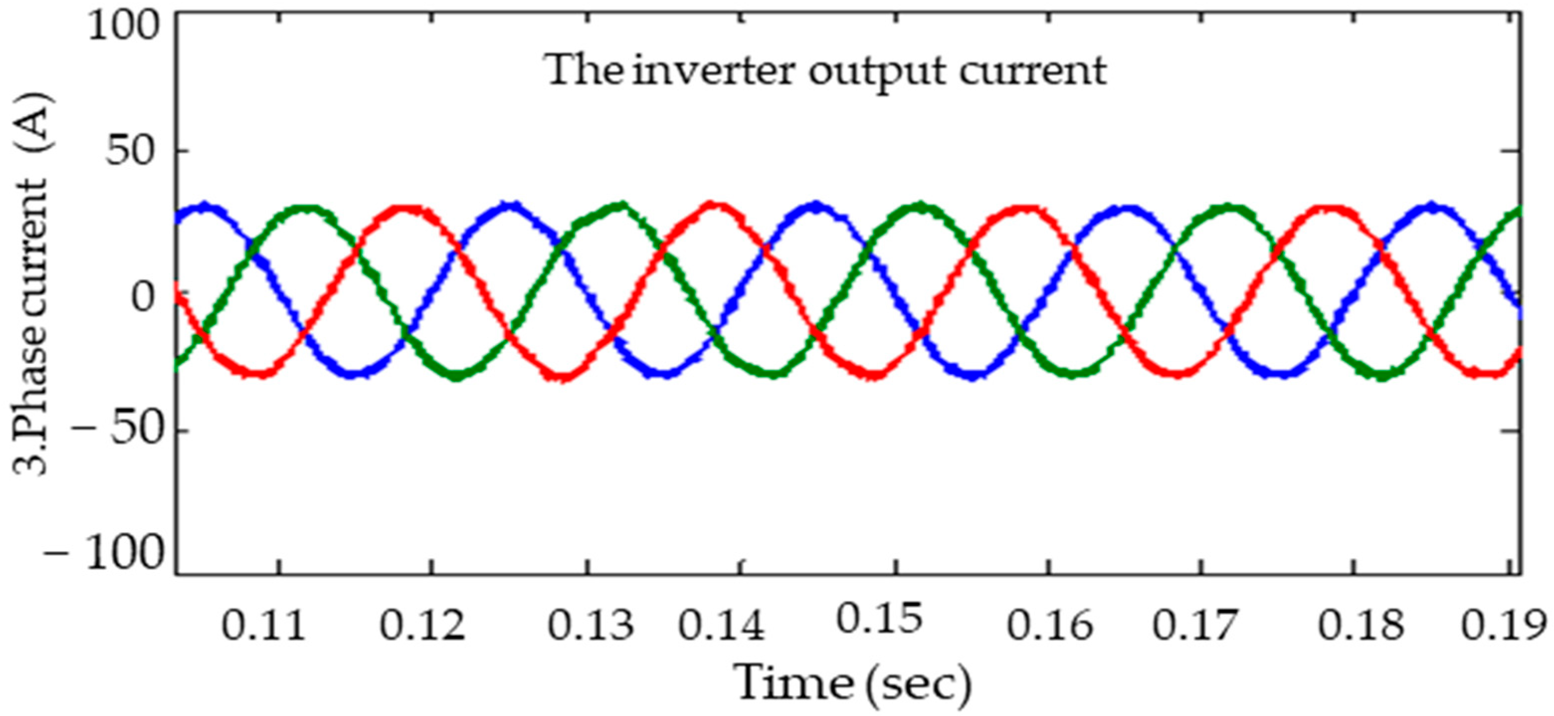
4.5. Three-Phase Inverter Connected to PV

The three-phase DC/AC inverter model is adopted to execute the designed PV system with 10 Ω of load connected with every single phase. However, the attribute of frequency carrier of 5 kHz and sampling time of about 5.14 × 10⁻⁶ s was created in the system following the study presented in [18]. The three-phase inverter operates to deliver a three-phase current to the connected load. A sinusoidal load current waveform for phase “a” is shown in Figure 19. Moreover, the PV system-generated DC voltage is converted to AC by the power inverter. Figure 20 and Figure 21 show the test system simulation outcomes of a three-phase power inverter output voltage regarding phase–ground and phase–phase, respectively.

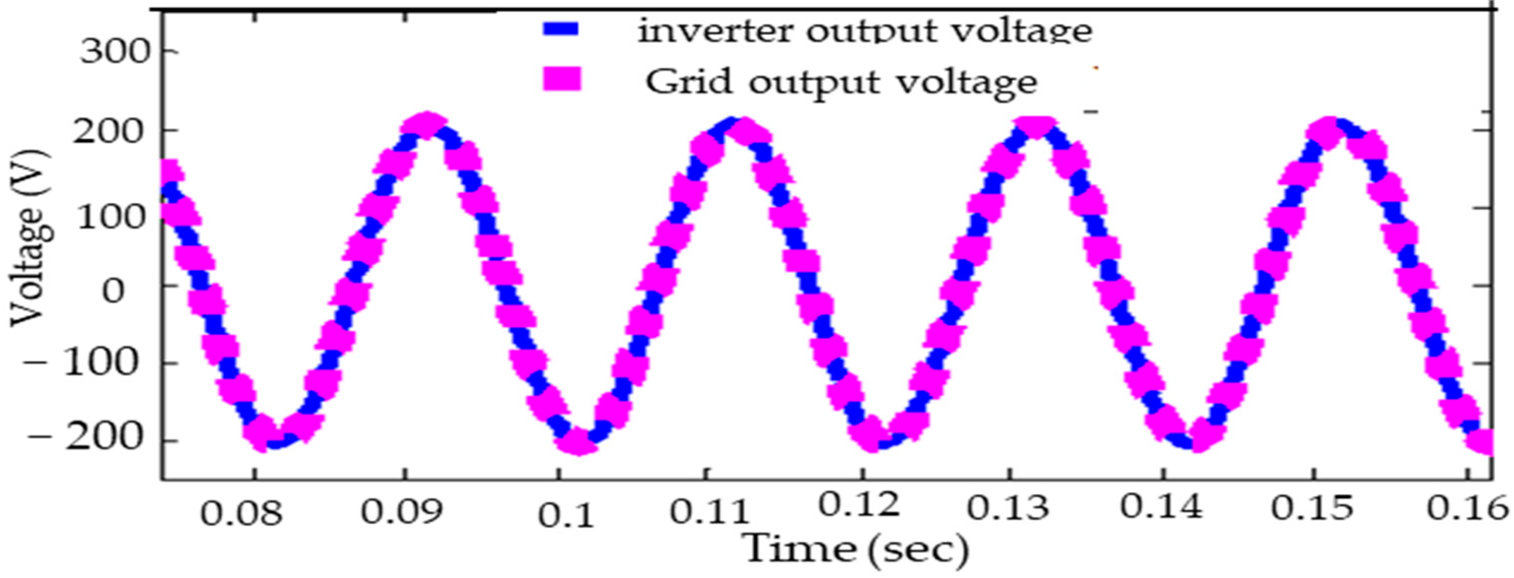
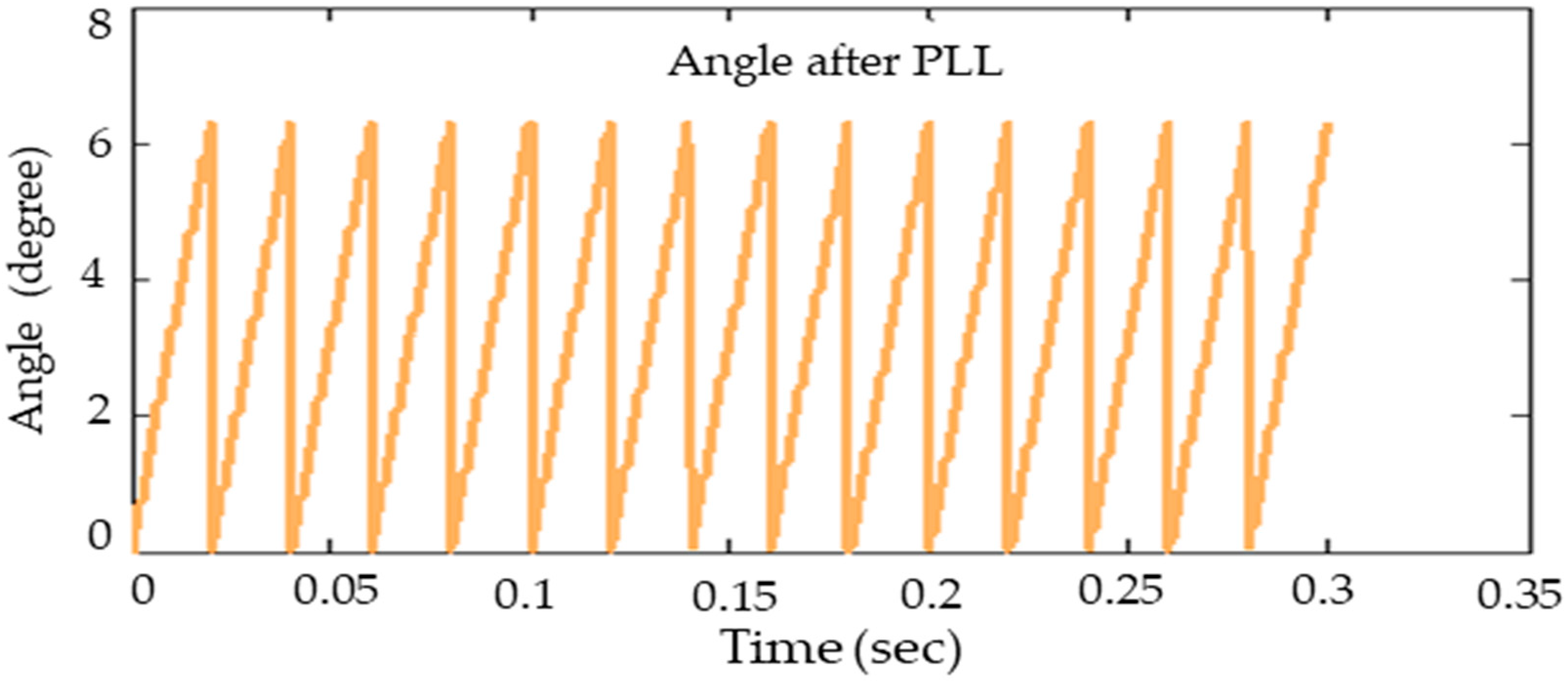
4.6. Test Simulation Results of Inverter Synchronization

The SVPWM modulation technique and the PLL block are employed to achieve the system’s primary objective. The gate signal control adopted an inverter in the studied PV system through the SVPWM-based feedback controller. As shown by the simulation results, when the input voltage of 220 V and the frequency of 50 Hz are applied to the grid, the voltage is passed to the PLL block, generating the output frequency, angle, and sinusoidal signals after processing. Figure 22 demonstrates the angle graph obtained from the PLL block.

The PLL block gives the output of the pure sine wave, which is the input for the SVPWM along with the inverter current. SVPWM is a type of pulse width modulation. It generates the signals that proceed into the inverter. This is how the voltages of the inverter and grid are synchronized through this implemented feedback system. Figure 23 and Figure 24 show the final results of synchronization. The grid provided 220 V. After synchronization, the results show that the inverter block gives the three-phase voltages, which are approximately 220 V and 120° apart.

Figure 25 presents the current for the inverter after synchronization. The value of the current is 45 A. As a result of grid synchronization, the PV system output provides reductions of up to 218 V and a maximized current value of up to 45 A, resultingly providing an output power of 9800 W.

5. Conclusions and Future Implications

This study investigated a generalized PV system with an MPPT controller algorithm constructed using the P&O technique; however, DC/DC converter, DC/AC inverter, and synchronized grid components were applied. The proposed system considers the variable resistive load to examine the consequence of load fluctuation on the PV system’s output power, voltage, and current under MATLAB/Simulink software. Firstly, this paper developed a generalized PV module that resembles the parameters specified in the mask for any PV module of interest. Secondly, the PV array BP MSX 120 array simulations revealed that the suggested system is meticulous because the current–voltage spectra are identical to the datasheet. The same PV array with a boost converter was examined with sudden changes in irradiance, temperature, and variable resistive load. The presented simulation results indicate that the PV output power, voltage, and current are affected by temperature and solar radiation deviations. However, the alteration in load fails to agitate the PV array’s result. Furthermore, the presented results demonstrate that the P&O-based MPPT controller accurately tracks the MPP of PVs during variable climate conditions. Finally, this study successfully synchronized the proposed model with the grid. The following are recommendations from this study to be adopted in the future:

• The methodology is simple and adaptive; therefore, it is economical for future use.
• The maximum power point can be tracked in varying environmental conditions; thus, it is quite appropriate to the areas where the environmental conditions vary abruptly.
• This technique is highly efficient compared to others; therefore, it is quite helpful for developing countries. Incorporating energy management strategies using advanced tools is essential when developing MPPT algorithms for photovoltaic systems.
• In the future, another recommended method is to use a variable step size using an advanced machine learning method and data analytics that adjusts the step size based on the difference between the PV output power and the reference power. This strategy increases the step size when the difference is significant and decreases it when the difference is slight, which can improve the convergence rate and reduce oscillations.
• Furthermore, advanced control techniques, such as model predictive control (MPC) and fuzzy logic control (FLC), have been suggested to enhance the performance of the P&O method. These methods use a mathematical model of the PV system and a feedback loop to adjust the operating point, which can improve the accuracy and stability of the control.
• In conclusion, while the P&O method is an effective and widely used algorithm for tracking the MPP of a PV system, it does have limitations that can affect its performance. These limitations can be addressed in future research by introducing modifications and advanced control techniques that can improve the accuracy, stability, and efficiency of the control.
• The technique is user-friendly as it is simple, thus it is quite appropriate for future use.
• Intelligent MPPT tracking models effectively analyze the system’s behavior under various conditions. This allows the identification of optimal settings for the MPPT algorithm and energy management strategies to maximize energy efficiency and minimize losses.
• Another essential tool is data analytics, which can provide insights into energy consumption patterns and enable predictive maintenance to reduce downtime and optimize performance. Additionally, integrating energy storage systems, such as batteries, can provide backup power and increase the system’s overall efficiency. By utilizing these advanced tools and strategies, developers can design MPPT algorithms that effectively manage energy and improve the performance and reliability of photovoltaic systems in the tech world.

References

1. Abdelsalam, A.K.; Massoud, A.M.; Ahmed, S.; Enjeti, P.N. High-performance adaptive Perturb and observe MPPT technique for photovoltaic-based microgrids. IEEE Trans. Power Electron. 2011, 26, 1010–1021. [Google Scholar] [CrossRef]
2. Katche, M.L.; Makokha, A.B.; Zachary, S.O.; Adaramola, M.S. A Comprehensive Review of Maximum Power Point Tracking (MPPT) Techniques Used in Solar PV Systems. Energies 2023, 16, 2206. [Google Scholar] [CrossRef]
3. Mohanty, P.; Bhuvaneswari, G.; Balasubramanian, R.; Dhaliwal, N.K. MATLAB based modeling to study the performance of different MPPT techniques used for solar PV system under various operating conditions. Renew. Sustain. Energy Rev. 2014, 38, 581–593. [Google Scholar] [CrossRef]
4. Abbas, S.Z.; Kousar, A.; Razzaq, S.; Saeed, A.; Alam, M.; Mahmood, A. Energy management in South Asia. Energy Strateg. Rev. 2018, 21, 25–34. [Google Scholar] [CrossRef]
5. Ounnas, D.; Ramdani, M.; Chenikher, S.; Bouktir, T. An Efficient Maximum Power Point Tracking Controller for Photovoltaic Systems Using Takagi–Sugeno Fuzzy Models. Arab. J. Sci. Eng. 2017, 42, 4971–4982. [Google Scholar] [CrossRef]
6. Eldin, S.A.S.; Abd-Elhady, M.S.; Kandil, H.A. Feasibility of solar tracking systems for PV panels in hot and cold regions. Renew. Energy 2016, 85, 228–233. [Google Scholar] [CrossRef]
7. Das, N.; Wongsodihardjo, H.; Islam, S. Modeling of multi-junction photovoltaic cell using MATLAB/Simulink to improve the conversion efficiency. Renew. Energy 2015, 74, 917–924. [Google Scholar] [CrossRef]
8. Manoharan, P.; Subramaniam, U.; Babu, T.S.; Padmanaban, S.; Holm-Nielsen, J.B.; Mitolo, M.; Ravichandran, S. Improved Perturb and Observation Maximum Power Point Tracking Technique for Solar Photovoltaic Power Generation Systems. IEEE Syst. J. 2021, 15, 3024–3035. [Google Scholar] [CrossRef]
9. Abbas, S.Z.; Ali, Z.; Mahmood, A.; Haider, S.Q.; Kousar, A.; Razzaq, S.; Hassan, T.U.; Su, C.L. Review of Smart Grid and Nascent Energy Policies: Pakistan as a Case Study. Energies 2022, 15, 7044. [Google Scholar] [CrossRef]
10. Keles, C.; Alagoz, B.B.; Akcin, M.; Kaygusuz, A.; Karabiber, A. A photovoltaic system model for Matlab/Simulink simulations. In Proceedings of the 4th International Conference on Power Engineering, Energy and Electrical Drives, Istanbul, Turkey, 13–17 May 2013; pp. 1643–1647. [Google Scholar] [CrossRef]
11. Esram, T.; Chapman, P.L. Comparison of photovoltaic array maximum power point tracking techniques. IEEE Trans. Energy Convers. 2007, 22, 439–449. [Google Scholar] [CrossRef]
12. Ali, Z. Fault Detection and Classification in Hybrid Shipboard Microgrids. In Proceedings of the 2022 IEEE PES 14th Asia-Pacific Power and Energy Engineering Conference (APPEEC), Melbourne, Australia, 20–23 November 2022; pp. 1–6. [Google Scholar]
13. Vaikundaselvan, B.; Sivaraju, S.S.; Sivan Raj, C.; Palraj, P. Design and analysis of MPPT based buck boost converter for solar photovoltaic system. Int. J. Electr. Eng. Technol. 2020, 11, 253–270. [Google Scholar]
14. Stember, L.H.; Huss, W.R.; Bridgman, M.S. A Methodology for Photovoltaic System Reliability & Economic Analysis. IEEE Trans. Reliab. 1982, R-31, 296–303. [Google Scholar] [CrossRef]
15. Vinod; Kumar, R.; Singh, S.K. Solar photovoltaic modeling and simulation: As a renewable energy solution. Energy Rep. 2018, 4, 701–712. [Google Scholar] [CrossRef]
16. Bouselham, L.; Hajji, M.; Hajji, B.; Bouali, H. A New MPPT-based ANN for Photovoltaic System under Partial Shading Conditions. Energy Procedia 2017, 111, 924–933. [Google Scholar] [CrossRef]
17. Ali, Z.; Terriche, Y.; Hoang, L.Q.N.; Abbas, S.Z.; Hassan, M.A.; Sadiq, M.; Su, C.-L.; Guerrero, J.M. Fault Management in DC Microgrids: A Review of Challenges, Countermeasures, and Future Research Trends. IEEE Access 2021, 9, 128032–128054. [Google Scholar] [CrossRef]
18. Javed, S.B.; Mahmood, A.; Abid, R.; Shehzad, K.; Mirza, M.S.; Sarfraz, R. Implementation of Generalized Photovoltaic System with Maximum Power Point Tracking. In Proceedings of the 2nd International Multi-Disciplinary Conference, Gujrat, Pakistan, 19–20 December 2016. [Google Scholar]
19. Naik, J.; Dhar, S.; Dash, P.K. Adaptive differential relay coordination for PV DC microgrid using a new kernel based time-frequency transform. Int. J. Electr. Power Energy Syst. 2019, 106, 56–67. [Google Scholar] [CrossRef]
20. Filho, N.d.M.; Cardoso Diniz, A.S.A.; Vasconcelos, C.K.B.; Kazmerski, L.L. Snail trails on PV modules in Brazil’s tropical climate: Detection, chemical Properties, bubble formation, and performance effects. Sustain. Energy Technol. Assess. 2022, 54, 31–35. [Google Scholar] [CrossRef]
21. Drif, M.; Bahri, M.; Saigaa, D. A novel equivalent circuit-based model for photovoltaic sources. Optik 2021, 242, 167046. [Google Scholar] [CrossRef]
22. Khamis, A.; Mohamed, A.; Shareef, H.; Ayob, A.; Aras, M.S.M. Modelling and simulation of a single phase grid connected using photovoltaic and battery based power generation. In Proceedings of the 2013 European Modelling Symposium, Manchester, UK, 20–22 November 2013; pp. 391–395. [Google Scholar] [CrossRef]
23. Hayder, W.; Ogliari, E.; Dolara, A.; Abid, A.; Ben Hamed, M.; Sbita, L. Improved PSO: A comparative study in MPPT algorithm for PV system control under partial shading conditions. Energies 2020, 13, 2035. [Google Scholar] [CrossRef]
24. Kenneth, A.P. Design of Dc-Dc Converter with Maximum Power Point Tracker Using Pulse Generating (555 Timers) Circuit for Photovoltaic Module. Int. J. Sci. Eng. Res. 2012, 3, 4. [Google Scholar]
25. Tobias, R.R.; Mital, M.E.; Lauguico, S.; Guillermo, M.; Naidas, J.R.; Lopena, M.; Dizon, M.E.; Dadios, E. Design and Construction of a Solar Energy Module for Optimizing Solar Energy Efficiency. In Proceedings of the 2020 IEEE 12th International Conference on Humanoid, Nanotechnology, Information Technology, Communication and Control, Environment, and Management (HNICEM), Manila, Philippines, 3–7 December 2020. [Google Scholar] [CrossRef]
26. Alturki, F.A.; Al-Shamma’a, A.A.; Farh, H.M.H. Simulations and dSPACE real-time implementation of photovoltaic global maximum power extraction under partial shading. Sustainability 2020, 12, 3652. [Google Scholar] [CrossRef]
27. Gradella Villalva, M.; Rafael Gazoli, J.; Ruppert Filho, E. Modeling And Circuit-based Simulation Of Photovoltaic Arrays. Eletrônica Potência 2009, 14, 35–45. [Google Scholar] [CrossRef]
28. Villalva, M.G.; Gazoli, J.R.; Ruppert Filho, E. Modeling and circuit-based simulation of photovoltaic arrays. In Proceedings of the 2009 Brazilian Power Electronics Conference, Bonito-Mato Grosso do Sul, Brazil, 27 September–1 October 2009; Volume 14, pp. 1244–1254. [Google Scholar] [CrossRef]
29. Ali, S.W.; Verma, A.K.; Terriche, Y.; Sadiq, M.; Su, C.L.; Lee, C.H.; Elsisi, M. Finite-Control-Set Model Predictive Control for Low-Voltage-Ride-Through Enhancement of PMSG Based Wind Energy Grid Connection Systems. Mathematics 2022, 10, 4266. [Google Scholar] [CrossRef]
30. Algarín, C.R.; Giraldo, J.T.; Álvarez, O.R. Fuzzy logic based MPPT controller for a PV system. Energies 2017, 10, 2036. [Google Scholar] [CrossRef]
31. Soltani, S.; Kouhanjani, M.J. Fuzzy logic type-2 controller design for MPPT in photovoltaic system. In Proceedings of the 2017 Conference on Electrical Power Distribution Networks Conference (EPDC), Semnan, Iran, 19–20 April 2017; pp. 149–155. [Google Scholar] [CrossRef]
32. Rafeeq Ahmed, K.; Sayeed, F.; Logavani, K.; Catherine, T.J.; Ralhan, S.; Singh, M.; Prabu, R.T.; Subramanian, B.B.; Kassa, A. Maximum Power Point Tracking of PV Grids Using Deep Learning. Int. J. Photoenergy 2022, 2022, 1123251. [Google Scholar] [CrossRef]
33. Takruri, M.; Farhat, M.; Barambones, O.; Ramos-Hernanz, J.A.; Turkieh, M.J.; Badawi, M.; AlZoubi, H.; Sakur, M.A. Maximum power point tracking of PV system based on machine learning. Energies 2020, 13, 692. [Google Scholar] [CrossRef]
Figure 1. Block Diagram of Solar PV System.
Energies 16 03638 g001
Figure 2. The single-diode circuit model of a PV device.
Energies 16 03638 g002
Figure 3. The schematic block diagram of PV module.
Energies 16 03638 g003
Figure 4. The circuit diagram of DC/DC converter.
Energies 16 03638 g004
Figure 5. The flowchart diagram of the studied P&O algorithm.
Energies 16 03638 g005
Figure 6. The Simulink model of the studied MPPT for a generalized PV system.
Energies 16 03638 g006
Figure 7. The three-phase inverter (a) and (b) parameters for PWM pulse generator.
Energies 16 03638 g007
Figure 8. Space Vector Corresponding to Each Switching State [23].
Energies 16 03638 g008
Figure 9. Internal structure of studied VPWM block.
Energies 16 03638 g009
Figure 10. The proposed PV system.
Energies 16 03638 g010
Figure 11. The feature graphs of studied PV array BP MSX 120 as a function of varying solar irradiation (G).
Energies 16 03638 g011
Figure 12. The feature curves of PV array BP MSX 120 as a function of temperature (T).
Energies 16 03638 g012
Figure 13. The PV output current, power, and voltage (V) under step variations in irradiation (G).
Energies 16 03638 g013
Figure 14. The output current (A), power (W), and voltage (V) of boost converter during sudden variations in irradiation (G).
Energies 16 03638 g014
Figure 15. The effect of temperature (T) variation on PV output current, power, and voltage (V).
Energies 16 03638 g015
Figure 16. Output power (W), current (A), and voltage (V) of boost converter for step change in temperature (T).
Energies 16 03638 g016
Figure 17. The test system result with load of 20 Ω: PV output power, voltage, and current (A).
Energies 16 03638 g017
Figure 18. The studied PV system output power, current, and voltage under 40 Ω loads.
Energies 16 03638 g018
Figure 19. Three-phase power inverter output current waveform.
Energies 16 03638 g019
Figure 20. The waveform of three-phase inverter phase to ground output voltage.
Energies 16 03638 g020
Figure 21. Three-phase inverter phase to phase output voltage signal.
Energies 16 03638 g021
Figure 22. The inverter and grid output voltage (angle from PLL block).
Energies 16 03638 g022
Figure 23. The synchronized voltages.
Energies 16 03638 g023
Figure 24. Three-phase voltages after synchronization with grid.
Energies 16 03638 g024
Figure 25. The output currents of three-phase inverter.
Energies 16 03638 g025