Multi-Period Portfolio Optimization with Investor Views under Regime Switching


Department of Mechanical and Industrial Engineering, University of Toronto, 5 King’s College Road, Toronto, ON M5S 3G8, Canada
*
Authors to whom correspondence should be addressed.
J. Risk Financial Manag. 2021, 14(1), 3; https://doi.org/10.3390/jrfm14010003
Submission received: 1 December 2020
/
Revised: 20 December 2020
/
Accepted: 21 December 2020
/
Published: 23 December 2020
(This article belongs to the Special Issue Financial Optimization and Risk Management)
Abstract
:We propose a novel multi-period trading model that allows portfolio managers to perform optimal portfolio allocation while incorporating their interpretable investment views. This model’s significant advantage is its intuitive and reactive design that incorporates the latest asset return regimes to quantitatively solve managers’ question: how certain should one be that a given investment view is occurring? First, we describe a framework for multi-period portfolio allocation formulated as a convex optimization problem that trades off expected return, risk and transaction costs. Using a framework borrowed from model predictive control introduced by Boyd et al., we employ optimization to plan a sequence of trades using forecasts of future quantities, only the first set being executed. Multi-period trading lends itself to dynamic readjustment of the portfolio when gaining new information. Second, we use the Black-Litterman model to combine investment views specified in a simple linear combination based format with the market portfolio. A data-driven method to adjust the confidence in the manager’s views by comparing them to dynamically updated regime-switching forecasts is proposed. Our contribution is to incorporate both multi-period trading and interpretable investment views into one framework and offer a novel method of using regime-switching to determine each view’s confidence. This method replaces portfolio managers’ need to provide estimated confidence levels for their views, substituting them with a dynamic quantitative approach. The framework is reactive, tractable and tested on 15 years of daily historical data. In a numerical example, this method’s benefits are found to deliver higher excess returns for the same degree of risk in both the case when an investment view proves to be correct, but, more notably, also the case when a view proves to be incorrect. To facilitate ease of use and future research, we also developed an open-source software library that replicates our results.
1. Introduction
Since Markowitz formulated portfolio selection as an optimization problem trading off risk and return over sixty years ago, mean-variance optimization has occupied a central role in constructing portfolios in both academic literature, and industry (Markowitz 1952). The reasons for its success are diverse. The model was the first to quantify the benefits of diversification towards reducing portfolio risk. Further, it simplified the portfolio selection problem by introducing the concept of an efficient frontier. On this delimitating line or frontier, we can find the portfolio with the highest return for a given level of risk. Despite its vast success, the model has its drawbacks. To arrive at a mean-variance portfolio, an optimization problem is solved for one fixed period: hours, days, months, and years. However, an investor’s end goal is broader than what could be achieved by a single mean-variance portfolio. The investor cares about maximizing their wealth over their entire investment period, which could last until a significant event or purchase, their lifetime or many generations (sovereign wealth funds). Superimposing one static set of returns and risk completely ignores the time-varying properties of asset prices over a long period of time. To address this drawback, we propose a reactive multi-period portfolio optimization framework that allows the direct incorporation of investor views and quantitatively generated degrees of confidence in each view on behalf of the investor.
Multi-period optimization (MPO) is a promising research area that allows us to optimize portfolio holdings for the immediately adjacent time period simultaneously and multiple periods beyond it. Considering only one period at a time, single-period mean-variance optimization is a sub-optimal nearsighted strategy. The objective for the current period, unlike the real world, is oblivious to unavoidable future constraints and, at a minimum, unaware of reasonable expectations for further future periods. Suppose our long-term return forecast encourages us to build a large position in one asset; however, our short term return forecast is negative. In this case, an optimal solution might be to buy over periods of negative returns to prepare for the long term expectation, a solution not easily incorporated in a single period setting.
Similarly, we can incorporate known macroeconomic events such as the US election directly into upcoming future periods. Suppose a reduction in portfolio holdings is desirable to prepare for the event. In that case, it can be expressed in MPO as a forecasted increase or a hard constraint of the underlying securities’ risk in a future period. Reducing the portfolio size over multiple periods would likely achieve this with lower market impact as opposed to one period. Using MPO, the investor also gains the ability to incorporate time-varying return predictions into one model, e.g., mean reversion or alpha decay (Boyd et al. 2017). This subset of examples serves to showcase the vast potential that MPO has to improve on the existing single period models.
Starting with Samuelson (1969) and Merton (1969)’s work, the literature on multi-period optimization (MPO) has focused on dynamic programming, which appropriately incorporates updated information for each period in the sequence of trades (Gârleanu and Pedersen 2013). Unfortunately, applying dynamic programming to the problem of trade selection is impractical for non-trivial cases due to the ‘curse of dimensionality’ (Powell 2007). Most studies focusing on dynamic programming only include simple objectives and constraints and a minimal number of assets. Various approximations to the dynamic programming problem are employed to achieve tractability, such as approximate dynamic programming or simpler formulations that generalize SPO into MPO (Boyd et al. 2014).
The method we will be leveraging in this article was recently introduced by Boyd et al. (2017) and consists of a relaxation from dynamic programming’s consideration of the entire time horizon. Successfully used in many industrial applications, model predictive control (MPC) incorporates new information into the optimization problem. At each time step, a multi-period optimization problem using information known at time T is solved for H periods ahead. Despite obtaining optimal actions for multiple time periods, only the first period’s actions are implemented, and the optimization problem is solved anew with updated information gained at time . We apply this receding horizon procedure to the MPO setting and simplify the full horizon dynamic programming problem while maintaining fast reaction times to changing financial markets. Applications to finance include portfolio optimization (see Herzog et al. 2007; Nystrup et al. 2019), optimal trade execution (Anis and Kwon 2020) and index tracking (Primbs and Sung 2008). Using the same MPO framework as (Boyd et al. 2017), Nystrup et al. (2019) leverage multi-period forecasts in order to minimize the chances of the portfolio falling below a certain level relative to its previous peak, i.e., achieve a lower maximum drawdown.
Boyd et al. (2017) demonstrate that this MPO method remains computationally tractable since it leverages convex programming throughout, can incorporate many costs and constraints and improves the risk-return frontier over SPO for daily equity trading in an ex-post example. From an optimality perspective, it is possible to produce a bound on the optimal performance for the dynamic trading of a portfolio of assets over a finite time horizon (Boyd et al. 2014). This performance bound can be used to judge the performance of any sub-optimal policy. While there is no theoretical guarantee of the performance of the method we are using, Boyd et al. show through Monte Carlo simulations that its results are typically close to the optimal performance bound. Although this optimization method is designed to look into the future, there is no set optimal horizon H to use. This article analyzes the results of portfolio allocation performance across one, two and five-period horizons.
We leverage the Black-Litterman (BL) model to generate more stable risk and return estimates for the optimization problem while avoiding common pitfalls found in direct and risk factor model-based estimation. Even in MPO, the mean-variance portfolio remains the core of portfolio optimization. However, when attempting to use the original Markowitz mean-variance optimization model for portfolio allocation decisions, the resulting portfolios are often uninvestable. Green and Hollifield (1992) documents the tendency of mean-variance portfolios to be skewed by having large positions in only a small subset of assets, thus going against the very concept behind their inception, diversification. Similarly, the model would almost always result in large short positions in many assets when allowing short positions. These troublesome results stem from two well-documented problems. First, portfolio managers tend to be extremely knowledgeable only on a specific set of assets, while a standard optimization model requires them to produce both return and risk estimates across all assets. We know that estimation errors can cause mean-variance optimized portfolios to perform poorly (see Michaud 1989; DeMiguel et al. 2009). Second, as a compounding effect, mean-variance portfolios are extremely sensitive to the return assumptions used. When any constraints are introduced to the optimization problem, a surprisingly small change to the return estimate of even one asset shifts half the portfolio’s allocation of assets while leaving the portfolio’s return and variance unchanged (Best and Grauer 1991).
Since estimation error is a leading cause of unexpected results from mean-variance optimization, significantly reducing the parameters to estimate also improves the mean-variance results. As mitigation, Fama and French (1992) introduced size and book-to-market equity factors that, when combined, capture the cross-sectional variation in stock returns. Leveraging explainable factors as drivers of returns enables financial practitioners to reduce the need to estimate parameters for a full risk covariance matrix to only , where n is the number of assets and m is the number of explanatory factors. Although extremely popular in academia and industry, implementing factor models in practice is not trivial. The presence of correlated factors can cause unit factor portfolios that are unintuitive to even experienced practitioners. Further, using trailing averages of factor returns implies a follower momentum strategy at the factor level without strong empirical justifications (Carvalho 2016).
Different mathematical techniques can also be employed in order to reframe the problem of portfolio selection. Credibility theory has been used to expand from traditional MVO to a fuzzy multiobjective model that also includes liquidity constraints beyond risk and return measures (Garcia et al. 2020). Similarly, uncertainty theory can be used to introduce new sources of background risk (income shortages, health-related expenses) that affect individual investors’ risk preferences into the portfolio selection problem (Huang and Yang 2020). Models using different choices of risk measures (semi-variance) and objectives (entropy, price-to-earnings ratio, satisfaction functions and environmental, social and governance (ESG) scores) have also been shown to be good alternatives to traditional MVO (see Chen and Xu 2019; Garcia et al. 2019; Mansour et al. 2019; Garcia et al. 2019).
As a widely-known approach to solving the Markowitz model’s problems, Black and Litterman (1992) developed their namesake model that combined the mean-variance optimization framework with Sharpe’s capital asset pricing model (CAPM) and applied it to global assets. The model starts with a baseline of global equilibrium returns defined as the asset returns that would stabilize the global supply-demand of risk assets. In practice, these returns are equivalent to portfolio holdings that are market capitalization-weighted, proportionally more allocated to better-capitalized countries (Sharpe 1964). Layered on top of the baseline equilibrium returns, the model allows an investor to incorporate their own return views for the areas where they have expertise while leaving the remaining assets to be allocated according to equilibrium returns. This approach addresses both inadequacies that exist in the standard mean-variance optimization. Managers are empowered to focus only on their subset of views while the layered approach anchors the final result to the well-diversified market capitalization-weighted portfolio. The enrichment of baseline returns with dynamic investor views is the reasoning behind using the BL model at our framework’s core.
Although conceptually simple, the Black Litterman (BL) model is imperfect. BL is static and effectively single-period. Once the target weights are obtained, portfolio managers are expected to actively track the results of their view and reoptimize upon any changes in their view or confidence levels. Using data-driven methods to infer dynamic confidence levels in an investment view eliminates the need to choose an entry/exit point and enables its expansion to multiple periods without further investor input. Further, BL is relatively complex to understand even for a quantitative researcher, as evidenced by the number of papers dedicated to presenting it in more straightforward ways (see He and Litterman 2002; Idzorek 2004; Walters 2007). We introduce a regime-switching component that makes the model reactive to market regime changes and, in turn, reduces the work needed to interact with the model.
A growing set of literature shows that we can exploit shorter-term trends in both returns and volatility, similar to what we propose in this article. Hidden Markov models (HMM) have been successfully used in speech recognition (Jelinek 1997), natural language modelling (Manning and Schutze 1999) and the analysis of biological sequences such as proteins and DNA (Krogh et al. 1994). Ang and Timmermann (2012) explored their predictive power on financial variables and discovered that they could be used across various financial markets and macro variables. HMMs can describe the financial market’s tendency to abruptly change its behaviour and the propensity for financial variables to maintain their behaviour over more extended periods. Within the field of finance, their application is referred to as regime-switching. Incorporating their predictions within mean-variance optimization has been found to improve portfolio performance in multiple ways. Nystrup et al. (2017) found that regime based asset allocation improves portfolio return and risk metrics over rebalancing using static weights. Costa and Kwon (2019) used regime-switching to build factor models to assist with the difficult problem of estimating covariances and demonstrated higher ex-post return for the same level of risk compared to a nominal factor model.
Despite numerous examples of using regime-switching in finance, there is a dearth of literature on the benefits of tactically improving the BL returns and risk through regime-switching predictions. The only directly connected article uses a two-state regime-switching model as the return estimates provided to the Black-Litterman model. It finds that regime-switching returns outperform directly estimated returns (Fischer and Seidl 2013). Our approach is different; the BL equilibrium returns are kept intact as a base while our goal is to improve the investor views. This article extracts predicted returns from the most straightforward HMM consisting of only two states and uses them to compute dynamic confidence values in investment views. The reason for choosing a two-state model as opposed to more is two-fold. First, Nystrup et al. (2019) find no benefit from increasing the number of states above two out of sample when using long-term daily data. Second, a simpler model is less likely to overfit the training data and is more likely to be embraced in practice due to its increased interpretability. The lack of interpretability is a significant barrier to model adoption by investors. By leveraging regime-switching, we propose that it is possible to compute a practical dynamic confidence level by comparing the investor view to the regime-switching predicted view return. This dynamic comparison serves to remove the BL model’s dependency from correctly chosen confidence levels or entry and exit points.
Our essential assumptions regarding the trading frequency should be noted, given our use of both market equilibrium returns and regime-switching models based on daily return data. Market equilibrium returns are based on supply and demand reaching a stable balance. At higher frequencies (tick, second, minute), we expect this stable balance to be more fleeting, making market microstructure and short term effects much more critical. Conversely, it is more likely to observe stable supply-demand equilibria to base trading decisions on at a lower frequency. Further, our regime-switching training was performed over multiple years, with only two states (bull and bear), making the predictive power at a higher frequency (intraday or daily) lower. That said, reacting to a regime change faster is better than reacting to a regime change slower. Therefore, the interval we chose to strike a balance between these two factors was a weekly trading frequency and was applied in most simulations performed.
Introducing a more dynamic allocation as proposed (based on direct market data) can lead to potential problems that we mitigate against, namely, return instability and overtrading. Since regime-switching models using higher frequency data are faster to update their confidence in each regime, this can lead to fleeting regimes and unnecessarily high portfolio reallocation. To prevent this, similar to Nystrup et al. (2015), we incorporate a minimum probability threshold to overcome before allowing the regime to change. The threshold reduces regime jitter at the expense of a slightly slower reaction to regime changes. We know that transaction costs can be high when trades are made frequently (Kolm et al. 2014) and that SPO can be augmented to efficiently include many types of costs and constraints in the portfolio selection (Lobo et al. 2007). Therefore, we incorporate transaction costs into the portfolio optimization. These two changes, regime-switching thresholds and transaction cost optimization, serve to mitigate the potential adverse effects we mentioned above. Market microstructure issues such as liquidating large positions or information leakage to other participants are only partially addressed by using a temporary impact cost component. The first to introduce the concept of optimal intraday execution of portfolio transactions, Almgren and Chriss (2001) developed a simple linear temporary impact cost model and introduced efficient frontiers trading off the minimum expected cost versus a given level of uncertainty. However, since its introduction, the field of optimal execution has advanced significantly through the introduction of permanent impact costs, dynamically adaptive strategies and stochastic volatility, among others (see Lorenz and Almgren 2011; Almgren 2012). Given our lower frequency of trading (daily or longer) and liquid developed country based ETFs, we do not focus further on this topic but note that it would be an exciting area of future research.
Overall, the proposed model improves traditional single-period mean-variance portfolios by incorporating multi-period trading and interpretable investment views into one easy-to-use framework. We leverage a multi-period portfolio optimization model introduced by Boyd et al. (2017) that approximates the entire trading range optimization by repeatedly optimizing smaller, more tractable consecutive sub-ranges. Although trading decisions are made for multiple periods in advance, only the next period trading decisions are executed. The model requires accurate risk and return estimates for the portfolio optimization, which we obtain from the BL model as the combination of the market portfolio and investment views. To mitigate against BL’s static nature and provide dynamism to the estimates, we propose a novel method of using regime-switching to determine each investment view’s confidence. We do not address the actual generation of investment views; instead, we focus on trading them effectively once provided.
1.1. Outline
The article is structured as follows: Section 2 introduces the multi-period optimization model based on receding horizon MPC. Section 3 presents the computation of risk and returns estimates needed to instantiate the portfolio optimization model. It starts by showing how the Black Litterman model is used to incorporate investor views in Section 3.1, then introduces the dynamic investor view confidence levels obtained through regime-switching in Section 3.3. It concludes with pseudo-code that details all the parts needed for the complete algorithm and simulation. Section 4 showcases our empirical results using this framework. Finally, Section 5 concludes.
1.2. Contribution
The main contributions to the existing literature are two-fold. First, we are the first to develop a multi-period optimization model to solve a portfolio allocation problem based on return and risk estimates from the Black Litterman (BL) model. As opposed to traditional dynamic programming, this method enables the optimization to be dynamic across time and, as such, allows new information to be incorporated as soon as it’s realized. This multi-period relaxation method aptly named receding horizon, is borrowed from model predictive control and was first introduced by Boyd et al. (2017). Given the increase in trading frequency over static models, convex transaction costs are also considered in the optimization objective. Second, we introduce a novel data-driven method to infer dynamically updated confidence levels for investment views. The confidence is obtained by computing the view’s regime expected return (based on each underlying asset’s current regime) and comparing it to the investor inputted expected return. The more the two forecasts are in agreement, the higher the confidence obtained and vice versa. Overall, the result is a framework that is reactive, numerically tractable and easy to use by a portfolio manager looking to trade researched investment views optimally. We have also developed an open-source software library that implements all of the methods in the paper and can be used to replicate our results easily: https://github.com/roprisor/alphamodel.
2. Multi-Period Optimization
Multi-period optimization (MPO) has shown great promise as a flexible solution for constructing optimal portfolios over multiple separate but connected time periods. The traditional mean-variance is designed for only one time period and, therefore, more fit for stationary risk and return assumptions. In practice, financial asset prices exhibit non-stationary behaviour, which is better incorporated in a multi-period optimization model. Academic literature has focused on dynamic programming, a method that has proven impractical for non-trivial cases due to the ‘curse of dimensionality’ (Powell 2007). Recently, Boyd et al. (2017) developed a model that generalizes from single-period optimization (SPO) to MPO. Its advantages include tractability and flexibility while still achieving near-optimal results. Through convex optimization for all objectives and constraints, the model can remain tractable despite introducing multiple periods and many constraints for each period. While there is no theoretical guarantee of the performance of the method we are using, Boyd et al. (2014) show through Monte Carlo simulations that its results are typically close to the optimal performance bound. This model, presented below, will be leveraged as a base for the framework presented in this paper.
At each time period T, a multi-period optimization problem using information (risk, return, and transaction cost estimates) known at time T is solved for H periods ahead, where . Despite obtaining optimal actions for multiple future time periods, only the first period’s actions are implemented, and the optimization problem is solved anew with updated information gained at time (see Figure 1a,b). This receding horizon procedure simplifies the full horizon dynamic programming problem while maintaining fast reaction times to changing financial markets.
A natural question that arises when considering the horizon for each multi-period optimization problem is how exactly we decide how many periods ahead the optimization should consider, i.e., what should H be? Let us consider the limiting values for H. As a minimum value, when , we are performing sequential single-period optimization. As a theoretical maximum, when , we are effectively considering the entire trading range all at once. Although possible, optimization across the entire trading range is impractical unless we have accurate return and risk forecasts that far into the future. Therefore, a practical value for H will depend heavily on the forecast horizon of our return and risk estimates. We will compare multiple values for H to validate its impact in the empirical results section.
2.1. Multi-Period Optimization Model
Consider a portfolio of n assets, plus a cash account, over a finite time horizon split into discrete time periods labeled . The time period in the model can be of arbitrary length however we will consider each period to be a trading day throughout this paper. Let denote the portfolio (or vector of holdings) at the beginning of time period t, where is the dollar value of asset i. implies a short position in asset i. As a corollary, when for , we call the portfolio long-only. Since asset represents the cash account, implies that at time t the portfolio is fully invested, i.e., we hold zero cash, all holdings are invested in non-cash assets. The total value of the portfolio, in dollars, at time t is expressed by .
Another way to describe the portfolio is through fractions of the entire dollar value or weights. Given a portfolio with holdings , the weights (or weight vector) are defined as . The portfolio weights always sum to one, by definition, , and are unitless (dollar holdings divided by portfolio total dollar value). Equivalent to the holdings scenario, the last weight is the fraction of the total portfolio value being held in cash.
Let be the dollar value of our trades in period t. We will assume that all trading happens at the beginning of each time period. implies that we bought dollars of asset i and implies the opposite, for . Normalizing the dollar value trades relative to the total portfolio value we obtain the normalized trades .
SPO only considers the most recent trade decision while ignoring any future periods in the current optimization. Effectively, SPO is the specific case of MPO where the forward horizon only includes one period. In MPO, we obtain the current trade vector by solving an optimization problem over a planning horizon that extends H periods into the future as illustrated in Figure 1a for times:
We develop the multi-period optimization problem from the core mean-variance objective: maximizing returns while minimizing risk and transaction costs. Let
denote our sequence of planned trades over the horizon. Given estimated returns , risk and transaction cost , a natural multi-period objective is to maximize the sum of risk-adjusted return over the horizon:
where and are variables, and are positive parameters used to scale the respective costs and the denotes an estimate rather than a known or realized quantity. These parameters are sometimes called hyper-parameters, analogous to the identically named parameters we obtain when fitting statistical models to data. The hyper-parameters can significantly affect the performance of the MPO method and should be chosen carefully through backtesting.
As noted earlier, although only the trades for period t are executed for each optimization looking H periods into the future, the model has both the ability to incorporate newly discovered information and to consider the optimal allocation of trading across all the H periods into the future. When , we are solving an SPO problem.
2.2. Degrees of Freedom
The optimization model purposefully leaves open multiple degrees of freedom required for it to be instantiated (Boyd et al. 2017). The performance analysis associated with the originally proposed model is done ex-post (using realized future data that could not be known when optimizing) with no future projections provided. To build a complete trading model, we fill in the missing components as follows:
- return and risk estimates: returns and risk are replaced by and generated from the Black Litterman model
- transaction cost estimates: remains the 3/2 transaction cost model
Since returns are represented as a vector , replacing the vector with Black Litterman estimates is straighforward.
2.2.1. Risk
Assuming the returns are randomly distributed, with covariance matrix , the variance of the portfolio return is given by
We obtain the traditional quadratic risk measure from the Black Litterman model covariance for period t,
We note that is an estimate of the return covariance based on sample data and model assumptions. The exact distribution of the process generating real asset price returns can never be known.
2.2.2. Transaction Cost
Trading in financial markets generally incurs a transaction cost, denoted as , where is the (dollar) transaction cost function. The model assumes that the transaction cost function is separable, i.e., the transaction cost breaks down into a sum of transaction costs for each individual asset. This assumption ignores the cointegration effect of asset prices at the high-frequency level which is a reasonable assumption given the period considered in our paper is one day. , a function from into , is the transaction cost function for asset i, period t.
Similar to Boyd et al. (2017), the model chosen for the transaction cost function is
where a, b, , V, and c are numbers and x is a dollar trade amount (Grinold and Kahn 2000). a represents the asset’s half-spread (half the bid-ask spread) at the beginning of the time period when trading occurs. This term is represented relative to the asset price and is therefore unitless. If desired, a can be increased by an amount representing broker fees expressed as a function of the dollar value traded. The second term represents the temporary impact cost of our trading. b is a positive constant of unit . V represents the total dollar value of the asset traded in the market in the current time period. The number reflects the asset price’s standard deviation over the most recent periods, expressed in dollar units. As mentioned by Boyd et al. (2017), a common rule of thumb is that trading one day’s volume is expected to move the price roughly by one day’s volatility. This would lead to a value of b around one. Given that c is linear in dollars traded x, we can use the third term to express differences between buying and selling an asset. If the term is ignored (), the cost is the same regardless of the trade direction. However, when , selling is more expensive than buying, which could reflect a market with difficulty borrowing stock to short sell or otherwise increased selling pressure (more sellers than buyers).
3. Return and Risk Estimates with Investor Views
Successful multi-period portfolio optimization relies on having a set of accurate risk and return estimates to produce trading decisions that perform well out of sample (see Green and Hollifield 1992; Michaud 1989; DeMiguel et al. 2009). In this paper, we leverage the Black Litterman (BL) model for risk and return estimates. BL aims to reduce estimation error by combining the market portfolio with a set of investor views. The market portfolio is a portfolio based on a condition that must be satisfied (all assets change hands; each seller finds a buyer). The investor views are expressed as portfolios that the investor provides a target return and confidence level for.
One of the most considerable drawbacks of the BL model is its static nature. It perfectly fits the category of single-period models that are not designed to adapt to changing market conditions optimally. Incorporating static by nature BL model risk and returns into multi-period optimization where they will be used repeatedly, as proposed in Section 2, requires at least one component to be dynamic. Since the market portfolio is fixed (only changes with market capitalization) and equilibrium returns mostly reflect parameter changes, the key to making the risk and returns estimates dynamic is the investment views. Our proposal replaces the static confidence levels in each investor view with dynamic values generated by a regime-switching model.
Regime switching has shown great value when applied to the financial markets (see Ang and Timmermann 2012; Fischer and Seidl 2013; Nystrup et al. 2017; Costa and Kwon 2019). The model’s underlying idea leverages the observation that asset prices exhibit time-varying behaviour, such as their tendency to exhibit trends in their statistical properties (means, standard deviations). Multiple return distributions called states fit to financial data are used as both explanatory variables of their past properties and predictors of their future properties. This model fits perfectly with the concept of investment views, which, once researched, are investors’ expectations of financial trends that will persist for some time in the future.
To sum up, multi-period portfolio optimization requires a set of risk and return estimates that we obtain from the Black Litterman model. This model incorporates investment views that are expected by the investor to exhibit trends. As such, in order to capture the confidence level (likelihood) that the expected trend is already underway or has ended, we use a regime-switching model. This combination allows us to construct our set of risk/return estimates, a needed building block for dynamic multi-period portfolio optimization, that quantitatively follow the trend of the expected investor views.
3.1. Black Litterman Model
The original Markowitz optimization model has at least two significant drawbacks. First, it tends to skew towards building large position weights in only a small subset of assets, effectively negating its original goal of diversifying across multiple assets (Green and Hollifield 1992). Second, it is notoriously sensitive to minute changes in the return assumptions used. A small change to the return estimate of only one asset can shift half of the portfolio allocation (Best and Grauer 1991). To counteract these well-documented problems, Black and Litterman (1992) developed a new model that combines the Markowitz mean-variance optimization with Sharpe’s CAPM through a Bayesian approach. Their model starts with a completely neutral view of the asset means (prior). The only reasonable definition of which—they argue—is the set of expected returns that would ensure the market is cleared if all investors had identical views (cleared implying that all assets are traded, each buyer finds a seller). Given this equilibrium state, their model allows investors to specify linear combinations of investment views that are overlayed on top (posterior). This overlay causes a subtle allocation shift from equilibrium depending on the strength of the investor’s conviction. Since each view’s confidence can be specified together with the overall willingness to diverge from equilibrium, the Black-Litterman model can counteract both problems with Markowitz optimization. The resulting weights are well diversified, and small changes in investor views of the asset means only exhibit localized effects, leaving most of the portfolio intact.
From a mathematical modelling perspective, let us assume there are n investable assets in our universe. Their returns r are driven by normal distributions with mean and a covariance matrix : . At equilibrium, all investors as a whole will hold the market portfolio . Therefore the equilibrium risk premiums are set such that, if all investors hold the same view, the demand for the assets equals the available supply (Black 1989). Assuming an average world risk tolerance which is represented by the risk aversion parameter , the equilibrium risk premiums are given by:
From a Bayesian perspective, the prior consists of the expected returns being normally distributed and centered at the equilibrium values (mean of ):
where is also a normally distributed random vector with zero mean and covariance matrix , being a scalar which represents the uncertainty of the CAPM prior.
To overlay investment theses on top of the CAPM prior, the investor also needs to define a set of views. The views are expressed such that the expected return of a portfolio p has a normal distribution with mean equal to q and a standard deviation given by . If we let K be the number of total views, P a matrix whose rows are the view portfolio weights and Q a K-vector of the expected returns of these portfolios.
Given the above, we can express the investor views as:
where is an unobservable normally distributed random vector with zero mean and a diagonal covariance matrix .
We now have all the pieces required to combine the CAPM equilibrium returns together with the investor views in a Bayesian framework. The result is a set of posterior expected returns that are distributed as , where the mean is given by:
and the covariance by:
For a detailed derivation of Equations (4) and (5), the reader is encouraged to refer to Meucci (2008)’s working paper that provides a detailed analysis of the original formulation and its re-casting into the more computationally stable posterior representations listed above.
Raised by Idzorek (2004), a problem with the original Black-Litterman model was that its formulation was meant to allow the incorporation of investor views, yet the process for doing so was complicated by the need to define uncertainty covariance values for each. This requirement was an unnecessary barrier preventing non-quantitative investors from adopting the framework more widely. To resolve this, Idzorek proposed specifying the investor’s confidence in the views expressed as a percentage, 0–100%, where the confidence measures the change in weight of the posterior from the prior estimate (0% confidence) to the conditional estimate (100% confidence). According to this methodology, a coefficient of uncertainty in the interval [0, ∞) is used to construct the uncertainty covariance from the view portfolio covariance as such:
Walters (2007) obtains a closed-form solution for Idzorek’s confidence interval formulation, which greatly simplifies the process of obtaining . This combined method allows investors without a quantitative model driving their investment theses to adapt their views to the Black-Litterman framework easily. Thus, the requirement is shifted from providing exact uncertainty covariance values to only providing a confidence value in the interval (0, 1]. In turn, Equations (6) and (7) transform these confidence values into model-driven uncertainty values.
3.2. Regime Switching Model
Our goal is to generate risk and return estimates that can be used to optimize repeatedly as time advances each period across the entire trading horizon. However, the Black Litterman (BL) model itself is static and, as such, does not lend itself to the dynamic incorporation of new information. To mitigate this problem, we leverage a regime-switching model that is well suited to predicting asset return trends and use it to generate dynamic confidence levels in each investor view. Once provided to the BL model, a view is considered both established and static until removed or manually edited by the investor. Considering the non-stationary nature of financial markets, the exact time a view is discovered might not be the best entry point. The investment thesis might either be too early or too late, which the model will not protect against. Further, any single view is not guaranteed to achieve consistent results over time, resulting in potential over-allocation to poorly performing views and hence under-allocation to strongly performing views over their lifetimes.
Financial market trends can change abruptly. Consequently, their return means, volatilities, and correlations also shift according to economic, political or behavioural trends that underlie asset valuation. Once established, changes tend to persist over extended periods, thus leading to observations such as the clustering of volatility first noted by Mandelbrot (1963).
Looking at the time series of returns for SPY, the most popular ETF tracking the S&P 500 Index (Figure 2a1), we can visually observe these shifts. Following periods of more subdued volatility, abrupt spikes materialize and cluster together. The U.S. market underwent a very long stretch of a calm bull market from 2009 to 2020. However, this period sharply contrasts to the global financial crisis in 2008 and the onset of the severe COVID-19 pandemic in 2020. Looking closer at the return densities for 2018–2020 (Figure 2b2), the difference between their shapes is apparent. None of the three years seem to be close to what Markowitz’s original theory assumes, a Bell curve. 2018 and 2019 have pronounced left tails, while 2020 is an outlier with wide left and right tails. Similar regime shifts, some periodic (expansions followed by recessions) and some unique (global events such as the recent COVID-19 pandemic), are found across a wide array of financial markets and macro variables (Ang and Timmermann 2012).
Regime switching attempts to exploit these clustering effects of financial time series to generate alpha and improve portfolio risk-reward metrics. Regime based asset allocation has been shown to improve portfolio metrics over rebalancing using static weights (Nystrup et al. 2015). In machine learning, the area focused on inferring a set of labels out of data (e.g., hidden regimes) is referred to as unsupervised learning. Due to the sequential nature of financial data, a natural choice to model regime transitions is a first-order Markov chain.
3.2.1. Markov Chains
A first-order Markov chain is a stochastic process describing a sequence of possible states in which the probability of the next state depends entirely on the previous state . More formally:
This memorylessness property allows us to loosen the i.i.d. assumption of more traditional non-sequential models. The model remains computationally tractable while incorporating past information into future probabilities of sequential data (Bishop 2006).
3.2.2. Hidden Markov Models
Hidden Markov models have been applied to speech recognition (Jelinek 1997), natural language modelling (Manning and Schutze 1999) and the analysis of biological sequences such as proteins and DNA (Krogh et al. 1994). The reason Markov chains are useful to model the shifting conditions of financial markets is that for each underlying state, we can attach a different probability distribution for the returns. For example, for a two-state chain, we can consider one state to represent an upwards trending (bull) market and the other state a downwards trending (bear) market. Similarly, for a three-state chain, the third state could represent a sideways (calm) market. We would expect each state’s probability distribution to reflect the financial market-relevant at the time. A bull market would be represented by a Gaussian distribution with positive mean and low variance, while a bear market would have a negative mean and high variance:
where and .
Such a combination of multiple unobservable (latent) states connected through a Markov chain is called a hidden Markov model. To build a hidden Markov model from our notation for a Markov chain, assuming we have observations , we introduce corresponding latent variables for each observation. We further assume that the latent variables are the ones forming a Markov chain such that and are independent given (memorylessness property, Equation (8)). The latent variables which we just introduced are designated to represent which state the observation pertains to. Each state has its emission probability distribution, the most basic case being a Gaussian distribution. Mathematically they are represented as discrete multinomial variables in a 1-of-K coding scheme. Because the underlying states depend on each other through a Markov chain and each variable is K dimensional, the transition probabilities between states correspond to a table of numbers we denote as A, the transition matrix. They are given by . In our case, since we utilized a two-state model, the conditional distribution of the current latent variable is given by:
Since the initial latent variable does not have a previous latent variable to form conditional distribution respective to, it has a marginal distribution represented by a vector of probabilities . Each element of the vector denoting the initial probability that the underlying state for the first observation was state k.
Specifying the probabilistic model is completed by defining the conditional distributions of the observed variables on the latent variables and , the set of parameters governing the distribution, . Thus, the joint probability distribution over both observed and latent variables is given by:
where is the set of all observations , same for , and denotes the set of parameters governing the model.
3.2.3. Estimation
The parameters of hidden Markov models are typically estimated by attempting to maximize the joint probability distribution in Equation (9) with respect to , also known as the maximum-likelihood method. The most popular methods to maximize the joint probability distribution are direct numerical maximization and the Baum-Welch algorithm, a special case of the expectation maximization (EM) algorithm (see Baum et al. 1970; Dempster et al. 1977). In this article, we utilized the Baum-Welch algorithm to extract the model parameters and latent variable probabilities.
The EM algorithm starts with an initial estimate of the model’s parameters, and A, which we can denote as . The core proposition decouples the numerical maximization into two steps: expectation (E step) and maximization (M step). In the E step, we use the old parameter values find the expected probability of the latent variables given the observations and (the posterior distribution of the latent variables). We can then use this to evaluate the expectation of the logarithm of the likelihood as a function of .
In the M step we maximize with respect to the parameters while holding constant the posterior distribution of the latent variables that we computed in the E step. The Baum-Welch algorithm has several variants, of which one of the more popular is the alpha-beta algorithm. Bishop (2006) has an excellent exposition of both the algorithms employed, EM and alpha-beta, which we will not reproduce here.
3.3. Dynamic View Confidence through Regime Switching
We can now focus our attention on using the newly obtained asset return regime-switching forecasts. As discussed at the beginning of Section 3 and Section 3.2, one of the drawbacks of the BL model remains the static inputs of view confidence. Since our multi-period optimization method requires frequent re-solving, the risk and return estimates need to be updated according to the newly available information. Therefore, we propose converting our regime-switching based forecasts into dynamic confidence levels for investor views.
The impact of an incorrect confidence forecast can be a significant drag on performance in the very competitive world of asset management. For example, in Figure 3, we track two opposite views considered ex-post: (long EWG, short SPY) versus (short EWG, long SPY). The delta between these two views peaks at over 125% at the end of 2007. This implies that there would have been a 1.25% performance gap between views for every 1% of portfolio allocation. To make matters more interesting, the winning view is counter to the generally accepted market equilibrium returns. Germany outperformed the United States by a surprising 50% over the 2005–2008 period. As always, when dealing with predictions, the problem is that not all investors would be able to correctly choose the right view all the time, never mind the right degree of confidence, without some kind of systematic process.
Regime switching can be used to completely remove the need to define a subjective degree of confidence in the investor views provided to the BL model. From Equation (3), we know that the expected return for an the investor’s view portfolio is expressed as . However, given that we have already estimated the underlying regimes driving each asset’s return, we can also compute it directly from these estimates:
where represents that the quantity was obtained from the most likely underlying regimes for the current sample of returns.
Since the investor has already specified their expectation for the view return to have mean , there are multiple methods we can employ to compute the confidence that should be assigned to it systematically. As a first method, we could focus on what quantity we are interested in for relative to the prediction. Specifically, a possible perspective on confidence could be to consider it to be the likelihood that the view return will be or better (Figure 4a):
Similarly, in a more simplistic fashion, we also consider the confidence in a given view to be akin to a neural network node that is activated when our estimated is greater than the investor’s input (Figure 4b). One of the most popular activation functions is the sigmoid function, largely owing to its step-like behaviour and ease of differentiation at all points (Bishop 2006). To adapt it to our current purpose, we need to incorporate two adjustments to the base sigmoid function. First, we add a slope parameter , which we could consider similar to the BL model confidence in the investor views. The steeper the activation slope, the faster the change in confidence level. As a result, a view that becomes in play will be reflected in estimated returns faster. Secondly, a scaling parameter is introduced defined as , where is the order of magnitude of x. Its purpose is to counteract the unwanted effects resulting from comparing tiny magnitude returns and expand the range of confidence values. The slope parameter value could be set through backtesting to match the shifts in realized view closely returns with the shifts in view confidence; however, great care needs to be placed on avoiding over-fitting. For this paper’s purposes, we used a higher base value of 4 for the slope parameter () to both avoid using views that might not be active and switch fast to active views once identified. The value of was computed for the scaling parameter since daily returns are on the order of magnitude of basis points. No further fitting was performed that could introduce bias in the results.
3.4. Multi-Period Portfolio Optimization with Investor Views
To instantiate the multi-period optimization model we described in Equation (1), we outlined the need for accurate and reactive risk and return estimates. Our proposal depends on three key components to achieving this. First, regime-switching forecasts for the underlying asset returns; second, a method to construct confidence levels for investment views from the forecasts; and third, risk and return estimates obtained from the Black Litterman (BL) model that integrates the investment views with the newly constructed confidence levels.
The Algorithm 1 pseudo-code illustrates in detail the entire simulation we propose in order to perform multi-period portfolio optimization while incorporating dynamic risk and return estimates from the BL model. For live trading, given a specific set of optimization hyper-parameters chosen carefully through backtesting, only the iteration of the loop for the most recent period T should be performed and, as such, only the trades applied. A natural question that arises while considering the structure of the algorithm is: what is the value of optimizing multiple periods ahead when is constant? We expect that the answer lies in the interplay between shifting weights to follow the return forecasts trend and the regime-switching component’s dynamicity. More specifically, when considering only one period at a time, each optimization will effectively try to adjust the portfolio weights as much as possible in the current period. This could be an optimal strategy if we know that there is no new information to incorporate shortly after. However, this is exactly what we are trying to achieve through the regime-switching and dynamic confidence component. Every time we reoptimize, we incorporate all the newly available asset return information and refit the regime-switching model, which, in turn, generates a more up to date set of returns to use. Increasing the number of trading periods beyond one gives the portfolio optimization the chance to trade off fast portfolio shifts against transaction costs that can be spread out across time. Every time some part of trading is best left for a period further than the current one, we would have new information to use that would be incorporated in new return and risk forecasts. The performance loss or benefit from incorporating multiple trading periods is addressed empirically in Section 4.3.
| Algorithm 1. Multi-Period Portfolio Optimization Simulation Pseudo-Code. |
 |
4. Empirical Results
The proposed multi-period portfolio optimization framework can be applied across a wide range of asset universes with an infinite number of combinations of investor views overlayed on the market portfolio. From a practical perspective, to show the promise of the framework, we focus on a numerical example comprising two opposing views. Especially in finance, forecasting is a challenging endeavour, as shown by the increasing number of assets shifting to passive investment vehicles (index tracking). It is impossible to know with certainty ahead of time if an investor’s view will realize. Therefore, a tricky trading scenario to test our framework is to provide it with both a ‘correct’ and an ‘incorrect’ view and observe how it updates its confidence in each view with each new price of information it is provided. While an investor would equally participate in both the upside of the ‘correct’ view and the downside of the ‘incorrect’ view, a successful quantitative model should be able to discover when the ‘incorrect’ view underperforms and, as such, reduce the downside exposure while leaving the upside in the ‘correct’ view case.
In this section, we first present our computational setup used for the simulations. Second, we present the regime-switching and dynamic confidence results leading to the risk and return estimates. Finally, we instantiate the multi-period portfolio optimization model and validate its performance relative to its static counterpart, the Black Litterman model, and repeated single-period optimization. To achieve robust results out of sample, it is critical to validate each component separately before combining them into one cohesive model. Therefore, each component is tested separately and on disjoint time ranges to avoid look-ahead bias and over-fitting. All dynamic confidence simulations are performed on a weekly rebalance schedule as discussed in Section 3.
4.1. Computational Setup
All simulations were performed with daily adjusted close price, and volume data retrieved from the Quotemedia (2020) data source hosted on Quandl. An ideal analysis should encompass both a large enough test set and apply the model to a very recent period. Therefore, the entire range for the data set was chosen to be from 1 January 1997 to 31 August 2020. To minimize the chance of overfitting to the data, the regime-switching training and testing were performed from 1 January 1997 to 31 December 2005. The time range from 1 January 2005 to 31 August 2020 was dedicated to the Black Litterman and the multi-period portfolio optimization. Historical country level market capitalization data was obtained from the ‘Stock Market Capitalization to GDP’ and ‘Gross Domestic Product’ tables published by the St. Louis Fed (Fed 2020).
The code was written in Python 3.7 and hosted online on ‘github.com’ under the project alphamodel. The regime switching’s underlying HMM model was trained using the hmmlearn open-source package. Simultaneously, the multi-period optimization was performed with the cvxportfolio open-source package built by Boyd et al. (2017) where we implemented a new multi-period optimization policy that can handle forward horizons in a way that matched our code.
In terms of simulation hardware, the experiments were run on different hardware depending on how many simulations were required. One-off simulations were run on a MacBook Pro 2016 laptop while regime-switching training period testing and efficient frontier experiments were run on Amazon Web Services (AWS) compute-intensive optimized hardware, specifically ‘c4.8xlarge’. The MacBook Pro specifications include a quad-core 2.6 GHz Intel i7 CPU with 16 G of RAM running MacOS, while ‘c4.8xlarge’ AWS servers include an 18-core 2.9 GHz Intel Xeon E5-2666 v3 Processor with 60 GB of RAM running Unix OS.
4.2. Return and Risk Estimates
Successful multi-period portfolio optimization relies on accurate risk and return estimates to produce trading decisions. The Black Litterman (BL) model was chosen for this purpose in our framework as elaborated in Section 3.1. The universe selected lends itself to global equity allocation, similar to the original BL experimental setup (Black 1989). We construct portfolios using the nine oldest country ETFs listed in the US, all denominated in US dollars, as listed in Table 1. In this global context, we follow the results of the representative ETFs for Germany (EWG) and the United States (SPY) relative to each other (Figure 5).
As mentioned in Section 3.3 and illustrated in Figure 3, the opposing view portfolios are: (long Germany, short US) and (short Germany, long US). By definition, if one of the two view portfolios outperforms, the other will underperform. Focusing on two opposing views is both a realistic and difficult scenario since no investor would be able to know with certainty which is correct ex-ante. Suppose our framework is able to discover correct confidence values in each view. In that case, that will serve as a definite improvement to portfolio managers since they would be able to use the model to objectively and automatically reduce exposure to their underperforming views.
4.2.1. Black Litterman
For the Black Litterman model to be instantiated, we require the prior weights and return assumptions used in its Bayesian approach. To find the equilibrium weights (priors), we require historical country level market capitalization data. The sources used for this were the ‘Stock Market Capitalization to GDP‘ and ‘Gross Domestic Product‘ tables published by the St. Louis Fed (Fed 2020). The market capitalization values seen in Table 1 resulted from multiplying the above 3.The equivalent equilibrium weights defined as the weight of a portfolio holding all securities proportional to their market capitalization are also shown.
The first question we ask ourselves before embarking on the journey to improve the Black Litterman returns is: does it make sense to use Black Litterman equilibrium returns as base returns instead of using a factor model? Therefore, we computed the efficient frontiers for factor model approaches (implemented through the eponymous 5 factor model for developed markets proposed by Fama and French 2014) and BL model equilibrium returns (no views). Simulations were performed from 2005 to 2020 with a weekly rebalance. ranged between 0.001 and 100 while ranged between 1 and 5. The asset returns used to compute return expectations and covariance values were applied an exponential decay with a half-life of 20 trading days (1 calendar month) to improve the result’s dynamicity.
Figure 6 shows that we should be agnostic between the two approaches since no clear winner consistently outperforms across all risk and trading hyper-parameters. While the Fama-French model outperforms at the high end of the risk levels, the BL equilibrium returns outperform at the low end, showing that they are neither detrimental nor better overall. Thus, using BL equilibrium returns as base returns for our model appears to be a very reasonable choice, all the more since we can easily incorporate views which are expected to generate further outperformance. This result validates both the vast literature on the BL model and their choice for return and risk estimates.
The BL model is meant to combine this set of prior allocations consisting of equilibrium views for the entire market (supply equals demand effectively clearing the market) with a set of conditional views that are provided by investors. A required calculation when combining any two quantities is the weighting used for each quantity in order to achieve the end result. The BL model uses the confidence parameter for this exact purpose. The more confident the investor is in a given view (effectively, the lower the uncertainty in the view), the more the combined portfolio should be skewed towards it.
In financial markets, as in most fields of human endeavour, confidence is a double-edged sword. If the investor is confident in a view that ends up exhibiting the expected results, then portfolio performance is improved. The flip side also needs to be considered, however. If the investor is confident in a view that does not perform as expected, then portfolio performance suffers. In Figure 7 we plot the effect on the portfolio weights from incorporating with 70% confidence both the ‘correct’ view (Germany outperforms the US by 4% annualized) and the ‘incorrect’ view (the US outperforms Germany by 4% annualized). As expected, in the ‘correct’ pro-Germany case, all of the capital allocated to the US gets reallocated to Germany. In the ‘incorrect‘ case, the opposite happens. It is important to note that the BL model tends to maintain the weights of the securities that are not part of the investor’s views. This is not true of the original Markowitz framework, which would have suffered large swings in most assets due to a view (return) change, a downside initially brought up in Section 3.1.
As expected, the effect of the confidence in each view follows the path mentioned above. For Figure 8 we performed portfolio optimization only once at the beginning (1 January 2005), and the weights of the portfolio were entirely left to drift according to the return realized through price movement for the remainder of the period. As introduced by Sharpe (1994), the Sharpe ratio measures the excess return per unit of risk, commonly referred to as the risk-adjusted return. All things equal, a higher Sharpe ratio makes a portfolio or strategy more desirable. We can observe that introducing the ‘correct‘ pro-Germany view has an increasingly positive effect on Sharpe’s portfolio as confidence increases. This view’s effect peaks at a 0.23 Sharpe ratio when the confidence increases past 60%. The opposite effect can be seen as confidence in the ‘incorrect‘ pro-US view increases. In this scenario, the Sharpe ratio starts decreasing abruptly between 20–30% confidence from 0.10 to 0.08 and continues to decrease all the way until 100% confidence. These results suggest that investigating further how to both set and update the confidence in a given view is a ripe area of improvement for the Black Litterman model. For this purpose, we look towards regime-switching models as a natural aid.
4.2.2. Regime Switching
Since regime-switching is a model designed to track trends, we expect it can be used successfully to track the outperformance and underperformance of investor views. The model itself has two key parameters that we would need to arrive at, however. First, we need to determine how many days we should use to train the model and, second, what regime probability value we should use as a threshold to allow a regime change to occur. A regime change would shift our expectations of asset return and standard deviation from bull regime values to bear regime values and vice versa.
To avoid over-fitting and look-ahead bias, the regime-switching training was performed from 1 January 1997 to 31 December 2005 (separate from Section 4.2.1). We define for each ETF a training window of a set size, fit a two-state HMM model on the observations within it and use the model parameters (mean, covariance) together with the last state’s probabilities to predict properties of the forward return. The package used for HMM fitting is the hmmlearn open-source package.
To quantify successful predictions, we use the information coefficient. Frequently used in financial literature on portfolio management, it is a handy metric that tries to quantify a signal’s predictive power. Equation (13) shows how to compute the coefficient by comparing the direction of the ex-ante predicted signal with the ex-post realized values as per Grinold and Kahn (2000). This direction comparison is called a win rate and is the key metric used to compute the information coefficient. In our case, we compare the mean predicted for the current regime the stock is likely to be in with the realized mean of the next five trading days. Comparing to a shorter time frame or a different metric such as a compound return does not make sense since the HMM model is tailored to identify the stock’s regime rather than the next day’s return. Conversely, comparing the regime mean with the average return over too long of a period would also not make sense as regimes, although clustered, change abruptly and can not be expected to remain static too long into the future. We empirically observed the predicted return forecast’s expected performance decay at periods longer than a few weeks, further justifying our choice.
In order to determine the appropriate length of training data, backtesting was performed on each ETF where the training window was increased from 50 trading days to 1750 trading days, in increments of 50. The information coefficient shows a stable increase only once incorporating more than 1000 days (4 trading years) of training data for the HMM model. It reached a peak of 0.195, corresponding to a win rate of 59.75%, at 1700 days (6.75 trading years) as shown in Figure 9. One standard deviation bars were also plotted to show the variability in the result within the universe cross-section. This heuristic search was limited to a maximum of 1750 days in our analysis. Although the information coefficient showed a sign of peaking at 1700 days, it is still possible that an extended training set could lead to better results. We will be using a training period of 1700 days for the remainder of the article.
One potential area of improvement is the reduction of variability in the prediction. When considering the return mean in expectation, any change in the probability of a latent variable indicating regime one versus regime two will change the expected return mean over the next period. The probability linearly skews the expectation of return between the two regimes. This behaviour can introduce unwanted turnover in the portfolio since changes in returns lead to increased or reduced positions, thus increasing trading costs. One method that can mitigate this effect for slight changes to probabilities is to increase the latent variable’s required threshold to be allowed to jump to a new regime. This is shown in Figure 10a on a 1700 trading days training set to significantly reduce the rate at which we observe changes in predicted mean return. However, going beyond a threshold of 0.985 also sharply reduces the model’s accuracy by forcing it to remain static, although it had been able to predict a genuine regime change. Interestingly, actual regime changes (from low mean to high mean and vice versa, regardless of the actual return mean value itself) are much less frequent (see Figure 10b). For the same training set, the number of regime changes starts at only 1.99% (regime change days/trading days total) when using a threshold of 0.7 and remains relatively stable up to a threshold of 0.95. From a threshold of 0.95 to 0.985, the number of regime changes drops by half while the information coefficient remains relatively unchanged. This implies that a number around 0.975 is a reasonable choice; this is the threshold we will use throughout the article’s remainder.
4.2.3. Dynamic View Confidence through Regime Switching
Having shown the regime-switching model’s predictive power, all that remains to obtain dynamic return and risk estimates is to use its predictions to construct confidence values as defined in Section 3.3. Given the view performance shown in Figure 3, our ideal expectations for the confidence prediction for the long EWG and short SPY (EWG > SPY) from both methods would roughly be low confidence in 2005, increasing confidence from 2006 to mid-2008 and back to low confidence for the remaining period. The short EWG and long SPY (EWG < SPY) view would intuitively be assigned a similar but opposite confidence level.
In practice, we observe two unexpected phenomena (Figure 11). First, the confidence levels provided by the cumulative distribution function (CDF) method exhibit too little volatility, thus having a minimal potential of affecting the actual allocation one way or another. It is worth noting that the direction changes are correct and match our expectations based on ex-post information. Upon further investigation, this phenomenon is due to the high degree of daily volatility relative to the view’s low daily mean. Using the CDF of a distribution with a low mean and high standard deviation would imply that a high absolute value view return would be needed. A small view return would inevitably result in a CDF value close to 0.5 (50/50), which is indeed what we observed. Second, the sigmoid method produces confidence levels that match the expected results very closely, surprisingly also including short periods of volatility when the confidence in the view craters, presumably due to fundamental regime shifts in the market.
Using the sigmoid confidence construction method, we can produce a regime based confidence level in an investor view that appears to have reasonable predictive value. However, just having a predictive confidence level for the investor views is not enough to guarantee outperformance relative to the equilibrium portfolio. We will need to consider the difficult problem of deciding how closely we should aim for the portfolio to follow the resulting BL posterior returns. Following them too closely could lead to significant transaction costs, thus invalidating all of the potential benefits that we might achieve. Since we are leveraging these return and risk estimates in our multi-period portfolio optimization model that considers transactions costs, we can adjust the hyper-parameter with appropriate backtesting.
4.3. Multi-Period Portfolio Optimization
Armed with a set of risk and return estimates that are dynamically adjusted for regime shifts in the investor views, the open question that remains to be answered is: does regime-switching based dynamic confidence outperform static confidence? In order to perform a reasonable comparison, we will be tracking the set of two opposing views analyzed in Section 3.3: long EWG and short SPY (EWG > SPY) paired with short EWG and long SPY (EWG < SPY)), both with static confidence of 70% assigned. Given the static confidence value, there is only a need for one trading period at the view’s initiation and subsequently at the portfolio manager’s termination of the view.
The period used for the optimization test was chosen to include the analysis from Section 4.2.1 but also continue until the present day in order to analyze the long term effects to portfolio performance due to leaving an older view as an input to the BL model with dynamic confidence. Specifically, the test period ranges from 1 January 2005 to 31 August 2020. Precisely as in Section 4.2.3, the regime-switching training was also performed with a training window of a set size of 1700 trading days. The parameter for the Black Litterman model was set the same as He and Litterman (2002), a value of 2.5 representing the world average risk aversion, while for a value of 4 was selected. Given the use of dynamic confidence levels, we expect the provided views to be active only when being realized, thus providing confidence that the investment views should be weighed much more in computing the return estimates than equilibrium returns. This translates to a high value for . Providing a low value for implies high confidence in the equilibrium returns. This leans the model more towards them, which would defeat our empirical tests’ purpose. We want to test using different types of confidence levels for investment views, not equilibrium returns. As Meucci (2008) mentions, in practice, calibration would be performed to select an appropriate value that satisfies the manager’s mandate as to how closely the equilibrium return benchmark should be followed, as the estimated returns approach the equilibrium returns.
One of the critical problems with the static BL approach is immediately apparent in Figure 124 where we can observe that an investor view needs not only to be correct but both the entry and exits points need to be timed right as well. Specifically, the (long EWG, short SPY) view was indeed a correct view from 2005 to 2008; however, its performance was choppy and generally trending negative for the next 12 years of data. The opposite is true for the (short EWG, long SPY) view where performance was initially lagging until 2009; however, it picked up significantly over the remaining period. Returns data only up to 31 August 2020.
The performance metrics of each view are tracked in Table 25 with the best performance belonging to the equilibrium portfolio (containing a large allocation to SPY) closely followed by the (short EWG, long SPY) view. The initially correct but long term incorrect (long EWG, short SPY) view underperforms the other two views in all categories by a significant amount. Returns data only up to 31 August 2020.
Figure 12 shows that using the dynamic confidence model proposed can correctly assign appropriate values for view confidence depending on the underlying asset regimes. When the underlying regimes corroborate a view’s prediction, the confidence in the view will increase, while in the opposite case, the confidence will decrease. However, we also observe sudden shifts in the view confidence likely driven by shorter-term shifts in the asset regimes. The reduction in unnecessary regime changes would be a ripe area of further research. For example, Nystrup et al. (2020) find that incorporating higher frequency data such as intraday rolling means and volatility can improve regime-switching models’ predictive abilities while also providing a parameter that directly penalizes frequent jumps.
Although useful to review the view confidence results relative to view returns for the entire 15 year period, it is worthwhile to investigate what exact shifts in asset weights the changes in confidence cause in our portfolio. To achieve this, in Figure 13 we can observe the asset weight changes over a shorter period (2005–2009) as a result of confidence changes in the (long EWG, short SPY) view. Starting in 2006, the view shows excellent performance, gaining almost 40% from the start to January 2007. Given our high activation slope, the confidence in the view only triggers at the beginning of 2007 but quickly reaches 100%. Over this period, the portfolio weights remain close to the equilibrium weights, with the largest allocation being in SPY. Once the view is activated, the portfolio quickly rebalances to reduce US exposure to zero while building up to 85% exposure to Germany (EWG) from January 2007 to late 2008. We observe two short periods of view underperformance that get correctly detected by the regime-switching model during this period and hence result in an allocation back to SPY from EWG. In 2008, EWG experienced a correction much sharper than SPY, which the regime-switching model appears to have been slow to pick up, the turning point in confidence appearing after more than half the correction. As mentioned earlier, a more reactive regime-switching model using intraday features similar to Nystrup et al. (2020) could be the answer to improving the regime detection further and avoid slow regime changes such as the one in 2008.
Incorporating the dynamic confidence levels introduced in Section 3.3 through the posterior returns and the posterior covariance inside the risk function , we simulate the performance of repeatedly solving the multi-period optimization problem from Equation (1). The hyper-parameters and are each sampled from a designated list ranging from 0.0001 to 100. One, two and five periods in the future are considered in each multi period optimization, i.e., .
In Figure 146 we observe the efficient frontiers generated by running multiple simulations of the multi-period optimization model (1) on out-of-sample data as elaborated in Algorithm 1. We use the sigmoid method to generate dynamic confidence across three forward horizons. Although the underlying data used to generate the regime predictions and hence view confidence is of daily granularity, the regime predictions are expectations of realized asset mean return until its regime shifts, not predictions for the next day. As elaborated in Section 4.2.2, our focus for performance validation was for the prediction realization five days ahead. As such, the portfolios were rebalanced at a weekly frequency. Across the tested horizon values, increasing the horizon shows no significant performance improvements for the ‘incorrect’ view. Returns data only up to 31 August 2020.
Figure 157 is the analog of the previous figure, but this time we consider the ‘correct’ view (the opposite). This figure highlights an interesting result that shows the performance difference that we were expecting when considering multiple future periods. Namely, when returns are more heavily weighted and thus risk weighted relatively less, a longer horizon is found to improve the efficient frontier with a lookahead of five periods outperforming both one and two periods. Given that we are projecting forward the same constant returns and risk estimates, the outperformance can only be caused by better trading off the speed of portfolio shifts with the costs of doing so. More specifically, considering multiple periods ahead tends to prevent sudden portfolio shifts when the return forecast does not justify the costs associated with doing so. Figure 14 shows that, across 15 years of trading, the downsides of this approach (slower positions shifting) are negligible while Figure 15 shows that the upside is tangible. These results show promise that incorporating better forward return forecasts and trading costs could lead to even better performance. Returns data only up to 31 August 2020.
Overall, we found that using return and risk estimates that incorporate dynamic confidence values outperforms the static confidence portfolio for both the ‘correct’ and the ‘incorrect’ view. We find that our model’s efficient frontier during out-of-sample simulation is higher. Thus, our framework provides higher excess returns for the same excess risk, regardless of the view it is provided.
5. Conclusions
This paper developed a novel multi-period trading model that allows portfolio managers to perform optimal dynamic asset allocation while easily incorporating their investment views in the market portfolio. This framework’s significant advantage is its intuitive design that provides a new quantitative tool for portfolio managers. It incorporates the latest asset return regimes obtained from Hidden Markov Models (HMMs) to quantitatively solve the question: how certain should one be that a given investment view is being realized in the current market?
The main contributions to the existing literature are two-fold. First, we are the first to develop an optimization model based on return and risk estimates from the Black Litterman (BL) model in order to solve a portfolio allocation problem across a multi-period horizon. The BL model combines simple investment views with the market portfolio to arrive at its risk and return estimates (Black and Litterman 1992). As a result, placing the BL return and risk estimates in a multi-period framework allows for the introduction of dynamicity to the problem of optimally trading already provided investment views. The chosen multi-period horizon does not encompass the entire trading range, instead spanning a shorter period. This enables the optimization to remain tractable and dynamic across time since new information about the investment views is incorporated as soon as it’s realized. The multi-period relaxation method employed, aptly named receding horizon, is borrowed from model predictive control and was first introduced by Boyd et al. (2017). Given the increase in trading frequency over static models, convex transaction costs are also considered in the optimization objective.
Second, we introduce a novel data-driven method to infer dynamically updated confidence levels for an investor’s views through the use of regime-switching. Using a sigmoid activation function to obtain the confidence levels from the underlying regimes was shown to perform better in a numerical example. This method replaces portfolio managers’ need to provide estimated confidence levels for their views, instead replacing them with a dynamic quantitative approach generated directly from the latest available asset returns. The confidence in each view is obtained by computing the view’s expected regime return (based on each underlying asset’s current regime) and comparing it to the investor inputted expected return. The more the two forecasts are in agreement, the higher the confidence obtained and vice versa. The confidence effect size can be configured since the model has toggles that can increase or decrease the confidence’s reaction to the regime predicted returns (activate faster or slower). It is worth noting that we do not address the actual generation of investment views since the optimization problem is focused on trading provided views effectively.
To empirically test the dynamic advantage of our framework, we isolated two tricky exactly opposite views, the results of which we obtained through the benefit of hindsight. The model needs to identify when views are being realized (and allocate capital to them) and, more importantly, when views are not being realized in the market (and divest capital from them) to prove useful. We showed that its confidence in the ‘correct’ view increased as the view was realized, and its confidence in the ‘incorrect’ view decreased when the returns expected failed to materialize. Our proposed dynamic confidence level-based asset allocation model, despite its increased trading costs, outperformed realistic BL scenarios with static confidence levels from a trading perspective. Our framework produced higher expected returns for the same portfolio risk level in the tested tricky numerical examples. Further, optimizing for multiple periods ahead (two or five) showed increased performance over a single period model when returns are emphasized more than risk.
In conclusion, we have shown our framework to be intuitive, tractable and improve performance (risk-adjusted return) over static Black-Litterman allocations through its ability to adjust to market conditions and asset regimes dynamically. This dynamicity allows it to allocate a risk budget away from underperforming investment views and into outperforming ones shortly after the latest price information is realized. Further investigation into the implications of trying to satisfy multiple investment views simultaneously, using higher frequency data for regime predictions, sensitivity analysis to trading frequency, incorporating multiple return forecasts and optimal execution sequences into the portfolio optimization problem is left for further research. The framework has been made available as an open-source library to facilitate future investigations and its use as an investment tool.
Author Contributions
Conceptualization, R.K. and R.O.; methodology, R.K. and R.O.; software, R.O.; validation, R.K. and R.O.; formal analysis, R.O.; investigation, R.O.; resources, R.O.; data curation, R.O.; writing—original draft preparation, R.O.; writing—review and editing, R.K. and R.O.; visualization, R.O.; supervision, R.K.; project administration, R.O.; funding acquisition, n/a. Both authors have read and agreed to the published version of the manuscript.
Funding
This research received no external funding.
Acknowledgments
The authors would like to thank Xia Li for her refreshing and practical perspective that helped cater our abstract towards its target audience, Alexander Remorov for his insightful feedback that lead to more ways to enhance our empirical tests and Giorgio Costa for his timely assistance with advice on how to generate clear mathematical charts.
Conflicts of Interest
The authors declare no conflict of interest.
Abbreviations
The following abbreviations are used in this manuscript:
| BL | Black Litterman |
| CAPM | Capital Assets Pricing Model |
| EM | Expectation Maximization |
| EWG | iShares MSCI Germany ETF |
| DOAJ | Directory of open access journals |
| HMM | Hidden Markov Models |
| IC | Information Coefficient |
| MDPI | Multidisciplinary Digital Publishing Institute |
| MPO | Multi-Period Optimization |
| MPC | Model Predictive Control |
| SPO | Single-Period Optimization |
| SPY | SPDR® S&P 500® ETF Trust |
| cdf | cumulative distribution function |
| eq | equilibrium |
| rs | regime-switching |
References
- Almgren, Robert. 2012. Optimal trading with stochastic liquidity and volatility. SIAM Journal Financial Mathematics 3: 163–81. [Google Scholar] [CrossRef]
- Almgren, Robert, and Neil Chriss. 2001. Optimal execution of portfolio transactions. Journal of Risk 3: 5–40. [Google Scholar] [CrossRef] [Green Version]
- Ang, Andrew, and Allan Timmermann. 2012. Regime changes and financial markets. Annual Review of Financial Economics 4: 313–37. [Google Scholar] [CrossRef] [Green Version]
- Anis, Hassan, and Roy Kwon. 2020. A shrinking horizon optimal liquidation framework with lower partial moments criteria (2019). Journal of Computational Finance 23: 1–34. [Google Scholar] [CrossRef]
- Baum, Leonard E., Ted Petrie, George Soules, and Norman Weiss. 1970. A maximization technique cccurring in the statistical analysis of probabilistic functions of markov chains. Annals of Mathematical Statistics 41: 164–71. [Google Scholar] [CrossRef]
- Best, Michael J., and Robert R. Grauer. 1991. On the sensitivity of mean-variance-efficient portfolios to changes in asset means: Some analytical and computational results. The Review of Financial Studies 4: 315–42. [Google Scholar] [CrossRef] [Green Version]
- Bishop, Christopher. 2006. Pattern Recognition and Machine Learning. New York: Springer. [Google Scholar]
- Black, Fischer. 1989. Universal hedging: Optimizing currency risk and reward in international equity portfolios. Financial Analysts Journal 45: 16–22. [Google Scholar] [CrossRef]
- Black, Fischer, and Robert Litterman. 1992. Global portfolio optimization. Financial Analysts Journal 48: 28–43. [Google Scholar] [CrossRef]
- Boyd, Stephen, Enzo Busseti, Steven Diamond, Ronald N. Kahn, Kwangmoo Koh, Peter Nystrup, and Jan Speth. 2017. Multi-period trading via convex optimization. Foundations and Trends in Optimization 3: 1–72. [Google Scholar] [CrossRef] [Green Version]
- Boyd, Stephen, Mark T. Mueller, Brendan Donoghue, and Yang Wang. 2014. Performance bounds and suboptimal policies for multi-period investment. Foundations and Trends in Optimization 1: 1–69. [Google Scholar] [CrossRef] [Green Version]
- Carvalho, Raul Leote de. 2016. Cross-sectional regression equity multi-factor models: Implementation pitfalls. SSRN, June 8. [Google Scholar] [CrossRef]
- Chen, Wei, and Wen Xu. 2019. A hybrid multiobjective bat algorithm for fuzzy portfolio optimization with real-world constraints. International Journal of Fuzzy Systems 21: 291–307. [Google Scholar] [CrossRef]
- Costa, Giorgio, and Roy H. Kwon. 2019. Risk parity portfolio optimization under a markov regime-switching framework. Quantitative Finance 19: 453–71. [Google Scholar] [CrossRef]
- DeMiguel, Victor, Lorenzo Garlappi, and Raman Uppal. 2009. Optimal versus naive diversification: How inefficient is the 1/N portfolio strategy? Review of Financial Studies 22: 1915–53. [Google Scholar] [CrossRef] [Green Version]
- Dempster, Arthur P., Nan M. Laird, and Donald B. Rubin. 1977. Maximum likelihood from incomplete data via the em algorithm. Journal of the Royal Statistical Society Series B (Methodological) 138: 1–22. [Google Scholar] [CrossRef]
- Fama, Eugene F., and Kenneth R. French. 1992. The cross-section of expected stock returns. The Journal of Finance 47: 427–65. [Google Scholar] [CrossRef]
- Fama, Eugene F., and Kenneth R. French. 2014. A five-factor asset pricing model. SSRN, June 30. [Google Scholar] [CrossRef]
- Fed, Saint Louis. 2020. Federal Reserve Economic Data. Available online: https://fred.stlouisfed.org (accessed on 22 December 2020).
- Fischer, Edwin, and Immanuel Seidl. 2013. Portfolio optimization: A combined regime-switching and black-litterman model. SSRN, January 22. [Google Scholar] [CrossRef] [Green Version]
- Garcia, Fernando, Jairo González-Bueno, Javier Oliver, and Nicola Riley. 2019. Selecting socially responsible portfolios: A fuzzy multicriteria approach. Sustainability 11: 2496. [Google Scholar] [CrossRef] [Green Version]
- Garcia, Fernando, Jairo González-Bueno, Javier Oliver, and Rima Tamošiūnienė. 2019. A credibilistic mean-semivariance-per portfolio selection model for latin america. Journal of Business, Economics and Management 20: 225–43. [Google Scholar] [CrossRef] [Green Version]
- Garcia, Fernando, Jairo González-Bueno, Francisco Guijarro, Javier Oliver, and Rima Tamošiūnienė. 2020. Multi objective approach to portfolio optimization in the light of the credibility theory. Technological and Economic Development of Economy 26: 1165–86. [Google Scholar] [CrossRef]
- Green, Richard C., and Burton Hollifield. 1992. When will mean-variance efficient portfolios be well diversified? The Journal of Finance 47: 1785–809. [Google Scholar] [CrossRef]
- Grinold, Richard C., and Ronald N. Kahn. 2000. Active Portfolio Management: A Quantitative Approach for Providing Superior Returns and Controlling Risk. New York: McGraw-Hill. [Google Scholar]
- Gârleanu, Nicolae, and Lasse Heje Pedersen. 2013. Dynamic trading with predictable returns and transaction costs. Journal of Finance 68: 2309–40. [Google Scholar] [CrossRef]
- He, Guangliang, and Robert Litterman. 2002. The intuition behind black-litterman model portfolios. SSRN, October 8. [Google Scholar] [CrossRef]
- Herzog, Florian, Gabriel Dondi, and Hans P. Geering. 2007. Stochastic model predictive control and portfolio optimization. International Journal of Theoretical and Applied 10: 203233. [Google Scholar] [CrossRef]
- Huang, Xiaoxia, and Tingting Yang. 2020. How does background risk affect portfolio choice: An analysis based on uncertain mean-variance model with background risk. Journal of Banking and Finance 111. [Google Scholar] [CrossRef]
- Idzorek, Thomas. 2004. A Step-by-Step Guide to the Black-Litterman Model: Incorporating User-Specified Confidence Levels. Cambridge: Academic Press. [Google Scholar] [CrossRef]
- Jelinek, Frederick. 1997. Statistical Methods for Speech Recognition. Cambridge: MIT Press. [Google Scholar]
- Kolm, Petter N., Reha Tütüncü, and Frank J. Fabozzi. 2014. 60 years of portfolio optimization: Practical challenges and current trends. European Journal of Operational Research 234: 356–71. [Google Scholar] [CrossRef]
- Krogh, Anders, Michael Brown, I. Saira Mian, Kimmen Sjolander, and David Haussler. 1994. Hidden markov models in computational biology: Applications to protein modelling. Journal of Molecular Biology 235: 1501–31. [Google Scholar] [CrossRef] [Green Version]
- Lobo, Miguel Sousa, Maryam Fazel, and Stephen Boyd. 2007. Portfolio optimization with linear and fixed transaction costs. Annals of Operations Research 152: 341–65. [Google Scholar] [CrossRef]
- Lorenz, Julian, and Robert Almgren. 2011. Mean-variance optimal adaptive execution. Applied Mathematical Finance 18: 395–422. [Google Scholar] [CrossRef]
- Mandelbrot, Benoit B. 1963. The variation of certain speculative prices. Journal 36: 394–419. [Google Scholar] [CrossRef]
- Manning, Christopher, and Hinrich Schutze. 1999. Foundations of Statistical Natural Language Processing. Cambridge: MIT Press. [Google Scholar]
- Mansour, Nabil, Mohamed Sadok Cherif, and Walid Abdelfattah. 2019. Multi-objective imprecise programming for financial portfolio selection with fuzzy returns. Expert Systems with Applications 138. [Google Scholar] [CrossRef]
- Markowitz, Harry. 1952. Portfolio selection. The Journal of Finance 7: 77–91. [Google Scholar]
- Merton, Robert C. 1969. Lifetime portfolio selection under uncertainty: The continuous-time case. Review of Economics and Statistics 51: 247–57. [Google Scholar] [CrossRef] [Green Version]
- Meucci, Attillio. 2008. The black-litterman approach: Original model and extensions. SSRN, April 8. [Google Scholar] [CrossRef] [Green Version]
- Michaud, Richard O. 1989. The markowitz optimization enigma: Is ‘optimized’ optimal? Financial Analysts Journal 45: 31–42. [Google Scholar] [CrossRef]
- Nystrup, Peter, Stephen Boyd, Erik Lindström, and Henrik Madsen. 2019. Multi-period portfolio selection with drawdown control. Annals of Operations Research 282: 245–71. [Google Scholar] [CrossRef] [Green Version]
- Nystrup, Peter, Bo William Hansen, Henrik Madsen, and Erik Lindström. 2015. Regime-based versus static asset allocation: Letting the data speak. Journal of Portfolio Management 42: 103–9. [Google Scholar] [CrossRef]
- Nystrup, Peter, Petter N. Kolm, and Erik Lindstrom. 2020. Greedy online clasification of persistent market states using realized intraday volatility features. Journal of Financial Data Science 2: 25–39. [Google Scholar] [CrossRef]
- Nystrup, Peter, Henrik Madsen, and Erik Lindström. 2017. Dynamic portfolio optimization across hidden market regimes. Quantitative Finance 18: 83–95. [Google Scholar] [CrossRef] [Green Version]
- Powell, Warren B. 2007. Approximate Dynamic Programming: Solving the Curses of Dimensionality. Hoboken: John Wiley and Sons. [Google Scholar]
- Primbs, James A., and Chang Hwan Sung. 2008. A stochastic receding horizon control approach to constrained index tracking. Asia-Pac Finan Markets 15: 3. [Google Scholar] [CrossRef]
- Quotemedia. 2020. Available online: https://www.quotemedia.com/ (accessed on 22 December 2020).
- Samuelson, Paul A. 1969. Lifetime portfolio selection by dynamic stochastic programming. Review of Economics and Statistics 51: 239–46. [Google Scholar] [CrossRef]
- Sharpe, William. 1964. Capital asset prices: A theory of market equilibrium under conditions of risk. Journal of Finance American Finance Association 19: 425–42. [Google Scholar]
- Sharpe, William F. 1994. The sharpe ratio. Journal of Portfolio Management 21: 49–58. [Google Scholar] [CrossRef]
- Walters, Jay. 2007. The black-litterman model in detail. SSRN. [Google Scholar] [CrossRef]
| 1 | Returns data only up to 31 August 2020. |
| 2 | Returns data only up to 31 August 2020. |
| 3 | Market capitalization values as of 1997. The respective weights change constantly based on returns and new corporate listing growth. |
| 4 | Returns data only up to 31 August 2020. |
| 5 | Returns data only up to 31 August 2020. |
| 6 | Returns data only up to 31 August 2020. |
| 7 | Returns data only up to 31 August 2020. |
Figure 1.
Multi-Period Optimization Structure.

Figure 2.
SPY ETF Returns.

Figure 3.
Example View Returns (2005–2009).

Figure 4.
Quantitative Confidence Methods for Investor Views.

Figure 5.
Equity Returns (2005–2009).

Figure 6.
Single-period optimization (SPO) Efficient Frontiers.

Figure 7.
Static View Confidence: Portfolio Weights.

Figure 8.
Static View Confidence: Portfolio Performance (2005–2009).

Figure 9.
Information Coefficient versus Training Length.

Figure 10.
Regime Jump Threshold Effect on IC.

Figure 11.
Dynamic View Confidence (2005–2009).

Figure 12.
View Returns and Confidence (2005–2020).

Figure 13.
Portfolio Weights versus Confidence in the Long EWG, Short SPY View (2005–2009).

Figure 14.
Long EWG and Short SPY View Performance (2005–2020).

Figure 15.
Short EWG and Long SPY View Performance (2005–2020).


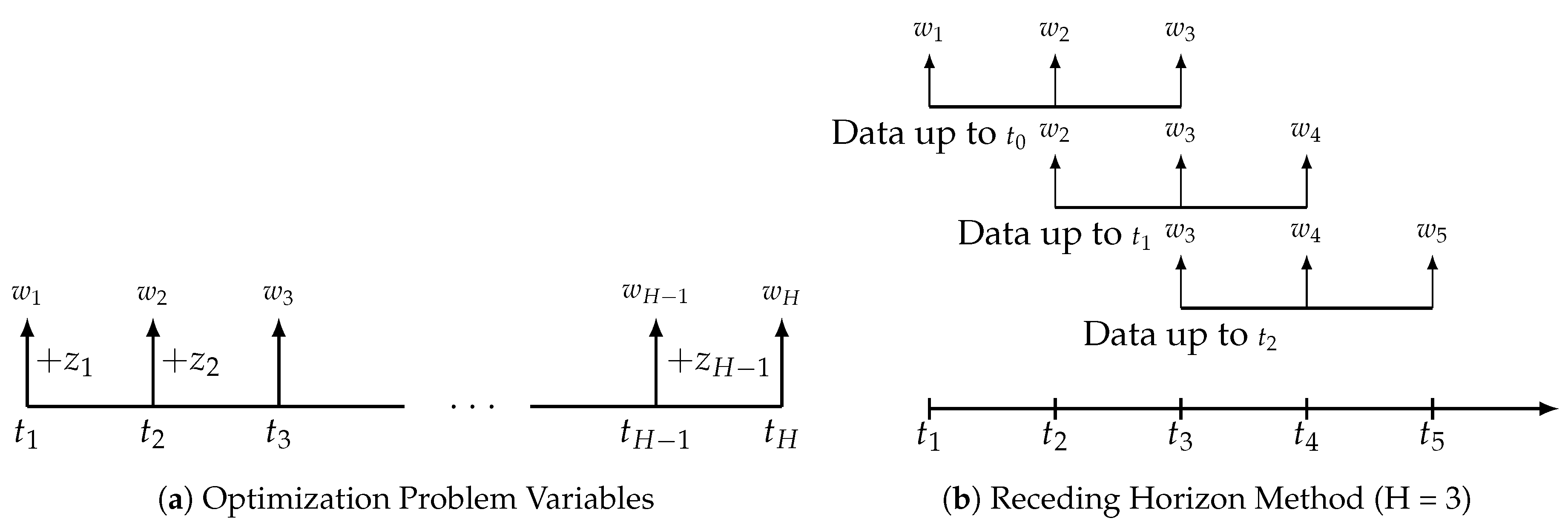
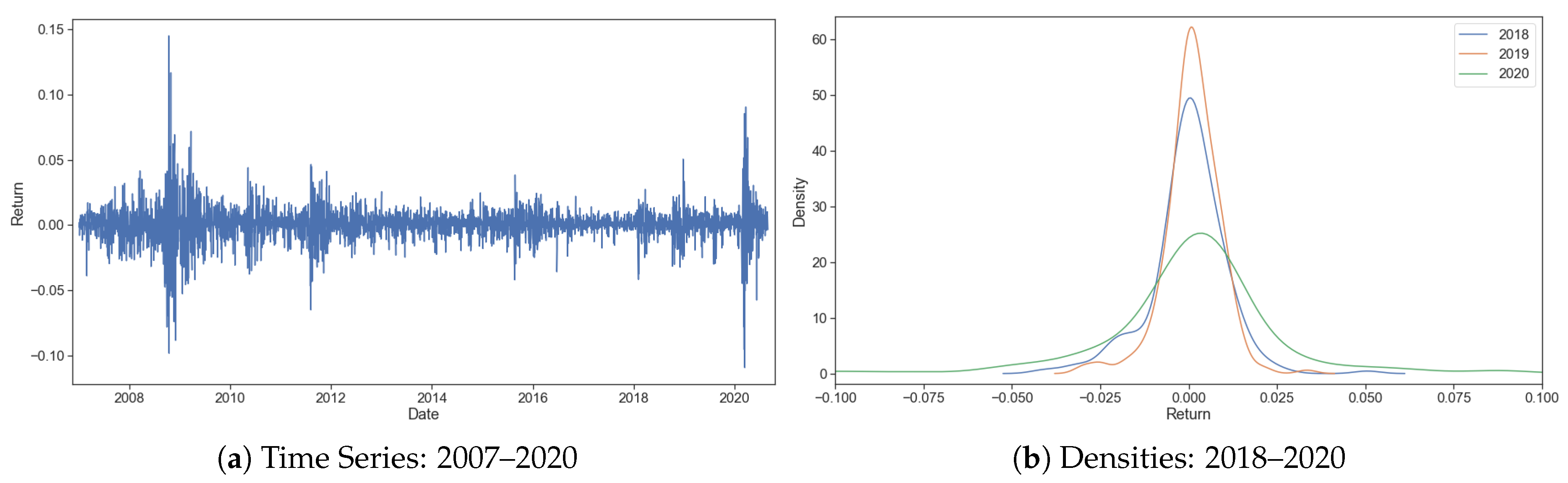
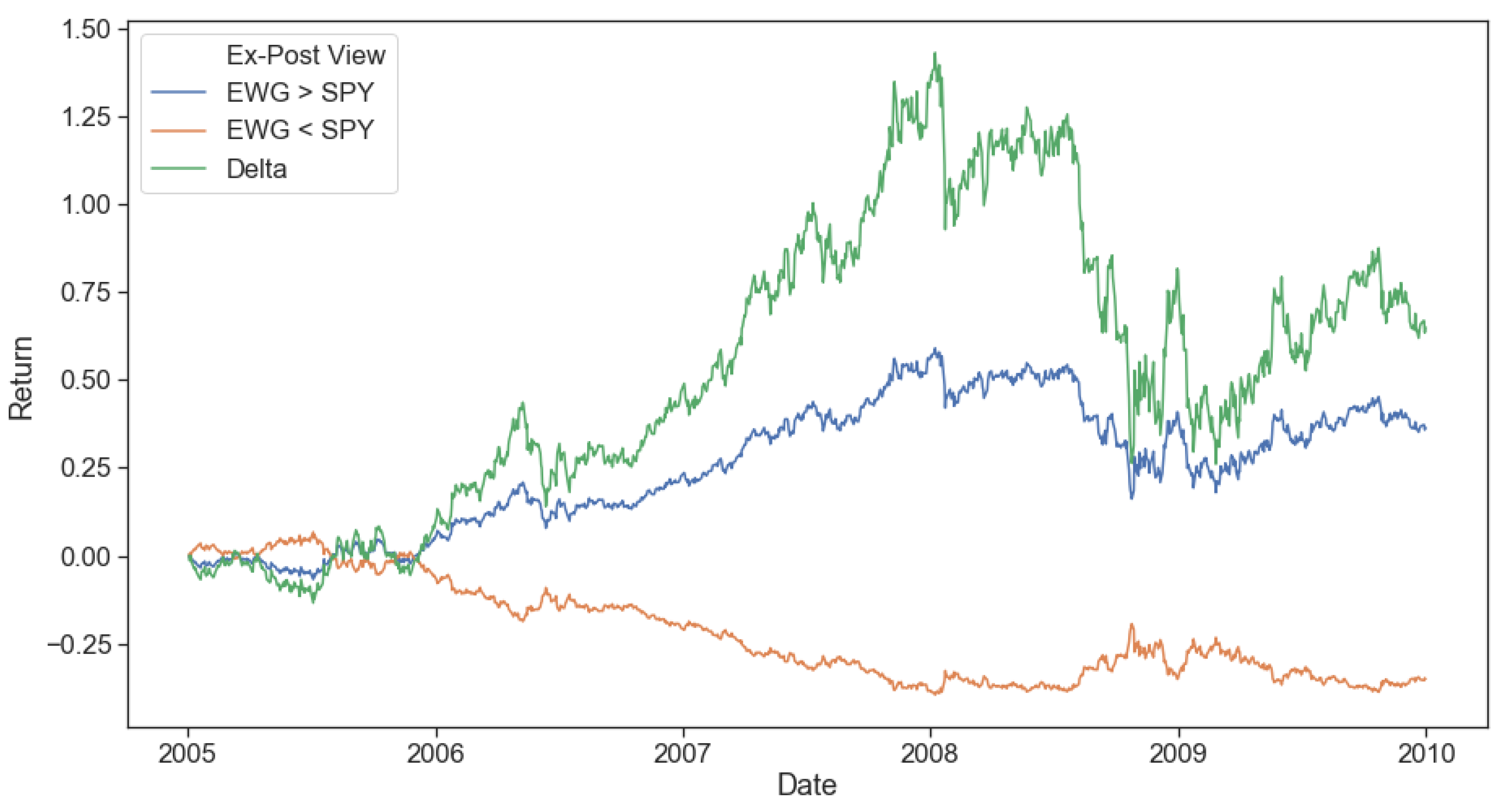
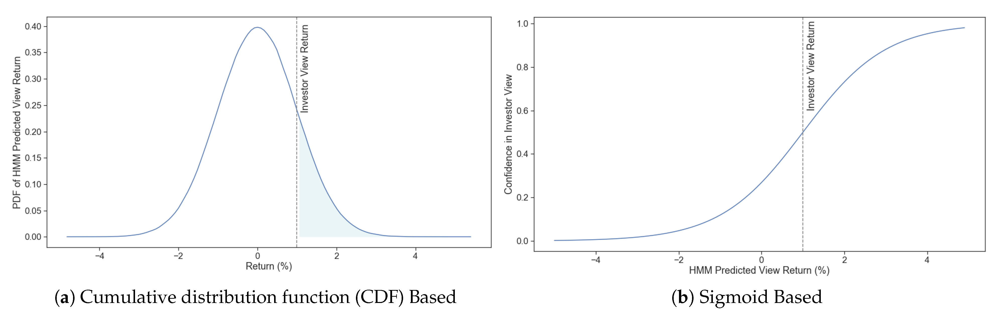
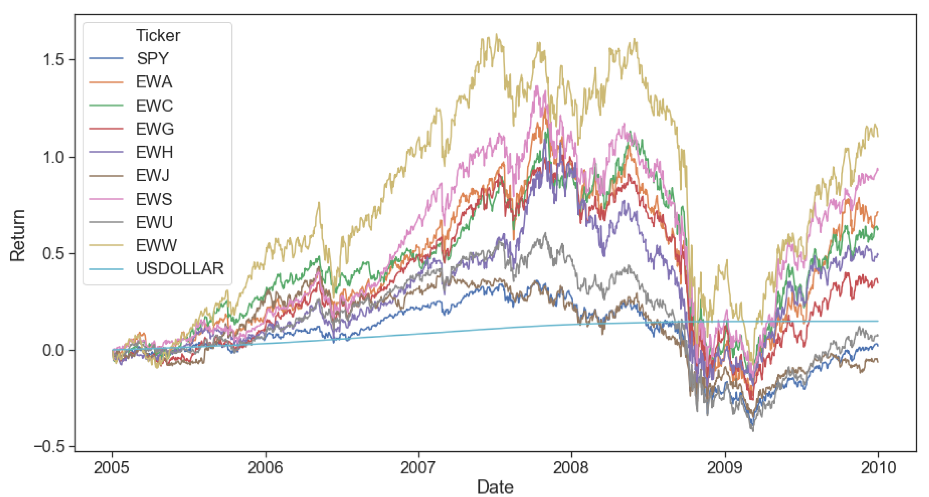
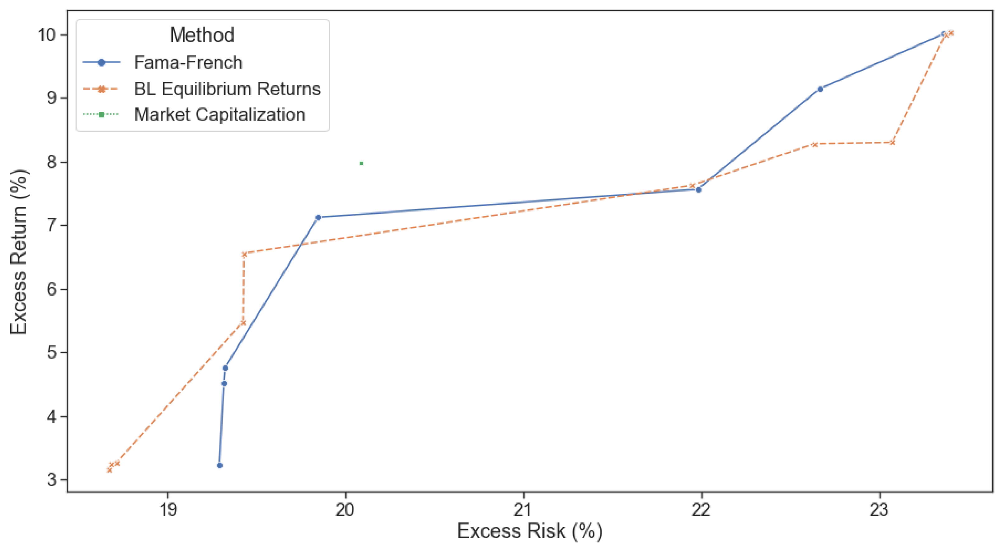
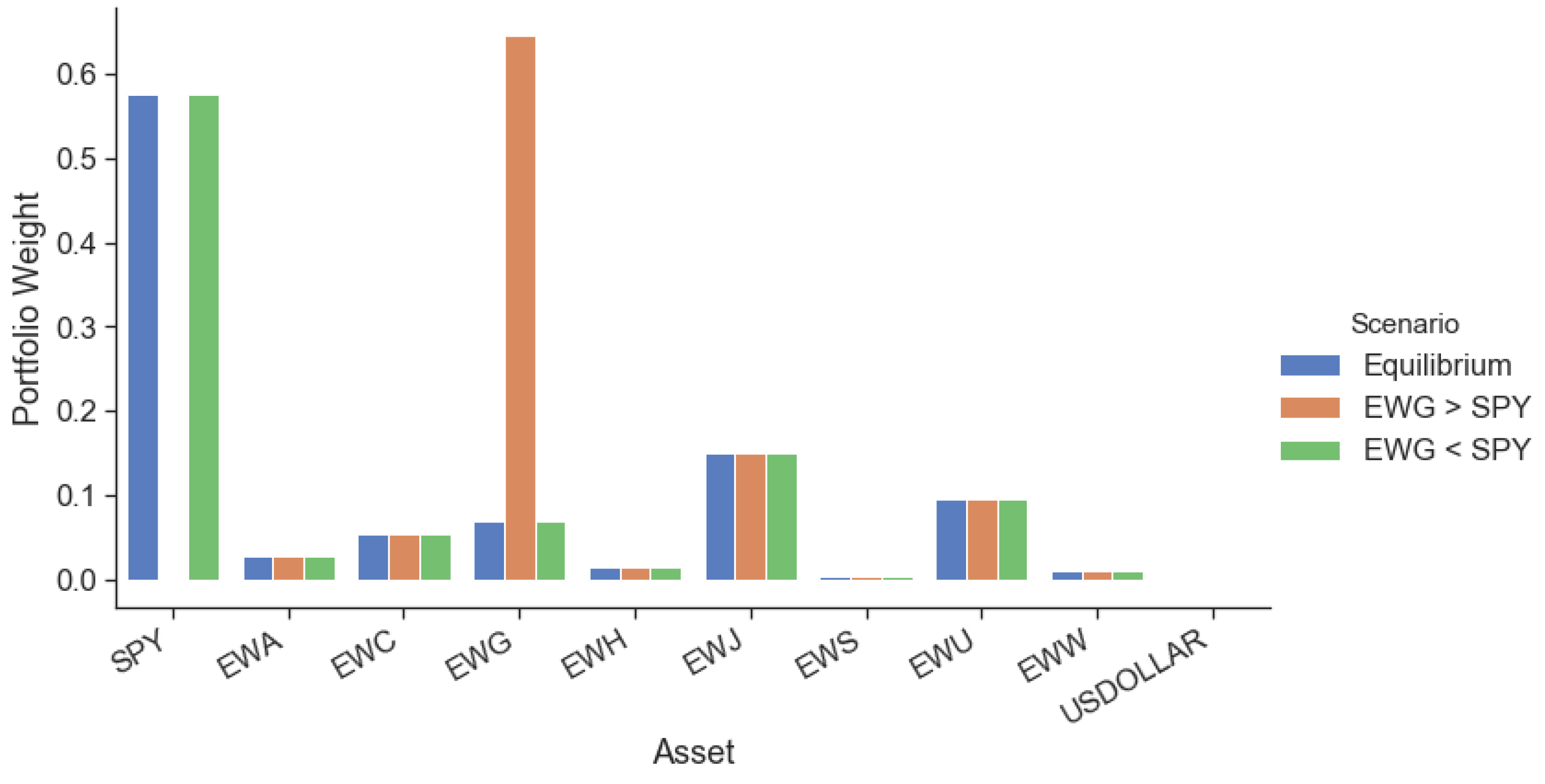
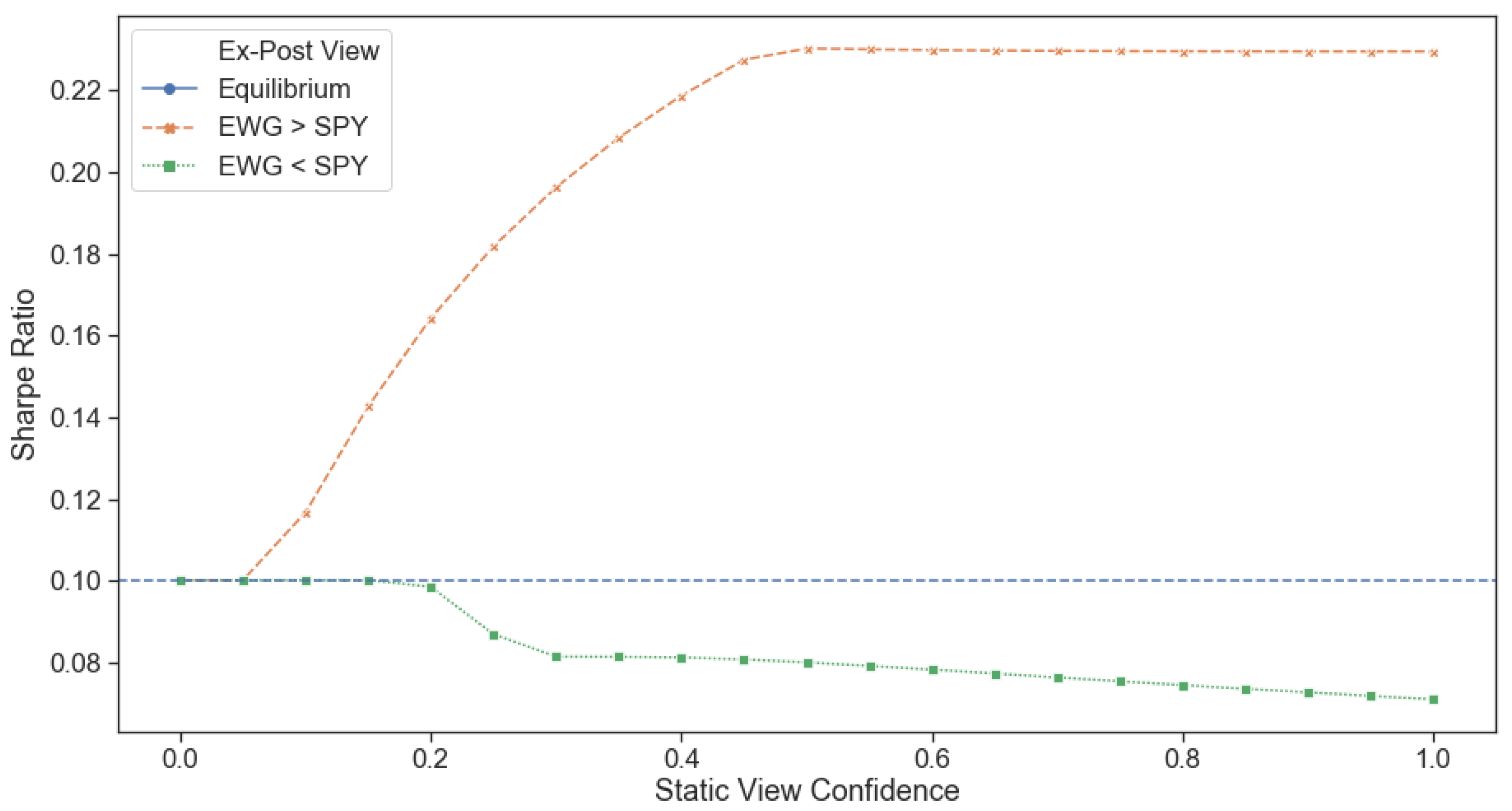
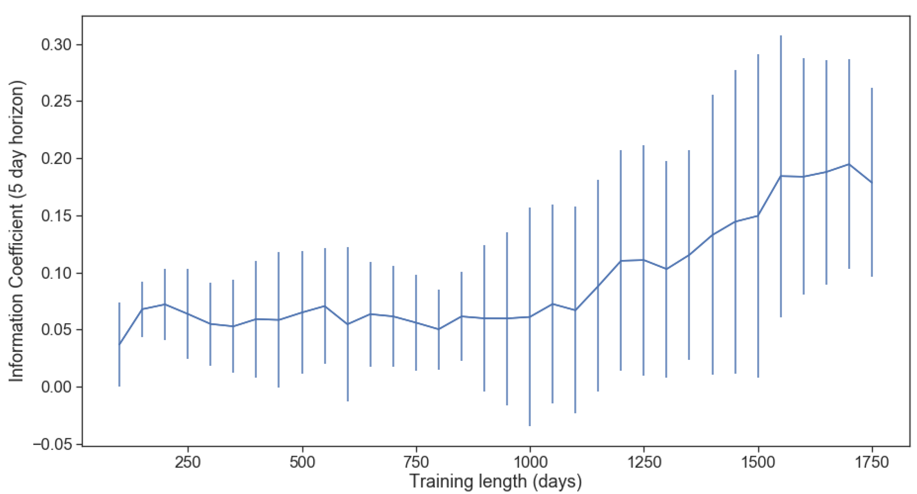
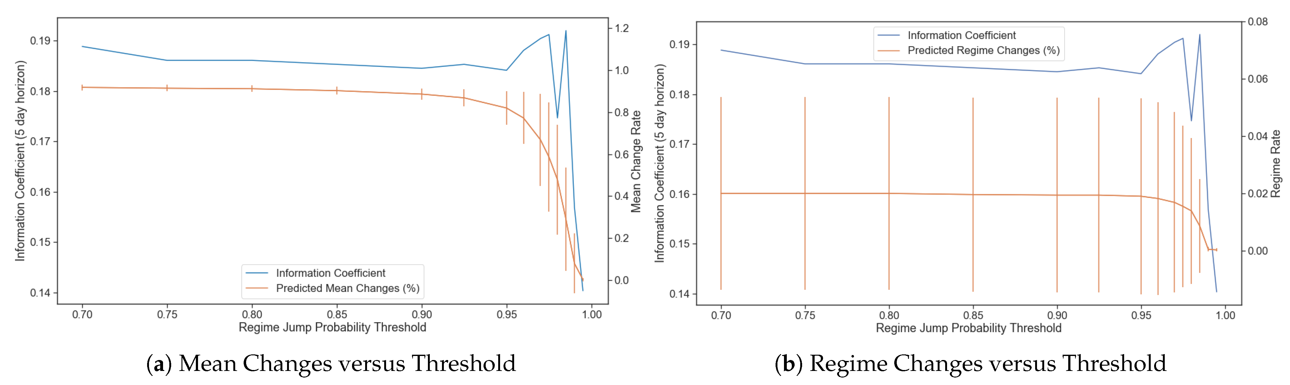
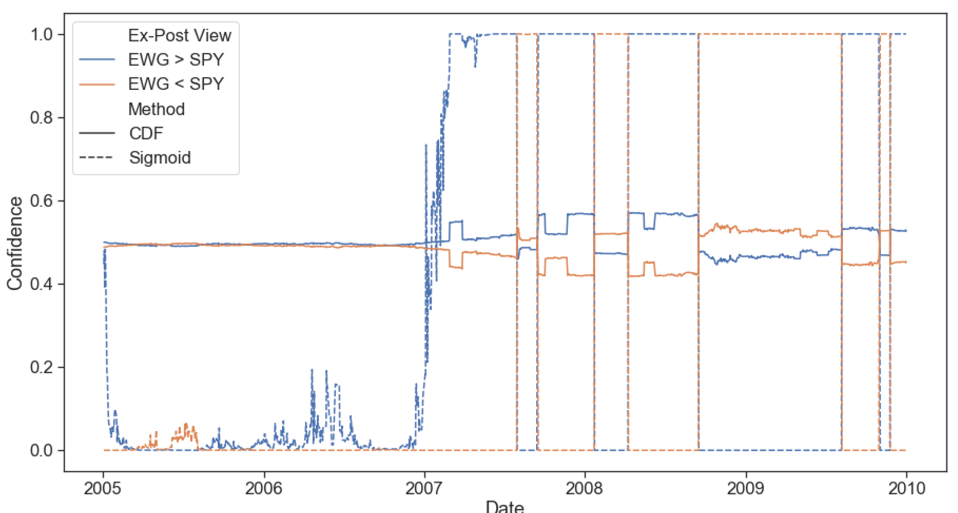
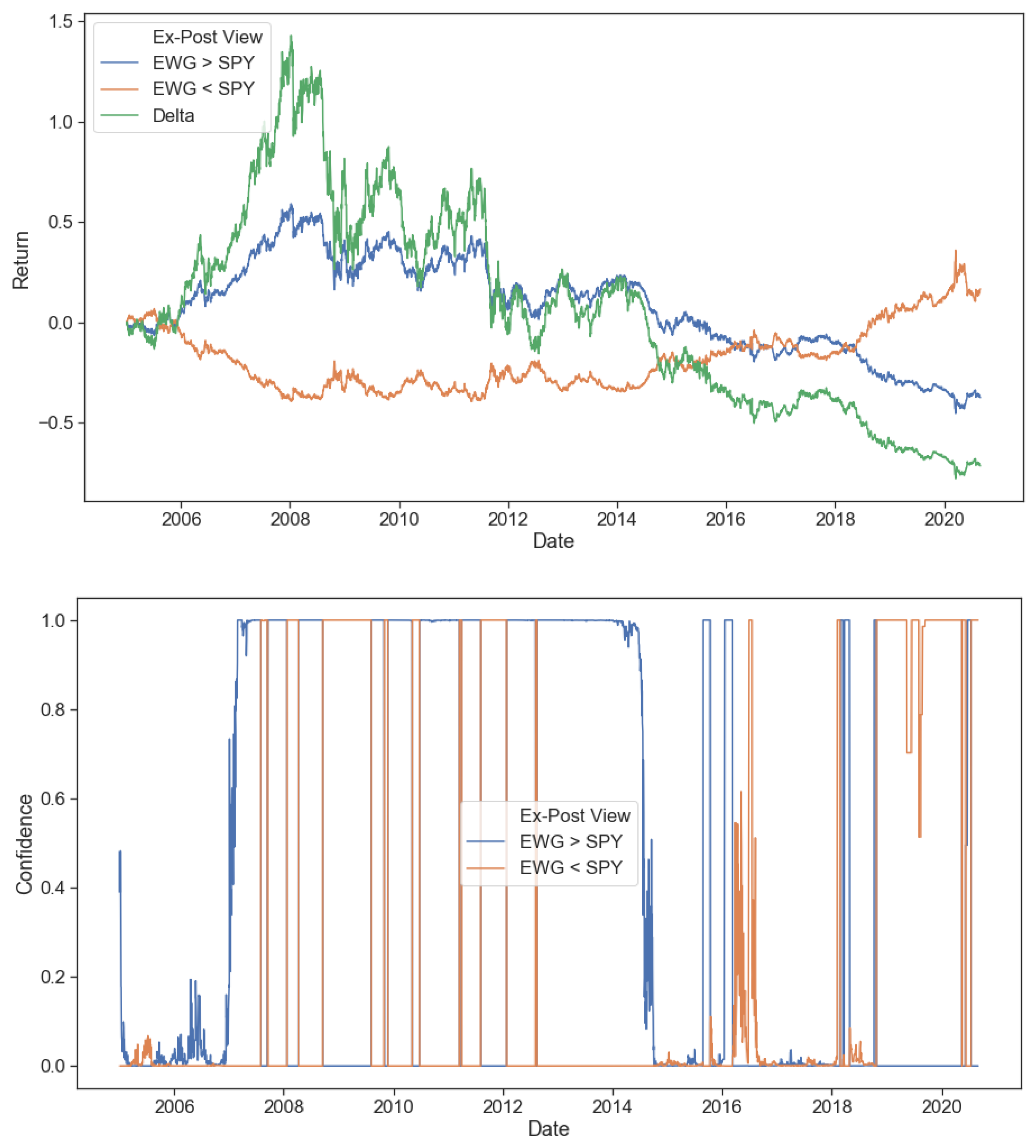
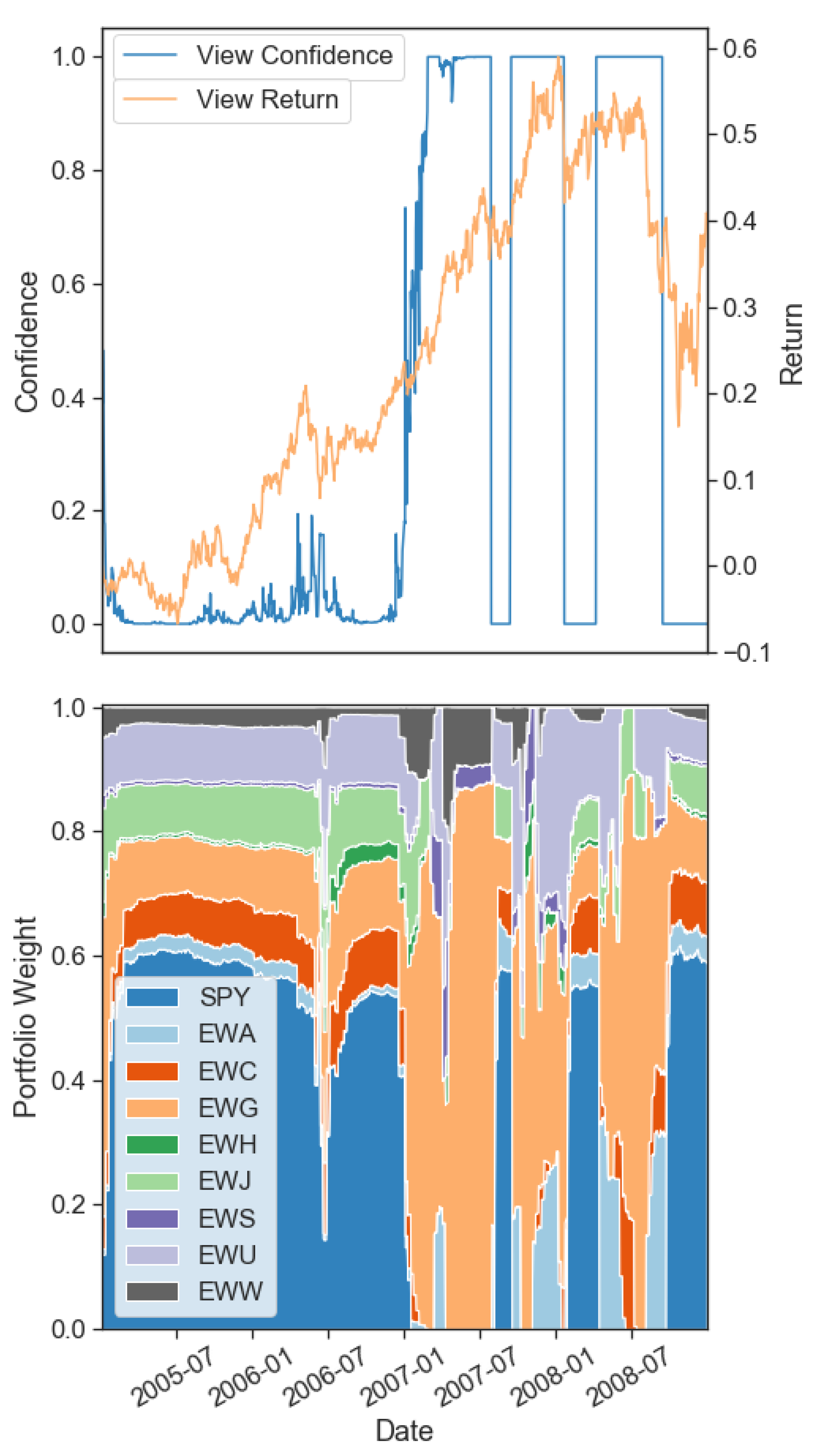
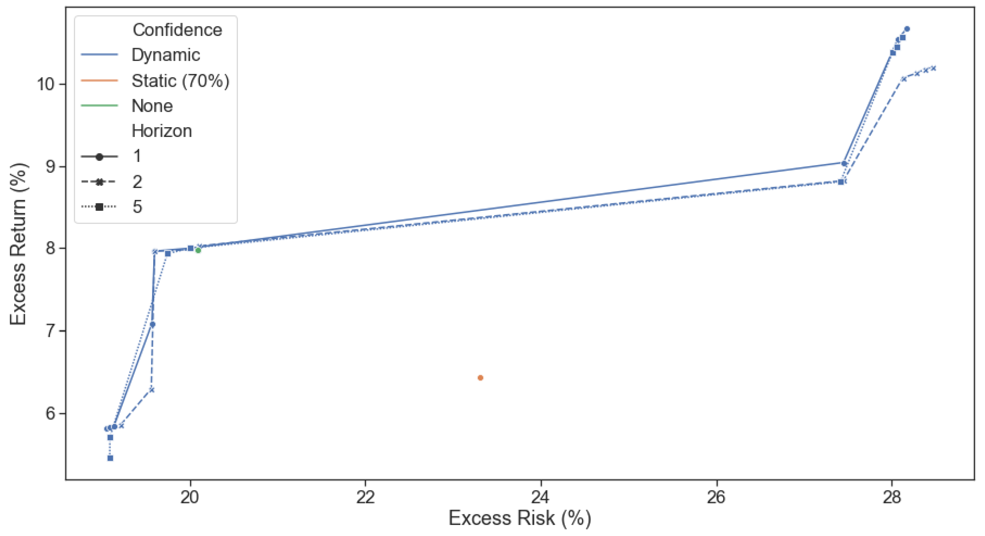
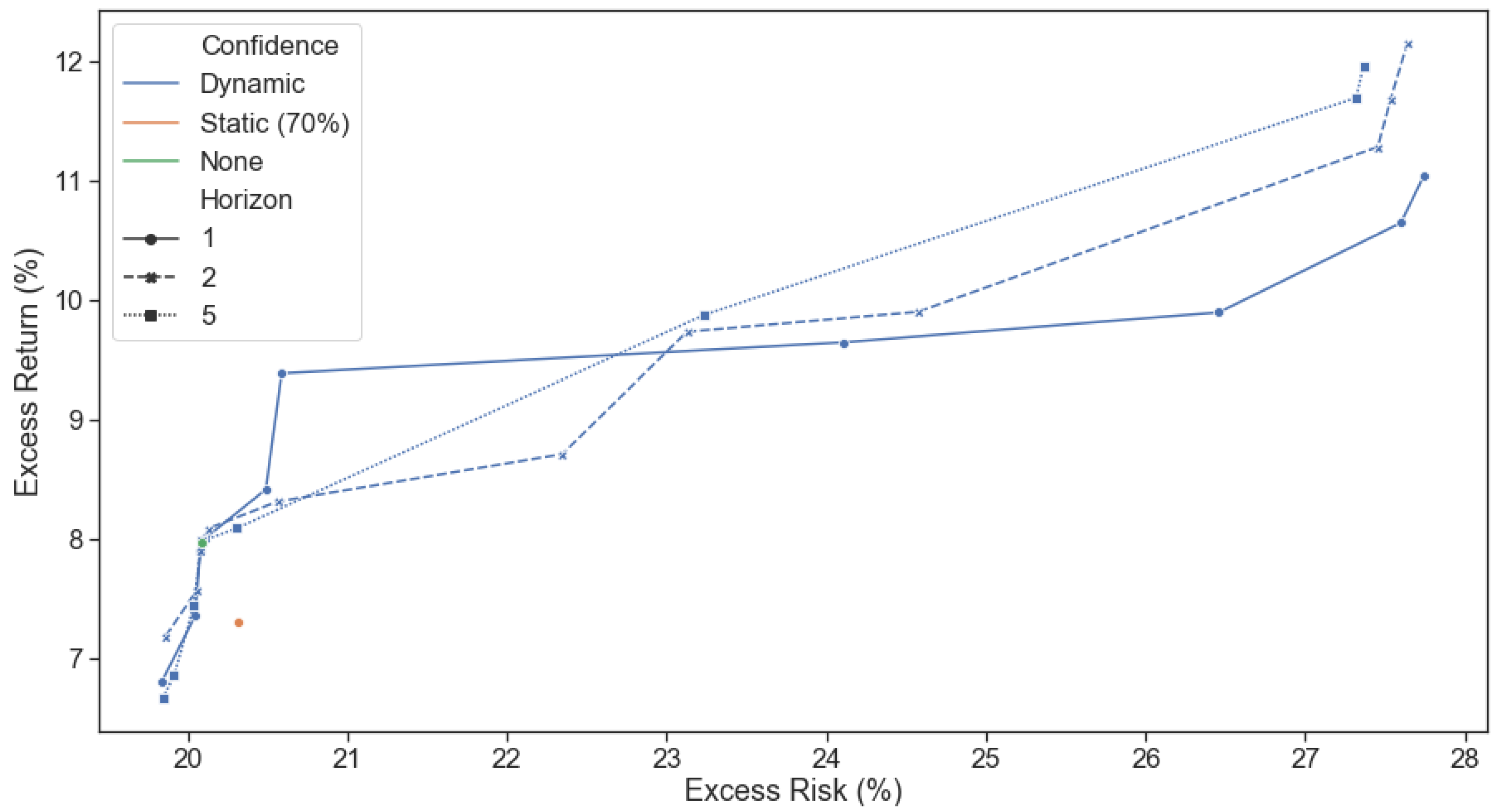
Table 1.
Equity Universe.
| Country/Territory | ETF Ticker | Market Capitalization ($bn) | Equilibrium Weight |
|---|---|---|---|
| United States | SPY | 3179 | 57.6% |
| Japan | EWJ | 830 | 15.0% |
| United Kingdom | EWU | 528 | 9.6% |
| Germany | EWG | 384 | 7.0% |
| Canada | EWC | 239 | 5.4% |
| Australia | EWA | 150 | 2.7% |
| Hong Kong | EWH | 79 | 1.4% |
| Mexico | EWW | 49 | 0.9% |
| Singapore | EWS | 20 | 0.3% |
Table 2.
Performance of Static Confidence (2005–2020).
| Ex-Post View | Excess Return | Excess Risk | Maximum Drawdown |
|---|---|---|---|
| Equilibrium | 7.98% | 20.09% | 57.10% |
| EWG > SPY | 6.43% | 23.31% | 61.64% |
| EWG < SPY | 7.91% | 20.32% | 57.61% |
Publisher’s Note: MDPI stays neutral with regard to jurisdictional claims in published maps and institutional affiliations. |
© 2020 by the authors. Licensee MDPI, Basel, Switzerland. This article is an open access article distributed under the terms and conditions of the Creative Commons Attribution (CC BY) license (http://creativecommons.org/licenses/by/4.0/).
Share and Cite
MDPI and ACS Style
Oprisor, R.; Kwon, R. Multi-Period Portfolio Optimization with Investor Views under Regime Switching. J. Risk Financial Manag. 2021, 14, 3. https://doi.org/10.3390/jrfm14010003
AMA Style
Oprisor R, Kwon R. Multi-Period Portfolio Optimization with Investor Views under Regime Switching. Journal of Risk and Financial Management. 2021; 14(1):3. https://doi.org/10.3390/jrfm14010003
Chicago/Turabian StyleOprisor, Razvan, and Roy Kwon. 2021. "Multi-Period Portfolio Optimization with Investor Views under Regime Switching" Journal of Risk and Financial Management 14, no. 1: 3. https://doi.org/10.3390/jrfm14010003