

Frequency-Resolved High-Frequency Broadband Measurement of Acoustic Longitudinal Waves by Laser-Based Excitation and Detection


Institute of Sensor and Actuator Technology, Coburg University of Applied Sciences and Arts, Am Hofbräuhaus 1b, 96450 Coburg, Germany
*
Author to whom correspondence should be addressed.
Sensors 2024, 24(5), 1630; https://doi.org/10.3390/s24051630
Submission received: 6 February 2024
/
Revised: 27 February 2024
/
Accepted: 29 February 2024
/
Published: 1 March 2024
(This article belongs to the Special Issue Acoustic and Ultrasonic Sensing Technology in Non-destructive Testing)
Abstract
:Optoacoustics is a metrology widely used for material characterisation. In this study, a measurement setup for the selective determination of the frequency-resolved phase velocities and attenuations of longitudinal waves over a wide frequency range (3–55 ) is presented. The ultrasonic waves in this setup were excited by a pulsed laser within an absorption layer in the thermoelastic regime and directed through a layer of water onto a sample. The acoustic waves were detected using a self-built adaptive interferometer with a photorefractive crystal. The instrument transmits compression waves only, is low-contact, non-destructive, and has a sample-independent excitation. The limitations of the approach were studied both by simulation and experiments to determine how the frequency range and precision can be improved. It was shown that measurements are possible for all investigated materials (silicon, silicone, aluminium, and water) and that the relative error for the phase velocity is less than 0.2%.
1. Introduction
In industry and academic research, optoacoustics has already been established in many applications [1]. The advantages of this method is the fact that the measurements are non-destructive and non-contact [1,2,3]. It should also be emphasised that photoacoustic measurements are very broadband due to laser excitation, which means that frequency-dependent analyses can be carried out in a range from to [4]. This allows macrostructures and thin films, as well as microstructures, to be probed [1]. Photoacoustics is, therefore, a promising technique for the study and analysis of complex media properties [3].
Bulk acoustic waves are typically non-dispersive, and measurements are performed with a single frequency or in a narrow frequency band. The recent literature has shown that the dispersion of bulk acoustic waves can be utilised to measure material properties such as material inhomogeneity. Karabutov et al. [5] presented a method that allows conclusions about the porosity of isotropic metal matrix composites from the dispersion of the phase velocity and the frequency-resolved attenuation of longitudinal waves. Podymova et al. [6] have demonstrated that the effect of porosity on the dispersion of longitudinal waves is also present in aluminium alloy matrix composites. Other researchers have characterised 3D-printed photopolymers by measuring frequency-resolved acoustic properties [7,8]. The dispersion of longitudinal waves inside of Polyvinylchloride (PVC) has been shown by Demcenko et al. [9].
In addition, during the development and testing of acoustic metamaterials, a frequency-resolved broadband characterisation of materials is necessary. Examples of metamaterials with dispersive longitudinal waves can be found in the literature [10,11,12]. Thus, broadband, frequency-resolved measurements of sound velocity and attenuation open up new possibilities for materials analysis.
One method of broadband excitation of acoustic waves is excitation via a nanosecond pulsed laser. This excitation method enables non-destructive and non-contact measurements with a broad frequency spectrum and high amplitude signals [13,14]. This excitation technique for short ultrasonic pulses is used for the excitation of longitudinal [15,16,17], shear [18,19,20], Rayleigh [21,22,23,24,25], and lamb waves [26,27,28,29]. All studies require high-quality experimental data and a deep understanding of the limitations of the experiment and the analysis.
In this paper, we present an optical method for precise, low-contact, non-destructive, sample-independent, broadband, and frequency-resolved measurement of the dispersion and attenuation of compression waves. The components of the measurement setup are introduced, and their purpose and impact on the measurement are discussed. Simulations and experiments were used to identify factors influencing the generation of sound by a pulsed laser. Further experiments were performed to analyse the accuracy of the method.
In the following section, we first introduce the idea of the measurement method and explain the components, starting with detection and going backwards to excitation. Special attention is paid to the measuring cell, its components, and its influence on the measurement. The influence on the measurement is first demonstrated using simulations and, later, using experimental measurements. The article concludes with dispersion measurements of various materials.
2. Materials and Methods
2.1. Concept of the Measurement Setup
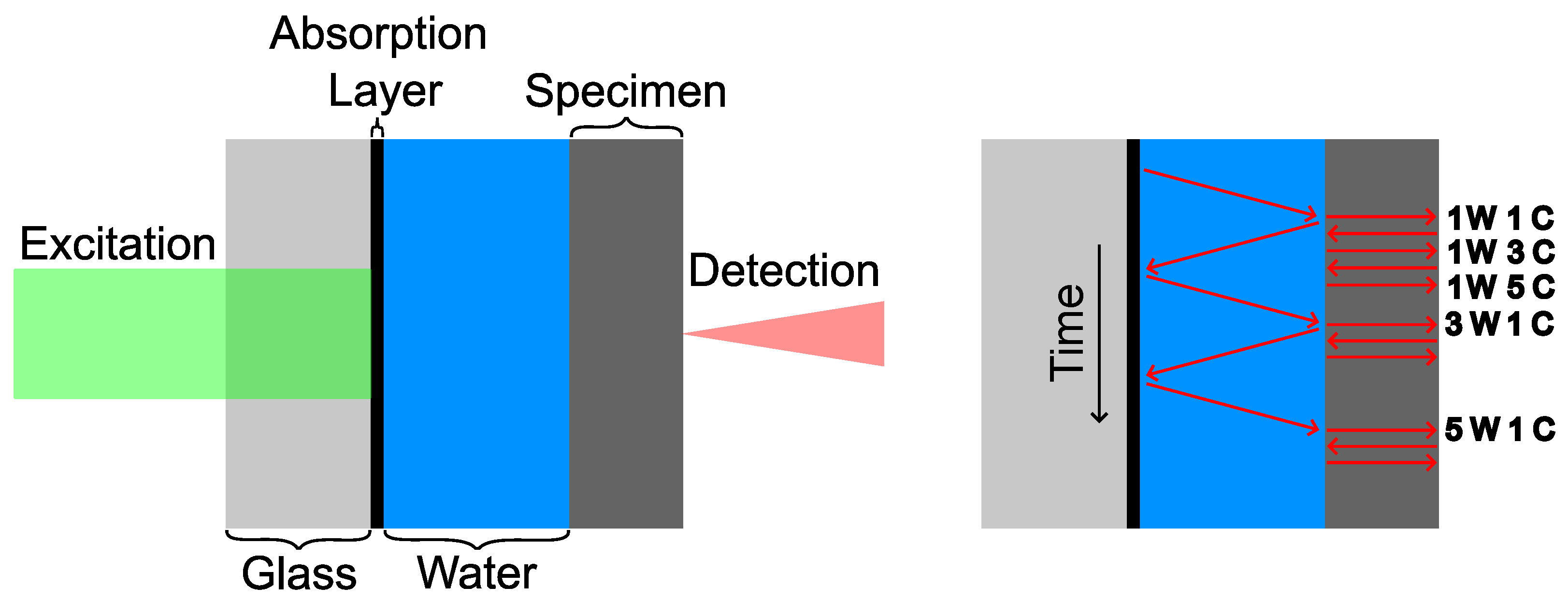
The acoustic measurement cell is the centrepiece of the measurement setup. It consists of an absorption layer on top of a glass substrate, the specimen, and water in contact with the absorption layer and the specimen. There are several objectives that are addressed with the measuring cell presented below (see Figure 1):
- The measurement of the frequency-resolved phase velocity and attenuation of acoustic compression waves.
- The excitation and detection of an acoustic compression pulse independent of the sample material and over a wide frequency range.
- Non-destructive and ideally contactless measurement.
- The suppression of other acoustic excitations, e.g., shear waves.
Figure 1.
Scheme of acoustic measurement cell. (Left) Components of measurement cell. (Right) Scheme of possible acoustic paths. C: Path of compression wave through specimen. W: Path of compression wave through water. Time axis is not scaled.
Figure 1.
Scheme of acoustic measurement cell. (Left) Components of measurement cell. (Right) Scheme of possible acoustic paths. C: Path of compression wave through specimen. W: Path of compression wave through water. Time axis is not scaled.

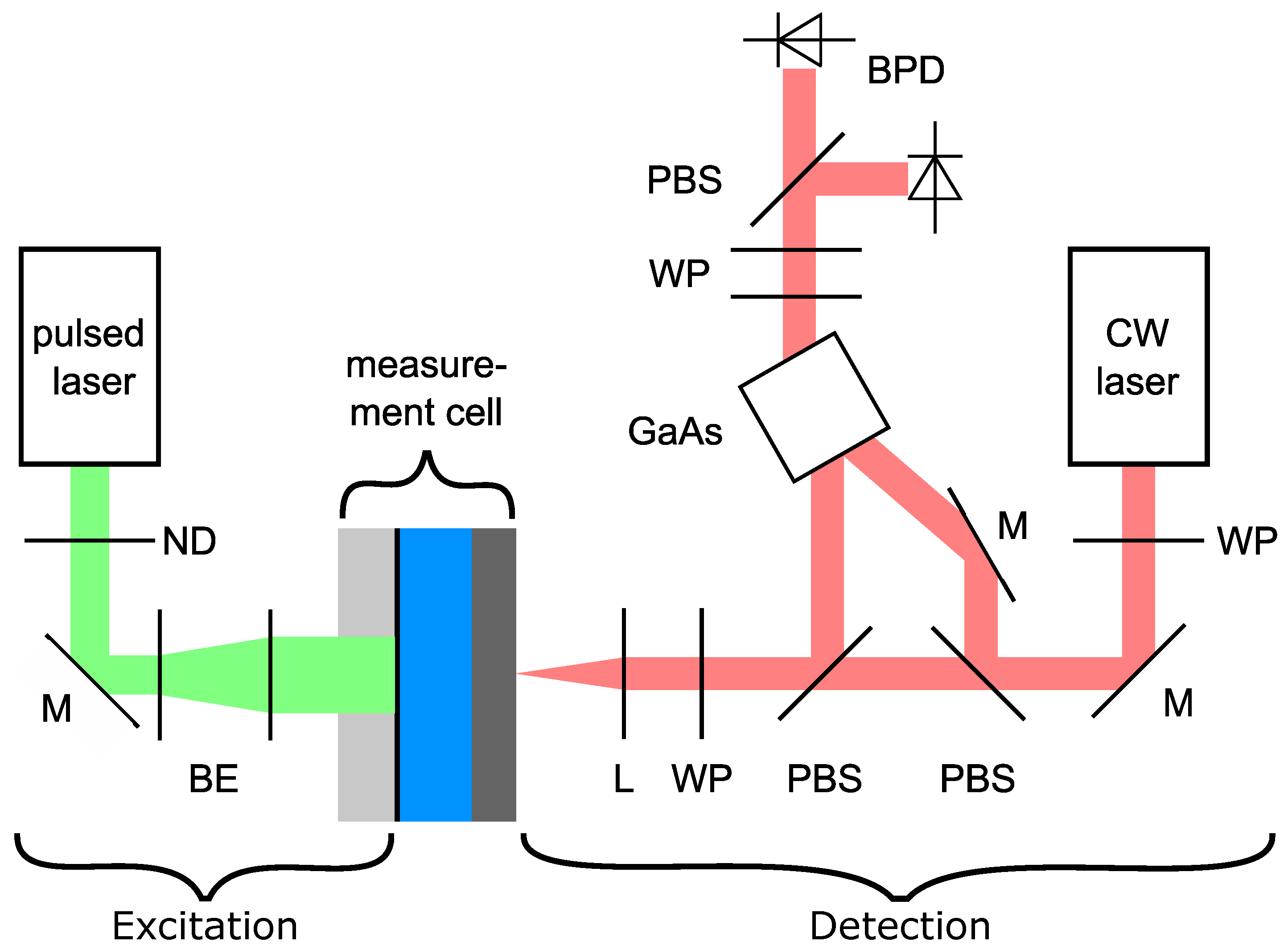
The ultrasonic pulse is generated at the absorption layer via an ns pulsed laser. From this layer, the pulse travels through the water and the specimen and will be detected with an adaptive interferometer with a photorefractive crystal. The complete optical setup is visualised in Figure 2.
In the following section, we discuss the individual components, their purpose, and their influence on the measurement, starting at detection and going backwards to excitation.
2.2. Detection
The ultrasonic waves were detected using a self-built adaptive interferometer with a photorefractive crystal. These interferometers, used for the detection of ultrasonic waves or vibrations, are well described in the literature [30,31,32]. In our setup, we used an undoped GaAs crystal (5 × 5 × 10 ) in a diffusion-dominated regime with an anisotropic diffraction setup. The optical setup for the detection is shown in Figure 2.
This kind of interferometer has several advantages. The wavefront of the diffracted beam is identical to the wavefront of the nondiffracted beam of the sample beam, allowing both beams to interfere with exactly the same wavefronts [30,33]. A possible source of wavefront distortion can be, for example, the surface roughness of the sample. The dynamic hologram inside the crystal acts as a high-pass filter with a cut-off frequency with a time constant of the crystal (). The cut-off frequency depends on the setup and is in the range of 3.5 and 10 for GaAs crystals [30]. The high-pass suppresses low-frequency disturbances, such as air fluctuations, thermal deformation, acoustic noise, and other sources of vibration [30,33]. In addition the interferometer has a wide frequency response [33], with a flat transfer function above its cut-off frequency and below the bandwidth of the balanced photodetector [32,34].
Detection is the main component, which defines the noise level of the setup. The noise level is mainly determined by the laser power of the interferometer, the number of averages, the detector, and the electronic and acoustic background noise.
In our setup, we used a 1064 laser with a maximum CW power of 10 (Azurlight Fiber Laser, Azurlight Systems, Bordeaux, France), operating at 3 , and an InGaAs photodetector (Femto HBPR-200M-30K-IN, FEMTO Messtechnik GmbH, Berlin, Germany), with a bandwidth of DC up to 200 .
2.3. Measurement Cell
This section describes the individual components of the measuring cell (see Figure 1) and their influence on the measurement.
2.3.1. Specimen
The measuring cell was designed in such a way that the measurement is as sample-independent as possible.
It is only necessary for the evaluation (see Section 2.4.1) that two reflections of the same pulse (e.g., 1W 1C (the pulse travels one time through the water and the compression wave travels one time through the sample) and 1W 3C, as compared in Figure 1) can be measured. This sets the requirements for the sample in terms of acoustic attenuation and thickness.
2.3.2. Fluid
The sound pulse is transmitted through the liquid to the sample. Only longitudinal waves can propagate in the liquid, which means that primarily longitudinal waves can be observed in the sample.
A further task of the fluid is to delay the reflection of the wave at the absorption layer (3W 1C, as compared in Figure 1) so that at least a number of reflections can be measured within the sample before the first interfering reflection occurs. This delay can be adjusted by the fluid thickness and its velocity .
where and are the thickness and acoustic velocity of the sample, and is the acoustic pulse duration. The first term of the equation describes that reflections can be measured before the wave propagating in the fluid is detected for the first time. The second term ensures that the two waves do not overlap due to the pulse duration.
Considering the acoustic attenuation in the fluid, the aim should be to minimise the fluid thickness while still fulfilling the condition above. The literature typically describes the frequency-dependent attenuation by a power law [35,36]. For water, a quadratic dependence on frequency is commonly assumed [35,37,38,39,40,41,42].
The literature often provides values for k in the range of , measured for frequencies up to 15 [37,39,40,41]. Other sources give slightly higher attenuations of 0.4 to 1 [43] or [44] up to very high values of 44 [36]. Sometimes, a linear dependence is also assumed with values from [45] to 30 [46].
The reflection and transmission factor and, therefore, the acoustic impedance difference at the fluid–sample interface influence the signal strength of the different reflections inside the sample. On the one hand, a low reflection coefficient is good for the transmission of the acoustic wave from the fluid into the sample, and on the other hand, a high reflection coefficient is good for additional reflections within the sample. Neglecting the transmission between the sample and the surrounding air, the optimal reflection coefficient for the reflection inside the sample is
This fact must be considered when selecting the liquid. The choice of liquid can be influenced by other factors, such as potentially hazardous substances, solvent vapours, and the material compatibility of the sample with the liquid. Equally important is the cleaning effort required to remove the liquid from the cell and the sample.
We used deionised water and hydraulic oil in our setup. Unless stated otherwise, the fluid layer was water and 9 thick.
2.3.3. Absorption Layer
The absorption layer is the main part that influences the generation of acoustic waves. Excitation via an absorption layer has two advantages. Firstly, the material of the absorption layer can be freely chosen. Secondly, the excitation of the acoustic wave is independent of the sample.
The absorption layer should not be damaged; therefore, the excitation had to be selected to be in the thermoelastic regime (see Section 2.3.5). The damage threshold of the absorption layer defines the maximum pulse energy of the laser (Equation (7)).
The acoustic impedance of the absorption layer should match the impedance of the fluid to enable good transmission of the acoustic pulse into the fluid.
In Section 3.1, we simulated the influence of different material properties on the elongation and frequency spectra of the excited acoustic pulse (see Formulas (19)–(21)). The elongation of the pulse increases with the thermal expansion coefficient while decreasing with the density, specific heat capacity, Young’s modulus, and optical absorption coefficient. The material parameters of polymer-based materials, with the exception of specific heat capacity and absorption coefficient, result in higher acoustic amplitudes compared to metal-based materials. Polymer-based materials also fulfil the impedance condition mentioned above better than metallic materials.
To achieve measurements with a high bandwidth, the decrease in the frequency spectrum should be small. According to the simulations (see Formula (20)), a high acoustic velocity and high optical absorption are advantageous. The desired slow decrease in the frequency spectrum is, therefore, inverse to the elongation in terms of the density and optical absorption coefficient. The frequency spectra (see Appendix A) show that the increasing power compensates for the stronger drop at high frequencies. Polymer-like materials are, therefore, preferable.
Another aspect to consider is the thickness of the absorber. If the absorber is slightly transparent, an acoustic pulse will be generated at the glass–absorption layer interface and the absorption layer–fluid interface. The influence of reflections within the absorption layer can be minimised by a layer that is as thin as possible.
We used two kinds of absorption layers. The aim of the first coating was to obtain a thin layer and a small slope in the frequency spectrum. A sputtering process was chosen for this purpose. Based on the absorption coefficient at the excitation wavelength, the coefficient of thermal expansion, the specific heat capacity, and the density, chromium was chosen for the absorption layer. The thickness was 125 .
The aim of the second layer was to excite waves with high amplitudes. Polydimethylsiloxane (PDMS) was chosen because of its very high coefficient of thermal expansion, low density, and low elastic modulus compared to metals. Carbon was added to the PDMS to increase optical absorption. The spin-coated layer was approximately 50 thick.
2.3.4. Glass
A glass substrate has several functions. It acts as a support for the absorption layer and also as a constraining layer (see Section 2.3.5). A constraining layer increases the amplitude of the generated acoustic pulse. The glass needs to be transparent for the wavelength of the pulsed laser. The glass substrate must have a minimum thickness so that the reflection at the rear end of the substrate is sufficiently delayed until the wave reaches the detector position.
As discussed earlier, we want a minimum of pulses inside the sample before the first unwanted signal occurs. This results in a minimum glass thickness of
where and are the longitudinal velocity inside the glass and sample, respectively; is the thickness of the sample; and is the acoustic pulse duration. The signal strength is also positively influenced by a high reflection factor between the glass and the absorption layer. A high impedance difference should be aimed for.
where and are the acoustic impedance of the glass and the absorption layer.
2.3.5. Excitation
For laser excitation, there are several points to consider: the excitation regime, the excitation spot size, the laser wavelength, and the pulse duration.
There are two regimes for laser excitation of ultrasonic waves. The first is thermoelastic excitation, which is truly non-destructive because the absorbed laser pulse is below the damage threshold of the material [15]. The second regime is ablative excitation, which is destructive because the laser pulse energy is above the damage threshold and vaporises the material [15].
Aussel et al. [47] show that material evaporation due to excessively absorbed power densities occurs under the following condition:
where is the thermal conductivity, is the density, is the specific heat capacity, is the laser pulse duration, is the vaporisation temperature, and is the initial temperature.
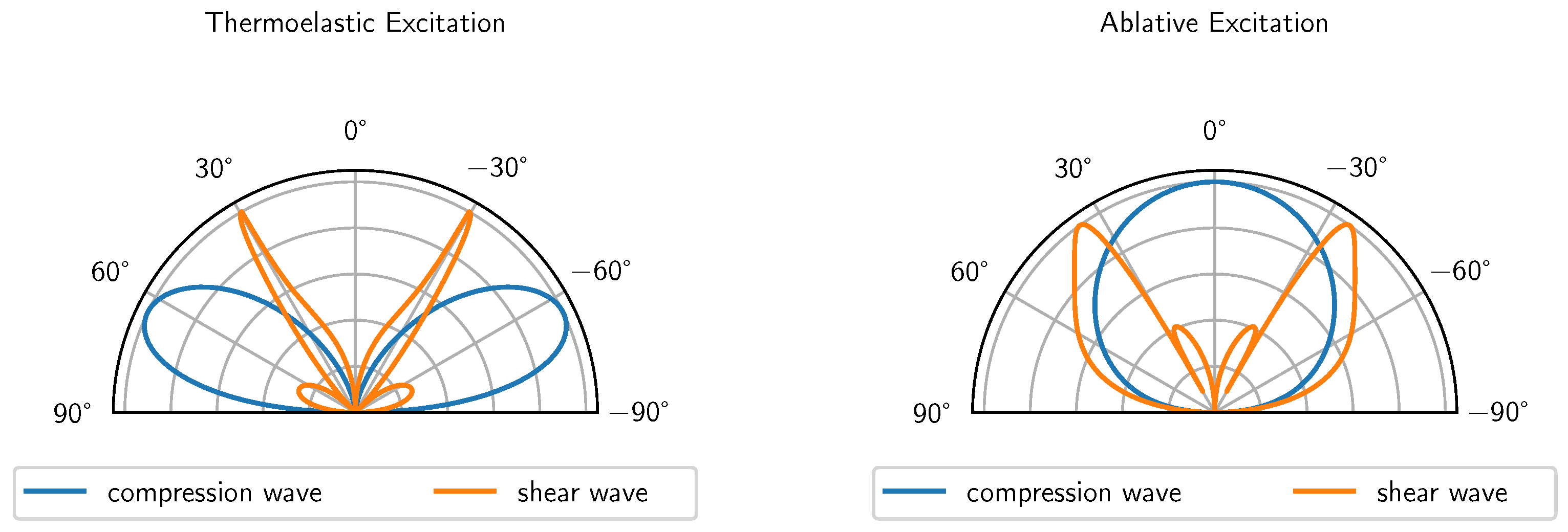
For a point laser source, the excited waves under a propagation angle can be described by analytical formulas [13].
For the thermoelastic excitation of a point source [13]:
And, for the ablative excitation of a point source [13]:
where the wavevector . The index c represents the compression wave, and the index s represents the shear wave. The analytical formulas are visualised in Figure 3 for aluminium.
The measuring cell presented in this paper is based on compression waves that propagate in a normal direction. Therefore, a point source in the thermoelastic excitation regime is not suitable due to the directivity of the compression waves (see Figure 3 (left)). Ablative excitation has a suitable radiation characteristic but cannot be used because of the minor surface damage it causes, which would damage the thin absorption layer.
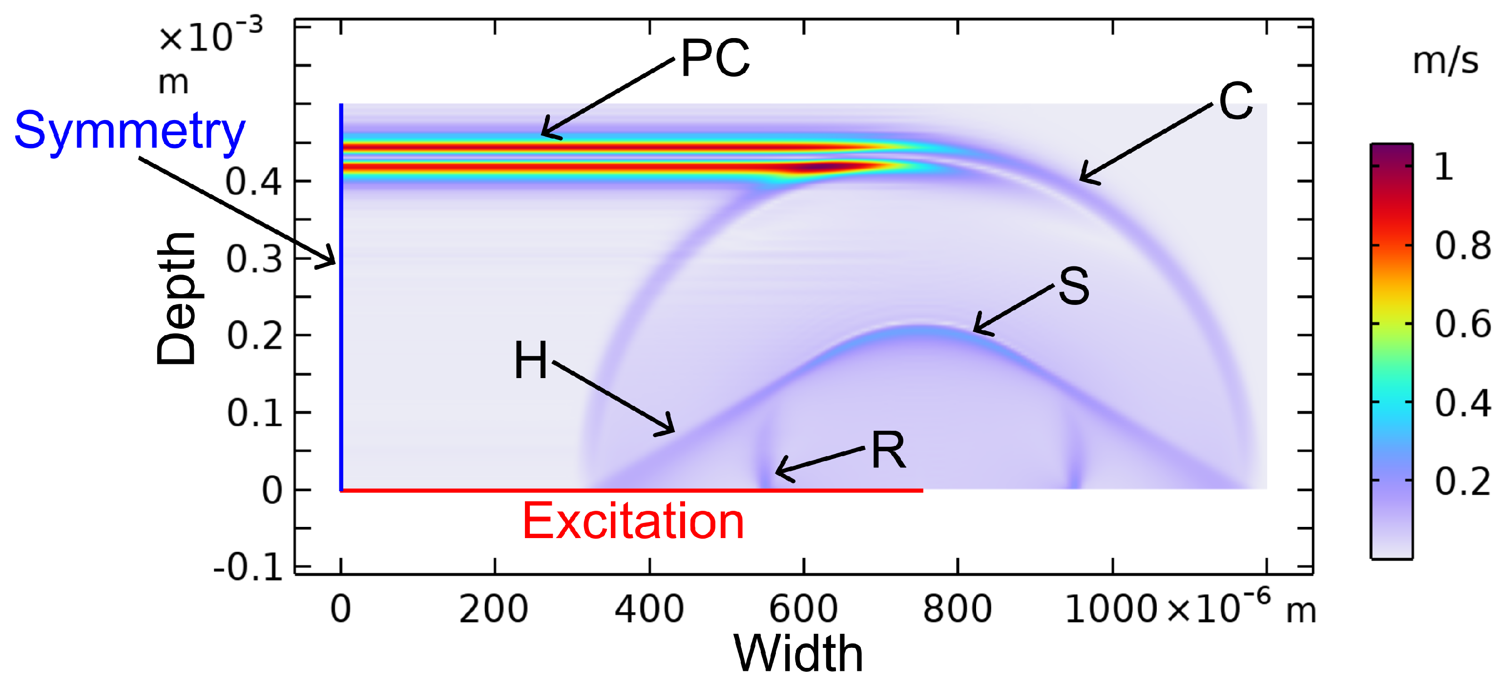
Since the use of point sources is not advantageous in our case, extended sources were investigated. The excited waves using extended sources can be calculated using FEM. In our case, we used COMSOL 6.1. The propagated waves after 75 are visualised in Figure 4. The extended source results in a plane compression wave (PC) as well as additional waves (head (H), compression (C), shear (S), and Rayleigh (R) waves) at the edge of the excitation [47]. These waves do not contribute to the sensing concept but can interfere with the plane compression waves.
A plane compression wave, whose plane wave front propagates parallel to the excitation, is the desired wave for this application. This plane compression wave is not obtained in point excitation.
In addition, the strength of the excitation amplitude can be increased by using a transparent constraining layer, resulting in a buried ultrasonic source. This enables the generation of normal stresses, resulting in an enhanced generation of compression waves [48]. Hutchins [49] used light oil, silicone resin, water, and acetone as a constraining layer and increased the compression wave amplitude by 21 to 25 dB compared to the unmodified surface. The use of a glass slide, cemented to the surface, increased the amplitude by 30 dB. The use of a buried source is, therefore, advantageous and was used in the experiments. In our case, the glass substrate and the water acted as a constraining layer. Deionised water was used to minimise the interaction with the specimen and reduce the cleaning effort compared to other fluids like oil.
If the measurement is not completely in the near field of the acoustic waves, there are two negative aspects to consider. In the far field, sound energy decreases with distance z by [50], while it remains constant in the near field. In addition, the ultrasonic wave experiences a phase shift of in the transition between near and far field [51,52].
If the waves were measured in the transition area or in the far field, both effects had to be taken into account when calculating the attenuation or phase velocity. The near-field length L can be used as an approximation for the transition between both fields [53,54].
where D represents the excitation diameter, and represents the wavelength of the acoustic wave. High-frequency components are normally in the near field and therefore not affected. The transition to the far field for low-frequency components resulted in a lower cut-off frequency, at which errors occurred.
The laser wavelength was of secondary importance. The laser light should have low absorption in the glass and high absorption in the absorption layer.
Pulse duration influenced the amplitude and frequency spectra of the excited waves. Longer pulses resulted in a higher energy input into the absorption layer and increased the amplitude of the acoustic wave while decreasing the frequency bandwidth (Formulas (20) and (21) and Figure A6). For measurements in the mid to upper double-digit MHz range, a single digit pulse duration of a few nanoseconds was appropriate. Short pulses with high power may damage the sample.
In our experiments, we used a 4 pulsed laser (Brilliant, Quantel-Laser, Les Ulis Cedex, France) at 532 and a pulse energy of about 18 (after some neutral density filter). The beam diameter was chosen to be 18 to ensure diffraction-free propagation of the acoustic beam. A second pulsed laser (Wedge, Bright Solutions, Cura Carpignano, Italy) with a 1 pulse duration, at 532 , and a 1 pulse energy was used to investigate the influence of pulse duration. Due to the low pulse energy, a beam cross-section of 2 was selected for this laser.
2.4. Data Analysis Methods
As mentioned in the introduction, the target quantity is a frequency-resolved measurement of phase velocity and attenuation over a wide frequency range. This chapter presents a method for calculating phase velocity and attenuation, determining an SNR level, and a method for correcting diffraction.
2.4.1. Determination of Phase Velocity
One method for calculating a frequency-resolved phase velocity is a phase spectrum analysis (PSA). This method uses two signals of the same acoustic wave and with a certain path difference and compares the phase change between both signals. This is achieved with the following formula [55,56]:
The phase difference can be calculated from the Fourier-transformed signals of both windowed signals [56]:
where is the operator for the fast Fourier transformation, ∗ is the operator for the complex conjugated value, and and are operators for the imaginary and real parts, respectively.
2.4.2. Determination of Noise Level
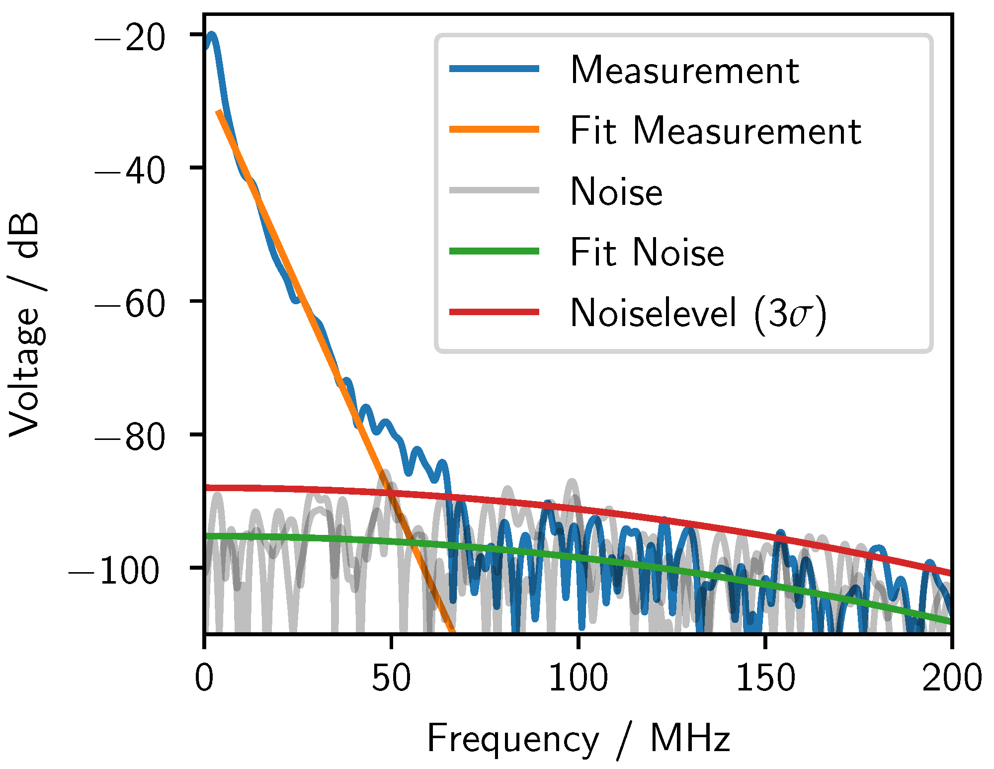
To decide up to which frequency there was still sufficient signal strength, a frequency-dependent noise level was calculated by measuring noise without any acoustic signal. The noise spectrum is Gaussian-like and is determined by the measurement setup and the digital filter used. The noise spectrum is calculated by
several times, and a quadratic formula was fitted to the averaged noise level. Three times the standard deviation of the fit residuals on top of the quadratic fit indicates the border between noise and signal (Figure 5).
The signal can be approximated by a linear decay in the logarithmic frequency spectrum [57]. Low frequencies are neglected in the linear fit due to diffraction effects (see Section 2.4.4). The intersection between the linear approximation of the signal and the approximation of the noise level defined the bandwidth of the signal. Every frequency above was interpreted as noise and was neglected.
The energy spectra shown in Section 3 are plotted as .
2.4.3. Determination of Attenuation
In addition to the phase velocity, it was also possible to calculate the frequency-resolved attenuation of the material within the path .
For the attenuation, the bandwidth was defined by the of both signals and .
Within the setup described in Section 2.1, the analysed ultrasound waves were reflected at the sample–air interface and the sample–water interface. These reflections and the associated energy transfer to the water and air had to be taken into account when calculating the attenuation. The energy remaining in the sample depends on the reflection coefficient R [58]
where the acoustic impedance . Each reflection results in an offset of the attenuation spectra and needs to be corrected. This results in the following formula
where i represents the reflections that occur between the signals and of the acoustic pulse.
2.4.4. Diffraction Correction
For small beam diameters, long propagation paths, or low frequencies, the acoustic wave can transition from the near to the far field. This transition occurs at the approximated near field length L (see Equation (10)).
A phase difference of of the acoustic wave between the near and far field distorts the determination of the phase velocity. The calculation of the attenuation in the far field is also subject to errors, as the energy decreases with distance. A correction of the phase and amplitude can be performed by calculating the diffracted wave [52]
where z is the propagation direction, is the acoustic source distribution, and i is the imaginary unit. To the best of our knowledge, there is no better correction for the approach taken.
3. Results and Discussion
With the use of simulation, we investigated the influence of the material properties of the absorption layer and the laser parameters on the excitation of the acoustic waves. These results were verified by experiments. The phase velocities of various materials were determined from further measurements.
3.1. Simulation of Material and Laser Influence on the Excitation
Simulations were carried out with the aim of characterising the influence of the material parameters of the excited object to maximise the strength of the planar compression wave. The second criterion was a high-frequency bandwidth of the acoustic pulse to maximise the frequency range from which later information can be deduced. The simulations were 2D FEM simulations (similar to Figure 4), employing both the structural mechanics and heat transfer modules from COMSOL software. (V 6.1) Both were coupled using the formula for thermal expansion.
The optical excitation was simulated by a time-dependent heat flux along the excitation line of 750 and an exponential decay of the heat flux in the depth direction with a damping factor . The thermal pulse had a constant intensity, a duration of 4 , and was completely absorbed. Different from what is usually found in the literature, we calculated the acoustic pulse in a solid absorption layer instead of a weakly absorbing fluid [59,60].
The simulations used aluminium as the material, with the parameters given in Table 1. The simulation area was larger than the penetration depth of the optical pulse.
In the simulations, the material and optical parameters were varied to determine the influence on the excited acoustic wave in the time and frequency domain. The optical parameters were laser pulse length and optical material attenuation . The laser power was kept constant as the pulse length was varied. The material parameters (thermal conductivity , coefficient of thermal expansion , specific heat capacity , density , and Young’s modulus E) were varied to cover the entire range of common materials. Appendix A contains the simulated signals and shows the dependence of these parameters on the sum of the squared elongations , which is proportional to the energy of the excited planar compression wave.
For short optical pulses, the linearly scaled frequency spectrum of the elongations can be approximated using a Gaussian function [57]. The standard deviation and the amplitude A of the Gaussian function of the autocorrelated elongations were determined. This led to the following expressions for the plane compression wave:
The formula for the squared elongations in the time domain is identical to the integral of the Gaussian function. The aim was to obtain a high elongation and a high for high-quality broadband measurements. A higher bandwidth can be achieved by a higher acoustic velocity (), stronger optical absorption, or shorter pulse durations. With the exception of the thermal expansion coefficients and the specific heat capacity, the energy cannot be optimised independently of the bandwidth. In fact, an optimisation of can simultaneously cause a worsening of . However, a smaller can often be neglected due to the higher elongations (see spectra in Appendix A).
3.2. Characterisation of Acoustic Measurement Cell
Measurements were carried out to characterise the effect of the laser pulse width, the fluid (width and type) and the excitation layer.
3.2.1. Excitation Layer
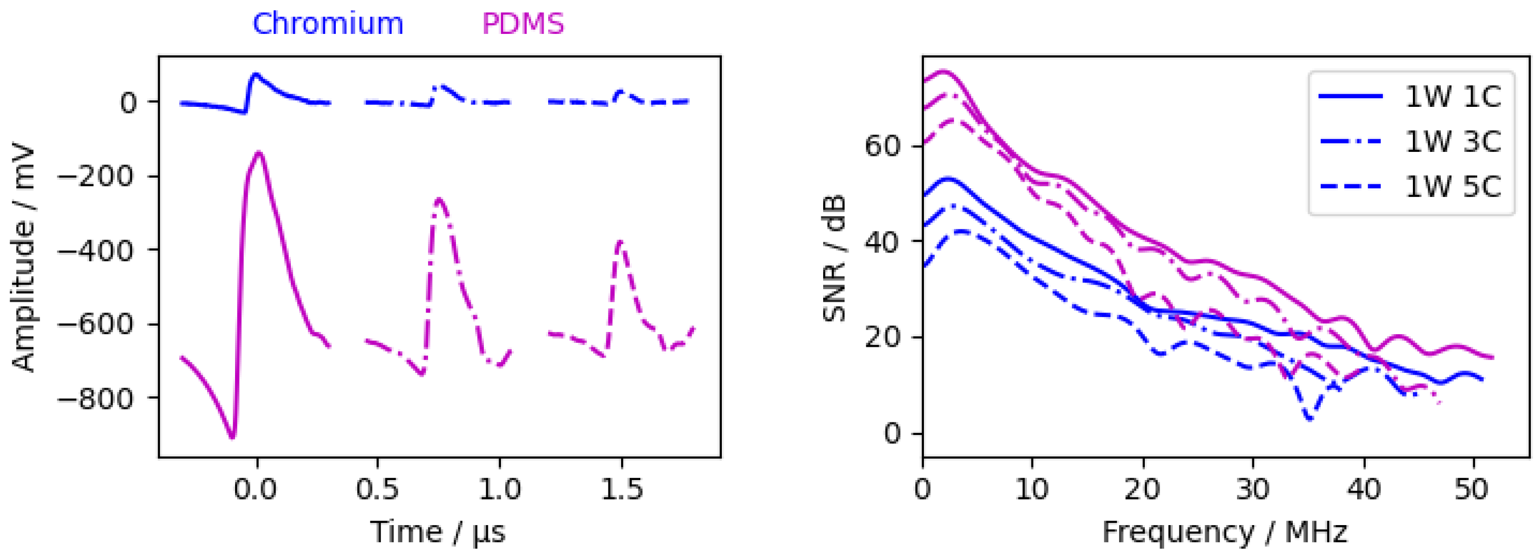
As mentioned in Section 2.3.3, measurements were carried out with two different excitation layers ( 125 chromium, 50 PDMS). The results are shown in Figure 6.
The material parameters of the PDMS layer were not known, so a comparison with Formulas (19)–(21) cannot be made. Nevertheless, it is clear that the waves excited by the PDMS layer have a higher amplitude due to the different material parameters, probably mainly due to the higher coefficient of thermal expansion and the lower specific heat capacity, Young’s modulus, and density. The amplitude of the PDMS layer is about 7 to 9 times higher than the chromium layer. As long as the SNR level is high enough, the calculated phase velocity is independent of the excitation layer.
The decrease in signal strength with higher frequencies is higher for the PDMS layer than for the chromium layer. This is predicted by the simulations and Formula (20). The lower amplitude combined with the slower decrease in signal strength resulted in a similar maximum frequency for PDMS and chromium. The waviness in the PDMS spectrum is caused by an additional wave within the signal peak. The additional wave can be seen clearer at the second peak in the time domain. This wave is even more visible in the measurement with a 1 pulsed laser (Figure 7, red circle). The reason for this additional wave is the thicker PMDS layer in which the wave is reflected.
Normally, a superposition of two waves is not desired for the phase spectrum analysis. It is, therefore, preferable to use the chromium layer as long as the amplitudes are sufficiently high.
3.2.2. Laser Pulse Width
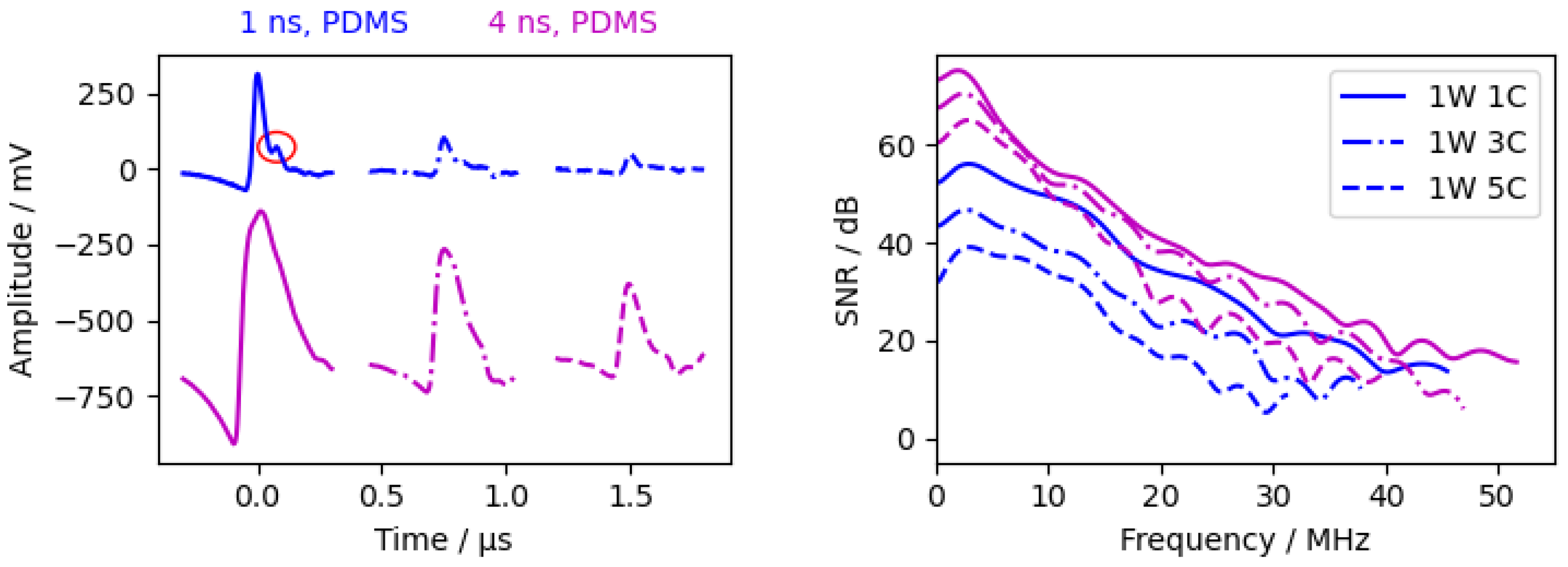
In addition to the 4 pulse laser, we performed measurements with a 1 pulse laser ( 1 pulse energy). Due to the lower pulse energy, the beam diameter had to be reduced to 2 to observe an acoustic wave (the 4 laser had a beam diameter of 18 ). The measurements are shown in Figure 7. For better visibility, the measurement signal from the 1 laser is amplified by a factor of 3.
Due to the shorter 1 pulse, the additional reflection within the PDMS layer was clearly visible in the 1W1C signal in the time domain (Figure 7, red circle). The time delay between the two peaks is , corresponding to a PDMS layer thickness of 42 . The subsequent waves decay rapidly and are barely observed. The decay between the different waves is greatly enhanced due to the small beam diameter and, therefore, the high diffraction of the acoustic pulse. The lower amplitude and slower decay in the frequency domain are analogous to the simulations (see Figure A6). The frequency spectrum of the 1W1C wave had a similar bandwidth between the different pulse lasers. This suggests that the acoustic bandwidth can be further increased by using a higher pulse energy and a 1 pulsed laser.
This suggests that the bandwidth could be further increased with a 1 laser pulse if the laser has a higher pulse energy.
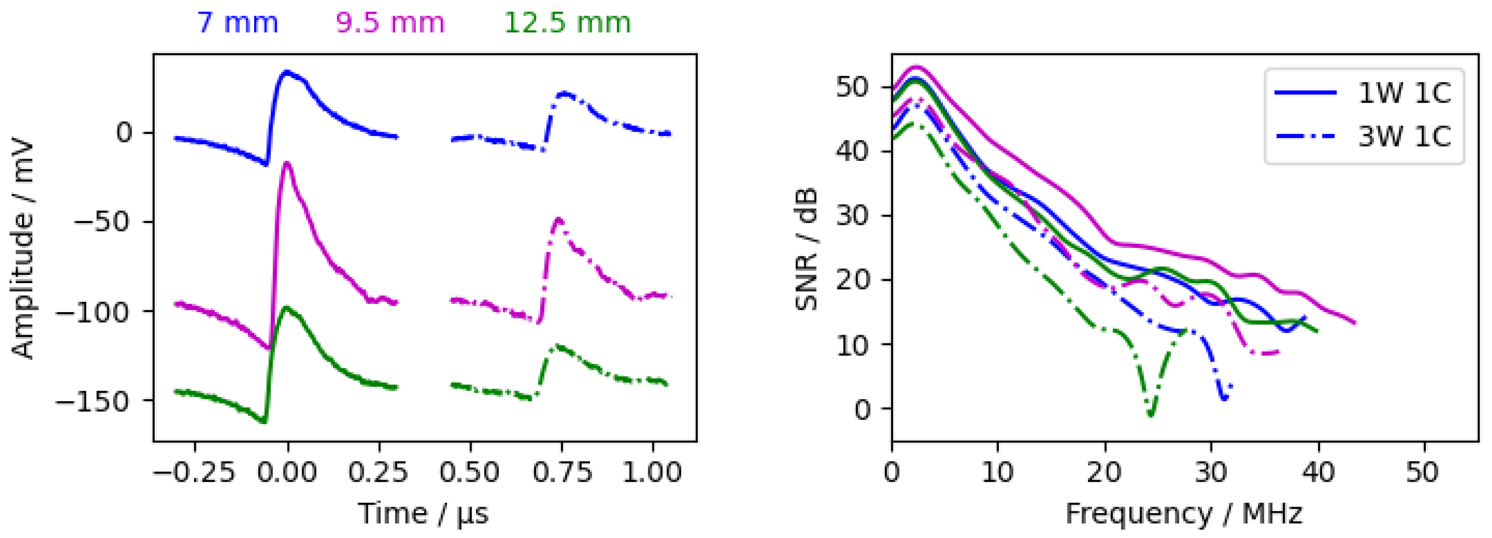
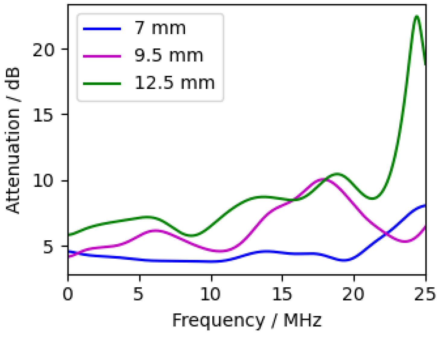
3.2.3. Water Layer Thickness
Figure 8 shows three measurements with different water layer thicknesses (with chromium as the excitation layer). The measurements showed an unexpected behaviour, as the amplitudes are significantly higher with a water layer than with a 7 water layer, although the attenuation in the measurement should be higher. In the calculated attenuation spectrum (Figure 9), the attenuation between 1W1C and 3W1C increased with increasing water thickness. Therefore, the unexpected behaviour is probably due to different levels of excitation due to laser power fluctuations. In summary, the water layer should be as thin as possible but thick enough to clearly separate the waves within the sample and the waves within the water.
3.2.4. Type of Fluid
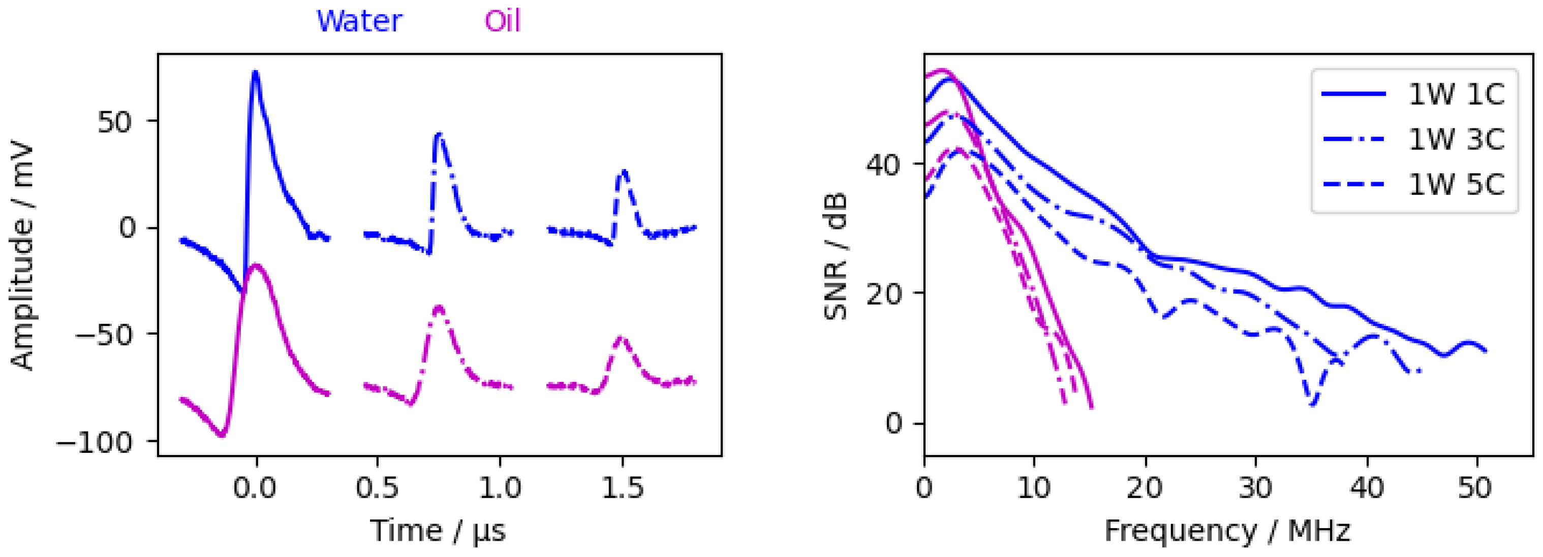
The last variable investigated was the fluid between the excitation layer and the sample. The water was replaced by a mineral hydraulic oil (HLP 46, viscosity 46 ), and the results are shown in Figure 10. The oil significantly attenuated higher frequencies, whereas lower frequencies ( ) were amplified by up to 3 dB. This suggests that oil may be a better choice for low-frequency measurements but is not suitable for frequencies above 5 . This is consistent with the literature, in which it has been reported that water typically has an attenuation of [37,39,40] and mineral oil has an attenuation of 24 [61].
3.3. Frequency Resolved Measurements in Different Materials
In this section, we show that frequency-resolved phase velocity measurements were possible in virtually any material. For this reason, we have chosen a high-velocity material (silicon single crystal), a metal (aluminium), a soft low-velocity material (silicone), and a liquid (water).
3.3.1. Silicon
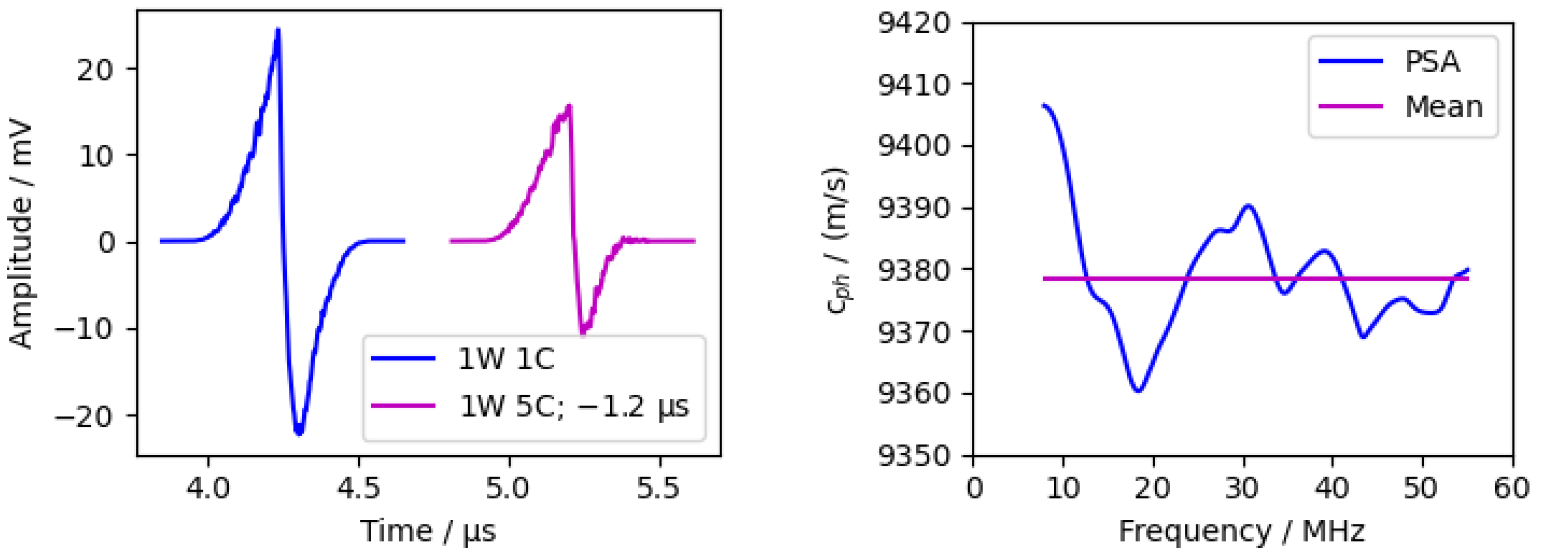
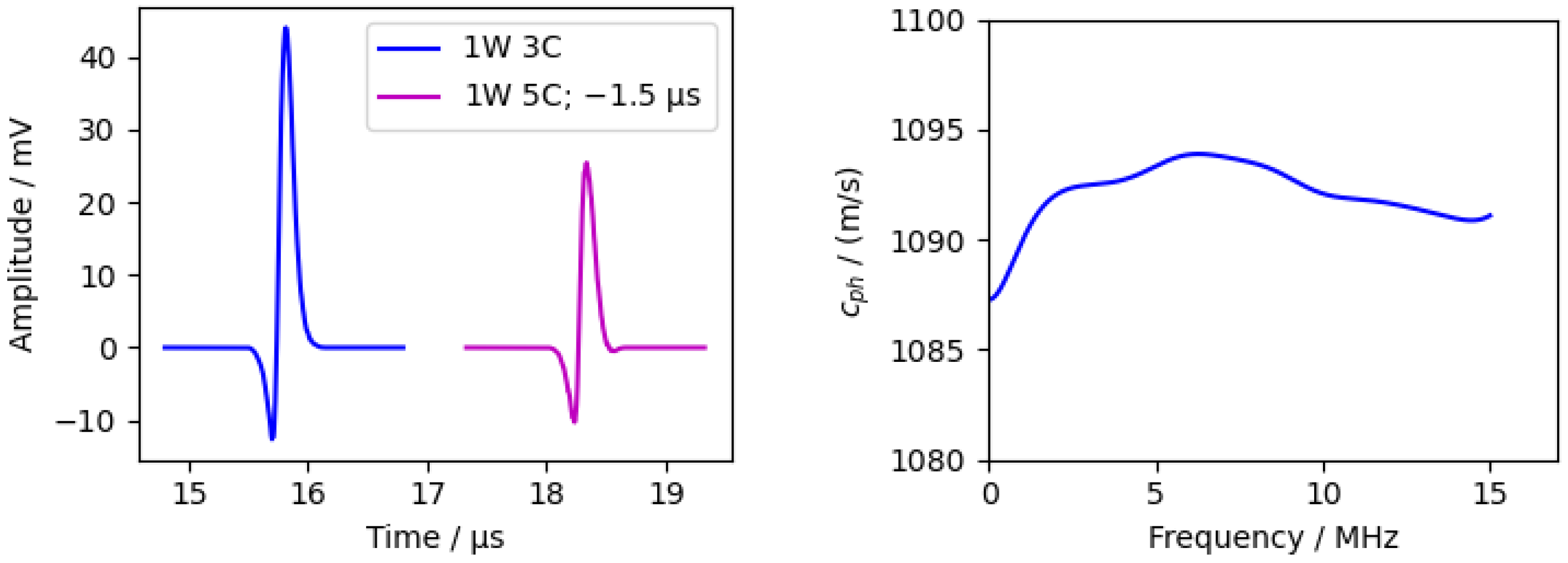
The sample used was a silicon window with a diameter and a 5 thickness. The acoustic pulse travelled along the 5 axis, which corresponds with the [111]-orientation of the silicon crystal. The measurement is visualised in Figure 11. The PDMS absorption layer was used.
The calculated phase velocity was approximated constant over the frequency with a mean value of and a standard deviation of .
3.3.2. Aluminium
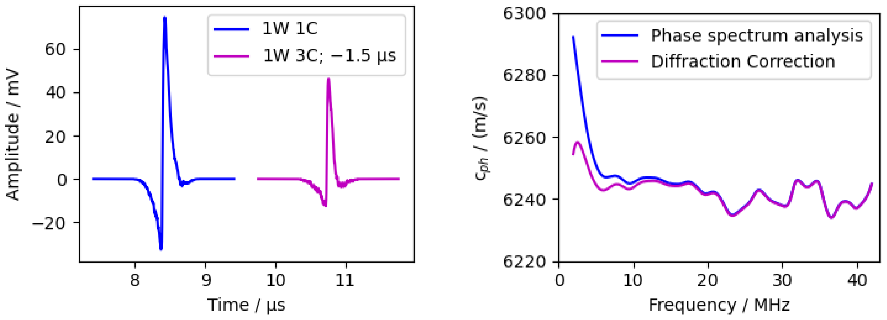
The aluminium sample was 12 thick in the measurement direction and wide enough to suppress any reflections from the sample boundaries. The absorption layer used was chromium. The results are shown in Figure 12.
The phase velocity showed a constant value for frequencies above 9 MHz with an increasing velocity towards lower frequencies. This was due to the transition between the near and far field and the resulting phase change of . The diffraction correction (Section 2.4.4) significantly reduces the increase at low frequencies and, thus, improves the result. No comparison was made between the measured sound speed and the literature data, as the literature data differ greatly due to the different alloys used (from 6200 to 6400 [35]).
3.3.3. Silicone
The silicone sample was thick and translucent. The silicone used was SF00 from “Silikonfabrik”. The absorption layer used was PDMS.
As can be seen in Figure 13, measurements in the soft silicone layer were possible up to a frequency of 15 . The measurement was made more challenging by the fact that the acoustic impedance of water and silicone is very similar; therefore, only a small proportion of the sound pulse was reflected at the interface (R~2%). This resulted in a low SNR and a low maximum frequency. With a velocity of ~1090, the measurements agree quite well with other measurements of similar materials in the literature [64,65,66].
3.3.4. Water
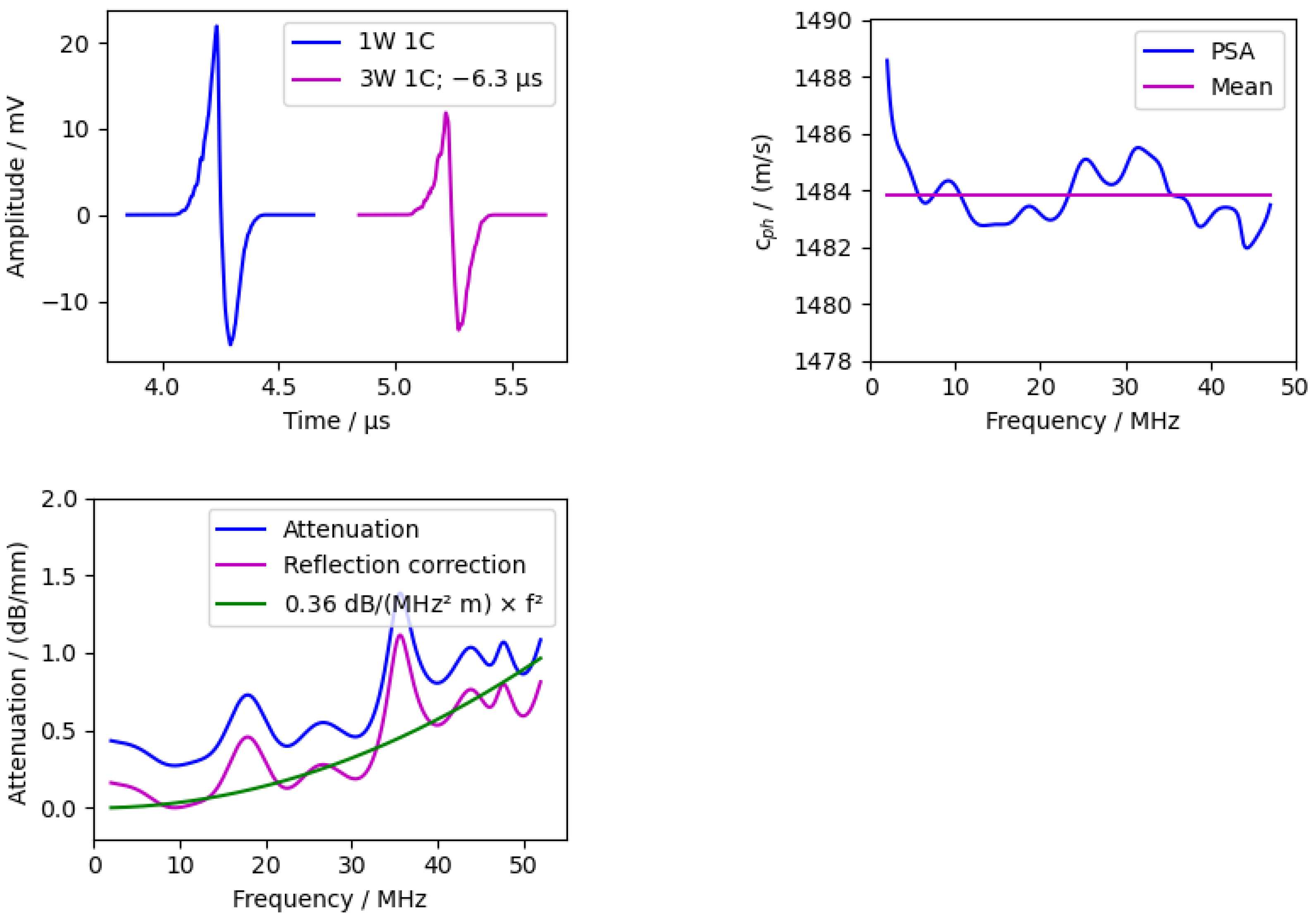
In addition, the fluid between the excitation layer and the sample can be analysed. The measurement of the silicon sample was used for this, and the reflections in the water were analysed. The results are shown in the following figures (Figure 14).
The mean velocity was with a standard deviation of 1 . The literature value for water at 20 is [67]. Considering the accuracy of the thickness measurement and the temperature uncertainty, the measurement is in good agreement.
In contrast to the previous measurements, the attenuation is also shown, as there are literature values for water with which our measuring cell can be compared. The “Reflection correction” takes into account the reflection coefficients (see Section 2.4.3). As mentioned in Section 2.3.2, the attenuation in water is usually described by a quadratic dependence on the frequency. The attenuation coefficients vary in a wide range between [37,39,40,41] and 1 [43,44] and up to 44 [36].
The measurement presented here had an attenuation coefficient of , which is between the lower and slightly higher literature values.
4. Conclusions
In this work, we presented a method to measure the longitudinal phase velocity and attenuation contactless over a high-frequency range (~3 to 55 , depending on material). We have investigated all components of the acoustic measuring cell and identified their influencing factors on the measurement. Simulations were used to analyse the excitation of compression waves. An unfocused beam with a large beam diameter is required to excite the intended planar compression waves. For the excitation of pulses with high energies, an absorption layer with a low elastic modulus, low density, low specific heat capacity, and high thermal expansion should be chosen. However, these material parameters also cause the energy of the excited acoustic waves to decrease more sharply at higher frequencies (Section 3.1). We were able to show this behaviour in a simulation and an experiment.
Therefore, polymers with additives to increase optical absorption would be suitable to excite high-energy waves. The greater decrease in energy at higher frequencies for polymers is partially offset by the increased energy. However, the experiments have shown that polymers need to be applied as a thin layer while still having a high optical absorption to suppress additional reflections of the acoustic pulse at the polymer–water and polymer–glass interfaces. These additional pulses interfere with the determination of the phase velocity and attenuation. The thin sputtered chromium layer ( 125 ) did not show the additional pulse, but the amplitude decreased by a factor of 7 to 9 in comparison with the PDMS layer. Future experiments should, therefore, consider a new polymer (-like) material for the absorption layer, which can be applied thinly and has a high optical absorption.
The water layer fulfilled the intended purpose: transmitting only the compression wave, enabling the excitation of broadband acoustic pulses independent of the sample material, and separating the waves in the time domain. The interferometer with a photorefractive crystal also showed that it can measure the acoustic pulse independent of the sample material up to high frequencies, even with weakly reflective samples.
The accuracy of the setup was demonstrated by measuring silicon and water, the sound velocities of which have been extensively analysed in the literature. The relative error was below 0.2%. The accuracy of the attenuation measurement cannot be estimated since there are no good reference materials with consistent attenuation values found in the literature. Nevertheless, the attenuation measurement for water is between the attenuation values specified in the literature.
In summary, we have developed a measurement technique that can measure the frequency-resolved phase velocity and attenuation of a sample contactlessly (only in contact with water), non-destructively, independently of the sample, and over a wide frequency range.
Author Contributions
Conceptualization, F.B.; methodology, F.B.; software, F.B.; validation, F.B.; writing—original draft preparation, F.B.; writing—review and editing, F.B. and K.S.D.; visualization, F.B.; supervision, K.S.D.; project administration, K.S.D.; funding acquisition, K.S.D. All authors have read and agreed to the published version of the manuscript.
Funding
This research was funded by the funding program “Photonics Research Germany” of the German Federal Ministry of Education and Research (grant number: 13N15899).
Institutional Review Board Statement
Not applicable.
Informed Consent Statement
Not applicable.
Data Availability Statement
The data presented in this study are available on request from the corresponding author.
Acknowledgments
The authors would like to thank Sandra Ebert for making the absorption layers.
Conflicts of Interest
The authors declare no conflicts of interest.
Appendix A. Simulation of Laser-Based Excitation of Ultrasonic Waves
This appendix details the simulations in Section 3.1 to characterise the influence of the absorption layer.
Simulations were performed in which different material and laser properties were varied in order to observe the effect on the amplitude and the frequency spectrum of the excited acoustic compression pulse. The material parameters were selected to cover the entire range of common materials.
The time signals of the elongation on the symmetry axis in a depth of is plotted. The elongations of the time signals are scaled to the elongation of the original material properties (see Table 1). The frequency spectra of the pulses are equally normalised to the original material parameters.
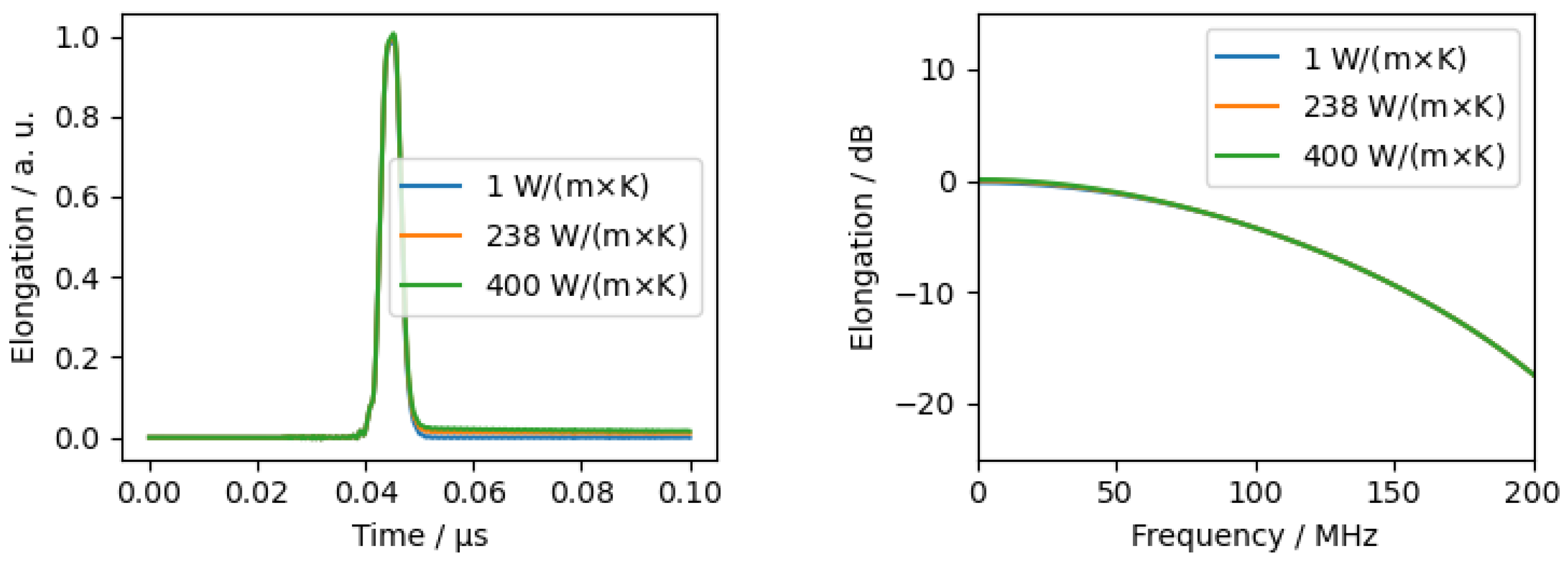
The influence of the thermal material properties (thermal conductivity, coefficient of thermal expansion, and specific heat capacity) can be seen in Figure A1, Figure A2 and Figure A3. The thermal conductivity has no influence on the elongation nor the frequency spectrum. This is due to the fact, that the heat diffusion is rather slow compared to the penetration depth, the duration of the time of the heat pulse and the acoustic wave propagation. This results in an almost stable temperature profile.
Figure A1.
FEM-Simulation with different thermal conductivity.

Figure A2.
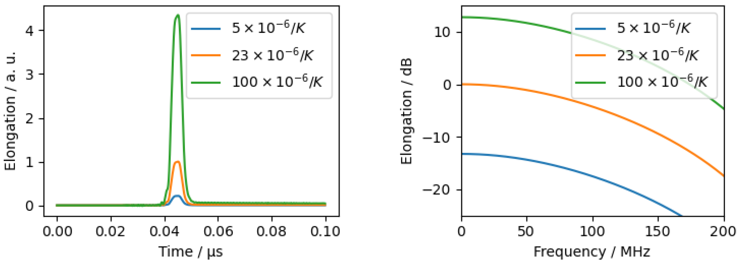
FEM-Simulation with different coefficient of thermal expansion.

Figure A3.
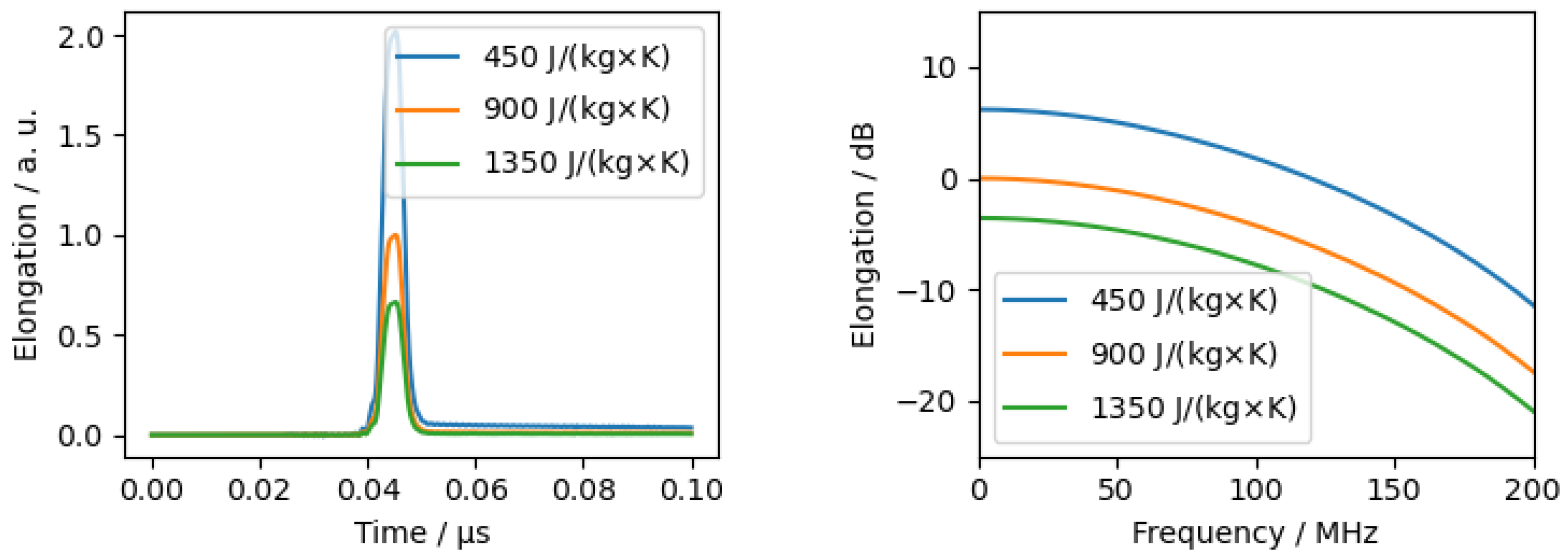
FEM-Simulation with a different specific heat capacity.

The thermal expansion and the specific heat capacity had a strong effect on the excited elongation . Both were quite intuitive, as the amplitude of the acoustic pulse depends on the temperature increase during thermal excitation and the associated thermal expansion. As the pulse shape does not change, the frequency spectrum is the same with the exception of an offset.
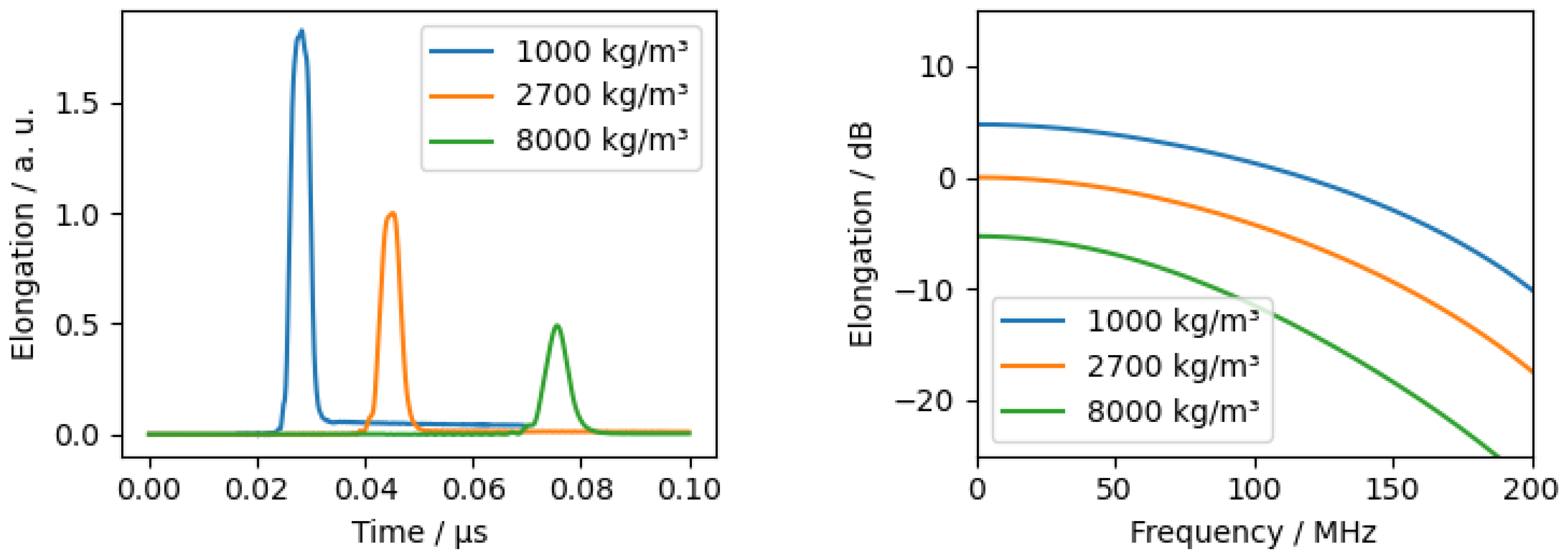
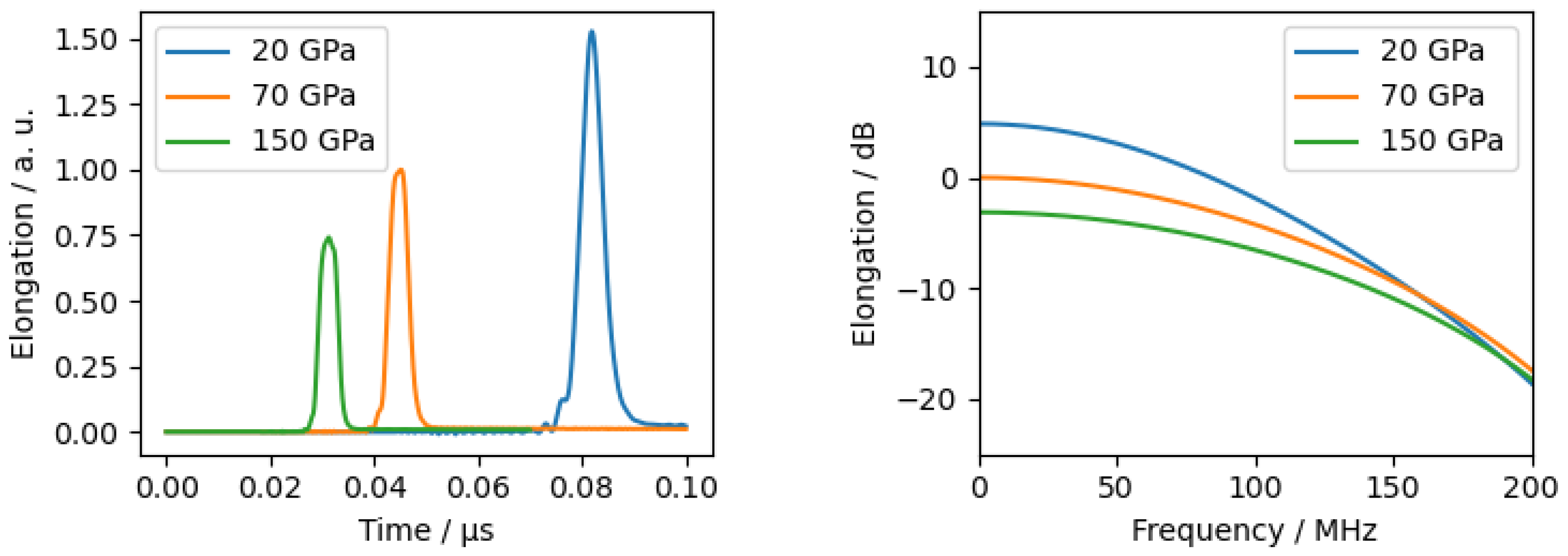
The mechanical properties (density and Young’s modulus) affected the speed of sound in the material. It can be seen that the mechanical parameters influenced the converted sound amplitude and the frequency spectra in both the time and frequency domain.
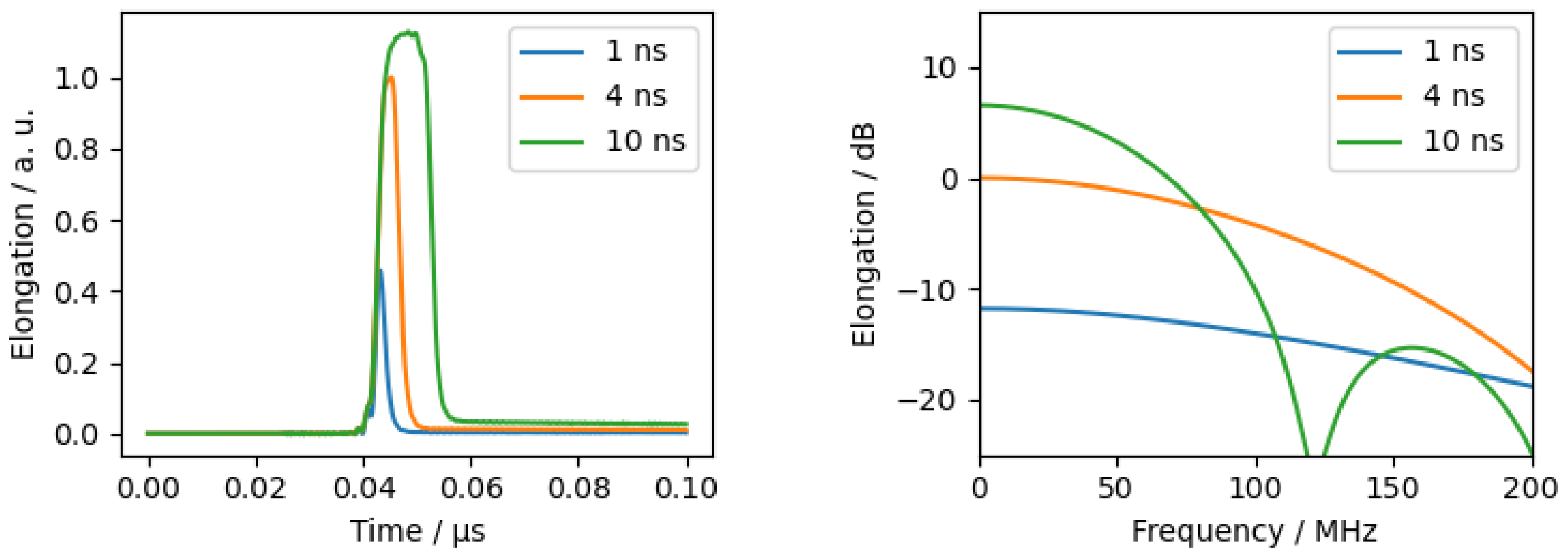
The excitation parameters (laser, respectively, heat pulse duration and the optical absorption coefficient) are shown in Figure A6 and Figure A7. The pulse duration had a significant effect on the frequency bandwidth as well as the elongation. It should be noted that when varying the pulse duration, the introduced thermal power was kept constant in the simulation and therefore the pulse energy increases at longer pulse durations.
For the variation of the attenuation of the optical material, the inserted thermal power was kept constant for all absorption coefficients.
Figure A4.
FEM-Simulation with different densities.

Figure A5.
FEM-Simulation with different Young’s moduli.

Figure A6.
FEM-Simulation with different heat pulse length.

Figure A7.
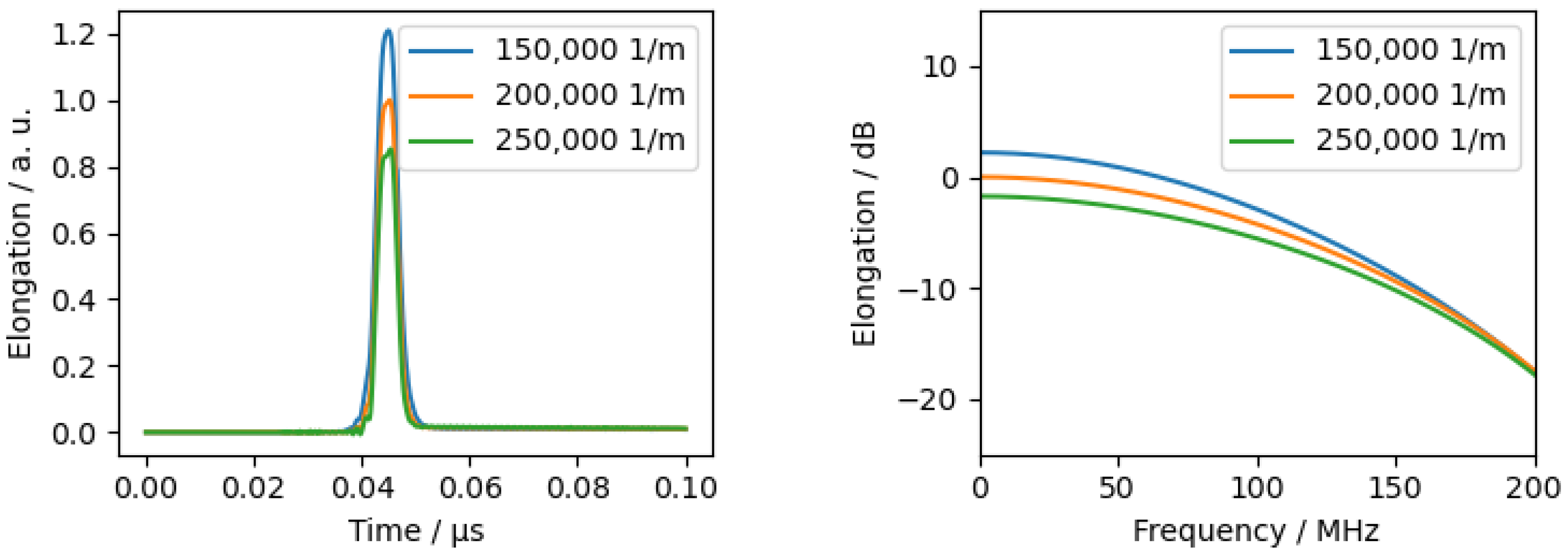
FEM-Simulation with different material absorption coefficient.

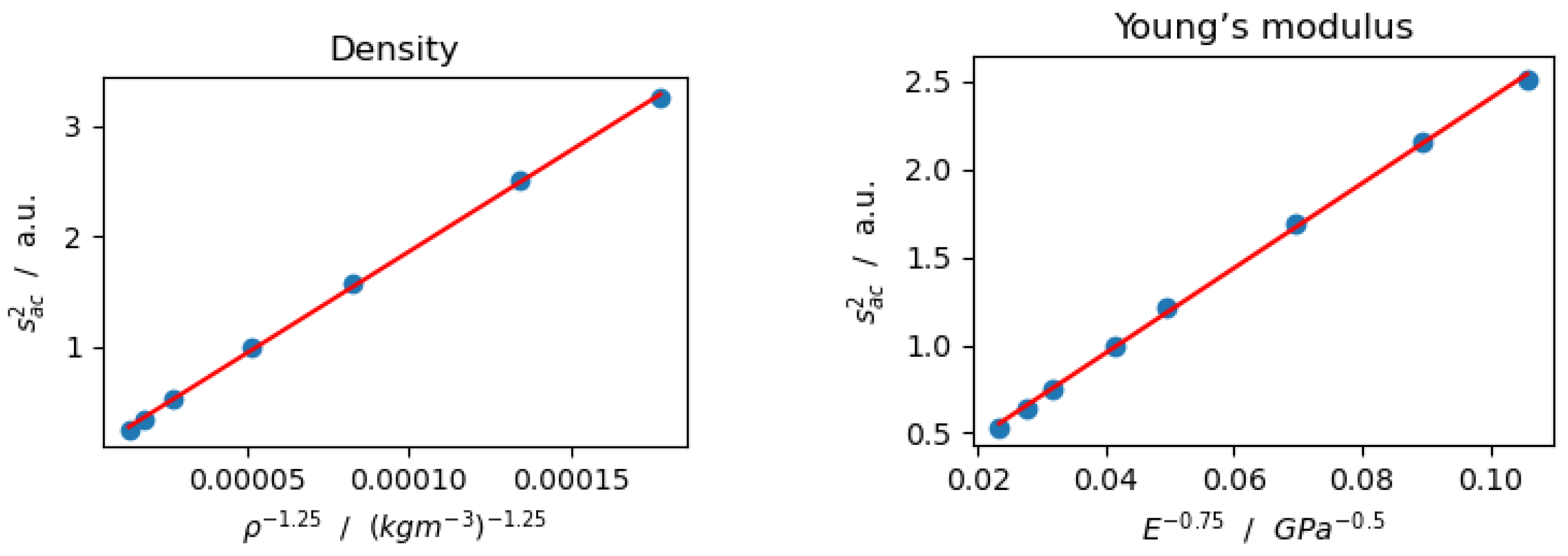
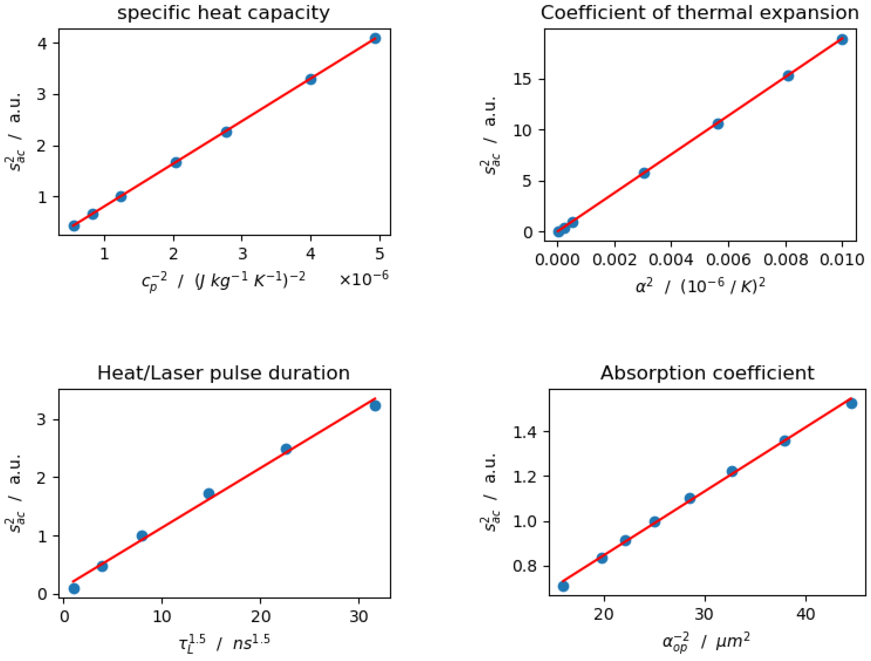
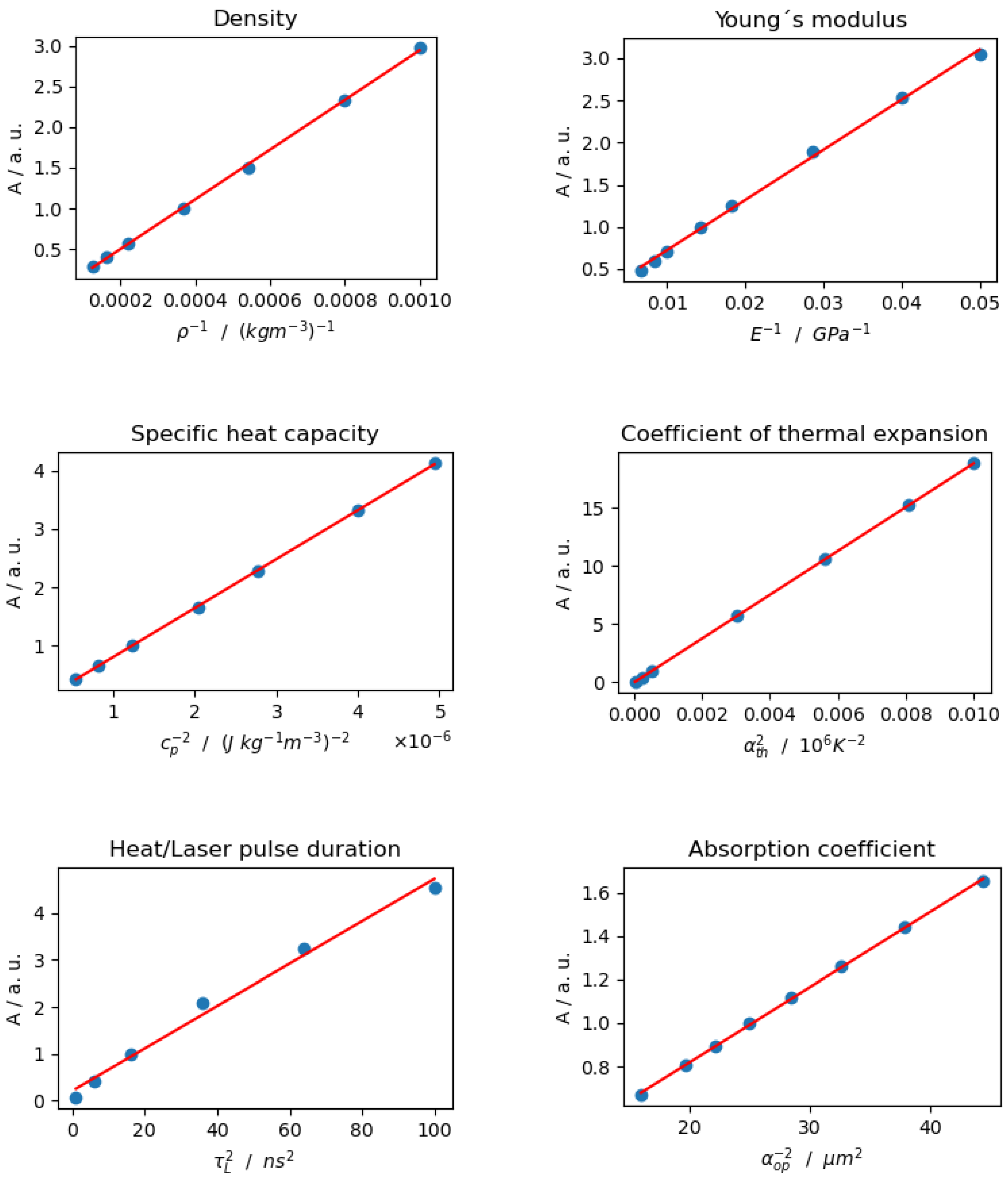
On the basis of the time signals and spectra shown in Figure A1, Figure A2, Figure A3, Figure A4, Figure A5, Figure A6 and Figure A7 it was possible to derive various dependencies between the sum of the squared elongation , the standard deviation and the amplitude A of the Gaussian fit in the linear scaled spectrum. The dependencies are visualised in the following figures and summarised in Formulas (19)–(21) in Section 3.1.
Figure A8.
Dependencies of material and excitation parameters on the elongation .


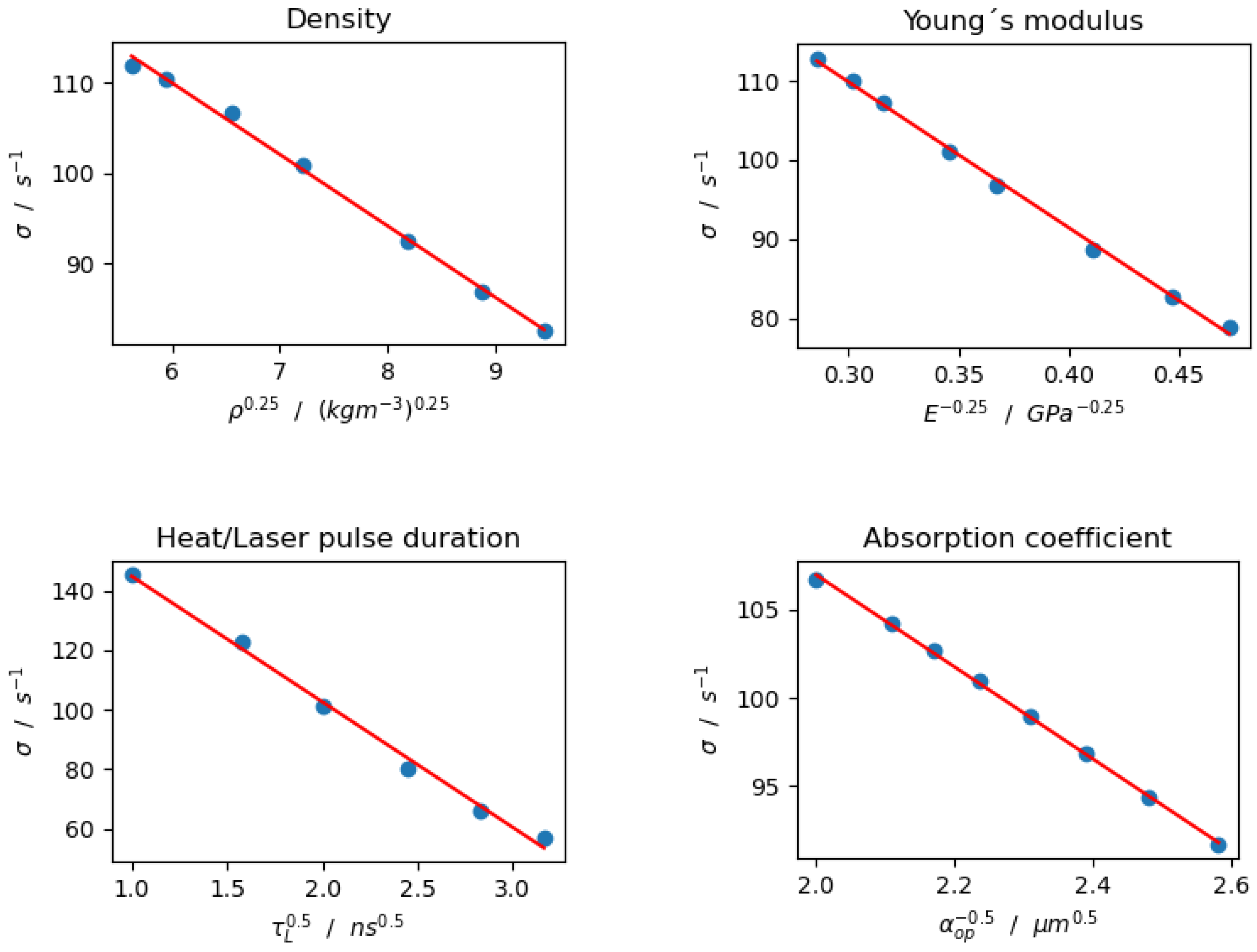
Figure A9.
Dependencies of the material and excitation parameters on the parameter.

Figure A10.
Dependencies of material and excitation parameters on the A parameter.

References
- Sharpe, W.N. (Ed.) Springer Handbook of Experimental Solid Mechanics: With 50 Tables; Springer Handbooks; Springer: New York, NY, USA, 2008. [Google Scholar]
- Barbosa, R.C.S.; Mendes, P.M. A Comprehensive Review on Photoacoustic-Based Devices for Biomedical Applications. Sensors 2022, 22, 9541. [Google Scholar] [CrossRef] [PubMed]
- Isaiev, M.; Mussabek, G.; Lishchuk, P.; Dubyk, K.; Zhylkybayeva, N.; Yar-Mukhamedova, G.; Lacroix, D.; Lysenko, V. Application of the Photoacoustic Approach in the Characterization of Nanostructured Materials. Nanomaterials 2022, 12, 708. [Google Scholar] [CrossRef] [PubMed]
- Wissmeyer, G.; Pleitez, M.A.; Rosenthal, A.; Ntziachristos, V. Looking at sound: Optoacoustics with all-optical ultrasound detection. Light Sci. Appl. 2018, 7, 53. [Google Scholar] [CrossRef] [PubMed]
- Karabutov, A.A.; Podymova, N.B. Influence of the porosity on the dispersion of the phase velocity of longitudinal acoustic waves in isotropic metal matrix composites. Acoust. Phys. 2017, 63, 288–296. [Google Scholar] [CrossRef]
- Podymova, N.B.; Karabutov, A.A. Combined effects of reinforcement fraction and porosity on ultrasonic velocity in SiC particulate aluminum alloy matrix composites. Compos. Part B Eng. 2017, 113, 138–143. [Google Scholar] [CrossRef]
- Bakaric, M.; Miloro, P.; Javaherian, A.; Cox, B.T.; Treeby, B.E.; Brown, M.D. Measurement of the ultrasound attenuation and dispersion in 3D-printed photopolymer materials from 1 to 3.5 MHz. J. Acoust. Soc. Am. 2021, 150, 2798–2805. [Google Scholar] [CrossRef]
- Jacquet, J.R.; Levassort, F.; Ossant, F.; Gregoire, J.M. 3D printed phantom for high frequency ultrasound imaging. In Proceedings of the IEEE International Ultrasonics Symposium (IUS), Taipei, Taiwan, 21–24 October 2015; pp. 1–4. [Google Scholar]
- Demčenko, A.; Akkerman, R.; Nagy, P.B.; Loendersloot, R. Non-collinear wave mixing for non-linear ultrasonic detection of physical ageing in PVC. NDT E Int. 2012, 49, 34–39. [Google Scholar] [CrossRef]
- Goldsberry, B.M.; Haberman, M.R. Negative stiffness honeycombs as tunable elastic metamaterials. J. Appl. Phys. 2018, 123, 091711. [Google Scholar] [CrossRef]
- Wang, J.; Allein, F.; Boechler, N.; Friend, J.; Vazquez-Mena, O. Design and Fabrication of Negative-Refractive-Index Metamaterial Unit Cells for Near-Megahertz Enhanced Acoustic Transmission in Biomedical Ultrasound Applications. Phys. Rev. Appl. 2021, 15, 024025. [Google Scholar] [CrossRef]
- Li, Z.; Yang, D.Q.; Liu, S.L.; Yu, S.Y.; Lu, M.H.; Zhu, J.; Zhang, S.T.; Zhu, M.W.; Guo, X.S.; Wu, H.D.; et al. Broadband gradient impedance matching using an acoustic metamaterial for ultrasonic transducers. Sci. Rep. 2017, 7, 42863. [Google Scholar] [CrossRef]
- Scruby, C.B.; Drain, L.E. Laser Ultrasonics: Techniques and Applications; Hilger: Bristol, UK, 1990. [Google Scholar]
- Gusev, V.E.; Karabutov, A.A. Laser Optoacoustics; American Institute of Physics: College Park, MD, USA, 1993. [Google Scholar]
- Monchalin, J.P. Laser-Ultrasonics: Principles Furthermore, Industrial Applications. E-J. Nondestruct. Test. 2020, 25, 1–43. [Google Scholar]
- Scherleitner, E.; Reitinger, B.; Hettich, M.; Berer, T.; Burgholzer, P. Laser Ultrasonics; Springer eBook Collection; Springer: Cham, Switzerland, 2019. [Google Scholar]
- Treeby, B.E.; Cox, B.T.; Zhang, E.Z.; Patch, S.K.; Beard, P.C. Measurement of broadband temperature-dependent ultrasonic attenuation and dispersion using photoacoustics. IEEE Trans. Ultrason. Ferroelectr. Freq. Control 2009, 56, 1666–1676. [Google Scholar] [CrossRef]
- Bai, X.; Ma, J.; Xu, W.; Wang, J.; Liu, S. Off-epicentral measurement of laser-ultrasonic shear-wave velocity and its application to elastic-moduli evaluation. Ultrasonics 2023, 127, 106850. [Google Scholar] [CrossRef]
- Messaoudi, M.; Pouet, B. Recent development in all-optical ultrasonic shear wave inspection. Nondestruct. Test. Diagn. 2018, 3, 31–34. [Google Scholar]
- Yi, D.; Pei, C.; Liu, T.; Chen, Z. Inspection of cracks with focused angle beam laser ultrasonic wave. Appl. Acoust. 2019, 145, 1–6. [Google Scholar] [CrossRef]
- Singer, F. Laser-Ultrasonic Measurement of Elastic Properties of Anodized Aluminum Coatings. Phys. Procedia 2015, 70, 334–337. [Google Scholar] [CrossRef]
- Singer, F.; Kufner, M. Model based laser-ultrasound determination of hardness gradients of gas-carburized steel. NDT E Int. 2017, 88, 24–32. [Google Scholar] [CrossRef]
- Singer, F.; Kufner, M.; Drese, K. The Influence of Excitation and Detection Methods in Laser-Ultrasonics on Precise Material Characterization. In Proceedings of the Sensoren und Messsysteme—19. ITG/GMA-Fachtagung, Nürnberg, Germany, 26–27 June 2018. [Google Scholar]
- Schneider, D. Laser-Induced Surface Acoustic Waves for Material Testing; Springer eBook Collection; Springer: Cham, Switzerland, 2019. [Google Scholar]
- Veres, I.A.; Berer, T.; Burgholzer, P. Numerical modeling of thermoelastic generation of ultrasound by laser irradiation in the coupled thermoelasticity. Ultrasonics 2013, 53, 141–149. [Google Scholar] [CrossRef]
- Dewhurst, R.J.; Edwards, C.; McKie, A.D.W.; Palmer, S.B. Estimation of the thickness of thin metal sheet using laser generated ultrasound. Appl. Phys. Lett. 1987, 51, 1066–1068. [Google Scholar] [CrossRef]
- Burrows, S.E.; Dutton, B.; Dixon, S. Laser generation of Lamb waves for defect detection: Experimental methods and finite element modeling. IEEE Trans. Ultrason. Ferroelectr. Freq. Control 2012, 59, 82–89. [Google Scholar] [CrossRef]
- Hosoya, N.; Umino, R.; Kanda, A.; Kajiwara, I.; Yoshinaga, A. Lamb wave generation using nanosecond laser ablation to detect damage. J. Vib. Control 2018, 24, 5842–5853. [Google Scholar] [CrossRef]
- Gao, W.; Glorieux, C.; Thoen, J. Laser ultrasonic study of Lamb waves: Determination of the thickness and velocities of a thin plate. Int. J. Eng. Sci. 2003, 41, 219–228. [Google Scholar] [CrossRef]
- Kamshilin, A.A.; Romashko, R.V.; Kulchin, Y.N. Adaptive interferometry with photorefractive crystals. J. Appl. Phys. 2009, 105, 031101. [Google Scholar] [CrossRef]
- Blouin, A.; Monchalin, J.P. Detection of ultrasonic motion of a scattering surface by two-wave mixing in a photorefractive GaAs crystal. Appl. Phys. Lett. 1994, 65, 932. [Google Scholar] [CrossRef]
- Campagne, B.; Blouin, A.; Pujol, L.; Monchalin, J.P. Compact and fast response ultrasonic detection device based on two-wave mixing in a gallium arsenide photorefractive crystal. Rev. Sci. Instrum. 2001, 72, 2478–2482. [Google Scholar] [CrossRef]
- Dewhurst, R.J.; Shan, Q. Optical remote measurement of ultrasound. Meas. Sci. Technol. 1999, 10, R139–R168. [Google Scholar] [CrossRef]
- Monchalin, J.P. Laser-Ultrasonics: From the Laboratory to Industry. AIP Conf. Proc. 2004, 700, 3–31. [Google Scholar]
- Ono, K. A Comprehensive Report on Ultrasonic Attenuation of Engineering Materials, Including Metals, Ceramics, Polymers, Fiber-Reinforced Composites, Wood, and Rocks. Appl. Sci. 2020, 10, 2230. [Google Scholar] [CrossRef]
- Martinez, R.; Leija, L.; Vera, A. Ultrasonic attenuation in pure water: Comparison between through-transmission and pulse-echo techniques. In Proceedings of the 2010 Pan American Health Care Exchanges IEEE, Lima, Peru, 15–19 March 2010; pp. 81–84. [Google Scholar]
- Liu, Y.; Bond, L.J.; Hu, H. Ultrasonic-Attenuation-Based Technique for Ice Characterization Pertinent to Aircraft Icing Phenomena. AIAA J. 2017, 55, 1602–1609. [Google Scholar] [CrossRef]
- Krautkrämer, J.; Krautkrämer, H. Ultrasonic Testing of Materials, 4th ed.; Springer: Berlin/Heidelberg, Germany, 1990. [Google Scholar]
- Zell, K.; Sperl, J.I.; Vogel, M.W.; Niessner, R.; Haisch, C. Acoustical properties of selected tissue phantom materials for ultrasound imaging. Phys. Med. Biol. 2007, 52, N475–N484. [Google Scholar] [CrossRef]
- Lai, T.Y.; Bruce, M.; Averkiou, M.A. Modeling of the Acoustic Field Produced by Diagnostic Ultrasound Arrays in Plane and Diverging Wave Modes. IEEE Trans. Ultrason. Ferroelectr. Freq. Control 2019, 66, 1158–1169. [Google Scholar] [CrossRef]
- Laugier, P.; Haïat, G. Bone Quantitative Ultrasound; Springer: Dordrecht, The Netherlands, 2011. [Google Scholar]
- Ye, S.G.; Harasiewicz, K.A.; Pavlin, C.J.; Foster, F.S. Ultrasound characterization of normal ocular tissue in the frequency range from 50 MHz to 100 MHz. IEEE Trans. Ultrason. Ferroelectr. Freq. Control 1995, 42, 8–14. [Google Scholar] [CrossRef]
- Richardson, E.G. Ultrasonic Physics, 2nd ed.; Elsevier Science: Burlington, ON, Canada, 1962. [Google Scholar]
- Tang, X.M.; Toksöz, M.N.; Cheng, C.H. Elastic wave radiation and diffraction of a piston source. J. Acoust. Soc. Am. 1990, 87, 1894–1902. [Google Scholar] [CrossRef]
- Schlegel, W.; Karger, C.; Jäkel, O.; Bachert, P. (Eds.) Medizinische Physik: Grundlagen-Bildgebung-Therapie-Technik; Lehrbuch, Springer Spektrum: Berlin, Germany, 2018. [Google Scholar]
- Humphrey, V.F. Ultrasound and matter–physical interactions. Prog. Biophys. Mol. Biol. 2007, 93, 195–211. [Google Scholar] [CrossRef]
- Aussel, J.D.; Le Brun, A.; Baboux, J.C. Generating acoustic waves by laser: Theoretical and experimental study of the emission source. Ultrasonics 1988, 26, 245–255. [Google Scholar] [CrossRef]
- Davies, S.J.; Edwards, C.; Taylor, G.S.; Palmer, S.B. Laser-generated ultrasound: Its properties, mechanisms and multifarious applications. J. Phys. D Appl. Phys. 1993, 26, 329–348. [Google Scholar] [CrossRef]
- Hutchins, D.; Dewhurst, R.; Palmer, S. Laser generated ultrasound at modified metal surfaces. Ultrasonics 1981, 19, 103–108. [Google Scholar] [CrossRef]
- Schlengermann, U. Über die Verwendung der Begriffe Nahfeld und Fernfeld in der Ultraschall-Werkstoffprüfung. Mater. Test. 1973, 15, 161–166. [Google Scholar] [CrossRef]
- Lee, T.; Cheong, Y.; Baac, H.W.; Guo, L.J. Origin of Gouy Phase Shift Identified by Laser-Generated Focused Ultrasound. ACS Photonics 2020, 7, 3236–3245. [Google Scholar] [CrossRef]
- Singer, F.; Kufner, M.; Drese, K. Measurement of Stress in Mechanical Components with a Novel Laser-Ultrasound Measurement System. In Proceedings of the 12th European Conference on Non-Destructive Testing (ECNDT 2018), Gothenburg, Sweden, 11–15 June 2018; Volume 23. [Google Scholar]
- Schiebold, K. Ultraschallprüfsysteme. In Zerstörungsfreie Werkstoffprüfung—Ultraschallprüfung; Schiebold, K., Ed.; Springer: Berlin/Heidelberg, Germany, 2015; pp. 35–69. [Google Scholar]
- Kossoff, G. Analysis of focusing action of spherically curved transducers. Ultrasound Med. Biol. 1979, 5, 359–365. [Google Scholar] [CrossRef] [PubMed]
- Sachse, W.; Pao, Y.H. On the determination of phase and group velocities of dispersive waves in solids. J. Appl. Phys. 1978, 49, 4320–4327. [Google Scholar] [CrossRef]
- Singer, F. Mess- und Analysemethoden in der Laserakustik bei breitbandiger Laseranregung. Tm—Tech. Mess. 2015, 82, 45–51. [Google Scholar] [CrossRef]
- Lee, T.; Baac, H.W.; Li, Q.; Guo, L.J. Efficient Photoacoustic Conversion in Optical Nanomaterials and Composites. Adv. Opt. Mater. 2018, 6, 1800491. [Google Scholar] [CrossRef]
- Rose, J.L. Ultrasonic Guided Waves in Solid Media; Cambridge University Press: New York, NY, USA, 2014. [Google Scholar]
- Ostrovskaya, G.V. Efficiency of optical-to-acoustic energy conversion upon the interaction of a pulsed laser radiation with a liquid: I. Calculation of the efficiency upon acoustooptic interaction. Tech. Phys. 2002, 47, 1299–1305. [Google Scholar] [CrossRef]
- Li, Q.; Zhao, X.; Fang, S.; Liang, F.; Chen, Z. Theoretical analysis for conversion efficiency of laser generation of acoustic waves in liquid. In Proceedings of the 2016 International Conference on Numerical Simulation of Optoelectronic Devices (NUSOD), Sydney, Australia, 11–15 July 2016; pp. 169–170. [Google Scholar]
- Liang, S.; Lashkari, B.; Choi, S.S.S.; Ntziachristos, V.; Mandelis, A. The application of frequency-domain photoacoustics to temperature-dependent measurements of the Grüneisen parameter in lipids. Photoacoustics 2018, 11, 56–64. [Google Scholar] [CrossRef] [PubMed]
- Ioffe Physico-Technical Institute. Silicon: Mechanical Properties, Elastic Constants, Lattice Vibrations. Available online: https://www.ioffe.ru/SVA/NSM/Semicond/Si/mechanic.html (accessed on 17 November 2023).
- COMSOL Multiphysics. Material Library: Si-Silicon (Single-Crystal, Anisotropic); COSMOL: Stockholm, Sweden, 2023. [Google Scholar]
- Folds, D.L. Speed of sound and transmission loss in silicone rubbers at ultrasonic frequencies. J. Acoust. Soc. Am. 1974, 56, 1295–1296. [Google Scholar] [CrossRef]
- Cafarelli, A.; Miloro, P.; Verbeni, A.; Carbone, M.; Menciassi, A. Speed of sound in rubber-based materials for ultrasonic phantoms. J. Ultrasound 2016, 19, 251–256. [Google Scholar] [CrossRef] [PubMed]
- Xu, G.; Ni, Z.; Chen, X.; Tu, J.; Guo, X.; Bruus, H.; Zhang, D. Acoustic Characterization of Polydimethylsiloxane for Microscale Acoustofluidics. Phys. Rev. Appl. 2020, 13, 054069. [Google Scholar] [CrossRef]
- Lubbers, J.; Graaff, R. A simple and accurate formula for the sound velocity in water. Ultrasound Med. Biol. 1998, 24, 1065–1068. [Google Scholar] [CrossRef]
Figure 2.
Complete measurement setup. Green: excitation, red: detection; ND: neutral density filter, BE: beam expander, M: mirror, WP: waveplate, PBS: polarizing beam splitter, L: lens, BPD: balanced photodetector.
Figure 2.
Complete measurement setup. Green: excitation, red: detection; ND: neutral density filter, BE: beam expander, M: mirror, WP: waveplate, PBS: polarizing beam splitter, L: lens, BPD: balanced photodetector.

Figure 3.
Directivity of compression and shear waves for point sources in case of aluminium.

Figure 4.
Simulation of excited waves in aluminium via heat impulse after 75 . C: compression wave; S: shear wave; R: Rayleigh wave; H: head wave; PC: plane compression wave. Colour scale corresponds to particle velocity.
Figure 4.
Simulation of excited waves in aluminium via heat impulse after 75 . C: compression wave; S: shear wave; R: Rayleigh wave; H: head wave; PC: plane compression wave. Colour scale corresponds to particle velocity.

Figure 5.
Determination of noise level from numerous noise measurements (grey signals) and the quadratic fit. The intersection of the noise level and the linear fit of the measurement data defined the maximum frequency of the signal.
Figure 5.
Determination of noise level from numerous noise measurements (grey signals) and the quadratic fit. The intersection of the noise level and the linear fit of the measurement data defined the maximum frequency of the signal.

Figure 6.
Measurements with different excitation layers. (Left) time signal from interferometer. PDMS signals have an offset of . (Right) calculated SNR according Section 2.4.2.
Figure 6.
Measurements with different excitation layers. (Left) time signal from interferometer. PDMS signals have an offset of . (Right) calculated SNR according Section 2.4.2.

Figure 7.
Measurements with different excitation layers. (Left) time signal from interferometer. The 1 signal was amplified by 3, the 4 signals have an offset of , and the red circle shows the reflection within the PDMS layer. (Right) calculated SNR according Section 2.4.2.
Figure 7.
Measurements with different excitation layers. (Left) time signal from interferometer. The 1 signal was amplified by 3, the 4 signals have an offset of , and the red circle shows the reflection within the PDMS layer. (Right) calculated SNR according Section 2.4.2.

Figure 8.
Measurements with different water layer thicknesses with chromium as excitation layer. (Left) time signal from the interferometer. The measurement has an offset of , and the measurement has an offset of . (Right) calculated SNR according Section 2.4.2.
Figure 8.
Measurements with different water layer thicknesses with chromium as excitation layer. (Left) time signal from the interferometer. The measurement has an offset of , and the measurement has an offset of . (Right) calculated SNR according Section 2.4.2.

Figure 9.
Frequency-resolved attenuation of measurements with different water layer thicknesses (Equation (15)). Compared peaks are 1W1C and 3W1C. Excitation layer was chromium.
Figure 9.
Frequency-resolved attenuation of measurements with different water layer thicknesses (Equation (15)). Compared peaks are 1W1C and 3W1C. Excitation layer was chromium.

Figure 10.
Measurements with oil and water between excitation layer and specimen. Chromium was used as excitation layer. (Left) time signal from the interferometer. Oil signals have an offset of . (Right) calculated SNR according to Section 2.4.2.
Figure 10.
Measurements with oil and water between excitation layer and specimen. Chromium was used as excitation layer. (Left) time signal from the interferometer. Oil signals have an offset of . (Right) calculated SNR according to Section 2.4.2.

Figure 11.
Measurement of 5 thick silicon sample. (Left) time domain with shifted second peak. (Right) phase velocity calculated via phase spectrum analysis (PSA).
Figure 11.
Measurement of 5 thick silicon sample. (Left) time domain with shifted second peak. (Right) phase velocity calculated via phase spectrum analysis (PSA).

Figure 12.
Measurement of 12 mm thick aluminium sample. (Left) time domain with shifted second peak. (Right) phase velocity calculated via phase spectrum analysis (PSA).
Figure 12.
Measurement of 12 mm thick aluminium sample. (Left) time domain with shifted second peak. (Right) phase velocity calculated via phase spectrum analysis (PSA).

Figure 13.
Measurement of thick silicone sample. (Left) time domain with shifted second peak. (Right) phase velocity calculated via phase spectrum analysis (PSA).
Figure 13.
Measurement of thick silicone sample. (Left) time domain with shifted second peak. (Right) phase velocity calculated via phase spectrum analysis (PSA).

Figure 14.
Measurement of thick water layer between PDMS absorption layer and silicon window. (Left) time domain with shifted second peak. (Right) phase velocity calculated via phase spectrum analysis (PSA). (Bottom) attenuation of water with quadratic fit.
Figure 14.
Measurement of thick water layer between PDMS absorption layer and silicon window. (Left) time domain with shifted second peak. (Right) phase velocity calculated via phase spectrum analysis (PSA). (Bottom) attenuation of water with quadratic fit.


Table 1.
Used material properties for the FEM simulation.
| Elastic modulus E | 70 |
| Density | 2700 |
| Poisson ratio | 0.33 |
| Coefficient of thermal expansion | |
| Thermal conductivity | 238 |
| Specific heat capacity | 900 |
Disclaimer/Publisher’s Note: The statements, opinions and data contained in all publications are solely those of the individual author(s) and contributor(s) and not of MDPI and/or the editor(s). MDPI and/or the editor(s) disclaim responsibility for any injury to people or property resulting from any ideas, methods, instructions or products referred to in the content. |
© 2024 by the authors. Licensee MDPI, Basel, Switzerland. This article is an open access article distributed under the terms and conditions of the Creative Commons Attribution (CC BY) license (https://creativecommons.org/licenses/by/4.0/).
Share and Cite
MDPI and ACS Style
Brand, F.; Drese, K.S. Frequency-Resolved High-Frequency Broadband Measurement of Acoustic Longitudinal Waves by Laser-Based Excitation and Detection. Sensors 2024, 24, 1630. https://doi.org/10.3390/s24051630
AMA Style
Brand F, Drese KS. Frequency-Resolved High-Frequency Broadband Measurement of Acoustic Longitudinal Waves by Laser-Based Excitation and Detection. Sensors. 2024; 24(5):1630. https://doi.org/10.3390/s24051630
Chicago/Turabian StyleBrand, Felix, and Klaus Stefan Drese. 2024. "Frequency-Resolved High-Frequency Broadband Measurement of Acoustic Longitudinal Waves by Laser-Based Excitation and Detection" Sensors 24, no. 5: 1630. https://doi.org/10.3390/s24051630
Note that from the first issue of 2016, this journal uses article numbers instead of page numbers. See further details here.