
Linear and Non-Linear Heart Rate Variability Indexes from Heart-Induced Mechanical Signals Recorded with a Skin-Interfaced IMU †
 , ,
, ,  , , and
Abstract
:1. Introduction
2. Materials and Methods
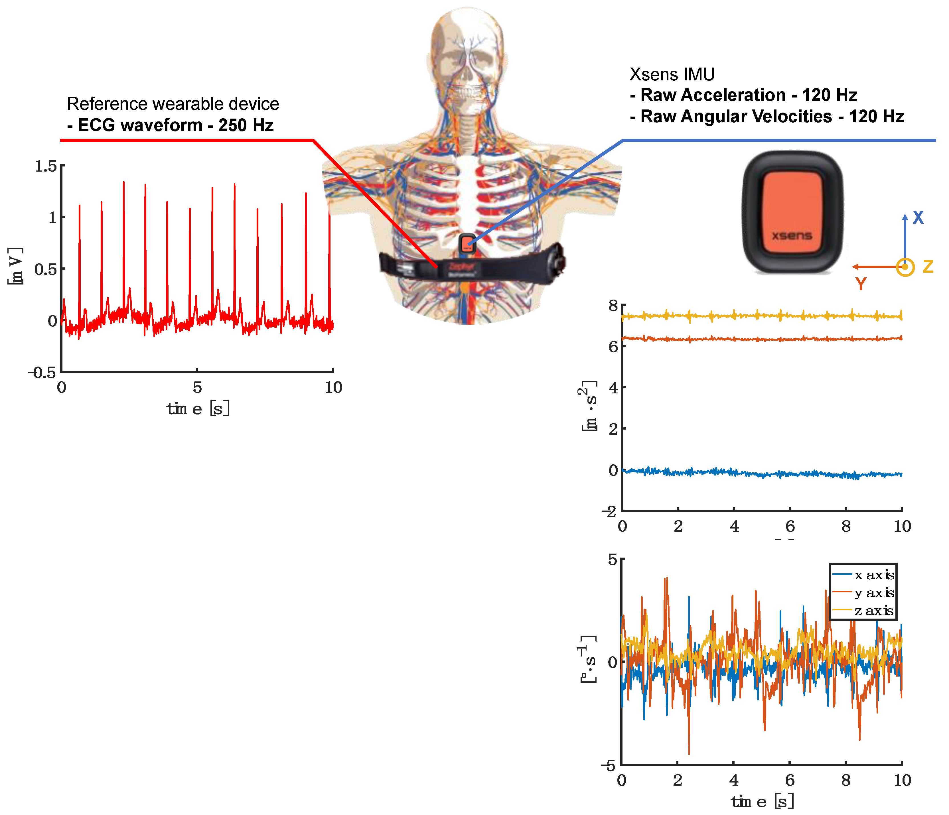
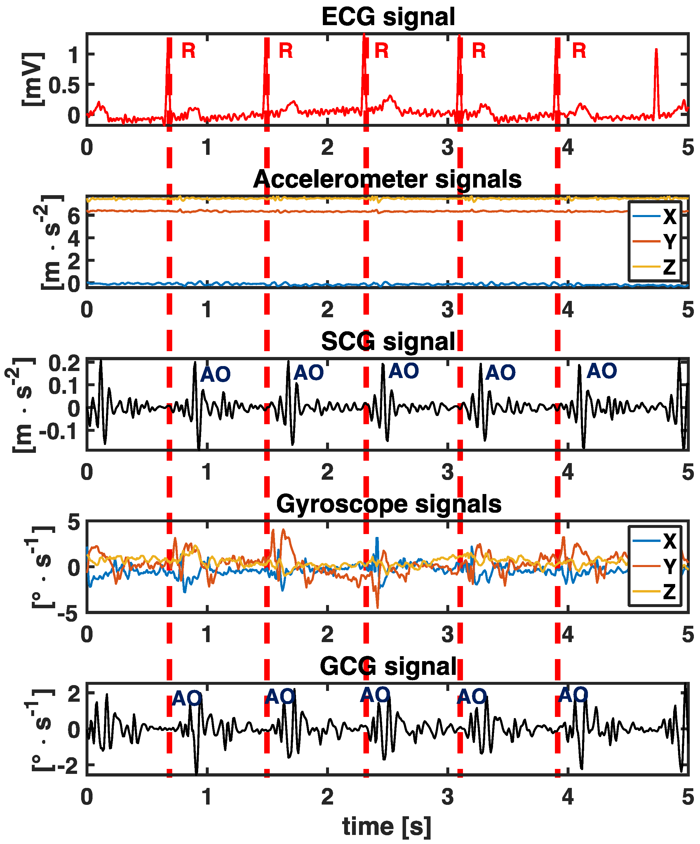
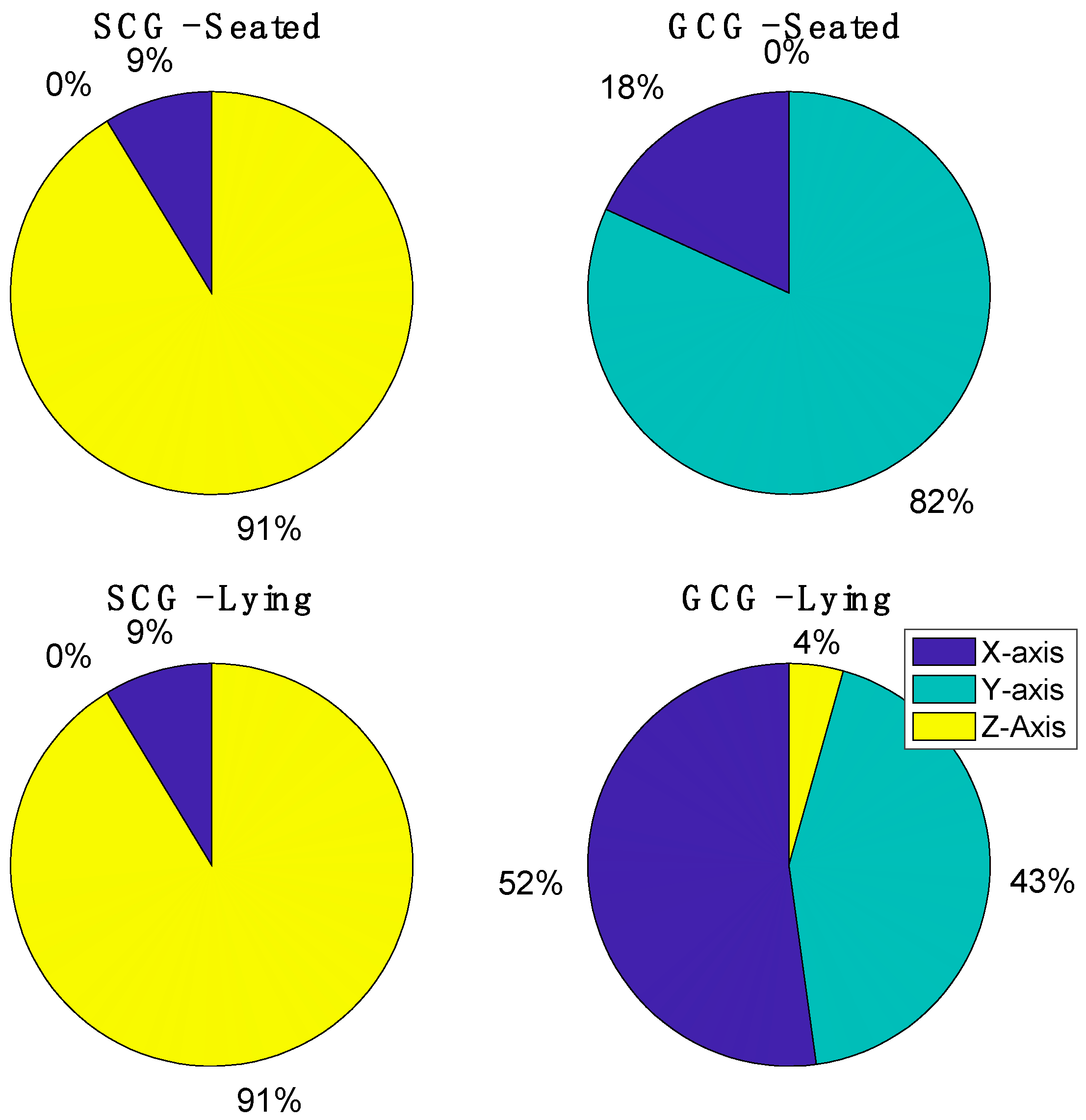
2.1. SCG and GCG Signals
2.2. ECG Signals
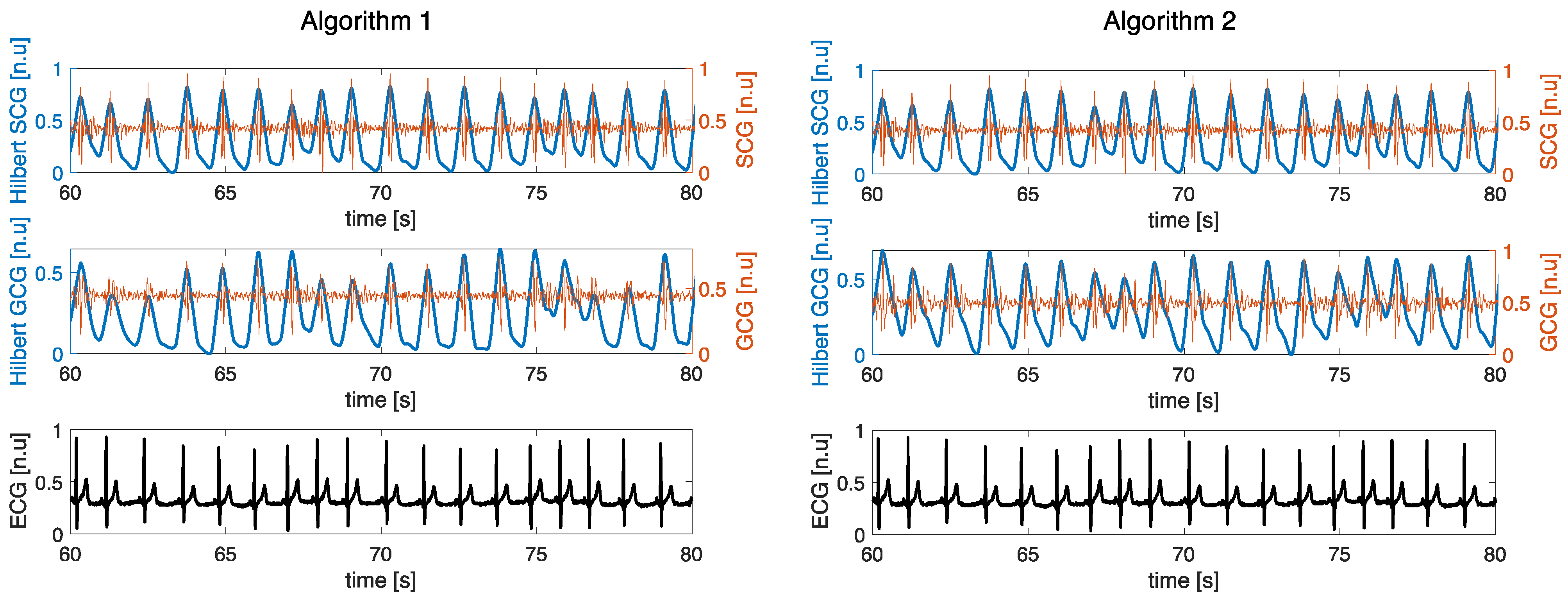
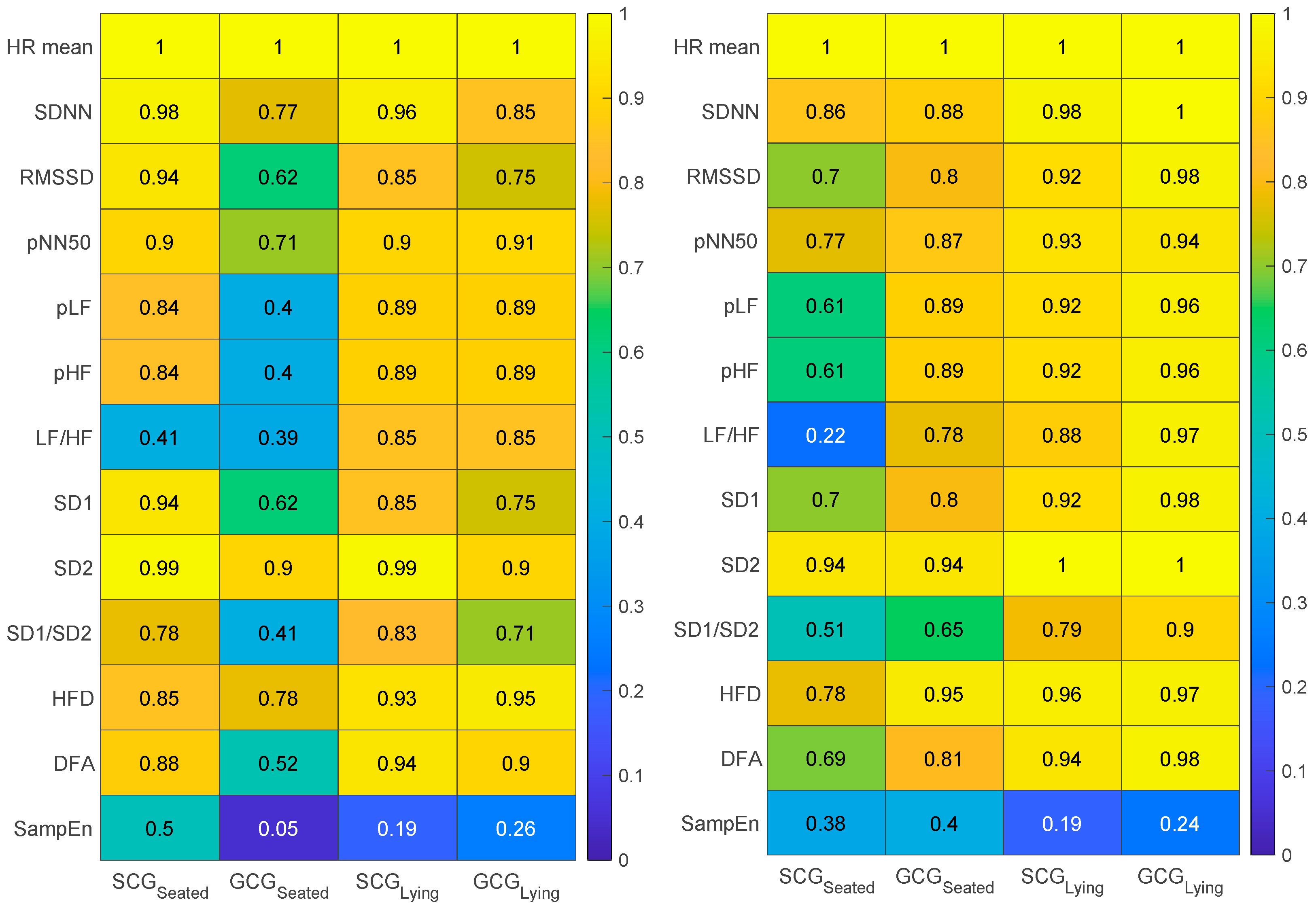
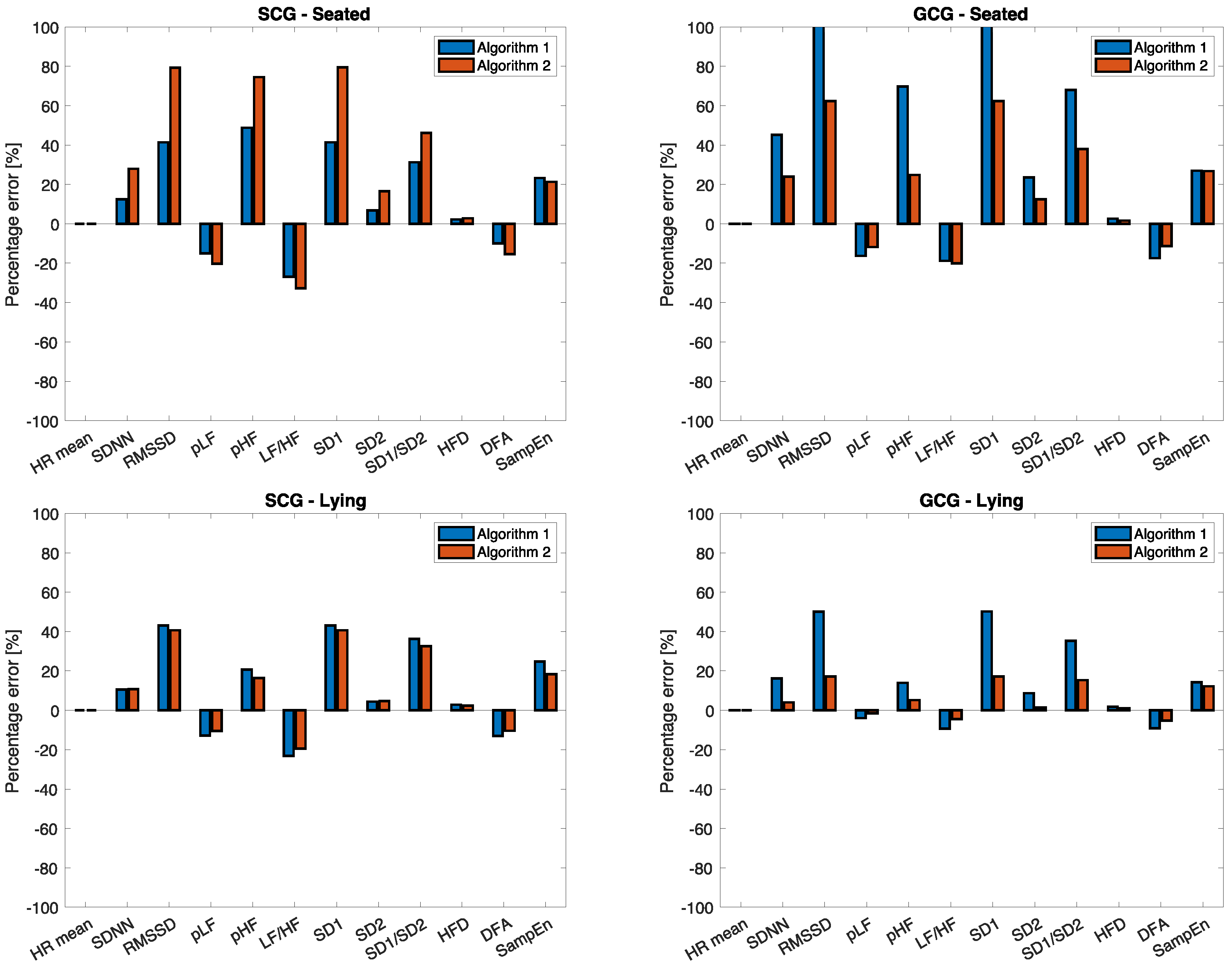
2.3. Data Analysis
- Mean heart rate (HR mean);
- Standard deviation of all IBI (SDNN);
- Root mean square of differences (RMSSD);
- The proportion for which the successive IBI differences exceed 50 milliseconds (pNN50);
- the percentage of power of the very low-frequency band (from 0.0033 Hz to 0.04 Hz, VLF);
- the percentage of power of the low-frequency band (from 0.04 Hz to 0.15 Hz, LF);
- the percentage of power of the high-frequency band (from 0.15 Hz to 0.4 Hz, HF)
- the ratio between low and high frequencies (LF/HF).
- SD1 as the standard deviation of the orthogonal distances of the / obtained in the Poincaré Plot. SD1 is considered to describe the short-term HRV;
- SD2 as the standard deviation of the orthogonal distances of the / to the length diameter of the ellipse obtained in the Poincaré Plot. SD2 is considered to describe the long-term HRV;
- Ratio between SD1 to SD2 (SD1/SD2) representing balanced ANS;
- Higuchi Fractal Dimension (HFD) measures complexity directly in time series [53];
- Detrended Fluctuation Analysis (DFA), a modified random-walk method, quantifies the fractal-like scaling properties of RR interval series [54];
- Sample entropy (SampEn), a regularity statistic that measures the irregularity (or unpredictability) of the signal [55].
3. Results
4. Discussion and Conclusions
Author Contributions
Funding
Institutional Review Board Statement
Informed Consent Statement
Data Availability Statement
Conflicts of Interest
References
- Benjamin, E.J.; Muntner, P.; Alonso, A.; Bittencourt, M.S.; Callaway, C.W.; Carson, A.P.; Chamberlain, A.M.; Chang, A.R.; Cheng, S.; Das, S.R.; et al. Heart Disease and Stroke Statistics-2019 Update: A Report From the American Heart Association. Circulation 2019, 139, e56–e528. [Google Scholar] [CrossRef]
- Nichols, M.; Townsend, N.; Scarborough, P.; Rayner, M. Cardiovascular Disease in Europe: Epidemiological Update. Eur. Heart J. 2013, 34, 3028–3034. [Google Scholar] [CrossRef]
- Franciosi, S.; Perry, F.K.G.; Roston, T.M.; Armstrong, K.R.; Claydon, V.E.; Sanatani, S. The Role of the Autonomic Nervous System in Arrhythmias and Sudden Cardiac Death. Auton. Neurosci. Basic Clin. 2017, 205, 1–11. [Google Scholar] [CrossRef]
- Barron, H.V.; Lesh, M.D. Autonomic Nervous System and Sudden Cardiac Death. J. Am. Coll. Cardiol. 1996, 27, 1053–1060. [Google Scholar] [CrossRef]
- Johnson, B.K. Physiology of the Autonomic Nervous System. In Basic Sciences in Anesthesia; Farag, E., Argalious, M., Tetzlaff, J.E., Sharma, D., Eds.; Springer International Publishing: Cham, Switzerland, 2018; pp. 355–364. ISBN 978-3-319-62067-1. [Google Scholar]
- Kors, J.A.; Swenne, C.A.; Greiser, K.H. Cardiovascular Disease, Risk Factors, and Heart Rate Variability in the General Population. J. Electrocardiol. 2007, 40, S19–S21. [Google Scholar] [CrossRef]
- Fox, K.; Borer, J.S.; Camm, A.J.; Danchin, N.; Ferrari, R.; Lopez Sendon, J.L.; Steg, P.G.; Tardif, J.C.; Tavazzi, L.; Tendera, M. Resting Heart Rate in Cardiovascular Disease. J. Am. Coll. Cardiol. 2007, 50, 823–830. [Google Scholar] [CrossRef]
- Stein, P.K.; Reddy, A. Non-Linear Heart Rate Variability and Risk Stratification in Cardiovascular Disease. Indian Pacing Electrophysiol. J. 2005, 5, 210–220. [Google Scholar]
- Thayer, J.F.; Yamamoto, S.S.; Brosschot, J.F. The Relationship of Autonomic Imbalance, Heart Rate Variability and Cardiovascular Disease Risk Factors. Int. J. Cardiol. 2010, 141, 122–131. [Google Scholar] [CrossRef]
- Hartmann, R.; Schmidt, F.M.; Sander, C.; Hegerl, U. Heart Rate Variability as Indicator of Clinical State in Depression. Front. Psychiatry 2019, 9, 735. [Google Scholar] [CrossRef]
- Sgoifo, A.; Carnevali, L.; Pico Alfonso, M.D.L.A.; Amore, M. Autonomic Dysfunction and Heart Rate Variability in Depression. Stress 2015, 18, 343–352. [Google Scholar] [CrossRef]
- Čukić, M.; Savić, D.; Sidorova, J. When Heart Beats Differently in Depression: A Review of HRV Measures. arXiv 2022, arXiv:2110.08621. [Google Scholar]
- Makivić, B.; Nikić, M.D.; Willis, M.S. Heart Rate Variability (HRV) as a Tool for Diagnostic and Monitoring Performance in Sport and Physical Activities. J. Exerc. Physiol. Online 2013, 16, 103–131. [Google Scholar]
- Shaffer, F.; Ginsberg, J.P. An Overview of Heart Rate Variability Metrics and Norms. Front. Public Health 2017, 5, 258. [Google Scholar] [CrossRef] [PubMed] [Green Version]
- Billman, G.E. Heart Rate Variability—A Historical Perspective. Front. Physiol. 2011, 2, 86. [Google Scholar] [CrossRef] [PubMed]
- De Pinho Ferreira, N.; Gehin, C.; Massot, B. A Review of Methods for Non-Invasive Heart Rate Measurement on Wrist. IRBM 2021, 42, 4–18. [Google Scholar] [CrossRef]
- Santucci, F.; Lo Presti, D.; Massaroni, C.; Schena, E.; Setola, R. Precordial Vibrations: A Review of Wearable Systems, Signal Processing Techniques, and Main Applications. Sensors 2022, 22, 5805. [Google Scholar] [CrossRef]
- Lo Presti, D.; Massaroni, C.; D’Abbraccio, J.; Massari, L.; Caponero, M.; Longo, U.G.; Formica, D.; Oddo, C.M.; Schena, E. Wearable System Based on Flexible Fbg for Respiratory and Cardiac Monitoring. IEEE Sens. J. 2019, 19, 7391–7398. [Google Scholar] [CrossRef]
- Massaroni, C.; Zaltieri, M.; Lo Presti, D.; Nicolò, A.; Tosi, D.; Schena, E. Fiber Bragg Grating Sensors for Cardiorespiratory Monitoring: A Review. IEEE Sens. J. 2021, 21, 14069–14080. [Google Scholar] [CrossRef]
- Centracchio, J.; Andreozzi, E.; Esposito, D.; Gargiulo, G.D.; Bifulco, P. Detection of Aortic Valve Opening and Estimation of Pre-Ejection Period in Forcecardiography Recordings. Bioengineering 2022, 9, 89. [Google Scholar] [CrossRef]
- Romano, C.; Schena, E.; Formica, D.; Massaroni, C. Comparison between Chest-Worn Accelerometer and Gyroscope Performance for Heart Rate and Respiratory Rate Monitoring. Biosensors 2022, 12, 834. [Google Scholar] [CrossRef]
- Taebi, A.; Solar, B.; Bomar, A.; Sandler, R.; Mansy, H. Recent Advances in Seismocardiography. Vibration 2019, 2, 64–86. [Google Scholar] [CrossRef]
- Zanetti, J.M.; Tavakolian, K. Seismocardiography: Past, Present and Future. In Proceedings of the 2013 35th Annual International Conference of the IEEE Engineering in Medicine and Biology Society (EMBC), Osaka, Japan, 3–7 July 2013; pp. 7004–7007. [Google Scholar]
- Sieciński, S.; Kostka, P.S.; Tkacz, E.J. Gyrocardiography: A Review of the Definition, History, Waveform Description, and Applications. Sensors 2020, 20, 6675. [Google Scholar] [CrossRef] [PubMed]
- Brüser, C.; Antink, C.H.; Wartzek, T.; Walter, M.; Leonhardt, S. Ambient and Unobtrusive Cardiorespiratory Monitoring Techniques. IEEE Rev. Biomed. Eng. 2015, 8, 30–43. [Google Scholar] [CrossRef]
- Siecinski, S.; Kostka, P.S.; Tkacz, E.J. Time Domain and Frequency Domain Heart Rate Variability Analysis on Gyrocardiograms. In Proceedings of the 2020 42nd Annual International Conference of the IEEE Engineering in Medicine & Biology Society (EMBC), Montreal, QC, Canada, 20–24 July 2020; pp. 2630–2633. [Google Scholar] [CrossRef]
- Garcia-Gonzalez, M.A.; Argelagos-Palau, A.; Fernandez-Chimeno, M.; Ramos-Castro, J. A Comparison of Heartbeat Detectors for the Seismocardiogram. In Proceedings of the Computing in Cardiology, Zaragoza, Spain, 22–25 September 2013; Volume 40, pp. 461–464. [Google Scholar]
- Laurin, A.; Blaber, A.; Tavakolian, K. Seismocardiograms Return Valid Heart Rate Variability Indices. Comput. Cardiol. 2013, 40, 413–416. [Google Scholar]
- Tadi, M.J.; Lahdenoja, O.; Humanen, T.; Koskinen, J.; Pankaala, M.; Koivisto, T. Automatic Identification of Signal Quality for Heart Beat Detection in Cardiac MEMS Signals. In Proceedings of the 2017 IEEE EMBS International Conference on Biomedical & Health Informatics (BHI), Orland, FL, USA, 16–19 February 2017; pp. 137–140. [Google Scholar] [CrossRef]
- Siecinski, S.; Tkacz, E.J.; Kostka, P.S. Comparison of HRV Indices Obtained from ECG and SCG Signals from CEBS Database. Biomed. Eng. Online 2019, 18, 69. [Google Scholar] [CrossRef]
- Singh, M.J.; Sharma, L.N.; Dandapat, S. Hilbert Vibration Decomposition of Seismocardiogram for HR and HRV Estimation. In Proceedings of the 2022 IEEE International Conference on Signal Processing and Communications (SPCOM), Bangalore, India, 11–15 July 2022; pp. 1–5. [Google Scholar] [CrossRef]
- Siecinski, S.; Kostka, P.S.; Tkacz, E.J. Time Domain and Frequency Domain Heart Rate Variability Analysis on Electrocardiograms and Mechanocardiograms from Patients with Valvular Diseases. In Proceedings of the 2022 44th Annual International Conference of the IEEE Engineering in Medicine & Biology Society (EMBC), Glasgow, UK, 11–15 July 2022; Volume 2022, pp. 653–656. [Google Scholar] [CrossRef]
- Sieciński, S.; Kostka, P.S.; Tkacz, E.J. Heart Rate Variability Analysis on Electrocardiograms, Seismocardiograms and Gyrocardiograms on Healthy Volunteers. Sensors 2020, 20, 4522. [Google Scholar] [CrossRef]
- Massaroni, C.; Romano, C.; De Tommasi, F.; Cukic, M.B.; Carassiti, M.; Formica, D.; Schena, E. Heart Rate and Heart Rate Variability Indexes Estimated By Mechanical Signals From A Skin-Interfaced IMU. In Proceedings of the 2022 IEEE International Workshop on Metrology for Industry 4.0 and IoT, MetroInd 4.0 and IoT 2022—Proceedings, Trento, Italy, 7–9 June 2022; pp. 322–327. [Google Scholar]
- Maiorana, E.; Massaroni, C. Biometric Recognition Based on Heart-Induced Chest Vibrations. In Proceedings of the 9th International Workshop on Biometrics and Forensics, IWBF 2021, Rome, Italy, 6–7 May 2021. [Google Scholar]
- Xsens. Xsens DOT. Available online: https://www.xsens.com/hubfs/Downloads/Manuals/Xsens%20DOT%20User%20Manual.pdf (accessed on 2 November 2022).
- Hailstone, J.; Kilding, A.E. Reliability and Validity of the ZephyrTM BioHarnessTM to Measure Respiratory Responses to Exercise. Meas. Phys. Educ. Exerc. Sci. 2011, 15, 293–300. [Google Scholar] [CrossRef]
- Rai, D.; Thakkar, H.K.; Rajput, S.S.; Santamaria, J.; Bhatt, C.; Roca, F. A Comprehensive Review on Seismocardiogram: Current Advancements on Acquisition, Annotation, and Applications. Mathematics 2021, 9, 2243. [Google Scholar] [CrossRef]
- Choudhary, T.; Sharma, L.N.; Bhuyan, M.K. Automatic Detection of Aortic Valve Opening Using Seismocardiography in Healthy Individuals. IEEE J. Biomed. Health Inform. 2019, 23, 1032–1040. [Google Scholar] [CrossRef]
- Lin, D.J.; Kimball, J.P.; Zia, J.; Ganti, V.G.; Inan, O.T. Reducing the Impact of External Vibrations on Fiducial Point Detection in Seismocardiogram Signals. IEEE Trans. Biomed. Eng. 2022, 69, 176–185. [Google Scholar] [CrossRef]
- Mora, N.; Cocconcelli, F.; Matrella, G.; Ciampolini, P. Detection and Analysis of Heartbeats in Seismocardiogram Signals. Sensors 2020, 20, 1670. [Google Scholar] [CrossRef]
- Lee, H.; Lee, H.; Whang, M. An Enhanced Method to Estimate Heart Rate from Seismocardiography via Ensemble Averaging of Body Movements at Six Degrees of Freedom. Sensors 2018, 18, 238. [Google Scholar] [CrossRef]
- Karantonis, D.M.; Narayanan, M.R.; Mathie, M.; Lovell, N.H.; Celler, B.G. Implementation of a Real-Time Human Movement Classifier Using a Triaxial Accelerometer for Ambulatory Monitoring. IEEE Trans. Inf. Technol. Biomed. 2006, 10, 156–167. [Google Scholar] [CrossRef]
- Zephyr Log Data Descriptions. 2013. Available online: https://www.zephyranywhere.com/media/download/bioharness-log-data-descriptions-07-apr-2016.pdf (accessed on 2 November 2022).
- Yang, C.; Tang, S.; Tavassolian, N. Utilizing Gyroscopes Towards the Automatic Annotation of Seismocardiograms. IEEE Sens. J. 2017, 17, 2129–2136. [Google Scholar] [CrossRef]
- Shafiq, G.; Tatinati, S.; Veluvolu, K.C. Automatic Annotation of Peaks in Seismocardiogram for Systolic Time Intervals. In Proceedings of the Annual International Conference of the IEEE Engineering in Medicine and Biology Society, EMBS 2016, Orlando, FL, USA, 16–20 August 2016; Volume 2016, pp. 2672–2675. [Google Scholar]
- Etemadi, M.; Inan, O.T. Wearable Ballistocardiogram and Seismocardiogram Systems for Health and Performance. J. Appl. Physiol. 2018, 124, 452–461. [Google Scholar] [CrossRef]
- Han, X.; Wu, X.; Wang, J.; Li, H.; Cao, K.; Cao, H.; Zhong, K.; Yang, X. The Latest Progress and Development Trend in the Research of Ballistocardiography (BCG) and Seismocardiogram (SCG) in the Field of Health Care. Appl. Sci. 2021, 11, 8896. [Google Scholar] [CrossRef]
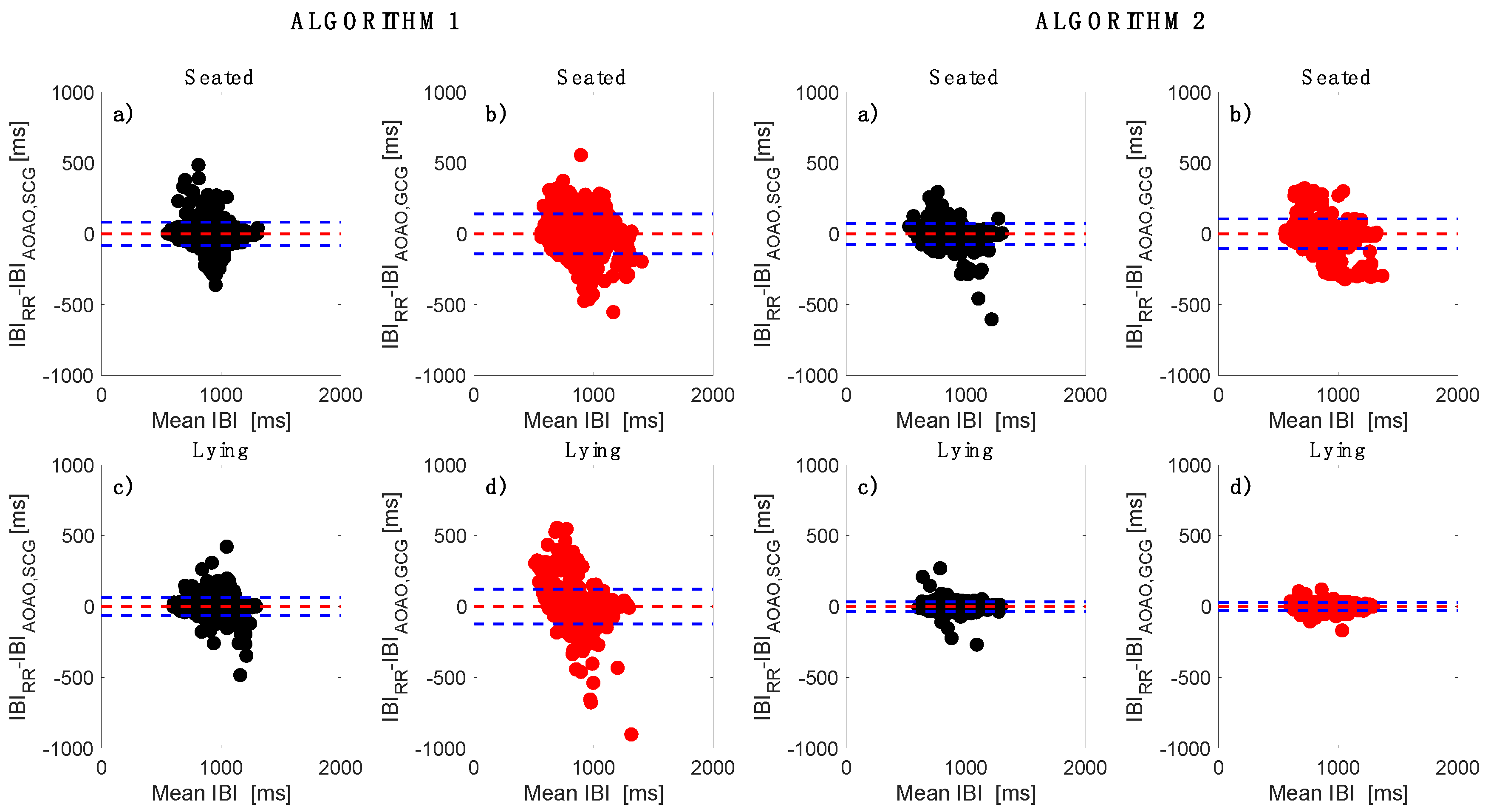
- Altman, D.G.; Bland, J.M. Measurement in Medicine: The Analysis of Method Comparison Studies. J. R. Stat. Soc. Ser. D 1983, 32, 307–317. [Google Scholar] [CrossRef]
- Giavarina, D. Understanding Bland Altman Analysis. Biochem. Medica 2015, 25, 141–151. [Google Scholar] [CrossRef]
- Abu-Arafeh, A.; Jordan, H.; Drummond, G. Reporting of Method Comparison Studies: A Review of Advice, an Assessment of Current Practice, and Specific Suggestions for Future Reports. Br. J. Anaesth. 2016, 117, 569–575. [Google Scholar] [CrossRef]
- Gerke, O. Reporting Standards for a Bland-Altman Agreement Analysis: A Review of Methodological Reviews. Diagnostics 2020, 10, 334. [Google Scholar] [CrossRef]
- Higuchi, T. Approach to an Irregular Time Series on the Basis of the Fractal Theory. Phys. D Nonlinear Phenom. 1988, 31, 277–283. [Google Scholar] [CrossRef]
- Peng, C.K.; Hausdorff, J.; Goldberger, A. Fractal Mechanisms in Neural Control: Human Heartbeat and Gait Dynamics in Health and Disease. In Self-Organized Biological Dynamics and Nonlinear Control; Cambridge University Press: Cambridge, UK, 1999. [Google Scholar]
- Richman, J.S.; Moorman, J.R. Physiological Time-Series Analysis Using Approximate Entropy and Sample Entropy. Am. J. Physiol. Heart Circ. Physiol. 2000, 278, H2039–H2049. [Google Scholar] [CrossRef] [PubMed]
- Vollmer, M. HRVTool—An Open-Source Matlab Toolbox for Analyzing Heart Rate Variability. In Proceedings of the 2019 Computing in Cardiology (CinC), Singapore, 8–11 September 2019. [Google Scholar] [CrossRef]
- Vollmer, M. A Robust, Simple and Reliable Measure of Heart Rate Variability Using Relative RR Intervals. Comput. Cardiol. 2015, 42, 609–612. [Google Scholar] [CrossRef]
- Tadi, M.J.; Lehtonen, E.; Koivisto, T.; Pankaala, M.; Paasio, A.; Teras, M. Seismocardiography: Toward Heart Rate Variability (HRV) Estimation. In Proceedings of the 2015 IEEE International Symposium on Medical Measurements and Applications, MeMeA 2015, Torino, Italy, 7–9 May 2015; pp. 261–266. [Google Scholar]
- Smits, F.M.; Porcaro, C.; Cottone, C.; Cancelli, A.; Rossini, P.M.; Tecchio, F. Electroencephalographic Fractal Dimension in Healthy Ageing and Alzheimer’s Disease. PLoS ONE 2016, 11, e0149587. [Google Scholar] [CrossRef]
- Aysin, B.; Aysin, E. Effect of Respiration in Heart Rate Variability (HRV) Analysis. In Proceedings of the 2006 International Conference of the IEEE Engineering in Medicine and Biology Society, New York, NY, USA, 30 August–3 September 2006; pp. 1776–1779. [Google Scholar] [CrossRef]
- Gasior, J.S.; Sacha, J.; Jelen, P.J.; Zielinski, J.; Przybylski, J. Heart Rate and Respiratory Rate Influence on Heart Rate Variability Repeatability: Effects of the Correction for the Prevailing Heart Rate. Front. Physiol. 2016, 7, 356. [Google Scholar] [CrossRef] [Green Version]


| Algorithm 1 | Algorithm 2 | |||||||
|---|---|---|---|---|---|---|---|---|
| Seated | Lying | Seated | Lying | |||||
| SCG | GCG | SCG | GCG | SCG | GCG | SCG | GCG | |
| R | 0.95 | 0.88 | 0.97 | 0.90 | 0.96 | 0.93 | 0.99 | 0.99 |
| MOD ± LOAs [ms] | 0.17 ± 81.66 | −1.32 ± 140.48 | −0.14 ± 63.68 | 0.59 ± 122.73 | −0.47 ± 75.41 | −0.18 ± 105.34 | −0.15 ± 33.71 | −0.13 ± 26.43 |
| Number of beats detected | 2464 | 2464 | 2274 | 2274 | 2464 | 2464 | 2274 | 2274 |
| HRV Index | Alg. | Seated | Lying | ||||
|---|---|---|---|---|---|---|---|
| ECG | SCG | GCG | ECG | SCG | GCG | ||
| HR mean [bpm] | 1 | 71.33 ± 9.93 | 71.34 ± 9.91 | 71.20 ± 9.73 | 68.29 ± 9.11 | 68.28 ± 9.11 | 68.33 ± 9.11 |
| 2 | 71.30 ± 9.96 | 71.32 ± 9.93 | 68.29 ± 9.10 | 68.29 ± 9.10 | |||
| SDNN [ms] | 1 | 67.32 ± 33.66 | 74.77 ± 36.87 | 92.06 ± 52.25 | 65.50 ± 32.42 | 69.67 ± 30.28 | 76.52 ± 47.09 |
| 2 | 80.28 ± 35.44 | 81.21 ± 50.85 | 71.02 ± 35.64 | 66.75 ± 31.77 | |||
| RMSSD [ms] | 1 | 55.00 ± 35.26 | 71.99 ± 43.01 | 104.48 ± 81.46 * | 52.85 ± 34.5 | 65.31 ± 32.53 | 76.20 ± 62.46 |
| 2 | 81.44 ± 46.21 | 84.31 ± 72.18 | 69.73 ± 45.47 | 58.40 ± 34.7 | |||
| pNN50 [%] | 1 | 30.06 ± 22.76 | 41.77 ± 25.33 | 47.83 ± 29.69 | 26.87 ± 23.36 | 34.68 ± 22.56 | 35.49 ± 25.80 |
| 2 | 46.40 ± 24.14 | 40.64 ± 23.77 | 36.77 ± 25.09 | 32.36 ± 22.94 | |||
| pLF [%] | 1 | 56.27 ± 20.80 | 47.50 ± 18.28 | 44.51 ± 22.59 | 55.59 ± 18.91 | 49.60 ± 19.71 | 51.26 ± 17.73 |
| 2 | 43.19 ± 17.85 | 50.42 ± 22.43 | 48.36 ± 19.16 | 54.12 ± 17.89 | |||
| pHF [%] | 1 | 43.72 ± 20.80 | 52.50 ± 18.28 | 55.482 ± 22.59 | 44.40 ± 18.91 | 50.39 ± 19.71 | 48.73 ± 17.73 |
| 2 | 56.80 ± 17.85 | 49.57 ± 22.43 | 51.63 ± 19.16 | 45.87 ± 17.89 | |||
| LF/HF | 1 | 2.26 ± 2.78 | 1.13 ± 0.76 | 1.16 ± 1.01 | 1.69 ±1.19 | 1.31 ± 0.95 | 1.40 ± 1.11 |
| 2 | 0.96 ± 0.73 * | 1.47 ± 1.23 | 1.24 ± 0.92 | 1.54 ± 1.05 | |||
| HRV Index | Alg. | Seated | Lying | ||||
|---|---|---|---|---|---|---|---|
| ECG | SCG | GCG | ECG | SCG | GCG | ||
| SD1 [s] | 1 | 0.04 ± 0.02 | 0.05 ± 0.03 | 0.07 ± 0.06 * | 0.04 ± 0.02 | 0.04 ± 0.02 | 0.05 ± 0.04 |
| 2 | 0.05 ± 0.03 | 0.05 ± 0.05 | 0.04 ± 0.03 | 0.04 ± 0.02 | |||
| SD2 [s] | 1 | 0.09 ± 0.04 | 0.09 ± 0.04 | 0.10 ± 0.05 | 0.08 ± 0.04 | 0.08 ± 0.04 | 0.09 ± 0.05 |
| 2 | 0.09 ± 0.04 | 0.09 ± 0.05 | 0.08 ± 0.04 | 0.08 ± 0.04 | |||
| SD1/SD2 | 1 | 0.43 ± 0.13 | 0.54 ± 0.16 | 0.68 ± 0.37 * | 0.43 ± 0.17 | 0.55 ± 0.24 | 0.56 ± 0.24 |
| 2 | 0.59 ± 0.24 | 0.58 ± 0.26 | 0.56 ± 0.23 | 0.49 ± 0.21 | |||
| HFD | 1 | 1.87 ± 0.09 | 1.90 ± 0.09 | 1.91 ± 0.09 | 1.84 ± 0.10 | 1.88 ± 0.08 | 1.87 ± 0.09 |
| 2 | 1.92 ± 0.09 | 1.90 ± 0.09 | 1.89 ± 0.09 | 1.87 ± 0.10 | |||
| DFA | 1 | 0.83 ± 0.21 | 0.74 ± 0.21 | 0.68 ± 0.27 | 0.90 ± 0.26 | 0.80 ± 0.25 | 0.81 ± 0.24 |
| 2 | 0.69 ± 0.22 | 0.74 ± 0.25 | 0.77 ± 0.26 | 0.84 ± 0.28 | |||
| SampEn | 1 | 1.49 ± 0.34 | 1.76 ± 0.45 | 1.77 ± 0.39 | 1.53 ± 0.28 | 1.74 ± 0.36 | 1.71 ± 0.51 |
| 2 | 1.72 ± 0.38 | 1.83 ± 0.48 | 1.83 ± 0.49 | 1.64 ± 0.29 | |||
Disclaimer/Publisher’s Note: The statements, opinions and data contained in all publications are solely those of the individual author(s) and contributor(s) and not of MDPI and/or the editor(s). MDPI and/or the editor(s) disclaim responsibility for any injury to people or property resulting from any ideas, methods, instructions or products referred to in the content. |
© 2023 by the authors. Licensee MDPI, Basel, Switzerland. This article is an open access article distributed under the terms and conditions of the Creative Commons Attribution (CC BY) license (https://creativecommons.org/licenses/by/4.0/).
Share and Cite
Milena, Č.; Romano, C.; De Tommasi, F.; Carassiti, M.; Formica, D.; Schena, E.; Massaroni, C. Linear and Non-Linear Heart Rate Variability Indexes from Heart-Induced Mechanical Signals Recorded with a Skin-Interfaced IMU. Sensors 2023, 23, 1615. https://doi.org/10.3390/s23031615
Milena Č, Romano C, De Tommasi F, Carassiti M, Formica D, Schena E, Massaroni C. Linear and Non-Linear Heart Rate Variability Indexes from Heart-Induced Mechanical Signals Recorded with a Skin-Interfaced IMU. Sensors. 2023; 23(3):1615. https://doi.org/10.3390/s23031615
Chicago/Turabian StyleMilena, Čukić, Chiara Romano, Francesca De Tommasi, Massimiliano Carassiti, Domenico Formica, Emiliano Schena, and Carlo Massaroni. 2023. "Linear and Non-Linear Heart Rate Variability Indexes from Heart-Induced Mechanical Signals Recorded with a Skin-Interfaced IMU" Sensors 23, no. 3: 1615. https://doi.org/10.3390/s23031615