Numerical Optimization on Aircraft Wake Vortex Decay Enhancement

Introduction

Wake Vortex Hazards

The lift of an aircraft originates from the interaction between the aircraft and the air. While the aircraft gains lift, the air will flow along the wing spanwise and form high-intensity aircraft wake vortices at the wingtips, which may lead to sudden lift loss or uncontrollable rolling for the trailing aircraft, with fatal effects. Due to the presence of the ground, the primary vortex induces secondary vortices, which have the opposite sign of vorticity and may drive the primary vortex rebound to the flight altitude [1]. Although the near-ground aircraft wake vortex pair will gradually move away from the flight path due to the induction of the mirror vortex, a crosswind with specific strength (e.g., when the height of the wake vortex is 1 $b_0$ and the crosswind speed is 0.5 ${\omega }_0$) compensates for this speed, resulting in the upwind vortex staying in the flight path for an extended period of time [2, 3].

In order to ensure the flight safety of civil aircraft, the existing measure is to control the flight distance between two adjacent approaching aircrafts. For instance, the International Civil Aviation Organization (ICAO) regulations ensure that when the preceding and following aircraft are heavy or medium types, the wake separation of the aircrafts should be 9.3 km [4], which corresponds to a time interval of more than 2 min. This method is certainly effective, but it also greatly restricts the growth of airport traffic, and when there are extremely unfavourable meteorological conditions for wake vortex dissipation, the current regulations still cannot guarantee the safety of the following aircraft.

Methods on Wake Alleviation

Researchers have proposed three methods for wake vortex control. The first method, Low-Vorticity-Vortex (LVV), reduces the induced roll moment on the following aircraft by redistributing the load of the preceding aircraft [5, 6]. The second method, the Quickly-Decaying-Vortex (QDV), seeks to trigger stronger instability for the vortex pair by exerting perturbations [7, 8] or by constructing a multi-vortex system [9–11]. Numerical simulations and wind tunnel experiments have proved such improvements effective, at least within ten times the wingspan of the aft fuselage [6]. However, both of these methods require modifications on aircrafts themselves, which might negatively affect the flight performance.

The third method hopes to accelerate vortex pair dissipation by applying perturbations to the wake vortices after their roll-up process. Cho et al. proposed to configure the relative positions of the preceding and following aircraft so that their wake vortices would interact and dissipate into harmless turbulence more quickly [12]. Nevertheless, this method is only suitable for vortices at a relatively high altitude and requires a precise prediction of the position of the preceding wake vortex. The acceleration of aircraft wake dissipation by ground-based equipment was first proposed by Kohl. His wind-tunnel experiments confirmed the effectiveness of these methods [13]. Stephan et al. quantitatively investigated the ground obstacles effects on in-ground-effect (IGE) wake vortex, with Large Eddy Simulation (LES) and towing tank experiments. They found that the hairpin vortices generated by ground obstacles entangle the primary and secondary vortices together, which ultimately advance the rapid decay to a large extent [14]. In addition, numerical simulations and field measurements have demonstrated that impressive acceleration results can still be obtained after simplifying the columnar obstacle into a flat plate array [15, 16]. In 2020, field experiments at Vienna International Airport further confirmed the effectiveness of this approach: the use of flat plate arrays reduced the wake vortex lifespan by 21%–35% [17]. But as the obstacles placed near the runway are large in size ($0.2b_0\times 0.2b_0$), navigation equipment might be influenced.

Present Study

To overcome the limitations of above methods, we investigated the effect of ground blowing on wake vortex dissipation. As an active flow control method, this strategy is able to reduce the lifespan of the IGE wake vortex without affecting flight safety. Numerical simulations indicated that although the direct effect of the blowing airflow on the vortices is limited, the starting vortex produced by the blowing air can develop into a hairpin vortex, inducing the interference between the primary and secondary vortices, and thus accelerating the wake dissipation [18]. Further, we have also investigated the blowing effect in crosswind conditions and screened for optimal blowing parameters [19].

Although increasing the blowing zone area and blowing velocity improves the blowing effect, maintaining a large flow rate consumes a huge amount of energy. With restrictions to the blowing flux and blowing zone area, a better choice—and the aim of this study—is to find a set of blowing zone parameters that can best enhance the wake decay through the blowing process. Since there is no analytical function between the blowing parameters and blowing effect, it is difficult to find an explicit optimal solution. On this basis, a surrogate model was adopted to approximate the relationship between blowing parameters and blowing effect. Different blowing aspect ratios and positions were tested. A rich number of sample points were used to establish the response surface, so that the optimal design of the blowing parameters could be estimated.

The structure of this paper is as follows: the first section introduces the research background; the second section introduces the numerical method adopted, the third section introduces and validates the surrogate optimization method; the fourth section demonstrates the optimization results; the fifth section presents the optimization settings for different aircraft types, and the final section is the summary.

Numerical Backgrounds

Turbulence Modelling

The numerical simulation in this paper was conducted by solving the incompressible Navier-Stokes equation. The finite volume method was used for spatial discretization. In order to capture the eddies in the flow, the Large Eddy Simulation (LES) method was used for turbulence modelling. The filtered incompressible Navier-Stokes equation can be written as Equations 1, 2:

where $x_i$ and $u_i$ represent the coordinates and the corresponding velocity components in the Cartesian coordinate system, respectively; $p$, $\rho$, $t$, and $\nu$ represent the pressure, density, time, and kinematic viscosity (molecular kinematic viscosity), respectively. ${\overline{\tau }}_{ij}={\overline{u}}_i{\overline{u}}_j-\overline{u_i{u}_j}$ is the sub-grid stress. It could be modelled as ${\overline{\tau }}_{ij}=2{\nu }_t{\overline{S}}_{ij}-\frac{1}{3}{\overline{\tau }}_{kk}{\delta }_{ij}$, where ${\nu }_t$ is the sub-grid viscosity and ${\overline{S}}_{ij}=\frac{1}{2}\left(\frac{\partial {\overline{u}}_i}{\partial x_j}+\frac{\partial {\overline{u}}_j}{\partial x_i}\right)$. Note that $\nu =0.023{\mathrm{m}}^2/\mathrm{s}$ (${Re}_{\mathrm{\Gamma },\mathrm{A}340}={\mathrm{\Gamma }}_0/\nu =23144$) was adopted in this study to allow a wall-resolved LES simulation. An existing study has proven that no significant distinction exists between wake decay mechanism at ${Re}_{\mathrm{\Gamma }}=23144$ and in real flight [15]. The sub-grid viscosity mentioned in ${\overline{\tau }}_{ij}$ was solved using the dynamic Smagorinsky-Lilly sub-grid model [20]. Specifically, the local Smagorinsky coefficients were obtained by spatially averaging over the considered cell and its neighboring cells during the computation.

The SIMPLE algorithm was used in the calculations to handle the pressure-velocity coupling, with both convective and diffusive terms discretized using the second-order central difference scheme. The unsteady term was advanced using the second-order implicit scheme.

Boundary and Initial Conditions

In this study, the wake vortices of two types aircraft were considered, and the parameters are listed in Table 1. The characteristic time and time were obtained by ${\omega }_0$ = ${\mathrm{\Gamma }}_0/2\pi b_0$ and $t_0$ = $b_0/{\omega }_0$. The length, velocity, time, and vortex circulation were non-dimensionalized using the initial values as $x^{*}=x/b_0$, $y^{*}=y/b_0$, $z^{*}=z/b_0$, $u^{*}=u/{\omega }_0$, $v^{*}=v/{\omega }_0$, $w^{*}=w/{\omega }_0$, $t^{*}=t/t_0$, and ${{\mathrm{\Gamma }}^{*}=\mathrm{\Gamma }/\mathrm{\Gamma }}_0$.

TABLE 1. Wake vortex parameters of A340 and A380.

Figure 1 shows the computational domain of the LES simulations ($L_x\times L_y\times L_z=4b_0\times 6b_0\times 3b_0$). Periodic conditions were applied to $x$ and $y$ boundaries. The bottom of the domain is a non-slip boundary while the top is a free-slip wall. To model the blowing flow, velocity inlet conditions were applied to the blowing zone.

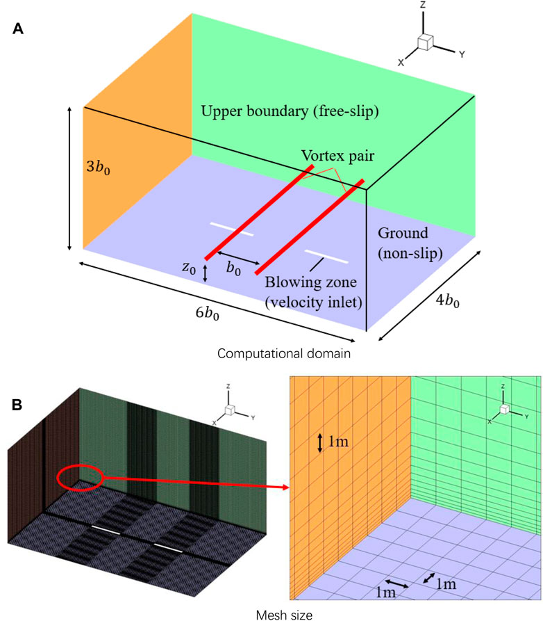
FIGURE 1. Schematic of the computational domain. (A) Computational domain, (B) Mesh size.

The height of the first layer of the mesh near the ground is 0.1 m ($z^{+}\approx 1$) with a growth rate of 1.2, and the mesh size along all three directions are 1 m. Consequently, the total cell numbers for A340 and A380 wake simulations are 12 million and 24 million, respectively. A timestep of $dt$ = 0.01 s was employed in all the simulations, corresponding to a non-dimensional timestep of $3.76\times {10}^{-4}{t}_0$ and $3.35\times {10}^{-4}{t}_0$ for A340 wake and A380 wake, respectively. Besides, 3.4 $t_0$ of wake evolution was simulated in this study, corresponding to 90 s and 102 s for A340 wake and A380 wake, respectively.

The wake vortex pairs were initialised using the Lamb-Oseen model, which describes the velocity field as Equation 3:

$r$ and $r_c$ represent the distance to the vortex center and the vortex core radius, respectively. According to the Class II airport operating standard, the topographic relief height should be less than 1 m within 300 m of the end of the runway. Therefore, the blowing zone is placed 300 m away from the end of the runway. This corresponds to $z_0$ = 31m of the initial wake vortex height [19]. It is highlighted that the non-dimensional initial vortex altitudes for A340 and A380 are different, resulting in a partial non-dimensional optimization in Optimization for Enhanced Wake Vortex Decay section.

Methods Validation

To validate the numerical methods, a numerical simulation was performed and the result was compared with the water-tank experiment data [14]. In the validation, the wake vortex of A340 was employed and the initial vortex height was reduced to $z_0$ = 0.5 $b_0$ to match the experiment setup. Other parameters such as timestep and mesh size remain the same as Boundary and Initial Conditions section.

To evaluate the vortex strength decay history, the vortex centre was tracked by considering the local minimum pressure and the extreme vorticity values first. After that, the vortex circulation on a specify axial plane was obtained by Equation 4:

where ${\displaystyle \underset{0}{\overset{d}{\int }}}\omega dA$ represents the integration of axial vorticity over the circular region with a radius of $d$ [14]. Finally, the circulation values were averaged along several axial planes.

Figure 2 shows the comparison between the CFD result and the experimental data. Before $t^{*}<0.5$, the circulation in the simulation remains constant while the circulation in the experiment exhibits a slow growth. This is due to the roll-up process of the vorticity sheet generated by the wing model, even though the circulation curve of CFD shows similar trend after $t^{*}=1$ and agrees with the experiment data well. Thus, current numerical methods will be adopted in following studies.

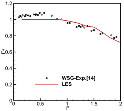
FIGURE 2. Vortex circulation evolution, CFD vs. Exp.

Optimization Method

Kriging Surrogate Model

Surrogate models, also known as response surface models, are approximate mathematical tools used as an alternative to complex numerical analysis, which reduce the difficulty of the optimization process. By learning from the sample data, the computer trains and fits a function mapping the relationship between the design parameters and the corresponding objective values that satisfy a certain accuracy range [21, 22]. The upper and lower bounds of the design variables $X$ determine the design space, and the initial data set is $X=X_1,X_2,\dots ,X_{np}$, where $np$ is the amount of the design variables, letting the unknown function between the response value $Y$ and the design variables $X$ be Equation 5

In the Kriging surrogate model, the actual function $Y$ is expressed as Equation 6:

$f\left(X\right)$, also written as $\beta$, is acquired with the sample points, it represents the global approximation to the design space; $Z\left(X\right)$ is a random function with a mean of 0 and a variance of ${\sigma }^2$, representing the deviation from the global approximation, its covariance matrix is expressed as Equation 7:

$\mathit{R}$ is the correlation matrix. $i=1,2,3\dots n_s$ represents the number of the samples. The Gauss function was chosen as the correlation function, $R$. The estimation of response value $Y\left(X\right)$ at an arbitrary point $X$ is given by Equation 8:

The superscript $T$ means the transposition of a matrix. $r^T$ is the correlation vector between $X$ and the sample points, $\widehat{\beta }$ and $\widehat{\sigma }$ are expressed as Equations 9, 10:

and

Infill-Sampling Criteria

A parallel infill-sampling criteria combing two criteria was used to better approximate the real function. The first criterion, minimizing surrogate prediction (MSP), selects the minimum of the objective function obtained by the current surrogate model as the new sample point [23, 24]. The MSP sub-optimization problem with constraints can be written as Equation 11

$\widehat{g_i}$ is the constraint function, and $n_c$ is the number of constraints. The subscripts, $l$ and $u$, represent the lower bound and upper bound, respectively.

The second infill-sampling criteria, expected improvement (EI), is also known as the efficient global optimization algorithm [25]. The standard EI function can be written as Equation 12:

$Y_{\mathit{min}}$ is the current minimum of the objective function. Suppose the function values predicted by the model at the measured points follow a normal distribution, then $\widehat{Y}$ is the predicted mean value, and $s\left(X\right)$ is the standard deviation. Φ and ϕ are standard normal distribution function and standard normal distribution probability density function, respectively.

In this study, the gradient optimization is combined with the Kriging surrogate model to conduct the optimization process. To be specific, the optimization process consists of the following steps:

1) initial sample points are chosen with the Latin hypercube sampling method and the functional responses are evaluated by CFD solver;

2) initial surrogate models for the objective and constraint functions are constructed based on the current samples;

3) parallel infill-sampling criteria combing the EI and MSP criterion is conducted to obtain new sample points, and the corresponding response values are obtained using CFD;

4) the surrogate model is updated, and the sub-optimization process is performed based on it;

5) steps 3 and 4 are repeated until the termination condition is satisfied.

Benchmark Analytical Test Cases

To validate the above-mentioned optimization framework, three analytical test cases were used.

Rosenbrock Test Case

The Rosenbrock function has a minimum that lies in a “flat valley” (Figure 3C), around which the gradient value is small [24]. Thus, this case assessed the local optimization capability of the algorithm. The Rosenbrock function is expressed as Equation 13:

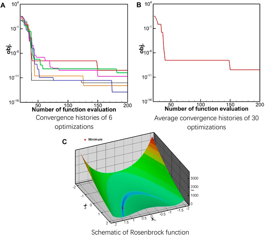
FIGURE 3. Rosenbrock function and the convergence history. (A) Convergence histories of 6 optimizations, (B) Average convergence histories of 30 optimizations, (C) Schematic of Rosenbrock function.

The optimization was performed 30 times and Figure 3 shows the convergence histories. In all calculations, when the number of the function evaluations (NFE) reaches 100, the predicted minimum of the function drops to the order of ${10}^{-8}$, and when NFE is 200, the predicted minimum of the function drops below ${10}^{-10}$. In particular, the best predicted value is close to ${10}^{-14}$, which proves that the algorithm performs well in local optimization problems.

Rastrigin Test Case

Rastrigin function is written as [22] Equation 14:

The optimal solution of the Rastrigin function is $f\left(0,0\right)=0$, while there exist multiple minima in the feasible region (Figure 4C). For instance, in other positions such as $\left(1,0\right)$, $\left(1,1\right)$, and $\left(2,0\right)$, the minimum values obtained by the function are 1, 2, and 4, respectively. Figure 4A shows the convergence histories of six rounds of optimization. Note the sudden drops in the convergence curves, these imply that the local minimum region of $f\left(0,0\right)$ is found, and only local optimization is needed. However, it must be highlighted that the probing of the global minimum is a random process which might take hundreds of function evaluations. As the average convergence curve in Figure 4B drops to the order of ${10}^{-8}$, all the 30 rounds of optimization end when the global minimum is found, implying that the current algorithm has powerful global optimization capability.

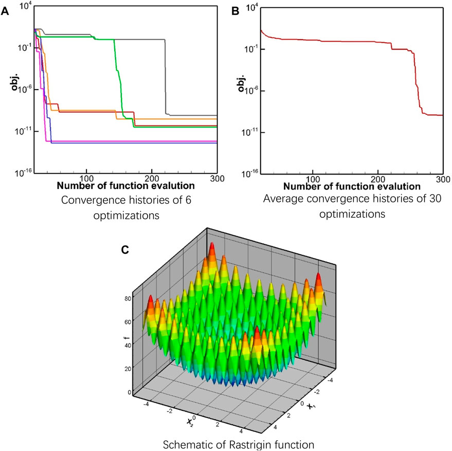
FIGURE 4. Rastrigin function and the convergence history. (A) Convergence histories of 6 optimizations, (B) Average convergence histories of 30 optimizations, (C) Schematic of Rastrigin function.

Constraint Handling Test Case

In this case, two constraints are applied. As shown in Figure 5C, the feasible region is a narrow interval between the constraints, and the minimum of the objective function lies approximately in the middle of the feasible region. The optimization problem is described as [25] Equation 15:

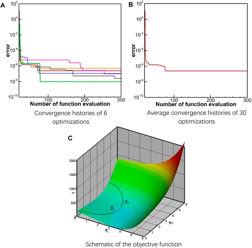
FIGURE 5. Function of test case 3 and the convergence history. (A) Convergence histories of 6 optimizations, (B) Average convergence histories of 30 optimizations, (C) Schematic of the objective function.

Before optimizing, it was checked to ensure that all the initial sample points lie within the feasible region. When using the logarithmic barrier method, the optimization problem can be rewritten as Equation 16:

where $\mu$ = $c{\mu }_0$ is the dynamic penalty factor with $c=0.1$. During the optimization progress, $\mu$ approaches zero gradually, and the unconstrained optimization problem converges to the original constrained optimization problem. Figure 5B shows that before the number of the function evaluations reaches 50, the optimization error has decreased to an order of ${10}^{-5}$. The best result exhibits an error of an order of ${10}^{-8}$ in Figure 5A.

In summary, the current algorithm combing the Kriging surrogate model and the gradient optimization method is able to deal with both constrained and unconstrainted problems, and will be used for the subsequent study.

Optimization for Enhanced Wake Vortex Decay

Before the optimization, the enhancement of wake vortex decay by active flow control method will be introduced briefly. Two rectangular blowing zones were equipped symmetrically about the runway central line, at the end of the runway. When air flows (blowing) vertically from the blowing zones, starting vortices are generated at the edges of the rectangular zones. At the same time, secondary vortices are induced and roll up inhomogeneously, due to the presence of the blowing air. Naturally, these vortical structures interact and develop into a hairpin like vortex ($\mathrm{\Omega }$ vortex) and loop around the primary vortex fast. Under the self-induction effect, the vortex loop extends along the flight direction, interacting with the primary vortex intensely and leading to rapid dissipation of the aircraft wake vortex [18]. It is highlighted that the blowing process was modelled by applying velocity boundary conditions at the blowing zones to simplify the simulation. Therefore, the depth of the blowing zone was not considered. The definition of a blowing zone could be found in Figure 7, the aspect ratio is defined as AR = length/width, where width = area/length. It was found that the blowing effect is improved by an increasing blowing velocity and blowing zone area [18]. Therefore, it is believed that the optimization on blowing velocity and zone area is not necessary. In this study, the blowing zone area was fixed at ${0.04b}_0^2$, and blowing velocity of ${\omega }_0$ was adopted [18].

The wake vortex of A340 is considered in this section, the detailed vortex parameters are listed in Table 1, and the initial vortex altitude is $z_0^{*}=0.654$ ($z_0=31$ m). The time step of the simulation is 0.01s ($3.76\times {10}^{-4}{t}_0$) and 90s (3.4 $t_0$) of wake evolution is simulated. The blowing zone area is ${0.04b}_0^2=89.87{\mathrm{m}}^2$, and the blowing velocity is ${\omega }_0=1.7796$ m/s. With a fixed blowing area, the parameters that affect the enhancement are blowing zone aspect ratio (AR, determined by the blowing zone length) and blowing zone position (P). Thus, our aim in this section is to find the optimum selection of AR and P and obtain the best enhancement effect.

Vortex circulation at an axial position is generally used to evaluate the vortex strength. However, instantaneous circulation is affected by many random factors and is unrepresentative for the entire wake decay process. Therefore, the vortex strengths at $x^{*}=0$, $x^{*}=1$, and $x^{*}=2$ (defined in Figure 7) are considered comprehensively.

Taking the case 1 in reference [19] as an example, as shown in Figure 6, the shadow area ${\mathrm{\Gamma }}_{\mathrm{s}}$ reflects the mean circulation in the entire simulation process. For the $x^{*}=0$ section, smaller ${\mathrm{\Gamma }}_{\mathrm{s}}$ indicates lower local vortex strength after the rapid decay. For $x^{*}=1$ and $x^{*}=2$ sections, smaller ${\mathrm{\Gamma }}_{\mathrm{s}}$ corresponds to an earlier beginning of the rapid decay, which reflects the higher extension velocity and stronger intensity of the helical vortices. Therefore, the objective function of the optimization can be expressed as Equation 17:

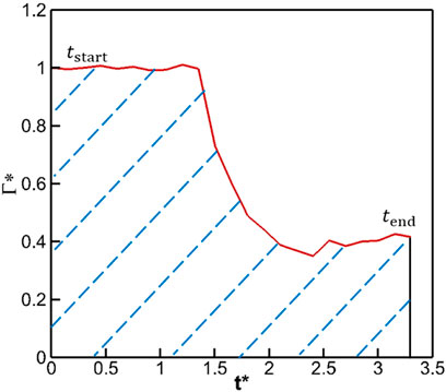
FIGURE 6. Circulation history of case 1 in reference [19].

During the simulation, the flow field data is logged at 4s interval, and thus, the objective function can be simplified as Equation 18:

where $i$ is the $i$ th instant and $N$ is the total number of recorded instants. Since both circulation and time are non-dimensionalized, the objective function is also a non-dimensional value. Figure 7 demonstrates the two parameters considered in the optimization. The blowing zone length $X_1$ restricts the aspect ratio, and the distance between the centre of the blowing zone and the central axis, $X_2$, defines the blowing position. If the boundaries of the blowing zone could not exceed the computational domain boundaries, the constraints for the optimization can be expressed as Equation 19:

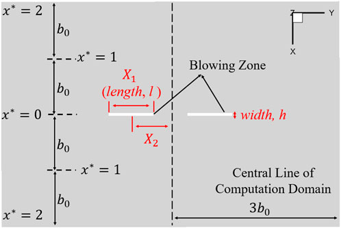
FIGURE 7. Definition of the optimization parameters (bottom of the computational domain).

It must be noted that the response value for every new sample point is evaluated by CFD, which may consume more than 20 h when using a 64 cores server. The automated process is as follows (Figure 8):

1) for a new sample point, the batch file is generated according to the input design parameters; then, the structured mesh is generated using the batch files in ICEM CFD;

2) the CFD simulation is conducted using ANSYS FLUENT, in which the .jou file controls the CFD simulation details such as timestep and turbulence modelling etc.;

3) the flow field information is extracted and post-processed using an in-house code to get the objective function value;

4) the new sample point parameter and corresponding objective function value is transferred to update the surrogate model;

5) another round of sample infilling is conducted if necessary.

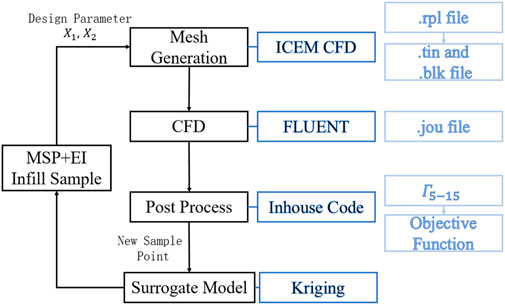
FIGURE 8. Processes for new sample evaluation.

Considering the high cost of the CFD, two termination conditions are employed:

1) the total number of samples exceeds 210 ($n_{\text{sample}}\ge 210$)

2) the error of the adjacent two iterations is smaller than ${10}^{-5}$

As shown in Figure 9A, the optimal design of the current problem is found at the 20th sample point, while none of the subsequent sample points show a significant decrease in the objective function value. The better designs are concentrated around obj. = 11. Nevertheless, as the number of sample points increases, the surrogate model gradually stabilizes, and the adjacent error of the optimal value found by the surrogate model exhibits an overall decreasing trend. At the end of the optimization, the adjacent decreases to the order of ${10}^{-5}$ (Figure 9B).

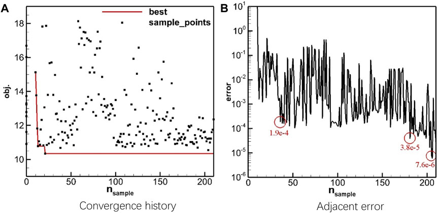
FIGURE 9. Convergence history of blowing zone optimization. (A) Convergence history, (B) Adjacent error.

Figure 10 illustrates the modelling when the error of the optimal value decreases to the order of ${10}^{-3}$, ${10}^{-4}$, and ${10}^{-5}$ for two adjacent iterations. Figures 10A, C, E are coloured using the objective function values, obj., while Figures 10B, D, F are coloured using the EI values. Above the black dashed line in the figures is the feasible domain. When $n_{\text{sample}}=36$, the max of the EI values in the feasible domain is less than 0.1, indicating that the surrogate model already has high credibility. The response surface of $n_{\text{sample}}=36$ is close to that of $n_{\text{sample}}=181$, lower obj. value is observed in the middle of the design space. It is observed that in most of the region of $x_1\in \left[0.1b_0,1b_0\right]$ and $x_2\in \left[0.5b_0,1.1b_0\right]$, obj. is smaller than 12, and in the neighbouring region of $x_1$ = 0.3 $b_0$ and $x_2$ = 0.8 $b_0$, obj. is smaller than 11. When $n_{\text{sample}}$ is increased to 205, EI values decrease further throughout the region while there is only limited change to the response surface, implying that the current surrogate model has converged and is reliable.

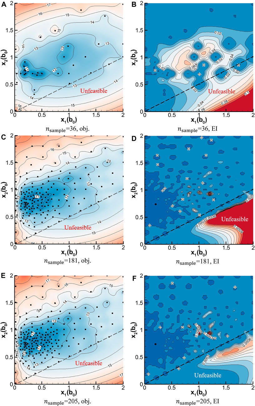
FIGURE 10. Response surface and EI contour. (A) $n_{\text{sample}}=36$ obj, (B) $n_{\text{sample}}=36$ EI, (C) $n_{\text{sample}}=181$ obj, (D) $n_{\text{sample}}=181$ EI, (E) $n_{\text{sample}}=205$ obj, (F) $n_{\text{sample}}=205$ EI.

Figures 11–17 exhibit the vortex structures of two initial sample cases, four infilled sample cases, and the best performing sample case during the optimization. All the relative positions in the design space are shown in Figure 18, the design parameters are shown in Table 2, and the circulation decay histories are exhibited in Figure 19.

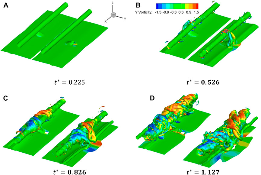
FIGURE 11. Structures of initial sample 1. (A) $t^{*}=0.225$, (B) $t^{*}=0.526$, (C) $t^{*}=0.826$, (D) $t^{*}=1.127$.

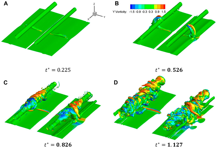
FIGURE 12. Structures of initial sample 2. (A) $t^{*}=0.225$, (B) $t^{*}=0.526$, (C) $t^{*}=0.826$, (D) $t^{*}=1.127$.

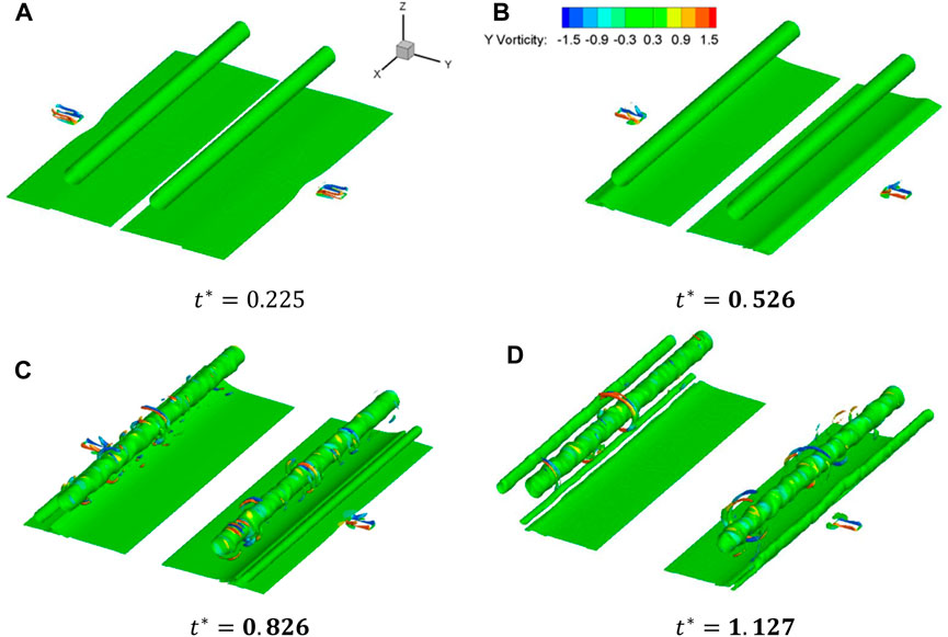
FIGURE 13. Structures of sample 70. (A) $t^{*}=0.225$, (B) $t^{*}=0.526$, (C) $t^{*}=0.826$, (D) $t^{*}=1.127$.

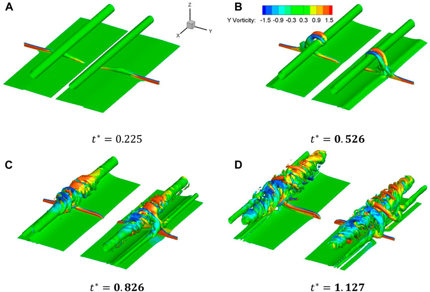
FIGURE 14. Structures of sample 73. (A) $t^{*}=0.225$, (B) $t^{*}=0.526$, (C) $t^{*}=0.826$, (D) $t^{*}=1.127$.

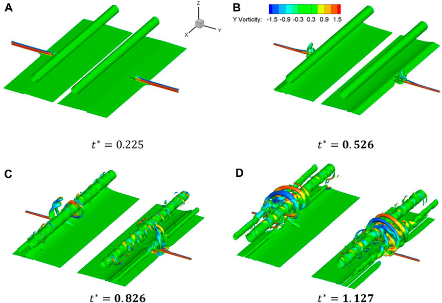
FIGURE 15. Structures of sample 76. (A) $t^{*}=0.225$, (B) $t^{*}=0.526$, (C) $t^{*}=0.826$, (D) $t^{*}=1.127$.

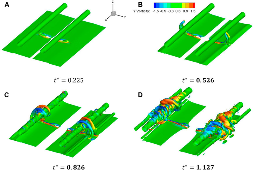
FIGURE 16. Structures of sample 150. (A) $t^{*}=0.225$, (B) $t^{*}=0.526$, (C) $t^{*}=0.826$, (D) $t^{*}=1.127$.

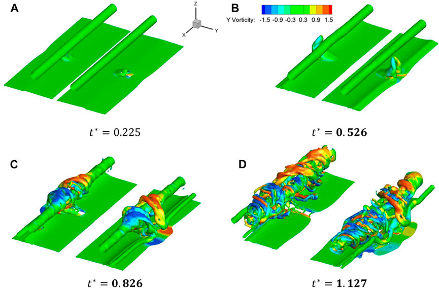
FIGURE 17. Structures of the optimal sample. (A) $t^{*}=0.225$, (B) $t^{*}=0.526$, (C) $t^{*}=0.826$, (D) $t^{*}=1.127$.

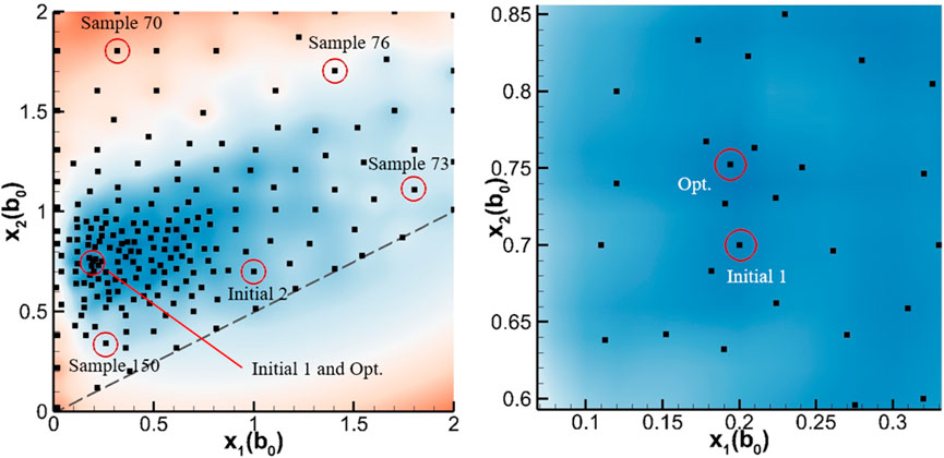
FIGURE 18. Samples to be demonstrated.

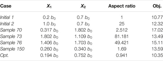
TABLE 2. Design parameters of initial samples and the best performing sample.

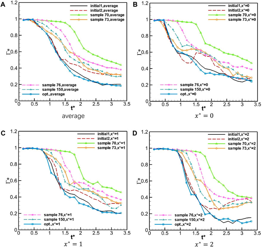
FIGURE 19. Circulation history at different axial positions (seven cases). (A) average, (B) ${\mathrm{x}}^{*}=0$, (C) ${\mathrm{x}}^{*}=1$, (D) ${\mathrm{x}}^{*}=2$.

Take sample cases 76 and 150 as examples. The $\mathrm{\Omega }$ vortex in Sample 73 has already had contact with the primary vortex at $0.526t_0$; and at $1.127t_0$, the helical vortex has already reached the boundaries of the computational domain. By comparison, the helical vortex just reached $x^{*}=1$ at $1.127t_0$. Figure 19 also shows that at different positions, the rapid decay in Sample 150 sets off later than that in Sample 73. It is noted that the slope of the circulation curves at $x^{*}=1$ and $x^{*}=2$ of Sample 150 are steeper than those in Sample 73. This is because the blowing zone in Sample 150 has a smaller length ($X_1$) and larger width, which produces a stronger starting vortex and more intense interaction on the aircraft wake vortex [16]. Sample 70 is an exception of the above cases. Since the blowing zone is far from the centre line ($X_2=1.802b_0$) and the length of the blowing zone is small ($X_1=0.317b_0$), the blowing airflow never effectively interferes with the secondary vortex, and eventually the primary vortex simply undergoes a natural dissipation process. At $t^{*}=1.127$, the primary vortex structure still remains intact (Figure 13), and the rapid decay in Sample 76 sets off late. Figure 15B shows that the $\mathrm{\Omega }$ vortex forms at $0.526t_0$. As a result, the wake decay enhancement of Sample 76 is only better than that of Sample 70.

The vortex structures in the two initial sample cases and the best performing case are similar. Considering the induced lateral movement of the IGE vortex, a large value of $X_2=0.7b_0$ is selected for the two initial sample cases [19]. Since the starting vortex interacts with the wake vortex at $x^{*}=0$ directly, the local circulation in these three cases drops fast at 0.45 $t_0$. At least until 0.9 $t_0$, the blowing zone aspect ratio does not obviously affect accelerated wake dissipation. However, due to the weak starting vortex, the circulation in case Initial 2 experienced a rebound between $1<t^{*}<2.5$. At $x^{*}=1$ and $x^{*}=2$, the local rapid decay in Initial 2 sets off later than those in other two cases, which is also the consequence of the weak starting vortex. The helical vortex in Initial 2, developed from the starting vortex, extends slower and affects the wake vortex to a limited extension. Compared with Initial 1, the design parameters and vortex decay history in Opt. is similar. It is noticed that, although the starting vortex in Opt. is relatively weak, due to the influence of the blowing zone position, the circulation in Opt. is lower after the rapid decay phase.

Overall, the vortex evolutions in most cases are similar: a) the starting vortex generated by blowing air is raised by the blowing air and primary vortex induction b) the starting vortex evolves into a hairpin vortex ($\mathrm{\Omega }$ vortex) and interacts with the primary vortex c) $\mathrm{\Omega }$ vortex loops around the primary vortex and extends along the x direction. The main difference between different cases is the timing and intensity of the above processes. From Figure 10E, the surrogate model shows that the best performing setting for A340 wake decay enhancement is $X_1=0.194b_0,X_2=0.752b_0$. Since the blowing zone area is fixed to ${0.04b}_0^2$, it is obtained that the blowing zone aspect ratio is close to 1. Besides, in the range of $X_1\in \left[0.1b_0,1b_0\right]$ and $X_2\in \left[0.5b_0,1.1b_0\right]$, the objective function is smaller than 12, which is still a considerable enhancement for wake vortex decay.

Multi-Objective Design

The optimum blowing zone for an A340 wake vortex pair may not be enough to destroy the wake of a heavier aircraft, such as an A380, within a short period. Therefore, a better design could be obtained by overlapping the design space of two blowing zone types, which are for different aircraft wake decay enhancements, respectively. Taking the above optimization result as an example, Figure 10E can be dimensionalized using A340 and A380 parameters (Table 3). It is highlighted that the optimization process in the previous section is partially dimensionless. Since the initial vortex altitude of $z_0=31\mathrm{m}$ during the landing phase applies for all types of aircrafts, the dimensionless altitude for aircrafts with different wingspans varies in a certain range. Therefore, the final selection of design parameters should be based on the characteristic parameters of the aircraft with the largest wingspan, which is taken as the characteristic parameters of A380 in the present study. The basis for this selection is:

1) for A380 (aircraft with larger span), the dimensionless initial altitude is less than that used in the optimization;

2) for A340 (aircraft with shorter span), the dimensionless blowing area is larger than that used in the optimization.

TABLE 3. Parameters for different wake simulations.

These two facts ensure that the simulated blowing effect is not worse than that predicted by the surrogate model.

The design space is divided by the contour lines of the response surface (objective function), the value of the objective function inside the contour lines is smaller than that of the objective function on the contour lines. Figure 20 shows the contour lines on which the objective function equals 11.5. When the design parameters inside the blue contour line (${\mathrm{D}}_{340}$) are used, the objective function of A340 wake vortex is smaller than 11.5. The critical value of 11.5 is chosen because it already corresponds to an impressive enhancement on wake vortex decay. The intersection region of ${\mathrm{D}}_{380}$ and ${\mathrm{D}}_{340}$ (shadow zone) represents the optimum design space (${\mathrm{D}}_{\text{opt}}$), with which the blowing process is most effective for both A340 wake and A380 wake. Considering that a longer blowing zone improves the blowing effect [19], the final selection of the design, $X_1=43\mathrm{m}$ and $X_2=47.5\mathrm{m}$, is close to the right boundary of ${\mathrm{D}}_{\text{opt}}$. According to the parameters of the A380 wake, the width of the blowing zone is $h={\left(0.2\times 62.6\right)}^2/43\mathrm{m}=3.65\mathrm{m}$.

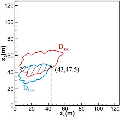
FIGURE 20. Design space of blowing zone for different aircraft wake vortex (Opt. < 11.5).

Two simulations are performed to validate the optimization results. For A340 and A380 wake vortex simulations, the same non-dimensional computation domain ($4{\mathrm{b}}_0\times {6\mathrm{b}}_0\times 3{\mathrm{b}}_0$) and non-dimensional blowing velocity (${\omega }_0$) are employed, meaning that the absolute computational domain and blowing velocity are different. But the blowing areas are exactly the same as the above optimized result ($x_1=43\mathrm{m}$, $x_2=47.5\mathrm{m}$ and $h=3.65\mathrm{m}$). It is noted that for A380 wake simulation, the timestep is 0.01s ($3.35\times {10}^{-4}{t}_0$) and 102s (3.4 $t_0$) of wake evolution is simulated. The blowing zone area is ${0.04b}_0^2=156.75{\mathrm{m}}^2$, and the blowing velocity is ${\omega }_0=2.0975$ m/s.

Figure 21 and Figure 22 show the wake vortex structures of A340 and A380 under the blowing effect. Due to the large initial circulation of the A380 wake vortex, the starting vortex experiences high induced velocity and is raised quickly. Figure 22B shows that a vortex loop is evolved from the $\mathrm{\Omega }$ vortex at $t=14\mathrm{s}$ in the case of A380 case, while in the case of A340, the $\mathrm{\Omega }$ vortex has just formed and approached the primary vortex. After that, under the self-induction, the vortex loop extends along the x direction and forms helical vortices, which destruct the wake vortex structures rapidly. It is noted that at $t=22\mathrm{s}$, the helical vortices in the case of A380 develop faster than that in the case of A340, implying that the interference between the primary vortex and the blowing induced structures is more intense in the case of A380.

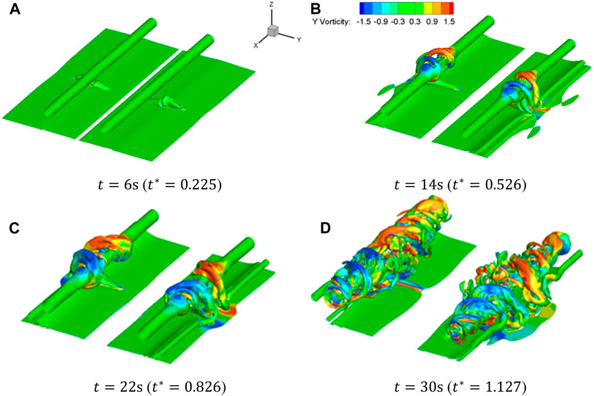
FIGURE 21. Structures of A340 wake vortex (coloured by y vorticity 1/s). (A) $\mathrm{t}=6\mathrm{s}$ (${\mathrm{t}}^{*}=0.225$), (B) $\mathrm{t}=14\mathrm{s}$ (${\mathrm{t}}^{*}=0.526$), (C) $\mathrm{t}=22\mathrm{s}$ (${\mathrm{t}}^{*}=0.826$), (D) $\mathrm{t}=30\mathrm{s}$ (${\mathrm{t}}^{*}=1.127$).

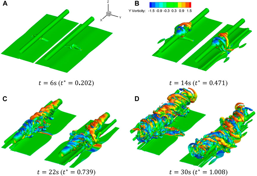
FIGURE 22. Structures of A380 wake vortex (coloured by y vorticity 1/s). (A) $t=6\mathrm{s}$ ($t^{*}=0.202$), (B) $t=14\mathrm{s}$ ($t^{*}=0.471$), (C) $t=22\mathrm{s}$ ($t^{*}=0.739$), (D) $t=30\mathrm{s}$ ($t^{*}=1.008$).

Figure 23 shows the decay history of the A340 and A380 wake vortex with optimized blowing zones. Due to the interference of the starting vortex, the rapid decay of the A340 wake vortex is brought approximately 1.5 $t_0$ ahead by blowing. At $t^{*}=3.3$, the average circulation of the A340 wake with blowing decreases to 0.15, which is much lower than that of the baseline case. The initial dimensionless altitude of the A380 wake vortex is smaller than 0.5, resulting in a better blowing effect. Consequently, the rapid decay sets off at 0.2 $t_0$ in the blowing case. The objective function values for the A340 and A380 cases are 11.12 and 10.19, respectively. With the current blowing zone settings, the wake vortex decay for both aircraft types is enhanced and reaches the design objective (objective function < 11.5).

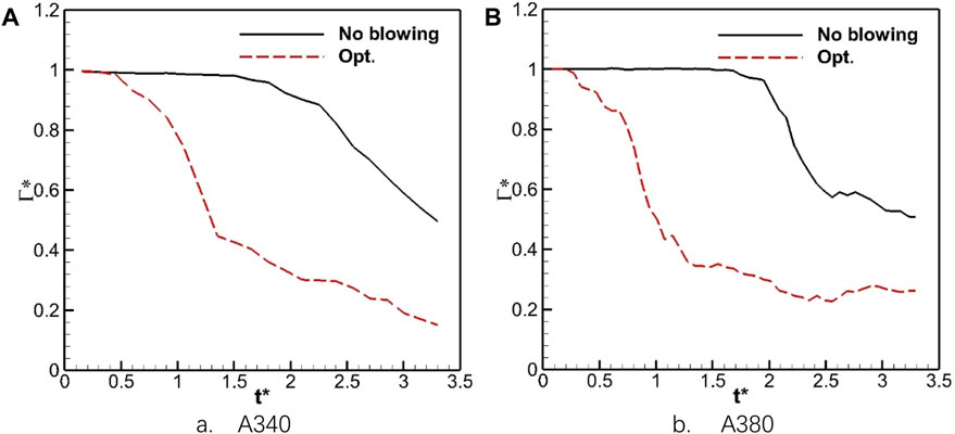
FIGURE 23. Averaged circulation histories for different aircraft wakes with optimized blowing zones. (A) A340, (B) A380.

Conclusion

In this paper, the Kriging surrogate model is used to help obtain a better design of the blowing zone for enhancement of wake vortex decay. By overlapping and comparing the design spaces for different wake vortices, a multi-objective design is realized, which improves the engineering feasibility of the current blowing method. The main findings are as follows:

1. The current optimization algorithm combing Kriging surrogate model and gradient optimization algorithm deal with the global optimization problems and constrained problems well;

2. The blowing effect is non-linearly related to the blowing zone aspect ratio and position. The blowing zone should not be too close to the centre of the computational domain and the blowing zone aspect ratio should be close to 1;

3. For the A340 wake vortex with an initial altitude of $z=31\mathrm{m}$ ($z^{*}=0.654$), the objective function is smaller than 12 in the range of $X_1\in \left[0.1b_0,1b_0\right]$ and $X_2\in \left[0.5b_0,1.1b_0\right]$, and the best performing setting is $X_1=0.194{\mathrm{b}}_0$, $X_2=0.752{\mathrm{b}}_0$;

4. By overlapping the design spaces, an optimized blowing zone, which enhances the decay of A340 and A380 wake vortex, is founded. Numerical simulation proves this blowing zone effective and reduces the objective function to 11.12 and 10.19 for the different wake vortices, respectively.

Data Availability Statement

The original contributions presented in the study are included in the article/Supplementary Material, further inquiries can be directed to the corresponding author.

Author Contributions

ZX (the first author) was responsible for numerical simulations, data processing and manuscript writing. DL (the second author) was responsible for the conceptual design of the study, funding support and the manuscript review. All authors contributed to the article and approved the submitted version.

Conflict of Interest

The authors declare that the research was conducted in the absence of any commercial or financial relationships that could be construed as a potential conflict of interest.

References

1. Gerz, T, Holzäpfel, F, and Darracq, D. Commercial Aircraft Wake Vortices. Prog Aerospace Sci (2002) 38(3):181–208. doi:10.1016/s0376-0421(02)00004-0
2. Holzäpfel, F, Tchipev, N, and Stephan, A. Wind Impact on Single Vortices and Counterrotating Vortex Pairs in Ground Proximity. Flow Turbulence and Combustion (2016) 97(3):829–48. doi:10.1007/s10494-016-9729-2
3. Xu, Z, Li, D, and Cai, J. Long-Wave Deformation of In-Ground-Effect Wake Vortex Under Crosswind Condition. Aerospace Sci Tech (2023) 142:108697. doi:10.1016/j.ast.2023.108697
4. ICAO. ICAO DOC 4444 Air Traffic Management - Procedures for Air Navigation Services (PANS-ATM). 16. Montréal, Quebec, Canada: ICAO (2016).
5. Holbrook, GT, Dunham, DM, and Greene, GC. Vortex Wake Alleviation Studies With a Variable Twist Wing. Technical Paper 2442. Hampton, Virginia, United States: NASA (1985).
6. Breitsamter, C. Wake Vortex Characteristics of Transport Aircraft. Prog Aerospace Sci (2011) 47(2):89–134. doi:10.1016/j.paerosci.2010.09.002
7. Ruhland, J, Heckmeier, FM, and Breitsamter, C. Experimental and Numerical Analysis of Wake Vortex Evolution Behind Transport Aircraft With Oscillating Flaps. Aerospace Sci Tech (2021) 119:107163. doi:10.1016/j.ast.2021.107163
8. Breitsamter, C, and Allen, A. Transport Aircraft Wake Influenced by Oscillating Winglet Flaps. J Aircraft (2009) 46(1):175–88. doi:10.2514/1.37307
9. Cheng, Z, Wu, Y, Xiang, Y, Liu, H, and Wang, FX. Benefits Comparison of Vortex Instability and Aerodynamic Performance From Different Split Winglet Configurations. Aerospace Sci Tech (2021) 119:107219. doi:10.1016/j.ast.2021.107219
10. Rennich, SC, and Lele, SK. Method for Accelerating the Destruction of Aircraft Wake Vortices. J Aircraft (1999) 36(2):398–404. doi:10.2514/2.2444
11. Stumpf, E. Study of Four-Vortex Aircraft Wakes and Layout of Corresponding Aircraft Configurations. J Aircraft (2005) 42(3):722–30. doi:10.2514/1.7806
12. Cho, J, Lee, BJ, Misaka, T, and Yee, K. Study on Decay Characteristics of Vertical Four-Vortex System for Increasing Airport Capacity. Aerospace Sci Tech (2020) 105:106017. doi:10.1016/j.ast.2020.106017
13. Kohl, RE. Model Experiments to Evaluate Vortex Dissipation Devices Proposed for Installation on or Near Aircraft Runways. Hampton, Virginia, United States: NASA (1973).
14. Stephan, A, Holzäpfel, F, Misaka, T, Geisler, R, and Konrath, R. Enhancement of Aircraft Wake Vortex Decay in Ground Proximity: Experiment Versus Simulation. CEAS Aeronaut J (2013) 5(2):109–25. doi:10.1007/s13272-013-0094-8
15. Holzäpfel, F, Stephan, A, Rotshteyn, G, Körner, S, Wildmann, N, Oswald, L, et al. Mitigating Wake Turbulence Risk During Final Approach Via Plate Lines. AIAA J (2021) 2021:59. doi:10.2514/6.2020-2835
16. Xu, Z, Li, D, An, B, and Pan, W. Enhancement of Wake Vortex Decay by Air Blowing From the Ground. Aerospace Sci Tech (2021) 118:107029. doi:10.1016/j.ast.2021.107029
17. Xu, Z, and Li, D. Enhanced Aircraft Wake Decay Under Crosswind Conditions. J Aircraft (2023) 60(5):1687–99. doi:10.2514/1.C037127
18. Misaka, T, Holzäpfel, F, Hennemann, I, Gerz, T, Manhart, M, and Schwertfirm, F. Vortex Bursting and Tracer Transport of a Counter-Rotating Vortex Pair. Phys Fluids (2012) 24(2):25104. doi:10.1063/1.3684990
19. Han, Z, Chen, J, Zhang, K, Xu, ZM, Zhu, Z, and Song, WP. Aerodynamic Shape Optimization of Natural-Laminar-Flow Wing Using Surrogate-Based Approach. AIAA J (2018) 56(7):2579–93. doi:10.2514/1.j056661
20. Han, Z. SURROOPT: A Generic Surrogate-Based Optimization Code for Aerodynamic and Multidisciplinary Design. In: 30th Congress of the International Council of the Aeronautic Sciences (2016).
21. Sasena, MJ, Papalambros, P, and Goovaerts, P. Exploration of Metamodeling Sampling Criteria for Constrained Global Optimization. Eng optimization (2002) 34(3):263–78. doi:10.1080/03052150211751
22. Parr, JM, Keane, AJ, Forrester, AIJ, and Holden, CM. Infill Sampling Criteria for Surrogate-Based Optimization With Constraint Handling. Eng optimization (2012) 44(10):1147–66. doi:10.1080/0305215x.2011.637556
23. Jones, DR, Schonlau, M, and Welch, WJ. Efficient Global Optimization of Expensive Black-Box Functions. J Glob optimization (1998) 13(4):455–92. doi:10.1023/a:1008306431147
24. Rosenbrock, HRH. An Automatic Method for Finding the Greatest or Least Value of a Function. Comp J (1960) 3(3):175–84. doi:10.1093/comjnl/3.3.175
Keywords: active flow control, aircraft wake vortex, multi-objective design, Kriging, CFD
Citation: Xu Z and Li D (2024) Numerical Optimization on Aircraft Wake Vortex Decay Enhancement. Aerosp. Res. Commun. 2:12444. doi: 10.3389/arc.2024.12444
Received: 19 November 2023; Accepted: 05 January 2024;
Published: 24 January 2024.
Copyright © 2024 Xu and Li. This is an open-access article distributed under the terms of the Creative Commons Attribution License (CC BY). The use, distribution or reproduction in other forums is permitted, provided the original author(s) and the copyright owner(s) are credited and that the original publication in this journal is cited, in accordance with accepted academic practice. No use, distribution or reproduction is permitted which does not comply with these terms.
*Correspondence: Dong Li, ldgh@nwpu.edu.cn