New Optical Solutions of the Fractional Gerdjikov-Ivanov Equation With Conformable Derivative

Ghanbari, Behzad; Baleanu, Dumitru

doi:10.3389/fphy.2020.00167

ORIGINAL RESEARCH article

Front. Phys., 15 May 2020
Sec. Statistical and Computational Physics
Volume 8 - 2020 | https://doi.org/10.3389/fphy.2020.00167

New Optical Solutions of the Fractional Gerdjikov-Ivanov Equation With Conformable Derivative

Behzad Ghanbari^1,2^*

Dumitru Baleanu^3,4,5

¹Department of Engineering Science, Kermanshah University of Technology, Kermanshah, Iran
²Department of Mathematics, Faculty of Engineering and Natural Sciences, Bahçeşehir University, Istanbul, Turkey
³Department of Mathematics, Faculty of Arts and Sciences, Cankaya University, Ankara, Turkey
⁴Institute of Space Sciences, Magurele-Bucharest, Romania
⁵Department of Medical Research, China Medical University Hospital, China Medical University, Taichung, Taiwan

Finding exact analytic solutions to the partial equations is one of the most challenging problems in mathematical physics. Generally speaking, the exact solution to many categories of such equations can not be found. In these cases, the use of numerical and approximate methods is inevitable. Nevertheless, the exact PDE solver methods are always preferred because they present the solution directly without any restrictions to use. This article aims to examine the perturbed Gerdjikov-Ivanov equation in an exact approach point of view. This equation plays a significant role in non-linear fiber optics. It also has many important applications in photonic crystal fibers. To this end, firstly, we obtain some novel optical solutions of the equation via a newly proposed analytical method called generalized exponential rational function method. In order to understand the dynamic behavior of these solutions, several graphs are plotted. To the best of our knowledge, these two techniques have never been tested for the equation in the literature. The findings of this article may have a high significance application while handling the other non-linear PDEs.

1. Introduction

Non-linear Schrödinger equations (NLSE) are often studied from different points of view. In recent years a great variety of analytical and numerical methods have been proposed for solving these equations [1–4]. The most studied NLSE equation is that which has a cubic non-linearity. In the present paper, we will explore an NLSE that has a quintic non-linearity, namely the perturbed Gerdjikov-Ivanov (pGI) equation.

The main achievement of this research is to utilize a new method to derive some novel solutions to a variant form of NLSE. In particular, we consider the pGI equation is given by [5–11]

\begin{array}{l} i \frac{\partial q}{\partial t} + a \frac{\partial^{2} q}{\partial x^{2}} + b | q |^{4} q = i [c q^{2} \frac{\partial \bar{q}}{\partial x} + λ_{1} \frac{\partial q}{\partial x} + λ_{2} \frac{\partial (| q |^{2} q)}{\partial x} + θ \frac{\partial | q |^{2}}{\partial x} q], & (1) \end{array}

provided that q(x, t) indicates the macroscopic complex-valued wave profile of temporal and spatial independent variables of t and x, respectively. In this equation, ∂q/∂t is linear temporal evolution, ∂²q/∂x² stands for the group velocity dispersion (GVD), and |q|⁴q is the present quintic non-linearity of the model. The parameters a, b are the coefficients of these quantities, respectively. Moreover c is the non-linear dispersion coefficient. Finally, the constants λ₁, λ₂, and θ are known parameters related to perturbative effects. More information on this model can be found in the references as mentioned earlier.

In recent years, because of its high importance, the model has attracted the attention of many researchers. For instance, Biswas and Alqahtani [6] have presented two varieties of bright soliton solutions by the use of the semi-inverse variational principle. The sine-Gordon equation approach has been used to extract the dark, bright, dark-bright, singular, and combined singular optical solitons of the equation in Yaşar et al. [7]. Biswas et al. [8] have retrieved some bright and singular optical soliton solutions to the pGI equation by the implementation of the extended trial equation method. The exp(ϕ(ξ))-Expansion and the Kudryashov methods are two reliable techniques that have been used in Arshed [9] to investigate some solitary wave solutions of the equation. In Kaur and Wazwaz [10], several hyperbolic, trigonometric or rational function solutions have been proposed using two efficient techniques, namely exp(ϕ(ξ))-Expansion and $\frac{G^{'}}{G^{2}}$ -expansion methods. Very recently, Hosseini et al. [11] have listed several Kink, bright, and dark optical solitons of the model by the aid of the exp_a-function method and a new version of the Kudryashov method.

In light of previous work, we will apply the generalized exponential rational function method (GERFM) to retrieve some new analytical optical solutions of the fractional pGI equation with the conformable derivative [12]. This new definition of derivative is based on the basic limit definition of the derivative that has been successfully tackled in solving many different problems [13–22]. The main structure of the present article is as outlined. In the second section of this paper, some mathematical preliminaries have been reviewed. This section includes the necessary steps of applying GERFM, and the definition and basic properties of the conformable derivative will be presented. The main results of this article are achieved by following these steps in section 3 of this contribution. In section 4, we have performed some numerical simulations of the obtained results. These graphs can help us in better understanding of their dynamic properties. Finally, the article concludes with some conclusions.

2. Mathematical Preliminaries and Backgrounds

This section first deals with the structure of the GERFM. Then in the next subsection, the basic concepts of the conformable derivative are expressed.

2.1. Analysis of GERFM

GERFM is a newly developed method introduced by Ghanbari and Inc [23] to solve the resonance non-linear Schrödinger equation [23]. Other successful applications of the technique in solving different types of PDEs have also been reported in references [24–27].

We will review how to use the method below.

1. Let us consider a typical non-linear PDE for q = q(x, t), giving by

\begin{array}{l} N (q, q_{x}, q_{t}, q_{x x}, \dots) = 0 . & (2) \end{array}

Under the wave transformations of q(x, t) = Q(ξ) and ξ = σx − lt, Equation (2) becomes an ordinary differential equation given by:

\begin{array}{l} N (Q, σ Q^{'}, - l Q^{'}, σ^{2} Q^{″}, \dots) = 0 . & (3) \end{array}

2. Now, we assume that Equation (3) admits the exact solution giving by

\begin{array}{l} Q (ξ) = A_{0} + \sum_{k = 1}^{N} A_{k} Φ {(ξ)}^{k} + \sum_{k = 1}^{N} B_{k} Φ {(ξ)}^{- k}, & (4) \end{array}

where

\begin{array}{l} Φ (ξ) = \frac{m_{1} e^{n_{1} ξ} + m_{2} e^{n_{2} ξ}}{m_{3} e^{n_{3} ξ} + m_{4} e^{n_{4} ξ}} . & (5) \end{array}

and m_i, n_i's and $A_{0}, A_{k}$ , and $B_{k}$ 's are disposal parameters. Finally, N is a constant, which is evaluated by applying the homogeneous balance to Equation (3).

3. Inserting Equation (4) into (3) with Equation (5), and then gathering all possible powers of $E_{i} = e^{n_{i} ξ}$ for i = 1, …, 4, forms a polynomial equation as $P (E_{1}, E_{2}, E_{3}, E_{4}) = 0$ . Equating coefficients of P to zero, one derives a simultaneous system of equations regarding m_i, n_i(1 ≤ i ≤ 4), and $σ, l, A_{0}, A_{k}$ and $B_{k} (1 \leq k \leq N)$ .

4. Finally, solving the non-linear system and substituting the obtained solutions in Equations (4) and (5), the explicit form of the solutions of (2) will be extracted.

2.2. The Conformable Derivative

Definition: Let q: ℝ⁺ → ℝ, then the conformable derivative of q of order α, is giving by [12]

\begin{array}{l} D_{t}^{α} (q) (t) = lim_{η \to 0} \frac{q (t + η t^{1 - α}) - q (t)}{η}, α \in (0, 1] . & (6) \end{array}

Theorem: For any α ∈ (0, 1], and two α-differentiable functions p, q, the following propositions hold

• $D_{t}^{α} (c_{1} p + c_{2} q) = c_{1} D_{t}^{α} (p) + c_{2} D_{t}^{α} (q)$ , for c₁, c₂ ∈ ℝ.

• $D_{t}^{α} (t^{c}) = c t^{c - α}$ , for c ∈ ℝ.

• $D_{t}^{α} (p q) = p D_{t}^{α} (q) + q D_{t}^{α} (p)$ .

• $D_{t}^{α} (\frac{p}{q}) = \frac{q D_{t}^{α} (p) - p D_{t}^{α} (q)}{q^{2}}$ .

• If q is a differentiable function (in standard sense), thereupon $D_{t}^{α} (q) (t) = t^{1 - α} \frac{d q}{d t}$ holds.

Theorem [14]: Let p:(0, 1] → ℝ be a function such that p is classical, and α-conformable differentiable. Moreover, consider q as a differentiable function defined in the range of p. Thus, we have

\begin{array}{l} D_{t}^{α} (p o q) (t) = t^{1 - α} q^{'} (t) p^{'} (q (t)), \end{array}

where prime stands for standard derivatives respect to t.

Some of the benefits of the conformable derivative compared to other new definitions for the derivative are as follows:

• According to this definition of the operator, the derivative of a constant function is zero. This feature is not available in many other definitions.

• Unlike many existing definitions, this definition satisfies the known formula of the derivative of the product of two functions.

• The conformable derivative does satisfy the known formula of the derivative of the quotient of two functions.

• The conformable derivative does satisfy the well-known chain rule.

• The conformable derivative satisfies the well-known semi group property.

The mentioned properties are very important and valuable features for any derivative definition that the conformable derivative has all of them.

3. Mathematical Analysis

The main contribution in this paper is to consider the derivatives in the Equation (1) with the conformable derivative defined by (6), as follows

\begin{array}{l} i D_{t}^{α} q + a D_{x}^{2 α} q + b | q |^{4} q = i [c q^{2} D_{x}^{α} \bar{q} + λ_{1} D_{x}^{α} q \\ + λ_{2} D_{x}^{α} (| q |^{2} q) + θ D_{x}^{α} | q |^{2} q] . & (7) \end{array}

The main assumption is to taking the stationary soliton solution form of

\begin{array}{l} q (x, t) = Q (ξ) e^{i ϕ (x, t)}, ξ = (\frac{1}{α}) x^{α} - (\frac{ν}{α}) t^{α}, \\ ϕ = (\frac{- k}{α}) x^{α} + (\frac{ω}{α}) t^{α}, & (8) \end{array}

where ν, k, and ω are the phase component, the frequency of solitons, and the wavenumber, respectively.

Substituting the stationary soliton solution form (8) into Equation (7), we arrive at a complex equation whose real part is as follows

\begin{array}{l} (ν + λ_{1} + 2 a k) + (c + 3 λ_{2} + 2 θ) Q^{2} = 0 . & (9) \end{array}

So, we will have

\begin{array}{l} ν = - λ_{1} - 2 a k, θ = - \frac{1}{2} (c + 3 λ_{2}) . & (10) \end{array}

From the real part, the following formula is also extracted

\begin{array}{l} a Q^{″} - (ω + a k^{2} + λ_{1} k) Q + (c - λ_{2}) k Q^{3} + b Q^{5} = 0 . & (11) \end{array}

Thus, in the following, we focus our attention on deriving solutions of Equation (11). Now balancing between two terms of Q⁵ and Q″ in Equation (11) suggests $N = \frac{1}{2}$ . If we want to get a closed-form solution, we need to define a new variable of $Q (ξ) = R^{2} (ξ)$ . This substitution leads us to

\begin{array}{l} a (2 R R^{″} - {(R^{'})}^{2}) - 4 (ω + a k^{2} + λ_{1} k) R^{2} \\ + 4 (c - λ_{2}) k R^{3} + 4 b R^{4} = 0 . & (12) \end{array}

Now, the homogeneous balance in Equation (12) suggests N = 1. Setting N = 1 along with Equation (4), one gets

\begin{array}{l} R (ξ) = A_{0} + A_{1} Φ (ξ) + \frac{B_{1}}{Φ (ξ)} . & (13) \end{array}

Inserting (13) into (12) and pursuing the steps outlined for the method, the analytical solutions for the Equation (7) will be determined consequently.

Category 1: It is attained m = [1, 1, −1, 1] and n = [1, −1, 1, −1], which offers

\begin{array}{l} Φ (ξ) = - \frac{cosh (ξ)}{sinh (ξ)} . & (14) \end{array}

Case 1:

\begin{array}{l} k = \frac{- 4 \sqrt{- 3 a b}}{3 (c - λ_{1})}, \\ w = \sqrt{\frac{- 3 a}{b}} \frac{- 16 a b \sqrt{- 3 a b} - 3 (\sqrt{- 3 a b} (λ_{2} - c) + 4 λ_{1} b) (λ_{2} - c)}{9 {(λ_{2} - c)}^{2}}, \\ A_{0} = \frac{1}{2} \sqrt{\frac{- 3 a}{b}}, A_{1} = 0, B_{1} = \frac{- 1}{2} \sqrt{\frac{- 3 a}{b}} . \end{array}

Inserting these values in Equation (13), yields

\begin{array}{l} R (ξ) = \sqrt{\frac{- 3 a}{b}} \frac{1 - coth (ξ)}{2 coth (ξ)} . \end{array}

Accordingly, we derive a soliton solution of given PDE in (7) as

\begin{array}{l} q_{1} (x, t) = {(\sqrt{\frac{- 3 a}{b}} \frac{1 - coth (ξ)}{2 coth (ξ)})}^{1 / 2} \times e^{i ((\frac{- k}{α}) x^{α} + (\frac{ω}{α}) t^{α})}, & (15) \end{array}

provided that ab < 0, and

\begin{array}{l} ξ = \frac{8 a \sqrt{3 a b} t^{α} + 3 (λ_{1} t^{α} + x^{α}) (λ_{2} - c)}{α (3 λ_{2} - 3 c)} . \end{array}

Case 2:

\begin{array}{l} k = \frac{8 \sqrt{- 3 a b}}{3 (c - λ_{1})}, \\ w = \frac{- 64}{3} \sqrt{\frac{- a}{b}} \frac{a b \sqrt{- a b} + 3 / 16 (\sqrt{- a b} (λ_{2} - c) - 2 / 3 λ_{1} b \sqrt{3}) (λ_{2} - c)}{{(λ_{2} - c)}^{2}}, \\ A_{0} = - \sqrt{\frac{- 3 a}{b}}, A_{1} = - \sqrt{\frac{- 3 a}{b}}, B_{1} = \frac{- 1}{2} \sqrt{\frac{- 3 a}{b}} . \end{array}

Inserting these values in Equation (13), yields

\begin{array}{l} R (ξ) = \sqrt{\frac{- 3 a}{b}} \frac{{(coth (ξ) + 1)}^{2}}{2 coth (ξ)} . \end{array}

Accordingly, we derive a soliton solution of given PDE in (7) as

\begin{array}{l} q_{2} (x, t) = {(\sqrt{\frac{- 3 a}{b}} \frac{{(coth (ξ) + 1)}^{2}}{2 coth (ξ)})}^{1 / 2} \times e^{i ((\frac{- k}{α}) x^{α} + (\frac{ω}{α}) t^{α})}, & (16) \end{array}

provided that ab < 0, and

\begin{array}{l} ξ = \frac{- 16 a \sqrt{- 3 a b} t^{α} + 3 (λ_{1} t^{α} + x^{α}) (λ_{2} - c)}{α (3 λ_{2} - 3 c)} . \end{array}

Category 2: It is attained m = [2, 0, 1, −1] and n = [1, 0, 1, −1], which offers

\begin{array}{l} Φ (ξ) = \frac{cosh (ξ) + sinh (ξ)}{sinh (ξ)} . & (17) \end{array}

Case 1:

\begin{array}{l} k = \frac{- 2 \sqrt{- 3 a b}}{3 (c - λ_{1})}, \\ w = \frac{- 8 λ_{1} \sqrt{- 3 a b} (λ_{2} - c) + 3 (λ_{2}^{2} - 2 λ_{2} c + 16 / 3 a b + c^{2}) a}{12 {(λ_{2} - c)}^{2}}, \\ A_{0} = \frac{1}{2} \sqrt{\frac{- 3 a}{b}}, A_{1} = \frac{1}{2} \sqrt{\frac{- 3 a}{b}}, B_{1} = 0 . \end{array}

Inserting these values in Equation (13), yields

\begin{array}{l} R (ξ) = \sqrt{\frac{- 3 a}{b}} \frac{e^{ξ}}{2 (1 + e^{ξ})} . \end{array}

Accordingly, we derive a soliton solution of given PDE in (7) as

\begin{array}{l} q_{3} (x, t) = {(\sqrt{\frac{- 3 a}{b}} \frac{e^{ξ}}{2 (1 + e^{ξ})})}^{1 / 2} \times e^{i ((\frac{- k}{α}) x^{α} + (\frac{ω}{α}) t^{α})}, & (18) \end{array}

provided that ab < 0, and

\begin{array}{l} ξ = \frac{- 8 a \sqrt{- 3 a b} t^{α} + 3 (λ_{1} t^{α} + x^{α}) (λ_{2} - c)}{α (3 λ_{2} - 3 c)} . \end{array}

Case 2:

\begin{array}{l} k = \frac{- 2 \sqrt{- 3 a b}}{3 (c - λ_{1})}, \\ w = \sqrt{\frac{- 3 a}{b}} \frac{- 16 a b \sqrt{- 3 a b} - 3 (\sqrt{- 3 a b} (λ_{2} - c) + 4 λ_{1} b) (λ_{2} - c)}{9 {(λ_{2} - c)}^{2}}, \\ A_{0} = 0, A_{1} = \frac{1}{2} \sqrt{\frac{- 3 a}{b}}, B_{1} = 0 . \end{array}

Inserting these values in Equation (13), yields

\begin{array}{l} R (ξ) = \sqrt{\frac{- 3 a}{b}} \frac{cosh (ξ) + sinh (ξ)}{2 sinh (ξ)} \end{array}

Accordingly, we derive a soliton solution of given PDE in (7) as

\begin{array}{l} q_{4} (x, t) = {(\sqrt{\frac{- 3 a}{b}} \frac{cosh (ξ) + sinh (ξ)}{2 sinh (ξ)})}^{1 / 2} \times e^{i ((\frac{- k}{α}) x^{α} + (\frac{ω}{α}) t^{α})}, & (19) \end{array}

provided that ab < 0, and

\begin{array}{l} ξ = \frac{8 a \sqrt{- 3 a b} t^{α} + 3 (λ_{1} t^{α} + x^{α}) (λ_{2} - c)}{α (3 λ_{2} - 3 c)} . \end{array}

Category 3: It is attained m = [3, 2, 1, 1] and n = [1, 0, 1, 0], which offers

\begin{array}{l} Φ (ξ) = \frac{3 e^{ξ} + 2}{e^{ξ} + 1} . & (20) \end{array}

Case 1:

\begin{array}{l} k = \frac{- 2 \sqrt{- 3 a b}}{3 (c - λ_{1})}, \\ w = \sqrt{\frac{- a}{b}} \frac{- 4 a b \sqrt{- a b} - 3 / 4 (\sqrt{- a b} (λ_{2} - c) + 8 \sqrt{3} / 3 λ_{1} b) (λ_{2} - c)}{3 {(λ_{2} - c)}^{2}}, \\ A_{0} = \frac{3}{2} \sqrt{\frac{- 3 a}{b}}, A_{1} = 0, B_{1} = - 3 \sqrt{\frac{- 3 a}{b}} . \end{array}

Accordingly, we derive a soliton solution of given PDE in (7) as

\begin{array}{l} R (ξ) = \frac{3}{2} \sqrt{\frac{- 3 a}{b}} \frac{e^{ξ}}{3 e^{ξ} + 2} . \end{array}

Accordingly, we derive a soliton solution of given PDE in (7) as

\begin{array}{l} q_{5} (x, t) = {(\frac{3}{2} \sqrt{\frac{- 3 a}{b}} \frac{e^{ξ}}{3 e^{ξ} + 2})}^{1 / 2} \times e^{i ((\frac{- k}{α}) x^{α} + (\frac{ω}{α}) t^{α})}, & (21) \end{array}

provided that ab < 0, and

\begin{array}{l} ξ = \frac{4 a \sqrt{- 3 a b} t^{α} + 3 (λ_{1} t^{α} + x^{α}) (λ_{2} - c)}{α (3 λ_{2} - 3 c)} . \end{array}

Case 2:

\begin{array}{l} k = \frac{- 10 \sqrt{- 3 a b}}{3 (c - λ_{1})}, \\ w = \frac{100}{3 {(λ_{2} - c)}^{2}} \sqrt{\frac{- a}{b}} (a b \sqrt{- a b} \\ + \frac{3 λ_{2} - 3 c}{400} (\sqrt{- a b} (λ_{2} - c) + \frac{40 λ_{1} b \sqrt{3}}{3})), \\ A_{0} = \frac{5}{2} \sqrt{\frac{- 3 a}{b}}, A_{1} = - \frac{1}{2} \sqrt{\frac{- 3 a}{b}}, ℬ_{1} = - 3 \sqrt{\frac{- 3 a}{b}} . \end{array}

Accordingly, we derive a soliton solution of given PDE in (7) as

\begin{array}{l} R (ξ) = \sqrt{\frac{- 3 a}{b}} \frac{e^{ξ}}{6 e^{2 ξ} + 10 e^{ξ} + 4} . \end{array}

Accordingly, we derive a soliton solution of given PDE in (7) as

\begin{array}{l} q_{6} (x, t) = {(\sqrt{\frac{- 3 a}{b}} \frac{e^{ξ}}{6 e^{2 ξ} + 10 e^{ξ} + 4})}^{1 / 2} \times e^{i ((\frac{- k}{α}) x^{α} + (\frac{ω}{α}) t^{α})}, & (22) \end{array}

provided that ab < 0, and

\begin{array}{l} ξ = \frac{20 a \sqrt{- 3 a b} t^{α} + 3 (λ_{1} t^{α} + x^{α}) (λ_{2} - c)}{α (3 λ_{2} - 3 c)} . \end{array}

Category 4: It is attained m = [−1, 0, 1, 0] and n = [0, 1, 0, 1], which offers

\begin{array}{l} Φ (ξ) = - \frac{1}{e^{ξ} + 1} . & (23) \end{array}

Case 1:

\begin{array}{l} k = \frac{2 \sqrt{- 3 a b}}{3 (c - λ_{1})}, \\ w = \frac{- 8 \sqrt{- 3 a b} (c - λ_{2}) λ_{1} + 16 a^{2} b + 3 a c^{2} - 6 a c λ_{2} + 3 a {λ_{2}}^{2}}{12 {(c - λ_{2})}^{2}}, \\ A_{0} = 0, A_{1} = \frac{1}{2} \sqrt{\frac{- 3 a}{b}}, B_{1} = 0 . \end{array}

Inserting these values in Equation (13), yields

\begin{array}{l} R (ξ) = - \sqrt{\frac{- 3 a}{b}} \frac{1}{(2 + e^{ξ})} . \end{array}

Accordingly, we derive a soliton solution of given PDE in (7) as

\begin{array}{l} q_{7} (x, t) = {(- \sqrt{\frac{- 3 a}{b}} \frac{1}{(2 + e^{ξ})})}^{1 / 2} \times e^{i ((\frac{- k}{α}) x^{α} + (\frac{ω}{α}) t^{α})}, & (24) \end{array}

provided that ab < 0, and

\begin{array}{l} ξ = \frac{- 4 a \sqrt{- 3 a b} t^{α} + 3 (λ_{1} t^{α} + x^{α}) (λ_{2} - c)}{α (3 λ_{2} - 3 c)} . \end{array}

Comparing our acquired solutions with other existing reported in the literature shows that ours are different and new. All the acquired solutions are new and have not been reported in the previous papers. Particularly, since the form of the equation and derivative considered in this article are the same as those given in reference [7], we can check that the results and the requirements for their existence in the two papers are quite different. Furthermore, we have checked the correctness of all obtained solutions, and found they satisfy the original equation.

4. Numerical Simulations

In this section, we have presented several numerical simulations using the algorithm proposed in subsection 2.1. To illustrate the dynamic behaviors of the analytical results obtained in section 3, Figures 1–7 have been depicted. Figure 1 shows the dynamic behavior of the solution q₁(x, t) defined in (15) for a = 0.2, b = −0.5, c = 0.5, λ₁ = 3, λ₂ = 3, α = 0.97. The solution attributes of q₂(x, t) presented in (16), are displayed in the Figure 2, where the parameters a = −4, b = 2, c = 2, λ₁ = 0.1, λ₂ = 0.1, α = 0.95 are used. The graph of the solution q₃(x, t) as explained in (18), for the given values a = 1, b = −3, c = 0.5, λ₁ = 1, λ₂ = 4, α = 0.9 is plotted in Figure 3. Moreover, the diagram of q₄(x, t) is displayed in Figure 4 corresponding to the choices of a = 1.5, b = −2.5, c = 1, λ₁ = 7, λ₂ = 2, α = 0.9. Taking the parameters a = 0.2, b = −2, c = 0.5, λ₁ = 2, λ₂ = 2, α = 0.99 into consideration, the graph of the solution q₅(x, t) presented in the Equation (21) is plotted in Figure 5. Moreover, Figure 6 illustrate the dynamic behaviors of the analytical solution q₆(x, t) obtained in Equation (22) by taking a = 1.5, b = −5, c = 65, λ₁ = 0.3, λ₂ = 0.7, α = 0.9. And finally, the profiles of the exact solution q₇(x, t) presented in Equation (24) is displayed in Figure 7, when a = −2, b = 3, c = 3.5, λ₁ = 2, λ₂ = 0.5, α = 0.95 are chosen as parameters in the main PDE of (7). The performed numerical simulations admit that the solutions are of kinky and anti-kinky, and the trigonometric classifications. Also, by carefully looking at the structure of the obtained solutions, it can be seen that the corresponding conformable derivative parameter of α appears in the formula of all the solutions.

FIGURE 1

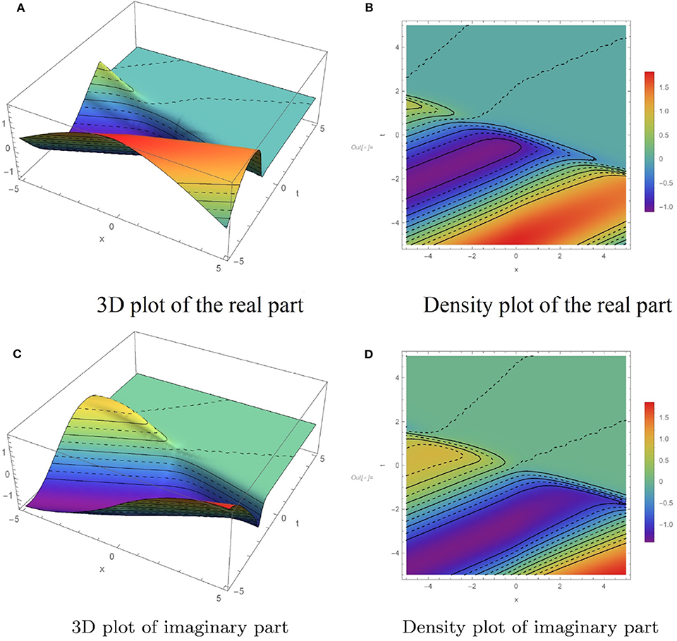
Figure 1. Dynamic behaviors of q₁(x, t) for a = 0.2, b = −0.5, c = 0.5, λ₁ = 3, λ₂ = 3, α = 0.97. (A) 3D plot of the real part. (B) Density plot of the real part. (C) 3D plot of imaginary part. (D) Density plot of imaginary part.

FIGURE 2

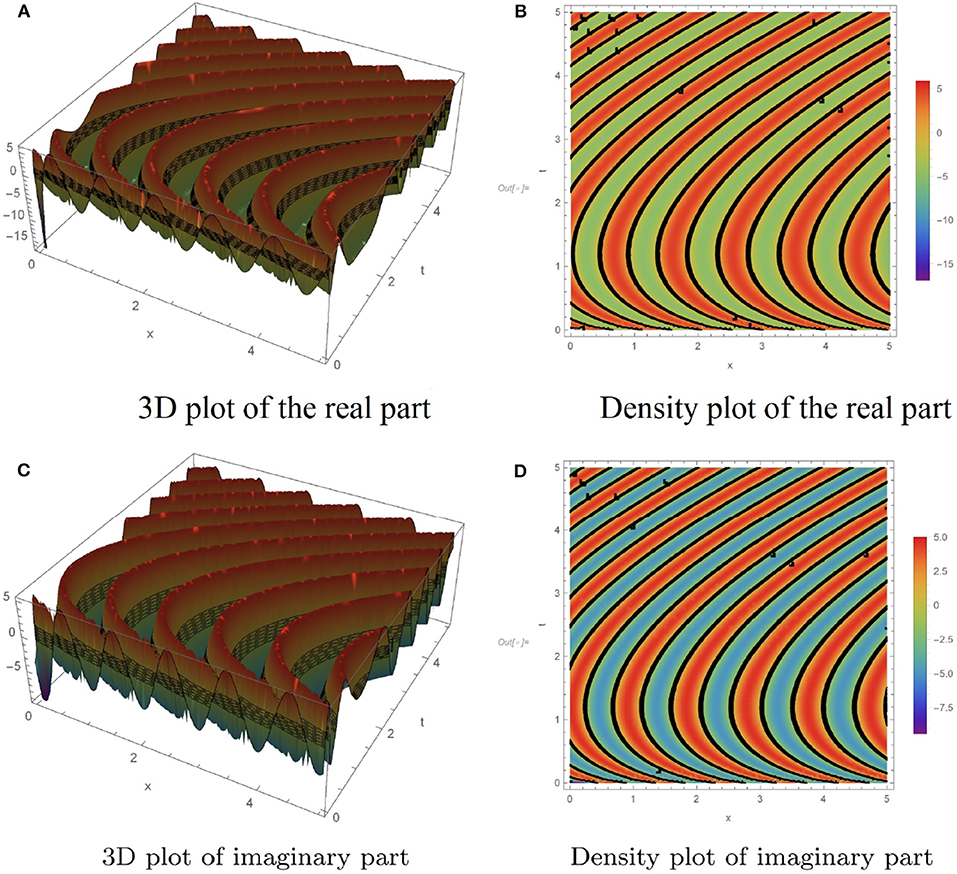
Figure 2. Dynamic behaviors of q₂(x, t) for a = −4, b = 2, c = 2, λ₁ = 0.1, λ₂ = 0.1, α = 0.95. (A) 3D plot of the real part. (B) Density plot of the real part. (C) 3D plot of imaginary part. (D) Density plot of imaginary part.

FIGURE 3

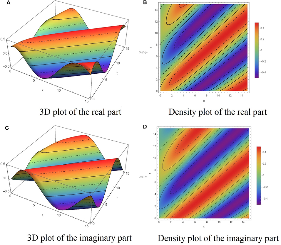
Figure 3. Dynamic behaviors of q₃(x, t) for a = 1, b = −3, c = 0.5, λ₁ = 1, λ₂ = 4, α = 0.9. (A) 3D plot of the real part. (B) Density plot of the real part. (C) 3D plot of the imaginary part. (D) Density plot of the imaginary part.

FIGURE 4

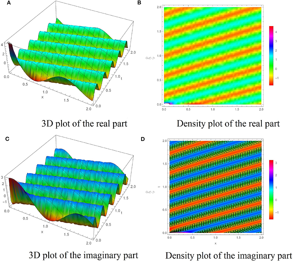
Figure 4. Dynamic behaviors of q₄(x, t) for a = 1.5, b = −2.5, c = 1, λ₁ = 7, λ₂ = 2, α = 0.9. (A) 3D plot of the real part. (B) Density plot of the real part. (C) 3D plot of the imaginary part. (D) Density plot of the imaginary part.

FIGURE 5

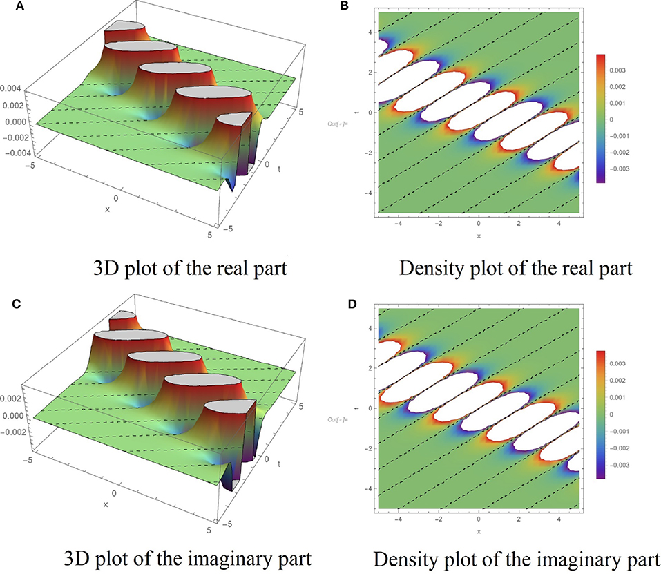
Figure 5. Dynamic behaviors of q₅(x, t) for a = 0.2, b = −2, c = 0.5, λ₁ = 2, λ₂ = 2, α = 0.99. (A) 3D plot of the real part. (B) Density plot of the real part. (C) 3D plot of the imaginary part. (D) Density plot of the imaginary part.

FIGURE 6

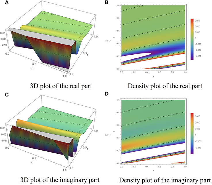
Figure 6. Dynamic behaviors of q₆(x, t) for a = 1.5, b = −5, c = 65, λ₁ = 0.3, λ₂ = 0.7, α = 0.9. (A) 3D plot of the real part. (B) Density plot of the real part. (C) 3D plot of the imaginary part. (D) Density plot of the imaginary part.

FIGURE 7

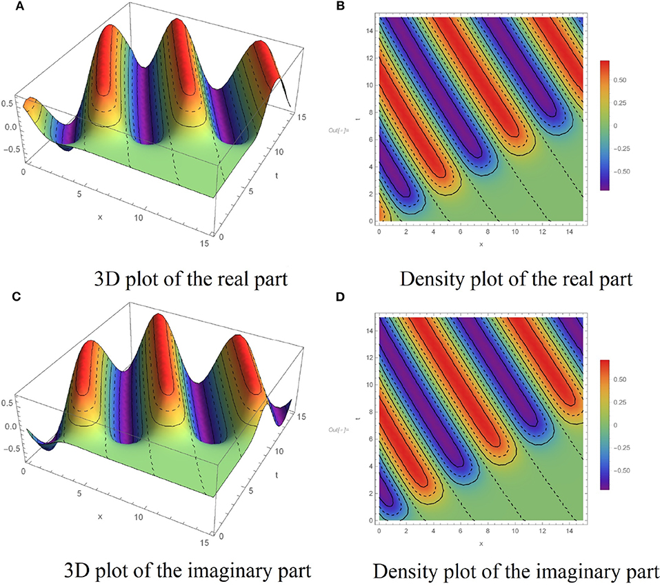
Figure 7. Dynamic behaviors of q₇(x, t) for a = −2, b = 3, c = 3.5, λ₁ = 2, λ₂ = 0.5, α = 0.95. (A) 3D plot of the real part. (B) Density plot of the real part. (C) 3D plot of the imaginary part. (D) Density plot of the imaginary part.

5. Conclusions

Partial differential equation is a powerful and effective tool for modeling non-linear systems. Finding the exact solution to such equations is one of the most challenging problems in mathematics. There is also no specific way of solving many of these equations. In these cases, we must resort to the approximate analytical methods due to the limitations of exact solver methods. According to what stated above, new approaches to solving PDE equations are of great importance and application. The main objective of this paper is to employ a well-known technique called GERFM to solve the perturbed Gerdjikov-Ivanov equation with the comfortable derivative. One of the outstanding features of the model considered in this article is the use of the definition of the comfortable derivative in the structure of the model. This definition is one of the most interesting definitions for a derivative that has many ideal features for a derivative. Applying this definition to the model will provide us with many advantages compared to the standard derivative. One of the advantages of the method used in this article is the determination of various categories of solutions during the method. Several numerical simulations are presented to gain a better understanding of the properties of the acquired solutions. By comparing the obtained results with the results of the present papers, it can be seen that the obtained results are not reported in any of the previous literature. It is worth mentioning that GERFM is capable of reducing the volume of needed computational compared to some other analytical method. The straightforward application is another advantage of the technique compared to other known techniques. This method can also be utilized to solve many other similar problems.

Data Availability Statement

The raw data supporting the conclusions of this article will be made available by the authors, without undue reservation, to any qualified researcher.

Author Contributions

All authors listed have made a substantial, direct and intellectual contribution to the work, and approved it for publication.

Conflict of Interest

The authors declare that the research was conducted in the absence of any commercial or financial relationships that could be construed as a potential conflict of interest.

References

1. Wazwaz AM. Partial Differential Equations and Solitary Waves Theory. Berlin; Heidelberg: Springer Berlin Heidelberg (2009).

Google Scholar

2. Arshad M, Seadawy AR, Lu D. Modulation stability and dispersive optical soliton solutions of higher order nonlinear Schrödinger equation and its applications in mono-mode optical fibers. Superlatt. Microstruct. (2018) 113:419–29. doi: 10.1016/j.spmi.2017.11.022

CrossRef Full Text | Google Scholar

3. Hosseini K, Samadani F, Kumar D, Faridi M. New optical solitons of cubic-quartic nonlinear Schrödinger equation. Optik. (2018) 157:1101–5. doi: 10.1016/j.ijleo.2017.11.124

CrossRef Full Text | Google Scholar

4. González-Gaxiola O, Franco P, Bernal-Jaquez R. Solution of the nonlinear Schrödinger equation with defocusing strength nonlinearities through the Laplace-Adomian decomposition method. Int J Appl Comput Math. (2017) 3:3723–43. doi: 10.1007/s40819-017-0325-5

CrossRef Full Text | Google Scholar

5. Arshed S, Biswas A, Abdelaty M, Zhou Q, Moshokoa SP, Belic M. Optical soliton perturbation for Gerdjikov-Ivanov equation via two analytical techniques. Chin J Phys. (2018) 56:2879–86. doi: 10.1016/j.cjph.2018.09.023

CrossRef Full Text | Google Scholar

6. Biswas A, Alqahtani RT. Chirp-free bright optical solitons for perturbed Gerdjikov-Ivanov equation by semi-inverse variational principle. Optik. (2017) 147:72–6. doi: 10.1016/j.ijleo.2017.08.019

CrossRef Full Text | Google Scholar

7. Yaşar E, Yıldırım Y, Yaşar E. New optical solitons of space-time conformable fractional perturbed Gerdjikov-Ivanov equation by sine-Gordon equation method. Results Phys. (2018) 9:1666–72. doi: 10.1016/j.rinp.2018.04.058

CrossRef Full Text | Google Scholar

8. Biswas A, Ekici M, Sonmezoglu A, Majid FB, Triki H, Zhou Q, et al. Optical soliton perturbation for Gerdjikov-Ivanov equation by extended trial equation method. Optik. (2018) 158:747–52. doi: 10.1016/j.ijleo.2017.12.191

CrossRef Full Text | Google Scholar

9. Arshed S. Two reliable techniques for the soliton solutions of perturbed Gerdjikov-Ivanov equation. Optik. (2018) 164:93–9. doi: 10.1016/j.ijleo.2018.02.119

CrossRef Full Text | Google Scholar

10. Kaur L, Wazwaz AM. Optical solitons for perturbed Gerdjikov-Ivanov equation. Optik. (2018) 174:447–51. doi: 10.1016/j.ijleo.2018.08.072

CrossRef Full Text | Google Scholar

11. Hosseini K, Mirzazadeh M, Ilie M, Radmehr S. Dynamics of optical solitons in the perturbed Gerdjikov-Ivanov equation. Optik. (2020) 206:164350. doi: 10.1016/j.ijleo.2020.164350

CrossRef Full Text | Google Scholar

12. Khalil R, Horani MA, Yousef A, Sababheh M. A new definition of fractional derivative. J Comput Appl Math. (2014) 264:65–70. doi: 10.1016/j.cam.2014.01.002

CrossRef Full Text | Google Scholar

13. Eslami M, Rezazadeh H. The first integral method for Wu-Zhang system with conformable time-fractional derivative. Calcolo. (2015) 53:475–85. doi: 10.1007/s10092-015-0158-8

CrossRef Full Text | Google Scholar

14. Atangana A, Baleanu D, Alsaedi A. New properties of conformable derivative. Open Math. (2015) 13:81. doi: 10.1515/math-2015-0081

CrossRef Full Text | Google Scholar

15. Çenesiz Y, Baleanu D, Kurt A, Tasbozan O. New exact solutions of Burgers' type equations with conformable derivative. Waves Random Complex Med. (2016) 27:103–16. doi: 10.1080/17455030.2016.1205237

CrossRef Full Text | Google Scholar

16. Anastassiou G. A. editor. “Fractional conformable approximation of Csiszar's f-divergence,” in Intelligent Analysis: Fractional Inequalities and Approximations Expanded. Cham: Springer International Publishing (2020). p. 463–480. doi: 10.1007/978-3-030-38636-8_25

CrossRef Full Text | Google Scholar

17. Harir A, Melliani S, Chadli LS. Fuzzy generalized conformable fractional derivative. Adv Fuzzy Syst. (2020) 2020:1–7. doi: 10.1155/2020/1954975

CrossRef Full Text | Google Scholar

18. Zafar A, Seadawy AR. The conformable space-time fractional mKdV equations and their exact solutions. J King Saud Univ Sci. (2019) 31:1478–84. doi: 10.1016/j.jksus.2019.09.003

CrossRef Full Text | Google Scholar

19. Zafar A, Raheel M, Bekir A. Exploring the dark and singular soliton solutions of Biswas-Arshed model with full nonlinear form. Optik. (2020) 204:164133. doi: 10.1016/j.ijleo.2019.164133

CrossRef Full Text | Google Scholar

20. Zafar A, Rezazadeh H, Bekir A, Malik A. Exact solutions of (3+1)-dimensional fractional mKdV equations in conformable form via exp (−ϕ(τ)) expansion method. SN Appl Sci. (2019) 1:11. doi: 10.1007/s42452-019-1424-1

CrossRef Full Text | Google Scholar

21. Rezazadeh H, Vahidi J, Zafar A, Bekir A. The functional variable method to find new exact solutions of the nonlinear evolution equations with dual-power-law nonlinearity. Int J Nonlin Sci Numer Simul. (2019). doi: 10.1515/ijnsns-2019-0064. [Epub ahead of print].

CrossRef Full Text | Google Scholar

22. Zafar A. Rational exponential solutions of conformable space-time fractional equal-width equations. Nonlin Eng. (2019) 8:350–5. doi: 10.1515/nleng-2018-0076

CrossRef Full Text | Google Scholar

23. Ghanbari B, Inc M. A new generalized exponential rational function method to find exact special solutions for the resonance nonlinear Schrödinger equation. Eur Phys J Plus. (2018) 133:1. doi: 10.1140/epjp/i2018-11984-1

CrossRef Full Text | Google Scholar

24. Osman MS, Ghanbari B. New optical solitary wave solutions of Fokas-Lenells equation in presence of perturbation terms by a novel approach. Optik. (2018) 175:328–33. doi: 10.1016/j.ijleo.2018.08.007

CrossRef Full Text | Google Scholar

25. Ghanbari B, Baleanu D. A novel technique to construct exact solutions for nonlinear partial differential equations. Eur Phys J Plus. (2019) 134:506. doi: 10.1140/epjp/i2019-13037-9

CrossRef Full Text | Google Scholar

26. Ghanbari B, Baleanu D. New solutions of Gardner's equation using two analytical methods. Front Phys. (2019) 7:202. doi: 10.3389/fphy.2019.00202

CrossRef Full Text | Google Scholar

27. Srivastava HM, Günerhan H, Ghanbari B. Exact traveling wave solutions for resonance nonlinear Schrödinger equation with intermodal dispersions and the Kerr law nonlinearity. Math Methods Appl Sci. (2019) 42:7210–21. doi: 10.1002/mma.5827

CrossRef Full Text | Google Scholar

Keywords: PDEs, generalized exponential rational function method, non-linear Schrödinger equation, exact solutions, the perturbed Gerdjikov-Ivanov equation

Citation: Ghanbari B and Baleanu D (2020) New Optical Solutions of the Fractional Gerdjikov-Ivanov Equation With Conformable Derivative. Front. Phys. 8:167. doi: 10.3389/fphy.2020.00167

Received: 22 February 2020; Accepted: 22 April 2020;
Published: 15 May 2020.

Edited by:

Jordan Yankov Hristov, University of Chemical Technology and Metallurgy, Bulgaria

Reviewed by:

Hernando Quevedo, National Autonomous University of Mexico, Mexico
Asim Zafar, COMSATS University Islamabad, Pakistan
Necati Özdemir, Balıkesir University, Turkey

Copyright © 2020 Ghanbari and Baleanu. This is an open-access article distributed under the terms of the Creative Commons Attribution License (CC BY). The use, distribution or reproduction in other forums is permitted, provided the original author(s) and the copyright owner(s) are credited and that the original publication in this journal is cited, in accordance with accepted academic practice. No use, distribution or reproduction is permitted which does not comply with these terms.

*Correspondence: Behzad Ghanbari, b.ghanbary@yahoo.com

ORIGINAL RESEARCH article

New Optical Solutions of the Fractional Gerdjikov-Ivanov Equation With Conformable Derivative

1. Introduction

2. Mathematical Preliminaries and Backgrounds

2.1. Analysis of GERFM

2.2. The Conformable Derivative

3. Mathematical Analysis

4. Numerical Simulations

5. Conclusions

Data Availability Statement

Author Contributions

Conflict of Interest

References

This article is part of the Research Topic

People also looked at