Potentialities of the combined use of underwater fluorescence imagery and photogrammetry for the detection of fine-scale changes in marine bioconstructors

1 Introduction

Bioconstructor species, such as corals and gorgonians, create reefs that sustain an extremely high biodiversity, provide key ecosystem services to the global economy, and influence important ecological processes (Cerrano et al., 2010; De La Torriente et al., 2020). Habitat-forming corals are endangered by multiple large-scale and local pressures, facing both natural disturbances and anthropogenic stressors (Sobha et al., 2023). Global warming and invasive predators threaten coral cover and reef complexity, affecting their three-dimensional (3D) structure (Righi et al., 2020; Chimienti et al., 2021). Moreover, human-mediated impacts, such as marine pollution, overfishing and physical damage caused by boat anchoring, constitute critical drivers of coral decline (Forrester et al., 2015; Forrester, 2020). These threats call for urgent actions and have resulted in international guidelines for the preservation of these habitats (Gómez-Gras et al., 2019).

Monitoring the health status of endangered bioconstructors to detect and quantify the impact of local and global stressors demands a high degree of accuracy and fine-scale resolution. Detecting changes in the structural complexity of coral reefs and single colonies is critical to reversing the current downward trends of these ecosystems, fostering protection and restoration purposes. Classical underwater surveys rely on in-situ observations and measures performed by specialized certified divers, provided with a self-contained underwater breathing apparatus (SCUBA). These operations have to cope with several safety and logistic constraints, like the danger of some habitats (for instance caves) and require a considerable observation time if high-quality data are needed. Additionally, these procedures often imply the manipulation of corals, and the destructive sampling of colonies for further laboratory analyses and measures (including surface area and volume) (Million et al., 2021). In-situ non-invasive biometric techniques are often strictly related to the morphology of the colony and can be applied only on branching or massive species, while visual estimates performed by SCUBA divers could be accurate at reef scale but may not detect finer scale structures and changes. Furthermore, they are affected by inter-observer variability (Gutierrez-Heredia et al., 2016), and manual polyp counting could be hardly applied to massive coral colonies underwater.

Due to modern technological advances in computer vision, change-detection techniques for investigating the health of corals permit the analyses of live cover, counting species presence/absence and decay, and the assessment of benthic assemblages (Gutierrez-Heredia et al., 2016; Kersting et al., 2017; Kopecky et al., 2023). The photogrammetric approach allows non-intrusive measurements from digitalized 3D models of organisms, relying on an array of two-dimensional camera images taken from different points of view (Figueira et al., 2015). To reduce fundamental errors and obtain metrically accurate 3D models, external constraints to photogrammetric reconstruction are essential. Constraints can be positioned on the seabed (Rossi et al., 2020) or referred to as camera pose during image acquisition (Nocerino and Menna, 2023). During the last few years, this technique has been largely employed to map marine habitats on a large scale and study benthic assemblages (Marre et al., 2019). Close-range photogrammetry has been successfully utilized to obtain measures of coral colony dimensions, surface area and 3D complexity (Courtney et al., 2007; Burns et al., 2015; Lavy et al., 2015; Guo et al., 2016; Gutierrez-Heredia et al., 2016; Ferrari et al., 2017) and is widely adopted in marine investigations from habitat scale (Bongaerts et al., 2021) to individual phenotyping (Million et al., 2021; Kopecky et al., 2023). These tools provide accurate measurements of lengths, areas, and volumes that are difficult or even impossible to get in situ with traditional methods (Bayley et al., 2019). Despite these benefits, several aspects of underwater photogrammetry need further studies. Underwater 3D reconstructions have revealed significant environmental constraints related to the noise produced by water turbidity, non-uniform lighting, and image quality and resolution, which could reduce image accuracy and hinder the alignment stage by introducing errors (Lavy et al., 2015; Gutierrez-Heredia et al., 2016). Underwater images always show color cast, e.g., green-bluish color, which is caused by different attenuation ratios of red, green, and blue lights. Also, the particles that are suspended underwater absorb most of the light energy and change the direction of light before the light reflected from underwater scenes reaches the camera, which leads to images having low contrast, blur, and haze (Oakley and Satherley, 1998). Thus, extracting valuable information from underwater scenes requires effective methods to correct color, improve clarity and address blurring and background scattering, which is the aim of image enhancement and restoration algorithms (Akkaynak and Treibitz, 2019; Wang et al., 2019).

Fluorescence analysis has been proposed in underwater applications to analyze coral reefs (Treibitz et al., 2015), since together with reflectance, it constitutes a recognized tool for the assessment of animal and plant vitality. The use of fluorescence analysis is recognized for plant monitoring in terrestrial applications, but due to increased technical complications, has not yet reached the same level of maturity in underwater applications. As a result, despite its potential for the change-detection of coral health conditions, this approach has been understudied and has not been implemented in field applications so far (Sasano et al., 2016; Ramesh et al., 2019). Limited attempts are documented, mainly including fluorescence analyses within wider spectroscopic techniques often requiring the use of multispectral imagers (Caldwell et al., 2017; Zweifler et al., 2017; Teague et al., 2022).

In the present study, the development, testing and validation of a novel and transferable multi-sensor measuring system were performed. The system is based on the integration of photogrammetry and fluorescence imagery. It will be suitable for being used by SCUBA divers at the local scale for detecting fine-scale changes in coral morphology or can be equipped onboard underwater remotely operated vehicles (UROVs) for wide areas mapping and monitoring. The application of UROVs for coral monitoring is largely unexplored as well. Its feasibility in the common scientific practice still needs to be validated to the traditional approach: early-stage attempts are provided by Price et al. (2019) to quantify the structural complexity of cold-water coral reef patches. The novelty of the present research lies in the integration of emerging techniques that can be applied to a wide range of 3D morphometric measurements, different habitats, and species, thus paving the way to innovative opportunities in ecological research and more effective results than traditional in-situ monitoring methods.

The system setup was developed and tested in the laboratory, validating multiple variables such as the influence of a reflex camera coupled with a commercial underwater housing, flying elevation, camera orientation and photo density, to achieve high values of accuracy and precision of the 3D reconstructions. These goals were vital to address a sub-centimetric resolution for measuring relevant biometric parameters (polyp counting, colony surface areas and volumes) and detect changes in coral health status at a fine scale and under natural lighting through autofluorescence analysis. In particular, the integration of photogrammetry and fluorescence imagery, which will be actual onboard of a ROV where the presented components will be combined, has the potential to provide a cost-effective, flexible, and easy-to-use approach to identify the health status of several zooxanthellate species. The main challenge consists in pursuing the implementation of the safeguard of coral ecosystems, intending to detect threats to biodiversity before significant adverse impacts occur.

2 Materials and methods

2.1 Coral sampling and experimental treatments

Photogrammetry and fluorescence imagery data capturing, image enhancement, and strategies for multi-temporal analyses were performed on live colonies of Cladocora caespitosa as a model. This endemic zooxanthellate coral is the most important reef-building species in the Mediterranean (Roveta et al., 2023), and it is included in the Red List of the International Union for the Conservation of Nature (IUCN) as an endangered species (Kersting et al., 2023; https://www.iucnredlist.org/species/133142/165739749). Coral fragments were retrieved at San Vito Lo Capo (38°10′N, 12°45′E, Trapani, Italy) in September 2021 at 15 m depth, among those naturally detached from the substrate after sea storms. Selected healthy corals (with colored polyps and with no signs of necrosis or bleaching) were maintained in aerated tanks and transported to the laboratory at the University of Modena and Reggio Emilia within a few days. There, corals were transferred in a 300 L tank of a 950 L recirculating seawater aquarium system with controlled conditions: temperature 17 ± 2°C maintained with a heater exchanger (TEKO TK500), salinity 36-38, photoperiod 12 h light/12 h dark using a LED lamp (Easy LED Aquatlantis). They were fed ad libitum with nauplii of the crustacean Artemia franciscana (Rodolfo-Metalpa et al., 2008) and left to acclimate for two weeks before starting the experiments. Three coral fragments were selected to evaluate the effectiveness of the setup of the system, with particular concern to the equipment installation and use, and the procedures for data processing. They were arbitrarily labeled C6, C10 and C20 and displayed different morphotypes (Figures 1A–C): C6 was an entire mounding colony, while C10 and C20 were artifacts simulating small colonies, obtained by mounting coral fragments on a small brick with a bicomponent coral glue (Coral Gum Instant, Tunze). The study is exempt from ethics approval per the local legislation and was performed following the requirements of the University of Modena and Reggio Emilia.

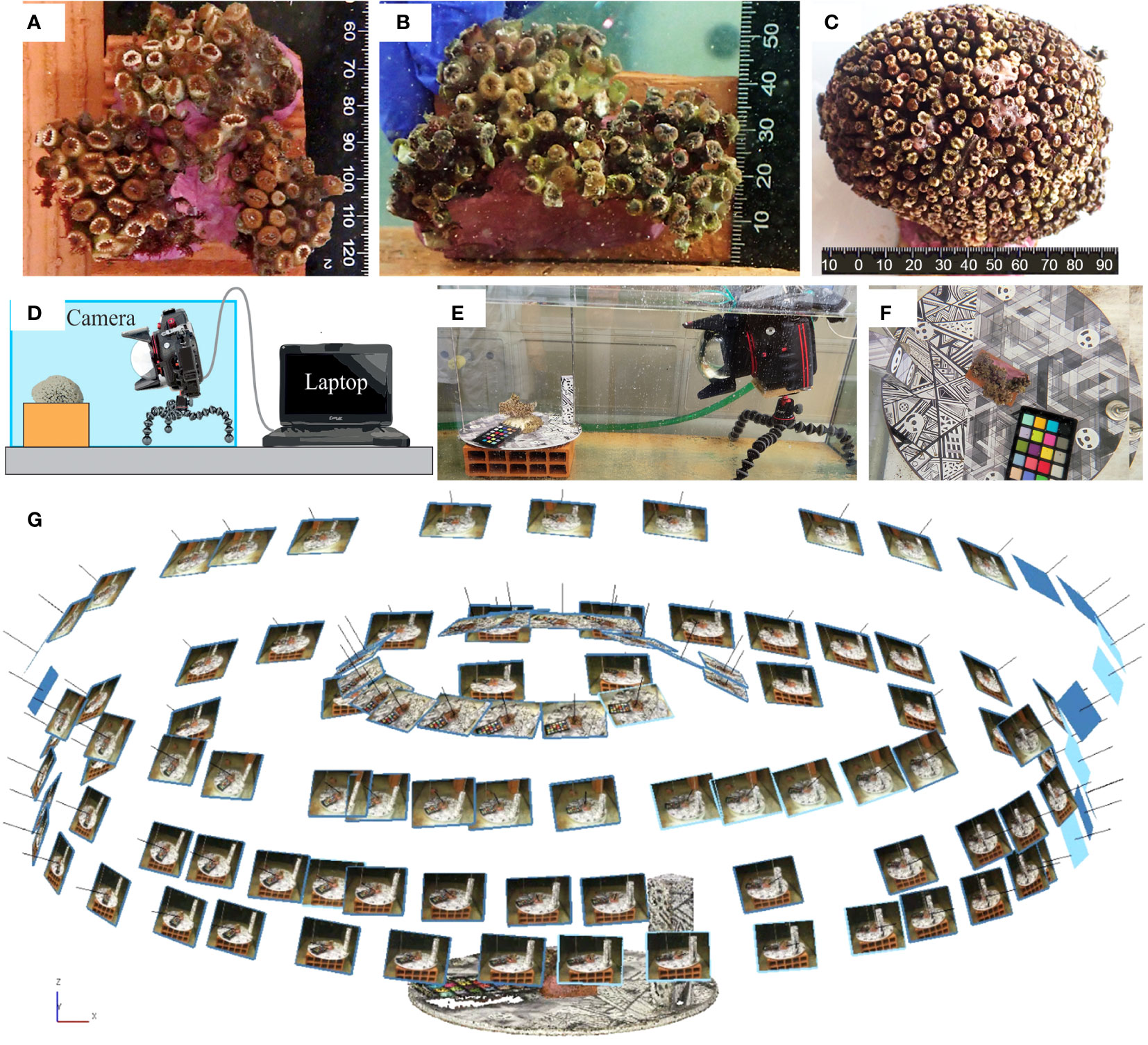
Figure 1 The investigated samples of Cladocora caespitosa: (A) C10; (B) C20; (C) C6. (D, E) A schematic representation and a real picture of the setup for the camera and the sample as adopted during the photogrammetric data collection. (F) Focus on the designed reference plate containing targets for Ground Control Points (GCPs) and geometric textures to help Tie Points (TPs) identification. (G) An example of the geometric scheme adopted for collecting the photogrammetric dataset.

To verify the ability of the investigated methods to identify alterations in the state of health of marine bioconstructors, the three coral fragments were analyzed by repeating the same analyses before and after the application of specific stresses or the occurrence of natural degradation. The state of health of single corallites was assessed through analyses of coral 2D and 3D biometry and/or fluorescence before and after stressful events (i.e. experimental treatments). Measures and experimental treatments were performed on each coral in different moments (even weeks apart) identified as “Epochs”. A first baseline acquisition, before receiving the treatments, was carried out and will be identified through the manuscript as Epochs 0 and 1* depending on the observed coral fragment, the sensor used and the time difference among data acquisition events. In Epochs 1, 2, and 3, the corals changed their state of health due to natural degradation (i.e., C6, which did not receive stresses) or induced mechanical stresses (i.e., C10 and C20). For the fluorescence tests, the reference epoch was always the first epoch when fluorescence observations were carried out and refer to the unstressed and unperturbed condition; it was identified as Epoch 0 for the C20 sample and as Epoch 1* for the C10 sample (this epoch is the fluorescence baseline because we waited 3 months after the first anchor damage induced on the sample, thus we can consider the sample as unstressed). For a better comprehension of Epochs and related data collected, please refer to Table 1 which describes the structure of experimental tests, with details on the type of stresses imposed on the colony samples. The temporal dimension is reported as the time interval, expressed in months, between the specific epoch and Epoch 0.

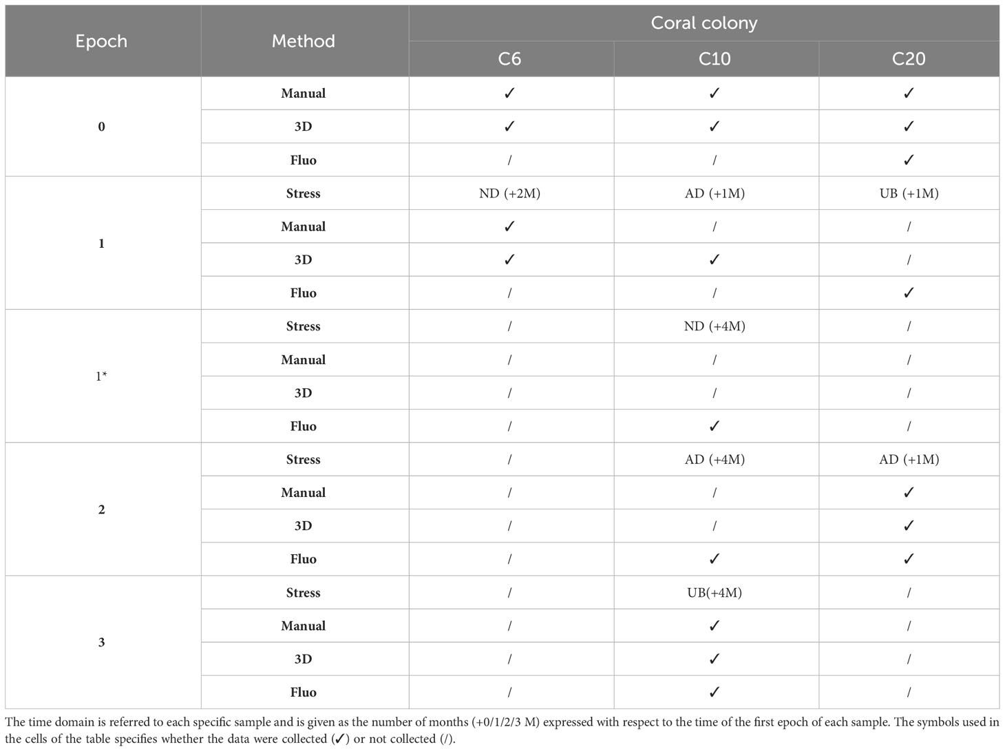
Table 1 List of the collected datasets with reference to the time domain (different epochs), the adopted methods and the experimental stresses applied to the investigated specimens (AD = Anchor Damage; UB = Ultrasonic Bath; ND = Natural Degradation).

Stressful events consisted of mechanical stresses provided by the impact with an anchor and the dipping of part of the colony in an ultrasonic bath. Each of the C. caespitosa fragments (i.e., C10 or C20) was placed in a cylindrical plastic container (30 cm wide and 32 cm high), and the anchor (1.5 kg) was dipped down until the flukes entered the water in axis with the target point of the coral. Then, the anchor was dropped from about 10 cm by gravity. Coral ultrasonication (which destroys the soft tissues and simulates coral necrosis) was performed in a stainless-steel ultrasound bath (Elma Inc., Model D-7700 Singen/Htw.; power 230 W) with a frequency of 35 kHz. The coral was partially immersed in the bath in such a way that only a known portion of its surface was exposed to ultrasounds for 10-15 seconds. The temperature and salinity of the water in the cylindrical container and ultrasound bath were the same as in the aquarium system.

2.2 Colony morphology and biometry and polyp health status

First, coral morphology was described based on planar (2D) underwater photos next to a ruler, using an underwater digital camera (Olympus Tough TG-6) (see for example Roveta et al., 2023). The positioning of the corals and the ruler on the same plane requires special attention, to reduce perspective distortions caused by different distances between the two objects and the camera lens. These could not be always avoided because of the 3D geometry of corals, which cannot be aligned at every point at the same time with a two-dimensional ruler. Moreover, the margins of the images can be often distorted by the “fisheye effect”, due to the wide-angle lens mounted on most of the underwater compact cameras commercially available. Fragments of C. caespitosa were positioned on a plane and photographed three times to account for frames showing length, height, and width. In the case of C6, which was considerably larger than C10 and C20, it was moved briefly in the air to obtain photographs from multiple views to count single corallites. To avoid repetitions during the manual counting of corallites, this mounding colony was divided into sectors by passing a thread among corallites before taking the photos. Then, each sector was analyzed separately using a graphic editor to mark corallites with different colors while counting, based on their health state: healthy (polyps with brown turgid oral disc), bleached (dead white corallites or completely covered by algae), and partially bleached (if the edge of the calyx was white but the center was still brownish) (Antoniadou et al., 2023). All the photos were processed using the image analysis software ImageJ (Ferreira and Rasband, 2012). Once imported into the software, each image was zoomed on the metric reference to scale it. Similar analyses were also performed on generated 3D models; the “point list picking tool” available in the open-source software Cloud Compare v. 2.11 was used. While translating, rotating, and zooming the model, the user can select and label points of interest, the software counts them automatically. The observation of macro details from different perspectives allowed the detection of minimal changes in the colony surface due to the presence (or absence) of corallites. The points selected were grouped in categories based on the health state of corallites and displayed separately on the 3D model.

Coral fragments had roughly elliptical shapes and the main size descriptors collected were maximum and minimum diameters (D1, D2, respectively; Kersting and Linares, 2012) and height (H), since they show positive correlations between each other (Kersting and Linares, 2012). Colony morphology was described using the Is-index to derive coral sphericity (Is-index = maximal height of the colony / maximal diameter of the colony; Kružić and Benković, 2008). In the case of C. caespitosa, a scalene ellipsoid could most accurately approximate the surface area of coral colonies (Ac), measuring widths (i.e., maximum, and minimum diameters) and height from two perpendicular images of the coral. Given that the base of the colony is flat, the area should be considered as 75% of the scalene ellipsoid and was calculated using the formula:

where p ~ 1.6075 based on Knud Thomsen’s formula for the surface area of a general ellipsoid.

2.3 Image acquisition for photogrammetry

The coral specimens were examined under laboratory conditions. Coral fragments were fixed over small supports (rock, seashell, or small pieces of tile) to guarantee the stability of the sample in the tank and during the acquisition of the images. Underwater imaging was performed using a Canon 2000D reflex camera and an 18-55 mm EFS lens, coupled with an underwater housing (Easy Dive LEO3) equipped with a dome port (Figures 1D, E). The dome port allows for a reduction of image distortion and the achievement of more accurate results (Menna et al., 2016; Menna et al., 2017). The camera resolution was 24.1 Mpixels. The acquisition distance was about 50 cm and constant during the test resulting in images with a resolution of 0.05: 0.06 mm. These choices allowed the detection of numerous details and the generation of high-resolution reconstructions (resolution of about 0.1 mm). Images were acquired with a 35mm focal length, in automatic and autofocus mode, and with an exposure time of 1/50. The f-number was about 8.75 for all datasets and the depthof field was about 3.5 cm. More information about data acquisition can be found in Table 2. Also, according to Nocerino et al. (2022), the image stabilization system was switched off to increase image precision. Photogrammetric processing requires external references to reduce distortion effects due to the water medium and obtain a scaled geometry and an accurate 3D reconstruction (Istenič et al., 2020; Rossi et al., 2020). A set of 12 targets (Agisoft Metashape circular targets, 12-bit resolution) with known coordinates was used to constrain the photogrammetric reconstruction. The 12 points were defined as follows: six points are the vertexes of a regular shape, a hexagon, and they were printed on a planar surface (later referred to as “plate”) whereas further six targets were added to a 10 cm height parallelepiped, orthogonal to the planar surface and providing a vertical constraint as well. In this way, the coordinates, and the relative distances, were obtained within a conventional coordinate system, as created within a common CAD environment. Each of the investigated coral fragments was positioned on the plate with the targets wrapping the fragment (Figure 1F). A rigid unambiguous placement of the specimen over the plate was not designed, thus each 3D reconstruction was in its local reference system; a co-registration was required to perform temporal comparisons. The surface of the plate also displayed a heavily textured design consisting of geometric shapes in a grey color scale to facilitate image matching (in Gutierrez-Heredia et al., 2016 a similar solution was adopted), as displayed in Figure 1F. The camera was mounted over a small tripod (JOBY Kit Gorillapod 5K) and maintained stable through lead weights; the reference plate was manually rotated during image collection. Four sets of images were captured performing full circles around the sample with viewing angles ranging from sub-horizontal to sub-nadiral (approximately 20°, 45°, 60°, 80° - Figure 1G), ensuring a strong redundancy, geometry constraint, accurate results, and reducing occlusion areas (Gutierrez-Heredia et al., 2016; Lange and Perry, 2020). About 30 images were acquired for each set and no zooming images were included, for a total of 120 images per sample per test.

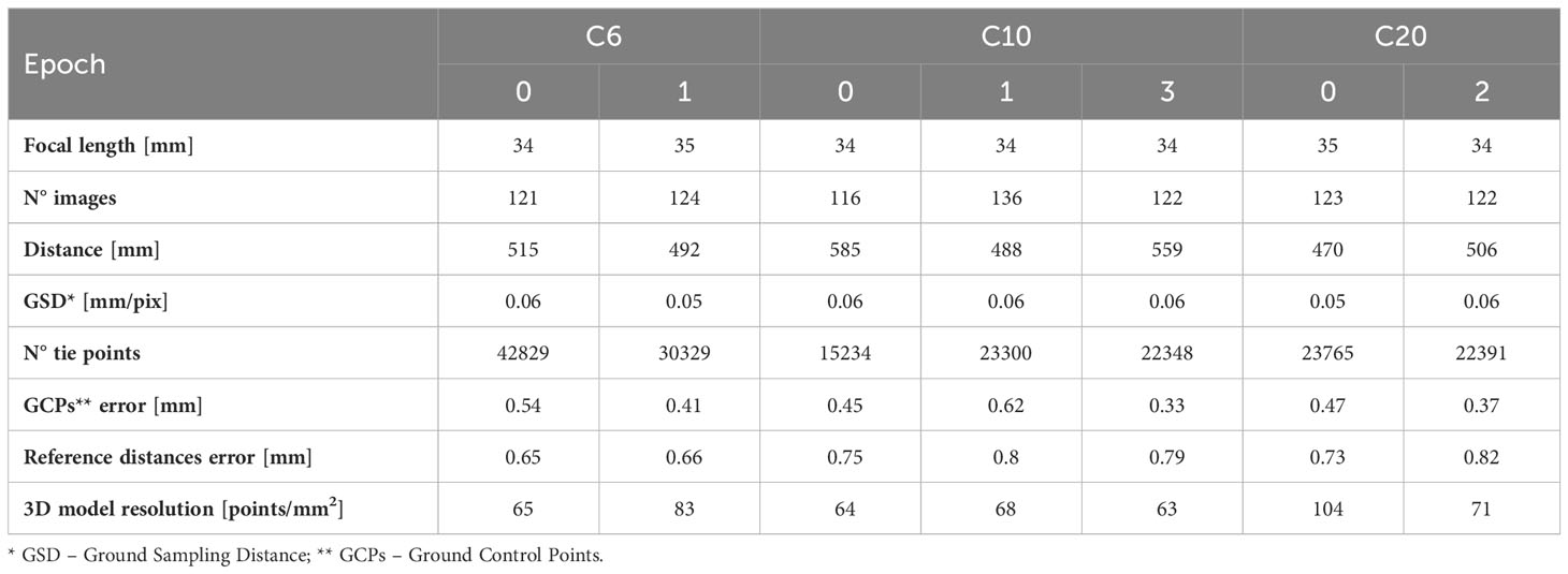
Table 2 List of the main parameters regarding the photogrammetric processing along with the properties of the final 3D model.

Image sets were then processed using the photogrammetric software Agisoft Metashape (v. 1.7), which is largely used for underwater applications (Gutierrez-Heredia et al., 2016; Bayley and Mogg, 2020; Burns et al., 2020; Ventura et al., 2021). The software uses automatic feature recognition to register images that serve as tie points (TPs) for the collected dataset and allow the generation of a sparse point cloud, obtain camera poses and orientation, and estimate internal camera parameters in an arbitrary reference system. The overall datasets were analyzed before starting the processing to delete bad-quality images. A proper function is implemented in Agisoft Metashape, but in this case, the authors found a manual check of images more effective for deleting bad-quality images: bad focused, bad centered, or with blurry effects. Images were automatically masked to focus the search of tie points only on the coral fragment and the reference plate, avoiding the background and the tank. The relative orientation of images was performed with the highest option in terms of the accuracy of the results. Noisy tie points were manually deleted and tie points with high reprojection errors were automatically selected and removed before optimizing the relative orientation. Authors found that values of reprojection errors depended on the acquired dataset, and they varied even if similar acquisition conditions were guaranteed. In this study, authors preferred to delete a constant percentage of tie points (20-30% of the total). This is a common practice rather than setting a fixed threshold that is hard to define. The center of the targets was automatically identified, and then positions were manually checked to minimize high reprojection errors on ground control points (larger than 3÷4 pixels). The external metric references were then added to the project by using as input both the targets’ coordinates and their relative distances. Being created mathematically, these references are in theory exact. To consider errors during the printing process and the physical construction of the rotating support, a precautionary accuracy of 0.5mm for all the external references was considered. Optimization of relative orientation was run iteratively, and results were obtained in the local reference system given by the targets. The calculated outputs were then used for the dense point cloud computation. The original image’s resolution was halved, and an aggressive depth filter was used. Outliers in the dense point cloud and points with weak statistics were removed. The remaining points form the dense point cloud, the final output of the photogrammetric processing to be used for mesh production, multi-temporal analyses, and quantitative assessment of biometric parameters. A full 3D textured mesh was built with a number of faces twice the original vertexes; for texture generation, a subsample of the original dataset was used. Dense point cloud was exported in.txt format maintaining the information about points’ position, colors and normal (columns list the following variables: X, Y, Z, R, G, B, Nx, Ny, Nz). Textured meshes were exported in.obj format, coupled with.jpeg format for the texture and were used in this work for coral visualization and as a support for morphology and analyses of biometry.

2.4 Image quality improvement

In the present research activity, the images were carried out in laboratory conditions where water turbidity was under control and the distance between the camera and the marine species was extremely limited (about 50cm). Due to these logistic constraints, raw images were originally acceptable and did not require the implementation of a full restoration process to improve the quality. The authors applied a traditional color correction method, white balancing (WB), to modify the color and saturation. WB falls within the image enhancement methods based on a single-color model (Wang et al., 2019). To this end, a color checker was placed in the tank, close enough to the coral fragment to be included within all photos, during image collection. In this way, raw images were processed first to slightly improve the radiometric quality before the photogrammetric process in Section 2.3. Image restoration strategies (Wang et al., 2019) would be mandatory when dealing with open water-collected datasets to improve the quality of underwater images before using them for 3D model production and biometric analyses.

2.5 Image acquisition for fluorescence

The analysis of the fluorescence generated by the corals was performed by illuminating them with a UV LED source (model UltraFire H-B3, emission peak at 470 nm) and acquiring the images using a Canon 2000D camera (the same used for the photogrammetric analysis, Figure 2B). A schematic representation of the setup used is shown in Figure 2A.

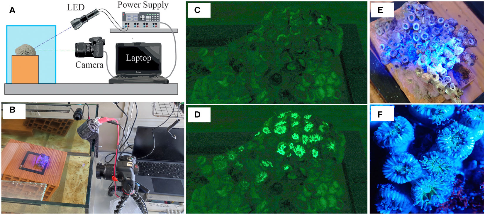
Figure 2 (A) Schematic representation of the setup used for fluorescence analysis. The sample is illuminated using the UV LED source and the images are acquired employing the camera. The UV LED source is powered by the power supply. The switching on of the UV LED source, as well as the acquisition of the images, are controlled by a software application written in LabVIEW. (B) Picture of the real measuring system. (C) RGB image of the sample captured by the Canon 2000D camera when the LED source was off (the dark phase). (D) RGB image of the sample captured by the Canon 2000D camera when the LED source was on (the excitation phase). (E) Picture of the sample obtained during the excitation phase using a second camera positioned approximately orthogonally to the free surface of the water. (F) Zoom in of the previous picture for highlighting the most illuminated area during the excitation phase.

Fluorescence intensity linearly depends on the quantum yield of the fluorophore and is a monotonic increasing function of the fluorophore concentration and the optical power absorbed by the fluorophores (Lakowicz, 1992; Lakowicz, 2006). Therefore, if the fluorophores in the sample are not too concentrated and the irradiance of the excitation source is low enough not to generate photobleaching, the fluorescence intensity grows as the concentration of the fluorophores and the irradiance generated by the excitation source increases. To extract the concentration of fluorophore in the coral fragments from the images, it is necessary to compensate for the contribution of all the other quantities of influence affecting the image provided by the camera. The coral autofluorescence we analyzed results in an emission peak in the green spectral region. Thus, we considered the green channel of the RGB image provided by the camera (Alieva et al., 2008). The radiant energy collected by each pixel of the camera during the exposure time is given not only by the radiant power of the fluorescence generated by the coral under test but also by the radiant power of the reflection on the coral surface of the radiation generated by the LED source and by ambient lighting. In this regard, it is important to consider that LED sources typically have a band of tens of nanometers and that, therefore, even if the peak wavelength of the source used for excitation is outside the spectral region of the emission of the fluorophore, the tail of the source used for excitation may partially overlap with the fluorescence emission spectral region Figures 2E, F. Considering that the fluorescence intensity is generally well lower than the excitation intensity, it is important to avoid the excitation radiation containing spectral components in the spectral region of the fluorescence emission.

To minimize the error due to the reflection of the beam generated by the LED source, the source was filtered with a microscopy filter centered on C. caespitosa excitation peak [excitation filter, model FXF001, by Thorlabs - Transmission Wavelength (430, 470) nm]. Similarly, the camera lens was filtered using a filter centered on the coral emission peak [emission filter, model FXF002, by Thorlabs - Transmission Wavelength (515, 535) nm]. In this way, the excitation and emission of fluorescence occur in two different and separate spectral regions thus, it is possible to distinguish them. The joint use of these filters produces an attenuation of the out-of-band radiation nominally higher than 10⁶. Therefore, less than ${10}^{-6}$ of the excitation radiation reflected from the sample towards the camera reaches its detector pixels. Furthermore, the LED source was positioned in such a way as to prevent the specular reflection of its beam from entering the camera’s aperture stop. Then, the supply voltage of the LED source was set to avoid photobleaching. The camera lens filter (emission filter) not only minimizes the fraction of the radiant power generated by the LED source that reaches the camera pixels but also reduces the radiant power that reaches the pixels due to the reflection of ambient lighting. Theoretically, of all the ambient light reflected by the sample, only the spectral component in the emission filter’s transmission band can reach the camera pixels.

Although the presence of the filter reduces the contribution of ambient lighting, the radiant power resulting from the transmission of the ambient lighting through the emission filter is in general not negligible compared to the radiant power resulting from fluorescence. Therefore, in the presence of ambient lighting, the contribution of the latter is such that, if not compensated, it can lead to significant errors in the estimate of the intensity of the fluorescence signal. The development of a measurement method capable of compensating for the radiant power from the ambient lighting was required. We, therefore, acquired a series of images in rapid succession in two phases. In the first phase, called the dark phase, $N_{img}=3$ images were acquired keeping the LED source off (Figure 2C). Then, in the second phase called the excitation phase, the LED source was turned on, and $N_{img}=3$ more images were acquired in rapid succession (Figure 2D). The intensity of the images acquired during the dark phase depends on the radiant power due to the ambient lighting only. Given that, thanks to the use of filters, the contribution of the UV LED source in the green image is negligible, the intensity of the images acquired during the excitation phase depends on the radiant power due to both the fluorescence and the ambient lighting, but not on the reflection of the excitation light. Hence, under the assumption that the ambient illumination remained constant between the dark and excitation phases and that the sample did not move, the pixel-by-pixel subtraction of the dark image from the excitation image gives, theoretically, the intensity due to fluorescence only.

The acquisition of $N_{img}$ images for each of the two phases allowed us to verify the reasonableness of the assumption of unchanged ambient lighting. From each of the two sets of images acquired at time t, we obtained the average green images $\underset{\_}{I_{dark}}(t)$ and $\underset{\_}{I_{excitation}}(t)$ through pixel-by-pixel averaging. Thus, we calculated the fluorescence image, $\underset{\_}{I_{fluorescence}}(t)$, as the difference between the average excitation image and the average dark image:

For this compensation to be effective, it is also necessary for the camera settings to remain unchanged, and the non-linear functions implemented by the camera being disabled (e.g. the Gamma correction).

Once the two sets of images were acquired, the system went into an idle state by switching off the LED source for 60 minutes before proceeding with a new acquisition of the 2 sets of images. The entire measuring system was controlled using an application written in LabVIEW. The main parameters of fluorescence images acquisitions were camera focal distance and f-stop set to 55 mm and f/20 respectively, and exposure times of 1.6 s for C10 and 4 s for C20.

The intensity of the fluorescence generated by the sample, $\underset{\_}{I_{fluorescence}}(t)$, also depends on the irradiance generated by the excitation UV LED source on the sample. Therefore, to compensate for any drift in the optical power emitted by the source, the current absorbed by the UV LED source was recorded for each acquired image. The optical power emitted by the UV LED source is, to a first approximation, a linear function of the supply current. Therefore, for each set of images, the image used to evaluate coral fluorescence was the following:

where $\underset{\_}{i}(t)$ is the average current recorded during the acquisition of the $N_{img}$ excitation images.

To compare the fluorescence generated by the corals in the investigated epochs, we developed a support that guaranteed the repositioning of the coral in the same position. Then, for each epoch, the following parameters were evaluated:

1. Number of (green) pixels, $N_{pixel}(t)$, above the threshold. That is, the number of pixels of the $\underset{\_}{I_{compensated}}(t)$ image whose value is greater than the threshold value $I_{Theshold}$. The $N_{pixel}(t)$ estimator should identify a reduction in fluorescence due to a reduction of the surface area of corallites (due, for example, to partial closure or health decline), or to an increase in the number of unhealthy corallites (e.g., destroyed by anchor impact or bleached).

2. Average intensity, $G_{mean}(t)$, of the (green) pixels above the threshold. That is, the average value of the pixel in the $\underset{\_}{I_{compensated}}(t)$ image whose value is greater than $I_{Theshold}$. The $G_{mean}(t)$ estimator could provide further information regarding the state of health of the corallites. It evaluates how intense and, thus, fluorescent, the pixels above the threshold value are.

3. Number of corallites $N_{corallites}(t)$. This estimation was carried out by binarizing the $\underset{\_}{I_{compensated}}(t)$ images using $I_{Theshold}$ as a threshold value and counting the centroids using a morphology function included in Matlab. The $N_{corallites}(t)$ estimator should provide the overall count of corallites exhibiting at least partial fluorescence, including those healthy or partially bleached.

The threshold value, $I_{Theshold}$, was chosen based on the noise level of the image provided by the measuring system used. In an ideal measuring system, only the pixels relating to the fluorescence emitted by a corallite are at a green value greater than zero, so the $I_{Theshold}$ value should be zero. In real measuring systems, however, even pixels not related to the fluorescence emitted by a corallite can have a green value greater than zero. Hence, $I_{Theshold}$ must be chosen based on the noise of the images provided by the measuring system as a compromise between the probabilities of falsely claiming the absence and falsely claiming the presence of fluorescence. We empirically estimated $I_{Theshold}=15$ by analyzing the average value of pixels in the image in which a corallite was not contained.

2.6 Multi-temporal comparison

The monitoring of geometric deformations (i.e., loss of 3D complexity, portion removal) was carried out through a comparison of 3D models generated at different epochs, namely before and after the induction of stresses. The dense point clouds were used for this purpose because they represent the most reliable product as the generation of 3D textured meshes introduces data manipulations such as closing of holes and smoothing of surfaces. The final dense point clouds obtained at different epochs were in different local reference systems; thus, we performed a co-registration between models to have the same reference system at different epochs based on common and unchanged portions. Only the reference plate and the materials used as support for each specimen (tile/rock/glue) were used as stable portions to compute the coregistration.

The multi-temporal comparison was performed on coregistered models through the calculation of cloud-to-cloud distances using the Multiscale Model to Model Cloud Comparison (M3C2) algorithm as implemented in the open-source software Cloud Compare v. 2.11 (Lague et al., 2013). This algorithm considers both the 3D model complexity and the point cloud noise to provide the correct calculation of distance vectors. The definition of a normal direction to the reference 3D model, along with distances between the two point clouds, is crucial as the coral fragment in the tested area exhibited a great degree of 3D complexity. To calculate the direction for distance measurements M3C2 allows the user to define a search diameter on the reference model that creates a surface for which the normal is calculated. This algorithm has been employed in several applications involving underwater 3Dshaped environments and corals (Lange and Perry, 2020; Nocerino et al., 2020; Rossi et al., 2020; Ventura et al., 2021). In the present study, the search diameter varies between 1 mm and 3.5 mm according to the geometrical features of the sample. The 3D distances between models were computed using the first 3D model (Epoch 0) as the reference point cloud. The analysis of the mean, standard deviation, skewness, and kurtosis statistical parameters of calculated distances allowed us to evaluate the effectiveness of the co-registration procedure. Checking the compute distances and sectioning coregistered 3D models with vertical planes allowed the detection of damages provided by the stresses.

3 Results

The application of the stressful events produced modification in the geometry and the health state of investigated coral fragments. In particular, the impact of the anchor caused structural damage localized to a single portion of the fragment, and the decline of the corallites closest to the affected area. On the contrary, the ultrasonic bath produced soft-tissue lesions and degradation, affecting the number of healthy and/or bleached corallites, which occurred immediately after exposure to the ultrasonic bath but left intact the 3D structure of the samples.

3.1 Photogrammetric 3D model

Images were first improved through the image enhancement process through a white balancing process based on the standard color checker. The color correction was not that significant as the tests were carried out in laboratory conditions. The histogram value shows a modification from 0-255 to 34-232 (Figures 3A, B).

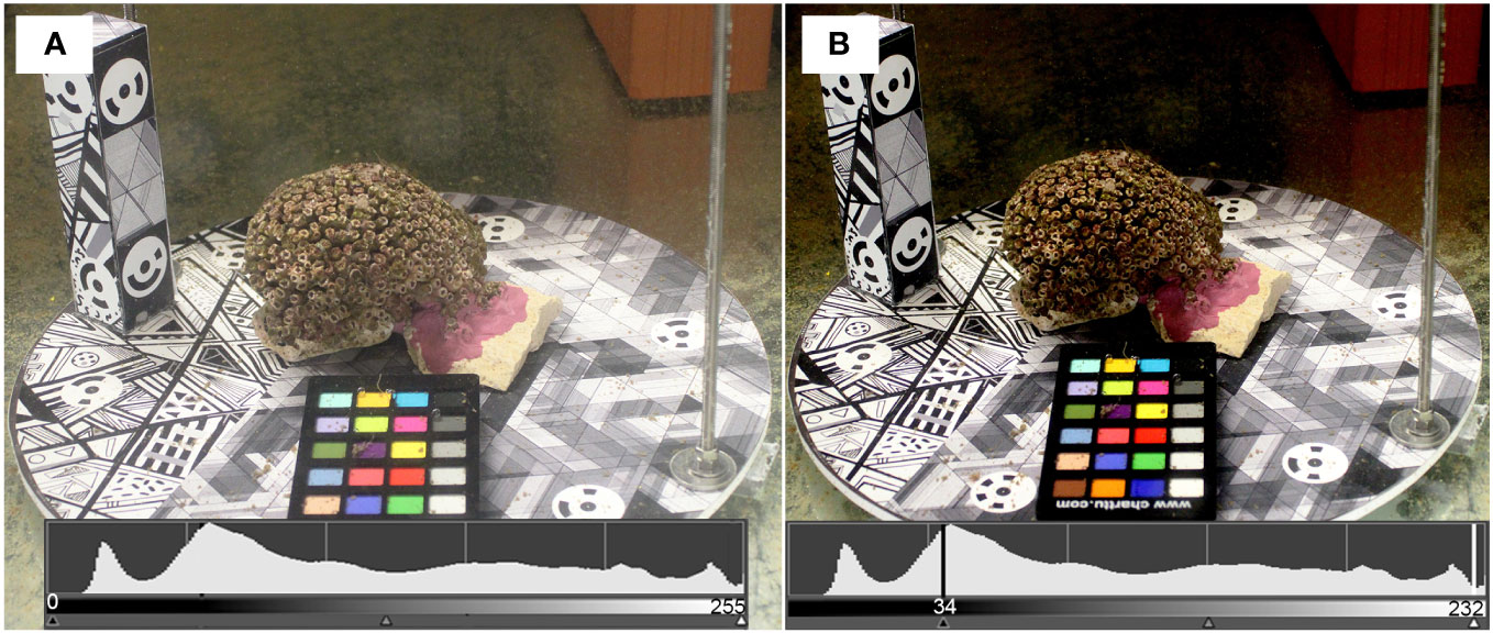
Figure 3 Results of the image enhancement process carried out using a color checker during image collection: (A) original image; (B) modified image after the white balancing process has been applied.

The metric accuracies of 3D models, shown in Table 2 as discrepancies on Ground Control Points (GCPs) coordinates and reference distances, were about 0.45 mm and 0.75 mm. The mean resolution of the 3D models ranged from 60 to 100 vertexes/mm²; these values were mainly related to the average acquisition distance that influenced the numerosity of the mesh vertexes. The generated 3D reconstructions highlighted how the anchor damages, producing a geometric change, can be detected from the model, whereas the effects of ultrasonic baths are only noticeable thanks to the high photorealistic texture of the photogrammetric model, thus from the radiometric content and not from the geometric one.

3.2 Coral morphology and biometry and polyp health status

The main descriptors of coral morphology and biometry, obtained after the analysis of planar underwater photos, are reported in Table 3. The average amount of time required to identify and count corallites depended on the size of the colony but was generally extensively long: at least 4 hours in the case of C6, which consisted of 602 corallites (Table 3), and 2.5 hours for C10 and C20 that were smaller (102 and 90 corallites in Epoch 0, respectively; Table 3). Counting was then repeated to confirm the values obtained. The same activities on the 3D models using the software Cloud Compare required 7-10 minutes for both C10 and C20, and about 35 minutes for C6, shortening the amount of time required for identifying and assessing the health state of corallites.

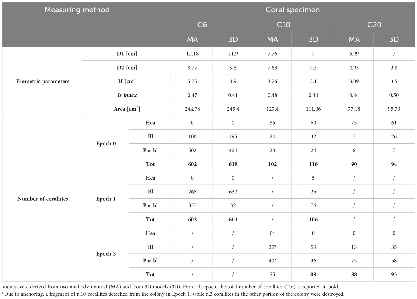
Table 3 Biometric parameters of Cladocora caespitosa (D1, D2: diameters; H: height), and number of healthy (Hea), bleached (Bl) and partially bleached (Par bl) corallites before (Epoch 0) and after (Epochs 1 and 2/3) natural degradation and mechanical stresses.

Comparing planar imaging and 3D models, in the case of C10 a total of 14 corallites were left out while counting manually, both in Epoch 0 and 1, as well as for C20 (4-5 corallites were not counted from planar images in Epoch 0 and 1), suggesting that their detection was probably prevented by the resolution and perspective of pictures (Table 3). In addition, there was a marked difference in the estimate of the state of health of C20 since about twenty corallites were considered partially bleached in planar imaging but resulted to be bleached from the 3D model (Table 3). Even for C6, the 3D model allowed the detection of a greater number of corallites than planar pictures. Besides, the application of color correction strongly favored the recognition of polyps. The corallites identified in Epoch 1 (affected just from natural bleaching and not from mechanical stresses) not only outnumbered those counted from planar pictures in Epoch 0 but were easier distinguishable from each other compared to those from the same model before color correction. Algal overgrowth covering the entire colony also made it difficult to identify the corallites beneath, but color correction resulted in emphasizing the shape of single structures and letting them emerge (Table 3).

3.3 Fluorescence analyses

Figures 4A–C shows, as an example, an $\underset{\_}{I_{compensated}}(t)$ image for each of the three epochs of the coral fragments C10. These results were obtained during 48 hours of baseline recording (Epoch 1*; Table 1) that followed the mechanical stress caused by the anchor (Epochs 2; Table 1), and 120 hours of observation following partial immersion of the colony in the ultrasonic bath (Epochs 3).

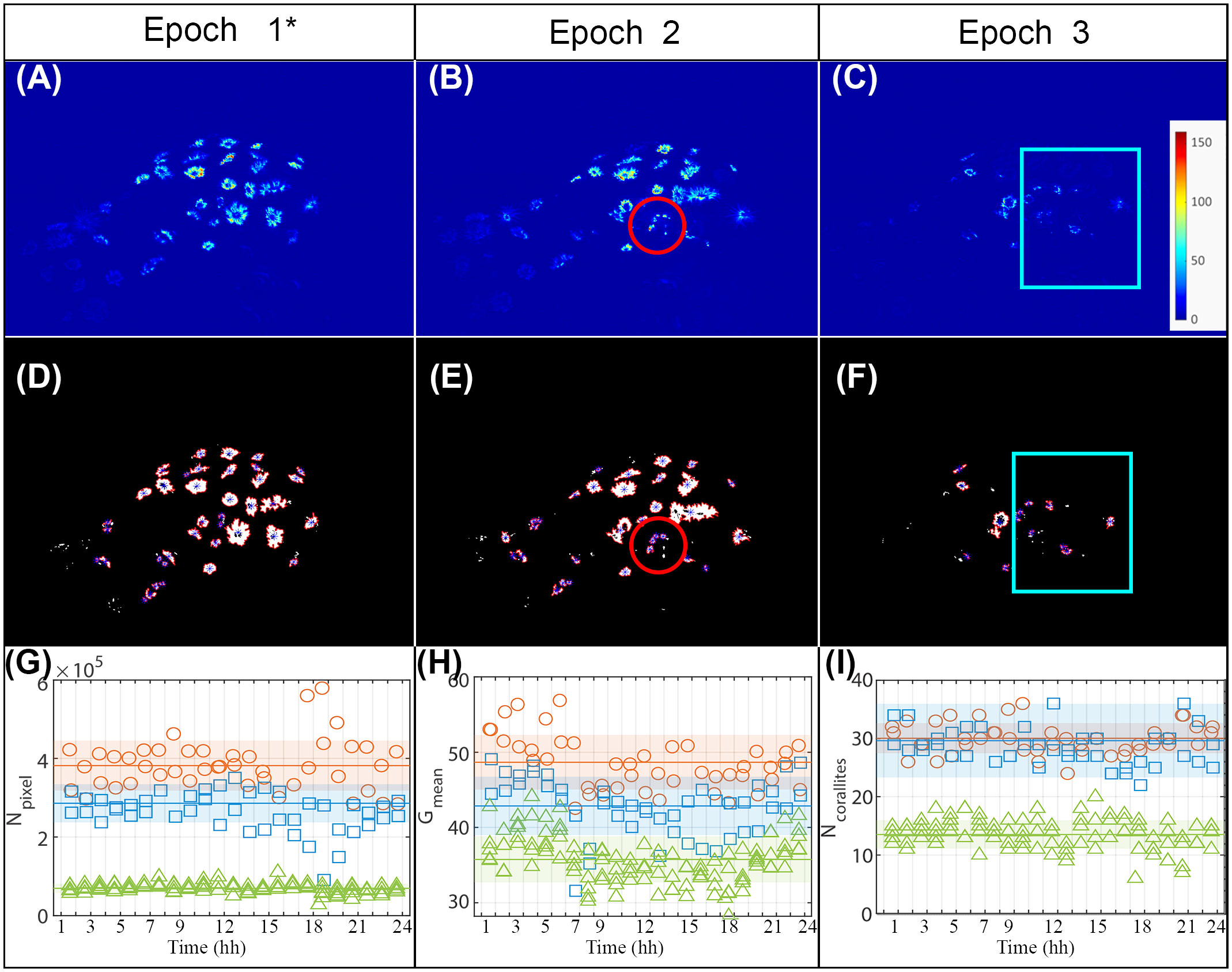
Figure 4 (A–C) Examples of an $\underset{\_}{I_{compensated}}(t)$ image for each of the three epochs; the color represents the intensity of the green levels as reported in the color bar. (D–F) Results obtained from processing the images (A–C) to identify the corallites; the blue asterisks represent the corallites centroids detected by the developed algorithm. (A, B, D, E) Red circles highlight the areas subjected to anchor damage. (C, F) Blue boxes highlight the areas subjected to ultrasonic bath. (G) Evolution over time of the number of (green) pixels above threshold, N_pixel, in the three epochs. (H) Evolution over time of the average intensity of the (green) pixels above threshold, G_mean, in the three epochs. (I) Evolution over time of the number of corallites, N_corallites, identified in the three epochs. (G, H, I) The same legend is used in all plots: orange circles refer to Epoch 1*; blu squares refer to Epoch 2 and green triangles refer to Epoch 3. Horizontal lines represent the mean of all measurements obtained in the specific epoch; the colored areas represent the range with semi-amplitude equal to the experimental standard deviation of all the observations recorded in that epoch.

Processing these images to detect the fluorescence highlighted the corallites, leading to their easier identification within the image (Figures 4D–F). Despite the significant duration of each of the observation epochs, all the proposed estimators (Figures 4G–I) showed good repeatability within the specific epoch. In this regard, it is important to note that, for each of the three epochs, multiple measurements were acquired at each of the observation times (2 acquisitions for epochs 1* and 2 and 5 acquisitions for epoch 3.

In Figures 4G–I the comparison between the images relating to Epochs 1* and 2 confirmed that the impact of the anchor displaced some of the corallites. However, at least in the short term, it did not appear to have significantly altered the state of health of the whole colony, since the number of (green) pixels above the threshold ($N_{pixel}$) and the average intensity of the (green) pixels above threshold ($G_{mean}$) displayed a similar trend. The number of corallites identified by $N_{corallites}$ remains essentially unchanged as this estimator does not discriminate between healthy and partially bleached corallites. The slight reductions in the $N_{pixel}$ and $G_{mean}$ estimators between epochs 1* and 2 are consistent with a state of distress for the corallites and the consequent partial reduction of the surface area and/or average intensity. $N_{pixel}$ and $G_{mean}$ agreed in identifying a variation between Epochs 2 and 3 (Figures 4G, H), thus after the application of the ultrasonic bath. Hence, the proposed method was able to reveal the decline in the health state of the colony after tissue degradation. $N_{pixel}$ and $N_{corallites}$ were more effective in the detection than $G_{mean}$, showing a sharp reduction in the passage between epoch 2 and epoch 3. Such a sharp reduction is observed both by comparing the measurements obtained at the different observation times and by comparing the mean values, that is, the average of all the observations obtained in the epoch. Indeed, despite the experimental standard deviations calculated on all the observations recorded in the epoch including a possible contribution of variability due to eventual physiological fluctuations in the corallites’ activity during the day, the variations in the mean values obtained in the various epochs - the horizontal lines in the Figures 4F, G, I) - are markedly greater than the respective experimental standard deviations of all the observations recorded in that epoch - the colored areas. Considering that the epochs are composed of dozens of observations each, the variation would be even more significant if compared with the experimental standard deviation of the mean (i.e., the experimental standard deviation of the observations divided by the square root of the number of observations). Hence, the detected reductions are statistically significant and, thus, reasonably attributable to an increase in the number of closed polyps, probably damaged by the stress provided.

3.4 Change detection: quantitative analysis of stresses impacts

Co-registration of 3D models for multi-temporal comparisons showed a mean error of 0.1 mm, with a standard deviation of 0.05 mm for specimen C10 (Epoch 1 vs Epoch 0 and Epoch 3 vs Epoch 0) and 0.07 mm with a standard deviation of 0.03 mm for C20 (Epoch 2 vs Epoch 0). Co-registration of 3D reconstructions of specimen C6 was not performed because deformation analysis was not implemented.

The anchor damage was recognized both in acquired images (areas highlighted with red circles in Figures 5B, C in comparison with Figure 5A) and in obtained 3D models (areas highlighted with red circles in Figures 5E, F in comparison with Figure 5D). The developed photogrammetric methodology and the high resolution of the 3D models allowed the detection of the damage: the anchor caused the break of a branch in specimen C10 at Epoch 1 and the subsequent loss of the branch. At Epoch 3 the broken chalices were well identifiable in the 3D model comparison (see the volume in gray in Figure 5I). Damages created by the ultrasonic bath were not identified with the 3D model comparison because they did not produce geometric modifications (blue box in Figure 5I); the bleaching was the only effect that could be detected in the final 3D textured meshes as well as in the captured images (blue box in Figures 5F, C respectively). The statistical analysis of the M3C2 distances, as calculated over the entire specimen, showed a mean value of 0.10 mm and a standard deviation of 1 mm for specimen C10 at both Epoch 1 vs Epoch 0 and Epoch 3 vs Epoch 0 (Figures 5H, I). The resulting mean value of the distances computed on the entire fragment was not statistically significant, confirming the global quality of the co-registration performed on stable portions. On the contrary, when locally analyzing the changes, a significant modification was detected due to the anchor damage: loss of materials up to 1 cm are highlighted in Figures 5H, I (the areas around red circles are colored in blue, according to negative distance values). Moreover, the vertical section of the three co-registered models (Figure 5G) also confirmed these results. Skewness values of computed distance distributions were smaller than1| in both cases, confirming the symmetric distribution of computed distances. The Kurtosis coefficient was equal to 70 in Epoch 2 vs. Epoch 0 and 23 in Epoch 3 vs. Epoch 0, the distribution functions of computed distances are narrow.

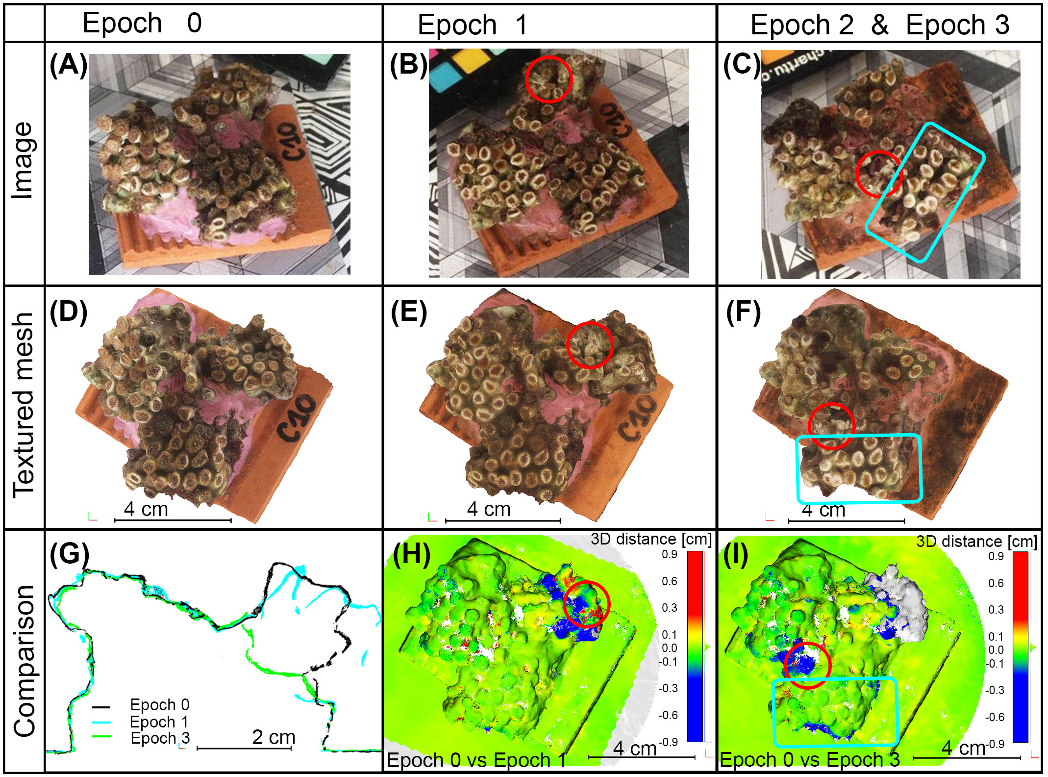
Figure 5 Results of sample C10 during the epochs of analysis. (A–C) Images captured to allow the photogrammetric reconstruction. (D–F) Top view of the generated 3D textured mesh in the specified epochs. (G–I) Examples of multi-temporal analyses. (G) Comparison of the vertical sections obtained from the final 3D reconstructions at different epochs. (H, I) Point clouds comparisons between Epoch 0 and Epoch 1 and between Epoch 0 and Epoch 3 respectively; measurements are in centimeters, blue color means loss of material, red color refers to growth. Red circles indicate the impact of the anchor; blue boxes contain areas affected by ultrasonic bath.

Multi-temporal comparison of specimen C20 pointed out that damages generated by the anchor impact were also clearly detectable in both acquired images and generated 3D models (red circles in Figures 6B, D in comparison with Figures 6A, C). Distances between 3D point clouds at Epoch 2 and Epoch 0 (red circle in Figure 6F) showed a mean value of 0.06 mm and a standard deviation of 0.80 mm; also, the area of impact was identifiable and a change greater than 3 mm up to 1 cm could be measured (red circle in Figure 6F). Skewness is 0.3 and the kurtosis coefficient was 87. The resulting statistical parameters, obtained from the M3C2 distances, also proved that the co-registration procedure was effective for the analysis of the whole specimen, and the applied stresses did not produce detectable global effects on it. The damages generated by the ultrasonic bath were not identifiable (blue box in Figure 6F). A view of the resulting 3D solid mesh is shown in Figure 6E.

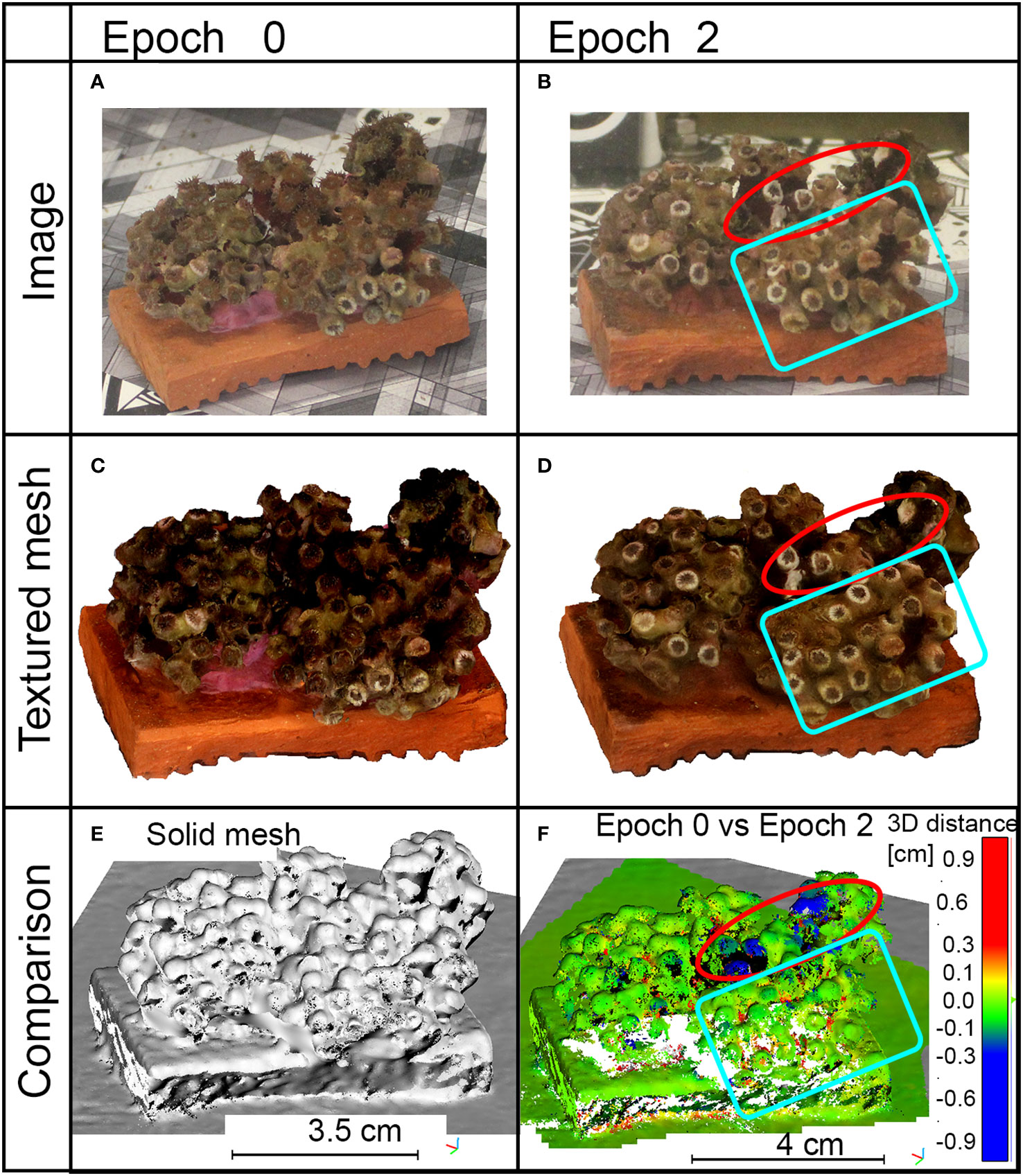
Figure 6 Results of sample C20 during the epochs of analysis. (A, B) Images captured for the photogrammetric processing. (C, D) Top view of the generated 3D textured mesh in the specified epochs. (E) Solid view of the generated mesh. (F) Point clouds comparison between Epoch 0 and Epoch 2; measurements are in centimeters, blue color means loss of material, red color refers to growth. Red circles indicate the impact of the anchor; blue boxes contain areas affected by ultrasonic bath.

4 Discussion

The crucial role of bioconstructor species in sustaining the high biodiversity and contributing to ecological processes encourages the development of new approaches and strategies for improving their knowledge and safeguarding. The measuring system developed in the present work is based on underwater photogrammetry and fluorescence imagery. The former can provide high accuracy and high-resolution 3D models to help ecologists quantify and detect changes in relevant biometric parameters, while the latter could be critical for assessing the health status of coral species.

Concerning the underwater photogrammetric dataset, the implemented strategy for frame acquisition and the GCPs network allowed the generation of 3D reconstructions with similar geometric characteristics at different epochs, in terms of resolution, accuracy, and completeness, thus guaranteeing repeatability of the analyses and the detection of local measurements of changes. The choice of autofocus, for the photogrammetric approach proposed with this paper, allowed an optimization of the acquisition of images, considering the reduced depth field. The small variations in the acquisition distance (because the camera was installed on a fixed tripod and the specimen was positioned on a plate that underwent only small rotations) did not lead to significant changes in the focal length or the estimation of the interior orientation parameters through the self-calibration process. In open-water conditions, the acquisition distance is usually subject to larger variations, so in these cases, the use of a fixed focal length is required because variations in the calculation of calibration parameters would not be negligible.

The establishment of a reference network for the accurate identification of GCPs coordinates is relevant to increase the overall significance of multi-temporal analysis. The accuracy of the implemented constraints was set up, in this study, at 0.5 mm, a precautionary value for laboratory conditions and a precise target network. External references increase the accuracy of photogrammetric products (by constraining the bundle adjustment) and ensure the repeatability of the survey in multi-temporal comparison applications. Even though in open-water conditions, the identification of stable or unchanged areas could be complex, previous in-situ activities carried out by the Authors provided helpful experiences in the installation of reliable artificial targets and the use of external references, which are highly recommended (Rossi et al., 2020) in cases where a fine scale and high accuracy monitoring is aimed. Coral monitoring is usually carried out on vast test areas that are selected on purpose to evaluate the health status and modifications occurring to multiple bioconstructor colonies over time. The measuring system proposed in this paper would not be useful for diffuse monitoring that, involving large areas, would not be devoted to providing high accuracy and fine-scale products and it would not allow the installation of targets (because it is not known a priori where disturbances will occur). The proposed system, combined with a previous installation of artificial targets, is potentially suitable for a fine-scale monitoring program at the single coral level in open water, with the final aim of succeeding in the detection of changes in coral health before lasting damages occur. Indeed, the validation in open water is out of the scope of this paper and is currently in progress within a new research project.

As an additional plus to the system developed, the definition of the state of health of corallites from laboratory measures resulted in a critical parameter to assess. Multiple images were necessary to document the whole surface of the colony but identifying the same corallites in a range of photos with different perspectives and counting them manually avoiding repetitions resulted to be extremely difficult. As revealed by the data obtained, the creation of different sectors to overcome this issue was not successful both in terms of data quality and time required for the analyses. Moreover, the thread did not remain perfectly attached to the coral structure and small corallites could be covered, while the resolution of pictures did not allow to observe macro details, affecting the counting. On the other hand, the 3D models provided detailed corallite imaging, with fine definition at a polyp scale suitable for morphological observations and change detection analysis. High-quality texture mapping in the digital mesh allowed not only the identification of corallites, Kopecky et al. (2023) also estimates living tissues, epiphyte colonization, and bleaching events thanks to the implementation of color calibration procedures. Overall, the developed measuring system is easier to use, and more effective in saving time and providing detailed corallite imaging for change detection analyses than 2D photos.

The comparison of 3D models confirmed the quality of the co-registration performed on common and stable portions of the sample. The implemented strategy for co-registration proved to be capable of properly positioning the 3D models within the same reference frame without affecting the identification of changing portions. This was confirmed by analyzing the diffuse areas where no changes occurred; in these cases, indeed, most of the calculated distances were close to zero: the average distance values for C10 and C20 specimens were in the range of co-registration error (0.10 mm); standard deviations were low and calculated values were consistent with the applied stresses. Furthermore, the effects of anchor damages were visible in the figures and exceeded the calculated standard deviation values in the impact areas only. The skewness and kurtosis coefficients suggested a symmetrical and narrow distribution of computed 3D distances. If the monitoring time and the treatments to the specimen increase, the kurtosis coefficient decreases suggesting a wider distribution (69 and 23 for Epoch 3 vs Epoch 0 and Epoch 2 vs Epoch 0, respectively). An extremely relevant issue to consider when performing multi-temporal monitoring is the significance of the calculated changes. In this study, a significant analysis of the computed distances was defined through the variance propagation law applied to the variances of the GCPs, as obtained in the photogrammetric reconstruction phase (see Table 2). For specimen C10, the distances greater than 1.10 mm and 1.50 mm were significant (at 95% level of confidence) in comparing Epoch 3 with Epoch 0 and Epoch 1 with Epoch 0, respectively. For specimen C20, the significance threshold was 1.15 mm in comparing Epoch 2 with Epoch 0. According to the implemented methodology, only the computed distances that exceeded these threshold values were considered significant modifications of the structure. These analyses confirmed what emerged in the results section (Section 3): only the areas affected by anchor damages (see red circles in Figures 5H, I, 6F) showed significant changes.

Concerning the fluorescence imagery, given the weak intensity of fluorescence, the image has a signal-to-noise ratio which is generally significantly less convenient than that of the images relating to the analysis of the reflection from the sample. Therefore, in general, the image obtained in fluorescence is less suitable for the fine reconstruction of the sample structure. On the other hand, given that studying the fluorescence of corals could provide an indicator of their health state (Roth et al., 2010), fluorescence analysis could represent significant support for the monitoring and preservation of bioconstructor species. The images obtained in fluorescence allowed an easy distinction between vital and inanimate objects, and to distinguish the healthy corallites. The three estimators proposed to quantify the coral health status, namely, N_pixel, G_mean, and N_corallites, were able to reveal the reduction of healthy corallites caused by immersion in the ultrasonic bath (Figures 4G–I). In this regard, it is important to observe that the comparison between the elaborations of the images obtained from the various epochs required that the field of view was unchanged. The number of pixels above the threshold, as well as the number of viable corallites, depends on the portion of coral observed. On the contrary, by analyzing the green value of the pixels above the threshold, the G_mean estimator was likely less sensitive to variations in the field of view. On the other hand, as evidenced by the experimental results, the G_mean estimator was also the one that provided the worst performance in revealing the reduction in coral health. The experimental results also suggested that, despite the greater computational complexity, the N_corallites estimator provided better performances in terms of discrimination capacity regarding the health status of the corals. Furthermore, being based on the counting of the number of corallites and not on the counting of pixels or the analysis of their intensity, the N_corallites estimator should be more robust towards influencing quantities, such as the motion blur, which can modify the size of the area and/or intensity of the corallites in the acquired image.

It is important to note that the fluorescence images were obtained by setting an exposure time of 4s. This exposure time is compatible with laboratory analyses, but, for field measurements, it would likely give rise to unacceptable motion blur. Therefore, for in-field applications, it would be necessary to reduce the exposure time. Such can be achieved by using more powerful illuminants (within the limits of photobleaching), sensors with greater responsivity and/or less noise, and optics with a larger aperture, that are under setting for further implementations of the system.

Overall, the current research demonstrated the success of both underwater photogrammetry and fluorescence for ecological monitoring purposes, but significant steps are still required to achieve an integration of the two techniques. The fusion of fluorescence and photogrammetric imagery to fully exploit their potentialities and assess a finer and more complete quantification of biometry and coral health status constitutes one more concern of the Authors, which is currently upgrading.

5 Conclusions

The development of automated methods and instrumentations for underwater missions is leading to a rapid extension of marine investigated areas, both in terms of spatial coverage and depth, and also enabling preventive strategies for the protection of underwater environments and species that critically need to be safeguarded, but whose exploration could be dangerous for humans. Within this scenario, the Authors have implemented a multi-sensor measuring system that could be suitably used by SCUBA divers for assessing and quantifying the biometry and the health status of marine bioconstructors. The main goal of laboratory tests was validating and assessing the success in distinguishing between damaged and healthy organisms, as well as in detecting morphological changes with a sub-millimetric resolution. The research is moving forward through the testing of the system in open water using SCUBA divers. Besides, the mounting of the system onboard a remotely operated vehicle (ROV) is underway, pursuing the acquisition of images and further data with higher rapidity. For the future direction of the research, the quality and the repeatability of the photogrammetric surveys need to be guaranteed, as required for multi-temporal and monitoring applications, even in automatic or semi-automatic conditions, with particular concern to all environments that are not safe for divers. The limiting factors, as described in the previous paragraphs, are the repetition of similar acquisition patterns and trajectories over time, the presence of stable external references that guarantee metric accuracy, and a direct comparison of the subsequent photogrammetric products. To this end, the experiments carried out by Menna et al., 2019 on the SLAM (Simultaneous Localization And Mapping) technique for underwater surveys are of considerable interest.

Data availability statement

The datasets presented in this article are not readily available because the dataset (photogrammetry and fluorescence imagery) are still used by authors for additional research projects. Requests to access the datasets should be directed to paolo.rossi@unimore.it; cristina.castagnetti@unimore.it.

Ethics statement

The manuscript presents research on animals that do not require ethical approval for their study.

Author contributions

CC: Conceptualization, Data curation, Funding acquisition, Investigation, Methodology, Project administration, Supervision, Validation, Writing – original draft, Writing – review & editing. PR: Data curation, Formal Analysis, Investigation, Methodology, Visualization, Writing – original draft, Writing – review & editing. SR: Data curation, Formal Analysis, Investigation, Methodology, Writing – original draft, Writing – review & editing. SC: Data curation, Methodology, Visualization, Writing – original draft, Writing – review & editing. RS: Conceptualization, Investigation, Supervision, Writing – review & editing. LR: Investigation, Methodology, Writing – review & editing. AC: Conceptualization, Funding acquisition, Project administration, Supervision, Writing – review & editing.

Funding

The author(s) declare financial support was received for the research, authorship, and/or publication of this article. The research was funded by University of Modena and Reggio Emilia under the 2020 and 2022 FAR Mission Oriented Calls (Fondi di Ateneo per la Ricerca): title of the projects “SIMBAD - Sistemi Innovativi di rilievo per il Monitoraggio ambientale e la ricostruzione 3D di organismi Biocostruttori mArini con Droni subacquei” and “POSEIDON - Photogrammetry, Optical SEnsors, and unmanned underwater vehIcles for non-invasive large-scale monitoring of meDiterranean benthic cOmmuNities and habitats”. The activities were also partially funded under the National Recovery and Resilience Plan (NRRP), Mission 04 Component 2 Investment 1.5 – NextGenerationEU, Call for tender n. 3277 dated 30/12/2021 Award Number: 0001052 dated 23/06/2022.

Acknowledgments

Authors would like to thank Dr. Giorgio Di Loro and Dr. Davide Cassanelli for the great help in the experimental tests concerning fluorescence imagery capturing. Moreover, Authors would like to mention the Diving Center “Under Hundred” in San Vito Lo Capo, Sicily (Italy) for crucial assistance in the field activities.

Conflict of interest

The authors declare that the research was conducted in the absence of any commercial or financial relationships that could be construed as a potential conflict of interest.

Publisher’s note

All claims expressed in this article are solely those of the authors and do not necessarily represent those of their affiliated organizations, or those of the publisher, the editors and the reviewers. Any product that may be evaluated in this article, or claim that may be made by its manufacturer, is not guaranteed or endorsed by the publisher.

References

Akkaynak D., Treibitz T. (2019). “Sea-thru: A method for removing water from underwater images,” in Proceedings of the IEEE/CVF conference on computer vision and pattern recognition (Long Beach, California), 1682–1691.
Alieva N. O., Konzen K. A., Field S. F., Meleshkevitch E. A., Hunt M. E., Beltran-Ramirez V., et al. (2008). Diversity and evolution of coral fluorescent proteins. PloS One 3 (7). doi: 10.1371/journal.pone.0002680
Antoniadou C., Pantelidou M., Skoularikou M., Chintiroglou C. C. (2023). Mass mortality of shallow-water temperate corals in marine protected areas of the North Aegean Sea (Eastern Mediterranean). Hydrobiology 2 (2), 311–325. doi: 10.3390/hydrobiology2020020
Bayley D. T., Mogg A. O. (2020). A protocol for the large-scale analysis of reefs using Structure from Motion photogrammetry. Methods Ecol. Evol. 11 (11), 1410–1420. doi: 10.1111/2041-210X.13476
Bayley D. T., Mogg A. O., Koldewey H., Purvis A. (2019). Capturing complexity: field-testing the use of ‘structure from motion’ derived virtual models to replicate standard measures of reef physical structure. PeerJ 7, e6540. doi: 10.7717/peerj.6540
Bongaerts P., Dubé C. E., Prata K. E., Gijsbers J. C., Achlatis M., Hernandez-Agreda A. (2021). Reefscape genomics: leveraging advances in 3D imaging to assess fine-scale patterns of genomic variation on coral reefs. Front. Mar. Sci. 8. doi: 10.3389/fmars.2021.638979
Burns J. H., Weyenberg G., Mandel T., Ferreira S. B., Gotshalk D., Kinoshita C. K., et al. (2020). A comparison of the diagnostic accuracy of in-situ and digital image-based assessments of coral health and disease. Front. Mar. Sci. 7 (1). doi: 10.3389/fmars.2020.00304
Burns J. H. R., Delparte D., Gates R. D., Takabayashi M. (2015). Utilizing underwater three-dimensional modeling to enhance ecological and biological studies of coral reefs. Int. Arch. Photogrammetry Remote Sens. Spatial Inf. Sci. 40. doi: 10.5194/isprsarchives-XL-5-W5-61-2015
Caldwell J. M., Ushijima B., Couch C. S., Gates R. D. (2017). Intra-colony disease progression induces fragmentation of coral fluorescent pigments. Sci. Rep. 7, 14596. doi: 10.1038/s41598-017-15084-3
Cerrano C., Danovaro R., Gambi C., Pusceddu A., Riva A., Schiaparelli S. (2010). Gold coral (Savalia savaglia) and gorgonian forests enhance benthic biodiversity and ecosystem functioning in the mesophotic zone. Biodiversity Conserv. 19, 153–167. doi: 10.1007/s10531-009-9712-5
Chimienti G., De Padova D., Adamo M., Mossa M., Bottalico A., Lisco A., et al. (2021). Effects of global warming on Mediterranean coral forests. Sci. Rep. 11 (1), 20703. doi: 10.1038/s41598-021-00162-4
Courtney L. A., Fisher W. S., Raimondo S., Oliver L. M., Davis W. P. (2007). Estimating 3-dimensional colony surface area of field corals. J. Exp. Mar. Biol. Ecol. 351 (1-2), 234–242. doi: 10.1016/j.jembe.2007.06.021
De La Torriente A., Aguilar R., Gonzalez-Irusta J. M., Blanco M., Serrano A. (2020). Habitat forming species explain taxonomic and functional diversities in a Mediterranean seamount. Ecol. Indic. 118, 106747. doi: 10.1016/j.ecolind.2020.106747
Ferrari R., Figueira W. F., Pratchett M. S., Boube T., Adam A., Kobelkowsky-Vidrio T., et al. (2017). 3D photogrammetry quantifies growth and external erosion of individual coral colonies and skeletons. Sci. Rep. 7 (1), 16737. doi: 10.1038/s41598-017-16408-z
Figueira W., Ferrari R., Weatherby E., Porter A., Hawes S., Byrne M. (2015). Accuracy and precision of habitat structural complexity metrics derived from underwater photogrammetry. Remote Sens. 7 (12), 16883–16900. doi: 10.3390/rs71215859
Forrester G. E. (2020). The influence of boat moorings on anchoring and potential anchor damage to coral reefs. Ocean Coast. Manage. 198, 105354. doi: 10.1016/j.ocecoaman.2020.105354
Forrester G. E., Flynn R. L., Forrester L. M., Jarecki L. L. (2015). Episodic disturbance from boat anchoring is a major contributor to, but does not alter the trajectory of, long-term coral reef decline. PloS One 10 (12), e0144498. doi: 10.1371/journal.pone.0144498
Gómez-Gras D., Linares C., de Caralt S., Cebrian E., Frleta-Valić M., Montero-Serra I., et al. (2019). Response diversity in Mediterranean coralligenous assemblages facing climate change: Insights from a multispecific thermotolerance experiment. Ecol. Evol. 9 (7), 4168–4180. doi: 10.1002/ece3.5045
Guo T., Capra A., Troyer M., Grün A., Brooks A. J., Hench J. L., et al. (2016). Accuracy assessment of underwater photogrammetric three dimensional modelling for coral reefs. International Archives of the Photogrammetry. Remote Sens. Spatial Inf. Sci. 41 (B5), 821–828. doi: 10.3929/ethz-b-000118990
Gutierrez-Heredia L., Benzoni F., Murphy E., Reynaud E. G. (2016). End to end digitisation and analysis of three-dimensional coral models, from communities to corallites. PloS One 11 (2), e0149641. doi: 10.1371/journal.pone.0149641
Istenič K., Gracias N., Arnaubec A., Escartín J., Garcia R. (2020). Automatic scale estimation of structure from motion based 3D models using laser scalers in underwater scenarios. ISPRS J. Photogrammetry Remote Sens. 159, 13–25. doi: 10.1016/j.isprsjprs.2019.10.007
Kersting D., Cebrian E., Verdura J., Ballesteros E. (2017). A new Cladocora caespitosa population with unique ecological traits. Mediterr. Mar. Sci. 18 (1), 38–42. doi: 10.12681/mms.1955
Kersting D. K., Cefalì M. E., Movilla J., Vergotti M. J., Linares C. (2023). The endangered coral Cladocora caespitosa in the Menorca Biosphere Reserve: Distribution, demographic traits and threats. Ocean Coast. Manage. 240, 106626. doi: 10.1016/j.ocecoaman.2023.106626
Kersting D. K., Linares C. (2012). Cladocora caespitosa bioconstructions in the Columbretes Islands Marine Reserve (Spain, NW Mediterranean): distribution, size structure and growth. Mar. Ecol. 33 (4). doi: 10.1111/j.1439-0485.2011.00508
Kopecky K. L., Pavoni G., Nocerino E., Brooks A. J., Corsini M., Menna F., et al. (2023). Quantifying the loss of coral from a bleaching event using underwater photogrammetry and AI-assisted image segmentation. Remote Sens. 15 (16), 4077. doi: 10.3390/rs15164077
Kružić P., Benković L. (2008). Bioconstructional features of the coral Cladocora caespitosa (Anthozoa, Scleractinia) in the Adriatic Sea (Croatia). Mar. Ecol. 29 (1), 125–139. doi: 10.1111/j.1439-0485.2008.00220.x
Lague D., Brodu N., Leroux J. (2013). Accurate 3D comparison of complex topography with terrestrial laser scanner: Application to the Rangitikei canyon (NZ). ISPRS J. photogrammetry Remote Sens. 82, 10-26. doi: 10.1016/j.isprsjprs.2013.04.009
Lakowicz J. R. (1992). Topics in fluorescence spectroscopy: principles (Vol. 2). Springer Sci. Business Media.
Lange I. D., Perry C. T. (2020). A quick, easy and non-invasive method to quantify coral growth rates using photogrammetry and 3D model comparisons. Methods Ecol. Evol. 11 (6), 714–726, 10–26. doi: 10.1111/2041-210X.13388
Lavy A., Eyal G., Neal B., Keren R., Loya Y., Ilan M. (2015). A quick, easy and non-intrusive method for underwater volume and surface area evaluation of benthic organisms by 3D computer modelling. Methods Ecol. Evol. 6 (5), 521–531. doi: 10.1111/2041-210X.12331
Marre G., Holon F., Luque S., Boissery P., Deter J. (2019). Monitoring marine habitats with photogrammetry: a cost-effective, accurate, precise and high-resolution reconstruction method. Front. Mar. Sci. 276. doi: 10.3389/fmars.2019.00276
Menna F., Nocerino E., Fassi F., Remondino F. (2016). Geometric and optic characterization of a hemispherical dome port for underwater photogrammetry. Sensors 16 (1), 48. doi: 10.3390/s16010048
Menna F., Nocerino E., Nawaf M. M., Seinturier J., Torresani A., Drap P., et al. (2019). “Towards real-time underwater photogrammetry for subsea metrology applications,” in OCEANS 2019-Marseille (Marseille: IEEE), 1–10. doi: 10.1109/OCEANSE.2019.8867285
Menna F., Nocerino E., Remondino F. (2017). Flat versus hemispherical dome ports in underwater photogrammetry. Int. Arch. Photogrammetry Remote Sens. Spatial Inf. Sci. 42, 481–487. doi: 10.5194/isprs-archives-XLII-2-W3-481-2017
Million W. C., O’Donnell S., Bartels E., Kenkel C. D. (2021). Colony-level 3D photogrammetry reveals that total linear extension and initial growth do not scale with complex morphological growth in the branching coral, Acropora cervicornis. Front. Mar. Sci. 8. doi: 10.3389/fmars.2021.646475
Nocerino E., Menna F. (2023). In-camera IMU angular data for orthophoto projection in underwater photogrammetry. ISPRS Open J. Photogrammetry Remote Sens. 7, 100027. doi: 10.1016/j.ophoto.2022.100027
Nocerino E., Menna F., Gruen A., Troyer M., Capra A., Castagnetti C., et al. (2020). Coral reef monitoring by scuba divers using underwater photogrammetry and geodetic surveying. Remote Sens. 12 (18). doi: 10.3390/rs12183036
Nocerino E., Menna F., Verhoeven G. J. (2022). Good vibrations? How image stabilisation influences photogrammetry. Int. Arch. Photogrammetry Remote Sens. Spatial Inf. Sci. 46, 395–400. doi: 10.5194/isprs-archives-XLVI-2-W1-2022-395-2022
Oakley J. P., Satherley B. L. (1998). Improving image quality in poor visibility conditions using a physical model for contrast degradation. IEEE Trans. image Process. 7 (2), 167–179. doi: 10.1109/83.660994
Price D. M., Robert K., Callaway A., Lo Lacono C., Hall R. A., Huvenne V. A. (2019). Using 3D photogrammetry from ROV video to quantify cold-water coral reef structural complexity and investigate its influence on biodiversity and community assemblage. Coral Reefs 38, 1007–1021. doi: 10.1007/s00338-019-01827-3
Ramesh C. H., Koushik S., Shunmugaraj T., Murthy M. R. (2019). A rapid in situ fluorescence census for coral reef monitoring. Regional Stud. Mar. Sci. 28, 100575. doi: 10.1016/j.rsma.2019.100575
Righi S., Prevedelli D., Simonini R. (2020). Ecology, distribution and expansion of a Mediterranean native invader, the fireworm Hermodice carunculata (Annelida). Mediterr. Mar. Sci. 21 (3), 558–574. doi: 10.12681/mms.23117
Rodolfo-Metalpa R., Peirano A., Houlbrèque F., Abbate M., Ferrier-Pagès C. (2008). Effects of temperature, light and heterotrophy on the growth rate and budding of the temperate coral Cladocora caespitosa. Coral Reefs 27, 17–25. doi: 10.1007/s00338-007-0283-1
Rossi P., Castagnetti C., Capra A., Brooks A. J., Mancini F. (2020). Detecting change in coral reef 3D structure using underwater photogrammetry: critical issues and performance metrics. Appl. Geomatics 12, 3–17. doi: 10.1007/s12518-019-00263-w
Roth M. S., Latz M. I., Goericke R., Deheyn D. D. (2010). Green fluorescent protein regulation in the coral Acropora yongei during photoacclimation. J. Exp. Biol. 213 (21), 3644–3655. doi: 10.1242/jeb.040881
Roveta C., Coppari M., Calcinai B., Di Camillo C. G., Marrocco T., Pulido Mantas T., et al. (2023). What’s the key for success? Translocation, growth and thermal stress mitigation in the Mediterranean coral Cladocora caespitosa (Linnaeus 1767). Front. Mar. Sci. 10. doi: 10.3389/fmars.2023.1199048
Sasano M., Imasato M., Yamano H., Oguma H. (2016). Development of a regional coral observation method by a fluorescence imaging LIDAR installed in a towable buoy. Remote Sens. 8 (1), 48. doi: 10.3390/rs8010048
Sobha T. R., Vibija C. P., Fahima P. (2023). ““Coral reef: A hot spot of marine biodiversity”,” in Conservation and Sustainable Utilization of Bioresources. Eds. Sukumaran S. T., , K T. R. (Singapore: Springer Nature Singapore), 171–194.
Teague J., Megson-Smith D. A., Allen M. J., Day J. C., Scott T. B. (2022). A review of current and new optical techniques for coral monitoring. Oceans 3 (1), 30–45. doi: 10.3390/oceans3010003
Treibitz T., Neal B. P., Kline D. I., Beijbom O., Roberts P. L., Mitchell B. G., et al. (2015). Wide field-of-view fluorescence imaging of coral reefs. Sci. Rep. 5 (1), 7694. doi: 10.1038/srep07694
Ventura D., Dubois S. F., Bonifazi A., Jona Lasinio G., Seminara M., Gravina M. F., et al. (2021). Integration of close-range underwater photogrammetry with inspection and mesh processing software: a novel approach for quantifying ecological dynamics of temperate biogenic reefs. Remote Sens. Ecol. Conserv. 7 (2), 169–186. doi: 10.1002/rse2.178
Wang Y., Song W., Fortino G., Qi L. Z., Zhang W., Liotta A. (2019). An experimental-based review of image enhancement and image restoration methods for underwater imaging. IEEE Access 7, 140233–140251. doi: 10.1109/ACCESS.2019.2932130
Keywords: underwater photogrammetry, fluorimetry, biometry, marine bioconstructors, optical sensors, 3D dense models, change detection
Citation: Castagnetti C, Rossi P, Righi S, Cattini S, Simonini R, Rovati L and Capra A (2024) Potentialities of the combined use of underwater fluorescence imagery and photogrammetry for the detection of fine-scale changes in marine bioconstructors. Front. Mar. Sci. 10:1305807. doi: 10.3389/fmars.2023.1305807
Received: 02 October 2023; Accepted: 18 December 2023;
Published: 08 January 2024.
Edited by:
John H. R. Burns, University of Hawaii at Hilo, United StatesReviewed by:
Atsuko Fukunaga, University of Hawai’i at Mānoa, United StatesFabio Menna, Bruno Kessler Foundation (FBK), Italy
Copyright © 2024 Castagnetti, Rossi, Righi, Cattini, Simonini, Rovati and Capra. This is an open-access article distributed under the terms of the Creative Commons Attribution License (CC BY). The use, distribution or reproduction in other forums is permitted, provided the original author(s) and the copyright owner(s) are credited and that the original publication in this journal is cited, in accordance with accepted academic practice. No use, distribution or reproduction is permitted which does not comply with these terms.
*Correspondence: Paolo Rossi, paolo.rossi@unimore.it