Calcification, Dissolution and Test Properties of Modern Planktonic Foraminifera From the Central Atlantic Ocean

1 Introduction

Calcium carbonate (CaCO₃) production and its export to the deep ocean is one of the most important sinks for carbon and alkalinity across a range of geological timescales (Zeebe and Westbroek, 2003). This CaCO₃ cycling thus affects atmospheric pCO₂ and also plays a fundamental role in regulating ocean chemistry and pH – a major factor in the viability of calcareous marine organisms. In the modern ocean, biogenic CaCO₃ comprises the vast majority of marine carbonate production, being mainly supplied by foraminifera, coccolithophores, pteropods and coral reef ecosystems (Ridgwell and Zeebe, 2005). This biogenic production and export of calcite is controlled by three principal components: (1) changes in the abundance of calcifying versus non-calcifying taxa, (2) changes in the efficiency of the in/organic carbon export and burial, and (3) changes in the calcification efficiency of marine calcifiers (Archer and Maier-Reimer, 1994; Hofmann et al., 2010), and these factors are sensitive to environmental conditions (Barker and Elderfield, 2002; McClelland et al., 2016; Zarkogiannis et al., 2019a). Since the exact nature of this environmental sensitivity remains unclear, it is difficult to quantify the impact of future climate change on calcium carbonate production. Consequently, studies that focus directly on the mass of the fossilized shells of the calcifiers such as foraminifera are essential.

Planktic foraminifera, which live in the ocean surface layers from tropical to polar regions, contribute 32–80% of the total deep-marine calcite budget in the global carbonate cycle (Schiebel, 2002). Individual species of planktonic foraminifera preferentially live in specific water masses and depths to which they adapt according to oceanic inhomogeneity (Emiliani, 1954; Mortyn and Charles, 2003). The ability of non-motile plankton to inhabit specific depths in the water column requires a means of regulating buoyancy and foraminifera may have different strategies (e.g., low-density metabolic products) for short-term displacement or micro-positioning in the water column, such as any diurnal migrations (Hemleben et al., 1989). For longer term regulation of vertical habitat depth, shell density control during biomineralization provides an inert way for non-motile plankton to regulate flotation and increase negative buoyancy (Marszalek, 1982; Campbell and Dower, 2003) as it grows larger during the long term, ontogenic vertical decent (Meilland et al., 2021).

Through their journey in the water column, planktonic foraminifera shells also provide a record of past changes in surface seawater properties or surface frontal movements. A good understanding of the function of the shells in living plankton is however fundamental in order to avoid any misinterpretation of their significance in relation to paleooceanography and paleoclimatology. Although the effects of ocean chemistry on plankton shells are being extensively studied today, there is a void of information in the literature about the effects of physical oceanic properties such as buoyancy or pressure, which very likely affect plankton physiology and morphology (Lipps, 1979). These organisms are able to biosynthesize out of equilibrium with their ambient environment by maintaining chemical gradients (de Nooijer et al., 2009; Toyofuku et al., 2017; Evans et al., 2018), but as non-motile plankton they cannot go against water density gradients and they must always retain equilibrium with the seawater to remain afloat. In order to inhabit certain depths, planktonic foraminifera should regulate their density to match that of the surrounding liquid in which they are immersed. Should this not be the case, then the organisms will relocate until they reach a particular density horizon to equilibrate. It can thus be argued that plankton physiology may be more sensitive to the physical rather than the chemical characteristics of seawater.

In the present study we closely examine the physical properties of shells of different planktonic foraminifera species by looking at their mass variations and changes in their architecture. The weight of the shells of several planktonic species from a core-top sample set are investigated together with their meridional and bathymetric changes across the central Atlantic. In order to assess the preservation state of the shells and further explore their physical and spatial properties, test specimens of several species were analyzed using high resolution X-ray microcomputed tomography. The tomographic analyses allowed the normalization of the shell masses to the total cell volume and determination of a measure of bulk shell density – an estimate of skeletal concentration of the foraminifera cell. The aim was to evaluate the meridional and bathymetric changes in the mass of the planktonic foraminifera shells that are associated with their calcification during growth in the water column and subsequent dissolution on the seafloor.

2 Materials and Methods

A meridional transect of 16 Atlantic core-top samples was assembled to examine the weight of the mass of modern planktonic foraminifera shells over a large, ocean-basin scale hydrographic gradient (Figure 1A). The samples span from 31°N to 25°S and their locations are situated along either flank of the Mid-Atlantic Ridge to capture open ocean conditions from cores across a narrow depth range (∼2.9 to ∼3.7 km) from the North, Equatorial, and South Atlantic. This depth range was chosen as it contained the greatest number of available cores in the three regions, and it is consistently above the ∼4 km lysocline depth (Berger, 1968), enabling us to examine shell weight differences that may be driven by factors other than the $\text{Δ}{\text{CO}}_3^{2-}$ [defined as ${\left({\text{CO}}_3^{2-}\right)}_{\mathrm{insitu}-}$ ${\left({\text{CO}}_3^{2-}\right)}_{\text{saturation}}$] of bottom waters. The samples consist mainly of foraminiferal marl ooze and correspond to a range of upper water column structures, varying from a strongly stratified, shallow thermocline at the equator to a much thicker, mixed surface layer at the subtropical gyres. We divide our core-tops into “equatorial” (between 10°S and 10°N) and “extra-equatorial” (north of 10°N and south of 10°S) regions, according to the annual mean surface temperature or density (Figures 1B, C). Various criteria ensure the late Holocene age of the core-tops (see Arbuszewski et al., 2010; Cléroux et al., 2013 for details).

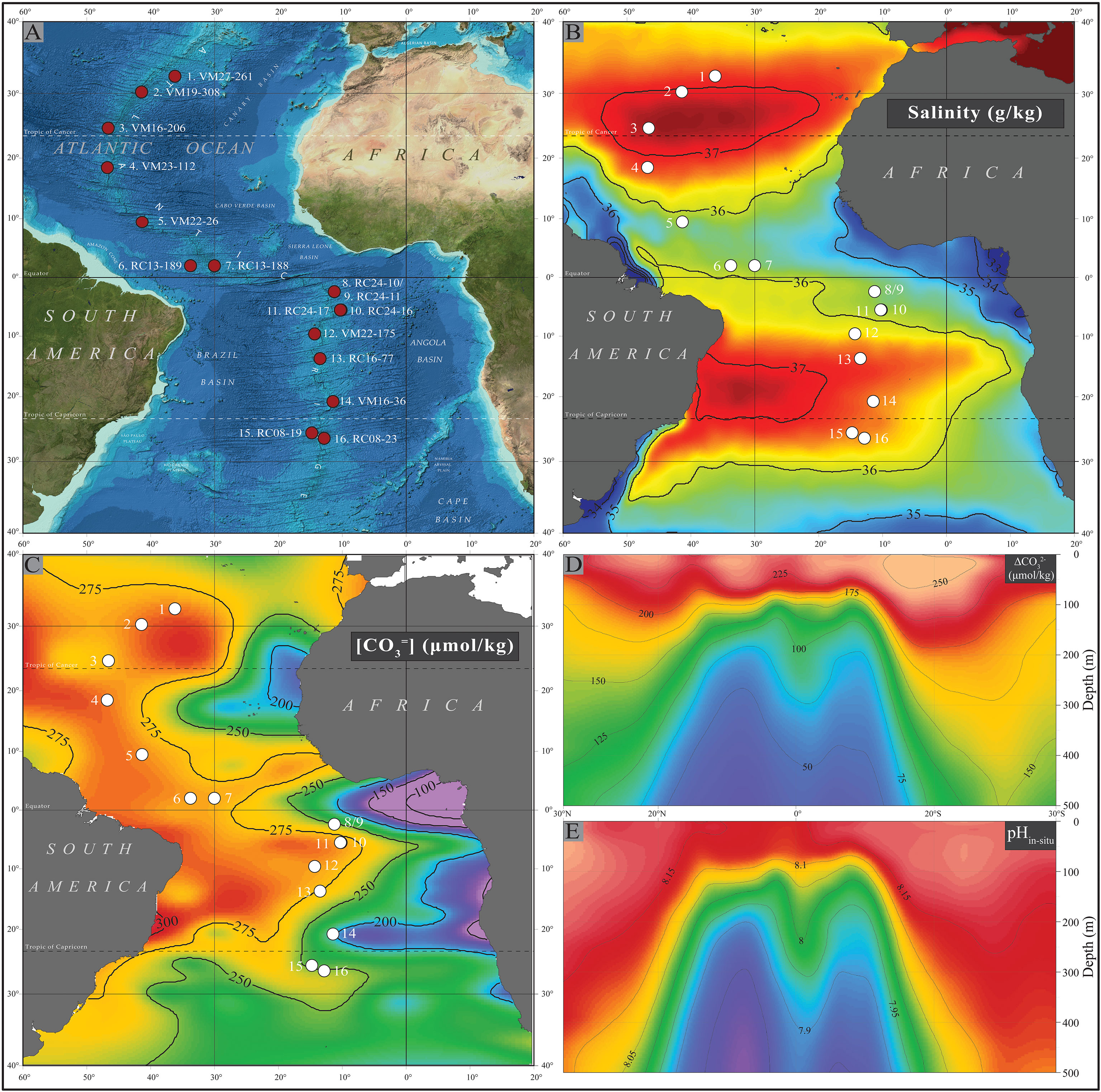
Figure 1 (A) Locations of the 16 core-top samples for this study; (B) mean annual SSS (PSU). Data from the World Ocean Atlas 2013; (C) preindustrial surface seawater [${\text{CO}}_3^{2-}$] (μmol/kg); Latitudinal hydrographic sections of the central Atlantic showing preindustrial: (D) water column pH and (E) seawater saturation state with respect to calcium carbonate $\text{Δ}{\text{CO}}_3^{2-}$ estimates from GLODAP v.1 data corrected for anthropogenic dissolved inorganic carbon (Key et al., 2004).

2.1 Species Selection and Shell Mass Weights

Species were selected according to two criteria: abundances in the samples and depth habitat variety according to previous studies. Normal forms of Orbulina universa (NCBI:txid46134), Globigerinoides ruber albus (NCBI:txid2606480) sensu stricto morphotype, Globigerinoides ruber rosea (NCBI:txid2606481), Trilobatus trilobus (WoRMS:lsid1027267), Trilobatus sacculifer (WoRMS:lsid1026286), Globorotalia truncatulinoides (NCBI:txid69029), and Neogloboquadrina dutertrei (NCBI:txid51039) were picked from the 300–355 µm sieve fraction, without taking into account test coiling direction. However, the G. ruber albus morphotypes were carefully distinguished since they are known to have different habitats (Aurahs et al., 2011), with G. elongatus precipitating tests in colder surface waters than G. ruber albus sensu stricto (Steinke et al., 2005; Antonarakou et al., 2015). From every sample between 30 to 50 specimens of each species were picked and weighed in a pre-weighed aluminum carrier using a Sartorius CP2P microbalance with a precision of ±1 μg. Average sieve-based shell weights (SBW) were calculated by dividing the recorded mass by the total number of weighed specimens. Subsequently, the specimens were weighed in batches of 5 individuals in order to estimate the standard shell mass deviations. For comparisons shell weight analyses were performed on a narrow size fraction that is commonly used in paleoceanography. Performing weight analyses on a narrow foraminifera size fraction constrains the ontogenic stage of the specimens to a certain number of chambers, and thus minimizes size-related weight differences (e.g. Broecker and Clark, 2001; Barker et al., 2004; Beer et al., 2010). The analytical error, estimated by triplicate measurements of 50 random specimens, ranged from 0.42 to 0.58 μg, which is in accordance with the error of the balance.

2.2 High Resolution X-Ray Computed Microtomography

To better interpret the changes in foraminifera test weights, for each sample a number of specimens used for the above weight measurements were analyzed using computed microtomography (μCT). More specifically, 10 specimens of the surface dwelling, spinose species G. ruber (white) and 10 specimens of the deep dwelling, non-spinose G. truncatulinoides were scanned using a GE/Phoenix v|tome|x s 240 CT scanner. In addition, 2 more species (spinose T. trilobus and non-spinose N. dutertrei) were scanned from sample 8 (RC24-10), where the lowest shell weights were recorded. The tests were fixed in a customized cylindrical container as described in Zarkogiannis et al. (2020a). Embedded in the base of the container was a calcite microcrystal, which was used to standardize the computed tomography (CT) number of the scanned specimens. A high-resolution setting (voltage of 80 kV, current 80 μA, detector array size of 1024×1024, 1501 projections/360°, 2.5 s/projection) enabled the acquisition of 3D images with an isotropic pixel size of about 1.2 μm. Phoenix datos|x 2.0 software was used to correct and reconstruct tomographic data, that uses the general principle of Feldkamp cone beam algorithm to reconstruct image cross sections from the filtered back projections. XMCT not only allows the examination of the internal structure (or internal degradation) of the calcite mass, providing a means to directly assess shell disintegration due to dissolution but it also offers valuable 3D information about test biometry and thus foraminifera physiology. This 3D information together with the test mass weight measurements allowed for the first time the determination of volume normalized shell weight or foraminifera shell bulk density (see section 2.2.2).

2.2.1 Shell Preservation

Besides XMCT, the conventional Fragmentation Index (F.I.) of the coarse fraction (>150 μm) was counted (Berger, 1968) as an indication of sedimentary carbonate preservation. The F.I is calculated by the ratio of foraminifera fragments to whole tests at a 300 particles sample split and it is considered as an (indirect) indication of dissolution on the basis that increased fragmentation of tests is directly related to dissolution. A problem inherent with this index is that it is not solely related to dissolution, but also to ecologic factors such as shell thickness or mineralogy and other sedimentological issues (e.g. degree of bioturbation). Thus although F.I. may provide a measure of shell fragility, it cannot be considered a reliable (foraminiferal) dissolution proxy. In order to gain insight into the three-dimensional mass density distribution of the studied foraminiferal tests and to inspect their integrity and evaluate their degree of dissolution, the tests were tomographically assessed according to Iwasaki et al. (2015).

2.2.1.1 Test Relative Density (Mean CT Number)

The CT scan deals with the attenuation of the X-rays as they pass through materials of different density. Areas of high density (visually as opaque) like pristine calcite have high attenuation and are displayed as bright on CT, whereas areas of low density have little attenuation and are displayed as dark. From the 16-bit grayscale tomographic 3D scanning data a CT (attenuation) number was obtained for each voxel (μm³) of each individual scanned test, after removal by segmentation of detritus infill material. The 3D imaging software Molcer Plus (White Rabbit Corp., version 1.35) and the following equation were used to calculate the calcite CT number:

where μ_sample, μ_air, and μ_calciteSTD are the X-ray attenuation coefficients of the sample, air and calcite, respectively. The mean CT numbers for calcite standard and air were defined as 1000 and 0, respectively.

The mean CT number for an entire test was calculated with the following equation:

where n is the CT number, T_n is the total number of voxels with a specific CT number (n), and T is the total number of voxels in the whole test. The mean CT number indicates the mean relative density of an individual test (see section 2.2.2).

The mean CT numbers of the foraminiferal tests were sometimes larger than that of the calcite standard (1000) in the present analysis. We assumed that these results are due to a beam-hardening effect on the calcite standard. Beam hardening is an artifact associated with CT scanning caused by polychromatic radiation as the X-ray beam passes through the material. However, if the CT numbers of all foraminiferal tests are equally standardized by the same calcite standard, the CT numbers of the test specimens can be validly compared.

2.2.1.2 %Low-CT Volume (CTX)

The progressive dissolution corrodes the foraminifera test internally (Johnstone et al., 2010) creating voids in their mass producing areas of low X-ray attenuation. The voxels (volume) of low-CT number calcite relative to that of the whole test reflects the degree of disintegration and thus the extent of calcite dissolution (Iwasaki et al., 2015). In this study, we defined low-CT-number calcite and high-CT-number calcite to be associated with CT numbers of 200–500 and 500 or greater, respectively. The percentage of the low-CT-number voxels to the total number of voxels of the whole calcite test is used in the current study as a Computed Tomography dissolution indeX (CTX) and is calculated as follows:

2.2.2 Spatial XMCT Data Analysis

Besides information on material densities, subject to the quality of segmentation, XMCT can offer spatial information of high precision and accuracy to allow the study of the three-dimensional mass distribution of the scanned foraminiferal tests. The calcite test of the foraminifera was isolated from any detritus infill to give the volume of the calcite (Figure 2A). The infilling was further segmented separately. The internal cavities of each test (incorporating any infilling, to represent the true internal space) were automatically segmented (using ambient occlusion, Avizo 2020.2). The internal cavities volume and the volume of the calcite test were subsequently added to determine the volume of the whole foraminifera cell (Figure 2B). The volume occupied by detrital infilling contamination was also calculated as a percentage of the total shell volume (Zarkogiannis et al., 2020c). Mean shell thicknesses were calculated by dividing the test volume by the test surface area, both of which are parameters measured by the CT image analysis software. The shell surface area includes both the outer areas and the surfaces of the internal chambers and test pores. A caveat with the calculated mean shell thickness is that values will decrease, when the shell material is more porous. High porosity of the shell material increases the surface area, resulting in a decrease in mean shell thickness.

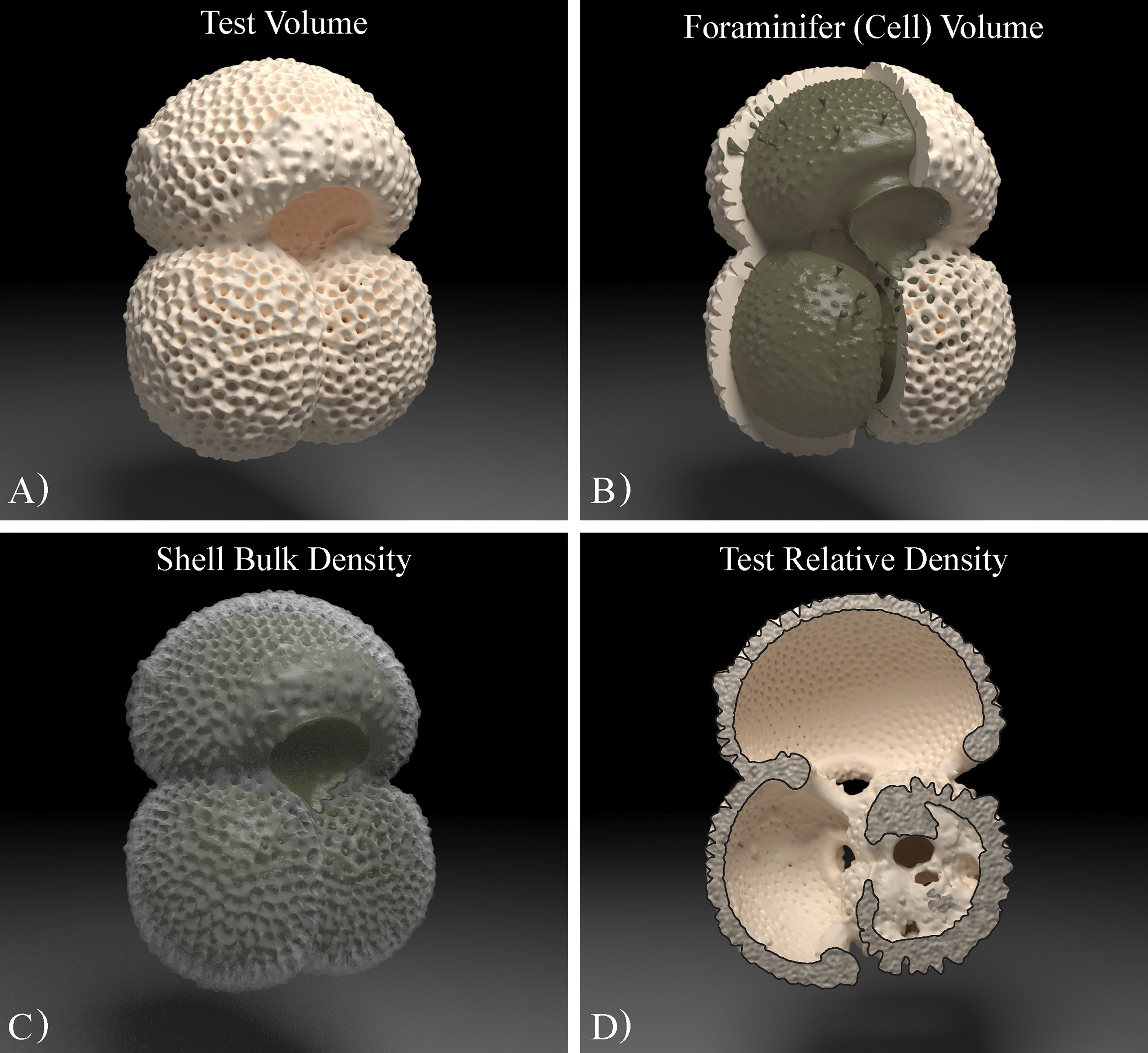
Figure 2 Three-dimensional photo-realistic imagery of a foraminifer using computer graphics rendering illustrating concepts of its skeletal spatial arrangements (excluding spines): (A) Test volume refers to the volume that the calcite biomineral occupies; (B) Cell volume is the mean volume enclosed within the exterior perimeter of the test wall and it is the sum of the calcite test volume and that of the internal cavities that are filled with protoplasm in a living cell; (C) Shell bulk density or volume normalized shell weight is the concentration of skeletal material within a foraminifera cell; (D) Test relative density is the test’s CT density compared to the CT density of the calcite standard.

The results of the visualization analyses, when combined with the shell weight measurements gave rise to some concepts that may more accurately describe characteristic qualities of fossil foraminifera cells. In this study, we term shell bulk density ρ_shell (skeletal density) the ratio of the mass of solid test material as weighed, to the sum of the volumes of the solid material and closed (or blind) cavities within the structure of the test (Figure 2C). We refer to foraminifera cell density as the ratio of the sum of the mass of the solid (test) material and the non-solid organic material (protoplasm) of a living cell to the sum of the volumes of the solid and non-solid material that occupy all voids within a living cell (total foraminifera volume; Figure 2B). At optimum living depth the cell density is equal to the ambient seawater density (see section 2.3). Furthermore, we refer to test density as the ratio of solid test mass to the solid test volume (Figure 2A), and as test relative density (Figure 2D) to the ratio of solid test X-ray attenuation (CT density) to the attenuation (CT density) of the mineral calcite. Test density may be a measure of test porosity, while test relative density can serve as a test dissolution or test mineralogical purity index.

2.3 Determination of Foraminifera Cell Density at Depth of Immersion

Foraminifera may have different means to increase their positive buoyancy (osmoregulation, lipid or metabolic gases production and storage) but biomineralization is their only mechanism to actively add negative buoyancy. Thus, the amount of heavy calcite mineral secretion determines the deepest point that foraminifera can penetrate into the water column when alive. At their optimum depth of immersion, foraminifera attain an equilibrium position in the water column. Since they are non-motile plankton, in order to occupy certain optimum depths, foraminifera should adjust their cell density to match that of the surrounding fluid at a certain point along the pycnocline. Should this not be the case then displacement occurs until the body and medium densities equilibrate. At the equilibrium point the weight force of the living foraminifer (W_foram) is equal to the weight of the liquid that it displaces (i.e. buoyancy force, B) or since both of these forces depend on the volume of the living foraminifera V_foram and the gravitational acceleration (g) the density of the whole foraminifera shell ρ_foram is equal to the density of the seawater ρ_sw, and ρ_foram is the sum of shell bulk density ρ_shell and cytoplasm density ρ_cyt. Thus:

It is possible to reconstruct the cytoplasmic density ρ_cyt if ρ_sw and ρ_shell are known. Here an attempt was made to calculate foraminifera protoplasm densities for the two different species that were X-ray scanned. Test weights of G. ruber and G. truncatulinoides were converted to shell bulk densities ρ_shell using the XMCT spatial data and ρ_sw at each species apparent living depth was calculated by fitting geochemically reconstructed calcification temperatures/depths from the literature to the Argo potential density profile data. For G. truncatulinoides ambient seawater densities were extracted at the calcification depths reported by Cléroux et al. (2013). For G. ruber ambient seawater densities were extracted from the depth horizons dictated by the calcification temperatures of Arbuszewski et al. (2010). Because the Mg/Ca analyses in Arbuszewski et al. (2010) are debated (Hertzberg and Schmidt, 2013; Dai et al., 2019), we used the δ¹⁸O-derived calcification temperatures (T_iso). For the 3 northernmost and the 3 southernmost samples from the subtropical gyres the T_iso were fitted to the average Argo profile data of the 3 warmest months of the year as suggested by Hertzberg and Schmidt (2013).

2.4 Description of Geochemical Data

The previously published geochemical data referred to throughout this paper were reported by Arbuszewski et al. (2010) for G. ruber and by Cléroux et al. (2013) for G. truncatulinoides. In both these studies a superset of 64 core-top sediment samples spanning from 31°N to 25°S along the Mid-Atlantic Ridge were analyzed for δ¹⁸O and Mg/Ca ratios for each species. These geochemical measurements were performed on wider or larger sieve fractions than the 300-355μm that was used in the present study, but still remain reliable calcification depth indicators. In brief, 80–100 specimens of G. ruber albus (sensu stricto) were picked from each sample from the 250–355 μm size fraction and between 10 and 25 specimens G. truncatulinoides dextral from the 355–425 µm fraction, then crushed and split into aliquots for Mg/Ca and δ¹⁸O analyses. After removal of clays, and full reductive and oxidative cleaning steps, samples were analyzed for Mg/Ca ratios on an ICP-OES. Samples for δ¹⁸O analyses were also cleaned in rinses of ultra-pure water prior to analysis (Arbuszewski et al., 2010; Cléroux et al., 2013).

2.5 Oceanographic Data

Mean annual and monthly ocean temperature and salinity data of the period between January 2004 and January 2020 were extracted for each core site from the International Argo Ocean Monitoring Program (Argo, 2000). The values are quality-controlled and refer to data of the first 1000 m of the water column. Instead of extrapolating single-point hydrographic data at the exact core coordinates, the surface (2.5m) temperature and salinity values of each site was extracted from a grid area of 0.1×0.1 decimal degrees (~10×10 Km) around the site location.

Ocean carbonate system data were taken from GLODAPv1.1 (Key et al., 2004). Given the late Holocene age of the core tops, we correct the modern seawater data for the acidifying influence of anthropogenic CO₂, by subtracting the GLODAPv1.1 anthropogenic DIC estimates from the total DIC values to give an estimate of pre-industrial DIC. These values, along with paired alkalinity, nutrient, and hydrographic data, were used to make pre-industrial CO₂ system determinations for GLODAP using CO2sys.m v1.1 (van Heuven et al., 2011). This dataset was then imported to Ocean Data View (Schlitzer, 2002) and carbonate system variables obtained for each site at a range of depths using Ocean Data View’s 3D estimation tool. For consistency further oceanographic parameters (salinity, temperature, density) were calculated for the same depth ranges.

3 Results

3.1 Oceanographic Regime

The Argo temperatures and corresponding salinities of the waters overlying each sample site were plotted against each other as the temperature (T) – salinity (S) diagram of Figure 3 and some of their water mass characteristics may be inferred. In terms of static stability at the sites, stratification is stable and does not overturn locally since the density increases with the depth. In the gyres, where water mass formation takes place by sinking of surface water along isopycnal surfaces, the T-S curve is a straight line; while the curvature is an indication of diapycnal mixing of (three) water masses (Sverdrup et al., 1942). The waters masses of the north Atlantic (green curves) have distinct curves and denote North Atlantic Central Waters (Araujo et al., 2011) that are denser due to their higher salinities, while the rest of the samples were bathed in South Atlantic Central Waters.

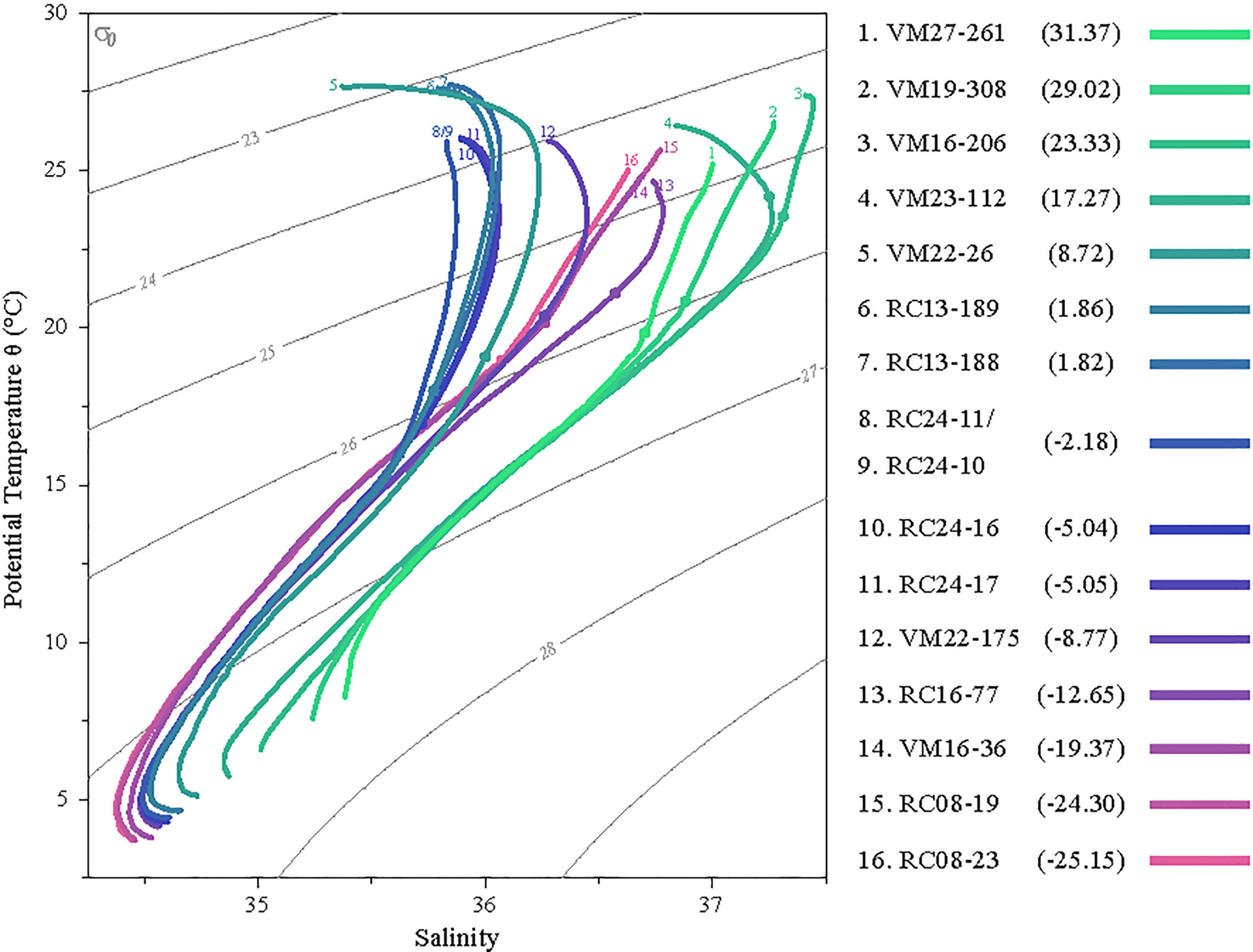
Figure 3 T-S diagram of the water masses overlying the sampling sites. The dots in each curve denote 100m depth. The shaded grey contours are isopycnals every 1σ_θ. Sample latitudes are given in the parentheses.

While for most of the sites the T-S curves have a strong curvature in the upper ~100m, indicating distinct surface water hydrography, the water of the three northern- and the three southern-most sites form straight lines, that are indicative of more active mixing of surface and subsurface waters. This is particularly true for most of the water column of the southern sites, while in the northern-most sites the slope of the curves changes at about 100m, indicating a diversification in the water masses. Sites 6-11 are below low salinity surface waters, and within the equatorial upwelling belt. The shallowest thermocline (widest temperature range for the first 100m) is found over sites 8 and 9, where the equatorial upwelling is strongest along the western margin of the African continent. Site 5 (VM22-26) is particularly affected by the river Amazon discharge exhibiting the lowest salinities for the first 30 m.

3.2 Shell Weights

The weight of the shells of foraminifera are found to be a function of their depth habitat (Figure 4). Spinose surface-dwelling species are found to be lighter than the deep dwelling non-spinose ones. O. universa was found to be the lightest species followed by G. aequilateralis and G. ruber albus. G. ruber rosea produce in general heavier shells than G. ruber albus but they are both lighter than the Trilobatus group. N. dutertrei produces the heaviest specimens in this working sieve fraction, while in some locations it is competing in being the heaviest with G. truncatulinoides, which in most cases is slightly lighter. Within the same sieve fraction, there is a 150% difference in the average shell masses between the shells of O. universa (avg. 13.6 ± 2.6 μg) and those of N. dutertrei (avg. 33.9 ± 3.4 μg). The shell weight variability for each species between the samples was on average 9%. O. universa was found to have the greatest shell weight variability (19%) along the transect. G. ruber rosea with 7% variation (Table S1) is the most consistent surface dweller in weight, while the deep dwelling G. truncatulinoides varied only 6% in the central Atlantic. Due to close similarity in weights, data from T. trilobus and T. sacculifer were averaged together and are referred to as Trilobatus group. However, for a better agreement between test weight and species-specific depth habitat the size of the shell should be accounted for and thus (SBW) shell mass measurements should be normalized to cell volume (see section 3.3).

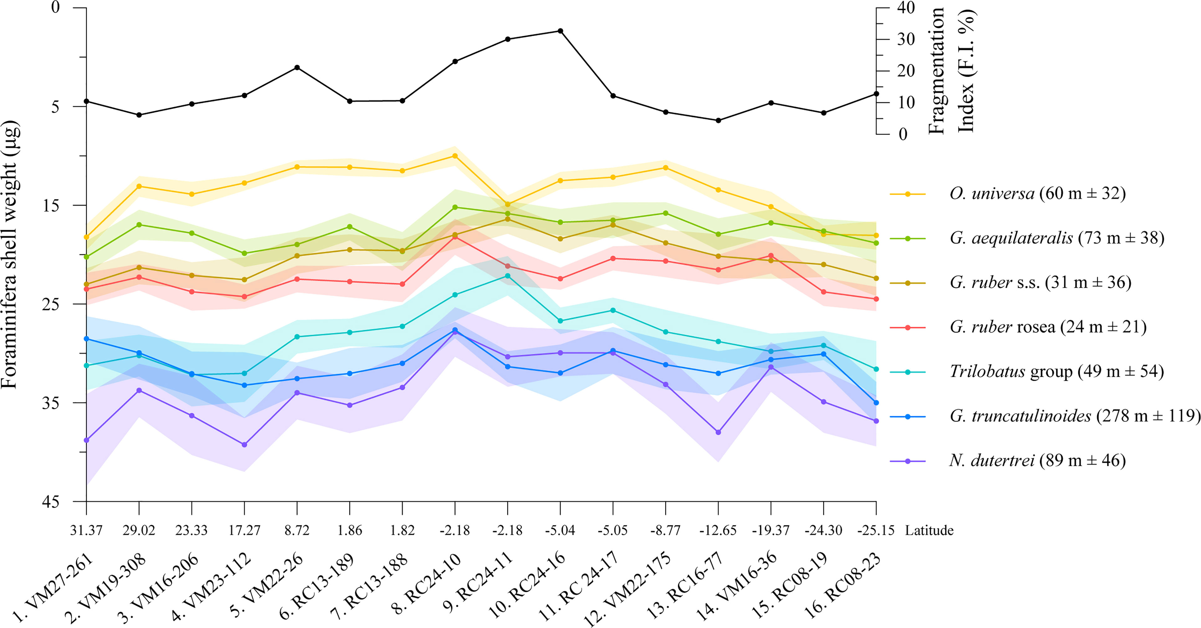
Figure 4 Average sieve-based shell weights of 7 planktic foraminifera species along the studied latitudinal transect together with the shell Fragmentation Index that was counted in the fine sand fraction (>150 μm) of the samples. Due to weigh similarity, T. trilobus and T. sacculifer were averaged together and are referred to as Trilobatus group. The shaded areas depict the 1σ confidence interval of the shell weight measurements. Numbers in the parentheses to the right show the range of preferential habitat depths for each species in the region from the literature (Anand et al., 2003; Cléroux et al., 2007; Farmer et al., 2007; Steph et al., 2009; Rebotim et al., 2016; Venancio et al., 2017; Lessa et al., 2019; Rebotim et al., 2019).

Fragmentation of specimens shows a peak in tropical waters but remains relatively mild even in the samples with the highest value [33% in sample 10 (RC 24-16)], implying relatively good preservation. By averaging the shell weights of all species for each sample (Table 1) we find the lowest shell weights in sample 8 (RC24-10), while shell fragmentation was average. Shells decrease in weight by approximately 34% from the extratropical regions of the high salinity gyres to the fresher equatorial zone, when comparing the maximum recorded weights at the extratropics to the minimum in the equatorial regions. The highest contrast in test weight measurements between these regions was recorded for O. universa (82%) and the lowest for G. truncatulinoides (27%). The contrast for G. ruber albus and T. trilobus is 40% and 45% respectively, while for N. dutertrei and T. sacculifer it is 41% and 49%. G. ruber rosea and G. aequilateralis shells varied only by 7% between the equatorial and extra-equatorial sites. When shell weight measurements of all species for each site are pooled together and are divided by the number of the weighed species, an average shell weight for the foraminifera population can be determined (Table 1). The largest difference in the average population weight of 34% is between the equatorial sample 8 and that of the S. Atlantic gyre (sample 16). The population average SBW has almost equally moderate correlation with sea surface density (R² = 0.27, p<0.05) and salinity (R² = 0.26, p<0.05), though not with sea surface [${\text{CO}}_3^{2-}$], and a hind of an anticorrelation with temperature (Supplementary Figure 1). This negative relation to temperature is due to the lighter shell weights in the warmer tropical waters and is in line with observations of a negative temperature impact of temperature on foraminifera calcification (Titelboim et al., 2021). In contrast, comparing data averaged over the range of habitat depths of most species (0-100 m) shows a strong correlation with salinity (R² = 0.54, p<0.01) a relatively strong correlation with ${\text{CO}}_3^{2-}$ (R² = 0.36, p<0.05) and no correlation with seawater density or temperature (Supplementary Figure 2).

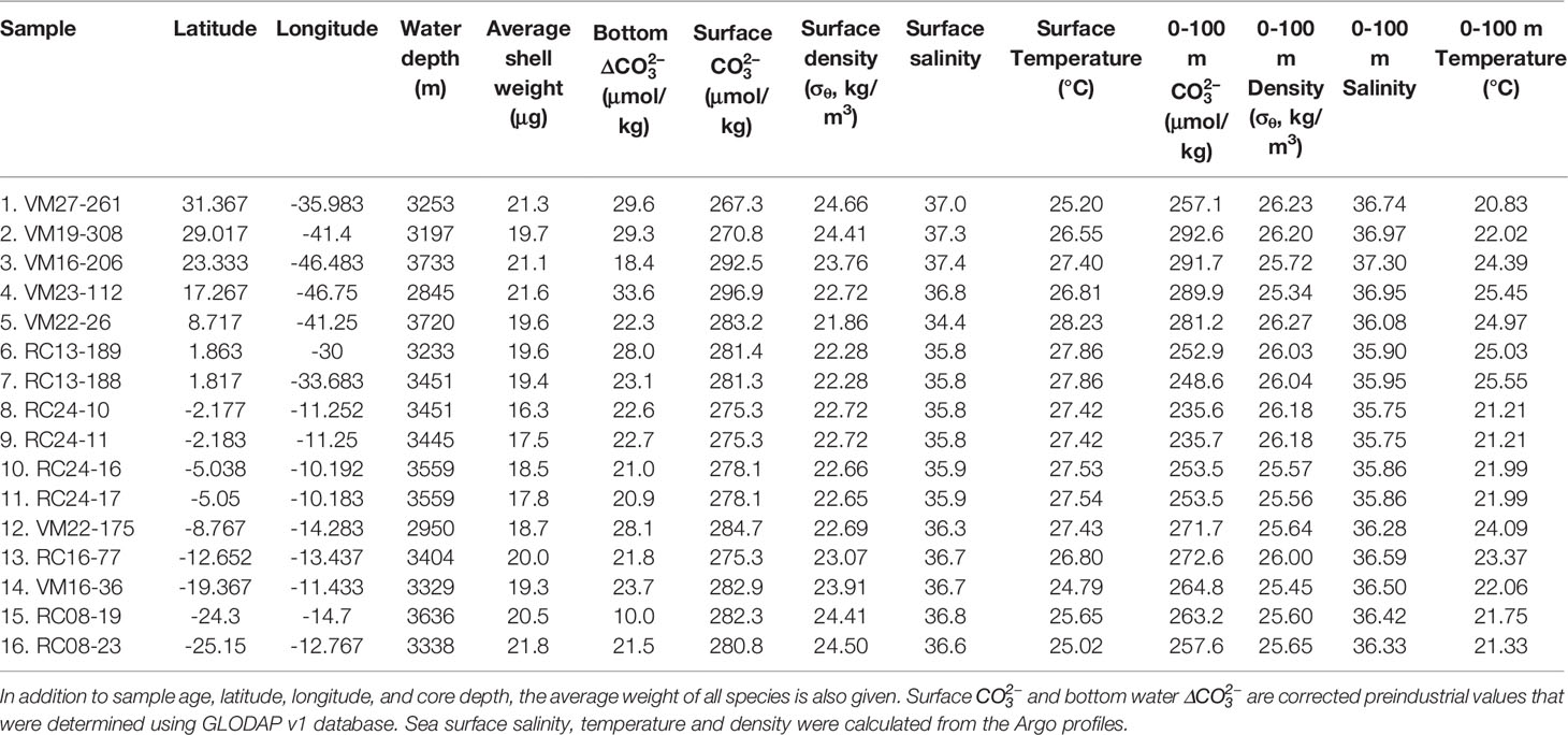
Table 1 Table of cores from which core-top samples were obtained for shell weight analyses.

3.3 Foraminifera Bulk Shell Densities

Since foraminifera are unicellular organisms with an exoskeleton, the extent of their test primarily defines their cell size. The determination using XMCT of the total volume that their cells occupy allowed the normalization of the measured test weights to the space over which the test is distributed. This allows the determination of shell bulk density or shell density in short (Figure 2C), which is measure of skeletal concentration, and is expressed in μg/μm³ or more practically in g/cm³. The calculated shell densities of G. ruber albus and G. truncatulinoides along the study transect are shown in Figure 5. Shell (bulk) densities are refinements of sieve-based shell weights and thus follow the shell weight trends of Figure 4. G. ruber shells are denser in the higher latitudes, while their density decreases at the tropical sites. G. truncatulinoides shells on the other hand although they are consistently dense in extratropics, their density varies considerably in the tropics. Vertically, shell densities increase from G. ruber albus to G. truncatulinoides to fit the depth habitat preferences of each species. This is better manifested by sample 8 (RC24-10) from which the shell densities of 4 different species were calculated. Shell bulk densities increase from G. ruber albus to T. trilobus to N. dutertrei to G. truncatulinoides, following the known calcification depths of these species in the Atlantic (Anand et al., 2003; Steph et al., 2009; Cléroux et al., 2013; Rebotim et al., 2016; Lessa et al., 2019; Rebotim et al., 2019).

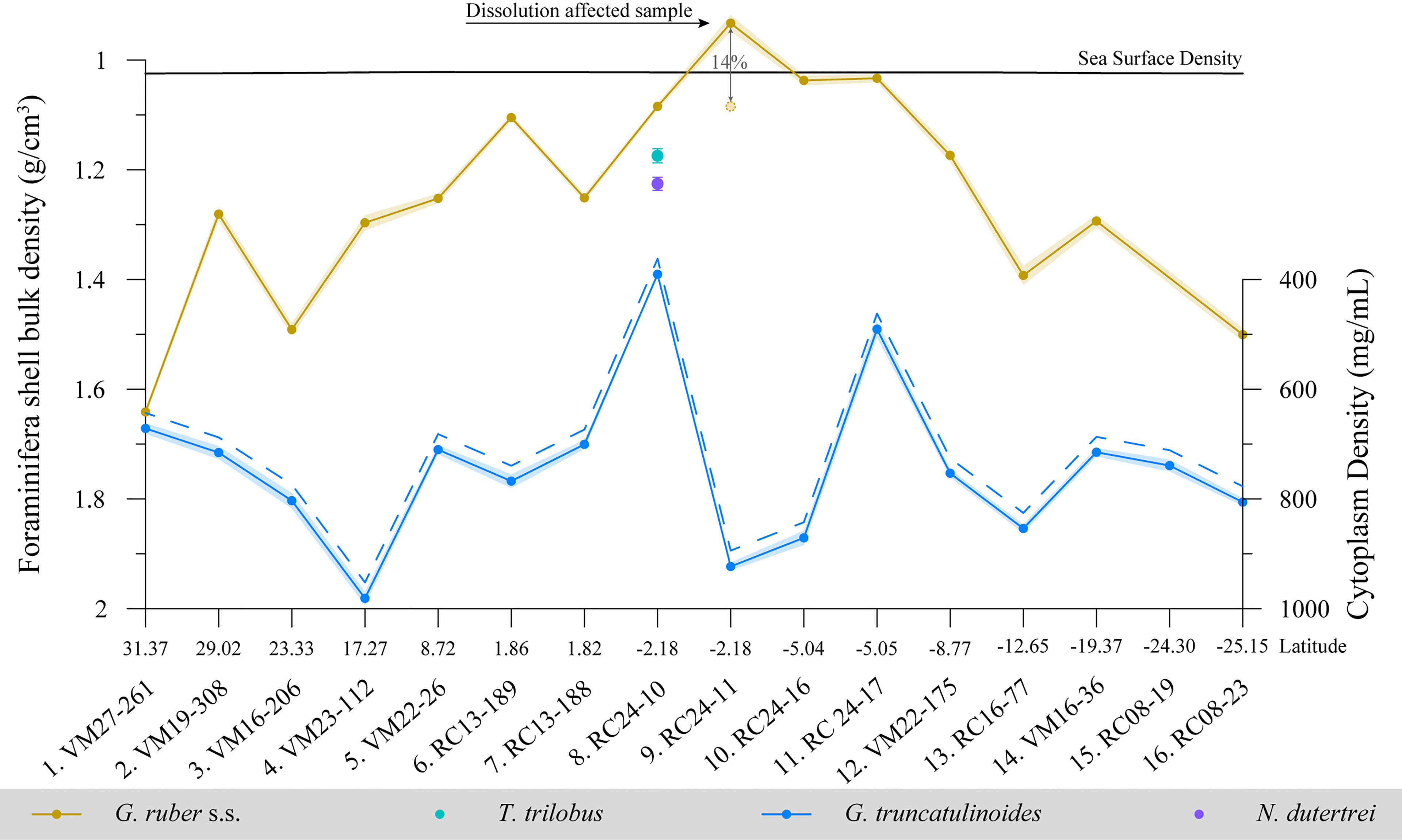
Figure 5 Shell bulk densities of four different foraminifera species. With solid lines are the bulk densities of G. ruber albus and G. truncatulinoides along the transect. The shaded areas depict the 1σ confidence interval of the shell bulk density measurements. The secondary y-axis and the dashed lines show the reconstructed average cytoplasmic densities necessary for free floating at calcification depth at each site. For sample 8. RC24-10 shell bulk densities were calculated for two additional species. In solid black line the sea surface density (SSD) is shown. The deviation of sample 9. RC24-11 from the SSD may point to test dissolution.

According to the estimates from sample 8, T. trilobus shell density is ~8% higher, while that of N. dutertrei and G. truncatulinoides are increased by 14% and 28% respectively. The average shell density of G. ruber albus specimens is 1.251 ± 0.198 g/cm³, while for G. truncatulinoides 1.743 ± 0.147 g/cm³, and both are higher than Sea Surface Density (SSD), which along the transect is 1.023 ± 0.001 g/cm³. However, for sample 9 (RC24-11) G. ruber albus shell density was found as low as 0.933 g/cm³, which is lower than the SSD. This deviation of shell density from sea water may possibly allow the quantification of dissolution. This low-density reconstruction is due to the low average shell weights of sample 9 (16.4 μg). Such low weights may be the result of dissolution and if shell bulk densities of sample 9 were between that of sample 8 and 10 then we estimate that ~14% or 2.7 μg of test calcite has been dissolved.

Another useful application of the determination of foraminifera shell bulk densities is that it allows estimates of total protoplasm mass densities. Foraminifera protoplasm densities necessary for free floating (neutral buoyancy) at calcification depth densities were calculated from Eq. 4 and are shown in Figure 5 with a dashed line. G. ruber albus protoplasm was estimated to be on average 249 mg/mL, which is s similar to human cells (Kim and Guck, 2020) but showed considerable variation (74%). In some samples the protoplasm densities were estimated as low as 9 mg/mL for the equatorial upwelling samples. We concluded that these values are artificially low, and they might be the result apparent buoyancy gained by the spines and/or the upwelling water velocities that force foraminifera to non-equilibrium density horizons within the mixed layer and are not plotted here (see discussion section 4.4). For the non-spinose species G. truncatulinoides protoplasm densities were reconstructed to be on average 715 mg/mL and less variable (21%) that agree with previous rough estimates (Marszalek, 1982).

3.4 Specimen Preservation

The results of the X-ray attenuation analyses of G. ruber albus specimens are shown in Figure 6. The relative densities (mean CT number) of G. ruber albus tests are variable along the transect but they are overall increased, especially for specimens from the southern sites. The lowest densities are found at the tropical sites (samples 9-10; Figure 6A). The statistical analyses show that G. ruber albus relative test densities do not follow sieve-based shell weights but show some correlation with (volume normalized weights) ρ_shell (R² = 0.27, p<0.05). Furthermore, although for G. truncatulinoides mean test weights did not correlate with relative test densities, test bulk density showed some moderate correlation (R² = 0.32, p<0.05) to relative test density. Since foraminifera undergo ontogenetic vertical migration to greater depths (Meilland et al., 2021), the recorded mean CT values (relative densities) of G. ruber (~960) according to the study of Ofstad et al. (2021) point to adult specimens that have lived deeper in the water column, which is line with the geochemically reconstructed calcification depths considered in the present study and denote specimens in their late ontogenic stage.

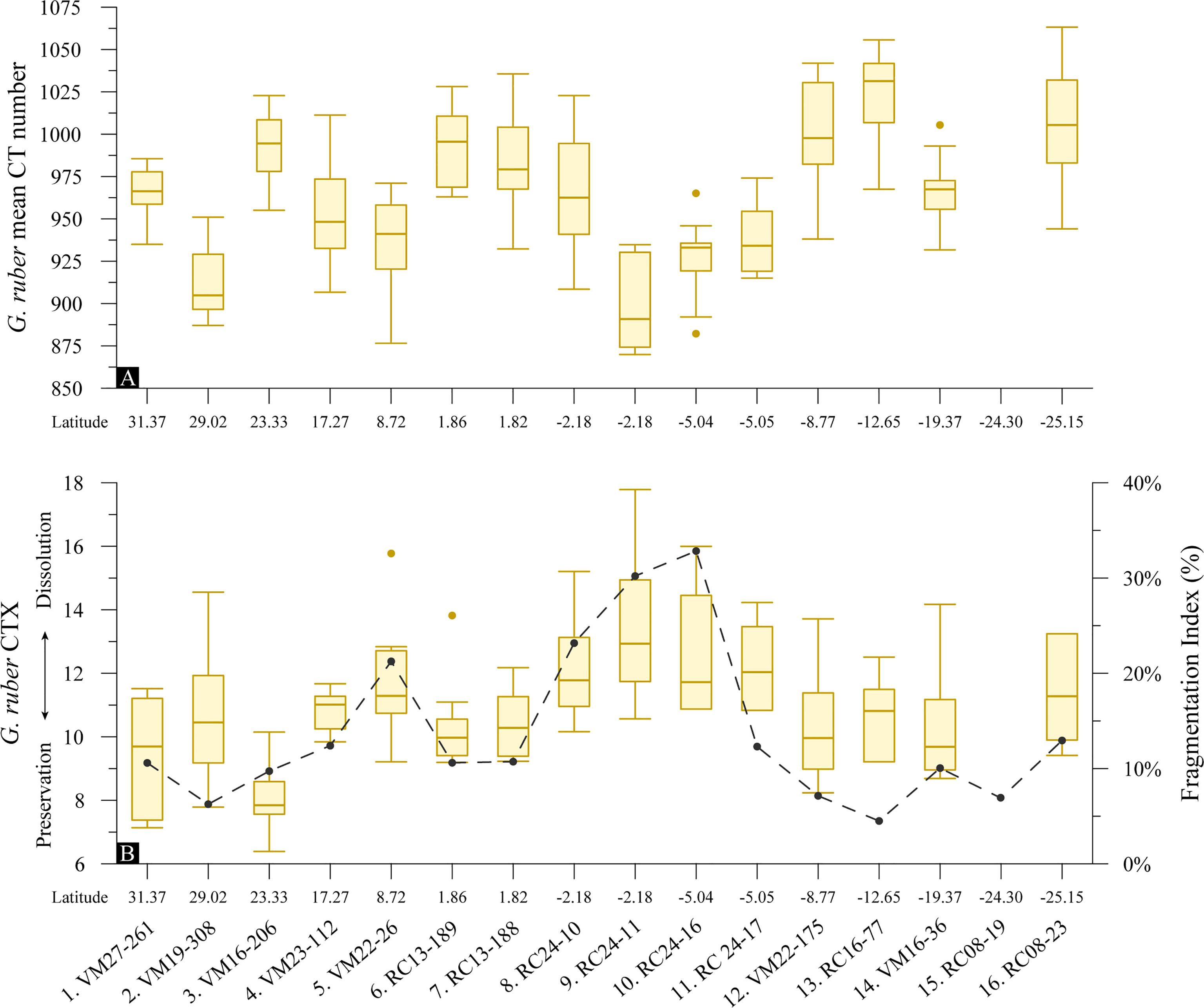
Figure 6 Box-and-whisker plots of foraminifera test (A) mean CT number indication test relative densities and (B) CTX dissolution index of the specimens with latitude for G. ruber albus (n = 152) superimposed with the planktonic foraminifera Fragmentation Index. Boxes extend from the lower to upper quartile values of the data, with a line at the median. Whiskers indicate 1.5 times the inter-quartile distance. Dots are outliers.

The percentage of low attenuation voxels within G. ruber albus test volumes (CTX) is relatively low along the transect (Figure 6B) denoting good preservation of the sedimentary calcite foraminifera tests. In contrast to the northern equatorial samples, CTX within specimens is increased in the 4 southern equatorial samples. This is in line with the decreased mean CT numbers of these samples. The generally low X-ray attenuation suggests low relative test densities that may be the result of poor preservation. However, all of the specimens retain the higher magnesium juvenile chambers (Sadekov et al., 2005) that are most susceptible to dissolution and hence they are only moderately dissolved (Johnstone et al., 2010). The highest dissolution of up to ~18% CTX by volume is recorded at sample 9 (RC24-11). Based on the CT images (Supplementary material) nearly half of the specimens from this sample show slight internal disintegration of shell walls, which is a sign of dissolution. In most samples the percentage of low X-ray attenuation regions is around 10%, while the variability of preservation between specimens is higher in the South Atlantic. The samples below the North Atlantic subtropical gyre show the best preservation. Specimen fragmentation (F.I) appears to be more related to test relative density (p <0.05) than test dissolution-CTX (p < 0.10). Furthermore, although mean shell weights were found to be only moderately correlated (p <0.05) to CTX, bulk shell densities (i.e. volume normalized shell weights) were found to be significantly (p <0.01) controlled by dissolution CTX.

The results of the X-ray attenuation analyses of G. truncatulinoides specimens are shown in Figure 7. The relative test densities of G. truncatulinoides are similar to that of G. ruber but less variable along the transect. They are overall high and like G. ruber the calcite is densest at the southernmost sites (Figure 7A). The lowest densities are recorded in sample 2 (VM19-308) from the north subtropical gyre for which G. ruber relative test densities are low as well. G. truncatulinoides test relative density was not found to be a function of mean shell weight, bulk shell density or bottom water [${\text{CO}}_3^{2-}$] (p >0.10). Furthermore, like G. ruber the calculated mean CT numbers denote specimens in their late ontogenic stage (Ofstad et al., 2021).

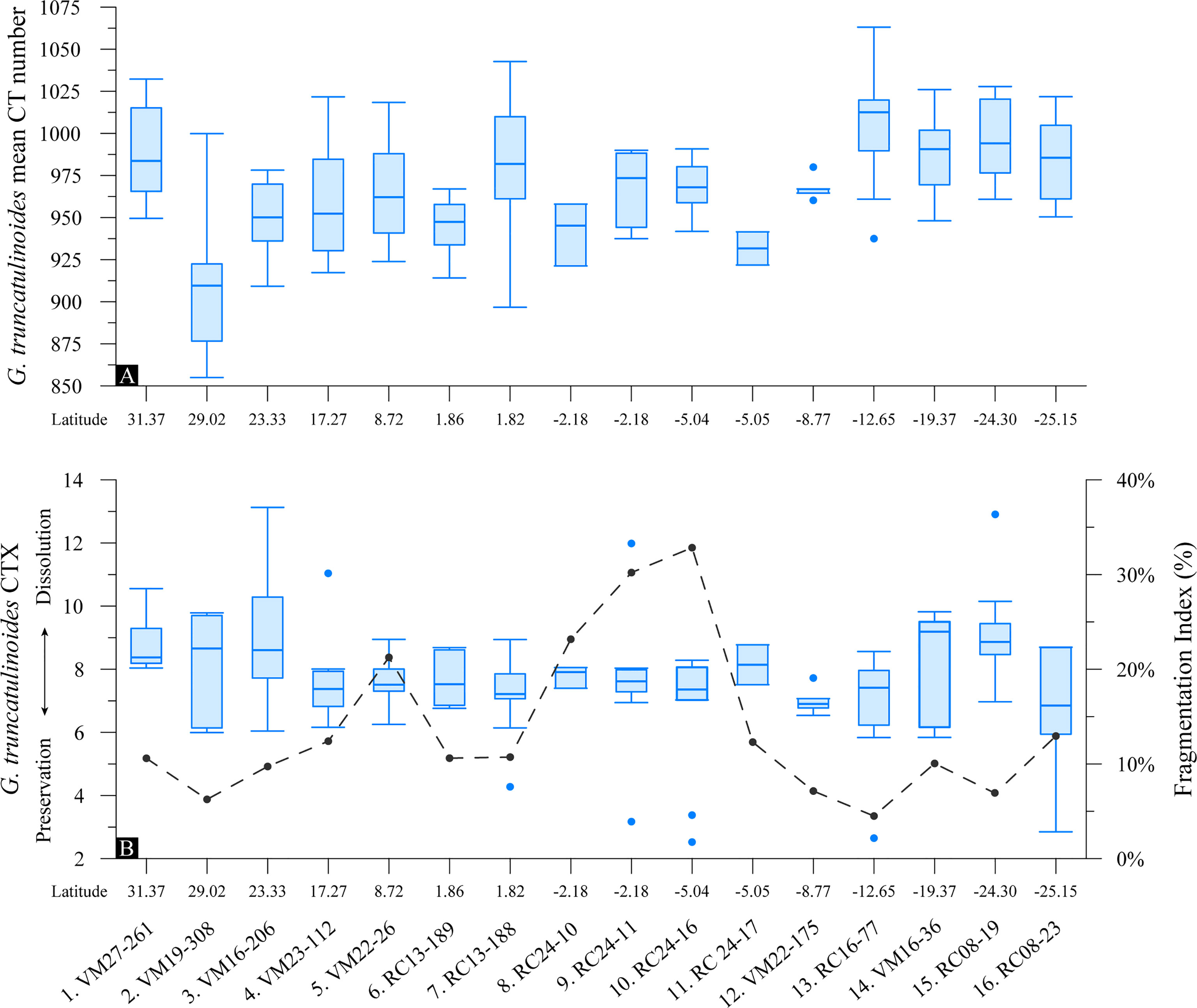
Figure 7 Box-and-whisker plots of foraminifera test (A) mean CT number indication test relative densities and (B) CTX dissolution index of the specimens with latitude for G. truncatulinoides (n = 144) superimposed with the planktonic foraminifera Fragmentation Index. Boxes extend from the lower to upper quartile values of the data, with a line at the median. Whiskers indicate 1.5 times the inter-quartile distance. Dots are outliers.

G. truncatulinoides specimens are found to be well preserved according to the %Low-CT volume dissolution index (Figure 7B). The very good preservation of the samples from the tropical regions is consistent both within and between the samples, while CTX variability is greater for the specimens from the subtropical gyres. This consistency in CTX (at approximately 7%) suggests that variations in relative test densities (Figure 7A) are not a result of test dissolution. Furthermore, the tomographic images show that G. truncatulinoides specimens have retained the higher magnesium juvenile chambers that are most susceptible to dissolution, providing further evidence of the excellent specimen preservation (section 4.1). Similar to G. ruber albus, G. truncatulinoides shell weights show a moderate correlation (p<0.05) to the CT dissolution index, but their bulk shell densities did not. The planktonic foraminifera F.I. was found not to be related to the relative density nor to the CTX of G. truncatulinoides tests.

3.5 Spatial Analysis of Test Topology

The segmentation and the subsequent spatial analysis of the high-resolution CT images revealed some further information of the foraminifera tests. By dividing the test volume to the test surface area, mean shell thicknesses were calculated (section 2.2.2) for the scanned species. With an average thickness of 6.3 ± 0.7 μm, G. ruber albus tests are the thinnest (Figure 8A), while overall the test occupies on average 34% of its cell volume (Figure 8B). Test thicknesses for G. ruber vary up to ~50% along the transect, with the highest values in the subtropical gyres and lower values near the equator. G. truncatulinoides has an average test thickness of 9.3 ± 0.8 μm; test thicknesses vary up to ~40%, while its test comprises on average 47% of the cell. At location 8. RC24-10 for which two additional species were scanned, the thickest shells were calculated for N. dutertrei, whose tests however occupy less cell space in comparison to G. truncatulinoides since its cell is more voluminous (see also section 3.3). T. trilobus had an intermediate test thickness and test percentage in line with its living depth. Furthermore, G. ruber albus test thickness correlated moderately (p < 0.05) with the degree of fragmentation (F.I).

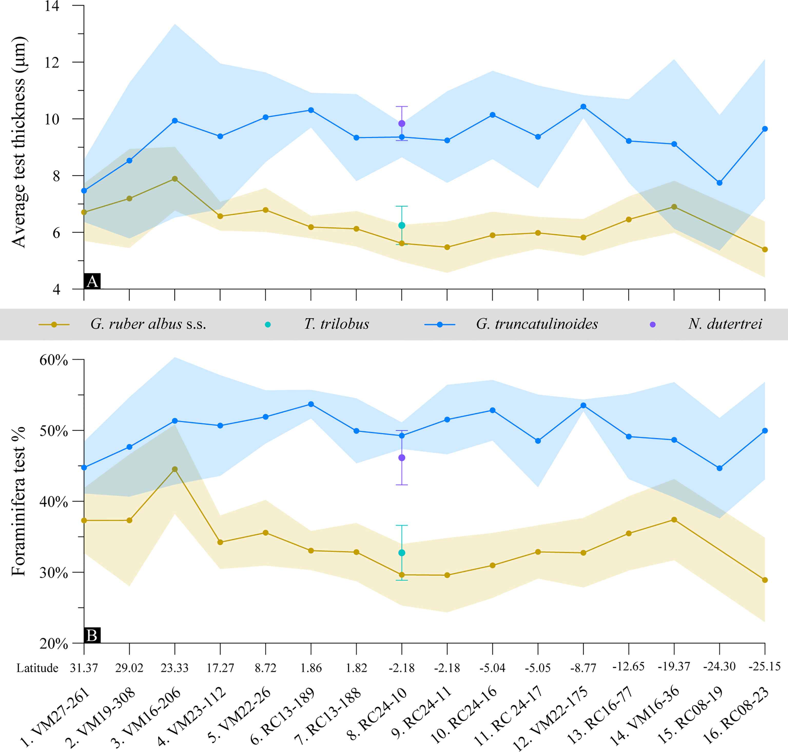
Figure 8 (A) Average thickness of the XMCT scanned foraminifera tests along the study transect; (B) species-specific average calcite test volume percentage in the total foraminifera cell. The shaded areas depict the 1σ confidence interval in measurements.

Test thicknesses of the surface and deep dwelling species appear to overlap at the subtropical gyres, while the signal disentangles at the tropical areas where G. ruber albus starts thinning. Test properties overlapping may be related to habitat compression at the downwelling gyre regions. G. ruber albus tests become up to 46% thinner at the equatorial sites and this is also reflected in the solid test percentage within its cell. G. truncatulinoides shows no distinct trend along the transect but its test thickness variability is higher at the gyres that may be the result of a mixture of crusted and non-crusted individuals. We note that for the equatorial samples 6 (RC13-189) to 12 (VM22-175) where G. truncatulinoides test thickness shows the least variability the weighed specimens were counted to be 100% dextral (Supplementary Figure 3). The better test thickness consistency in this region may indicate non-encrusted G. truncatulinoides specimens. However, although test thickness variability may be distinct between the two species, the variability in test secretion is almost the same for both species (avg. 3-4%; Figure 8B).

The spatial XMCT data may also indirectly offer information on carbonate “rain ratio” (Archer and Maier-Reimer, 1994) changes in the central Atlantic surface waters from volume measurements of the internal shell space that are meant to accommodate the protoplasm. Protoplasm space for G. ruber albus and G. truncatulinoides were calculated by subtracting the calcite test volume from the total cell volume and the results are given in Table 2 together with the amount of (sediment) contamination segmented for each sample. It appears that most (66%) of G. ruber albus cell space may be filled with protoplasm, while for G. truncatulinoides this space is reduced to 52%, so the deep dwelling globorotalid cell is almost half calcite and half biomass. Although the “rain ratio” decreases towards the equator from a surface-dweller perspective, a generalization to population level is not supported by heavier calcified deeper dwelling species (Figure 8A). Lastly, G. truncatulinoides cells are on average 12% larger than that of G. ruber but they can accommodate 12% less protoplasm (Table 2).

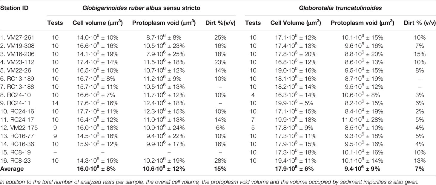
Table 2 Table of volumetric data from the spatial analysis of the tomographic images of the two different scanned species.

The cells of G. ruber albus become more voluminous at low latitude (Figure 8A) and since their tests are also thinner in this region (Supplementary Figure 4) the protoplasm voids are increased by ~20% in the south equatorial sites. Although the trend is not clear, almost the opposite is true for G. truncatulinoides for which the protoplasm voids are ~18% larger at the gyres than in most equatorial sites. There is also no clear trend for the total G. truncatulinoides cell volume along the transect. Thus overall G. ruber albus thickness and weight decrease as the protoplasm voids increase, while for G. truncatulinoides this is true only partly for its shell thickness (Supplementary Figure 4). The above suggests that surface plankton in the Atlantic equatorial upwelling regions have the potential to produce more organic to inorganic carbon compared to higher latitudes and that the overall efficiency may also be related to the faunal composition.

Contamination of specimens with sediment infill varies both between species and samples (Table 2). G. ruber specimens are infilled on average by 15% with detritus material and most contaminated are tests from the subtropical sediments. G. truncatulinoides tests however are far less contaminated (7%), possibly due to their smaller apertural openings. The degree of contamination of the G. ruber albus tests seems to have affected the shell weight measurements, since ~50% (R² = 0.53) of the shell weight variation may be explained by contamination. However, the good correlation between its test XMCT thickness and the independent shell weight measurements (R² = 0.63) restores credibility to the reported shell weight trends of G. ruber albus.

4 Discussion

4.1 Preservation and Integrity of the Calcareous Microfossils

The carbonate preservation of the studied samples was mainly assessed by XMCT scanning of two different planktonic foraminifera species of different solubility ranking. G. ruber albus is known as one of the most susceptible species of planktonic foraminifera to dissolution, while G. truncatulinoides is amongst the species most resistant to dissolution (Berger, 1968; Parker and Berger, 1971; Thunell and Honjo, 1981). In accordance with previous studies (Hertzberg and Schmidt, 2013), G. ruber albus specimens were found to be well preserved in most of the core locations with some signs of dissolution at the sites below the equatorial upwelling. The sample for which the highest dissolution was inferred from the CT analysis also showed deviation from the expected shell bulk densities. This deviation was translated to a ~14% G. ruber calcite loss to dissolution at this location and this is assumed to be the highest amount of dissolution in our samples. In line with the dissolution susceptibility ranking of these species (Berger, 1968; Petró et al., 2018), G. truncatulinoides tests were found consistently well preserved along the transect (Figure 7B). Consequently, we interpret the overall variation in foraminifera shell weights along the transect to reflect mainly a biotic response, rather than changes of dissolution states.

The X-ray analyses were performed on tests of planktonic foraminifera species that are known to have different dissolution susceptibilities. The difference in their susceptibility is most probably a result of the mineralogical composition of the tests rather than their morphological characteristics (Petró et al., 2018). Their preservation potential is most probably related to known Mg-banded lamellar calcite layering (Johnstone et al., 2011) as the different species display large variations in the Mg/Ca composition of individual tests. The pattern of Mg/Ca variation is notably different between symbiont-bearing and symbiont-free species. In symbiotic species like G. ruber, a cyclic Mg/Ca compositional banding occurs intercalated between broader low Mg/Ca bands (Fehrenbacher et al., 2017), while symbiont-free species, such as G. truncatulinoides, typically have fewer and broader compositional bands that may reflect more closely changes in calcification temperature as they migrate within the water column (Sadekov et al., 2005). This change in calcite mineralogy/purity can be traced in the CT number histograms of the different species as a shift in the distribution of the voxels within the high X-ray attenuation area towards higher CT numbers in the lower Mg-calcite of the deeper dwelling G. truncatulinoides (Figure 9).

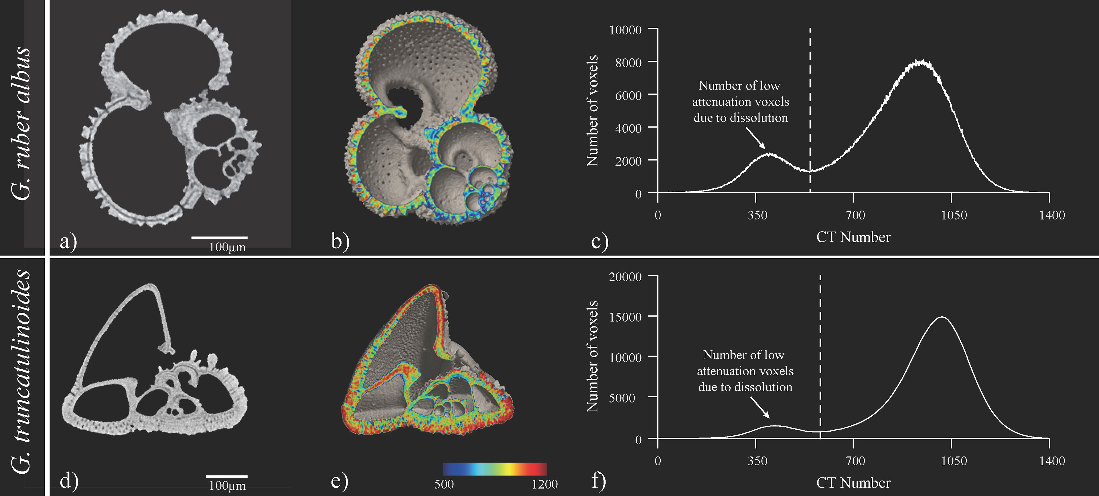
Figure 9 Illustration of XMCT data from site 9 (RC24-11). (A) is a tomographic image, (B) a cross-sectional isosurface image from CT image analysis software and (C) the CT number histogram of G. ruber albus and for G. truncatulinoides respectively characteristic (D) tomographic image, (E) cross-sectional isosurface image from CT image analysis software and (F) the CT number histogram. In (A) dissolution (higher Mg-calcite) is evident in the penultimate chamber as a grey gap in the middle of the shell wall but juvenile cambers are retained. In (D) similar grey gaps are present in the smaller chambers that are secreted in warmer waters can be observed for G. truncatulinoides as well. The mild bimodality of (C) at the low attenuation region of the histogram denote only minor dissolution.

Instead of the mean CT number, which as explained above might primarily reflect foraminifera test relative density, the ratio of the low attenuation voxels to the total test voxels was used in the present study as a dissolution index (CTX). Larger areas of low X-ray attenuation were found in the G. ruber albus specimens from the equatorial samples that are under the influence of the equatorial upwelling (Figure 9C). The increased dissolution of these samples may partly be related to the enhanced productivity of the region, which results in supralysoclinal dissolution (Archer et al., 1989) due to greater export and the subsequent degradation of organic matter at the sediment-water interface but also due to the thickness of the specimens, which gradually decreases towards the equatorial sites (Figure 8A). Thus, although the water temperature at the upwelling areas (Figure 3) does not suggest great mineralogical differences to justify enhanced test dissolution, yet the thinning of the tests from the enhanced upwelling area along the western African margin make them most susceptible to dissolution and breakage (see section 3.5). In contrast to G. ruber, the XMCT analyses of G. truncatulinoides tests showed good preservation. The CTX estimates were stable for all the samples and showed that the low attenuation calcite areas (corroded areas) are less than 7% of the total voxels. This signifies that the preservation of the biogenic carbonate material of the studied samples was good and that changes in shell weights are a result of biotic forcing. Overall, although the shells were found to be best preserved below the subtropical gyres, the overall preservation of the scanned specimens was found to be good. This is also manifested by the mild bimodality of the CT number histograms (Iwasaki et al., 2015; Iwasaki et al., 2019) from samples where the highest CTX was recorded (Figures 9C, D).

Dissolution primarily affects foraminifera test integrity rather than its outer geometry. It initially takes place at the more soluble phases of CaCO₃ such as the higher magnesium calcite layers of the test wall or as it progresses, at the juvenile chambers that are secreted in the warmer surface waters. The pattern of shell material loss within the chamber and intact outer and inner walls has been previously described (Johnstone et al., 2010) and although with progressing dissolution the relative test density decreases, the thickness and size of the shell remains intact (Ofstad et al., 2021). Hence, the reported variations in species test thickness (Figure 8A) are not a signal of dissolution but mainly reflect some biotic architectural response. There is however some concern whether the XMCT derived thicknesses indicate true shell thinning or an increase in shell porosity. Foraminifera shell porosity is known to increase towards the equator (Frerichs et al., 1972) and the gradual G. ruber thinning inferred by the XMCT analysis can also be explained by increased shell porosities. On the other hand, Weinkauf et al. (2020) suggested that a change in porosity should only have a negligible effect on shell weight and thus the lighter G. ruber shells found at the equator may indeed be the result of shell thinning as the XMCT suggests.

4.2 Shell Weight Variations

The planktonic foraminifera shells along the studied transect were found to be lighter in the equatorial regions. When averaged together the shell weights of the 8 studied species decrease by ~32% from an average of 21.5 μg in the subtropical gyres to 16.3 μg in the southern equatorial site (Table 1). The average foraminifera weights were found to be ~7.5% higher in the northern hemisphere samples, in line with previous observations for G. ruber (Hertzberg and Schmidt, 2013). The reason for this difference might be both the higher salinity (or density) of N. Atlantic subtropical waters (Figure 3). G. truncatulinoides tests were found to be ~3% lighter in the region where the sample consisted of 100% dextral specimens (samples 6. RC13-189 to 12. VM22-175). This is in line with the observations of Feldmeijer et al. (2015) that dextral specimens were found to calcify shallower and would thus require lighter tests. On the other hand, G. truncatulinoides showed high test calcification and thickness variability especially in the extra-equatorial region (Figure 8) perhaps due to a larger number of encrusted specimens, which is accordance with a more scattered, within the water column, growth/calcifying model that this species follows in the subtropics (Mulitza et al., 1997; LeGrande et al., 2004).

Since for all of the locations bottom water $\text{Δ}{\text{CO}}_3^{2-}$ did not vary considerably and the X-ray analyses did not suggest any severe shell dissolution, this collectively indicates that there is likely another factor controlling the weight differences between sites. When comparing with sea surface data, this shell weight variation in the study area was found also not to be related to surface water carbonate ion concentrations or to the degree of fragmentation but showed some moderate correlation to surface ocean density and salinity (section 3.2 and Supplementary Figure 1). The geochemistry of G. ruber shells from these samples was linked to surface ocean conditions (Arbuszewski et al., 2010). Since from the 8 weighed species only N. dutertrei and G. truncatulinoides occupy depths at or below the thermocline (Cléroux et al., 2007; Rebotim et al., 2019) averaged values are skewed towards the shallow-dwelling species. This might explain and validate associations with surface ocean properties.

However, when averaging the oceanographic parameters for the top 100 m, mean population shell weights reveal a relatively strong correlation with seawater salinity, while some dependency with ${\text{CO}}_3^{2-}$ and alkalinity also became apparent (Supplementary Figure 2). Salinity has previously been called upon to explain changes in planktonic foraminifera shell weight (Weinkauf et al., 2013), which might be linked to the concentration of ingredients required in shell formation. The seawater undergoes alkalization in internal foraminifera vacuoles by active ion pumping that elevates ${\text{CO}}_3^{2-}$ concentration and enhances calcification (Bentov et al., 2009; de Nooijer et al., 2009; Evans et al., 2018). Saltier, more alkaline ambient waters may have increased calcifying potential by reducing the energy requirements for ion transfer and promote foraminifera calcification or optimum shell growth. Notably any relation of shell weights to seawater density disappeared due to the complete elimination of the weight correlation with temperature (Supplementary Figure 2). Since temperature in known to affect planktonic foraminifera calcification and thus their shell weights (Qin et al., 2020; Titelboim et al., 2021), the absence of any correlation with temperature might be an artifact of averaging. This might be because both horizontal and vertical temperature and salinity gradients do not change to the same extent and salinity dominates in setting seasonal stratification in the tropics (Johnson et al., 2012). Besides salinity, temperature, [${\text{CO}}_3^{2-}$], optimum growth conditions and nutrient availability have been reported to affect foraminifera shell weights (de Villiers, 2004). If this was the case, then shell weights would have been higher in the warm and nutrient rich equatorial region, but this is not supported by the observations. In fact, shells are found to grow heavier within the oligotrophic subtropical gyres.

Although it is shown that shell weights generally increase according to the position of the foraminifera in the water column (Figure 4) there appears to be an inconsistency between the exact habitat depth known for each species and its sieve-based shell weights. That is because sieve-based shell weights are not normalized to their cell volumes and although size fraction is much constrained, it is still enough to allow for species-specific differences in size/volume. Within surface dwelling species this is evident for the different G. ruber chromotypes and the pink one although it is described to live shallower it is found heavier. This discrepancy is balanced out by the size of the specimens since the pink variety is larger than the white one (Hecht, 1976). The same is true for N. dutertrei and G. truncatulinoides (see section 3.5). However, G. aequilateralis appears to be an exception with anomalously light shells for its known habitat, which on the other hand shows how well protists can control their calcification.

Previous studies in the area confirm subsurface calcification depths for T. trilobus while O. universa is thought to have greater (Anand et al., 2003; Steph et al., 2009) or wider calcification depths (Farmer et al., 2007) in comparison to G. ruber. The apparently low shell weights of O. universa may stem from the fact that its final spherical chamber is not in geometric succession to the previous ones. Within the final calcification step O. universa changes its size abruptly and thus specimens that are found in a specific sieve fraction may be of a younger ontogenic stage (lower number of chambers) compared to the rest of the species that progress geometrically. A similar discrepancy exists for N. dutertrei that is found to have heavier shells than G. truncatulinoides, which is known to live deeper in the water column (Anand et al., 2003; Cléroux et al., 2013; Rebotim et al., 2016; Lessa et al., 2019). However, the XCMT analysis (see below) revealed that G. truncatulinoides is smaller in volume than N. dutertrei, which is found to be larger and thus its shell calcite is more sparsely distributed in space resulting in lower shell bulk densities ρ_shell (Figure 5).

G. ruber albus weight values however may to some extent be compromised both by dissolution and detrital sediment contamination. On average G. ruber specimens’ detrital contaminants occupy 14% of the internal void space, while contamination is highly variable (43%). Since at the time the present weight analysis was performed the samples were only treated with water (Arbuszewski et al., 2010; Hertzberg and Schmidt, 2013), the degree of decontamination is similar to that described in previous studies (Zarkogiannis et al., 2020c) for treatment only with deionized water prior to wet sieving. The above suggests that for studies of sediment samples, unless an effective cleaning method is used, the reported results of foraminifera shell weights, especially of species with large or multiple apertural openings, may be compromised by contamination. G. truncatulinoides shells on the other hand were far less contaminated and their weights did not appear to be influenced by the degree of their contamination. Furthermore, the shell weight values were not related to their preservation state, while bulk shell densities (i.e., volume normalized shell weights) showed no correlation with dissolution as well. Consequently, since dissolution has not affected all specimens, the consistent decrease in planktonic foraminifera shell weights at lower latitudes may be interpreted to reflect a biotic response.

Planktonic foraminifera shell weight variations are traditionally thought to reflect changes in the water column or sea floor [${\text{CO}}_3^{2-}$] (Lohmann, 1995; Barker and Elderfield, 2002; Osborne et al., 2016) but there is further evidence that this is not always the case. For example, at the same seawater [${\text{CO}}_3^{2-}$], foraminifera from different oceans have different shell weights, being heavier in the denser Atlantic (Broecker and Clark, 2001). Furthermore, both during the Pliocene (Davis et al., 2013) and the late Quaternary (Zarkogiannis et al., 2020b) the shell weights of planktonic foraminifera underneath the Intertropical Convergence Zone (ITCZ) were found to be invariant to atmospheric pCO₂ concentrations and thus changes in surface ocean [${\text{CO}}_3^{2-}$]. Zarkogiannis et al. (2019b) showed that glacial/interglacial shell weight changes vary with latitude and that the differences are greater at latitudes where the hydrology is sensitive to insolation gradients (Zarkogiannis et al., 2020b). Although moderate, the statistical correlation suggests that the observed foraminifera weight loss through shell expansion and thinning towards the equator may be the result of decreased water salinity and/or density. Tropical surface waters are relatively fresh due to excess rainfall associated with the convergent, ascending limbs of the Hadley circulation (ITCZ), whereas the subtropical oceans north and south of the equator are much saltier due to excess evaporation from the dry, descending limbs of the mean Hadley circulation. As a consequence, in these low latitude warmer and diluted waters, planktonic foraminifera would need to be lightly calcified to reach the ocean surface.

Changes in foraminifera calcite secretion according to ambient seawater densities has been previously proposed as a buoyancy regulation mechanism (Emiliani, 1954; Zarkogiannis et al., 2019a) so that foraminifera modify the mass of their shell accordingly to provide the “ballast” required for effective sinking at species specific depths (Marszalek, 1982). This is further demonstrated by the results of the present study, which show that shell weight is indeed a function of foraminifera position in the water column, and it increases with increasing depth habitat. Thus, despite the increase in acidity (Figure 1E) or the decrease in the degree of CaCO₃ saturation ($\text{Δ}{\text{CO}}_3^{2-}$) with depth (Figure 1D), foraminifera calcite secretion increases, such that surface dwelling foraminifera shells are lighter than their deeper dwelling counterparts. The fact that foraminifera shell mass increases with depth is also manifested by the heavily calcified shells of the benthic forms (Davis et al., 2016) that calcify on the sea floor where waters can be undersaturated with respect to CaCO₃. The results suggest that the degree of calcification may provide foraminifera a mechanism to control vertical movement or positioning in the water column irrespective of the CaCO₃ saturation state of the ambient water by actively modifying it by alkalization in internal vacuoles through ion pumping (Bentov et al., 2009; de Nooijer et al., 2009; Evans et al., 2018; Gagnon et al., 2021). Optimum shell growth in dictated by habitat density requirements and it is aided by seawater salinity.

A control of ambient seawater densities on foraminifera tests and a mechanism of active calcite secretion for habitat acquisition and maintenance may perhaps explain some known foraminifera characteristics such as the gametogenic calcite, pustules at their wall texture, and the change in compositional banding within the calcite walls. Foraminifera tend to increase their lipid content prior to gametogenesis to furnish their offspring (Bé et al., 1983). An increase in the lipid content would give positive buoyancy to the cell and will displace the organism to shallower depths. Gametogenic calcite may function to offset the lipid deposition in the gametes. On the other hand, calcite pustules that are found on the shell surface of deep dwelling species (Hemleben, 1975) may serve for habitat fine tuning in depths close or below the pycnocline. At these depths small changes in seawater density render large changes in depth and small calcite depositions in the form of pustules may provide the necessary weight. Furthermore, some species undergo daily vertical migrations, rising to the surface at darkness and descending to greater depths during the day (Holmes, 1982). The temperature decrease during the periods of darkness may be enough to increase the medium’s density and force foraminifera towards the surface and thus to still warmer waters. If not biologically mediated, this may explain the higher magnesium calcite lamellae that are secreted during the night (Fehrenbacher et al., 2017) and cannot be justified by the drop in the diurnal temperatures that takes place at least up to the base of the mixed layer (Gille, 2012). Wall banding in foraminifera reduces at depths (Sadekov et al., 2005) where temperatures are more stable.

4.3 Foraminifera Shell Bulk Densities

Foraminifera shell weight normalization to shell size is achieved with different methods that use either a linear dimension for normalization like measurement-based weights (Barker and Elderfield, 2002) and size-normalized weight (Beer et al., 2010) or methods that use two-dimensional approaches like area normalized shell weight (Osborne et al., 2016) and shell area density (Marshall et al., 2013) as approximations to a normalization against cell volume (Figure 2B). From the above methods the ones that use a liner measure although less accurate produce results that are still expressed in micrograms and are thus easily comparable between studies. On the other hand, the result of two-dimensional normalization is in μg/cm², which is thus less intuitive and not comparable to most studies. Ideally, weight would be normalized to the mean foraminifera cell volume, but cell volume has been more difficult and time consuming to establish. In the present study we used high resolution XMCT to accurately measure total foraminifera volumes and attempted a three-dimensional normalization of shell weights that led to the determination of foraminifera shell bulk densities.

Determination of non-motile plankton bulk densities is particularly important in the marine realm since they are driving the organismal positioning in the water column. It was only after the normalization over cell volume that foraminifera shell weights agreed with the preferable depth habitat for each species (Figure 5). This transformation revealed some further physiological characteristics of the different foraminifera species. From the scanned species of the 300-355 μm sieve fraction, surface dwelling G. ruber albus had the smallest and thinnest shells. T. trilobus that had (+10%) thicker test and was considerably heavier than G. ruber (~40%), manages to buoy at almost the same depths (Farmer et al., 2007) or usually only slightly deeper (Steph et al., 2009; Venancio et al., 2017) because its test is bigger and thus (+23%) more voluminous. Another such example is N. dutertrei, the test of which was found to be the heaviest of the analyzed species, yet it manages to live shallower in the water column than G. truncatulinoides (Cléroux et al., 2013), which produces the second heaviest tests (Figure 4). This is because although heavier, N. dutertrei is 13% bigger and so its shell bulk density is 13% lower than that of G. truncatulinoides.

The spatial information that resulted from the XMCT analyses allowed the determination of the size and percentage of the test within the cell of the scanned species. G. ruber albus has the smallest test but its average size increases towards the equator (Table 2), while its mean thickness decreases (Figure 8). Since its test does not simply become thinner by retaining the same size but also grows larger in the diluted equatorial waters, this suggests that as G. ruber approaches a thickness limit it may adjust its buoyancy by scaling its volume to match ambient seawater densities and meet certain depths. Accordingly, changes in test size may to some extent be physiological adaptations for buoyancy regulation. However, this is not entirely clear for G. truncatulinoides, which although it reaches its larger volumes in the tropics, in two of the equatorial samples, sizes decrease. Thus, size changes as a buoyancy regulation mechanism may apply mostly to surface dwelling species that encounter the lowest and most variable seawater densities. We interpret variations in test size and thickness to reflect a physiological response, rather than dissolution states, since dissolution lowers the test relative density (Figure 2D) but it leaves the thickness and the size of the test intact (Johnstone et al., 2010; Ofstad et al., 2021).

The XMCT analyses of the specimens showed that the lowest concentrations of solid material within the foraminifera cell is 30% and it is found in G. ruber albus primarily at the equatorial sites. On average the test of the G. ruber occupies 34% of its total (cell) volume and these values characterize tropical waters. These percentages are lower than those reported for similar sized specimens by Todd et al. (2020) from the Caribbean during the late Pliocene. Since late Pliocene atmospheric pCO₂ concentrations are comparable to today (Seki et al., 2010; Martínez-Botí et al., 2015) and global temperatures 2 to 3°C warmer (Haywood et al., 2016), higher pelagic calcification may be the result of the influence of the intense, warm and saltier (~1 kg/m³ denser) Mediterranean outflow to the Atlantic during the late Pliocene that altered the N. Atlantic oceanography (Khélifi et al., 2009). Along the transect, the solid test fraction of G. ruber albus varies by 55%, while for other globigerinids in the Atlantic the test fraction was found to vary up to 110% across the last glacial maximum (Zarkogiannis, 2021). This enhanced plasticity of the extent of sea surface plankton shell precipitation may be an important factor in regulating atmospheric CO₂ over the geologic time, since the production of biogenic CaCO₃ affects the alkalinity of seawater and thus the capacity of the ocean to absorb CO₂ from the atmosphere (Zondervan et al., 2001).

The deep dwelling G. truncatulinoides is more heavily calcified and test percentage varies only 27% along the transect. On average its test accounts for 47% of the total cell volume, while the maximum sample-averaged test percentage was recorded to be 52%. This small calcification variability implies that G. truncatulinoides has a better control on its calcification. If this narrow calcification window was the result of environmental and habitat stability, then calcification depth reconstructions for this species would have been steady. However, adult shell geochemistry suggests large regional variation of its mean calcification depths along the transect (Cléroux et al., 2013). We interpret this consistency in the amount of calcification as reflecting precision in buoyancy control, since adult G. truncatulinoides along the transect were found to calcify at or below the permanent (Feucher et al., 2016) pycnocline (Cléroux et al., 2007; Cléroux et al., 2013). Within this part of the water column (compared to the surface, mixed layer) densities vary less with depth and over wide depth ranges seawater density differences (Δρ) are small. Hence, small changes in the calcification of species that inhabit these depths result in large shifts of neutral buoyancy depths (Eq. 5). Therefore, deep-dwelling species may afford only small changes in their shell bulk densities, if they are to maintain certain depth ranges.

The organism (protoplasm and skeleton) will be neutrally buoyant only if the protoplasm compensates for the weight of the skeleton and the protoplast can indeed achieve a specific gravity significantly less than that of the ambient sea water (see below). The above biomass and calcite volume estimates confirm the hypothesis of Emiliani (1954) that the most important factor for foraminifera to live at certain depths is the ratio of the mass of the protoplasm and inclusions to the mass of the test and that when species have the largest ratio (G. ruber albus) they will prefer shallow habitats, while species with a smaller ratio will occupy deeper habitats (such as G. truncatulinoides).

4.4 Foraminifera Intracellular Density

The subtraction of the seawater density at neutral buoyancy depth from the foraminifera shell bulk density allowed the determination of foraminifera intracellular density and are in agreement with previous theoretical calculations (Marszalek, 1982). Intracellular density, a cumulative measure of the concentrations of all cellular components, impacts the physical nature of the cytoplasm and can globally affect cellular processes (Odermatt et al., 2021), yet cytoplasmic density regulation of foraminifera remains poorly understood. Although intracellular densities were found to be less than water or surface seawater density for both the shallow and deep dwelling groups, they varied considerably both between and within species. The present approach showed that on average the cell of G. ruber albus may have intracellular densities similar to that of mammalian (Kim and Guck, 2020) or yeast (Odermatt et al., 2021) cells. However, reconstructed values vary greatly with the cytoplasm appearing very diluted in some equatorial samples. This uncertainty may be the result of some apparent positive buoyancy that drive foraminifera to calcify at depths shallower than that dictated by organismal density. For example, within the mixed layer, foraminiferal spines may help heavier organisms to harvest turbulence and upwelling flow velocities to ascend to shallower depths or decrease their settling velocity (Lipps, 1973; Takahashi and Be, 1984; Furbish and Arnold, 1997). In such environments ρ_cyt from Equation 4 may be underestimated. If we hypothesize that ρ_cyt does not vary much between the studied surface and deep dwelling species and we subtract ρ_cyt of G. truncatulinoides from ρ_shell then we come up with organismal densities lower than that of water, which cannot be true. Thus, we conclude that the cytoplasm of spinose foraminifera is lighter than that of the non-spinose species but cannot be constrained solely from Equation 4.

The intracellular density differences both within a group and between groups may partly be due to the high variability in the cellular carbon content (Michaels et al., 1995), osmolytes (Boyd and Gradmann, 2002) and the variability of the water content and the density (i.e. salinity) of the intracellular water. Although foraminifera may to some degree osmoregulate, through a narrow tubular channel system, which resembles the contractile vacuole that is documented to be involved in osmoregulation in other protists as well (Gerisch et al., 2002), in terms of energy efficiency, it is logical to assume that they are largely isotonic with ambient seawater. Isotonic conditions would require higher density cellular fluids in deep dwelling-species, and this may explain the increased intracellular density reconstructions for G. truncatulinoides. Furthermore, the intracellular density may also be a function of the state of the lipidome. The effect of increasing pressure on the structure of lipids and lipid assemblies is generally qualitatively similar to the effect of decreasing temperature (Brooks, 2014). Hence, at thermocline temperatures the lipids of these ectotherms rather than being fluid must be ordered in a densely compacted gel phase (Schneider et al., 1999), such that the aggregate density of the animal will become greater as well. However, the greater compressibility of lipids compared to seawater makes any depth of neutral buoyancy unstable (Campbell and Dower, 2003).

5 Conclusions

The weight of the shells of several planktonic foraminifera species from core-top samples were studied together with their meridional and bathymetric changes across the central Atlantic regions. For a given species, planktonic foraminifera shell weights show dependency to ambient salinities and to a lesser degree on [${\text{CO}}_3^{2-}$] and alkalinity in the upper water column. However, despite the decreasing calcite saturation state of the water column with depth, species specific shell weights were found to increase with depth as a function of their preferred depth habitat.

Although interspecies test size variations may not be controlled by the position of the species in the water column, intraspecies size changes of mixed layer foraminifera may take place for buoyancy regulation purposes. The studied fossils were found to be overall well preserved. Some preferential dissolution was observed, and it was found to be species and site specific. Consequently, changes in foraminifera sizes and weights were interpreted to reflect a biotic response to changes primarily in ambient seawater salinity, rather than a dissolution biased signal. Nonetheless, foraminifera shell weight measurements were vulnerable to the degree of test internal contamination with sedimentary residuals. Improved cleaning procedures are essential for fossil shell weight studies.

The calculation of shell bulk densities was a key feature of the present study and integrates previous attempts of planktonic foraminifera shell weight normalization. This study attempted to describe the physical properties of the planktonic foraminifera shells but additional species-specific comparisons between shell masses and the various oceanographic parameters are needed as future work.

Data Availability Statement

The high resolution microcomputed tomographic datasets generated and analysed for this study can be found in the FIGSHARE data repository at https://doi.org/10.6084/m9.figshare.17088860.v1 for G. ruber and at https://doi.org/10.6084/m9.figshare.19747198.v2 for G. truncatulinoides.

Author Contributions

Conceptualization, SZ; methodology and investigation, SZ; software, formal analysis, SZ, SI and JWBR; resources, MS and JH; writing—original draft preparation, SZ. writing—review and editing, RR, PM, JH, JWBR and GK; visualization, SZ, SI and JWBR. All authors listed, have made substantial, direct, and intellectual contribution to the work, and approved it for publication.

Funding

This research was supported in part by a Royal Society Newton International postdoctoral Fellowship to SZ from the Royal Society of London. JWBR acknowledges funding from the European Research Council under the European Union’s Horizon 2020 research and innovation program (grant agreement 805246). We also acknowledge support from U.K. NERC Grant (PUCCA) NE/V011049/1.

Conflict of Interest

The authors declare that the research was conducted in the absence of any commercial or financial relationships that could be construed as a potential conflict of interest.

Publisher’s Note

All claims expressed in this article are solely those of the authors and do not necessarily represent those of their affiliated organizations, or those of the publisher, the editors and the reviewers. Any product that may be evaluated in this article, or claim that may be made by its manufacturer, is not guaranteed or endorsed by the publisher.

Acknowledgments

The authors would like to thank Professor Wolfgang Kiessling for generously providing access to the X-ray microtomographic facility of the Geozentrum Nordbayern of Friedrich-Alexander-Universität Erlangen-Nürnberg. This research used samples provided by the Lamont-Doherty Core Repository.

Supplementary Material

The Supplementary Material for this article can be found online at: https://www.frontiersin.org/articles/10.3389/fmars.2022.864801/full#supplementary-material

References

Anand P., Elderfield H., Conte M. H. (2003). Calibration of Mg/Ca Thermometry in Planktonic Foraminifera From a Sediment Trap Time Series. Paleoceanography 18 (2), 1050–1065. doi: 10.1029/2002pa000846
Antonarakou A., Kontakiotis G., Mortyn P. G., Drinia H., Sprovieri M., Besiou E., et al. (2015). Biotic and Geochemical (δ18O, δ13c, Mg/Ca, Ba/Ca) Responses of Globigerinoides Ruber Morphotypes to Upper Water Column Variation During the Last Deglatiation, Gulf of Mexico. Geochim. Cosmochim. Acta 170, 69–93. doi: 10.1016/j.gca.2015.08.003
Araujo M., Limongi C., Servain J., Silva M., Leite F. S., Veleda D., et al. (2011). Salinity-Induced Mixed and Barrier Layers in the Southwestern Tropical Atlantic Ocean Off the Northeast of Brazil. Ocean. Sci. 7 (1), 63–73. doi: 10.5194/os-7-63-2011
Arbuszewski J., deMenocal P., Kaplan A., Farmer E. C. (2010). On the Fidelity of Shell-Derived δ18Oseawater Estimates. Earth Planet. Sci. Lett. 300 (3–4), 185–196. doi: 10.1016/j.epsl.2010.10.035
Archer D., Emerson S., Reimers C. (1989). Dissolution of Calcite in Deep-Sea Sediments: pH and O2 Microelectrode Results. Geochim. Cosmochim. Acta 53 (11), 2831–2845. doi: 10.1016/0016-7037(89)90161-0
Archer D., Maier-Reimer E. (1994). Effect of Deep-Sea Sedimentary Calcite Preservation on Atmospheric CO2 Concentration. Nature 367 (6460), 260–263. doi: 10.1038/367260a0
Aurahs R., Treis Y., Darling K., Kucera M. (2011). A Revised Taxonomic and Phylogenetic Concept for the Planktonic Foraminifer Species Globigerinoides Ruber Based on Molecular and Morphometric Evidence. Mar. Micropaleontol. 79 (1), 1–14. doi: 10.1016/j.marmicro.2010.12.001
Barker S., Elderfield H. (2002). Foraminiferal Calcification Response to Glacial-Interglacial Changes in Atmospheric CO2. Science 297 (5582), 833–836. doi: 10.1126/science.1072815
Barker S., Kiefer T., Elderfield H. (2004). Temporal Changes in North Atlantic Circulation Constrained by Planktonic Foraminiferal Shell Weights. Paleoceanography 19 (3), PA3008. doi: 10.1029/2004pa001004
Bé A. W. H., Anderson O. R., Faber W. W., Caron D. A. (1983). Sequence of Morphological and Cytoplasmic Changes During Gametogenesis in the Planktonic Foraminifer Globigerinoides Sacculifer (Brady). Micropaleontology 29 (3), 310–325. doi: 10.2307/1485737
Beer C. J., Schiebel R., Wilson P. A. (2010). Technical Note: On Methodologies for Determining the Size-Normalised Weight of Planktic Foraminifera. Biogeosciences 7 (7), 2193–2198. doi: 10.5194/bg-7-2193-2010
Bentov S., Brownlee C., Erez J. (2009). The Role of Seawater Endocytosis in the Biomineralization Process in Calcareous Foraminifera. Proc. Natl. Acad. Sci. 106 (51), 21500–21504. doi: 10.1073/pnas.0906636106
Berger W. H. (1968). Planktonic Foraminifera: Selective Solution and Paleoclimatic Interpretation. Deep. Sea. Res. Oceanog. Abst. 15 (1), 31–43. doi: 10.1016/0011-7471(68)90027-2
Boyd C., Gradmann D. (2002). Impact of Osmolytes on Buoyancy of Marine Phytoplankton. Mar. Biol. 141 (4), 605–618. doi: 10.1007/s00227-002-0872-z
Broecker W., Clark E. (2001). An Evaluation of Lohmann's Foraminifera Weight Dissolution Index. Paleoceanography 16 (5), 531–534. doi: 10.1029/2000pa000600
Brooks N. (2014). Pressure Effects on Lipids and Bio-Membrane Assemblies. IUCrJ 1 (6), 470–477. doi: 10.1107/S2052252514019551
Campbell R. W., Dower J. F. (2003). Role of Lipids in the Maintenance of Neutral Buoyancy by Zooplankton. Mar. Ecol. Prog. Ser. 263, 93–99. doi: 10.3354/meps263093
Cléroux C., Cortijo E., Duplessy J.-C., Zahn R. (2007). Deep-Dwelling Foraminifera as Thermocline Temperature Recorders. Geochem. Geophys. Geosys. 8 (4), 19. doi: 10.1029/2006GC001474
Cléroux C., deMenocal P., Arbuszewski J., Linsley B. (2013). Reconstructing the Upper Water Column Thermal Structure in the Atlantic Ocean. Paleoceanography 28 (3), 503–516. doi: 10.1002/palo.20050
Dai Y., Yu J., deMenocal P., Hyams-Kaphzan O. (2019). Influences of Temperature and Secondary Environmental Parameters on Planktonic Foraminiferal Mg/Ca: A New Core-Top Calibration. Geochem. Geophys. Geosys. 20, 4370–4381. doi: 10.1029/2019GC008526
Davis C. V., Badger M. P. S., Bown P. R., Schmidt D. N. (2013). The Response of Calcifying Plankton to Climate Change in the Pliocene. Biogeosciences 10 (9), 6131–6139. doi: 10.5194/bg-10-6131-2013
Davis C. V., Myhre S. E., Hill T. M. (2016). Benthic Foraminiferal Shell Weight: Deglacial Species-Specific Responses From the Santa Barbara Basin. Mar. Micropaleontol. 124, 45–53. doi: 10.1016/j.marmicro.2016.02.002
de Nooijer L. J., Toyofuku T., Kitazato H. (2009). Foraminifera Promote Calcification by Elevating Their Intracellular pH. Proc. Natl. Acad. Sci. 106 (36), 15374–15378. doi: 10.1073/pnas.0904306106
de Villiers S. (2004). Optimum Growth Conditions as Opposed to Calcite Saturation as a Control on the Calcification Rate and Shell-Weight of Marine Foraminifera. Mar. Biol. 144 (1), 45–49. doi: 10.1007/s00227-003-1183-8
Emiliani C. (1954). Depth Habitats of Some Species of Pelagic Foraminifera as Indicated by Oxygen Isotope Ratios. Am. J. Sci. 252 (3), 149–158. doi: 10.2475/ajs.252.3.149
Evans D., Müller W., Erez J. (2018). Assessing Foraminifera Biomineralisation Models Through Trace Element Data of Cultures Under Variable Seawater Chemistry. Geochim. Cosmochim. Acta 236, 198–217. doi: 10.1016/j.gca.2018.02.048
Farmer E. C., Kaplan A., de Menocal P. B., Lynch-Stieglitz J. (2007). Corroborating Ecological Depth Preferences of Planktonic Foraminifera in the Tropical Atlantic With the Stable Oxygen Isotope Ratios of Core Top Specimens. Paleoceanography 22 (3), 14. doi: 10.1029/2006PA001361
Fehrenbacher J. S., Russell A. D., Davis C. V., Gagnon A. C., Spero H. J., Cliff J. B., et al. (2017). Link Between Light-Triggered Mg-Banding and Chamber Formation in the Planktic Foraminifera Neogloboquadrina Dutertrei. Nat. Commun. 8, 15441. doi: 10.1038/ncomms15441
Feldmeijer W., Metcalfe B., Brummer G.-J. A., Ganssen G. M. (2015). Reconstructing the Depth of the Permanent Thermocline Through the Morphology and Geochemistry of the Deep Dwelling Planktonic Foraminifer Globorotalia Truncatulinoides. Paleoceanography 30 (1), 1–22. doi: 10.1002/2014PA002687
Feucher C., Maze G., Mercier H. (2016). Mean Structure of the North Atlantic Subtropical Permanent Pycnocline From In Situ Observations. J. Atmosph. Ocean. Technol. 33 (6), 1285–1308. doi: 10.1175/jtech-d-15-0192.1
Frerichs W. E., Heiman M. E., Borgman L. E., Be A. W. H. (1972). Latitudal Variations in Planktonic Foraminiferal Test Porosity: Part 1. Optical Studies. J. Foraminiferal. Res. 2 (1), 6–13. doi: 10.2113/gsjfr.2.1.6
Furbish J. D., Arnold A. J. (1997). Hydrodynamic Strategies in the Morphological Evolution of Spinose Planktonic Foraminifera. Geologic. Soc. America Bull. 109 (8), 1055–1072. doi: 10.1130/0016-7606(1997)109<1055:HSITME>2.3.CO;2
Gagnon A. C., Gothmann A. M., Branson O., Rae J. W. B., Stewart J. A. (2021). Controls on Boron Isotopes in a Cold-Water Coral and the Cost of Resilience to Ocean Acidification. Earth Planet. Sci. Lett. 554, 116662. doi: 10.1016/j.epsl.2020.116662
Gerisch G., Heuser J., Clarke M. (2002). Tubular-Vesicular Transformation in the Contractile Vacuole System of Dictyostelium. Cell Biol. Int. 26 (10), 845–852. doi: 10.1006/cbir.2002.0938
Gille S. T. (2012). Diurnal Variability of Upper Ocean Temperatures From Microwave Satellite Measurements and Argo Profiles. J. Geophys. Res.: Ocean0 117 (C11), 16. doi: 10.1029/2012JC007883
Haywood A. M., Dowsett H. J., Dolan A. M. (2016). Integrating Geological Archives and Climate Models for the Mid-Pliocene Warm Period. Nat. Commun. 7 (1), 10646. doi: 10.1038/ncomms10646
Hecht A. D. (1976). An Ecologic Model for Test Size Variation in Recent Planktonic Foraminifera: Applications to the Fossil Record. J. Foraminiferal. Res. 6 (4), 295–311. doi: 10.2113/gsjfr.6.4.295
Hemleben C. (1975). Spine and Pustule Relationships in Some Recent Planktonic Foraminifera. Micropaleontology 21 (3), 334–341. doi: 10.2307/1485199
Hemleben C., Anderson O. R., Spindler M. (1989). Modern Planktonic Foraminifera (New York: Springer-Verlag).
Hertzberg J. E., Schmidt M. W. (2013). Refining Globigerinoides Ruber Mg/Ca Paleothermometry in the Atlantic Ocean. Earth Planet. Sci. Lett. 383, 123–133. doi: 10.1016/j.epsl.2013.09.044
Hofmann G. E., Barry J. P., Edmunds P. J., Gates R. D., Hutchins D. A., Klinger T., et al. (2010). The Effect of Ocean Acidification on Calcifying Organisms in Marine Ecosystems: An Organism-To-Ecosystem Perspective. Annu. Rev. Ecol. Evol. Systemat. 41 (1), 127–147. doi: 10.1146/annurev.ecolsys.110308.120227
Holmes N. (1982). Diel Vertical Variations in Abundance of Some Planktonic Foraminifera From the Rockall Trough, Northeastern Atlantic Ocean. J. Foraminiferal. Res. 12 (2), 145–150. doi: 10.2113/gsjfr.12.2.145
Iwasaki S., Kimoto K., Okazaki Y., Ikehara M. (2019). Micro-CT Scanning of Tests of Three Planktic Foraminiferal Species to Clarify DissolutionProcess and Progress. Geochem. Geophys. Geosys. 20 (12), 6051–6065. doi: 10.1029/2019GC008456
Iwasaki S., Kimoto K., Sasaki O., Kano H., Honda M. C., Okazaki Y. (2015). Observation of the Dissolution Process of Globigerina Bulloides Tests (Planktic Foraminifera) by X-Ray Microcomputed Tomography. Paleoceanography 30 (4), 317–331. doi: 10.1002/2014PA002639
Johnson G. C., Schmidtko S., Lyman J. M. (2012). Relative Contributions of Temperature and Salinity to Seasonal Mixed Layer Density Changes and Horizontal Density Gradients. J. Geophys. Res.: Ocean0 117 (C4), 13. doi: 10.1029/2011JC007651
Johnstone H. J. H., Schulz M., Barker S., Elderfield H. (2010). Inside Story: An X-Ray Computed Tomography Method for Assessing Dissolution in the Tests of Planktonic Foraminifera. Mar. Micropaleontol. 77 (1), 58–70. doi: 10.1016/j.marmicro.2010.07.004
Johnstone H. J. H., Yu J., Elderfield H., Schulz M. (2011). Improving Temperature Estimates Derived From Mg/Ca of Planktonic Foraminifera Using X-Ray Computed Tomography–Based Dissolution Index, XDX. Paleoceanography 26 (1), 17. doi: 10.1029/2009PA001902
Key R. M., Kozyr A., Sabine C. L., Lee K., Wanninkhof R., Bullister J. L., et al. (2004). A Global Ocean Carbon Climatology: Results From Global Data Analysis Project (GLODAP). Global Biogeochem. Cycle. 18 (4), 23. doi: 10.1029/2004GB002247
Khélifi N., Sarnthein M., Andersen N., Blanz T., Frank M., Garbe-Schönberg D., et al. (2009). A Major and Long-Term Pliocene Intensification of the Mediterranean Outflow, 3.5–3.3 Ma Ago. Geology 37 (9), 811–814. doi: 10.1130/g30058a.1
Kim K., Guck J. (2020). The Relative Densities of Cytoplasm and Nuclear Compartments Are Robust Against Strong Perturbation. Biophys. J. 119 (10), 1946–1957. doi: 10.1016/j.bpj.2020.08.044
LeGrande A. N., Lynch-Stieglitz J., Farmer E. C. (2004). Oxygen Isotopic Composition of Globorotalia Truncatulinoides as a Proxy for Intermediate Depth Density. Paleoceanography 19 (4), PA4025. doi: 10.1029/2004pa001045
Lessa D., Morard R., Jonkers L., Venancio I. M., Reuter R., Baumeister A., et al. (2019). Vertical Distribution of Planktonic Foraminifera in the Subtropical South Atlantic: Depth Hierarchy of Controlling Factors. Biogeosci. Discuss. 2019, 1–29. doi: 10.5194/bg-2019-355
Lipps J. H. (1973). Test Structure in Foraminifera. Annu. Rev. Microbiol. 27 (1), 471–486. doi: 10.1146/annurev.mi.27.100173.002351
Lipps J. H. (1979). “Ecology and Paleoecology of Planktic Foraminifera,” in Foraminiferal Ecology and Paleoecology. Eds. Lipps J. H., Berger W. H., Buzas M. A., Douglas R. G., Ross C. A. (SEPM Society for Sedimentary Geolog:Tulsa, Oklahoma), 62–104.
Lohmann G. P. (1995). A Model for Variation in the Chemistry of Planktonic Foraminifera Due to Secondary Calcification and Selective Dissolution. Paleoceanography 10 (3), 445–457. doi: 10.1029/95PA00059
Marshall B. J., Thunell R. C., Henehan M. J., Astor Y., Wejnert K. E. (2013). Planktonic Foraminiferal Area Density as a Proxy for Carbonate Ion Concentration: A Calibration Study Using the Cariaco Basin Ocean Time Series. Paleoceanography 28 (2), 363–376. doi: 10.1002/palo.20034
Marszalek D. S. (1982). The Role of Heavy Skeletons in Vertical Movements of non-Motile Zooplankton. Mar. Behav. Physiol. 8 (4), 295–303. doi: 10.1080/10236248209387026
Martínez-Botí M. A., Foster G. L., Chalk T. B., Rohling E. J., Sexton P. F., Lunt D. J., et al. (2015). Plio-Pleistocene Climate Sensitivity Evaluated Using High-Resolution CO2 Records. Nature 518 (7537), 49–54. doi: 10.1038/nature14145
McClelland H. L. O., Barbarin N., Beaufort L., Hermoso M., Ferretti P., Greaves M., et al. (2016). Calcification Response of a Key Phytoplankton Family to Millennial-Scale Environmental Change. Sci. Rep. 6 (1), 34263. doi: 10.1038/srep34263
Meilland J., Siccha M., Kaffenberger M., Bijma J., Kucera M. (2021). Population Dynamics and Reproduction Strategies of Planktonic Foraminifera in the Open Ocean. Biogeosciences 18 (20), 5789–5809. doi: 10.5194/bg-18-5789-2021
Michaels A. F., Caron D. A., Swanberg N. R., Howse F. A., Michaels C. M. (1995). Planktonic Sarcodines (Acantharia, Radiolaria, Foraminifera) in Surface Waters Near Bermuda: Abundance, Biomass and Vertical Flux. J. Plankton. Res. 17 (1), 131–163. doi: 10.1093/plankt/17.1.131
Mortyn P. G., Charles C. D. (2003). Planktonic Foraminiferal Depth Habitat and δ18o Calibrations: Plankton Tow Results From the Atlantic Sector of the Southern Ocean. Paleoceanography 18 (2). doi: 10.1029/2001pa000637
Mulitza S., Durkoop A., Hale W., Wefer G., Stefan Niebler H. (1997). Planktonic Foraminifera as Recorders of Past Surface-Water Stratification. Geology 25 (4), 335–338. doi: 10.1130/0091-7613(1997)025<0335:PFAROP>2.3.CO;2
Odermatt P. D., Miettinen T. P., Lemière J., Kang J. H., Bostan E., Manalis S. R., et al. (2021). Variations of Intracellular Density During the Cell Cycle Arise From Tip-Growth Regulation in Fission Yeast. eLife 10, e64901. doi: 10.7554/eLife.64901
Ofstad S., Zamelczyk K., Kimoto K., Chierici M., Fransson A., Rasmussen T. L. (2021). Shell Density of Planktonic Foraminifera and Pteropod Species Limacina Helicina in the Barents Sea: Relation to Ontogeny and Water Chemistry. PLoS One 16 (4), e0249178. doi: 10.1371/journal.pone.0249178
Osborne E. B., Thunell R. C., Marshall B. J., Holm J. A., Tappa E. J., Benitez-Nelson C., et al. (2016). Calcification of the Planktonic Foraminifera Globigerina Bulloides and Carbonate Ion Concentration: Results From the Santa Barbara Basin. Paleoceanography 31 (8), 2016PA002933. doi: 10.1002/2016PA002933
Parker F. L., Berger W. H. (1971). Faunal and Solution Patterns of Planktonic Foraminifera in Surface Sediments of the South Pacific. Deep. Sea. Res. Oceanog. Abst. 18 (1), 73–107. doi: 10.1016/0011-7471(71)90017-9
Petró S. M., Pivel M. A. G., Coimbra J. C. (2018). Foraminiferal Solubility Rankings: A Contribution To the Search For Consensus. J. Foraminiferal. Res. 48 (4), 301–313. doi: 10.2113/gsjfr.48.4.301
Qin B., Li T., Xiong Z., Algeo T. J., Jia Q. (2020). Calcification of Planktonic Foraminifer Pulleniatina Obliquiloculata Controlled by Seawater Temperature Rather Than Ocean Acidification. Global Planet. Change 193, 103256. doi: 10.1016/j.gloplacha.2020.103256
Rebotim A., Voelker A. H. L., Jonkers L., Waniek J. J., Meggers H., Schiebel R., et al. (2016). Factors Controlling the Depth Habitat of Planktonic Foraminifera in the Subtropical Eastern North Atlantic. Biogeosci. Discuss. 2016, 1–48. doi: 10.5194/bg-2016-348
Rebotim A., Voelker A. H. L., Jonkers L., Waniek J. J., Schulz M., Kucera M. (2019). Calcification Depth of Deep-Dwelling Planktonic Foraminifera From the Eastern North Atlantic Constrained by Stable Oxygen Isotope Ratios of Shells From Stratified Plankton Tows. J. Micropalaeontol. 38 (2), 113–131. doi: 10.5194/jm-38-113-2019
Ridgwell A., Zeebe R. E. (2005). The Role of the Global Carbonate Cycle in the Regulation and Evolution of the Earth System. Earth Planet. Sci. Lett. 234 (3–4), 299–315. doi: 10.1016/j.epsl.2005.03.006
Sadekov A. Y., Eggins S. M., De Deckker P. (2005). Characterization of Mg/Ca Distributions in Planktonic Foraminifera Species by Electron Microprobe Mapping. Geochem. Geophys. Geosys. 6 (12), 14. doi: 10.1029/2005GC000973
Schiebel R. (2002). Planktic Foraminiferal Sedimentation and the Marine Calcite Budget. Global Biogeochem. Cycle. 16 (4), 1065. doi: 10.1029/2001gb001459
Schlitzer R. (2002). Interactive Analysis and Visualization of Geoscience Data With Ocean Data View. Comput. Geosci. 28 (10), 1211–1218. doi: 10.1016/S0098-3004(02)00040-7
Schneider M. F., Marsh D., Jahn W., Kloesgen B., Heimburg T. (1999). Network Formation of Lipid Membranes: Triggering Structural Transitions by Chain Melting. Proc. Natl. Acad. Sci. 96 (25), 14312–14317. doi: 10.1073/pnas.96.25.14312
Seki O., Foster G. L., Schmidt D. N., Mackensen A., Kawamura K., Pancost R. D. (2010). Alkenone and Boron-Based Pliocene Pco2 Records. Earth Planet. Sci. Lett. 292 (1), 201–211. doi: 10.1016/j.epsl.2010.01.037
Steinke S., Chiu H.-Y., Yu P.-S., Shen C.-C., Löwemark L., Mii H.-S., et al. (2005). Mg/Ca Ratios of Two Globigerinoides Ruber (White) Morphotypes: Implications for Reconstructing Past Tropical/Subtropical Surface Water Conditions. Geochem. Geophys. Geosys. 6 (11), 10. doi: 10.1029/2005gc000926
Steph S., Regenberg M., Tiedemann R., Mulitza S., Nürnberg D. (2009). Stable Isotopes of Planktonic Foraminifera From Tropical Atlantic/Caribbean Core-Tops: Implications for Reconstructing Upper Ocean Stratification. Mar. Micropaleontol. 71 (1-2), 1–19. doi: 10.1016/j.marmicro.2008.12.004
Sverdrup H. U., Johnson M. W., Fleming R. H. (1942). The Oceans: Their Physics, Chemistry, and General Biology (New York: Prentice-Hall, Inc).
Takahashi K., Be A. W. H. (1984). Planktonic Foraminifera: Factors Controlling Sinking Speeds. Deep. Sea. Res. Part A. Oceanog. Res. Pap. 31 (12), 1477–1500. doi: 10.1016/0198-0149(84)90083-9
Thunell R. C., Honjo S. (1981). Calcite Dissolution and the Modification of Planktonic Foraminiferal Assemblages. Mar. Micropaleontol. 6 (2), 169–182. doi: 10.1016/0377-8398(81)90004-9
Titelboim D., Lord O. T., Schmidt D. N. (2021). Thermal Stress Reduces Carbonate Production of Benthic Foraminifera and Changes the Material Properties of Their Shells. ICES. J. Mar. Sci. 78 (9), 3202–3211. doi: 10.1093/icesjms/fsab186
Todd C. L., Schmidt D. N., Robinson M. M., De Schepper S. (2020). Planktic Foraminiferal Test Size and Weight Response to the Late Pliocene Environment. Paleoceanog. Paleoclimatol. 35 (1), e2019PA003738. doi: 10.1029/2019PA003738
Toyofuku T., Matsuo M. Y., de Nooijer L. J., Nagai Y., Kawada S., Fujita K., et al. (2017). Proton Pumping Accompanies Calcification in Foraminifera. Nat. Commun. 8 (1), 14145. doi: 10.1038/ncomms14145
van Heuven S., Pierrot D., Rae J. W. B., Lewis E., Wallace D. W. R. (2011). “CO2SYS V 1.1,” in MATLAB Program Developed for CO2 System Calculations (Oak Ridge, Tennesee: Oak Ridge National Laboratory). ORNL/CDIAC-105b.
Venancio I. M., Belem A. L., Santos T. P., Lessa D. O., Albuquerque A. L. S., Mulitza S., et al. (2017). Calcification Depths of Planktonic Foraminifera From the Southwestern Atlantic Derived From Oxygen Isotope Analyses of Sediment Trap Material. Mar. Micropaleontol. 136, 37–50. doi: 10.1016/j.marmicro.2017.08.006
Weinkauf M. F. G., Moller T., Koch M. C., Kučera M. (2013). Calcification Intensity in Planktonic Foraminifera Reflects Ambient Conditions Irrespective of Environmental Stress. Biogeosciences 10 (10), 6639–6655. doi: 10.5194/bg-10-6639-2013
Weinkauf M. F. G., Zwick M. M., Kučera M. (2020). Constraining the Role of Shell Porosity in the Regulation of Shell Calcification Intensity in the Modern Planktonic Foraminifer Orbulina Universa D'orbigny. J. Foraminiferal. Res. 50 (2), 195–203. doi: 10.2113/gsjfr.50.2.195
Zarkogiannis S. D. (2021). Disruption of the Atlantic Meridional Circulation During Deglacial Climates Inferred From Planktonic Foraminiferal Shell Weights. J. Mar. Sci. Eng. 9 (5), 519. doi: 10.3390/jmse9050519
Zarkogiannis S. D., Antonarakou A., Fernandez V., Mortyn P. G., Kontakiotis G., Drinia H., et al. (2020b). Evidence of Stable Foraminifera Biomineralization During the Last Two Climate Cycles in the Tropical Atlantic Ocean. J. Mar. Sci. Eng. 8 (10), 737. doi: 10.3390/jmse8100737
Zarkogiannis S. D., Antonarakou A., Tripati A., Kontakiotis G., Mortyn P. G., Drinia H., et al. (2019a). Influence of Surface Ocean Density on Planktonic Foraminifera Calcification. Sci. Rep. 9 (1), 533. doi: 10.1038/s41598-018-36935-7
Zarkogiannis S., Fernandez V., Greaves M., Mortyn P. G., Kontakiotis G., Antonarakou A. (2020a). X-Ray Tomographic Data of Planktonic Foraminifera Species Globigerina Bulloides From the Eastern Tropical Atlantic Across Termination II. Gigabyte 1. doi: 10.46471/gigabyte.5
Zarkogiannis S. D., Kontakiotis G., Antonarakou A., Mortyn P. G., Drinia H. (2019b). Latitudinal Variation of Planktonic Foraminifera Shell Masses During Termination I. IOP. Conf. Series.: Earth Environ. Sci. 221, 12052. doi: 10.1088/1755-1315/221/1/012052
Zarkogiannis S. D., Kontakiotis G., Gkaniatsa G., Kuppili V. S. C., Marathe S., Wanelik K., et al. (2020c). An Improved Cleaning Protocol for Foraminiferal Calcite From Unconsolidated Core Sediments: HyPerCal—A New Practice for Micropaleontological and Paleoclimatic Proxies. J. Mar. Sci. Eng. 8 (12), 998. doi: 10.3390/jmse8120998
Zeebe R. E., Westbroek P. (2003). A Simple Model for the CaCO3 Saturation State of the Ocean: The 'Strangelove' the 'Neritan and the 'Cretan Ocean. Geochem. Geophys. Geosys. 4 (12), 1104. doi: 10.1029/2003gc000538
Keywords: planktonic foraminifera, shell weight, X-ray microtomography (µCT), shell bulk density, relative shell density, buoyancy regulation
Citation: Zarkogiannis SD, Iwasaki S, Rae JWB, Schmidt MW, Mortyn PG, Kontakiotis G, Hertzberg JE and Rickaby REM (2022) Calcification, Dissolution and Test Properties of Modern Planktonic Foraminifera From the Central Atlantic Ocean. Front. Mar. Sci. 9:864801. doi: 10.3389/fmars.2022.864801
Received: 28 January 2022; Accepted: 22 April 2022;
Published: 02 June 2022.
Edited by:
Jennifer Fehrenbacher, Oregon State University, United StatesReviewed by:
Jacek Raddatz, Goethe University Frankfurt, GermanyJeroen Groeneveld, University of Hamburg, Germany
Copyright © 2022 Zarkogiannis, Iwasaki, Rae, Schmidt, Mortyn, Kontakiotis, Hertzberg and Rickaby. This is an open-access article distributed under the terms of the Creative Commons Attribution License (CC BY). The use, distribution or reproduction in other forums is permitted, provided the original author(s) and the copyright owner(s) are credited and that the original publication in this journal is cited, in accordance with accepted academic practice. No use, distribution or reproduction is permitted which does not comply with these terms.
*Correspondence: Stergios D. Zarkogiannis, stergios.zarkogiannis@earth.ox.ac.uk