Lake Sediments Reveal Large Variations in Flood Frequency Over the Last 6,500 Years in South-Western Norway

Introduction

In October 2014, several villages and small cities in western Norway were hit by destructive floods [Davies, 2014; The Norwegian Water Resources Energy Directorate (NVE), 2020b]. Extreme precipitation over 3 days caused rivers to rise quickly above their average streamflow. The contribution from snowmelt was negligible, whereas glacier melt constituted a substantial contribution in (partially) glaciated catchments [The Norwegian Water Resources Energy Directorate (NVE), 2020a]. In the small city of Odda, the flood destroyed five houses and critical infrastructure, including roads and bridges (Dannevig et al., 2016). Odda was only one among numerous cities in western Norway that were hit by the flood in 2014 and again in 2015. The tendency of increased flooding due to changing climatic conditions has raised concern among many municipalities and at a federal governmental level (Alnes et al., 2018; Norwegian Climate Service Center, 2020).

Floods are a considerable problem in Norway, and the need for reliable predictions of floods and development of new adaptation strategies is urgent (Hanssen-Bauer et al., 2015; Lawrence, 2016). Estimates of recurrence intervals for floods, required for land-use planning and the design of critical infrastructure, are typically based on instrumental measurements. Only rarely are historical observations included in these estimates (Engeland et al., 2018a,b). However, as a rapidly changing climate exerts a growing influence on flood frequencies across Europe (Blöschl et al., 2017), one strategy that can potentially add insight into the flood–climate connection is to produce and explore geological records that document this relationship on centennial to millennial timescales. This alternative approach can allow for a better understanding of the full range of flood variability and how non-stationarity in floods could be linked to dynamic changes in climate (Støren et al., 2010; Stewart et al., 2011; Wilhelm et al., 2012; Wirth et al., 2013; Støren and Paasche, 2014). Over the past decade, several new studies have examined how changing flood regimes have left sedimentary imprints in downstream lakes (e.g., Wilhelm et al., 2018). Regardless of the length of the flood time series, the interplay between topoclimatic settings and local climate dynamics will govern and explain how floods play out during the year. Generally, intense snowmelt, torrential rain, or a mix of the two cause floods in Norway, although geographical variations are large (Lawrence, 2016). In the inland parts of eastern Norway, spring snowmelt is the main cause of floods (Roald, 2013). This is different from western Norway, where floods are the result of intense rains (Lawrence and Hisdal, 2011; Kobierska et al., 2018), often associated with atmospheric rivers causing landfalls (Hanssen-Bauer et al., 2015; Azad and Sorteberg, 2017; Whan et al., 2020). However, in small catchments, rain squalls are the dominating flood origin across the country. A third type of floods in Norway is Glacial Outburst Floods (GLOF) that origin from a glacial or moraine dammed lake that suddenly break and release large amounts of water [The Norwegian Water Resources Energy Directorate (NVE), 2020a]. A GLOF has the potential to transport large amount of sediments and to cause serious damage to nearby societies.

The westerly wind belt brings moist air to western Norway, especially during the winter months. High mountains, close to the coast of Norway, lead to an orographic enhanced precipitation that often involves intensified rain and snowfall on the windward side of the mountain chains that cross Norway in a south–north direction (Roald, 2008; Hanssen-Bauer et al., 2015). These factors make southwest Norway one of the regions with the highest annual rainfalls in Scandinavia. In addition to the polar-front pressure differences, remnants from tropical hurricanes and atmospheric rivers are known to cause large flooding events in this area (Roald, 2013). Since AD 1900, the average precipitation has increased by 18% in Norway, while the temperature has risen by 1°C [The Norwegian Water Resources Energy Directorate (NVE), 2017]. The increased temperature has resulted in earlier spring floods, and rain floods tend to be more frequent due to the increase in extreme precipitation (Hanssen-Bauer et al., 2015). In this context, a research question that is worth pursuing is as follows: Can valuable “climate analogs” from the past shed light on how unusual the present hydro-climatic situation is, and if so, can we indicate what to anticipate in the coming century?

In Norway, there are continuous flood reconstructions covering parts or the entire Holocene ( ≤ 11,700 years) from eastern Norway (Nesje et al., 2001; Bøe et al., 2006; Støren et al., 2010, 2012). Here, we present a 6,500 year-long sediment record from Sandvinvatnet, located at the head of the fjord Hardangerfjorden, south-western Norway. We use the sediment record to reconstruct flood frequencies over time, examine changes in the flood frequency, and investigate possible linkages to long-term changes in temperature and precipitation in the region.

Study Area—Lake Sandvinvatnet and the Buerdalen Valley

Lake Sandvinvatnet (4.3 km²) is located south of Odda in south-western Norway at the head of the fjord Hardangerfjorden (Figures 1A,B). The lake spans 5 km along the south-north axis and 1.5 km at its widest point. The maximum depth is about 130 m in the northern part, and there are steep mountainsides extending up to 1,600 m altitude surrounding the lake. The main inlet is at the southern end, and the outlet is through the river Opo through Odda. The lake is of glacial and tectonic origin and its original age is unknown. After the last glaciation, it was part of Hardangerfjorden being cut off, becoming a lake, around 9,500 years ago (Møller and Holmeslet, 2012). Historical records confirm that this area has experienced massive floods several times, with devastating consequences for houses, farms, infrastructure, people, and animals. The first well-documented flood in Opo and Sandvinvatnet happened on December 4th−5th, AD 1743, causing damage to farms and farmland along Hardangerfjorden (Kraftmuseet, 2019). Since then, there has been historical documentation of at least 15 extreme floods causing damage through the nineteenth and twentieth century (Roald, 2013; Kraftmuseet, 2019), with the latest large flood occurring in October 2017 (Varsom.no, 2017). Most of the floods in this area are caused by intense precipitation events combined with melting snow and ice in the mountains due to rapid warming after snowfall (Roald, 2013). Average annual precipitation is 1,800 mm and most rain usually fall in October (Climate-data.org, 2020). Floods occur from May to November, with a somewhat higher frequency in October (Figure 2). Snow and glacial melts often cause and/or contribute substantially to the floods in spring and summer, but most floods caused by snowmelt occur in combination with rain.

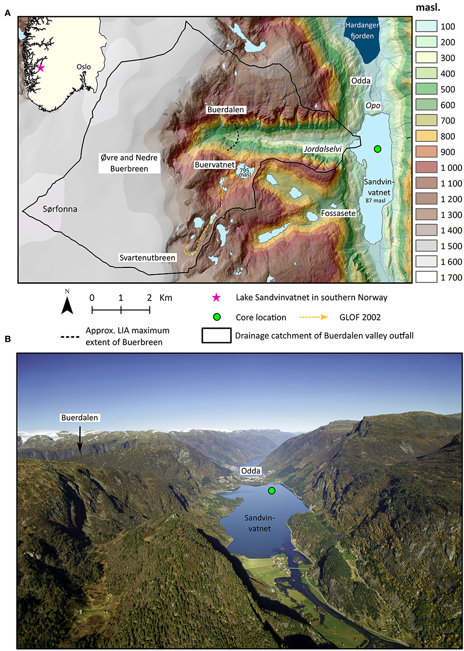
Figure 1. (A) Study site with Lake Sandvinvatnet (to the east) and the Buerdalen valley, Lake Buervatnet, and the Sørfonna icecap (Folgefonna) to the west (background image from Kartverket/norgeskart.no, 2020). The LIA maximum extent is marked for Øvre and Nedre Buerbreen (black dashed line; Bakke et al., 2000). Drainage catchment (black line) of the Buerdalen valley and the outlet glaciers at the head of the Jordalselvi stream [The Norwegian Water Resources Energy Directorate (NVE), 2020a]. The glacial outburst flood (GLOF) that occurred in 2002 went from a lake dammed at the outlet glacier Svartenutbreen to Lake Buervatnet (orange dashed line; Røthe et al., 2019). The inset shows southern Norway (©EuroGeographics for the administrative boundaries) and the pink star marks Sandvinvatnet's location. (B) Image of Lake Sandvinvatnet taken from the south direction (Photo: Jan Rabben). An image of Buerdalen valley can be seen in the Supplementary Material.

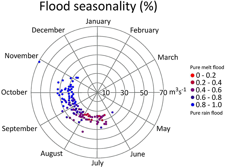
Figure 2. Diagram shows the independent flood peaks above 25 m³s⁻¹ since 1958 AD in the Buerdalen valley catchment and until 2018 AD (Figure 1). The relative contribution of snowmelt vs. rain for individual floods is shown as a color gradient going from red to blue, where red represents snowmelt-induced floods and blue denotes rain-induced floods. The percent values of the color scale are skewed. The radius indicates the magnitude of the floods (m³s⁻¹). All values are based on gridded SeNorge models for precipitation, temperature, snowmelt, and runoff (NVE et al., 2020) extracted for the Buerdalen valley catchment.

At the west side of Sandvinvatnet, there are two stream inlets, one major stream (Jordalselvi) draining the Buerdalen valley and a smaller stream draining Lake Fossasete, located on the plateau south of Jordalselvi (Figure 1A). Where Jordalselvi meets Sandvinvatnet, a delta has formed that is partly vegetated farmland. The total drainage area for Jordalselvi is about 52 km², with more than 50% of its catchment covered by the icecap Sørfonna [Figure 1A; The Norwegian Water Resources Energy Directorate (NVE), 2020a]. At the end of Buerdalen, two outlet glaciers from Sørfonna, named Øvre Buerbreen and Nedre Buerbreen, descend to the valley floor. Moraine ridges mark their “Little Ice Age” (LIA) maximum extent (Figure 1A). Along Jordalselvi, both fluvial and glaciofluvial material types have been observed [Bakke et al., 2000; Geological Survey of Norway (NGU), 2016]. Buerdalen is frequently subjected to landslides, rockfalls, and avalanches transporting sediments downslope, which makes them prone to remobilization by running water and floods. The many colluvial cones deposited in Buerdalen are evidence of this. From a glacier dammed lake near the outlet glacier Svartenutbreen (Figure 1A), there have been several GLOFs. There have been four historical GLOFs from 1910 to 2002 (Kjøllmoen, 2004; Jackson and Ragulina, 2014). Using lake sediments from Buervatnet (Figure 1A), Røthe et al. (2019) showed that 12 GLOFs occurred during the Holocene, providing a longer perspective on these rare forms of extremes and connecting their occurrence to the size of the glacier. During GLOFs, water gushes down to Buerdalen, following the path of Jordalselvi into Sandvinvatnet.

The bedrock around Buerbreen is granitic to amphibole bearing migmatite. Outside the LIA boundary (Figure 1A), monzogranite dominates, with some areas of granite [Geological Survey of Norway (NGU), 2020]. East of Sandvinvatnet, there is a plateau with steep vegetated bedrock slopes leading down to the lake. The bedrock on the eastern slopes is monzogranite, but quartz dominates the top of the plateau within bedrocks, such as quartzite, quartz schist, quartz mica schist, and quartz schistose [Geological Survey of Norway (NGU), 2020]. This part of the catchment falls within the Hardangervidda high mountain plateau and is drained by the river Storeelvi, which enters Sandvinvatnet in the southernmost part.

Methods and Materials

Lake Survey

The bathymetry of the lake was investigated using a Lowrance Elite 5 echo sounder and Edgtech 3100 chirp with a SB-424 (4–24 kHz) tow fish to find a flat lakebed surface suited for coring. The echo sounding profiles were interpolated to a bathymetry map using the “Nearest Neighbor” interpolation tool in the ArcGIS 10.5 software. The chirp profiles were visualized using SeiSee software.

Coring and Material

Two sediment cores were retrieved during two field seasons (2016 and 2017) from Sandvinvatnet using a 90 mm UWiTEC piston corer with a re-entry system (UWiTEC, 2020). The coring system retrieves sediments in 2 m sections, and the sediment core used in this study is a composite of two parallel cores (SA16 and SA17) taken with an overlap of approximately 1 m. Sediment core SA16 consists of four sections with lengths of 169, 171, 173, and 162 cm, whereas sediment core SA17 consists of four sections with lengths of 169, 166, 167, and 100 cm, respectively. The different core sections of SA16 and SA17 were combined to a composite core based on visual logs, surface photos, and magnetic susceptibility (MS) and cross-checked against the radiocarbon based chronology (see section Chronology) to create a complete sediment core (SA16/17). The combined sediment core has a total length of 830 cm. The uppermost soft sediments were retrieved using a UWiTEC gravity corer that preserves the sediment–water interface (sediment core named SAD616, 65 cm long; UWiTEC, 2020). All cores are from the same coring site (latitude 60.04195, longitude 6.55265) in the northern and deepest part (130 m) of Sandvinvatnet, where the lakebed is flat over a large area (Figure 3).

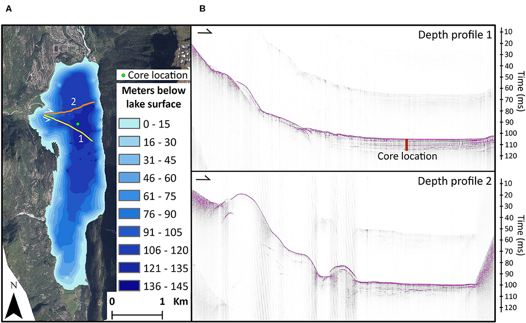
Figure 3. (A) Map over Sandvinvatnet and the bathymetry based on eco sounding measurements. The coring site is marked with a green dot. The orange and yellow lines show the location of the two seismic profiles shown in (B). (B) Two seismic profiles derived using a chirp starting at the delta front and ending close to the steep slope in the east. Profile 1 is close to the core location (indicated, not to scale, in depth profile 1). The depth at the coring site is close to 130 m.

Differentiating Magnetic Signatures and Identifying Flood Deposits in Lake Sediments

MS is a widely applied method for studying extreme events and glacial variability in lake sediments (e.g., Vasskog et al., 2011; Kvisvik et al., 2015; Røthe et al., 2019). It is a measure of a material's ability to acquire magnetization when exposed to a magnetic field. The different MS levels are referred to as diamagnetism (negative), paramagnetism (low), and ferro and ferrimagnetism (high; e.g., Thompson and Oldfield, 1986); they depend on the carriers in question, which typically consist of a mix of MS levels in natural samples.

MS was measured at 0.2 cm intervals at the split core surface using a GEOTEK Multi Sensor Core logger (Gunn and Best, 1998) with a Bartington MS2E point sensor. Distinct layers were identified by calculating the rate of change (ROC) of the MS values on the depth scale. Following Støren et al.'s (2010) approach, the hypothesis is that these rapid changes in MS mark the onset of individual flood layers as flood events are likely to increase the influx of minerogenic material to the lake. Thresholds of ROC exceeding the 95th and 97th percentiles were used to quantify the frequency of the most extreme changes in MS, and thus, the frequency of extreme flooding. Since some peaks in ROC of MS on sediment cores often consists of several values a second flood frequency analysis was produced only using the highest value of the ROC peaks as a comparison.

The hypothesis was further tested by measuring mass-specific MS (χbulk) on individual bulk samples through SA16/17 at 10 cm intervals (10 ml per sample) using a Multi-Function Kappa Bridge (MFK1-FA). Using χbulk makes it possible to check sediment samples for what kinds of magnetic carriers they possess. The samples were measured at two different temperatures, and the ratio was used for the analysis. This means that the MS values for a sample frozen with liquid nitrogen (77 K) should be 3.8 times higher than the MS values measured at room temperature (293 K) if the material is predominantly paramagnetic. Hence, a sample with a high ratio (around three) will be mostly paramagnetic, give a weak positive magnetic response and low MS values, e.g., NaCa₂(Mg, Fe, Al)₅(Al, Si)₈O₂₂(OH)₂ (amphibole). A sample with a low ratio (around one) will typically be ferromagnetic (or ferrimagnetic) and give a strong magnetic response and high MS values, e.g., Fe (Iron). Diamagnetic samples return negative MS values, e.g., SiO₂ (quartz), organic matter and water. In short, ferromagnetic dominating sediment samples will show higher MS values than pure paramagnetic sediment samples will (Walden et al., 1999). In mixed sediment deposits, the three magnetic mineral categories will often be present. Only a small portion of ferro and ferrimagnetic carriers can mask the presence of paramagnetic and diamagnetic minerals.

To ensure the full range of variability was obtained, the samples were supplemented with samples from 41 layers with extremely high MS values (above the 95th percentile of MS; hypothesized to represent floods), 5 samples from layers with intermediate MS values close to the MS trend line (Gaussian LOESS fit; representing background sediments), and 13 samples from layers with low MS values, such as centimeter-wide sand and clay layers in the core. The χbulk values were measured at room temperature (293 K) and 77 K. The ratio was calculated between χbulk_77K and χbulk_293K. SAD616 was subjected to eight χbulk measurements based on the chronology results (see section Chronology for details).

In environmental studies utilizing MS variations, the potentially varying influence of mineral concentration, mineral composition (which determines category of magnetism), crystal size, and crystal shape should be kept in mind and potentially tested given the initial scope of the study (Walden et al., 1999). The two latter factors signify that magnetic measurements may be influenced by the grain size of the sediments in the sample. To test whether physical grain size had an effect on MS and the χbulk measurements, we performed analysis on a selection of the same samples used for the χbulk measurement. The grain size analysis was carried out on 59 samples chosen to show the range of the MS dataset of SA16/17 described in the previous section and an additional 12 samples to cover the length of the core. The samples were first treated with 35% H₂O₂ to remove organic content (cf. Vasskog et al., 2016), then measured in a Malvern Mastersizer 3000 with an LV Hydro dispersion unit at a stirring speed of 2,500 rpm. Sample sizes were scaled to give obscuration values at 10–15%, the refraction index was set to 1.543, and a absorption index was used 0.01 as for quartz; all samples were measured three times at 20 s with red laser and 10 s with blue laser.

Chronology

Radiocarbon chronology is based upon 26 samples of macrofossils from both the sediment cores SA16 and SA17. All samples were analyzed at Poznan Radiocarbon Laboratory, Poland. The age–depth model was created using the R software package Bacon (Blaauw and Christen, 2011) with the IntCal13 calibration curve for calibration to calendar years before present.

The uppermost part of the SAD616 sediment core was sub-sampled at 1 cm intervals for the uppermost 50 cm. The samples were sent to the Department of Surface Waters Research and Management at the Swiss Federal Institute of Aquatic Science and Technology (Eawag), and the concentrations of 210-lead (²¹⁰Pb) and cesium (¹³⁷Cs) were analyzed and later used to construct an age–depth model for the uppermost part of the sediment core.

Results

Lake Bathymetry

The bathymetry of the lake showed the northern part of the lake to be the deepest, almost 130 m (Figure 3A). Two chirp profiles (Figure 3B) crossing the northern part of the lake from west to east revealed slopes from the delta from Buerdalen to the west and indicated steeper slopes to the east.

Core SA16/17

Figure 4 illustrates a plot of χbulk_293K vs. the ratio of χbulk_293K and χbulk_77K, where all samples fall along a log-linear regression line with a significant correlation coefficient of r² = 0.7 (p < 0.0001). This indicates ferromagnetic properties (low χbulk ratio) for samples with high MS values and paramagnetic properties (high χbulk ratio) for sediments with low MS values. All samples but one of the ROC of MS above the 95th percentile had a ratio lower than two (Figure 4B); this indicates that both high values and extreme changes in MS in SA16/17 are correlated with ferromagnetic properties.

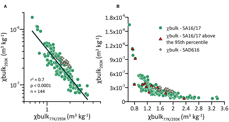
Figure 4. (A) χbulk_293K vs. χbulk_77K over χbulk_293K on a log scale. The strong correlation between the two variables suggests that the strength of magnetic susceptibility (MS) is related to the concentration of magnetic carriers. (B) The same plot as A, but on a regular scale. All χbulk samples are plotted. The samples identified above the 95th rate-of-change (ROC) percentile are represented by red triangles. Samples from SAD616 are shown as a pale yellow crosses. Both datasets plot along the SA16/17 dataset (green dots).

The sediment stratigraphy of core SA16/17 was divided into four facies with similar properties based on visual logging of the core and sediment surface MS measurements (Figures 5A,C).

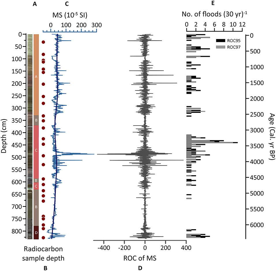
Figure 5. (A) Surface image of SA16/17 shown together with unit divisions (A–D). (B) Sampling depth for radiocarbon (¹⁴C) dates (red dots). (C) Magnetic susceptibility (MS, 10⁻⁵ SI) for the whole core plotted together with a superimposed trend line (quadratic Gaussian LOESS fit). (D) Rate of change (ROC) of MS (calculated on depth scale), which is presented in column C. (E) Flood reconstruction plotted against the age axis to the right. Each bar represents the number of floods per one 30 year period. The reconstruction of extreme floods is based on values crossing the 95th percentile of ROC based on the MS values (D; black bars). For comparison, the reconstruction was also made with values above the 97th percentile (gray bars).

Facies A (0–325 cm) was the most minerogenic facies of the core, with MS showing a flat trend around 40 * 10⁻⁵ SI with high variability (0–150 * 10⁻⁵ SI). The facies was laminated with alternating dark brown/black organic material with MS values close to the trend line (Figure 5C) and lighter colored silty layers with a peak MS (>100 * 10⁻⁵ SI). The thickest sand layer of facies A to C was in facies A at 90–95 cm and MS values were close to zero throughout the layer. The top 80 cm of the core was rather light beige/gray, changing to shades of brown and even black, with only one MS value peak above 100 * 10⁻⁵ SI. The ROC of MS naturally followed the variability of MS and had several peaks with ROC exceeding the 95th and 97th percentiles (Figures 5D,E).

In facies B, three core sections of different thicknesses at 325–368, 583–600, and 630–778 cm showed the same homogeneous organic matrix with no sedimentological structures. Radiocarbon samples from this facies contained plenty of macro-fossils, such as leaves, seeds, and twigs. MS had low variability throughout this facies (around 25 * 10⁻⁵ SI), following the MS trend line; the ROC was low. Only four peaks (between 580 and 697 cm depth in the core) had ROC values exceeding the 95th percentile. The thinnest B facies, at ~590 cm, had a bit more variability and higher MS values than the trend line (ca 25 * 10⁻⁵ SI) through all of facies B.

Facies C (368–583 and 600–630 cm) was similar to facies A, but the sediments were generally darker, reaching more toward black or reddish brown, in contrast to facies B, with its brown and beige sediments. Facies C exhibited higher variability in MS (0–285 * 10⁻⁵ SI) than observed in facies A, with increased MS in silt layers and values close to zero in the organics. This facies had the most ROC values exceeding the 95th and 97th percentiles, particularly the section between 478 and 550 cm depth in the core. The two thickest clay layers in the core (at ca. 577–584 and ca. 620–630 cm) were both in facies C, and the highest MS peak (284 * 10⁻⁵ SI) was in the uppermost of these facies, at 487 cm. One layer (at ~408 cm) only consisted of small wood pieces on top of a thin sand layer.

Facies D (778–830 cm) consisted of an organic matrix but maintained thick sand layers, including the two thickest sand layers of the whole composite core (at ca. 794–795 cm and 807–818 cm in depth). There was a 4 cm-thick organic layer with wet, non-moldered pieces, indicating high water content between the sandy layers. This yielded variability in MS (−24 to 100 * 10⁻⁵ SI) and consequently in ROC. High water content could explain the negative MS values in this facies.

The results from the grain size analysis show that the sand and clay layers have distinct grain size classes. The mean grainsize distribution of the sand layers are bimodal, with a coarse mode between 100 and 500 μm. The sand layers are interpreted to represent subaquatic slumping processes given the short proximity to the delta, and also because they only consisting of sand. In contrast, the clay layers have a clear unimodal distribution with a mode at about 10 μm that likely are glacigenic (cf. Røthe et al., 2019; Figure 6). This since the catchment is glaciated and glaciers are known for producing fine and bright clay particles such as found in the core. The grainsize of material with high MS plots between the glacial and slumping sediments indicating origin from another process. The relationship between χbulk_293K and median grain size showed no significant correlation, analyzing all samples as one group (Figure 7). Investigating the four sediment classes independently showed correlations in the background and slumping sediments but no correlation within the glacial (r² = 0.31, p = 0.68) or hypothesized flood sediments with high MS (r² = 0.11, p = 0.48).

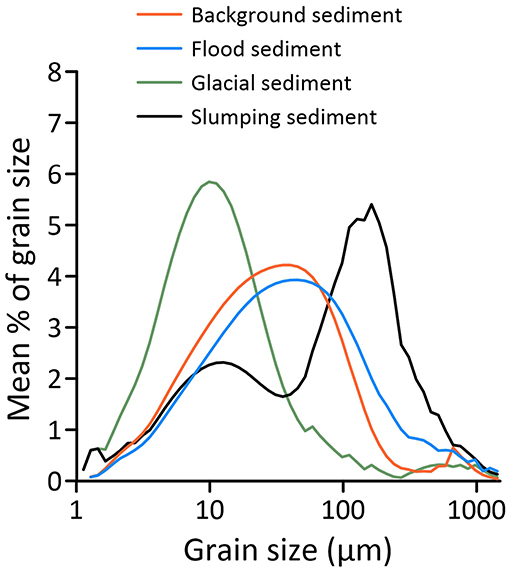
Figure 6. Mean grain size distributions for four sedimentary classes based on interpretation of the sedimentology and magnetic susceptibility (MS; sections Core SA16/17 and Sediment Sources): (i) background sediments, (ii) flood sediments (high MS), (iii) glacial sediments (clay, low MS), and (iv) sediments associated with slumping events (sand, low MS).

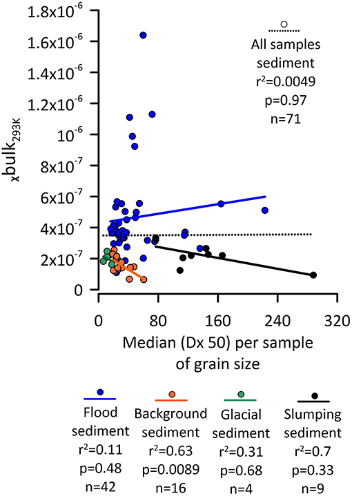
Figure 7. Correlation of the full grain size dataset vs. χbulk measurements at room temperature (293 K) indicates that magnetic susceptibility (MS) does not depend on grain size. Investigating the sedimentary classes independently, a correlation exists between the parameters for background and slumping sediments. Glacial and flood sediments do not show a significant relationship between median grain size and χbulk_293K/MS.

Core SAD616

The χbulk values from SAD616 followed the trend of the χbulk-values in SA16/17 (Figure 4) showing the similarities between the sediments in the cores. The χbulk values were below a ratio of two for all samples, indicating a dominance of ferromagnetic material in this core.

SAD616 (Figure 8) was 65 cm long and had gray-brown sediments with some red in the layers in the top 10 cm of the core. The matrix consisted of a mixture of clay, silt, and organic material. There was layering visible in the top 10 cm and between 15 and 20 cm of the core and at 56 cm and 63 cm. The MS trend line was relatively flat, around 42 * 10⁻⁵ SI the top 18 cm, but then increased to above 50 * 10⁻⁵ SI until 30 cm before decreasing. MS also showed variability as in SA16/17, fluctuating between 20 * 10⁻⁵ SI and 70 * 10⁻⁵ SI. The ROC was highest in the upper 30 cm of the core, with a maximum frequency of events exceeding the 95th percentile in the upper 15 cm.

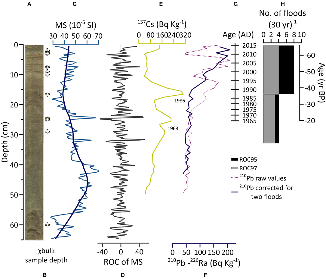
Figure 8. (A) Surface image of SAD616 core. (B) Pale yellow crosses show where samples that were measured for χbulk were taken. (C) Magnetic susceptibility (MS) of the core (10⁻⁵ SI) with its trend (quadratic Gaussian LOESS fit). (D) Rate of change (ROC) of MS. (E) Raw values of cesium (¹³⁷Cs) measurements used to date the upper part of the short core. The two peaks date to 1986 and 1962. One explanation for the double-1963 event is possibly the flood that occurred in 1962. The χbulk measurements at 24.5 cm are most likely ferromagnetic; all χbulk samples have a ratio below two (see Figure 4). (F) 210-Lead (²¹⁰Pb) measurements, same depth as ¹³⁷Cs; the dashed line shows raw values of the ²¹⁰Pb curve, while the solid line shows the corrected ²¹⁰Pb profile. It is corrected on the assumption of two floods (identified at ca. 4 and 8 cm) bringing in old ²¹⁰Pb to the core location from land, which would explain why ²¹⁰Pb dips toward zero. (G) Extrapolation of AD ages between the two peaks in ¹³⁷Cs and 2016 when the core was retrieved. Note that these leave two different sedimentation rates for the two periods in question, namely 0.55 cm yr⁻¹ between 1986 and 2016 and 0.40 cm yr⁻¹ between 1963 and 1986. (H) Flood frequency based on the ROC of MS (D) above the 95th (black) and 97th (gray) percentiles, plotted against the age axis to the right (yr BP). Note that we only have dated ROC-floods from 1963 so the number of floods in the 30 year period between 1956 and 1986 actually occur between 1963 and 1986.

Chronology

The age–depth model for SA16/17 showed continuous sedimentation back to ~6,500 cal. yr BP (Figure 9). The 26 analyzed radiocarbon dates (Table 1) were distributed over the full 830 cm-long core (SA16/17), and the age-depth model showed a good fit for most of the radiocarbon samples. The individual calibrated ages had an uncertainty between ±12 and ±45 years. The age model had an uncertainty range between 84 and 582 years. Most of the largest uncertainties were close to the bottom of the age-model curve (Figure 9).

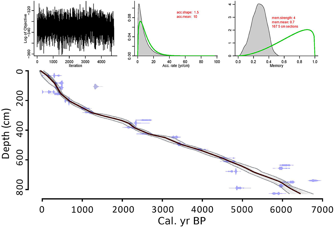
Figure 9. Age–depth model output from the software Bacon (Blaauw and Christen, 2011). The model is based on 26 radiocarbon dates (blue marks), and the associated age probabilities for each individual sample are shown. Some radiocarbon dates were rejected as they deviated notably from the overall best fit (see section Chronology).

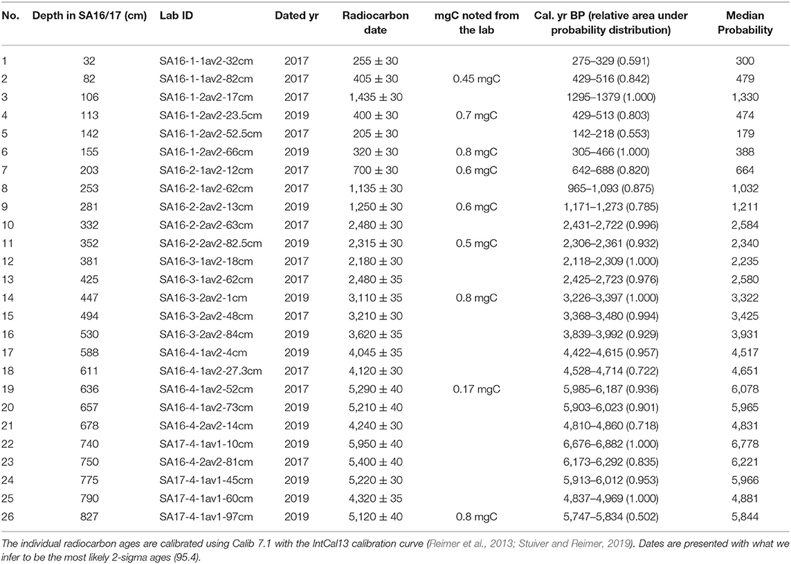
Table 1. Summary of the 26 radiocarbon samples (terrestrial plant remains) analyzed at the Poznan Radiocarbon Laboratory.

We chose to use only ¹³⁷Cs to construct an age model of the core SAD616. This was done because the ²¹⁰Pb-profile (Figure 8F) seemed to have been disturbed by flooding events. ²¹⁰Pb drops to zero when old lead was washed from the catchment to the lake during floods. As a test one ²¹⁰Pb profile in Figure 8F was corrected for two assumed floods based on the ²¹⁰Pb value being close to zero. However, we did not use it further. ¹³⁷Cs had two marked peaks; one was interpreted to be the ¹³⁷Cs event in 1986 AD (Chernobyl nuclear power plant accident) and the other in AD 1963 (nuclear bomb test). The second peak was disturbed (divided into two peaks), likely by one or more floods. There was one large historical flood documented in AD 1962, supporting this argument. Hence, we used the largest of the two local peaks at about 25 cm as AD 1963 (Figure 8E). Thus, the age model for SAD616 was based on two clear peaks in ¹³⁷Cs, observed in AD 1963 and AD 1986 (Figure 8E), and AD 2016 represented the top of the core (the year it was retrieved). The ages were linearly extrapolated between these dates (Table 2 and Figure 8) to produce an age-depth model. The sedimentation rate was different between the sections, 0.4 cm yr⁻¹ between AD 1963 and AD 1986 and 0.55 cm yr⁻¹ between AD 1986 and AD 2016.

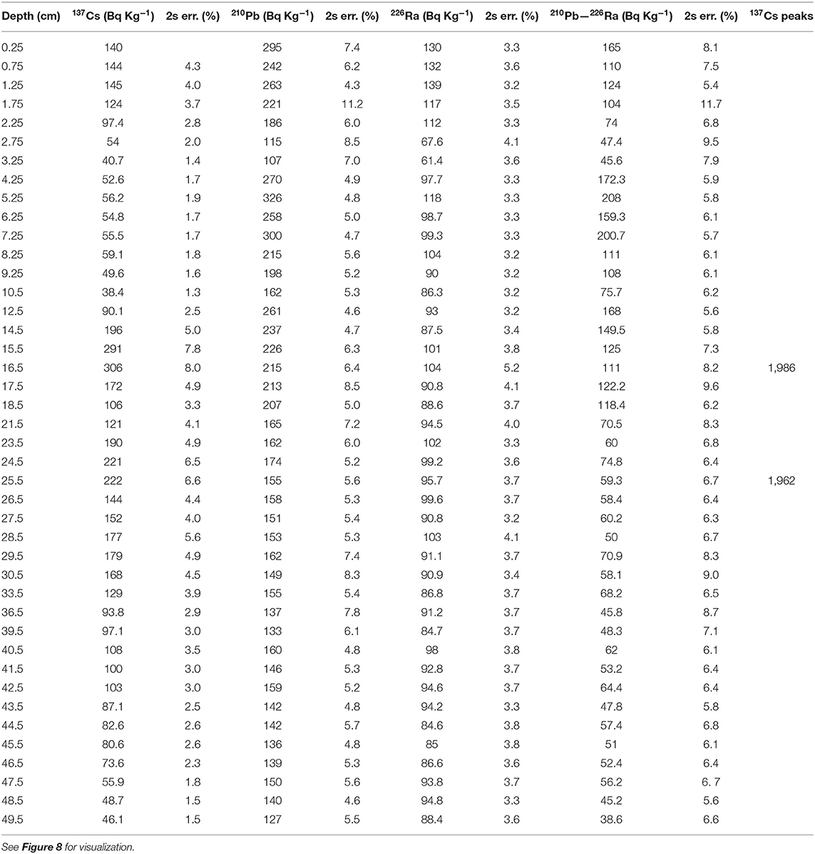
Table 2. ²¹⁰Pb, ²²⁶Ra, and ¹³⁷Cs measurements of SAD616.

SA16/17s ended in AD 1984 (−34 cal. yr BP) and was correlated with SAD616 using its age model starting in AD 1963. The record ended in AD 2016, when the cores were retrieved. Figure 10 shows a schematic illustration of how the cores were merged, with SA16/17 as a composite core based on visual logging, MS, and age and SAD616 on top based only on the age correlation.

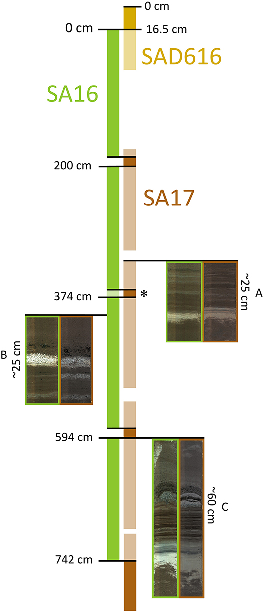
Figure 10. Image showing how the three cores from Lake Sandvinvatnet are stacked: SAD616 (yellow) at the top; the main piston core, SA16 (green), to the left; and the piston recovery core, SA17 (brown), to the right. The shaded parts of the cores are not included in this study. The composite core is correlated mostly with visual layers, as exemplified by sections (A–C). At the top and bottom of SA17, age and magnetic susceptibility (MS) are employed to guide the inter-core correlation. SAD616 is correlated only by age. *At this depth, the two cores have different compaction rates; hence, there is no space between SA16 at this depth when compared with SA17.

Discussion

Sediment Sources

Lake Sandvinvatnet is a sink for sediments both produced in the catchment (autochthone) and in the lake (allochthon). Based on laboratory analyses, we have unraveled the different sediment sources and conducted a fingerprinting of the sediments related to flood events. The χbulk analysis of the sediment cores SA16/17 and SAD616 suggest that there is predominantly one source area for the ferromagnetic material found in the lake sediments (Figure 11, section Core SA16/17). We suggest that the point source for the sediments comes via the delta at the mouth of Buerdalen (Figure 1A). The orientation of Jordalselvi entering the lake (Figure 1A) appears to have been stable over the last decades (Statens kartverk, 2020), and there is no evidence from the field survey suggesting that this changed during the time span covered by the sediment core. Buerdalen is the only sub-catchment of Sandvinvatnet with a glacier, and the presence of glacial flour (silt and clay) in the core supports Buerdalen as a sediment source (Karlén, 1976; Bakke et al., 2005a). Moreover, the coring site is close to the inlet of Jordalselvi, and the sediments contain relatively coarse sandy layers that are suggested to stem from the delta. Therefore, it is reasonable to assume that the Buerdalen valley is the main source area for the material arriving at the core site (Figures 1A, 3). These observations do not rule out that, at times, sediments may also have been delivered from the eastern slopes and southern inlet. However, there are only small water pathways at the east side of the lake. The depth of the lake and the considerable distance that the sediments would have to travel from the southern inlet all the way to the coring site suggest that the potential contribution from the eastern and southern sides of the lake is negligible compared with the influx from Buerdalen.

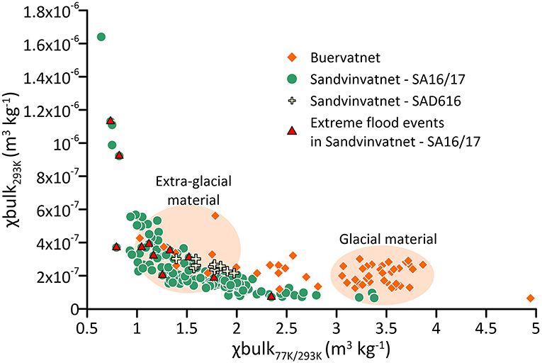
Figure 11. χbulk_293K and χbulk_77K/293K values from samples measured both on sediments from Lake Sandvinvatnet and Lake Buervatnet (Figure 1). The shaded orange areas highlight the two main sedimentary classes in Buervatnet (Røthe et al., 2019). These are organic material with ferromagnetic carriers (χbulk_77K/293K from roughly 1–2.5), and glacial outburst floods (GLOFs) plus glacial material returning high χbulk_77K/293K values indicative of paramagnetic dominance. The χbulk dataset from Sandvinvatnet (green dots/pale yellow crosses) and Buervatnet (orange squares) summarize a more complete view of sediment sources and magnetic properties of the Buerdalen valley.

Since floods and hazardous events heavily influence the catchment, the radiocarbon dated outliers (nine) were most likely re-worked organic material from the catchment. From the radiocarbon laboratory, it was noted that eight of the radiocarbon samples had low pure carbon concentrations, and therefore, the results need to be handled with care (Table 1). However, except for two samples at the bottom of the core, these followed the modeled age–depth relationship closely (Figure 9).

Magnetic Signature and Geomorphic Processes in the Valley Buerdalen

Magnetic properties of sediments and soils in a catchment may undergo chemical and physical alterations. This typically occurs when sediments are exposed to erosion, weathering, and/or soil production (Thompson and Oldfield, 1986). The sediments evacuated from Buerdalen consist of different magnetic components, suggesting that there was more than one source area, as well as possible secondary processes, although the latter question has not been examined in detail. Røthe et al. (2019) showed, for instance, that in Buervatnet, the small lake in the upper part of the Buerdalen catchment (Figure 1A), paramagnetic carriers dominate the sedimentation into the lake during GLOF events and general glacial erosion (Figure 11). This is in accordance with the local granitic bedrock, and therefore, is most likely the primary magnetic carrier from Buerdalen to reach Sandvinvatnet. From this, it can be inferred that the ferro/ferrimagnetic carriers must come from elsewhere and/or also be the result of secondary processes. It should be noted that, whenever there is a GLOF, sediments freighted with it will be depleted upon entering Buervatnet—the first basin—and hence, the subsequent delivery further downstream will be filtered and reduced. Consequently, the runoff associated with GLOFs are not necessarily as large as one might expect. A local farmer noted that discharge in Jordalselvi during the GLOF in 2002 was considerable (Røthe et al., 2019) but not hazardously increased. Apart from GLOFs, normal glacier activity will mostly modulate the signal in Sandvinvatnet though the magnitude and timing of the meltwater added to the overall runoff budget.

Following the argumentation given above, material with high MS is correlated with a low MS ratio, indicating an extra-glacial source in Buerdalen. Thus, distinct layers with a rapid increase in MS (marked by ROC exceeding the 95th and 97th percentiles) are likely to represent flood deposits containing re-deposited ferromagnetic material transported to Sandvinvatnet by Jordalselvi.

Grain size analysis supports this hypothesis, as the ferromagnetic flood deposits are clearly different from both the fine-grained glacial-derived sediments and coarse-grained slumping sediment, which are paramagnetic. The slumping events could indirectly be triggered by a flood. Grain sizes in sediments following the intermediate (Gaussian loess fit) MS values have a similar distribution to the flood material. This indicates that the source of the flood material is the same during “normal” runoff conditions, and the transport of material only increases during a flood event rather than originating from a different source area. The wood pieces resting on top of a sand layer (facies C, 412 cm depth in SA16/17, Figure 5) may have been transported into the lake by a snowslide/slushflow originating from the eastern shore of the lake, or we may simply have hit a tree trunk on the lakebed while coring. The absence of disturbances to this layer favors the latter interpretation. The layer does not have the same magnetic signature as a flood event, which is why we do not interpret it to be deposited by a flood. Although we cannot exclude the possibility, that some sediments originated from the eastern slopes, the bedrock in that part would probably yield diamagnetic or paramagnetic rather than ferromagnetic sediments. This is because the bedrock on top of the eastern plateau is quartz rich, and the slopes are steep, not allowing material to stay long enough to produce the same amount of ferromagnetic sediments as in Buerdalen. The very low and even negative MS values in facies D of the composite core could indicate diamagnetic material potentially related to landslide and/or avalanche processes in this area, if not subglacial processes retaining organic material. The sediments in facies D also have high water content compared with the rest of the core, and since water is diamagnetic, it can partially explain the low MS values, and hence, the large ROC values in this facies. The thick macrofossil layer in this facies could also be from penetrating an old tree trunk or vegetation hub.

We have argued that the ferromagnetic carriers are produced and originating from the catchment through weathering of landslide, avalanche, and rock fall deposits along the steep valley slopes in Buerdalen (Figure 1A; cf. Thompson and Oldfield, 1986). These sediments are likely channeled to the stream at the valley floor by snowmelt (spring) and rain (fall), especially during intense rain events and storms when the soils are already saturated. The river carries these sediments to Sandvinvatnet, where they are deposited. This interpretation tends to suggest that the size of the floods should be proportional to the strength of the MS signal, which is not what we observe, nor is it the case when compared with historical data (5.2). One possible explanation for that is that, if several floods occur within a short timespan, the material on the slopes in Buerdalen available for remobilization would already be somewhat depleted and vice versa. Moreover, the discharge and amount of material transported will also depend on how saturated the catchment is prior to the flood commences. This balancing act between climate trends and catchment characteristics hinders us from making any inferences about flood size. Importantly, it means that the floods recorded in Sandvinvatnet are relatively large, and this condition prevails throughout the record.

Paleo Proxy Data vs. Historical Floods

By comparing the two datasets of χbulk-analysis of Buervatnet and Sandvinvatnet, it appears that the flood sediments have a relatively increased ferromagnetic component compared with sediments derived from direct glacial erosion and GLOFs, which are more paramagnetic. Given that the sediments in the Buerdalen catchment tend to be influenced by ferromagnetic carriers originating from the valley slopes, the “normal” or mean magnetic signal borders between the para- and ferromagnetic response having a ratio around two (Figure 11).

We record the frequency of the most extreme flood events by quantifying the number of events exceeding the 95th and 97th percentiles of ROC of MS. The recorded historical floods in the area (Roald, 2013; Kraftmuseet, 2019) overlap with the reconstructed flood variability based on the sediment cores (Figure 12) and indicate that MS variability (ROC of MS) is indeed related to flood events and that rapid changes in MS are a reliable diagnostic tool to identify flood deposits. Not all these events reach the 95th percentile, indicating that this threshold is somewhat conservative and may not catch all extreme floods in this catchment; it also suggests that the signal-to-noise ratio is high. The uncertainties in the age model beyond the ¹³⁷Cs peak may be what causes the extremely small offsets for the twentieth century floods. The uncertainty range for the ages in the composite core based on SA16/17 in the top 280 years is between 107 and 220 years. SAD616 is correlated to the cores SA16/17 based on the rough radiocarbon age estimate and is plotted from AD 1963 in Figure 12.

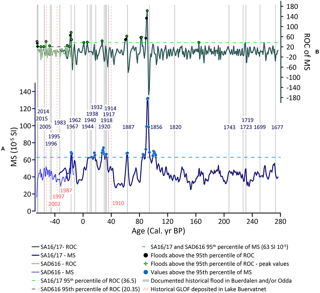
Figure 12. (A) Magnetic susceptibilities (MSs) of both SA16/17 (dark blue line) and SAD616 (bright blue dotted line) correlated using their age from 1963 AD (−13 yr BP). (B) Rate of change (ROC) of both SA16/17 (dark green line) and SAD616 (bright green dotted line) correlated using their age from 1963 AD (−13 yr BP). Historical documented floods (gray bars) are compared with glacial outburst floods (GLOFs) from Buervatnet (orange striped bars) and MS (blue dots) and ROC (black dots) values above the 95th percentile. The ROC values above the percentile are data points included in the two flood reconstructions with, all (black dots) and peak values only (green crosses; Figure 13). The documented floods and GLOFs are presented with the year (AD) that they occurred (Roald, 2013; Kraftmuseet, 2019). The maximum uncertainty range of the ages for the SA16/17 is 107–220 years in the top 280 years.

Climate and Flood Variability During the Past 6,500 Years

The Holocene climate in Northern Europe has shifted between warm and cold periods, with some more pronounced than others (Ljungqvist, 2011; Wanner et al., 2015). The Holocene thermal maximum (HTM) 8,300 to 4,000 cal. yr BP (Ljungqvist, 2011) was warmer and less humid than at present. The record from Sandvinvatnet covers the end of HTM (5,000–4,000 cal. yr BP), through the neoglacial (onset around 4,000 cal. yr BP), until the present day. Two additional warmer periods occurred 2,000–1,000 cal. yr BP, and the past 150 years, but they did not reach equally warm temperatures as during the HTM (Seppä et al., 2009). The warm periods have been coupled to the historical periods, the Roman Warm Period (RWP) around 2000 cal. yr BP and the Medieval Warm Period (MWP) around 1,000 cal. yr BP (Mann, 2007). Two cold periods occurred between cal. 3,800 cal. yr BP and 3,000 cal. yr BP as well as between 500 and 100 cal. yr BP, the last period known as the LIA (Seppä et al., 2009). During both periods, the July temperature was lower than the present in Northern Europe and at our study site. In western Norway, the LIA is correlated to lower summer temperatures and an increase in winter precipitation (e.g., Bjune et al., 2005).

Comparing the flood frequency diagram using all ROC values above the percentiles and only using the highest peak values for the floods show the same trend. Overall the periods with more or less floods also concur. The number of floods are lower using only the peak values which we expect using less ROC values. One ROC peak with several values could belong to the same flood, especially if the peak is sharp (e.g., Figure 12, the flood year AD 1856). However, sediment layers can be very thin and the limited resolution of the datasets could merge several events together as one peak, especially where the peak is vague. This is very clear in MS (Figure 12; e.g., floods AD 1914–1920) even though not all of the values reach the 95th percentile in ROC. Since we discuss trends in flood frequency rather than the exact number of floods, we continue discussing all ROC values above the 95th and 97th percentiles, and not peak ROC values marking the onset of individual flood events. This is done to avoid subjective interpretation of when a flood deposit ends, and another begins. Both flood frequency diagrams are presented in Figure 13.

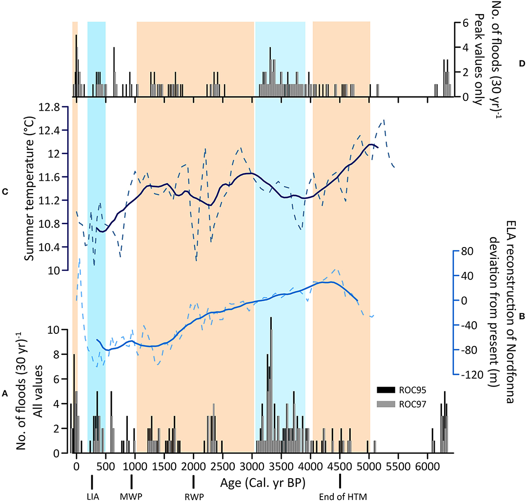
Figure 13. (A) Flood frequency diagram based on the rate of change (ROC) of magnetic susceptibility (MS) for both the SA16/17 and SAD616 cores using all values above the 95th (black) and 97th (gray) percentiles. (B) Glacier reconstruction of Nordfonna—located <17 km north of Buerdalen valley—as evident from altitudinal shifts in the local equilibrium line altitudes (ELAs) compared with present day (Bakke et al., 2005b). (C) Local summer temperature reconstruction from Vestre Øykjamyrtjørn <40 km southwest of Sandvinvatnet (Bjune et al., 2005). (D) Flood frequency diagram based on ROC of MS for both the SA16/17 and SAD616 cores using only the peak values above the 95th (black) and 97th (gray) percentiles. The orange and blue markings represent warm and cold periods delineated by Seppä et al. (2009).

The flood reconstruction from Sandvinvatnet shows a flood frequency in 30 year periods for the last 6,500 cal. yr BP, up to AD 2016 (Figures 13A,D). The number of floods varies significantly through time, especially one time interval (4,100–3,140 cal. yr BP) with an abundance of 30 year periods of extreme floods. Between 3,140 cal. yr BP and AD 2016 (−66 cal. yr BP) there are five clusters of four or more 30 year periods succeeding each other (around 4,300, 1,700, 1,400, 400 cal. yr BP and the last 150 cal. yr) interrupted by periods of no floods at all. The longest time interval with no extreme floods is 960 years long (6,140–5,180 cal. yr BP). Between 6,290 and 4,100 cal. yr BP the frequency of floods is comparably low, having three or fewer succeeding 30 year periods disrupted by intervals with no floods. The earliest 200 years in the record are marked by succeeding flood 30 year periods. The number of floods in each 30 year period varies between one and twelve (one and six for the flood frequency based on peak values only). The highest number of extreme floods occurred between 3,400 and 3,100 cal. yr BP and during the past 600 years (Figure 13A). Compared with the floods above the 97th percentile of ROC, the 95th percentile generally shows higher flood counts.

Driver of the Flood Variability Recorded in Lake Sandvinvatnet

Our flood reconstruction differs somewhat from previous flood reconstructions from eastern Norway. Studies from other locations in southern Norway, on the eastern side of the water divide, show almost the opposite trend in flood frequency during the last 6,500 years (Støren et al., 2010, 2012). The difference can be explained in that these sites are located on each side of the mountain chain and do not share the main flood origin and patterns. In the present climate, rainfall-induced floods in western Norway are mainly caused by changes in the westerlies and transport of humid air toward the coast, whereas precipitation in eastern Norway is mainly caused by air flows from the south and southeast (e.g., Lawrence, 2020). Further, floods in eastern Norway are strongly influenced by snowmelt, and the climatic driver of these floods is linked to winter precipitation, atmospheric patterns, and feedback mechanisms from the catchments (Støren et al., 2010, 2012; Støren and Paasche, 2014).

Extreme floods in western Norway are driven by extreme rain to a larger extent than in eastern Norway (Roald, 2013). Figure 2 shows the seasonality of independent floods above 25 m³s⁻¹, representing the 98% quantile of the daily flows since 1958 and contribution from rain vs. snow. All values are based on gridded SeNorge models for precipitation, temperature, snowmelt, and runoff (NVE et al., 2020) extracted for the Buerdalen catchment. It shows a flood season with a clear bimodal separation of the rain and melt floods in the Buerdalen. The floods in June through August are clearly influenced by snow- and glacial melt (red dots in Figure 2), but the fall floods are mostly caused by rain. The rain floods more often have higher discharge than the floods dominated by melt. We know from historical data that the largest floods are often caused by intense rain but sometimes increased by snow and/or glacial melt (Roald, 2008, 2013). The historical record agrees with present-day observations. Therefore, we argue that rain-induced floods were the most common floods at Sandvinvatnet throughout the Holocene, although we note that reconstructions point to cooler summer temperatures and high winter precipitation; on average, these findings would mean that more snow would be available to flooding and that the timing of the flooding could be shifted towards summer. This would suggest that atmospheric events causing intense rain (low-pressure systems and atmospheric rivers) have been the main drivers of floods backward in time. Variability of these events would be a large part of the flood frequency variation in Sandvinvatnet.

To support our assumption, we compared flood reconstructions to other archives. However, we could not find an obvious correlation of the flood frequency in Sandvinvatnet with, for example, reconstructions of sea surface temperatures based on various proxies (Thornalley et al., 2009; Orme et al., 2018), the North Atlantic Oscillation (NAO; Olsen et al., 2012), and storm track variability (Bakke et al., 2008; Orme et al., 2017). The glacial retreat and advance pattern for Folgefonna do not correlate with the flood-reconstructed variability in Sandvinvatnet (Figure 13B). Previous studies have shown that winter precipitation and glacial growth in southwest Norway are strongly linked to the NAO trending toward a positive state (Nesje et al., 2008). Consequently, this excludes glacial retreat/advance, winter precipitation, and the NAO as the main climatic driver of extreme floods in our study area.

For summer temperatures in Northern Europe (Seppä et al., 2009), local summer temperatures (Bjune et al., 2005) and the flood reconstruction still do not show a strong correlation (Figure 13). Keeping in mind that many of the climate reconstructions only concern summer temperatures, a complete match is not to be expected, since most floods occur during fall in our study area. The extreme flood interval during 4,100–3,140 cal. yr BP falls under one of the cold intervals from Seppä et al. (2009). There is also an increase in extreme floods during the LIA. A colder and more humid climate would increase snow in the mountains and contribute to glacial growth. More snow and ice would increase the number of melt-induced floods and provide more melt in the catchment overall. More melting during storms would cause even more extreme flood situations.

Two warmer intervals (Seppä et al., 2009) are evident during periods with no floods or small clusters of floods in Sandvinvatnet. A warmer and drier climate would have less precipitation and less precipitation falling as snow, possibly decreasing the number of floods. However, higher temperatures would increase the melting of the snow and glaciers. This may not be enough to cause an extreme flood by itself, but together with rain and less frozen ground during the winter, floods could be extreme nonetheless.

Future Flood Variability

For southwest Norway, the climate models suggest 1.5–2°C warming in the coming four decades together with a 23–46% increase in precipitation, depending on what climate scenario is used (Lundstad et al., 2018). Therefore, floods caused by heavy precipitation are predicted to increase both in magnitude and in frequency (Norwegian Climate Service Center, 2017; Lawrence, 2020). Until the end of this century, days with extreme precipitation are expected to increase threefold (Lundstad et al., 2018), which could cause increased vulnerability for the city of Odda and surrounding infrastructure as the most severe floods are caused by intense rain events at present. In areas with steep terrain, where the discharge response is fast, an increase in precipitation can become a serious challenge. Future climate scenarios suggest less snow, which will have an effect on the flood type in mountainous areas; snowmelt will decrease as a component in extreme floods in western Norway even more. For the valley of Buerdalen, which has a 50% glacier cover, the increased temperature may lead to increased melt water runoff, contributing to floods in the Buerdalen catchment. Since the climate projections indicate a warmer and wetter climate, the situation in the future may be different from any other time interval seen during the late Holocene.

The most recent 30 year period has nine floods, representing the highest flood frequency in the entire reconstruction (at the 95th percentile). The preceding period also showed a substantial number of floods, five. However, these two climatic periods are too short to draw any firm conclusions about present-day trends. Having said that, two large historical floods in the last six years and the abundance of floods in the last two climatic (30 year) periods in the flood reconstruction could be interpreted as a forewarning of what to expect of the near future.

The reconstructed floods above the 95th percentile show the largest and most extreme floods, and the method does not record smaller floods. As seen in the comparison with historical floods, some of these have caused local damage although they have not reached the 95th percentile.

Conclusion

This study used MS and χbulk measurements of an 830 cm-long sediment core from Sandvinvatnet to reconstruct extreme flood frequency in southwest Norway during the past 6,500 years, documenting variability in frequency over time. We observe intervals with more extreme floods than on average. Intervals include the period from 4,100 to 3,140 cal. yr BP and also several shorter intervals such as 6,500–6,050 cal. yr BP, during LIA as well as the last 150 years. Conversely, we observe no extreme floods for prolonged periods of time including 6,050–5,420, 3,140–2,570, and 2,210–1,850 cal. yr BP. The number of floods per 30 year period varied between one and nine.

The extreme flood record presented in this study is the first of its kind from the western part of Norway. Flood reconstructions from eastern Norway show a different extreme flood history. The contrast between east and west is possibly explained by rain-induced vs. snowmelt-induced floods and different weather patterns causing high precipitation in these two regions. Floods in western Norway are highly dependent on intense rain, caused by the strength of the westerly wind belt and its transport of humid air toward the coast; floods in eastern Norway are more often caused by snowmelt, sometimes combined with rain connected to easterly and southerly wind flow regimes. The fall storms occurring at Sandvinvatnet are caused by low-pressure systems arriving from the Atlantic, sometimes acting as atmospheric rivers transporting humid air from lower latitudes. Climate analogs to the past indicate more floods during relatively wet and cold intervals with access to snow- and ice melt and fewer floods in relatively warm and dry periods. Since the climate projections indicate a warmer and wetter climate, there is no past climate analog, and the future may be different from any other time interval seen during the late Holocene.

Data Availability Statement

The raw data supporting the conclusions of this article will be made available by the authors, without undue reservation.

Author Contributions

The study was designed and planned by JB and FE. FE structured the work, planned the laboratory work, wrote the main part of the manuscript, and also conducted most of the laboratory work. JB, ES, FE, and FA carried out the lake coring and fieldwork. ØP, JB, and ES contributed to the analysis of the datasets in this study and supported the writing of the manuscript. KE contributed Figure 2 and the knowledge about the modern age flood situation in the study area, as well as editing the manuscript. All authors contributed to the article and approved the submitted version.

Funding

HORDAFLOM (269682) financed this study with additional input from TRANSENERGY.

Conflict of Interest

The authors declare that the research was conducted in the absence of any commercial or financial relationships that could be construed as a potential conflict of interest.

Acknowledgments

The Bjerknes Centre for Climate Research (HORDAFLOM and CHEX) supported this study with a network for scientific discussions and collaboration with municipalities that will benefit from this study. Thank you to Jordan Donn Holl and Lubna Al-Saadi for good and efficient lab work, which was highly valued. All analyses were done at the National Infrastructure EARTHLAB (NRC 226171) at the University of Bergen. Fieldwork support was provided by students in the GEOV226 course (2016) and Emmauel Malet.

Supplementary Material

The Supplementary Material for this article can be found online at: https://www.frontiersin.org/articles/10.3389/feart.2020.00239/full#supplementary-material

References

Alnes, K., Berg, A. O., Clapp, C., Lannoo, E., and Pillay, K. (2018). Flomrisiko i Norge: Hvem Betaler for Framtidens Våtere Klima? Oslo. Available online at: https://cicero.oslo.no/no/publications/internal/2872 (accessed July 23, 2020).
Azad, R., and Sorteberg, A. (2017). Extreme daily precipitation in coastal western Norway and the link to atmospheric rivers. J Geophys Res Atmos. 122, 2080–2095. doi: 10.1002/2016JD025615
Bakke, J., Dahl, S. O., and Diesen, M. (2000). Folgefonna Nasjonalpark. Bergen: University of Bergen.
Bakke, J., Dahl, S. O., and Nesje, A. (2005a). Late glacial and early holocene palaeoclimatic reconstruction based on glacier fluctuations and equilibrium-line altitudes at northern Folgefonna, Hardanger, western Norway. J. Quat. Sci. 20, 179–198. doi: 10.1002/jqs.893
Bakke, J., Lie, Ø., Dahl, S. O., Nesje, A., and Bjune, A. E. (2008). Strength and spatial patterns of the Holocene wintertime westerlies in the NE Atlantic region. Glob. Planet. Change 60, 28–41. doi: 10.1016/j.gloplacha.2006.07.030
Bakke, J., Lie, Ø., Nesje, A., Dahl, S. O., and Paasche, Ø. (2005b). Utilizing physical sediment variability in glacier-fed lakes for continuous glacier reconstructions during the holocene, northern Folgefonna, western Norway. Holocene 15, 161–176. doi: 10.1191/0959683605hl797rp
Bjune, A. E., Bakke, J., Nesje, A., and Birks, H. J. B. (2005). Holocene mean July temperature and winter precipitation in western Norway inferred from palynological and glaciological lake-sediment proxies. Holocene 15, 177–189. doi: 10.1191/0959683605hl798rp
Blaauw, M., and Christen, J. A. (2011). Flexible paleoclimate age-depth models using an autoregressive gamma process. Bayesian Anal. 6, 457–474. doi: 10.1214/ba/1339616472
Blöschl, G., Hall, J., Parajka, J., Perdigao, R. A. P., Merz, B., Arheimer, B., et al. (2017). Changing climate shifts timing of European floods. Science 357, 588–590. doi: 10.1126/science.aan2506
Bøe, A.-G., Dahl, S. O., Lie, Ø., and Nesje, A. (2006). Holocene river floods in the upper glomma catchment, southern Norway: a high-resolution multiproxy record from lacustrine sediments. Holocene 16, 445–455. doi: 10.1191/0959683606hl940rp
Climate-data.org (2020). Klimat Odda. Available online at: https://sv.climate-data.org/europa/norge/hordaland/odda-9915/ (accessed May 17, 2020).
Dannevig, H., Groven, K., and Aall, C. (2016). Naturfareprosjektet - Oktoberflaumen på Vestlandet i 2014 (Oslo). Available online at: https://www.vestforsk.no/nn/publication/oktoberflaumen-pa-vestlandet-2014. Report 2016-3 (accessed March 20, 2019).
Davies, R. (2014). 100s Evacuated After Major Flooding in Western Norway. Available online at: http://floodlist.com/europe/major-flooding-west-norway (accessed February 18, 2019).
Engeland, K., Holmqvist, E., and Orvedal, K. (2018a). Beregning av dimensjonerende flom i Mandalsvassdraget ved Kjølemo – hvor avgjørende er datagrunnlaget? Vann 3, 283–296.
Engeland, K., Wilson, D., Borsányi, P., and Roald, L. (2018b). Use of historical data in flood frequency analysis: a case study for four catchments in Norway. Hydrol. Res. 49, 466–486. doi: 10.2166/nh.2017.069
Geological Survey of Norway (NGU) (2016). Earth Deposits Map of Norway. Available online at: http://geo.ngu.no/kart/losmasse_mobil/ (accessed July, 2, 2019).
Geological Survey of Norway (NGU) (2020). Bedrock Map of Norway. Available online at: http://geo.ngu.no/kart/berggrunn/ (accessed July 2, 2019).
Gunn, D. E., and Best, A. I. (1998). A new automated nondestructive system for high resolution multi-sensor core logging of open sediment cores. Geo Mar. Lett. 18, 70–77. doi: 10.1007/s003670050054
Hanssen-Bauer, I., Førland, E. J., Haddeland, I., Hisdal, D., Lawrence, S., Mayer, A., et al. (2015). Klima i Norge 2100. The Norwegian Centre for Climate Services Report M-406. Available online at: https://www.miljodirektoratet.no/publikasjoner/2015/september-2015/klima-i-norge-2100/ (accessed April 17, 2020).
Jackson, M., and Ragulina, G. (2014). Report No. 83 – 2014 Inventory of Glacier-Related Hazardous Events in Norway. Majorstua: Norwegian Water Resources and Energy Directorate (NVE).
Karlén, W. (1976). Lacustrine sediments and tree-limit variations as indicators of holocene climatic fluctuations in Lappland, Northern Sweden. Geogr. Ann. A 58, 1–34. doi: 10.1080/04353676.1976.11879921
Kartverket/norgeskart.no (2020). Høydedata. Available online at: https://hoydedata.no/LaserInnsyn/ (accessed March 17, 2020).
Kjøllmoen, B. (2004). Jøkulhlaup Sør for Svartenut. Reiserapport 23/04, Seksjon HBM. Oslo: Norwegian Water Resources and Energy Directorate (NVE).
Kobierska, F., Engeland, K., and Thorarinsdottir, T. (2018). Evaluation of design flood estimates—a case study for Norway. Hydrol. Res. 49, 450–465. doi: 10.2166/nh.2017.068
Kraftmuseet (2019). Flaum og Ekstremver i Sørfjorden. Available online at: http://www.nvim.no/flaum/flaum-og-ekstremver-i-sorfjorden-article475-1055.html (accessed January 24, 2019).
Kvisvik, B. C., Paasche, Ø., and Dahl, S. O. (2015). Holocene cirque glacier activity in Rondane, southern Norway. Geomorphology 246, 433–444. doi: 10.1016/j.geomorph.2015.06.046
Lawrence, D. (2016). Klimaendring og Framtidige Flommer i Norge. Oslo. Available online at: http://publikasjoner.nve.no/rapport/2016/rapport2016_81.pdf (accessed March 6, 2020).
Lawrence, D. (2020). Uncertainty introduced by flood frequency analysis in projections for changes in flood magnitudes under a future climate in Norway. J. Hydrol. Reg. Stud. 28:100675. doi: 10.1016/j.ejrh.2020.100675
Lawrence, D., and Hisdal, H. (2011). Hydrological Projections for Floods in Norway Under a Future Climate. NVE Report. Oslo. Available online at: https://www.nve.no/om-nve/publikasjoner-og-bibliotek/publikasjoner (accessed July 23, 2020).
Ljungqvist, F. C. (2011). The Spatio-Temporal Pattern of the Mid-Holocene Thermal Maximum. Geografie-Sbornik CGS 116.2: 91-110. Available online at: http://urn.kb.se/resolve?urn=urn:nbn:se:su:diva-59030 (accessed July 23, 2020).
Lundstad, E., Håvelsrud Andersen, A. S., and Förland, E. J. (2018). Klimarapport for Odda, Ullensvang og Jondal Temperatur og nedbør i Dagens og Framtidens Klima. Odda. Available online at: https://cms.met.no/site/2/klimaservicesenteret/rapporter-og-publikasjoner/_attachment/13607?_ts=1641d2576b5 (accessed March 10, 2020).
Mann, M. E. (2007). Climate over the past two millennia. Annu. Rev. Earth Planet. Sci. 35, 111–136. doi: 10.1146/annurev.earth.35.031306.140042
Møller, J., and Holmeslet, B. (2012). Havets Historie i Fennoskandia og NV Russland. Program ver. Jan 2012. Available online at: http://geo.phys.uit.no/sealev/index.html (accessed May 19, 2020).
Nesje, A., Bakke, J., Dahl, S. O., Lie, Ø., and Matthews, J. A. (2008). Norwegian mountain glaciers in the past, present and future. Glob. Planet. Change 60, 10–27. doi: 10.1016/j.gloplacha.2006.08.004
Nesje, A., Dahl, S. O., Matthews, J. A., and Berrisford, M. S. (2001). A ~ 4500-yr record of river floods obtained from a sediment core in Lake Atnsjøen, eastern Norway. J. Paleolimnol. 25, 329–342. doi: 10.1023/A.1011197507174
Norwegian Climate Service Center (2017). Klimaprofil Hordaland. Available online at: https://cms.met.no/site/2/klimaservicesenteret/klimaprofiler/klimaprofil-hordaland/_attachment/13183?_ts=16243d9ca17 (accessed March 10, 2017).
Norwegian Climate Service Center (2020). Gjor deg Klar for Fremtidens Vaer. Available online at: https://klimaservicesenter.no/ (accessed April 17, 2020).
NVE Met.no, Kartverket. (2020). SeNorge. Available online at: http://www.senorge.no/aboutXgeo.html (accessed April 6, 2020).
Olsen, J., Anderson, N. J., and Knudsen, M. F. (2012). Variability of the North Atlantic oscillation over the past 5,200 years. Nat. Geosci. 5, 808–812. doi: 10.1038/ngeo1589
Orme, L. C., Charman, D. J., Reinhardt, L., Jones, R., Mitchell, F., Stefanini, B., et al. (2017). Past changes in the North Atlantic storm track driven by insolation and sea-ice forcing. Geology 45, 335–338. doi: 10.1130/G38521.1
Orme, L. C., Miettinen, A., Divine, D., and Husum, K. (2018). Subpolar North Atlantic sea surface temperature since 6 ka BP: indications of anomalous ocean-atmosphere interactions at 4-2 ka BP. Quat. Sci. Rev. 194, 128–142. doi: 10.1016/j.quascirev.2018.07.007
Reimer, P. J., Bard, E., Bayliss, A., Warren Beck, J., Blackwell, P. G., Ramsey, C. B., et al. (2013). IntCal13 and Marine13 radiocarbon age calibration curves 0–50,000 years cal BP. Radiocarbon 55, 1869–1887. doi: 10.2458/azu_js_rc.55.16947
Roald, L. (2008). Rainfall Floods and Weather Patterns. Oslo. Available online at: http://publikasjoner.nve.no/oppdragsrapportA/2008/oppdragsrapportA2008_14.pdf (accessed March 11, 2020).
Røthe, T. O., Bakke, J., and Støren, E. W. N. (2019). Glacier outburst floods reconstructed from lake sediments and their implications for Holocene variations of the plateau glacier Folgefonna in western Norway. Boreas 48, 616–634. doi: 10.1111/bor.12388
Seppä, H., Bjune, A. E., Telford, R. J., and Birks, H. J. B. (2009). Last nine-thousand years of temperature variability in Northern Europe. Clim Past 5, 523–535. doi: 10.5194/cp-5-523-2009
Statens kartverk (2020). Norge i Bilder. Available online at: https://www.norgeibilder.no/ (accessed April 6, 2020).
Stewart, M. M., Grosjean, M., Kuglitsch, F. G., Nussbaumer, S. U., and Von Gunten, L. (2011). Reconstructions of late Holocene paleofloods and glacier length changes in the upper engadine, Switzerland (ca. 1450 BC-AD 420). Palaeogeogr. Palaeoclimatol. Palaeoecol. 311, 215–223. doi: 10.1016/j.palaeo.2011.08.022
Støren, E. N., Dahl, S. O., Nesje, A., and Paasche, Ø. (2010). Identifying the sedimentary imprint of high-frequency holocene river floods in lake sediments: development and application of a new method. Quat. Sci. Rev. 29, 3021–3033. doi: 10.1016/j.quascirev.2010.06.038
Støren, E. N., Kolstad, E. W., and Paasche, Ø. (2012). Linking past flood frequencies in Norway to regional atmospheric circulation anomalies. J. Quat. Sci. 27, 71–80. doi: 10.1002/jqs.1520
Støren, E. N., and Paasche, Ø. (2014). Scandinavian floods: from past observations to future trends. Glob. Planet. Change 113, 34–43. doi: 10.1016/j.gloplacha.2013.12.002
Stuiver, M., and Reimer, R. W. (2019). CALIB 7.1. Available online at: http://calib.org. (accessed April 05, 2017).
The Norwegian Water Resources Energy Directorate (NVE) (2017). Klima, Nå Og i Framtiden. Available online at: https://www.nve.no/klima/klima-na-og-i-framtiden/?ref=mainmenu (accessed July 20, 2019).
The Norwegian Water Resources Energy Directorate (NVE) (2020a). The Norwegian Water Resources and Energy Directorate. Available online at: https://www.nve.no/english/ (accessed August 19, 2019).
The Norwegian Water Resources Energy Directorate (NVE) (2020b). The October Flood in Western Norway in 2014. Norwegian. Available online at: https://www.flomhendelser.no/20140096/oversikt (accessed April 4, 2020).
Thornalley, D. J. R., Elderfield, H., and McCave, I. N. (2009). Holocene oscillations in temperature and salinity of the surface subpolar North Atlantic. Nature 457, 711–714. doi: 10.1038/nature07717
UWiTEC (2020). UWiTEC. Available online at: http://www.uwitec.at/html/frame.html (accessed April 6, 2020).
Varsom.no. (2017). Flom- og Jordskredhendelser på Vestlandet 5. – 8. Desember 2017. Available online at: https://www.varsom.no/nytt/nyheter-flom-og-jordskred/flom-og-jordskredhendelser-pa-vestlandet-5-8-desember-2017/ (accessed March 12, 2020).
Vasskog, K., Kvisvik, B. C., and Paasche, Ø. (2016). Effects of hydrogen peroxide treatment on measurements of lake sediment grain-size distribution. J. Paleolimnol. 56, 365–381. doi: 10.1007/s10933-016-9924-0
Vasskog, K., Nesje, A., Støren, E. N., Waldmann, N., Chapron, E., and Ariztegui, D. (2011). A holocene record of snow-avalanche and flood activity reconstructed from a lacustrine sedimentary sequence in Oldevatnet, western Norway. Holocene 21, 597–614. doi: 10.1177/0959683610391316
Walden, J., Oldfield, F., and Smith, J. (1999). Environmental Magnetism: A Practical Guide, 6th Edn. Oxford: Quaternary Research Association.
Wanner, H., Mercolli, L., Grosjean, M., and Ritz, S. P. (2015). Holocene climate variability and change; a data-based review. J. Geol. Soc. 172, 254–263. doi: 10.1144/jgs2013-101
Whan, K., Sillmann, J., Schaller, N., and Haarsma, R. (2020). Future changes in atmospheric rivers and extreme precipitation in Norway. Clim. Dyn. 54, 2071–2084. doi: 10.1007/s00382-019-05099-z
Wilhelm, B., Arnaud, F., Enters, D., Allignol, F., Legaz, A., Magand, O., et al. (2012). Does global warming favour the occurrence of extreme floods in European Alps? First evidences from a NW Alps proglacial lake sediment record. Clim. Change 113, 563–581. doi: 10.1007/s10584-011-0376-2
Wilhelm, B., Ballesteros Canovas, J. A., Corella Aznar, J. P., Kampf, L., Swierczynski, T., Stoffel, M., et al. (2018). Recent advances in paleoflood hydrology: from new archives to data compilation and analysis. Water Security 3, 1–8. doi: 10.1016/j.wasec.2018.07.001
Keywords: paleoclimate, flood frequency, Western Norway, magnetic susceptibility, lake sediment cores, paleofloods
Citation: Ekblom Johansson F, Bakke J, Støren EN, Paasche Ø, Engeland K and Arnaud F (2020) Lake Sediments Reveal Large Variations in Flood Frequency Over the Last 6,500 Years in South-Western Norway. Front. Earth Sci. 8:239. doi: 10.3389/feart.2020.00239
Received: 23 April 2020; Accepted: 03 June 2020;
Published: 07 July 2020.
Edited by:
Daniel Nývlt, Masaryk University, CzechiaReviewed by:
Adam Emmer, Academy of Sciences of the Czech Republic (ASCR), CzechiaMaarten Blaauw, Queen's University Belfast, United Kingdom
Copyright © 2020 Ekblom Johansson, Bakke, Støren, Paasche, Engeland and Arnaud. This is an open-access article distributed under the terms of the Creative Commons Attribution License (CC BY). The use, distribution or reproduction in other forums is permitted, provided the original author(s) and the copyright owner(s) are credited and that the original publication in this journal is cited, in accordance with accepted academic practice. No use, distribution or reproduction is permitted which does not comply with these terms.
*Correspondence: Fanny Ekblom Johansson, fanny.ej@gmail.com; fanny.johansson@uib.no