
Power vs Other Asset Classes
Until recently, most renewable assets have been state-subsidised under Feed-in-Tariff (FiT) schemes, which shielded them from the fluctuating prices seen in wholesale traded power markets.
Utilities and commodity trading houses have long developed tools and skills to manage market risk, and indirectly offer such risk management services to project owners via a power purchase agreement (PPA). These contracts provide long-term price stability required to obtain project financing. While they are widely adopted in countries with no FiT schemes, the risk management techniques underlying their structuring are rarely understood outside utilities and trading houses.
The below graph shows annualised historical volatilities of various asset classes, i.e. a measure for the standard deviation of historically observed annual returns.
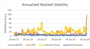
Fig.1: Historical volatilities for various asset classes
Exchange rates (EUR vs USD rates) and interest rates (futures on German Bundesanleihen) exhibit relatively low volatilities of typically below 10%, equities (Standard & Poors 500 index) are typically in the 10-15% range (current extreme levels are due to the massive equity crash).
In contrast, the volatility of power has been in excess of 20% for most of the last 4 years, experiencing periods of well over 30%. Given most financial firms have risk departments for the unique purpose of monitoring risk of assets less volatile than power, at least the same degree of care should be exercised when dealing with power exposures.
Measuring Market Risk with the Historical Simulation Approach
In the downloadable Excel file, we demonstrate the historical simulation approach as an easy-to-use and model-free approach which not only allows to quantify the risk of individual positions, but also enables the measurement of portfolio risk. Using historically observed prices, we demonstrate several basic concepts:Measurement of (log)returns: For purposes of risk measurement we use so-called log-returns (i.e. the natural logarithms of price ratios between dates). A period commonly used for the calculation of VaR is 5 days, based on assuming that 5 days suffice to liquidate a position. Depending on the specific case, different choices may be taken.
Standard deviation of returns: We use the standard deviation of log returns to characterise the breadth of the return distribution. The larger it is, the larger the financial risk of a position.
Cumulative Distribution Function (CDF) and Inverse CDF: By using these functions as shown in the spreadsheet, standard deviations of returns can be turned into P95, P90 etc values. These are loss amounts at different confidence levels, i.e. levels of loss which are not exceeded at defined levels of probability (95%, 90% etc). Congratulations – at this point you have calculated VaR ! What we have derived via the standard deviation of returns and an inverse CDF evaluated at 95% is precisely what practitioners would call a 5d-95% VaR.
Correlation & Portfolio risk: We consider the example of a portfolio of a long position in one contract and a short position in a highly correlated contract (France and Germany). In order to assess the risk of this portfolio, it is sufficient to work out the profits/losses of both positions, to add them up to obtain portfolio profits/losses and to measure the width of the resulting distribution. Visual inspection of the co-dependence of daily logreturns in a scatterplot demonstrates the high degree of correlation which leads to a risk reduction in the portfolio.
While risk measurement methods as used by banks and trading firms may differ in various aspects of the implementation (some use e.g. simulation techniques to generate realisations of returns), the simple examples illustrated on the Excel sheet provide the intuition required to understand much of what risk measurement is all about.
Measuring Credit Risk via Monte Carlo Simulation
In contrast to Market Risk which is driven by only one risk factor (Prices and their dynamics), credit risk is driven by two different risk factors:
Prices: Exposure at Default (EAD) is driven by the price dynamics of PPA contracts in the market. Price volatility leads to differences between initial contract prices, and replacement contract prices prevailing in the market at the time of default.
Counterparty Default: The probability of counterparty default over time is a function of counterparty credit rating and can be simulated separately
By combining the simulation of price dynamics and default events, as shown in below figure, it becomes possible to generate loss scenarios.
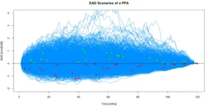
Fig.2: Simulation of credit loss events. Dots indicate individual default events, negative EAD results in losses (red dots), positive EAD means no loss occurs
For an in-depth description of Credit Risk and how to manage it, please take a look at our credit risk article.
COVID-19 and its Impact on PPA Pricing
As the COVID-19 pandemic has hit Europe and countries adopt severe measures to control its further spread, financial markets and energy prices have seen unprecedented shocks.
While lockdowns and factory closures have had massive impacts on current levels of energy consumption, PPA pricing depends on future power prices and their volatility. Here we present some relevant data and elaborate on what implications they may hold for PPA markets going forward.
Lockdowns and Their Impact on Energy Consumption
By mid-March the worst-affected European countries (Italy, France, Spain, Belgium) started to go into lockdown, with immediate consequences for power demand, as can be seen in below graph from Bloomberg New Energy Finance.
The graphs shows colour-coded deviations of demand for power and gas relative to their respective seasonal normal for the months February and March. White means demand levels in line with seasonally expected levels, green indicates higher-than-usual demand and red means lower-than-usual demand.
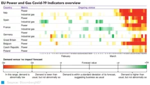
Fig.2: Deviations of power and gas demand from normal seasonal levels
While demand levels were normal for all of February and the beginning of March, rigorous measures were adopted, leading to abnormally low power and gas demand, as is reflected by the red period on the right-hand side of the above figure.
It is also seen that the extent of demand drops depends differs substantially between countries – Germany, where measures were relatively lenient, has seen a relatively modest impact on power & gas consumption.
What Happened to Long-Term Prices
While current demand remains depressed to date, long-term prices are the crucial determinant for the economic viability of merchant renewables. In order to illustrate long-term price impact, below graph shows the evolution of 10yr baseload PPA prices since July 2019.
While early 2020 saw prices slide, dramatic price declines occurred in early March, with the magnitude of daily moves exceeding what was observed after the Fukushima disaster in 2011.
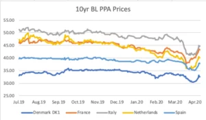
Fig.3: Evolution of 10yr baseload PPA prices since July 2019
Most of the price drops were reversed by early April, and prices have held relatively steady since then. Throughout the drop, term-market liquidity was not disrupted and is now recovering to normal levels again.
Why Does Uncertainty Matter ?
To understand why market price uncertainty affects the pricing of PPAs, we need to take a closer look into how utility offtakers risk-manage PPAs. After entering into a PPA contract, utilities offload the net volume purchased via liquid exchanges and OTC markets.
As they do so, they find liquidity typically in the years 1-3, i.e. they have to “stack up” the entire volume in the contracts they are able to trade (large grey bars). In doing so, they achieve neutrality against parallel moves of the forward curve.
Put differently, if all prices move up or down by the same amount, the net profit/loss impact is zero. However also non-parallel forward curve moves occur, e.g. steepening and flattening of the forward curve.
In these cases, PnL impact is non-zero: Assume a steepening of the forward curve, i.e. long-dated prices appreciate, and short-dated prices depreciate.
In this situation, the long-dated positions acquired via the PPA contract will produce gains on appreciating prices, as will the front-end hedge short positions on dropping prices, i.e. an overall net gain will result.
Analogously, flattening of the curve will give rise to an overall loss. It is this risk component which is proportional to market volatility that utilities cannot hedge. They therefore adjust their pricing by a safety buffer. The size of this safety buffer depends on utilities’ assumption of future volatility.
If they perceive volatility to persist, they will price deals more defensively, those who think volatility will ebb off may choose to transact at more aggressive prices.
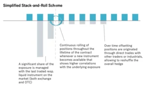
Fig.4: Illustration of the so-called stack-and-roll scheme
Can We Quantify Uncertainty in a Forward – Looking Way ?
The type of analysis we showed in the introductory session on market risk is applicable when we look at past price realisations. However at times where we believe future might look very different from the past, this is clearly not a good approach.
Are there other data sets which could be used to infer expectations on future volatility ? Indeed there are – and they are found in the market for options on power. When traders transact options, they usually express prices in terms of so-called implied volatility.
Implied volatility expresses the expected future volatility level of a contract during the period between the trade date and the date at which the option right can be exercised. The higher it is, the more expensive the option premium.
The key takeaway of this is that we can back out implied volatilites from option premia, and thereby get a picture of market-anticipated volatility. Below figure shows implied volatilities for options on different German power contracts, as currently quoted in the market.
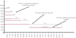
Fig. 5: Implied volatilities for options on different German power contracts. The red line marks the time between quote date and expiry date of the option, the grey line marks the delivery period of the referenced contract.
The immediately visible feature of the graph is that volatilities generally drop as the time until option expiry increases. Very short-term options (e.g. the option on the May’20 baseload contracts) currently trade at extreme volatility levels around 90% vs usual levels of 30-50%.
With increasing time to expiry, this drops, down to a level 31% for the option contract referencing baseload for delivery in 2021. While this is on the high side, historical volatility levels have been in this range several times over the last 4 years, as can be seen in Fig.1.
Finally, the (forward) volatility of the baseload contract for 2022 delivery during 2021 is at ca. 19%, well within the normal historical volatility range.
In other words, the options market implies that markets will remain very choppy in the near term, as COVID-19 related demand uncertainty will likely persist for a while. Based on the data, H2 will see gradually declining volatilities, and volatilities during 2021 are expected to be back in line with a business-as-usual situation.
What is the Takeaway ?
Common wisdom suggests that risk management for renewables is done and dusted once a PPA has been concluded. However, recent events show that risk management may be required at various stages during the life of a project
- Project Delays: Where PPAs have already been concluded, but production go-live dates have to be pushed back due to construction delays or delays in the delivery of equipment, price risk crops up: Irrespective of the reasons for the delay, the delivery obligation under the PPA remains, exposing the project owner to price risk. Fast action needs to be taken to avoid potentially material losses
- Credit Risk: Where offtaker credit ratings are adversely impacted, reassessment of credit risk may be called for. Sizing and structuring credit protection requires carrying out detailed simulations
- Measuring Portfolio Risk : Projects typically use hedging ratios of 70-80%, leaving the remainder of production fully exposed to market risk. For large portfolios across several countries, this may result in material risk positions, calling for sound risk aggregation methodology.
While risk management in power markets has traditionally been the realm of utilities, the complexities of managing risk of renewable assets in merchant regimes point to the urgency of building up competence.
We have prepared an Excel sheet to cover all topics discussed in this article. (See below)
It shows how calculations can be implemented, it lets you play with assumptions in order to see their impact on risk figures, and it helps you build your own spreadsheets to quantify risk.