the Creative Commons Attribution 4.0 License.
the Creative Commons Attribution 4.0 License.
 | 10 Jan 2024
Global 500 m seamless dataset (2000–2022) of land surface reflectance generated from MODIS products
Xiangan Liang
Qiang Liu
Jie Wang
Shuang Chen
Peng Gong
The Moderate Resolution Imaging Spectroradiometer (MODIS) is widely utilized for retrieving land surface reflectance to reflect plant conditions, detect ecosystem phenology, monitor forest fires, and constrain terrestrial energy budgets. However, the state-of-the-art MODIS surface reflectance products suffer from temporal and spatial gaps due to atmospheric conditions (e.g. clouds and aerosols), limiting their use in ecological, agricultural, and environmental studies. Therefore, there is a need for reconstructing spatiotemporally seamless (i.e. gap-filled) surface reflectance data from MODIS products, which is difficult due to the intrinsic inconsistency of observations resulting from various sun/view geometry and the prolonged missing values resulting from polar night or heavy cloud coverage, especially in monsoon season. We built a framework for generating the global 500 m daily seamless data cubes (SDC500) based on MODIS surface reflectance dataset, which contains the generation of a land-cover-based a priori database, bidirectional reflectance distribution function (BRDF) correction, outlier detection, gap filling, and smoothing. The first global spatiotemporally seamless land surface reflectance at 500 m resolution was produced, covering the period from 2000 to 2022. Preliminary evaluation of the dataset at 12 sites worldwide with different land cover demonstrated its robust performance. The quantitative assessment shows that the SDC500 gap-filling results have a root-mean-square error (RMSE) of 0.0496 and a mean absolute error (MAE) of 0.0430. The SDC500 BRDF correction results showed an RMSE of 0.056 and a bias of −0.0085 when compared with MODIS nadir BRDF-adjusted reflectance (NBAR) products, indicating the acceptable accuracy of both products. From a temporal perspective, the SDC500 eliminates abnormal fluctuations while retaining the useful localized feature of rapid disturbances. From a spatial perspective, the SDC500 shows satisfactory spatial continuity. In conclusion, the SDC500 is a well-processed global daily surface reflectance product, which can serve as the fundamental input for large-scale ecological, agricultural, and environmental applications and quantitative remote sensing studies. The SDC500 is available at http://data.starcloud.pcl.ac.cn/resource/27 (Liang et al., 2023b) or https://doi.org/10.12436/SDC500.27.20230701 (Liang et al., 2023a).
- Article
(28519 KB) - Full-text XML
- BibTeX
- EndNote


The increasing global ecological and climatological challenges in recent years have heightened the necessity for a more quantitative understanding of the Earth's system, which demands long-term, high-frequency, and high-quality observation data at a global scale (Estoque, 2020). Optical remote sensing imagery is one of the most widely used data sources for Earth observation. However, about 60 % of pixels in optical remote sensing images are unusable due to cloud cover, dust, and heavy aerosol situations (Claverie et al., 2015; Ju et al., 2012; Vermote et al., 2016), which are usually filled with invalid values or retain their cloudy values. These unusable pixels make the observations spatiotemporally incomplete, hindering their application in studies (Yang et al., 2022; Liu et al., 2021; Fang et al., 2019; Yuan et al., 2011; Liang et al., 2022). Typically, a time-consuming and labour-intensive pre-process is required to fill the spatiotemporal gaps. Therefore, a global, well-processed, spatiotemporally seamless (gap-filled) optical remote sensing observation product is needed to serve as a fundamental input for large-scale applications. For example, the inversion of leaf area index (LAI) and fractional vegetation cover (FVC) parameters in the Global LAnd Surface Satellite (GLASS) product requires gap-filled surface reflectance as input (Tang et al., 2013), and many aerosol estimation algorithms need gap-filled surface reflection to quantify the contribution of the surface reflected radiation component (Yan et al., 2022).
Over the last 2 decades, the MODIS sensors on the Terra and Aqua satellites have provided high-quality global Earth observations at spatial resolutions of 250 m, 500 m, and 1 km (Justice et al., 2002). This makes the MODIS products suitable for generating the global seamless observation data. However, although numerous MODIS reconstruction algorithms are proposed, their practices are mostly applied on the normalized difference vegetation index (NDVI) (Cao et al., 2018; Chu et al., 2021; Li et al., 2023) or other vegetation parameters (Zhu et al., 2013; Cao et al., 2023; Ma et al., 2022; Wild et al., 2022; Ma and Liang, 2022; Chen et al., 2015; Xiao et al., 2016), the research efforts of reconstructing surface reflectance image series are scarce. The land surface reflectance is a fundamental optical remote sensing product, which is derived through atmosphere correction of the top-of-atmosphere reflectance observed by the satellite. As a directly observed physical parameter, the land surface reflectance is widely used to reflect plant conditions (Chen et al., 2019; Fensholt and Proud, 2012), detect ecosystem phenology (Gray et al., 2019; Zhang et al., 2004; Mao et al., 2012), monitor forest disturbance (Lizundia-Loiola et al., 2020), and constrain the terrestrial energy budget (Wu et al., 2017; Jia et al., 2023). Therefore, it is desirable to generate a pre-processed seamless (gap-filled) global land surface reflectance dataset to serve as the primary input for the ecological, agricultural, and environmental applications, as well as for quantitative remote sensing studies (Zhao et al., 2021; Yang et al., 2021; Jiang et al., 2022, 2017; Liu et al., 2012).
Generally, there are two main challenges in reconstructing the seamless MODIS land surface reflectance data.
First, the intrinsic inconsistency of observations due to various sun/view geometries. In contrast to vegetation parameters such as NDVI and LAI, the land surface reflectance is affected by the surface bidirectional reflectance distribution function (BRDF). This creates an artificial variance in the surface reflectance time series as the observations of a specific pixels on different dates correspond to different sun/view angles. Although the BRDF effect can be useful in quantitative retrievals of surface albedo and canopy architecture parameters, it is typically considered to be noise and is preferably removed in most applications. The MODIS nadir BRDF-adjusted reflectance (NBAR) dataset (MCD43A4) was generated from the BRDF correction of the original MODIS land surface reflectance product (MOD09GA) for the purpose of vegetation monitoring and phenological studies (Schaaf et al., 2012, 2002). However, as the BRDF inversion model of the NBAR dataset requires the cumulation of multiple clear observations in a 16 d window, the resulting NBAR dataset still suffers from missing data. Additionally, although the ideal surface reflectance should be corrected for atmospheric effects, the actual MODIS surface reflectance product (MOD09GA) still suffers from the residual influence of cloud and aerosols, which bring further discontinuity into the observation data. Tang et al. (2013) used the temporal smoothing method to reduce the intrinsic inconsistency of MODIS surface reflectance series and to improve the cloud detection results. However, their method did not consider the BRDF effect, which increased the uncertainty in the cloud detection and smoothing. There is also research aimed at the generation of seamless NBAR images (Sun et al., 2017; Ju et al., 2010); their algorithms are entangled with the BRDF inversion and become complex, which may be the reason that a global and long-term seamless dataset has not been published till now. In this paper, a land-cover-based BRDF correction is adopted to normalize the surface reflectance product before smoothing out the time series.
Second, while a large number of gap-filling methods have been proposed, the challenge of prolonged continuous missing values resulting from heavy cloud coverage during the monsoon season or polar night has not been addressed well. It is essential to have a robust algorithm to fill the long gaps in time series of observations. Typically, mathematical filters such as rolling-average or Savitzky–Golay (SG) filters are often employed to smooth out the time series of observations (Chen et al., 2004), as well as to fill gaps (Zhao et al., 2009). However, in many regions worldwide, there exist prolonged continuous missing observations resulting from heavy cloud cover during the rainy season (e.g. in the Amazon, central Africa, and southern and southeastern Asia) or due to polar nights (e.g. in the Antarctic and sub-Arctic region). The limited window length of rolling-average or SG filters makes them incapable of dealing with data containing long gaps (Kawala-Sterniuk et al., 2020). Other approaches using frequency domain filters to process remote sensing time series have also been proposed (Yang et al., 2015; Zhou et al., 2015). For example, the penalized least-square regression based on the discrete cosine transform (DCT-PLS) method has been applied to generate continuous surface reflectance series from MODIS products (Xiao et al., 2015), as well as Sentinel-2 Multi-Spectral Imagery (MSI) images (Yang et al., 2022). Although a frequency domain filter can leverage the periodicity in multi-annual data for time series reconstruction (i.e. the rainy season or polar night occur during the same season of the year), the information for filling these gaps is still lacking, making the results questionable. Another set of algorithms fills long gaps based on a priori information, which is generally derived from statistics of the parameter in ground measurement or satellite products (Liu et al., 2017). For instance, Moody et al. (2005) first proposed the ecosystem curve-fitting algorithm to construct a spatially seamless albedo dataset based on the assumption that pixels of the same ecosystem class should exhibit similar phenological behavioural curves. This methodology was later improved for LAI gap filling (Fang et al., 2008) and was also adopted to generate the global seamless GLASS albedo product (Liu et al., 2013). A newer study used a similar method to fill gaps in NDVI series before applying the SG filter (Chen et al., 2021). However, the gap-filling method based on a priori information has only been applied for vegetation-related parameters. Its potential for filling gaps in surface reflectance is yet to be explored. In this paper, a land-cover-based a priori database is established to aid the gap-filling process.
The aim of this study is to generate the first global spatiotemporally seamless land surface reflectance at a resolution of 500 m (SDC500) based on MODIS products, covering the period from 2000 to 2022. An advanced framework was proposed to address the two main challenges of reconstructing MODIS land surface reflectance data, including land-cover-based a priori database establishment, BRDF correction, outlier detection, gap filling, and slide window smoothing. Quantitative validations were conducted on the proposed gap-filling and BRDF correction methods. Furthermore, the performance of SDC500 was assessed at 12 sites worldwide with different land covers.
2.1 MODIS surface reflectance products MOD09GA (version 6.1) and MYD09A1 (version 6.1)
The MOD09GA product is a daily surface reflectance dataset with a 500 m spatial resolution obtained from the morning satellite EOS-terra (Barnes et al., 1998; Vermote et al., 2011). It contains a quality band that indicates whether the pixel is affected by snow, cloud, or cloud shadow. The MOD09GA dataset is the fundamental input data of SDC500, and cloud-contaminated pixels were removed in the pre-processing stage. The MYD09A1 dataset provides 8 d surface reflectance at a 500 m spatial resolution, acquired by the afternoon satellite EOS-aqua. Each pixel of MYD09A1 contains the best observation among the 8 d. Both the MOD09GA and MYD09A1 data were accessed from the Land Processes Distributed Active Archive Center: https://lpdaac.usgs.gov (last access: 15 August 2023).
2.2 MODIS land cover product MCD12Q1 (version 6.1)
MCD12Q1 is a MODIS land cover product that combines the observations from both EOS-terra and EOS-aqua (Sulla-Menashe and Friedl, 2018; Friedl et al., 2002). It adopts the International Geosphere–Biosphere Programme (IGBP) land cover classification system, which divides the global land surface into 16 ecosystems. In this paper, MCD12Q1 is adopted when building the a priori database for BRDF parameters for different land cover types.
2.3 MODIS BRDF parameter product MCD43A1 (version 6.1)
The MODIS BRDF parameter product MCD43A1 is currently the most widely used and acknowledge remote sensing BRDF dataset (Schaaf et al., 2002, 2012), providing three BRDF kernel model parameters, fiso, fvol, and fgeo, with a spatial resolution of 500 m, which can be used for BRDF correction. The MCD43A1 product is adopted for generating the parameters for BRDF correction, and it can be easily accessed and processed through the Google Earth Engine (GEE) platform.
2.4 MODIS nadir BRDF-adjusted reflectance product MCD43A4 (version 6.1)
The MODIS nadir BRDF-adjusted reflectance (NBAR) product MCD43A4 is generated to facilitate vegetation monitoring and phenological studies, in which the MOD09 surface reflectance data are corrected to nadir-viewing angles using images in a 16 d sliding widow (Schaaf et al., 2002; Vermote et al., 1997). However, as the inversion of the BRDF model needs the cumulation of multiple clear observations in a 16 d window, the resulting NBAR dataset suffers from missing data and is limited in its applications. The MODIS NBAR product (MCD43A4) is chosen for a comparison with our BRDF-corrected results because it is also derived from MODIS data and also normalized to a standard sun/view geometry.
The study aims to reconstruct the time series of MODIS observations in a pixel-based way. The daily observations acquired by morning satellite EOS-terra, i.e. the MOD09GA product, is the major input data. And the 8 d observations acquired by the afternoon satellite EOS-aqua, i.e. the MYD09A1 product, serve as supplemental input data, which are used only when the MOD09GA pixel is marked as cloud contaminated and when the MYD09A1 pixel is marked as clear. The purpose of the differentiated treatments of EOS-terra and EOS-aqua is to make the results more like morning observation and thus more compatible with high-resolution satellite data such as Landsat and Sentinel series, while a small part of afternoon clear observations can help to stabilize the algorithm in case all the morning observations were contaminated by cloud.
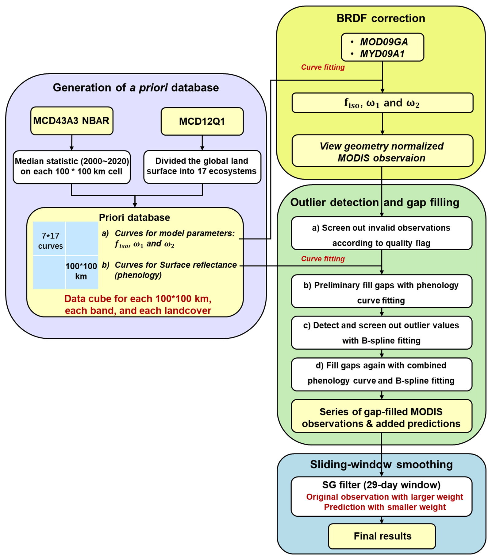
Figure 1 illustrates the three main modules involved in this process: (1) land-cover-based BRDF correction, (2) outlier detection and gap filling, and (3) sliding-window smoothing. The primary challenge in this study is to account for the uncertainty that arises from BRDF effects and cloud contamination. A priori information plays a crucial role in the reconstruction algorithm by providing knowledge of BRDF and phenology. Since both the BRDF correction and gap-filling functions depend on a priori information, we will first introduce the process to generate the a priori database.
3.1 Generation of the a priori database
The MODIS BRDF product MCD43A3 is adopted to generate the a priori database for BRDF and phenology as it is currently the most widely used and acknowledged remote sensing BRDF dataset. Directly using the MCD43A3 dataset in a per-pixel and per-date way is not practical due to the presence of noise and missing values. So, we derive robust statistics from the MCD43A3 dataset and utilize them for BRDF correction.
The following formula expresses the kernel-driven RossThick-LiSparse-Reciprocal (RTLSR) model:
where and are two kernel functions representing volumetric scattering and geometric–optical-shadowing effects, respectively; fiso, fvol, and fgeo are the three model parameters, which constitute the main content in the MCD43A3 dataset.
Before doing the statistics, we apply a simple transform:
where ω1 and ω2 are called BRDF shape factors. They jointly decide the shape of the angular variation of the BRDF model which will be applied to the BRDF correction in the next section.
Land surface classification is also considered in building the a priori database. The MODIS land cover type product MCD12Q1 is adopted for this purpose, and the IGBP land cover classification system within the MCD12Q1 product is adopted, which divided the global land surface into 16 ecosystems.
The cloud computing platform of the Google Earth Engine (GEE) has enabled us to efficiently access and process the large global MCD43A3 and MCD12Q1 datasets. The statistics are derived by computing the median values of fiso, ω1, and ω2 for each MODIS land band, every 4 Julian days, and each land cover type for spatial cells of 100 km × 100 km with a grid space of 50 km. The time scope is from 2000 to 2021, and the spatial extent includes all land surfaces, as well as shallow seas covered by the MCD43A3 dataset. The median statistics are chosen for their resistance to noise, and the coarse spatial resolution ensures an ample sample size of MCD43A3 pixels. However, not all land cover types have valid median statistics in each spatiotemporal cell. For example, a cell in the tropical desert may not have any snow, cropland, or forest samples. In these cases, we filled the missing statistics with the average of neighbouring valid statistics and iterated the filling process until all spatiotemporal cells contained statistics for all land cover types. This process enabled us to generate a global a priori database for BRDF and phenology. The GEE code can be accessed at https://code.earthengine.google.com/363b4d94090048f9e28103ad3efebfdf (last access: 15 October 2023).
3.2 Land-cover-based BRDF correction
To utilize the a priori information on BRDF and phenology, the first step is to select one sequence of time series of fiso, ω1, and ω2 from the a priori database. For each input MODIS pixel, we use the coordinate of the 500 m pixel in the MODIS projection grid to locate the nearest time series of 100 km × 100 km statistics, which corresponds to each of the 17 land cover types. We use the 500 m resolution land cover product MCD12Q1 to acquire the cover type of the pixel. In consideration of ambiguous classifications or mixed pixels, we also select several alternative cover types. For example, if the pixel is indicated as evergreen needleleaf forest in the MCD12Q1 product then evergreen broadleaf forest, deciduous needleleaf forest, mixed forests, and closed shrubland are candidates for alternative cover. The a priori statistics of fiso, ω1, and ω2 for these several possible cover types are used to simulate the candidate sequences of time series according to the actual observation date and sun/view geometry. We then compute the correlation coefficient between the actual MODIS observation and the several simulated candidate sequences. The candidate sequence of fiso, ω1, and ω2, which corresponds to the maximum correlation coefficient, is selected for the following BRDF correction.
The process of BRDF correction is also known as BRDF normalization. As MODIS is a wide-angle sensor, the sun/view angle of a pixel varies from day to day, resulting in fluctuations in the observed time series of the surface reflectance. The objective of BRDF normalization is to simulate a time series that appears as if it was taken from standardized sun/view angles. In this approach, the standardized sun/view angles are defined as nadir viewing and solar illuminating at 10:30 am local time, which is denoted as . Then, the normalization is performed with the following formula:
in which the ω1 and ω1 are derived from the a priori information.
3.3 Outlier detection and gap filling
In this study, the gap refers to both the unobserved area of land surface in the daily MODIS acquisition and the area blocked by cloud or heavy aerosols. These gaps need to be filled with a prediction model to build the seamless dataset. Pure mathematical algorithms, such as linear or nonlinear interpolation, can be efficient prediction models when good-quality, valid samples are available near the gap. However, filling the prolonged continuous gaps and gaps with high levels of noise existing in nearby valid samples can be challenging. In these cases, the ecosystem curve-fitting method is the most robust gap-filling algorithm because it utilized the a priori information of phenology. Therefore, we have designed a strategy that combines the mathematical and the phenology curve-fitting algorithms, as illustrated in the second box of Fig. 1.
Step (a) first excludes the invalid observations according to the quality flag in MOD09GA. Then, step (b) provides preliminary fill values with phenology fitting to increase the stability and error resistance of the gap-filling process. As the phenology fitting is more stable and less flexible than the B-spline fitting, we apply it to provide preliminary fill values which will be utilized in the B-spline fitting step to prevent overfitting. And in step (c) of B-spline fitting, the observations with a fitting absolute error larger than 2.5 times the mean are marked as outliers, which usually means undetected cloud contamination or abnormal change of surface state such as ephemeral snow. These outlier values severely destabilize the fitting process and increase error. Therefore, in this study, we remove the outliers from the observation series together with invalid values indicated by the quality flag in the MOD09GA dataset.
The phenology fitting of step (b) can be expressed as the optimization of the following expression:
where Fphe(t) is the a priori phenology curve, which is actually the series of fiso selected in Sect. 2.2; y1(t) refers to the preliminary prediction values for the time series; a0 and a1 are parameters to be optimized by the least-squares principle, which minimizes the square error between predictions and valid observations in the time series.
The B-spline of step (c) can be expressed as the optimization of the following expression:
where y2(t) is the prediction by spline; are six B-spline base functions; and are seven parameters to be optimized by the least-squares principle. In this step, the preliminary prediction values are included in the samples together with the valid observations, and the outliers are detected and removed in an iterative way.
In the last step, the combined spline and phenology curve fitting of step (d) is expressed as follows:
In this step, the prediction values by spline from step (c) are included in the samples, and there is no outlier detection iteration. The six B-spline base functions, as well as a demonstration phenology curve, are illustrated in Fig. 2. The demonstration phenology curve is in a red band (MODIS band 1) corresponding to a cropland pixel in the North China Plain.
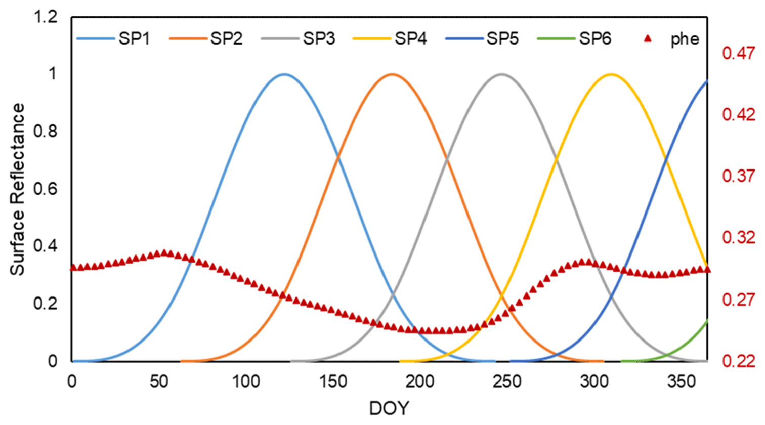
Figure 2Illustration of the B-spline base functions (SP1,…, SP6) and the surface reflectance phenology curve (PHE) of MODIS band 1.
3.4 Sliding-window smoothing
The gap-filling process produces a time series that includes both actual MODIS observations and predicted filling values. However, this series is not completely smooth due to noise in the observations and inconsistency between the two groups. To ensure that the dataset is smooth, we applied the SG filter algorithm (Chen et al., 2004) to the gap-filled series. This algorithm applies a filter window of 29 d in width, which is centred on each output date and slides through the time series. The algorithm also gives larger weight to the actual MODIS observations than the predicted filling values to ensure that the resulting time series remains as close to the original observations as possible.
3.5 Consideration of snow
The time series processing described above is based on the assumption that surface reflectance changes gradually over time, which is not always the case for natural land surfaces. Abrupt changes, such as snowfall, can result in an abrupt change in surface reflectance, and the melting of snow can also cause rapid changes that cannot be simulated with B-spline and phenology curves. Furthermore, the BRDF feature of snow is completely different from that of snow-free surfaces. To address these issues, a special treatment for snow was developed.
The year is divided into two parts, the snow season and the snow-free season, based on the snow indicator in the quality flag of the MOD09GA product. To ensure a robust segmentation, a median filter with a length of 12 d is applied to the snow indicator series. If there are no valid observations within the range of the median filter, the resulting snow status is copied from the nearest valid neighbour.
The BRDF correction, gap-filling, and smoothing processes are then separately applied to the snow season and snow-free season of the time series. During the processing of the snow season, only the observations marked as snow are used to build a smooth snow reflectance curve and vice versa. Finally, the smooth snow reflectance curve and smooth snow-free reflectance curve are combined to create the final time series of surface reflectance. As a result, the final time series may be discontinuous in the switching date from snow season to snow-free season.
The proposed framework has been utilized to generate the SDC500, a global seamless data cube, from the MODIS land surface reflectance dataset. The SDC500 encompasses all land surfaces worldwide, including shallow sea areas, and covers the temporal period from 2000 to 2022. It exhibits a spatial resolution of 500 m and a temporal resolution of 1 d. The SDC500 comprises eight bands, with the first seven bands representing surface reflectance in the MODIS band 1 to band 7 and with the eighth band serving as a quality assessment (QA) band.
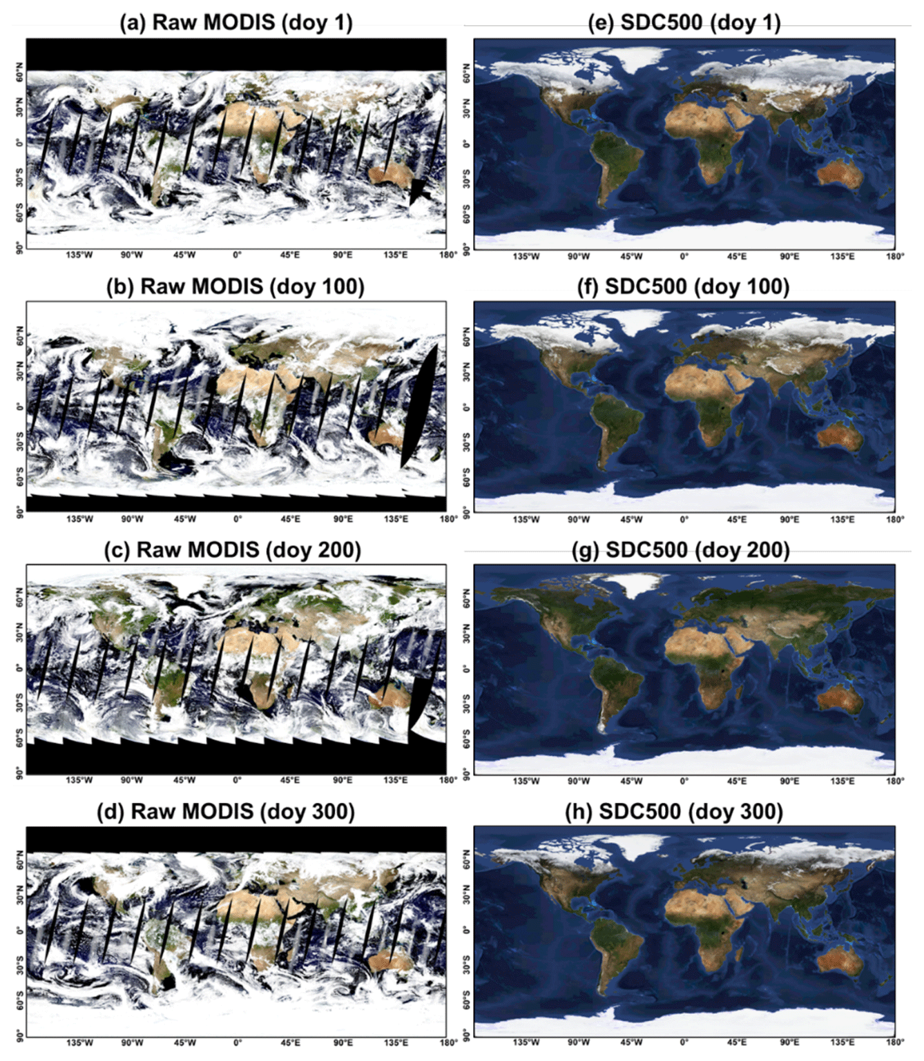
Figure 3True-colour composite (red: band 1; green: band 4; blue: band 3) imageries of raw MODIS observations (a–d) and SDC500 (e–h) for different seasons in 2020.
We present a joint visualization of the SDC500 and raw MOD09GA data for 4 specific days in 2020, resulting in real-colour composite maps at a global scale (Fig. 3). The comparison between the SDC500 and raw data highlights the accurate reconstruction of missing or cloud-covered pixel values by the SDC500. Furthermore, the SDC500 effectively suppresses noise caused by observational conditions and corrects biased pixel values. The reconstructed SDC500 exhibits impressive spatial continuity, indicating its potential and readiness to support a wide range of applications.
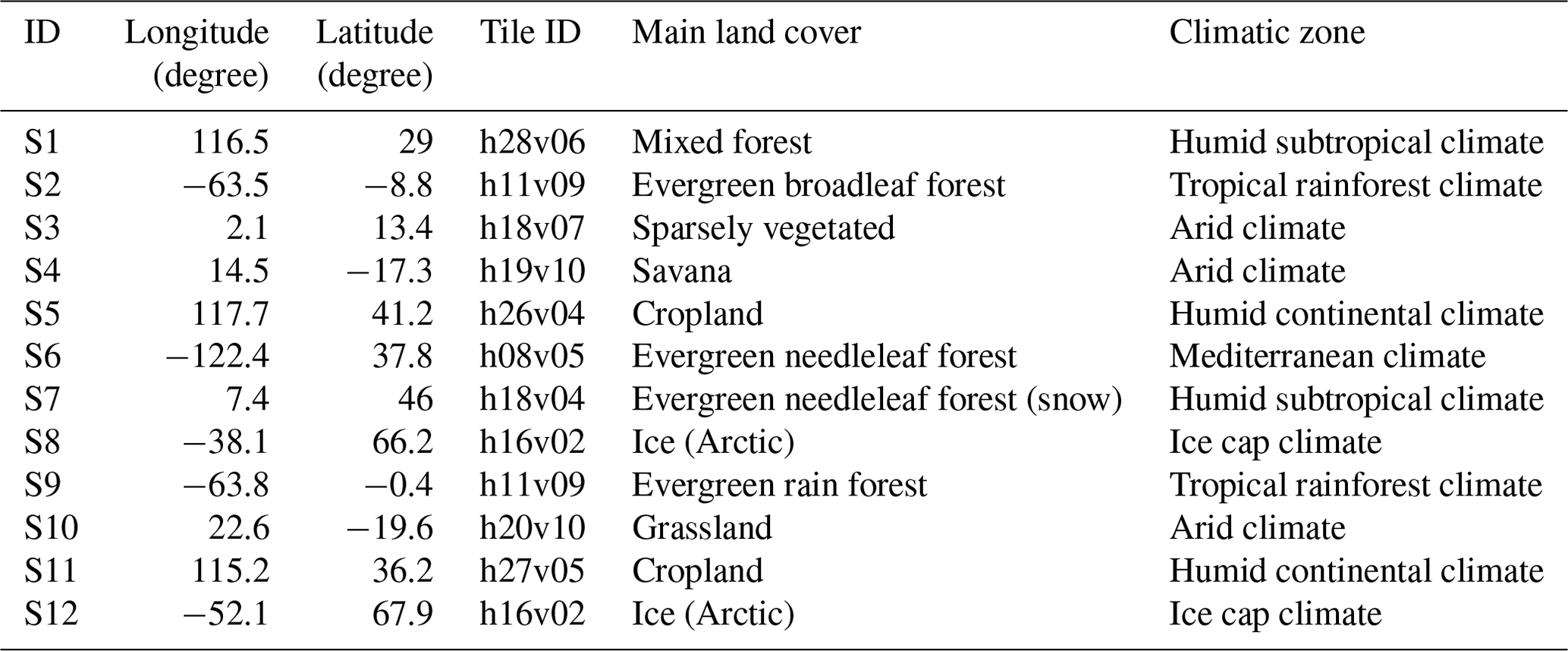
To demonstrate the performance of our algorithms, we selected 12 typical sites distributed around the globe to evaluate the quality of SDC500 (Fig. 4). Sites S1–S8 are selected to visually investigate the spatial pattern, as well as the time series profile of the reconstructed results under different climatic conditions. These sites can be grouped into four categories: sites S1 and S2 represent the case of tropical and subtropical monsoon climate zones, where vegetation is dense and cloud coverage presents the main challenge to remote sensing applications. Sites S3 and S4 represent the case of acrid areas where vegetation is sparse but can change significantly after occasional precipitation. Sites S5 and S6 represent the vegetated area in the temperate climate where crop rotation and natural plant phenology are usually the focus of remote sensing applications. Sites S7 and S8 are in high latitudes or high altitudes, where snow covers the ground for most of the year. Thus, the surface reflectance is generally high, and the snow and/or thaw processes shape the variation of surface status. Sites S9–S12 are selected for visualizing the results of each step of the processing algorithm in the proposed SDC500 framework. In the following section, we first visualized each step of the processing algorithm in Sect. 4.1, then we presented the image blocks of 200×200 pixels in Sect. 4.2–4.5.
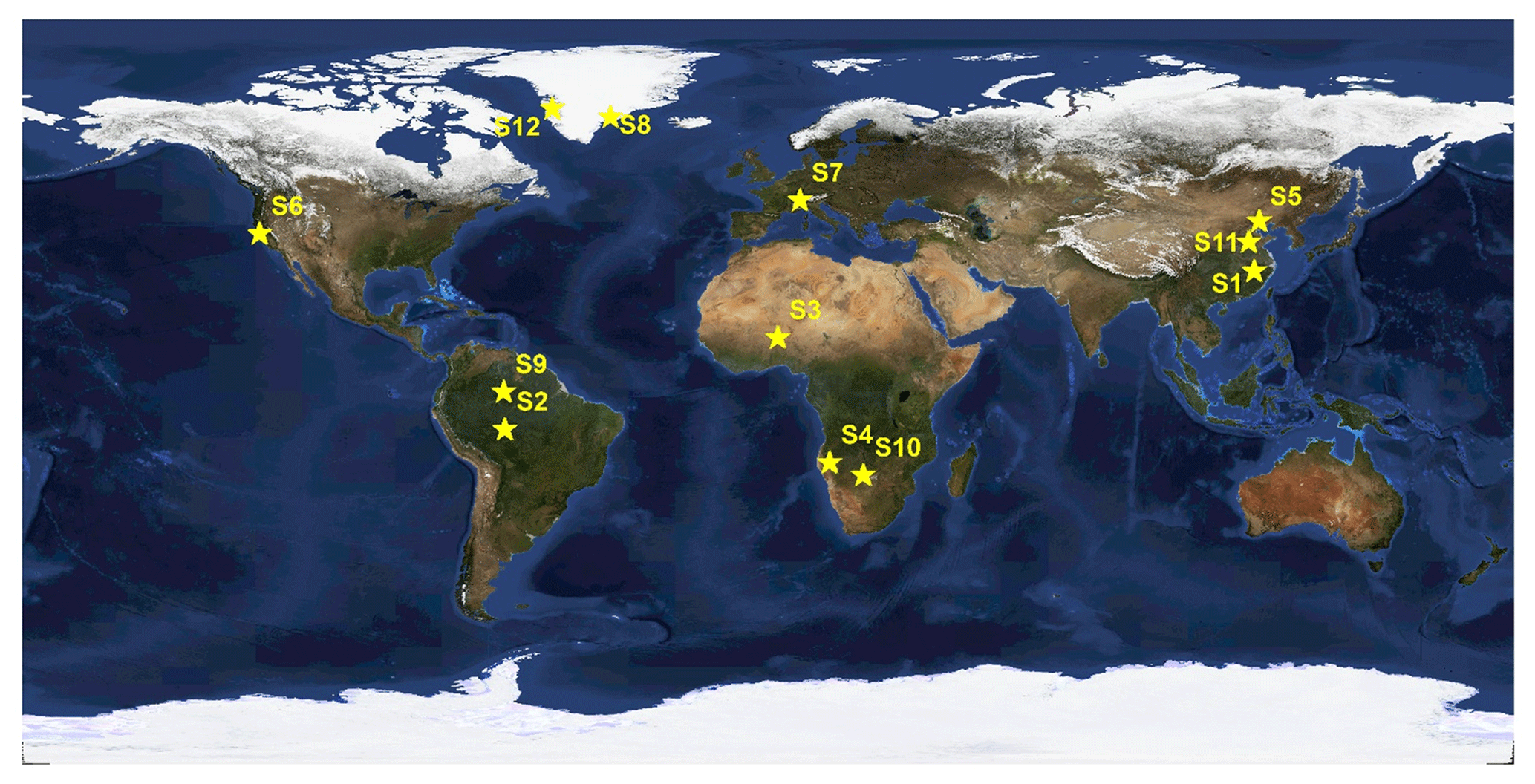
Figure 4Spatial distribution of the 12 validation sites.
4.1 Visualizing each step in the SDC500 processing
We selected temporal curves of four representative sites to evaluate the effect of each step in the proposed framework, respectively. Figure 5 presents band-2 (NIR) reflectance time series in four representative sites in 2010. The original MODIS sensor observations, the outlier detection and gap-filled curve, the first smoothing results, and the final SDC500 results are shown together to facilitate visual validation.
Site S9 (Fig. 5a) is located in the Amazon Plain in Brazil, representing evergreen forest land cover, as well as a case of scarce clear observation. We can see that, in Site S9, the first gap-filling result by phenology curve (green dash-dot line) is too flat as the a priori phenology curve has a in coarse resolution and lacks details. However, the final SDC500 (red line) effectively reflects the seasonal dynamic while avoiding over-fitting, giving a reasonable result in the tropical zone.
Site S10 (Fig. 5b) is located in the southern part of Africa, representing grassland in the wet season and sparsely vegetated surfaces in the dry season. In Site 10, clear observations are dense, and the reconstruction results are close to the unbiased average status of the surface.
Site S11 (Fig. 5c) is located in the temperate zone of the North China Plain, where winter wheat grows from October to June and where corn grows from July to September. The discrete series (orange cross) of Site S11 show double peaks in summer around DOY 130 and 220 and three valleys around DOY 50, 190, and 300. We can see that the first gap filling (green dash-dot line) cannot approximate the double peak feature of the crop phenology, but the second gap filling (grey line) and the final smoothing (red line) gradually approach the discrete series (cross). It illustrates that SDC500 has stable estimation capabilities near peak and valley values.
Site S12 (Fig. 5d) is located in the sub-Arctic coastal land of Greenland and is featured for the snow–thaw circle and long polar nights in winter. In Site S12, the reconstructed result (red line) is composed of two parts: the snow-free part (140 < DOY < 305) with low reflectance and the snow-covered part with high reflectance. In the DOY range of 280–300, there are some large fluctuations in the raw observations (orange cross); a small part of the observations is marked as snow covered, and the rest is marked as snow free according to the raw quality flag. Our algorithm judges this period to be more snow free according to the median filter so the final reconstructed result (red line) is closer to the lower envelope of raw observations. In the data range before DOY 50 and after DOY 300, the site enters the polar night, and there is no valid raw observation (orange cross). The prediction in the polar night may not be as accurate as the normal date, but the reconstructed result (red line) still gives a reasonable prediction.
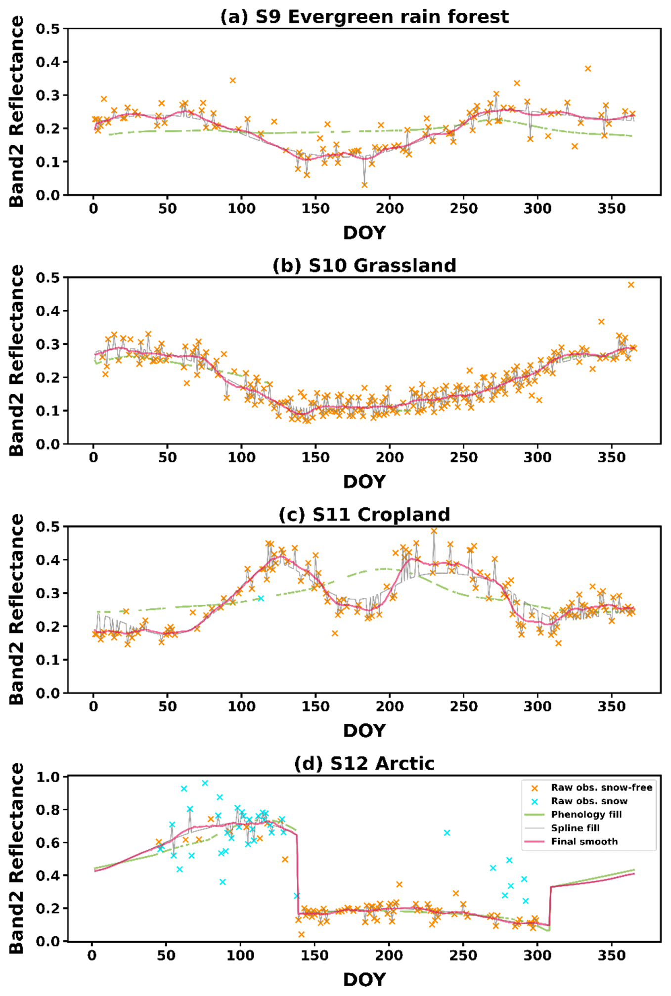
Figure 5Comparison of BRDF-adjusted raw MODIS observations, gap filled values with the phenology curve, gap-filled values with the B-spline + raw observations, and the final smoothed series in typical sites: Site S9 evergreen rain forest (a), Site S10 grassland (b), Site S11 cropland (c), and Site S12 arctic (d).
4.2 SDC500 in tropical and subtropical areas
In the tropical and subtropical monsoon climate zones (Figs. 6 and 7), heavy cloud cover significantly affects the satellite observations. Particularly during the monsoon season from May to August, there is continuous and dense cloud coverage, leading to prolonged gaps in valid observations. This poses a considerable challenge for seamless observation reconstruction. Simple linear interpolation performs poorly due to the extensive missing data. But SDC500 can effectively fill these prolonged gaps and reconstructs observation time series that closely reflect the actual conditions.
From a spatial patterns perspective, the reconstructed results of SDC500 demonstrate the preservation of effective observation values in the central cloud-free area in site S1 on DOY 226 compared to the original observations (Fig. 6b). Additionally, the reconstructed data in cloud-covered areas exhibit good spatial consistency with the raw MODIS data in cloud-free areas. This spatial consistency is particularly notable considering that the SDC500 is constructed on a pixel-wise basis. It indicates the reliability of the reconstruction algorithm.
From the temporal series perspective, despite significant cloud interference and numerous data gaps before and after this period, SDC500 successfully reconstructs the missing data and preserves the phenological characteristics of forests, as illustrated in Fig. 6a. In site S2 (Fig. 7a), which is mainly covered by evergreen broadleaf forest, reflectance remains relatively stable throughout the year, and SDC500 effectively eliminates noises and obtains stable phenological curves.
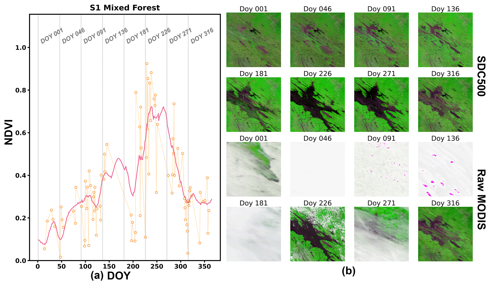
Figure 6Performance of SDC in site S1. (a) The NDVI curves for the central pixel; the orange points indicate the valid MODIS observations, and the red line indicates the SDC500 results. (b) The spatial pattern of reconstructed and raw image blocks of 200×200 pixels centred around the site (red: band 1, green: band 2, and blue: band 3).
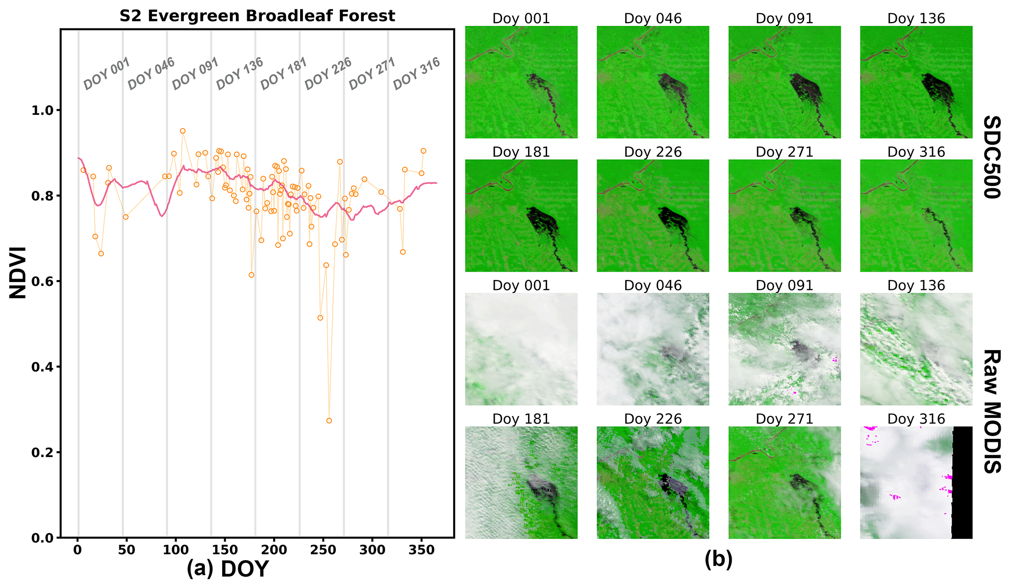
Figure 7Performance of SDC in site S2. (a) The NDVI curves for the central pixel; the orange points indicate the valid MODIS observations, and the red line indicates the SDC500 results. (b) The spatial pattern of image blocks of 200×200 pixels centred around the site (red: band 1, green: band 2, and blue: band 3).
4.3 SDC500 in acrid areas
The SDC500 demonstrates excellent noise reduction performance in the acrid area (Figs. 8 and 9). Figure 8b illustrates that the raw MODIS observation on DOY 091 is affected by its large view angle, resulting in no data in the main part of the block, and the remaining upper-left corner is brighter than other raw images. However, these are effectively corrected in the SDC500 reconstructed results, which show consistency with observations on other days. The improved observation consistency on different dates mitigates the inherent data inconsistency arising from sensor component fluctuations, observation/view geometry, and other factors. Notably, in Fig. 9b, the reflectance of water bodies in the images remains consistent throughout the year, without any noticeable darkening or lightening, aligning closely with the physical reality. From the temporal perspective, the NDVI series in S3 (Fig. 8b) peaks at about DOY 250, while the NDVI series in S4 (Fig. 9b) peaks at about DOY 50, which is consistent with the fact that the two sites are in different hemispheres. Additionally, the influence of outlier values has been satisfactorily removed, such as around DOY 200 and 250 in Fig. 8a.
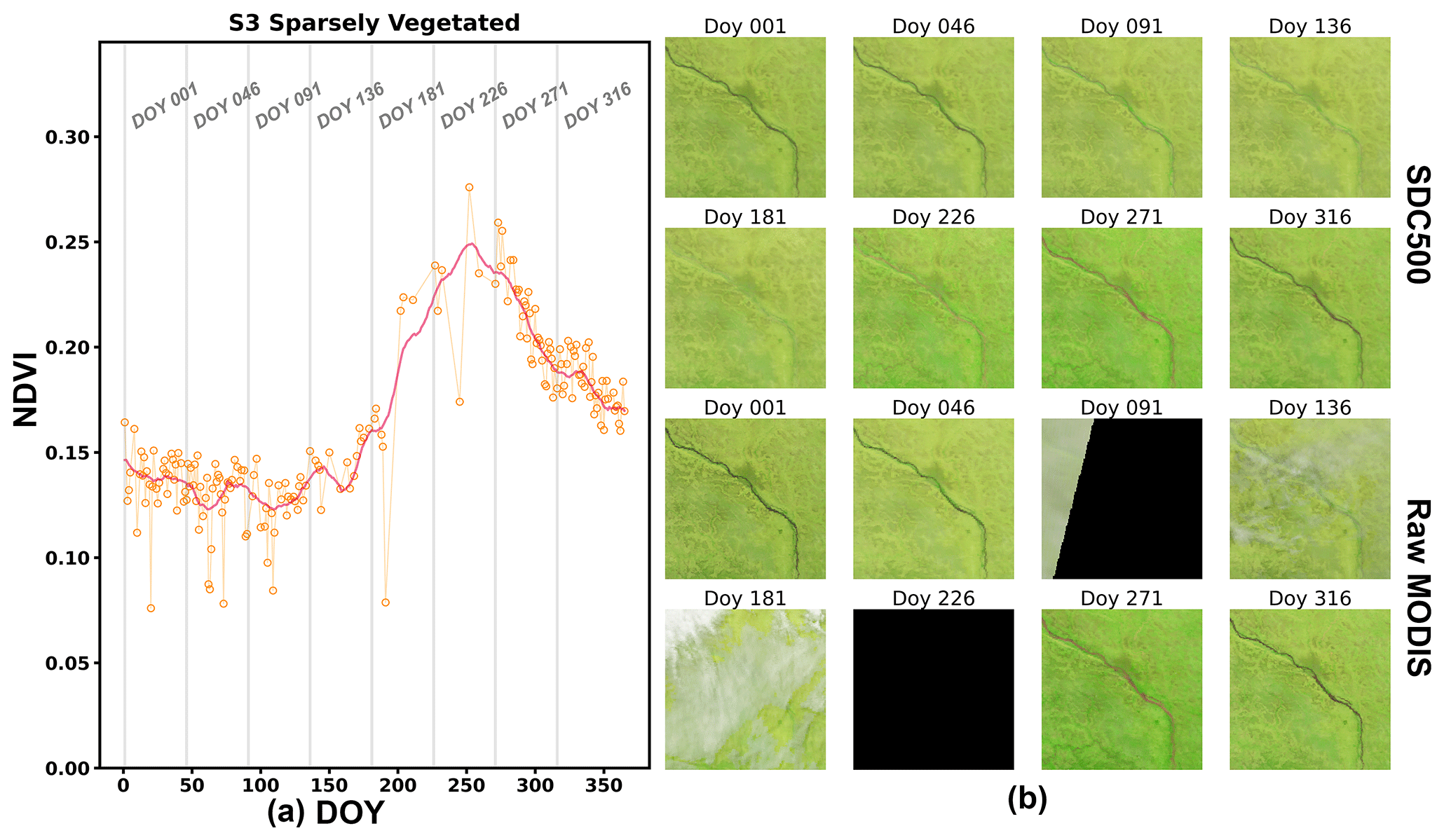
Figure 8Performance of SDC in site S3. (a) The NDVI curves for the central pixel; the orange points indicate the valid MODIS observations, and the red line indicates the SDC500 results. (b) The spatial pattern of image blocks of 200×200 pixels centred around the site (red: band 1, green: band 2, and blue: band 3).
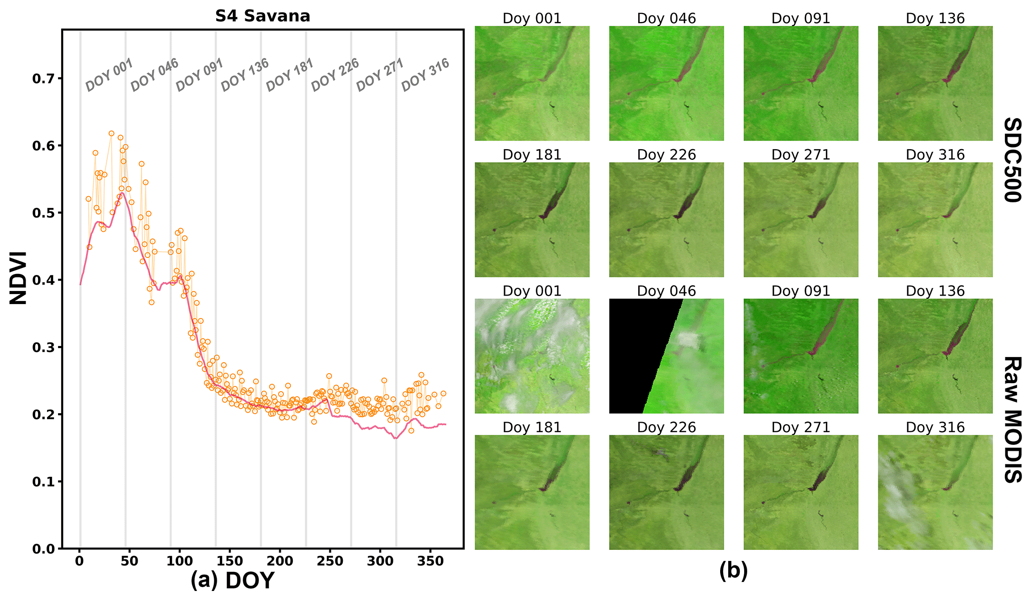
Figure 9Performance of SDC in site S4. (a) The NDVI curves for the central pixel; the orange points indicate the valid MODIS observations, and the red line indicates the SDC500 results. (b) The spatial pattern of image blocks of 200×200 pixels centred around the site (red: band 1, green: band 2, and blue: band 3).
4.4 SDC500 in temperate-climate areas
The primary land cover type of site S5 (Fig. 10) is cropland, which thrives in summer and is harvested in autumn each year. Hence, the typical NDVI phenology of cropland can be used as a reference to assess the performance of SDC500. In this evaluation, we assume that the NDVI phenologies in neighbouring years are similar for most of the pixels in the image block. Therefore, comparing the NDVI patterns over 2 years allows us to gauge the credibility of the reconstructed image. The comparison of SDC500 and raw NDVI images for the same day in 2020 and 2021 is presented in Figs. 11 and 12. The reconstructed NDVI series in Fig. 11 exhibits a transition from low to high and then back to low in the DOY range 110–310 in 2020, which aligns with the temporal curve pattern observed in 2021. Consequently, the NDVI values for the same day in different years are comparable. For example, DOY 110 in 2021 (second line in Fig. 13) is relatively cloud free and can be considered to be reliable in terms of reference data. The reconstructed NDVI image for DOY 110 in 2020 (third line in Fig. 12) agrees well with that of DOY 110 in 2021, indicating the accuracy of the reconstructed result. Similarly, DOY 260 in 2021 (second line in Fig. 13) can serve as reference data to validate the reconstructed result of DOY 260 in 2020 (third line in Fig. 12). Furthermore, certain parts of the region on DOY 160 and 310 in 2020 (second line in Fig. 12) are not affected by clouds and can be used as reference data. The reconstructed results on DOY 160 and 310 in 2021 (3rd line in Fig. 13) effectively preserve the high-quality observations in these regions, exhibiting good spatial continuity with the reconstructed results in cloud-contaminated regions. As the SDC500 is produced on a per-pixel basis, the consistency between clear and cloud-contaminated pixels demonstrates the robustness of the algorithm. Additionally, the results reveal the successful restoration of low NDVI values caused by clouds while preserving the low NDVI values of bare-land roads. This indicates the successful reconstruction of spatiotemporally continuous missing pixels by the proposed algorithm.
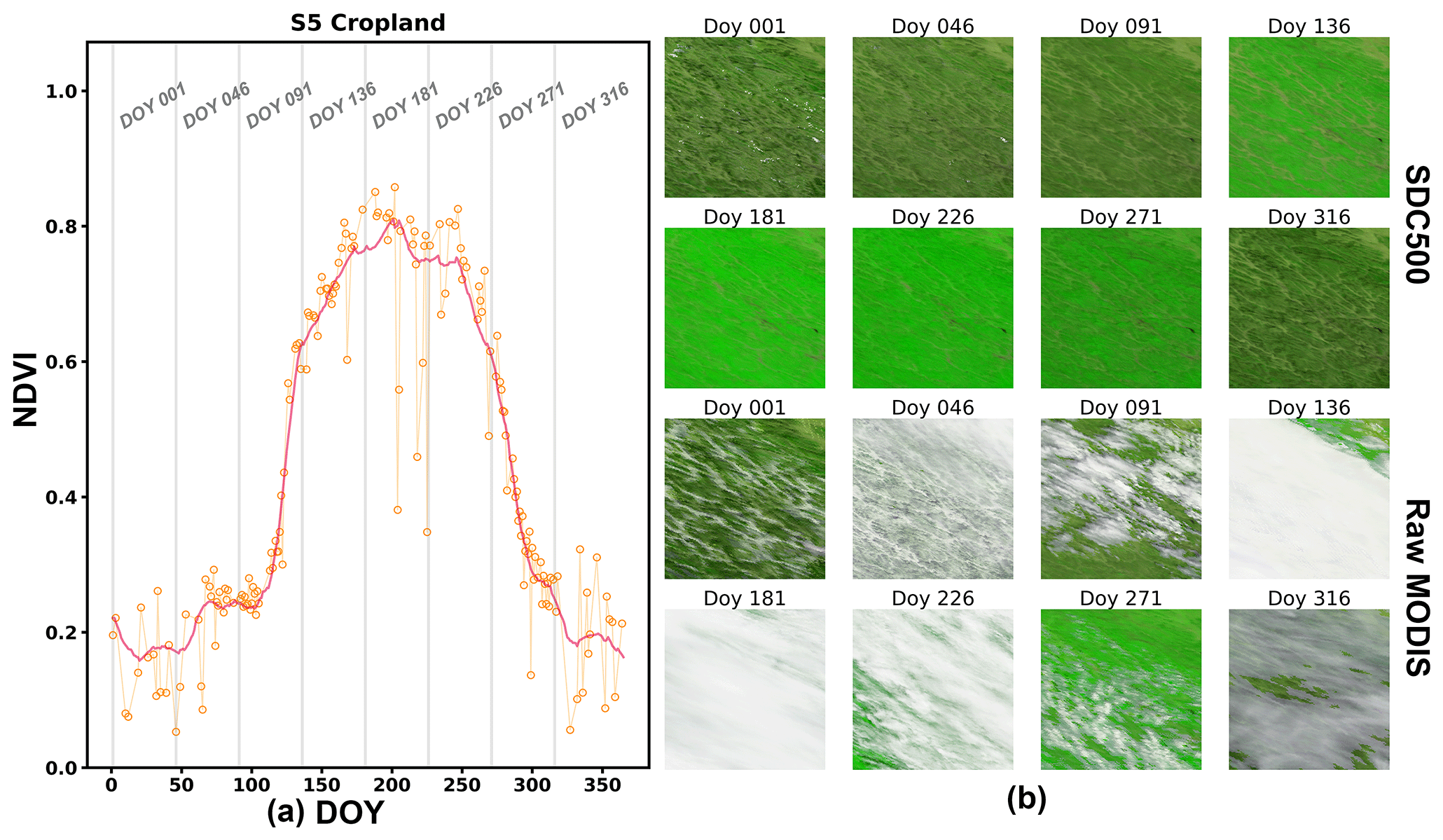
Figure 10Performance of SDC in site S5. (a) The NDVI curves for the central pixel; the orange points indicate the valid MODIS observations, and the red line indicates the SDC500 results. (b) The spatial pattern of image blocks of 200×200 pixels centred around the site (red: band 1, green: band 2, and blue: Band 3).
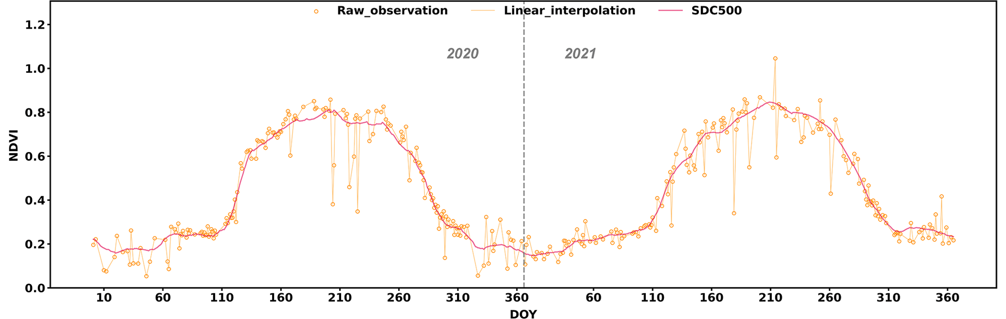
Figure 11NDVI curves of the central pixel in a cropland area (site S5) in the period of 2020 and 2021.
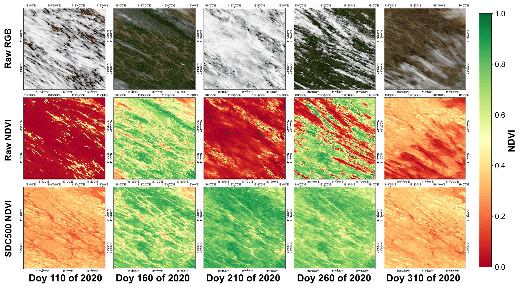
Figure 12Assessment of spatial pattern in a cropland area (site S5). True-colour composite (red: band 1, green: band 4, and blue: band 3) and raw MODIS NDVI and SDC500 NDVI imageries on five dates in 2020.
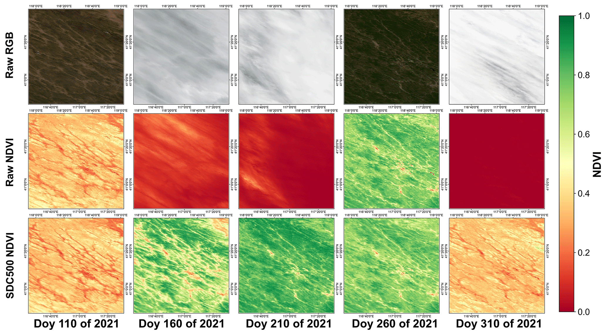
Figure 13Assessment of spatial pattern in a cropland area (site S5). True-colour composite (red: band 1, green: band 4, and blue: band 3) and raw MODIS NDVI and SDC500 NDVI imageries on 5 dates in 2021.
Figure 14 presents a demonstration of the raw and reconstructed reflectance and NDVI time series in S6, which is in a mid-latitude evergreen broadleaf forest area. Like the other sites, the SDC500 dataset in S6 successfully restored the image series of evergreen broadleaf forest: the annual variation of NDVI is within the range 0.3–0.5; the influence of outliers, such as on DOY 100, 252, and 272 in Fig. 14a, has been satisfactorily eliminated.
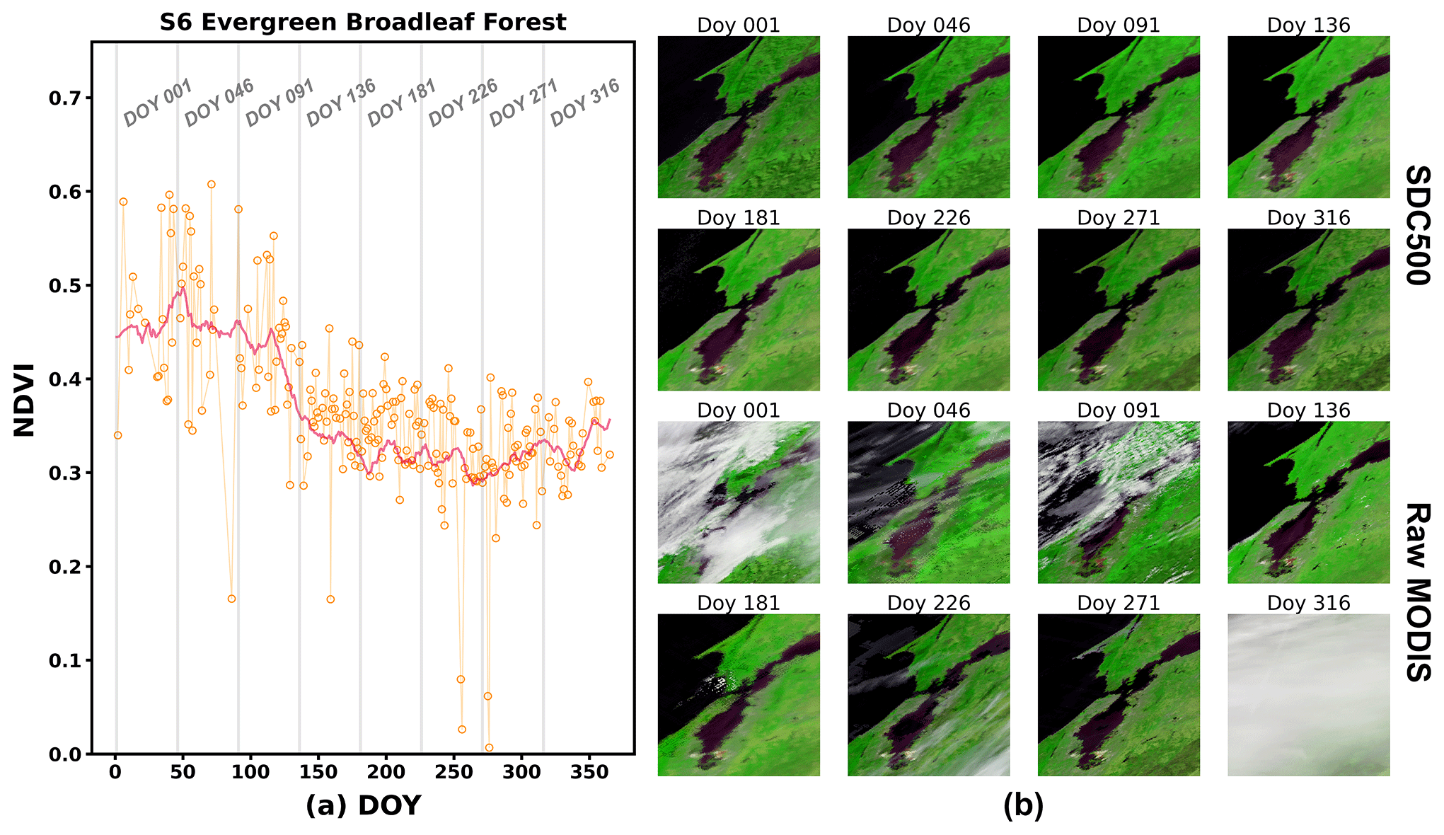
Figure 14Performance of SDC in site S6. (a) The NDVI curves for the central pixel; the orange points indicate the valid MODIS observations, and the red line indicates the SDC500 results. (b) The spatial pattern of image blocks of 200×200 pixels centred around the site (red: band 1, green: band 2, and blue: band 3).
4.5 SDC500 in snow-dominant areas
The SDC500 demonstrates excellent capability in dealing with snow and ice cover. Figure 15 illustrates its accurate representation of the melting and snowfall processes while retaining the intricate features of needleleaf forests hidden beneath snow and ice. Even in images where both snow and vegetation are present, the SDC maintains spatial continuity effectively. In the Arctic region depicted in Fig. 16, the SDC500 successfully captures the short melting process in summer (DOY 180–270), showing its ability to document the variations in snow and ice cover over time.
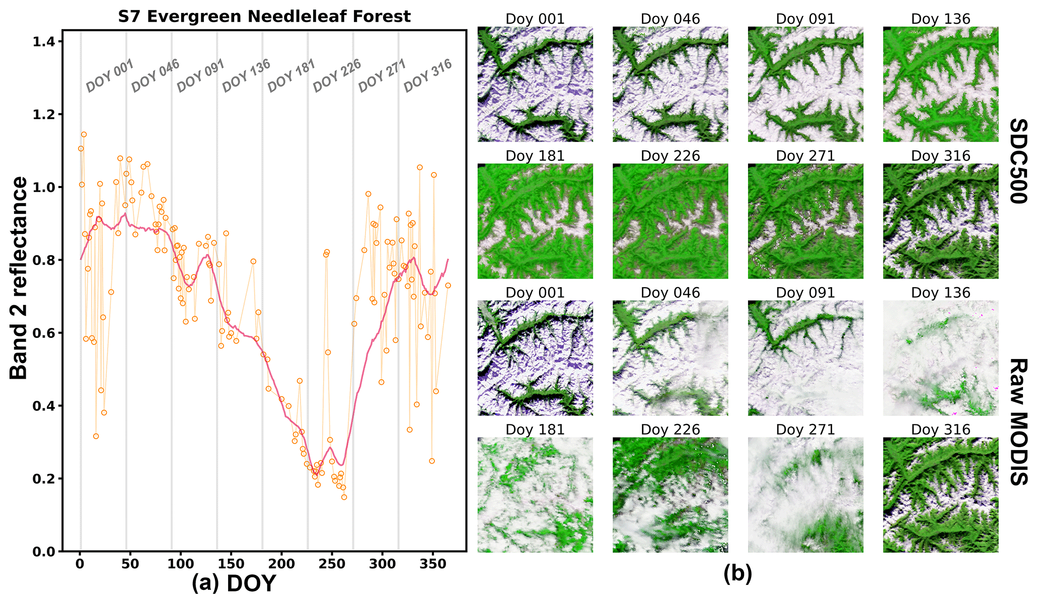
Figure 15Performance of SDC in site S7. (a) The band-2 reflectance curves for the central pixel; the orange points indicate the valid MODIS observation, and the red line indicates the SDC500 results. (b) The spatial pattern of image blocks of 200×200 pixels centred around the site (red: band 1, green: band 2, and blue: band 3).
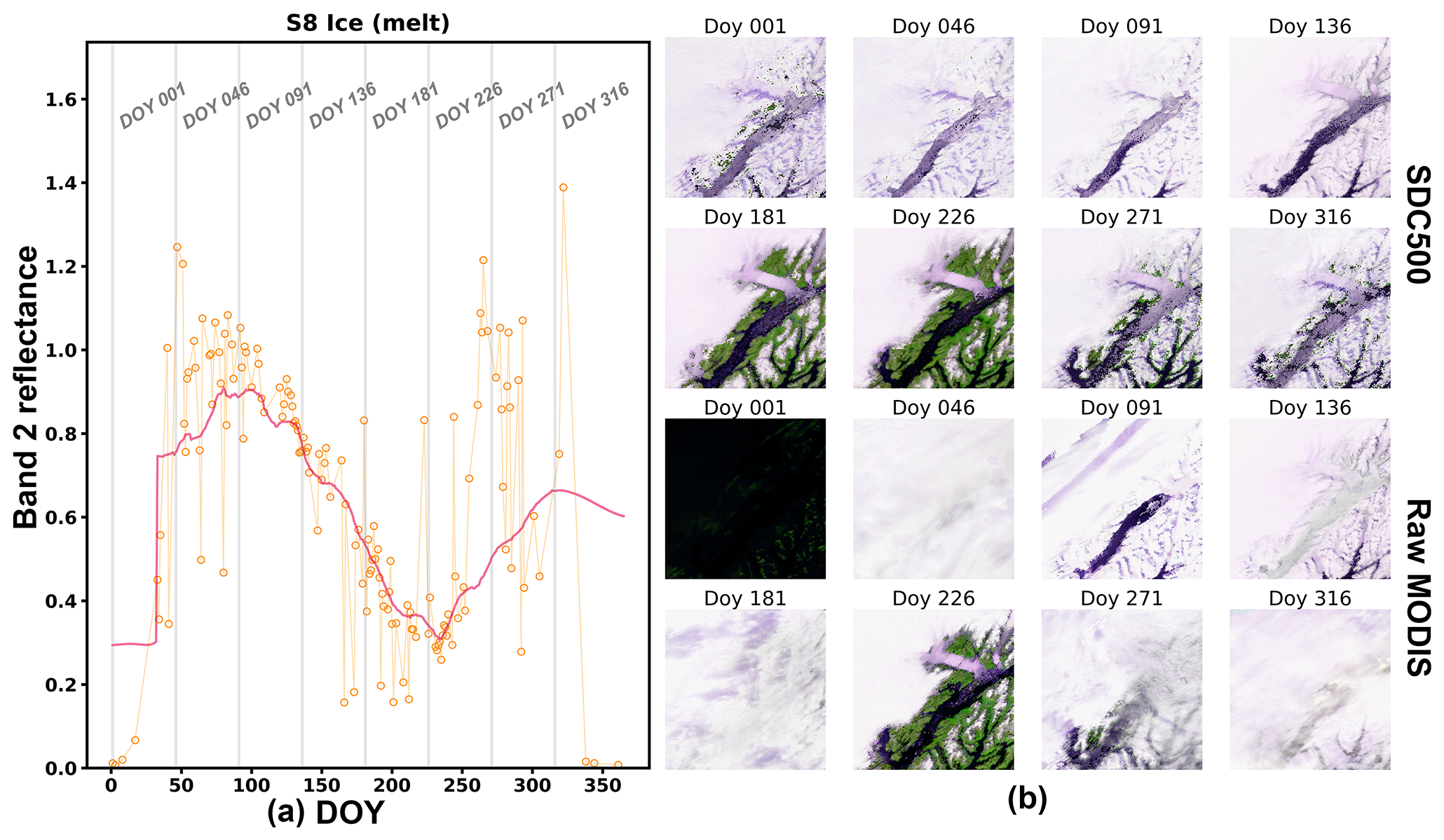
Figure 16Performance of SDC in site S8. (a) The band-2 reflectance curves for the central pixel; the orange points indicate the valid MODIS observation, and the red line indicates the SDC500 results. (b) The spatial pattern of image blocks of 200×200 pixels centred around the site (red: band 1, green: band 2, and blue: band 3).
5.1 Quantitative assessment of the BRDF correction method
In this study, we perform BRDF correction using land cover information from the MCD12Q1 dataset and kernel model parameters from the MCD43A1 dataset. Thus, the uncertainty in these two datasets may result in uncertainty in the BRDF-corrected result. As there is no established ground-truth dataset for land surface BRDF at the 500 m resolution, we evaluate the uncertainty of our proposed BRDF correction method through two approaches: (1) a visual comparison of the MODIS observations before and after the BRDF correction and (2) a quantitative comparison with the MODIS nadir BRDF-adjusted reflectance dataset MCD43A4.
Figure 17 presents a comparison of the time series of raw MODIS observations and BRDF correction results in four typical sites. In Fig. 17, the raw clear observations are directly extracted from the MOD09GA dataset, corresponding to the various sun/view geometries of the actual satellite overpass; the BRDF-corrected results are standardized to the nadir view angle and sun angle of 10:30 local time. As shown in Fig. 17, the BRDF-corrected results become more consistent with each other after normalization, with reduced noise from biased marginal values and, to some extent, alleviated abnormal fluctuations. We also noticed that there are still remanent fluctuations in the normalized reflectance series; this is partly due to the reduced spatial resolution of BRDF parameters in the a priori database and partly due to other sources of uncertainties such as geometric alignment error and atmosphere correction error.
In addition, we conducted quantitative validation between the proposed BRDF-corrected results and the MODIS nadir BRDF-adjusted reflectance dataset MCD43A4 in the four tiles (h11v09, h20v10, h27v05, and h16v02) corresponding to the typical sites S9, S10, S11, and S12. For each MODIS tile, a regular grid of 12×12 pixels was selected as sample pixels. The raw MODIS observations in 2010, along with their corresponding normalized values, were validated against the MODIS NBAR product MCD43A4. The results, shown in Fig. 18, demonstrate that the raw MODIS reflectance shows a remarkable difference compared to the MCD43A4 product, with an RMSE of 0.275 and a bias of 0.1721; in comparison, our BRDF correction method is in good agreement with the MCD43A4 product, with an RMSE of 0.056 and a bias of −0.0085. As SDC500 and MCD43A4 are derived using different methods but are consistent with each other, the consistency indicates that they both provide accurate results.
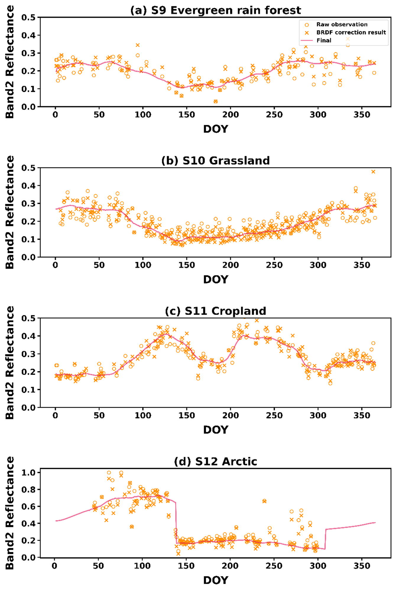
Figure 17Example of series of raw MODIS observations, BRDF-corrected observations, and the final smoothed series in four typical sites: site S9 evergreen rain forest (a), site S10 grassland (b), site S11 cropland (c), and site S12 arctic (d).
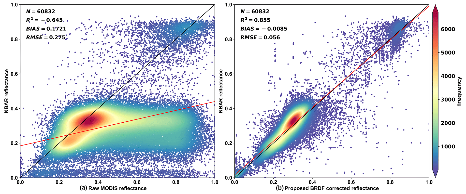
Figure 18Quantitative evaluation of our proposed BRDF correction method: (a) raw MODIS reflectance vs. MODIS NBAR product and (b) SDC500 dataset vs. MODIS NBAR product.
5.2 Quantitative assessment of the gap-filling method
An essential module in the data-processing algorithm is outlier detection and gap filling. In extreme situations of long-lasting cloud coverage, which commonly happens in tropical and monsoon areas, the gap-filling strategy basically determines the shape of the final output time series. In the past, it is common practice in time series reconstruction that the invalid values should be masked out and filled with linear interpolation of valid values before applying the smoothing filter (e.g. the SG filter) to the time series. In this study, we use a combination of phenology-based and spline-based fitting to fill the gaps. Besides, during the time series fitting, outlier values are detected and masked. As the outlier values are most likely incorrectly flagged cloud or cloud shadow pixels, the exclusion of them can further promote the stability of the reconstruction result.
To demonstrate the performance of our proposed gap-filling algorithm in comparison to the linear gap filling, we select an extreme case in the monsoon season in southern Asia. Figure 19a shows an area of 600×1000 pixels in MODIS tile h25v07, which is located in central India. The monsoon brings heavy cloud and precipitation in June and July every year and leaves almost no clear observations for optical remote sensing satellites in these two continuous months. Figure 19b presents the average cloud coverage of this area for each Julian day from 2000 to 2022, as well as the cloud coverage in the year 2019. We can see that there is a rare case of a clear window during Julian days 196 to 198 in 2019, which can serve as a reference truth value to validate the output of the time series reconstruction algorithm. From Fig. 19a it is found that the clear area is only in the centre part of the image; the surroundings are still contaminated with clouds. Thus, we manually outlined the clear area as a region of interest (ROI) to derive validation statistics.
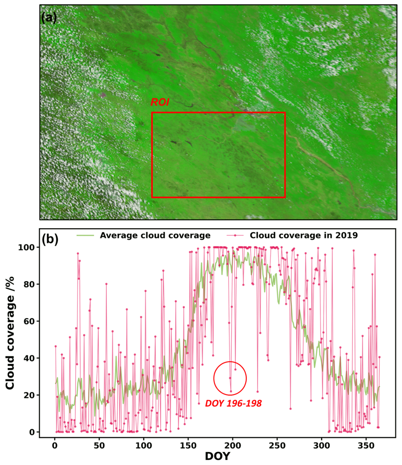
Figure 19Study area of quantitative validation. (a) Original MODIS observation on 2019 DOY 197 in tile h25v07, line 1–600, column 801–1800. Red: band 1, green: band 2, and b: band 3. The region of interest (ROI) outlined by the red box indicates the clear area to derive validation statistics. (b) Average cloud coverage in the period of 2000–2022 and cloud coverage in 2019.
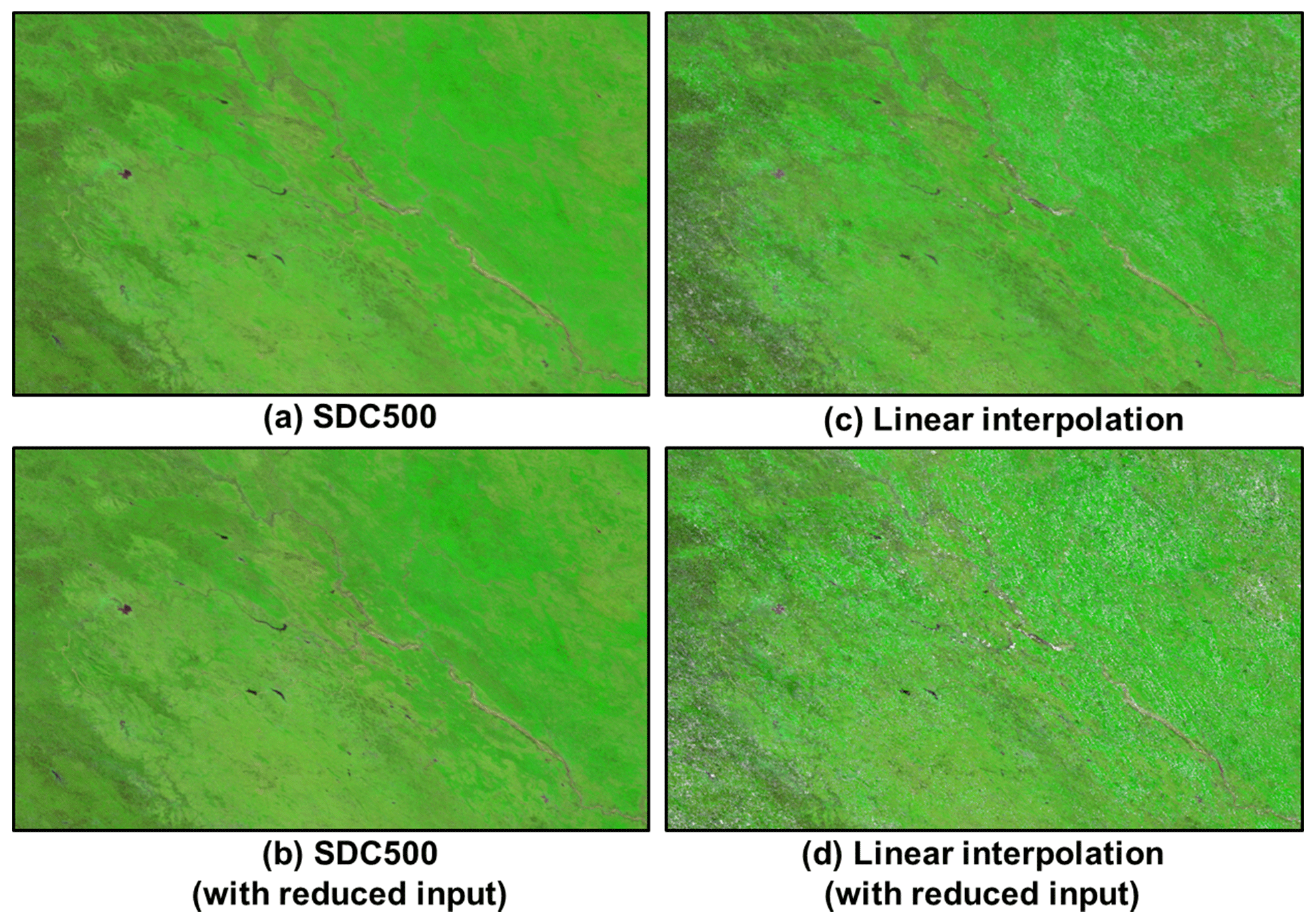
Figure 20Reconstructed results on 2019 DOY 197 in four cases: (a) SDC500 with all valid input data (case 1), (b) linear interpolation with all valid input data (case 2), (c) SDC500 with reduced input data (case 3), and (d) linear interpolation with reduced input data (case 4).
Table 2Quantitative validation of linear interpolation and SDC500 in different bands.
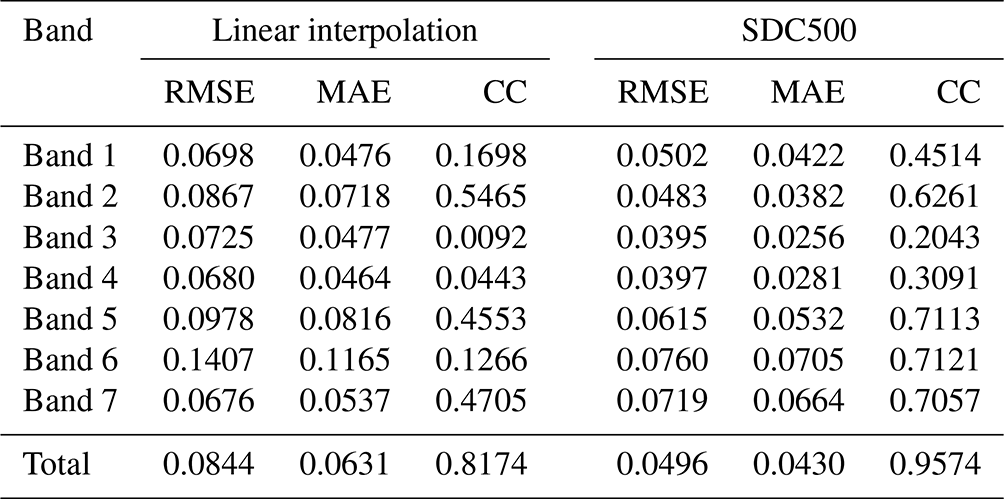
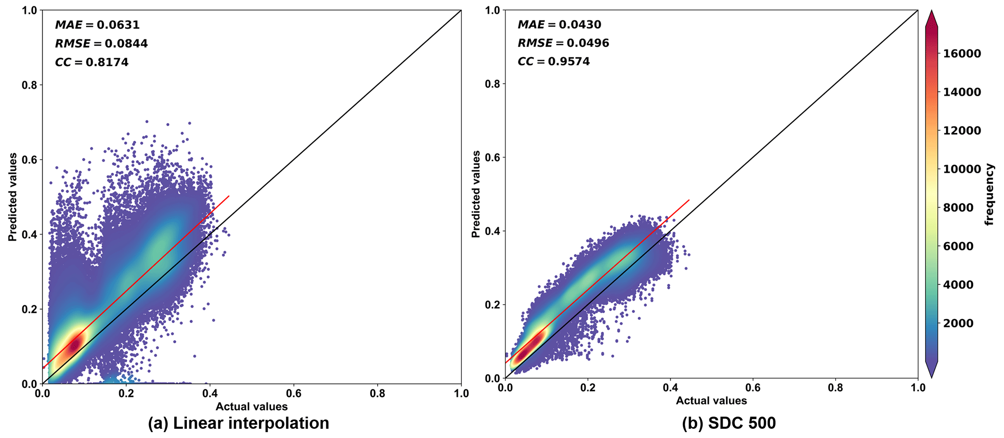
Figure 21Quantitative comparison between actual values and predicted values of linear interpolation (a) and SDC500 (b).
We implemented the algorithm in four cases to reconstruct the image series in 2019. Case 1 represents the operational run of the SDC500 gap-filling and smoothing algorithm, with all the available MODIS observations as input. Case 2 is the same algorithm with an imaginary scenario of reduced input in which MODIS observations in Julian days 195 to 199 are excluded from the input dataset; the purpose of this scenario is to simulate a long gap which occurs in other years. Case 3 is a comparison case in which linear gap filling and SG filter smoothing are applied to the same input data as in case 1. Case 4 is a comparison case in which linear gap filling and SG filter smoothing are applied to the reduced input data, as in case 2. Figure 20 illustrates the reconstructed images of the four cases; the good results of Fig. 20a and b indicate that the SDC500's gap-filling results exhibit improved spatial continuity and greater robustness with reduced input. In terms of performance evaluation metrics, lower values of root-mean-square error (RMSE) and mean absolute error (MAE), as well as a higher correlation coefficient (CC), indicate better results. Table 2 and Fig. 21 provide the quantitative comparison between SDC500 and the result of linear interpolation. The SDC500 achieves am RMSE of 0.0496, a MAE of 0.0430, and a CC of 0.9574, demonstrating superior accuracy compared to the result of linear interpolation, which yields an RMSE of 0.0844, a MAE of 0.0631, and a CC of 0.8174.
5.3 Performance of SDC500 in capturing rapid disturbance
The SDC500 product provides high-resolution observations with accurate characterization of the long-term phenology of ecosystems while also retaining the useful localized feature of rapid disturbances. In this study, we chose to demonstrate the product's capability to detect such disturbances in two wildfire events. The first event is the largest recorded tundra fire that occurred near Anaktuvuk River (Jones et al., 2009), which was started by a lightning strike in July 2007 and spread across a large area of 1039 km2 till September. The other event is a serious forest fire that occurred in Australia in July 2019, which was caused by drought and heat weave weather and raged for months. To enhance the extent of the burned area, we computed the normalized burnt ratio (NBR) index, with a lower NBR indicating a higher fraction of burned area. Spatially, the SDC500 was able to capture the continuous spreading pattern of the wildfires, as demonstrated in Figs. 22 and 23. Temporally, the NBR decreased sharply during the fires and returned to normal values after the Australia forest wildfire, as seen in Fig. 23b, while remaining low after the Arctic tundra wildfire, as shown in Fig. 22b. However, as the algorithm of SDC500 is based on temporal smoothing, the reconstructed time series of NBR demonstrate a gradual change, though there should be an abrupt change of NBR in the fire events. Data users need to be aware of the uncertainty caused by this smooth-out effect.
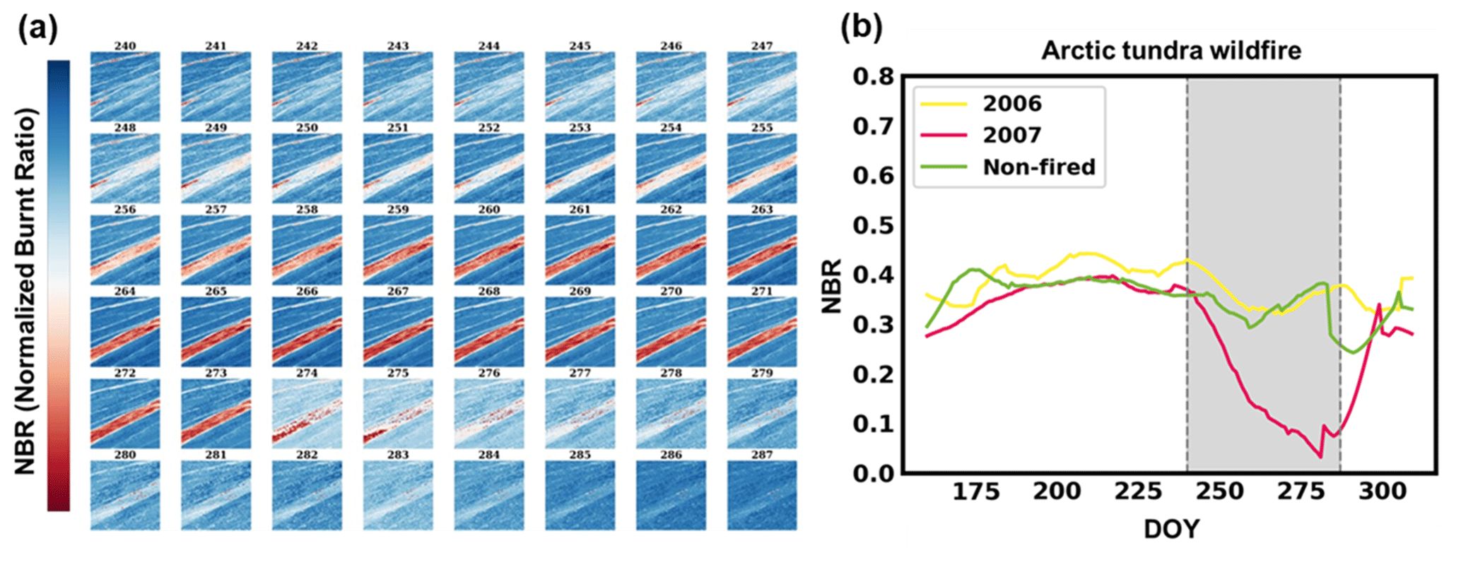
Figure 22The performance of SDC500 during the Arctic tundra wildfire in 2007 summer. (a) The spatial pattern of NBR. (b) The NBR series for a central pixel of burned area in 2006 (before burn) and 2007 (burn) and a non-fired pixel in 2007.
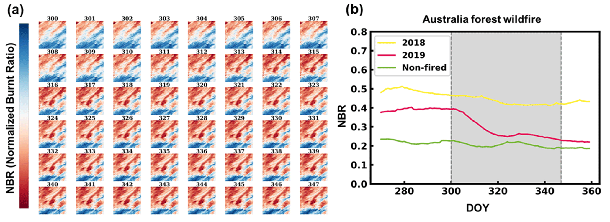
Figure 23The performance of SDC500 during the Australia forest wildfire. (a) The spatial pattern of NBR. (b) A central pixel of burned area in 2018 (before burn) and 2019 (burn) and a non-fired pixel in 2019.
5.4 Quality assessment (QA) and limitations of SDC500
This study proposes an advanced framework for reconstructing the spatiotemporally seamless MODIS surface reflectance dataset. The preliminary evaluations demonstrate the effectiveness of the SDC500 in addressing the challenge of missing key points, filling isolated and continuous gaps, as well as gaps at peaks and valleys. Moreover, the SDC500 successfully reduces noise from biased outlier values and eliminates abnormal fluctuations caused by observation conditions rather than true land surface dynamics.
Despite the satisfactory results achieved using the proposed methodology, uncertainties should be assessed as auxiliary information to support various applications of data users. Pixelwise quality assessment (QA) is the commonly adopted means to express the uncertainties in the dataset, which is also adopted here. Although the ideal way is to express the uncertainties quantitatively, it is not applicable in the current version of SDC500 for two reasons: (1) the data-processing chain contains many sub-algorithms, as well as feedbacks, which make the quantitative uncertainty assessment very difficult, and (2) there is still a lack of quantitative uncertainty indication for the input data of surface reflectance. Thus, the QA flag of SDC500 only gives a relative indicator to the quality of the reconstructed reflectance value. In the QA flag, which is 16 bits unsigned integer, the overall quality is indicated in the lowest 2 bits, i.e. bits 0–1, with 00 representing the best credibility and 11 representing the worst credibility. Figure 24 presents the average percentage for the overall quality bits in each MODIS tile over the year 2020. Pixels over ocean and pixels in polar night are excluded from the percentage statistics. It shows that the tiles with low-quality pixels are mainly distributed in the tropical and subtropical zones or in tiles over small islands, while the main reason for the decreased quality is heavy cloud coverage.
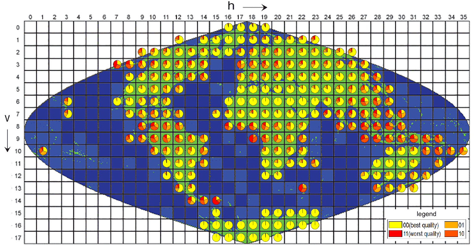
Figure 24The average percentage for the overall quality bits of QA flag in each MODIS tile over the year 2020.
Apart from the QA flag, some of the known issues have not been addressed in the current version of algorithm and may bring extra uncertainties to the final product. Firstly, topographic effect is very important and may bring large uncertainty in the remote sensing estimated surface parameters (Wen et al., 2018). However, the operational topology correction method is mostly empirical rather than quantitative, and topographic research in the resolution of 500 m is even more scarce. Thus, topology is totally ignored in our current version of the algorithm, and data users should take extra caution when using the SDC500 product in mountainous areas. Secondly, the mixed-pixel issue is also not addressed in our current version of the algorithm. Mixed pixels widely exist in 500 m resolution MODIS data. If the pixel is composed of the same or similar land covers, the influence is small. But if the pixel is located in a distinct boundary, such as between land and water or between rural and urban areas, the uncertainty of the reconstructed reflectance will increase, but this is not indicated in the QA flag.
Some other issues have only been partly addressed and need to be improved upon in future research. For example, the BRDF correction relies heavily on a priori parameters derived from the MCD43A1 dataset and the empirical RTLSR model. However, the RTLSR model, which was originally designed for vegetated land pixels, may not perform well in snow- or ice-covered surfaces and water bodies, leading to higher uncertainty in the SDC500 for these areas compared to vegetated and arid regions. The current granularity used to derive the statistics of BRDF parameters is 100 km × 100 km, which may be too coarse and result in some loss of accuracy. Our future research should focus on exploring enhancements to the BRDF model and parameterization. In terms of prolonged gaps caused by cloudy days, there are still extreme cases that cannot be adequately filled using the proposed algorithm. Visual inspection has identified that these extreme cases occur mostly in mountainous terrain within tropical rainforest climate zones. In these areas, the topographic cloud formed by the terrain effect persists throughout the year, resulting in almost no clear satellite images. Another noteworthy case is the transition between snow-covered and snow-free states in high-latitude areas. As described in Sect. 3.5, the observations in a pixel's time series are divided into two groups, snow covered and snow free, and are processed separately. When these two results are combined, the final series may exhibit discontinuities around the switching date. Furthermore, the current algorithm struggles to robustly reconstruct images near the date of surface status change, presenting a challenging research topic.
In general, the process of image reconstruction involves altering the original values of sensor observations and replacing them with approximated values. Therefore, the reconstructed dataset is primarily intended to support large-scale statistical research or discrete applications such as land cover classification rather than small-scale or in-depth research such as model tuning and validation. In the past, people have tended to be overcautious when sharing the reconstructed dataset, being fearful of misleading data users. However, the demand for seamless data cubes has prompted us to share the SDC500 dataset and to provide an opportunity for evaluation and improvement by the wider public.
The SDC500 is available at http://data.starcloud.pcl.ac.cn/resource/27 (Liang et al., 2023b) or https://doi.org/10.12436/SDC500.27.20230701 (Liang et al., 2023a). All users are welcome to freely download it. This dataset covers all global land surface, as well as part of shallow-sea areas, in the temporal range of 2000–2022. The spatial resolution is 500 m, and the temporal resolution is 1 d. The dataset is stored in GEOTIFF format and Sinusoidal projection. The dataset is composed of eight bands. The first seven bands correspond to surface reflectance in the MODIS band 1 to band 7, with a scale value of 0.0001 to convert digital number (DN) values to reflectance. The eighth band is the quality assessment (QA) flag, in which the overall quality is indicated in the lowest two bits, i.e. bits 0–1, with 00 representing the best credibility and 11 representing the worst credibility, and bit 6 being an indicator of snow status, with value 0 indicating snow free and value 1 indicating snow; bit 7 is an indicator of polar night, with value 0 meaning normal and value 1 indicating that the pixel is in polar night (solar zenith angle larger than 82 ∘ at 10:30 local time) in the specified date.
The GEE code used to derive BRDF parameters from MCD43A1 and MCD12Q1 products can be accessed at https://code.earthengine.google.com/363b4d94090048f9e28103ad3efebfdf (Liu, 2022).
The state-of-art Moderate Resolution Imaging Spectroradiometer (MODIS) surface reflectance products suffer from temporal and spatial gaps, which make it difficult to characterize the continuous variation of the terrestrial surface. There are two challenges in reconstructing spatiotemporal seamless surface reflectance: first, the intrinsic inconsistency of observations owing to various sun/view geometries, and second, the prolonged missing values resulting from heavy cloud coverage, especially in monsoon season or polar night.
In this study, we have established a framework to address these two challenges. The first global 500 m daily seamless data cubes (SDC500) of surface reflectance were produced based on MODIS products, covering the period from 2000 to 2022. The proposed framework contains the generation of a land-cover-based a priori database, BRDF correction, outlier detection, gap filling, and smoothing. In consideration of the fact that the change in surface reflectance is abrupt in the snow–thaw process, the time sequence is divided into the snow-covered and snow-free parts and processed separately.
The quantitative assessment showed that proposed gap-filling results have an RMSE of 0.0496 and a MAE of 0.0430. In addition, the proposed BRDF correction results showed an RMSE of 0.056 and a bias of −0.0085 when compared with MODIS NBAR products, indicating the acceptable accuracy of both products. Furthermore, assessment of SDC500 at 12 sites worldwide with different land covers demonstrated its robust performance in tropical and subtropical areas (sites S1, S2), acrid areas (sites S3, S4), temperate climate areas (sites S5, S6), and snow-dominant areas (sites S7, S8). From a temporal perspective, the SDC500 eliminates abnormal fluctuations while retaining the useful localized feature of rapid disturbances. From a spatial perspective, the SDC500 shows satisfactory spatial continuity.
The SDC500 product can serve as fundamental input for ecological, agricultural, and environmental applications and quantitative remote sensing studies, eliminating the time-consuming and labour-intensive preprocesses that is typically required. In addition, the SDC500 dataset will be a necessary step towards the generation of a new version of 30 m resolution seamless data cubes (Liu et al., 2021), which will greatly improve the global land use and land cover classification accuracy, as well as capture its dynamics.
QL conceptualized and supervised the project. QL, XL, and JW designed the workflow of the methodology to produce the dataset. QL, XL, JW, and SC conducted the work in data acquisition and processing. QL and XL performed data analysis and prepared the paper. JW, SC, and PG reviewed and edited the draft. All the authors contributed to the interpretation of the results.
The contact author has declared that none of the authors has any competing interests.
Publisher's note: Copernicus Publications remains neutral with regard to jurisdictional claims made in the text, published maps, institutional affiliations, or any other geographical representation in this paper. While Copernicus Publications makes every effort to include appropriate place names, the final responsibility lies with the authors.
This research was partially supported by two NSFC grants (nos. 42090015 and 42071400) and the Major Key Project of PCL. We would like to thank NASA for providing the MODIS data products.
This research has been supported by the National Natural Science Foundation of China (grant nos. 42071400 and 42090015).
This paper was edited by Dalei Hao and reviewed by Ricardo Dal Agnol da Silva and two anonymous referees.
Barnes, W. L., Pagano, T. S., and Salomonson, V. V.: Prelaunch characteristics of the moderate resolution imaging spectroradiometer (MODIS) on EOS-AM1, IEEE T. Geosci. Remote, 36, 1088–1100, https://doi.org/10.1109/36.700993, 1998.
Cao, R., Chen, Y., Shen, M., Chen, J., Zhou, J., Wang, C., and Yang, W.: A simple method to improve the quality of NDVI time-series data by integrating spatiotemporal information with the Savitzky-Golay filter, Remote Sens. Environ., 217, 244–257, https://doi.org/10.1016/j.rse.2018.08.022, 2018.
Cao, S., Li, M., Zhu, Z., Wang, Z., Zha, J., Zhao, W., Duanmu, Z., Chen, J., Zheng, Y., Chen, Y., Myneni, R. B., and Piao, S.: Spatiotemporally consistent global dataset of the GIMMS leaf area index (GIMMS LAI4g) from 1982 to 2020, Earth Syst. Sci. Data, 15, 4877–4899, https://doi.org/10.5194/essd-15-4877-2023, 2023.
Chen, C., Park, T., Wang, X., Piao, S., Xu, B., Chaturvedi, R. K., Fuchs, R., Brovkin, V., Ciais, P., Fensholt, R., Tømmervik, H., Bala, G., Zhu, Z., Nemani, R. R., and Myneni, R. B.: China and India lead in greening of the world through land-use management, Nat. Sustain., 2, 122–129, https://doi.org/10.1038/s41893-019-0220-7, 2019.
Chen, J., Jönsson, P., Tamura, M., Gu, Z., Matsushita, B., and Eklundh, L.: A simple method for reconstructing a high-quality NDVI time-series data set based on the Savitzky–Golay filter, Remote Sens. Environ., 91, 332–344, https://doi.org/10.1016/j.rse.2004.03.014, 2004.
Chen, M., Willgoose, G. R., and Saco, P. M.: Investigating the impact of leaf area index temporal variability on soil moisture predictions using remote sensing vegetation data, J. Hydrol., 522, 274–284, https://doi.org/10.1016/j.jhydrol.2014.12.027, 2015.
Chen, Y., Cao, R., Chen, J., Liu, L., and Matsushita, B.: A practical approach to reconstruct high-quality Landsat NDVI time-series data by gap filling and the Savitzky–Golay filter, ISPRS J. Photogramm., 180, 174–190, https://doi.org/10.1016/j.isprsjprs.2021.08.015, 2021.
Chu, D., Shen, H., Guan, X., Chen, J. M., Li, X., Li, J., and Zhang, L.: Long time-series NDVI reconstruction in cloud-prone regions via spatio-temporal tensor completion, Remote Sens. Environ., 264, 112632, https://doi.org/10.1016/j.rse.2021.112632, 2021.
Claverie, M., Vermote, E. F., Franch, B., and Masek, J. G.: Evaluation of the Landsat-5 TM and Landsat-7 ETM+ surface reflectance products, Remote Sens. Environ., 169, 390–403, https://doi.org/10.1016/j.rse.2015.08.030, 2015.
Estoque, R. C.: A review of the sustainability concept and the state of SDG monitoring using remote sensing, Remote Sens., 12, 1770, https://doi.org/10.3390/rs12111770, 2020.
Fang, H., Baret, F., Plummer, S., and Schaepman-Strub, G.: An Overview of Global Leaf Area Index (LAI): Methods, Products, Validation, and Applications, Rev. Geophys., 57, 739–799, https://doi.org/10.1029/2018RG000608, 2019.
Fang, H., Liang, S., Townshend, J. R., and Dickinson, R. E.: Spatially and temporally continuous LAI data sets based on an integrated filtering method: Examples from North America, Remote Sens. Environ., 112, 75–93, https://doi.org/10.1016/j.rse.2006.07.026, 2008.
Fensholt, R. and Proud, S. R.: Evaluation of Earth Observation based global long term vegetation trends – Comparing GIMMS and MODIS global NDVI time series, Remote Sens. Environ., 119, 131–147, https://doi.org/10.1016/j.rse.2011.12.015, 2012.
Friedl, M. A., McIver, D. K., Hodges, J. C. F., Zhang, X. Y., Muchoney, D., Strahler, A. H., Woodcock, C. E., Gopal, S., Schneider, A., Cooper, A., Baccini, A., Gao, F., and Schaaf, C.: Global land cover mapping from MODIS: algorithms and early results, Remote Sens. Environ., 83, 287–302, https://doi.org/10.1016/S0034-4257(02)00078-0, 2002.
Gray, J., Sulla-Menashe, D., and Friedl, M. A.: User guide to collection 6 modis land cover dynamics (mcd12q2) product, NASA EOSDIS Land Processes DAAC: Missoula, MT, USA, 6, 1–8, 2019.
Jia, A., Liang, S., Wang, D., Ma, L., Wang, Z., and Xu, S.: Global hourly, 5 km, all-sky land surface temperature data from 2011 to 2021 based on integrating geostationary and polar-orbiting satellite data, Earth Syst. Sci. Data, 15, 869–895, https://doi.org/10.5194/essd-15-869-2023, 2023.
Jiang, C., Ryu, Y., Fang, H., Myneni, R., Claverie, M., and Zhu, Z.: Inconsistencies of interannual variability and trends in long-term satellite leaf area index products, Glob. Change Biol., 23, 4133–4146, https://doi.org/10.1111/gcb.13787, 2017.
Jiang, Y., Wang, J., and Wang, Y.: Daily Evapotranspiration Estimations by Direct Calculation and Temporal Upscaling Based on Field and MODIS Data, Remote Sens., 14, 4094, https://doi.org/10.3390/rs14164094, 2022.
Jones, B. M., Kolden, C. A., Jandt, R., Abatzoglou, J. T., Urban, F., and Arp, C. D.: Fire behavior, weather, and burn severity of the 2007 anaktuvuk river tundra fire, North Slope, Alaska, Arct. Antarct. Alp. Res., 41, 309–316, https://doi.org/10.1657/1938-4246-41.3.309, 2009.
Ju, J., Roy, D. P., Shuai, Y., and Schaaf, C.: Development of an approach for generation of temporally complete daily nadir MODIS reflectance time series, Remote Sens. Environ., 114, 1–20, https://doi.org/10.1016/j.rse.2009.05.022, 2010.
Ju, J., Roy, D. P., Vermote, E., Masek, J., and Kovalskyy, V.: Continental-scale validation of MODIS-based and LEDAPS Landsat ETM+ atmospheric correction methods, Remote Sens. Environ., 122, 175–184, https://doi.org/10.1016/j.rse.2011.12.025, 2012.
Justice, C., Townshend, J., Vermote, E., Masuoka, E., Wolfe, R., Saleous, N., Roy, D., and Morisette, J.: An overview of MODIS Land data processing and product status, Remote Sens. Environ., 83, 3–15, https://doi.org/10.1016/S0034-4257(02)00084-6, 2002.
Kawala-Sterniuk, A., Podpora, M., Pelc, M., Blaszczyszyn, M., Gorzelanczyk, E. J., Martinek, R., and Ozana, S.: Comparison of Smoothing Filters in Analysis of EEG Data for the Medical Diagnostics Purposes, Sensors, 20, 807, https://doi.org/10.3390/s20030807, 2020.
Li, M., Cao, S., Zhu, Z., Wang, Z., Myneni, R. B., and Piao, S.: Spatiotemporally consistent global dataset of the GIMMS Normalized Difference Vegetation Index (PKU GIMMS NDVI) from 1982 to 2022, Earth Syst. Sci. Data, 15, 4181–4203, https://doi.org/10.5194/essd-15-4181-2023, 2023.
Liang, X., Mao, W., Yang, K., and Ji, L.: Automated Small River Mapping (ASRM) for the Qinghai-Tibet Plateau Based on Sentinel-2 Satellite Imagery and MERIT DEM, Remote Sens., 14, 4693, https://doi.org/10.3390/rs14194693, 2022.
Liang, X., Liu, Q., Wang, J., Chen, S., and Gong, P.: Global 500 m seamless dataset (2000–2022) of land surface reflectance generated from MODIS products, Peng cheng laboratory [data set], https://doi.org/10.12436/SDC500.27.20230701, 2023a.
Liang, X., Liu, Q., Wang, J., Chen, S., and Gong, P.: Global 500 m seamless dataset (2000–2022) of land surface reflectance generated from MODIS products, http://data.starcloud.pcl.ac.cn/resource/27, last access: 25 December 2023b.
Liu, H., Gong, P., Wang, J., Wang, X., Ning, G., and Xu, B.: Production of global daily seamless data cubes and quantification of global land cover change from 1985 to 2020-iMap World 1.0, Remote Sens. Environ., 258, 112364, https://doi.org/10.1016/j.rse.2021.112364, 2021.
Liu, N. F., Liu, Q., Wang, L. Z., Liang, S. L., Wen, J. G., Qu, Y., and Liu, S. H.: A statistics-based temporal filter algorithm to map spatiotemporally continuous shortwave albedo from MODIS data, Hydrol. Earth Syst. Sci., 17, 2121–2129, https://doi.org/10.5194/hess-17-2121-2013, 2013.
Liu, Q.: BRDF parameters generation, https://code.earthengine.google.com/363b4d94090048f9e28103ad3efebfdf, last access: 25 October 2022.
Liu, R., Shang, R., Liu, Y., and Lu, X.: Global evaluation of gap-filling approaches for seasonal NDVI with considering vegetation growth trajectory, protection of key point, noise resistance and curve stability, Remote Sens. Environ., 189, 164–179, https://doi.org/10.1016/j.rse.2016.11.023, 2017.
Liu, Y., Liu, R., and Chen, J. M.: Retrospective retrieval of long-term consistent global leaf area index (1981–2011) from combined AVHRR and MODIS data, J. Geophys. Res.-Biogeo., 117, G04003, https://doi.org/10.1029/2012JG002084, 2012.
Lizundia-Loiola, J., Otón, G., Ramo, R., and Chuvieco, E.: A spatio-temporal active-fire clustering approach for global burned area mapping at 250 m from MODIS data, Remote Sens. Environ., 236, 111493, https://doi.org/10.1016/j.rse.2019.111493, 2020.
Ma, H. and Liang, S.: Development of the GLASS 250-m leaf area index product (version 6) from MODIS data using the bidirectional LSTM deep learning model, Remote Sens. Environ., 273, 112985, https://doi.org/10.1016/j.rse.2022.112985, 2022.
Ma, H., Liang, S., Xiong, C., Wang, Q., Jia, A., and Li, B.: Global land surface 250 m 8 d fraction of absorbed photosynthetically active radiation (FAPAR) product from 2000 to 2021, Earth Syst. Sci. Data, 14, 5333–5347, https://doi.org/10.5194/essd-14-5333-2022, 2022.
Mao, D., Wang, Z., Luo, L., and Ren, C.: Integrating AVHRR and MODIS data to monitor NDVI changes and their relationships with climatic parameters in Northeast China, Int. J. Appl. Earth Obs., 18, 528–536, https://doi.org/10.1016/j.jag.2011.10.007, 2012.
Moody, E. G., King, M. D., Platnick, S., Schaaf, C. B., and Gao, F.: Spatially complete global spectral surface albedos: value-added datasets derived from Terra MODIS land products, IEEE T. Geosci. Remote, 43, 144–158, https://doi.org/10.1109/TGRS.2004.838359, 2005.
Schaaf, C., Wang, Z., Shuai, Y., and Strahler, A.: Daily operational MODIS BRDF, albedo and nadir reflectance products (V006), AGU Fall Meeting Abstracts, B34D-07, 2012.
Schaaf, C. B., Gao, F., Strahler, A. H., Lucht, W., Li, X., Tsang, T., Strugnell, N. C., Zhang, X., Jin, Y., Muller, J.-P., Lewis, P., Barnsley, M., Hobson, P., Disney, M., Roberts, G., Dunderdale, M., Doll, C., d'Entremont, R. P., Hu, B., Liang, S., Privette, J. L., and Roy, D.: First operational BRDF, albedo nadir reflectance products from MODIS, Remote Sens. Environ., 83, 135–148, https://doi.org/10.1016/S0034-4257(02)00091-3, 2002.
Sulla-Menashe, D. and Friedl, M. A.: User guide to collection 6 MODIS land cover (MCD12Q1 and MCD12C1) product, USGS, Reston, Va, Usa, 1, 18, 2018.
Sun, Q., Wang, Z., Li, Z., Erb, A., and Schaaf, C. B.: Evaluation of the global MODIS 30 arc-second spatially and temporally complete snow-free land surface albedo and reflectance anisotropy dataset, Int. J. Appl. Earth Obs., 58, 36–49, https://doi.org/10.1016/j.jag.2017.01.011, 2017.
Tang, H., Yu, K., Hagolle, O., Jiang, K., Geng, X., and Zhao, Y.: A cloud detection method based on a time series of MODIS surface reflectance images, Int. J. Digit. Earth, 6, 157–171, https://doi.org/10.1080/17538947.2013.833313, 2013.
Vermote, E., Kotchenova, S., and Ray, J.: MODIS Surface Reflectance user's guide, version 1.3, MODIS Land Surface Reflectance Science Computing Facility, 2011.
Vermote, E., Justice, C., Claverie, M., and Franch, B.: Preliminary analysis of the performance of the Landsat 8/OLI land surface reflectance product, Remote Sens. Environ., 185, 46–56, https://doi.org/10.1016/j.rse.2016.04.008, 2016.
Vermote, E. F., El Saleous, N., Justice, C. O., Kaufman, Y. J., Privette, J. L., Remer, L., Roger, J. C., and Tanré, D.: Atmospheric correction of visible to middle-infrared EOS-MODIS data over land surfaces: Background, operational algorithm and validation, J. Geophys. Res.-Atmos., 102, 17131–17141, https://doi.org/10.1029/97JD00201, 1997.
Wen, J., Liu, Q., Xiao, Q., Liu, Q., You, D., Hao, D., Wu, S., and Lin, X.: Characterizing Land Surface Anisotropic Reflectance over Rugged Terrain: A Review of Concepts and Recent Developments, Remote Sens., 10, 370, https://doi.org/10.3390/rs10030370, 2018.
Wild, B., Teubner, I., Moesinger, L., Zotta, R.-M., Forkel, M., van der Schalie, R., Sitch, S., and Dorigo, W.: VODCA2GPP – a new, global, long-term (1988–2020) gross primary production dataset from microwave remote sensing, Earth Syst. Sci. Data, 14, 1063–1085, https://doi.org/10.5194/essd-14-1063-2022, 2022.
Wu, B., Liu, S., Zhu, W., Yan, N., Xing, Q., and Tan, S.: An Improved Approach for Estimating Daily Net Radiation over the Heihe River Basin, Sensors, 17, 86, https://doi.org/10.3390/s17010086, 2017.
Xiao, Z., Liang, S., Sun, R., Wang, J., and Jiang, B.: Estimating the fraction of absorbed photosynthetically active radiation from the MODIS data based GLASS leaf area index product, Remote Sens. Environ., 171, 105–117, https://doi.org/10.1016/j.rse.2015.10.016, 2015.
Xiao, Z., Liang, S., Wang, J., Xiang, Y., Zhao, X., and Song, J.: Long-Time-Series Global Land Surface Satellite Leaf Area Index Product Derived From MODIS and AVHRR Surface Reflectance, IEEE T. Geosci. Remote, 54, 5301–5318, https://doi.org/10.1109/TGRS.2016.2560522, 2016.
Yan, X., Zang, Z., Li, Z., Luo, N., Zuo, C., Jiang, Y., Li, D., Guo, Y., Zhao, W., Shi, W., and Cribb, M.: A global land aerosol fine-mode fraction dataset (2001–2020) retrieved from MODIS using hybrid physical and deep learning approaches, Earth Syst. Sci. Data, 14, 1193–1213, https://doi.org/10.5194/essd-14-1193-2022, 2022.
Yang, G., Shen, H., Zhang, L., He, Z., and Li, X.: A moving weighted harmonic analysis method for reconstructing high-quality SPOT VEGETATION NDVI time-series data, IEEE T. Geosci. Remote, 53, 6008–6021, https://doi.org/10.1109/TGRS.2015.2431315, 2015.
Yang, K., Luo, Y., Li, M., Zhong, S., Liu, Q., and Li, X.: Reconstruction of Sentinel-2 Image Time Series Using Google Earth Engine, Remote Sens., 14, 4395, https://doi.org/10.3390/rs14174395, 2022.
Yang, M., Zhao, W., Zhan, Q., and Xiong, D.: Spatiotemporal patterns of land surface temperature change in the tibetan plateau based on MODIS/Terra daily product from 2000 to 2018, IEEE J. Select. Top. Appl., 14, 6501–6514, https://doi.org/10.1109/JSTARS.2021.3089851, 2021.
Yuan, H., Dai, Y., Xiao, Z., Ji, D., and Shangguan, W.: Reprocessing the MODIS Leaf Area Index products for land surface and climate modelling, Remote Sens. Environ., 115, 1171–1187, https://doi.org/10.1016/j.rse.2011.01.001, 2011.
Zhang, P., Anderson, B., Barlow, M., Tan, B., and Myneni, R. B.: Climate-related vegetation characteristics derived from Moderate Resolution Imaging Spectroradiometer (MODIS) leaf area index and normalized difference vegetation index, J. Geophys. Res.-Atmos., 109, D20105, https://doi.org/10.1029/2004JD004720, 2004.
Zhao, H., Yang, Z., Di, L., Li, L., and Zhu, H.: Crop phenology date estimation based on NDVI derived from the reconstructed MODIS daily surface reflectance data, 2009 17th International Conference on Geoinformatics, 12–14 August 2009, 1–6, https://doi.org/10.1109/GEOINFORMATICS.2009.5293522, 2009.
Zhao, W., Wen, F., Wang, Q., Sanchez, N., and Piles, M.: Seamless downscaling of the ESA CCI soil moisture data at the daily scale with MODIS land products, J. Hydrol., 603, 126930, https://doi.org/10.1016/j.jhydrol.2021.126930, 2021.
Zhou, J., Jia, L., and Menenti, M.: Reconstruction of global MODIS NDVI time series: Performance of Harmonic ANalysis of Time Series (HANTS), Remote Sens. Environ., 163, 217–228, https://doi.org/10.1016/j.rse.2015.03.018, 2015.
Zhu, Z., Bi, J., Pan, Y., Ganguly, S., Anav, A., Xu, L., Samanta, A., Piao, S., Nemani, R. R., and Myneni, R. B.: Global Data Sets of Vegetation Leaf Area Index (LAI)3g and Fraction of Photosynthetically Active Radiation (FPAR)3g Derived from Global Inventory Modeling and Mapping Studies (GIMMS) Normalized Difference Vegetation Index (NDVI3g) for the Period 1981 to 2011, Remote Sens., 5, 927–948, https://doi.org/10.3390/rs5020927, 2013.