
Messier 57 - The Ring Nebula - 14.7 hours in LHaRGB - Capturing the Outer Ring!
Date: Aug 8, 2022
Cosgrove’s Cosmos Catalog ➤#0107

Messier 57, in what has been my longest integration to date, shows the outer gas rings that are not often seen! (click to a full resolution version of the image via Astrobin.com)

This image was granted Explore Status on Flickr on Aug 8th, 2022!
Published in Amateur Astrophotography Magazine!
April 9th, 2023 - In issue #111, p70-75. This image was published as part of a profile article on me!


Table of Contents Show (Click on lines to navigate)
Special Note:
A new version of this image has been created! I took the same data as used here and reprocessed it using new tools and methods to create what I think is a superior image. You can see the image project posting for this HERE.
About the Target
Messier 57, also known as the Ring Nebula or NGC 6720, is a planetary nebula located 2,500 light-years away in the constellation Lyra. Many sources credit the discovery of M57 to Antoine Darquier de Pellepoix , who found it while searching for the comet of 1779. In fact, he independently discovered it a few days after it was seen and logged Charles Messier, who added it to his now famous catalog.

Antoine Darquier de Pellepoix - November 1718– January 1802 (Image taken from Wikpedia)
This object is well known to amateur astronomers and is located just south of the bright star Vega, which forms one star of the Summer Triangle. M57 has a visual magnitude of 8.8 and is located about 40% between the bright stars Beta and Gamma Lyrae, making it very easy to find.
Planetary nebulas are formed when stars are in the last stages of becoming White Dwarfs and eject huge amounts of ionized gases that form an expanding shell that slowly grows with time. M57 has had its rate of expansion estimated to be about one arcsecond per century!
The Ring Nebula is very small, messing 1 x 1.4 arcminute, which means that the nebular disk cannot be easily resolved in a pair of binoculars - you will need a 3” telescope to see the disk and a 4” telescope to resolve the hole in the center. The central star is now very faint - at a magnitude of 15.8, so you will not likely see it visually unless a much larger scope is used.
The central region of the nebula is blue-green in color due to ionized oxygen. It glows red on the outer portion from the light of ionized hydrogen.
IC 1296
IC 1296 is the delightfully little spiral galaxy that can be seen just above M57 in the image above. I was very pleased with the detail I could capture on this little gem. While M57 is located about 2,500 light-years from earth, IC 1296 is located a bit further afield - a whopping 240 Million light-years away! This galaxy is very small, subtending an angle of only 1.1 arcminutes. At its given distance, this would make the galaxy measure about 80,000 light-years across.
This galaxy is classified as a barred spiral - type SBbc - and its two primary arms are joined to a bar that is 7 arcsecond in length.
It’s highly unusual to have a planetary nebula and a galaxy in the same field of view - which makes this paring stand out. Planetary nebulae are most often seen within the plane of the Milky Way as we looked towards its core. So to see galaxies, we need to look away from the core - out to the deeps of space beyond the Milky Way.
The Annotated Image

This annotated image was created in Pixinsight, using the ImageSolver and Annotate Image Scripts.
The Location in the Sky

This finger chart was created in Pixinsight using the FinderChart process.
About the Project
Introduction
So here is a little experiment. Below is a short video of yours truly introducing this project. I do not normally do this.
Why? I have little knowledge of video and video editing and have no idea what I am doing!
But then again…
I said the same thing when I first began my efforts in Astrophotography.
And when I decided to start this website.
Jumping into water over my head seems to be somewhat of a hobby of mine. So bear with me and (and be kind!) Your feedback would be valued (remember the be kind part!). Is is worth having this as a part of my postings?
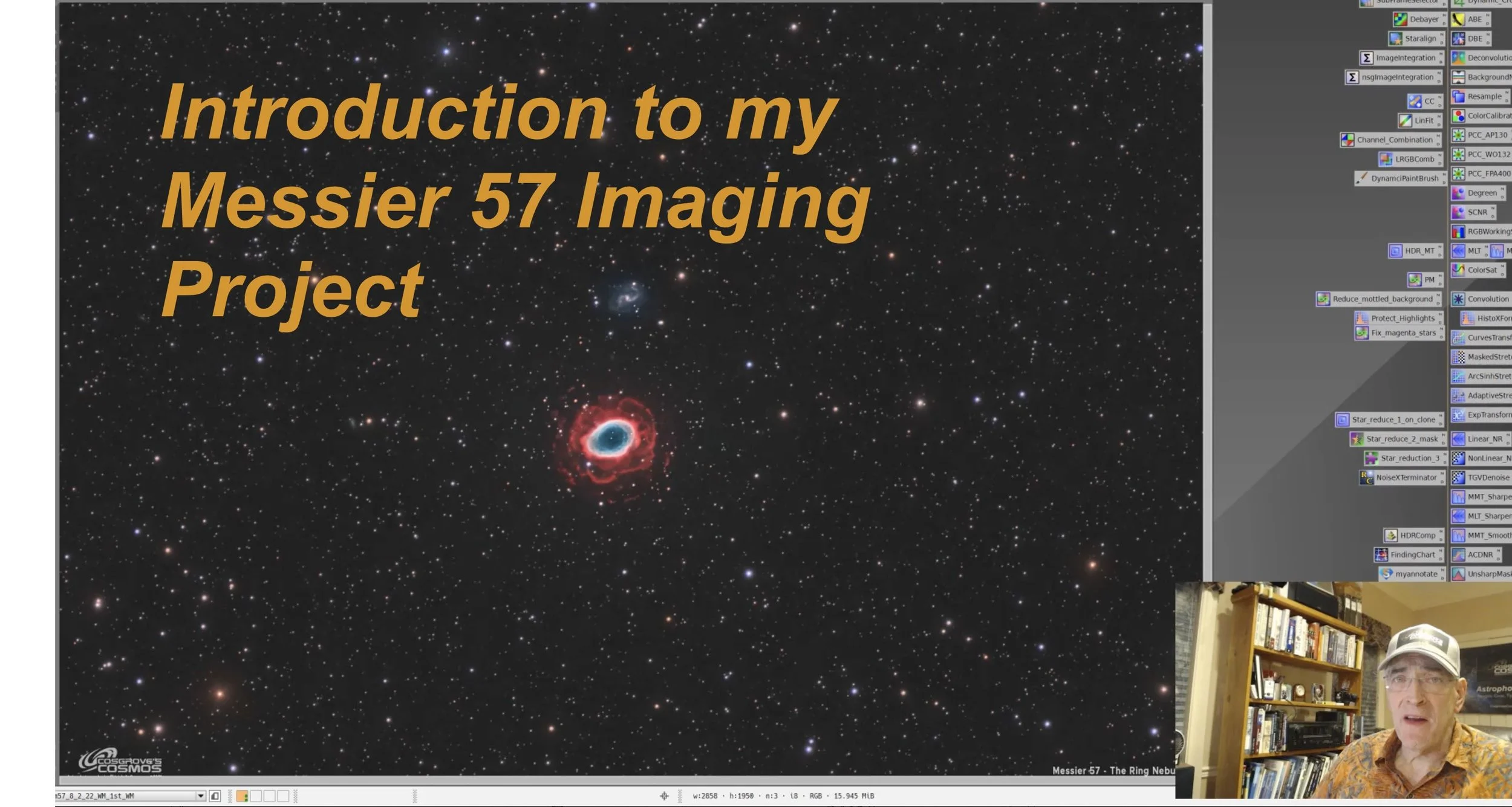
A new feature for Cosgrove’s Cosmos - A video introduction to the imaging project!
Target Selection
Every amateur astronomer with some kind of telescope has observed the Ring Nebula. Though small in angular size, it is relatively bright and easily located in the sky between the stars Beta and Gamma Lyrae.
I know I have observed it many times in my younger days when visual work was all I could really do. I remember the first time I saw its distinctive ring form, slightly oblong and with a dark hole in the center. This is a very cool target for a modest telescope!
In fact, at one time, I lived in Greece, NY - which was very light polluted.
I had just gotten an 8” Meade SCT, and I wanted to see the Ring Nebula. I had the scope lined up for where the object should be found and had chosen a low magnification eyepiece, so I had a slightly wider field of view to spot it more easily. But I saw nothing at all!
I had also just gotten a Lumicon O-III UHC visual filter, so I tried holding the filter between the eyepiece and my eye. To my amazement - when I flipped the filter in front of my eye, I could plainly see the nebula! When I removed it, it was gone! Right then and there, the O-III filter paid for itself!
This time of year, M57 is well placed for me, and I can get about 4 hours a night as it rises and moves between my treelines.
While I have shot M57 before (more about that in a minute), I decided that I wanted to try it again and do as long of integration as possible, and I also wanted to capture Ha data along with the LRGB data.
I have heard that long exposures with Ha data will show a set of outer shells of expanding gas that you don’t see visually, nor do you see this feature in most images of M57.
I have seen some incredible images of these outer rings. The one below was taken on a 2-meter Ritchey–Chrétien telescope located in the Canary Islands:

Göran Nilsson & The Liverpool Telescope:
HaRGB image of The Ring Nebula (M57) showing the faint outer shells. Data from the Liverpool Telescope (a 2 m RC telescope on La Palma) was processed by Göran Nilsson. 67 exposures totaling 1.9 hours. (Image taken from Wikipedia)

The building housing the Liverpool Telescope (taken from Wikipedia)
These images are often taken on massive professional telescopes and are super impressive!
Could I capture some of that detail with a 5” telescope taken from my driveway in the relatively poor skies of Rochester, NY? I was about to find out!
Previous Efforts
After having observed M57 over the years in many telescopes, it should not be surprising that I would want to capture M57 with the camera. I have shot this target twice in the past. The first one was in 2019- shortly after I started attempting astrophotography for the first time - and the second was in 2020.
The 2019 image can be seen HERE.
The 2020 image can be seen HERE.
Below are the the two images shown here for your convenience.
This very early image in my portfolio was taken in August of 2019. No exposure data was recorded at the time.
This image was taken in June of 2020, and is the result of 3.1 hours integration with an OSC camera.
The first image is pretty rudimentary. You can identify it as M57, but, in truth, it was an awful image. Of course, at the time, I was on cloud nine and shared this widely with family and friends, and on Facebook!
The 2020 version is much better. while it is still very a very small object for my telescopes, The fine detail and subtle colors are all there and all accurate. However, there is really no hint of the outer gas rings.
Data Capture
We have had an unusually warm and dry summer so far. As we entered the best portion of the lunar cycle for astrophotography, the weather predictions were looking strangely positive. Usually, such a promising weather prediction is just a cruel jest - typically, my hope fades as the clouds begin to roll in - along with waves of utter frustration. But this time the weather held! The nights were mostly clear and cool, with gentle winds and NO bugs to speak of! These were very pleasant nights!
I was able to image for a total of 5 nights: July 28,-July 31, and Aug 2. This in itself is remarkable. Three clear nights is more typical - maybe four if I get very lucky!
I typically set up my gear in the driveway while it is still light out. This takes me about 20 minutes to set up all 3 scopes. Then I wait until it is dark enough for the PA camera to see the stars around Polaris. For these nights - that was about 9:30 pm. Then I go out and do a polar alignment on all three scopes. This also takes about 10-15 minutes.
At that point, I fire up the camera, do a GOTO with the mount towards some bright star towards the South, and then do a platesolve. This calibrates the pointing on the telescope mounts. I then slew to the target and wait to start. I have to wait for:
the camera to come to the target temperature
targets to clear the tree line
true astronomical darkness to arrive.
For M57, I started the subs around 10 pm when it was close to astronomical darkness.
I then ran these until around 4 am - before twilight began. At that point, I would shoot flats and flat darks for the evening.
I collected over 17.25 hours of data - this is the longest integration I have ever achieved from my driveway! This was due to the convenient positioning of M57 - running diagonally between my tree lines, giving me the max time I can get in this locale. And also to the fact that I got 5 whole nights of clear skies!
Data Analysis
When I blinked the images, they looked great - only a small handful of subs were eliminated for one reason or another. (Note: I made videos of the blink reviews, which can be seen in the processing walkthrough below.)
So I loaded up the data into WBPP and did a full run that would do calibration, alignment, and integration - including drizzle processing.
This took about two hours to complete. When I looked at the resulting master images - I was disappointed - as the bright stars seem to have large haloes around them. Hmm.
So I went back and ran Subframe Selector on the registered images. I found that a surprising number of frames had very high FWHM star measures - especially on night two. Apparently, I had some very thin clouds come through - so thin that I could not see them during the blink process but enough so that the brighter stars were bloated and showed halos.
So I used SubFrameSelector to cull frames that had the worst impact. This resulted in the loss of 2.5 hours of integration - OUCH!
My 17.2 hours was now down to 14.7 hours!
I re-ran ImageIntegration to create new masters. These new masters looked much better - but not perfect.
Image Processing
When it was time to process the images, I tried two approaches.
For the first, I used starnet2 to create a star and starless images of the nonlinear RGB, L, and Ha images. I then processed these separately to reduce star sizes while still aggressively stretching the nebula images. This did not seem to work out for me, as I ended up with some artifacts around the stars.
While in theory, going the starless route should provide the best results. You stretch the nebulae that need to be enhanced and avoid doing that level of stretching on the stars. You have the best of two worlds when you reassemble the star and the starless image.
However, sometimes changing the star and starless images causes some artifacts where the stars and the backgrounds meet. I cannot always predict when this will happen. I have used this on many images and gotten great results.
But on this image, I had artifacts I could not resolve. So instead, I used my normal LRGB workflow and then folded in the Ha data along with a targeting mask. This seemed to work much better and was the approach taken for the final image.
When dealing with some of the bloated stars, I hoped my GOTO star reduction method - EZ-Star Reduction - would help reduce the still bloated bright stars. I ran it, and to my dismay - it ended up creating dark halo artifacts that I had not run into before. This seemed to be caused by the incomplete mapping of where the star edges were compared to the halos around those stars.
So I forced myself to try a new star reduction method recently released by Bill Blanshan. I was really glad I did. These new methods were easy to install, easy to use, super fast to run, and did an excellent job! This is a super elegant piece of work - thank you, Bill!
Details on this can be seen in the processing section below. You can also click HERE to see a video overview of the methods.
Final Results
I was very happy with my final image.
I have successfully captured the outer Ha expanding shell detail! While it is certainly not in the same realm as what is being done with 2-Meter diameter professional telescopes - for a driveway-based 5” scope - I think it came out quite well.
My one regret is that I don’t think the image is as sharp as it could be. For this, blame the thin clouds. But having said that, I was really happy to have had things come together (thank you, weather gods!), and I am always happy when the final image looks pretty cool!
A detailed Processing Walk-Through is provided for this image at the end of the posting…
More Information
Wikipedia: Messier 57
Nasa.gov - The Hubble Messier Catalog: Messier 57
messier.objects.com: Messier 57
The.Skylive.Com IC 1296
Cambridge-Photographic-Atlas-of-Galaxies: IC 1296
Capture Details
Lights Frames
Data was collected over five nights: July 28,-July 31, and Aug 2.
73 x 90 seconds, bin 1x1 @ -15C, Gain Zero, ZWO Gen II Lum filter
98 x 90 seconds, bin 1x1 @ -15C, Gain Zero, ZWO Gen II Red filter
101 x 90 seconds, bin 1x1 @ -15C, Gain Zero, ZWO Gen II Green filter
102x 90 seconds, bin 1x1 @ -15C, Gain Zero, ZWO Gen II Blue filter
63x 300 seconds, bun 1x1, @ -15C, Gain Zero, Astronomiks 6mm Ha filter
Total of 14.7 hours
Cal Frames
25 Darks at 90 seconds, bin 1x1, -15C, gain Zero
25 Darks at 300 seconds, bin 1x1, -15C, gain Zero
12 Flats at bin 1x1, -15C, gain Zero - for LHaRGB filters.
25 Dark Flats at Flat exposure times, bin 1x1, -15C, gain unity
Software
Capture Software: PHD2 Guider, Sequence Generator Pro controller
Image Processing: Pixinsight, Photoshop - assisted by Coffee, extensive processing indecision and second-guessing, editor regret, and much swearing…..
Capture Hardware:
Scope: Astro-Physics 130mm F/8.35 Starfire APO
built in 2003
Guide Scope: Televue TV76 F/6.3 480mm APO Dublet
Main Fous: Pegasus Astro Focus Cube 2
Guide Fous: Pegasus Astro Focus Cube 2
Mount: IOptron CEM60 - new
Tripod: IOptron Tri-Pier with column extension
Main Camera: ZWO ASI2600MM-Pro
Filter Wheel: ZWO EFW 7x36
Filters: ZWO 36mm Gen II LRGB filters
Astronomiks 36mm 6nm Ha, OIII, & SII filters
Rotator: Pegasus Astro Falcon Camera Rotator
Guide Camera: ZWO ASI290MM-Mini
Power Dist: Pegasus Astro Pocket Powerbox
USB Dist: Startech 7 slot USB 3.0 Hub
Software:
Capture Software: PHD2 Guider, Sequence Generator Pro controller
Image Processing: Pixinsight, Photoshop - assisted by Coffee, extensive processing indecision and second-guessing, editor regret and much swearing…..
Click below to see the Telescope Platform version used for this image
Image Processing Walk-Through
(All Processing done in Pixinsight - with some final touches done in Photoshop)
1. Blink Screening Process
Lum subs
Trails - but all looks good. No gradients
Red subs
Lots of trails. Very minor gradients
3 frames removed for cloud cover issues - from night 5
Green subs
6 removed for clouds - from night 5
Fewer trails, Minor gradients
Blue subs
1 removed for clouds
Very minor trails
Ha subs
No frames removed
Very minor trails and gradient
Flats
All flats looked good
Dark flats
Lum 0.08 sec - good
Red 0.43 sec - good
Green 0.23 sec - good
Blue 0.19 sec - good
Ha 12.78 sec - good
Darks
Get 90-second Darks from Calibration files from the recent M13 project
Get 300-second Darks from the M101 project
Below you can see videos of the Blick runs. Note that at the end of each video, you can see a “+” symbol curving across the screen - this is an artifact of the screen recording mode when I moved the cursor to stop the recording.
2. WBPP 2.4.5
Note - I intended to load all data into WBPP and use it to control the entire process, including drizzle processing and integration. However, I had an issue with the results, which caused me to redo the integration. More on this later in the notes. For now - this is how I set up and ran WBPP.
The panel was completely Reset
All lights loaded
All darks and flats loaded
CC set up and enabled for all filters
Ha pedestal image - auto mode enabled.
Drizzle processing enabled
Integration enabled
Linear normalization set for Auto and for the best group of frames
Ran with no problems - Done in 2 hours

WBPP Calibration view.
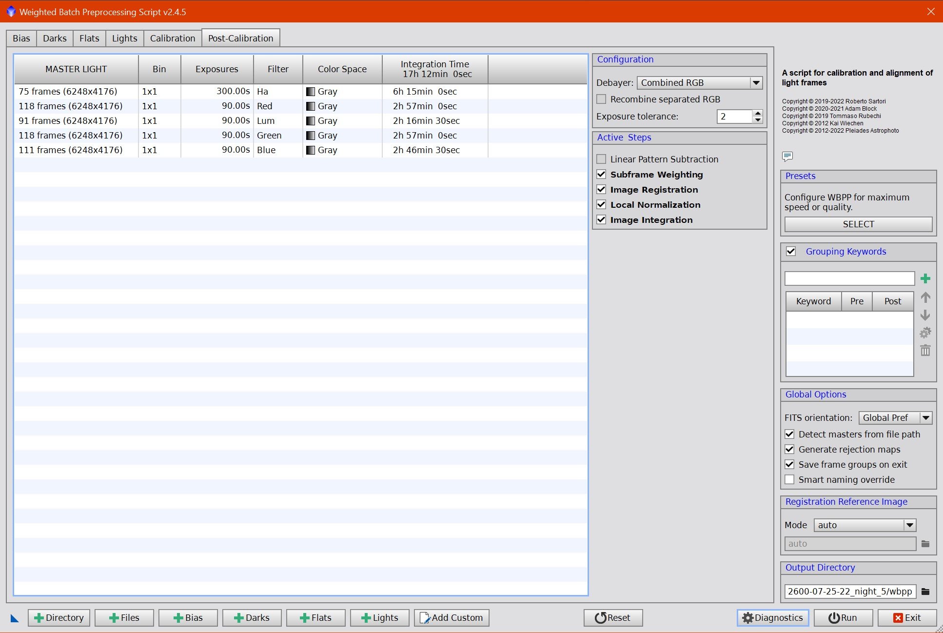
Post Calibration View.
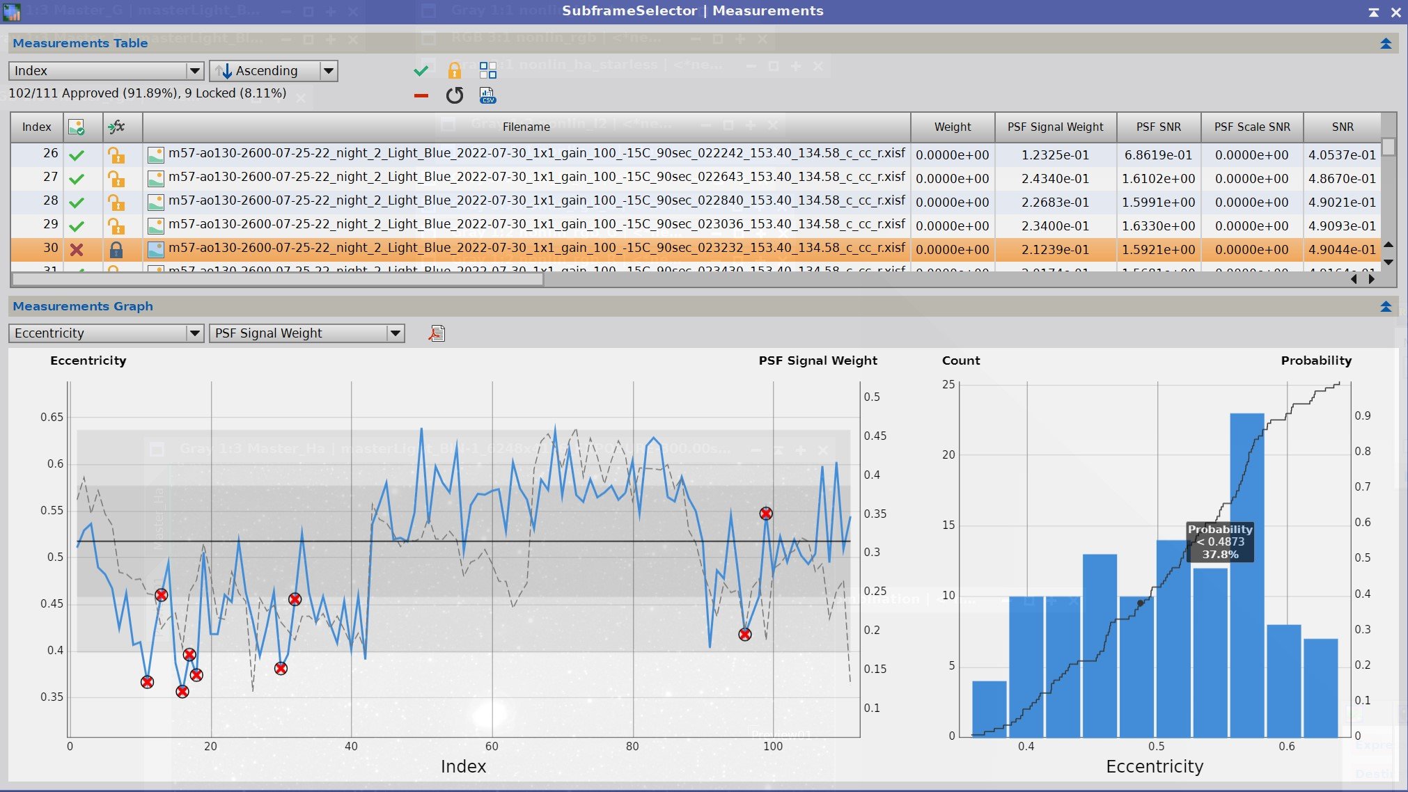
3.0 Use SubFrameSelector to analyze the Calibrated subs
After WBPP ran, I looked at the Master images and was not pleased with what I saw. There was significant star bloat and halos around the brighter stars. To understand what happened, I ran SubFrameSelector on each of the Registered frames for each filter, and based on what I saw there, I took the action of culling more subs from the data.
Subs for each filter were loaded into the tool, and metrics were computed. FWHM and Eccentricity were the key metrics I used in this analysis. Screenshots for each filter are attached below.
Lum Images: 18 deleted for having either too high an FWHM or Eccentricity value
Red Images: 20 deleted for having too high an FWHM or Eccentricity value
Green Images: 17 deleted for having too high an FWHM or Eccentricity value
Blue Images: 9 deleted for having too high an FWHM or Eccentricity value
Ha images: 11 deleted for having too high an FWHM or Eccentricity value
I was pretty aggressive on what I eliminated. A total of 2.5 hours of integration was thus lost.

Lum Sub FWHM - Note eliminated frames

Red Sub FWHM - Note eliminated frames

Green Sub FWHM - Note eliminated frames

Blue Sub FWHM - Note eliminated frames

Ha Sub FWHM - Note eliminated frames

Lum Sub Eccentricity - Note eliminated frames

Red Sub Eccentricity - Note eliminated frames

Green Sub Eccentricity - Note eliminated frames
Blue Sub Eccentricity - Note eliminated frames

Blue Sub Eccentricity - Note eliminated frames
4. Integration
ImageIntegration
ImageIntegration was run for each Master image.
It used the same setup for each run.
ESD was chosen for rejection.
Large scale rejection checked - 2x2
A sample panel for ImageIntegration can be seen below

ImageIntegration panel settings.
Rejection High - Lum: Note trails removed (click to enlarge)

Rejection High - Green: Note trails removed (click to enlarge)
Rejection High - Ha: Note the lack of trails! (click to enlarge)
Rejection High - Red: Note trails removed (click to enlarge)

Rejection High - Blue: Note trails removed (click to enlarge)
5. Crop all of the images
A common crop level was selected, and DynamicCrop was used to trim all of the master frames.
A substantial crop was made to highlight Messier 57 and the small barred-spiral galaxy just above it. This crop can be seen below.
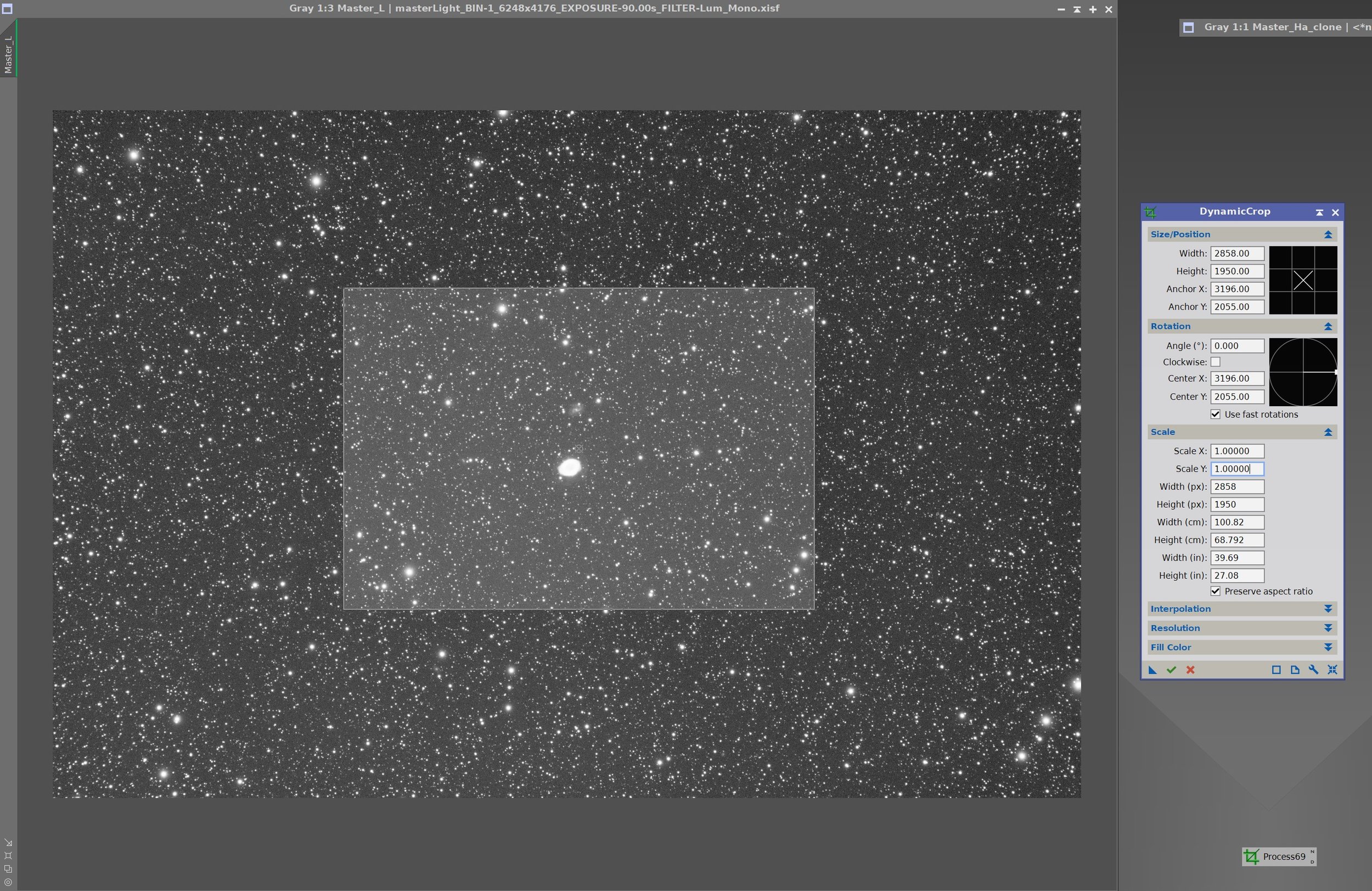
The significant level of crop used for this image.
6. Dynamic Background Extraction
DBE was run for each image using the subtraction method. Below are the Sampling plans, the before image, the after image, and the removed background images.
DBE: L Sampling (Click to enlarge)
DBE: R Image Sampling (Click to enlarge)
DBE: G Sampling (Click to enlarge)
DBE: B Sampling (Click to enlarge)
DBE: Ha Sampling (Click to enlarge)
L image Before DBE (click to enlarge)
R Image Before DBE (click to enlarge)
G image Before DBE (click to enlarge)
B image Before DBE (click to enlarge)
Ha image Before DBE (click to enlarge)
L image After DBE (click to enlarge)
R Image After DBE (click to enlarge)
G Image After DBE (click to enlarge)
B image After DBE (click to enlarge)
B image After DBE (click to enlarge)
L background removed (click to enlarge)
R background removed (click to enlarge)
G background removed (click to enlarge)
B background removed (click to enlarge)
Ha background removed (click to enlarge)
7. Create and Process the Linear Color Image
Use ChannelCombination process to create an initial RGB image.
Run PCC to color calibrate the image
Run Noise XTerminator with a value of 0.5 to “knock the fizz off”
Initial RGB Linear Image (click to enlarge)

PPC was run and the following balance function were computed.
After PCC applied. (click to enlarge)
Before and After application of RC Noise XTerminator with a value of 0.5
8. Process Lum and Ha Nonlinear Images
Prep for Deconvolution
Create a PFS-Lum image by running PFSImage Script
Create LDSI image
Run Starmask process with parameters seen in the screen snap below
Run HT to boost the resulting star mask using the HT curve seen in the snap below
Select a few image previews for testing deconvolution parameters
Run Deconvolution using the PFS image and the LDSI Image - iteratively test parameters until the best result is obtained.
see final parameters below.
Run Noise XTerminator with a value of 0.55
Repeat this process for the Ha image.

PSFImage Panel for the Lum image.

The Lum PSF image

Stramsk setting used to create original LDSI map

HT transform to boost LDSI map
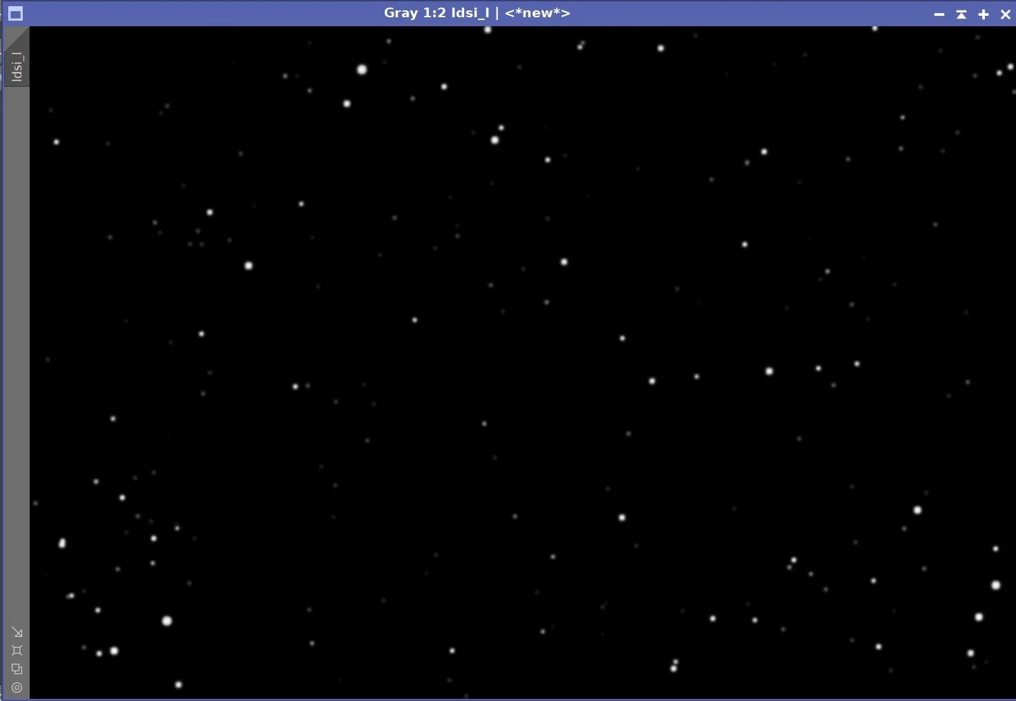
The final Lum LDSI image.

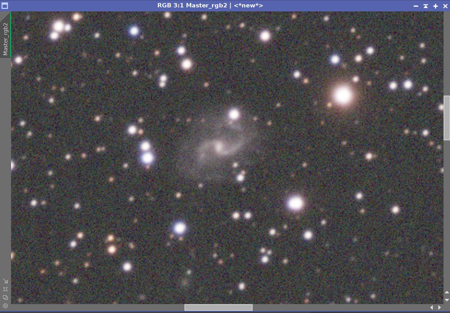
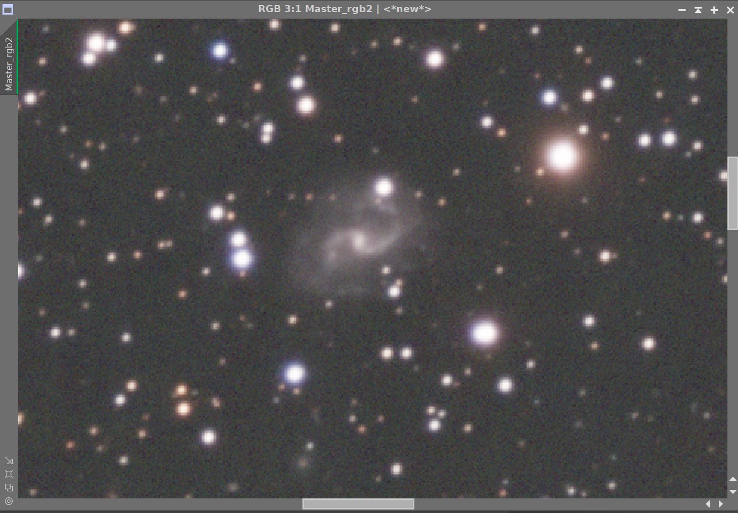
The two preview regions set up to explore decon settings for the Lum image
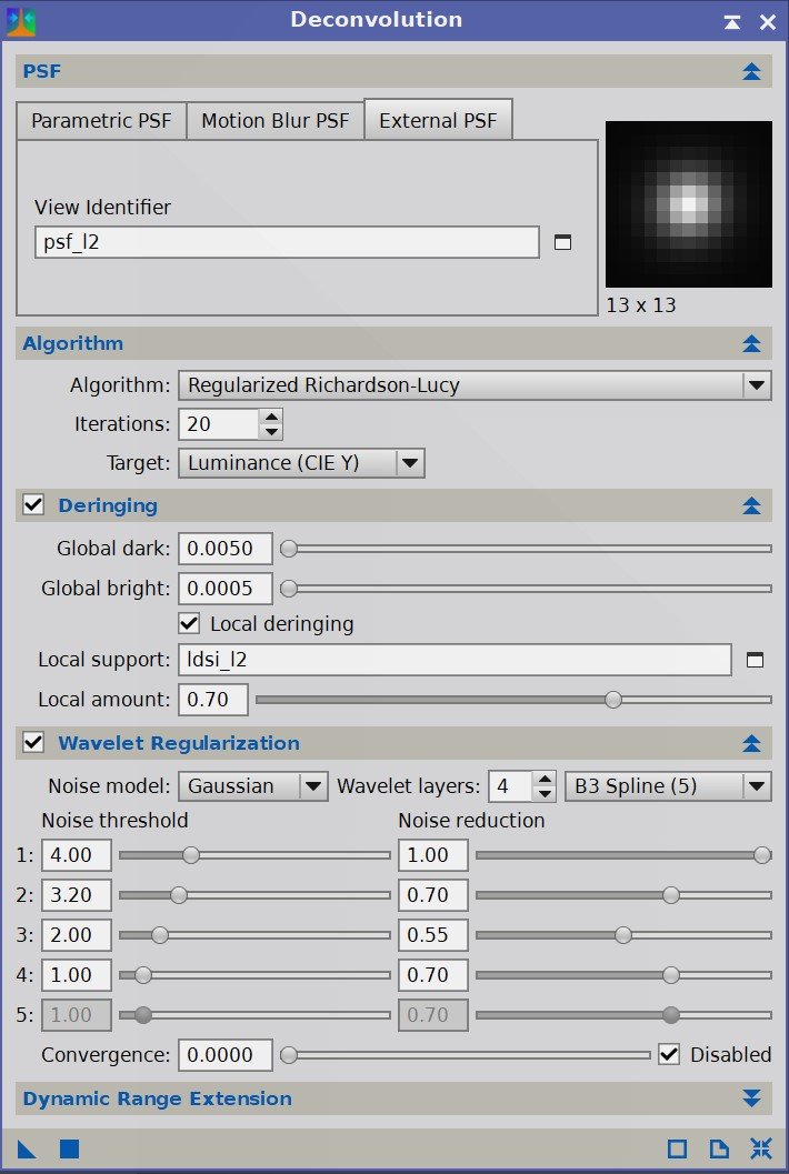
The final settings on the Decon Panel for the Lum image.

Lum Image Before and After Deconvolution, and After Noise XTerminator 0.55

The PFSImage Panel for the Ha image.

The Final PSF image for Ha

The LDSI image for Ha

The previews selected to test Decon parameter values for the Ha image.

The final Deconsolvution panel settings for the Ha image.
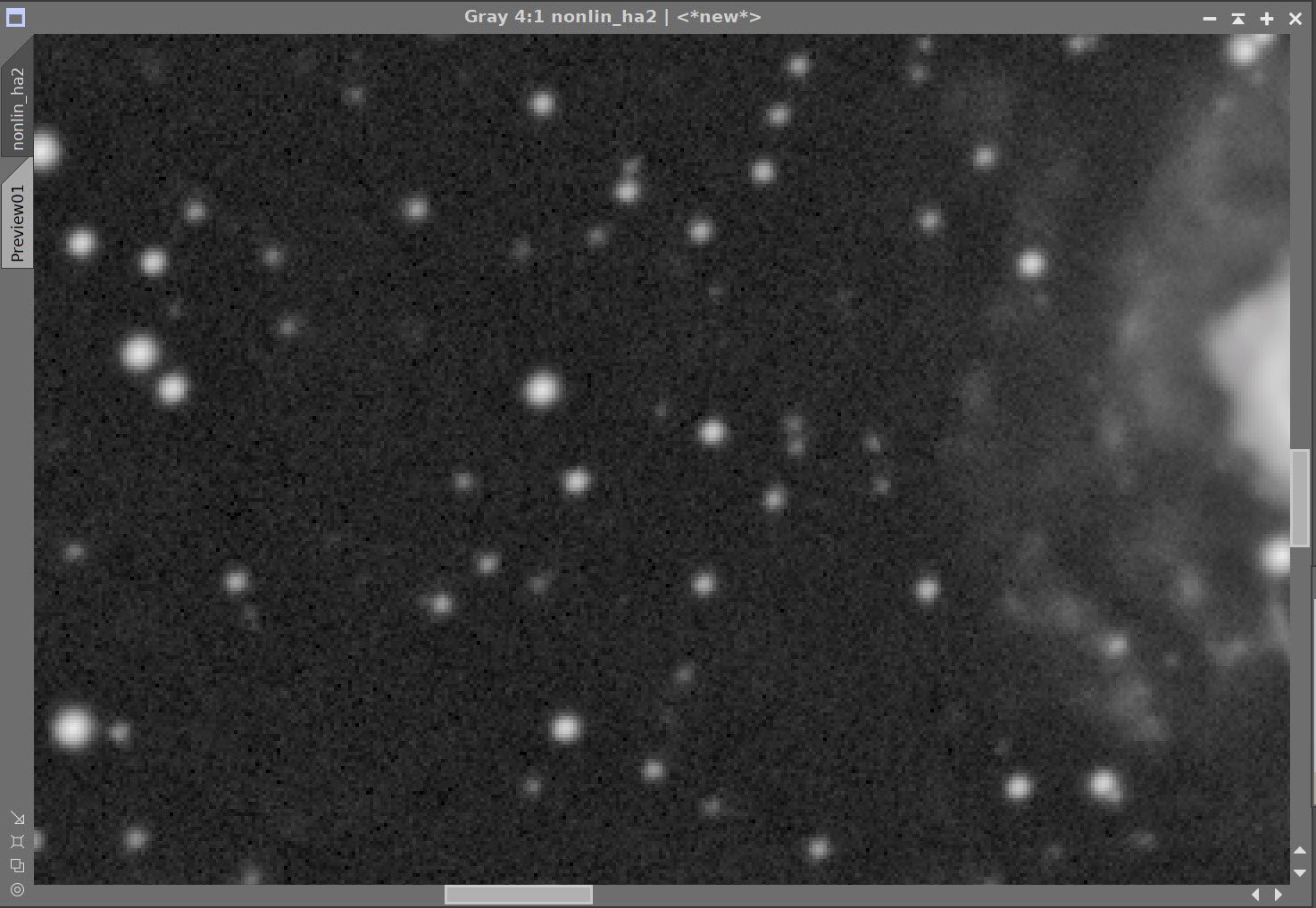
Ha Image Before and After Decon, and aft Noise XTerminator 0.5
9. Take the Lum and Ha image Nonlinear.
For the Lum image:
Create a Preview of a good sample of the background sky
Run MaskedStretch on the image - using the sky background preview as a reference.
Use CT to adjust Tonescale
Run HDR-MT with a level of 5
Create a mask covering M57 with the GAME script
Apply this mask to the image
Run HDR-MT with a level = 4
Run CT and tweak the tone scale for the local region of M57
Remove Mask
Run CT and tweak the global tone scale
Run Noise XTerminator at 0.5
For the Ha image:
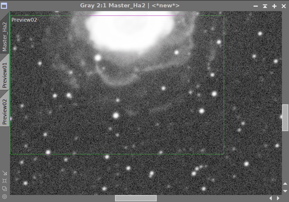
Create a Preview of a good sample of the background sky
Run MaskedStretch on the image - using the sky background preview as a reference.
Use CT to adjust Tonescale and Run HDR-MT with a level of 5
Run Noise XTerminator with value of 0.55
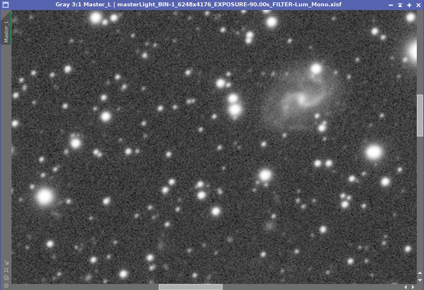
Lum image after MaskedStretch (click to enlarge)

Mask covering M57 created with the GAME script
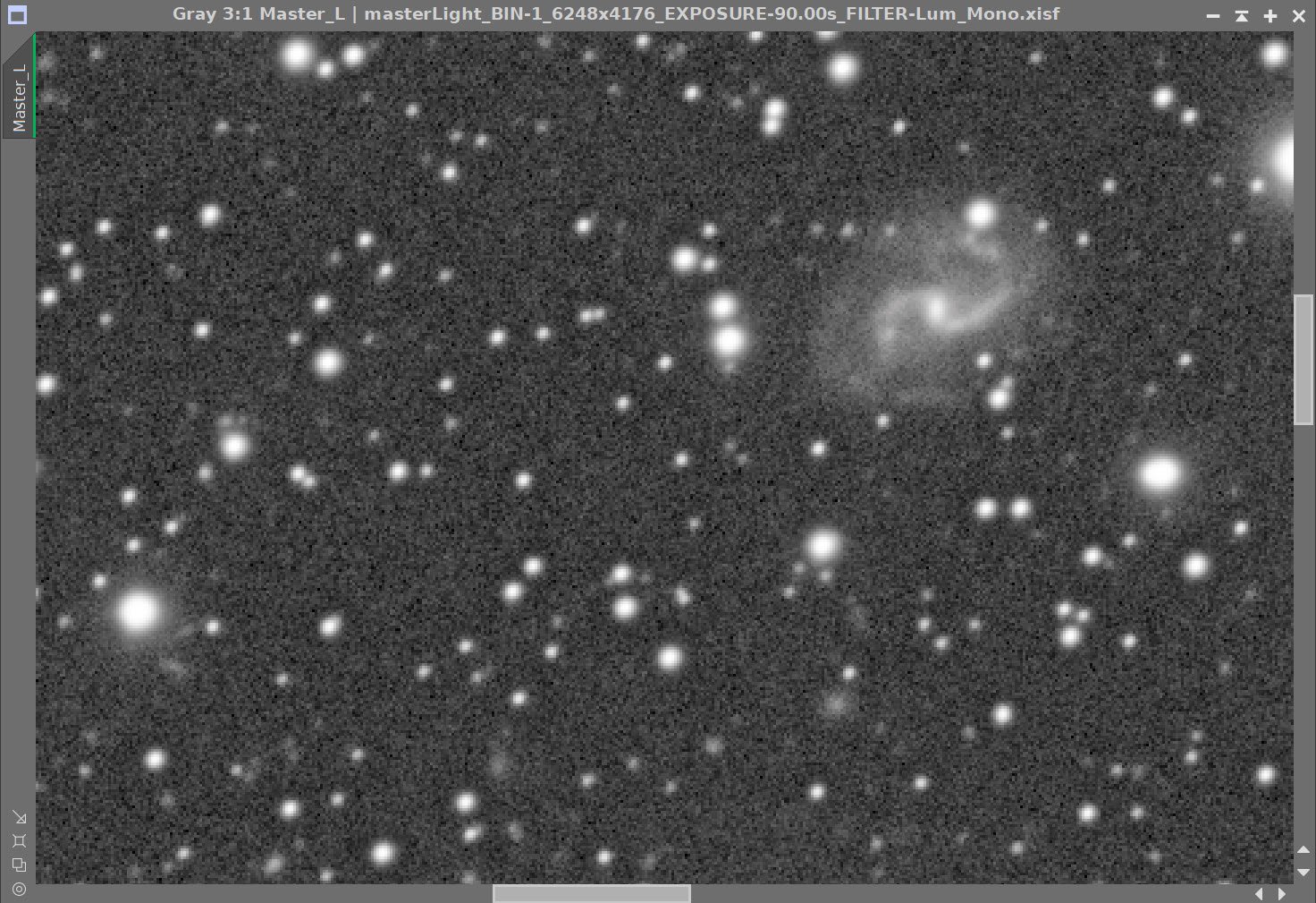
Lum image after HDR_MT (click to enlarge)
After HDR-MT applied with the GAME mask (click to enlarge)

After final CT adjustments.
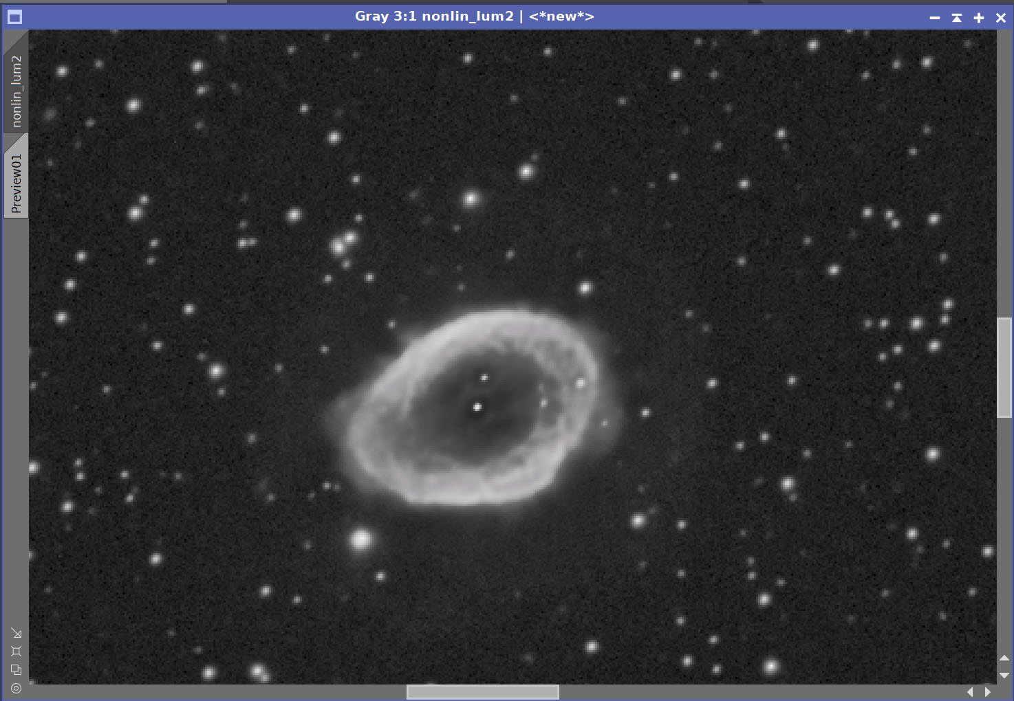
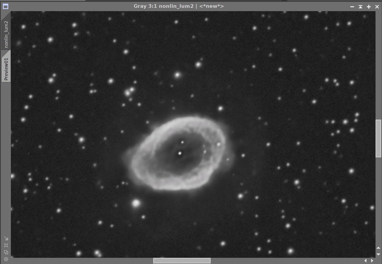
Nonlinear Lum image - Before and After Noise XTerminator 0.5

The Final Nonlin Lum Image
Now for the Ha image…
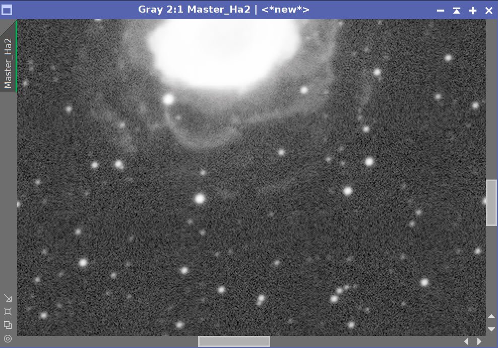
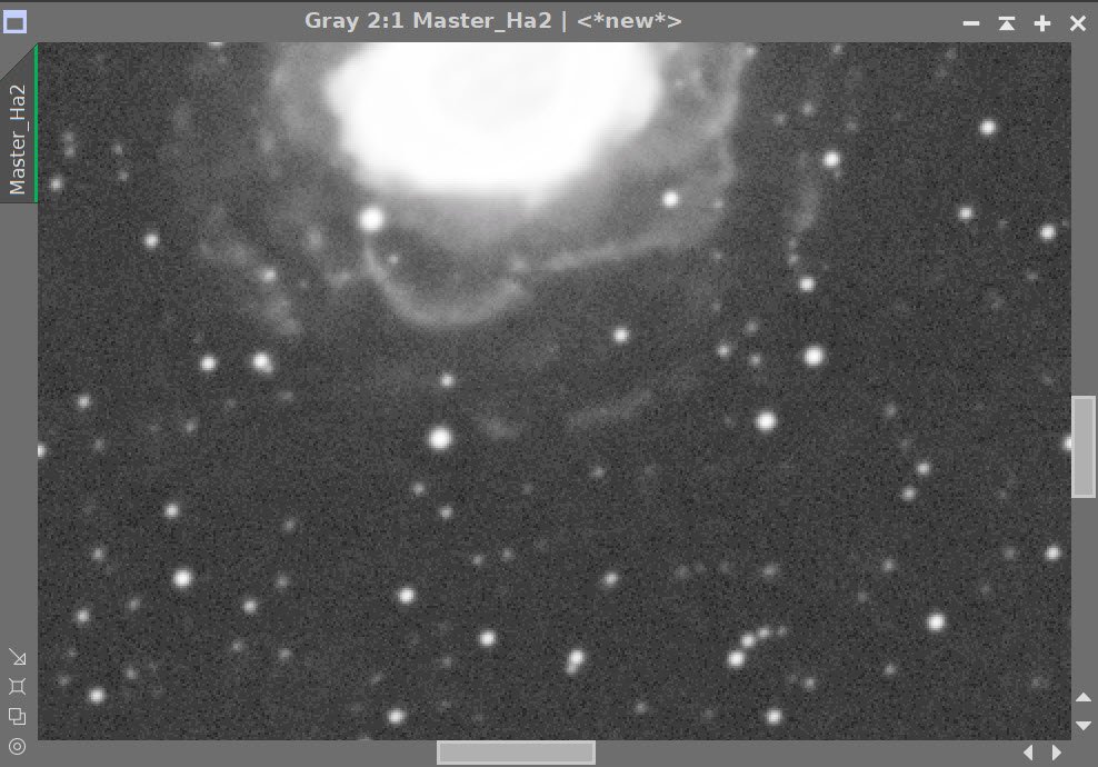
Initial Nonlinear Ha image after a Masked Stretch. (click to Enlarge)
Nonlinear Ha image after HDR-MT with levels = 5 applied (click to enlarge)

Before and After Noise XTerminator 0.5

The FInal Ha image
10. Take Linear RGB Image Nonlinear
Select a Preview for a good sampling of the background sky.
Run MaskedStretch, using the above background preview.
Run CT and adjust color sat and tone scale
Run HDR-MT with level = 3
Run LHE radius = 64, contrast limit = 2.0, amount= 0.5, 8-bit histogram
Nonlinear RGB image after MaskedStretch and CT used to adjust tone scale and color sat. (click to enlarge)
After HDR-MT level - 3 run. (click to enlarge)
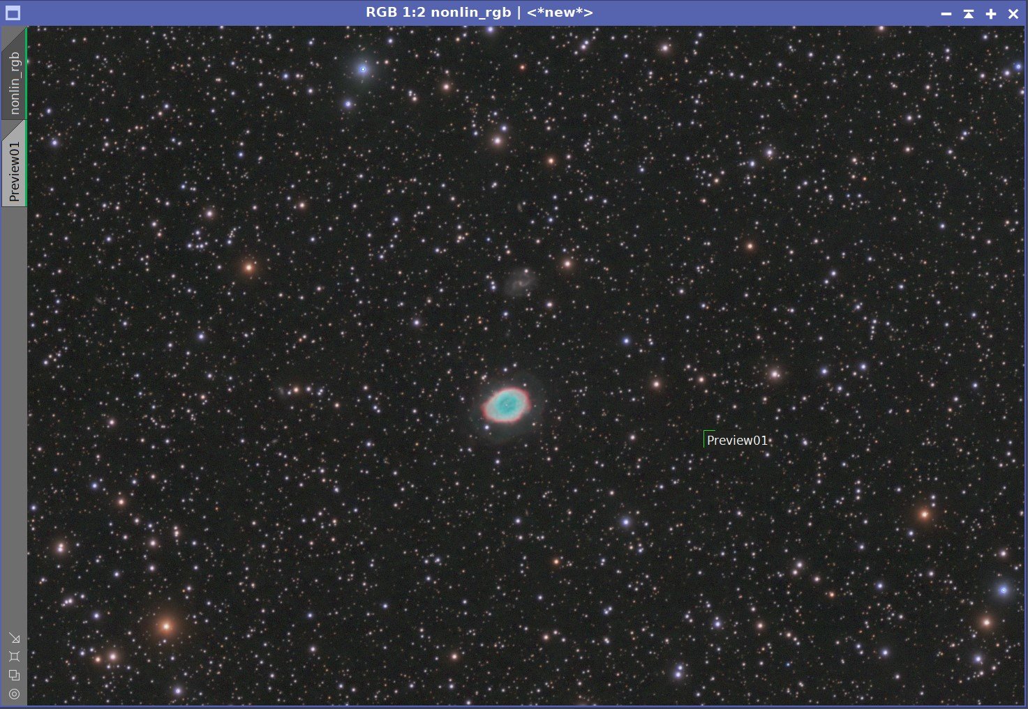
After LHE is run - The final RGB image.

The three primary nonlinear images, ready for combination: Lum, RGB, and Ha.
11. Final combination and processing of the non-linear RGB image
Use LRGBCombination to create the LRGB image
Run CT to adjust tone scale and color saturation
Apply the M57 GAME Mask
Apply CT - tweak the color and tone scale of just the nebula
Apply ColorSaturation - selectively adjust color sat of various hues
Create A Ha region mask
Use the RangeSelection to include most of the Ha outer rings
Use the DynamicPaintBrushtool to remove everything from the mask but the Ha rings
Use CT to boost the contrast of the mask region
Insert Ha ring content
apply Ha Region Mask
Use PixelMath to add the Ha image to the red channel, while keeping the Green and Blue Channels the same. See snapshot of the PM panel below to see the weighting used.
The initial LRGB image after Lum insertion (click to enlarge)
After a quick CT run to adjust color sat and tone scale (click to enlarge)
With the M57 GAME Mask applied, adjust CT and run ColorSaturation to finalize the color and tone scale. (click to enlarge)

The first step in creating the Ha Region Mask is to use RangeSelection to create an initial range mask. (click to enlarge)
Next, the DynamicPaintBrush is used to remove all features from the mas that are not part of the outer rings. (click to enlarge)
FInally - CT is applied to boost the features of the HA region mask (click to enlarge)

Using Green = $T[1], and Blue = $T[2], use the weighting equation above for the Red channel. Apply the Ha region mask and drag this onto the LRGB image.

The initial LHARGB image
12. Star Reduction
Because of the thin cloud-induced star bloat, this image really needs star reduction.
My goto process for dong this is EZ-Star Reduction using the Adam Block method. So I ran that and ended up with the following before an after image:
before EZ-Star Reduction (click to enlarge)
After EZ-Star Reduction (click to enlarge)
At first look, things look good - a substantial amount of Star Reduction has been achieved! However, when I looked closer, I found some strange dark halo artifacts around the largest and most bloated stars:

Dark halos around bloated bright stars after EZ-Star Reduction.
This was not acceptable. It would seem that the reduction region was not large enough to include all of the halos, resulting in these dark halos.
This result caused me to try out a new set of Star Reduction methods that were created and recently released by Bill Blanshan. These add four new instances to your desktop process icons:
One makes it easy to create a clone image with a standard name: “Starless”, you then run your favorite str removal algorithm on this clone image.
Method 1
Method 2
Method 3
These methods are run in PixelMath and are super fast. They produce great results that are easy to customize to your preferences. I am really liking what Bill has done here!
Here are three example images processed with the three methods, with the strength dialed down a bit.

Method 1, S = 0.25

Method 2, S=0.25

Method 3, 1 & 3
For me, I chose method #2 with an S value of 0.35. This helped greatly. The brighter stars still have some bloat, but my plan is to selectively adjust them further in Photoshop using the RC Starshrink tool.
Before Star Reduction (click to enlarge)
FInal Image after Blanshan Star Reduction
13. Export to Photoshop
Save images as Tiff 16-bit unsigned and move to Photoshop
Use Camera Raw Filter to adjust Global Clarity, Texture, and Color Mix
ColorMix is much easier to use to adjust hues in an image compared to the tool provided by Pixinsight, and I tend to do this final operation in PhotoShop
Use StarShrink to reduce just the largest stars further. This further helps the bloat.
Use a lasso with a feather of 25 pixels to select areas around the Ha rings
Use camera Raw to enhance the brightness and clarity
Use Noise XTerminator to soften noise
Use a lasso with a feather of 25 pixels to select the small galaxy
use the camera raw filter to adjust charity and texture and color grading to bring out high-end vs low-end color.
Use Noise XTerminator to soften the noise pattern.
Add watermarks
Export Clear, Watermarked, and Web-sized jpegs.

The final image.
Adding the next generation ZWO ASI2600MM-Pro camera and ZWO EFW 7x36 II EFW to the platform…