At the CIMSS Satellite Blog, we occasionally get emails from our readers. Yesterday’s (6 February 2024) email included this one:

I was doing some forecasting for the Canadian Arctic today and noticed a very
impressive blowing snow signature on satellite; not that blowing snow is
uncommon up there, but rather that the signature was so strong given the lower
resolution and parallax at that latitude.

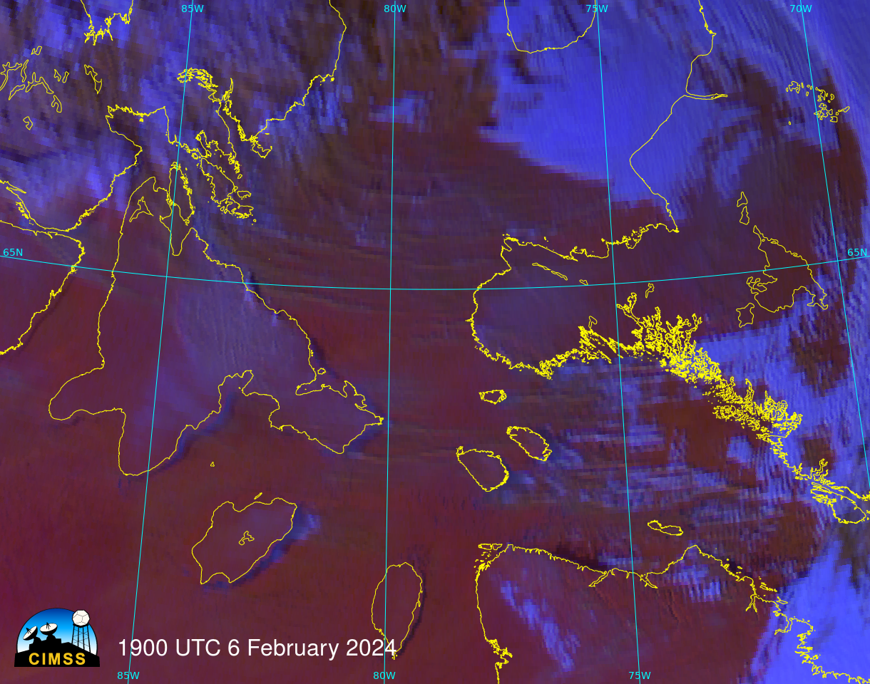
The email included this link to the CIRA SLIDER, where a Day Snow Fog image loop was displayed, including the frame below. The linear structures that appear in the RGB between, for example, Southampton and Nottingham Islands (here’s a map with islands labeled) are characteristic of blowing snow. (See this blog post for more information on RGB detection of blowing snow) Other linear features are north of Southampton Island.

This was happening south of strong storm (with a central pressure of 991 mb) even farther north than northern Hudson Bay, shown in the map below.

The Day Snow Fog Quick Guide (here, one of many Quick Guides developed over the years by scientists at CIMSS, CIRA and SPORT) describes the components of the RGB. I decided to create the RGB using CSPPGeo‘s geo2grid software, and the way to do that is to insert definitions into two different yaml files within the geo2grid file structure.

First, define the RGB in $GEO2GRID_HOME/etc/polar2grid/composites/abi.yaml by adding the lines below. I called this Day Snow Fog RGB ‘dsfog’: the ‘Red’ component is Band 3 (0.86 µm); the ‘Green’ component in Band 5 (1.61 µm); the blue component is a difference field, Band 7 – Band 13 (3.9 µm – 10.3 µm). When invoking geo2grid, the -p dsfog flag tells the software to create Day Snow Fog imagery.

  dsfog:
    compositor: !!python/name:satpy.composites.GenericCompositor
    prerequisites:
      - name: C03
      - name: C05
      - compositor: !!python/name:satpy.composites.DifferenceCompositor
        prerequisites:
        - name: C07
        - name: C13
    standard_name: dsfog

Then, assign bounds and gamma in $GEO2GRID_HOME/etc/polar2grid/enhancements/abi.yaml, shown below. Band 3 reflectance values range from 0 to 100, band 5 reflectance values range from 0 to 70, and the Band 7 – Band 13 brightness temperature difference ranges from 0 to 30^oC. In addition, a gamma of 1.7 is applied to each of the RGB bands.

  dsfog_abi:
    standard_name: dsfog
    name: dsfog
    operations:
      - name: stretch
        method: !!python/name:satpy.enhancements.stretch
        kwargs:
          stretch: crude
          min_stretch: [0.0, 0.0, 0.0]
          max_stretch: [100.0, 70.0, 30.0]
      - name: gamma
        method: !!python/name:satpy.enhancements.gamma
        kwargs:
          gamma: [1.7, 1.7, 1.7]

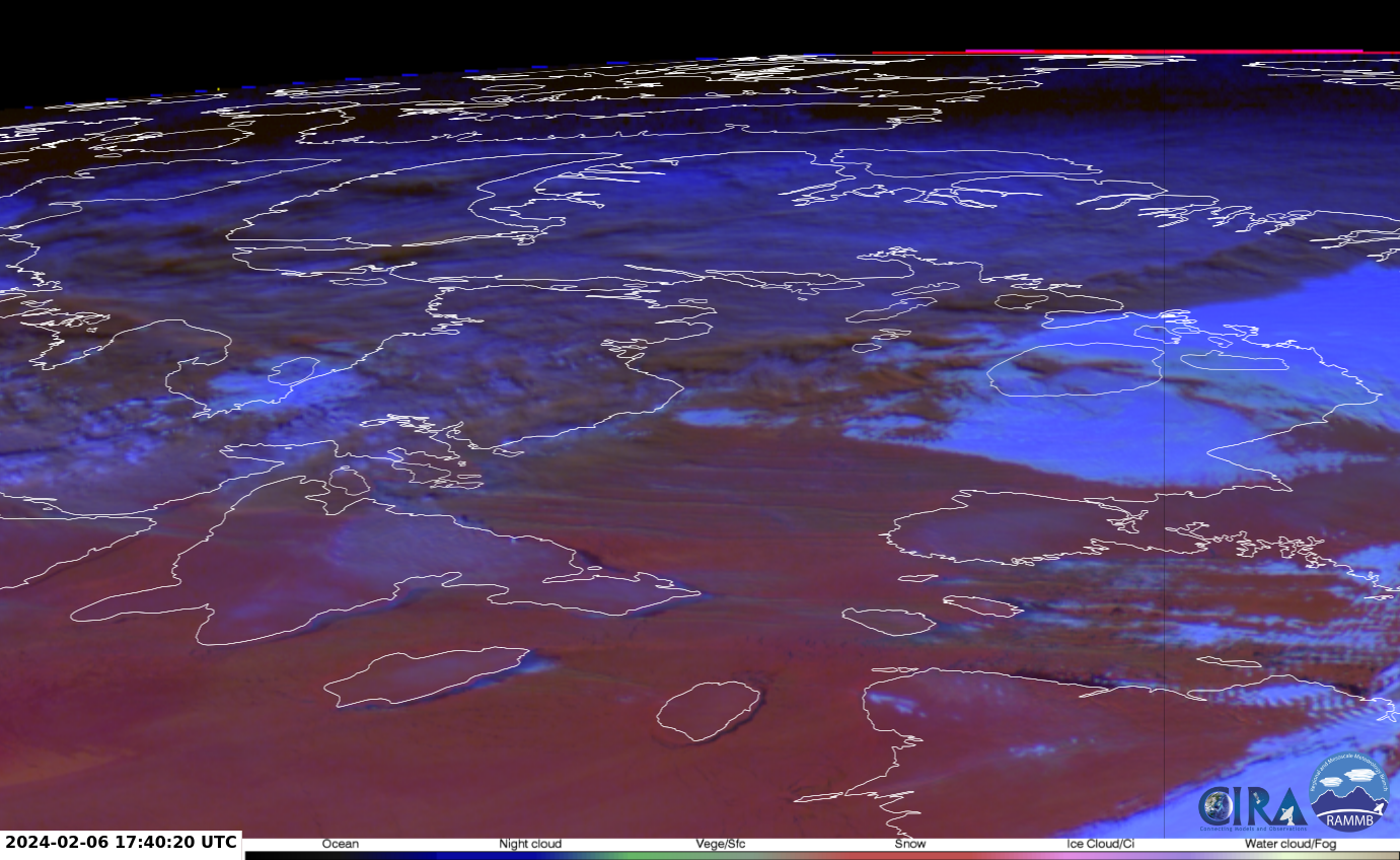
Use the p2g_grid_helper.sh shell script to define a grid (‘MyMap’, defined in ‘MyMap.yaml’ as used in the geo2grid call below) onto which data will be displayed. Then two geo2grid calls create the imagery and put georeferencing onto it. I used ImageMagick to annotate the imagery, and the animation is shown below. Characteristic linear features that are a bit greener than the underlying red surface show where blowing snow is occurring. In the absence of surface observations, this can give important information.

$GEO2GRID_HOME/bin/geo2grid.sh -r abi_l1b -w geotiff -g MyMap --grid-configs MayMap.yaml -p dsfog -f /path/to/goes16/abi/L1b/RadF/*s2024037[time]*
../add_coastlines.sh --add-coastlines --coastlines-resolution f --add-grid --grid-D 5.0 5.0 --grid-d 5.0 5.0 --grid-text-size 14 GOES-16_ABI*dsfog*.tif

---

Another (higher-contrast) version of the GOES-16 Day Snow-Fog RGB along with the Day Cloud Phase Distinction RGB was also created using Geo2Grid, as shown below. The higher-contrast RGB imagery depicted the areal coverage of horizontal convective roll clouds — which often highlight the presence of blowing snow — a bit more clearly as they streamed eastward from Southampton Island (and even Coats Island, just to the south). The higher contrast also helped to accentuate the polynyas that were slowly opening just downwind of the islands.

---

Thanks to Brad Vrolijk for alerting us to this far north event!

View only this post Read Less

Abundant convection over the southern Pacific Ocean has organized into a tropical cyclone (named Nat) as the system moved to the east of the Samoan Islands. GOES-18 infrared imagery, above, shows the strong convection that developed just east of Olosega; by 0700 UTC on 5 February 2024, very cold cloud tops (brightness temperatures cooler than -90^oC) appeared near 14^oS, 165^oW (shown here) as the system moved steadily to the east.

The tropical cyclone developed in a narrow ribbon of low shear values that have persisted for at least the 24 hours ending at 1200 UTC on 5 February, as shown in the analysis below from the CIMSS Tropical Cyclone page (direct link to product).

Sea-surface temperatures under the system are very warm, around 30^oC. The projected path, however, take the storm poleward towards cooler SSTs. In addition, the path takes the storm where observed shear values at present quite high.

MIMIC Total Precipitable Water fields (from this site), below, show a cyclonic spin developing just east of the Samoan Islands as the storm develops. A second invest area exists near 150 W, to the east of the Tropical Cyclone, and another tropical invest is near Vanautu at 160 E. (Click here).

The Regional Specialized Meteorology Center (RSMC) in Fiji (link) is issuing advisories on this storm, as shown below. The forecast path is towards the east-southeast towards 20^oS latitude. The Joint Typhoon Warning Center (link) is also issuing advisories (here is the 1500 UTC 5 February 2024 graphic). Some strengthening is forecast for 5-6 February, with slow weakening after that.

More information on this Cyclone is available at the CIMSS Tropical Website, at the JTWC and at the RSMC in Fiji.

View only this post Read Less

The Direct Broadcast antenna at the UW-Madison CIMSS can receive information over much of the contiguous United States. This includes the NOAA-20 overpass that acquired data around 0910 UTC over southern California during a frontal passage. NOAA-20 supports both the Visible Infrared Imaging Radiometer Suite (VIIRS) and the Advanced Technology Microwave Sounder (ATMS) instruments. Microwave imagery from ATMS, above, at 21.3 and 36.5 GHz, (from this temporary site) show the narrow stream of moisture flowing into southern California. Note the very cold brightness temperatures south of Baja California. In this region, clear skies are allowing information from the ocean surface to reach the satellite, but ocean water has very low emissivity at microwave frequencies/wavelengths; as a consequence, the computed brightness temperature (computed assuming a blackbody emission) is very cold.

Weighting Functions for ATMS Bands 18-22, below (source), show that Band 22 receives information from higher in the atmosphere and Band 18 received information from lower in the atmosphere. All five frequencies are within a region where microwave energy is strongly absorbed by water vapor (as shown in this absorption spectrum figure from here). You can infer from the weighting functions that Band 22 is a region where water vapor absorption is strongest of the 5 channels, and Band 18 is in a region of the spectrum where water vapor absorption is weakest of these 5 channels.

ATMS Brightness Temperatures for channels 18-22 are shown below. All show cooler temperatures over southern California (and in a band extending to the southwest of southern California). This suggests that water vapor is either more abundant in this region, or at higher altitudes (or both). These images give qualitative estimates of moisture. As noted above, the moisture band is fairly narrow.

MIRS software that is part of CSPP (software that is used at direct broadcast sites to process the signal from ATMS or VIIRS) can be used to create horizontal fields of temperature and dewpoint from the microwave information. These quantitative fields are shown below. The dewpoint fields show higher dewpoints that are especially concentrated at about 500 mb. A sharp northern edge to the moisture is also apparent.

MIRS temperature fields in the mid- to lower-troposphere, below, suggest a fairly sharp temperature gradient associated with the northern edge of the moist plume.

---

The I05 image (11.45 µm), below, from VIIRS, shows infrared information over southern California. The front affecting southern California is manifest as a relatively narrow band of cloudiness. Skies are mostly cloud-free south of Baja California. It’s easier to interpret the microwave imagery above if you have access to visible and infrared imagery at the same time. Of course, VIIRS and ATMS will both sample at the same times because they’re on the same satellite. It’s a good practice to use data from the visible (when available), infrared and microwave to better characterize atmospheric features.

CMORPH-2 estimates also give information about rainfall. They are available at RealEarth (where you can search for CMORPH) or here. The animation below suggests steady rains from the Pacific into the San Gabriel/San Bernardino mountains.

---

Many locations in the Los Angeles basin had record rainfall on 5 February: Los Angeles airport: 2.57″ ; Burbank: 2.19″ ; Downtown Los Angeles: 2.93″ ; Long Beach: 2.57″. Rainfall totals from JAXA’s GsMAP site, below, show the concentration of heavy rain over Los Angeles.

CMORPH-2 estimates of 24-hour precipitations (from RealEarth), below, also show a concentration of heavy rain over Los Angeles.

View only this post Read Less

1-minute Mesoscale Domain Sector GOES-18 (GOES-West) “Clean” Infrared Window (10.3 µm) images (above) displayed a period of convective bursts near and over the American Samoa island of Tutuila on 04 February 2024 — which produced heavy rainfall (leading to flash flooding and landslides; during the 6-hour period ending at 1200 UTC, Pago Pago recorded 3.92 inches of rain), strong winds (gusting to 38 kts or 44 mph at Pago Pago, with wind gusts elsewhere estimated to 50 mph) and power outages across parts of the island (Local Storm Reports). The coldest cloud-top infrared brightness temperatures were in the -90 to -93ºC range (shades of purple embedded within brighter white regions) — which indicated that the stronger overshooting tops were ascending past the local tropopause, according to Pago Pago rawinsonde data.

These convective bursts developed as Tropical Disturbance TD06F was slowly approaching American Samoa (Fiji Meteorological Service surface analyses: 0300 UTC | 0600 UTC | 1200 UTC); TD06F continued to organize and intensify, eventually becoming Tropical Storm Nat at 1200 UTC on the following day (see this blog post for more information).

A GOES-18 Infrared image at 0710 UTC (below) included cursor sampling of the associated Level 2 derived product Rain Rate, Cloud Top Phase and Cloud Top Height — the derived Rain Rate at that cold (-92ºC) overshooting top was 3.94 inches per hour.

A larger-scale view during the 3-day period from 02-04 February is shown below. Clusters of deep convection first affected the islands of Western Samoa, before later forming over American Samoa. The South Pacific Convergence Zone (SPCZ) remained in the vicinity of the Samoan island chain during that time (1200 UTC surface analyses: 02 Feb | 03 Feb | 04 Feb), helping to focus convective development..

View only this post Read Less