the Creative Commons Attribution 4.0 License.
the Creative Commons Attribution 4.0 License.
 | 12 Apr 2023
Updated merged SAGE-CCI-OMPS+ dataset for the evaluation of ozone trends in the stratosphere
Viktoria F. Sofieva
Monika Szelag
Johanna Tamminen
Carlo Arosio
Alexei Rozanov
Mark Weber
Doug Degenstein
Adam Bourassa
Daniel Zawada
Michael Kiefer
Alexandra Laeng
Kaley A. Walker
Patrick Sheese
Daan Hubert
Michel van Roozendael
Christian Retscher
Robert Damadeo
Jerry D. Lumpe
In this paper, we present the updated SAGE-CCI-OMPS+ climate data record of monthly zonal mean ozone profiles. This dataset covers the stratosphere and combines measurements by nine limb and occultation satellite instruments – SAGE II (Stratospheric Aerosol and Gases Experiment II), OSIRIS (Optical Spectrograph and InfraRed Imaging System), MIPAS (Michelson Interferometer for Passive Atmospheric Sounding), SCIAMACHY (SCanning Imaging Spectrometer for Atmospheric CHartographY), GOMOS (Global Ozone Monitoring by Occultation of Stars), ACE-FTS (Atmospheric Chemistry Experiment Fourier Transform Spectrometer), OMPS-LP (Ozone Monitor Profiling Suite Limb Profiler), POAM (Polar Ozone and Aerosol Measurement) III, and SAGE III/ISS (Stratospheric Aerosol and Gases Experiment III on the International Space Station). Compared to the original version of the SAGE-CCI-OMPS dataset (Sofieva et al., 2017b), the update includes new versions of MIPAS, ACE-FTS, and OSIRIS datasets and introduces data from additional sensors (POAM III and SAGE III/ISS) and retrieval processors (OMPS-LP).
In this paper, we show detailed intercomparisons of ozone profiles from different instruments and data versions, with a focus on the detection of possible drifts in the datasets. The SAGE-CCI-OMPS+ dataset has a better coverage of polar regions and of the upper troposphere and the lower stratosphere (UTLS) than the previous dataset.
We also studied the influence of including new datasets on ozone trends, which are estimated using multiple linear regression. The changes in the merged dataset do not change the overall morphology of post-1997 ozone trends; statistically significant trends are observed in the upper stratosphere. The largest changes in ozone trends are observed in polar regions, especially in the Southern Hemisphere.
The updated SAGE-CCI-OMPS+ dataset contains profiles of deseasonalized anomalies and ozone concentrations from 1984 to 2021, in 10∘ latitude bins from 90∘ S to 90∘ N and in the altitude range from 10 to 50 km. The dataset is open access and available at https://climate.esa.int/en/projects/ozone/data/ (last access: 9 March 2023) and at ftp://cci_web@ftp-ae.oma.be/esacci (ESA Climate Office; last access: 9 March 2023).
- Article
(5362 KB) -
Supplement
(3428 KB) - BibTeX
- EndNote


The importance of monitoring stratospheric ozone and its vertical structure is well recognized nowadays because ozone protects life on Earth from harmful ultraviolet solar radiation. Ozone evolution is connected with climate change since ozone affects the radiation budget of the atmosphere (Brasseur and Solomon, 2005; WMO, 2018). Recent studies of ozone trends (Weber et al., 2022; WMO, 2018, and references therein) have reported positive ozone trends in the upper stratosphere as a consequence of phasing out ozone-depleting substances, as mandated by the Montreal Protocol and its amendments.
Satellite data play an important role in studies of ozone recovery and related processes. The main advantages of satellite data are their global coverage and good accuracy. Since the temporal coverage of ozone data from individual satellite instruments is limited, data from several instruments are usually merged into long-term ozone climate data records. Several merged datasets of ozone profiles and total columns have been used in recent analyses of ozone trends (e.g., Godin-Beekmann et al., 2022; Weber et al., 2022; WMO, 2018; Steinbrecht et al., 2017; Petropavlovskikh et al., 2019, and references therein).
One of the merged datasets of ozone profiles, which was used in the abovementioned studies, is the SAGE-CCI-OMPS dataset (Sofieva et al., 2017b), which was created in the framework of the European Space Agency (ESA) Ozone Climate Change Initiative or CCI (Ozone_cci; https://climate.esa.int/en/projects/ozone/, last access: 9 March 2023). The SAGE-CCI-OMPS dataset was derived from data by seven limb and occultation satellite instruments, namely MIPAS (Michelson Interferometer for Passive Atmospheric Sounding), SCIAMACHY (SCanning Imaging Spectrometer for Atmospheric CHartographY), and GOMOS (Global Ozone Monitoring by Occultation of Stars) on Envisat, OSIRIS (Optical Spectrograph and InfraRed Imaging System) on Odin, ACE-FTS (Atmospheric Chemistry Experiment Fourier Transform Spectrometer) on SCISAT, OMPS-LP (Ozone Monitor Profiling Suite Limb Profiler) on Suomi-NPP (Suomi National Polar-Orbiting Operational Environmental Satellite System Preparatory Project), and SAGE II (Stratospheric Aerosol and Gases Experiment II) on ERBS (Earth Radiation Budget Satellite). The monthly zonal mean ozone profile dataset is provided in the altitude range from 10 to 50 km in 10∘ latitude bins. The merging is performed using deseasonalized anomalies. The original period of the SAGE-CCI-OMPS merged time series of ozone profiles was from late 1984 until the end of 2016, but it is regularly extended, and the latest version is available until the end of 2020. It is referred to as SAGE-CCI-OMPS throughout the paper.
This paper is dedicated to the updated version of the SAGE-CCI-OMPS dataset (referred to as SAGE-CCI-OMPS+ hereafter). The SAGE-CCI-OMPS+ dataset includes new versions of MIPAS, ACE-FTS, and OSIRIS datasets, and data from POAM (Polar Ozone and Aerosol Measurement) III on SPOT 4 (Satellite pour l'Observation de la Terre), OMPS-LP processed by the University of Bremen, and SAGE III on the International Space Station (ISS) are added.
The paper is organized as follows. Section 2 describes the ozone datasets from the individual instruments, with the focus on new versions or new datasets included in the SAGE-CCI-OMPS+ dataset. Section 3 is dedicated to data merging for the SAGE-CCI-OMPS+ dataset, its updated version, and intercomparisons of the datasets. In Sect. 4, we analyze the sensitivity of ozone trends to the inclusion of new datasets. Conclusions are given in Sect. 5.
2.1 Overview of the ozone datasets
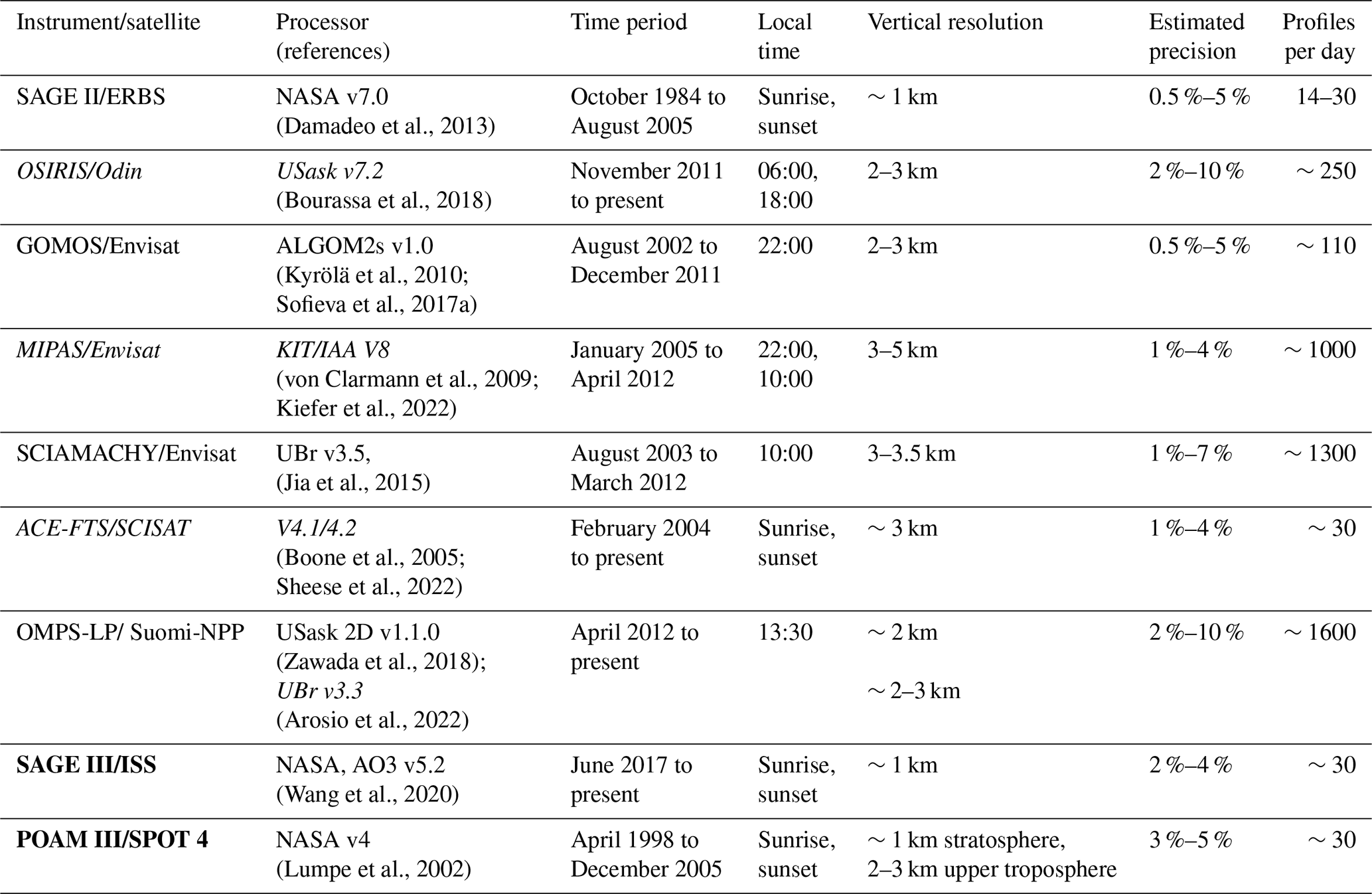
For creating the merged SAGE-CCI-OMPS+ dataset, we use the data from several limb and occultation instruments for which ozone profiles are retrieved on a geometric altitude grid. In the merged dataset, ozone profiles are also presented on an altitude grid from 10 to 50 km. The ozone profiles from individual instruments have a vertical resolution of 1–3 km in the stratosphere and in the UTLS (upper troposphere and lower stratosphere). The information about individual datasets is collected in Table 1. The majority of the datasets – SAGE II, SAGE III, POAM III, GOMOS, OSIRIS, SCIAMACHY, and OMPS – provide number density ozone profiles; therefore, this representation is adopted for the merged dataset. For ACE-FTS and MIPAS, the retrievals are in a volume mixing ratio on an altitude grid. Conversion to number density profiles is performed using temperature profiles retrieved by these instruments, as was done for SAGE-CCI-OMPS.
Table 1Information about the datasets used in the SAGE-CCI-OMPS+ dataset. Italic font indicates new versions of the datasets, and bold font indicates the new datasets used (compared to the SAGE-CCI-OMPS dataset).
For all instruments, we used ozone profile datasets from the user-friendly HARMonized dataset of OZone profiles (HARMOZ; Sofieva et al., 2013) developed in the Ozone_cci project. HARMOZ consists of the original retrieved ozone profiles from each instrument, which are screened for invalid data and presented on a common vertical grid and in a common netCDF4 format. In this work, we used altitude-gridded datasets (HARMOZ_ALT), available at https://climate.esa.int/en/projects/ozone/data/ (last access: 9 March 2023) and ftp://cci_web@ftp-ae.oma.be/esacci (last access: 9 March 2023).
Four datasets (GOMOS, SCIAMACHY, SAGE II, and OMPS-LP processed by the University of Saskatchewan) are the same as those used in SAGE-CCI-OMPS dataset (Sofieva et al., 2017b). Detailed information about these datasets can be found in Sofieva et al. (2013, 2017b). Below, we present the information about the new versions of the datasets (MIPAS, OSIRIS, and ACE-FTS) and new datasets (SAGE III/ISS, POAM III, and OMPS-LP processed by the University of Bremen) used in SAGE-CCI-OMPS+.
2.2 ACE-FTS v4
The ACE-FTS instrument (Bernath et al., 2005) flies on board the Canadian SCISAT satellite, which was launched in 2003 into a non-sun-synchronous, high-inclination orbit. The spectrometer is characterized by a high spectral resolution (0.02 cm−1) and views the Earth's limb in the infrared spectral range between 750 and 4400 cm−1. From its measurements, it is possible to derive volume mixing ratio (VMR) profiles of over 40 atmospheric trace gases and more than 20 isotopologue species, together with pressure and temperature information. ACE-FTS observes the atmospheric limb in the solar occultation mode between 5 and 150 km, with a vertical sampling of ∼2 to 6 km, depending on the orbital geometry and tangent height.
Recently, an improved retrieval version of the dataset has been released, and the ozone profiles have been validated against several independent observations (Sheese et al., 2022). The most recent retrieval algorithm is described in Boone et al. (2020), where the authors compare it to the previous v3.6 product. Version 4.1 has seen an update in spectroscopic information, including a new instrumental line shape, which improved the accuracy of forward-model calculations. In addition, a 100 m sub-grid was introduced within each 1 km layer of the vertical grid. To reduce systematic errors found in previous processing versions, changes were introduced in the handling of solar and deep-space calibration spectra.
Sheese et al. (2022) showed that the bias of v4.1 ozone data with respect to independent datasets is more stable with time in comparison to the previous version; i.e., the drift affecting the v3.6 data is substantially reduced in v4.1. In the lower stratosphere, v4.1 data have a bias of the order of −1 % to +5 %, with a drift within ±1 % per decade. In the middle stratosphere, a positive bias of 2 % to 9 % was found, although the time series has very good stability, with a drift within ±0.5 % per decade. Finally, in the upper stratosphere, v4.1 ozone shows a positive bias that increases with altitude (up to ∼15 %), with a drift within ±1 % per decade. Estimates indicate that the current product has a precision of the order of 0.1–0.2 ppmv (parts per million by volume) below 20 km and above 45 km (∼ 5 %–10 %, depending on altitude). Between 20 and 45 km, the estimated random uncertainty is ∼ 1 %–4 %.
2.3 MIPAS KIT v8
In the MIPAS IMK/IAA (a collaboration between the Karlsruhe Institute of Technology's Institute of Meteorology and Climate Research and the Instituto de Astrofísica de Andalucía) ozone retrievals, the v8 Level 1b dataset, with an improved characterization of detector aging (improved detector nonlinearity correction; see Sect. 5.6 in Kleinert et al., 2018), is used. This leads to less instrument-caused drift in the retrieved ozone values. In addition, the v8 temperature retrieval is improved due to use of better a priori information (Kiefer et al., 2021). The temperature retrieval results are used in the ozone retrieval. These improvements are relevant, especially for the upper stratosphere and mesosphere. In addition, ozone retrievals include the 3D structure of temperature retrieved in a previous step; thus, errors due to horizontal inhomogeneities are reduced (Kiefer et al., 2023).
Comparisons with ACE-FTS, MLS (Microwave Limb Sounder), and ozonesonde show approximately the same quality of v8 ozone as for v7. It is expected that the long-term stability of v8 is better than v7, particularly in the upper stratosphere.
2.4 OSIRIS v7.2
OSIRIS measurements are used to produce three long-term data records, namely vertically resolved profiles of ozone, nitrogen dioxide, and sulfate aerosols in the stratosphere and upper troposphere; recently, these processing chains have been merged, resulting in data product version 7.2 for each of the three species. Details related to the sulfate aerosol processing and the nitrogen dioxide processing can be found in Rieger et al. (2019) and Dubé et al. (2022), respectively. As the OSIRIS ozone retrieval is now coupled to the retrievals of these related species, they have a small impact on the OSIRIS ozone data record (Bognar et al., 2022). This work by Bognar et al. (2022) also details the changes between the previous version (V5.10) and version 7.2 of the OSIRIS ozone time series.
Although the impact was minor, within the version 7.2 update, many small changes were introduced to the OSIRIS data processing. The multiplicative algebraic reconstruction technique (MART; Degenstein et al., 2009) has been replaced by a Levenberg–Marquardt scheme. The OSIRIS pointing correction (Bourassa et al., 2018), developed specifically for the retrieval of ozone, has been implemented for all species (nitrogen dioxide and sulfate aerosols), further minimizing the impact on ozone of errors in these related species retrievals. The temperature-dependent OSIRIS spectral response function in the 320 nm region of the measured spectra has been diagnosed, and a correction has been implemented (see Appendix A in Bognar et al., 2022). The standard OSIRIS processing now uses temperature and pressure fields from the Modern-Era Retrospective analysis for Research and Applications version 2 (MERRA-2), as described in Wargan et al. (2017) and Gelaro et al. (2017). The BDM ozone absorption cross section, named for the authors of Brion et al. (1993), Daumont et al. (1992), and Malicet et al. (1995), has been implemented as part of the ozone retrieval. The lower bound of the OSIRIS ozone retrievals has been better defined through use of a new cloud detection scheme implemented for the OSIRIS aerosol product and described by Rieger et al. (2019). For more complete documentation of the OSIRIS version 7.2 ozone data product, please refer to https://arg.usask.ca/docs/osiris_v7/index.html (last access: 9 March 2023).
2.5 OMPS-LP ozone profiles processed by the University of Bremen
To retrieve the vertical distribution of ozone in the stratosphere from OMPS-LP observations, the radiative transfer model SCIATRAN is used, with a Tikhonov regularization approach to constrain the profile. Four spectral segments are selected, with three in the UV region and one in the Chappuis band. The altitude range over which the retrieval is performed spans between 8 and 60 km above sea level. Limb radiance in each spectral interval is first normalized with respect to a limb measurement at an upper tangent height. Simultaneously with the ozone retrieval, a surface reflectance estimation is performed exploiting the sun-normalized radiance at 38–40 km in the 340–345 and 675 nm ranges, respectively. Beforehand, a cloud filter is applied, and the retrieval of aerosol extinction profiles is performed. In addition, a retrieval of polar mesospheric cloud (PMC) properties is implemented, and this information is used in the ozone retrieval in the presence of PMCs. This improves the coverage of the dataset in polar regions during local summer. For a detailed description of the retrieval scheme, see Arosio et al. (2018). In the same paper, validation activities are also described, which mainly include comparisons with collocated ozonesondes and MLS observations. The discrepancies with respect to MLS profiles are well within ±10 % between 20 and 58 km at all latitudes, whereas the disagreement increases in the tropical UTLS. Ozonesondes are used to validate these OMPS-LP data in the lower stratosphere, and the best agreement was found at northern midlatitudes, with differences within ±3 % between 12 and 28 km. In the tropics, differences of about 8 %–12 % are found between 15 and 19 km. In the Southern Hemisphere, the comparison is not as good as in the Northern Hemisphere but still within ±7 % below 30 km.
The typical vertical resolution of the retrieved profiles is about 2–3 km, with larger values in the 30–35 km range, below 20 km in the tropics, and above 50 km at all latitudes. A thorough uncertainty analysis was performed and presented in Arosio et al. (2022). The typical retrieval noise spans 2 %–3 % between 15 and 50 km. The total random uncertainty is estimated in the range 3 %–5 % in the middle stratosphere, increasing in the UTLS. The total systematic uncertainty is mainly related to cloud contamination and model errors in the lower stratosphere and to the retrieval bias at high altitudes, with total values exceeding 5 % only above 50 km and below 20 km.
2.6 SAGE III/ISS v5.2
The second instrument of the SAGE III project (Chu and Veiga, 1998) was launched to the ISS in February 2017 and began routine operations in June 2017 that continue to the present. In a mid-inclination (∼52∘), low-Earth orbit (∼420 km), SAGE III/ISS (Cisewski et al., 2014) uses the solar occultation technique (McCormick et al., 1979) to make vertical profile measurements of ozone, aerosol extinction, water vapor, and nitrogen dioxide that cover the ∼ 70∘ S–70∘ N range on a monthly basis. While the instrument also makes measurements using the techniques of lunar occultation and limb scattering, those data are not used here. A detailed description of the solar occultation ozone retrieval can be found in Wang et al. (2020). Briefly, the AO3 ozone product that used here is derived from measurements in the Chappuis band (near 600 nm), together with aerosol measurements made in select channels across the visible and near-infrared range (∼ 520–1020 nm). This ozone product is reported from the surface or cloud top up to 70 km on a 0.5 km grid, with a vertical resolution of ∼ 1 km. The AO3 ozone product is preferred over the other stratospheric ozone product (i.e., multiple linear regression) because it has the best precision (∼ 2 %–4 %) and smallest differences compared to other satellites and ground stations (<5 % throughout the stratosphere (Wang et al., 2020). The version of data used here is v5.2, which is produced by NASA and is available at https://eosweb.larc.nasa.gov/project/SAGE III-ISS (last access: 9 March 2023), but it is also routinely transformed to the HARMOZ data format in the CCI project.
2.7 POAM III on SPOT 4
POAM III is a solar occultation instrument on the SPOT 4 satellite, which operated from 1998 to 2005. It flew in a sun-synchronous polar orbit, performing solar occultation observations in nine channels, covering the spectral range from 354 to 1018 nm. Successive measurements cover a fairly constant latitude band (55–71∘ N for sunrise; 63–88∘ S for sunset).
The altitude range for the NASA v4 retrieved ozone profiles spans the 5–60 km range, with a vertical resolution of 1 km in the stratosphere and 2–5 km in the upper troposphere. Typical retrieval uncertainties are reported to be within 5 % in the stratosphere, increasing up to 15 %–30 % in the troposphere. Aerosol extinction and sunspots are known to affect the retrievals from POAM III observations, mainly in the 20–40 km altitude range, which results in random errors of more than about 10 % in the stratosphere. However, according to Lumpe et al. (2002), less than 10 % of the ozone profiles are reported to suffer from sunspot-related artifacts.
The POAM III ozone product was validated against SAGE II, Halogen Occultation Experiment (HALOE), and balloon-borne observations, as described in Lumpe et al. (2002) and Randall et al. (2003). Results showed an agreement within 5 % in the 13–50 km range, whereas a 15 %–20 % high bias was found at lower altitudes.
2.8 Other datasets
In various data intercomparisons, we also used MLS v4.2 ozone profiles (MLS data were also transformed to the HARMOZ format), in addition to HEGIFTOM and SHADOZ ozonesonde profiles (available at https://hegiftom.meteo.be/datasets/ozonesondes, last access: 9 March 2023, and https://tropo.gsfc.nasa.gov/shadoz/Archive.html, last access: 9 March 2023; Witte et al., 2017; Thompson et al., 2017; Witte et al., 2018; Sterling et al., 2018; Van Malderen et al., 2016). For comparison with OMPS-LP data, ozonesonde profiles were collocated with the satellite observations, and the OMPS-LP averaging kernels were applied to degrade the high vertical resolution of sondes.
In this section, we present a short description of the merging method for the SAGE-CCI-OMPS dataset and its modification for SAGE-CCI-OMPS+. We also present detailed comparisons of deseasonalized anomalies for the new datasets included in SAGE-CCI-OMPS+.
3.1 A short description of the merging algorithm for the SAGE-CCI-OMPS dataset
A detailed description of the merging algorithm used for the SAGE-CCI-OMPS dataset is presented in Sofieva et al. (2017b). Here we present only a short description of this algorithm.
For the merged dataset, first the monthly zonal mean ozone profiles in 10∘ latitude bands from individual instruments are computed. Then, for each instrument, the deseasonalized anomalies are computed as follows:
where ρ(ti) is the monthly zonal mean number density value at a certain altitude and latitude band corresponding to time ti, and ρm is the mean over the whole considered time period for the corresponding month m for this altitude and latitude. For GOMOS, MIPAS, SCIAMACHY, ACE-FTS, and OSIRIS, the seasonal cycle is evaluated using the overlapping period 2005–2011. The seasonal cycle for SAGE II is computed using the years 1985–2004 and for OMPS using the years 2012–2020. Relative representation of the deseasonalized anomalies is chosen for visualization convenience.
The merging is performed as follows. In the first step, the median of GOMOS, MIPAS, SCIAMACHY, ACE-FTS, and OSIRIS deseasonalized anomalies is computed (pre-merging). In the second step, SAGE II deseasonalized anomalies are offset to the pre-merged anomalies in the years 2002–2005. The OMPS deseasonalized anomalies are offset to pre-merged anomalies (which are based on OSIRIS and ACE-FTS measurements in this period) in the years 2012–2020. After offsetting, all deseasonalized anomalies are aligned, and the median of deseasonalized anomalies from all instruments is computed. In the merging, we also applied a method for detection of outliers. We filtered out individual anomaly values (locally for each latitude band and altitude level), which differ from the median anomaly more than 10 % at latitudes 40∘ S–40∘ N and more than 20 % in other latitude bands. These thresholds are rather loose and do not affect the merged ozone in the overwhelming majority of cases; it removes only a few exceptional anomalies, which appear in rare cases for instruments with rather coarse sampling (such as GOMOS and ACE-FTS).
The merged deseasonalized anomalies can be used directly to estimate ozone trends. For other applications, the merged ozone number density profiles are also provided. The computation of the number density profiles from the merged deseasonalized anomalies is performed via restoring the seasonal cycle according to Eq. (1). For the SAGE-CCI-OMPS, the amplitude of the seasonal cycle is estimated using MIPAS measurements because they provide all season pole-to-pole measurements with dense sampling. The absolute values of the seasonal cycle are estimated from SAGE II and OSIRIS in the overlapping period (which are very close to each other and to GOMOS measurements), thus preserving the consistency in the dataset through the whole observation period.
3.2 Comparisons of the new datasets
Different intercomparisons of the new datasets have been performed. In this section, we show some illustrations and discuss the impacts of using new datasets in the merging.
On the monthly zonal mean level, MIPAS v8 ozone profiles are 1 %–2 % larger than those of v7 in the middle stratosphere and ∼1 % smaller at ∼45 km, as illustrated in Fig. 1. This decrease at ∼45 km seems to be related to a change in the retrieval vertical grid width at this altitude in v7, while the v8 processor uses the grid with a constant spacing up to 55 km. In the mesosphere, v8 reports 2 %–6 % smaller values over the tropics and middle latitudes. In the polar winter stratosphere, MIPAS v8 has 2 %–7 % larger values compared to v7 data. The differences in the UTLS are of larger magnitude ( %), and they change from altitude to altitude (Fig. 1). Figure 2 shows the difference in the deseasonalized anomalies (defined by Eq. 1). As illustrated in Fig. 2, the deseasonalized anomalies computed from MIPAS v8 and v7 data are very similar (typical patterns of the anomalies themselves can be seen in Fig. 12; they are in the range of %).
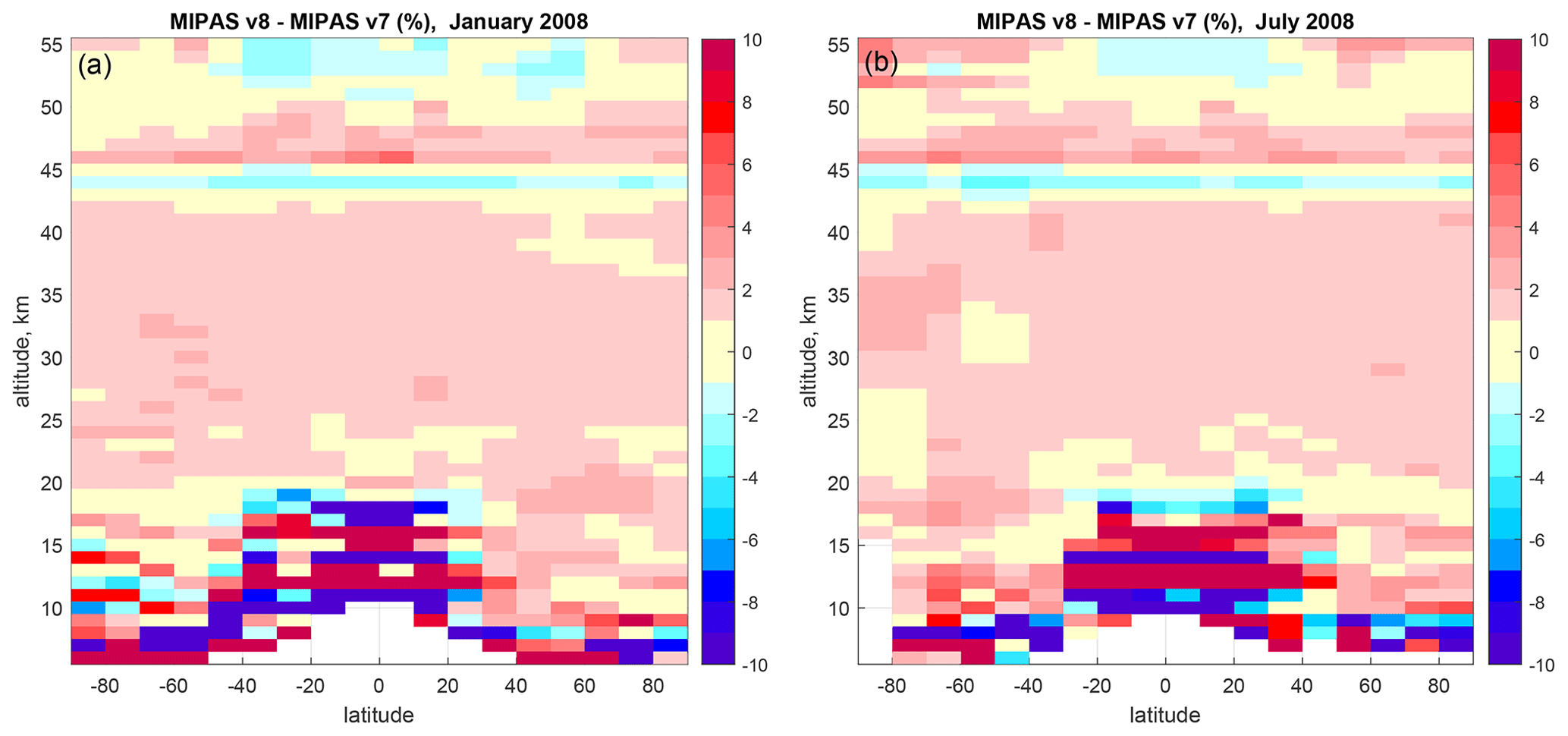
Figure 1Relative difference in MIPAS v8 and v7 monthly zonal mean ozone profiles for January 2008 (a) and July 2008 (b). The altitude range below 55 km is shown.
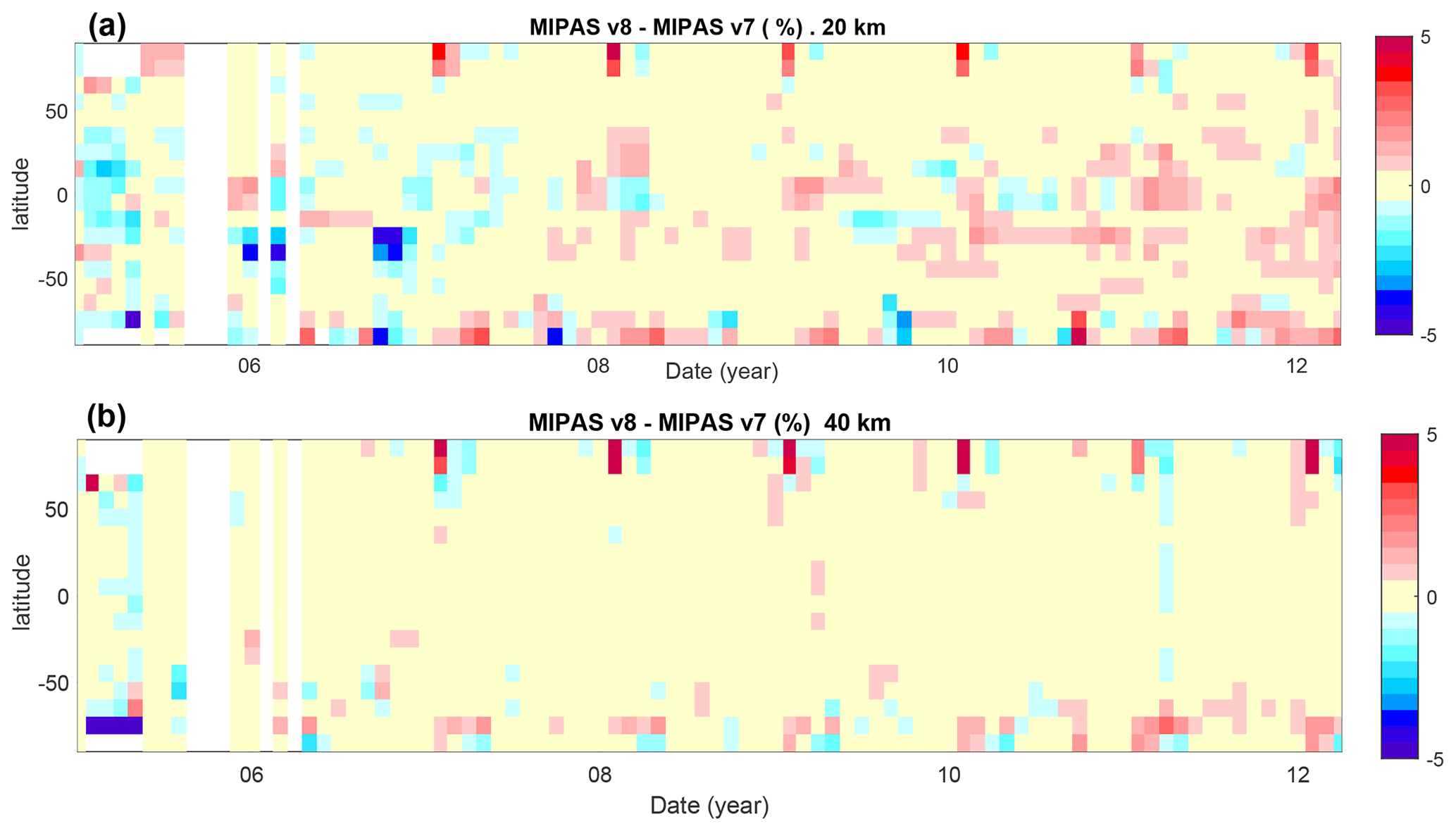
Figure 2Difference in the deseasonalized anomalies between MIPAS v8 and v7 ozone data (v8 minus v7; in %), for altitudes at 20 km (a) and 40 km (b).
ACE-FTS v4.1/4.2 monthly zonal mean ozone profiles are 2 %–4 % larger than those of v3.5/3.6 in the middle stratosphere and ∼ 1 %–4 % smaller at altitudes 50–55 km, as illustrated by Fig. 3. The differences in the UTLS are ± 4 %–8 %; their sign and magnitude are altitude and latitude dependent. ACE-FTS v4.1/4.2 ozone data have a smaller drift. This is illustrated in Fig. 4, which compares differences to MLS deseasonalized anomalies at 40 km for ACE-FTS v3.5/3.6 ozone profiles (Fig. 3a) and ACE-FTS v4.1/4.2 data (Fig. 3b). The progressing differences (drift) of v3.5/3.6 with respect to MLS largely disappears for v4.1/4.2. This deviation of ACE-FTS v3.5/3.6 with respect to MLS anomalies increases with altitude between 10 and 50 km (not shown). The analogous behavior is also observed in comparison with the merged SAGE-CCI-OMPS deseasonalized anomalies (Fig. S1 in the Supplement), but the difference is slightly less visible because ACE-FTS data are used in construction of a SAGE-CCI-OMPS merged dataset. A small positive deviation of ACE-FTS v4.1/4.2 relative to MLS anomalies starting in 2019 can be observed in Fig. 4.
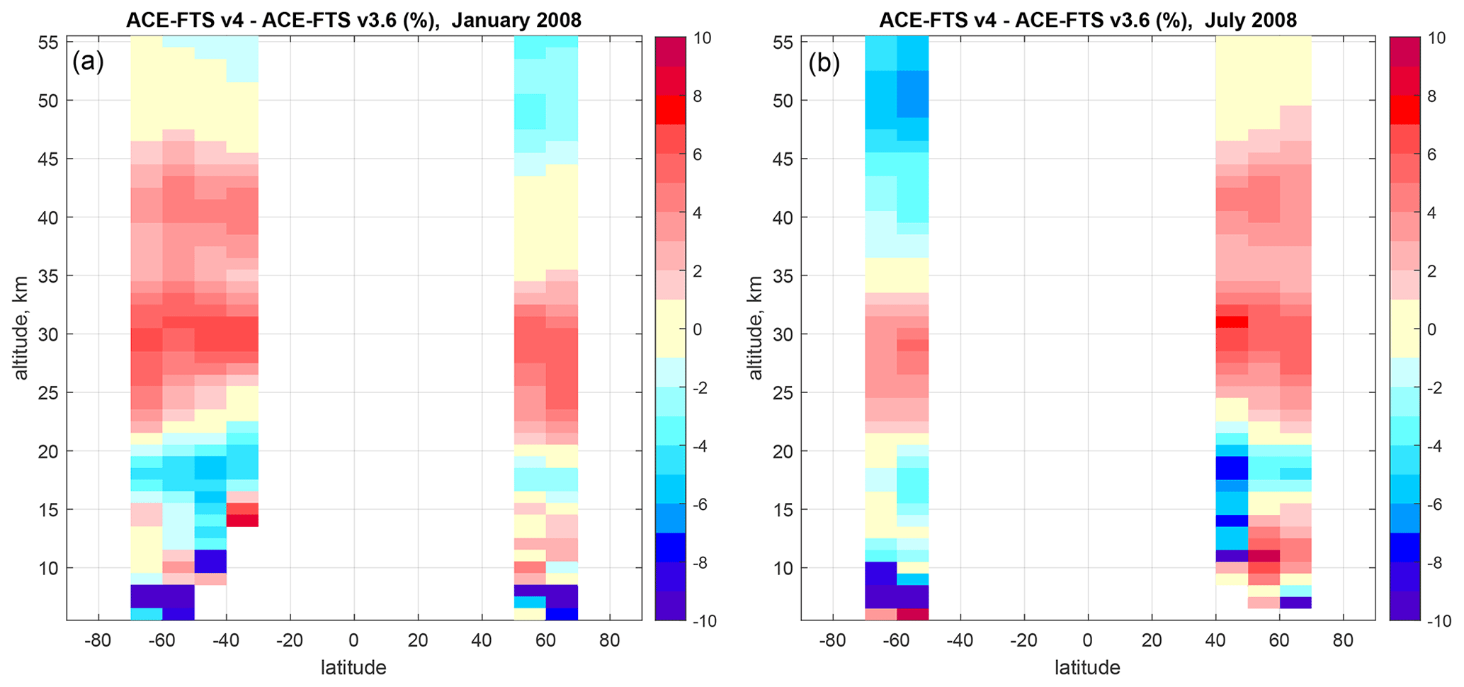
Figure 3Relative difference in ACE-FTS v4.1/4.2 and v3.5/3.6 monthly zonal mean ozone profiles for January 2008 (a) and July 2008 (b). The altitude range below 55 km is shown.
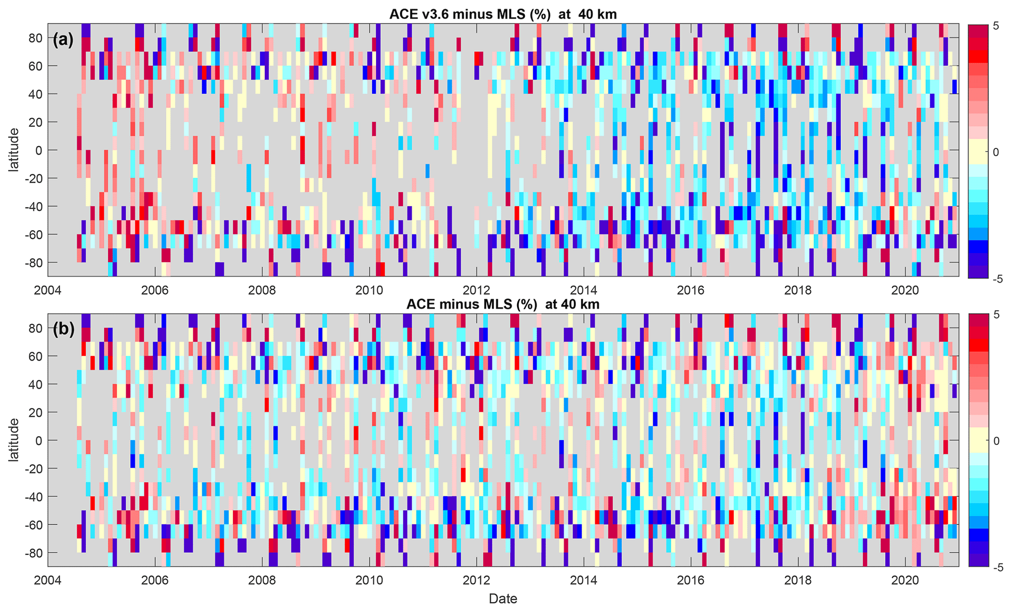
Figure 4Difference in deseasonalized anomalies for ACE-FTS minus MLS (in %) at 40 km for ACE-FTS v3.5/3.6 (a) and v4.1/4.2 (b).
OSIRIS v7.2 ozone profiles cover a larger altitude range compared to the OSIRIS v5.10 data. This can be seen by comparing Fig. 5a and b. OSIRIS v7.2 monthly zonal mean ozone profiles are 1 %–5 % smaller in the middle stratosphere, mostly ∼ 2 %–7 % larger in the lower stratosphere, and more than 10 % smaller in the troposphere compared to the analogous monthly zonal mean ozone profiles evaluated using OSIRIS v5.10 data. The difference, with respect to the analogous MLS deseasonalized anomalies, is slightly different between OSIRIS v5.10 and OSIRIS v7.2 because the latter anomalies are closer to those of MLS before 2006 but larger in 2014–2016, as shown in Fig. 6.
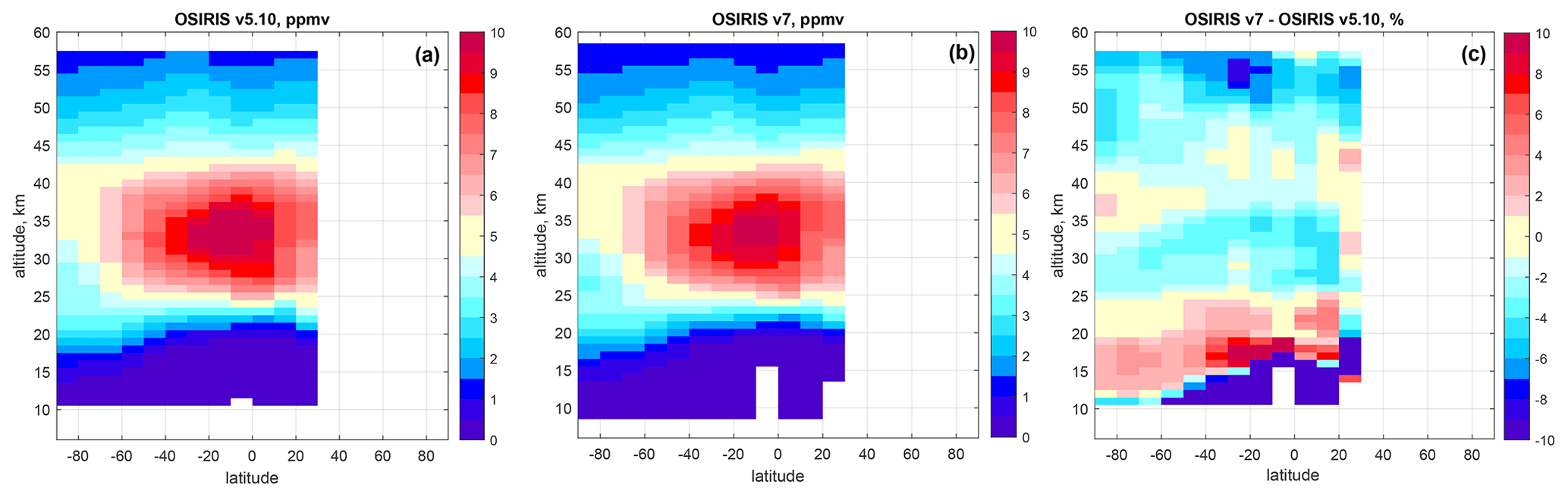
Figure 5Monthly zonal mean ozone profiles in January 2008 evaluated using OSIRIS v5.10 data (a) and v7 data (b). (c) Relative difference in OSIRIS v7 and v5.10 monthly zonal mean ozone profiles for January 2008.
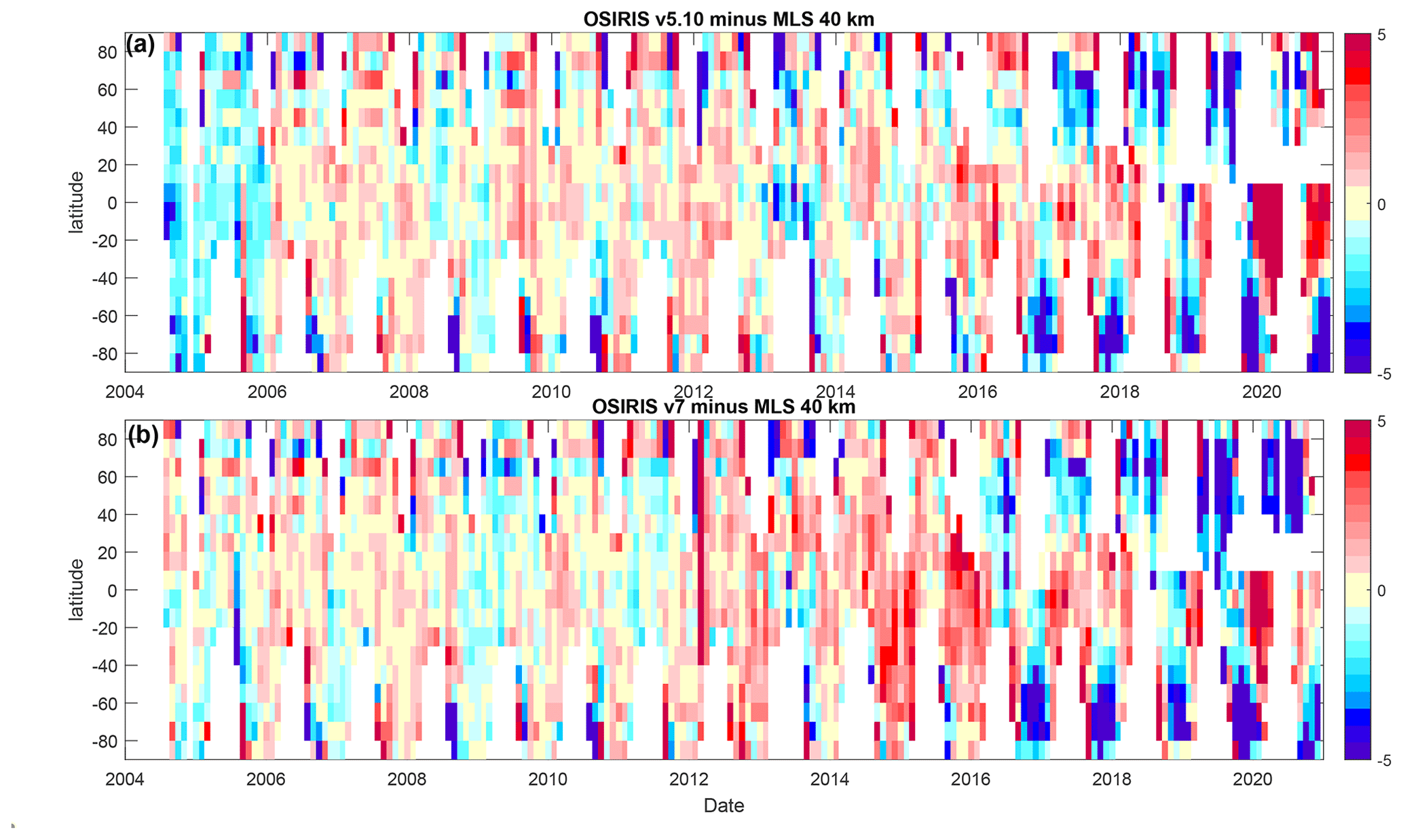
Figure 6Difference in deseasonalized ozone anomalies (in %) between OSIRIS and MLS at 40 km for OSIRIS v5.10 (a) and v7 (b).
The OMPS-LP ozone profiles processed by the University of Bremen (UBr) and the University of Saskatchewan (USask) have a slightly different vertical extent (larger for OMPS UBr), as illustrated in Fig. 7a and b. Due to different thresholds on the solar zenith angle, polar regions are better covered by OMPS USask data (Fig. 7a, b). The biases of monthly zonal mean data can be up to 10 % in the middle stratosphere and even larger near the tropical tropopause (Fig. 7c). Despite the difference in absolute ozone values, the deseasonalized anomalies from OMPS UBr and USask data are very similar in majority of cases, as illustrated in Fig. 8, which suggests that the idea of using the mean of UBr and USask deseasonalized anomalies as the OMPS anomalies might be viable. The averaging can be done by ignoring missing data (i.e., if data are missing in one of the datasets, then they will follow the existing data from another dataset). The intercomparison of OMPS and UBr ozone deseasonalized anomalies is aimed at assessing whether the averaging of deseasonalized anomalies is advantageous and at defining a valid range of OMPS data. For this, the OMPS UBr and USask deseasonalized anomalies are compared with deseasonalized anomalies from MLS and from the merged SAGE-CCI-OMPS dataset.
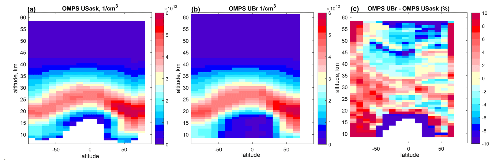
Figure 7Monthly zonal mean ozone profiles in January 2018 evaluated using OMPS-LP USask data (a) and OMPS-LP UBr data (b). (c) Relative difference in OMPS UBr and OMPS USask monthly zonal mean ozone profiles for January 2018.
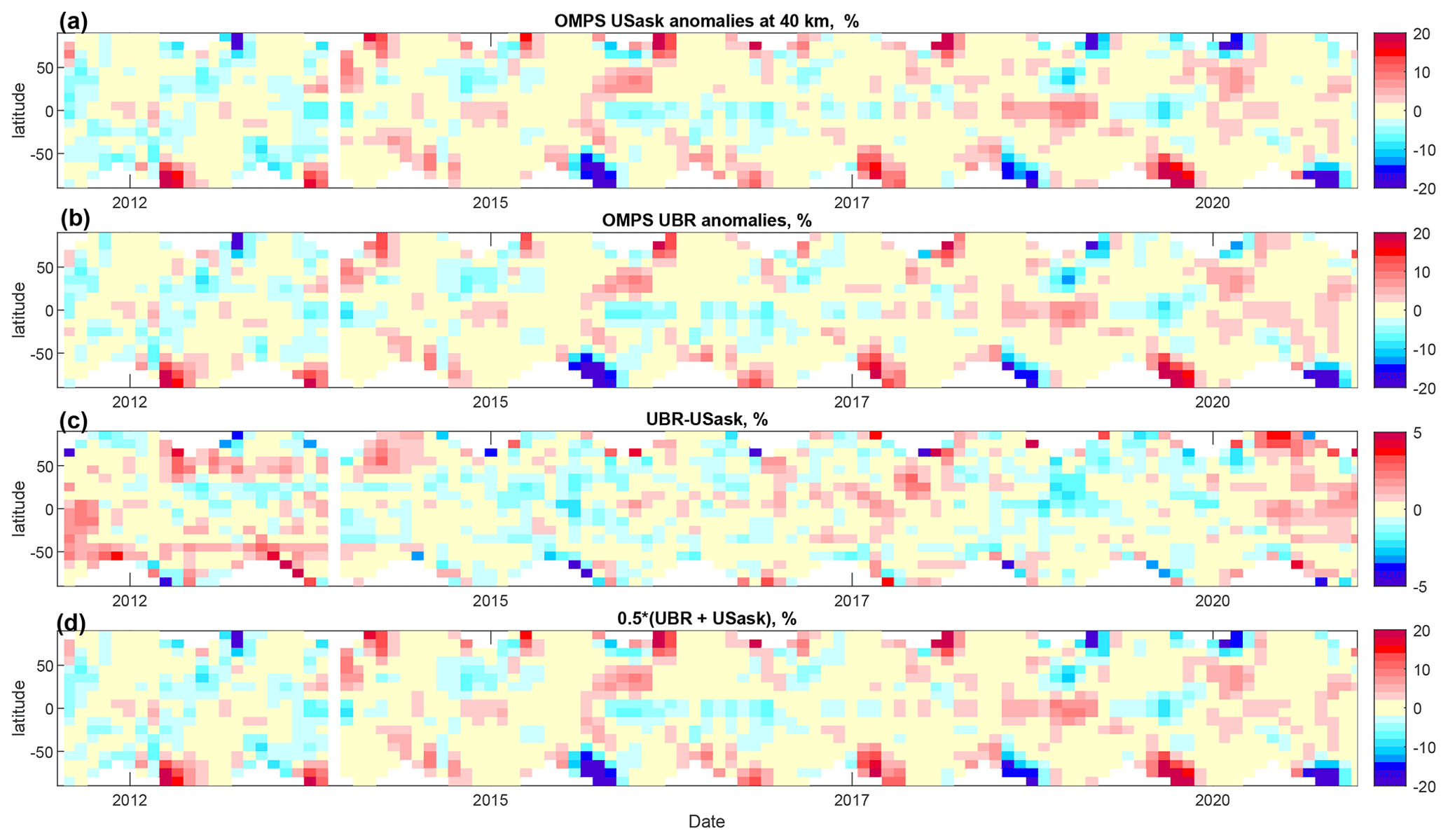
Figure 8(a) OMPS USask and (b) OMPS UBr deseasonalized ozone anomalies at 40 km, (c) difference between OMPS UBr and USask deseasonalized ozone anomalies at 40 km, and (d) mean of OMPS UBr and USask deseasonalized ozone anomalies at 40 km.
In polar regions, USask data have better coverage, as illustrated in Fig. 9, which compares the deseasonalized anomalies from UBr (Fig. 9a), USask (Fig. 9b), and MLS (Fig. 9d) for 70–80∘ N. Using OMPS-LP USask data in cases when UBr data are missing is advantageous from the point of view of data coverage. In these cases, the OMPS USask anomalies are close to those of MLS in the majority of cases. Here we would like to note that the data with strongly inhomogeneous spatial or temporal sampling are not used in the deseasonalized anomalies (see also Sect. 3.3). There are also periods in which OMPS USask data have pronounced deviations from MLS anomalies, such as in winters with large anomaly values (e.g., in Northern Hemisphere winter 2016 and 2018; see also Fig. S2), while these periods are not covered by UBr data. At lower altitudes, the mean of OMPS UBr and USask anomalies are closer to MLS anomalies, compared to each dataset separately, as observed in Fig. S2. Such behavior – smaller deviations of the mean of the OMPS UBr and USask deseasonalized anomalies from MLS or from merged SAGE-CCI-anomalies – are also observed for other latitude bands, as illustrated in Fig. 10. This indicates that averaging of OMPS UBr and USask deseasonalized anomalies is advantageous.
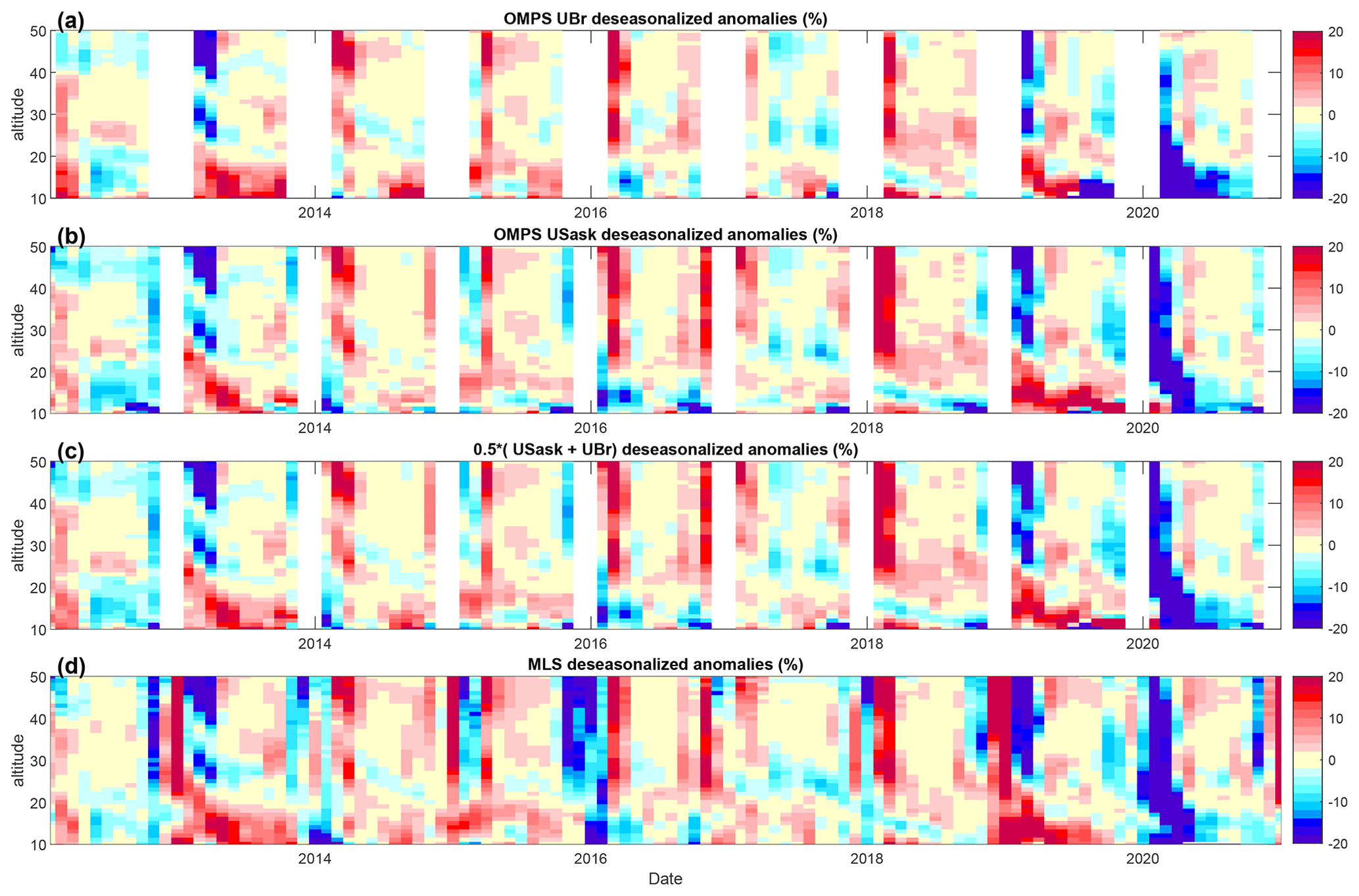
Figure 9Deseasonalized anomalies at 70–80∘ N for (a) OMPS UBr ozone data, (b) OMPS USask ozone data, (c) mean of USask and UBr deseasonalized anomalies (ignoring missing data), and (d) MLS deseasonalized anomalies.
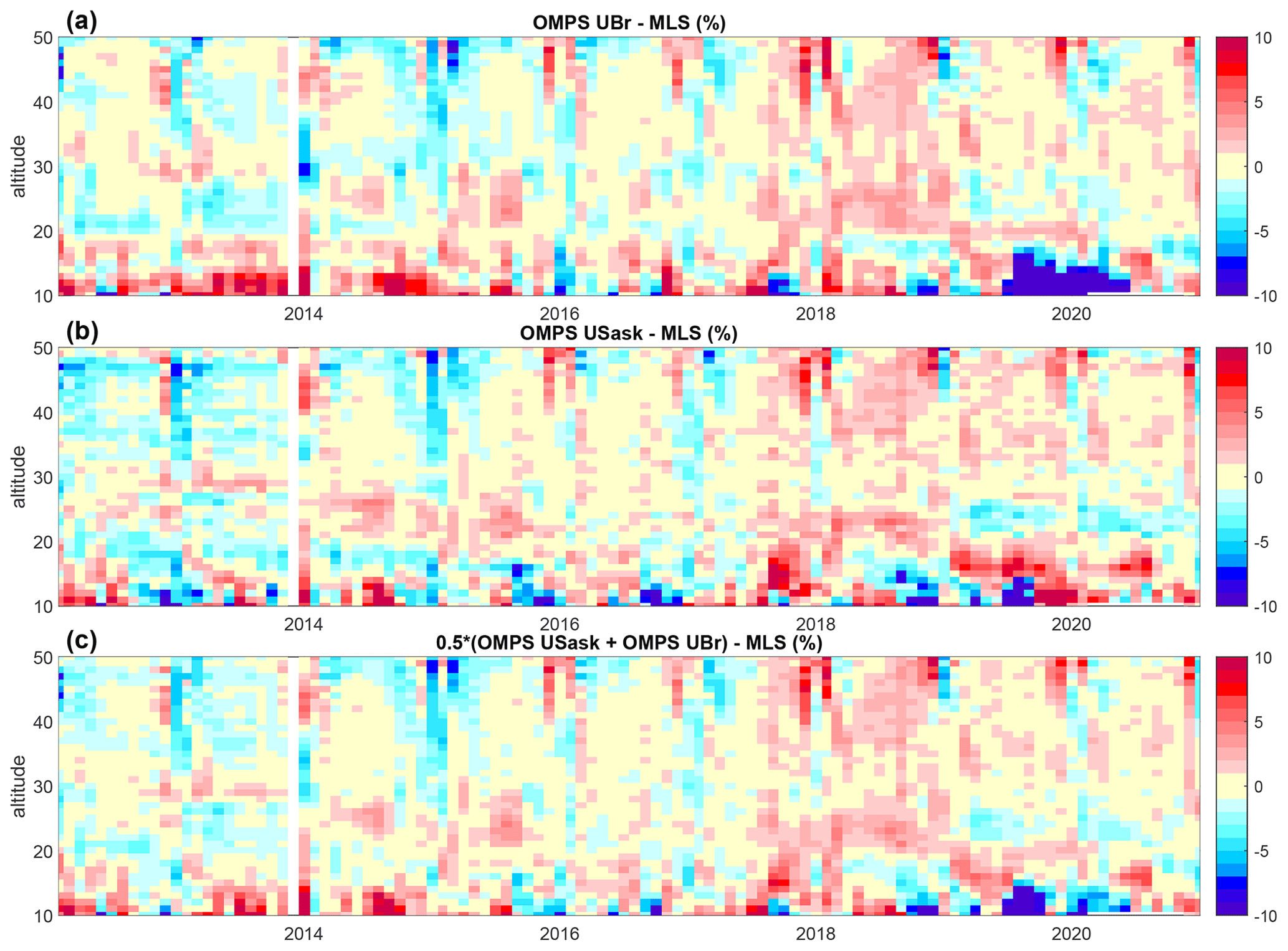
Figure 10Difference between OMPS and MLS deseasonalized anomalies at 50–60∘ N for (a) OMPS UBr, (b) OMPS USask, and (c) mean of OMPS UBr and USask datasets.
In the tropical upper troposphere at 14–16 km, we found a strong drift (or a step) in OMPS UBr data, which was observed in comparison with the MLS, merged SAGE-CCI-OMPS dataset, and ozonesondes (illustrations can be found in the Supplement; see Figs. S3–S6). At other altitudes in the tropical troposphere and UTLS, OMPS-LP UBr data show reasonable agreement with ozonesondes and MLS data. At altitudes 10–13 km, ozone variations and differences between different data are large, as illustrated in Fig. S4, but the drift is strongly reduced, as can be seen in Fig. S5. Comparing sondes, MLS, and OMPS UBr at 15.5 km (Fig. S6), we notice that the negative drift at this altitude with respect to MLS is enhanced by the positive drift of MLS with respect to sondes.
POAM III data mainly cover the polar regions in 1998–2005, while SAGE III/ISS data are mostly within the ∼ 60∘ S–60∘ N latitude range (Fig. 11). As observed from Fig. 11, which shows the difference in POAM III and SAGE III/ISS deseasonalized anomalies with respect to the merged SAGE-CCI-OMPS anomalies, the anomalies are in rather good agreement with the merged SAGE-CCI-OMPS dataset at a majority of altitudes. One can notice a larger deviation of SAGE III/ISS from the baseline SAGE-CCI–OMPS anomalies at 20 km in the tropics over the first year of SAGE III/ISS data (Fig. 11). In comparison with MLS, however, the same deviation in SAGE III/ISS data is only noticeable between December 2017 and January 2018, albeit with a smaller magnitude (Fig. S7). At the moment, the SAGE III/ISS observational period is too short to make conclusions about the systematic nature of the deviations.
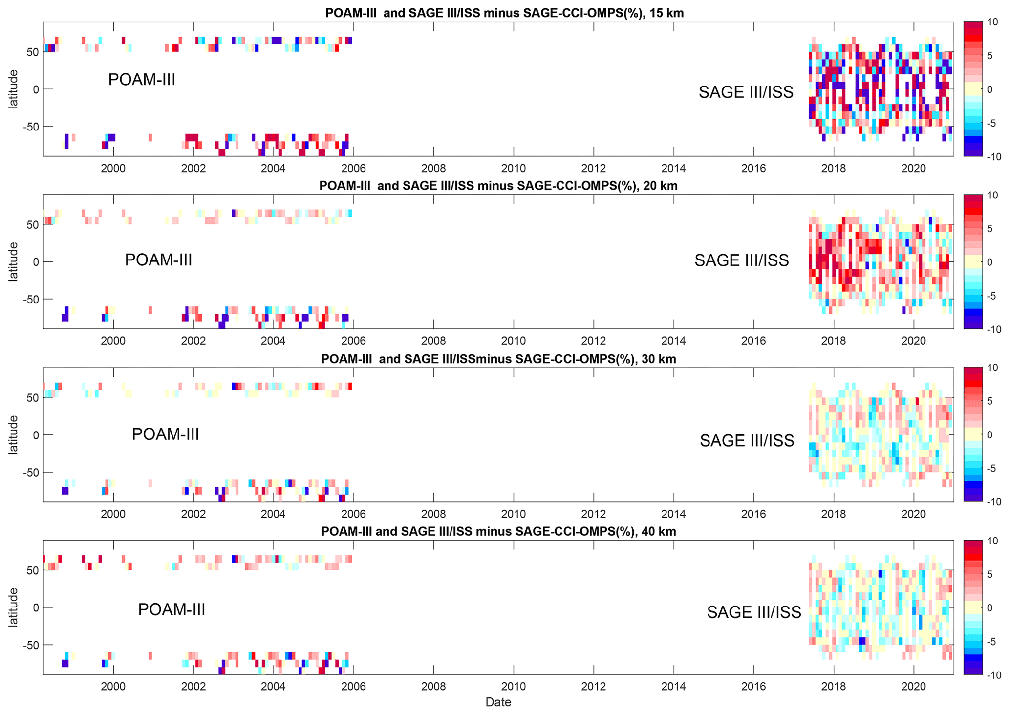
Figure 11Difference in POAM III and SAGE III/ISS deseasonalized ozone anomalies with respect to SAGE-CCI-OMPS at several altitude levels.
3.3 Data merging in the SAGE-CCI-OMPS+ dataset
The merging procedure of SAGE-CCI-OMPS+ dataset is very similar to that for SAGE-CCI-OMPS dataset; it is based on using the deseasonalized anomalies. Compared to SAGE-CCI-OMPS dataset, we improved the data filtering from latitude-time bins with highly inhomogeneous sampling. Now they are ignored if the inhomogeneity measure in either latitude Hlat or in time Htime exceeds 0.9 (in the original dataset, the filtering criterion was ). The definitions of the inhomogeneity measure is presented in Sofieva et al. (2017b, 2014). This filtering only removes a few data points corresponding to highly inhomogeneous sampling, which are mostly for occultation instruments and for data in polar regions.
Similar to the SAGE-CCI-OMPS dataset, we use only single-instrument data that do not exhibit significant drift with respect to collocated, ground-based observations and with respect to each other. For this reason, we do not to use the SCIAMACHY data before August 2003, OMPS data before April 2012, GOMOS data after November 2011, and MIPAS data in 2002–2004 in the merged dataset (the illustrations and discussions of these data exclusions are presented in Sofieva et al., 2017b). In SAGE-CCI-OMPS+, we excluded OMPS UBr data at altitudes 14–16 km in the tropical region 20∘ S–20∘ N. We use the mean of OMPS USask and UBr deseasonalized anomalies (ignoring missing values) as the contribution from OMPS in the merged dataset.
Using the same technique as for the SAGE-CCI-OMPS dataset, we first perform pre-merging via the computation of the median GOMOS, MIPAS, SCIAMACHY, ACE-FTS, and OSIRIS deseasonalized anomalies. Then SAGE II, OMPS, POAM III, and SAGE III/ISS deseasonalized anomalies are offset to the pre-merged anomalies using the corresponding overlapping periods. After that, the outlier detection and the final merging (computing the median of all aligned deseasonalized anomalies) is performed. As an example, Fig. 12 shows deseasonalized anomalies from individual instruments and merged anomalies at 30 km.
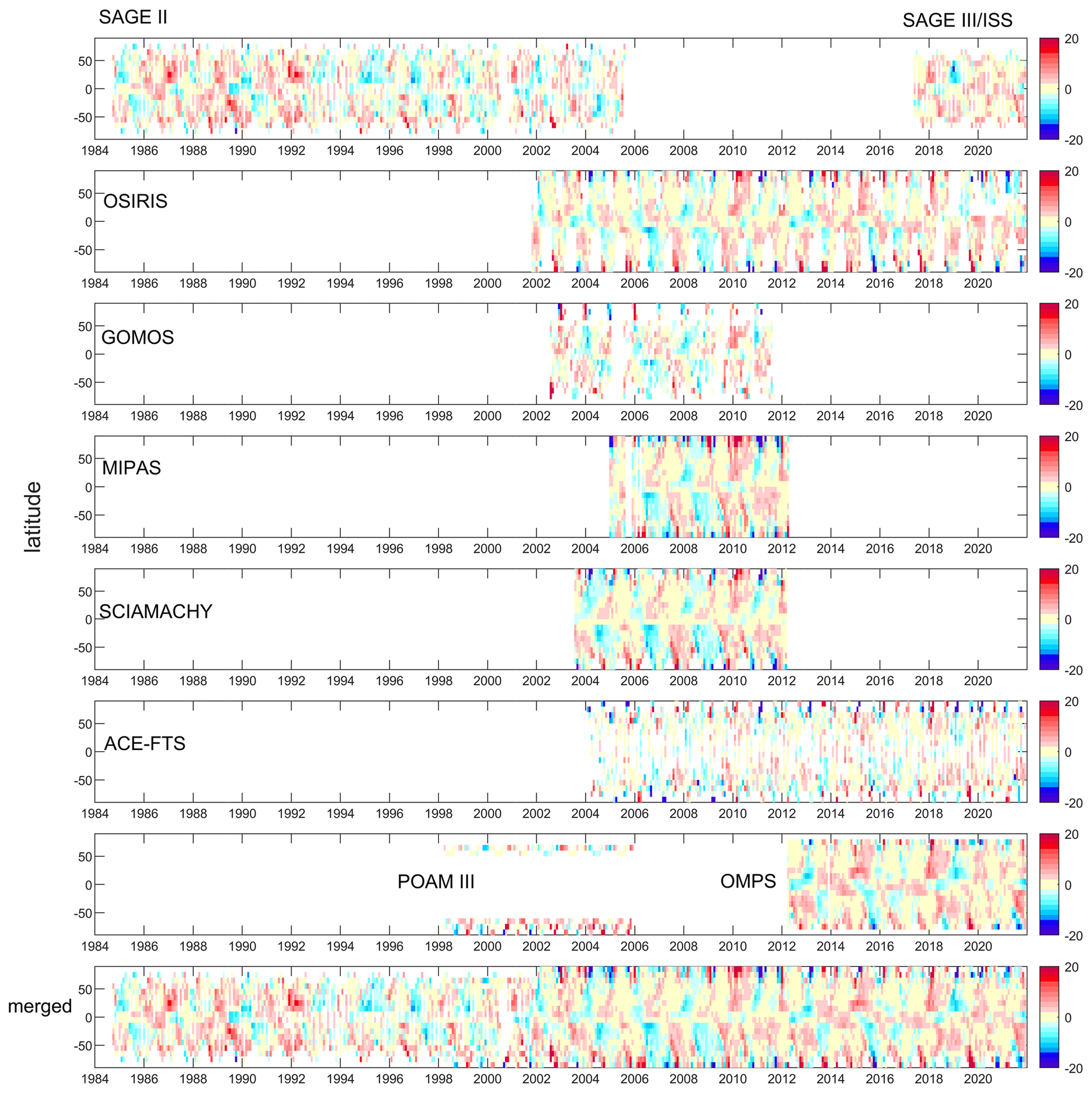
Figure 12Deseasonalized ozone anomalies from individual datasets and the merged time series (SAGE-CCI-OMPS+) at 30 km.
The procedure of the reconstruction of ozone concentrations from the merged deseasonalized anomalies is the same as for the SAGE-CCI-OMPS dataset. It is described in Sect. 3.1; the illustration of the seasonal cycle in individual ozone datasets can be found in the Supplement (Fig. S14). Some illustrations of SAGE-CCI-OMPS and SAGE-CCI-OMPS+ datasets are shown in Fig. 13, which compares the ozone time series at 30 km and ozone profile time series close to the Equator (0–10∘ N). As shown in Fig. 13a and c, the SAGE-CCI-OMPS+ dataset has a better coverage of polar regions due to inclusion of POAM III data. The SAGE-CCI-OMPS+ dataset also has a better coverage of the UTLS region (Fig. 13b, d) due to inclusion of SAGE III and OMPS-LP UBr data.
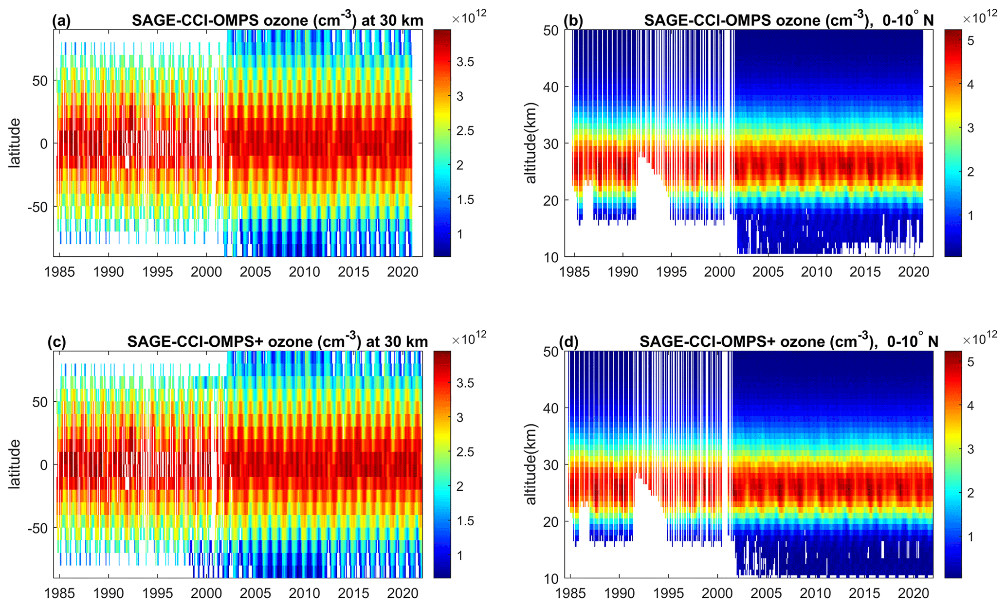
Figure 13Time series of ozone at 30 km in the merged SAGE-CCI-OMPS (a) and SAGE-CCI-OMPS+ (c) datasets. Time series of ozone profiles at 0–10∘ N in SAGE-CCI-OMPS (b) and SAGE-CCI-OMPS+ (d).
The estimation of uncertainties in the SAGE-CCI-OMPS+ dataset is performed in the same way as for the original version (Sofieva et al., 2017b), where uncertainties in the monthly zonal mean data from individual instruments are propagated through all steps of the merging procedure. The uncertainty in the merged ozone anomalies is defined as follows (Sofieva et al., 2017b):
where is the anomaly uncertainty in the instrument corresponding to the median value. Thus, the uncertainty in merged anomalies depends on the agreement of deseasonalized anomalies used for the computation of the median values. It is smaller than if several instruments report a similar anomaly. Figure 14 illustrates the mean uncertainties in the original and updated SAGE-CCI-OMPS deseasonalized ozone anomalies in two periods (2005–2010 and 2015–2020). Before 2002, the uncertainties remain nearly the same as in the original SAGE-CCI-OMPS dataset because this period is covered mainly by the SAGE II data. In the stratosphere, estimated uncertainties are very close for both SAGE-CCI-OMPS and SAGE-CCI-OMPS+ datasets. In the tropical UTLS, the estimated uncertainties in the SAGE-CCI-OMPS+ dataset are ∼ 0.5 %–1.5 % larger in 2005–2010 (compared to SAGE-CCI-OMPS), mostly due to larger variations in OSIRIS v7 ozone anomalies. On the contrary, a pronounced reduction in estimated uncertainties in 2015–2020 (by more than 2 %) is found in 2015–2020, which is mainly related to the use of additional datasets (SAGE III/ISS and OMPS UBr) and the overall improved agreement between individual datasets.
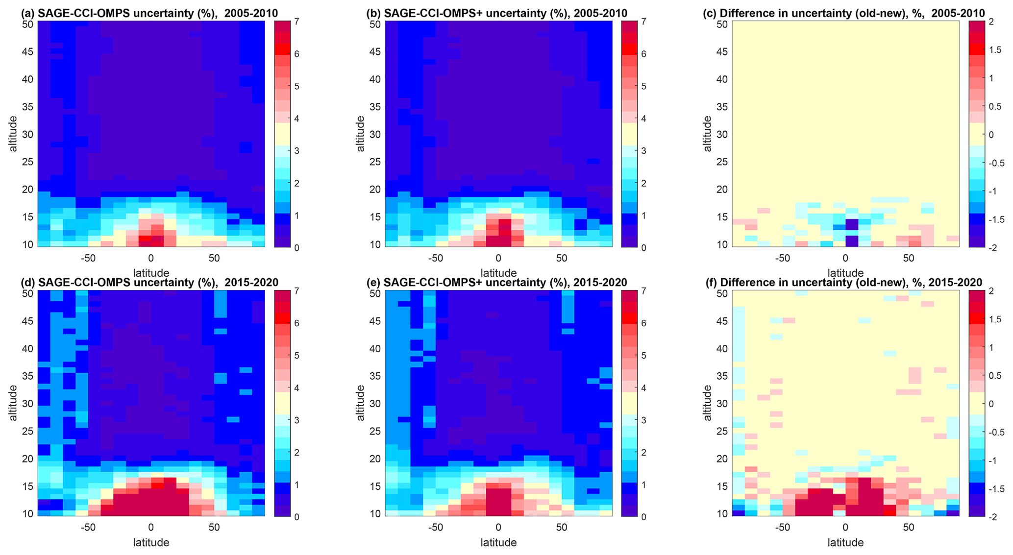
Figure 14SAGE-CCI-OMPS uncertainties in merged ozone in (a) 2005–2010 and (d) 2015–2020. SAGE-CCI-OMPS+ uncertainties in (b) 2005–2010 and (e) 2015–2020. Difference in uncertainties (%) between SAGE-CCI-OMPS and SAGE-CCI-OMPS+ in (c) 2005–2010 and (f) 2015–2020.
The objective of the analysis presented in this section is the investigation of sensitivity of ozone trends to the changes in the datasets used for data merging. For this, we created a series of test datasets in which only one change was introduced. For example, MIPAS v7 was replaced by MIPAS v8 or ACE-FTS v3.5/3.6 was replaced by ACE-FTS v4.1/4.2, and we added SAGE III, while other datasets are as in the original SAGE-CCI-OMPS dataset, and so on.
For studies of trends sensitivity, we used a simple regression model, as follows:
where PWLT(t, t0) is a piecewise linear term (constant and a hockey-stick trend with the turnaround point in 1997), QBO30(t) and QBO50(t) are the equatorial winds at 30 and 50 hPa, respectively (https://www.cpc.ncep.noaa.gov/data/indices/, last access: 9 March 2023), F10.7(t) is the monthly average solar 10.7 cm radio flux (https://www.spaceweather.gc.ca/forecast-prevision/solar-solaire/solarflux/sx-en.php, last access: 9 March 2023; https://psl.noaa.gov/data/correlation/solar.data, last access: 9 March 2023), and ENSO(t) is the 2-month lagged El Niño–Southern Oscillation (ENSO) proxy (https://psl.noaa.gov/enso/mei/, last access: 9 March 2023).
Although the regression model is rather simple, it was used in previous trend analyses (Kyrölä et al., 2013; Sofieva et al., 2017b, 2021). It was shown in Petropavlovskikh et al. (2019) that the evaluated trends weakly depend on the regression model. We would like to add a caveat that the trend estimates in polar regions are less accurate, due to the large year-to-year variability and absence of dynamical proxies (which can partly explain this variability) in the regression model.
Figures 15 and S8–S13 show the differences in the trend estimates caused by changes in the dataset. The figures in the Supplement show the trends for the baseline SAGE-CCI-OMPS dataset (left panels), trends when the corresponding change in one dataset was introduced (central panels), and the difference (new minus baseline), which are shown in right panels of Figs. S8–S13 and also in Fig. 15. All these figures show post-1997 trends corresponding to the second part of the piecewise linear fit by Eq. (3).
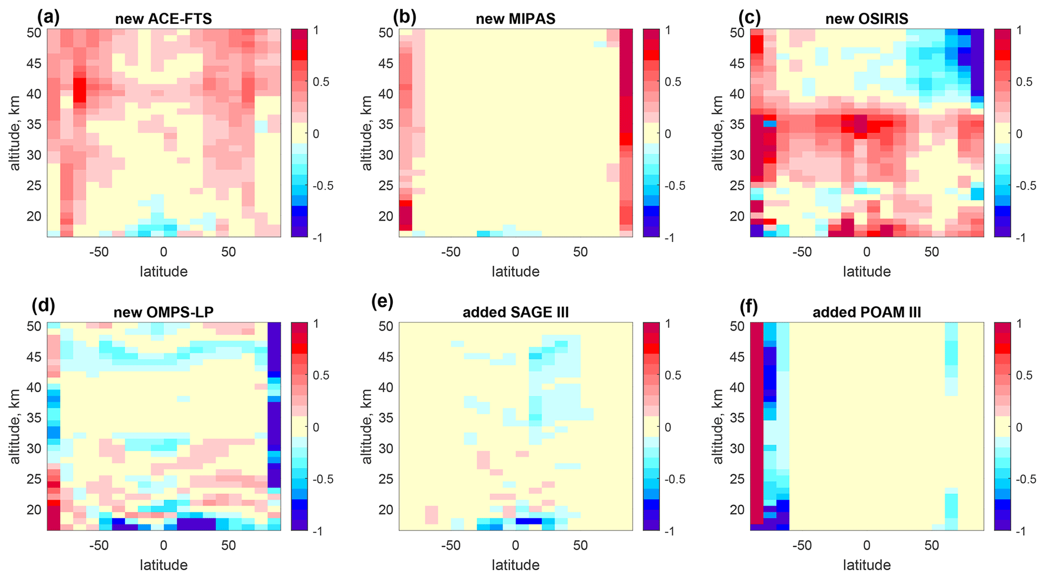
Figure 15Difference in trends estimated (in % per decade), as caused by changes in the datasets (new minus baseline; see the text for an explanation).
Using ACE-FTS v4.1/4.2 instead of ACE-FTS v3.5/3.6 results in ∼ 0.5 % per decade to 0.7 % per decade larger ozone trends in the upper stratosphere, as shown in Figs. 15a and S8 (consistent with the analysis presented in Sect. 3.2). Using MIPAS v8 instead of MIPAS v7 affects the trend estimates only at high latitudes (Figs. 15b and S9), where the estimated trends become ∼1 % per decade larger. Using the new OSIRIS ozone dataset v7 affects the trends at all altitudes and all latitudes so that ozone trends become ∼ 0.5 % per decade to 1 % per decade larger in the middle stratosphere but ∼ 0.5 % per decade to 1 % per decade smaller in the northern upper stratosphere (Figs. 15c and S10). Using both OMPS USask and UBr datasets has a rather small impact on evaluated ozone trends; some visible reductions in the trends occur in the tropical upper troposphere and close to North Pole (Figs. 15d and S11). Adding SAGE III data has a small impact on ozone trends (Figs. 15e and S12). This is expected, as SAGE III deseasonalized anomalies agree very well with the merged SAGE-CCI-OMPS dataset, and the SAGE III time series is relatively short (Sect. 3.2). Adding ozone profiles from POAM III results in a slight decrease in ozone trends at 60–80∘ S (by ∼ 0.3 % per decade to 1 % per decade) and a pronounced increase in ozone trends of more than 1 % per decade near the South Pole (Figs. 15f and S13).
Overall, using new datasets has a rather small impact on the resulting trends at latitudes 60∘ S–60∘ N (typically within ±0.5 % per decade). The effect is more pronounced in polar regions, which is rather expected due to scarcer data coverage, and significantly larger ozone variability (note the caveats on the regression model mentioned above).
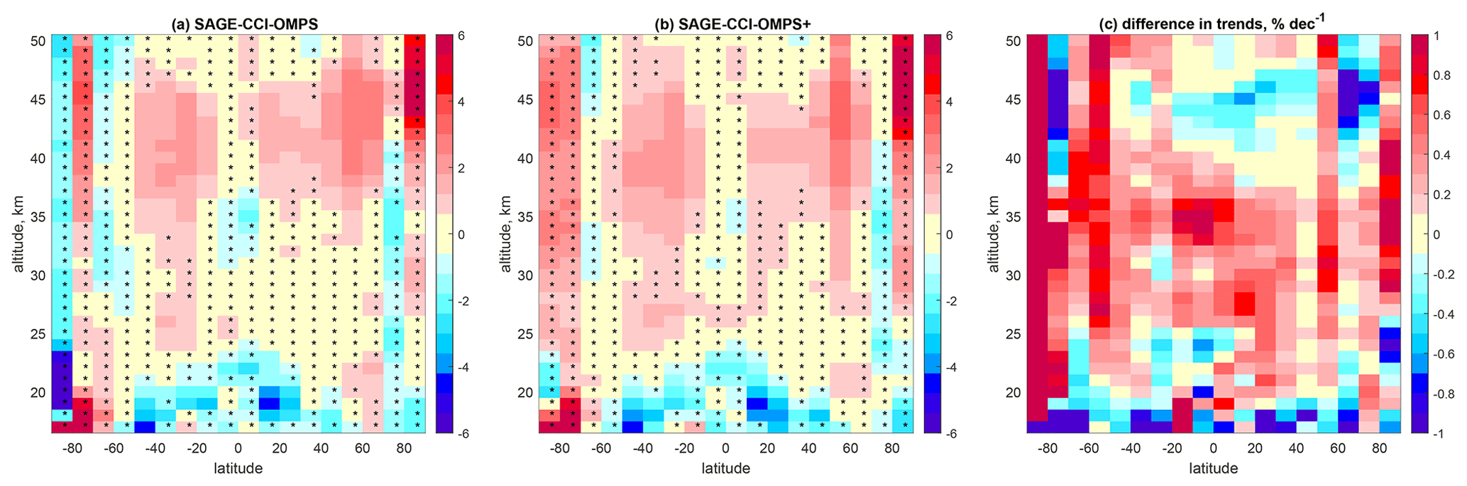
Figure 16Ozone trends in 1997–2020 (% per decade) evaluated using the baseline SAGE-CCI-OMPS dataset (a) and the SAGE-CCI-OMPS+ dataset (b). Stars indicate the latitude–altitude bins in which trends are not statistically significant at the 95 % confidence level. Panel (c) shows the difference in ozone trends (in % per decade; new minus baseline).
Post-1997 ozone trends evaluated using SAGE-CCI-OMPS and SAGE-CCI-OMPS+ datasets (the regression analysis has been done using the common period 1984–2020) are shown in Fig. 16. The overall structure of ozone trends is very similar in both merged datasets because the trends in the upper stratosphere are positive and statistically significant. There are a few altitude–latitude bins in which negative trends in the lower stratosphere are statistically significant, and they are similar in old and new merged datasets. The largest changes are at highest latitudes (80–90∘, especially in the Southern Hemisphere). At other latitude bands, the influence on ozone trends is rather small (usually less than 0.5 % per decade).
SAGE-CCI-OMPS+ is an updated version of the SAGE-CCI-OMPS merged dataset. In addition to the ozone profiles from SAGE II, OSIRIS, GOMOS, MIPAS, SCIAMACHY, ACE-FTS, and OMPS-LP used in the original dataset, SAGE-CCI-OMPS+ also includes the ozone profile datasets from POAM III and SAGE III/ISS. For MIPAS, ACE-FTS, and OSIRIS, the ozone data from updated processors are used. In the updated dataset, both OMPS-LP ozone profiles processed by University of Saskatchewan and University of Bremen are used, and taking the mean of deseasonalized anomalies as an OMPS-LP dataset improves the spatial coverage and agreement with other datasets. We performed a detailed intercomparison of datasets from individual instruments. The new processed ozone datasets from ACE-FTS, MIPAS, and OSIRIS are expected to be more stable.
The merging method is similar to that used for creating the SAGE-CCI-OMPS dataset. It is based on the median of aligned deseasonalized anomalies from individual instruments. The updated SAGE-CCI-OMPS+ has a better coverage of polar regions and the UTLS.
We analyzed the sensitivity of ozone trends, which are estimated using multiple linear regression, to the inclusion of new datasets. Overall, the changes in ozone trends are within ±0.5 % per decade in the majority of latitude bins and altitudes, and they do not change the overall morphology of the trends in ozone profiles; statistically significant trends are observed in the upper stratosphere.
The updated SAGE-CCI-OMPS+ dataset covers the period from October 1984 to December 2021, and it will be regularly extended in the future. The profiles of ozone concentrations and deseasonalized anomalies are provided on an altitude grid from 10 to 50 km and in 10∘ latitude bins from 90∘ S to 90∘ N. The SAGE-CCI-OMPS+ dataset can be used for the evaluation of ozone trends in the stratosphere and other research.
The open-access CCI datasets are available from the ESA Climate Office at https://climate.esa.int/en/projects/ozone/data/ (ftp://cci_web@ftp-ae.oma.be/esacci, last access: 9 March 2023). The SAGE-CCI-OMPS dataset is also available through the Climate Data Store (CDS) of the Copernicus Climate Change Service (C3S) (2020; https://doi.org/10.24381/cds.4ebfe4eb).
The supplement related to this article is available online at: https://doi.org/10.5194/amt-16-1881-2023-supplement.
VFS designed the study, performed the analyses, and wrote the majority of the paper. MS participated in the trend analyses. RD, CA, AR, MS, JT, MW, DD, AB, DZ, MK, AL, KAW, PS, DH, MvR, CR, and JDL provided the data and contributed to the analyses and writing of the paper.
At least one of the (co-)authors is a member of the editorial board of Atmospheric Measurement Techniques. The peer-review process was guided by an independent editor, and the authors also have no other competing interests to declare.
Publisher’s note: Copernicus Publications remains neutral with regard to jurisdictional claims in published maps and institutional affiliations.
This article is part of the special issue “Atmospheric ozone and related species in the early 2020s: latest results and trends (ACP/AMT inter-journal SI)”. It is not associated with a conference.
The work was performed in the framework of the ESA Ozone_cci+ project (contract no. 4000126562/19/I-NB). The KIT team would like to thank the European Space Agency (ESA) for providing access to MIPAS Level 1 data. The ozone retrieval from SCIAMACHY and OMPS-LP instruments at the University of Bremen was funded in part by ESA (including the Living Planet Fellowship SOLVE), German Aerospace Agency (DLR), German Research Foundation (DFG), through the research unit VolImpact (grant no. FOR2820), the University of Bremen, and the state of Bremen. The dataset was calculated with resources provided by the North German Supercomputing Alliance (HLRN). The GALAHAD Fortran Library was employed in the retrieval scheme. The GOMOS ALGOM2s dataset was created in the framework of the ESA ALGOM project. Processing of MIPAS data used in this study was partly funded by DLR (contract no. 50EE1547; SEREMISA). The MIPAS dataset computations were performed in the frame of a Bundesprojekt (grant no. MIPAS_V7) on the Cray XC40 “Hazel Hen” of the High-Performance Computing Center Stuttgart (HLRS) of the University of Stuttgart. The FMI team thanks the Academy of Finland (Centre of Excellence of Inverse Modelling and Imaging; decision 336798). The ACE mission is supported primarily by the Canadian Space Agency (CSA). Odin is a Swedish-led satellite project funded jointly by Sweden (SNSB), Canada (CSA), France (CNES), and Finland (Tekes). The authors thank Gabriele Stiller (KIT) for comments on this work.
This research has been supported by the European Space Agency (grant nos. 4000126562/19/I-NB and SOLVE), the Academy of Finland (Centre of Excellence of Inverse Modelling and Imaging; decision 336798), and the Deutsches Zentrum für Luft- und Raumfahrt (DLR; SEREMISA; grant no. 50EE1547).
This paper was edited by Ja-Ho Koo and reviewed by three anonymous referees.
Arosio, C., Rozanov, A., Malinina, E., Eichmann, K.-U., von Clarmann, T., and Burrows, J. P.: Retrieval of ozone profiles from OMPS limb scattering observations, Atmos. Meas. Tech., 11, 2135–2149, https://doi.org/10.5194/amt-11-2135-2018, 2018.
Arosio, C., Rozanov, A., Gorshelev, V., Laeng, A., and Burrows, J. P.: Assessment of the error budget for stratospheric ozone profiles retrieved from OMPS limb scatter measurements, Atmos. Meas. Tech., 15, 5949–5967, https://doi.org/10.5194/amt-15-5949-2022, 2022.
Bernath, P. F., McElroy, C. T., Abrams, M. C., Boone, C. D., Butler, M., Camy-Peyret, C., Carleer, M., Clerbaux, C., Coheur, P.-F., Colin, R., DeCola, P., DeMazière, M., Drummond, J. R., Dufour, D., Evans, W. F. J., Fast, H., Fussen, D., Gilbert, K., Jennings, D. E., Llewellyn, E. J., Lowe, R. P., Mahieu, E., McConnell, J. C., McHugh, M., McLeod, S. D., Michaud, R., Midwinter, C., Nassar, R., Nichitiu, F., Nowlan, C., Rinsland, C. P., Rochon, Y. J., Rowlands, N., Semeniuk, K., Simon, P., Skelton, R., Sloan, J. J., Soucy, M.-A., Strong, K., Tremblay, P., Turnbull, D., Walker, K. A., Walkty, I., Wardle, D. A., Wehrle, V., Zander, R., and Zou, J.: Atmospheric Chemistry Experiment (ACE): Mission overview, Geophys. Res. Lett., 32, L15S01, https://doi.org/10.1029/2005GL022386, 2005.
Bognar, K., Tegtmeier, S., Bourassa, A., Roth, C., Warnock, T., Zawada, D., and Degenstein, D.: Stratospheric ozone trends for 1984–2021 in the SAGE II–OSIRIS–SAGE III/ISS composite dataset, Atmos. Chem. Phys., 22, 9553–9569, https://doi.org/10.5194/acp-22-9553-2022, 2022.
Boone, C. D., Nassar, R., Walker, K. A., Rochon, Y., McLeod, S. D., Rinsland, C. P., and Bernath, P. F.: Retrievals for the atmospheric chemistry experiment Fourier-transform spectrometer, Appl. Optics, 44, 7218–7231, 2005.
Boone, C. D., Bernath, P. F., Cok, D., Jones, S. C., and Steffen, J.: Version 4 retrievals for the atmospheric chemistry experiment Fourier transform spectrometer (ACE-FTS) and imagers, J. Quant. Spectrosc. Ra., 247, 106939, https://doi.org/10.1016/j.jqsrt.2020.106939, 2020.
Bourassa, A. E., Roth, C. Z., Zawada, D. J., Rieger, L. A., McLinden, C. A., and Degenstein, D. A.: Drift-corrected Odin-OSIRIS ozone product: algorithm and updated stratospheric ozone trends, Atmos. Meas. Tech., 11, 489–498, https://doi.org/10.5194/amt-11-489-2018, 2018.
Brasseur, G. P. and Solomon, S.: Aeronomy of the Middle Atmosphere, 3rd edn., D. Reidel Publishing Company, ISBN-10 1402032846, 2005.
Brion, J., Chakir, A., Daumont, D., Malicet, J., and Parisse, C.: High-resolution laboratory absorption cross section of O3. Temperature effect, Chem. Phys. Lett., 213, 610–612, https://doi.org/10.1016/0009-2614(93)89169-I, 1993.
Chu, W. P. and Veiga, R.: SAGE III/EOS, in: Optical Remote Sensing of the Atmosphere and Clouds, SPIE, 52–60, https://doi.org/10.1117/12.577943, 1998.
Cisewski, M., Zawodny, J., Gasbarre, J., Eckman, R., Topiwala, N., Rodriguez-Alvarez, O., Cheek, D., and Hall, S.: The Stratospheric Aerosol and Gas Experiment (SAGE III) on the International Space Station (ISS) Mission, in: Sensors, Systems, and Next-Generation Satellites XVIII, SPIE, 924107, https://doi.org/10.1117/12.2073131, 2014.
Copernicus Climate Change Service (C3S) Climate Data Store (CDS) [data set]: Ozone monthly gridded data from 1970 to present derived from satellite observations, https://doi.org/10.24381/cds.4ebfe4eb, 2020.
Damadeo, R. P., Zawodny, J. M., Thomason, L. W., and Iyer, N.: SAGE version 7.0 algorithm: application to SAGE II, Atmos. Meas. Tech., 6, 3539–3561, https://doi.org/10.5194/amt-6-3539-2013, 2013.
Daumont, D., Brion, J., Charbonnier, J., and Malicet, J.: Ozone UV spectroscopy I: Absorption cross-sections at room temperature, J. Atmos. Chem., 15, 145–155, https://doi.org/10.1007/BF00053756, 1992.
Degenstein, D. A., Bourassa, A. E., Roth, C. Z., and Llewellyn, E. J.: Limb scatter ozone retrieval from 10 to 60 km using a multiplicative algebraic reconstruction technique, Atmos. Chem. Phys., 9, 6521–6529, https://doi.org/10.5194/acp-9-6521-2009, 2009.
Dubé, K., Zawada, D., Bourassa, A., Degenstein, D., Randel, W., Flittner, D., Sheese, P., and Walker, K.: An improved OSIRIS NO2 profile retrieval in the upper troposphere–lower stratosphere and intercomparison with ACE-FTS and SAGE III/ISS, Atmos. Meas. Tech., 15, 6163–6180, https://doi.org/10.5194/amt-15-6163-2022, 2022.
ESA Climate Office: Ozone data, ESA Climate Office [data set], https://climate.esa.int/en/projects/ozone/data/ (ftp://cci_web@ftp-ae.oma.be/esacci), last access: 9 March 2023.
Gelaro, R., McCarty, W., Suárez, M. J., Todling, R., Molod, A., Takacs, L., Randles, C. A., Darmenov, A., Bosilovich, M. G., Reichle, R., Wargan, K., Coy, L., Cullather, R., Draper, C., Akella, S., Buchard, V., Conaty, A., da Silva, A. M., Gu, W., Kim, G.-K., Koster, R., Lucchesi, R., Merkova, D., Nielsen, J. E., Partyka, G., Pawson, S., Putman, W., Rienecker, M., Schubert, S. D., Sienkiewicz, M., and Zhao, B.: The Modern-Era Retrospective Analysis for Research and Applications, Version 2 (MERRA-2), J. Climate, 30, 5419–5454, https://doi.org/10.1175/JCLI-D-16-0758.1, 2017.
Godin-Beekmann, S., Azouz, N., Sofieva, V. F., Hubert, D., Petropavlovskikh, I., Effertz, P., Ancellet, G., Degenstein, D. A., Zawada, D., Froidevaux, L., Frith, S., Wild, J., Davis, S., Steinbrecht, W., Leblanc, T., Querel, R., Tourpali, K., Damadeo, R., Maillard Barras, E., Stübi, R., Vigouroux, C., Arosio, C., Nedoluha, G., Boyd, I., Van Malderen, R., Mahieu, E., Smale, D., and Sussmann, R.: Updated trends of the stratospheric ozone vertical distribution in the 60∘ S–60∘ N latitude range based on the LOTUS regression model, Atmos. Chem. Phys., 22, 11657–11673, https://doi.org/10.5194/acp-22-11657-2022, 2022.
Jia, J., Rozanov, A., Ladstätter-Weißenmayer, A., and Burrows, J. P.: Global validation of SCIAMACHY limb ozone data (versions 2.9 and 3.0, IUP Bremen) using ozonesonde measurements, Atmos. Meas. Tech., 8, 3369–3383, https://doi.org/10.5194/amt-8-3369-2015, 2015.
Kiefer, M., von Clarmann, T., Funke, B., García-Comas, M., Glatthor, N., Grabowski, U., Kellmann, S., Kleinert, A., Laeng, A., Linden, A., López-Puertas, M., Marsh, D. R., and Stiller, G. P.: IMK/IAA MIPAS temperature retrieval version 8: nominal measurements, Atmos. Meas. Tech., 14, 4111–4138, https://doi.org/10.5194/amt-14-4111-2021, 2021.
Kiefer, M., von Clarmann, T., Funke, B., García-Comas, M., Glatthor, N., Grabowski, U., Höpfner, M., Kellmann, S., Laeng, A., Linden, A., López-Puertas, M., and Stiller, G. P.: Version 8 IMK–IAA MIPAS ozone profiles: nominal observation mode, Atmos. Meas. Tech., 16, 1443–1460, https://doi.org/10.5194/amt-16-1443-2023, 2023.
Kleinert, A., Birk, M., Perron, G., and Wagner, G.: Level 1b error budget for MIPAS on ENVISAT, Atmos. Meas. Tech., 11, 5657–5672, https://doi.org/10.5194/amt-11-5657-2018, 2018.
Kyrölä, E., Tamminen, J., Sofieva, V., Bertaux, J. L., Hauchecorne, A., Dalaudier, F., Fussen, D., Vanhellemont, F., Fanton d'Andon, O., Barrot, G., Guirlet, M., Mangin, A., Blanot, L., Fehr, T., Saavedra de Miguel, L., and Fraisse, R.: Retrieval of atmospheric parameters from GOMOS data, Atmos. Chem. Phys., 10, 11881–11903, https://doi.org/10.5194/acp-10-11881-2010, 2010.
Kyrölä, E., Laine, M., Sofieva, V., Tamminen, J., Päivärinta, S.-M., Tukiainen, S., Zawodny, J., and Thomason, L.: Combined SAGE II–GOMOS ozone profile data set for 1984–2011 and trend analysis of the vertical distribution of ozone, Atmos. Chem. Phys., 13, 10645–10658, https://doi.org/10.5194/acp-13-10645-2013, 2013.
Lumpe, J. D., Bevilacqua, R. M., Hoppel, K. W., and Randall, C. E.: POAM III retrieval algorithm and error analysis, J. Geophys. Res.-Atmos., 107, ACH 5-1–ACH 5-32, https://doi.org/10.1029/2002JD002137, 2002.
Malicet, J., Daumont, D., Charbonnier, J., Parisse, C., Chakir, A., and Brion, J.: Ozone UV Spectroscopy II: Absorption Cross-Sections and Temperature Dependence, J. Atmos. Chem., 21, 263–273, 1995.
McCormick, M. P., Hamill, P., Pepin, T. J., Chu, W. P., Swissler, T. J., and McMaster, L. R.: Satellite Studies of the Stratospheric Aerosol, B. Am. Meteorol. Soc., 60, 1038–1047, https://doi.org/10.1175/1520-0477(1979)060<1038:SSOTSA>2.0.CO;2, 1979.
Petropavlovskikh, I., Godin-Beekmann, S., Hubert, D., Damadeo, R., Hassler, B., and Sofieva, V.: SPARC/IO3C/GAW Report on Long-term Ozone Trends and Uncertainties in the Stratosphere, SPARC Report No. 9, GAW Report No. 241, https://doi.org/10.17874/f899e57a20b, 2019.
Randall, C. E., Rusch, D. W., Bevilacqua, R. M., Hoppel, K. W., Lumpe, J. D., Shettle, E., Thompson, E., Deaver, L., Zawodny, J., Kyrö, E., Johnson, B., Kelder, H., Dorokhov, V. M., König-Langlo, G., and Gil, M.: Validation of POAM III ozone: Comparisons with ozonesonde and satellite data, J. Geophys. Res.-Atmos., 108, 4367, https://doi.org/10.1029/2002JD002944, 2003.
Rieger, L. A., Zawada, D. J., Bourassa, A. E., and Degenstein, D. A.: A Multiwavelength Retrieval Approach for Improved OSIRIS Aerosol Extinction Retrievals, J. Geophys. Res.-Atmos., 124, 7286–7307, https://doi.org/10.1029/2018JD029897, 2019.
Sheese, P. E., Walker, K. A., Boone, C. D., Bourassa, A. E., Degenstein, D. A., Froidevaux, L., McElroy, C. T., Murtagh, D., Russell III, J. M., and Zou, J.: Assessment of the quality of ACE-FTS stratospheric ozone data, Atmos. Meas. Tech., 15, 1233–1249, https://doi.org/10.5194/amt-15-1233-2022, 2022.
Sofieva, V. F., Rahpoe, N., Tamminen, J., Kyrölä, E., Kalakoski, N., Weber, M., Rozanov, A., von Savigny, C., Laeng, A., von Clarmann, T., Stiller, G., Lossow, S., Degenstein, D., Bourassa, A., Adams, C., Roth, C., Lloyd, N., Bernath, P., Hargreaves, R. J., Urban, J., Murtagh, D., Hauchecorne, A., Dalaudier, F., van Roozendael, M., Kalb, N., and Zehner, C.: Harmonized dataset of ozone profiles from satellite limb and occultation measurements, Earth Syst. Sci. Data, 5, 349–363, https://doi.org/10.5194/essd-5-349-2013, 2013.
Sofieva, V. F., Kalakoski, N., Päivärinta, S.-M., Tamminen, J., Laine, M., and Froidevaux, L.: On sampling uncertainty of satellite ozone profile measurements, Atmos. Meas. Tech., 7, 1891–1900, https://doi.org/10.5194/amt-7-1891-2014, 2014.
Sofieva, V. F., Ialongo, I., Hakkarainen, J., Kyrölä, E., Tamminen, J., Laine, M., Hubert, D., Hauchecorne, A., Dalaudier, F., Bertaux, J.-L., Fussen, D., Blanot, L., Barrot, G., and Dehn, A.: Improved GOMOS/Envisat ozone retrievals in the upper troposphere and the lower stratosphere, Atmos. Meas. Tech., 10, 231–246, https://doi.org/10.5194/amt-10-231-2017, 2017a.
Sofieva, V. F., Kyrölä, E., Laine, M., Tamminen, J., Degenstein, D., Bourassa, A., Roth, C., Zawada, D., Weber, M., Rozanov, A., Rahpoe, N., Stiller, G., Laeng, A., von Clarmann, T., Walker, K. A., Sheese, P., Hubert, D., van Roozendael, M., Zehner, C., Damadeo, R., Zawodny, J., Kramarova, N., and Bhartia, P. K.: Merged SAGE II, Ozone_cci and OMPS ozone profile dataset and evaluation of ozone trends in the stratosphere, Atmos. Chem. Phys., 17, 12533–12552, https://doi.org/10.5194/acp-17-12533-2017, 2017b.
Sofieva, V. F., Szeląg, M., Tamminen, J., Kyrölä, E., Degenstein, D., Roth, C., Zawada, D., Rozanov, A., Arosio, C., Burrows, J. P., Weber, M., Laeng, A., Stiller, G. P., von Clarmann, T., Froidevaux, L., Livesey, N., van Roozendael, M., and Retscher, C.: Measurement report: regional trends of stratospheric ozone evaluated using the MErged GRIdded Dataset of Ozone Profiles (MEGRIDOP), Atmos. Chem. Phys., 21, 6707–6720, https://doi.org/10.5194/acp-21-6707-2021, 2021.
Steinbrecht, W., Froidevaux, L., Fuller, R., Wang, R., Anderson, J., Roth, C., Bourassa, A., Degenstein, D., Damadeo, R., Zawodny, J., Frith, S., McPeters, R., Bhartia, P., Wild, J., Long, C., Davis, S., Rosenlof, K., Sofieva, V., Walker, K., Rahpoe, N., Rozanov, A., Weber, M., Laeng, A., von Clarmann, T., Stiller, G., Kramarova, N., Godin-Beekmann, S., Leblanc, T., Querel, R., Swart, D., Boyd, I., Hocke, K., Kämpfer, N., Maillard Barras, E., Moreira, L., Nedoluha, G., Vigouroux, C., Blumenstock, T., Schneider, M., García, O., Jones, N., Mahieu, E., Smale, D., Kotkamp, M., Robinson, J., Petropavlovskikh, I., Harris, N., Hassler, B., Hubert, D., and Tummon, F.: An update on ozone profile trends for the period 2000 to 2016, Atmos. Chem. Phys., 17, 10675–10690, https://doi.org/10.5194/acp-17-10675-2017, 2017.
Sterling, C. W., Johnson, B. J., Oltmans, S. J., Smit, H. G. J., Jordan, A. F., Cullis, P. D., Hall, E. G., Thompson, A. M., and Witte, J. C.: Homogenizing and estimating the uncertainty in NOAA's long-term vertical ozone profile records measured with the electrochemical concentration cell ozonesonde, Atmos. Meas. Tech., 11, 3661–3687, https://doi.org/10.5194/amt-11-3661-2018, 2018.
Thompson, A. M., Witte, J. C., Sterling, C., Jordan, A., Johnson, B. J., Oltmans, S. J., Fujiwara, M., Vömel, H., Allaart, M., Piters, A., Coetzee, G. J. R., Posny, F., Corrales, E., Diaz, J. A., Félix, C., Komala, N., Lai, N., Ahn Nguyen, H. T., Maata, M., Mani, F., Zainal, Z., Ogino, S., Paredes, F., Penha, T. L. B., Silva, F. R., Sallons-Mitro, S., Selkirk, H. B., Schmidlin, F. J., Stübi, R., and Thiongo, K.: First Reprocessing of Southern Hemisphere Additional Ozonesondes (SHADOZ) Ozone Profiles (1998–2016): 2. Comparisons With Satellites and Ground-Based Instruments, J. Geophys. Res.-Atmos., 122, 13000–13025, https://doi.org/10.1002/2017JD027406, 2017.
Van Malderen, R., Allaart, M. A. F., De Backer, H., Smit, H. G. J., and De Muer, D.: On instrumental errors and related correction strategies of ozonesondes: possible effect on calculated ozone trends for the nearby sites Uccle and De Bilt, Atmos. Meas. Tech., 9, 3793–3816, https://doi.org/10.5194/amt-9-3793-2016, 2016.
von Clarmann, T., Höpfner, M., Kellmann, S., Linden, A., Chauhan, S., Funke, B., Grabowski, U., Glatthor, N., Kiefer, M., Schieferdecker, T., Stiller, G. P., and Versick, S.: Retrieval of temperature, H2O, O3, HNO3, CH4, N2O, ClONO2 and ClO from MIPAS reduced resolution nominal mode limb emission measurements, Atmos. Meas. Tech., 2, 159–175, https://doi.org/10.5194/amt-2-159-2009, 2009.
Wang, H. J. R., Damadeo, R., Flittner, D., Kramarova, N., Taha, G., Davis, S., Thompson, A. M., Strahan, S., Wang, Y., Froidevaux, L., Degenstein, D., Bourassa, A., Steinbrecht, W., Walker, K. A., Querel, R., Leblanc, T., Godin-Beekmann, S., Hurst, D., and Hall, E.: Validation of SAGE III/ISS Solar Occultation Ozone Products With Correlative Satellite and Ground-Based Measurements, J. Geophys. Res.-Atmos., 125, e2020JD032430, https://doi.org/10.1029/2020JD032430, 2020.
Wargan, K., Labow, G., Frith, S., Pawson, S., Livesey, N., and Partyka, G.: Evaluation of the Ozone Fields in NASA's MERRA-2 Reanalysis, J. Climate, 30, 2961–2988, https://doi.org/10.1175/JCLI-D-16-0699.1, 2017.
Weber, M., Steinbrecht, W., Arosio, C., R, van der A., Frith, S. M., Anderson, J., Castia, L., Coldewey-Egbers, M., Davis, S., Degenstein, D., Fioletov, V. E., Froidevaux, L., Hubert, D., Loyola, D., Roth, C., Rozanov, A., Sofieva, V., Tourpali, K., Wang, H., and Wild, J. D.: Stratospheric ozone, in: State of the Climate in 2021, B. Am. Meteorol. Soc., 103, S90–S93, https://doi.org/10.1175/BAMS-D-22-0092.1, 2022.
Witte, J. C., Thompson, A. M., Smit, H. G. J., Fujiwara, M., Posny, F., Coetzee, G. J. R., Northam, E. T., Johnson, B. J., Sterling, C. W., Mohamad, M., Ogino, S.-Y., Jordan, A., and da Silva, F. R.: First reprocessing of Southern Hemisphere ADditional OZonesondes (SHADOZ) profile records (1998–2015): 1. Methodology and evaluation: SHADOZ Reprocessed Ozonesonde Profiles, J. Geophys. Res.-Atmos., 122, 6611–6636, https://doi.org/10.1002/2016JD026403, 2017.
Witte, J. C., Thompson, A. M., Smit, H. G. J., Vömel, H., Posny, F., and Stübi, R.: First Reprocessing of Southern Hemisphere ADditional OZonesondes Profile Records: 3. Uncertainty in Ozone Profile and Total Column, J. Geophys. Res.-Atmos., 123, 3243–3268, https://doi.org/10.1002/2017JD027791, 2018.
WMO: Scientific Assessment of Ozone Depletion: 2018, Global Ozone Research and Monitoring Project – Report No. 58, 588 pp., ISBN: 978-1-7329317-1-8, 2018.
Zawada, D. J., Rieger, L. A., Bourassa, A. E., and Degenstein, D. A.: Tomographic retrievals of ozone with the OMPS Limb Profiler: algorithm description and preliminary results, Atmos. Meas. Tech., 11, 2375–2393, https://doi.org/10.5194/amt-11-2375-2018, 2018.
- Abstract
- Introduction
- Data
- Data merging for the SAGE-CCI-OMPS dataset and its updated version
- Sensitivity of ozone trends to the inclusion of new datasets
- Summary
- Data availability
- Author contributions
- Competing interests
- Disclaimer
- Special issue statement
- Acknowledgements
- Financial support
- Review statement
- References
- Supplement