2.1 NH₃ turbulent dispersion in DALES

To understand the variations of the NH₃ budget due to turbulence and heterogeneous sources and sinks of ammonia, our approach is twofold: (a) an explicit simulation of processes that govern turbulent dispersion and mixing of NH₃ and (b) identifying their individual contributions to the NH₃ molar fraction and surface–atmosphere exchange. For the former, we use the large-eddy simulation technique, with explicitly resolved turbulence, at very high resolution. To this end, we conduct our numerical experiments using a modified version of the Dutch Atmospheric Large-Eddy Simulation (DALES) version 4.2 (Heus et al., 2010; Ouwersloot et al., 2017), with the original v4.2 freely available online (https://doi.org/10.5281/zenodo.3759193, Arabas et al., 2020​​​​​​​). DALES explicitly resolves processes at scales ranging from 100 meters to kilometers, using filtered Navier–Stokes equations with the Boussinesq approximation. The filter size is generally equal to the grid size of the simulations, with subfilter-scale processes being parameterized using one-and-a-half-order closure. The numerical experiments presented here are performed using a 20 m × 20 m × 5 m grid for a 10 km × 4.8 km × 3 km domain (500 × 240 × 600 grid points). Atmospheric NH₃ is added to DALES as a passive scalar in ppb, of which the spatial evolution is solved simultaneously with the thermodynamic variables. The boundary conditions for scalars and meteorological variables are periodic, unless stated otherwise.

The atmospheric ammonia budget is further governed by surface–atmosphere exchanges and chemical gas–particle transformations (Schulte et al., 2021). We use a simplified yet realistic approach in our representation of these processes. The NH₃ surface–atmosphere exchange is modeled by a constant homogeneous deposition of 0.045 ppb m s⁻¹ (about 0.032 µg m⁻² s⁻¹), representative of the observed yearly average NH₃ dry deposition in the Netherlands (https://www.rivm.nl/stikstof/meten/drogedepositieNH3, last access: 23 June 2022; Stolk et al., 2014).

The representation of the chemical gas–aerosol transformations follows the approach of the OPS model, applying a percentage per hour change in the molar fraction of gaseous NH₃ to the whole domain (van Jaarsveld, 2004). This simplified yet realistic representation of chemistry as a net removal process will reduce the reach of the emission plume. However, the model is unable to resolve potential nonlinear effects of turbulent mixing on the chemical reaction rate within the plume. Turbulent dispersion of the emission plume is characterized by macromixing (meandering) and micromixing (in-plume mixing) (Vilà-Guerau de Arellano et al., 1990; Galmarini et al., 1995). The former is mainly carried out by large-scale turbulent eddies and is related to the average dispersion of the plume. Micromixing is carried out by turbulent eddies smaller than the plume and is related to the fluctuations of NH₃ and its chemical reactants. The reaction rate can slow down close to the emission source, as macromixing is the dominant dispersion process here and little micromixing occurs to supply chemical reactants from outside the plume. The extent to which turbulent mixing can limit the chemical reactions within the plume depends on the ratio of the turbulent timescales and the timescale of chemistry (Damköhler number) (Galmarini et al., 1995; Meeder and Nieuwstadt, 2000). When the timescales of chemistry are similar to the turbulent timescales, as is the case for ammonia (aan de Brugh et al., 2013), the reduction in the chemical reaction rate close to the source can be significant (Vilà-Guerau de Arellano et al., 2004).

Special attention is placed on the representation of one NH₃ emission source in our domain, a dairy barn. Agricultural activity accounts for over 90 % of the NH₃ emissions in the Netherlands and the European Union (Anys et al., 2020; Vonk et al., 2020; van Bruggen et al., 2021). Dairy farms account for approximately 50 % of these agricultural NH₃ emissions, with approximately 15 000 farms with about 100 cows each on average in the Netherlands (van der Peet et al., 2018; WUR, 2021). A typical cubicle stable for 80 cows has a yearly emission of about 800 kg NH₃ yr⁻¹ and requires 10 m² per cow (800 m² in total) (Remmelink et al., 2020, Table 10.19; RIVM, 2021, type A1). Contrary to the closed-off and air-filtered housing for pigs and chickens, a dairy barn is open and the ammonia-rich air can freely escape. Therefore, we can represent a typical 80-dairy-cow barn as a surface emission source (Theobald et al., 2012), with an emission flux of 45 ppb m s⁻¹ (about 32 µg m⁻² s⁻¹) over an area of 800 m².

We identify the individual contributions of ammonia sources to the NH₃ molar fraction and surface–atmosphere exchange, with each source of NH₃ represented by a unique scalar. In this study, these sources are identified as a background molar fraction (NH_3,bg) and the NH₃ emission plume (NH_3,plume) from a surface emission source. The sum of these two unique scalars represents the total atmospheric ammonia (NH_3,total), as would be observed by in-field observations. Here, we modify DALES v4.2 to force the NH_3,plume molar fraction to zero at both x edges of the domain (west and east), preventing circulation of the emission plume in x direction.

Further modifications to DALES v4.2 are made to include the remaining processes governing the variability of the atmospheric ammonia budget. The scalar surface flux (F_total), representing surface atmosphere exchange, is divided between a flux acting on the background scalar (F_bg) and another flux acting on the emission plume scalar (F_plume). The magnitude of these two fluxes is weighted by their respective molar fractions (NH_3,bg and NH_3,plume), relative to the total NH₃ molar fraction, e.g., $F_{\mathrm{bg}}=\frac{{\mathrm{NH}}_{\mathrm{3},\mathrm{bg}}}{{\mathrm{NH}}_{\mathrm{3},\mathrm{total}}}{F}_{\mathrm{total}}$ for NH_3,bg.

The final modification adds an additional term to the change in the scalar molar fraction $\left(\frac{S}{\mathrm{d}t}\right)$. This modified change in the scalar molar fraction reads $\frac{\mathrm{d}S}{\mathrm{d}t}+\frac{R_{\mathrm{chem}}}{\mathrm{3600}}S$, with R_chem representing the gain/loss rate in % h⁻¹ and subscript S representing the scalar molar fraction, which can be substituted by either NH_3,plume or NH_3,bg. The modified DALES v4.2 code used in this study is also freely available online (https://doi.org/10.4121/19869478.v1, Schulte et al., 2022).

2.2 Numerical experiments

We simulate the meteorological conditions observed on 8 May 2008 at the Ruisdael CESAR Observatory (https://ruisdael-observatory.nl/cesar/, last access: 23 June 2022) at Cabauw in the Netherlands (51.971^∘ N, 4.927^∘ E), as described by aan de Brugh et al. (2013) and Barbaro et al. (2014, 2015). The supersite, with a 213 m high mast, is located on flat (agricultural) grassland with an average height of 0.1 m, and the surface elevation changes are, at most, a few meters over 20 km. 8 May 2008 is selected as it is widely studied and includes measurements of the NH₃ molar fraction. In May 2008, the intensive observational campaign IMPACT/EUCAARI was held, which included ammonia concentration measurements by a MARGA system (Aan de Brugh et al., 2012; Mensah et al., 2012) and several additional meteorological variables, including vertical profiles and radiosondes (Kulmala et al., 2011). The meteorology of this day is described in detail by Barbaro et al. (2014), where the experiment is called CESAR2008. Figures 2 and 3 by Barbaro et al. (2014) show vertical profiles and time series of, among other variables, potential temperature, specific humidity, surface fluxes and boundary layer height. The case can be characterized as typical clear-sky, fair-weather conditions with an absence of large-scale heat advection. The model is initialized following the conditions as described by Barbaro et al. (2014), and the initial and prescribed meteorological values of the experiment can be found in Barbaro et al. (2014, their Table 1).

In the morning, a 1500 m residual layer leads to an overshooting of the boundary layer height around 10:30 CEST, up to roughly 1800 m. In the afternoon (12:30–17:00 CEST), CBL growth is weak and the thermodynamic conditions remain relatively constant (Barbaro et al., 2014). Therefore, we only study the turbulent dispersion in the afternoon, when the impact of boundary layer dynamics on the NH3 budget is minimal. The wind speed is moderate at 5.5 to 7 m s⁻¹ in the afternoon, resulting in strong shear production near the surface and a strong momentum entrainment at the CBL top. The convective timescale (τ) in the afternoon is typical for convective fair-weather conditions, increasing from 18 to 27 min between 12:30 and 17:00 CEST. The Monin–Obukhov length fluctuates around approximately −50 m.

The numerical experiments are split into three phases: the meteorological spin-up phase, the buffer phase and the analysis phase. During the meteorological spin-up, 08:00–12:30 CEST, the ammonia surface–atmosphere exchange and chemical transformations are not active. These processes are activated at the start of the buffer phase, from 12:30–14:00 CEST. Entrainment is still an important factor until around 13:00 CEST, causing large fluctuations of the NH₃ molar fraction (> 4 ppb), as will be discussed in Sect. 3.1. The CBL is considered well-mixed around 13:00 CEST, but we extend the buffer phase with one more hour. We do so to minimize the impact of earlier entrainment on the one-hour moving average used to calculate statistics during the analysis phase. The analysis phase therefore starts at 14:00 CEST until the collapse of the CBL around 17:00 CEST. The analysis phase is the focus of this study and it is when we analyze the impact of the emission plume on (simulated) point measurements of the NH₃ concentration and flux.

2.3 Quantifying the emission plume impact on NH₃ measurements

Inspired by the plume observation study by Mylne and Mason (1991), we introduce three variables to assess the presence of the emitted NH₃ plume and relevance of the plume fluctuations to nearby observations. These variables – intermittency factor (I), fluctuation intensity (fI) and NH₃ flux (F) – are all defined by fluctuations in the NH₃ molar fraction. Fluctuations in the NH₃ molar fraction result from the turbulent mixing of differences in NH₃, caused by local sinks and sources. NH₃ fluctuations are therefore found in the background molar fraction as a result of ammonia-poor air near the surface (deposition) and the top of the CBL (entrainment). NH₃ fluctuations are further enhanced in proximity to heterogeneous surfaces. A strong local emission source (e.g., a dairy barn), as presented in this study, will cause an emission plume as the enhanced NH₃ molar fraction is mixed with the background molar fraction through turbulent mixing. Turbulent models like DALES explicitly resolve this turbulent mixing at a high spatial–temporal resolution and can provide valuable information in the interpretation of in-field observations where surface heterogeneity plays an important role.

We first introduce the intermittency factor (I) to quantify the detectability of the emission plume. Intermittency is defined as the proportion of time during which the plume molar fraction is above the detection limit of instruments typically used to measure atmospheric ammonia, as seen in Fig. 1 and Eq. (1), where N is the number of time steps.

Note that the intermittency is calculated for each individual grid point during the analysis window (14:00–17:00 CEST), at 10 s temporal resolution. We set the NH₃ detection limit at 0.25 ppb, similar to the detection limit of the miniDOAS instrument used in the Dutch ammonia monitoring network (Berkhout et al., 2017). The concept of intermittency cannot be applied to NH_3,bg or NH_3,total, as the background molar fraction always exceeds 0.25 ppb in our numerical experiments, which would result in an intermittency of 1. We therefore only calculate the intermittency for NH_3,plume to analyze the detectability of the emission plume.

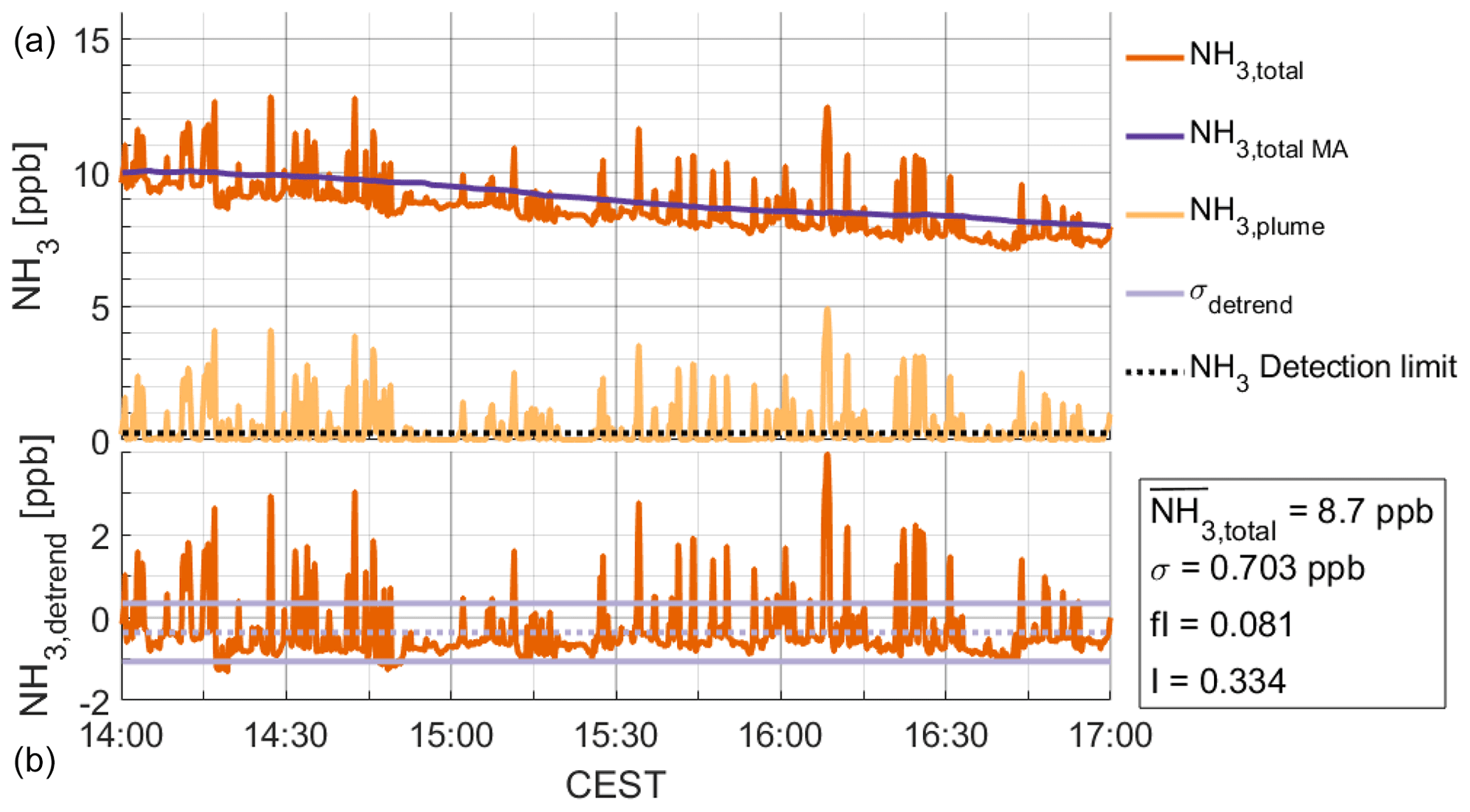
Figure 1Panel (a) shows 10 s time series of NH_3,total (orange) and NH_3,plume (yellow) during the analysis phase, at 250 m from the emission source. The detrended NH_3,total (orange) is shown in panel (b). Fluctuation intensity and intermittency are calculated following Eqs. (4) and (1), respectively, based on the mean NH_3,total, standard deviation (light purple) and NH₃ detection limit (dotted black).

Download

The second variable, fluctuation intensity (fI), determines the magnitude of the NH₃ fluctuations, i.e., NH₃ standard deviation (${\mathit{\sigma }}_{{\mathrm{NH}}_{\mathrm{3}}}$), relative to the mean NH₃ molar fraction ($\stackrel{\mathrm{‾}}{{\mathrm{NH}}_{\mathrm{3}}}$). Fluctuation intensity is defined following Eq. (2):

The fluctuation intensity quantifies the level of turbulent mixing. High fI indicates that there are large fluctuations in the measured NH₃, which can introduce a positive bias in measurements. In the field of plume dispersion, high fI is found close to the source where plume meandering dominates the mixing process (Dosio and Vilà-Guerau de Arellano, 2006), or at the edge of the emission plume as a result of lateral entrainment of air from outside the plume (Mylne and Mason, 1991; Gailis et al., 2007; Ražnjević et al., 2022). When analyzing the fluctuation intensity of NH_3,total, we have a consistent reference for the fluctuation intensity in NH_3,bg. Comparing the fI for the total ammonia (fI_total) to the fI for the background ammonia (fI_bg) enables us to quantify the relative impact of the emitted NH₃ plume to a simulated measurement. When fI_total is of the same order of magnitude as fI_bg, we consider the emission plume indistinguishable from the background NH₃, i.e., the plume is well mixed. Note that for NH_3,plume, the average NH₃ concentration is (very close to) zero outside the emission plume, which could lead to an infinitely large fluctuation intensity following Eq. (2). Therefore, fI is only calculated inside the plume using an arbitrary requirement of $\stackrel{\mathrm{‾}}{{\mathrm{NH}}_{\mathrm{3},\mathrm{plume}}}$ > 10⁻⁵ ppb.

Figure 1 shows a downward trend in NH_3,bg and NH_3,total, resulting from surface deposition and the loss by chemical gas–aerosol transformations. To minimize the impact of this downward trend on ${\mathit{\sigma }}_{{\mathrm{NH}}_{\mathrm{3}}}$, we detrend the simulated molar fraction by subtracting a 1 h leading moving average (NH_3,MA), following Eq. (3) and shown in Fig. 1. The detrended molar fraction (NH_3,detrend) is assumed to only represent turbulent fluctuations and is used to calculate the standard deviation to derive fluctuation intensity. By using NH_3,detrend to calculate ${\mathit{\sigma }}_{{\mathrm{NH}}_{\mathrm{3}}}$, the fluctuation intensity follows from Eq. (4).

Finally, we introduce the 30 min NH₃ flux, studied to mimic the in-field ammonia eddy covariance flux measurements and calculated following Eq. (5). The flux presented in this study is the average 30 min flux for each individual grid point over the analysis phase between 14:00 and 17:00 CEST.

2.4 The concept of blending distance

We use the fluctuation intensity and flux to quantify the impact of the emission plume on the simulated NH₃ molar fraction and flux measurements, by introducing the concept of blending distance. The blending distance is based on the percentage change (PC_X) in the simulated NH₃ measurements resulting from the emission plume, i.e., the percentage change between NH_3,total and NH_3,bg. PC_X is calculated following Eq. (6), where X can be substituted by either fI or F.

Based on this percentage change, we define a threshold for which we assume that the impact of the emission plume is negligible. The blending distance (BD_X) is defined as the maximum distance at which PC_X drops below the threshold level (e.g., PC_X < 25 %), following Eq. (7).

In this study, we present blending distances based on an arbitrary set of threshold levels, ranging from 5 % to 50 %.

The concept of the blending distance is applied to the fluctuation intensity (BD_fI) and the NH₃ flux (BD_F), to quantify the impact on the simulated NH₃ measurements of NH₃ molar fraction and flux, respectively. For context, we also present the intermittency in Sect. 3.2 to quantify the detectability of the plume.

2.5 Blending distance sensitivity

A key aspect of the study is to determine the sensitivity of the concept of the blending distance to variations in meteorological and NH₃ pollution factors. This is in order to study the impact of each process on the blending distance and to identify the driving variables. We study the sensitivity of the blending distance for fluctuation intensity and NH₃ flux by varying the geostrophic wind speed (u_g), initial background molar fraction (C_bg) at the start of the analysis phase, emission strength (E), deposition strength (D), chemical conversion rate (R), simulation height (H) and model grid resolution (Δ). Table 1 presents the suite of numerical experiments in this study. A single numerical experiment was performed for the sensitivity studies of the NH₃ background, emission, deposition and chemistry, each with separate scalars for NH_3,bg and NH_3,plume. This single experiment, which does not include the variations in the geostrophic wind speed nor the high-resolution experiment, generates just under 1 TB of model output with a computational cost of about 64 000 SBU (System Billing Unit, i.e., the usage of one processor of the Cartesius supercomputer system for 1 h).

Table 1Parameter names, symbols, reference values and their respective variations for the sensitivity study of the blending distance, with the reference settings highlighted in bold.

Download Print Version | Download XLSX

The sensitivity study is structured from large-scale processes to small-scale processes and modeling numerics. Starting with mesoscale processes, we vary the geostrophic wind speed to study the impact of the atmospheric stability on blending distance, i.e., a shear or convection-dominated CBL. Atmospheric stability plays a key role in the turbulent mixing of local sources (emission) and sinks (entrainment and deposition), affecting both the fluctuations in the background molar fraction and the mixing of the emission plume (Dosio et al., 2003). Next, we study the sensitivity of BD to different levels of the background NH₃ at the start of the analysis window, representing different levels of regional NH₃ pollution. Additionally, varying the background levels of ammonia changes the NH₃ inversion at the top of the CBL, affecting the impact of entrainment. Next, the emission strength is varied in order to study the local effect of different emission strengths.

Furthermore, we study the sensitivity of both BD_fI and BD_F to NH₃ deposition and the chemical gas–aerosol transformation. These are dynamic processes, i.e., experiencing clear diurnal and seasonal variability, mainly related to temperature, humidity and pollution levels (Wichink Kruit et al., 2010; van Zanten et al., 2010; aan de Brugh et al., 2013). Our simulation approach, with a simplified representation of deposition and chemistry, allows us to distinctly study the role of these two processes.

Finally, we study the sensitivity of BD to choices made in the numerical setup of the experiments. We vary the height of the simulated measurements. The numerical experiments are generally taken at a simulated height of 37.5 m. This is a trade-off between simulating measurements close to the surface to mimic in-field observations and the resolved turbulent kinetic energy (TKE_res) of the model. The TKE_res at the lowest level of DALES (at 2.5 m) is zero due to the no-slip boundary at the surface (Heus et al., 2010). When we aim for a TKE_res of 75 % at all three (vertical) resolutions, we find TKE_res of 76 %, 95 % and 96 % for the low, middle and high resolution at 37.5 m (36.25 m for high resolution). Additionally, it is also expected that varying the measurement height will allow practical insight for in-field observations. Finally, the sensitivity of the blending distance to changes in resolution is studied with two new numerical experiments with higher and lower resolutions of 10 m × 10 m × 2.5 m (1000 × 480 × 1200 grid points) and 50 m × 50 m × 15 m (200 × 96 × 200 grid points), respectively.

3.1 Qualitative analysis of the NH₃ emission plume impact

The concept of blending distance is based on fluctuations in the NH₃ molar fraction. To better understand the sources of these fluctuations, we first study the time series of a “virtual” point measurement at 250 m horizontal distance from the emission source, shown in Fig. 2a. Our simulation framework allows us to distinguish the individual contributions of NH_3,bg (purple) and NH_3,plume (light purple) to NH_3,total (orange). Here we find that the large NH_3,total fluctuations are mainly ascribed to NH_3,plume.

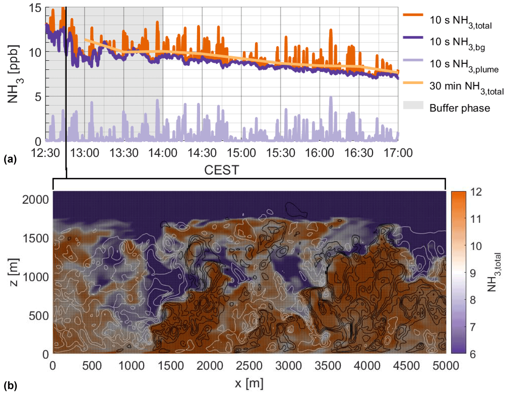
Figure 210 s time series (a) of NH_3,total (orange), NH_3,bg (purple) and NH_3,plume (light purple) during the buffer phase (gray area) and the analysis phase, taken at 250 m distance from the emission source. The large high-frequency fluctuations shown (> 4 ppb) are not captured by the 30 min average of NH_3,total (light orange). The vertical xz cross-section at 12:46 CEST (b) displays high spatial variability during the buffer phase in NH_3,total (> 4 ppb) over short distances (hundreds of meters). The black/white contour lines represent upward/downward wind speeds in steps of 0.5 m s⁻¹.

Download

As discussed in Sect. 2.3, fluctuations are also found in the background molar fraction (NH_3,bg), leading to non-zero fI_bg. Fluctuations NH_3,bg are a result of heterogeneous turbulent mixing. In this study, the fluctuations are caused by vertical gradients only, as we use a homogeneous surface in the simulation of NH_3,bg. These vertical gradients are found near the surface and at the top of the CBL. At the surface, the surface–atmosphere exchange (deposition) decreases the NH₃ molar fraction, which results in a vertical gradient in NH_3,bg. At the top of the CBL, the vertical gradient is a result of the turbulent exchange with the free troposphere (entrainment). Figure 2b shows that the intrusion of NH₃-low air masses from the free troposphere is transported by the downdraft subsidence motions, resulting in large fluctuations in NH_3,bg in the boundary layer. As shown in Fig. 2a, the amplitude of these fluctuations can reach 4 ppb and can last for over 5 min. When averaging over 30 min, even the large fluctuations between 12:30 and 13:15 CEST are filtered out, but these high-frequency turbulent fluctuations could still be present in raw measurement data of high-resolution in-field observations.

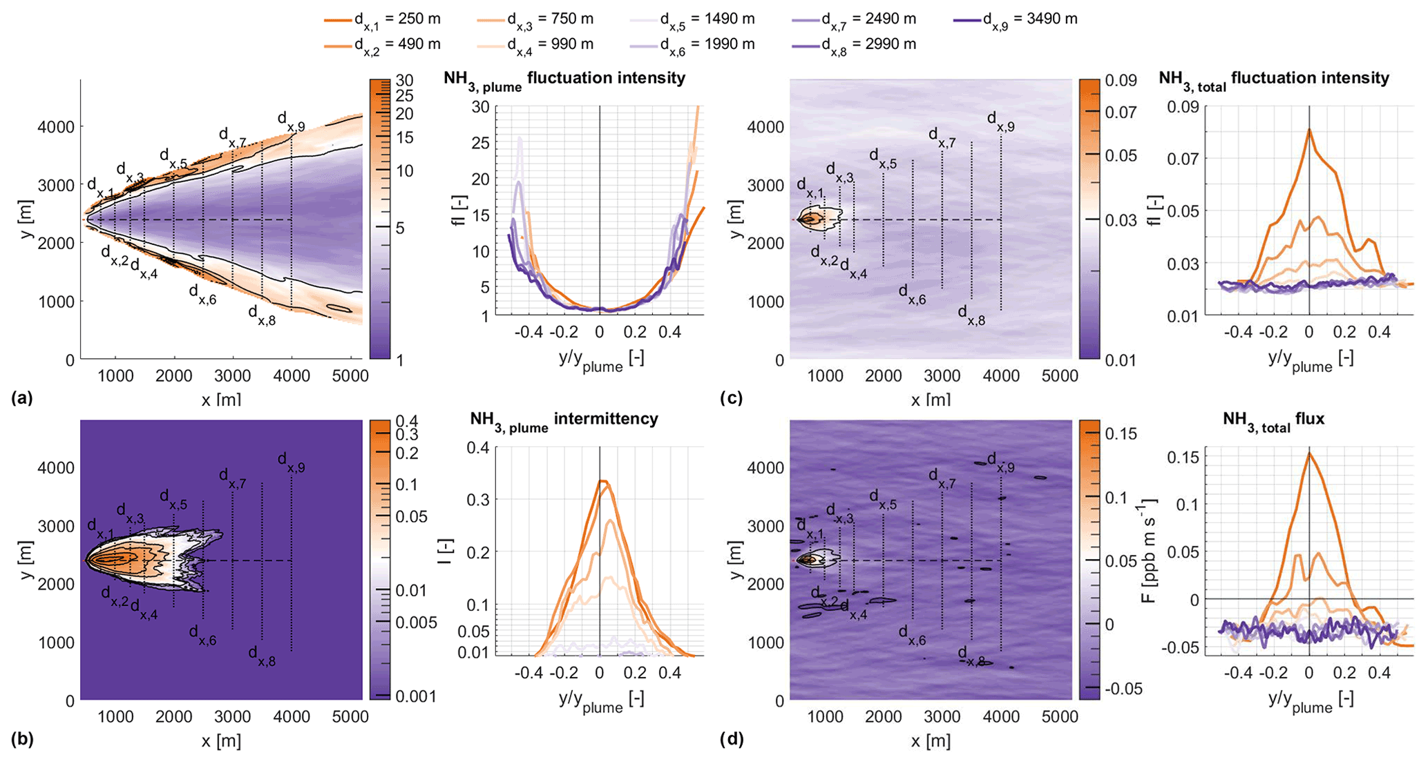
Figure 3The xy cross-sections at 37.5 m with y transects through the NH₃ emission plume for the NH_3,plume fluctuation intensity (a), intermittency (b), NH_3,total fluctuation intensity (c) and NH_3,total flux (d). The plume transects are labeled d_x,1 to d_x,9 for increasing x distance from the NH₃ emission source and normalized by plume width for NH_3,plume > 10⁻⁵ ppb. The data presented are calculated during the analysis phase (14:00 and 17:00 CEST) at 37.5 m.

Download

Now that we understand the source of the NH₃ fluctuations, we take a closer look at the emission plume without any background NH₃. The xy plot in Fig. 3a shows low fI in the plume center (≈ 2) and a strong increase near the plume edges, up to fI ≈ 30. This is echoed by the plume transects, as they show the typical “U-shape” found for Gaussian plumes (Mylne and Mason, 1991; Gailis et al., 2007; Ražnjević et al., 2022). These high fI values at the edges of the plume are a result of very low average molar fractions combined with low intermittency. This leads to a high standard deviation, relative to the very low averaged molar fraction, at the plume edges. Without background NH₃, it is at the edges of the plume that in-plume lateral entrainment of ammonia-free air happens, diluting the emission plume by turbulent mixing.

The intermittency cross-section in Fig. 3b shows that maximum I is only a little over 0.3, resulting from the meandering of the plume. Figure 3b also shows that with an NH₃ detection limit of 0.25 ppb, the plume can be detected up to a distance of about 2.0 km from the source.

The cross-section of fI changes dramatically when analyzing NH_3,total, the sum of NH_3,bg and NH_3,plume. With the addition of a non-zero background molar fraction, fI can be calculated over the whole domain, as shown in Fig. 3c. Now, we find a much lower fluctuation intensity, with a maximum of 0.08 for NH_3,total compared to 30 for NH_3,plume. The U-shape shown in the transect of Fig. 3a is replaced by an approximately Gaussian shape, with the highest fluctuation intensities at the centerline of the plume. This centerline fI decreases with distance from the source and becomes indistinguishable from the out-of-plume fI after approximately 1 km distance, i.e., a rough estimate for BD_fI.

Finally, Fig. 3d shows that the emission plume leads to a positive flux (emission) for NH_3,total in proximity of the emission source, while the flux is negative (deposition) outside the plume. Note that significant fluctuations are found in the flux over the full domain, with ${\mathit{\sigma }}_{F,\mathrm{bg}}=\mathrm{0.0065}$ ppb m s⁻¹ (prescribed $F_{\mathrm{sfc}.}=-\mathrm{0.045}$ ppb m s⁻¹) for NH_3,bg. Similar to fI_total in Fig. 3c, the transects for the NH₃ flux are approximately Gaussian in shape, with peak values close to the plume centerline at $y/y_{\mathrm{plume}}$ = 0. After approximately 1 km at the approximate plume centerline, the in-plume flux becomes visually indistinguishable from the background, i.e., a rough estimate for BD_F. This positive anomaly is the result of the emission source being within the footprint of these receptors.

3.2 Quantitative analysis of the NH₃ emission plume impact

We apply the concept of blending distance in Fig. 4 to the fluctuation intensity (Fig. 4a), flux (Fig. 4b) and intermittency (Fig. 4c). The markers represent the value at each individual grid point on the 37.5 m horizontal plane, the continuous orange line represents the grid point with the highest value within a 50 m moving window (maximum), the orange dotted line represents the plume centerline and the purple dashed and continuous lines represent the blending distances for their respective threshold.

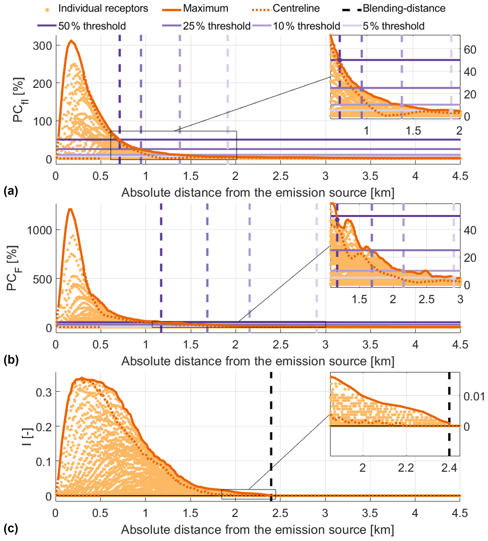
Figure 4The percentage change of NH_3,total relative to NH_3,bg against absolute distance from the NH₃ emission source. The panels show fluctuation intensity (a), NH₃ flux (b) and intermittency (c). The maximum value within a 50 m moving window (orange) and the plume centerline (dotted orange) are highlighted. Blending distances (purple dashed) are calculated based on four thresholds at 5 %, 10 %, 25 % and 50 % (purple continuous).

Download

We interpret the calculation of the blending distance based on four arbitrary threshold levels (5 %, 10 %, 25 % and 50 %) for fI and F, shown in Fig. 4a and b. The distance at which the maximum value of PC_X drops below the threshold level is the blending distance. The sensitivity of BD to these thresholds will be discussed in detail in Sect. 4.1, using Figs. 6 and 7. Additionally, the intermittency in Fig. 4c shows that the emission plume is quantifiable up to over 2.4 km distance.

Starting with the fluctuation intensity (Fig. 4a), PC_fI peaks at a relative change of about 300 %, caused by the NH₃ emission plume. BD_fI decreases nonlinearly from 0.7 to 1.9 km with the thresholds decreasing from 50 % to 5 %. Figure 4b shows that the emission plume has a larger impact on NH₃ flux measurements than on the fluctuation intensity of the NH₃ molar fraction. The large difference between the emission strength (45 ppb m s⁻¹) and the deposition (−0.045 ppb m s⁻¹) results in a maximum PC_F of about 1200 % in close proximity to the emission source. The long tail of PC_F indicates that the turbulent fluctuations in the emission plume affect flux measurements over several kilometers. As a result, BD_F increases from 1.2 to 2.9 km for decreasing thresholds, significantly longer distances than our 1 km qualitative estimate based on Fig. 3d. Note that Fig. 3d shows that the flux change signs in proximity to the emission source and that this sign change is not reflected in Fig. 4b.

Figure 4 shows that the centerline and the maximum statistics give similar results, indicating that the highest values of PC are found at the plume centerline, however, with some variability. These variabilities are visualized in Fig. 5, which shows the spatial structure of the percentage change in grayscale for the fluctuation intensity (PC_fI) in Fig. 5a and the ammonia flux (PC_F) in Fig. 5b. The colored lines in these panels represent the blending distances for different thresholds. The right panels show these same blending distances for different angles from the plume centerline (W), representing different wind directions. Figure 5 shows large variability in the blending distance, especially for the 5 % and 10 % threshold levels, as a result of the chaotic nature of turbulence.

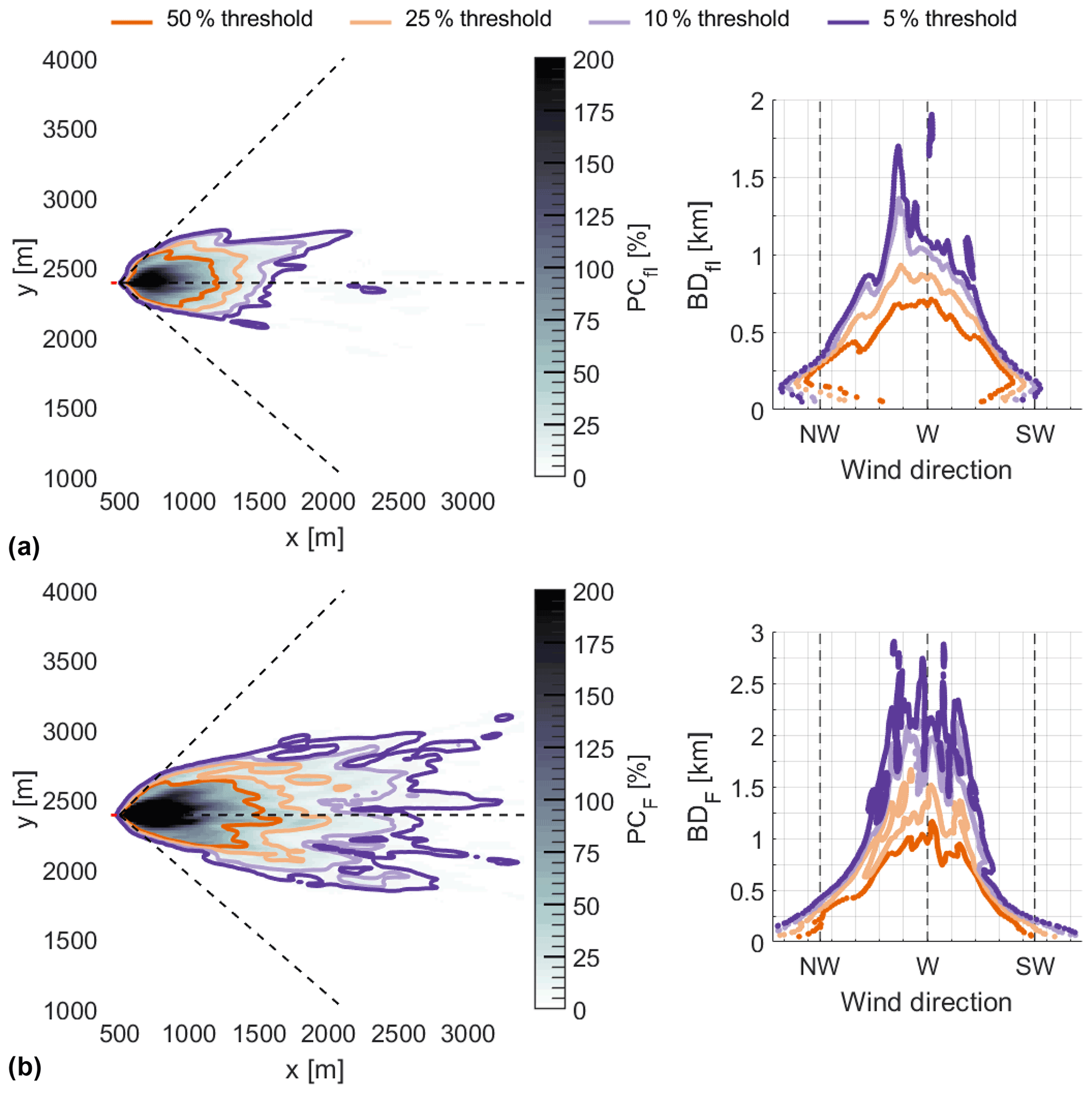
Figure 5The left panels show the spatial structure of the percentage change in grayscale for the fluctuation intensity (PC_fI) in (a) and the ammonia flux (PC_F) in (b). The colored contour lines show the locations where the 50 % (orange), 25 % (light orange), 10 % (light purple) and 5 % (purple) thresholds are met, representing the blending distance (BD). The right panels show these blending distances as a function of different angles from the plume centerline (W), with these angles representing the wind direction.

Download

4.1 The sensitivity of blending distance to meteorological and NH₃ pollution variables

We study the sensitivities of BD_fI and BD_F to a range of meteorological, NH₃ pollution parameters, and model resolution and simulated measurement height (Table 1). The results of the sensitivity study are shown in Figs. 6 and 7, for an arbitrary set of thresholds ranging from 5 % (orange dashed) to 50 % (orange dotted), representing the maximum acceptable difference in fI and F caused by the emission plume in %.

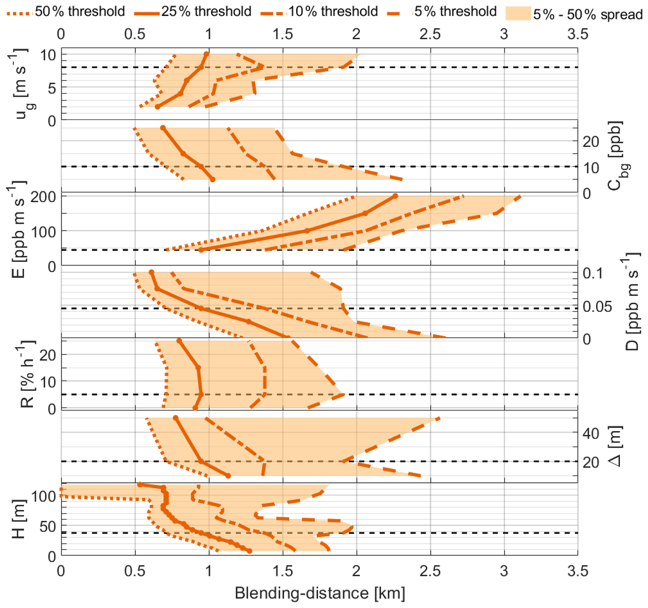
Figure 6The sensitivity of BD_fI to the geostrophic wind speed (u_g), initial background molar fraction (C_bg), emission strength (E), deposition strength (D), chemical reaction rate (R), model resolution (Δ) and simulated measurement height (H). BD_fI is determined for threshold levels ranging from 5 % (orange dashed) to 50 % (orange dotted).

Download

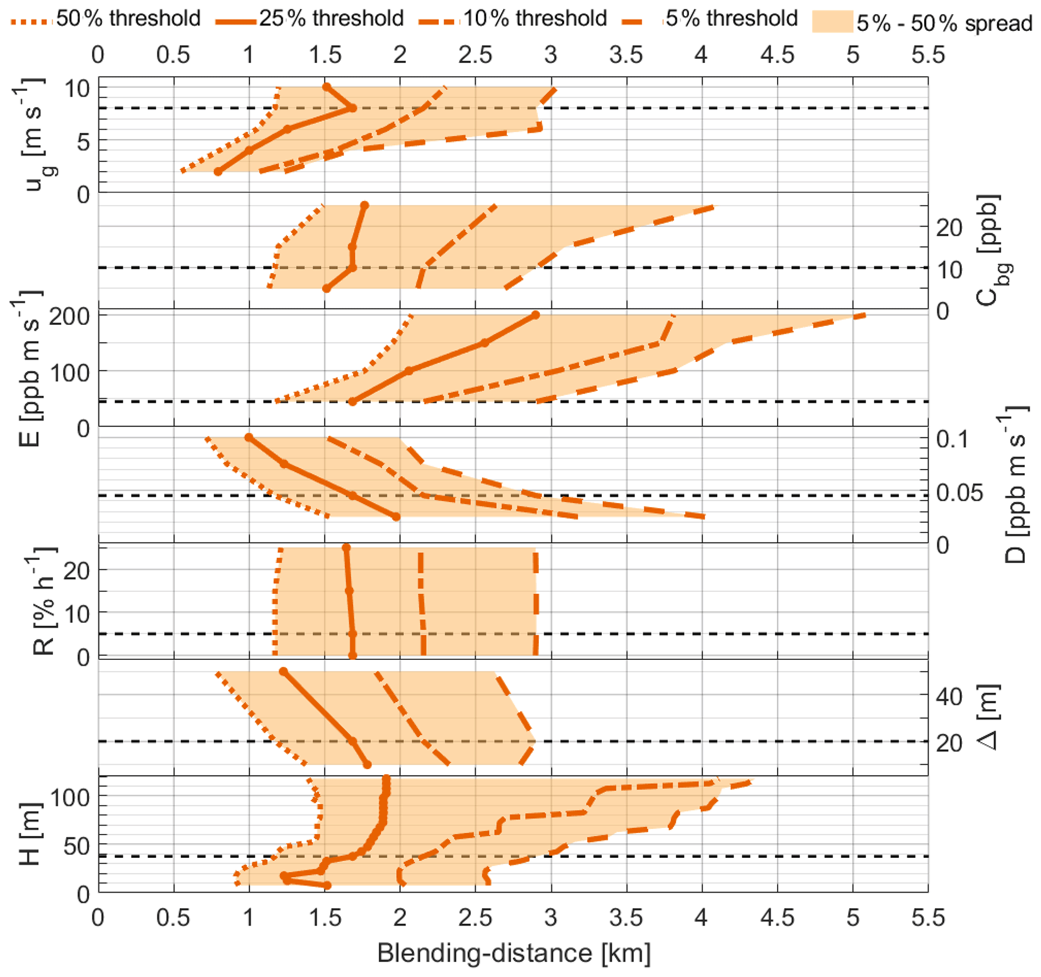
Figure 7The sensitivity of BD_F to the geostrophic wind speed (u_g), initial background molar fraction (C_bg), emission strength (E), deposition strength (D), chemical reaction rate (R), model resolution (Δ) and simulated measurement height (H). BD_F is determined for threshold levels ranging from 5 % (orange dashed) to 50 % (orange dotted).

Download

Starting with BD_fI, Fig. 6 shows that BD_fI ranges roughly between 0.5 and 3.0 km, a first-order estimate of the minimum distance for NH₃ molar fraction measurements. There is a negative correlation between BD_fI and the choice in threshold, i.e., increasing the threshold level decreases BD_fI. We generally find that BD_fI decreases nonlinearly by approximately 1.0 km when increasing the threshold level from 10 % to 50 %, halving BD_fI, highlighted by the large difference between the 10 % (dashed-dotted) and 5 % (dashed) threshold levels for both BD_fI and BD_F. We discuss the individual variables of Fig. 6 from top to bottom, starting at the mesoscale (u_g), down to the micrometer scale (R), and finishing with the model resolution and simulated measurement height.

The geostrophic wind speed (u_g) is one of the main drivers of turbulent mixing and transport of the plume (Dosio et al., 2003; Vrieling and Nieuwstadt, 2003; Dosio and Vilà-Guerau de Arellano, 2006). Figure 6 shows a positive correlation between BD_fI and u_g. By varying u_g, we move from a convection-driven boundary layer (u_g = 2 m s⁻¹) to more shear-driven meteorological conditions (u_g = 10 m s⁻¹). In a convection-driven boundary layer, turbulent mixing is rather weak and the NH₃ emission plume rises from the surface as convection plumes are the main drivers of turbulent mixing. Under these conditions, in-plume molar fractions are very high, but horizontal transport of the emission plume is weak, resulting in a low BD_fI. For shear-driven conditions, the NH₃ emission plume tends to stick to the surface as the increased horizontal wind speed enhances horizontal transport and turbulent mixing. The enhanced horizontal transport and emission plume sticking to the surface should significantly increase BD_fI, but the enhanced turbulent mixing counteracts these processes by reducing the NH_3,plume molar fraction and fluctuations. This is shown in Fig. 6 and explains why the sensitivity of BD_fI increases for lower threshold levels (5 %), as smaller plume fluctuations will reach long distances in shear-driven conditions.

One panel below, Fig. 6 shows a negative correlation between BD_fI and the initial background molar fraction (C_bg), i.e., the regional level of NH₃ pollution. The first cause of the negative correlation is the higher average molar fraction, which lowers the relative weight of the NH_3,plume fluctuations (σ_plume) when fI_total is calculated following Eq. (2). Additionally, increasing NH_3,bg leads to a large difference in the NH₃ air mass characteristics at the top of the boundary layer. The exchange between the boundary layer and free tropospheric air masses through entrainment increases σ_bg at 37.5 m from 0.13 ppb (C_bg = 5 ppb) to 0.38 ppb (C_bg = 25 ppb), resulting in an increased fI_bg. Both processes reduce the magnitude of PC_fI for increasing C_bg, resulting in a decrease of BD_fI.

At the local scale, Fig. 6 shows a clear positive and negative correlation when varying emission strength (E) and deposition strength (D), respectively. Both variables directly affect one of the main drivers of turbulent mixing – heterogeneity. Increasing the NH₃ emission strength of the local (heterogeneous) source directly increases fI_plume, increasing BD_fI. Varying the deposition, on the other hand, directly affects the vertical gradient of the NH₃ molar fraction near the surface, increasing fI_bg for increasing D and therefore reducing BD_fI.

We only briefly touch upon the chemical conversion rate (R), as Fig. 6 shows that varying R does not significantly affect BD_fI. R is applied uniformly to the 3D domain and has little effect on turbulent mixing. Note that our simplified representation of chemistry could lead to a potential underestimation of the impact of chemistry on BD_fI, as our approach is unable to resolve potential nonlinear effects of turbulent mixing on the in-plume chemical reaction rate near the emission source (see discussion in Sect. 4.2).

Next, we vary the model resolution (Δ) in Fig. 6 and find that BD_fI is weakly sensitive to the model resolution. The results indicate that the calculation of the blending distance does benefit by increasing the simulation resolution. However, there is a trade-off between the computational costs of the simulation and the resolution.

Finally, Fig. 6 shows two regimes in the sensitivity of BD_fI to the simulated measurement height (H). For the 50 % threshold, BD decreases by about 500 m with height up to 90 m. Above 90 m, there is a transition where BD_fI rapidly goes to zero. In this second regime, the simulated measurements are located above the plume centerline. Thereon, fI_plume rapidly decreases in height until PC_fI does not reach the 50 % threshold and BD_fI becomes zero. This rapid decrease is a result of the simulated measurements being located above the emission plume, as the height of the plume does not reach above 150 m for the first 1.5 km horizontal distance. The height of this transition increases with decreasing threshold levels as the thresholds become more sensitive to smaller NH_3,plume fluctuations.

Figure 7 shows the results of the sensitivity study for BD_F (Table 1). Both the blending distance for molar fraction measurements (BD_fI) and for flux measurements (BD_F) can be interpreted as an inverse footprint analysis, as we estimate the area affected by the emission source. The results of the sensitivity study of BD_F, however, are different from the BD_fI results, as the footprints for flux and molar fraction measurements are not the same. The footprint for flux measurements is smaller than those of molar fraction measurements (Rannik et al., 2000; Kljun et al., 2003; Vesala et al., 2008). However, comparing BD_fI to the footprint of NH₃ molar fraction measurements is not straightforward, as BD_fI is based on the NH₃ fluctuation intensity, not the molar fraction. It is therefore interesting to determine whether the results of the sensitivity study of BD_F will differ compared to the results of BD_fI.

When analyzing Fig. 7, we find that there are indeed differences between BD_F and BD_fI. BD_F is significantly longer, ranging from 0.75 to roughly 5 km, indicating that NH₃ flux measurements are more sensitive to the emission plume. Note that we removed the results for D = 0 ppb m s⁻¹. Here, F_bg approaches zero, resulting in infinitely large PC_F and unrealistic BD_F values, following Eq. (6).

One of main differences between BD_F and BD_fI is found in the sensitivity to the threshold levels (5 % to 50 %). BD_F is more sensitive to the different threshold levels compared to BD_fI. This is in agreement with the results shown in Fig. 4b, where we discussed that PC_F is significantly larger than PC_fI, with a longer tail. As a result, the nonlinear effect of the aforementioned long tail in PC_F (Fig. 4b) increases BD_F for low threshold levels. Despite these differences, the same arbitrary set of thresholds is used for both BD_fI and BD_F.

Significant differences between BD_F and BD_fI are also found in the sensitivity to the geostrophic wind speed (u_g) and the simulated measurement height (H). Both variables directly affect the footprint of the simulated flux measurements. In shear-driven turbulent conditions (high u_g), the footprint of the measurement is elongated compared to convective conditions. This reduces the width of the footprint and lengthens the up-wind distance at which the emission source can be measured, thus, increasing BD_F. Increasing H also increases the footprint of the measurements, but there is no elongation of the footprint. As a result, BD_F has a strong positive correlation to u_g, but is only weakly correlated to H, except for the lower threshold levels.

Figure 7 appears to show that BD_F has a weak positive correlation with increasing C_bg. This is mainly attributed to an increase in the spatial variations of the background NH₃ flux, which increases from ${\mathit{\sigma }}_{F,\mathrm{bg}}=\mathrm{0.0065}$ ppb m s⁻¹ for C_bg = 10 ppb (Fig. 3d) to ${\mathit{\sigma }}_{F,\mathrm{bg}}=\mathrm{0.015}$ for C_bg = 25 ppb. As a result, the fluctuations in PC_F shown in Fig. 4b, increase in amplitude and frequency, which particularly affects the low threshold levels of 5 % and 10 %.

There are also strong similarities between the sensitivity of BD_F and BD_fI. Both Figs. 6 and 7 show that the blending distance is only weakly sensitive to the chemical reaction rate (R) and the model resolution (Δ). For both molar fraction and flux measurements, the emission strength (E), deposition (D) and, to a lesser extent, the geostrophic wind speed (u₃) are the driving variables of the blending distance.

4.2 Uncertainty of the blending distance estimation

The turbulent dispersion of the emission plume is chaotic by nature and driven by a wide range of factors. We therefore carry out a systematic analysis on how these factors and the model resolution influence the relationships between emissions and simulated in-field measurements. The chaotic nature of turbulence results in random variations in both the emitted NH₃ (Fig. 3a and b) and the background NH₃ (Fig. 3c and d). These random fluctuations lead to variability in the calculation of the blending distances, leading to uncertainty in the blending distances presented in this study. The variability increases when using the lower threshold levels (e.g., 5 % and 10 %), as is visualized and discussed in Sect. 3.1 and 3.2. The variability could be reduced by increasing the length of the analysis window, i.e., increasing the averaging time to filter out the small and short spatio-temporal turbulence variability.

Increasing the length analysis window, however, means that the blending distance is calculated using a wider range of boundary layer dynamics and variations in the thermodynamic variables. Boundary layer dynamics are especially relevant in the morning and early afternoon when the boundary layer grows and air from the residual layer and free troposphere is entrained, or in the afternoon when turbulence decays (Pino et al., 2006). It leads to entrainment being one of the dominant processes driving the NH₃ diurnal variability (Wichink Kruit et al., 2007; Schulte et al., 2021). In Fig. 2, we show that it leads to large fluctuations in NH_3,bg, significantly increasing fI_bg. We therefore filter out the impact of boundary layer dynamics and variations in the thermodynamic variables with our choice of analysis window from 14:00 and 17:00 CEST, in order to find a first-order estimate of the blending distance. We do recommend a follow-up study on the role of boundary dynamics.

Finally, there is a downside to our simplified representation of chemical transformations in that it is applied uniformly to the 3D domain. In reality, the equilibrium molar fractions for these chemical transformations are related to temperature and humidity, and results in a near-surface NH₃ gradient of the NH₃ molar fraction (aan de Brugh et al., 2013). Therefore, we are likely to underestimate the role of chemical transformations and overestimate BD_fI, as turbulent mixing of this near-surface gradient increases fI_bg.

The blending distance cannot be captured by a single number. This is partly due to the uncertainty involved in calculating the blending distance, but the blending distances is, most of all, an integrated variable. Several processes are captured by the blending distance in one single variable, including the chaotic nature of turbulent plume dispersion, convective and shear-induced turbulence, atmospheric pollution levels and surface heterogeneity. As shown in Sect. 4.1, each of these processes impacts the blending distance differently. Despite its complexity, the blending distance is a useful variable since it is an integrated variable; all the aforementioned processes are represented in this distance at which the impact of an emission plume is negligible with respect to the background.

The applicability of the results presented here depends not only on the meteorological and NH₃ pollution factors, but also on the physical context of the measurement site. This study is based on the Ruisdael CESAR Observatory at Cabauw, which is located on flat agricultural grassland with surface elevation changing only by a few meters over 20 km. A different physical context, like a heterogeneous surface which changes turbulent properties (Ouwersloot et al., 2011), is likely to significantly affect the resulting blending distances. With the simulation framework presented here, the blending distance can be calculated for specific weather conditions and for the physical context of the measurement site, providing a more accurate assessment of the impact of nearby emissions on NH₃ observations at a specific measurement site. The results presented in this study provide a valuable first estimate of and discussion on a typical blending distance and its driving variables.

4.3 Blending distance literature for passive tracers

Evaluating the blending distance results against typical literature on plume dispersion is a difficult exercise. The topic is generally not mentioned as these studies focus on the release of passive scalars in an unpolluted environment, and only few studies even research (near) surface releases (Cassiani et al., 2020). Normalization of both distance from the source and the in-plume molar fraction further complicates the interpretation of literature results.

We therefore try to estimate the order of magnitude of the blending distance based on the in-plume molar fraction and fluctuation intensity of plume dispersion modeling studies. Following figures by Dosio et al. (2003) and Dosio and Vilà-Guerau de Arellano (2006), we find that the in-plume molar fraction rapidly decreases for a convection-driven boundary layer ($-z/L$ ≥ 40 and $u_{*}/w_{*}$ ≤ 0.2) at the surface up to roughly 6 km distance, after which, it starts to level off. Similar results are found for the fluctuation intensity; however, the results are less pronounced for the near-surface release experiments. The 6 km distance approximately doubles for shear-driven boundary layers ($-z/L$ ∼ 40 and $u_{*}/w_{*}$ ∼ 0.46). The observations shown in Fig. 10 by Mylne and Mason (1991) show that the observed fluctuation intensity also decreases with distance, but levels after roughly 15 km distance from the emission source. We use these distances at which the plume statistics start to level off as an estimate of the order of magnitude of the blending distance, indicating that the blending distance could be in the order of several kilometers (6 to 15 km), based on plume dispersion literature.

These rough estimates of the 6 to 15 km distance are significantly larger than the blending distances presented in this study. Such long distances between source and measurement site would not make feasible requirements in densely agricultural regions, but are likely an overestimation of the blending distance. These estimates are based on the molar fraction and fI of the emission plume, with no representation of background ammonia levels. The latter is especially important, as we show in Sect. 3.1 and 3.2 that the impact of the emission plume rapidly decreases relative to the turbulent background ammonia, while the emission plume itself can be detected for several kilometers as indicated by the intermittency.

4.4 Blending distance literature for ammonia measurements

Articles on ammonia measurements in close proximity to an emission source implicitly include all relevant processes. These studies could also provide a qualitative, perhaps more realistic, evaluation of the NH₃ blending distance results presented here. In-field measurements show that the NH₃ molar fraction exponentially decreases with distance from the source, with measurements close to the background molar fraction after 300 to 500 m (Fowler et al., 1998; Sommer et al., 2009; Shen et al., 2016). Similar results were obtained in an intercomparison study of short-range atmospheric dispersion models by Theobald et al. (2012), at horizontal resolutions of 25–50 m and receptors at 100 m intervals along four radial directions (N, E, S and W). However, these measurements are typically arranged a few lines downwind of the source, with only a handful of measurements over a distance of 300 to 1000 m. At these short distances, plume dispersion is dominated by meandering of the plume (Nieuwstadt, 1992), and the in-plume molar fraction measurements are underestimated as a result, especially given the averaging times of these measurements ranging from several hours up to multiple weeks.

Finally, we can evaluate our findings against measurement site requirements of air quality networks. The Dutch air quality network and the EMEP (European Monitoring and Evaluation Programme) network do set requirements for the minimum distance from emission sources and no references to scientific studies are provided. Back in 1990, the Dutch network required a minimum distance for NH₃ sites of 300–500 m from NH₃ point or area sources, depending on source strength (Boermans and Erisman, 1990). This is in line with the literature on measurements in proximity to emission sources discussed earlier, but closer than the blending distances presented here. Currently, no hard requirements are in place in the Netherlands, although the potential impact of NH₃ sources is still recognized (Wichink Kruit et al., 2021). At a European level, EMEP measurement sites require a 2 km minimum distance for measurements nearby the stabling of animals and manure applications, depending on the number of animals and field size (Schaug, 1988; EMEP/CCC, 2001). This 2 km distance is in line with our recommendations, although the results in this study indicate that distances below 2 km could also be sufficient.

4.5 Towards an NH₃ virtual test bed: integrating fine-scale simulations with advanced observations

This study is the first that specifically addresses the regional representativity of ammonia measurements in proximity to an emission source. The systematic analysis presented in Figs. 6 and 7 can be used as a reference when interpreting in-field NH₃ measurements. Additionally, the simulation framework can be applied to individual locations to study the representativity of (potential new) measurement sites under local conditions by using the concept of blending distance. One can expand the simulation framework to include multiple sources, area sources – each with a unique passive scalar – and heterogeneous surface conditions (Ouwersloot et al., 2011) to simulate local NH₃ conditions.

The DALES model proved to be flexible, allowing for simulations of a convective, sheared convective, stable and cloud-topped boundary layer (Verzijlbergh et al., 2009; Heus et al., 2010). The fine-scale simulation framework will be included in the Ruisdael CESAR Observatory at Cabauw, a nationwide observatory for measurements and modeling of the atmosphere and air quality. It can be a powerful tool in future ammonia research, e.g., in preparation of (emission) measurement campaigns or to improve interpretation of NH₃ (flux) measurements. Furthermore, we want to stress that the methods presented here are not limited to ammonia, but can be used for any gas for which relevant processes occur at high spatio-temporal resolutions.

We recommend expanding the simulation framework to create a testbed to study NH₃ at high spatio-temporal resolutions, including all processes relevant to the NH₃ diurnal variability. The main additions should be a dynamic parameterization of the surface–atmosphere exchange, e.g., DEPAC (van Zanten et al., 2010) and a thermodynamic chemistry module, e.g., ISORROPIA version 2 (Fountoukis and Nenes, 2007). With these additions, on top of the existing possibility to distinguish between background and emitted NH₃, the fine-scale simulation framework with explicitly resolved turbulence will be well suited to study short-range dispersion of ammonia, e.g., deposition in close proximity to emission sources and the impact of turbulent micromixing on the chemical reaction rate. These studies are typically performed using models where turbulence is parameterized or Gaussian plume models are used (Loubet et al., 2006; Sommer et al., 2009; van der Swaluw et al., 2017). Furthermore, the addition of a thermodynamic chemistry module can lead to new insights on NH₃ flux measurements. The equilibrium molar fractions of the NH₃ gas–aerosol transformations depend on atmospheric temperature and humidity, resulting in a near-surface molar fraction gradient. This gradient leads to an underestimation of the NH₃ deposition flux of about 0.02 µg m⁻² s⁻¹, when using the flux-gradient method (Nemitz et al., 2004). With these additions to the simulation framework, the virtual NH₃ testbed can be used improve the interpretation of NH₃ flux measurements.