Page 1 PROBLEM 3.1 KNOWN: One-dimensional, plane wall ...

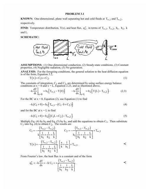
PROBLEM 3.1KNOWN: One-dimensional, plane wall separating hot and cold fluids at T ∞,1 and T∞ ,2,respectively.FIND: Temperature distribution, T(x), and heat flux, q′′x , in terms of T ∞,1 , T ∞,2, h1, h 2 , kand L.SCHEMATIC:ASSUMPTIONS: (1) One-dimensional conduction, (2) Steady-state conditions, (3) Constantproperties, (4) Negligible radiation, (5) No generation.ANALYSIS: For the foregoing conditions, the general solution to the heat diffusion equationis of the form, Equation 3.2,T x = C x+ C .(1)( ) 1 2The constants of integration, C 1 and C 2 , are determined by using surface energy balanceconditions at x = 0 and x = L, Equation 2.23, and as illustrated above,dT ⎤dT ⎤− k h1 T∞,1 T( 0 ) k h2 T( L)T ∞,2.dt ⎥= ⎡⎣− ⎤⎦− = ⎡ − ⎤x=0 dx ⎥ ⎣ ⎦(2,3)⎦⎦x=LFor the BC at x = 0, Equation (2), use Equation (1) to find− k( C1+ 0) = h1 ⎡⎣T∞,1−( C1⋅ 0+C2)⎤⎦(4)and for the BC at x = L to find( ) ⎡( )− k C1+ 0 = h2⎣C1L+ C2 −T ∞,2⎤⎦.(5)Multiply Eq. (4) by h 2 and Eq. (5) by h 1 , and add the equations to obtain C 1 . Then substituteC 1 into Eq. (4) to obtain C 2 . The results are( T∞,1 −T∞,2 ) ( T∞,1 −T∞,2)C 1 =− C2 =− + T∞,1⎡ 1 1 L⎤ ⎡ 1 1 L⎤k⎢ + + h1h1 h2 k⎥ ⎢ + +h1 h2k⎥⎣ ⎦ ⎣ ⎦( T∞,1 − T∞,2) ⎡x 1 ⎤T( x ) =− ⎢ + ⎥+T ∞,1.

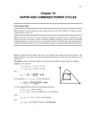
PROBLEM 3.2KNOWN: Temperatures and convection coefficients associated with air at the inner and outer surfacesof a rear window.FIND: (a) Inner and outer window surface temperatures, T s,i and T s,o , and (b) T s,i and T s,o as a function ofthe outside air temperature T ∞,o and for selected values of outer convection coefficient, h o .SCHEMATIC:ASSUMPTIONS: (1) Steady-state conditions, (2) One-dimensional conduction, (3) Negligible radiationeffects, (4) Constant properties.PROPERTIES: Table A-3, Glass (300 K): k = 1.4 W/m⋅K.ANALYSIS: (a) The heat flux may be obtained from Eqs. 3.11 and 3.12,( )$ $T40 C 10 C∞,i − T− −∞,oq′′ = =1 L 1 1 0.004 m 1+ + + +h 2 2o k hi65 W m ⋅K 1.4 W m ⋅ K 30 W m ⋅K50 C2q′′ = = 968W m .20.0154 + 0.0029 + 0.0333 m ⋅K W( )Hence, with q h ( T T )$′′ = i ∞,i − ∞,o, the inner surface temperature is2q′′968W mTs,i = T∞,i − h = 40 C − = 7.7 C2i 30 W m ⋅ K$ $

PROBLEM 3.2 (Cont.)Surface temperatures, Tsi or Tso (C)403020100-10-20-30-30 -25 -20 -15 -10 -5 0Outside air temperature, Tinfo (C)Tsi; ho = 100 W/m^2.KTso; ho = 100 W/m^2.KTsi; ho = 65 W/m^2.KTso; ho = 65 W/m^2.KTsi or Tso; ho = 2 W/m^.KCOMMENTS: (1) The largest resistance is that associated with convection at the inner surface. Thevalues of T s,i and T s,o could be increased by increasing the value of h i .(2) The IHT Thermal Resistance Network Model was used to create a model of the window and generatethe above plot. The Workspace is shown below.// Thermal Resistance Network Model:// The Network:// Heat rates into node j,qij, through thermal resistance Rijq21 = (T2 - T1) / R21q32 = (T3 - T2) / R32q43 = (T4 - T3) / R43// Nodal energy balancesq1 + q21 = 0q2 - q21 + q32 = 0q3 - q32 + q43 = 0q4 - q43 = 0/* Assigned variables list: deselect the qi, Rij and Ti which are unknowns; set qi = 0 for embedded nodal pointsat which there is no external source of heat. */T1 = Tinfo // Outside air temperature, C//q1 =// Heat rate, WT2 = Tso // Outer surface temperature, Cq2 = 0// Heat rate, W; node 2, no external heat sourceT3 = Tsi// Inner surface temperature, Cq3 = 0// Heat rate, W; node 2, no external heat sourceT4 = Tinfi // Inside air temperature, C//q4 =// Heat rate, W// Thermal Resistances:R21 = 1 / ( ho * As )R32 = L / ( k * As )R43 = 1 / ( hi * As )// Convection thermal resistance, K/W; outer surface// Conduction thermal resistance, K/W; glass// Convection thermal resistance, K/W; inner surface// Other Assigned Variables:Tinfo = -10 // Outside air temperature, Cho = 65// Convection coefficient, W/m^2.K; outer surfaceL = 0.004 // Thickness, m; glassk = 1.4// Thermal conductivity, W/m.K; glassTinfi = 40 // Inside air temperature, Chi = 30// Convection coefficient, W/m^2.K; inner surfaceAs = 1// Cross-sectional area, m^2; unit area

PROBLEM 3.3KNOWN: Desired inner surface temperature of rear window with prescribed inside and outside airconditions.FIND: (a) Heater power per unit area required to maintain the desired temperature, and (b) Compute andplot the electrical power requirement as a function of T ∞ ,o for the range -30 ≤ T ∞ ,o ≤ 0°C with h o of 2,20, 65 and 100 W/m 2 ⋅K. Comment on heater operation needs for low h o . If h ~ V n , where V is thevehicle speed and n is a positive exponent, how does the vehicle speed affect the need for heateroperation?SCHEMATIC:ASSUMPTIONS: (1) Steady-state conditions, (2) One-dimensional heat transfer, (3) Uniform heaterflux, q′′ h , (4) Constant properties, (5) Negligible radiation effects, (6) Negligible film resistance.PROPERTIES: Table A-3, Glass (300 K): k = 1.4 W/m⋅K.ANALYSIS: (a) From an energy balance at the inner surface and the thermal circuit, it follows that for aunit surface area,T∞,i −Ts,i Ts,i −T∞,o+ q′′h =1h Lk+1hio( )$ $Ts,i T ,o T ,i T 15 C − −10 C$ $− ∞ ∞ − s,i25 C −15 Cq′′ h = − = −Lk+1h 0.004 m 1 1o 1hi+1.4 W m ⋅ K 2 265 W m ⋅ K 10 W m ⋅ K′′2 2= ( − ) =

T∞,i − Ts,i 1hi0.10= = = 0.846,T∞,i − T∞,o 1hi + Lk+1ho0.118or s,i( )$ $ $T = 25C− 0.84635C = −4.6C.

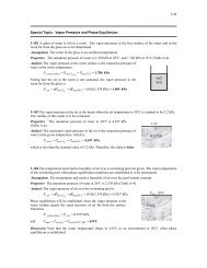
PROBLEM 3.4KNOWN: Curing of a transparent film by radiant heating with substrate and film surface subjected toknown thermal conditions.FIND: (a) Thermal circuit for this situation, (b) Radiant heat flux, q′′ o (W/m 2 ), to maintain bond atcuring temperature, T o , (c) Compute and plot q′′ o as a function of the film thickness for 0 ≤ L f ≤ 1 mm,and (d) If the film is not transparent, determine q′′ o required to achieve bonding; plot results as a functionof L f .SCHEMATIC:ASSUMPTIONS: (1) Steady-state conditions, (2) One-dimensional heat flow, (3) All the radiant heatflux q′′ o is absorbed at the bond, (4) Negligible contact resistance.ANALYSIS: (a) The thermal circuitfor this situation is shown at the right.Note that terms are written on a per unitarea basis.(b) Using this circuit and performing an energy balance on the film-substrate interface,Tq′′ o = q1′′ + q′′o −T To T12q∞ −′′ o = +R′′ cv + R′′ f Rs′′where the thermal resistances are2 2R′′ cv = 1 h = 1 50 W m ⋅ K = 0.020 m ⋅K W2R′′ f = Lf kf= 0.00025 m 0.025 W m ⋅ K = 0.010 m ⋅K W2R′′ s = Ls ks= 0.001m 0.05 W m ⋅ K = 0.020 m ⋅K W( − )[ ]( − )$ $60 20 C 60 30 C2 2q′′ o = + = ( 133 + 1500)W m = 2833W m2 20.020 + 0.010 m ⋅K W 0.020 m ⋅K W

PROBLEM 3.4 (Cont.)7000Radiant heat flux, q''o (W/m^2)600050004000300020000 0.2 0.4 0.6 0.8 1Film thickness, Lf (mm)Opaque filmTransparent filmCOMMENTS: (1) When the film is transparent, the radiant flux is absorbed on the bond. The fluxrequired decreases with increasing film thickness. Physically, how do you explain this? Why is therelationship not linear?(2) When the film is opaque, the radiant flux is absorbed on the surface, and the flux required increaseswith increasing thickness of the film. Physically, how do you explain this? Why is the relationshiplinear?(3) The IHT Thermal Resistance Network Model was used to create a model of the film-substrate systemand generate the above plot. The Workspace is shown below.// Thermal Resistance NetworkModel:// The Network:// Heat rates into node j,qij, through thermal resistance Rijq21 = (T2 - T1) / R21q32 = (T3 - T2) / R32q43 = (T4 - T3) / R43// Nodal energy balancesq1 + q21 = 0q2 - q21 + q32 = 0q3 - q32 + q43 = 0q4 - q43 = 0/* Assigned variables list: deselect the qi, Rij and Ti which are unknowns; set qi = 0 for embedded nodal pointsat which there is no external source of heat. */T1 = Tinf // Ambient air temperature, C//q1 =// Heat rate, W; film sideT2 = Ts// Film surface temperature, Cq2 = 0// Radiant flux, W/m^2; zero for part (a)T3 = To// Bond temperature, Cq3 = qo// Radiant flux, W/m^2; part (a)T4 = Tsub // Substrate temperature, C//q4 =// Heat rate, W; substrate side// Thermal Resistances:R21 = 1 / ( h * As )R32 = Lf / (kf * As)R43 = Ls / (ks * As)// Convection resistance, K/W// Conduction resistance, K/W; film// Conduction resistance, K/W; substrate// Other Assigned Variables:Tinf = 20// Ambient air temperature, Ch = 50// Convection coefficient, W/m^2.KLf = 0.00025 // Thickness, m; filmkf = 0.025 // Thermal conductivity, W/m.K; filmTo = 60// Cure temperature, CLs = 0.001 // Thickness, m; substrateks = 0.05 // Thermal conductivity, W/m.K; substrateTsub = 30 // Substrate temperature, CAs = 1// Cross-sectional area, m^2; unit area

PROBLEM 3.5KNOWN: Thicknesses and thermal conductivities of refrigerator wall materials. Inner and outer airtemperatures and convection coefficients.FIND: Heat gain per surface area.SCHEMATIC:ASSUMPTIONS: (1) One-dimensional heat transfer, (2) Steady-state conditions, (3) Negligiblecontact resistance, (4) Negligible radiation, (5) Constant properties.ANALYSIS: From the thermal circuit, the heat gain per unit surface area isT∞,o − T∞,iq′′ =( 1/hi) + ( L p /kp) + ( L i/ki) + ( L p /kp) + ( 1/ho)( )25− 4 ° Cq′′ =2 1/ 5W / m K 2 0.003m / 60 W / m K 0.050m / 0.046 W / m K2( ⋅ ) + ( ⋅ ) + ( ⋅ )21°Cq′′ = = 14.1 W / m20.4 + 0.0001+ 1.087 m2⋅K / W( )COMMENTS: Although the contribution of the panels to the total thermal resistance is negligible,that due to convection is not inconsequential and is comparable to the thermal resistance of theinsulation.

PROBLEM 3.6KNOWN: Design and operating conditions of a heat flux gage.FIND: (a) Convection coefficient for water flow (T s = 27°C) and error associated with neglectingconduction in the insulation, (b) Convection coefficient for air flow (T s = 125°C) and error associatedwith neglecting conduction and radiation, (c) Effect of convection coefficient on error associated withneglecting conduction for T s = 27°C.SCHEMATIC:ASSUMPTIONS: (1) Steady-state, (2) One-dimensional conduction, (3) Constant k.ANALYSIS: (a) The electric power dissipation is balanced by convection to the water and conductionthrough the insulation. An energy balance applied to a control surface about the foil therefore yieldsHence,( ) ( )Pelec ′′ = q′′ conv + q′′cond = h Ts − T∞+ k Ts −TbL2Pelec ′′ −k ( Ts −Tb) L 2000 W m −0.04 W m ⋅K( 2 K)0.01mh = =Ts− T∞2K2( 2000 − 8)W m2h = = 996 W m ⋅ K

PROBLEM 3.6 (Cont.)If conduction, radiation, or conduction and radiation are neglected, the corresponding values of h and thepercentage errors are 18.5 W/m 2 ⋅K (27.6%), 16 W/m 2 ⋅K (10.3%), and 20 W/m 2 ⋅K (37.9%).(c) For a fixed value of T s = 27°C, the conduction loss remains at q′′ cond = 8 W/m 2 , which is also thefixed difference between P′′ elec and q′′ conv . Although this difference is not clearly shown in the plot for10 ≤ h ≤ 1000 W/m 2 ⋅K, it is revealed in the subplot for 10 ≤ 100 W/m 2 ⋅K.2000200Power dissipation, P''elec(W/m^2)1600120080040000 200 400 600 800 1000Power dissipation, P''elec(W/m^2)160120804000 20 40 60 80 100Convection coefficient, h(W/m^2.K)Convection coefficient, h(W/m^2.K)No conductionWith conductionNo conductionWith conductionErrors associated with neglecting conduction decrease with increasing h from values which aresignificant for small h (h < 100 W/m 2 ⋅K) to values which are negligible for large h.COMMENTS: In liquids (large h), it is an excellent approximation to neglect conduction and assumethat all of the dissipated power is transferred to the fluid.

PROBLEM 3.7KNOWN: A layer of fatty tissue with fixed inside temperature can experience differentoutside convection conditions.FIND: (a) Ratio of heat loss for different convection conditions, (b) Outer surfacetemperature for different convection conditions, and (c) Temperature of still air whichachieves same cooling as moving air (wind chill effect).SCHEMATIC:ASSUMPTIONS: (1) One-dimensional conduction through a plane wall, (2) Steady-stateconditions, (3) Homogeneous medium with constant properties, (4) No internal heatgeneration (metabolic effects are negligible), (5) Negligible radiation effects.PROPERTIES: Table A-3, Tissue, fat layer: k = 0.2 W/m⋅K.ANALYSIS: The thermal circuit for this situation isHence, the heat rate isTs,1 −T∞Ts,1−T∞q = =.RtotL/kA+1/hATherefore,⎡L 1⎤⎢+q k h⎥′′ calm ⎣ ⎦windy=.q′′ windy ⎡L 1⎤⎢+⎣kh⎥⎦calmApplying a surface energy balance to the outer surface, it also follows thatq′′ cond = q ′′ conv.Continued …..

Hence,k T T h T T ∞LkT∞+ Ts,1T hLs,2 =.k1+ hL( s,1 − s,2 ) = ( s,2 − )PROBLEM 3.7 (Cont.)To determine the wind chill effect, we must determine the heat loss for the windy day and useit to evaluate the hypothetical ambient air temperature, T ∞ ′ , which would provide the sameheat loss on a calm day, Hence,Ts,1 T∞ Ts,1T∞ q′′ = − =− ′⎡L 1⎤ ⎡L 1⎤⎢+ +⎣k h⎥ ⎦⎢windy ⎣k h⎥⎦calmFrom these relations, we can now find the results sought:0.003 m 1+q′′ 2(a) calm 0.2 W/m⋅ K 65 W/m K 0.015 + 0.0154= ⋅ =q′′ windy 0.003 m 1+0.015 + 0.040.2 W/m ⋅K 25 W/m2⋅Kq′′calm = 0.553q′′windy$ 0.2 W/m⋅K$− 15 C +36 C2( 25 W/m ⋅ K)( 0.003 m)(b) Ts,2 ⎦ calm 0.2 W/m⋅K1+2( 25 W/m ⋅ K)( 0.003 m)⎤ = = 22.1 C$ 0.2 W/m ⋅K$− 15 C +36 C( 65 W/m2⋅ K)( 0.003m)Ts,2 ⎤⎦= = 10.8 Cwindy 0.2 W/m ⋅K1+2(c) ( )( 65 W/m ⋅K)( 0.003m)( 0.003/0.2 + 1/ 25)( 0.003/ 0.2 + 1/ 65)T∞′ = 36 C − 36 + 15 C =−56.3 C

PROBLEM 3.8KNOWN: Dimensions of a thermopane window. Room and ambient air conditions.FIND: (a) Heat loss through window, (b) Effect of variation in outside convection coefficient fordouble and triple pane construction.SCHEMATIC (Double Pane):ASSUMPTIONS: (1) Steady-state conditions, (2) One-dimensional heat transfer, (3) Constantproperties, (4) Negligible radiation effects, (5) Air between glass is stagnant.PROPERTIES: Table A-3, Glass (300 K): k g = 1.4 W/m⋅K; Table A-4, Air (T = 278 K): k a =0.0245 W/m⋅K.ANALYSIS: (a) From the thermal circuit, the heat loss isT∞,i − T∞,oq=1 ⎛ 1 L L L 1 ⎞+ + + +A⎜hi kg ka kg h ⎟⎝o ⎠( )$ $20 C − −10 Cq =⎛ 1 ⎞⎛ 1 0.007 m 0.007 m 0.007 m 1 ⎞⎟⎜ + + + +⎜ 2 2 1.4 W m K 0.0245 W m K 1.4 W m K20.4 m⎟⎜10 W m ⋅K ⋅ ⋅ ⋅ 80 W m ⋅K⎟⎝ ⎠⎝ ⎠$ $30 C 30 Cq = == 29.4 W

PROBLEM 3.8 (Cont.)Changes in h o influence the heat loss at small values of h o , for which the outside convection resistanceis not negligible relative to the total resistance. However, the resistance becomes negligible withincreasing h o , particularly for the triple pane window, and changes in h o have little effect on the heatloss.COMMENTS: The largest contribution to the thermal resistance is due to conduction across theenclosed air. Note that this air could be in motion due to free convection currents. If thecorresponding convection coefficient exceeded 3.5 W/m 2 ⋅K, the thermal resistance would be less thanthat predicted by assuming conduction across stagnant air.

PROBLEM 3.9KNOWN: Thicknesses of three materials which form a composite wall and thermalconductivities of two of the materials. Inner and outer surface temperatures of the composite;also, temperature and convection coefficient associated with adjoining gas.FIND: Value of unknown thermal conductivity, k B .SCHEMATIC:ASSUMPTIONS: (1) Steady-state conditions, (2) One-dimensional conduction, (3) Constantproperties, (4) Negligible contact resistance, (5) Negligible radiation effects.ANALYSIS: Referring to the thermal circuit, the heat flux may be expressed as( − )Ts,i− Ts,o600 20 Cq′′ = =LALBLC0.3 m 0.15 m 0.15 m+ ++ +kA kB kC20 W/m ⋅K kB50 W/m ⋅K580q= ′′ W/m2.(1)0.018+0.15/kBThe heat flux may be obtained from2$q ′′ =h T∞− Ts,i= 25 W/m ⋅K 800-600 C(2)( ) ( )q ′′ =5000 W/m2.Substituting for the heat flux from Eq. (2) into Eq. (1), find0.15 580 580= − 0.018 = − 0.018 = 0.098kBq′′5000kB= 1.53 W/m ⋅ K.

PROBLEM 3.10KNOWN: Properties and dimensions of a composite oven window providing an outer surface safeto-touchtemperature T s,o = 43°C with outer convection coefficient h o = 30 W/m 2 ⋅K and ε = 0.9 whenthe oven wall air temperatures are T w = T a = 400°C. See Example 3.1.FIND: Values of the outer convection coefficient h o required to maintain the safe-to-touch conditionwhen the oven wall-air temperature is raised to 500°C or 600°C.SCHEMATIC:ASSUMPTIONS: (1) Steady-state conditions, (2) One-dimensional conduction in window with nocontact resistance and constant properties, (3) Negligible absorption in window material, (4)Radiation exchange processes are between small surface and large isothermal surroundings.ANALYSIS: From the analysis in the Ex. 3.1 Comment 2, the surface energy balances at the innerand outer surfaces are used to determine the required value of h o when T s,o = 43°C and T w,i = T a =500 or 600°C.εσ( T4 4w,iTs,i) hi( Ta Ts,i)T− + − =− TTs,i− Ts,o( L /k ) + ( L /k )A A B Bs,i s,o= εσ( ) ( )( T4 4) s,o − T w,o + h o ( T s,o −T∞)L /k + L /kA A B BUsing these relations in IHT, the following results were calculated:T w,i , T s (°C) T s,i (°C) h o (W/m 2 ⋅K)400 392 30500 493 40.4600 594 50.7COMMENTS: Note that the window inner surface temperature is closer to the oven air-walltemperature as the outer convection coefficient increases. Why is this so?

PROBLEM 3.11KNOWN: Drying oven wall having material with known thermal conductivity sandwiched between thinmetal sheets. Radiation and convection conditions prescribed on inner surface; convection conditions onouter surface.FIND: (a) Thermal circuit representing wall and processes and (b) Insulation thickness required tomaintain outer wall surface at T o = 40°C.SCHEMATIC:ASSUMPTIONS: (1) Steady-state conditions, (2) One-dimensional conduction in wall, (3) Thermalresistance of metal sheets negligible.ANALYSIS: (a) The thermal circuit is shown above. Note labels for the temperatures, thermalresistances and the relevant heat fluxes.(b) Perform energy balances on the i- and o- nodes findingT∞,i − Ti To − T+ i + q ′′ rad = 0(1)R′′ cv,i R′′cdTi− ToT∞,o To+ − = 0R′′ cd R′′cv,owhere the thermal resistances areR′′ 2cv,i = 1/ hi= 0.0333 m ⋅ K / W(3)R′′ 2cd = L / k = L / 0.05 m ⋅ K / W(4)R′′ 2cv,o = 1/ ho= 0.0100 m ⋅ K / W(5)Substituting numerical values, and solving Eqs. (1) and (2) simultaneously, findL= 86 mm

PROBLEM 3.12KNOWN: Configurations of exterior wall. Inner and outer surface conditions.FIND: Heating load for each of the three cases.SCHEMATIC:ASSUMPTIONS: (1) Steady-state, (2) One-dimensional conduction, (3) Constant properties, (4)Negligible radiation effects.PROPERTIES: (T = 300 K): Table A.3: plaster board, k p = 0.17 W/m⋅K; urethane, k f = 0.026 W/m⋅K;wood, k w = 0.12 W/m⋅K; glass, k g = 1.4 W/m⋅K. Table A.4: air, k a = 0.0263 W/m⋅K.ANALYSIS: (a) The heat loss may be obtained by dividing the overall temperature difference by thetotal thermal resistance. For the composite wall of unit surface area, A = 1 m 2 ,T∞,i − T∞,oq =⎡⎣( 1hi) + ( Lp kp) + ( Lf kf ) + ( Lw kw) + ( 1ho)⎤⎦Aq =( )$ $20 C − −15 C⎡( )⎣2 20.2 + 0.059 + 1.92 + 0.083 + 0.067 m ⋅K W 1m$35 Cq = = 15.0W2.33 K W(b) For the single pane of glass,T∞,i − T∞,oq =⎡⎣( 1hi) + ( Lg kg) + ( 1ho)⎤⎦A35 C 35 Cq = = = 130.3 W2 20.2 + 0.002 + 0.067 m ⋅K W⎤1m 0.269 K W⎡( )⎣⎤⎦$ $⎦(c) For the double pane window,T∞,i − T∞,oq =⎡⎣( 1hi) + 2( Lg kg) + ( La ka) + ( 1ho)⎤⎦A35 C 35 Cq = = = 75.9W2 20.2 + 0.004 + 0.190 + 0.067 m ⋅K W⎤1m 0.461K W⎡( )⎣$ $⎦COMMENTS: The composite wall is clearly superior from the standpoint of reducing heat loss, and thedominant contribution to its total thermal resistance (82%) is associated with the foam insulation. Evenwith double pane construction, heat loss through the window is significantly larger than that for thecomposite wall.

PROBLEM 3.13KNOWN: Composite wall of a house with prescribed convection processes at inner andouter surfaces.FIND: (a) Expression for thermal resistance of house wall, R tot ; (b) Total heat loss, q(W); (c)Effect on heat loss due to increase in outside heat transfer convection coefficient, h o ; and (d)Controlling resistance for heat loss from house.SCHEMATIC:ASSUMPTIONS: (1) One-dimensional conduction, (2) Steady-state conditions, (3)Negligible contact resistance.$ $( = i + o = − ≈ )T T T / 2 20 15 C/2=2.5 C 300K :PROPERTIES: Table A-3, ( ) ( )Fiberglassblanket, 28 kg/m 3 , k b = 0.038 W/m⋅K; Plywood siding, k s = 0.12 W/m⋅K; Plasterboard, k p =0.17 W/m⋅K.ANALYSIS: (a) The expression for the total thermal resistance of the house wall followsfrom Eq. 3.18.1 Lp Lb Ls1R tot = + + + + .

PROBLEM 3.14KNOWN: Composite wall of a house with prescribed convection processes at inner andouter surfaces.FIND: Daily heat loss for prescribed diurnal variation in ambient air temperature.SCHEMATIC:ASSUMPTIONS: (1) One-dimensional, steady-state conduction (negligible change in wallthermal energy storage over 24h period), (2) Negligible contact resistance.PROPERTIES: Table A-3, T ≈ 300 K: Fiberglass blanket (28 kg/m 3 ), k b = 0.038 W/m⋅K;Plywood, k s = 0.12 W/m⋅K; Plasterboard, k p = 0.17 W/m⋅K.ANALYSIS: The heat loss may be approximated as⎡⎤24hT∞,i − T∞,oQ= ∫dt whereR0tot1 1 Lp Lb Ls1Rtot= ⎢ + + + + ⎥A ⎢⎣hi kp kb ks ho⎥⎦1 ⎡ 1 0.01m 0.1m 0.02m 1Rtot =2 ⎢+ + + +2 0.17 W/m K 0.038 W/m K 0.12 W/m K 2200m ⎣30 W/m ⋅K ⋅ ⋅ ⋅ 60 W/m ⋅KRtot= 0.01454 K/W.Hence the heat rate is12h24h1⎧2π2π⎫⎪ ⎡ ⎡ ⎤⎤ ⎡ ⎡ ⎤⎤⎪Q = ⎨ 293 273 5 sin t dt 293 273 11 sin t dtR∫ ⎢ −⎢+ + − +⎬tot24 ⎥⎥ ∫ ⎢ ⎢ 24 ⎥⎥⎪ ⎣ ⎦ ⎣ ⎦⎩ 0⎣ ⎦12⎣ ⎦ ⎪⎭W ⎧⎪⎡ ⎡24⎤ 2πt⎤ 12 ⎡ ⎡24⎤2πt⎤24 ⎫⎪Q = 68.8 ⎨ 20t+5 cos 20t+11 cos K hK⎢ ⎢2π⎥ 24⎥ + ⎬ ⋅0⎢ ⎢2π⎥ 24⎥⎪⎣ ⎣ ⎦ ⎦ ⎣ ⎣ ⎦ ⎦ 12⎩⎪⎭⎧⎡ 60 ⎤ ⎡ 132 ⎤⎫Q = 68.8⎨⎢ 240 + ( −1− 1) + 480 − 240 + ( 1+ 1)⎬W ⋅h⎣ π ⎥⎦⎢⎣ π ⎥⎩⎦⎭{ }Q = 68.8 480-38.2+84.03 W ⋅hQ=36.18 kW ⋅ h=1.302× 108J.

PROBLEM 3.15KNOWN: Dimensions and materials associated with a composite wall (2.5m × 6.5m, 10 studs each2.5m high).FIND: Wall thermal resistance.SCHEMATIC:ASSUMPTIONS: (1) Steady-state conditions, (2) Temperature of composite depends only on x(surfaces normal to x are isothermal), (3) Constant properties, (4) Negligible contact resistance.PROPERTIES: Table A-3 (T ≈ 300K): Hardwood siding, k A = 0.094 W/m⋅K; Hardwood,k B = 0.16 W/m⋅K; Gypsum, k C = 0.17 W/m⋅K; Insulation (glass fiber paper faced, 28 kg/m 3 ),k D = 0.038 W/m⋅K.ANALYSIS: Using the isothermal surface assumption, the thermal circuit associated with a singleunit (enclosed by dashed lines) of the wall is0.008mL A / kAAA= = 0.0524 K/W0.094 W/m⋅ K 0.65m×2.5m( )( )( )0.13mL B/ kBAB= = 8.125 K/W0.16 W/m ⋅ K 0.04m×2.5m( )( )0.13mL D/kDAD= = 2.243 K/W0.038 W/m ⋅ K 0.61m×2.5m( )( )0.012mL C/ kCAC= = 0.0434 K/W.0.17 W/m ⋅ K 0.65m×2.5m( )The equivalent resistance of the core is−1 −1Req = ( 1/ RB + 1/ RD) = ( 1/ 8.125 + 1/ 2.243)= 1.758 K/Wand the total unit resistance isRtot,1 = RA + Req + RC= 1.854 K/W.With 10 such units in parallel, the total wall resistance is−( ) 1tot,1Rtot= 10× 1/ R = 0.1854 K/W.

PROBLEM 3.16KNOWN: Conditions associated with maintaining heated and cooled conditions within a refrigeratorcompartment.FIND: Coefficient of performance (COP).SCHEMATIC:ASSUMPTIONS: (1) Steady-state operating conditions, (2) Negligible radiation, (3) Compartmentcompletely sealed from ambient air.ANALYSIS: The Case (a) experiment is performed to determine the overall thermal resistance to heattransfer between the interior of the refrigerator and the ambient air. Applying an energy balance to acontrol surface about the refrigerator, it follows from Eq. 1.11a that, at any instant,E g − E out = 0Hence,q elec − q out = 0where qout = ( T∞,i − T∞,o ) Rt. It follows that( − )$T∞,i − T∞,o90 25 C$Rt= = = 3.25 C/Wqelec20WFor Case (b), heat transfer from the ambient air to the compartment (the heat load) is balanced by heattransfer to the refrigerant (q in = q out ). Hence, the thermal energy transferred from the refrigerator over the12 hour period isT∞,i − T∞,oQout = qout∆ t = qin∆ t = ∆tRt( − )$25 5 CQout= ( 12 h × 3600s h)= 266,000 J$3.25 C WThe coefficient of performance (COP) is thereforeQout266,000COP = = = 2.13

PROBLEM 3.17KNOWN: Total floor space and vertical distance between floors for a square, flat roof building.FIND: (a) Expression for width of building which minimizes heat loss, (b) Width and number of floorswhich minimize heat loss for a prescribed floor space and distance between floors. Corresponding heatloss, percent heat loss reduction from 2 floors.SCHEMATIC:ASSUMPTIONS: Negligible heat loss to ground.ANALYSIS: (a) To minimize the heat loss q, the exterior surface area, A s , must be minimized. FromFig. (a)whereHence,A2 2s = W + 4WH = W + 4WNfHfN2f = AfWA2 2 2s = W + 4WAf Hf W = W + 4Af HfWThe optimum value of W corresponds toordAs 4AfH= 2W − f = 0dW W2Wop = ( 2Af Hf) 1/3

PROBLEM 3.17 (Cont.)Hence,andA2f 32,768mNf = = = 8

PROBLEM 3.18KNOWN: Concrete wall of 150 mm thickness experiences a flash-over fire with prescribed radiantflux and hot-gas convection on the fire-side of the wall. Exterior surface condition is 300°C, typicalignition temperature for most household and office materials.FIND: (a) Thermal circuit representing wall and processes and (b) Temperature at the fire-side of thewall; comment on whether wall is likely to experience structural collapse for these conditions.SCHEMATIC:ASSUMPTIONS: (1) Steady-state conditions, (2) One-dimensional conduction in wall, (3) Constantproperties.PROPERTIES: Table A-3, Concrete (stone mix, 300 K): k = 1.4 W/m⋅K.ANALYSIS: (a) The thermal cirucit is shown above. Note labels for the temperatures, thermalresistances and the relevant heat fluxes.(b) To determine the fire-side wall surface temperatures, perform an energy balance on the o-node.T∞ −To TL −T+ q′′orad =R′′ cvR′′cdwhere the thermal resistances areR′′ 2 2cv = 1/ hi= 1/ 200 W / m ⋅ K = 0.00500 m ⋅K / WR′′ 2cd = L / k = 0.150 m /1.4 W / m⋅ K = 0.107 m ⋅K / WSubstituting numerical values,( − ) ( − )400 T o K 2 o+ 25,000 W / m 300 T K = 00.005 m2⋅K / W 0.107 m2⋅K / WTo= 515° C

PROBLEM 3.19KNOWN: Representative dimensions and thermal conductivities for the layers of fire-fighter’sprotective clothing, a turnout coat.FIND: (a) Thermal circuit representing the turnout coat; tabulate thermal resistances of the layersand processes; and (b) For a prescribed radiant heat flux on the fire-side surface and temperature ofT i =.60°C at the inner surface, calculate the fire-side surface temperature, T o .SCHEMATIC:ASSUMPTIONS: (1) Steady-state conditions, (2) One-dimensional conduction through the layers,(3) Heat is transferred by conduction and radiation exchange across the stagnant air gaps, (3) Constantproperties.PROPERTIES: Table A-4, Air (470 K, 1 atm): k ab = k cd = 0.0387 W/m⋅K.ANALYSIS: (a) The thermal circuit is shown with labels for the temperatures and thermalresistances.The conduction thermal resistances have the formresistances across the air gaps have the form1 1R′′ rad = =h 3rad 4σTavgR′′ cd = L/k while the radiation thermalThe linearized radiation coefficient follows from Eqs. 1.8 and 1.9 with ε = 1 where T avg representsthe average temperature of the surfaces comprising the gaph2 2 3rad = σ T1 + T2 T + T ≈4σTavg( )( 1 2)For the radiation thermal resistances tabulated below, we used T avg = 470 K.Continued …..

(2)(2)(2)Rcdm K/WPROBLEM 3.19 (Cont.)Shell Air gap Barrier Air gap Liner Total(s) (a-b) (mb) (c-d) (tl) (tot)′′ ⋅ 0.01702 0.0259 0.04583 0.0259 0.00921 --′′ ⋅ -- 0.04264 -- 0.04264 -- --Rradm K/W′′ ⋅ -- 0.01611 -- 0.01611 -- --Rgapm K/WR′′total-- -- -- -- -- 0.1043From the thermal circuit, the resistance across the gap for the conduction and radiation processes is1 1 1= +R′′ gap R′′ cd R′′radand the total thermal resistance of the turn coat isR ′′ tot = R ′′ cd,s + R ′′ gap,a−b + R ′′ cd,mb + R ′′ gap,c−d + R ′′ cd,tl(b) If the heat flux through the coat is 0.25 W/cm 2 , the fire-side surface temperature T o can becalculated from the rate equation written in terms of the overall thermal resistance.( )q′′ = To −T i /R′′tot( ) 2T2 2 2o = 66° C + 0.25 W / cm × 10 cm / m × 0.1043 m ⋅K / WTo= 327°CCOMMENTS: (1) From the tabulated results, note that the thermal resistance of the moisture barrier(mb) is nearly 3 times larger than that for the shell or air gap layers, and 4.5 times larger than thethermal liner layer.(2) The air gap conduction and radiation resistances were calculated based upon the averagetemperature of 470 K. This value was determined by setting T avg = (T o + T i )/2 and solving theequation set using IHT with k air = k air (T avg ).

PROBLEM 3.20KNOWN: Materials and dimensions of a composite wall separating a combustion gas from aliquid coolant.FIND: (a) Heat loss per unit area, and (b) Temperature distribution.SCHEMATIC:ASSUMPTIONS: (1) One-dimensional heat transfer, (2) Steady-state conditions, (3)Constant properties, (4) Negligible radiation effects.PROPERTIES: Table A-1, St. St. (304) ( T ≈ 1000K ):k = 25.4 W/m⋅K; Table A-2,Beryllium Oxide (T ≈ 1500K): k = 21.5 W/m⋅K.ANALYSIS: (a) The desired heat flux may be expressed as( − )T∞,1 − T∞,22600 100 Cq= ′′ =1 L A L B 1 1 0.01 0.02 1 m2+ + R .Kt,c + + ⎡⎤h 0.051 kA kB h2⎢+ + + +⎣50 21.5 25.4 1000 ⎥⎦ Wq ′′ =34,600 W/m2.

and with ′′ ( B B)( c,2 − s,2)q= k /L T T ,PROBLEM 3.20 (Cont.)L2Bq′′ $ 0.02m×34,600 W/m$Ts,2 = Tc,2− = 162 C − = 134.6 C.kB25.4 W/m ⋅ KThe temperature distribution is therefore of the following form:COMMENTS: (1) The calculations may be checked by recomputing q′′ from

PROBLEM 3.21KNOWN: Thickness, overall temperature difference, and pressure for two stainless steelplates.FIND: (a) Heat flux and (b) Contact plane temperature drop.SCHEMATIC:ASSUMPTIONS: (1) One-dimensional heat transfer, (2) Steady-state conditions, (3)Constant properties.PROPERTIES: Table A-1, Stainless Steel (T ≈ 400K): k = 16.6 W/m⋅K.ANALYSIS: (a) WithR′′ 4 2t,c ≈ 15× 10−m ⋅ K/W from Table 3.1 andL 0.01m= = 6.02× 10−4 m2⋅K/W,k 16.6 W/m ⋅Kit follows thathence4 2( ) −R′′ tot = 2 L/k + R′′t,c ≈ 27× 10 m ⋅K/W;$∆T100 Cq ′′ = = = 3.70×104W/m2.R′′ tot 27× 10-4m2⋅K/W(b) From the thermal circuit,Hence,∆ T4 2cR′′t,c 15× 10−m ⋅K/W = = = 0.556.T -4 2s,1 − Ts,2 R′′tot 27× 10 m ⋅K/W( ) ( )∆ Tc = 0.556 Ts,1 − Ts,2= 0.556 100 C = 55.6 C.$ $

PROBLEM 3.22KNOWN: Temperatures and convection coefficients associated with fluids at inner and outersurfaces of a composite wall. Contact resistance, dimensions, and thermal conductivitiesassociated with wall materials.FIND: (a) Rate of heat transfer through the wall, (b) Temperature distribution.SCHEMATIC:ASSUMPTIONS: (1) Steady-state conditions, (2) One-dimensional heat transfer, (3)Negligible radiation, (4) Constant properties.ANALYSIS: (a) Calculate the total resistance to find the heat rate,1 LALB1Rtot= + + Rt,c+ +hA 1 kAA kBA h2A⎡ 1 0.01 0.3 0.02 1 ⎤ KRtot=⎢+ + + +⎣10× 5 0.1× 5 5 0.04× 5 20×5⎥⎦ WK KRtot= [ 0.02 + 0.02 + 0.06 + 0.10 + 0.01]= 0.21W W( − )T∞,1 − T∞,2200 40 Cq= = = 762 W.Rtot0.21 K/W(b) It follows thatq$ 762 W$Ts,1 = T∞,1 − = 200 C − = 184.8 Ch1A50 W/K$

PROBLEM 3.23KNOWN: Outer and inner surface convection conditions associated with zirconia-coated, Inconelturbine blade. Thicknesses, thermal conductivities, and interfacial resistance of the blade materials.Maximum allowable temperature of Inconel.FIND: Whether blade operates below maximum temperature. Temperature distribution in blade, withand without the TBC.SCHEMATIC:ASSUMPTIONS: (1) One-dimensional, steady-state conduction in a composite plane wall, (2) Constantproperties, (3) Negligible radiation.ANALYSIS: For a unit area, the total thermal resistance with the TBC isR ′′ 1 1tot,w h o − ( L k )ZrR t,c ( L k )Inh −= + + ′′ + + i3 4 4 4 3 2 3 2R′′ − − − − − −tot,w = ( 10 + 3.85× 10 + 10 + 2× 10 + 2× 10 ) m ⋅ K W = 3.69× 10 m ⋅K WWith a heat flux ofT∞,o − T∞,i 1300 K5 2q′′ w = = = 3.52×10 W mR′′ −3 2tot,w 3.69× 10 m ⋅K Wthe inner and outer surface temperatures of the Inconel are5 2 2Ts,i(w) = T∞ ,i + q′′w hi= 400 K + 3.52× 10 W m 500 W m ⋅ K = 1104 K⎡⎣( ) ( )−3 −4 2 5 2( ) ( ) ⎤ ′′In ⎦ ( ) ( )T s,o(w) = T ∞,i + 1 h i + L k q w = 400 K + 2 × 10 + 2 × 10 m ⋅ K W 3.52 × 10 W m = 1174 KWithout the TBC, R 1 1 3 2tot,wo h −o ( L k )Inh −i 3.20 10 −m K W q′′ wo T ∞,o T ∞,i R′′tot,wo(1300 K)/3.20×10 -3 m 2 ⋅K/W = 4.06×10 5 W/m 2 . The inner and outer surface temperatures of the Inconelare then′′ = + + = × ⋅ , and ( )5 2 2( ) ( )= − =Ts,i(wo) = T∞ ,i + q′′wo hi= 400 K + 4.06× 10 W m 500 W m ⋅ K = 1212 K[( ) ( ) ] ′′−3 −4 2 5 2In ( ) ( )T s,o(wo) = T ∞,i + 1 h i + L k q wo = 400 K + 2 × 10 + 2 × 10 m ⋅ K W 4.06 × 10 W m = 1293 KContinued...

PROBLEM 3.23 (Cont.)1300Temperature, T(K)126012201180114011000 0.001 0.002 0.003 0.004 0.005Inconel location, x(m)With TBCWithout TBCUse of the TBC facilitates operation of the Inconel below T max = 1250 K.COMMENTS: Since the durability of the TBC decreases with increasing temperature, which increaseswith increasing thickness, limits to the thickness are associated with reliability considerations.

PROBLEM 3.24KNOWN: Size and surface temperatures of a cubical freezer. Materials, thicknesses and interfaceresistances of freezer wall.FIND: Cooling load.SCHEMATIC:ASSUMPTIONS: (1) Steady-state, (2) One-dimensional conduction, (3) Constant properties.PROPERTIES: Table A-1, Aluminum 2024 (~267K): k al = 173 W/m⋅K. Table A-1, Carbon steelAISI 1010 (~295K): k st = 64 W/m⋅K. Table A-3 (~300K): k ins = 0.039 W/m⋅K.ANALYSIS: For a unit wall surface area, the total thermal resistance of the composite wall isLal Lins LR′′ sttot = + R′′ t,c + + R′′t,c +kal kins kst0.00635m2 24 m K 0.100m 4 m K 0.00635mRtot2.5 10− ⋅2.5 10− ⋅′′ = + × + + × +173 W / m⋅K W 0.039 W / m ⋅K W 64 W / m⋅K− − − −( )R′′ 5 4 4 5 2tot = 3.7× 10 + 2.5× 10 + 2.56 + 2.5× 10 + 9.9× 10 m ⋅K / WHence, the heat flux is( )Ts,o− Ts,i⎡22 − − 6 ⎤°C Wq′′ = =⎣ ⎦= 10.9R′′ 2 2tot 2.56 m ⋅ K / W mand the cooling load isq = A2 2 2s q′′ = 6 W q′′= 54m × 10.9 W / m = 590 W

PROBLEM 3.25KNOWN: Thicknesses and thermal conductivity of window glass and insulation. Contact resistance.Environmental temperatures and convection coefficients. Furnace efficiency and fuel cost.FIND: (a) Reduction in heat loss associated with the insulation, (b) Heat losses for prescribedconditions, (c) Savings in fuel costs for 12 hour period.SCHEMATIC:ASSUMPTIONS: (1) Steady-state, (2) One-dimensional heat transfer, (3) Constant properties.ANALYSIS: (a) The percentage reduction in heat loss isq′′ wo − q′′ with ⎛ q′′with ⎞ ⎛ R′′tot,wo ⎞Rq= × 100% = ⎜1− ⎟× 100% = ⎜1− ⎟×100%q′′ wo⎝ q′′ wo ⎠ ⎝ R′′tot, with ⎠where the total thermal resistances without and with the insulation, respectively, are1 Lw1R′′ tot,wo = R′′ cnv,o + R′′ cnd,w + R′′cnv,i = + +ho kw hi( )2 2R′′ tot,wo = 0.050 + 0.004 + 0.200 m ⋅ K / W = 0.254 m ⋅K / W1 LwLins1R′′ tot,with = R′′ cnv,o + R′′ cnd,w + R′′ t,c + R′′ cnd,ins + R′′ cnv,i = + + R′′t,c + +ho kw kins hi( )2 2R′′ tot,with = 0.050 + 0.004 + 0.002 + 0.926 + 0.500 m ⋅ K / W = 1.482 m ⋅K / WRq= ( 1− 0.254 /1.482)× 100% = 82.9%

PROBLEM 3.26KNOWN: Surface area and maximum temperature of a chip. Thickness of aluminum coverand chip/cover contact resistance. Fluid convection conditions.FIND: Maximum chip power.SCHEMATIC:ASSUMPTIONS: (1) Steady-state conditions, (2) One-dimensional heat transfer, (3)Negligible heat loss from sides and bottom, (4) Chip is isothermal.PROPERTIES: Table A.1, Aluminum (T ≈ 325 K): k = 238 W/m⋅K.ANALYSIS: For a control surface about the chip, conservation of energy yieldsorEg − Eout = 0( Tc− T∞) A( L/k) + R′′+ ( 1/ h)Pc− = 0⎣⎡ t,c ⎦⎤$( 85 − 25-4 2) C( 10 m )Pc,max=⎡ 4 2( 0.002 / 238) 0.5 10−( 1/1000)⎤⎢+ × + m ⋅K/W⎣⎥⎦60 10−4 $× C⋅m2Pc,max=8.4× 10-6+ 0.5× 104+ 103m2⋅K/W− −( )Pc,max= 5.7 W. Rt,c >> Rcond8.

PROBLEM 3.27KNOWN: Operating conditions for a board mounted chip.FIND: (a) Equivalent thermal circuit, (b) Chip temperature, (c) Maximum allowable heat dissipation fordielectric liquid (h o = 1000 W/m 2 ⋅K) and air (h o = 100 W/m 2 ⋅K). Effect of changes in circuit boardtemperature and contact resistance.SCHEMATIC:ASSUMPTIONS: (1) Steady-state conditions, (2) One-dimensional conduction, (3) Negligible chipthermal resistance, (4) Negligible radiation, (5) Constant properties.PROPERTIES: Table A-3, Aluminum oxide (polycrystalline, 358 K): k b = 32.4 W/m⋅K.ANALYSIS: (a)(b) Applying conservation of energy to a control surface about the chip ( E − E = 0)q′′ c −qi′′ − q′′o = 0Tc −T∞,i Tc −T∞,oq′′ c = +1hi + ( Lk)+ R′′b t,c 1hoWith q„„ c3–10 4 W m2 , h o = 1000 W/m 2 ⋅K, k b = 1 W/m⋅K and−4 2( 1 40 + 0.005 1+ 10 ) m ⋅K W ( ) ,inout4 2R′′ −t,c = 10 m ⋅ K W ,$ $4 2 Tc −20 C Tc−20 C3× 10 W m = +21 1000 m ⋅ K W3 4 2 2× 10 W m = ( 33.2T c − 664 + 1000T c − 20,000 ) W m ⋅ K1003T c = 50,664T c = 49°C.

PROBLEM 3.27 (Cont.)k b (W/m⋅K)R′′t,c(m 2 ⋅K/W)q′′i (W/m 2 )q′′o (W/m 2 )q′′c (W/m 2 )1 10 -4 2159 6500 865932.4 10 -4 2574 6500 90741 10 -5 2166 6500 866632.4 10 -5 2583 6500 9083

PROBLEM 3.28KNOWN: Dimensions, thermal conductivity and emissivity of base plate. Temperature andconvection coefficient of adjoining air. Temperature of surroundings. Maximum allowabletemperature of transistor case. Case-plate interface conditions.FIND: (a) Maximum allowable power dissipation for an air-filled interface, (b) Effect of convectioncoefficient on maximum allowable power dissipation.SCHEMATIC:ASSUMPTIONS: (1) Steady-state, (2) Negligible heat transfer from the enclosure, to thesurroundings. (3) One-dimensional conduction in the base plate, (4) Radiation exchange at surface ofbase plate is with large surroundings, (5) Constant thermal conductivity.PROPERTIES: Aluminum-aluminum interface, air-filled, 10 µm roughness, 10 5 N/m 2 contactpressure (Table 3.1): R′′ 4 2t,c = 2.75× 10−m ⋅K / W.ANALYSIS: (a) With all of the heat dissipation transferred through the base plate,Ts,c− T∞Pelec= q = (1)Rtot−1tot t,c cnd ⎣ cnv rad ⎤⎦where R = R + R + ⎡( 1/R ) + ( 1/R )R′′ t,c L 1 ⎛ 1 ⎞Rtot = + +A 2 2 ⎜ ⎟c kW W ⎝h+hr⎠and hr εσ ( Ts,p Tsur )( Ts,p 2 Tsur2 )= + + (3)(2)To obtain T s,p , the following energy balance must be performed on the plate surface,Ts,c − Ts,p q = = q2 2cnv + qrad = hW Ts,p − T + hr W Ts,p −TsurRt,c+ Rcnd( ∞ ) ( )(4)With R t,c = 2.75 × 10 -4 m 2 ⋅K/W/2×10 -4 m 2 = 1.375 K/W, R cnd = 0.006 m/(240 W/m⋅K × 4 × 10 -4 m 2 )= 0.0625 K/W, and the prescribed values of h, W, T ∞ = T sur and ε, Eq. (4) yields a surfacetemperature of T s,p = 357.6 K = 84.6°C and a power dissipation ofContinued …..

PROBLEM 3.28 (Cont.)Pelec= q = 0.268 W

PROBLEM 3.29KNOWN: Conduction in a conical section with prescribed diameter, D, as a function of x inthe form D = ax 1/2 .FIND: (a) Temperature distribution, T(x), (b) Heat transfer rate, q x .SCHEMATIC:ASSUMPTIONS: (1) Steady-state conditions, (2) One-dimensional conduction in x-direction, (3) No internal heat generation, (4) Constant properties.PROPERTIES: Table A-2, Pure Aluminum (500K): k= 236 W/m⋅K.ANALYSIS: (a) Based upon the assumptions, and following the same methodology ofExample 3.3, q x is a constant independent of x. Accordingly,1/2( ) 2dT ⎡⎤dTqx=− kA =−k⎢πax /4⎥dx ⎣⎦ dx(1)using A = πD 2 /4 where D = ax 1/2 . Separating variables and identifying limits,4qπ a kdx∫ ∫ dT.(2)x x T=−2 x1 x T1Integrating and solving for T(x) and then for T 2 ,4q( )x x 4qx xT x = T 21− ln T2 2 = T1− ln .(3,4)π a k x1 π a2k x1Solving Eq. (4) for q x and then substituting into Eq. (3) gives the results,πq2x =− a k( T1− T 2) /1n ( x 1/x2)(5)4( 1)( )ln x/xT( x) = T1+ ( T1− T 2).

PROBLEM 3.30KNOWN: Geometry and surface conditions of a truncated solid cone.FIND: (a) Temperature distribution, (b) Rate of heat transfer across the cone.SCHEMATIC:ASSUMPTIONS: (1) Steady-state conditions, (2) One-dimensional conduction in x, (3)Constant properties.PROPERTIES: Table A-1, Aluminum (333K): k = 238 W/m⋅K.2 2 3A= D /4 a /4 x ,ANALYSIS: (a) From Fourier’s law, Eq. (2.1), with π ( π )4qxdx=−kdT.π a2x3Hence, since q x is independent of x,4qxx dx T2∫=−k dTπ a x1 x3 ∫T1orx4qx⎡ 1 ⎤( 1)2 ⎢− k T T .π a 2x2⎥=− −⎣ ⎦ x 1Hence2q⎡x 1 1⎤T= T 1 + ⎢ − ⎥.π a2k ⎢x 2x2⎥⎣ 1 ⎦(b) From the foregoing expression, it also follows thatπ a2k T2 − Tq1x =2 ⎡1/x 2 221/ x ⎤⎢−⎣ 1⎥⎦π-1( 1m ) 238 W/m⋅K $( 20 −100)Cqx= ×2 ⎡ −2 −2 -2( 0.225) − ( 0.075)⎤ m⎢⎣⎥⎦= it follows thatqx= 189 W.

PROBLEM 3.31KNOWN: Temperature dependence of the thermal conductivity, k.FIND: Heat flux and form of temperature distribution for a plane wall.SCHEMATIC:ASSUMPTIONS: (1) One-dimensional conduction through a plane wall, (2) Steady-stateconditions, (3) No internal heat generation.ANALYSIS: For the assumed conditions, q x and A(x) are constant and Eq. 3.21 givesL T1q′′ x∫dx =− ( o )0 ∫ k + aT dTTo1 aq′′ ⎡2 2 ⎤x = ko( To − T1) + ( To −T 1 ) .L⎢⎣2 ⎥⎦From Fourier’s law,( )q′′ x =− ko+ aT dT/dx.Hence, since the product of (k o +aT) and dT/dx) is constant, decreasing T with increasing ximplies,a > 0: decreasing (k o +aT) and increasing |dT/dx| with increasing xa = 0: k = k o => constant (dT/dx)a < 0: increasing (k o +aT) and decreasing |dT/dx| with increasing x.The temperature distributions appear as shown in the above sketch.

PROBLEM 3.32KNOWN: Temperature dependence of tube wall thermal conductivity.FIND: Expressions for heat transfer per unit length and tube wall thermal (conduction)resistance.SCHEMATIC:ASSUMPTIONS: (1) Steady-state conditions, (2) One-dimensional radial conduction, (3)No internal heat generation.ANALYSIS: From Eq. 3.24, the appropriate form of Fourier’s law isdTdTqr=− kAr=−k( 2 π rL)drdrdTq′ r =−2 π kr drdTq′ r =− 2 π rko( 1+aT ) .drSeparating variables,q′r dr− = ko( 1+aT)dT2πrand integrating across the wall, findq′r rodr To− ko( 1+aT)dT2π∫ =rir∫Tiq′2 Tr r ⎡o aT ⎤ o− ln = ko⎢T+ ⎥2πri⎢ 2 T⎣ ⎥⎦iq′ r ro⎡ aln k2 2 ⎤− = o ( To Ti) ( To T2πr ⎢− + −i )i ⎣ 2 ⎥⎦⎤( ) ( To− Ti)⎥⎦ ( )aq′ ⎡r =− 2πko⎢1+ To + T i.⎣ 2 ln r o/riIt follows that the overall thermal resistance per unit length is∆Tln ( r o/ ri)R ′ t = =.q′ r ⎡ a ⎤2πko⎢1+ ( To + Ti)⎣ 2 ⎥⎦COMMENTS: Note the necessity of the stated assumptions to treatingq′ r as independent of r.

PROBLEM 3.33KNOWN: Steady-state temperature distribution of convex shape for material with k = k o (1 +αT) where α is a constant and the mid-point temperature is ∆T o higher than expected for alinear temperature distribution.FIND: Relationship to evaluate α in terms of ∆T o and T 1 , T 2 (the temperatures at theboundaries).SCHEMATIC:ASSUMPTIONS: (1) Steady-state conditions, (2) One-dimensional conduction, (3) Nointernal heat generation, (4) α is positive and constant.ANALYSIS: At any location in the wall, Fourier’s law has the formdTq′′ x =− ko( 1 + α T ) .(1)dxSince q′′ x is a constant, we can separate Eq. (1), identify appropriate integration limits, andintegrate to obtainL T2∫ q′′ xdx =− ko( 1 +α T)dT0 ∫ (2)T1⎡ 2 2k⎛oα T ⎞ ⎛2αT⎞⎤q′′ 1x =− ⎢⎜T 2 + ⎟− ⎜T ⎥1+⎟ .(3)L ⎢⎜ 2 ⎟ ⎜ 2 ⎟⎥⎣⎝ ⎠ ⎝ ⎠⎦We could perform the same integration, but with the upper limits at x = L/2, to obtain⎡2 22k⎛oαT ⎞ ⎛L/2α T ⎞⎤q′′ 1x =− ⎢⎜T L/2 + ⎟− ⎜T⎥1+⎟(4)L ⎢⎜ 2 ⎟ ⎜ 2 ⎟⎥⎣⎝⎠ ⎝ ⎠⎦where1 2L/2 ( ) T + TT = T L/2 = +∆ T o.(5)2Setting Eq. (3) equal to Eq. (4), substituting from Eq. (5) for T L/2 , and solving for α, itfollows that2∆Tα =o.

PROBLEM 3.34KNOWN: Hollow cylinder of thermal conductivity k, inner and outer radii, r i and r o ,respectively, and length L.FIND: Thermal resistance using the alternative conduction analysis method.SCHEMATIC:ASSUMPTIONS: (1) Steady-state conditions, (2) One-dimensional radial conduction, (3)No internal volumetric generation, (4) Constant properties.ANALYSIS: For the differential control volume, energy conservation requires that q r = q r+drfor steady-state, one-dimensional conditions with no heat generation. With Fourier’s law,dTdTqr=− kA =− k( 2 π rL)(1)drdrwhere A = 2πrL is the area normal to the direction of heat transfer. Since q r is constant, Eq.(1) may be separated and expressed in integral form,qrrodr2 π L∫=−rirToTi∫( )k T dT.Assuming k is constant, the heat rate is( i − o)( )2 π Lk T Tq r =.ln r o / riRemembering that the thermal resistance is defined asRt≡∆T/qit follows that for the hollow cylinder,ln ( r o / ri)R t = .

PROBLEM 3.35KNOWN: Thickness and inner surface temperature of calcium silicate insulation on a steam pipe.Convection and radiation conditions at outer surface.FIND: (a) Heat loss per unit pipe length for prescribed insulation thickness and outer surfacetemperature. (b) Heat loss and radial temperature distribution as a function of insulation thickness.SCHEMATIC:ASSUMPTIONS: (1) Steady-state conditions, (2) One-dimensional conduction, (3) Constant properties.PROPERTIES: Table A-3, Calcium Silicate (T = 645 K): k = 0.089 W/m⋅K.ANALYSIS: (a) From Eq. 3.27 with T s,2 = 490 K, the heat rate per unit length is( − )2πk Ts,1 Ts,2q′ = qrL =ln ( r2 r1)( )( )ln ( 0.08m 0.06 m)2π 0.089 W m ⋅K 800 −490 Kq′ =q′ = 603W m .

and from Eq. 3.26 the temperature distribution isTs,1 − Ts,2⎛ r ⎞T(r) = ln⎜⎟+Ts,2ln ( r1 r2)⎝r2⎠PROBLEM 3.35 (Cont.)As shown below, the outer surface temperature of the insulation T s,2 and the heat loss q′ decayprecipitously with increasing insulation thickness from values of T s,2 = T s,1 = 800 K and q′ = 11,600W/m, respectively, at r 2 = r 1 (no insulation).80010000700Temperature, Ts2(K)600500400Heat loss, qprime(W/m)10003000 0.04 0.08 0.121000 0.04 0.08 0.12Insulation thickness, (r2-r1) (m)Insulation thickness, (r2-r1) (m)Outer surface temperatureHeat loss, qprimeWhen plotted as a function of a dimensionless radius, (r - r 1 )/(r 2 - r 1 ), the temperature decay becomesmore pronounced with increasing r 2 .800Temperature, T(r) (K)7006005004003000 0.2 0.4 0.6 0.8 1r2 = 0.20mr2 = 0.14mr2= 0.10mDimensionless radius, (r-r1)/(r2-r1)Note that T(r 2 ) = T s,2 increases with decreasing r 2 and a linear temperature distribution is approached as r 2approaches r 1 .COMMENTS: An insulation layer thickness of 20 mm is sufficient to maintain the outer surfacetemperature and heat rate below 350 K and 1000 W/m, respectively.

PROBLEM 3.36KNOWN: Temperature and volume of hot water heater. Nature of heater insulating material. Ambientair temperature and convection coefficient. Unit cost of electric power.FIND: Heater dimensions and insulation thickness for which annual cost of heat loss is less than $50.SCHEMATIC:ASSUMPTIONS: (1) One-dimensional, steady-state conduction through side and end walls, (2)Conduction resistance dominated by insulation, (3) Inner surface temperature is approximately that of thewater (T s,1 = 55°C), (4) Constant properties, (5) Negligible radiation.PROPERTIES: Table A.3, Urethane Foam (T = 300 K): k = 0.026 W/m⋅K.ANALYSIS: To minimize heat loss, tank dimensions which minimize the total surface area, A s,t , shouldbe selected. With L = 4∀/πD 2 , (2 )2As,t= πDL+ 2 πD 4 = 4∀ D+ πD 2, and the tank diameter forwhich A s,t is an extremum is determined from the requirementIt follows that2dAs,tdD =−4∀ D + π D = 01/3 1/3D = 4∀ and L = 4∀( π) ( π)2 2 3With d As,tdD = 8∀ D + π > 0 , the foregoing conditions yield the desired minimum in A s,t .Hence, for ∀ = 100 gal × 0.00379 m 3 /gal = 0.379 m 3 ,D op = L op = 0.784 m

PROBLEM 3.36 (Cont.)q =( )( − )55 20 Cln 0.417 0.392 1+2π0.026 W m K 0.784 m 2 W m K 2 0.417 m 0.784 m( ⋅ ) 2( ⋅ ) π ( )$+( − )2 55 20 C0.025 m 1+2 22( 0.026 W m ⋅ K) π 4( 0.784 m) ( 2 W m ⋅ K) π 4( 0.784 m)( )$$( )$35 C2 35 Cq = + = ( 48.2 + 23.1)W = 71.3 W0.483 + 0.243 K W 1.992 + 1.036 K WThe annual energy loss is therefore( )−3( )( )( )Qannual= 71.3W 365days 24 h day 10 kW W = 625 kWhWith a unit electric power cost of $0.08/kWh, the annual cost of the heat loss isC = ($0.08/kWh)625 kWh = $50.00Hence, an insulation thickness ofδ = 25 mm

PROBLEM 3.37KNOWN: Inner and outer radii of a tube wall which is heated electrically at its outer surfaceand is exposed to a fluid of prescribed h and T ∞ . Thermal contact resistance between heaterand tube wall and wall inner surface temperature.FIND: Heater power per unit length required to maintain a heater temperature of 25°C.SCHEMATIC:ASSUMPTIONS: (1) Steady-state conditions, (2) One-dimensional conduction, (3) Constantproperties, (4) Negligible temperature drop across heater.ANALYSIS: The thermal circuit has the formApplying an energy balance to a control surface about the heater,q′ = q′ a + q′bTo −Ti To−Tq′ = + ∞ln( r o / ri) ( 1/hπDo)+ R′t,c2πk$$( 25-5)C⎡25 −( −10)⎤ Cq= ′ +⎣ ⎦ln ( 75mm/25mm ) m ⋅ K ⎡ 1/20.01 ( 100 W/m K π 0.15m)⎤+ ⋅ × ×2π× 10 W/m ⋅K W⎢⎣⎥⎦( )q′ = 728 + 1649 W/mq ′ =2377 W/m.

PROBLEM 3.38KNOWN: Inner and outer radii of a tube wall which is heated electrically at its outer surface. Inner andouter wall temperatures. Temperature of fluid adjoining outer wall.FIND: Effect of wall thermal conductivity, thermal contact resistance, and convection coefficient ontotal heater power and heat rates to outer fluid and inner surface.SCHEMATIC:ASSUMPTIONS: (1) Steady-state conditions, (2) One-dimensional conduction, (3) Constant properties,(4) Negligible temperature drop across heater, (5) Negligible radiation.ANALYSIS: Applying an energy balance to a control surface about the heater,q ′ = q ′ i + q ′ oTo −Ti To−Tq′ = +∞ln ( ro ri) ( 12πrh o )+ R′t,c2πkSelecting nominal values of k = 10 W/m⋅K,parametric variations are obtainedR′ t,c = 0.01 m⋅K/W and h = 100 W/m 2 ⋅K, the following3500300030002500Heat rate (W/m)2500200015001000Heat rate(W/m)20001500100050050000 50 100 150 20000 0.02 0.04 0.06 0.08 0.1Thermal conductivity, k(W/m.K)Contact resistance, Rtc(m.K/W)qiqqoqiqqoContinued...

PROBLEM 3.38 (Cont.)2000016000Heat rate(W/m)120008000400000 200 400 600 800 1000Convection coefficient, h(W/m^2.K)qiqqoFor a prescribed value of h, q′ o is fixed, while q′ i , and hence q′ , increase and decrease, respectively,with increasing k and R′ t,c. These trends are attributable to the effects of k and R′ t,c on the total(conduction plus contact) resistance separating the heater from the inner surface. For fixed k and R′ t,c,q′ i is fixed, while q′ o , and hence q′ , increase with increasing h due to a reduction in the convectionresistance.COMMENTS: For the prescribed nominal values of k, R′ t,c and h, the electric power requirement isq′ = 2377 W/m. To maintain the prescribed heater temperature, q′ would increase with any changeswhich reduce the conduction, contact and/or convection resistances.

PROBLEM 3.39KNOWN: Wall thickness and diameter of stainless steel tube. Inner and outer fluid temperaturesand convection coefficients.FIND: (a) Heat gain per unit length of tube, (b) Effect of adding a 10 mm thick layer of insulation toouter surface of tube.SCHEMATIC:ASSUMPTIONS: (1) Steady-state conditions, (2) One-dimensional radial conduction, (3) Constantproperties, (4) Negligible contact resistance between tube and insulation, (5) Negligible effect ofradiation.PROPERTIES: Table A-1, St. St. 304 (~280K): k st = 14.4 W/m⋅K.ANALYSIS: (a) Without the insulation, the total thermal resistance per unit length is1 ln ( r 2/ ri)1R′ tot = R′ conv,i + R′ cond,st + R′conv,o = + +2πrh i i 2πkst 2πr2ho( )ln ( 20 /18)( ⋅ ) π( )1 1R′ tot = + +2π0.018m 400 W / m2⋅K 2π14.4 W / m K 2 0.020m 6 W / m2⋅K−3( )R′ tot = 0.0221+ 1.16× 10 + 1.33 m ⋅ K / W = 1.35 m ⋅K / WThe heat gain per unit length is thenT∞,o − T∞,i( 23− 6)° Cq′ = = = 12.6 W / mR′ tot 1.35m⋅K / W(b) With the insulation, the total resistance per unit length is now R′ tot R′ conv,i R′cond,st+ R ′conv,o , where Rconv,i and Rcond,st

PROBLEM 3.39 (Cont.)and the heat gain per unit length isT∞,o − T∞,i17°Cq′ = = = 7.7 W / mR′ tot 2.20 m ⋅K / WCOMMENTS: (1) The validity of assuming negligible radiation may be assessed for the worst casecondition corresponding to the bare tube. Assuming a tube outer surface temperature of T s = T ∞,i =279K, large surroundings at T sur = T ∞,o = 296K, and an emissivity of ε = 0.7, the heat gain due to net4 4radiation exchange with the surroundings is rad εσ ( π 2 )( sur s )q′ = 2 r T − T = 7.7 W/m. Hence, the netrate of heat transfer by radiation to the tube surface is comparable to that by convection, and theassumption of negligible radiation is inappropriate.(2) If heat transfer from the air is by natural convection, the value of h o with the insulation wouldactually be less than the value for the bare tube, thereby further reducing the heat gain. Use of theinsulation would also increase the outer surface temperature, thereby reducing net radiation transferfrom the surroundings.(3) The critical radius is r cr = k ins /h ≈ 8 mm < r 2 . Hence, as indicated by the calculations, heattransfer is reduced by the insulation.

PROBLEM 3.40KNOWN: Diameter, wall thickness and thermal conductivity of steel tubes. Temperature of steamflowing through the tubes. Thermal conductivity of insulation and emissivity of aluminum sheath.Temperature of ambient air and surroundings. Convection coefficient at outer surface and maximumallowable surface temperature.FIND: (a) Minimum required insulation thickness (r3 – r2) and corresponding heat loss per unitlength, (b) Effect of insulation thickness on outer surface temperature and heat loss.SCHEMATIC:ASSUMPTIONS: (1) Steady-state, (2) One-dimensional radial conduction, (3) Negligible contactresistances at the material interfaces, (4) Negligible steam side convection resistance (T ∞,i = T s,i ), (5)Negligible conduction resistance for aluminum sheath, (6) Constant properties, (7) Largesurroundings.ANALYSIS: (a) To determine the insulation thickness, an energy balance must be performed at theouter surface, where q′ = q′ conv,o + q ′rad.With q′ conv,o = 2πr3ho ( Ts,o − T ,o ),q′ rad = 2πr3εσ4 4( ) q′ = ( ) ( ′ ′ ) ′ ( )Ts,o −T sur , Ts,i − T s,o / Rcond,st + R cond,ins , Rcond,st = " n r 2 /r 1 /2πk st , and R′cond,ins( )n r 3 /r 2 /2πk ins,= " it follows that( − )2πTs,i Ts,o = 2πr ⎡4 43 ho Ts,o − T ,o + Ts,o −Tsur" n( r 2/r1) " n( r 3/r2)⎢⎣+kstkins2π( 848−323)K( ) " n( r / 0.18)" n 0.18 / 0.15 3+35 W / m ⋅K 0.10 W / m ⋅K⎡⎣( ∞ ) εσ( )−( ) ( )2 8 2 4 4 4 4= 2πr36 W / m ⋅K 323 − 300 K + 0.20 × 5.67 × 10 W / m ⋅K 323 −300 KA trial-and-error solution yields r 3 = 0.394 m = 394 mm, in which case the insulation thickness istins = r3 − r2= 214mm

PROBLEM 3.40 (Cont.)240Outer surface temperature, C20016012080400.2 0.26 0.32 0.38 0.44 0.5Outer radius of insulation, mTs,o2500H eat rates , W/m20001500100050000.2 0.26 0.32 0.38 0.44 0.5Ou ter ra dius of in s ula tio n, mTotal heat rateConvection heat rateRadiation heat rateBeyond r 3 ≈ 0.40m, there are rapidly diminishing benefits associated with increasing the insulationthickness.COMMENTS: Note that the thermal resistance of the insulation is much larger than that for the tubewall. For the conditions of Part (a), the radiation coefficient is h r = 1.37 W/m, and the heat loss byradiation is less than 25% of that due to natural convection ( q′ rad = 78W/m, q′ conv,o = 342 W/m ).

PROBLEM 3.41KNOWN: Thin electrical heater fitted between two concentric cylinders, the outer surface of whichexperiences convection.FIND: (a) Electrical power required to maintain outer surface at a specified temperature, (b)Temperature at the centerSCHEMATIC:ASSUMPTIONS: (1) One-dimensional, radial conduction, (2) Steady-state conditions, (3) Heaterelement has negligible thickness, (4) Negligible contact resistance between cylinders and heater, (5)Constant properties, (6) No generation.ANALYSIS: (a) Perform an energy balance on thecomposite system to determine the power requiredto maintain T(r 2 ) = T s = 5°C.E in ′ − E′out + E gen = Est+ q′ elec − q′conv = 0.Using Newton’s law of cooling,q′ elec = q′conv = h⋅2 π r2 Ts−T∞( )W$q′ elec = 50 × 2π( 0.040m ) ⎡5 −( −15)⎤ C=251 W/m.m2⎣ ⎦⋅K(b) From a control volume about Cylinder A, we recognize that the cylinder must be isothermal, thatis,T(0) = T(r 1 ).Represent Cylinder B by a thermal circuit:( )T r1 − Tsq= ′R′BFor the cylinder, from Eq. 3.28,R′ B = ln r 2/ r 1/ 2 π kBgiving$ W ln 40/20$T( r1)= Ts + q′ R′B = 5 C+253.1 = 23.5 Cm 2π× 1.5 W/m⋅KHence, T(0) = T(r 1 ) = 23.5°C.

PROBLEM 3.42KNOWN: Electric current and resistance of wire. Wire diameter and emissivity. Thickness,emissivity and thermal conductivity of coating. Temperature of ambient air and surroundings.Expression for heat transfer coefficient at surface of the wire or coating.FIND: (a) Heat generation per unit length and volume of wire, (b) Temperature of uninsulated wire,(c) Inner and outer surface temperatures of insulation.SCHEMATIC:ASSUMPTIONS: (1) Steady-state, (2) One-dimensional radial conduction through insulation, (3)Constant properties, (4) Negligible contact resistance between insulation and wire, (5) Negligibleradial temperature gradients in wire, (6) Large surroundings.ANALYSIS: (a) The rates of energy generation per unit length and volume are, respectively,E 2′ 2g = I R ′ elec = ( 20 A ) ( 0.01 Ω / m ) = 4 W / m

Ts,i −T2 Ts,i −Ts,2q′ = =R′ cond " n( r 2 /r 1)/2πkiPROBLEM 3.42 (Cont.)( )( s,i )2π 0.25 W / m ⋅K T −307.8K4W =" n3Ts,i= 310.6K = 37.6° C r 2 = 5 mm.The outer radius of the insulation is therefore well below the critical radius.

PROBLEM 3.43KNOWN: Diameter of electrical wire. Thickness and thermal conductivity of rubberized sheath.Contact resistance between sheath and wire. Convection coefficient and ambient air temperature.Maximum allowable sheath temperature.FIND: Maximum allowable power dissipation per unit length of wire. Critical radius of insulation.SCHEMATIC:ASSUMPTIONS: (1) Steady-state, (2) One-dimensional radial conduction through insulation, (3)Constant properties, (4) Negligible radiation exchange with surroundings.ANALYSIS: The maximum insulation temperature corresponds to its inner surface and isindependent of the contact resistance. From the thermal circuit, we may writeTin,i−T∞Tin,i−TE∞′ g = q′= =R′ cond + R′conv ⎡"n r in,o /r in,i /2 k⎤+1/2 rin,oh⎣⎦( ) π ( π )where r in,i = D / 2 = 0.001m, r in,o = r in,i + t = 0.003m, and Tin,i = Tmax= 50° C yields the maximumallowable power dissipation. Hence,( )50 − 20 ° C 30°CE′g,max = = = 4.51W / m" n3 1 ( 1.35 + 5.31)m ⋅K / W2π× 0.13W/m ⋅ +K 22 π 0.003m 10 W / m ⋅ K( )

PROBLEM 3.44KNOWN: Long rod experiencing uniform volumetric generation of thermal energy, q, concentricwith a hollow ceramic cylinder creating an enclosure filled with air. Thermal resistance per unitlength due to radiation exchange between enclosure surfaces is R ′ rad.The free convectioncoefficient for the enclosure surfaces is h = 20 W/m 2 ⋅K.FIND: (a) Thermal circuit of the system that can be used to calculate the surface temperature of therod, T r ; label all temperatures, heat rates and thermal resistances; evaluate the thermal resistances; and(b) Calculate the surface temperature of the rod.SCHEMATIC:ASSUMPTIONS: (1) Steady-state conditions, (2) One-dimensional, radial conduction through thehollow cylinder, (3) The enclosure surfaces experience free convection and radiation exchange.ANALYSIS: (a) The thermal circuit is shown below. Note labels for the temperatures, thermalresistances and the relevant heat fluxes.Enclosure, radiation exchange (given):R′ rad = 0.30 m ⋅K / WEnclosure, free convection:1 1R′ cv,rod = = = 0.80 m ⋅K / WhπDr20 W / m2⋅ K × π × 0.020m1 1R′ cv,cer = = = 0.40 m ⋅K / WhπDi20 W / m2⋅ K × π × 0.040mCeramic cylinder, conduction:" n ( D o/ Di) " n ( 0.120 / 0.040)R′ cd = = = 0.10 m ⋅K / W2πk 2π× 1.75 W / m ⋅KThe thermal resistance between the enclosure surfaces (r-i) due to convection and radiation exchangeis1 1 1= +R′ enc R′ rad R′ cv,rod + R′cv,cer−11 1R′ ⎡⎤enc =⎢+ m ⋅ K / W = 0.24 m ⋅K / W⎣0.30 0.80 + 0.40⎥⎦The total resistance between the rod surface (r) and the outer surface of the cylinder (o) isR′ tot = R′ enc + R′cd = ( 0.24 + 0.1)m ⋅ K / W = 0.34 m ⋅K / WContinued …..

PROBLEM 3.44 (Cont.)(b) From an energy balance on the rod (see schematic) find T r .E in ′ − E′ out + E′gen = 0− q+ q∀= 0( T2r T i) /R′tot q( π D r /4)06 3 2( r ) ( π)− − + =− T −25 K / 0.34 m ⋅ K / W + 2× 10 W / m × 0.020m / 4 = 0Tr= 239° C

PROBLEM 3.45KNOWN: Tube diameter and refrigerant temperature for evaporator of a refrigerant system.Convection coefficient and temperature of outside air.FIND: (a) Rate of heat extraction without frost formation, (b) Effect of frost formation on heat rate, (c)Time required for a 2 mm thick frost layer to melt in ambient air for which h = 2 W/m 2 ⋅K and T ‡ = 20°C.SCHEMATIC:ASSUMPTIONS: (1) One-dimensional, steady-state conditions, (2) Negligible convection resistancefor refrigerant flow ( T∞ ,i Ts,1)= , (3) Negligible tube wall conduction resistance, (4) Negligibleradiation exchange at outer surface.ANALYSIS: (a) The cooling capacity in the defrosted condition (δ = 0) corresponds to the rate of heatextraction from the airflow. Hence,2$q′ = h2πr1 ( T∞,o − Ts,1) = 100 W m ⋅ K( 2π× 0.005m)( − 3 + 18)Cq′ = 47.1W m

PROBLEM 3.45 (Cont.)The heat extraction, and hence the performance of the evaporator coil, decreases with increasing frostlayer thickness due to an increase in the total resistance to heat transfer. Although the convectionresistance decreases with increasing δ, the reduction is exceeded by the increase in the conductionresistance.(c) The time t m required to melt a 2 mm thick frost layer may be determined by applying an energybalance, Eq. 1.11b, over the differential time interval dt and to a differential control volume extendinginward from the surface of the layer.Eindt = dEst = dUlat( π )( ) ρ ρ( π )h 2 rL T∞,o − Tf dt = − hsf d ∀= − hsf2 rL drtm r1( ∞,o − f ) ∫ = −ρ sf ∫h T T dt h dr0 r2( × )( )3 5ρhsf ( r2 − r1)700 kg m 3.34 10 J kg 0.002 mtm= =h( T )2∞,o − Tf2W m ⋅K 20− 0 $C( )tm= 11,690s = 3.25 h

PROBLEM 3.46KNOWN: Conditions associated with a composite wall and a thin electric heater.FIND: (a) Equivalent thermal circuit, (b) Expression for heater temperature, (c) Ratio of outer and innerheat flows and conditions for which ratio is minimized.SCHEMATIC:ASSUMPTIONS: (1) One-dimensional, steady-state conduction, (2) Constant properties, (3) Isothermalheater, (4) Negligible contact resistance(s).ANALYSIS: (a) On the basis of a unit axial length, the circuit, thermal resistances, and heat rates are asshown in the schematic.(b) Performing an energy balance for the heater, E in = E out , it follows thatTh −T∞,i Th −T∞,oq′′ h( 2πr2)= q′ i + q′o = +−1 ln ( r2 r1)−1ln r3 r2( h2 i πr1)+ ( ho2πr3)+2πkB2πkA(c) From the circuit,( Th − T∞,o)( ∞ )q′o = ×q′ i Th − T ,i( h2πr)( h 2πr )( r )−1 ln r2 1i 1 +2πkB−1 ln r3 2o 3 +2πkA( r )( )To reduce q′ o q′ i , one could increase k B , h i , and r 3 /r 2 , while reducing k A , h o and r 2 /r 1 .

PROBLEM 3.47KNOWN: Electric current flow, resistance, diameter and environmental conditionsassociated with a cable.FIND: (a) Surface temperature of bare cable, (b) Cable surface and insulation temperaturesfor a thin coating of insulation, (c) Insulation thickness which provides the lowest value of themaximum insulation temperature. Corresponding value of this temperature.SCHEMATIC:ASSUMPTIONS: (1) Steady-state conditions, (2) One-dimensional conduction in r, (3)Constant properties.ANALYSIS: (a) The rate at which heat is transferred to the surroundings is fixed by the rateof heat generation in the cable. Performing an energy balance for a control surface about thecable, it follows that E g = q or, for the bare cable, I 2 R′ e L=h ( π D i L )( T s − T ∞ ) . With2 2q ′ =I R′ 4e = 700A 6× 10−Ω / m = 294 W/m, it follows that( ) ( )q′$ 294 W/mTs= T∞+ = 30 C+h π Di25 W/m K 0.005mTs= 778.7 C.2( ⋅ ) π ( )$

PROBLEM 3.47 (Cont.)The insulation temperature is then obtained fromTs− Tq= iR t,corW m2⋅ KR′′294 × 0.02$ t,c$T m Wi = Ts − qRt,c= 1153 C − q = 1153 C −π DiL π( 0.005m)Ti= 778.7 C.$ D i = 0.005m. To minimize the maximum temperature, which exists atthe inner surface of the insulation, add insulation in the amountDo −Di Dcr −Di ( 0.04 − 0.005)mt= = =2 2 2t = 0.0175m.

PROBLEM 3.48KNOWN: Saturated steam conditions in a pipe with prescribed surroundings.FIND: (a) Heat loss per unit length from bare pipe and from insulated pipe, (b) Pay backperiod for insulation.SCHEMATIC:Steam Costs:$4 for 10 9 JInsulation Cost:$100 per meterOperation time:7500 h/yrASSUMPTIONS: (1) Steady-state conditions, (2) One-dimensional heat transfer, (3)Constant properties, (4) Negligible pipe wall resistance, (5) Negligible steam side convectionresistance (pipe inner surface temperature is equal to steam temperature), (6) Negligiblecontact resistance, (7) T sur = T ∞ .PROPERTIES: Table A-6, Saturated water (p = 20 bar): T sat = T s = 486K; Table A-3,Magnesia, 85% (T ≈ 392K): k = 0.058 W/m⋅K.ANALYSIS: (a) Without the insulation, the heat loss may be expressed in terms of radiationand convection rates,( ) s 4 sur 4( )( s ∞ )− W( ) ( )q ′ = επ Dσ T − T + h π D T −Tq ′ =0.8π0.2m 5.67× 1084864−298 4K4m2 4⋅KW+20 ( π × 0.2m ) ( 486-298)Km2⋅ Kq ′ = ( 1365+2362)W/m=3727 W/m.

PROBLEM 3.48 (Cont.)From an energy balance at the outer surface of the insulation,q′ cond = q′ conv + q′radTs,i − Ts,o = h π D4 4o ( Ts,o − T ∞ ) + εσπ Do ( )( Ts,o −Tsur)ln D o / D i / 2 π k( 486 − Ts,o) K W= 20 π ( 0.3m)( Ts,o−298K)ln( 0.3m/0.2m)m2⋅K2π( 0.058 W/m⋅K)-8 W+0.8× 5.67× 10 π4 4 4( 0.3m2 4)( Ts,o−298 ) K .m ⋅KBy trial and error, we obtainT s,o ≈ 305Kin which case( 486-305)K( )( ⋅ )q ′ =ln 0.3m/0.2m= 163 W/m.2π0.055 W/m K(b) The yearly energy savings per unit length of pipe due to use of the insulation isSavings Energy Savings Cost= ×Yr ⋅ m Yr. EnergySavings J s h $4= ( 3727 − 163) × 3600 × 7500 ×Yr ⋅m s⋅m h Yr 109JSavings= $385/ Yr ⋅m.Yr ⋅ mThe pay back period is thenInsulation Costs $100 / mPay Back Period = =Savings/Yr. ⋅ m $385/Yr ⋅ mPay Back Period = 0.26 Yr = 3.1 mo.

PROBLEM 3.49KNOWN: Temperature and convection coefficient associated with steam flow through a pipeof prescribed inner and outer diameters. Outer surface emissivity and convection coefficient.Temperature of ambient air and surroundings.FIND: Heat loss per unit length.SCHEMATIC:ASSUMPTIONS: (1) Steady-state conditions, (2) One-dimensional heat transfer, (3)Constant properties, (4) Surroundings form a large enclosure about pipe.PROPERTIES: Table A-1, Steel, AISI 1010 (T ≈ 450 K): k = 56.5 W/m⋅K.ANALYSIS: Referring to the thermal circuit, it follows from an energy balance on the outersurface thatT∞,i −Ts,o Ts,o −T∞,o Ts,o −Tsur= +Rconv,i + Rcond Rconv,o Rrador from Eqs. 3.9, 3.28 and 1.7,T∞,i −Ts,o Ts,o −T∞,o 4 4= + επ D( ) ( ) ( )( )i i o i o oo σ T s,o −T1/ π D h + ln D / D / 2πk 1/ π D hsur523K − Ts,oTs,o−293K=2−1 ln ( 75/60)2−1( π× 0.6m× 500 W/m ⋅ K)+ ( π× 0.075m× 25 W/m ⋅K2π56.5 W/m K)× ⋅+0.8π8 2× ( 0.075m)× 5.67× 10−W/m ⋅K4⎡T 4 4 4s,o 293 ⎤K⎢−⎣ ⎥⎦523−Ts,o Ts,o −293 1.07 10−8 T4 4= + × ⎡s,o − 293 ⎤ .0.0106+0.0006 0.170⎢⎣⎥⎦From a trial-and-error solution, T s,o ≈ 502K. Hence the heat loss isq ′ = π D4 4oho Ts,o − T ∞,o + επ DoσTs,o −Tsur( ) ( )2 8 W 4 4 4q ′ −= π( 0.075m) 25 W/m ⋅ K( 502-293) + 0.8 π( 0.075m)5.67 × 10 ⎡502 −243 ⎤K2 4m ⋅ K ⎣ ⎦q ′ =1231 W/m+600 W/m=1831 W/m.

PROBLEM 3.50KNOWN: Temperature and convection coefficient associated with steam flow through a pipe ofprescribed inner and outer radii. Emissivity of outer surface magnesia insulation, and convectioncoefficient. Temperature of ambient air and surroundings.FIND: Heat loss per unit length q ′ and outer surface temperature T s,o as a function of insulationthickness. Recommended insulation thickness. Corresponding annual savings and temperaturedistribution.SCHEMATIC:ASSUMPTIONS: (1) Steady-state conditions, (2) One-dimensional heat transfer, (3) Constantproperties, (4) Surroundings form a large enclosure about pipe.PROPERTIES: Table A-1, Steel, AISI 1010 (T ≈ 450 K): k s = 56.5 W/m⋅K. Table A-3, Magnesia,85% (T ≈ 365 K): k m = 0.055 W/m⋅K.ANALYSIS: Referring to the thermal circuit, it follows from an energy balance on the outer surface thatT∞,i −Ts,o Ts,o −T∞,o Ts,o −Tsur= +R′ conv,i + R′ cond,s + R′ cond,m R′ conv,o R′rador from Eqs. 3.9, 3.28 and 1.7,T∞,i −Ts,o Ts,o −T∞,o Ts,o −Tsur= +1 i 2 1 s 3 2 m 3 o( 1 2πr h ) + ln ( r r ) 2πk + ln ( r r ) 2πk ( 1 2πr h )⎡⎤⎣⎦This expression may be solved for T s,o as a function of r 3 , and the heat loss may then be determined byevaluating either the left-or right-hand side of the energy balance equation. The results are plotted asfollows.Continued...2 2( 2πr3 ) εσ( Ts,o + Tsur )( Ts,o + Tsur)−1

PROBLEM 3.50 (Cont.)20002Heat loss, qprime(W/m)1600120080040000.035 0.045 0.055 0.065 0.075Thermal resistance, Rprime(K/m.W)1.510.500.035 0.045 0.055 0.065 0.075Outer radius of insulation, r3(m)q1Outer radius of insulation, r3(m)Insulation conduction resistance, Rcond,mOuter convection resistance, Rconv,oRadiation resistance, RradThe rapid decay in q′ with increasing r 3 is attributable to the dominant contribution which the insulationbegins to make to the total thermal resistance. The inside convection and tube wall conductionresistances are fixed at 0.0106 m⋅K/W and 6.29×10 -4 m⋅K/W, respectively, while the resistance of theinsulation increases to approximately 2 m⋅K/W at r 3 = 0.075 m.The heat loss may be reduced by almost 91% from a value of approximately 1830 W/m at r 3 = r 2= 0.0375 m (no insulation) to 172 W/m at r 3 = 0.0575 m and by only an additional 3% if the insulationthickness is increased to r 3 = 0.0775 m. Hence, an insulation thickness of (r 3 - r 2 ) = 0.020 m isrecommended, for which q′ = 172 W/m. The corresponding annual savings (AS) in energy costs istherefore$4 h sAS = [( 1830 − 172)W m] × 7000 × 3600 = $167 / m

PROBLEM 3.50 (Cont.)COMMENTS: 1. The annual energy and costs savings associated with insulating the steam line aresubstantial, as is the reduction in the outer surface temperature (from T s,o ≈ 502 K for r 3 = r 2 , to 309 K forr 3 = 0.0575 m).2. The increase in R′ rad to a maximum value of 0.63 m⋅K/W at r 3 = 0.0455 m and the subsequent decayis due to the competing effects of h rad and A3′ = ( 1 2πr3). Because the initial decay in T 3 = T s,o withincreasing r 3 , and hence, the reduction in h rad , is more pronounced than the increase in A′ 3 , R′ radincreases with r 3 . However, as the decay in T s,o , and hence h rad , becomes less pronounced, the increase inA′ 3 becomes more pronounced and R′ rad decreases with increasing r 3 .

PROBLEM 3.51KNOWN: Pipe wall temperature and convection conditions associated with water flow through the pipeand ice layer formation on the inner surface.FIND: Ice layer thickness δ.SCHEMATIC:ASSUMPTIONS: (1) One-dimensional, steady-state conduction, (2) Negligible pipe wall thermalresistance, (3) negligible ice/wall contact resistance, (4) Constant k.PROPERTIES: Table A.3, Ice (T = 265 K): k ≈ 1.94 W/m⋅K.ANALYSIS: Performing an energy balance for a control surface about the ice/water interface, it followsthat, for a unit length of pipe,q′ conv = q′condTs,i− Ts,ohi ( 2πr1 )( T∞,i − Ts,i) =ln ( r2 r1)2πkDividing both sides of the equation by r 2 ,( 2 1)Ts,i− Ts,o⋅( 2 1) i 2 ∞,i − s,i2( 2000 W m ⋅ K)( 0.05m)$ln r r k 1.94 W m K 15 C= × = × = 0.097r r h r T T $3CThe equation is satisfied by r 2 /r 1 = 1.114, in which case r 1 = 0.050 m/1.114 = 0.045 m, and the ice layerthickness isδ = r2− r1= 0.005m = 5mm

PROBLEM 3.52KNOWN: Inner surface temperature of insulation blanket comprised of two semi-cylindrical shells of differentmaterials. Ambient air conditions.FIND: (a) Equivalent thermal circuit, (b) Total heat loss and material outer surface temperatures.SCHEMATIC:ASSUMPTIONS: (1) Steady-state conditions, (2) One-dimensional, radial conduction, (3) Infinite contactresistance between materials, (4) Constant properties.ANALYSIS: (a) The thermal circuit is,R′ conv,A = R′conv,B = 1/ π r2h( )ln r 2 / r1R′ cond( A)=

PROBLEM 3.53KNOWN: Surface temperature of a circular rod coated with bakelite and adjoining fluidconditions.FIND: (a) Critical insulation radius, (b) Heat transfer per unit length for bare rod and forinsulation at critical radius, (c) Insulation thickness needed for 25% heat rate reduction.SCHEMATIC:ASSUMPTIONS: (1) Steady-state conditions, (2) One-dimensional conduction in r, (3)Constant properties, (4) Negligible radiation and contact resistance.PROPERTIES: Table A-3, Bakelite (300K): k = 1.4 W/m⋅K.ANALYSIS: (a) From Example 3.4, the critical radius isk 1.4 W/m ⋅Krcr = = = 0.01m.h 140 W/m2⋅K(b) For the bare rod,q=h ′ ( π D i) ( Ti− T∞)Wq ′ =140 ( π × 0.01m ) ( 200 −25)C=770 W/mm2⋅ KFor the critical insulation thickness,$Ti− T( 200 25)Cq=∞−′ =1 ln ( r cr / ri)1ln ( 0.01m/0.005m)+ +2 π rcrh 2 π k 2π× 0.01m × 140 W/m2⋅K2π× 1.4 W/m⋅K( )( )$175 Cq ′ == 909 W/m0.1137+0.0788 m⋅K/W()$

PROBLEM 3.54KNOWN: Geometry of an oil storage tank. Temperature of stored oil and environmentalconditions.FIND: Heater power required to maintain a prescribed inner surface temperature.SCHEMATIC:ASSUMPTIONS: (1) Steady-state conditions, (2) One-dimensional conduction in radialdirection, (3) Constant properties, (4) Negligible radiation.PROPERTIES: Table A-3, Pyrex (300K): k = 1.4 W/m⋅K.ANALYSIS: The rate at which heat must be supplied is equal to the loss through thecylindrical and hemispherical sections. Hence,q=qcyl + 2qhemi = qcyl + qspheror, from Eqs. 3.28 and 3.36,Ts,i−T∞Ts,i−T∞q= +ln ( D o / D i)1 1 ⎡ 1 1 ⎤ 1+2 π Lk π DoLh 2 π k⎢ −Di D⎥+o π D2⎣ ⎦ oh( − )400 300 Kq=ln 1.04 12π2m 1.4 W/m K 1.04m 2m 10 W/m K+( ) ⋅ π2( ) ( ⋅ )( − )400 300 K+1( ) ( ) -111− 0.962 m +2π1.4 W/m⋅K 2π2( 1.04m)10 W/m ⋅K100K100Kq=+2.23× 10-3K/W + 15.30× 10-3K/W 4.32× 10-3K/W + 29.43×10-3q = 5705W + 2963W = 8668W.

PROBLEM 3.55KNOWN: Diameter of a spherical container used to store liquid oxygen and properties of insulatingmaterial. Environmental conditions.FIND: (a) Reduction in evaporative oxygen loss associated with a prescribed insulation thickness, (b)Effect of insulation thickness on evaporation rate.SCHEMATIC:ASSUMPTIONS: (1) Steady-state, one-dimensional conduction, (2) Negligible conduction resistance ofcontainer wall and contact resistance between wall and insulation, (3) Container wall at boiling point ofliquid oxygen.ANALYSIS: (a) Applying an energy balance to a control surface about the insulation, E in − E out = 0, itfollows that qconv + qrad = qcond= q. Hence,T∞ − Ts,2 Tsur Ts,2 Ts,2 Ts,1+ − = −= q(1)Rt,conv Rt,rad Rt,cond2−where ( ) 12−Rt,conv = 4πr2h , R ( ) 1t,rad 4πr2 hr1.9, the radiation coefficient is ( )( h 2 2)r εσ Ts,2 Tsur Ts,2 Tsur= , R ( 14πk) [( 1r) ( 1r )]t,cond = 1 − 2 , and, from Eq.= + + . With t = 10 mm (r 2 = 260 mm), ε =0.2 and T ∞ = T sur = 298 K, an iterative solution of the energy balance equation yields T s,2 ≈ 297.7 K,where R t,conv = 0.118 K/W, R t,rad = 0.982 K/W and R t,cond = 76.5 K/W. With the insulation, it follows thatthe heat gain isq w ≈ 2.72 WWithout the insulation, the heat gain isT∞ Ts,1 Tsur Ts,1qwo= −+−Rt,convRt,radwhere, with r 2 = r 1 , T s,1 = 90 K, R t,conv = 0.127 K/W and R t,rad = 3.14 K/W. Hence,q wo = 1702 WWith the oxygen mass evaporation rate given by m = q/h fg , the percent reduction in evaporated oxygen isHence,mwo −mw qwo −q% Re duction = × 100% =w× 100%mwoqwo( − )1702 2.7 W% Re duction = × 100% = 99.8%

PROBLEM 3.55 (Cont.)(b) Using Equation (1) to compute T s,2 and q as a function of r 2 , the corresponding evaporation rate, m =q/h fg , may be determined. Variations of q and m with r 2 are plotted as follows.100000.01Heat gain, q(W)1000100101Evaporation rate, mdot(kg/s)0.0010.00011E-50.10.25 0.26 0.27 0.28 0.29 0.3Outer radius of insulation, r2(m)1E-60.25 0.26 0.27 0.28 0.29 0.3Outer radius of insulation, r2(m)Because of its extremely low thermal conductivity, significant benefits are associated with using even athin layer of insulation. Nearly three-order magnitude reductions in q and m are achieved with r 2 = 0.26m. With increasing r 2 , q and m decrease from values of 1702 W and 8×10 -3 kg/s at r 2 = 0.25 m to 0.627W and 2.9×10 -6 kg/s at r 2 = 0.30 m.COMMENTS: Laminated metallic-foil/glass-mat insulations are extremely effective and correspondingconduction resistances are typically much larger than those normally associated with surface convectionand radiation.

PROBLEM 3.56KNOWN: Sphere of radius r i , covered with insulation whose outer surface is exposed to aconvection process.FIND: Critical insulation radius, r cr .SCHEMATIC:ASSUMPTIONS: (1) Steady-state conditions, (2) One-dimensional radial (spherical)conduction, (3) Constant properties, (4) Negligible radiation at surface.ANALYSIS: The heat rate follows from the thermal circuit shown in the schematic,q= ( Ti− T ∞ )/ Rtotwhere Rtot = Rt,conv + R t,cond and1 1Rt,conv = = (3.9)hAs4 π hr21 ⎡1 1⎤Rt,cond= ⎢ − ⎥(3.36)4 π k ⎣rir⎦If q is a maximum or minimum, we need to find the condition for whichd R tot = 0.drIt follows thatd ⎡ 1 ⎡1 1⎤ 1 ⎤ ⎡ 1 1 1 1 ⎤⎢ ⎢ − ⎥+ 0dr 4πk rir 4 π hr2⎥= ⎢+ − =4 π k r2 2 π h r3⎥⎣ ⎣ ⎦ ⎦ ⎣⎦givingkrcr= 2 hThe second derivative, evaluated at r = r cr , isd ⎡dRtot⎤ 1 1 3 1 ⎤dr ⎢ dr ⎥ =− +2 π k r3 2 π h r4⎥⎣ ⎦ ⎦ r=r cr1 ⎧ 1 3 1 ⎫ 1 1 ⎧ 3⎫= 1 03 ⎨− + ⎬= 2 π k 2 π h 2k/h 3 ⎨− + ⎬>⎩ ⎭ 2 π k ⎩ 2⎭( 2k/h) ( 2k/h)Hence, it follows no optimum R tot exists. We refer to this condition as the critical insulationradius. See Example 3.4 which considers this situation for a cylindrical system.

PROBLEM 3.57KNOWN: Thickness of hollow aluminum sphere and insulation layer. Heat rate and innersurface temperature. Ambient air temperature and convection coefficient.FIND: Thermal conductivity of insulation.SCHEMATIC:ASSUMPTIONS: (1) Steady-state conditions, (2) One-dimensional radial conduction, (3)Constant properties, (4) Negligible contact resistance, (5) Negligible radiation exchange atouter surface.PROPERTIES: Table A-1, Aluminum (523K): k ≈ 230 W/m⋅K.ANALYSIS: From the thermal circuit,orT1−T T1Tq= ∞−=∞Rtot1/r1−1/ r21/r2 −1/r31+ +4 π kA14 π kIh4 π r23$( 250 − 20)Cq= = 80 W⎡1/0.15 1/ 0.18 1/ 0.18 1/ 0.30 1⎤⎢−−K+ +⎥⎢ 4π( 230) 4 π kI230( 4π)( 0.3)⎥ W⎣⎦4 0.177 2303.84× 10−+ + 0.029 = = 2.875.kI80Solving for the unknown thermal conductivity, findk I = 0.062 W/m⋅K.

PROBLEM 3.58KNOWN: Dimensions of spherical, stainless steel liquid oxygen (LOX) storage container. Boilingpoint and latent heat of fusion of LOX. Environmental temperature.FIND: Thermal isolation system which maintains boil-off below 1 kg/day.SCHEMATIC:ASSUMPTIONS: (1) One-dimensional, steady-state conditions, (2) Negligible thermal resistancesassociated with internal and external convection, conduction in the container wall, and contact betweenwall and insulation, (3) Negligible radiation at exterior surface, (4) Constant insulation thermalconductivity.PROPERTIES: Table A.1, 304 Stainless steel (T = 100 K): k s = 9.2 W/m⋅K; Table A.3, Reflective,aluminum foil-glass paper insulation (T = 150 K): k i = 0.000017 W/m⋅K.ANALYSIS: The heat gain associated with a loss of 1 kg/day is5( )1kg dayq = mh fg = 2.13× 10 J kg = 2.47 W86, 400s dayWith an overall temperature difference of ( T∞ T bp )resistance is∆T150KRtot= = = 60.7 K Wq 2.47 WSince the conduction resistance of the steel wall is− = 150 K, the corresponding total thermal⎛ ⎞ ⎛ ⎞1 1 1 1 1 1−3Rt,cond,s= ⎜ − ⎟= ⎜ − ⎟ = 2.4×10 K W4πks r1 r24π( 9.2 W m ⋅ K)⎝0.35 m 0.40 m ⎠⎝⎠it is clear that exclusive reliance must be placed on the insulation and that a special insulation of very lowthermal conductivity should be selected. The best choice is a highly reflective foil/glass mattedinsulation which was developed for cryogenic applications. It follows that⎛ ⎞ ⎛ ⎞⎜ ⎟ ⎜ ⎟⎝ ⎠ ⎝ ⎠1 1 1 1 1 1Rt,cond,i= 60.7K W = − = −4πki r 2 r 3 4π( 0.000017 W m ⋅ K ) 0.40 m r 3which yields r 3 = 0.4021 m. The minimum insulation thickness is therefore δ = (r 3 - r 2 ) = 2.1 mm.COMMENTS: The heat loss could be reduced well below the maximum allowable by adding moreinsulation. Also, in view of weight restrictions associated with launching space vehicles, considerationshould be given to fabricating the LOX container from a lighter material.

PROBLEM 3.59KNOWN: Diameter and surface temperature of a spherical cryoprobe. Temperature of surroundingtissue and effective convection coefficient at interface between frozen and normal tissue.FIND: Thickness of frozen tissue layer.SCHEMATIC:ASSUMPTIONS: (1) One-dimensional, steady-state conditions, (2) Negligible contact resistancebetween probe and frozen tissue, (3) Constant properties.ANALYSIS: Performing an energy balance for a control surface about the phase front, it follows thatHence,q conv − q cond = 02( π 2 )( ∞ s,2 )h 4 r T − T =Ts,2 − Ts,11r1 1r24πk[( ) − ( )]( Ts,2 − Ts,1)( − )2kr2 [( 1 r1) − ( 1 r2)] =h T∞Ts,2( Ts,2 − Ts,1)⋅( T ) 2∞ − T( 50 W m ⋅ K)( 0.0015m)⎛r2 ⎞⎡⎛r2⎞ ⎤ k 1.5 W m K ⎛30⎞⎜ ⎟⎢⎜ ⎟− 1⎥= =⎜ ⎟⎝ r1 ⎠⎣⎝ r1 ⎠ ⎦ hr1 s,2⎝37⎠⎛r2 ⎞⎡⎛r2⎞ ⎤⎜ ⎟⎢⎜ ⎟− 1⎥= 16.2⎝ r1 ⎠⎣⎝ r1⎠ ⎦( r2 r1)= 4.56It follows that r 2 = 6.84 mm and the thickness of the frozen tissue isδ = r2 − r1= 5.34 mm

PROBLEM 3.60KNOWN: Inner diameter, wall thickness and thermal conductivity of spherical vessel containingheat generating medium. Inner surface temperature without insulation. Thickness and thermalconductivity of insulation. Ambient air temperature and convection coefficient.FIND: (a) Thermal energy generated within vessel, (b) Inner surface temperature of vessel withinsulation.SCHEMATIC:ASSUMPTIONS: (1) Steady-state, (2) One-dimensional, radial conduction, (3) Constant properties,(4) Negligible contact resistance, (5) Negligible radiation.ANALYSIS: (a) From an energy balance performed at an instant for a control surface about thepharmaceuticals, E = q, in which case, without the insulationgEgTs,1− T∞( 50 − 25)° C⎛ ⎞ ⎛ ⎞− +⎜ − ⎟+⎜⎟2⎝ ⎠4π( 17W/m⋅K) ⎝ 0.50m 0.51m⎠π ( )= q = =1 1 1 11 1 1 14πk 2 2w r1 r2 4πr 4 0.51m 6W/m K2 h⋅25 CE °g = q = = 489 W

PROBLEM 3.61KNOWN: Spherical tank of 1-m diameter containing an exothermic reaction and is at 200°C whenthe ambient air is at 25°C. Convection coefficient on outer surface is 20 W/m 2 ⋅K.FIND: Determine the thickness of urethane foam required to reduce the exterior temperature to 40°C.Determine the percentage reduction in the heat rate achieved using the insulation.SCHEMATIC:ASSUMPTIONS: (1) Steady-state conditions, (2) One-dimensional, radial (spherical) conductionthrough the insulation, (3) Convection coefficient is the same for bare and insulated exterior surface,and (3) Negligible radiation exchange between the insulation outer surface and the ambientsurroundings.PROPERTIES: Table A-3, urethane, rigid foam (300 K): k = 0.026 W/m⋅K.ANALYSIS: (a) The heat transfer situation for the heat rate from the tank can be represented by thethermal circuit shown above. The heat rate from the tank isTt− Tq = ∞Rcd+ Rcvwhere the thermal resistances associated with conduction within the insulation (Eq. 3.35) andconvection for the exterior surface, respectively, are( 1/rt −1/ro) ( 1/0.5−1/ro) ( 1/0.5−1/ro)Rcd= = =K/W4πk 4π× 0.026 W / m ⋅K 0.32671 1 1R3 2cv = = = = 3.979×10−r−2 2 2o K / WhAs 4πhro 4π× 20 W / m ⋅ K × roTo determine the required insulation thickness so that T o = 40°C, perform an energy balance on the o-node.Tt −To T∞−T+ o = 0RcdRcv( 200 −40)K ( 25 −40)K+ = 0( 1/ 0.5 − 1/ r o )/ 0.3267 K / W 3.979 × 10−3 r2o K / Wro = 0.5135 m t = ro − ri= ( 0.5135 − 0.5000)m = 13.5 mm

PROBLEM 3.62KNOWN: Dimensions and materials used for composite spherical shell. Heat generationassociated with stored material.FIND: Inner surface temperature, T 1 , of lead (proposal is flawed if this temperature exceedsthe melting point).SCHEMATIC:ASSUMPTIONS: (1) One-dimensional conduction, (2) Steady-state conditions, (3) Constantproperties at 300K, (4) Negligible contact resistance.PROPERTIES: Table A-1, Lead: k = 35.3 W/m⋅K, MP = 601K; St.St.: 15.1 W/m⋅K.ANALYSIS: From the thermal circuit, it follows thatT1− T 4q= ∞ ⎡q r3R1tot 3 π ⎤= ⎢⎣ ⎥⎦Evaluate the thermal resistances,⎡ 1 1 ⎤RPb= ⎡⎣1/ ( 4π× 35.3 W/m ⋅K ) ⎤⎦ ⎢− = 0.00150 K/W⎣0.25m 0.30m ⎥⎦⎡ 1 1 ⎤RSt.St.= ⎡⎣1/ ( 4π× 15.1 W/m ⋅K ) ⎤⎦ ⎢− = 0.000567 K/W⎣0.30m 0.31m ⎥⎦( π2 2 2)Rconv= ⎡1/ 4 × 0.31 m × 500 W/m ⋅ K ⎤ = 0.00166 K/W⎢⎣⎥⎦Rtot= 0.00372 K/W.The heat rate is 5 3 ( π )( ) 3temperature isq=5× 10 W/m 4 / 3 0.25m = 32,725 W. The inner surface( )T1= T∞+ R tot q=283K+0.00372K/W 32,725 WT1= 405 K < MP = 601K.

PROBLEM 3.63KNOWN: Dimensions and materials of composite (lead and stainless steel) spherical shell used to storeradioactive wastes with constant heat generation. Range of convection coefficients h available forcooling.FIND: (a) Variation of maximum lead temperature with h. Minimum allowable value of h to maintainmaximum lead temperature at or below 500 K. (b) Effect of outer radius of stainless steel shell onmaximum lead temperature for h = 300, 500 and 1000 W/m 2 ⋅K.SCHEMATIC:ASSUMPTIONS: (1) One-dimensional conduction, (2) Steady-state conditions, (3) Constant propertiesat 300 K, (4) Negligible contact resistance.PROPERTIES: Table A-1, Lead: k = 35.3 W/m⋅K, St. St.: 15.1 W/m⋅K.ANALYSIS: (a) From the schematic, the maximum lead temperature T 1 corresponds to r = r 1 , and fromthe thermal circuit, it may be expressed asT1 = T∞+ Rtotqwhere q = ( ) 3 5 3 ( )( ) 3q 4 3 πr1= 5× 10 W m 4π3 0.25m = 32,725 W . The total thermal resistance isRtot = Rcond,Pb + Rcond,St.St + Rconvwhere expressions for the component resistances are provided in the schematic. Using the ResistanceNetwork model and Thermal Resistance tool pad of IHT, the following result is obtained for the variationof T 1 with h.700Maximum Pb Temperature, T(r1) (K)600500400300100 200 300 400 500 600 700 800 900 1000Convection coefficient, h(W/m^2.K)T_1Continued...

PROBLEM 3.63 (Cont.)To maintain T 1 below 500 K, the convection coefficient must be maintained ath ≥ 181 W/m 2 ⋅K

PROBLEM 3.64KNOWN: Representation of the eye with a contact lens as a composite spherical system subjected toconvection processes at the boundaries.FIND: (a) Thermal circuits with and without contact lens in place, (b) Heat loss from anteriorchamber for both cases, and (c) Implications of the heat loss calculations.SCHEMATIC:r 1 =10.2mmr 2 =12.7mmr 3 =16.5mmT ∞,i =37°CT ∞,o =21°Ck 1 =0.35 W/m⋅Kk 2 =0.80 W/m⋅Kh i =12 W/m 2 ⋅Kh o =6 W/m 2 ⋅KASSUMPTIONS: (1) Steady-state conditions, (2) Eye is represented as 1/3 sphere, (3) Convectioncoefficient, h o , unchanged with or without lens present, (4) Negligible contact resistance.ANALYSIS: (a) Using Eqs. 3.9 and 3.36 to express the resistance terms, the thermal circuits are:Without lens:

PROBLEM 3.65KNOWN: Thermal conductivity and inner and outer radii of a hollow sphere subjected to auniform heat flux at its outer surface and maintained at a uniform temperature on the innersurface.FIND: (a) Expression for radial temperature distribution, (b) Heat flux required to maintainprescribed surface temperatures.SCHEMATIC:ASSUMPTIONS: (1) Steady-state conditions, (2) One-dimensional radial conduction, (3)No generation, (4) Constant properties.ANALYSIS: (a) For the assumptions, the temperature distribution may be obtained byintegrating Fourier’s law, Eq. 3.33. That is,q rr r dr Tqr1k dT or k ( T T s,1).4π∫ =−r1 2 ∫− =− −r Ts,1 4πr r1Hence,qr⎡1 1⎤T() r = Ts,1+ ⎢ − ⎥4 π k ⎣r r1⎦or, with q′′ 22 ≡ q r /4 π r2,q′′ 22r ()2 ⎡1 1⎤T r = Ts,1+ ⎢ − ⎥k ⎣r r1⎦(b) Applying the above result at r 2 ,$k( Ts,2 − Ts,1) 10 W/m⋅K ( 50 −20)Cq′′ 22 = = =−3000 W/m .2 ⎡ 1 1⎤ 2 ⎡ 1 1 ⎤ 1r( 0.1m )2 ⎢ −r2 r⎥ ⎢−1⎣0.1 0.05⎦⎥⎣ ⎦mCOMMENTS: (1) The desired temperature distribution could also be obtained by solvingthe appropriate form of the heat equation,d ⎡ 2 dT⎤ r 0dr ⎢ =⎣ dr ⎥⎦and applying the boundary conditions ( )dT ⎤T r = T and − k = q ′′ .1 s,1 2dr ⎥⎦r2(2) The negative sign on q′′2 implies heat transfer in the negative r direction.

PROBLEM 3.66KNOWN: Volumetric heat generation occurring within the cavity of a spherical shell ofprescribed dimensions. Convection conditions at outer surface.FIND: Expression for steady-state temperature distribution in shell.SCHEMATIC:ASSUMPTIONS: (1) One-dimensional radial conduction, (2) Steady-state conditions, (3)Constant properties, (4) Uniform generation within the shell cavity, (5) Negligible radiation.ANALYSIS: For the prescribed conditions, the appropriate form of the heat equation isd ⎡ 2 dT⎤ r 0dr ⎢ =⎣ dr ⎥⎦Integrate twice to obtain,2 dTCr = C 11 and T =− + C 2.(1,2)drrThe boundary conditions may be obtained from energy balances at the inner and outersurfaces. At the inner surface (r i ),E 3 2g = q 4/3 π r i= q cond,i =− k 4 π r idT/dr) r dT/dr) r =− qr i / 3k. (3)At the outer surface (r o ),( ) ( ) i i2 2cond,o o roconv o ⎡⎣o( )q =− k4 π r dT/dr) = q = h4 π r T r −T∞⎤⎦( ) ⎡ ( )dT/dr) r =− h/k T ro ⎣ o −T ∞ ⎤⎦ .(4)From Eqs. (1) and (3), C31 =− qri/3k. From Eqs. (1), (2) and (4)qr 3 3i h⎡ qr⎤⎡ ⎤ − =− ⎢ i C22 T∞⎥⎢+ −3kr k 3ro ⎣⎥⎦ ⎢ ok⎥⎣ ⎦qr 3 3iqr C i2 = − + T .3hr2 ∞3ro okHence, the temperature distribution isqr 3 3i ⎡1 1 ⎤ qr T= i⎢ − ⎥+ + T .3k r ro3hr2 ∞⎣ ⎦ oCOMMENTS: Note that E = q = q = q .g cond,i cond,o conv

PROBLEM 3.67KNOWN: Spherical tank of 3-m diameter containing LP gas at -60°C with 250 mm thickness ofinsulation having thermal conductivity of 0.06 W/m⋅K. Ambient air temperature and convectioncoefficient on the outer surface are 20°C and 6 W/m 2 ⋅K, respectively.FIND: (a) Determine the radial position in the insulation at which the temperature is 0°C and (b) Ifthe insulation is pervious to moisture, what conclusions can be reached about ice formation? Whateffect will ice formation have on the heat gain? How can this situation be avoided?SCHEMATIC:ASSUMPTIONS: (1) Steady-state conditions, (2) One-dimensional, radial (spherical) conductionthrough the insulation, and (3) Negligible radiation exchange between the insulation outer surface andthe ambient surroundings.ANALYSIS: (a) The heat transfer situation can be represented by the thermal circuit shown above.The heat gain to the tank isT Tt20 ( 60)Kq ∞ − ⎡ − − ⎤= =⎣ ⎦= 612.4 WRins+ Rcv0.1263+ 4.33×10−3K / W( )where the thermal resistances for the insulation (see Table 3.3) and the convection process on theouter surface are, respectively,1i o ( 1/1.50 1/1.75) m−1/r −1/r−Rins= = = 0.1263 K / W4πk 4π× 0.06 W / m⋅K1 1 1R3cv = hA = = = 4.33×10−K / Ws h4 π r 2 22o 6 W / m ⋅ K × 4 π ( 1.75 m )To determine the location within the insulation where T oo (r oo ) = 0°C, use the conduction rateequation, Eq. 3.35,−14πk( Too −Tt )⎡14πk( Too −Tt) ⎤q = roo= ⎢ −⎥( 1/ri −1/roo)⎣riq ⎦and substituting numerical values, find−1⎡ 1 4π× 0.06 W / m ⋅K ( 0 −( −60)) K ⎤roo= ⎢ − ⎥ = 1.687 m

PROBLEM 3.68KNOWN: Radius and heat dissipation of a hemispherical source embedded in a substrate ofprescribed thermal conductivity. Source and substrate boundary conditions.FIND: Substrate temperature distribution and surface temperature of heat source.SCHEMATIC:ASSUMPTIONS: (1) Top surface is adiabatic. Hence, hemispherical source in semi-infinitemedium is equivalent to spherical source in infinite medium (with q = 8 W) and heat transferis one-dimensional in the radial direction, (2) Steady-state conditions, (3) Constant properties,(4) No generation.ANALYSIS: Heat equation reduces to1 d ⎛ 2 dT⎞ 22 ⎜r ⎟ = 0 r dT/dr=C1r dr ⎝ dr ⎠T()r =−C 1/r+C 2.Boundary conditions:T( ∞ ) = T ∞ T( ro)= TsHence, C 2 = T ∞ andTs =− C 1/ ro + T ∞ and C1= ro( T∞−T s).The temperature distribution has the formT() r = T∞+ ( Ts− T∞)r o /r

PROBLEM 3.69KNOWN: Critical and normal tissue temperatures. Radius of spherical heat source and radius of tissueto be maintained above the critical temperature. Tissue thermal conductivity.FIND: General expression for radial temperature distribution in tissue. Heat rate required to maintainprescribed thermal conditions.SCHEMATIC:ASSUMPTIONS: (1) One-dimensional, steady-state conduction, (2) Constant k.ANALYSIS: The appropriate form of the heat equation is1 d ⎛ dT⎞ r 0r2 ⎜ ⎟ =dr ⎝ dr ⎠Integrating twice,dT C= 1dr r2C=− + C2r()1T r− k 4πr2dT dr =Since T → T b as r → ∞, C 2 = T b . At r = r o , q = ( o ) roHence, C 1 = -q/4πk and the temperature distribution is() TbT rIt follows that− 4πkr2 2o C1 ro= -4πkC 1 .q= +

PROBLEM 3.70KNOWN: Cylindrical and spherical shells with uniform heat generation and surface temperatures.FIND: Radial distributions of temperature, heat flux and heat rate.SCHEMATIC:ASSUMPTIONS: (1) One-dimensional, steady-state conduction, (2) Uniform heat generation, (3)Constant k.ANALYSIS: (a) For the cylindrical shell, the appropriate form of the heat equation is1 d ⎛ dT ⎞ q⎜r ⎟+ = 0rdr⎝dr⎠kThe general solution isq2T()r =− r + C1lnr+C24kApplying the boundary conditions, it follows that2( 1)q T r = Ts,1 = − r1 + C1lnr1+C24k2( 2)q T r = Ts,2 = − r2 + C1lnr2 + C24kwhich may be solved forHence,⎡⎢⎣2 2C1 = q/4k r2 − r1 + Ts,2 −Ts,1 ln r 2/r1( )( ) ( ) ( )( ) 2C2 = Ts,2 + q 4k r2 −C1lnr2⎤⎥⎦( )( )2 2 2 2 ln r/r2T() r = Ts,2 + ( q 4k)( r2 − r) + ⎡( q 4k)( r2 − r1 ) + ( Ts,2 −Ts,1)⎤⎢⎣⎥⎦ln r 2/r1

PROBLEM 3.70 (Cont.)Similarly, with q = q′′ A(r) = q′′ (2πrL), the heat rate distribution is()q r⎡2 2( )( − ) + ( − )2πLk q 4k r22 r1 Ts,2 T⎢s,1= π Lqr −⎣ln ( r 2/r1)

PROBLEM 3.71KNOWN: Temperature distribution in a composite wall.FIND: (a) Relative magnitudes of interfacial heat fluxes, (b) Relative magnitudes of thermalconductivities, and (c) Heat flux as a function of distance x.SCHEMATIC:ASSUMPTIONS: (1) Steady-state conditions, (2) One-dimensional conduction, (3) Constantproperties.ANALYSIS: (a) For the prescribed conditions (one-dimensional, steady-state, constant k),the parabolic temperature distribution in C implies the existence of heat generation. Hence,since dT/dx increases with decreasing x, the heat flux in C increases with decreasing x.Hence,q′′ 3 > q′′4However, the linear temperature distributions in A and B indicate no generation, in which caseq′′ 2 = q3′′(b) Since conservation of energy requires that q′′ 3,B = q ′′ 3,C and dT/dx) B < dT/dx) C,it followsfrom Fourier’s law thatkB> k C.Similarly, since q′′ 2,A = q ′′ 2,B and dT/dx) A > dT/dx) B,it follows thatkA< k B.(c) It follows that the flux distribution appears as shown below.COMMENTS: Note that, with dT/dx) 4,C = 0, the interface at 4 is adiabatic.

PROBLEM 3.72KNOWN: Plane wall with internal heat generation which is insulated at the inner surface andsubjected to a convection process at the outer surface.FIND: Maximum temperature in the wall.SCHEMATIC:ASSUMPTIONS: (1) Steady-state conditions, (2) One-dimensional conduction with uniformvolumetric heat generation, (3) Inner surface is adiabatic.ANALYSIS: From Eq. 3.42, the temperature at the inner surface is given by Eq. 3.43 and isthe maximum temperature within the wall,T2o = qL /2k+T s.The outer surface temperature follows from Eq. 3.46,Ts= T∞+ qL/h $ 6 WT2 $ $ $s = 92 C+0.3× 10 × 0.1m/500W/m ⋅K=92 C+60 C=152 C.m3It follows thatTo0.3 10 6 W/m 3$= × × 0.1m / 2× 25W/m⋅K+152 C( ) 2To= 60 C+152 C=212 C.$ $ $

PROBLEM 3.73KNOWN: Composite wall with outer surfaces exposed to convection process.FIND: (a) Volumetric heat generation and thermal conductivity for material B required for specialconditions, (b) Plot of temperature distribution, (c) T 1 and T 2 , as well as temperature distributionscorresponding to loss of coolant condition where h = 0 on surface A.SCHEMATIC:L A = 30 mmL B = 30 mmL C = 20 mmk A = 25 W/m⋅Kk C = 50 W/m⋅KASSUMPTIONS: (1) Steady-state, one-dimensional heat transfer, (2) Negligible contact resistance atinterfaces, (3) Uniform generation in B; zero in A and C.ANALYSIS: (a) From an energy balance on wall B, Ein − Eout + Eg = Est−q1 ′′ − q′′2 + 2qL B = 0( ′′ ′′ )qB = q1 + q2 2LB .To determine the heat fluxes, q 1„„ and q „„ 2 , construct thermal circuits for A and C:′′ = ( − ) ( + )q′′ = ( T − T ) ( L k + 1 h)q1 T1 T∞1 h LA kA⎛$1 0.030mq′′ 1 = ( 261 − 25)C+⎜21000 W m ⋅ K 25 W m ⋅ K$2q1′′ = 236 C ( 0.001 + 0.0012)m ⋅K W2q1′′ = 107,273W m⎝Using the values for q′′ 1 and q′′ 2 in Eq. (1), find( )⎞⎟⎠2 2 ∞ C C⎛$ 0.020 m 1q′′ 2 = ( 211− 25)C+⎜50 W m ⋅ K 21000 W m ⋅ K$2q′′ 2 = 186 C ( 0.0004 + 0.001)m ⋅K W2q′′ 2 = 132,857 W m2 6 3qB= 106,818 + 132,143 W m 2 × 0.030 m = 4.00 × 10 W m .

PROBLEM 3.73 (Cont.)qT( − LB) = T1 = − B ( −LB) 2 − C1LB + C22kBqT( + LB) = T2 = − B ( + LB) 2 + C1LB + C22kB⎡ qB( ) ⎢ ( )⎣ kq′′ x − LB = − q1 ′′ = −kB − − LB + C1B⎤⎥⎦where T 1 = 261°C (3)where T 2 = 211°C (4)where q′′1 = 107,273 W/m 2 (5)Using IHT to solve Eqs. (3), (4) and (5) simultaneously with q B = 4.00 × 106 W/m 3 , find= 15.3 W m ⋅ K q′′1 .(c) Using the same method of analysis as for Part (c), the temperature distribution is shown in the plotbelow when h = 0 on the surface of A. Since the left boundary is adiabatic, material A will be isothermalat T 1 . FindT 1 = 835°C T 2 = 360°C

PROBLEM 3.74KNOWN: Composite wall exposed to convection process; inside wall experiences a uniform heatgeneration.FIND: (a) Neglecting interfacial thermal resistances, determine T 1 and T 2 , as well as the heat fluxesthrough walls A and C, and (b) Determine the same parameters, but consider the interfacial contactresistances. Plot temperature distributions.SCHEMATIC:k = 25W m⋅ K L = 30 mmAk = 15W m⋅ K L = 30 mmBk = 50 W m⋅ K L = 20 mmqC4 106 W m3B –ABCASSUMPTIONS: (1) One-dimensional, steady-state heat flow, (2) Negligible contact resistancebetween walls, part (a), (3) Uniform heat generation in B, zero in A and C, (4) Uniform properties, (5)Negligible radiation at outer surfaces.ANALYSIS: (a) The temperature distribution in wall B follows from Eq. 3.41,⎛⎞2 2qBLB x T2 −T1 x T1−T2T( x)= 1− + +2k ⎜ 2 ⎟B ⎝ L 2 LB ⎠B 2. (1)The heat fluxes to the neighboring walls are found using Fourier’s law,dTq′′ x =− k .dxAt x =−L B :⎡ qB T2 − T1⎤q′′ x( −LB) − kB⎢+ ( LB)+ ⎥ = q1′′(2)⎣ kB2LB⎦At x =+ L B :⎡ qB T2 − T1⎤q′′ x( LB) −kB⎢− ( LB)+ ⎥ = q′′2 (3)⎣ kB2LB⎦The heat fluxes, q′′ 1 and q′′ 2 , can be evaluated by thermal circuits.Substituting numerical values, find$ $2( ∞ ) ( ) ( ) ( )q1′′ = T − T1 C 1 h + LA kA = 25 −T1C 1 1000 W m ⋅ K + 0.03m 25 W m ⋅K$( ) ( ) ( )q1′′ = 25 − T1 C 0.001+ 0.0012 K W = 454.6 25 −T1$ $2( ∞ ) ( ) ( ) ( )q′′ 2 = T2 − T C 1 h + LC kC = T2−25 C 1 1000 W m ⋅ K + 0.02 m 50 W m ⋅K$( ) ( ) ( )q′′ 2 = T2 − 25 C 0.001+ 0.0004 K W = 714.3 T2−25(4). (5)Continued...

PROBLEM 3.74 (Cont.)Substituting the expressions for the heat fluxes, Eqs. (4) and (5), into Eqs. (2) and (3), a system of twoequations with two unknowns is obtained.6 3 TEq. (2):2 − T− 4× 10 W m × 0.03m + 15 W m ⋅ K1= q1′′2×0.03mEq. (3):5 2 2 2− 1.2× 10 W m − 2.5× 10 ( T2 − T1) W m = 454.6( 25 −T1)704.6 T1− 250T2= 131,365(6)6 3 T2 − T+ 4× 10 W m × 0.03m −15 W m ⋅ K1= q′′22×0.03m5 2 2 2+ 1.2× 10 W m − 2.5× 10 ( T2 − T1) W m = 714.3( T2−25)250T1− 964T2= − 137,857(7)Solving Eqs. (6) and (7) simultaneously, findT 1 = 260.9°C T 2 = 210.0°C

At x = + L B : The same conditions apply as for x = -L B ,( + ) = ( + )(11)( + ) = [ ( + ) − ( + )](12)q′′ x,B LB q′′x,C LBq′′ x,B LB T2B LB T2C LB R′′tc,BCAt x = +(L B + L C ):( )− qx,C LB + LC − q′′cv = 0(13)−( −kCC5) − h[ TC( LB + LC)− T∞] = 0 (14)Following the method of analysis in IHT Example 3.6, User-Defined Functions, we solve the system ofequations above for the constants C 1 ... C 6 for conditions with negligible and prescribed values for theinterfacial constant resistances. The results are tabulated and plotted below; q′′ 1 and q′′ 2 represent heatfluxes leaving surfaces A and C, respectively.Conditions T 1A (°C) T 1B (°C) T 2B (°C) T 2C (°C) q′′1 (kW/m 2 ) q′′2 (kW/m 2 )R′′tc = 0 260 260 210 210 106.8 132.0R′′tc ≠ 0 233 470 371 227 94.6 144.2500500Temperature, T (C)300Temperature, T (C)300100-60 -40 -20 0 20 40100-60 -40 -20 0 20 40Wall position, x-coordinate (mm)Wall position, x-coordinate (mm)T_xA, kA = 25 W/m.KT_x, kB = 15 W/m.K, qdotB = 4.00e6 W/m^3T_x, kC = 50 W/m.KT_xA, kA = 25 W/m.KT_x, kB = 15 W/m.K, qdotB = 4.00e6 W/m^3T_x, kC = 50 W/m.KCOMMENTS: (1) The results for part (a) can be checked using an energy balance on wall B,whereE in − E out = −Egq1 ′′ − q′′2 = − qB×2LB2q1 ′′ − q′′2 = −107, 240 − 132,146 = 239,386 W m6 3 2− q B L B = − 4 × 10 W m × 2 ( 0.03 m ) = − 240, 000 W m .Hence, we have confirmed proper solution of Eqs. (6) and (7).(2) Note that the effect of the interfacial contact resistance is to increase the temperature at all locations.The total heat flux leaving the composite wall (q 1 + q 2 ) will of course be the same for both cases.

PROBLEM 3.75KNOWN: Composite wall of materials A and B. Wall of material A has uniform generation, whilewall B has no generation. The inner wall of material A is insulated, while the outer surface ofmaterial B experiences convection cooling. Thermal contact resistance between the materials is−4 2Rt,c10 m K/W′′ = ⋅ . See Ex. 3.6 that considers the case without contact resistance.FIND: Compute and plot the temperature distribution in the composite wall.SCHEMATIC:ASSUMPTIONS: (1) Steady-state conditions, (2) One-dimensional conduction with constantproperties, and (3) Inner surface of material A is adiabatic.ANALYSIS: From the analysis of Ex. 3.6, we know the temperature distribution in material A isparabolic with zero slope at the inner boundary, and that the distribution in material B is linear. Atthe interface between the two materials, x = L A , the temperature distribution will show adiscontinuity.2 2qL ⎛A x ⎞TA( x)= 1− + T2 1A 0≤ x ≤ LA2k ⎜A L⎟⎝ A ⎠x−LTAB( x) = T1B − ( T1B −T2) LA ≤ x ≤ LA + LBLBConsidering the thermal circuit above (see also Ex. 3.6) including the thermal contact resistance,T1A −T T1B T T2Tq qL∞ − ∞ −′′ =∞A = = =R′′ tot R′′ cond,B + R′′ conv R′′convfind T A (0) = 147.5°C, T 1A = 122.5°C, T 1B = 115°C, and T 2 = 105°C. Using the foregoing equationsin IHT, the temperature distributions for each of the materials can be calculated and are plotted on thegraph below.Effect of thermal contact resistance on temperature distribution150140130T (C )1201101000 10 20 30 40 50 60 70x (mm)COMMENTS: (1) The effect of the thermal contact resistance between the materials is to increasethe maximum temperature of the system.(2) Can you explain why the temperature distribution in the material B is not affected by the presenceof the thermal contact resistance at the materials’ interface?

PROBLEM 3.76KNOWN: Plane wall of thickness 2L, thermal conductivity k with uniform energy generation q. For case 1, boundary at x = -L is perfectly insulated, while boundary at x = +L is maintained at T o =50°C. For case 2, the boundary conditions are the same, but a thin dielectric strip with thermal2resistance R′′ t = 0.0005 m ⋅ K / W is inserted at the mid-plane.FIND: (a) Sketch the temperature distribution for case 1 on T-x coordinates and describe keyfeatures; identify and calculate the maximum temperature in the wall, (b) Sketch the temperaturedistribution for case 2 on the same T-x coordinates and describe the key features; (c) What is thetemperature difference between the two walls at x = 0 for case 2? And (d) What is the location of themaximum temperature of the composite wall in case 2; calculate this temperature.SCHEMATIC:ASSUMPTIONS: (1) Steady-state conditions, (2) One-dimensional conduction in the plane andcomposite walls, and (3) Constant properties.ANALYSIS: (a) For case 1, the temperature distribution, T 1 (x) vs. x, is parabolic as shown in theschematic below and the gradient is zero at the insulated boundary, x = -L. From Eq. 3.43,2 2q( 2L) 5× 106W / m3( 2×0.020 m)T1( −L) − T1( + L)= = = 80°C2k 2× 50 W / m⋅Kand since T 1 (+L) = T o = 50°C, the maximum temperature occurs at x = -L,T1( − L) = T1( + L)+ 80° C = 130°C(b) For case 2, the temperature distribution, T 2 (x) vs. x, is piece-wise parabolic, with zero gradient atx = -L and a drop across the dielectric strip, ∆T AB . The temperature gradients at either side of thedielectric strip are equal.(c) For case 2, the temperature drop across the thin dielectric strip follows from the surface energybalance shown above.q′′ x( 0) =∆ T AB/R′′ t q′′x( 0)= qL∆ T2 6 3AB = R′′t qL = 0.0005 m ⋅ K / W × 5× 10 W / m × 0.020 m = 50°C.(d) For case 2, the maximum temperature in the composite wall occurs at x = -L, with the value,T2( − L) = T1( − L)+∆ TAB= 130° C + 50° C = 180° C

PROBLEM 3.77KNOWN: Geometry and boundary conditions of a nuclear fuel element.FIND: (a) Expression for the temperature distribution in the fuel, (b) Form of temperaturedistribution for the entire system.SCHEMATIC:ASSUMPTIONS: (1) One-dimensional heat transfer, (2) Steady-state conditions, (3)Uniform generation, (4) Constant properties, (5) Negligible contact resistance between fueland cladding.ANALYSIS: (a) The general solution to the heat equation, Eq. 3.39,isd2T q+ = 0 −L ≤x ≤+Ldx2 kfqT=− x2+ C1x+C 2.2kf( )The insulated wall at x = - (L+b) dictates that the heat flux at x = - L is zero (for an energybalance applied to a control volume about the wall, E in = E out = 0). HencedT ⎤ qqL ( L) C1 0 or C1dx ⎥=− − + = =−⎦x=−Lkfkfq2 qL T=− x − x+C 2.2kfkfThe value of T s,1 may be determined from the energy conservation requirement thatE g = qcond = q conv,or on a unit area basis.kq( 2L) = s( Ts,1 − Ts,2 ) = h( Ts,2−T ∞ ).bHence,q( 2 Lb) q( 2L)Ts,1 = + T s,2 where Ts,2= + T∞kshq( 2 Lb) q( 2L)Ts,1= + + T ∞.kshContinued …..

Hence from Eq. (1),which yieldsPROBLEM 3.77 (Cont.)( ) ( )q( L2 )q2 Lb q 2 L 3T( L)= Ts,1 = + + T ∞ =− + C2ksh 2 kf⎡2b 2 3 L ⎤C2= T∞+ qL ⎢ + + ⎥⎣ksh 2 kf⎦Hence, the temperature distribution for ( −L≤ x ≤ +L)isq2 qL ⎡2b 2 3 L ⎤T =− x − x+qL ⎢ + + ⎥+T∞

PROBLEM 3.78KNOWN: Thermal conductivity, heat generation and thickness of fuel element. Thickness andthermal conductivity of cladding. Surface convection conditions.FIND: (a) Temperature distribution in fuel element with one surface insulated and the other cooledby convection. Largest and smallest temperatures and corresponding locations. (b) Same as part (a)but with equivalent convection conditions at both surfaces, (c) Plot of temperature distributions.SCHEMATIC:ASSUMPTIONS: (1) One-dimensional heat transfer, (2) Steady-state, (3) Uniform generation, (4)Constant properties, (5) Negligible contact resistance.ANALYSIS: (a) From Eq. C.1,qL 2 ⎛ x2 ⎞ Ts,2 − Ts,1 x Ts,1 + Ts,2T( x)= 1− + +2kf⎜ L2 ⎟ 2 L 2⎝ ⎠With an insulated surface at x = -L, Eq. C.10 yields2qL2Ts,1 − Ts,2= (2)kfand with convection at x = L + b, Eq. C.13 yieldskU T T qL T T2Lf( s,2 − ∞ ) = − ( s,2 − s,1)2LU2qL2Ts,1 − Ts,2 = ( Ts,2−T∞) − (3)kfkfSubstracting Eq. (2) from Eq. (3),2LU4q L20= ( Ts,2−T∞) − kfkf2qLTs,2= T∞+ (4)UContinued …..(1)

PROBLEM 3.78 (Cont.)and substituting into Eq. (2)⎛ L 1 ⎞Ts,1= T∞+ 2qL ⎜ + ⎟⎝ k f U ⎠(5)Substituting Eqs. (4) and (5) into Eq. (1),q2 qL ⎛ 2 3 L ⎞T( x) =− x − x + qL ⎜ + ⎟+T∞2kf kf ⎝U 2 kf⎠or, with U -1 = h -1 + b/k s ,q2 qL ⎛2b 2 3 L ⎞T( x) =− x − x + qL ⎜ + + ⎟+T∞2kf kf ⎝ks h 2 kf⎠(6)

PROBLEM 3.78 (Cont.)qL ⎛1 b ⎞Ts,1 = Ts,2= + T∞= qL ⎜ + ⎟+T∞U ⎝h ks⎠(8)Substituting into Eq. (1), the temperature distribution isqL 2 ⎛ x2 ⎞ ⎛1 b ⎞T( x)= 1− + qL + + T2kf⎜ L2 ⎟⎜ ⎟ ∞⎝h k⎝ ⎠s ⎠(9)

PROBLEM 3.79KNOWN: Wall of thermal conductivity k and thickness L with uniform generation q ; strip heaterwith uniform heat flux q ′′ o;prescribed inside and outside air conditions (h i , T ∞,i , h o , T ∞,o ).FIND: (a) Sketch temperature distribution in wall if none of the heat generated within the wall is lostto the outside air, (b) Temperatures at the wall boundaries T(0) and T(L) for the prescribed condition,(c) Value of q′′o required to maintain this condition, (d) Temperature of the outer surface, T(L), ifq=0 but q′′ o corresponds to the value calculated in (c).SCHEMATIC:ASSUMPTIONS: (1) Steady-state conditions, (2) One-dimensional conduction, (3) Uniformvolumetric generation, (4) Constant properties.ANALYSIS: (a) If none of the heat generated within the wall islost to the outside of the chamber, the gradient at x = 0 must be zero.Since q is uniform, the temperature distribution is parabolic, withT(L) > T ∞,i .(b) To find temperatures at the boundaries of wall, begin with thegeneral solution to the appropriate form of the heat equation (Eq.3.40).qT2( x)=− x + C1x+C22kFrom the first boundary condition,dTdx= 0 → C = 0.(2)x=o 1Two approaches are possible using different forms for the second boundary condition.→ T 0 = TApproach No. 1: With boundary condition ( ) 1(1)qT2( x) =− x + T12k(3)To find T 1 , perform an overall energy balance on the wallE in − E out + Eg = 0qL −h ⎡⎣T( L) − T∞,i ⎤⎦+ qL=0 T( L)= T2 = T∞,i+(4)hContinued …..

and from Eq. (3) with x = L and T(L) = T 2 ,PROBLEM 3.79 (Cont.)q 22 q 2 qL qL T( L)=− L + T 1 or T1= T2 + L = T∞,i+ +2k 2k h 2kSubstituting numerical values into Eqs. (4) and (6), findT3 22 = 50 C+1000 W/m × 0.200 m/20 W/m ⋅K=50 C+10 C=60 C(5,6)$ $ $ $

PROBLEM 3.80KNOWN: Wall of thermal conductivity k and thickness L with uniform generation and strip heaterwith uniform heat flux q′′ o ; prescribed inside and outside air conditions ( T ∞ ,i , h i , T ∞ ,o , h o ). Strip heateracts to guard against heat losses from the wall to the outside.FIND: Compute and plot q′′ o and T(0) as a function of q for 200 ≤ q ≤ 2000 W/m 3 and T ∞ ,i = 30, 50and 70°C.SCHEMATIC:ASSUMPTIONS: (1) Steady-state conditions, (2) One-dimensional conduction, (3) Uniform volumetricgeneration, (4) Constant properties.ANALYSIS: If no heat generated within thewall will be lost to the outside of the chamber,the gradient at the position x = 0 must be zero.Since q is uniform, the temperature distributionmust be parabolic as shown in the sketch.To determine the required heater flux q′′ o as a function of the operation conditions q and T ∞ ,i , theanalysis begins by considering the temperature distribution in the wall and then surface energy balancesat the two wall surfaces. The analysis is organized for easy treatment with equation-solving software.Temperature distribution in the wall, T(x): The general solution for the temperature distribution in thewall is, Eq. 3.40,q2T(x) =− x + C1x + C22kand the guard condition at the outer wall, x = 0, requires that the conduction heat flux be zero. UsingFourier’s law,dTq x(0) ⎞k ⎟ kC1dx= 0⎠x=0( C1= 0)(1)At the outer wall, x = 0,T(0) = C 2(2)Surface energy balance, x = 0:E in E − out = 0()q ′′o − q ′′cv,o q′′x 0 0− = (3)( ) ()q′′ cv,o h T(0) T ∞,o ,q′′x 0 0= − = (4a,b)Continued...

PROBLEM 3.80 (Cont.)Surface energy balance, x = L:E in E − out = 0q ′′x (L) q ′′cv,i 0− = (5)dTq ′′ x (L) =− k dx ⎟ qL⎠=+x = L⎡⎣q′′ cv,i = h T(L) −T ∞ ,i⎞⎤⎦ (6)⎡⎣q2q′′ cv,i = h − L + T()0 −T⎢∞,i2k⎤⎥⎦(7)Solving Eqs. (1) through (7) simultaneously with appropriate numerical values and performing theparametric analysis, the results are plotted below.Heater flux, q''o (W/m^2)40030020010000 500 1000 1500 2000Wall temperature, T(0) (C)120100806040200 500 1000 1500 2000Volumetric generation rate, qdot (W/m^3)Tinfi = 30 CTinfi = 50 CTinfi = 70 CVolumetric generation rate, qdot (W/m^3)Tinfi = 30 CTinfi = 50 CTinfi = 70 CFrom the first plot, the heater flux q′′ o is a linear function of the volumetric generation rate q . Asexpected, the higher q and T ∞ ,i , the higher the heat flux required to maintain the guard condition( q′′ x (0) = 0). Notice that for any q condition, equal changes in T ∞ ,i result in equal changes in therequired q′′ o . The outer wall temperature T(0) is also linearly dependent upon q . From our knowledgeof the temperature distribution, it follows that for any q condition, the outer wall temperature T(0) willtrack changes in T ∞ ,i .

PROBLEM 3.81KNOWN: Plane wall with prescribed nonuniform volumetric generation having oneboundary insulated and the other isothermal.FIND: Temperature distribution, T(x), in terms of x, L, k, q oand T o.SCHEMATIC:ASSUMPTIONS: (1) Steady-state conditions, (2) One-dimensional conduction in x-direction, (3) Constant properties.ANALYSIS: The appropriate form the heat diffusion equation isd ⎡dT⎤ q0.dx ⎢ + =⎣dx ⎥⎦ kNoting that q = q( x) = q o ( 1−x/L ),substitute for q ( x)into the above equation, separatevariables and then integrate,2⎡dT ⎤ qo⎡ x ⎤ dT q⎡o x ⎤d⎢=− 1− dx =− ⎢x − ⎥+C 1.⎣dx ⎥⎦ k ⎢⎣ L ⎥⎦ dx k ⎢ 2L⎣ ⎥⎦Separate variables and integrate again to obtain the general form of the temperaturedistribution in the wall,q⎡o x 2 ⎤ q⎡( )o x 2 x3 ⎤dT =− ⎢x − ⎥dx+C1dx T x =− ⎢ − ⎥+C1x+C 2.k ⎢ 2L⎥ k ⎢ 2 6L⎣ ⎦ ⎣ ⎥⎦Identify the boundary conditions at x = 0 and x = L to evaluate C 1 and C 2 . At x = 0,qT( 0) = T oo =− ( 0 − 0)+ C1⋅ 0 + C 2 hence, C2 = TokAt x = L,dT2⎤ q⎡o L ⎤qoL0 L C 1 hence, C1dx ⎥= =− ⎢ − ⎥+ =⎦x=Lk ⎢ 2L⎥2k⎣ ⎦The temperature distribution isq⎡ 2 3( )o x x ⎤ qoLT x =− ⎢ − ⎥+x+T o.

PROBLEM 3.82KNOWN: Distribution of volumetric heating and surface conditions associated with a quartzwindow.FIND: Temperature distribution in the quartz.SCHEMATIC:ASSUMPTIONS: (1) Steady-state conditions, (2) One-dimensional conduction, (3)Negligible radiation emission and convection at inner surface (x = 0) and negligible emissionfrom outer surface, (4) Constant properties.ANALYSIS: The appropriate form of the heat equation for the quartz is obtained bysubstituting the prescribed form of q into Eq. 3.39.d2T α( 1−β ) q′′o+ e-αx= 0dx2 kIntegrating,dT ( 1 −β) q ′′ o - x ( )eα1 −β=+ + C- x1 T =− q′′oe α+ C1x+C2dx k kα− k dT/dx)Boundary Conditions:x=o = βq′′o− k dT/dx) x=L = h ⎡⎣T ( L)−T∞⎤⎦( 1-β) ⎤′′ o 1 ⎥ β ′′ o⎡− k q C qHence, at x = 0:⎢ + =⎣ k ⎦C1 =−q ′′ o /kAt x = L:⎡( 1- β) - L ( )k q 1- - Loe α ⎤ ⎡ βC1 h - qoe α⎤− ⎢ ′′ + ⎥ = ⎢ ′′ + C1L+C2−T∞⎥⎣ k⎦ ⎣ kα⎦Substituting for C 1 and solving for C 2 ,q′′ o- L q qo1-( )C- L( )o2 1 1 eα ′′ ′′ β= ⎡ β ⎤eαT ∞.h ⎢− − + + +⎣⎥⎦k kαHence, ( )( β )1 − q ′′ oT x e- α Le- α x q ′′ o- L( L x) q ′′= ⎡ ⎤ o ⎡1 ( 1 β ) e α ⎤ T ∞.kα⎢− + − + − − +⎣ ⎥⎦ k h ⎢⎣ ⎥⎦COMMENTS: The temperature distribution depends strongly on the radiative coefficients, αand β. For α → ∞ or β = 1, the heating occurs entirely at x = 0 (no volumetric heating).

PROBLEM 3.83KNOWN: Radial distribution of heat dissipation in a cylindrical container of radioactivewastes. Surface convection conditions.FIND: Radial temperature distribution.SCHEMATIC:ASSUMPTIONS: (1) Steady-state conditions, (2) One-dimensional conduction, (3) Constantproperties, (4) Negligible temperature drop across container wall.ANALYSIS: The appropriate form of the heat equation is1 d2⎛ dT⎞qq⎛o r ⎞⎜r ⎟=− =− 1−r dr⎝ dr ⎠ k k ⎜ r2 ⎟⎝ o ⎠dT q 2 42 4or qr qor qorr =− + + C2 1 T =− + + C2 1 ln r+C 2.dr 2k 4kr4ko16kroFrom the boundary conditions,HencedTdrdT| r=0 = 0 → C1 = 0 − k | r=r = h ⎡T o( ro) −T∞) ⎤dr⎣ ⎦q 2 2oo r qoo r ⎡ qoo r qoor⎤+ − = h⎢− + + C2−T∞⎥2 4 ⎢ 4k 16k⎣⎥⎦q2oo r 3qoorC2= + + T ∞.4h 16k2 4q2oo r q⎡oo r 3 1⎛ r ⎞ 1 ⎛ r ⎞⎤T()r = T ∞ + + ⎢ − ⎜ ⎟ + ⎜ ⎟⎥.4h k ⎢16 4 ⎝ro⎠ 16 ⎝ro⎠ ⎥⎣⎦COMMENTS: Applying the above result at r o yields( ) ( )Ts = T ro = T∞+ qor o /4hThe same result may be obtained by applying an energy balance to a control surface about thecontainer, where E g = q conv.The maximum temperature exists at r = 0.

PROBLEM 3.84KNOWN: Cylindrical shell with uniform volumetric generation is insulated at inner surfaceand exposed to convection on the outer surface.FIND: (a) Temperature distribution in the shell in terms of r i , r o , q, h, T ∞ and k, (b)Expression for the heat rate per unit length at the outer radius, q′( r o ).SCHEMATIC:ASSUMPTIONS: (1) Steady-state conditions, (2) One-dimensional radial (cylindrical)conduction in shell, (3) Uniform generation, (4) Constant properties.ANALYSIS: (a) The general form of the temperature distribution and boundary conditionsareqT2() r =− r + C 1 ln r+C24kat r = r i :dT ⎞ q1 q2⎟ = 0 =− ri + C1 + 0 C1 = rdr i⎠r2k rii2kdT ⎞− k ⎟ = h T roT ∞ ⎤ surface energy balancedr⎣ − ⎦⎠roat r = r o : ⎡ ( )⎡ q ⎛ q 2 1 ⎞⎤⎡ q 2 ⎛ qk r2⎞⎤⎢− o + ⎜ ri⋅ ⎟⎥= h − ro + ⎜ ri ⎟ln ro + C2−T∞2k 2k r⎢o 4k 2k⎥⎢⎣⎝ ⎠⎥⎦⎣ ⎝ ⎠⎦2 2 2qr ⎡o ⎛ ri⎞⎤qr ⎡o 1 ⎛ rC i ⎞⎤2 =− ⎢1+ ⎜ ⎟⎥+ ⎢ − ⎜ ⎟ ln ro⎥+T∞2h ⎢ ⎝ro⎠ ⎥ 2k ⎢2 ⎝ro⎠ ⎥⎣ ⎦ ⎣ ⎦Hence,22q2 2 qr o()i ⎛ r ⎞ qr ⎡⎛ rT r i ⎞⎤= ( ro− r)+ ln⎜ ⎟− ⎢1+ ⎜ ⎟⎥+T ∞.

PROBLEM 3.85KNOWN: The solid tube of Example 3.7 with inner and outer radii, 50 and 100 mm, and a thermalconductivity of 5 W/m⋅K. The inner surface is cooled by a fluid at 30°C with a convection coefficientof 1000 W/m 2 ⋅K.FIND: Calculate and plot the temperature distributions for volumetric generation rates of 1 × 10 5 , 5× 10 5 , and 1 × 10 6 W/m 3 . Use Eq. (7) with Eq. (10) of the Example 3.7 in the IHT Workspace.SCHEMATIC:ASSUMPTIONS: (1) Steady-state conditions, (2) One-dimensional radial conduction, (3) Constantproperties and (4) Uniform volumetric generation.ANALYSIS: From Example 3.7, the temperature distribution in the tube is given by Eq. (7),q2 2 q2 ⎛r()2 ⎞T r = Ts,2 + ( r2−r)− r2" n⎜⎟ r1 ≤r≤r2(1)4k 2k ⎝ r ⎠The temperature at the inner boundary, T s,1 , follows from the surface energy balance, Eq. (10),π q r 2 22− r 1= h2 π r 1 T s,1−T ∞(2)( ) ( )For the conditions prescribed in the schematic withq = 1×105W / m3, Eqs. (1) and (2), with r = r 1and T(r) = T s,1 , are solved simultaneously to find T s,2 = 69.3°C. Eq. (1), with T s,2 now a knownparameter, can be used to determine the temperature distribution, T(r). The results for differentvalues of the generation rate are shown in the graph.Effect of generation rate on temperature distributions500Temperature, T(C)400300200100050 60 70 80 90 100Radial location, r (mm)qdot = 1e5 W/m^3qdot = 5e5 W/m^3qdot = 1e6 W/m^3COMMENTS: (1) The temperature distributions are parabolic with a zero gradient at the insulatedouter boundary, r = r 2 . The effect of increasing q is to increase the maximum temperature in thetube, which always occurs at the outer boundary.(2) The equations used to generate the graphical result in the IHT Workspace are shown below.// The temperature distribution, from Eq. 7, Example 3.7T_r = Ts2 + qdot/(4*k) * (r2^2 – r^2) – qgot / (2*k) * r2^2*ln (r2/r)// The temperature at the inner surface, from Eq. 7Ts1 = Ts2 + qdot / (4*k) * (r2^2 – r1^2) – qdot / (2*k) * r2^2 * ln (r2/r1)// The energy balance on the surface, from Eq. 10pi * qdot * (r2^2 – r1^2) = h * 2 * pi * r1 * (Ts1 – Tinf)

PROBLEM 3.86KNOWN: Diameter, resistivity, thermal conductivity, emissivity, voltage, and maximum temperatureof heater wire. Convection coefficient and air exit temperature. Temperature of surroundings.FIND: Maximum operating current, heater length and power rating.SCHEMATIC:ASSUMPTIONS: (1) Steady-state, (2) Uniform wire temperature, (3) Constant properties, (4)Radiation exchange with large surroundings.ANALYSIS: Assuming a uniform wire temperature, T max = T(r = 0) ≡ T o ≈ T s , the maximumvolumetric heat generation may be obtained from Eq. (3.55), but with the total heat transfercoefficient, h t = h + h r , used in lieu of the convection coefficient h. With−( )( ) ( ) ( ) 22 2 8 2 4 2 2 2hr = εσ Ts + Tsur Ts + Tsur= 0.20 × 5.67 × 10 W / m ⋅ K 1473 + 323 K 1473 + 323 K = 46.3 W / m ⋅K( )2 2ht= 250 + 46.3 W / m ⋅ K = 296.3W / m ⋅K22h2( 296.3W / m ⋅ Kt)q( )( )9 3max = Ts− T∞= 1150° C = 1.36×10 W / mro0.0005m2I2R ( )2 2e cHence, withe I ρ L/A I ρe I ρq= = = = e∀ LAcA222c π D /4( )1/2 1/22⎛q2 9 3max ⎞ π D ⎛1.36×10 W / m ⎞ π ( 0.001m)Imax = ⎜ ⎟ = = 29.0 Aρe4 10−6⎝ ⎠ ⎜ Ω⋅m⎟ 4⎝ ⎠Also, with ∆E = I R e = I (ρ e L/A c ),2110V ⎡π( 0.001m ) / 4⎤∆E⋅AL c ⎢ ⎥= =⎣⎦= 2.98mImaxρe29.0A 10−6Ω⋅m( )and the power rating isPelec=∆E ⋅ Imax= 110V( 29A)= 3190 W = 3.19kW

3°C temperature difference between the centerline and surface of the wire, the assumption isexcellent.

PROBLEM 3.87KNOWN: Energy generation in an aluminum-clad, thorium fuel rod under specified operatingconditions.FIND: (a) Whether prescribed operating conditions are acceptable, (b) Effect of q and h on acceptableoperating conditions.SCHEMATIC:ASSUMPTIONS: (1) One-dimensional conduction in r-direction, (2) Steady-state conditions, (3)Constant properties, (4) Negligible temperature gradients in aluminum and contact resistance betweenaluminum and thorium.PROPERTIES: Table A-1, Aluminum, pure: M.P. = 933 K; Table A-1, Thorium: M.P. = 2023 K, k ≈60 W/m⋅K.ANALYSIS: (a) System failure would occur if the melting point of either the thorium or the aluminumwere exceeded. From Eq. 3.53, the maximum thorium temperature, which exists at r = 0, is2qr T(0) =o+ Ts= TTh,max4kwhere, from the energy balance equation, Eq. 3.55, the surface temperature, which is also the aluminumtemperature, isHence,qr Tos = T∞+ = TAl2h8 3$ 7× 10 W m × 0.0125 m $TAl = Ts = 95 C + = 720 C = 993K214,000 W m ⋅ K8 3 ( ) 27×10 W m 0.0125mTTh,max= + 993K = 1449 K4× 60W m⋅KAlthough T Th,max < M.P. Th and the thorium would not melt, T al > M.P. Al and the cladding would meltunder the proposed operating conditions. The problem could be eliminated by decreasing q , increasingh or using a cladding material with a higher melting point.(b) Using the one-dimensional, steady-state conduction model (solid cylinder) of the IHT software, thefollowing radial temperature distributions were obtained for parametric variations in q and h.

PROBLEM 3.87 (Cont.)160015001200Temperature, T(K)140013001200110010009008000 0.002 0.004 0.006 0.008 0.01 0.012 0.014Radius, r(m)h = 10000 W/m^2.K, qdot = 7E8 W/m^3h = 10000 W/m^2.K, qdot = 8E8 W/m^3h = 10000 W/m^2.K, qdot = 9E9 W/m^3Temperature, T(K)10008006004000 0.002 0.004 0.006 0.008 0.01 0.012 0.014Radius, r(m)qdot = 2E8, h = 2000 W/m^2.Kqdot = 2E8, h = 3000 W/m^2.Kqdot = 2E8, h = 5000 W/m^2.Kqdot = 2E8, h = 10000 W/m^2.KFor h = 10,000 W/m 2 ⋅K, which represents a reasonable upper limit with water cooling, the temperature ofthe aluminum would be well below its melting point for q = 7 × 10 8 W/m 3 , but would be close to themelting point for q = 8 × 10 8 W/m 3 and would exceed it for q = 9 × 10 8 W/m 3 . Hence, under the best ofconditions, q ≈ 7 × 10 8 W/m 3 corresponds to the maximum allowable energy generation. However, ifcoolant flow conditions are constrained to provide values of h < 10,000 W/m 2 ⋅K, volumetric heatingwould have to be reduced. Even for q as low as 2 × 10 8 W/m 3 , operation could not be sustained for h =2000 W/m 2 ⋅K.The effects of q and h on the centerline and surface temperatures are shown below.2000Centerline temperature, T(0) (K)20001600120080040001E8 2.8E8 4.6E8 6.4E8 8.2E8 1E9Energy generation, qdot (W/m^3)h = 2000 W/m^2.Kh = 5000 W/m^2.Kh = 10000 W/m^2.KSurface temperature, Ts (K)1600120080040001E8 2.8E8 4.6E8 6.4E8 8.2E8 1E9Energy generation, qdot (W/m^3)h = 2000 W/m^2.Kh = 5000 W/m^2.Kh = 10000 W/m^2.KFor h = 2000 and 5000 W/m 2 ⋅K, the melting point of thorium would be approached for q ≈ 4.4 × 10 8 and8.5 × 10 8 W/m 3 , respectively. For h = 2000, 5000 and 10,000 W/m 2 ⋅K, the melting point of aluminumwould be approached for q ≈ 1.6 × 10 8 , 4.3 × 10 8 and 8.7 × 10 8 W/m 3 . Hence, the envelope ofacceptable operating conditions must call for a reduction in q with decreasing h, from a maximum of q≈ 7 × 10 8 W/m 3 for h = 10,000 W/m 2 ⋅K.COMMENTS: Note the problem which would arise in the event of a loss of coolant, for which case hwould decrease drastically.

PROBLEM 3.88KNOWN: Radii and thermal conductivities of reactor fuel element and cladding. Fuel heat generationrate. Temperature and convection coefficient of coolant.FIND: (a) Expressions for temperature distributions in fuel and cladding, (b) Maximum fuel elementtemperature for prescribed conditions, (c) Effect of h on temperature distribution.SCHEMATIC:ASSUMPTIONS: (1) Steady-state conditions, (2) One-dimensional conduction, (3) Negligible contactresistance, (4) Constant properties.ANALYSIS: (a) From Eqs. 3.49 and 3.23, the heat equations for the fuel (f) and cladding (c) are1 d ⎛dTf⎞ q1 d ⎛ c( 0 r r1) r dT ⎞⎜ ⎟=− ≤ ≤ ⎜ ⎟= 0r dr ⎝ dr ⎠ k fr dr ⎝ dr ⎠( r1 ≤r ≤r2)Hence, integrating both equations twice,2dTf qr C1 qr C=− + T1f =− + lnr+C2dr 2kf kfr 4kf kf(1,2)dTc C3 C= T3c = lnr+ C4dr kcr kc(3,4)The corresponding boundary conditions are:dTf dr) 0r= 0Tf ( r1) Tc( r1)(5,6)dT f ⎞ dT ⎞dT ⎞− k = −k − k = h T r −T∞ccf ⎟ c ⎟ c ⎟ c 2dr ⎠r= r dr ⎠1 r= r dr ⎠1 r=r2[ ( ) ]Note that Eqs. (7) and (8) are obtained from surface energy balances at r 1 and r 2 , respectively. ApplyingEq. (5) to Eq. (1), it follows that C 1 = 0. Hence,2qr Tf =− + C2(9)4kfFrom Eq. (6), it follows that(7,8)2qr 1 C3lnr− + C12 = + C44kfkc(10)Continued...

PROBLEM 3.88 (Cont.)Also, from Eq. (7),2qr 1 C3qr =− or C13 =−(11)2 r12CFinally, from Eq. (8),3 ⎡C3⎤− = h⎢lnr2 + C4−T∞⎥ or, substituting for C 3 and solving for C 4r2 ⎣kc⎦2 2qr 1 qr C14 = + lnr2+ T∞(12)2r2h2kcSubstituting Eqs. (11) and (12) into (10), it follows that2 2 2 2qr 1 qr 1 ln r1 qr 1 qr C12 = − + + lnr2+ T∞4kf 2kc 2r2h 2kc2 2 2qr 1 qr 1 r2 qr C12 = + ln + T4kf 2kc r1 2r2h ∞(13)Substituting Eq. (13) into (9),2 2q 2 2 qr 1 r2 qr T1f = ( r1− r ) + ln + + T∞(14)

PROBLEM 3.88 (Cont.)Clearly, the ability to control the maximum fuel temperature by increasing h is limited, and even for h →∞, T f (0) exceeds 1000 K. The overall temperature drop, T f (0) - T ∞ , is influenced principally by the lowthermal conductivity of the fuel material.2COMMENTS: For the prescribed conditions, Eq. (14) yields, T f (0) - T f (r 1 ) = qr 1 4kf= (2×10 8W/m 3 )(0.006 m) 3 /8 W/m⋅K = 900 K, in which case, with no cladding and h → ∞, T f (0) = 1200 K. Toreduce T f (0) below 1000 K for the prescribed material, it is necessary to reduce q .

PROBLEM 3.89KNOWN: Dimensions and properties of tubular heater and external insulation. Internal and externalconvection conditions. Maximum allowable tube temperature.FIND: (a) Maximum allowable heater current for adiabatic outer surface, (3) Effect of internalconvection coefficient on heater temperature distribution, (c) Extent of heat loss at outer surface.SCHEMATIC:ASSUMPTIONS: (1) One-dimensional, steady-state conditions, (2) Constant properties, (3) Uniformheat generation, (4) Negligible radiation at outer surface, (5) Negligible contact resistance.ANALYSIS: (a) From Eqs. 7 and 10, respectively, of Example 3.7, we know thatand( )q2 r2q2 2Ts,2 − Ts,1 = r2 ln − r2 −r12k r14k2 2( ) 2 − r 1qrTs,1 = T∞,1 +2h11rHence, eliminating T s,1 , we obtain2 2 2 2( ) ( )2qr 2 ⎡ r21 kTs,2 − T∞,1 = ⎢ln − 1− r1 r2 + 1−r1 r22k ⎣ r1 2 h11rSubstituting the prescribed conditions (h 1 = 100 W/m 2 ⋅K),( ) ( )4 3 3Ts,2 − T∞,1 = 1.237 × 10 − m ⋅K W qW mHence, with T max corresponding to T s,2 , the maximum allowable value of q is1400 − 4006 3qmax = 8.084 10 W m41.237 10 − = ××with2 2 2I Re I ρe L Ac ρeIq= = =∀ LA2c ⎡ 2π ( r 2 − r ⎤⎢⎣1 ) ⎥⎦1/2 6 31/22 2 ⎛ q⎞⎛2 2 2 8.084×10 W m ⎞Imax = π( r2 − r1 ) ⎜ ⎟ = π( 0.035 − 0.025 ) m = 6406 Aρ−6e⎜ 0.7× 10 Ω⋅m⎟⎝ ⎠ ⎝ ⎠⎤⎥⎦(1)(2)

PROBLEM 3.89 (Cont.)(b) Using the one-dimensional, steady-state conduction model of IHT (hollow cylinder; convection atinner surface and adiabatic outer surface), the following temperature distributions were obtained.1500Temperature, T(K)130011009007005003000.025 0.027 0.029 0.031 0.033 0.035Radius, r(m)h = 100 W/m^2.Kh = 500 W/m^2.Kh = 1000 W/m^2.KThe results are consistent with key implications of Eqs. (1) and (2), namely that the value of h 1 has noeffect on the temperature drop across the tube (T s,2 - T s,1 = 30 K, irrespective of h 1 ), while T s,1 decreaseswith increasing h 1 . For h 1 = 100, 500 and 1000 W/m 2 ⋅K, respectively, the ratio of the temperature dropbetween the inner surface and the air to the temperature drop across the tube, (T s,1 - T ∞,1 )/(T s,2 - T s,1 ),decreases from 970/30 = 32.3 to 194/30 = 6.5 and 97/30 = 3.2. Because the outer surface is insulated, theheat rate to the airflow is fixed by the value of q and, irrespective of h 1 ,2 2( 1) π ( 2 1 )q′ r = r − r q = −15, 240 W

PROBLEM 3.89 (Cont.)Heat losses through the insulation, q′ ( r 2 ), are 4250 and 3890 W/m for δ = 25 and 50 mm, respectively,with corresponding values of q ( r )′ 1 equal to -10,990 and -11,350 W/m. Comparing the tube temperaturedistributions with those predicted for an adiabatic outer surface, it is evident that the losses reduce tubewall temperatures predicted for the adiabatic surface and also shift the maximum temperature from r =0.035 m to r ≈ 0.033 m. Although the tube outer and insulation inner surface temperatures, T s,2 = T(r 2 ),increase with increasing insulation thickness, Fig. (c), the insulation outer surface temperature decreases.COMMENTS: If the intent is to maximize heat transfer to the airflow, heat losses to the ambient shouldbe reduced by selecting an insulation material with a significantly smaller thermal conductivity.

PROBLEM 3.90KNOWN: Electric current I is passed through a pipe of resistance R′ e to melt ice understeady-state conditions.FIND: (a) Temperature distribution in the pipe wall, (b) Time to completely melt the ice.SCHEMATIC:ASSUMPTIONS: (1) Steady-state conditions, (2) One-dimensional radial conduction, (3)Constant properties, (4) Uniform heat generation in the pipe wall, (5) Outer surface of the pipeis adiabatic, (6) Inner surface is at a constant temperature, T m .PROPERTIES: Table A-3, Ice (273K): ρ = 920 kg/m 3 ; Handbook Chem. & Physics, Ice:Latent heat of fusion, h sf = 3.34×10 5 J/kg.ANALYSIS: (a) The appropriate form of the heat equation is Eq. 3.49, and the generalsolution, Eq. 3.51 isqT2() r =− r + C1lnr+C24kwhereI2R′q= e .π( r2 22− r1 )Applying the boundary condition ( dT/dr) = 0, it follows thatr 2Henceqr 2 C0 = + 12k r2qr2C 21 = 2k2qand2 qrT()r =− r + 2 lnr+C 2.4k 2kContinued …..

PROBLEM 3.90 (Cont.)Applying the second boundary condition, ( )2q2 qr T 2m =− r1+ lnr1+C 2.4k 2kT r1 = T m,it follows thatSolving for C 2 and substituting into the expression for T(r), findqr 22 2()2 r qT r = Tm + ln − ( r −r 1 ).2k r14k

PROBLEM 3.91KNOWN: Materials, dimensions, properties and operating conditions of a gas-cooled nuclear reactor.FIND: (a) Inner and outer surface temperatures of fuel element, (b) Temperature distributions fordifferent heat generation rates and maximum allowable generation rate.SCHEMATIC:ASSUMPTIONS: (1) Steady-state conditions, (2) One-dimensional conduction, (3) Constant properties,(4) Negligible contact resistance, (5) Negligible radiation.PROPERTIES: Table A.1, Thoriun: T mp ≈ 2000 K; Table A.2, Graphite: T mp ≈ 2300 K.ANALYSIS: (a) The outer surface temperature of the fuel, T 2 , may be determined from the rateequationwhereT2− Tq′ =∞R′tot( ) ( )ln r3 r21 ln 14 111R′ tot = 0.0185 m K W2 π +kg 2 π =r3h 2 π + = ⋅3W m K 2 π 0.014 m 2000 W m K( ⋅ ) 2( )( ⋅ )and the heat rate per unit length may be determined by applying an energy balance to a control surfaceabout the fuel element. Since the interior surface of the element is essentially adiabatic, it follows thatHence,( 2 1 ) π( )2 2 8 3 2 2 2q′ = qπ r − r = 10 W m × 0.011 − 0.008 m = 17,907 W m= ′ ′ + = ( ⋅ ) + =

PROBLEM 3.91 (Cont.)T1= 931K + 25 K − 18K = 938K 0), an adiabatic surface condition isprescribed at r 1 , while heat transfer from the outer surface at r 2 to the coolant is governed by the thermalresistance R′′ tot,2 = 2πr2R′tot = 2π(0.011 m)0.0185 m⋅K/W = 0.00128 m 2 ⋅K/W. For the graphite ( q =0), the value of T 2 obtained from the foregoing solution is prescribed as an inner boundary condition at r 2 ,while a convection condition is prescribed at the outer surface (r 3 ). For 1 × 10 8 ≤ q ≤ 5 × 10 8 W/m 3 , thefollowing distributions are obtained.25002500Temperature, T(K)210017001300900Temperature, T(K)2100170013009005000.008 0.009 0.01 0.0115000.011 0.012 0.013 0.014Radial location in fuel, r(m)Radial location in graphite, r(m)qdot = 5E8qdot = 3E8qdot = 1E8qdot = 5E8qdot = 3E8qdot = 1E8The comparatively large value of k t yields small temperature variations across the fuel element,while the small value of k g results in large temperature variations across the graphite. Operationat q = 5 × 10 8 W/m 3 is clearly unacceptable, since the melting points of thorium and graphite areexceeded and approached, respectively. To prevent softening of the materials, which would occur belowtheir melting points, the reactor should not be operated much above q = 3 × 10 8 W/m 3 .COMMENTS: A contact resistance at the thorium/graphite interface would increase temperatures in thefuel element, thereby reducing the maximum allowable value of q .

PROBLEM 3.92KNOWN: Long rod experiencing uniform volumetric generation encapsulated by a circularsleeve exposed to convection.FIND: (a) Temperature at the interface between rod and sleeve and on the outer surface, (b)Temperature at center of rod.SCHEMATIC:ASSUMPTIONS: (1) One-dimensional radial conduction in rod and sleeve, (2) Steady-stateconditions, (3) Uniform volumetric generation in rod, (4) Negligible contact resistancebetween rod and sleeve.ANALYSIS: (a) Construct a thermal circuit for the sleeve,whereq ′ =E′ gen = q πD12 / 4 = 24,000 W/m 3 × π × 0.20 m / 4 = 754.0 W/m( ) ( )( ) 2ln r 2/ r1 ln 400/200R2s′ = = = 2.758× 10−m ⋅ K/W2 π ks2π× 4 W/m⋅K1 1R2conv = = = 3.183× 10−m ⋅ K/Wh π D225 W/m2⋅ K × π × 0.400 mThe rate equation can be written asT1−T T2Tq= ∞ −′ = ∞R ′ s + R ′ conv R ′ convT1-2 −2( s conv) ( )= T∞+ q ′ R ′ + R ′ = 27 C+754 W/m 2.758 × 10 + 3.183 × 10 K/W ⋅ m=71.8 C$ $

PROBLEM 3.93KNOWN: Radius, thermal conductivity, heat generation and convection conditionsassociated with a solid sphere.FIND: Temperature distribution.SCHEMATIC:ASSUMPTIONS: (1) Steady-state conditions, (2) One-dimensional radial conduction, (3)Constant properties, (4) Uniform heat generation.ANALYSIS: Integrating the appropriate form of the heat diffusion equation,1 d2⎡ 2 dT ⎤ d ⎡ 2 dT ⎤ qr kr q=0 or rr2 dr ⎢ dr ⎥+ =−⎣ ⎦ dr ⎢⎣ dr ⎥⎦ k32 dT qr dT qr r =− + CC 11 =− +dr 3k dr 3k r2qr 2CT()r =− − 1 + C 2.6k rdT ⎤The boundary conditions are: 0 hence C10, anddr ⎥= =⎦r=0dT ⎤− k h⎡T( ro) T ∞ ⎤.dr ⎥= ⎣ − ⎦⎦roSubstituting into the second boundary condition (r = r o ), findqr ⎡ 2 2o qr ⎤o qr o qr = h ⎢- + C o2 − T ∞⎥C2= + + T ∞.3 ⎢ 6k ⎥3h 6k⎣⎦The temperature distribution has the formq2 2 qr T o() r = ( ro− r)+ + T ∞.6k 3hCOMMENTS: To verify the above result, obtain T(r o ) = T s ,qr T os = + T∞3hApplying energy balance to the control volume about the sphere,⎡43 2 qrq r oo h4 ro ( Ts T ) find TsT .3 π ⎤ π ⎢ ⎥ = − ∞ = +⎣ ⎦3h∞

PROBLEM 3.94KNOWN: Radial distribution of heat dissipation of a spherical container of radioactivewastes. Surface convection conditions.FIND: Radial temperature distribution.SCHEMATIC:ASSUMPTIONS: (1) Steady-state conditions, (2) One-dimensional conduction, (3) Constantproperties, (4) Negligible temperature drop across container wall.ANALYSIS: The appropriate form of the heat equation is⎡ 2 ⎤1 d ⎛ 2 dT⎞ qqo ⎛ r ⎞r 1 .r2 ⎜ ⎟=− =− ⎢ −⎜ ⎟⎥dr ⎝ dr ⎠ k k ⎢ ⎝ro⎠ ⎥⎣ ⎦3 5Hence2 dT q⎛o r r ⎞r =− − + C2 1dr k ⎜ 3 5r ⎟⎝ o ⎠q⎛ 2 4o r r ⎞ CT=− − − 1 + C2 2.k ⎜ 6 20r ⎟ r⎝ o ⎠From the boundary conditions,( )dT/dr | = 0 and − kdT/dr | = h ⎡T r −T ∞ ⎤⎦r=0 r=ro⎣ oit follows that C 1 = 0 and2 2⎛ro ro ⎞⎡q⎛o ro r ⎞ ⎤qoo⎜ − ⎟= h⎢− − + C2−T∞⎥⎝ 3 5 ⎠ ⎢ k ⎜ 6 20⎟⎣ ⎝ ⎠ ⎦⎥2r2oqo7qorC o2 = + + T ∞.15h 60k2 42r2Hence oqoqr ⎡o 7 1⎛ r ⎞ 1 ⎛ r ⎞⎤T()r = T ∞ + + ⎢ − ⎜ ⎟ + ⎜ ⎟⎥.15h k ⎢60 6 ⎝ro⎠ 20 ⎝ro⎠ ⎥⎣⎦COMMENTS: Applying the above result at r o yields( ) ( )Ts = T ro = T∞+ 2roq o/15h .The same result may be obtained by applying an energy balance to a control surface about thecontainer, where E g = q conv.The maximum temperature exists at r = 0.

PROBLEM 3.95KNOWN: Dimensions and thermal conductivity of a spherical container. Thermal conductivity andvolumetric energy generation within the container. Outer convection conditions.FIND: (a) Outer surface temperature, (b) Container inner surface temperature, (c) Temperaturedistribution within and center temperature of the wastes, (d) Feasibility of operating at twice the energygeneration rate.SCHEMATIC:ASSUMPTIONS: (1) Steady-state conditions, (2) Constant properties, (3) One-dimensional radialconduction.ANALYSIS: (a) For a control volume which includes the container, conservation of energy yieldsE g − E out = 0 , or qV − qconv= 0 . Hence3 2( )( π ) = π ( − ∞ )q4 3 ri h4 ro Ts,oTand with q = 10 5 W/m 3 ,35 2 3qr i $10 W m ( 0.5m)$Ts,o = T∞+ = 25 C + = 36.6 C .

Henceq2 2() = s,i + ( i − )PROBLEM 3.95 (Cont.)T r T r r6krwAt r = 0,25 3 2qr i$10 W m ( 0.5 m)$T()0 = Ts,i+ = 129.4 C + = 337.7 C6krw6( 20 W m⋅K)(d) The feasibility assessment may be performed by using the IHT model for one-dimensional, steadystateconduction in a solid sphere, with the surface boundary condition prescribed in terms of the totalthermal resistance( π )[( ) − ( )]22 ri 1 ri 1 ro1 rR′′ itot,i 4 ri Rtot R′′ cnd,i R′′cnv,i⎜kssh ro= = + = + ⎛ ⎞⎟⎝ ⎠where, for r o = 0.6 m and h = 1000 W/m 2 ⋅K, R′′ cnd,i = 5.56 × 10 -3 m 2 ⋅K/W, R′′ cnv,i = 6.94 × 10 -4 m 2 ⋅K/W,and R′′ tot,i = 6.25 × 10 -3 m 2 ⋅K/W. Results for the center temperature are shown below.2

PROBLEM 3.96KNOWN: Carton of apples, modeled as 80-mm diameter spheres, ventilated with air at 5°C andexperiencing internal volumetric heat generation at a rate of 4000 J/kg⋅day.FIND: (a) The apple center and surface temperatures when the convection coefficient is 7.5 W/m 2 ⋅K,and (b) Compute and plot the apple temperatures as a function of air velocity, V, for the range 0.1 ≤ V ≤1 m/s, when the convection coefficient has the form h = C 1 V 0.425 , where C 1 = 10.1 W/m 2 ⋅K⋅(m/s) 0.425 .SCHEMATIC:ASSUMPTIONS: (1) Apples can be modeled as spheres, (2) Each apple experiences flow ofventilation air at T ‡ = 5°C, (3) One-dimensional radial conduction, (4) Constant properties and (5)Uniform heat generation.ANALYSIS: (a) From Eq. C.24, the temperature distribution in a solid sphere (apple) with uniformgeneration is2 2qr ⎛o r ⎞T(r) = 1− + T2 s(1)6k ⎜ r ⎟⎝ o ⎠To determine T s , perform an energy balance on the apple as shown in the sketch above, with volume V =343Sr o ,Ein −Eout +Eg = 0 − qcv+ q∀= 02 3( π )( ) ( )o s ∞ π o2 2 2 $3 3 3( π )( s ) ( π )−h 4 r T − T + q 4 3 r = 0(2)−7.5 W m ⋅ K 4 × 0.040 m T − 5 C + 38.9 W m 4 3 × 0.040 m = 0where the volumetric generation rate isq= 4000 J kg ⋅day3q= 4000 J kg ⋅ day × 840 kg m × 1day 24 hr × 1hr 3600s3q= 38.9 W m( ) ( )and solving for T s , find$Ts= 5.14 C

PROBLEM 3.96 (Cont.)(b) With the convection coefficient depending upon velocity,0.425h = C1Vwith C 1 = 10.1 W/m 2 ⋅K⋅(m/s) 0.425 , and using the energy balance of Eq. (2), calculate and plot T s as afunction of ventilation air velocity V. With very low velocities, the center temperature is nearly 0.5°Chigher than the air. From our earlier calculation we know that T(0) - T s = 0.12°C and is independent ofV.5.4Center temperature, T(0) (C)5.35.20 0.2 0.4 0.6 0.8 1Ventilation air velocity, V (m/s)COMMENTS: (1) While the temperature within the apple is nearly isothermal, the center temperaturewill track the ventilation air temperature which will increase as it passes through stacks of cartons.(2) The IHT Workspace used to determine T s for the base condition and generate the above plot is shownbelow.// The temperature distribution, Eq (1),T_r = qdot * ro^2 / (4 * k) * ( 1- r^2/ro^2 ) + Ts// Energy balance on the apple, Eq (2)- qcv + qdot * Vol = 0Vol = 4 / 3 * pi * ro ^3// Convection rate equation:qcv = h* As * ( Ts - Tinf )As = 4 * pi * ro^2// Generation rate:qdot = qdotm * (1/24) * (1/3600) * rho// Generation rate, W/m^3; Conversions: days/h and h/sec// Assigned variables:ro = 0.080k = 0.5qdotm = 4000rho = 840r = 0h = 7.5//h = C1 * V^0.425//C1 = 10.1//V = 0.5Tinf = 5// Radius of apple, m// Thermal conductivity, W/m.K// Generation rate, J/kg.K// Specific heat, J/kg.K// Center, m; location for T(0)// Convection coefficient, W/m^2.K; base case, V = 0.5 m/s// Correlation// Air velocity, m/s; range 0.1 to 1 m/s// Air temperature, C

PROBLEM 3.97KNOWN: Plane wall, long cylinder and sphere, each with characteristic length a, thermalconductivity k and uniform volumetric energy generation rate q. FIND: (a) On the same graph, plot the dimensionless temperature, [ T( x or r) − T( a)]/[ q a 2 /2k], vs.the dimensionless characteristic length, x/a or r/a, for each shape; (b) Which shape has the smallesttemperature difference between the center and the surface? Explain this behavior by comparing theratio of the volume-to-surface area; and (c) Which shape would be preferred for use as a nuclear fuelelement? Explain why?SCHEMATIC:ASSUMPTIONS: (1) Steady-state conditions, (2) One-dimensional conduction, (3) Constantproperties and (4) Uniform volumetric generation.ANALYSIS: (a) For each of the shapes, with T(a) = T s , the dimensionless temperature distributionscan be written by inspection from results in Appendix C.3.T( x) − T2s ⎛x⎞Plane wall, Eq. C.22= 1− qa2 ⎜/ 2k a ⎟⎝ ⎠Long cylinder, Eq. C.232() ⎡T r − Ts1 ⎛ r ⎞= ⎢1−qa2⎜ ⎟ / 2k 2⎢⎝a⎣⎠2() ⎡T r − Ts1 ⎛ r ⎞⎤Sphere, Eq. C.24= ⎢1−qa2⎜ ⎟ ⎥ / 2k 3⎢⎝a⎣⎠ ⎥⎦The dimensionless temperature distributions using the foregoing expressions are shown in the graphbelow.⎤⎥⎥⎦(T_x,r-Ts) / (qdot*a^2/2*k)10.80.60.40.20Dimensionless temperature distribution0 0.2 0.4 0.6 0.8 1Dimensionless length, x/a or r/aPlane wall, 2aLong cylinder, aSphere, aContinued …..

PROBLEM 3.97 (Cont.)(b) The sphere shape has the smallest temperature difference between the center and surface, T(0) –T(a). The ratio of volume-to-surface-area, ∀/A s , for each of the shapes isPlane wallLong cylinderSphere( × )( × )∀ a1 1 = = aAs1 1∀ πa 2× 1 a= =As2πa×1 2∀ 4πa3/3 a= =As4πa2 3The smaller the ∀/A s ratio, the smaller the temperature difference, T(0) – T(a).(c) The sphere would be the preferred element shape since, for a given ∀/A s ratio, which controls thegeneration and transfer rates, the sphere will operate at the lowest temperature.

PROBLEM 3.98KNOWN: Radius, thickness, and incident flux for a radiation heat gauge.FIND: Expression relating incident flux to temperature difference between center and edge ofgauge.SCHEMATIC:ASSUMPTIONS: (1) Steady-state conditions, (2) One-dimensional conduction in r (negligibletemperature drop across foil thickness), (3) Constant properties, (4) Uniform incident flux, (5)Negligible heat loss from foil due to radiation exchange with enclosure wall, (6) Negligible contactresistance between foil and heat sink.ANALYSIS: Applying energy conservation to a circular ring extending from r to r + dr,dTdqq ( ) ( )rr + q′′i 2 π rdr = q r+dr, qr =− k 2 π rt , qr+dr = qr+ dr.drdrRearranging, find thatddTq′′ ⎡⎤i ( 2 π rdr) = ( k2 π rt)drdr ⎢−⎣ dr ⎥⎦d ⎡ dT⎤ q′′r i r.dr ⎢ =−⎣ dr ⎥⎦ ktIntegrating,dT qr ′′ i2 qr ′′()i2r =− + C 1 and T r =− + C1lnr+C 2.dr 2kt 4ktWith dT/dr| r=0 =0, C 1 = 0 and with T(r = R) = T(R),qR( )i′′ 2 qR ′′( )i2T R =− + C 2 or C2= T R + .4kt4ktHence, the temperature distribution isq() i ′′T r =2 2( R − r) + T( R ).4ktApplying this result at r = 0, it follows that4kt4ktq′′ i = ⎡T 0 − T R ⎤ = ∆T.R2R2⎣ ( ) ( ) ⎦

PROBLEM 3.98KNOWN: Radius, thickness, and incident flux for a radiation heat gauge.FIND: Expression relating incident flux to temperature difference between center and edge ofgauge.SCHEMATIC:ASSUMPTIONS: (1) Steady-state conditions, (2) One-dimensional conduction in r (negligibletemperature drop across foil thickness), (3) Constant properties, (4) Uniform incident flux, (5)Negligible heat loss from foil due to radiation exchange with enclosure wall, (6) Negligible contactresistance between foil and heat sink.ANALYSIS: Applying energy conservation to a circular ring extending from r to r + dr,dTdqq ( ) ( )rr + q′′i 2 π rdr = q r+dr, qr =− k 2 π rt , qr+dr = qr+ dr.drdrRearranging, find thatddTq′′ ⎡⎤i ( 2 π rdr) = ( k2 π rt)drdr ⎢−⎣ dr ⎥⎦d ⎡ dT⎤ q′′r i r.dr ⎢ =−⎣ dr ⎥⎦ ktIntegrating,dT qr ′′ i2 qr ′′()i2r =− + C 1 and T r =− + C1lnr+C 2.dr 2kt 4ktWith dT/dr| r=0 =0, C 1 = 0 and with T(r = R) = T(R),qR( )i′′ 2 qR ′′( )i2T R =− + C 2 or C2= T R + .4kt4ktHence, the temperature distribution isq() i ′′T r =2 2( R − r) + T( R ).4ktApplying this result at r = 0, it follows that4kt4ktq′′ i = ⎡T 0 − T R ⎤ = ∆T.R2R2⎣ ( ) ( ) ⎦

PROBLEM 3.99KNOWN: Net radiative flux to absorber plate.FIND: (a) Maximum absorber plate temperature, (b) Rate of energy collected per tube.SCHEMATIC:ASSUMPTIONS: (1) Steady-state conditions, (2) One-dimensional (x) conduction alongabsorber plate, (3) Uniform radiation absorption at plate surface, (4) Negligible losses byconduction through insulation, (5) Negligible losses by convection at absorber plate surface,(6) Temperature of absorber plate at x = 0 is approximately that of the water.PROPERTIES: Table A-1, Aluminum alloy (2024-T6): k ≈ 180 W/m⋅K.ANALYSIS: The absorber plate acts as an extended surface (a conduction-radiation system),and a differential equation which governs its temperature distribution may be obtained byapplying Eq.1.11a to a differential control volume. For a unit length of tubeq′ x + q′′ rad( dx)− q′x+dx = 0.dq′With q′ xx+dx = q′x + dxdxdTand q′ x =−kt dxit follows that,d dTq′′ ⎡ ⎤rad − kt 0dx ⎢− =⎣ dx ⎥⎦d2T q′′+ rad = 0dx2 ktIntegrating twice it follows that, the general solution for the temperature distribution has theform,q′′T rad 2( x)=− x + C1x+C 2.2ktContinued …..

The boundary conditions are:( ) = w 2 = wT 0 T C TdT ⎤q′′radL0 C1dx ⎥ = =⎦x=L/22ktHence,PROBLEM 3.99 (Cont.)q′′T rad( x ) = x( L− x)+ T w.2ktThe maximum absorber plate temperature, which is at x = L/2, is thereforeq′′2( )radLTmax= T L/2 = + T w.8ktThe rate of energy collection per tube may be obtained by applying Fourier’s law at x = 0.That is, energy is transferred to the tubes via conduction through the absorber plate. Hence,dTq=2 ⎡⎤′⎤⎢−k t dx ⎥ ⎥⎣ ⎦x=0⎦where the factor of two arises due to heat transfer from both sides of the tube. Hence,q= ′ − Lq ′′ rad.HenceorandW 2800 ( 0.2m)m2$Tmax= + 60 C⎡ W ⎤8⎢180 ( 0.006m)⎣ m⋅K⎥⎦Tmax= 63.7 Cq′ =− 0.2m×800 W/m2$

PROBLEM 3.100KNOWN: Surface conditions and thickness of a solar collector absorber plate. Temperature ofworking fluid.FIND: (a) Differential equation which governs plate temperature distribution, (b) Form of thetemperature distribution.SCHEMATIC:ASSUMPTIONS: (1) Steady-state conditions, (2) One-dimensional conduction, (3) Adiabaticbottom surface, (4) Uniform radiation flux and convection coefficient at top, (5) Temperature ofabsorber plate at x = 0 corresponds to that of working fluid.ANALYSIS: (a) Performing an energy balance on the differential control volume,q′ x + dq′ rad = q′ x+dx + dq′convwhere( )q′ x+dx = q′ x + dq ′ x / dx dxdq′ rad = q′′rad ⋅dxdq′ conv = h ( T −T∞) ⋅dxHence, ′′ ( ′ ) ( − )qraddx= dq x / dx dx+h T T∞dx.From Fourier’s law, the conduction heat rate per unit width isd2T hq′′q′ radx =−k t dT/dx − ( T − T ) 0.dx2∞ + =

PROBLEM 3.101KNOWN: Dimensions of a plate insulated on its bottom and thermally joined to heat sinks at itsends. Net heat flux at top surface.FIND: (a) Differential equation which determines temperature distribution in plate, (b) Temperaturedistribution and heat loss to heat sinks.SCHEMATIC:ASSUMPTIONS: (1) Steady-state, (2) One-dimensional conduction in x (W,L>>t), (3) Constantproperties, (4) Uniform surface heat flux, (5) Adiabatic bottom, (6) Negligible contact resistance.ANALYSIS: (a) Applying conservation of energy to the differential control volume, q x + dq= q x +dx , where q x+dx = q x + (dq x /dx) dx and dq=q ′′ o ( W ⋅ dx ).Hence, ( dq x / dx)− q ′′ o W=0.From Fourier’s law, qx=−k( t ⋅ W ) dT/dx. Hence, the differential equation for thetemperature distribution isd2⎡ dT⎤d T q′′− ktW q oo W=0 0.dx ⎢− ′′+ =⎣ dx ⎥⎦dx2 kt(b) Integrating twice, the general solution is,q′′T o 2( x)=− x + C 1 x +C22ktand appropriate boundary conditions are T(0) = T o , and T(L) = T o . Hence, T o = C 2 , andq′′ o 2q′′oLTo =− L + C1L+C 2 and C 1=.2kt2ktHence, the temperature distribution isq′′oLT2( x) =− ( x − Lx)+ T o.

PROBLEM 3.102KNOWN: Dimensions and surface conditions of a plate thermally joined at its ends to heat sinks atdifferent temperatures.FIND: (a) Differential equation which determines temperature distribution in plate, (b) Temperaturedistribution and an expression for the heat rate from the plate to the sinks, and (c) Compute and plottemperature distribution and heat rates corresponding to changes in different parameters.SCHEMATIC:ASSUMPTIONS: (1) Steady-state conditions, (2) One-dimensional conduction in x (W,L >> t), (3)Constant properties, (4) Uniform surface heat flux and convection coefficient, (5) Negligible contactresistance.ANALYSIS: (a) Applying conservation of energy to the differential control volumeqx + dqo = qx+dx + dqconvwhereqx+ dx = qx + ( dqxdx)dxdqconv= h ( T −T∞)( W ⋅dx)Hence,dqqx q′′x+ o( W ⋅ dx) = qx + ( dqxdx) dx + h ( T −T∞)( W ⋅ dx)+ hW( T − T∞) = q′′oW.dxUsing Fourier’s law, qx=−k( t⋅ W)dT dx,22d Td T h q′′− ktW + hW( T − T ) q2∞ = ′′oo− ( T − T ) 02∞ + = .

PROBLEM 3.102 (Cont.)Substituting for C 2 from Eq. (6) into Eq. (4), find+ λ{ ( L ) 2 + λ( L + λC1 o L oe S e 1) ( e L −λ= θ − ⎡ θ −θ − λ − + ⎤ − + e L )}−Sλ⎢⎥2(7)⎣⎦Using C 1 and C 2 from Eqs. (6,7) and Eq. (1), the temperature distribution can be expressed as⎡ + λx sinh ( λx)+ λL⎤ sinh ( λx)⎡ + λL sinh ( λx)+ λL⎤ Sθ(x) = ⎢e − e θoθL( 1 e ) ( 1 e )sinh( λL)⎥ + +sinh( λL) ⎢− − + −sinh ( λL) ⎥ (8)2⎣ ⎦ ⎣ ⎦ λ

PROBLEM 3.103KNOWN: Thin plastic film being bonded to a metal strip by laser heating method; strip dimensions andthermophysical properties are prescribed as are laser heating flux and convection conditions.FIND: (a) Expression for temperature distribution for the region with the plastic strip, -w 1 /2 ≤ x ≤ w 1 /2,(b) Temperature at the center (x = 0) and the edge of the plastic strip (x = ± w 1 /2) when the laser flux is10,000 W/m 2 ; (c) Plot the temperature distribution for the strip and point out special features.SCHEMATIC:ASSUMPTIONS: (1) Steady-state conditions, (2) One-dimensional conduction in x-direction only, (3)Plastic film has negligible thermal resistance, (4) Upper and lower surfaces have uniform convectioncoefficients, (5) Edges of metal strip are at air temperature (T ∞ ), that is, strip behaves as infinite fin sothat w 2 → ∞, (6) All the incident laser heating flux q′′ o is absorbed by the film.PROPERTIES: Metal strip (given): ρ = 7850 kg/m 3 , c p = 435 J/kg⋅m 3 , k = 60 W/m⋅K.ANALYSIS: (a) The strip-plastic film arrangement can be modeled as an infinite fin of uniform crosssection a portion of which is exposed to the laser heat flux on the upper surface. The general solutionsfor the two regions of the strip, in terms of θ ≡T( x)− T∞, are0 x w12≤ ≤ θ ( )+ mx −mx 21 x = C1e + C2e + M m(1)( ) 1/2M q′′ oP 2kAc q′′o kd m 2h kd= = = (2,3)w12≤ x ≤ ∞+ mx −mxθ2( x)= C3e + C4e. (4)Four boundary conditions can be identified to evaluate the constants:At x = 0:dθ10 −0() 0 = 0 = C1me − C2me + 0dx→ C1 = C2(5)At x = w 1 /2: θ( w1 2) = θ2( w12)+ mwCe 112 − mw+ C 12e 2 2 + mw+ M m = Ce 132 −mw + C 14e2(6)At x = w 1 /2: dθ1( w1 2 )/dx = dθ2( w12 )/dx+ mwmC 11e 2 − mw− mC 12e 2 + mw+ 0 = mC 13e 2 −mw − mC 14e2(7)At x → ∞:∞ −∞θ2( ∞ ) = 0 = C3e + C4e → C3= 0(8)With C 3 = 0 and C 1 = C 2 , combine Eqs. (6 and 7) to eliminate C 4 to find2M mC1 = C2= − .mw122e(9)and using Eq. (6) with Eq. (9) find2C4 = M m sinh( mw1mx) 1 / 22 e −(10)Continued...

PROBLEM 3.103 (Cont.)Hence, the temperature distribution in the region (1) under the plastic film, 0 ≤ x ≤ w 1 /2, isθ12M m + mx −mxM M −mw ( ) 1 2x ( e e ) ( 1 e coshmx)=− + + = − (11)

PROBLEM 3.104KNOWN: Thermal conductivity, diameter and length of a wire which is annealed by passing an electricalcurrent through the wire.FIND: Steady-state temperature distribution along wire.SCHEMATIC:ASSUMPTIONS: (1) Steady-state conditions, (2) One-dimensional conduction along the wire, (3) Constantproperties, (4) Negligible radiation, (5) Uniform convection coefficient h.ANALYSIS: Applying conservation of energy to a differential control volume,Hence,qx + Eg −dqconv − qx+dx= 0dqx2( π )dx( π ) ( ) 2∞ g ( π )qx+dx = qx + dx qx=−k D / 4 dT/dxdq conv = h D dx T − T E = q D / 4 dx.( 2 d) 2 Tπ ( π 2 ) ( π ) ( ∞ )k D / 4 dx+q D / 4 dx −h Ddx T − T = 0dx2or, with θ ≡T −T ∞,d2θ 4h q− θ + = 0dx2 kD kThe solution (general and particular) to this nonhomogeneous equation is of the formmx -mx qθ = C 1 e + C 2 e + km2where m 2 = (4h/kD). The boundary conditions are:dθ ⎤0 m C0 01 e mC 2 e C1 C2dx ⎥= = − → =⎦x=0q2−q/kmθ L = 0 = C1 e + e + → C2 1= = CmL -mL 2km e + emL -mL( ) ( )The temperature distribution has the formq⎡e mx -mx+ e ⎤ q⎡cosh mx ⎤T= T ∞ − ⎢ − 1⎥= T 1 .km2emL+e-mL ∞ − −km2 ⎢⎣cosh mL ⎥⎢⎣⎥⎦⎦COMMENTS: This process is commonly used to anneal wire and spring products. To checkthe result, note that T(L) = T(-L) = T ∞ .

PROBLEM 3.105KNOWN: Electric power input and mechanical power output of a motor. Dimensions of housing, mounting padand connecting shaft needed for heat transfer calculations. Temperature of ambient air, tip of shaft, and base ofpad.FIND: Housing temperature.SCHEMATIC:ASSUMPTIONS: (1) Steady-state conditions, (2) One-dimensional conduction in pad and shaft, (3) Constantproperties, (4) Negligible radiation.ANALYSIS: Conservation of energy yieldsPelec −Pmech −qh −qp − qs= 0( − )2 ThT∞cosh mL −θL/θq bh = hhAh( Th − T ∞ ), qp = kpW , qs= Mtsinh mL1/21/2 ⎛ 22 π ⎞θ3L = 0, mL = ( 4hsL / ksD ) , M= D hsk s ( Th−T ∞ ).⎜ 4 ⎟⎝ ⎠1/2⎡π2/4⎤D 3h s k s T h T⎢−q⎣ ⎥⎦∞s =21/2tanh 4hsL / ksDHence( ) ( )Substituting, and solving for (T h - T ∞ ),( )Pelec− PTmechh − T =1/2 1/2∞h2 2 3 2hAh + kpW /t+(( π /4)D hsk s) /tanh( 4hsL /ksD)1/2 1/2(( π2 3 2) s s) = ( s s ) =/ 4 D h k 6.08 W/K, 4h L / k D 3.87, tanhmL=0.999( 25 − 15)× 103W 104WTh− T∞= =⎡210× 2+0.5( 0.7 ) / 0.05 + 6.08 / 0.999⎤W/K( 20+4.90+6.15)W/K⎢⎣⎥⎦Th− T∞= 322.1K Th= 347.1 C$

PROBLEM 3.106KNOWN: Dimensions and thermal conductivity of pipe and flange. Inner surface temperature ofpipe. Ambient temperature and convection coefficient.FIND: Heat loss through flange.SCHEMATIC:ASSUMPTIONS: (1) Steady-state, (2) One-dimensional radial conduction in pipe and flange, (3)Constant thermal conductivity, (4) Negligible radiation exchange with surroundings.ANALYSIS: From the thermal circuit, the heat loss through the flanges isTs,i−T∞Ts,i−T∞q = =Rt,w + Rt,f ⎡⎣"n D o /D i /4 tk⎤+⎦ 1/hAf f( ) π ( η )Since convection heat transfer only occurs from one surface of a flange, the connected flanges may bemodeled as a single annular fin of thickness t′ = 2t = 30 mm. Hence, r 2c = ( D f / 2 ) + t ′ / 2 = 0.140 m,( ) ( ) ( )2 2 2 2 2 2 2Af = 2π r2c − r1 = 2π r2c − D o / 2 = 2π0.140 − 0.06 m = 0.101m , Lc= L+ t ′ /2=2/2= = ( ) 1/2( D f − D o)/2 + t = 0.065m, A 2p L c t ′ 0.00195 m ,r 2c /(D o /2) = 1.87, Fig. 3.19 yields η f = 0.94. Hence,L c h / kA p = 0.188. With r 2c /r 1 =300° C − 20°Cq =⎡⎣"n 1.25 / 4 0.03m 40 W / m K 1/10 W / m K 0.101m 0.94( ) π × × ⋅ ⎤2 2⎦+ ( ⋅ × × )280°Cq = = 262 W0.0148 1.053 K / W( + )COMMENTS: Without the flange, heat transfer from a section of pipe of width t′ = 2t is−q = ( Ts,i − T ∞ )/( Rt,w + R t,cnv ),where Rt,cnv= ( h × π Dot′) 1 = 7.07 K / W. Hence,q = 39.5 W, and there is significant heat transfer enhancement associated with the extended surfacesafforded by the flanges.

PROBLEM 3.107KNOWN: TC wire leads attached to the upper and lower surfaces of a cylindrically shaped solderbead. Base of bead attached to cylinder head operating at 350°C. Constriction resistance at base andTC wire convection conditions specified.FIND: (a) Thermal circuit that can be used to determine the temperature difference between the twointermediate metal TC junctions, (T 1 – T 2 ); label temperatures, thermal resistances and heat rates; and(b) Evaluate (T 1 – T 2 ) for the prescribed conditions. Comment on assumptions made in building themodel.SCHEMATIC:ASSUMPTIONS: (1) Steady-state conditions, (2) One-dimensional conduction in solder bead; nolosses from lateral and top surfaces; (3) TC wires behave as infinite fins, (4) Negligible thermalcontact resistance between TC wire terminals and bead.ANALYSIS: (a) The thermal circuit is shown above. Note labels for the temperatures, thermalresistances and the relevant heat fluxes. The thermal resistances are as follows:Constriction (con) resistance, see Table 4.1, case 10( ) ( )Rcon = 1/ 2kbeadDsol= 1/ 2× 40 W / m⋅ K × 0.006 m = 2.08 K / WTC (tc) wires, infinitely long fins; Eq. 3.80−Rtc,1 = Rtc,2 = Rfin = ( hPkwAc ) 0.5 P= πD w ,Ac = πD 2 w /4( ( )3−2π2) 0.5Rtc= 100 W / m ⋅ K × × 0.003 m × 70 W / m ⋅ K / 4 = 46.31 K / WSolder bead (sol), cylinder D sol and L sol2( )( π ( )2)Rsol = L sol / ksolAsol Asol =π Dsol/4Rsol= 0.010 m / 10 W / m⋅ K × 0.006 m / 4 = 35.37 K / W(b) Perform energy balances on the 1- and 2-nodes, solve the equations simultaneously to find T 1 andT 2 , from which (T 1 – T 2 ) can be determined.Continued …..

Node 1Node 2PROBLEM 3.107 (Cont.)T2 −T1 Thead − T1T∞−T+ + 1 = 0Rsol Rcon Rtc,1T∞ − T2 T1 T+ − 2 = 0Rtc,2RsolSubstituting numerical values with the equations in the IHT Workspace, findT1= 359° C T2 = 199.2° C T1− T2= 160°CCOMMENTS: (1) With this arrangement, the TC indicates a systematically low reading of thecylinder head. The size of the solder bead (L sol ) needs to be reduced substantially.(2) The model neglects heat losses from the top and lateral sides of the solder bead, the effect ofwhich would be to increase our estimate for (T 1 – T 2 ). Constriction resistance is important; note thatT head – T 1 = 26°C.

PROBLEM 3.108KNOWN: Rod (D, k, 2L) that is perfectly insulated over the portion of its length –L ≤ x ≤ 0 andexperiences convection (T ∞ , h) over the portion 0 ≤ x ≤ + L. One end is maintained at T 1 and theother is separated from a heat sink at T 3 with an interfacial thermal contact resistance R ′′ tc.FIND: (a) Sketch the temperature distribution T vs. x and identify key features; assume T 1 > T 3 >T 2 ; (b) Derive an expression for the mid-point temperature T 2 in terms of thermal and geometricparameters of the system, (c) Using, numerical values, calculate T 2 and plot the temperaturedistribution. Describe key features and compare to your sketch of part (a).SCHEMATIC:ASSUMPTIONS: (1) Steady-state conditions, (2) One-dimensional conduction in rod for –L ≤ x ≤ 0,(3) Rod behaves as one-dimensional extended surface for 0 ≤ x ≤ +L, (4) Constant properties.ANALYSIS: (a) The sketch for the temperature distribution is shown below. Over the insulatedportion of the rod, the temperature distribution is linear. A temperature drop occurs across thethermal contact resistance at x = +L. The distribution over the exposed portion of the rod is nonlinear.The minimum temperature of the system could occur in this portion of the rod.(b) To derive an expression for T 2 , begin with the general solution from the conduction analysis for afin of uniform cross-sectional area, Eq. 3.66.θmx mx( x) = C1e + C2e −0≤ x ≤+ L(1)where m = (hP/kA c ) 1/2 and θ = T(x) - T ∞ . The arbitrary constants are determined from the boundaryconditions.At x = 0, thermal resistance of roddθ⎞ θ1−θ( 0)qx( 0)=− kAc ⎟ = kAc θ1= T1−T∞dx ⎠x=0 L0 0 1mC0 01e − mC2e = ⎡ 1 ( C1e C2e)L θ − +⎢⎥⎤(2)⎣⎦Continued …..

PROBLEM 3.108 (Cont.)At x=L, thermal contact resistance( L) −θ3dθ⎞ θqx( + L)=− kAc ⎟ = θ3 = T3−T∞dx ⎠x=L R ′′ tc / AcmL mL 1−k⎡mC mL mL1e mC2e − ⎤ ⎡C 1e C2e−θ ⎤⎢− = + −⎣ ⎥⎦ 3R′′⎢ ⎥tc ⎣ ⎦(3)Eqs. (2) and (3) cannot be rearranged easily to find explicit forms for C 1 and C 2 . The constraints willbe evaluated numerically in part (c). Knowing C 1 and C 2 , Eq. (1) gives( 00 0) T T C e C eθ2 = θ = 2− ∞ = 1 + 2(4)(c) With Eqs. (1-4) in the IHT Workspace using numerical values shown in the schematic, find T 2 =62.1°C. The temperature distribution is shown in the graph below.200Temperature distribution in rodTemperature, T(x) (C)150100500-50 -30 -10 10 30 50x-coordinate, x (mm)COMMENTS: (1) The purpose of asking you to sketch the temperature distribution in part (a) wasto give you the opportunity to identify the relevant thermal processes and come to an understanding ofthe system behavior.(2) Sketch the temperature distributions for the following conditions and explain their key features:(a) R ′′ tc = 0, (b) R ′′ tc →∞ , and (c) the exposed portion of the rod behaves as an infinitely long fin;that is, k is very large.

PROBLEM 3.109KNOWN: Long rod in oven with air temperature at 400°C has one end firmly pressedagainst surface of a billet; thermocouples imbedded in rod at locations 25 and 120 mm fromthe billet indicate 325 and 375°C, respectively.FIND: The temperature of the billet, T b .SCHEMATIC:ASSUMPTIONS: (1) Steady-state conditions, (2) Rod is infinitely long with uniform crosssectionalarea, (3) Uniform convection coefficient along rod.ANALYSIS: For an infinitely long rod of uniform cross-sectional area, the temperaturedistribution iswhereθ( x-mx) θ e= b(1)( ) ( ) θ ( )θ x = T x − T ∞ b = T 0 − T∞ = Tb−T ∞.Substituting values for T 1 and T 2 at their respective distances, x 1 and x 2 , into Eq. (1), it ispossible to evaluate m,θθ( x )( x )-mx1 θ 1be-m x1 x= = e 22 θ-mx2be( − )($)$( − )( − )325 400 C -m 0.025 0.120 m= e m=11.56.375-400 CUsing the value for m with Eq. (1) at location x 1 , it is now possible to determine the rod baseor billet temperature,( x ) = T − T = ( T −T ) e-mxθ 1 1 ∞ b ∞( − ) $ 11.56 0.025( − ) $325 400 C= Tb400 C e − ×Tb= 300 C.$

PROBLEM 3.110KNOWN: Temperature sensing probe of thermal conductivity k, length L and diameter D is mountedon a duct wall; portion of probe L i is exposed to water stream at T ∞ ,i while other end is exposed toambient air at T ∞ ,o ; convection coefficients h i and h o are prescribed.FIND: (a) Expression for the measurement error, ∆ Terr = Ttip − T ∞ ,i , (b) For prescribed T ∞ ,i andT ∞ ,o , calculate ∆ Terrfor immersion to total length ratios of 0.225, 0.425, and 0.625, (c) Computeand plot the effects of probe thermal conductivity and water velocity (h i ) on ∆ Terr.SCHEMATIC:ASSUMPTIONS: (1) Steady-state conditions, (2) One-dimensional conduction in probe, (3) Probe isthermally isolated from the duct, (4) Convection coefficients are uniform over their respectiveregions.PROPERTIES: Probe material (given): k = 177 W/m⋅K.ANALYSIS: (a) To derive an expression for∆ T err = T tip - T ∞ ,i , we need to determine thetemperature distribution in the immersedlength of the probe T i (x). Consider the probeto consist of two regions: 0 ≤ x i ≤ L i , theimmersed portion, and 0 ≤ x o ≤ (L - L i ), theambient-air portion where the origincorresponds to the location of the duct wall.Use the results for the temperature distributionand fin heat rate of Case A, Table 3.4:Temperature distribution in region i:θiTi( xi ) − T∞,icosh( mi( Li − xi)) + ( hi mik) sinh( Li −xi)= =(1)θb,i To − T∞,i cosh( miLi ) + ( hi mik) sinh( miLi)and the tip temperature, T tip = T i (L i ) at x i = L i , isTtip − T∞,i cosh( 0) + ( hi mik) sinh ( 0)= A =(2)To − T∞,i cosh( miLi) + ( hi mik) sinh( miLi)and hence∆ Terr = Ttip − T∞,i = A To − T∞,i(3)

( ) θ ( )PROBLEM 3.110 (Cont.)1/2 1/2hoPkAc b,o ⋅ B=− hiPkAc θb,i⋅CSolving for T o , findθb,o To − T∞,o 1/ 2= =−( hiPkAc)θb,i⋅Cθb,i To − T∞,i⎡ 1/2 1/2⎛ hi⎞⎤ ⎡C ⎛ hi⎞⎤CTo = ⎢T ∞,o + ⎜ ⎟ T∞,i⎥ ⎢1+⎜ ⎟⎥⎢ ⎝ho⎠ B ⎥ ⎢ ⎝ho⎠ B⎥⎣ ⎦ ⎣ ⎦where the constants B and C are,( o o) + ( o o ) ( o o)( ) + ( ) ( )sinh m L h m k cosh m LB = cosh m o L o h o m o k sinh m o L o( i i) + ( i i ) ( i i)( ) + ( ) ( )sinh m L h m k cosh m LC = cosh m i L i h i m i k sinh m i L i(b) To calculate the immersion error for prescribed immersion lengths, L i /L = 0.225, 0.425 and 0.625,we use Eq. (3) as well as Eqs. (2, 6, 7 and 5) for A, B, C, and T o , respectively. Results of thesecalculations are summarized below.L i /L L o (mm) L i (mm) A B C T o (°C) ∆T err (°C)0.225 155 45 0.2328 0.5865 0.9731 76.7 -0.76

PROBLEM 3.111KNOWN: Rod protruding normally from a furnace wall covered with insulation of thickness L inswith the length L o exposed to convection with ambient air.FIND: (a) An expression for the exposed surface temperature T o as a function of the prescribedthermal and geometrical parameters. (b) Will a rod of L o = 100 mm meet the specified operatinglimit, T 0 ≤ 100°C? If not, what design parameters would you change?SCHEMATIC:ASSUMPTIONS: (1) Steady-state conditions, (2) One-dimensional conduction in rod, (3) Negligiblethermal contact resistance between the rod and hot furnace wall, (4) Insulated section of rod, L ins ,experiences no lateral heat losses, (5) Convection coefficient uniform over the exposed portion of therod, L o , (6) Adiabatic tip condition for the rod and (7) Negligible radiation exchange between rod andits surroundings.ANALYSIS: (a) The rod can be modeled as a thermal network comprised of two resistances inseries: the portion of the rod, L ins , covered by insulation, R ins , and the portion of the rod, L o ,experiencing convection, and behaving as a fin with an adiabatic tip condition, R fin . For the insulatedsection:Rins = Lins kAc(1)For the fin, Table 3.4, Case B, Eq. 3.76,1Rfin = θb qf = (2)1/2( hPkAc) tanh( mLo)( ) 1/2 π2m = hP kA cA c = D 4 P = π D(3,4,5)From the thermal network, by inspection,To −T∞Tw −T R=∞Tfino = T∞+ ( Tw−T∞)(6)

PROBLEM 3.111 (Cont.)−( ) 1/21/22 4 2 −1m = ( hP kAc) = 15 W m ⋅ K × π ( 0.025 m)60 W m ⋅ K × 4.909 × 10 m = 6.324 mConsider the following design changes aimed at reducing T o ≤ 100°C. (1) Increasing length of the finportions: with L o = 200 mm, the fin already behaves as an infinitely long fin. Hence, increasing L owill not result in reducing T o . (2) Decreasing the thermal conductivity: backsolving the aboveequation set with T 0 = 100°C, find the required thermal conductivity is k = 14 W/m⋅K. Hence, wecould select a stainless steel alloy; see Table A.1. (3) Increasing the insulation thickness: find thatfor T o = 100°C, the required insulation thickness would be L ins = 211 mm. This design solution mightbe physically and economically unattractive. (4) A very practical solution would be to introducethermal contact resistance between the rod base and the furnace wall by “tack welding” (rather than acontinuous bead around the rod circumference) the rod in two or three places. (5) A less practicalsolution would be to increase the convection coefficient, since to do so, would require an air handlingunit.COMMENTS: (1) Would replacing the rod by a thick-walled tube provide a practical solution?(2) The IHT Thermal Resistance Network Model and the Thermal Resistance Tool for a fin with anadiabatic tip were used to create a model of the rod. The Workspace is shown below.// Thermal Resistance Network Model:// The Network:// Heat rates into node j,qij, through thermal resistance Rijq21 = (T2 - T1) / R21q32 = (T3 - T2) / R32// Nodal energy balancesq1 + q21 = 0q2 - q21 + q32 = 0q3 - q32 = 0/* Assigned variables list: deselect the qi, Rij and Ti which are unknowns; set qi = 0 for embedded nodalpoints at which there is no external source of heat. */T1 = Tw// Furnace wall temperature, C//q1 =// Heat rate, WT2 = To// To, beginning of rod exposed lengthq2 = 0// Heat rate, W; node 2; no external heat sourceT3 = Tinf // Ambient air temperature, C//q3 =// Heat rate, W// Thermal Resistances:// Rod - conduction resistanceR21 = Lins / (k * Ac) // Conduction resistance, K/WAc = pi * D^2 / 4// Cross sectional area of rod, m^2// Thermal Resistance Tools - Fin with Adiabatic Tip:R32 = Rfin// Resistance of fin, K/W/* Thermal resistance of a fin of uniform cross sectional area Ac, perimeter P, length L, and thermalconductivity k with an adiabatic tip condition experiencing convection with a fluid at Tinf and coefficient h, */Rfin = 1/ ( tanh (m*Lo) * (h * P * k * Ac ) ^ (1/2) ) // Case B, Table 3.4m = sqrt(h*P / (k*Ac))P = pi * D// Perimeter, m// Other Assigned Variables:Tw = 200 // Furnace wall temperature, Ck = 60// Rod thermal conductivity, W/m.KLins = 0.200 // Insulated length, mD = 0.025 // Rod diameter, mh = 15// Convection coefficient, W/m^2.KTinf = 25// Ambient air temperature,CLo = 0.200 // Exposed length, m

PROBLEM 3.112KNOWN: Rod (D, k, 2L) inserted into a perfectly insulating wall, exposing one-half of its length toan airstream (T ∞ , h). An electromagnetic field induces a uniform volumetric energy generation ( q )in the imbedded portion.FIND: (a) Derive an expression for T b at the base of the exposed half of the rod; the exposed regionmay be approximated as a very long fin; (b) Derive an expression for T o at the end of the imbeddedhalf of the rod, and (c) Using numerical values, plot the temperature distribution in the rod anddescribe its key features. Does the rod behave as a very long fin?SCHEMATIC:ASSUMPTIONS: (1) Steady-state conditions, (2) One-dimensional conduction in imbedded portionof rod, (3) Imbedded portion of rod is perfectly insulated, (4) Exposed portion of rod behaves as aninfinitely long fin, and (5) Constant properties.ANALYSIS: (a) Since the exposed portion of the rod (0 ≤ x ≤ + L) behaves as an infinite fin, the finheat rate using Eq. 3.80 is1/2qx() 0 = qf = M = ( hPkAc) ( Tb− T ∞ )(1)From an energy balance on the imbedded portion of the rod,qf= qA cL(2)Combining Eqs. (1) and (2), with P = πD and A c = πD 2 /4, find1/2 1/2 1/2Tb −−T∞qf ( hPkAc) T∞qAcL( hPk)(3)

PROBLEM 3.112 (Cont.)The gradient at x = 0 will be continuous since we used this condition in evaluating T b . Thedistribution is shown below with T o = 105.4°C and T b = 55.4°C.T(x) over embedded and exposed portions of rod120100Temperature, T(x)80604020-50 -40 -30 -20 -10 0 10 20 30 40 50Radial position, x

PROBLEM 3.113KNOWN: Very long rod (D, k) subjected to induction heating experiences uniform volumetricgeneration ( q ) over the center, 30-mm long portion. The unheated portions experience convection(T ∞ , h).FIND: Calculate the temperature of the rod at the mid-point of the heated portion within the coil, T o ,and at the edge of the heated portion, T b .SCHEMATIC:ASSUMPTIONS: (1) Steady-state conditions, (2) One-dimensional conduction with uniform q inportion of rod within the coil; no convection from lateral surface of rod, (3) Exposed portions of rodbehave as infinitely long fins, and (4) Constant properties.ANALYSIS: The portion of the rod within the coil, 0 ≤ x ≤ + L, experiences one-dimensionalconduction with uniform generation. From Eq. 3.43,qL 2To= + Tb(1)2kThe portion of the rod beyond the coil, L ≤ x ≤ ∞, behaves as an infinitely long fin for which the heatrate from Eq. 3.80 is1/2qf = qx( L) = ( hPkAc) ( Tb− T ∞ )(2)where P = πD and A c = πD 2 /4. From an overall energy balance on the imbedded portion of the rod asillustrated in the schematic above, find the heat rate asE in − E out + Egen = 0− qf+ qA cL=0qf= qA cL(3)Combining Eqs. (1-3),Tb= T∞+ qA 1/2 c L( hPk) −1/2(4)qL 21/2 −1/2To= T∞+ + qA c L( hPk)2k(5)and substituting numerical values findTo= 305° C Tb= 272° C

PROBLEM 3.114KNOWN: Dimensions, end temperatures and volumetric heating of wire leads. Convection coefficientand ambient temperature.FIND: (a) Equation governing temperature distribution in the leads, (b) Form of the temperaturedistribution.SCHEMATIC:ASSUMPTIONS: (1) Steady-state, (2) One-dimensional conduction in x, (3) Uniform volumetricheating, (4) Uniform h (both sides), (5) Negligible radiation.ANALYSIS: (a) Performing an energy balance for the differential control volume,E in − E out + E g = 0q x −q x + dx − dq conv + qdV = 0dT ⎡ dT d ⎛ dT ⎞ ⎤−kAc − kAc kAc dx hPdx ( T T∞) qAcdx 0dx⎢− − ⎜ ⎟ − − + =dx dx dx⎥⎣⎝ ⎠ ⎦d2T hP q− ( T− T ) 0dx2∞ + =

PROBLEM 3.115KNOWN: Disk-shaped electronic device (D, L d , k d ) dissipates electrical power (P e ) at one of itssurfaces. Device is bonded to a cooled base (T o ) using a thermal pad (L p , k A ). Long fin (D, k f ) isbonded to the heat-generating surface using an identical thermal pad. Fin is cooled by convection (T ∞ ,h).FIND: (a) Construct a thermal circuit of the system, (b) Derive an expression for the temperature of theheat-generating device, T d , in terms of circuit thermal resistance, T o and T ∞ ; write expressions for thethermal resistances; and (c) Calculate T d for the prescribed conditions.SCHEMATIC:ASSUMPTIONS: (1) Steady-state conditions, (2) One-dimensional conduction through thermal padsand device; no losses from lateral surfaces; (3) Fin is infinitely long, (4) Negligible contact resistancebetween components of the system, and (5) Constant properties.ANALYSIS: (a) The thermal circuit is shown below with thermal resistances associated withconduction (pads, R p ; device, R d ) and for the long fin, R f .(b) To obtain an expression for T d , perform an energy balance about the d-nodeE in − E out = qa + qb + Pe= 0(1)Using the conduction rate equation with the circuitTo −Td T Tqdaq ∞ −= b =Rf + Rd Rp + Rf(2,3)Combine with Eq. (1), and solve for T d ,Pe + T o/ ( Rp + Rd) + T ∞ /( Rp + Rf)Td=(4)1/ ( Rp + Rd) + 1/ ( Rp + Rf)where the thermal resistances with P = πD and A c = πD 2 /4 areRp = L p /kpAc 1/2Rd=L d /kdA Rc f = ( hPkfAc)−(5,6,7)(c) Substituting numerical values with the foregoing relations, findRp = 1.061 K / W Rd = 4.244 K / W Rf= 5.712 K / Wand the device temperature asTd= 62.4° C

PROBLEM 3.116KNOWN: Dimensions and thermal conductivity of a gas turbine blade. Temperature and convectioncoefficient of gas stream. Temperature of blade base and maximum allowable blade temperature.FIND: (a) Whether blade operating conditions are acceptable, (b) Heat transfer to blade coolant.SCHEMATIC:ASSUMPTIONS: (1) One-dimensional, steady-state conduction in blade, (2) Constant k, (3) Adiabaticblade tip, (4) Negligible radiation.ANALYSIS: Conditions in the blade are determined by Case B of Table 3.4.(a) With the maximum temperature existing at x = L, Eq. 3.75 yields( )T L − T∞1=Tb− T∞coshmL1/2 2 −4 2( ) ( ) 1/2m = hP/kAc= 250W/m ⋅ K × 0.11m/20W/m ⋅ K × 6×10 mm = 47.87 m -1 and mL = 47.87 m -1 × 0.05 m = 2.39From Table B.1, cosh mL = 5.51. Hence,( )T L = 1200 C + (300 − 1200) C/5.51 = 1037 Cand the operating conditions are acceptable.$ $ $

PROBLEM 3.117KNOWN: Dimensions of disc/shaft assembly. Applied angular velocity, force, and torque. Thermalconductivity and inner temperature of disc.FIND: (a) Expression for the friction coefficient µ, (b) Radial temperature distribution in disc, (c) Valueof µ for prescribed conditions.SCHEMATIC:ASSUMPTIONS: (1) Steady-state conditions, (2) One-dimensional radial conduction, (3) Constant k,(4) Uniform disc contact pressure p, (5) All frictional heat dissipation is transferred to shaft from base ofdisc.ANALYSIS: (a) The normal force acting on a differential ring extending from r to r+dr on the contactsurface of the disc may be expressed as dFn= p2πrdr . Hence, the tangential force is dFt= µ p2πrdr ,in which case the torque may be expressed asdτ = 2πµpr2drFor the entire disc, it follows thatr22 2πτ 2 p r dr pr3= πµ ∫ = µo 3 2where p= F π r22. Hence,3 τµ =

PROBLEM 3.117 (Cont.)Continued...dT µ Fω2 C=− r + 1dr 3πktr2 r2µ FωT=− r3+ C2 1"nr+C29πktr2Since the disc is well insulated atWith T( r)Hence,µ FωrC 21 =3πkt1 = T1, it also follows thatµ FωC32 = T1+ r2 1− C1"nr19πktr2() 1 ( 1 )r = r 2, dT dr = 0 andr 2F 3 3 F r2rT r = T − µ ωr r n2− + µ ω9πktr3πkt "

PROBLEM 3.118KNOWN: Extended surface of rectangular cross-section with heat flow in the longitudinal direction.FIND: Determine the conditions for which the transverse (y-direction) temperature gradient isnegligible compared to the longitudinal gradient, such that the 1-D analysis of Section 3.6.1 is validby finding: (a) An expression for the conduction heat flux at the surface, q′′ y () t , in terms of T s andT o , assuming the transverse temperature distribution is parabolic, (b) An expression for theconvection heat flux at the surface for the x-location; equate the two expressions, and identify theparameter that determines the ratio (T o – T s )/(T s - T ∞ ); and (c) Developing a criterion for establishingthe validity of the 1-D assumption used to model an extended surface.SCHEMATIC:ASSUMPTIONS: (1) Steady-state conditions, (2) Uniform convection coefficient and (3) Constantproperties.ANALYSIS: (a) Referring to the schematics above, the conduction heat flux at the surface y = t atany x-location follows from Fourier’s law using the parabolic transverse temperature distribution.∂T⎞⎛2y⎞2kq′′ y() t =− k ⎟ =−k⎜Ts( x) To( x) Ts( x) To( x)y⎣⎡ − ⎦⎤ 2 ⎟ =− ⎡ − ⎤y= tt t⎣ ⎦ (1)∂ ⎠ ⎝ ⎠y=t(b) The convection heat flux at the surface of any x-location follows from the rate equationq′′ cv = h⎡⎣Ts( x)−T ∞ ⎤⎦ (2)Performing a surface energy balance as represented schematically above, equating Eqs. (1) and (2)providesq′′ y()t = q′′cv− 2k ⎡ T s( x ) − T o( x ) ⎤ = h ⎡ T s( x ) − T ∞ ⎤t⎣ ⎦ ⎣ ⎦Ts( x) − To( x)ht=− 0.5 =−0.5 Bi(3)Ts( x) − T∞( x)kwhere Bi = ht/k, the Biot number, represents the ratio of the convection to the conduction thermalresistances,R′′cd t/kBi = =(4)R′′cv 1/h(c) The transverse gradient (heat flow) will be negligible compared to the longitudinal gradient whenBi

PROBLEM 3.119KNOWN: Long, aluminum cylinder acts as an extended surface.FIND: (a) Increase in heat transfer if diameter is tripled and (b) Increase in heat transfer ifcopper is used in place of aluminum.SCHEMATIC:ASSUMPTIONS: (1) Steady-state conditions, (2) One-dimensional conduction, (3) Constantproperties, (4) Uniform convection coefficient, (5) Rod is infinitely long.PROPERTIES: Table A-1, Aluminum (pure): k = 240 W/m⋅K; Table A-1, Copper (pure): k= 400 W/m⋅K.ANALYSIS: (a) For an infinitely long fin, the fin heat rate from Table 3.4 is( ) 1/2qf = M = hPkAc θbπ( ) ( )21/2 1/2q3/2f = h π D k π D / 4 θb = hk D θb.2where P = πD and A c = πD 2 /4 for the circular cross-section. Note that q f α D 3/2 . Hence, ifthe diameter is tripled,qf( 3D)= 33/2= 5.2qf D( )and there is a 420% increase in heat transfer.

PROBLEM 3.120KNOWN: Length, diameter, base temperature and environmental conditions associated with a brass rod.FIND: Temperature at specified distances along the rod.SCHEMATIC:ASSUMPTIONS: (1) Steady-state conditions, (2) One-dimensional conduction, (3) Constant properties, (4)Negligible radiation, (5) Uniform convection coefficient h.$PROPERTIES: Table A-1, Brass ( )ANALYSIS: Evaluate first the fin parameterT = 110 C : k = 133 W/m ⋅K.1/2 1/2 1/2 21/2⎡ hP ⎤ ⎡ h π D ⎤ ⎡4h ⎤ ⎡ 4× 30 W/m ⋅K⎤m = ⎢ ⎥ = ⎢ kA c k π D2 ⎥ =⎢=⎢ ⎥/4 kD ⎥⎣ ⎦ ⎣ ⎦ ⎣ ⎦ ⎢ 133 W/m ⋅ K × 0.005m⎣ ⎥⎦-1m 13.43 m . =Hence, m L = (13.43)×0.1 = 1.34 and from the results of Example 3.8, it is advisable not to make theinfinite rod approximation. Thus from Table 3.4, the temperature distribution has the formcosh m( L − x) + ( h/mk) sinh m( L −x)θ =θbcosh mL + ( h/mk)sinh mLEvaluating the hyperbolic functions, cosh mL = 2.04 and sinh mL = 1.78, and the parameterh 30 W/m2⋅ K= = 0.0168,mk 13.43m-1133 W/m ⋅K( )with θ b = 180°C the temperature distribution has the form( − ) + ( − ) $( )cosh m L x 0.0168 sinh m L xθ =180 C .2.07The temperatures at the prescribed location are tabulated below.x(m) cosh m(L-x) sinh m(L-x) θ T(°C)x 1 = 0.025 1.55 1.19 136.5 156.5

PROBLEM 3.121KNOWN: Thickness, length, thermal conductivity, and base temperature of a rectangular fin. Fluidtemperature and convection coefficient.FIND: (a) Heat rate per unit width, efficiency, effectiveness, thermal resistance, and tip temperaturefor different tip conditions, (b) Effect of convection coefficient and thermal conductivity on the heatrate.SCHEMATIC:ASSUMPTIONS: (1) Steady-state, (2) One-dimensional conduction along fin, (3) Constantproperties, (4) Negligible radiation, (5) Uniform convection coefficient, (6) Fin width is much longerthan thickness (w >> t).ANALYSIS: (a) The fin heat transfer rate for Cases A, B and D are given by Eqs. (3.72), (3.76) and(3.80), where M ≈ (2 hw 2 tk) 1/2 (T b - T ∞ ) = (2 × 100 W/m 2 ⋅K × 0.001m × 180 W/m⋅K) 1/2 (75°C) w =450 w W, m≈ (2h/kt) 1/2 = (200 W/m 2 ⋅K/180 W/m⋅K ×0.001m) 1/2 = 33.3m -1 , mL ≈ 33.3m -1 × 0.010m= 0.333, and (h/mk) ≈ (100 W/m 2 ⋅K/33.3m -1 × 180 W/m⋅K) = 0.0167. From Table B-1, it followsthat sinh mL ≈ 0.340, cosh mL ≈ 1.057, and tanh mL ≈ 0.321. From knowledge of q f , Eqs. (3.86),(3.81) and (3.83) yieldq′ fq′f θbηf ≈ , εf ≈ , R′t,f =h 2L+t θ htθq ′( )b b fCase A: From Eq. (3.72), (3.86), (3.81), (3.83) and (3.70),( )( )M sinh mL + h / mk cosh mL0.340 + 0.0167 × 1.057q′ f = = 450 W / m = 151W / mw cosh mL + h / mk sinh mL 1.057 + 0.0167 × 0.340151W / mη f = = 0.962100 W / m ⋅ K 0.021m 75°Cεf( )151W / m75°C= = 20.1, R′2t,f = = 0.50 m ⋅K / W100 W / m ⋅ K 0.001m 75°C151W / m( )θb75°CT( L)= T∞+ = 25° C+ = 95.6°Ccosh mL + h / mk sinh mL 1.057 + 0.0167 0.340( ) ( )Case B: From Eqs. (3.76), (3.86), (3.81), (3.83) and (3.75)Mq′ f = tanh mL = 450 W / m( 0.321)= 144 W / m

PROBLEM 3.121 (Cont.)Case D (L → ∞): From Eqs. (3.80), (3.86), (3.81), (3.83) and (3.79)Mq′ f = = 450W/mw

PROBLEM 3.122KNOWN: Thickness, length, thermal conductivity, and base temperature of a rectangular fin. Fluidtemperature and convection coefficient.FIND: (a) Heat rate per unit width, efficiency, effectiveness, thermal resistance, and tip temperaturefor different tip conditions, (b) Effect of fin length and thermal conductivity on the heat rate.SCHEMATIC:ASSUMPTIONS: (1) Steady-state, (2) One-dimensional conduction along fin, (3) Constantproperties, (4) Negligible radiation, (5) Uniform convection coefficient, (6) Fin width is much longerthan thickness (w >> t).ANALYSIS: (a) The fin heat transfer rate for Cases A, B and D are given by Eqs. (3.72), (3.76) and(3.80), where M ≈ (2 hw 2 tk) 1/2 (T b - T ∞ ) = (2 × 100 W/m 2 ⋅K × 0.001m × 180 W/m⋅K) 1/2 (75°C) w =450 w W, m≈ (2h/kt) 1/2 = (200 W/m 2 ⋅K/180 W/m⋅K ×0.001m) 1/2 = 33.3m -1 , mL ≈ 33.3m -1 × 0.010m= 0.333, and (h/mk) ≈ (100 W/m 2 ⋅K/33.3m -1 × 180 W/m⋅K) = 0.0167. From Table B-1, it followsthat sinh mL ≈ 0.340, cosh mL ≈ 1.057, and tanh mL ≈ 0.321. From knowledge of q f , Eqs. (3.86),(3.81) and (3.83) yieldq′ fq′f θbηf ≈ , εf ≈ , R′t,f =h( 2L+t)θb htθb q ′fCase A: From Eq. (3.72), (3.86), (3.81), (3.83) and (3.70),( )( )M sinh mL + h / mk cosh mL0.340 + 0.0167 × 1.057q′ f = = 450 W / m = 151W / mw cosh mL + h / mk sinh mL 1.057 + 0.0167 × 0.340151W / mη f = = 0.962100 W / m ⋅ K 0.021m 75°Cεf( )151W / m75°C= = 20.1, R′2t,f = = 0.50 m ⋅K / W100 W / m ⋅ K 0.001m 75°C151W / m( )θb75°CT( L)= T∞+ = 25° C+ = 95.6°Ccosh mL + h / mk sinh mL 1.057 + 0.0167 0.340( ) ( )Case B: From Eqs. (3.76), (3.86), (3.81), (3.83) and (3.75)M′ = = ( ) =

PROBLEM 3.122 (Cont.)Case D (L → ∞): From Eqs. (3.80), (3.86), (3.81), (3.83) and (3.79)Mq′ f = = 450W/m

PROBLEM 3.123KNOWN: Length, thickness and temperature of straight fins of rectangular, triangular and parabolicprofiles. Ambient air temperature and convection coefficient.FIND: Heat rate per unit width, efficiency and volume of each fin.SCHEMATIC:ASSUMPTIONS: (1) Steady-state, (2) One-dimensional conduction, (3) Constant properties, (4)Negligible radiation, (5) Uniform convection coefficient.ANALYSIS: For each fin,q′ f = q′ max = ηf hA ′ fθb, V′= Apwhere η f depends on the value of m = (2h/kt) 1/2 = (100 W/m 2 ⋅K/185 W/m⋅K × 0.003m) 1/2 = 13.4m -1and the product mL = 13.4m -1 × 0.015m = 0.201 or mL c = 0.222. Expressions for η f ,obtained from Table 3-5.Rectangular Fin:A′f and A p aretanh mLc0.218η f = = = 0.982, A′f = 2Lc= 0.033mmLc0.222

PROBLEM 3.124KNOWN: Melting point of solder used to join two long copper rods.FIND: Minimum power needed to solder the rods.SCHEMATIC:ASSUMPTIONS: (1) Steady-state conditions, (2) One-dimensional conduction along therods, (3) Constant properties, (4) No internal heat generation, (5) Negligible radiationexchange with surroundings, (6) Uniform h, and (7) Infinitely long rods.PROPERTIES: Table A-1: Copper ( )$T = 650 + 25 C ≈ 600K: k = 379 W/m⋅K.ANALYSIS: The junction must be maintained at 650°C while energy is transferred byconduction from the junction (along both rods). The minimum power is twice the fin heat ratefor an infinitely long fin,1/2qmin = 2qf = 2( hPkAc ) ( Tb−T ∞ ).Substituting numerical values,Therefore,1/2⎡ W⎡ W ⎤ π 2 ⎤$qmin = 2 ⎢10 ( π × 0.01m ) 379 ( 0.01m) ( 650 25)C.m2⎢⎥ −K⎣ m⋅K⎥⎣ ⋅⎦ 4 ⎦qmin= 120.9 W.

PROBLEM 3.125KNOWN: Dimensions and end temperatures of pin fins.FIND: (a) Heat transfer by convection from a single fin and (b) Total heat transfer from a 1m 2 surface with fins mounted on 4mm centers.SCHEMATIC:ASSUMPTIONS: (1) Steady-state, (2) One-dimensional conduction along rod, (3) Constantproperties, (4) No internal heat generation, (5) Negligible radiation.PROPERTIES: Table A-1, Copper, pure (323K): k ≈ 400 W/m⋅K.ANALYSIS: (a) By applying conservation of energy to the fin, it follows thatqconv = qcond,i −qcond,owhere the conduction rates may be evaluated from knowledge of the temperature distribution.The general solution for the temperature distribution is( )mx -mxθ x = C 1 e + C 2 e θ ≡T −T ∞.The boundary conditions are θ(0) ≡ θ o = 100°C and θ(L) = 0. Henceθ o = C1+C20 = CmL -mL1 e + C 2 eTherefore, C2mL2 = C 1 eθ2mLoθoeC 1= , C2mL 2 =−1−e 1−e2mLand the temperature distribution has the formθθ o mx 2mL-mx= ⎡2mL e e ⎤⎢−⎥.1−e ⎣⎦The conduction heat rate can be evaluated by Fourier’s law,dθ kAcθq o mx 2mL-mxcond =− kAc =− m⎡e + e ⎤dx 1 e2mL ⎢⎣⎥−⎦or, with ( ) 1/2m = hP/kA c ,( hPkA ) 1/2θo cqmx 2mL-mxcond =− ⎡e + e ⎤.1 e2mL ⎢⎣⎥−⎦Continued …..

PROBLEM 3.125 (Cont.)Hence at x = 0,1/2θo( hPkAc)q2mLcond,i =−2mL ( 1+e )1−eat x = L1/2θo( hPkAc)qmLcond,o =−2mL ( 2e )1−eEvaluating the fin parameters:1/2 1/2 21/2⎡ hP ⎤ ⎡4h ⎤ ⎡ 4× 100 W/m ⋅K⎤m = 31.62 m-1⎢ ⎥ =kA ⎢c kD ⎥ = ⎢⎥ =⎣ ⎦ ⎣ ⎦ ⎢400 W/m ⋅ K × 0.001m⎣ ⎥⎦21/221/2⎡1/2 π ⎤ ⎡3 π 3 W W ⎤−3WhPkAc = ⎢ D hk⎥ = ⎢ × 0.001m × 100 × 400 ⎥ = 9.93×104 4 2⎢ m ⋅ K m⋅⎣ ⎥⎦ ⎢⎣ K⎥⎦K( ) ( )mL = 31.62 m-1× 0.025m = 0.791, emL= 2.204, e2mL= 4.865The conduction heat rates are-3( )− 100K 9.93×10 W/Kqcond,i= × 5.865 = 1.507 W−3.865-3( )− 100K 9.93×10 W/Kqcond,o= × 4.408 = 1.133 W-3.865and from the conservation relation,qconv= 1.507 W − 1.133 W = 0.374 W.

PROBLEM 3.126KNOWN: Pin fin of thermal conductivity k, length L and diameter D connecting two devices (L g ,k g )experiencing volumetric generation of thermal energy ( q. ) Convection conditions are prescribed (T ∞ ,h).FIND: Expression for the device surface temperature T b in terms of device, convection and finparameters.SCHEMATIC:ASSUMPTIONS: (1) Steady-state conditions, (2) Pin fin is of uniform cross-section with constant h,(3) Exposed surface of device is at a uniform temperature T b , (4) Backside of device is insulated, (5)Device experiences 1-D heat conduction with uniform volumetric generation, (6) Constant properties,and (7) No contact resistance between fin and devices.ANALYSIS: Recognizing symmetry, the pin fin is modeled as a fin of length L/2 with insulated tip.Perform a surface energy balance,E in − E out = 0qd −qs − qf= 0 (1)The heat rate q d can be found from anenergy balance on the entire device to findE in − E out + Eg = 0− qd+ qV = 0qd = qA gLg(2)The fin heat rate, q f , follows from Case B, Table 3.41/2qf = M tanh mL/2 = ( hPkAc) ( Tb − T∞) tanh ( mL/2 ), 1/2m = ( hP/kAc)(3,4)( )P/A c = π D/ π D 2 / 4 = 4 / D and PA c = π2 D 3 / 4.(5,6)Hence, the heat rate expression can be written as1/2 ⎛ 1/22 34h L ⎞( )( ∞) ( ( π )) ⎜⎛ ⎞⎜ ⎟ ⎟( ∞)qA gLg = h Ag −Ac Tb − T + hk D / 4 tanh ⋅ Tb−T(7)⎜⎝kD ⎠ 2 ⎟⎝⎠Solve now for T b ,( ) ( ( π2 3))⎡1/2 ⎛ 1/24h L⎤⎛ ⎞⎞Tb = T∞+ qA gL g / ⎢h Ag − Ac+ hk D / 4 tanh ⎜⎜⎟ ⋅ ⎟⎥(8)

PROBLEM 3.127KNOWN: Positions of equal temperature on two long rods of the same diameter, butdifferent thermal conductivity, which are exposed to the same base temperature and ambientair conditions.FIND: Thermal conductivity of rod B, k B .SCHEMATIC:ASSUMPTIONS: (1) Steady-state conditions, (2) Rods are infinitely long fins of uniformcross-sectional area, (3) Uniform heat transfer coefficient, (4) Constant properties.ANALYSIS: The temperature distribution for the infinite fin has the form1/2θ T( x)− T∞-mx ⎡ hP ⎤= = e m = ⎢ ⎥ .(1,2)θb To − T∞⎣kAc⎦For the two positions prescribed, x A and x B , it was observed thatTA( xA) = TB( x B) or θA( xA) = θB( x B).(3)Since θ b is identical for both rods, Eq. (1) with the equality of Eq. (3) requires thatmAxA= mBxBSubstituting for m from Eq. (2) gives1/2 1/2⎡ hP ⎤ ⎡ hP ⎤⎢ ⎥ xA= ⎢ ⎥ x B.⎣kAAc⎦ ⎣kBAc⎦Recognizing that h, P and A c are identical for each rod and rearranging,2⎡xB⎤kB= ⎢ ⎥ kA⎣xA⎦2⎡0.075m⎤kB=⎢× 70 W/m ⋅ K = 17.5 W/m ⋅K.⎣ 0.15m ⎥⎦COMMENTS: This approach has been used as a method for determining the thermalconductivity. It has the attractive feature of not requiring power or temperaturemeasurements, assuming of course, a reference material of known thermal conductivity isavailable.

PROBLEM 3.128KNOWN: Slender rod of length L with ends maintained at T o while exposed to convectioncooling (T ∞ < T o , h).FIND: Temperature distribution for three cases, when rod has thermal conductivity (a) k A ,(b) k B < k A , and (c) k A for 0 ≤ x ≤ L/2 and k B for L/2 ≤ x ≤ L.SCHEMATIC:ASSUMPTIONS: (1) Steady-state conditions, (2) One-dimensional conduction, (3) Constantproperties, and (4) Negligible thermal resistance between the two materials (A, B) at the midspanfor case (c).ANALYSIS: (a, b) The effect of thermal conductivity on the temperature distribution whenall other conditions (T o , h, L) remain the same is to reduce the minimum temperature withdecreasing thermal conductivity. Hence, as shown in the sketch, the mid-span temperaturesare T B (0.5L) < T A (0.5L) for k B < k A . The temperature distribution is, of course,symmetrical about the mid-span.(c) For the composite rod, the temperature distribution can be reasoned by considering theboundary condition at the mid-span.( ) = ( )q ′′ x,A 0.5L q ′′ x,B 0.5LdT− kAdx⎞⎟⎠dT= −kBA,x=0.5L dxSince k A > k B , it follows that⎞⎟⎠⎛dT⎞ ⎛dT⎞⎜ ⎟ < ⎜ ⎟ .⎝ dx ⎠A,x=0.5L⎝ dx ⎠B,x=0.5LB,x=0.5LIt follows that the minimum temperature in the rod must be in the k B region, x > 0.5L, and thetemperature distribution is not symmetrical about the mid-span.COMMENTS: (1) Recognize that the area under the curve on the T-x coordinates isproportional to the fin heat rate. What conclusions can you draw regarding the relativemagnitudes of q fin for cases (a), (b) and (c)?(2) If L is increased substantially, how would the temperature distribution be affected?

PROBLEM 3.129KNOWN: Base temperature, ambient fluid conditions, and temperatures at a prescribeddistance from the base for two long rods, with one of known thermal conductivity.FIND: Thermal conductivity of other rod.SCHEMATIC:ASSUMPTIONS: (1) Steady-state, (2) One-dimensional conduction along rods, (3) Constantproperties, (4) Negligible radiation, (5) Negligible contact resistance at base, (6) Infinitelylong rods, (7) Rods are identical except for their thermal conductivity.ANALYSIS: With the assumption of infinitely long rods, the temperature distribution isθ T−Te-mx= ∞ =θbTb− T∞or1/2T− T hPln ∞ ⎡ ⎤=− mx = xTb− T ⎢∞ ⎣kA⎥⎦Hence, for the two rods,lnln⎡TA− T∞⎤⎢1/2TbT⎥⎣ − ∞ ⎦ ⎡kB⎤ = ⎢ ⎥⎡TB− T∞⎤ ⎣kA⎦⎢TbT⎥⎣ − ∞ ⎦⎡TA− Tln ∞ ⎤75 − 25⎢1/2 1/2 Tlnb − T⎥∞ 1/2kB= k⎣ ⎦A= ( 200)100 − 25= 7.524⎡T 60 25B − Tln ∞ ⎤−ln⎢T100 25b T⎥⎣ −−∞ ⎦kB= 56.6 W/m ⋅ K.

PROBLEM 3.130KNOWN: Arrangement of fins between parallel plates. Temperature and convection coefficient ofair flow in finned passages. Maximum allowable plate temperatures.FIND: (a) Expressions relating fin heat transfer rates to end temperatures, (b) Maximum powerdissipation for each plate.SCHEMATIC:ASSUMPTIONS: (1) Steady-state conditions, (2) One-dimensional conduction in fins, (3) Constantproperties, (4) Negligible radiation, (5) All of the heat is dissipated to the air, (6) Uniform h, (7)Negligible variation in T ∞ , (8) Negligible contact resistance.PROPERTIES: Table A.1, Aluminum (pure), 375 K: k = 240 W/m⋅K.ANALYSIS: (a) The general solution for the temperature distribution in fin isθ ( xmx -mx) ≡T( x) − T∞= C1e + C2eBoundary conditions: ( ) ( )HenceHence ( )θ 0 = θo = To − T ∞, θ L = θL = TL−T ∞.θmL -mLo = C1+ C 2 θL = C1e + C2eθmL-mLL = Ce 1 + ( θo −C1)eθ-mL -mL mLL −θoe θL −θoe θoe−θC L1 = CmL -mL 2 = θo− =.e −e emL−e -mLemL−e-mLmx-L ( ) mL-xθmx( ) -mxLe − θoe + θoe −θLeθ x =emLe-mL−θ( x)( )−( ) ⎤⎥+ θL( − )mL-x -mL-xθ⎡mx -mxo ⎢e e e e=⎣⎦emL− e-mL( )θosinh m L-x + θLsinh mxθ ( x ) =.sinh mLThe fin heat transfer rate is thendT ⎡ θomθLm⎤qf=− kAc=−kDt cosh m( L x)cosh mx .dx ⎢− − +sinh mL sinh mL ⎥⎣⎦Hence⎛ θomθLmqf,o= kDt⎜−tanh mL sinh mL⎝⎞⎟⎠⎛ θomθLm⎞qf,L= kDt ⎜ − ⎟.sinh mL tanh mL⎝⎠Continued …..

(b)PROBLEM 3.130 (Cont.)1/2 2⎛ hP ⎞ ⎛50 W/m ⋅ K 2× 0.1 m+2×0.001 mm= 35.5 m-1⎜ ⎟ = ⎜⎟ =⎝kAc⎠ ⎜ 240 W/m⋅ K × 0.1 m×0.001 m ⎟⎝ ⎠( ) ⎞1/2mL = 35.5 m-1× 0.012 m = 0.43sinh mL = 0.439 tanh mL = 0.401 θo= 100 K θL= 50 K⎛100 K × 35.5 m-150 K × 35.5 m-1 ⎞qf,o= 240 W/m ⋅ K × 0.1 m× 0.001 m−⎜ 0.401 0.439 ⎟⎝⎠qf,o= 115.4 W(from the top plate)⎛100 K × 35.5 m-150 K × 35.5 m-1 ⎞qf,L= 240 W/m ⋅ K × 0.1 m× 0.001 m−⎜ 0.439 0.401 ⎟⎝⎠qf,L= 87.8 W.(into the bottom plate)Maximum power dissipations are thereforeqo,max = Nf qf,o + ( W−Nf t)Dhθo( )2qo,max= 50× 115.4 W+ 0.200 − 50× 0.001 m× 0.1 m× 150 W/m ⋅ K × 100 Kqo,max= 5770 W+225 W = 5995 W

PROBLEM 3.131KNOWN: Conditions associated with an array of straight rectangular fins.FIND: Thermal resistance of the array.SCHEMATIC:ASSUMPTIONS: (1) Constant properties, (2) Uniform convection coefficient, (3) Symmetry aboutmidplane.ANALYSIS: (a) Considering a one-half section of the array, the corresponding resistance is−Rt,o = ( ηohAt) 1where At = NAf + Ab. With S = 4 mm and t = 1 mm, it follows that N = W 1 /S = 250, A f =2(L/2)W 2 = 0.008 m 2 , A b = W 2 (W 1 - Nt) = 0.75 m 2 , and A t = 2.75 m 2 .The overall surface efficiency isNAfηo= 1− ( 1−ηf)Atwhere the fin efficiency is1/2 1/2tanh m( L 21/2)⎛ hP ⎞ ⎡h( 2t+2W2) ⎤ ⎛2h⎞−1η f = and m = ⎜ ⎟ = ≈ = 38.7mm( L 2⎢ ⎥ ⎜ ⎟)⎝kAc ⎠ ⎣ ktW2⎦ ⎝ kt ⎠With m(L/2) = 0.155, it follows that η f = 0.992 and η o = 0.994. Hence2 2−−3Rt,o= 0.994× 150W/m ⋅ K × 2.75m = 2.44 × 10 K/W 2 mm are based on manufacturing and flow passagerestriction constraints. Repeating the foregoing calculations for representative values of t and (S - t),we obtainS (mm) N t (mm) R t,o (K/W)2.5 400 0.5 0.001693 333 0.5 0.001933 333 1 0.002024 250 0.5 0.002344 250 2 0.002685 200 0.5 0.002645 200 3 0.00334COMMENTS: Clearly, the thermal performance of the fin array improves (R t,o decreases) withincreasing N. Because η f ≈ 1 for the entire range of conditions, there is a slight degradation inperformance (R t,o increases) with increasing t and fixed N. The reduced performance is associatedwith the reduction in surface area of the exposed base. Note that the overall thermal resistance for theentire fin array (top and bottom) is R t,o /2 = 1.22 × 10 -2 K/W.

PROBLEM 3.132KNOWN: Width and maximum allowable temperature of an electronic chip. Thermal contactresistance between chip and heat sink. Dimensions and thermal conductivity of heat sink.Temperature and convection coefficient associated with air flow through the heat sink.FIND: (a) Maximum allowable chip power for heat sink with prescribed number of fins, finthickness, and fin pitch, and (b) Effect of fin thickness/number and convection coefficient onperformance.SCHEMATIC:ASSUMPTIONS: (1) Steady-state, (2) One-dimensional heat transfer, (3) Isothermal chip, (4)Negligible heat transfer from top surface of chip, (5) Negligible temperature rise for air flow, (6)Uniform convection coefficient associated with air flow through channels and over outer surfaces ofheat sink, (7) Negligible radiation.ANALYSIS: (a) From the thermal circuit,Tc−T TcTq ∞ −c = =∞Rtot Rt,c + Rt,b + Rt,oR 2 6 2 2t,c R t,c / W 2 10 −m K / W / 0.02m 0.005 K / W= = × ⋅ = and ( 2)R t,b = L b /k Wwhere ′′( )= 0.003m /180 ⋅ 0.02m = 0.042 K / W. From Eqs. (3.103), (3.102), and (3.99)W/m K( ) 21 NAR ft,o = , ηo = 1− ( 1 − ηf ), At = NAf + AbηohAt Atwhere A f = 2WL f = 2 × 0.02m × 0.015m = 6 × 10 -4 m 2 and A b = W 2 – N(tW) = (0.02m) 2 – 11(0.182× 10 -3 m × 0.02m) = 3.6 × 10 -4 m 2 . With mL f = (2h/kt) 1/2 L f = (200 W/m 2 ⋅K/180 W/m⋅K × 0.182 ×10 -3 m) 1/2 (0.015m) = 1.17, tanh mL f = 0.824 and Eq. (3.87) yieldstanh mLf0.824η f = = = 0.704mLf1.17It follows that A t = 6.96 × 10 -3 m 2 , η o = 0.719, R t,o = 2.00 K/W, and( 85 − 20)° C( + + )qc= = 31.8 W0.005 0.042 2.00 K / W(b) The following results are obtained from parametric calculations performed to explore the effect ofdecreasing the number of fins and increasing the fin thickness.Continued …..

PROBLEM 3.132 (Cont.)N t(mm) η f R t,o (K/W) q c (W) A t (m 2 )6 1.833 0.957 2.76 23.2 0.003787 1.314 0.941 2.40 26.6 0.004428 0.925 0.919 2.15 29.7 0.005059 0.622 0.885 1.97 32.2 0.0056910 0.380 0.826 1.89 33.5 0.0063211 0.182 0.704 2.00 31.8 0.00696Although η f (and η o ) increases with decreasing N (increasing t), there is a reduction in A t whichyields a minimum in R t,o , and hence a maximum value of q c , for N = 10. For N = 11, the effect of hon the performance of the heat sink is shown below.Heat rate as a function of convection coefficient (N=11)150Heat rate, qc(W)100500100 200 300 400 500 600 700 800 900 1000Convection coefficient, h(W/m2.K)With increasing h from 100 to 1000 W/m 2 ⋅K, R t,o decreases from 2.00 to 0.47 K/W, despite adecrease in η f (and η o ) from 0.704 (0.719) to 0.269 (0.309). The corresponding increase in q c issignificant.COMMENTS: The heat sink significantly increases the allowable heat dissipation. If it were notused and heat was simply transferred by convection from the surface of the chip with h = 100W/m 2 ⋅K, R tot = 2.05 K/W from Part (a) would be replaced by R cnv = 1/hW 2 = 25 K/W, yielding q c =2.60 W.

PROBLEM 3.133KNOWN: Number and maximum allowable temperature of power transistors. Contact resistancebetween transistors and heat sink. Dimensions and thermal conductivity of heat sink. Temperatureand convection coefficient associated with air flow through and along the sides of the heat sink.FIND: (a) Maximum allowable power dissipation per transistor, (b) Effect of the convectioncoefficient and fin length on the transistor power.SCHEMATIC:ASSUMPTIONS: (1) Steady-state, (2) One-dimensional heat transfer, (3) Isothermal transistors, (4)Negligible heat transfer from top surface of heat sink (all heat transfer is through the heat sink), (5)Negligible temperature rise for the air flow, (6) Uniform convection coefficient, (7) Negligibleradiation.ANALYSIS: (a) From the thermal circuit,Ntqt=Tt− T∞Rt,c + Requivt,b + Rt,o( )For the array of transistors, the corresponding contact resistance is the equivalent resistanceassociated with the component resistances, in which case,1 1R ⎡N 1/ R ⎤ − −= = 9 / 0.045K / W = 5×10−3K / Wequiv ⎣ ⎦( t,c) t ( t,c) ( )The thermal resistance associated with the base of the heat sink isR b3t,b = L = 0.006m = 1.48×10−K / W2 2k W 180 W / m K 0.150m( ) ⋅ ( )From Eqs. (3.103), (3.102) and (3.99), the thermal resistance associated with the fin array and thecorresponding overall efficiency and total surface area are1 NfAR ft,o = , ηo = 1− ( 1 − ηf ), At = Nf Af + AbηohAt AtEach fin has a surface area of A f ≈ 2 W L f = 2 × 0.15m × 0.03m = 9 × 10 -3 m 2 , and the area of theexposed base is A b = W 2 – N f (tW) = (0.15m) 2 – 25 (0.003m × 0.15m) = 1.13 × 10 -2 m 2 . With mL f =(2h/kt) 1/2 L f = (200 W/m 2 ⋅K/180 W/m⋅K × 0.003m) 1/2 (0.03m) = 0.577, tanh mL f = 0.520 and Eq.(3.87) yieldstanh mLf0.520η f = = = 0.902mLf0.577Hence, with A t = [25 (9 × 10 -3 ) + 1.13 × 10 -2 ]m 2 = 0.236m 2 ,Continued …..

2( ) ( )PROBLEM 3.133 (Cont.)25 0.009mη o = 1− 1− 0.901 = 0.9070.236m22 2−( ) 1Rt,o= 0.907× 100 W / m ⋅ K × 0.236m = 0.0467 K / WThe heat rate per transistor is then( 100 − 27)° C( + + )1qt= = 152 W9 0.0050 0.0015 0.0467 K / W

PROBLEM 3.134KNOWN: Geometry and cooling arrangement for a chip-circuit board arrangement.Maximum chip temperature.FIND: (a) Equivalent thermal circuit, (b) Maximum chip heat rate.SCHEMATIC:ASSUMPTIONS: (1) Steady-state conditions, (2) One-dimensional heat transfer in chipboardassembly, (3) Negligible pin-chip contact resistance, (4) Constant properties, (5)Negligible chip thermal resistance, (6) Uniform chip temperature.PROPERTIES: Table A.1, Copper (300 K): k ≈ 400 W/m⋅K.ANALYSIS: (a) The thermal circuit is( )θbcosh mL+ h o / mk sinh mLRf = =16qf1/216( hoPkAc,f ) ⎡⎣sinh mL+ ( h o / mk)cosh mL⎤⎦(b) The maximum chip heat rate isqc = 16qf + qb + q i.Evaluate these parameters1/2 1/221/2⎛ hoP ⎞ ⎛ 4h ⎞ ⎛o 4× 1000 W/m ⋅K⎞m = 81.7 m-1= = =⎜kA ⎟c,f⎜kDp⎟ ⎜400 W/m ⋅ K × 0.0015 m ⎟⎝ ⎠ ⎝ ⎠ ⎝ ⎠-1( )mL = 81.7 m × 0.015 m = 1.23, sinh mL = 1.57, cosh mL = 1.861000 W/m2⋅Kh/mk = = 0.030681.7 m-1× 400 W/m⋅K( )2( ) 1/2M = h oπ Dpk π D p/ 4 θb31/2( π )( )⎤ $( )M = ⎡1000 W/m2⋅K 2/ 4 0.0015 m 400 W/m ⋅ K 55 C = 3.17 W.⎢⎣⎥⎦Continued …..

The fin heat rate is( )( )PROBLEM 3.134 (Cont.)sinh mL+ h/mk cosh mL 1.57+0.0306×1.86qf= M = 3.17 Wcosh mL+ h/mk sinh mL 1.86+0.0306×1.57qf= 2.703 W.The heat rate from the board by convection is2 2q2b hoAbθb1000 W/m K ⎡( 0.0127 m) ( 16 π / 4)( 0.0015 m)⎤ $= = ⋅ −55 C⎢⎣⎥⎦qb= 7.32 W.The convection heat rate is( i ′′ t,c b b )( c )2 $( 0.0127 m) ( 55 C)-4 2( )Tc − T∞,iqi= =1/h + R + L / k 1/ A 1/40+10 + 0.005 /1 m ⋅K/Wqi= 0.29 W.Hence, the maximum chip heat rate is( ) ⎤ [ ]qc= ⎡⎣16 2.703 + 7.32 + 0.29⎦W = 43.25 + 7.32 + 0.29 Wqc= 50.9 W.

PROBLEM 3.135KNOWN: Geometry of pin fin array used as heat sink for a computer chip. Array convection and chipsubstrate conditions.FIND: Effect of pin diameter, spacing and length on maximum allowable chip power dissipation.SCHEMATIC:ASSUMPTIONS: (1) Steady-state conditions, (2) One-dimensional heat transfer in chip-boardassembly, (3) Negligible pin-chip contact resistance, (4) Constant properties, (5) Negligible chip thermalresistance, (6) Uniform chip temperature.ANALYSIS: The total power dissipation is qc = qi + qt, whereTc − T∞,iqi= = 0.3W( 1hi + R′′t,c + Lb kb)AcandTc − T∞,oqt=Rt,oThe resistance of the pin array is−Rt,o = ( ηohoAt) 1whereNAηfo = 1− ( 1−ηf)AtAt = NAf + Ab( )Af = πDpLc = πDp Lp + D p/412 /Subject to the constraint that N D p … 9 mm, the foregoing expressions may be used to compute q t as afunction of D p for L p = 15 mm and values of N = 16, 25 and 36. Using the IHT PerformanceCalculation, Extended Surface Model for the Pin Fin Array, we obtainContinued...

PROBLEM 3.135 (CONT.)Heat rate, qt(W)353025201510500.5 0.9 1.3 1.7 2.1 2.5Pin diameter, Dp(mm)N = 36N = 25N = 16Clearly, it is desirable to maximize the number of pins and the pin diameter, so long as flow passages arenot constricted to the point of requiring an excessive pressure drop to maintain the prescribed convectioncoefficient. The maximum heat rate for the fin array (q t = 33.1 W) corresponds to N = 36 and D p = 1.5mm. Further improvement could be obtained by using N = 49 pins of diameter D p = 1.286 mm, whichyield q t = 37.7 W.Exploring the effect ofL p for N = 36 and D p = 1.5 mm, we obtain60Heat rate, qt(W)50403010 20 30 40 50Pin length, Lp(mm)N = 36, Dp = 1.5 mmClearly, there are benefits to increasing L p , although the effect diminishes due to an attendant reductionin η f (from η f = 0.887 forq t = 56.7 W is obtained forrate oflarge fin length.COMMENTS: By increasing N,L p = 15 mm to η f = 0.471 for L p = 50 mm). Although a heat dissipationL p = 50 mm, package volume constraints could preclude such aD p and/orthereby reducing the array thermal resistance,mm.L p , the total surface area of the array,R t,o . The effects of D p and N are shown forA t , is increased,L p = 15Resistance, Rt,o(K/W)864200.5 1 1.5 2 2.5Pin diameter, Dp(mm)N = 16N = 25N = 36

PROBLEM 3.136KNOWN: Copper heat sink dimensions and convection conditions.FIND: (a) Maximum allowable heat dissipation for a prescribed chip temperature and interfacialchip/heat-sink contact resistance, (b) Effect of fin length and width on heat dissipation.SCHEMATIC:ASSUMPTIONS: (1) Steady-state conditions, (2) One-dimensional heat transfer in chip-heat sinkassembly, (3) Constant k, (4) Negligible chip thermal resistance, (5) Negligible heat transfer fromback of chip, (6) Uniform chip temperature.ANALYSIS: (a) For the prescribed system, the chip power dissipation may be expressed asTc− Tqc=∞Rt,c + Rcond,b + Rt,oR′′ −6 2t,c 5× 10 m ⋅K Wwhere Rt,c = = = 0.0195 K W2 2Wc( 0.016m)Lb0.003mRcond,b = = = 0.0293K W2 2kWc400 W m ⋅ K( 0.016m)The thermal resistance of the fin array is−Rt,o = ( ηohAt) 1NAwhere ηfo = 1− ( 1−ηf)Atand At = NAf + Ab = N( 4wLc) + ( Wc2 −Nw2)Continued...

PROBLEM 3.136 (Cont.)With w = 0.25 mm, S = 0.50 mm, L f = 6 mm, N = 1024, and L3c ≈ Lf+ w 4 = 6.063× 10 − m, itfollows that A6 2f = 6.06× 10−m and A3 2t = 6.40× 10−m . The fin efficiency istanh mLη cf =mLcwhere m= ( hP kAc) 1/2 = ( 4h kw)1/2 = 245 m -1 and mL c = 1.49. It follows that η f = 0.608 andη o = 0.619, in which case2 −3 2( )Rt,o= 0.619× 1500 W m ⋅ K × 6.40× 10 m = 0.168K Wand the maximum allowable heat dissipation is$( 85 − 25)C( + + )qc= = 276W0.0195 0.0293 0.168 K W(b) The IHT Performance Calculation, Extended Surface Model for the Pin Fin Array has been usedto determine q c as a function of L f for four different cases, each of which is characterized by theclosest allowable fin spacing of (S - w) = 0.25 mm.Case w (mm) S (mm) NA 0.25 0.50 1024B 0.35 0.60 711C 0.45 0.70 522D 0.55 0.80 400

Problem 3.137KNOWN: Two finned heat sinks, Designs A and B, prescribed by the number of fins in the array, N,fin dimensions of square cross-section, w, and length, L, with different convection coefficients, h.FIND: Determine which fin arrangement is superior. Calculate the heat rate, q f , efficiency, η f , andeffectiveness, ε f , of a single fin, as well as, the total heat rate, q t , and overall efficiency, η o , of thearray. Also, compare the total heat rates per unit volume.SCHEMATIC:Fin dimensionsConvectionCross section Length Number of coefficientDesign w x w (mm) L (mm) fins (W/m 2 ⋅K)A 1 x 1 30 6 x 9 125B 3 x 3 7 14 x 17 375ASSUMPTIONS: (1) Steady-state conditions, (2) One-dimensional conduction in fins, (3)Convection coefficient is uniform over fin and prime surfaces, (4) Fin tips experience convection,and (5) Constant properties.ANALYSIS: Following the treatment of Section 3.6.5, the overall efficiency of the array, Eq. (3.98),isqtqηto = = (1)qmaxhAtθbwhere A t is the total surface area, the sum of the exposed portion of the base (prime area) plus the finsurfaces, Eq. 3.99,At = N⋅ Af + Ab(2)where the surface area of a single fin and the prime area are( )2Af= 4 L× W + w(3)Ab= b1× b2−N⋅ Ac(4)Combining Eqs. (1) and (2), the total heat rate for the array isqt = NηfhAfθb + hAbθb(5)where η f is the efficiency of a single fin. From Table 4.3, Case A, for the tip condition withconvection, the single fin efficiency based upon Eq. 3.86,qη ff = (6)hAfθbContinued...

where( )( )sinh(mL) + h mk cosh(mL)qf= M cosh(mL) + h mk sinh(mL)PROBLEM 3.137 (Cont.)(7)1/2 1/2M = ( hPkA2c) θb m = ( hP kAc)P = 4w Ac= w (8,9,10)The single fin effectiveness, from Eq. 3.81,qε ff = (11)hAcθbAdditionally, we want to compare the performance of the designs with respect to the array volume,vol( )q′′′ f = qf ∀= qfb1⋅b2⋅ L(12)The above analysis was organized for easy treatment with equation-solving software. Solving Eqs.(1) through (11) simultaneously with appropriate numerical values, the results are tabulated below.Design q t q f η o η f ε fq „„„ f(W) (W) (W/m 3 )A 113 1.80 0.804 0.779 31.9 1.25×10 6B 165 0.475 0.909 0.873 25.3 7.81×10 6COMMENTS: (1) Both designs have good efficiencies and effectiveness. Clearly, Design B issuperior because the heat rate is nearly 50% larger than Design A for the same board footprint.Further, the space requirement for Design B is four times less (∀ = 2.12×10 -5 vs. 9.06×10 -5 m 3 ) andthe heat rate per unit volume is 6 times greater.(2) Design A features 54 fins compared to 238 fins for Design B. Also very significant to theperformance comparison is the magnitude of the convection coefficient which is 3 times larger forDesign B. Estimating convection coefficients for fin arrays (and tube banks) is discussed in Chapter7.6. Of concern is how the fins alter the flow past the fins and whether the convection coefficient isuniform over the array.(3) The IHT Extended Surfaces Model, for a Rectangular Pin Fin Array could have been used to solvethis problem.

PROBLEM 3.138KNOWN: Geometrical characteristics of a plate with pin fin array on both surfaces. Inner and outerconvection conditions.FIND: (a) Heat transfer rate with and without pin fin arrays, (b) Effect of using silver solder to join thepins and the plate.SCHEMATIC:ASSUMPTIONS: (1) Steady-state conditions, (2) Constant k, (3) Negligible radiation.PROPERTIES: Table A-1: Copper, T ≈ 315 K, k = 400 W/m⋅K.ANALYSIS: (a) The heat rate may be expressed asT∞,i − T∞,oq =Rt,o(c),i + Rw + Rt,o(c),owhere−Rt,o(c) = ηo(c) hAt,( ) 1⎛ ⎞⎟⎝ ⎠ ,NAfηηfo(c) = 1− ⎜1−At C1At = NAf + Ab,A = πD L ≈ πD L+ D 4 ,f p c p( )( π )2 2 2Ab = W − NAc,b = W − N Dp4 ,( ) 1/2ptanh mLηcf = , m = 4h kD ,mLcContinued...

( )PROBLEM 3.138 (Cont.)C1 = 1+ η fhAf R′′t,c Ac,b,andLRww = .2W kCalculations may be expedited by using the IHT Performance Calculation, Extended Surface Model forthe Pin Fin Array. For R′′ t,c = 0, C 1 = 1, and with W = 0.160 m, R w = 0.005 m/(0.160 m) 2 400 W/m⋅K =4.88 × 10 -4 K/W. For the prescribed array geometry, we also obtain A c,b = 1.26 × 10 -5 m 2 , A f = 2.64 ×10 -4 m 2 , A b = 2.06 × 10 -2 m 2 , and A t = 0.126 m 2 .On the outer surface, where h o = 100 W/m 2 ⋅K, m = 15.8 m -1 , η f = 0.965, η o = 0.970 andR t,o = 0.0817K/W. On the inner surface, where h i = 5 W/m 2 ⋅K, m = 3.54 m -1 , η f = 0.998, η o = 0.999 and R t,o =1.588 K/W.Hence, the heat rate is( − )65 20 Cq = = 26.94W1.588 4.88 10 0.0817 K WWithout the fins,−4( + × + )$( − )$T∞,i − T∞,o65 20 Cq =( 1hA 5.49Wi w) R w ( 1h o A = =+ + w)7.81 + 4.88 × 10 + 0.39−4( )Hence, the fin arrays provide nearly a five-fold increase in heat rate.

PROBLEM 3.139KNOWN: Long rod with internal volumetric generation covered by an electrically insulating sleeve andsupported with a ribbed spider.FIND: Combination of convection coefficient, spider design, and sleeve thermal conductivity whichenhances volumetric heating subject to a maximum centerline temperature of 100°C.SCHEMATIC:ASSUMPTIONS: (1) Steady-state conditions, (2) One-dimensional radial heat transfer in rod, sleeveand hub, (3) Negligible interfacial contact resistances, (4) Constant properties, (5) Adiabatic outersurface.ANALYSIS: The system heat rate per unit length may be expressed as2 T1− Tq′ = q( π ro) = ∞R ′ sleeve + R ′ hub + R ′ t,owhereln ( r1 ro)ln ( rR′ 2 r1)sleeve = , R4hub3.168 10−1′ = = × m ⋅ K W , R′ t,o =2πks2πkrηohA′ ,tNA′η fo = 1− ( 1−ηf), A′ f = 2( r3− r2), A′ t = NA′f + ( 2πr3− Nt),A′ttanh m( r3−r2)ηf=, m= ( 2h krt) 1/2 .m( r3−r2)The rod centerline temperature is related to T 1 throughqr2T oo = T( 0)= T1+ 4kCalculations may be expedited by using the IHT Performance Calculation, Extended Surface Model forthe Straight Fin Array. For base case conditions of k s = 0.5 W/m⋅K, h = 20 W/m 2 ⋅K, t = 4 mm and N =12, R′ sleeve = 0.0580 m⋅K/W, R′ t,o = 0.0826 m⋅K/W, η f = 0.990, q′ = 387 W/m, and q = 1.23 × 10 6W/m 3 . As shown below, q may be increased by increasing h, where h = 250 W/m 2 ⋅K represents areasonable upper limit for airflow. However, a more than 10-fold increase in h yields only a 63%increase in q .Continued...

PROBLEM 3.139 (Cont.)Heat generation, qdot(W/m^3)2E61.8E61.6E61.4E61.2E61E60 50 100 150 200 250Convection coefficient, h(W/m^2.K)t = 4 mm, N = 12, ks = 0.5 W/m.KThe difficulty is that, by significantly increasing h, the thermal resistance of the fin array is reduced to0.00727 m⋅K/W, rendering the sleeve the dominant contributor to the total resistance.Similar results are obtained when N and t are varied. For values of t = 2, 3 and 4 mm, variations of N inthe respective ranges 12 ≤ N ≤ 26, 12 ≤ N ≤ 21 and 12 ≤ N ≤ 17 were considered. The upper limit on Nwas fixed by requiring that (S - t) ≥ 2 mm to avoid an excessive resistance to airflow between the ribs.As shown below, the effect of increasing N is small, and there is little difference between results for thethree values of t.Heat generation, qdotx1E-6(W/m2.12.082.062.042.02212 14 16 18 20 22 24 26Number of ribs, Nt = 2 mm, N: 12 - 26, h = 250 W/m^2.Kt = 3 mm, N: 12 - 21, h = 250 W/m^2.Kt = 4 mm, N: 12 -17, h = 250 W/m^2.KIn contrast, significant improvement is associated with changing the sleeve material, and it is onlynecessary to have k s ≈ 25 W/m⋅K (e.g. a boron sleeve) to approach an upper limit to the influence of k s .Heat generation, qdot(W/m^3)4E63.6E63.2E62.8E62.4E62E60 20 40 60 80 100Sleeve conductivity, ks(W/m.K)t = 4 mm, N = 12, h = 250 W/m^2.KFor h = 250 W/m 2 ⋅K and k s = 25 W/m⋅K, only a slight improvement is obtained by increasing N. Hence,the recommended conditions are:2h = 250 W m ⋅ K, ks= 25 W m ⋅ K, N = 12, t = 4mm

PROBLEM 3.140KNOWN: Geometrical and convection conditions of internally finned, concentric tube air heater.FIND: (a) Thermal circuit, (b) Heat rate per unit tube length, (c) Effect of changes in fin array.SCHEMATIC:ASSUMPTIONS: (1) Steady-state conditions, (2) One-dimensional heat transfer in radial direction, (3)Constant k, (4) Adiabatic outer surface.ANALYSIS: (a) For the thermal circuit shown schematically,R′ −conv,i = ( hi 2πr1) 1 , R′ cond = ln( r2 r1) 2πk, and R′ −t,o = ( ηohoA′t ) 1 ,whereNA′ftanh mLηo= 1− ( 1−ηf), A′ f = 2L = 2( r3 − r2), A′ t = NA′f + ( 2πr2− Nt), and η f = .A′tmL( T∞,i − T∞,o)(b) q′ =R ′ conv,i + R ′ cond + R ′ t,oSubstituting the known conditions, it follows that2−3R′ −conv,i = 5000 W m ⋅ K × 2π× 0.013m = 2.45× 10 m ⋅K W( ) 13R′ −cond = ln ( 0.016m 0.013m) 2π( 20 W m ⋅ K)= 1.65× 10 m ⋅K W−2 3R′ −t,o = 0.575× 200 W m ⋅ K × 0.461m = 18.86× 10 m ⋅K Wwhere η f = 0.490. Hence,( ) 1( − )( )$90 25 Cq′ = = 2831W m−32.45 + 1.65 + 18.86 × 10 m ⋅K W(c) The small value of η f suggests that some benefit may be gained by increasing t, as well as byincreasing N. With the requirement that Nt ≤ 50 mm, we use the IHT Performance Calculation,Extended Surface Model for the Straight Fin Array to consider the following range of conditions: t = 2mm, 12 ≤ N ≤ 25; t = 3 mm, 8 ≤ N ≤ 16; t = 4 mm, 6 ≤ N ≤ 12; t = 5 mm, 5 ≤ N ≤ 10. Calculations basedon the foregoing model are plotted as follows.Continued...

PROBLEM 3.140 (Cont.)5000Heat rate, q'(w/m)4000300020005 10 15 20 25Number of fins, Nt = 2 mmt = 3 mmt = 4 mmt = 5 mmBy increasing t from 2 to 5 mm, η f increases from 0.410 to 0.598. Hence, for fixed N, q′ increaseswith increasing t. However, from the standpoint of maximizing q′ t , it is clearly preferable to use thelarger number of thinner fins. Hence, subject to the prescribed constraint, we would choose t = 2 mmand N = 25, for which q′ = 4880 W/m.COMMENTS: (1) The air side resistance makes the dominant contribution to the total resistance, andefforts to increase q′ by reducing R′ t,o are well directed. (2) A fin thickness any smaller than 2 mmwould be difficult to manufacture.

PROBLEM 3.141KNOWN: Dimensions and number of rectangular aluminum fins. Convection coefficient with and without fins.FIND: Percentage increase in heat transfer resulting from use of fins.SCHEMATIC:ASSUMPTIONS: (1) Steady-state conditions, (2) One-dimensional conduction, (3) Constant properties, (4)Negligible radiation, (5) Negligible fin contact resistance, (6) Uniform convection coefficient.PROPERTIES: Table A-1, Aluminum, pure: k ≈ 240 W/m⋅K.ANALYSIS: Evaluate the fin parametersLc= L+t/2 = 0.05025mA-3 -6 2p = Lct = 0.05025m× 0.5× 10 m=25.13×10 m1/21/2 23/2⎡3/230 W/m ⋅K⎤Lc ( h w / kAp) = ( 0.05025m ) ⎢ ⎥⎢240 W/m K 25.13 10-6m2⎣ ⋅ × × ⎥⎦L3/2( ) 1/2c h w / kAp= 0.794It follows from Fig. 3.18 that η f ≈ 0.72. Hence,qf = ηfqmax = 0.72 hw2wLθbq2f = 0.72× 30 W/m ⋅ K × 2× 0.05m× w b = 2.16 W/m ⋅K w bWith the fins, the heat transfer from the walls isqw = N qf + ( 1−Nt)w h w θb( θ ) ( θ )Wq4 2w = 250× 2.16 w b + 1m − 250× 5× 10−m × 30 W/m ⋅K w bm⋅K( θ ) ( ) ( θ )qw = ( 540 + 26.3) W ( w θb)= 566 w θb.m⋅KWithout the fins, q wo = h wo 1m × w θ b = 40 w θ b . Hence the percentage increase in heattransfer isqw− qwo( 566 − 40) w θb= = 13.15 = 1315%

PROBLEM 3.142KNOWN: Dimensions, base temperature and environmental conditions associated with rectangular andtriangular stainless steel fins.FIND: Efficiency, heat loss per unit width and effectiveness associated with each fin.SCHEMATIC:ASSUMPTIONS: (1) Steady-state conditions, (2) One-dimensional conduction, (3) Constant properties,(4) Negligible radiation, (5) Uniform convection coefficient.PROPERTIES: Table A-1, Stainless Steel 304 (T = 333 K): k = 15.3 W/m⋅K.ANALYSIS: For the rectangular fin, with L c = L + t/2, evaluate the parameter1/21/2 23/2⎡3/275 W m ⋅K⎤Lc( h kAp) = ( 0.023m)⎢⎥ = 0.66 .⎢15.3W m⋅K( 0.023m)( 0.006m⎣) ⎥⎦Hence, from Fig. 3.18, the fin efficiency isηf ≈ 0.79

PROBLEM 3.143KNOWN: Dimensions, base temperature and environmental conditions associated with a triangular,aluminum fin.FIND: (a) Fin efficiency and effectiveness, (b) Heat dissipation per unit width.SCHEMATIC:ASSUMPTIONS: (1) Steady-state conditions, (2) One-dimensional conduction, (3) Constant properties,(4) Negligible radiation and base contact resistance, (5) Uniform convection coefficient.PROPERTIES: Table A-1, Aluminum, pure (T ≈ 400 K): k = 240 W/m⋅K.ANALYSIS: (a) With L c = L = 0.006 m, find−6 2Ap= Lt 2 = ( 0.006 m)( 0.002 m)2 = 6× 10 m ,21/21/2 ⎛3/23/2 40 W m ⋅ K ⎞Lc ( h kAp) = ( 0.006 m)= 0.077⎜−6 2240 W m ⋅ K × 6×10 m⎟and from Fig. 3.18, the fin efficiency is⎝ηf ≈ 0.99 .

PROBLEM 3.144KNOWN: Dimensions and base temperature of an annular, aluminum fin of rectangular profile.Ambient air conditions.FIND: (a) Fin heat loss, (b) Heat loss per unit length of tube with 200 fins spaced at 5 mm increments.SCHEMATIC:ASSUMPTIONS: (1) Steady-state conditions, (2) One-dimensional conduction, (3) Constant properties,(4) Negligible radiation and contact resistance, (5) Uniform convection coefficient.PROPERTIES: Table A-1, Aluminum, pure (T ≈ 400 K): k = 240 W/m⋅K.ANALYSIS: (a) The fin parameters for use with Figure 3.19 are( )r2c = r2+ t 2 = 12.5mm + 10mm + 0.5mm = 23mm = 0.023mr2c r1 = 1.84 Lc= L + t 2 = 10.5mm = 0.0105mA5 2p = Lct = 0.0105m× 0.001m = 1.05×10−m1/21/2 23/2⎛3/225W m ⋅K⎞Lc ( h kAp) = ( 0.0105m)= 0.15 .⎜240 W m ⋅ K × 1.05×10−5 m2 ⎟⎝⎠Hence, the fin effectiveness is η f ≈ 0.97, and from Eq. 3.86 and Fig. 3.5, the fin heat rate is2 2( 2,c 1 )qf = ηfqmax = ηfhAf(ann) θb = 2πηfh r −rθb2 2q2f 2π 0.97 25W m K ⎡( 0.023m) ( 0.0125m)⎤ $= × × ⋅ × − 225 C = 12.8W .

PROBLEM 3.145KNOWN: Dimensions and base temperature of aluminum fins of rectangular profile. Ambient airconditions.FIND: (a) Fin efficiency and effectiveness, (b) Rate of heat transfer per unit length of tube.SCHEMATIC:ASSUMPTIONS: (1) Steady-state conditions, (2) One-dimensional radial conduction in fins, (3)Constant properties, (4) Negligible radiation, (5) Negligible base contact resistance, (6) Uniformconvection coefficient.PROPERTIES: Table A-1, Aluminum, pure (T ≈ 400 K): k = 240 W/m⋅K.ANALYSIS: (a) The fin parameters for use with Figure 3.19 arer2c = r2+ t 2 = 40 mm + 2 mm = 0.042 m Lc= L + t 2 = 15 mm + 2 mm = 0.017 mr2c r1= 0.042 m 0.025m = 1.68A 5 2p L c t 0.017 m 0.004 m 6.8 10 −= = × = × mL 3/2 1/2 3/2 2 5 21/2c h kA 0.017 m 40 W m K 240 W m K 6.8 10 −= ⎡ ⋅ ⋅ × × m ⎤ = 0.11( p) ( )The fin efficiency is η f ≈ 0.97. From Eq. 3.86 and Fig. 3.5,2 2qf = ηfqmax = ηfhAf(ann) θb = 2πηfh r2c −r1 θb⎡⎢⎣⎣2 2 2 2qf= 2π× 0.97× 40 W m ⋅K ( 0.042) − ( 0.025)m × 180 C = 50 WFrom Eq. 3.81, the fin effectiveness isqf50Wεf = = = 11.05hA 2c,bθb 40 W m ⋅ K 2π0.025m 0.004 m 180 C(b) The rate of heat transfer per unit length is( )( π )q′ = Nq ′ f + h 1−Nt ′ 2 r1 θb⎡⎣⎤⎦⎤⎥⎦( )( )2$q′ = 125× 50 W m + 40 W m ⋅K 1− 125× 0.004 2 × 0.025 m × 180 Cq ( 6250 565)W m 6.82 kW m( )( π )$

PROBLEM 3.146KNOWN: Dimensions, base temperature, and contact resistance for an annular, aluminum fin. Ambientfluid conditions.FIND: Fin heat transfer with and without base contact resistance.SCHEMATIC:ASSUMPTIONS: (1) Steady-state conditions, (2) One-dimensional conduction, (3) Constant properties,(4) Negligible radiation, (5) Uniform convection coefficient.PROPERTIES: Table A-1, Aluminum, pure (T ≈ 350 K): k ≈ 240 W/m⋅K.ANALYSIS: With the contact resistance, the fin heat loss isqfTw− T=∞Rt,c+ Rfwhere−4 2Rt,c = R′′t,c Ab= 2× 10 m ⋅ K W 2π( 0.015m)( 0.002 m)= 1.06 K W .From Eqs. 3.83 and 3.86, the fin resistance isθb θb θb1Rf= = = =qf ηfqmax ηfhAfθb 2 22πhηf r2,c − r1( )Evaluating parameters,r2,c = r2+ t 2 = 30 mm + 1mm = 0.031m L c = L + t 2 = 0.016 m.r2c r1= 0.031 0.015 = 2.07 ZA 5 2p L c t 3.2 10 −= = × m3/2 1/2 3/2 2 −5 21/2Lch kA = 0.016 m ⎡75 W m ⋅K 240 W m ⋅ K × 3.2× 10 m ⎤ = 0.20( p) ( )find the fin efficiency from Figure 3.19 as η f = 0.94. Hence,Rfqf( − )( + )⎣1= = 3.07 K W22 22π( 75 W m ⋅K) 0.94 ⎡( 0.031m) −( 0.015m)⎤⎢⎣⎥⎦$100 25 C= = 18.2 W .

PROBLEM 3.147KNOWN: Dimensions and materials of a finned (annular) cylinder wall. Heat flux andambient air conditions. Contact resistance.FIND: Surface and interface temperatures (a) without and (b) with an interface contactresistance.SCHEMATIC:ASSUMPTIONS: (1) One-dimensional, steady-state conditions, (2) Constant properties, (3)Uniform h over surfaces, (4) Negligible radiation.ANALYSIS: The analysis may be performed per unit length of cylinder or for a 4 mm longsection. The following calculations are based on a unit length. The inner surface temperaturemay be obtained fromTi− Tq′ 5 2= ∞ = q′′i( 2 π ri) = 10 W/m × 2π× 0.06 m = 37,700 W/mR′tot−where R′ tot = R′ c + R′ t,c + R′ w + R ′ equiv; R′ equiv = ( 1/ R′ f + 1/ R ′ b ) 1 .R ′ c,Conduction resistance of cylinder wall:ln ( r 1/ ri) ln ( 66/60)R′ 4c = = = 3.034× 10−m ⋅K/W2 π k 2π( 50 W/m⋅K)R′t,c , Contact resistance:R′ 4 2 4t,c = R ′′ t,c / 2 π r1= 10−m ⋅ K/W/2π× 0.066 m = 2.411× 10−m ⋅K/WR ′ w , Conduction resistance of aluminum base:( ) ( )ln r b / r1 ln 70/66R′ 5w = = = 3.902× 10−m ⋅K/W2 π k 2π× 240 W/m⋅KR ′ b,Resistance of prime or unfinned surface:1 1R′ 4b = = = 454.7× 10−m⋅K/WhA′ 2b 100 W/m ⋅ K × 0.5×2π0.07 m( )R ′ f , Resistance of fins: The fin resistance may be determined fromTb− T 1R′ f = ∞ =q′ f ηfhA′fThe fin efficiency may be obtained from Fig. 3.19,r2c = ro + t/2 = 0.096 m Lc= L+t/2 = 0.026 mContinued …..

PROBLEM 3.147 (Cont.)5 2 3/2( ) 1/2Ap = Lct = 5.2× 10−m r 2c / r1 = 1.45 Lc h/kAp= 0.375Fig. 3.19 → η f ≈ 0.88.The total fin surface area per meter lengthA′ 2 2 -1 2 2 2f = 250 ⎡ π( ro − rb ) × 2 ⎤ = 250 m ⎡ 2π( 0.096 − 0.07 )⎤ m = 6.78 m.⎢⎣ ⎥⎦ ⎢⎣ ⎥⎦1Hence2−R′ 4f = ⎡0.88 100 W/m K 6.78 m⎤16.8 10−⎢× ⋅ ×⎥= × m ⋅K/W⎣⎦1/ R′ 4 4equiv = 1/16.8× 10−+ 1/ 454.7× 10−W/m ⋅ K = 617.2 W/m ⋅KR′ 4equiv = 16.2× 10−m⋅K/W.Neglecting the contact resistance,( )−4 −4( )R′ tot = 3.034 + 0.390 + 16.2 10 m⋅ K/W = 19.6× 10 m ⋅K/WT-4i = q′ R′tot + T∞= 37,700 W/m× 19.6× 10 m ⋅ K/W+320 K = 393.9 K

PROBLEM 3.148KNOWN: Dimensions and materials of a finned (annular) cylinder wall. Combustion gas and ambientair conditions. Contact resistance.FIND: (a) Heat rate per unit length and surface and interface temperatures, (b) Effect of increasing thefin thickness.SCHEMATIC:ASSUMPTIONS: (1) One-dimensional, steady-state conditions, (2) Constant properties, (3) Uniform hover surfaces, (4) Negligible radiation.ANALYSIS: (a) The heat rate per unit length isTg− T∞q′ =R′totwhere R′ tot = R′ g + R′ w + R′ t,c + R′ b + R′t,o , and−R′ g = hg2 ri= 150 W m ⋅ K × 2 × 0.06m = 0.0177m ⋅ K W ,−1 2( π ) ( π ) 1( 1 i) ( )π π( ⋅ )ln r r ln 66 604R′ −w = = = 3.03× 10 m ⋅K W ,2 kw2 50W m K4 4 4R′ −−t,c = ( R′′t,c 2πr1) = 10 m ⋅ K W 2π× 0.066m = 2.41× 10 m ⋅K W( ) ( ) 5ln rb r1ln 70 66R′ −b = = = 3.90 × 10 m ⋅K W ,2πk 2π× 240 W m ⋅K( η hA′−) 1Rt,o = o t ,NA ′ηfo = 1− 1−ηfA′t2 2Af = 2πroc −rb( )( ),( ) π( 2rb m)K1( mrb) I1( mroc) − I1( mrb) K1( mroc)2 2 I ( mr ) K ( mr ) + K ( mr ) I ( mr )A′ t = NA ′ f + 1−Nt ′ 2 rbηf=( roc− rb)0 1 1 oc 0 b 1 oc( ) ( ) 1/2r oc = r o + t 2 , m = 2h ktContinued...

PROBLEM 3.148 (Cont.)Once the heat rate is determined from the foregoing expressions, the desired interface temperatures maybe obtained fromTi = Tg −qR′ ′ g( )T1,i = Tg − q′ R′ g + R′w( )T1,o = Tg − q′ R′ g + R′ w + R′t,c( )Tb = Tg − q′ R′ g + R′ w + R′ t,c + R′bFor the specified conditions we obtainm⋅K/W. It follows thatA′ t = 7.00 m, η f = 0.902, η o = 0.906 andR′ t,o = 0.00158q′ = 39,300 W m

PROBLEM 3.149KNOWN: Dimensions of finned aluminum sleeve inserted over transistor. Contact resistance andconvection conditions.FIND: Measures for increasing heat dissipation.SCHEMATIC: See Example 3.10.ASSUMPTIONS: (1) Steady-state conditions, (2) Negligible heat transfer from top and bottom oftransistor, (3) One-dimensional radial heat transfer, (4) Constant properties, (5) Negligible radiation.ANALYSIS: With 2πr 2 = 0.0188 m and Nt = 0.0084 m, the existing gap between fins is extremely small(0.87 mm). Hence, by increasing N and/or t, it would become even more difficult to maintainsatisfactory airflow between the fins, and this option is not particularly attractive.Because the fin efficiency for the prescribed conditions is close to unity ( η f = 0.998), there is littleadvantage to replacing the aluminum with a material of higher thermal conductivity (e.g. Cu with k ~ 400W/m⋅K). However, the large value of η f suggests that significant benefit could be gained by increasingthe fin length, L = r r .3 2It is also evident that the thermal contact resistance is large, and from Table 3.2, it’s clear that asignificant reduction could be effected by using indium foil or a conducting grease in the contact zone.Specifically, a reduction of R′′ t,c from 10 -3 to 10 -4 or even 10 -5 m 2 ⋅K/W is certainly feasible.Table 1.1 suggests that, by increasing the velocity of air flowing over the fins, a larger convectioncoefficient may be achieved. A value of h = 100 W/m 2 ⋅K would not be unreasonable.As options for enhancing heat transfer, we therefore use the IHT Performance Calculation, ExtendedSurface Model for the Straight Fin Array to explore the effect of parameter variations over the ranges 10≤ L ≤ 20 mm, 10 -5 ≤ R′′ t,c ≤ 10 -3 m 2 ⋅K/W and 25 ≤ h ≤ 100 W/m 2 ⋅K. As shown below, there is asignificant enhancement in heat transfer associated with reducing R′′ t,c from 10 -3 to 10 -4 m 2 ⋅K/W, forwhich R t,c decreases from 13.26 to 1.326 K/W. At this value of R′′ t,c, the reduction in R t,o from23.45 to 12.57 K/W which accompanies an increase in L from 10 to 20 mm becomes significant, yieldinga heat rate of q t = 4.30 W for R′′ t,c = 10 -4 m 2 ⋅K/W and L = 20 mm. However, since Rt,o >> Rt,c, littlebenefit is gained by further reducing R′′ t,c to 10 -5 m 2 ⋅K/W.5Heat rate, qt(W)432100.01 0.012 0.014 0.016 0.018 0.02Fin length, L(m)h = 25 W/m^2.K, R''t,c = E-3 m^2.K/Wh = 25 W/m^2.K, R''t,c = E-4 m^2.K/Wh = 25 W/m^2.K, R''t,c = E-5m^2.K/WContinued...

PROBLEM 3.149 (Cont.)R′′ t,c to 10 -5 m 2 ⋅K/W, an additional reduction in R t,o must beTo derive benefit from a reduction inmade. This can be achieved by increasing h, and for L = 20 mm and h = 100 W/m 2 ⋅K,With R′′ t,c = 10 -5 m 2 ⋅K/W, a value of q t = 16.04 W may be achieved.R t,o = 3.56 K/W.20Heat rate, qt(W)16128400.01 0.012 0.014 0.016 0.018 0.02Fin length, L(m)h = 25 W/m^2.K, R''t,c = E-5 m^2.K/Wh = 50 W/m^2.K, R''t,c = E-5 m^2.K/Wh = 100 W/m^2.K, R''t,c = E-5 m^2.K/WCOMMENTS: In assessing options for enhancing heat transfer, the limiting (largest) resistance(s)should be identified and efforts directed at their reduction.

PROBLEM 3.150KNOWN: Diameter and internal fin configuration of copper tubes submerged in water. Tube walltemperature and temperature and convection coefficient of gas flow through the tube.FIND: Rate of heat transfer per tube length.SCHEMATIC:ASSUMPTIONS: (1) Steady-state, (2) One-dimensional fin conduction, (3) Constant properties, (4)Negligible radiation, (5) Uniform convection coefficient, (6) Tube wall may be unfolded and representedas a plane wall with four straight, rectangular fins, each with an adiabatic tip.ANALYSIS: The rate of heat transfer per unit tube length is:q′ t = ηohA′t( Tg −Ts)NA′ηfo = 1− ( 1−ηf)A′tNA′ f = 4× 2L = 8( 0.025m)= 0.20mA′ t = NA′ f + A′b = 0.20m + ( πD − 4t) = 0.20m + ( π × 0.05m − 4× 0.005m)= 0.337mFor an adiabatic fin tip,qfMtanhmLη f = =qmax h 2L⋅1 Tg −Ts( )( )1/2M = h2 1m + t k 1m × t T − T ≈ 30 W m ⋅ K 2m 400 W m ⋅ K 0.005m 400K = 4382W1/2[ ( ) ( )] ( ) ⎡ 2 2( ) ( )⎤g s( )⎣⎦1/2⎡2 ⎤1/2 30 W m ⋅ K ( 2m)mL = {[ h2( 1m + t)] [ k ( 1m × t)]}L ≈⎢⎥0.025m = 0.137⎢2 ⎥⎢400 W m ⋅ K ( 0.005m⎣) ⎥⎦Hence, tanh mL = 0.136, and4382W( 0.136)595Wη f = = = 0.9922 230 W m ⋅ K 0.05m 400K 600W( )( )0.20η o = 1− ( 1− 0.992)= 0.9950.3372q′ t = 0.995 30 W m ⋅ K 0.337m 400K = 4025 W m( ) ( )COMMENTS: Alternatively, q′ t 4q′ f h( A′ t A′f )( Tg Ts)= + − − . Hence, q′ = 4(595 W/m) + 30W/m 2 ⋅K (0.137 m)(400 K) = (2380 + 1644) W/m = 4024 W/m.

PROBLEM 3.151KNOWN: Internal and external convection conditions for an internally finned tube. Fin/tubedimensions and contact resistance.FIND: Heat rate per unit tube length and corresponding effects of the contact resistance, number of fins,and fin/tube material.SCHEMATIC:ASSUMPTIONS: (1) Steady-state conditions, (2) One-dimensional heat transfer, (3) Constantproperties, (4) Negligible radiation, (5) Uniform convection coefficient on finned surfaces, (6) Tube wallmay be unfolded and approximated as a plane surface with N straight rectangular fins.PROPERTIES: Copper: k = 400 W/m⋅K; St.St.: k = 20 W/m⋅K.ANALYSIS: The heat rate per unit length may be expressed asTg− Twq′ =R ′ t,o(c) + R ′ cond + R ′ conv,owhereNA′Rt,o(c) = ( η o(c) hgA′t ),f ⎛ ηf⎞ηo(c)= 1− 1−A′⎜ ⎟t ⎝ C1⎠ , C1 = 1+ η fhgA′ f ( R′′ t,c A′c,b),′ t = ′ f + ( π 1− ), Af 2r1′ ln ( r2 r1)= , and ( ) − 1A NA 2 r Nt′ = , ( ) 1/2η f = tanh mr1 mr 1, m = 2hgkt A′ c,b = t,RcondR′ conv,o = 2πr2hw.2πkUsing the IHT Performance Calculation, Extended Surface Model for the Straight Fin Array, thefollowing results were obtained. For the base case, q′ = 3857 W/m, where R′ t,o(c) = 0.101 m⋅K/W,R′ cond = 7.25 × 10 -5 m⋅K/W and R′ conv,o = 0.00265 m⋅K/W. If the contact resistance is eliminated( R′′ t,c = 0), q „ = 3922 W/m, whereR′ t,o = 0.0993 m⋅K/W. If the number of fins is increased to N = 8,q′ = 5799 W/m, with R′ t,o(c) = 0.063 m⋅K/W. If the material is changed to stainless steel, q′ = 3591W/m, with R′ t,o(c) = 0.107 m⋅K/W and R′ cond = 0.00145 m⋅K/W.COMMENTS: The small reduction in q „ associated with use of stainless steel is perhaps surprising, inview of the large reduction in k. However, because h g is small, the reduction in k does not significantlyreduce the fin efficiency ( η f changes from 0.994 to 0.891). Hence, the heat rate remains large. Theinfluence of k would become more pronounced with increasing h g .

PROBLEM 3.152KNOWN: Design and operating conditions of a tubular, air/water heater.FIND: (a) Expressions for heat rate per unit length at inner and outer surfaces, (b) Expressions for innerand outer surface temperatures, (c) Surface heat rates and temperatures as a function of volumetricheating q for prescribed conditions. Upper limit to q .SCHEMATIC:ASSUMPTIONS: (1) Steady-state, (2) Constant properties, (3) One-dimensional heat transfer.PROPERTIES: Table A-1: Aluminum, T = 300 K, k a = 237 W/m⋅K.ANALYSIS: (a) Applying Equation C.8 to the inner and outer surfaces, it follows that2 22 2πk ⎡s qr ⎛o r ⎞⎤q′ i( ri)= q π ri − ⎢ 1− + ( Ts,o −Ts,i)⎥

PROBLEM 3.152 (Cont.)(c) For the prescribed conditions and a representative range of 10 7 ≤ q ≤ 10 8 W/m 3 , use of the relationsof part (b) with the capabilities of the IHT Performance Calculation Extended Surface Model for aCircular Fin Array yields the following graphical results.Surface temperatures, Ts(K)5004604203803403001E7 2E7 3E7 4E7 5E7 6E7 7E7 8E7 9E7 1E8Heat generation, qdot(W/m^3)Inner surface temperature, Ts,iOuter surface temperature, Ts,oIt is in this range that the upper limit of T s,i = 373 K is exceeded for q = 4.9 × 10 7 W/m 3 , while thecorresponding value of T s,o = 379 K is well below the prescribed upper limit. The expressions of part(a) yield the following results for the surface heat rates, where heat transfer in the negative r directioncorresponds to q′ ( r i ) < 0.Surface heat rates, q'(W/m)500003000010000-10000-30000-500001E7 2E7 3E7 4E7 5E7 6E7 7E7 8E7 9E7 1E8Heat generation, qdot(W/m^3)q'(ri)q'(ro)For q = 4.9 × 10 7 W/m 3 , q′ ( r i ) = -2.30 × 10 4 W/m and q ( r o )′ = 1.93 × 10 4 W/m.COMMENTS: The foregoing design provides for comparable heat transfer to the air and water streams.This result is a consequence of the nearly equivalent thermal resistances associated with heat transfer−from the inner and outer surfaces. Specifically, R′ conv,i = ( hi2πri) 1 = 0.00318 m⋅K/W is slightlysmaller than R′ t,o(c) = 0.00411 m⋅K/W, in which case q′ ( r i ) is slightly larger than q′ ( r o ), while Ts,iis slightly smaller than T s,o . Note that the solution must satisfy the energy conservation requirement,( r ) o 2− r2iq = q ( r i ) + q ( r o )π ′ ′ .

Page 1 PROBLEM 3.1 KNOWN: One-dimensional, plane wall ...

You also want an ePaper? Increase the reach of your titles

Delete template?

Save as template?