CAKING CALICHE (LIME-PAN) Bibliography CANOPY ... - Springer

C 

CAKING 

Changing of a powder into a solid mass by heat, pressure, 

or water. 

CALICHE (LIME-PAN) 

(I)A zone near the surface, more or less cemented by secondary 

carbonates of Ca or Mg precipitated from the soil 

solution. It may occur as a soft thin soil horizon, as 

a hard thick bad, or as a surface layer exposed by erosion. 

(II) Alluvium cemented with NaNO 3 , NaCl and/or other 

soluble salts in the nitrate deposits of Chile and Peru. 

CAPILLARITY 

The tendency of a liquid to enter into the narrow pores 

within a porous body, due to the combination of the cohesive 

forces within the liquid (expressed in its surface tension) 

and the adhesive forces between the liquid and the 

solid (expressed in their contact angle). 

Bibliography 

Introduction to Environmental Soil Physics. (First Edition). 2003. 

Elsevier Inc. Daniel Hillel (ed.) http://www.sciencedirect.com/ 

science/book/9780123486554 

Cross-references 

Sorptivity of Soils 


Glossary of Soil Science Terms. Soil Science Society of America. 

2010. https://www.soils.org/publications/soils-glossary 

CANOPY STRUCTURE 

Plant canopy structure is the spatial arrangement of the 

above-ground organs of plants in a plant community. 


Russel, G., Marshall, B., and Gordon Jarvis, P. 1990. Plant Canopies: 

Their Growth, Form and Function. Cambridge University 

Press. 

CAPILLARY FRINGE 

The thin zone just above the water table that is still saturated, 

though under sub-atmospheric pressure (tension). 

The thickness of this zone (typically a few centimeters or 

decimeters) represents the suction of air entry for the particular 

soil. 







Jan Gliński, Józef Horabik & Jerzy Lipiec (eds.), Encyclopedia of Agrophysics, DOI 10.1007/978-90-481-3585-1, 

# Springer Science+Business Media B.V. 2011

108 CARBON LOSSES UNDER DRYLAND CONDITIONS, TILLAGE EFFECTS 

CARBON LOSSES UNDER DRYLAND CONDITIONS, 

TILLAGE EFFECTS 

Félix Moreno, José M. Murillo, Engracia Madejón 

Instituto de Recursos Naturales y Agrobiología de Sevilla 

(IRNAS-CSIC), Sevilla, Spain 

Definition 

CO 2 emissions are mainly produced by inadequate soil 

tillage combined with intensive cropping systems and 

climatic conditions. 

Introduction 

Losses of soil organic carbon (SOC) are associated with 

reductions in soil productivity and with increases in CO 2 

emissions from soil to the atmosphere (Lal et al., 1989; 

Bauer et al., 2006; Ventera et al., 2006; Conant et al., 

2007). Gas exchange between soils and the atmosphere 

may be an important contributing factor to global change 

due to release of greenhouse gases (Ball et al., 1999). 

Intensive agriculture frequently causes important losses 

of soil carbon. Conservation tillage (CT) agriculture 

(reduced tillage) has been promoted since approximately 

1960 as a means to counteract all these constraints (Gajri 

et al., 2002). Moreover, CT improves soil quality and crop 

performance, especially under semiarid conditions 

(Moreno et al., 1997; Franzluebbers, 2004; Muñoz et al., 

2007). 

Tillage effects on carbon losses 

Degradative effects of tillage on soil include rapid decline 

of soil organic carbon due to mineralization rate increase 

(Lal, 1993). This is particularly important under semiarid 

conditions using conventional tillage in which moldboard 

plowing with soil inversion is the main operation (López- 

Garrido et al., 2009). Moldboard plowing is one of the 

most important factors increasing CO 2 emissions by soil 

microbial activity stimulation due to greater soil aeration 

and breakdown of soil macroaggregates that conduces to 

a greater release of labile organic matter previously microbial 

protected. There are studies that suggest that the 

greenhouse gases contribution of agriculture, such as 

CO 2 , can be mitigated by widespread adoption of conservation 

tillage (Lal, 1997; Lal, 2000). 

Conservation tillage (CT) is any tillage and planting 

system that maintains at least 30% of the soil surface 

covered by residue after planting to reduce soil erosion 

by water. Where soil erosion by wind is a primary concern, 

the system must maintain at least 1.1 Mg ha 1 flat small 

grain residue equivalent on the surface during the critical 

wind erosion period (Gajri et al., 2002). This system 

reduces the number of operations and trips across the field, 

and of course, avoids the soil inversion that buries most 

crop residues into the soil. 

The effectiveness of CT in mitigating the greenhouse 

gas impact of individual agroecosystems could vary 

substantially. Studies under different conditions are 

required to assess the broader of the greenhouse gas 

impacts of CT (Ventera et al., 2006). Tillage often 

increases short-term CO 2 flux from the soil due to 

a rapid physical release of CO 2 trapped in the soil air 

spaces (Bauer et al., 2006; Álvaro-Fuentes et al., 2008; 

Reicosky and Archer, 2007; López-Garrido et al., 2009). 

This rapid flux of CO 2 is influenced by the tillage system 

and the amount of soil disturbance (Reicosky and Archer, 

2007). 

Root and microbial activity together constitute soil respiration. 

Root and rhizosphere respiration can account for 

as little as 10% to greater than 90% of total “in situ” soil 

respiration depending on vegetation type and season of 

the year (Hanson et al., 2000). Nevertheless, only soil 

organic matter (SOM)-derived CO 2 contributes to 

changes in atmospheric CO 2 concentration. Long residence 

time of soil organic matter (SOM) results in very 

slow turnover rates relative to other less-recalcitrant 

respiratory substrates. This implies that SOM is the only 

C pool that can be a real, long-term sink for C in soils. 

Despite long residence times in steady state, if decomposition 

exceeds humification, the pool of C in SOM 

becomes a very large potential source of CO 2 (Kuzyakov, 

2006). 

Long-term adoption of conservation tillage (reduced 

and no tillage) in Mediterranean Spanish areas has proven 

to be an effective way to increase soil organic matter and, 

especially, to improve biochemical quality at the soil surface 

(Madejón et al., 2009). However, as the climatic conditions 

of the semiarid areas are an important limiting 

factor for the accumulation of organic carbon in the top 

soil layers, the simple determination of total organic carbon 

(TOC) is not always the best indicator of the improvement 

caused by conservation tillage. Under these 

conditions, it may be more interesting to study the stratification 

ratio of TOC calculated by the division of TOC 

content at surface between TOC content at deeper layers 

(Franzluebbers, 2002). This approach could also be 

applied to other variables related to soil biology, such as 

MBC (microbial biomass carbon) and enzymatic activities 

(Madejón et al., 2009), which are normally significantly 

correlated with TOC. Changes in soil biochemical properties 

with conservation tillage and in their stratification 

ratios should provide practical tools to complement physical 

and chemical test and, thus, evaluate the effect of conservation 

tillage in dryland conditions. Despite some 

studies have reported similar or even greater TOC accumulation 

in the total profile (1 m and more) under conventional 

tillage than under CT (Baker et al., 2007), the 

improvements made by CT surface are very important 

for the soil functions. 

These processes are very influenced by the local conditions 

and management. Franzluebbers (2004) reported that 

low benefit of no tillage on TOC storage could be 

expected in dry, cold regions, in which low precipitation 

would limit C fixation by plants and decomposition, even 

when crop residues are mixed with soil by tillage.

CARBON LOSSES UNDER DRYLAND CONDITIONS, TILLAGE EFFECTS 109 

However, for most soils, the potential of carbon (C) 

sequestration upon conversion of plow tillage to no-tillage 

farming with the use of crop residue mulch and other 

recommended practices is 0.6–1.2 Pg C year 1 (Lal, 

2004). The important ecological and agronomic benefits 

that can derive from these practices could be limited not 

only by plowing but also by using crop residues for other 

purposes. Numerous competing uses of crop residues 

under arid and semiarid conditions (Bationo et al., 2007) 

can be a constraint for CT establishment (e.g., grazing 

and feed livestock). Biofuel production may be another 

destination (Lal and Pimentel, 2007). There is at present 

an imperious necessity of using cellulosic biomass instead 

of crop grain for producing biofuel (mainly ethanol) and, 

currently, few sources are supposed to be available in sufficient 

quantity and quality to support development of an 

economically sized processing facility, except crop residues 

(Wilhelm et al., 2004). 

Despite the suitability of CT to avoid C losses, this system 

may also has some drawbacks, such as the greater 

dependence of herbicides, higher level of residue management 

than conventional tillage, and it could not be 

adequate to all soils, climates, or crops. Moreover, the 

no-till system may lead to soil compaction. All these 

issues require experimentation in each particular scenario. 

However as a rule, CT does not cause yield losses when 

adequately established. Particularly, under arid and semiarid 

conditions in dry years, yields may be greater than 

under traditional tillage due to water savings resulting 

from conservation tillage. 

Conclusions 

Several studies have shown that the potential reduction for 

CO 2 emission from the adoption of conservation tillage 

under dryland conditions could be substantial. However, 

further investigation should be necessary to validate, 

under different scenarios, the potential effect of soil to 

sequester carbon in these conditions. 

In any case, the adoption of conservation tillage, if adequately 

established, has a potential effect to increase 

organic carbon, and thus, soil quality especially at soil surface, 

essential for the soil functions. 


Álvaro-Fuentes, J., López, M. V., Arrúe, J. L., and Cantero- 

Martínez, C., 2008. Management effects on soil carbon dioxide 

fluxes under semiarid Mediterranean conditions. Soil Science 

Society of America Journal, 72, 194–200. 

Baker, J. M., Ochsner, T., Venterea, R. T., and Griffis, T. J., 2007. 

Tillage and soil carbon sequestration – what do really know 

Agriculture, Ecosystems and Environment, 118, 1–5. 

Ball, B. C., Scott, A., and Parker, J. P., 1999. Field N 2 O, CO 2 and 

CH 4 fluxes in relation to tillage, compaction and soil quality in 

Scotland. Soil and Tillage Research, 53, 29–39. 

Bationo, A., Kihara, J., Vanlauwe, B., Wasawa, B., and Kimetu, J., 

2007. Soil organic carbon dynamics, functions and management 

in West African agro-ecosystems. Agricultural Systems, 94, 

13–25. 

Bauer, P. J., Frederick, J. R., Novak, J. M., and Hunt, P. G., 2006. 

Soil CO 2 flux from a Norfolk loamy sand after 25 years of conventional 

and conservation tillage. Soil and Tillage Research, 90, 

205–211. 

Conant, R. T., Easter, M., Paustian, K., Swan, A., and Williams, S., 

2007. Impacts of periodic tillage on soil C stocks: a synthesis. 

Soil and Tillage Research, 95, 1–10. 

Franzluebbers, A. J., 2002. Soil organic matter stratification ratio as 

an indicator of soil quality. Soil and Tillage Research, 66, 

95–106. 

Franzluebbers, A. J., 2004. Tillage and residue management effects 

on soil organic matter. In Magdoff, F., and Weil, R. R. (eds.), Soil 

Organic Matter in Sustainable Agriculture. Boca Raton: CRC 

Press, pp. 227–268. 

Gajri, P. R., Arora, V. K., and Prihar, S. S., 2002. Tillage for Sustainable 

Cropping. Lucknow: International Book Distributing. 

Hanson, P. J., Edwards, N. T., Garten, C. T., and Andrews, J. A., 

2000. Separating root and soil microbial contributions to soil respiration: 

a review of methods and observations. Biogeochemistry, 

48, 115–146. 

Kuzyakov, Y., 2006. Sources of CO 2 efflux from soil and review of 

partitioning methods. Soil Biology and Biochemistry, 38, 

425–448. 

Lal, R., 1993. Tillage effects on soil degradation, soil resilience, 

soil quality and sustainability. Soil and Tillage research, 27, 

1–8. 

Lal, R., 1997. Residue management, conservation tillage and soil 

restoration for mitigating the greenhouse effect. Soil and Tillage 

Research, 43, 81–107. 

Lal, R., 2000. Soil conservation and restoration to sequester carbon 

and mitigate the greenhouse effect. Third International Congress 

of the European Society for Soil Conservation (ESSC). Valencia 

(Spain): Key Notes, pp. 5–20. 

Lal, R., 2004. Soil carbon sequestration to mitigate climate change. 

Geoderma, 123, 1–22. 

Lal, R., and Pimentel, D., 2007. Biofuels from crop residues. Soil 

and Tillage Research, 93, 237–238. 

Lal, R., Hall, G. F., and Miller, F. P., 1989. Soil degradation. I. basic 

principles. Land Degradation and Rehabilitation, 1, 51–69. 

López-Garrido, R., Díaz-Espejo, A., Madejón, E., Murillo, J. M., 

and Moreno, F., 2009. Carbon losses by tillage under semi-arid 

mediterranean rainfed agriculture (SW Spain). Spanish Journal 

of Agricultural Research, 7, 706–716. 

Madejón, E., Murillo, J. M., Moreno, F., López, M. V., Arrúe, J. L., 

Álvaro-Fuentes, J., and Cantero-Martínez, C., 2009. Effect of 

long-term conservation tillage on soil biochemical properties in 

Mediterranean Spanish areas. Soil and Tillage Research, 105, 

55–62. 

Moreno, F., Pelegrín, F., Fernández, J. E., and Murillo, J. M., 1997. 

Soil physical properties, water depletion and crop development 

under traditional and conservation tillage in southern Spain. Soil 


Muñoz, A., López-Piñeiro, A., and Ramírez, M., 2007. Soil quality 

attributes of conservation management regimes in a semi-arid 

region of south western Spain. Soil and Tillage Research, 95, 

255–265. 

Reicosky, D. C., and Archer, D. W., 2007. Moldboard plow tillage 

depth and short-term carbon dioxide release. Soil and Tillage 

Research, 94, 109–121. 

Ventera, R. T., Baker, J. M., Dolan, M. S., and Spokas, K. A., 2006. 

Carbon and nitrogen storage are greater under biennial tillage in 

a Minnesota corn-soybean rotation. Soil Science Society of 

America Journal, 70, 1752–1762. 

Wilhelm, W. W., Johnson, J. M. F., Hatfield, J. L., Voorhees, W. B., 

and Linden, D. R., 2004. Crop and soil productivity response to 

corn residue removal: a literature review. Agronomy Journal, 96, 

1–17.

110 CARBON NANOTUBE 


Biochemical Responses to Soil Management Practices 

Greenhouse Gases Sink in Soils 

Hydrophobicity of Soil 

Organic Matter, Effects on Soil Physical Properties and Processes 

Physical Protection of Organic Carbon in Soil Aggregates 

Stratification of Soil Porosity and Organic Matter 

Tillage, Impacts on Soil and Environment 

CARBON NANOTUBE 

See Nanomaterials in Soil and Food Analysis 

CATCHMENT (CATCHMENT BASIN) 

See Water Reservoirs, Effects on Soil and Groundwater 

CATION EXCHANGE CAPACITY 

See Surface Properties and Related Phenomena in Soils 

and Plants 

CEMENTATION 

The process by which calcareous, siliceous, or ferruginous 

compounds tend to dissolve and then re-precipitate in certain 

horizons within the soil profile, thus binding the particles 

into a hardened mass. 






Ortstein, Physical Properties 

CEREALS, EVALUATION OF UTILITY VALUES 

Dariusz Dziki, Janusz Laskowski 

Department of Equipment Operation and Maintenance in 

the Food Industry, University of Life Sciences, Lublin, 

Poland 

Definition 

Utility values of cereals – feature or features of grains that 

characterize the properties of kernels in the aspect of 

specific utilization. In the most cases, the utility value of 

cereals concerns using of grains to food production. 

Introduction 

The assessment of cereal utility value is made from the 

beginning of the food processing. The utility value of 

cereal grain depends mainly on species and cultivar properties, 

climatic conditions, and agricultural treatments. 

Moreover, the storage conditions of the cereals, the preparing 

conditions for processing, and the manufacturing 

process, all have an influence on the utility values of 

cereals. 

The utility values of cereal is widely more significant 

than the technological value. The cereal utility value does 

not indicate only the utility of cereal grain to foodstuff production, 

but also takes into consideration other uses of 

cereals (e.g., seed production, and utilization in pharmaceutical 

or chemical industry) However, the technological 

value of the cereal grains for food production is the most 

often determined. 

Methods of evaluation of cereal grains utility 

values 

The methods of evaluation of the utility values of cereals 

can be divided into two groups: indirect and direct 

methods. The most commonly used indirect methods are 

selected physical and chemical properties of grain, specialist 

technological indices (such as falling number or 

sedimentation value), and rheological properties of dough. 

The results obtained from these tests indirectly provide 

information about the utility value of cereal grains. 

Direct methods, on the other hand, are more suitable for 

examining the full characteristic of utility values of 

cereals; however, they are often time consuming and 

require more expensive equipment. These methods 

depend on processing grain or flour and imitated industry 

conditions. Subsequently, the quality of the product is 

evaluated. Examples of the direct methods are laboratory 

milling tests and laboratory baking tests. 

Indirect methods 

The basic assessment of the cereal grain includes such 

properties as appearance, smell, color, amount and the 

kind of impurities, the broken grains, and the presence of 

pests. A more detailed assessment includes the following 

physical properties of grains: density, test weight, 1,000 

kernel weight, shape and size of grain, vitreousness (especially 

for wheat, rice, barley, and corn), mechanical properties 

(hardness, shear strength, rapture force and rapture 

energy, crushing strength, etc.) The research conducted 

on the endosperm structure (electron microscopy and 

X-ray methods) can also be used for the evaluation of 

the quality of cereals. Test weight (grain weight in 

a given volume) is the oldest and the most commonly used 

quality index of cereal grain. As a general rule, the higher 

the test weight, the better grain quality. Test weight is 

influenced by various factors, including fungal infection,

CEREALS, EVALUATION OF UTILITY VALUES 111 

insect damage, kernel shape and density, foreign materials, 

broken and shriveled kernels, agronomic practice, 

and the climatic and weather conditions (Czarnecki and 

Evans, 1986). Tkachuk et al. (1990) have shown 

a positive correlation between wheat test weight and 

wheat flour yield and bread-baking usefulness. The test 

weight shows positive correlation with the grain density. 

The research of wheat grain density has revealed that the 

type of grain significantly affects the mean density; 

healthy kernels averaged 1,280 kg m 3 , sprout-damaged 

kernels averaged 1,190 kg m 3 , and scab-damaged 

kernels averaged 1,080 kg m 3 (Martin et al., 1998). 

Thousand kernel weight (TKW) is used by wheat 

breeders and flour millers as a complement to test weight 

to better describe cereal kernel composition and potential 

flour extraction. Generally, grain with a higher TKW can 

be expected to have a greater potential flour yield. 

The parameter that is commonly used for the evaluation 

of utility values of wheat, barley, rice, and corn is 

vitreousness. Vitreousness indicates natural kernel translucence, 

which is a means of description of kernel appearance. 

Vitreous kernels have a translucent, glassy 

appearance, as opposed to mealy kernels, which have 

a light, opaque appearance. Vitreous grains are usually 

harder and denser, and have higher protein content than 

mealy grains. Vitreousness is usually described by 

a visual assessment of grain cross section. This parameter 

has a significant influence on the milling process (grain 

cleaning and tempering, passage and total flour extraction, 

and semolina yield). 

The size and shape of grains are often useful parameters 

to evaluate the cereal utility value. The larger and 

more spherical grains are characterized by higher yield 

and endosperm. Small grain screenings are often separated 

to form sound grains and can be used as a feed component. 

Also, small grains have a higher level of 

microbiological contamination. Gaines et al. (1997)evaluated 

the influence of kernel size on soft wheat quality. It 

was found that besides kernel size, kernel shriveling 

should also be taken into consideration. Shriveling 

greatly reduced the test weight and decreased the amount 

of flour produced during milling. Compared to sound kernels, 

shriveled kernels had greater flour protein content, 

and increased flour ash and kernel softness. Small, nonshriveled 

kernels had slightly better baking quality than 

large non-shriveled kernels. In addition to the above mentioned 

parameters, the kernel size uniformity is very 

important to the wheat milling industry, especially in such 

processing as cleaning, conditioning, debranning, or 

grinding. Kernel size and shape can be precisely 

described using Digital Image Analysis (DIA). This 

method can be used for the evaluation of milling properties 

of cereals (flour or semolina yield) (Berman et al., 

1996; Novaroetal.,2001). 

The mechanical properties of cereals play a significant 

role in the evaluation of quality of cereals, especially the 

grain hardness, which is often evaluated. This parameter 

is one of the most important indices in the evaluation of 

the utility value of wheat. The hardest wheat varieties are 

commonly used for semolina, cuscus, or bulgur production. 

Varieties having medium hardness are used as 

a main source for bread flour production, while soft wheat 

varieties are the good raw material for cookies or cakes 

flour production (Seibel, 1996). 

Grain hardness has the greatest influence on the milling 

process. Particularly for wheat, this parameter should be 

taken into consideration both during wheat cleaning and 

conditioning and during flour milling. The denser structure 

of hard wheat endosperm does not allow tempering 

water to be absorbed by hard wheat at a rate faster than that 

for soft wheat, and therefore, the time of tempering is longer 

for hard wheat. In general, hard wheat cultivars are 

tempered to about 16–16.5% moisture whereas soft wheat 

cultivars are tempered to 15–15.5% (wet basis) (Fang and 

Campbell, 2003). 

The endosperm of hard wheat during grinding tends to 

grind down to the coarser particles referred to as semolina 

whereas soft varieties give more flour particles directly. 

The bran layer of hard wheat is usually more susceptible 

to grinding than the bran layer of soft wheat. It is found 

that hard wheat kernels grind better during the reduction 

stage than soft kernels, and bran includes little endosperm 

(Gąsiorowski et al., 1999). 

The flour particle size distribution also depends on the 

wheat grain hardness. Testing of the total percentage of 

flour with particle size of less than 50 mm shows considerable 

differences between soft wheat and hard wheat. 

Approximately 50% of total flour produced from soft 

wheat is smaller than 50 mm whereas it is only 25% in hard 

wheat. In fact, hard wheat cultivars display single-mode 

particle size distribution whereas soft wheat cultivars have 

bimodal distribution with the first mode at about 25 mm 

(Haddad et al., 1999). Moreover, the flour obtained from 

hard wheat is easy to sieve whereas soft wheat flour 

particles tend to stick to other surfaces and to other 

flour particles, causing sifting problems. 

Several tests are available for the determination of 

cereal grain hardness. These methods often rely on the 

classic method commonly used for constructional materials 

(e.g., the Vickers or Brinnel hardness test). However, 

the most practical application for the evaluation of the utility 

value of cereals includes tests that indirectly express 

grain hardness. Especially for wheat, several methods of 

grain hardness determination have been proposed, such 

as wheat hardness index (WHI), particle size index 

(PSI), pearling resistance index (PRI), and a modern 

method called single kernel characterization system 

(SKCS). This system is especially useful for a rapid analysis 

of cereal grain physical properties (Grundas, 2004). 

The SKCS instrument analyzes 300 kernels individually 

and determines kernel weight by load cell, kernel diameter 

and moisture content by electrical current, and kernel 

hardness (HI) by pressure force. A number of researchers 

have shown the usefulness of SKCS for the evaluation of 

wheat utility value, especially milling value. This instrument 

can be used to evaluate the time of tempering wheat

112 CEREALS, EVALUATION OF UTILITY VALUES 

grain before milling. The SKCS instrument can also be 

used to determine the physical properties of other cereal 

species. 

Grain hardness is also related to important baking properties 

of flour. The flour obtained from hard wheat is characterized 

by higher content on starch damaged. As 

a result, this flour has higher water absorption and higher 

gas generation ability and thus bread yield is usually 

increased. 

The chemical properties of cereal grain are also commonly 

used for the evaluation of cereal utility value. For 

example, the wheat protein content is one of the most 

important parameters taken into consideration for wheat 

grain technological value assessment. 

Several tests are available for characterizing the utility 

value of cereals. For example, the sedimentation test is 

the basis parameter used for evaluating the baking value 

of ground wheat or flour sample. The sedimentation test 

provides information on the protein quantity and the quality. 

This test is conducted by holding the ground wheat or 

flour sample in an acid solution. During the sedimentation 

test, gluten proteins swell and precipitate as a sediment. 

The sedimentation values can be in the range of 7 for 

low-protein wheat with weak gluten to as high as 75 or 

more for high-protein wheat with strong gluten. Positive 

correlation is observed between sedimentation volume 

and gluten strength or loaf volume attributes. The sedimentation 

value depends, among other things, on the flour 

extraction during milling and the wheat variety (Kruger 

and Hatcher, 1995). 

Another very important parameter is the falling number. 

This test informs about the enzyme activity (mainly 

a-amylase) of ground wheat or flour sample. The falling 

number instrument analyzes the viscosity of flour-andwater 

paste by measuring the time of mixing and falling 

stirrer. If the falling number is too high, enzymes can be 

added to the flour in various ways to compensate. However, 

on the other hand, if the falling number is too low, 

enzymes cannot be removed from the flour or wheat, 

which results in a serious problem that often makes the 

flour unusable for baking. High a-amylase activity could 

be caused by immature grain or low resistance to 

sprouting (Abdel-Aal et al., 1997). 

Some methods characterize the cereal utility value on 

the basis of dough rheological properties. Apparatuses 

such as alevograph, faringraph, extensigraph, mixograph, 

and rapid visco analyzer are the most commonly used in 

the industry practice. Parameters obtained on the basis of 

these methods are very useful for evaluating the baking 

value of flour. 

Direct methods 

The two direct methods most often used to evaluate the 

cereal utility value are the laboratory flour milling tests 

and the laboratory baking tests. These methods indicate 

the milling and baking properties of small cereals and 

flour samples. 

The laboratory flour milling test is used to evaluate the 

milling performance of wheat and other cereals and to produce 

flour for other laboratory tests. Various kinds of laboratory 

automated or semi-automated mills are used to 

determine the cereal milling value. The most common laboratory 

mills are the Brabender Quadramat Flour Mills, 

the Buhler Laboratory Flour Mill, and the Chopin CD1 

and CD2 mills. Information obtained on the basis of laboratory 

flour milling is useful to adjust the mill settings of 

commercial mils. 

The laboratory flour mill results are expressed as flour 

extraction and flour ash content. Also, parameters such 

as bran and shorts yield are determined (Posner, 1991). 

For example, the effectiveness of wheat flour milling can 

be expressed by the following equation, called Brabender 

index: 

W B ¼ 0:5w 

(1) 

82z 

where, w represents flour extraction (%); z, is the flour ash 

content (%); 0.5, is the average ash content in wheat endosperm, 

and 82 represents the average endosperm content 

in wheat. The higher the value of this index, the better is 

the cereal utility value (Jurga, 2006). 

The laboratory baking test is the best method to evaluate 

the baking value of cereals and flour. The baking tests 

can be divided as standard and optimum. The standard 

baking tests depend on the constant conditions of dough 

kneading and baking parameters, whereas the optimum 

methods recommend adjusting the baking recipe and baking 

parameters to the properties of the flour. Thus, this 

method allows for the optimum use of flour. 

The laboratory baking tests can be realized in two ways: 

By the direct method (the dough is produced from all 

the ingredients) 

By the indirect method (at the beginning the leaven is 

prepared and after fermentation dough is produced) 

It should be noted that on the basis of the baking tests 

the sensory assessment of brad is made. Also, the bread’s 

physical and chemical properties are determined. The 

parameters of texture are commonly evaluated. 

Summary 

The methods of evaluation of cereal utility value are consequently 

improved for many years and allow to quickly 

evaluate the quality of grain. The full characteristics of 

cereal includes evaluation of many parameters, which 

decide about utility. The described physical properties of 

grain are the basis in cereal utility evaluation. However, 

the fully characteristic of cereal must include other 

parameters. 


Abdel-Aal, E.-S. M., Hulc, P., Mosulski, W., and Bhirud, P. R., 

1997. Kernel, milling and baking properties of spring-type spelt 

and Einkorn Wheats. Journal of Cereal Science, 26, 362–370.

CHEMICAL IMAGING IN AGRICULTURE 113 

Berman, M., Bason, M. I., Ellison, F., Peden, G., and Wrigley, 

C. W., 1996. Image analysis in whole grains using single kernel 

measurements and whole grain protein analysis. Cereal Chemistry, 

73, 323–327. 

Czarnecki, E., and Evans, L. E., 1986. Effect of weathering during 

delayed harvest on test weight, seed size and grain hardness of 

wheat. Canadian Journal of Plant Science, 66, 473–482. 

Fang, Ch., and Campbell, G. M., 2003. On predicting roller milling 

performance V: effect of moisture content on the particle size distribution 

from first break milling of wheat. Journal of Cereal Science, 

37, 31–41. 

Gaines, C. S., Finney, P. L., and Andrews, C., 1997. Influence of 

kernel size and shriveling on soft wheat milling and baking quality. 

Cereal Chemistry, 74, 700–704. 

Gąsiorowski, H., Kołodziejczyk, P., and Obuchowski, W., 1999. 

Wheat kernel hardness (in Polish). Przegląd Zbożowo- 

Młynarski, 43, 6–8. 

Grundas, S., 2004. The characteristic of physical properties of kernels 

in heads of common wheat Triticum aestivum L. (in Polish). 

Acta Agrophysica, 102, 27–30. 

Haddad, Y., Mabille, F., Mermet, A., Abecassis, J., and Benet, J. C., 

1999. Rheological properties of wheat endosperm and grinding 

behaviour. Powder Technology, 105, 89–94. 

Jurga, R., 2006. The assessment of milling efficiency (in Polish). 

Przegląd Zbożowo-Młynarski, 50, 37–39. 

Kruger, J. E., and Hatcher, D. W., 1995. FY Sedimentation test for 

evaluation of flour quality of Canadian wheats. Cereal Chemistry, 

72, 33–37. 

Martin, C., Herrman, T. J., Loughin, T., and Oentong, S., 1998. 

Micropycnometer measurement of single kernel density of 

healthy, sprouted and scab damaged wheats. Cereal Chemistry, 

75, 177–180. 

Novaro, P., Colicci, F., Venora, G., and D’Edigio, M. G., 2001. 

Image analysis of whole grains: a noninvasive method to predict 

semolina yield in durum wheat. Cereal Chemistry, 78, 217–221. 

Posner, E. S., 1991. Wheat and flour ash as a measure of millability. 

Cereal Foods World, 36, 626–629. 

Seibel, W., 1996. Weizenmehlqualität und produktvielfalt in 

Westeuropa Getriede. Mehl und Brot, 50, 316–319. 

Tkachuk, R., Dexter, J. E., and Tipples, K. H., 1990. Wheat fractionation 

on a specific gravity table. Journal of Cereal Science, 11, 

213–223. 


Breads: Physical Properties 

Grain Physics 

Image Analysis in Agrophysics 

Physical Properties of Raw Materials and Agricultural Products 

CHEMICAL IMAGING IN AGRICULTURE 

Adam Paweł Kuczyński 

Institute of Agrophysics, Polish Academy of Sciences, 

Lublin, Poland 

Synonyms 

Chemical mapping; Hyperspectral imaging; Microspectroscopy 

imaging; Multispectral imaging; Spectral 

analysis; Spectral imaging; Spectroscopic imaging; 

Visualizing chemistry 

Definition 

Chemical imaging in agriculture is a discipline at the 

intersection of statistics and biophysical chemistry 

(chemometrics), applied in agriculture, food science, and 

in agrobiotechnology. It is a discipline whose analytical 

capability consists in creating visual images (spectral 

images) of the composition, structure or dynamics of 

chemical samples (qualitative or quantitative – mapping) 

from simultaneous measurement of spatial and valid 

time-dependent spectroscopy variables, and quantitative 

interpretation of the images also provides answers to the 

questions “when”, “where”, “what” and “how much”. 

Chemical imaging methods (without dyeing) can be 

used for gaining information about agriculture systems 

of all sizes, from the single molecule to the cellular level 

and to the ecosystem in agriculture. Diverse instrumentation, 

ultra-sensitive and selective techniques of interaction 

radiation with the sample are employed for making observations 

on such widely different systems. However, what 

is the most important in the discipline is the fact that several 

different physical phenomena and types of signal 

acquisition can be used in similar, but highly advanced 

chemometrics algorithms, and that created huge data sets 

will be processed by one software and computer, permitting 

multiple potentialities of field application for 

diagnosis. 

Introduction 

Many applications of chemical imaging touch our daily 

lives, for example in subjective (sensory) tests, in the 

human recognition of nutrient and pigment content in 

foods; it works as a non-invasive method of diagnosing, 

understanding and control of plant growth, harvest and 

post-harvest or simple preservation processes. In such 

aspects of human perception, the imaging is limited to 

the life experience, the power of human brain, and simple 

eye detectors of red, green and blue light data, and that set 

of human attributes combined permits the recognition of a 

sample as the chemical fingerprint method (Francis, 

1995). In such applications, the present wide range of 

bio-spectroscopy techniques permits more quantitative 

analysis of bioactive ingredients, but it will not provide 

full and complete information on the spatial distribution 

of chemical components. 

The idea that drives the analytical power of chemical 

imaging is that data scanning draws information from such 

a large portion of the spectrum of absorption, emission, 

mass, energy, power etc. that any given object should have 

a unique spectral signature – a “fingerprint” in at least a 

few of the many bands that can be scanned and exactly 

statistically processed. 

Image processing 

In a standard mapping experiment, i.e., univariate data 

analysis, an image of the sample will be made based on 

single value variation as is from data values (intensity at

114 CHEMICAL IMAGING IN AGRICULTURE 

point, signal to baseline, signal to axis), from the parameters 

of a curve model fitted to the data (peak area, position, 

width, intensity), or others (Chi-squared, percent Gaussian). 

For example, an anthocyanins map could be made 

from a strawberry sample, in which one band of anthocyanins 

absorbance is used for the intensity greyscale of the 

image. Dark areas in the image would indicate non-anthocyanins-bearing 

compounds. This mapping could potentially 

give misleading results with more interactive 

surroundings or color reactant. 

By spectral mapping almost the entire spectrum at each 

mapping point is acquired, and a quantitative analysis can 

be performed by computer post-processing of the data. 

The main and increasingly important role of 

chemometrics is the analysis of multivariate data for many 

different application areas. Multivariate methods can analyze 

the whole data set simultaneously and directly related 

to chemical properties. It allows the potential qualification 

and quantification of very complex systems such as biological 

materials. 

Packages of software designed for the visualization and 

analysis of large 3 or 4-dimensional hyperspectral image 

cubes offer extensive spectral and spatial pre-processing 

capabilities and support statistical pattern recognition, 

multivariate classification and quantitative analysis algorithms 

as well as standard image analysis. Software developed 

for laboratory imaging and mapping experiments 

identifies materials using reference spectra (direct classical 

least squares (DCLS) and partial least squares (PLS), 

principal component regression (PCAR), multilinear 

regression) or identifies materials even when no reference 

data is available (principal component analysis (PCA), 

multivariate curves resolution (MCR-ALS) or factor analysis). 

The standard image analysis and visualization postprocessing 

tools, such as particle size and distribution 

analysis, transform qualitative information contained 

within an image into quantitative metrics that deliver 

objective answers. 

Multivariate algorithms are constantly being developed, 

like a life experience, so there is a continuous supply 

of new and improved methods. The order follows a typical 

workflow consisting of loading or importing a data set, 

visualizing and pre-processing the data, analyzing to 

obtain qualitative or quantitative results, and finally visualizing. 

The true value of all data registration techniques 

of chemical imaging are exploited only with access to very 

advanced statistics and image analysis capabilities. 

Techniques of chemical imaging 

Many imaging techniques are used, and often used simultaneously 

in combination for exacting applications. They are 

significantly differing in their ability to capture lateral 

dimensions, ranges of penetration depths, or time scales. 

The bio-spectroscopy techniques, this umbrella term integrates 

both – are divided into the three main groups (Jackson 

et al., 2006). 

1. Optical imaging and magnetic resonance 

The techniques interact with samples using resonance 

of low-energy (electronic, vibrational, or 

nuclear). They are non-destructive and can be 

performed in the body (in vivo). Examples include: 

Vibrational imaging – identifies specific molecules 

by their chemical bonds and use vibrational spectrum 

like a “fingerprint” of matter (Himmelsbach 

et al., 2001; Thygesen et al., 2003; Gierlinger and 

Schwanninger, 2007). 

Fluorescence techniques – rely on fluorescent proteins 

that are genetically expressed in biological systems 

or can bind to targets as spectroscopic markers 

(Xiao et al., 1999; Roos, 2000; Lai et al., 2007). 

Ultrafast spectroscopy – uses ultrafast pulsed light 

sources that provide peak power needed to measure 

excited states useful in dynamics reaction 

(Lichtenthaler and Babani, 2000). 

Nuclear Magnetic Resonance and Magnetic Resonance 

– technologies that use magnetic fields to provide 

spatial information on molecules (Glidewell, 

2006; Lambert et al., 2006). 

2. Electron, x-ray, ion and neutron spectroscopy 

The techniques interact with samples using highenergy 

radiation which provides high-resolution 

chemical and structural information below surfaces of 

materials. Examples include: 

Electron microscopy – takes advantage of the fact 

that an electron provides a much higher-resolution 

of probing than optical and can penetrate deep 

below the surfaces of materials. 

X-ray spectroscopy – uses high-energy photons to 

penetrate more deeply than electrons. 

Mass spectrometry – moving a point of ionization 

over a sample surface and is used for mapping biological 

samples (Mangabeira et al., 2006; Burrell 

et al., 2007; Sangwon Cha et al., 2008). 

3. Proximal probe 

The techniques use small probes very close to the 

sample. There is a wide variety of tips used in tunneling, 

force and near-field optical microscopes. For the 

purposes of recording images, that is an optical-fibre, 

a semiconducting, or a metallic probe positioned in 

close proximity to a sample. These methods are especially 

useful for understanding the chemistry of surfaces 

(Ding et al., 2008). 

The challenge in agriculture 

Chemical imaging in agriculture includes the biochemistry 

which is important in the processing effects on 

postharvest products, on the composition and safety 

of foods, feeds, beverages, and other products from agriculture, 

including wood, fiber and bio-based materials, 

by-products, and wastes. It covers the chemistry of 

pesticides, herbicides (Hake et al., 2007; Perkinsa 

et al., 2008), veterinary drugs, plant growth regulators, 

phytonutrients, flavours and aromas, fertilizers, together

CHEMICAL IMAGING IN AGRICULTURE 115 

Orange 

Dark orange 

Dark orange 

Purple/orange 

Purple 

β-carotene 

5 mm min max 

with their metabolism, toxicology, and environmental 

monitoring and remediation. These spectral analyses in 

agriculture emphasize the relationships between plants, 

animals and bacteria, and their environment and must be 

considered within the context of the soil, water, air – 

within the agro-ecosystem in which living and nonliving 

components interact in complicated cycles that are critical 

to a wide variety of organisms. 

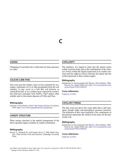
Chemical imaging in Agriculture can perform qualitative 

and quantitative analysis of the ingredient distribution 

(Figure 1), use the science of sampling, set error limits, 

validate and verify results through calibration and standardization, 

create new ways to make measurements 

based on differential spectroscopy properties, and interpret 

data in proper context and communicate results 

(Salzer et al., 2000). Finally, the goal for chemical imaging 

in agro-environment is to recognize and understand chemical 

structures and processes, and to use that knowledge to 

control, classify, or eventually create biological structures 

on demand. Our ability to domesticate crops and eliminate 

the need for hunting and gathering that allowed for the 

establishment of permanent settlements and the development 

of technologically advanced societies has led to 

a greater overall availability of food, both animal and plant. 

Chemical imaging together with biotechnology 

(Schmidt et al., 2009) is a source of great promise for innovations 

ranging from improving the diagnosis and treatment 

of hereditary diseases, to safer drugs, to more 

environmentally friendly herbicides and pesticides to 

microbial processes to clean up the environment (Gowen 

et al., 2007). Making these promises a reality requires 

rethinking some fundamental assumptions. 

Conclusions 

In general, all chemical imaging in Agriculture could benefit 

from the development of higher data acquisition 

speeds, better data storage and management, new chemical 

probes and markers, ultrafast optical detectors, possibility 

of measuring multiple dimensions in parallel and further 

miniaturisation of instrumentation. As chemical imaging 

involves the use of a relatively new analytical technique 

and high cost of instrumentation, the full potential of 

chemical imaging in Agriculture cannot yet be fully realized, 

and that potential, should such analytical techniques 

be implemented on a large scale for the control of intensive 

agricultural and food production, may bring enormous 

benefits for health and prophylactic interventions. 

Chemical Imaging in Agriculture, Figure 1 Classification of 

carrot roots by visual images of transversely cut roots and their 

Raman maps colored according to the band intensity related to 

b-carotene content. (Modified figure of Baranska et al., 2006.) 


Baranska, M., Baranski, R., Schulz, H., and Nothnagel, T., 2006. 

Tissue-specific accumulation of carotenoids in carrot roots. 

Planta, 224, 1028–1037. 

Burrell, M. M., Earnshaw, C. J., and Clench, M. R., 2007. Imaging 

Matrix Assisted Laser Desorption Ionization Mass Spectrometry: 

a technique to map plant metabolites within tissues at 

high spatial resolution. Journal of Experimental Botany, 58, 

757–763.

116 CHEMICAL TIME BOMB, RELATION TO SOIL PHYSICAL CONDITIONS 

Cha, S., Zhang, H., Ilarslan, H. I., Wurtele, E. S., Brachova, L., 

Nikolau, B. J., and Yeung, E. S., 2008. Direct profiling and imaging 

of plant metabolites in intact tissues by using colloidal graphite-assisted 

laser desorption ionization mass spectrometry. The 

Plant Journal, 55, 348–360. 

Ding, S.-Y., Xu, Q., Crowley, M., Zeng, Y., Nimlos, M., Lamed, R., 

Bayer, E. A., and Himmel, 2008. A biophysical perspective on 

the cellulosome: new opportunities for biomass conversion. Current 

Opinion in Biotechnology, 19, 218–227. 

Francis, F. J., 1995. Quality as influenced by color. Food Quality 

and Preference, 6, 149–155. 

Gierlinger, N., and Schwanninger, M., 2007. Review – The potential 

of Raman microscopy and Raman imaging in plant research. 

Spectroscopy, 21, 69–89. 

Glidewell, S. M., 2006. NMR imaging of developing barley grains. 

Journal of Cereal Science, 43, 70–78. 

Gowen, A. A., O’Donnell, C. P., Cullen, P. J., Downey, G., and 

Frias, J. M., 2007. Hyperspectral imaging an emerging process 

analytical tool for food quality and safety control. Trends in Food 

Science and Technology, 18, 590–598. 

Hake, H., Ben-Zur, R., Schechter, I., and Anders, A., 2007. Fast 

optical assessment of pesticide coverage on plants. Analytica 

Chimica Acta, 596, 1–8. 

Himmelsbach, D. S., Barton, F. E., McClung, A. M., and 

Champagne, E. T., 2001. Protein and apparent amylose contents 

of milled rice by NIR-FT/Raman spectroscopy. Cereal Chemistry, 

78, 488–492. 

Jackson, N. B., Chaurand, P. R., Fulghum, J. E., Hernandez, R., 

Higgins, D. A., Hwang, R., Kneipp, K., Koretsky, A. P., 

Larabell, C. A., Stranick, S. J., et al., 2006. Visualizing Chemistry: 

The Progress and Promise of Advanced Chemical Imaging. 

Washington, DC: National Academies Press. 

Lai, A., Santangelo, E., Soressi, G. P., and Fantoni, R., 2007. Analysis 

of the main secondary metabolites produced in tomato 

(Lycopersicon esculentum, Mill.) epicarp tissue during fruit ripening 

using fluorescence techniques. Postharvest Biology and 

Technology, 43, 335–342. 

Lambert, J., Lampen, P., von Bohlen, A., and Hergenröder, R., 

2006. Two- and three-dimensional mapping of the iron distribution 

in the apoplastic fluid of plant leaf tissue by means of magnetic 

resonance imaging. Analytical and Bioanalytical 

Chemistry, 384, 231–236. 

Lichtenthaler, H. K., and Babani, F., 2000. Detection of photosynthetic 

activity and water stress by imaging the red chlorophyll 

fluorescence. Plant Physiology and Biochemistry, 38, 

889–895. 

Mangabeira, P. A., Gavrilov, K. L., de Almeida, A.-A. F., Oliveira, 

A. H., Severo, M. I., Rosa, T. S., da Costa Silva, D., Labejof, L., 

Escaig, F., Levi-Setti, R., Mielke, M. S., Loustalot, F. G., and 

Galle, P., 2006. Chromium localization in plant tissues of 

Lycopersicum esculentum Mill using ICP-MS and ion microscopy 

(SIMS). Applied Surface Science, 252, 3488–3501. 

Perkinsa, M. C., Bell, G., Briggsa, D., Daviesa, M. C., Friedmanb, A., 

Hartb, C. A., Roberts, C. J., and Ruttena, F. J. M., 2008. The 

application of ToF-SIMS to the analysis of herbicide formulation 

penetration into and through leaf cuticles. Colloids and Surfaces. 

B: Biointerfaces, 67, 1–13. 

Roos, W., 2000. Review – Ion mapping in plant cells – methods and 

applications in signal transduction research. Planta, 210, 

347–370. 

Salzer, R., Steiner, G., Mantsch, H. H., Mansfield, J., and Lewis, 

E. N., 2000. Infrared and Raman imaging of biological and biomimetic 

samples. Fresenius’ Journal of Analytical Chemistry, 

366, 712–726. 

Schmidt, M., Schwartzberg, A. M., Perera, P. N., Weber-Bargioni, A., 

Carroll, A., Sarkar, P., Bosneaga, E., Urban, J. J., Song, J., 

Balakshin, M. Y., Capanema, E. A., Auer, M., Adams, P. D., 

Chiang, V. L., and James Schuck, P., 2009. Label-free in situ 

imaging of lignifcation in the cell wall of low lignin transgenic 

Populus trichocarpa. Planta, 230, 589–597. 

Thygesen, L. G., Lokke, M. M., Micklander, E., and Engelsen, 

S. B., 2003. Vibrational microspectroscopy of food. Raman vs. 

FT-IR. Trends in Food Science and Technology, 14, 50–57. 

Xiao, Y., Kreber, B., and Breuil, C., 1999. Localisation of fungal 

hyphae in wood using immunofluorescence labelling and confocal 

laser scanning microscopy. International Biodeterioration 

and Biodegradation, 44, 185–190. 


Anisotropy of Soil Physical Properties 

Biotechnology, Physical and Chemical Aspects 


Isotropy and Anisotropy in Agricultural Products and Foods 

Mapping of Soil Physical Properties 

Plant Disease Symptoms, Identification from Colored Images 

Spatial Variability of Soil Physical Properties 

Surface Properties and Related Phenomena in Soils and Plants 

X-Ray Method to Evaluate Grain Quality 

CHEMICAL TIME BOMB, RELATION TO SOIL 

PHYSICAL CONDITIONS 

Halina Smal 

Institute of Soil Science and Environment Management, 

University of Life Sciences, Lublin, Poland 

Definition 

Chemical time bomb (CTB), originally formulated by 

Stigliani in the late 1980s is defined as 

an unforeseen chain of events resulting in the delayed and 

sudden occurrence of harmful effects due to the mobilization 

or chemical transformation of chemicals stored in soils and 

sediments in response to saturation or alteration in certain 

environmental conditions. (Stigliani, 2002, 99) 

The CTB concept refers to the following: (1) soil/sediment 

ability to store and immobilize toxic chemicals 

(e.g., heavy metals such as Cd, Cu, Pb, and Ni; persistent 

organic compounds such as PCBs - polychlorinated 

biphenyls widely used in the past in many products 

mainly in electrical equipment, and some pesticides like 

DDT- dichloro-diphenyl-trichloroethane) in “chemical 

sinks” having limited capacity, (2) that harmful effects 

of pollution may not be observed directly but long after 

(e.g., decades) loading of the chemical to the environment 

(hence, CTB term). CTB may emerge when a retained, 

inert chemical is mobilized and released because the 

capacity of the sink is either exceeded by an excess of 

the chemical input, or diminished due to changes in 

“capacity-controlling properties” (CCPs), that determine 

the sink storage capacity. In the long term, CCPs are not 

constant and vary as affected by environmental changes 

(e.g., in land use and climate, hydrology). When any of 

CCPs passes a threshold, the system may reverse the role 

from a sink into a source of the chemical, for example, in

CLAY MINERALS AND ORGANO-MINERAL ASSOCIATES 117 

crops and vegetation, ground and surface waters. Such 

a reversal is usually unpredictable, unexpected and sudden 

(the “explosion”) – on a timescale that is relatively 

short in comparison with the time between the initial 

accumulation and the manifestation of detrimental 

effects. 

With respect to heavy metals, particularly important 

soil CCPs are the following: cation exchange capacity 

(CEC), pH, redox potential (Eh), organic matter content, 

salinity, and microbial activity. They are interdependent 

and directly or indirectly related to the soil physical 

conditions; in case of CEC and Eh to the following: 

CEC – soils with a low value have low capacities to retain 

heavy metals by sorption. It depends on clay minerals 

and organic matter content (decreasing reduces CEC) 

and is reflected in soil texture (clay fraction content). 

Eh – decreasing (more reducing conditions) dissolves iron 

and manganese oxides, which mobilizes oxide-sorbed 

toxic chemicals. Its increasing (more oxidizing conditions) 

mobilizes heavy metals by dissolving insoluble 

metal sulfides. Eh is directly influenced by soil moisture 

and may be changed by flooding (Eh decreasing) or 

drainage (Eh increasing) of lands. 

In CTB phenomena, also important are soil physical properties 

influencing leaching and transport of chemicals – water 

retention and water flow, erosion. 

Water flow – depends on soil hydraulic properties. 

Among them, a hydraulic conductivity, which is a measure 

of the ability of a soil to transmit water and 

dissolved solutes and is strongly related to soil texture, 

structure, and water content. 

Soil erodibility – erosion increases the risk of runoff and 

concentrations of toxic substances at locations where 

transported material is deposited. It reflects among 

other properties, soil texture, structure, moisture, and 

organic matter content. It is related to farming activities 

that influence these properties and to changes in land 

use (e.g., it increases with deforestation). 

CTBs example – draining of wetlands in a coastal area of 

Sweden in the 1900s and in the 1940s, resulting in oxidation 

of sulfides to H 2 SO 4 and strong acidification of 

nearby lakes; the Minamata (Japan) catastrophe (for 

details and more examples see Stigliani, 2002). 


Salomons, W., and Stigliani, W. M. (eds.), 1995. Biogeodynamics of 

pollutants in soil and sediments, risk assessment of delayed and 

non-linear responses. Springer: Berlin Heidelberg. 352 pp. 

Stigliani, W. M., 1988. Changes in valued capacities of soils and 

sediments as indicators of nonlinear and time-delayed environmental 

effects. Environmental Monitoring and Assessment, 10, 

245–307. 

Stigliani, W. M., 2002. Contaminated lands and sediments: chemical 

time bombs In Douglas, I. (ed.), Causes and Consequences 

of Global Environmental Change, Vol. 3. In Munn, T. (edin-chief 

), Encyclopedia of Global Environmental Change. 

Chichester/New York: Wiley, pp. 98–115. 

CHISEL 

An edge tool with a flat steel blade with a cutting edge 

used in soil chiselling (loosening by chisel implements). 

CLAY MINERALS AND ORGANO-MINERAL 

ASSOCIATES 

Tatiana Victorovna Alekseeva 

Laboratory Geochemistry and Soil Mineralogy, Institute 

of Physicochemical and Biological Problems of Soil 

Science, Russian Academy of Sciences, Pushchino, 

Moscow region, Russia 

Synonyms 

Phyllosilicates 

Definition 

Clay minerals belong to the family of hydrous aluminum 

phyllosilicates. They make up the fine-grained fraction 

of rocks, sediments, and soils. 

Introduction 

Clay minerals are the most important constituents of 

so-called clay-size fraction (particles are less than 2 micrometers 

[mm] in equivalent spherical diameter) of soils. 

Commonly referred to as “fine-grained,” “submicron,” or 

“ultrafine” particles, recently the term “soil nanoparticles” 

is coming into usage. The clay size fraction in soils is seldom 

composed of a single mineral. Typically, it includes 

mixtures of phyllosilicates, oxides, and hydroxides of Fe, 

Al, and Mn, occasionally quartz and feldspars and organic 

materials – humic substances, enzymes, viruses, etc. 

(Theng and Yuan, 2008) (see Nanomaterials in Soil and 

Food Analysis). Soils’ clay fractions are typically enriched 

in organic C and P, total N, S, and P, inorganic P, Al, Fe, Ca, 

Mg; they have higher cation exchange capacity (CEC) 

in a comparison with bulk soils and coarser fractions. Many 

soils’ basic physical and chemical characteristics: buffer 

capacity, bulk density, cracking and creeping, flocculation 

and dispersion phenomena, hydrophobicity, infiltration, 

shrinkage and swelling phenomena, soil aggregation (see 

Soil Aggregates, Structure, and Stability), soil structure 

and compaction limits, and surface properties (see Adsorption 

Energy and Surface Heterogeneity in Soils, Specific 

Surface Area of Soils and Plants) (see, e.g., Alekseeva 

et al., 1999) are influenced by molecular-scale differences 

in soil clay minerals and/or their concentrations. 

Phyllosilicate minerals in soils 

The structures of phyllosilicates basically consist of sheets of 

SiO 4 tetrahedra and sheets of Al or Mg octahedra (as in 

gibbsite and brucite). Common tetrahedral cations are Si 4+ , 

Al 3+ ,andFe 3+ . Octahedral cations are usually Al 3+ ,Fe 3+ ,

118 CLAY MINERALS AND ORGANO-MINERAL ASSOCIATES 

a 

1:1 layer 

2:1 layer 

[Si 2 Ob 3 Oa 2 ] 

[R 2 

3+ (OH)4 Oa 2 ] or [R 3 

2+ (OH)4 Oa 2 ] 

0.7 nm 

Dioctahedral 1:1 layer R 2 

3+ Si2 O 5 (OH) 4 

Trioctahedral 1:1 layer R 3 

2+ Si2 O 5 (OH) 4 

0.9 nm 

[Si 2 Ob 3 Oa 2 ] 

2:1 layer + hydrated interlayer cations 

d 

[M + x+y–z]xnH 2 O 

[Si 2-x Al x Ob 3 Oa 2 ] 

2+ 

1+ 

3+ [R 3–y R y (OH)2 Oa 4 ] 

2+ 

3+ 

[R 3–z R z (OH)2 Oa 4 ] 

2+ 

[R 2–y R y (OH)2 Oa 4 ] or 

[Si 2-x Al x Ob 3 Oa 2 ] 

Dioctahedral smectite 

(M + x+y x nH 2 O)(R 3+ 

2–y R 2+ 

y )(Si4–x Al x )O 10 (OH) 2 

Trioctahedral smectite 

(M + x+y–z x nH 2 O)(R 2+ 

3–y-z R y 1+ 3+ 

R z )(Si4–x Al x )O 10 (OH) 2 

[R 2 

3+ (OH)2 Oa 4 ] or [R 3 

2+ (OH)2 Oa 4 ] 

[Si 2 Ob 3 Oa 2 ] 

3+ 

Dioctahedral 2:1 layer R 2 Si4 O 10 (OH) 2 

b 

2+ 

Trioctahedral 2:1 layer R 3 Si4 O 10 (OH) 2 

2:1 layer + interlayer cations 

R 1+ 

≅ 1 nm 

≡1.5 nm 

2:1 layer + octahedrally coordinated 

cations in the inerlayer [Si 2 Ob 3 Oa 2 ] 

2+ 3+ 

[R 3 (OH)2 Oa 4 ] or [R 2 (OH)2 Oa 4 ] 

[Si 2 Ob 3 Oa 2 ] 

(R 2+ ,R 3+ ) 3 (OH) 6 

≡1.4 nm 

Trioctahedral or dioctahedral chlorite 

e 

R 2+ 

(R 2+ ,R 3+ ) 3 (Si 4–x Al x )O 10 (OH) 2 (R 2+ ,R 3+ ) 3 (OH) 6 

[Si 1.5 Al 0.5 Ob 3 Oa 2 ] 

[SiAIOb 3 Oa 2 ] 

3+ 2+ 3+ 2+ 

[R 2 (OH)2 Oa 4 ] or [R 3 (OH)2 Oa 4 ] 

[R 2 (OH)2 Oa 4 ] or [R 3 (OH)2 Oa 4 ] 

[Si 1.5 Al 0.5 Ob 3 Oa 2 ] 

[SiAIOb 3 Oa 2 ] 

c 

Dioctahedral true micas 

Dioctahedral brittle micas 

R 1+ 2+ 

AISi 3 R 3 O10 (OH) 2 

R 2+ 3+ 

AI 2 Si 2 R 2 O10 (OH) 2 

Trioctahedral true micas 

Trioctahedral brittle micas 

R 1+ 2+ 

AISi 3 R 3 O10 (OH) 2 R 2+ 2+ 

AI 2 Si 2 R 3 O10 (OH) 2 

Clay Minerals and Organo-Mineral Associates, Figure 1 Different layer structures: (a) 1:1 layer (i.e., kaolinite- and serpentine-like layer), (b) 2:1 layer (i.e., pyrophillite- and 

talc-like layer), (c) 2:1 layer with anhydrous interlayer cations (i.e., the mica-like layer), (d) 2:1 layer with hydrated interlayer cations (i.e., smectite- and vermiculite-like 

layer), (e) 2:1 layer with octahedrally coordinated interlayer cations (i.e., chlorite-like layer). (After Brigatti et al., 2006. With permission from Elsevier.)


Mg 2+ ,andFe 2+ . Octahedra show two different topologies 

related to OH-groups position, i.e., the cis- and the transorientation. 

The 1:1 layer structure consists of the repetition 

of one tetrahedral and one octahedral sheet, and examples 

would be kaolinite and serpentine (Figure 1). 

A 2:1 layer structure consists of an octahedral sheet 

sandwiched between two tetrahedral sheets, and examples 

are micas, smectites, vermiculites, and chlorites. In the 1:1 

layer structure, the unit cell includes six octahedral sites 

(i.e., four cis- and two trans-oriented octahedral) and 

four tetrahedral sites. Six octahedral sites and eight tetrahedral 

sites characterize the 2:1 layer unit cell. Structures 

with all the six octahedral sites occupied are known 

as trioctahedral. If only four of the six octahedra are 

occupied, the structure is referred to as dioctahedral. 

Depending on the composition of the tetrahedral and octahedral 

sheets, the layer will have no charge or will have 

a net negative charge. If the layers are charged, this charge 

is balanced by interlayer cations (Na + ,K + , or others). In 

each case, the interlayer can also contain water. The crystal 

structure is formed from a stack of layers interspaced 

with the interlayers. The periodicity along the c-axis varies 

from 0.91 to 0.95 nm in talc and pyrophyllite to 1.40– 

1.45 nm in chlorite. In talc, the interlayer space is empty, 

whereas in mica and illite it is occupied by anhydrous 

alkaline and alkaline-earth cations (layer periodicity about 

1 nm). The interlayer space of smectite and vermiculite 

contains alkaline or alkaline-earth cations together with 

water molecules (layer periodicity is about 1.2 nm when 

the interlayer position is occupied by cations with lowfield 

strength and water molecules, about 1.5 nm when 

the interlayer is occupied by high-field strength cations 

and water molecules, and more than 1.5 nm when water 

molecules are exchanged by different polar molecules) 

(Brigatti et al., 2006, p. 21). Table 1 gives the classification 

scheme for phyllosilicates with typical layer 

structures and some basic properties (for detail reading 

see also Dixon and Weed, 1989). 

Additionally to these main groups, chain minerals – 

palygorskite (attapulgite) and sepiolite are considered 2:1 

phyllosilicates and these are important constituents in soils 

of arid and semiarid climates. They contain a continuous 

two-dimensional tetrahedral sheet; however, they differ 

from other layer silicates in that they lack continuous octahedral 

sheets. Thus, the structures consist of ribbons of 

2:1 sheets 4 or 6 SiO 4 tetrahedra (in palygorskite and sepiolite, 

respectively) wide connected in a “net” structure with 

holes, which contain a variable amount of zeolitic water. 

Sepiolite is trioctahedral, whereas palygorskite is intermediate 

between di- and trioctahedral. Chain phyllosilicates 

have a fibrous habit with channels running parallel to the 

fiber length. Fiber sizes vary widely but generally range 

from about 10 to about 30 nm in width, and from about 

5 to about 10 nm in thickness. The CEC of these minerals 

is low – 3–20 meq 100 g 1 .Atthesametime,anion 

exchange capacity exceeds 70 meq 100 g 1 which together 

with large external surface (up to 200 m 2 g 1 ) and 

even larger internal pore surface (up to 600 m 2 g 1 ) provides 

high adsorption capacity for cations, anions, and 

neutral molecules, and good suspending or gelling 

characteristics (Mackenzie, 1975; Raussell-Colom and 

Serratosa, 1987; Brigatti et al., 2006). 

Besides monomineralic clay samples and mixtures of 

discreet clay minerals, one more type of mixtures exists – 

interstratified or mixed layer minerals or structures. Mixed 

layers are usually built up by layers of two mineral types 

but may be the combination of more different components. 

Interstratified clay minerals can have ordered or regular 

mixed-layer structures if different layers alternate along 

the c-direction in a periodic pattern (e.g., the stacking of 

A and type B layers can be ABABAB or AABAAB etc.) 

or disordered (irregular) mixed-layer structures, if the 

Clay Minerals and Organo-Mineral Associates, Table 1 Classification scheme for phyllosilicates with typical layer structures 

and their major properties. (Modified after Thorez, 1976.) 

Layer type 

Interlayer 

Net layer charge per 

formula unit (x) 

CEC (meq 

100 g 1 ) 

SSA 

(m 2 g 1 ) Group names 

Subgroups names 

(octahedral layer) 

1:1 Without x 0 3–15 5–40 Kaolinite-serpentine 

(Kandites) 

Di: Kaolinites 

Tri: Serpentines 

2:1 Without x 0 Up to 5 Up to 5 Pyrophyllite-talc Di: Pyrophillites 

Tri: Talcs 

Exchangeable cations, 

anions, molecules, etc. 

x 0.2–0.6 80–120 40–800 Smectites Di: 

Montmorillonites 

Tri: Saponites 

Dry or hydrates cations x 0.6–0.9 100–150 100–400 Vermiculites Di: Vermiculites 

Tri: Vermiculites 

x 0.6–2 10–40 10–100 Micas and illites Di: Muscovites 

Tri: Biotites 

Hydroxide layers x variable 10–40 10–55 Chlorites Di: Sudoites 

Di-Tri: Donbassite 

Tri: Chlorites

120 CLAY MINERALS AND ORGANO-MINERAL ASSOCIATES 

stacking along the c-direction of type A and B layers is random 

(e.g., ABBABAA or AAABABBAAAAABABA 

etc.). Regular sequences are identified by special names. 

For example, the name “rectorite” is attributed to a regular 

interstratification of dioctahedral mica and dioctahedral 

smectite; “tosudite” is a regular interstratification of 

dioctahedral chlorite and dioctahedral smectite. 

Interstratified minerals have been mostly recognized in soils 

but also in sediments and as the hydrothermal and 

weathering products (MacEwan and Ruiz-Amil, 1975; 

Thorez, 1976; Brigatti et al., 2006,p.25). 

Three models of origin of soil clay minerals are: 

(1) inheritance directly from parent materials, (2) transformation 

when the original structure is usually retained 

but the interlayer region is visibly altered, and 

(3) neoformation by the synthesis from the dissolved and 

amorphous products of weathering; here, the structures 

may have no relationship to those of the parent material. 

The soil clay mineral predominance is correlated with climate 

factors (temperature and water availability in the 

soil), because these factors strongly affect the chemical 

weathering in the soil profile. The correlation of soil clay 

mineralogy with climate conditions has been reviewed 

extensively. It was suggested that clay mineralogy follows 

a weathering pattern, from hot and humid to cool and dry, 

in the order kaolinite!smectite!vermiculite!chlorite 

and mixed-layer phyllosilicates!Illite and mica (for 

details see Dixon and Weed, 1989; Wilson, 1999). 

Previously neoformation of clays regarded mostly as 

abiotic processes. Recent findings show that different clay 

minerals can be synthesized with the participation of 

microorganisms (Tazaki, 2006). Konhauser and Urrutia 

(1999) concluded that bacterial clay authigenesis is 

a common biogeochemical process. Like a biomineralization 

process, biochemical weathering of clays also meets 

more interest (Robert and Berthelin, 1986). 

Clay minerals are ultrafine particles and their characterization 

requires special analytical techniques. Standard set 

includes x-ray diffraction, various spectroscopic methods 

such as Mossbauer spectroscopy, infrared spectroscopy, 

NMR spectroscopy, thermal analysis, and electron 

microscopy (for detail reading see Thorez, 1976; Bergaya 

et al., 2006). 

Organo-mineral associates in soils 

In temperate cultivated soils 50–75% of soil organic matter 

(OM) exists within clay-sized organo-mineral particles 

(Kleber et al., 2007). The interactions of clay minerals and 

OM play the important role in the formation and stabilization 

of soil aggregates and the behavior of nutrients and 

pollutants (Six et al., 2002; Alekseeva et al., 2006; 

Besse-Hoggan et al., 2009). 

The ability of minerals to preserve OM results from the 

combined influence of reactive surface sites and a large 

specific surface area (SSA). These properties result from 

heterogeneity and imperfection of the natural mineral 

surfaces and small size of clays and soil oxides (Kogel- 

Knabner et al., 2008). 

The interactions of humic substances with soil clay 

minerals may have a variety of mechanisms which mainly 

depends upon the nature and properties of the organic species, 

the properties of the clay mineral and the kind of 

exchangeable cation at the clay surface, the water content 

of the system, and the pH of the surrounding medium. The 

type of clay becomes increasingly important when the soil 

OM content is low (Cornejo and Harmosin, 1996). 

The interactions of OM with mineral surfaces 

(phyllosilicates and Fe-, Al-, Mn-oxides) and metal ions 

is one of the mechanisms of OM stabilization. Evidence 

comes from the fact that soil OM in fine silt and clay fractions 

is older or has a longer turnover time than OM in 

other soil OM fractions. Adsorption of OM to mineral surfaces 

effects the OM decomposition mechanisms and 

rates. Main chemical mechanisms of interactions are: 

(1) ligand exchange, (2) polyvalent cation bridges, 

(3) weak interactions such as hydrophobic interactions, 

van der Waals forces, and H-bonding (Mineral Organic 

Microbial Interactions) (Luetzow et al., 2006). 

OM bound to minerals mainly by ligand exchange is 

more resistant against mineralization than OM held by 

van der Waals forces. Ca-bridges enhanced the stability 

of sorbed OM but less than by the binding via ligand 

exchange (Kogel-Knabner et al., 2008). 

For each mechanism, only certain amount of OM can 

be protected and each soil has its own protective capacity. 

The mineralogy of soil particles controls the protection of 

OM via the effect of the type and density of active sites 

capable of adsorbing organic materials. The presence of 

Fe-Al oxides – hydroxides increases the surface charge 

density which increases the reactivity of mineral surfaces. 

Kleber et al. (2007) showed that singly coordinated, reactive 

OH groups on Fe and Al oxides and at edge sites of 

phyllosilicates, which are able to form strong bonds by 

ligand exchange, are a measure of the amount of OM stabilized 

in soils in organo-mineral associations. 

Preferential binding at reactive sorption sites favors 

typically discontinuous surface accumulation of OM 

rather than in a continuous coating. Thus, OM is not distributed 

over the available mineral surfaces but clustered 

(Clusters in Soils) in small patches with some vertical 

extension (Kaiser and Guggenberger, 2003; Kleber et al., 

2007). Recently, Kleber et al. (2007) came to the conclusion 

that adsorbed OM creates the zonal organo-mineral 

architecture with regular features: contact zone, hydrophobic 

zone, and kinetic zone. The molecules of the inner 

zone are the most stable, and molecules of the outer zone 

have the faster exchange with soil solution. It is suggested 

that proteins (N-containing materials) play a prominent 

role in the formation of organo-mineral complexes due 

to both the relatively high abundances of these compounds 

in soils and the ability of these materials to adsorb irreversibly 

to mineral surfaces. Proteins can bind particularly 

strongly and create a basal layer with further opportunities 

for more numerous interactions. The affinity of proteins


for all types of interfaces found in soils originates in the 

flexibility of the polypeptide chain and in the diversity 

of the 2-amino acids that can be classified as positively, 

neutrally, or negatively charged and on a hydrophobic 

scale from polar (hydrophilic) to non-polar (Quiquampoix 

and Burns, 2007). 

Additionally to chemical stabilization of OM in soils, 

its physical protection in soil microaggregates influences 

OM accumulation (Physical Protection of Organic Carbon 

in Soil Aggregates). 

Summary 

Interactions of clay minerals with OM (soil natural organic 

polymers) modify properties of both partners and have the 

large-scale effect on the physical, chemical, and biological 

properties of soils. Fractionation of soil organic substances 

due to the properties of a mineral matrix is the 

other aspect of these interactions. Up to now limited information 

is available on the relationships between mineralogy 

and the chemistry of bound OM. Solid state NMR 

spectroscopy ( 13 C, 15 N, 31 P, 1 H, etc.) is a promising tool 

for solving this problem. Kogel-Knabner et al. (2008) 

showed that mineral-bound OM is depleted in lignin and 

phenolic components. Clay fractions generally show 

a higher content alkyl-C groups than whole soils and 

higher proportions of carboxyl-C than plant residues, 

indicative of the more oxidized stage of the stabilized 

OM. Laird et al. (2001) postulated that existing relationships 

between clay mineralogy and the chemical nature 

of the associated humic substances indicate that either soil 

clay mineralogy strongly influences the humification process 

or that humic substances with different properties are 

selectively adsorbed on different clay mineral species. 

Further investigations of the OM associated with different 

clay minerals are needed before the role of clay–organic 

interactions on OM constitution, stabilization and turnover 

times, diagenetic transformations, and other aspects 

will be clear. 


Alekseeva, T. V., Alekseev, A. O., Sokolowska, Z., and Hajnos, M., 

1999. Relationship between mineralogical composition and 

physical properties of soils. Eurasian Soil Science, 32, 548–557. 

Alekseeva, T., Besse, P., Binet, F., Delort, A. M., Forano, C., 

Josselin, N., Sancelme, M., and Tixier, C., 2006. Effect of earthworm 

activity (Aporrectodea giardi) on atrazine adsorption and 

biodegradation. European Journal of Soil Science, 57, 295–307. 

Bergaya, F., Theng, B. K. G., and Lagaly, G. (eds.), 2006. Handbook 

of Clay Science. Amsterdam: Elsevier. 

Besse-Hoggan, P., Alekseeva, T., Sancelme, M., Delort, A. M., and 

Forano, C., 2009. Atrazine biodegradation modulated by clays 

and clay/humic acid complexes. Environment Pollution, 157, 

2837–2844. 

Brigatti, M. F., Galan, E., and Theng, B. K. G., 2006. Structures and 

Mineralogy of Clay Minerals. In Bergaya, F., Theng, B. K. G., 

and Lagaly, G. (eds.), Handbook of Clay Science. Amsterdam: 

Elsevier. 

Cornejo, J., and Harmosin, M. C., 1996. Interactions of humic substances 

and soil clays. In Piccolo, A. (ed.), Humic Substances in 

Terrestrial Ecosystems. Amsterdam: Elsevier, pp. 595–624. 

Dixon, J. B., and Weed, S. B. (eds.), 1989. Minerals in Soil Environments, 

2nd edn. Madison: Soil Science Society of America. 

SSSA Book Series 1. 

Kaiser, K., and Guggenberger, G., 2003. Mineral surfaces and soil 

organic matter. European Journal of Soil Science, 54, 219–236. 

Kleber, M., Sollins, P., and Sutton, R., 2007. A conceptual model of 

organo-mineral interactions in soils: self-assembly of organic 

molecules fragments into zonal structures on mineral surfaces. 

Biogeochemistry, 85, 9–24. 

Kogel-Knabner, I., Guggenberger, G., Kleber, M., Kandeler, E., 

Kalbitz, K., Scheu, S., Eusterhues, K., and Leinweber, P., 

2008. Organo-mineral associations in temperate soils: integrating 

biology, mineralogy, and organic matter chemistry. Journal 

of Plant Nutrition and Soil Science, 171, 61–82. 

Konhauser, K. O., and Urrutia, M. M., 1999. Bacterial clay 

authigenesis: a common biogeochemical process. Chemical 

Geology, 161, 399–413. 

Laird, D. A., Martens, D. A., and Kingery, W. L., 2001. Nature of 

clay-humic complexes in an agricultural soil: I. chemical, biochemical, 

and spectroscopic analyses. Soil Science Society of 


Luetzow, M. V., Kogel-Knabner, I., Ekschmitt, K., Matzner, E., 

Guggenberger, G., Marshner, B., and Flessa, H., 2006. Stabilization 

of organic matter in temperate soils: mechanisms and their 

relevance under different soil conditions – a review. European 

Journal of Soil Science, 57, 426–445. 

MacEwan, D. M. C., and Ruiz-Amil, A., 1975. Interstratified Clay 

Minerals. In Gieseking, J. E. (ed.), Inorganic Components, Soil 

components. New york: Springer, Vol. 2, pp. 267–334. 

Mackenzie, R. C., 1975. The classification of soil silicates and 

oxides. In Gieseking, J. E. (ed.), Soil Components. Vol. 2: Inorganic 

Components. New York: Springer, pp. 1–26. 

Quiquampoix, H., and Burns, R. G., 2007. Interactions between 

proteins and soil mineral surfaces: environmental and health 

consequences. Elements, 3(6), 401–406. 

Raussell-Colom, J. A., and Serratosa, J. M., 1987. Reactions of 

clays with organic substances. In Newman, A. C. D. (ed.), Chemistry 

of Clays and Clay Minerals. London: Longman Scientific 

& Technical, pp. 371–422. Mineralogical Society Monograph 

No. 6. 

Robert, M., and Berthelin, J., 1986. Role of biological and biochemical 

factors in soil mineral weathering. In Huang, P. M., and 

Schnitzer, M. (eds.), Interactions of Soil Minerals with Natural 

Organics and Microbes. Madison: Soil Science Society of 

America, pp. 453–495. SSSA special publication 17. 

Six, J., Conant, R. T., Paul, E. A., and Paustian, K., 2002. Stabilization 

mechanisms of soil organic matter: implications for C-saturation 

of soils. Plant and Soil, 241, 155–176. 

Tazaki, K., 2006. Clays, microorganisms, and biomineralization. In 

Bergaya, F., Theng, B. K. G., and Lagaly, G. (eds.), Handbook of 

Clay Science. Amsterdam: Elsevier, pp. 477–498. 

Theng, B. K. G., and Yuan, G., 2008. Nanoparticles in the Soil Environment. 

Elements, 4, 395–399. 

Thorez, J., 1976. Practical Identification of Clay Minerals. Belgium: 

Liege State University, Institute of Mineralogy. 

Wilson, J. J., 1999. The origin and formation of clay minerals in 

soil; past, present and future perspectives. Clay Minerals, 34, 

7–25. 


Adsorption Energy and Surface Heterogeneity in Soils 

Buffer Capacity of Soils 

Bulk Density of Soils and Impact on Their Hydraulic Properties 

Clusters in Soils 

Compaction of Soil 

Cracking in Soils

122 CLAYPAN AND ITS ENVIRONMENTAL EFFECTS 

Flocculation and Dispersion Phenomena in Soils 

Hydrophobicity of Soil 

Infiltration in Soils 

Nanomaterials in Soil and Food Analysis 


Shrinkage and Swelling Phenomena in Soils 

Soil Aggregates, Structure, and Stability 

Specific Surface Area of Soils and Plants 

CLAYPAN AND ITS ENVIRONMENTAL EFFECTS 

Stephen H. Anderson 

Department of Soil, Environmental, and Atmospheric 

Sciences, University of Missouri, Columbia, MO, USA 

Synonyms 

Argillic horizon; Pseudogley; Stagnic properties 

Definition 

Claypan refers to a subsoil layer, having a much higher 

clay content than the surface horizons. This layer is slowly 

permeable and is separated by a sharply defined boundary 

from overlying horizons. Claypans are dense and hard 

when dry but plastic and sticky when wet. (Soil Science 

Society of America, 2008). These soils often have 

a perched water table present above the claypan during 

a portion of the year. 

Pan. A pan can be genetic or induced. A genetic pan is 

a natural subsurface soil layer with low or very low 

hydraulic conductivity. The layer differs in physical and 

chemical properties from the soil layers immediately 

above and below the pan. Some genetic pans include claypans, 

fragipans, and hardpans. An induced pan is 

a subsurface layer having a higher bulk density and lower 

total porosity than the soil layers immediately above and 

below the pan and is a result of pressure that has been 

applied by normal tillage operations or other artificial 

means. Synonyms for these induced pans include 

plowpans, plowsoles, pressure pans, or traffic pans (Soil 

Science Society of America, 2008). 

Introduction 

Soils with claypans include significant areas throughout 

the world. In the Midwestern USA, these soils are 

included in Major Land Resource Area (MLRA) 113 Central 

Claypan Area (2.9 million hectares), with most soils 

classified as Aqualfs and some Udalfs. The United 

Nations FAO system classifies these soils as Eutric Planosols 

(Food and Agriculture Organization of the United 

Nations, 2001). Eutric Planosols have a global extent of 

47.53 million hectares. Planosols include 130 million 

hectares and are extensive in southern Brazil, northern 

Argentina, Paraguay, eastern Africa, South Africa, eastern 

Australia, eastern United States, and in southeast Asia 

from Bangladesh to Thailand (Food and Agriculture Organization 

of the United Nations, 2001). 

The US Soil Classification System of 1938 used the 

name Planosols for claypan soils. The subsequent US classification 

system, USDA Soil Taxonomy, includes Planosols 

in the Great Groups Albaqualfs, Albaquults, and 

Arialbolls. Claypan soils are in the Great Group 

Albaqualfs. 

Claypan soils include a significant amount of area 

within the Midwestern USA (Blanco-Canqui et al., 

2002). Soils in this area are characterized by a subsoil 

horizon with an abrupt and significant increase in clay 

content within a short vertical distance in the soil profile 

(Soil Science Society of America, 2008). The Midwestern 

US claypan region and similar soils encompass an area of 

about 4 million hectares within Missouri, Illinois, and 

Kansas (Anderson et al., 1990). The depth to the claypan 

varies from 0.10 to 0.50 m with clay content ranging from 

350 to 600 g/kg (35–60%; Blanco-Canqui et al., 2002). 

Dominant clay minerals include smectites with high 

shrink swell potential. 

Throughout the year, these clays swell during the winter 

and spring periods and often shrink during the late 

summer and early autumn periods. When the clays are 

swollen, their low saturated hydraulic conductivity 

impedes infiltration and perches water above the claypan, 

causing a high probability of runoff (Blanco-Canqui et al., 

2002). When the clays shrink, preferential flow through 

these cracks is significant (Baer and Anderson, 1997). 

Most claypan soils are classified in high runoff hydrologic 

groups (Lerch et al., 2008). Soils primarily on 

hillslopes in dissected till have a slow infiltration rate and 

moderate runoff potential due to argillic horizons or 

paleosols that impede downward movement of water. Soils 

occurring at summit landscape positions have a very slow 

infiltration rate and high runoff potential due to claypans. 

Hydrology 

Soil texture and structure have strong effects on saturated 

hydraulic conductivity, K sat (Blanco-Canqui et al., 2002). 

Clay-textured soils typically have low to very low K sat 

values. Due to their low subsoil permeability, claypan 

soils perch water and create lateral flow and surface runoff. 

Field work on claypan hydrology suggests that runoff 

rates may be equal to rainfall under saturated conditions 

(Saxton and Whitaker, 1970). Long-term studies of runoff 

and rainfall with the McCredie rainfall-erosion plots at 

Kingdom City, Missouri, USA indicate that lateral flow 

known as interflow is a significant component of the total 

runoff during springtime when precipitation is usually the 

most intense and erosion rates are highest (Minshall and 

Jamison, 1965; Ghidey and Alberts, 1998). Claypan soils 

have enhanced runoff during winter and spring periods 

due to very low infiltration rates. 

In situ lateral K sat has been estimated for claypan soils 

in monoliths 0.25-m wide by 0.50-m long by 0.23-m deep 

(Blanco-Canqui et al., 2002). Field measurements of lateral 

K sat provided a value of 72 mm h 1 . This value corresponds 

well to soil core (76-mm diameter by 76-mm

CLAYPAN AND ITS ENVIRONMENTAL EFFECTS 123 

length) estimates of 71 mm h 1 through the silt loam surface 

horizon (Figure 1). The field estimate of K sat for the 

claypan was 0.9 mm h 1 . The lowest K sat of the profile 

measured with soil cores was 2 mm h 1 , which occurred 

within the 0.50–0.75-m depth (Figure 1), just below the 

claypan (depth of maximum clay concentration; Blanco- 

Canqui et al., 2002). The physical nature of this layer 

was weakly developed, compact, with a firm structure. 

A high probability of interflow occurs within these soils 

(Jamison et al., 1968; Wilkinson and Blevins, 1999). 

Information on in situ lateral K sat through the horizons 

above the claypan is important for determining their ability 

to conduct water laterally and assessing runoff and erosion. 

Because of their hydrologic attributes, claypan soils 

have quite different effective K sat values with depth from 

other Alfisols. Information on K sat depth distribution is 

valuable in explaining claypan hydrology and for the 

characterization of variability in horizons of low and 

high permeability required for accurate flow studies 

(Blanco-Canqui et al., 2002). 

Depth (m) 

0.001 0.1 10 1000 

0 

0.2 

0.4 

0.6 

0.8 

1 

1.2 

1.4 

1.6 

1.8 

2 

Saturated hydraulic conductivity (min h –1 ) 

Jamison and Peters 

Doll 

McGinty 

Zeng 

Blanco – No bentonite 

Blanco – bentonite 

Baer and Anderson 

95% Confidence interval 

Claypan and its Environmental Effects, Figure 1 Comparison 

of saturated hydraulic conductivity (K sat ) data for claypan soils 

(Blanco-Canqui et al., 2002). Error bars represent 95% confidence 

intervals of mean K sat values (n = 9). Data obtained with 

bentonite (Blanco-Bentonite) to plug visible pores represent K sat 

data for claypan soils. (Reprinted with permission from the Soil 

Science Society of America.) 

Claypan soils under native vegetation have significantly 

different hydraulic properties compared to soils 

under long-term grain crop management (Udawatta 

et al., 2008). Differences can be attributed to better structure 

as well as preserved pore networks. Soils under native 

vegetation have enhanced macropore flow, permanent 

roots, and higher organic matter content. Native permanent 

vegetation prevents water erosion, which increases 

the thickness of surface horizons; eroded soils have about 

0.25 m thinner silt loam surface horizons than soils with 

native vegetation. Thicker surface horizons with coarser 

soil textures have higher hydraulic conductivity values. 

Under long-term grain crop management, soil hydraulic 

properties for claypan soils can significantly change due 

to a reduction in surface layer thickness above the clay 

layer through erosion as well as from the traffic by agricultural 

equipment. Improvements in these properties have 

been observed when using permanent vegetative buffers 

such as cool season grass buffers and agroforestry tree 

buffers (Seobi et al., 2005). Although the claypan horizon 

dominates the surface hydrology for these soils, buffers 

often provide benefits by slightly reducing runoff from 

soils under row crop management. 

Conservation Reserve Program (CRP) and hay management 

systems increased field-measured infiltration 

rates in a summit landscape position compared to grain 

crop systems (Jung et al., 2007). Hydraulic conductivity 

measured in a backslope position for CRP and hay 

cropping systems was 16 and 10 times higher, respectively, 

than for a mulch-tilled grain cropping system (Jiang 

et al., 2007a). This was attributed in part to perennial 

grasses improving aggregate stability and soil organic carbon. 

Backslope landscape positions are more vulnerable 

to soil degradation with grain cropping systems compared 

to other landscape positions. 

Soil erosion and agrichemical runoff 

Due to enhanced runoff on claypan soils, soil erosion and 

sediment transport can be a concern. Minimum tillage as 

well as no-till systems are recommended to reduce this 

problem. Some studies have shown that no-till management 

can slightly enhance runoff on claypan soils relative 

to conventional tillage systems (Ghidey and Alberts, 

1998; Ghidey et al., 2005); however, other studies have 

shown no differences in runoff among tillage systems 

(Lerch et al., 2008). No-till systems with corn (Zea mays) 

and soybean (Glycine max) cropping systems have significantly 

reduced sediment transport. Most annual soil loss 

(80% of annual loss) occurs during the rough fallow and 

seedbed preparation periods, with soil loss under no-till 

management five to seven times lower compared to other 

tillage systems (Ghidey and Alberts, 1998). 

Vegetative filter strips have been used on claypan soils 

to mitigate surface runoff, sediment, and nutrient losses 

(Blanco-Canqui et al., 2004). Narrow, 1-m-long native 

switchgrass (Panicum virgatum) barriers in combination 

with 8-m-long fescue (Festuca arundinacea) filter strips

124 CLAYPAN AND ITS ENVIRONMENTAL EFFECTS 

significantly reduced sediment transport as well as organic 

N, nitrate, ammonium, particulate P, and phosphate runoff 

compared to traditional fescue filter strips. 

These vegetative filter systems have also been shown 

to reduce dissolved and sediment-bound herbicide losses 

in runoff (Lerch et al., 2008). Studies evaluated the 

transport of glyphosate [N-(phosphonomethyl)glycine], 

atrazine [6-chloro-N 2 -ethyl-N 4 -isopropyl-1,3,5-triazine- 

2,4-diamine], and metolachlor [2-chloro-N-(6-ethyl-otolyl)-N-[(1RS)-2-methoxy-1-methylethyl]acetamide]. 

Four 

meters of native vegetation buffers (mostly eastern 

gamagrass [Tripsacum dactyloides] and switchgrass) 

reduced herbicides about 75–80% in runoff. Four meters 

of native species resulted in greater reductions in herbicide 

transport compared to 8 m of fescue. Buffers enhance plant 

transpiration which enhances infiltration to reduce surface 

runoff in these high runoff potential claypan soils. As 

a general pattern, herbicide concentration or mass loss was 

greatest for the first runoff event and decreased rapidly as 

the season progressed. 

Contour buffer strips have been demonstrated to reduce 

runoff, sediment, and nutrient losses in cropped watersheds 

(Udawatta et al., 2002). Paired watersheds were 

used to make an assessment of the degree of benefit from 

these contour buffers. Agroforestry buffers (trees and 

grasses) and contour grass buffers were found to reduce 

runoff (1% and 10%), sediment (0% and 19%), total phosphorus 

(17% and 8%), and nitrate (37% and 24%) losses. 

Most runoff reductions occurred during the second and 

third years after treatment establishment. 

Management of runoff and associated effects on surface 

sediment, nutrient, and herbicide transport is an important 

challenge when using claypan soils for grain crop production. 

No-till management has been shown to enhance herbicide 

runoff relative to conventional tillage systems due 

to lack of herbicide incorporation and slightly increased 

runoff with no-till systems (Ghidey et al., 2005). 

Agrichemical leaching 

The claypan soils of the Midwestern USA contain silt 

loam surface textures and silty clay subsoils (Blanco- 

Canqui et al., 2002). The subsoil contains a high proportion 

of montmorillonitic clay, which results in 

a relatively impermeable soil horizon when wet. Since 

the claypan is highly impermeable, the assumption is often 

made that water and solutes cannot move through the claypan 

to reach groundwater. However, cracks often occur in 

these soils when they are cropped and their water content 

is low (Baer and Anderson, 1997). These cracks can allow 

preferential flow of water and chemicals. In addition, soils 

have natural features such as interpedal planar voids and 

biologically induced, highly conductive macropores, 

which may act as channels for water and chemical transport. 

In one study, claypans were hypothesized to restrict 

the movement of agrichemicals to groundwater; however, 

N fertilizer moved rapidly through preferential flow paths 

in the soil into the underlying glacial till aquifer (Blevins 

et al., 1996; Wilkinson and Blevins, 1999). About one 

third of the N fertilizer migrated to the groundwater, while 

another one third was lost due to denitrification which can 

be a challenge for these soils since they have high soil 

water content in the spring. 

Although enhanced annual runoff occurs from claypan 

soils, vertical transport can occur after periods of 

infrequent precipitation. Kazemi et al. (2008) found 

enhanced herbicide leaching in soils which had antecedent 

water content near the permanent wilting point (dry 

treatment). Atrazine, alachlor [2-chloro-2 0 ,6 0 -diethyl-Nmethoxymethylacetanilide], 

and the bromide tracer were 

detected significantly deeper (0.15–0.30 m) when applied 

to a dry treatment compared to the wet treatment (water 

content near field capacity). Herbicide retardation 

coefficients estimated using soil properties were substantially 

higher compared to estimates from herbicide and 

bromide profile concentrations, suggesting evidence of 

nonequilibrium adsorption of atrazine and alachlor probably 

due to less surface area available for adsorption when 

transport occurs in shrinkage cracks. Preferential flow of 

atrazine and alachlor herbicides was found when applications 

occurred on initially dry claypan soils. The deeper 

movement of herbicides in initially dry plots was attributed 

to the presence of shrinkage cracks resulting from 

low soil water content. 

Herbicide degradation has been found to decrease with 

dry soil water conditions (Kazemi et al., 2008). Degradation 

was found to be lower for initially dry conditions 

compared to initially wet conditions. This was attributed 

to better microbial growth in soils under initially moist 

conditions. Thus, dry claypan soils enhance preferential 

transport of herbicides and also decrease their rate of 

degradation. 

Plant productivity 

Variable claypan properties across the landscape affect 

grain yield due to soil property effects on root growth 

(Myers et al., 2007). Soybean roots were inhibited in 

E horizons above the claypan; however, roots were stimulated 

20–40 cm below the initial claypan depth. Depth to 

claypan can be used to predict soybean root distributions 

in claypan landscapes. The depth to the claypan can be 

rapidly assessed using the apparent bulk electrical conductivity 

measured using electromagnetic induction (Kitchen 

et al., 1999). The topsoil thickness above the claypan layer 

is highly related to the plant available water capacity 

(Jiang et al., 2007b) and the crop yield (Kitchen et al., 

1999). Apparent bulk electrical conductivity from these 

sensors can be correlated with crop yield due to the effect 

of the depth to the high charge claypan layer affecting the 

sensor signal (Kitchen et al., 1999). 

Summary 

Crop productivity is highly sensitive to topsoil thickness 

in claypan soils. Prevention of soil erosion is critical in 

maintaining grain production as well as enhancing water

CLIMATE CHANGE: ENVIRONMENTAL EFFECTS 125 

infiltration in these soils. Conservation best management 

practices (BMPs) are important to reduce and prevent soil 

erosion. In some cases, selection of a BMP for one desired 

outcome may be opposite to another desired outcome 

(e.g., no-till may be good for erosion control but can 

increase herbicide loss). When this is the case, priorities 

will need to be established in order to select the appropriate 

BMP (Lerch et al., 2008). 


Anderson, S. H., Gantzer, C. J., and Brown, J. R., 1990. Soil physical 

properties after 100 years of continuous cultivation. Journal 

of Soil and Water Conservation, 45, 117–121. 

Baer, J. U., and Anderson, S. H., 1997. Landscape effects on desiccation 

cracking in an Aqualf. Soil Science Society of America 

Journal, 61, 1497–1502. 

Blanco-Canqui, H., Gantzer, C. J., Anderson, S. H., Alberts, E. E., 

and Ghidey, F., 2002. Saturated hydraulic conductivity and its 

impact on simulated runoff for claypan soils. Soil Science Society 

of America Journal, 66, 1596–1602. 

Blanco-Canqui, H., Gantzer, C. J., Anderson, S. H., Alberts, E. E., 

and Thompson, A. L., 2004. Grass barrier and vegetative filter 

strip effectiveness in reducing runoff, sediment, nitrogen, and 

phosphorous loss. Soil Science Society of America Journal, 68, 

1670–1678. 

Blevins, D. W., Wilkison, D. H., Kelly, B. P., and Silva, S. R., 1996. 

Movement of nitrate fertilizer to glacial till and runoff from 

a claypan soil. Journal of Environmental Quality, 25, 584–593. 

Food and Agriculture Organization of the United Nations, 2001. 

Lecture notes on the major soils of the world. FAO Corporate 

Document Repository. Available from World Wide Web: http:// 

www.fao.org/DOCREP/003/Y1899E/y1899e12.htm#P158_22451. 

Ghidey, F., and Alberts, E. E., 1998. Runoff and soil losses as 

affected by corn and soybean tillage systems. Journal of Soil 

and Water Conservation, 53, 64–70. 

Ghidey, F., Blanchard, P. E., Lerch, R. N., Kitchen, N. R., Alberts, 

E. E., and Sadler, E. J., 2005. Measurement and simulation of 

herbicide transport from the corn phase of three cropping systems. 

Journal of Soil and Water Conservation, 60, 260–273. 

Jamison, V. C., Smith, D. D., and Thornton, J. F., 1968. Soil and 

Water Research on a Claypan Soil. USDA Technical Bulletin 

1379. Washington: US Government Print Office. 

Jiang, P., Anderson, S. H., Kitchen, N. R., Sadler, E. J., and 

Sudduth, K. A., 2007a. Landscape and conservation management 

effects on hydraulic properties of a claypan-soil 

toposequence. Soil Science Society of America Journal, 71, 

803–811. 

Jiang, P., Anderson, S. H., Kitchen, N. R., Sudduth, K. A., and 

Sadler, E. J., 2007b. Estimating plant-available water capacity 

for claypan landscapes using apparent electrical conductivity. 

Soil Science Society of America Journal, 71, 1902–1908. 

Jung, W. K., Kitchen, N. R., Anderson, S. H., and Sadler, E. J., 

2007. Crop management effects on water infiltration for claypan 

soils. Journal of Soil and Water Conservation, 62, 55–63. 

Kazemi, H. V., Anderson, S. H., Goyne, K. W., and Gantzer, C. J., 

2008. Atrazine and alachlor transport in claypan soils as 

influenced by differential antecedent soil water content. Journal 

of Environmental Quality, 37, 1599–1607. 

Kitchen, N. R., Sudduth, K. A., and Drummond, S. T., 1999. Soil 

electrical conductivity as a crop productivity measure for claypan 

soil. Journal of Production Agricultural, 12, 607–617. 

Lerch, R. N., Sadler, E. J., Kitchen, N. R., Sudduth, K. A., Kremer, 

R. J., Myers, D. B., Baffaut, C., Anderson, S. H., and Lin, C. H., 

2008. Overview of the mark Twain/Salt river basin conservation 

effects assessment project. Journal of Soil and Water Conservation, 

63, 345–359. 

Minshall, N. E., and Jamison, V. C., 1965. Interflow in claypan 

soils. Water Resources Research, 1, 381–390. 

Myers, D. B., Kitchen, N. R., Sudduth, K. A., Sharp, R. E., and 

Miles, R. J., 2007. Soybean root distribution related to claypan 

soil properties and apparent soil electrical conductivity. Crop 

Science, 47, 1498–1509. 

Saxton, K. E., and Whitaker, F. D., 1970. Hydrology of a Claypan 

Watershed. Research Bulletin 974. Columbia: Missouri Agricultural 

Experiment Station. 

Seobi, T., Anderson, S. H., Udawatta, R. P., and Gantzer, C. J., 

2005. Influence of grass and agroforestry buffer strips on soil 

hydraulic properties for an Albaqualf. Soil Science Society of 


Soil Science Society of America, 2008. Glossary of soil science 

terms, 2008 edition. Soil Science Society of America, Madison 

(available online at https://www.soils.org/publications/soilsglossary). 

Udawatta, R. P., Krstansky, J. J., Henderson, G. S., and Garrett, 

H. E., 2002. Agroforestry practices, runoff, and nutrient loss: 

a paired watershed comparison. Journal of Environmental Quality, 

31, 1214–1225. 

Udawatta, R. P., Anderson, S. H., Gantzer, C. J., and Garrett, H. E., 

2008. Influence of prairie restoration on CT-measured soil pore 

characteristics. Journal of Environmental Quality, 37, 219–228. 

Wilkison, D. H., and Blevins, D. W., 1999. Observations on preferential 

flow and horizontal transport of nitrogen fertilizer in 

the unsaturated zone. Journal of Environmental Quality, 28, 

1568–1580. 


Cracking in Soils 

Electrical Resistivity to Assess Soil Properties 

Layered Soils, Water and Solute Transport 


Wetting and Drying, Effect on Soil Physical Properties 

CLEAVAGE PLANE 

The smooth, flat surface along which a mineral (also soil 

clay mineral) readily breaks. 




CLIMATE CHANGE: ENVIRONMENTAL EFFECTS 

Miroslav Kutílek 

Prague, Czech Republic 

Synonyms 

Global warming

126 CLIMATE CHANGE: ENVIRONMENTAL EFFECTS 

Definition 

Climate is defined as the statistical evaluation of meteorological 

data. They are air temperature, humidity, rainfall, 

wind, and eventually other observed elements in a given 

region over a long time period; the World Meteorological 

Organisation recommends 30 years, but longer periods 

may be used depending upon the purpose. The obtained 

results are applied in climate classification; the oldest 

and well known is the Köppen classification. Several other 

classifications are used, too, again according to the purpose. 

Climate should not be confused with weather, which 

is the set of meteorological data valid at time of observation, 

usually on scale of days. 

Recent climate change 

Introduction 

The recent climate change started about 1850. Actually 

the estimation of the year is a matter of general agreement 

and it is not strictly equal to local or regional observations. 

The climate change is usually characterized by the global 

temperature in recent studies; other climate characteristics 

are only sometimes mentioned, too. The temperature 

increase in the twentieth century was estimated as 

0.74 C and the rate of its rise is increasing. Eleven of the 

last 12 years (1995–2006) rank among the 12 warmest 

years in the instrumental record of global surface temperature 

(since 1850). The warmest years in the instrumental 

record of global surface temperatures are 1998 and 2005 

(Trenberth et al., 2007), with 1998 frequently considered 

as the first one in the rank. Measured temperature of the 

global ocean has increased to depths of at least 3,000 m 

in the last 40 years. The energy balance shows that the 

ocean absorbs more than 80% of the heat added to the climate 

system. The global warming caused the rate of rise of 

seawater level by 1.8 0.3 mm/year in the second half of 

the twentieth century (White et al., 2005) (Figure 1). 

The reported rise of the global temperature by 0.74 C 

does not mean that the temperature rose uniformly over 

the Earth. This same value would not have been obtained 

Difference from 1961–1990 

(mm) (C) 

0.5 

0.0 

–0.5 

a 

50 

0 

–50 

–100 

–150 

(million km 2 ) 

b 

4 

0 

–4 

Changes in temperature, sea level and 

northern hemishere snow cover 

Global average temperature 

Global average sea level 

Northern hemisphere snow cover 

14.5 

14.0 

13.5 

40 

36 

32 

Temperature (C) (million km 2 ) 

c 

1850 1900 1950 2000 

Year 

Climate Change: Environmental Effects, Figure 1 Change of the surface global average temperature for the time period 

1850–2007 (top); change of the global seawater level elevation (center); change of the northern hemisphere snow covered area in 

March–April (bottom). Smoothed curves represent decadal averaged values, while circles show yearly values. (According to Fig. SPM-3, 

IPCC, 2007; Summary for Policymakers.)


everywhere that the temperature was measured locally 

during the past 100 years. The observed warming has been 

greater over land than that over the oceans, owing to the 

smaller thermal capacity of the land. Since the continents 

occupy larger area on the northern hemisphere, there was 

a tendency for a higher temperature rise in the northern 

than in the southern hemisphere (Trenberth et al., 2007). 

Values of average temperature rise also differ according 

to differences in climate of various regions. The rise is 

very small in the equatorial regions and increases with 

the latitudes, both north and south. The latitude dependence 

is only one of the many factors that play a role 

and the local average temperature rise depends upon its 

particular geographical position on a continent. Values 

differ for inland climates compared with lands close to 

the ocean. In Central Europe, the average temperature 

increased between 1.1 C and 1.3 C in 100 years (Czech 

Meteorological Institution, 2007), while in Northern 

Ireland at Armagh Observatory the increase was only 

1.2 C in 200 years, that is, from 1796 to 2002. Within 

the Arctic Circle at latitudes between 70 and 90 , the 

average temperature rise was 2.1 C in the period 1880– 

2004 (Trenberth et al., 2007, Figure 3.7). During the first 

60 years of that 124-year period, the average temperature 

increased, then decreased for the next 20 years, and again 

increased for the following 44 years. In that 124-year 

period, the average temperature rises were there higher 

in the period 1920–1940 than they are today. 

Warming is strongest over the continental interiors of Asia 

and northwestern North America and over some mid-latitude 

ocean regions of the southern hemisphere as well as southeastern 

Brazil. In the recent period, some regions have 

warmed substantially while a few have cooled slightly on 

an annual basis. (Trenberth et al., 2007, p. 250) 

These few examples enable us to imagine how difficult 

it is to estimate the global temperature and its rise merely 

from the data obtained from any number or all meteorological 

stations. “No single location follows the global 

average, and the only way to monitor the globe with any 

confidence is to include observations from as many 

diverse places as possible (Trenberth et al., 2007, p. 

250).” The estimation of the global temperature from the 

surface meteorological stations was therefore a difficult 

task. During the last 28 years, the instrumentation in satellites 

was applied to measure the Earth’s global surface 

temperature. These methods of measurement are considered 

by meteorologists to be the most objective proof of 

global warming. It was just by these methods that the 

temperature was found as no more rising in the last 

decade (Solomon et al., 2007; Easterling and Wehner, 

2009). 

Measuring methods 

In 1653, organized measurements of air temperature 

began in northern Italy with the first meteorological network 

initiated in Tuscany, however, without standardized 

thermometers. In 1714, the mercury thermometer was 

provided with a reliable, physically based scale named 

after its German inventor Gabriel Daniel Fahrenheit 

(1686–1736). In 1742, another scale established by the 

Swedish astronomer and physicist Anders Celsius 

(1701–1744) was proposed and gradually accepted as 

the standard in meteorology. Then the international meteorological 

network could start and first networks were 

realized in the second half of the eighteenth century. Even 

now with the dense internationally interconnected observation 

nets, the estimation of the global temperature 

requires application of sophisticated statistical methods 

and the results obtained by various institutions and authors 

may differ. Starting in 1978, the use of satellites to measure 

the temperature in the troposphere simplified the 

assessment of the global temperature. The measurements 

are not performed by classical thermometers. Values of 

temperature, derived from an analysis of the wavelengths 

of radiation data, are evaluated and checked by two independent 

procedures. The most frequently, but not universally 

used procedures are the remote sensing system, 

RSS, and that developed by the University of Alabama, 

Huntsville, UAH. The UAH procedure indicates 

a slightly smaller global warming than RSS. Because 

directly measured temperatures during the last 2 and eventually 

3 centuries cover very short period, other methods 

must be used when we study ancient climates. The temperature 

is ascertained from other measured data, and since 

temperature is indirectly and approximately estimated, 

we use the word proxy from the Latin propis, proprior, 

proximus – near, nearer, nearest, or very similar. Following 

proxies are applied: (1) The analysis of concentration 

changes of isotopes of oxygen and hydrogen in glacier 

deep core drilling provides estimates of temperature. 

(2) The concentration change of the isotope beryllium 10 

( 10 Be) in either sediments or ice indicates temperature as 

well as solar activity. (3) Pollen analysis (palynology) 

offers information on the dominant plants, which infer 

past climatic conditions. (4) Tree-ring width and density 

records (dendrochronology) estimate temperature change 

and age. (5) Isotopic ratios and chemical composition of 

corals estimate surface sea temperature. (6) Change found 

in annual lake sediments called varves provides information 

on temperature and age. (7) Change in growth of stalagmites 

in karst caverns and isotopic ratios indicate 

climatic change. (8) The size of lichens offers information 

on age and climate. (9) The pedogenesis of fossil and buried 

soils reflects the climate at the time of their origin. 

Factors influencing climate change 

Climate change is caused by the action of several factors, 

which may mutually influence each other. Their forcing 

varies with geologic time, too, and generally their variability 

is one of the greatest problems in modeling their role 

upon the climate change. Another important problem in 

estimation of the influence of the factors upon the studied 

meteorological element – the temperature – is the 

nonlinearity of the relationships.


Astronomic factors: Milankovich cycles 

The change of the solar radiation reaching the planet Earth 

is due to the regular periodic repetition of the change of the 

Earth’s orbital geometry. There are three orbital parameters 

that change in cycles named Milankovich cycles 

(Milankovitch, 1920, 1941): 

1. The eccentricity of the Earth’s orbit around the Sun 

changes from nearly circular (eccentricity of 0.005) to 

elliptical (eccentricity 0.058). One complete cycle lasts 

almost exactly 100,000 years. The combined gravitational 

field of Jupiter and Saturn is the primary cause 

of eccentricity change. Earth’s orbital eccentricity is 

now close to its minimal value indicative of a nearly 

circular path. 

2. Axial tilt (obliquity) is the inclination of the Earth’s 

axis in relation to its plane of orbit around the Sun. 

Oscillations of Earth’s axial tilt ranging from 21.5 to 

24.5 occurs during a periodicity of 41,000 years. 

At present, the axial tilt is roughly in the middle of 

its range. 

3. Precession is the Earth’s slow wobble as it spins on its 

axis. It has a periodicity of 21,000 years, while some 

authors assume it to be closer to 23,000 years. It is primarily 

caused by the gravitational forces of the Sun and 

the moon with Saturn and Jupiter also secondarily 

involved. These cycles and variations of incoming 

solar radiation are important because the Earth has an 

asymmetric distribution of continents. They are mainly 

located in the northern hemisphere. When northern 

hemisphere summers are coolest since they are farthest 

from the Sun (aphelion position) due to precession and 

greater orbital eccentricity and when winters are relatively 

mild with minimum tilt, snow does not melt in 

summer and accumulates. In thousands of years, it is 

transformed into ice and glaciation occurs. A high 

albedo (reflection of solar radiation) of snow and ice 

contributes to the cooling during glacial period. 

Astronomic factors: solar activity 

Solar activity is not constant; it manifests cycles of various 

lengths and fluctuates periodically around a value of 

1,365 W/m 2 (Eichler et al., 2009). Solar activity is accompanied 

by the existence of the sunspots. When sunspots 

are abundant during the cycle, it is called the solar maximum 

and when there are only a few sunspots, it is considered 

to be the solar minimum. Solar activity is more or less 

correlated to climatic oscillations with higher solar activity 

being accompanied by globally warm climate (Lane 

et al., 1994). The high solar activity and a strong solar 

wind including the rise of the Sun’s magnetic field cause 

a weakening of the galactic cosmic ray flux – commonly 

referred to as the shadowing of cosmic rays. The stronger 

the galactic cosmic ray flux, the greater is the ionized part 

of the atmosphere having a greater density of nuclei on 

which water vapor will condense, forming clouds primarily 

in the lower part of the troposphere (Svensmark, 1998; 

Marsh and Svensmark, 2000). The clouds reduce the solar 

radiation penetrating to the Earth surface and thus cause 

a relative cooling of the Earth. A 2% decrease in low cloud 

cover during the solar activity cycle is equivalent to the 

Earth accepting radiation increased by 1.2 W m 2 

(Svensmark, 2007). The solar activity had a peak in the 

time interval 1985–1987 and now it is slightly decreasing, 

but it is still high above the average of the last 150 years. 

Continental drift 

Continental drift is a shift of plate carrying the continents 

and bottom of oceans as a result of plate tectonics. The 

plates slide very slowly with a speed of 1 to about 

15 cm/year on the asthenosphere that is visco-elastic solid. 

They are associated with geological events such as earthquake, 

volcanoes, uplift of mountains, mid-ocean rift, 

and oceanic trench. Where the oceanic plates are moving 

away from each other, the magma from the asthenosphere 

fills in the gap and a new oceanic crust is formed (the seafloor 

spreading). When two continental plates collide, 

mountain ranges are created as the colliding crust is 

compressed and pushed upward. Such collisions may be 

accompanied with the rise of magma to form volcanoes. 

Due to the collisions, new supercontinents were formed 

several times in the geologic history (Rodinia, Pangea, 

Gondwana). When a thin oceanic plate collides with 

a thick continental plate and is forced under the continental 

plate, this process is called subduction. It is responsible 

for transporting mainly sedimentary rocks rich in CaCO 3 . 

Hence, great amounts of carbon are conserved below the 

lithosphere. This gigantic dynamic process influences 

the entire topography and climate of the “floating” continents. 

At the same time, continents are shifted from the 

polar to the equatorial regions and vice versa. An additional 

consequence of this relocation and of the disruption 

and fusion of continents is the change of the sea streams 

and of the direction and strength of blowing winds. All 

these continually contributed to substantial climate 

changes during the geologic history of the Earth. Continental 

drift was discovered by Alfred Wegener (1912, 

1920), who related it to climate changes, too. 

Greenhouse gases 

Radiation from the sun is the source of energy that warms 

planet Earth. The solar radiation has a value of about 1,366 

watts per square meter (W/m 2 ) on the outer surface of the 

Earth’s atmosphere (solar constant). It oscillates by about 

6.9%, owing to Earth’s elliptical path around the Sun. 

Because the Earth rotates daily, only one-half of our planet 

receives solar radiation at any one moment. And, taking 

into account the varying angles at which the radiation is 

received by the spherical surface of the planet, the average 

incoming solar irradiance on the Earth’s surface is about 

342 W/m 2 – approximately four times less than the value 

of the solar constant. The seasonal and latitudinal distribution 

and intensity of solar radiation received at the Earth’s 

surface varies substantially. For example, at latitudes of 

65 the change in solar energy between summer and


winter can vary by more than 25%. The ratio of incoming 

and reflected electromagnetic radiation is called albedo. 

The range of possible values is from 0 (complete absorption 

and no radiation reflected) to 1 (no absorption at all, 

the entire incoming radiation is reflected without change). 

The average albedo is 0.37; therefore, 63% of incoming 

solar energy contributes not only to the warmth of our 

planet but also is used in many processes as, for example, 

the production of green matter, in climatologic processes, 

etc. The heated surface emanates long-wave infrared 

radiation (IR). The Earth’s atmospheric envelope contains 

gases that absorb IR from the heated Earth’s surface. They 

are called greenhouse gases. Water vapor, methane (CH 4 ), 

carbon dioxide (CO 2 ), nitrous oxide (N 2 O) and ozone (O 3 ) 

are the primary greenhouse gases. Without the atmosphere 

and greenhouse effect, the Earth temperature would 

be 18 C. Some man-made gases belong to greenhouse 

gases, too, like fire fighting materials, aerosol spray propellants 

or solvents, some of the other greenhouse gases 

are human made, like chlorofluorocarbons (CFC) known 

under the trade name freon, hydrofluorocarbons (HFC), 

hydrochlorofluorocarbons (HCFC), sulfur hexafluoride 

(SF 6 ), but their use is restricted or they are prohibited 

due to their very strong greenhouse effect. Earth temperature 

due to the greenhouse effect is mainly caused by water 

vapor in the atmosphere; it is 80–90% of the total greenhouse 

effect. It means that without water vapor the Earth 

would be cooler by about 29–30 C. The cooling effect 

of clouds is roughly equivalent to 30 W/m 2 , while the 

greenhouse effect of CO 2 is about 1.5 W/m 2 , contributing 

to warming. The concentration of CO 2 in the atmosphere 

has been fluctuating in ranges from 180 to 300 ppm (parts 

per million) during the last 2 million years. Only in the 

industrial era during the last 150 years has there been an 

increase from 280 ppm to today’s CO 2 concentration of 

about 387 ppm. The authors of Assessments of the Intergovernmental 

Panel on Climate Change (IPCC) assume 

that this increase of atmospheric CO 2 concentration is 

mainly responsible for the recent global warming. Considering 

Earth’s climate system as a balance between 

incoming short-wave (solar) radiation and outgoing 

long-wave (thermal infrared) radiation and the increasing 

greenhouse effect, they made the prognosis on the 

temperature rise by 3 1.5 C as the range of uncertainties 

provided that the CO 2 is doubled to 560 ppm. 

However, Schwartz (2007) used a detailed balance 

model to estimate climate sensitivity and obtained the 

increase of temperature by 1.1 0.3 C for 560 ppm 

CO 2 concentration. In addition, he derived a much 

shorter time constant characterizing the climate 

response to the atmospheric change of CO 2 when compared 

to some predictions on the extension of global 

warming by decades or centuries after CO 2 concentration 

is lowered. Predictive procedures are not fully 

acceptable with the simplified assumptions on the sole 

or dominant greenhouse effect as acting agent in the 

climate change and if the feedbacks are not fully appreciated 

in the models. 

Thermohaline circulation 

Oceanic waters are great regulators of Earth temperature. 

The heat capacity of water is 4.18 J/g-K, of air it is 

1 J/g-K, and of soil and rocks around 0.8 J/g-K. The heat 

uptake of the world ocean constitutes 84% of the total heat 

uptake by the climate system. Other major components are 

heating of continental landmasses, 5%; melting of continental 

glaciers, 5%, and heating of the atmosphere, 4% 

(Levitus et al., 2005). When ocean waters flow, they transport 

huge amounts of energy from the equatorial to the 

polar regions. With this, transport of energy influencing 

not only the weather but also the climate, oceanic streams 

are one of the important factors influencing the climate. 

There are two main causes of oceanic streams – temperature 

gradients and differences in seawater density. Due to 

the temperature gradient, the water flows from the equator 

to cool poles, as a stream at the ocean surface with the 

depth about 8001,200 m, and the width of the current is 

80–150 km. The discharge is between 20 and 150 Sv 

(Sverdrups, 1 Sv = 10 6 m 3 /s). Just for comparing, the 

Amazon River has an annual average discharge of 

0.2 Sv. When the salt waters of the ocean stream reach 

the cool regions of high latitudes, they cool also and mix 

with fresh water of melting ice. Their density increases 

and the oceanic surface water flows downward. The 

surface stream changes to the deep ocean stream and flows 

in opposite direction to the equator. Due to the Earth 

rotation, the ocean streams direction is deviated by the 

Coriolis force from the straight path (normal to equator) 

and the surface and deep streams have not identical paths. 

For the inhabitants of the northern hemisphere, the Gulf 

Stream is the best-known ocean current. It is a connected 

part of all other ocean streams. The whole Earth is 

encircled by them and since the main cause of their existence 

is the differences in temperature and in salt content, 

the term thermohaline circulation is used. Its existence 

depends upon the configuration of continents. Generally 

speaking, the form of one supercontinent is less favorable 

for the thermohaline circulation and the more continents 

mutually separated exist the better conditions for circulation. 

It was an important factor of climate change in the 

geologic past due to the continental drift. 

Aerosols volcanoes, asteroids 

The term aerosol denotes generally a suspension of fine 

solid particles or small liquid droplets in a gas. Although 

their dimensions range from 0.01 to 10 mm, their maximum 

occurrence is from 0.6 to 1 mm. Particles greater than 

0.2 mm can be detected with an ordinary optical microscope. 

Particles with diameters less than 0.05 mm disappear 

quickly because they are caught by other particles 

and lost by aggregation. Particles greater than 15 mm are 

relatively quickly deposited by gravitation. Particles 

between 0.1 and 2 mm remain suspended from 1 to 2 weeks 

or even more, depending on the winds, keeping them in 

the atmosphere. Although aerosols can be transported for 

thousands of kilometers, occurrences of their global


transport is extraordinary, for example, by eruption of 

large volcanoes. Water vapor condenses on the surface 

solid particles, which are called condensation nuclei and 

clouds are formed. The majority of solid aerosol particles 

occur naturally, originating from volcanoes, dust storms, 

forest fires, living vegetation, and sea, where water evaporates 

from droplets leaving salt particles suspended in 

the air. Human activities, such as burning of fossil fuels 

and alteration of natural vegetation, also generate aerosols 

but it accounts for only about 10% of all solid particles. 

Aerosol particles act mainly as an obstacle to the solar irradiation 

of the Earth. Their reflection of solar radiation 

depends primarily upon their size distribution. Incoming 

solar radiation with the maximum energy at wavelengths 

between 0.4 and 1 mm is reflected to the outer space by 

particles in the size range of 0.1–2 mm. The effect is 

increased if the solid particles are covered with a liquid 

water film. Since the Earth surface is deprived of its source 

of heating in this way, an increase of aerosol concentration 

causes cooling of the Earth, and the opposite, its decrease 

leads to relative warming. Aerosols greenhouse effect 

exists, too, but it has low importance in the heat balance. 

When we deal with the influence of aerosols upon the climate, 

we purposely measure the concentration (number of 

aerosol particles) and not the mass (weight) of particles in 

a volumetric unit of air. The radiometric measurement of 

solar radiation transmission through an aerosol layer is 

expressed as the aerosol optical thickness AOT. These 

types of data have only been available during the last 

30 years. The quantitative evaluation of the aerosol influence 

on the energy balance of the Earth is one of the most 

difficult parts of climate modeling. For example, models 

and direct measurements indicate that the cooling effect 

caused by aerosol scattering could be two times larger than 

that modeled by IPCC – on the order of 1.5 W/m 2 . Generally, 

the aerosol effect belongs to the worst quantified parts 

of models. Regionally, it could even be much larger than 

the warming effects of greenhouse gases. An intensive 

increase of aerosol concentration occurred several times 

in the geological past of the Earth after the impact of an 

asteroid. The abrupt climate change led to the partial 

extinction of living organisms. The impact of volcanic 

eruptions had year’s duration because the emitted ashes 

spread over the entire Earth in an atmospheric aerosol envelope 

layer. There are many examples on it in Holocene. 

Vegetation cover 

The incoming solar radiation is absorbed and partially 

reflected in different ways as the vegetation changes naturally 

or due to human action. Examples of albedo of various 

kinds of soil cover are shown in Table 1. They indicate 

that the entire radiation balance is changing when the 

vegetation is changed. The most drastic change in the radiation 

balance occurs when the original forest is lumbered 

and the soil surface is left without vegetation. In addition 

to the heating effect due to radiation balance, there is a 

loss of soil water due to the evaporation. Since there is 

Climate Change: Environmental Effects, Table 1 Albedo 

Conifer forest 0.08–0.15 

Deciduous forest 0.15–0.19 

Bare soil 0.17 

Grass 0.25 

Sand of desert 0.40 

Ice 0.6–0.7 

Snow 0.8–0.9 

a difference between simple evaporation and evapotranspiration 

from the soil covered by vegetation, the cooling 

effect differs, too. Deforestation causes changes in the 

carbon cycle. A forest together with the soil stores more 

carbon in organic compounds for a much longer time than 

does an arable soil cultivated for annual crop production. 

Deforestation results in an abrupt and rapid release of 

CO 2 from the soil into the atmosphere. Large forested 

areas differ in clouds regime from the agricultural soil. 

All these indirectly acting factors contribute to the change 

of the climate after deforestation of large regions. 

Earth’s magnetic field 

Earth’s magnetic field is generated by the so-called 

geodynamo. The iron in its outer core is a conductor and 

the geomagnetic field induces electric current in the 

slowly flowing material surrounding the solid inner core. 

The Earth rotation plays an important role in it. The feedback 

process is the generation of a magnetic field by the 

electrical current and convective flow. The reversal of 

magnetic poles occurred several times in the geologic 

history and it has a high probability when the field is very 

weak. Recent average values in Holocene remain high 

compared to earlier values. Its last reversal was some 

780,000 years ago. Moreover, the magnetic pole position 

is also not constant – it moves up to 15 km/year. The geomagnetic 

intensity, measured in Tesla, varies from slightly 

less than 30,000 nanotesla (nT) to about 60,000 nT at the 

Earth’s surface. Another unit of geomagnetic intensity is 

1 Gauss equivalent to 100,000 nT. As the Earth’s magnetic 

field changes, instabilities in the ozone layer occur in both 

vertical and horizontal directions. They lead to modified 

temperature gradients and atmospheric circulation. These 

changes influence the solar wind in the atmosphere and 

modulate cosmic ray particles. When the geomagnetic 

field changes its shape and intensity, distinct changes of 

the climate are expected (Knudsen and Riisager, 2009). 

The general increase in precipitation observed over the 

past 1,500 years correlates with the rapid decrease in 

dipole moment observed during this period. 

Climate change in geologic history 

All imaginable forms of climate existed in the past: there 

were several glacial periods even with Earth existing as 

a huge snowball, there were also humid tropical periods 

on all continents without a trace of ice even on the poles, 

and there were periods when the majority of continents


were occupied by deserts (Kutílek, 2008). In the Precambrian 

period strong glaciation occurred (Snowball Earth). 

The supercontinent existed at that time shifted to the 

southern polar region, the great albedo of snow and ice 

reduced the absorption of the solar radiation, and the thermohaline 

circulation was very week, if even existing. Due 

to plate tectonic, breaking of the supercontinent, and volcanic 

activities, greenhouse gases escaped into the atmosphere 

at the end of Neoproterozoic Era and increased 

the temperature. Then the climate of the Cambrian Period 

(540–488 million years before present [Myr BP]) is typically 

mild without polar ice caps and without substantial 

climate differences between individual climatic zones. 

The environmental conditions were completely favorable 

for the Cambrian life explosion in seawaters. At the end 

of the Cambrian, the first extinction of life organisms in 

the Paleozoic Era occurred probably due to the depletion 

of oxygen by excessive number of various organisms 

and due to their decay in seawaters. With this extinction, 

the Ordovician Period (488–445 Myr BP) started. The climate 

of the Ordovician up to its middle epoch was mild 

and conditions for life development were favorable. The 

abrupt cooling in the middle of the period cannot be 

caused by the change of atmospheric CO 2 concentration 

since it was 10–15 times higher than that occurring today. 

One important cause of the glaciation was the shift of 

a new supercontinent Gondwana to the South Pole. Additive 

influence had a combination of some not yet welldefined 

terrestrial, atmospheric, and astronomic factors. 

The Silurian period (445–410 Myr BP) started as a 

relative stable greenhouse climate following the Ordovician 

glaciation. The sea level rising and flooding large, 

flat, continental coastal belts was a significant impulse 

for further life evolution and adaptation of life outside of 

the waters. Climate was diversified according to latitude 

positions. During the second part of the Silurian period 

distinct climate oscillations existed. At the Devonian 

period (410–362 Myr BP), Gondwana shifted from its 

southern position to the north and the formation of 

Euramerica, another supercontinent, was completed. With 

the shifting of great continents, oceanic streams changed 

their patterns, and the circulation of air modified by strong 

volcanic activity and plate tectonics changed the distribution 

of rainfall. Arid regions of rain shadows started 

to exist while other regions received extremely large 

amounts of precipitation. Cooling started during the second 

part of the Devonian, and it was not caused by CO 2 

since its atmospheric concentration had risen to about 

4,000 ppm. Main factors contributing to cooling were 

the changes of ocean streams and prevailing major winds. 

The Carboniferous period (362–299 Myr BP) started with 

a warming of climate. Collision and subduction of the continents 

on a great scale led to the gradual, yet strong 

decrease in atmospheric CO 2 concentration. The second 

factor playing an important role for CO 2 consumption 

was a rich abundance of plant life, described frequently 

as an explosion of terrestrial life. The eastern part of 

Gondwana began to drift toward the South Pole during 

the second half of the period and the development of 

southern polar ice cap started with subsequent icing of 

the part of the continent. The very low level of atmospheric 

CO 2 concentration of the Late Carboniferous continued 

together with relatively high O 2 concentration 

during the early Permian (299–251 Myr BP). The climate 

was influenced by Carboniferous glaciation at the start. 

Warming gradually followed and glaciers receded. As 

the majority of land in the large supercontinent was away 

from the sea and in the rain shadow, its interior was hot 

and dry. Volcanic activity together with the release of 

greenhouse gases during large lava eruptions contributed 

to general warming. In the late Permian and during the 

transition to the Triassic, a massive extinction dominated 

(P-Tr extinction), and with about 95% of all-marine taxa 

and 70% of terrestrial vertebrate disappearing, it was the 

most severe extinction in the whole geologic history of 

the Earth. Several mechanisms are discussed in the literature. 

It probably proceeded in several steps starting with 

a gradual change of the environment as the sea level 

changed, increased aridity, and ended owing to catastrophic 

events of one or multiple impacts of bolides 

events accompanied by an increased volcanism and the 

release of methane hydrate from the ocean floor. The first 

period in the next Mesozoic Era was the Triassic (251– 

200 Myr BP). Following the catastrophic events of the 

Permian, a hot and dry climate dominated the majority 

of the supercontinent Pangea with no evidence of glaciation 

at or near poles. The Triassic period ended with 

extinction being restricted primarily to sea life caused by 

huge volcanic activity accompanying the breaking of 

Pangea. Bolide impact also contributed to climate change, 

but with a substantially smaller force than that compared 

to the Carboniferous, and all changes caused strong climate 

oscillations. In the Jurassic period (200–146 Myr 

BP), the breaking up of the supercontinent continued. 

Today’s Greenland was separated and North America 

divided from Europe and Africa to open the new Atlantic 

Ocean. India started separating from Antarctica. Before 

the separation process became intensive, a warm humid 

climate dominated even in those zones where a mild climate 

would have been expected, and strong ocean streams 

contributed to the distribution of warmth far to the high 

latitudes. Even the poles had mild climates without ice 

caps. The consequence was the rise of atmospheric CO 2 

content up to 2,000 ppm. The climate changed to form distinct 

climatic zones, some of them with regularly changing 

wet and dry seasons. All of these conditions are assumed 

to be the key moment in the evolution of big dinosaurs. 

The last period of the Mesozoic era was the Cretaceous 

(146–65.5 Myr). The favorite conditions for a warm and 

balanced climate continued from the preceding period. 

The atmospheric CO 2 concentration decreased substantially 

probably due to the continuing subduction and 

plants extension while the temperature first remained constant 

and then even increased. On the boundary with the 

next time period, the Tertiary, the asteroid impact caused 

a catastrophic event (the K/T event). The climate change


due to multiple effects ending with aerosols over the entire 

Earth led to the extinction of dinosaurs. The Paleogene 

period started with the Paleocene epoch (65.5–55.8 

Myr). New fauna together with the evolution of mammals 

started to develop after the extinction of dinosaurs. The 

climate was first renewed as it was before the K/T event 

with only a slight cooling. Even the high latitude kept 

a mild climate favorable for subtropical vegetation. Later 

on, close to the transition to the Eocene, the temperature 

suddenly rose to form the Paleocene/Eocene Thermal 

Maximum (PETM) lasting for about 100,000 years. The 

global average temperature rose by 5–8 C within about 

10,000 years. It was hypothetically due to the greenhouse 

effect when closed methane hydrate clusters below the 

ocean floor were released after the first temperature pulse. 

Volcanic activity could contribute to it, too. The Eocene 

epoch (55.8–33.9 Myr BP) was characterized by mild 

warm climate on all continents – tropical and subtropical 

vegetation reached up to high latitudes. The warm regime 

was probably the consequence of the Paleocene/Eocene 

Thermal Maximum and the very active function of ocean 

currents carrying warmth from the equator to the Polar 

Regions. Mammals started to be dominant among the 

fauna. CO 2 values were distinctly decreasing without 

causing a decrease of temperature. The bolide impact at 

the end (“Grande Coupure”) caused the climate change 

and a limited extinction of some flora and fauna. Oligocene 

(33.9–23.1 Myr BP) was the end of the Paleogene 

period (Figure 2). The increased plate dynamics characterized 

by collision of India with Asia, the separation of 

Australia from Antarctica, and the increased volcanic activity 

changed the ocean currents, intensity of monsoons, and 

resulted in the climate cooling with the initiation of 

Antarctic glaciation. The consequence of this climate 

was that the grassland occupied large areas, and that tropical 

forests receded from the mild zones of Europe and 

North America and was restricted to the equatorial belt. 

At the end of Oligocene, a mild warming caused Antarctic 

thawing without the influence of CO 2 change. Slight 

increases of temperature continued into the start of Neogene’s 

first epoch, the Miocene (23.1–5.3). The increase 

was monotonic up to the Miocene Climate Optimum 

(MCO). The continents reached their greatest separation 

from each other during the entire history of the Earth. This 

maximum separation brought intensive ocean streaming 

from the equatorial region to the poles, transporting energy 

from the warmed belt to originally cool regions. In this 

geologically most recent warming event, the temperature 

raised by 3–5 C higher than today, but with atmospheric 

CO 2 only about half or eventually equal to its present 

value. The forest cover was large and extended far toward 

the Polar Regions. At about 14 Myr BP, a strong change of 

the climate occurred – an initial rapid cooling started 

a long-time lasting cool climate with significant temperature 

oscillations. The cool climate brought fluctuating 

glacial conditions and the beginning of large, continuous 

continental ice sheets. The global albedo increased, 

allowing ice sheets to exist at higher CO 2 atmospheric 

concentrations than that required for glaciation. The start 

of the event was caused by complex relationships between 

orbital forcing, carbon burial in ocean and sediments, 

a major reorganization of ocean circulation patterns and 

the change in sun activity. The global cooling resulted in 

the increased aridity. One of the consequences of the 

decrease of atmospheric CO 2 concentration and of the 

aridity was the expansion of C4 plants and grassland 

Atmospheric CO 2 (ppm) 

8,000 

7,000 

6,000 

5,000 

4,000 

3,000 

2,000 

590 505 438 408 360 286 248 213 144 65 2 

Paleozoic 

Mesozoic Cenozoic 

Cambrian 

Ordovician 

Silurian 

Devonian 

Estimate of uncertainty 

1,000 www.geocraft.com 

Temp. after C.R.Scotese 

CO 

0 2 after R.A. Berner, 2001 

600 500 400 300 200 100 0 

Millions of years ago 

Carboniferous 

Permian 

Triassic 

Atmospheric CO 2 

Jurassic 

Cretaceous 

Quaternary 

Tertiary 

Ave. global temp. 

22C 

17C 

12C 

Average global temperature 

Climate Change: Environmental Effects, Figure 2 Throughout the past 600 million years, almost one-seventh of the age of the 

Earth, the mode of global surface temperatures was ~22 C, even when carbon dioxide concentration peaked at 7,000 ppmv, almost 

20 times today’s near-record low concentration. If so, then the instability inherent in the IPCC’s high-end values for the principal 

temperature feedbacks has not occurred in reality, implying that the high-end estimates, and by implication, the central estimates, 

for the magnitude of individual temperature feedbacks may be substantial exaggerations. (Temperature reconstruction by 

C. R. Scotese; CO 2 reconstruction after R. A. Berner; see also IPCC, 2007; acccording to Monckton, 2008.)


ecosystems became gradually more important. The next 

epoch, the Pliocene (5.3–1.8 Myr BP), is the second and 

last one during Neogene period. The climate became 

cooler and drier with great zonal differences. Antarctica 

started to be covered with ice sheet and Arctic icing 

appeared as a constant ice cap from the mid-Pliocene. 

The cooling was caused primarily by continental drift. 

For example, the formation of the narrow strip of Panama 

completely changed the system of ocean currents in both 

the Atlantic and Pacific Oceans. The next Pleistocene 

epoch (1.8–0.0115 Myr BP) is characterized by the existence 

of long-lasting (about 100,000 years) glacials and 

short (12,000 years) interglacials. The principle change 

of climate in the Pleistocene was predominantly caused 

by Milankovitch cycles, while the relatively short-term 

warm episodes during glacials were influenced by other 

factors such as solar activity, thermohaline circulation, 

aerosols, and volcanoes, with possible role of the change 

of the Earth’s magnetic field. The concentration of atmospheric 

CO 2 was changing as the consequence of glacials 

and interglacials. It rose by 80–100 ppm with the total 

value not exceeding 300 ppm. The change had a time delay 

up to 600 300 years during the last four interglacials. 

A similar delay was in the decrease of CO 2 concentration 

after the start of the glacials. The maximum average temperature 

lasting for 1,000 years in the last four interglacials 

was by 2–4 C higher than the recent average. If the whole 

Pleistocene is characterized by large and intensive glaciations 

interrupted only by short interglacials, we have to 

assume that our recent epoch Holocene starting 

11,500 years ago is also an interglacial. The warming of 

the last glacial started already about 16,000 BP but it was 

twice interrupted by Older and Younger Dryas. The rate 

of each next warming was roughly the same as the recent 

one. The retreat of glaciers was slow up to 9 kyr BP, then 

increasing for 3,000 years. Their melting caused the seawater 

level to rise with the average rate about 1.2 m/ 

100 years. It was seven times faster than the recent seawater 

level rise. During the Würm glaciation (115–11.5 kyr 

BP), the Sahara desert was larger than it is today and its 

southern boundary reached several hundred kilometers 

further south than at the early Holocene (Roberts, 2004). 

From about 10 kyr BP up to 6 or 5.5 kyr BP, it was basically 

transformed into a savanna since the whole region 

was under the influence of the pluvial with frequent and 

abundant strong rains. The time period between 9,000– 

5,500 years BP, denoted as the Global Thermal Optimum, 

is explained by the special position of the Earth axis in the 

Milankovitch cycle precession, causing a shift of the Intertropical 

Zone of Convergence (ITZC). The accompanying 

growth of vegetation changed the albedo resulting in general 

warming with increased humidity. ITZC moved several 

times to the north and back and brought differences 

in rains to the region known as climatic oscillations. 

A similar situation developed in Mesopotamia and in the 

Indian subcontinent. The climate in Holocene was never 

monotoneous. The first short but very intensive cooling 

arrived at 8,200 BP and lasted only about 400 years. The 

main cause was the abrupt drainage of the North American 

large sea Agassiz, which originated due to melting of the 

continental glacier. The freshwater drained into the Atlantic 

Ocean and interrupted the thermohaline circulation. 

The proxies in Europe indicate a thermal maximum about 

6 kyr BP with the temperature by roughly 2 C higher than 

we have now. Just after the Holocene Thermal Optimum, 

a global cooling occurred at about 5.5 kyr BP. The vegetation 

zones shifted to the south of Europe and their composition 

gradually changed. Global cooling was revealed by 

a rapid aridization and extension of vast deserts of the 

Sahara, Arabia, India, and Pakistan. Another strong climate 

change (about 4.3 to 4.2 kyr BP) accompanied by 

the reduction of precipitation and by aridity caused strong 

social and political crises, leading even to the decline of 

some civilization and cultural centers. Two further rapid 

climate changes occurred in the BC time period 

(Mayewski et al., 2004). The Roman Warm Period was 

detected in the time range between 200 BC and AD 300, 

where the end is locally shifted in some regions to about 

AD 100. After that, the Dark Ages Period had the minimum 

temperature around AD 600. Then the Medieval 

Warm Period started about AD 850, even though its start 

could be shifted to a later time in some regions. It lasted 

as a stabile climate up to about AD 1200 with temperatures 

higher than the recent ones by 1–3 C. In some regions, it 

ended later about AD 1350. The stabile climate of the 

Medieval Warm Period ended after AD 1350 and the era 

of unpredictable weather changes began. The first frosty 

attack came in the first third of the fifteenth century and 

between 1630 and 1730 the extreme frosty cycle of the Little 

Ice Period arrived. The main factor causing the oscillation 

named Little Ice Age was the solar minimum activity 

detected in three separated waves. The best known Maunder 

minimum is known, too, by minimal to zero number of 

sunspots (AD 1645–1715). The lowering of the thermal 

gradient was another acting factor causing the reduction 

of the thermohaline circulation. The negligibly small 

change of CO 2 concentration in the atmosphere, if any, 

could not have caused such Holocene climate oscillation. 

Summarizing remarks 

The atmospheric CO 2 concentration is only one of the 

many factors influencing climate change on the geologic 

time scale. In some instances it was the dominant agent 

of warming or cooling. However, there were other geologic 

periods when the climate changed, but CO 2 concentration 

remained either constant or the increase of 

temperature was accompanied by the decrease of CO 2 

concentration. This conclusion is valid even for short time 

climate oscillations detected starting from the Miocene up 

to Pleistocene. In Holocene, the climate oscillations are 

typical with the existence of warm and cool periods even 

on the century scale in the second half of the epoch. The 

main factors of their occurrence are solar activity, thermohaline 

circulation, aerosol concentration, and volcanic 

activity with changes in vegetative cover being less


important. Changes of atmospheric CO 2 concentration 

were so small that their influence was negligible up to 

and including the Little Ice Age. Considering earlier interglacials 

and Holocene climate oscillations, the recent 

increase of CO 2 atmospheric concentration contributes 

only to the action of two factors, the solar activity and 

the change of vegetation cover. The quantification of the 

role of the acting factors and forces has not yet been estimated 

by testing the models on the oscillation events in 

Holocene. The prediction of global warming cannot be 

therefore based upon the results of models where the 

greenhouse effect plays a dominant role (IPCC Fourth 

Assessment, 2007). The environmental effect of the 

observed global warming can be deduced from the environmental 

change documented on proxies of the Medieval 

Warm Period (MWD). A lower intensity of recent 

warming compared to MWD has to be considered. The 

mountain glaciers are receding; the polar Arctic glacier 

shrinks, while the Antarctic glacier does not change substantially. 

The biota shows the tendency of shifting to the 

north in the northern hemisphere, but there are no notes 

of extinction of numerous taxa. Even the further warming 

will not cause global aridization, desertification, or extension 

of area of deserts and catastrophic events for the life 

on the planet (Kutílek, 2008 and the detailed literature 

quotations there). Quite opposite, the warming if it lasts 

enough long could bring stronger monsoon in Sahelian 

part of Africa (Zhang and Delworth, 2006). The increase 

of CO 2 concentration up to doubling the 1,850-year data 

does not have catastrophic consequences, the yields will 

have a rising tendency, and famine is not expected due to 

the climate change (Kirkham, 2007). On the other hand, 

the human disturbances may not produce a whole ecosystem 

breakdown as a single acting force. However, 

this type of weakening of the resistance of the whole ecosystem 

can have some not expected consequences, if 

another impact like global warming acts at the same time 

(Roberts, 2004). 


Czech Hydro-Meteorological Institution, 2007. Climate Change at 

the Start of 21st Century and Its Further Evolution. 21 February 

2007. Prague. 

Easterling, D. R., and Wehner, M. F., 2009. Is the climate warming 

or cooling Geophysical Research Letters, 36, L08706. 

Eichler, A., Olivier, S., Henderson, K., Laube, A., Beer, J., Papina, T., 

Gäggeler, H. W., and Schwikowski, M., 2009. Temperature 

response in the Altai region lags solar forcing. Geophysical 

Research Letters, 36, L01808. 

IPCC Fourth Assessment, 2007. See Solomon et al. (2007). 

IPCC, 2007. Climate change: the physical science basis. Summary 

for policymakers. Cambridge, New York: Cambridge University 

Press. 

Kirkham, M. B., 2007. Agronomy lectures 820. Elevated CO 2 and 

drought: plant Water Relations. Kansas: Kansas State University. 

Knudsen, M. F., and Riisager, P., 2009. Is there a link between 

Earth’s magnetic field and low-latitude precipitation Geology, 

37(1), 71–74. 

Kutílek, M., 2008. Rationally on Global Warming (in Czech: 

Racionálně o globálním oteplování). Prague: Dokořán. 

Lane, L. J., Nichols, M. H., and Osborn, H. B., 1994. Time series 

analyses of global change data. Environmental Pollution, 83, 

63–68. 

Levitus, S., Antonov, J., and Boyer, T., 2005. Warming of the world 

ocean, 1955–2003. Geophysical Research Letters, 32, L02604. 

Marsh, N. D., and Svensmark, H., 2000. Low cloud properties 

influenced by cosmic rays. Physical Review Letters, 85, 5004– 

5007. 

Mayewski, P. A., Rohling, E. E., Stager, J. C., Karlén, W., Maasch, 

K. A., Meeker, L. D., Meyerson, E. A., Gasse, F., van Kreveld, S., 

Holmgren, K., and Thorp, J. L., 2004. Holocene climate variability. 

Quaternary Research, 62, 243–255. 

Milankovitch, M., 1920. Théorie Mathematique des Phenomenes 

Thermiques Produits par la Radiation Solaire. Paris: Gauthier- 

Villars. 

Milankovitch, M., 1941. Kanon der Erdbestrahlungen und seine 

Anwendung auf das Eiszeitenproblem. Belgrade: Zavod za 

Udzbenike i Nastavna Sredstva (English trans: Pantic, N., 

1998. Canon of Insolation and the Ice Age Problem. New York: 

Alven Global). 

Monckton, C., 2008. Climate sensitivity reconsidered. APS Forum 

for Physics and Society, July 2008. http://www.aps.org/units/ 

fps/newsletters/200807/index.cfm 

Roberts, N., 2004. The Holocene. An Environmental History. 

Maldem: Blackwell Publishing. 

Schwartz, S. E., 2007. Heat capacity, time constant, and sensitivity 

of Earth’s climate system. Journal Geophysical Research, 112, 

D24S05. 

Solomon, S., Qin, D., Manning, M., Chen, Z., Marquis, M., 

Averyt, K. B., Tignor, M., and Miller, H. L. (eds.), 2007. Climate 

change 2007: the physical science basis. Contribution of Working 

Group I to the Fourth Assessment Report of the 

Intergovernmental Panel on Climate Change. Cambridge, New 

York: Cambridge University Press. 

Svensmark, H., 1998. Influence of cosmic rays on Earth’s climate. 

Physical Review Letters, 81(22), 5027–5030. 

Svensmark, H., 2007. Cosmoclimatology: a new theory emerges. 

Astronomy & Geophysics, 48, 118–124. 

Trenberth, K. E., Jones, P. D., Ambenje, P., Bojariu, R., Easterling, D., 

Klein Tank, A., Parker, D., Rahimzadeh, F., Renwick, J. A., 

Rusticucci, M., Soden, B., and Zhai, P., 2007. Observations: 

surface and atmospheric climate change. In IPCC Climate 

Change 2007: the physical science basis. Cambridge, New York: 

Cambridge University Press. 

Wegener, A., 1912. Die Entstehung der Kontinente. Vortrag 

gehalten auf der Hauptversammlung zu Frankfurt a. M. am 

6. 1. 1912. Geologische Rundschau, 3, 276–292. 

Wegener, A., 1920. Die Entstehung der Kontinente und Ozeane.E. 

Wiedemann. 

White, N. J., Church, J. A., and Gregory, J. M., 2005. Coastal and 

global averaged sea level rise for 1950 to 2000. Geophysical 

Research Letters, 32, L01601. 

Zhang, R., and Delworth, T. L., 2006. Impact of Atlantic 

multidecadal oscillations on India/Sahel rainfall and Atlantic 

hurricanes. Geophysical Research Letters, 33, L17712. 


Desertification: Indicators and Thresholds 

Drought Stress, Effect on Soil Mechanical Impedance and Root 

(Crop) Growth 

Evapotranspiration 

Flooding, Effects on Soil Structure 

Greenhouse Effect 

Remote Sensing of Soils and Plants Imagery 

Weather, Effects on Plants

CLUSTERS IN SOILS 135 

CLIMATE RISK 

See Tillage, Impacts on Soil and Environment 

CLIMATE STRESS MITIGATION TILLAGE 


CLOD 

A compact, coherent mass of soil varying in size, usually 

produced by plowing, digging, etc., especially when these 

operations are performed on soils that are either too wet or 

too dry and usually formed by compression, or breaking 

off from a larger unit, as opposed to a building-up action 

as in aggregation 




CLUSTERS IN SOILS 

David L. Pinskiy 

Institute of Physico-Chemical and Biological Problems in 

Soil Science, Laboratory of Physical-Chemistry of Soils, 

Moscow Region, Russia 

Synonyms 

Adsorptive cluster; Aggregation; Cluster structure; Fluctuating 

associations 

Definition 

Cluster is an association of a limited number of interacted 

uniform elements (atoms, molecules, ions, superdispersed 

particles), which generate a new property or a sum of 

properties. 

Introduction 

The term “cluster” is widely used in the modern science 

and technique, however, the precise time of its entry in 

the science is impossible to define, because it has an especially 

wide everyday use. Depending on the field of application 

it attaches different meanings. Kipnis (1981) 

considers that the term “cluster” for the first time appeared 

in the manuscript of G. E. Meyer on the statistical mechanics 

of nonideal gases in 1937. Booming development of 

studies on the cluster formation is timed to the second half 

of the twentieth century and is connected to the synthesis 

of artificial clusters widely applied in the industry. By 

the 1980s, a new approach – cluster chemistry – arose 

as a cross-disciplinary science based on chemistry, physics, 

and material science. The processes of cluster formation 

in soils and agrosystems are practically unstudied. 

There are scarce publications, where the process of cluster 

formation is mentioned. Yet it is evident that in soils, these 

processes are important due to the presence of large number 

of components and heterogeneous phases interacted 

and permanent changes of the state under external factors. 

Cluster formation is possible in different soil phases: 

solid, liquid, gaseous, and alive, and on the boundaries 

of their interfaces. Minimal number of cluster elements 

equals two (Cotton and Walton, 1993). Maximal number 

corresponds to a value when addition of the next one 

already does not change the properties of the cluster. 

Approximate estimates carried out by the chemists for 

molecular clusters are 10 3 elements (Kipnis, 1981). 

Cluster groups form superstructure or supramolecular 

structures where clusters stand as individual elements. 

Formation of cluster structure in soils 

Apparently the first studies are that by Bleam and 

McBride (1985) and Bleam and Bridge (1986), where they 

describe cluster formation during adsorption of Cu(II) and 

Mn(II), Mn(II) and Mg(II) cations on titanium dioxides, 

boehmite, and goethite. The formation of adsorptive clusters 

(H 3 SiO) 3 SiR (R=OH, Cl) is a simultaneous process at 

interactions of nucleophilic reagent on silica surface 

(Chuiko et al., 2007). Numerous studies indirectly confirm 

the formation of cluster structures at interactions of 

organic and mineral (mainly clay minerals) soil components. 

It was demonstrated that the distribution of organic 

material on mineral surfaces of soil particles has fragmentary 

(discrete) mode (Mayer and Xing, 2001; Kahle et al., 

2002; Kurochkina and Pinskii, 2002; Kaiser and 

Guggenberger, 2003). Aluminum silicate sediments with 

low and moderate loadings of organic matter (

136 CLUSTERS IN SOILS 

Application of new instrumental methods (EAXFS, 

HRAF) for studying of soils in situ made it possible to find 

out the phenomenon of surface precipitation with participation 

of heavy metal cations. One of the mechanisms of 

this phenomenon supposes a range of sequential stages 

distributed over the time: (1) adsorption, (2) nucleation, 

(3) precipitation, (4) nucleation, and (5) re-precipitation 

(Scheidegger et al., 1997; Borda and Sparks, 2007). 

Another mechanism of the formation of surfaceprecipitated 

structures may be connected with microheterogeneity 

of the pH in the vicinity of clay minerals 

or soil particles. In this case in the solution volume in the 

close vicinity to the protonated part of the surface, the 

increase of OH ion concentration takes place. It is 

resulted from H 2 O dissociation and binding of H + during 

the surface protonation. The pH values within this part 

of solution become essentially higher compared to those 

of the whole solution volume. Therefore, in the close 

vicinity of the protonated surface the conditions for precipitation 

of hydroxides or metal carbonates arise, in contrast 

to the lack of such conditions in the whole volume 

(Pinskiy and Kurochkina, 2006). 

Cluster structures are formed in a result of partial hydration 

of the surface of non-hydrated sparingly soluble salts 

and minerals as well. The hydration process involves several 

steps: (1) adsorption and capillary condensation of 

water in the pore space, (2) dissolving of a part of sparingly 

soluble salt in the capillary moisture, (3) formation 

of hydrated structures in solution volume (through clustering 

of dissolved hydrated elements), and (4) formation of 

films of hydrated compounds on the surface of unhydrated 

salt (Kurochkina and Sokolov, 1997). 

In general, the processes of cluster formation may be 

combined by terms of aggregation and disaggregation. In 

doing so, the mechanisms of their formation differ and 

are determined by the character of cluster elements, the 

formation conditions, and the environment. The processes 

of aggregation take place at the formation of cluster from 

single elements, distributed within the space or at the formation 

of larger clusters from the ones of less size. In soils, 

this group covers the compounds, which are formed in the 

soil air, during the solvatation process and association of 

ions and molecules in soil solution, including clustering 

of the solvent – the water (Kipnis, 1981). The existence 

of such clusters does not result in the new phase formation. 

They exist in dynamic equilibrium with the environment 

and, hence, their composition is inconstant. An example 

of the formation of cluster structures due to disaggregation 

is generation of secondary minerals from the components 

of weathering of the parent rocks. 

Life time, properties, and functions of clusters 

One of the important properties of clusters is their lifetime. 

It is determined by the properties of the elements forming 

the cluster, the type of cluster compounds, and the environment, 

where the formation takes place. We should distinguish 

free and stabilized by certain factor clusters. Free 

clusters more often occur in uncondensed phases – in the 

soil air, more seldom – in the condensed ones (associates 

in solutions). Their minimal lifetime evidently is close to 

the duration of the collision of particles in the gaseous 

phase – 10 12 –10 13 s. 

Stabilized clusters have more complex structure and 

composition. The “body” of cluster (the group of 

interacting elements of a certain type) and stabilizing elements 

(the ligand cover, central particle, around which the 

cluster is formed (Kipnis, 1981; Chenu and Plante, 2006), 

or the matrix may be discriminated. The lifetime of stabilized 

clusters is comparable with the duration of the existence 

of molecules or their compounds. For soil science 

and agrophysics, the most important are the clusters with 

a lifetime long enough to participate in various physical, 

chemical, and physicochemical soil processes. A typical 

example of stabilized clusters is adsorptive clusters and 

surface precipitates. The existence of matrix, which is 

parts of the surface of soil particle, is the most vigorous 

stabilizing factor. 

The most important common features of clusters are the 

following: (1) limited number of interacting elements; 

(2) transitional (intermediate) form of organization of the 

matter with elevated (maximal) specific activity compared 

to that of the elements and providing the transition of the 

system from one state to another; (3) solid-bodied clusters, 

which are somewhat intermediate state of the material – in 

between amorphous and crystalline, when the material 

exists neither as atoms and molecules, nor in the crystalline 

frame (Kipnis, 1981). 

The formation of clusters requires the overcoming of 

a certain activation barrier by cluster-forming particles 

(Suzdalev and Suzdalev, 2001). 

Cluster organization of soil matrixes 

Soil matrix is an active part of surface layer of solid particles, 

which induces certain properties of the surface, composition 

of cations, thickness of water film, organic humus 

and organo-mineral matrixes, and by that creates relatively 

constant properties of soils (Zubkova and 

Karpachevskii, 2001). The basis for soil matrix is the mineral 

matrix, which comprise mainly clay minerals, amorphous 

compounds, metal oxides, and talus. In contrast to 

cluster, the matrix has no limitations by maximal size. 

The terms “matrix” and “cluster” are tightly bound. The 

matrix is one the strongest factors, which stabilizes cluster 

in soils, and a basement for generation of surface cluster 

structures. In the information transfer of structure from 

mineral base to interacting compounds, the key role 

belongs to active sites and electric heterogeneity of surface 

elements rather than the geometrical structure of the surface 

(Distler, 1972). 

Studies of adsorption of organic matter on mineral 

soils, oxides, gibbsite, ferrihidrite, goethite, hematite, kaolin, 

and illite have demonstrated that the interaction occurs 

mainly with active (“reactive”) sites on the surface of solid 

particles (Kaiser and Guggenberger, 2003). The existence

CLUSTERS IN SOILS 137 

of different types of surface of soil particles with different 

functional peculiarities was mentioned by Pinskii (1997) 

and Kleber et al. (2007). Carboxyl-containing organic 

molecules form firm organo-mineral compounds on positively 

charged sites of amorphous aluminum silicates via 

the mechanism of activated chemosorption (Kurochkina 

and Pinskii, 2002). The distribution of such sites has fragmentary 

insular character and includes not only tops of 

angles, edges, or defects of the crystal surface but also 

the mouths of micropores (Kaiser and Guggenberger, 

2003). Uncompensated defects within the volume of the 

solid body also induce special groups of atoms on the planar 

crystal surface, which should be considered as peculiar 

surface clusters (Kipnis, 1981). Thereby, in soils cluster– 

matrix structures are formed, and they may be designated 

as active matrixes. 

The formation of cluster–matrix structures on the surface 

of soil particles conditions its heterogeneity by 

composition and properties, affects adsorption energy, 

structure and stability of aggregates, soil hydrophobichydrophilic 

properties, sorptivity, buffer capacity of soils, 

and other properties and functions. In particular, the 

formation of organo-mineral compounds in soils makes 

organic matter much more persistent to biodegradation. 

Methods of study of cluster–matrix structures 

in soils 

Current progress in the experimental studies of cluster and 

matrix structures was provided by application of highresolution 

transmission electron and atomic-force microscopy 

(HRTEM and HRAFM), extended X-ray absorption 

fine structure spectroscopy (EXAFS), and Furier transfer 

infrared (FTIR) spectroscopy. EXAFS has provided the 

studies of bonding environments of adsorbed and structural 

species to ascertain the geometry of complexes at 

mineral surfaces as well as the structure of threedimensional 

phases such as precipitates. The recent push 

to investigate reactivity of critical zone illustrates the need 

for scientists working in the Earth and environmental sciences 

to adopt techniques that allow them to gain insight 

about reactivity, and the changes in the reactivity, on very 

small scales. 

Summary 

The term of cluster is defined. The formation of clusters 

occurs during the adsorption of heavy metals by soils 

and their further transformation in layered double hydroxides 

and more persistent compounds. The adsorption of 

organic matter by the surface of soil mineral particles is 

accompanied by the formation of cluster compounds as 

well. As a result, the distribution of organo-mineral compounds 

within the surface of solid phases has fragmentary 

character. The processes of clusterizing are followed by 

the formation of solid phases from the products of parent 

rock weathering and are accompanied by the formation 

of hydrated films on the surface of non-hydrated salts 

and minerals. Common properties of cluster structures 

are described. The cluster character of active soil matrixes 

and their role in the formation of soil properties is 

demonstrated. 


Arnarson, T. S., and Keil, R. G., 2001. Organic-mineral interactions 

in marine sediments studied using density fractionation and 

X-ray photoelectron spectroscopy. Organic Geochemistry, 32, 

1401–1415. 

Bleam, W. F., and McBride, M. B., 1985. Cluster formation versus 

isolated-site adsorption. A study of Mn(II) and Mg(II) adsorption 

on boehmite and goethite. Journal of Colloid and Interface 

Science, 103, 124–132. 

Bleam, W. F., and McBride, M. B., 1986. The chemistry of adsorbed 

Cu(II) and Mg(II) in aqueous titanium dioxide suspensions. 

Journal of Colloid and Interface Science, 110, 335–346. 

Borda, M. J., and Sparks, D. L., 2007. Kinetics and mechanisms of 

sorption-desorption in soils: a multiscale assessment. In 

Violante, A., Huang, P. M., and Gadd, G. M. (eds.), 

Biophysico-Chemical Processes of Heavy Metals and Metalloids 

in Soil Environment. New York: Wiley, pp. 97–124. 

Chenu, C., and Plante, A. F., 2006. Clay-sized organo-mineral complexes 

in a cultivation chronosequence: revisiting the concept of 

the “primary organo-mineral complex”. European Journal of 

Soil Science, 57, 596–607. 

Chuiko, A. A., Gorlov, Yu I, and Lobanov, V. V., 2007. Structure 

and Chemistry of Silica Surface. Kiev: Naukova Dumka. 

Cotton, F. A., and Walton, R. A., 1993. Multiple Bonds Between 

Metal Atoms. Oxford: Oxford. 

Distler, G. I., 1972. Information Properties of Solid and Liquid 

Layers. Surface Forces in Thin Films and Dispersed Systems. 

Moscow: Nauka. 

Kahle, M., Kleber, M., and Jahn, R., 2002. Carbon storage in loess 

derived surface soils from Central Germany: influence of mineral 

phase variables. Journal Plant Nutrition Soil Science, 165, 

141–149. 

Kaiser, K., and Guggenberger, G., 2003. Mineral surface and soil 

organic matter. European Journal of Soil Science, 54, 219–236. 

Kipnis, A. Ya, 1981. Clusters in Chemistry. Moscow: Nauka. 

Kleber, M., Sollins, P., and Sutton, R., 2007. A conceptual model of 

organo-mineral interaction in soils: self-assembly of organic 

molecular fragments into zonal structure on mineral surfaces. 

Biogeochemistry, 85, 9–24. 

Kurochkina, G. N., and Pinskii, D. L., 2002. Mechanism of adsorption 

of high-molecular surfactants on synthetic analogues of soil 

aluminosilicates. Eurasian Soil Science, 35(10), 1046–1051. 

Kurochkina, G. N., and Sokolov, O. A., 1997. On the possibility of 

application of water vapor sorption method for studying the 

mechanism of chemical hydration of mineral components in 

soils. Eurasian Soil Science, 1, 49–56. 

Mayer, L. M., and Xing, B., 2001. Organic matter – surface area 

relationship in acid soils. Soil Science Society of America Journal, 

65, 250–258. 

Pinskii, D. L., 1997. Ion-Exchange Processes in Soils. Pushchino: 

ONTI. 

Pinskiy, D. L., and Kurochkina, G. N., 2006. Evolution of studies on 

the physico-chemical adsorbing capacity of soils. In Kudeyarov, 

V. N. (ed.), Soil Processes and Spatio-Temporal Organization of 

Soils. Moscow: Nauka, pp. 295–311. 

Scheidegger, A. M., Lamble, G. M., and Sparks, D. L., 1997. The 

kinetics of nickel sorption on pyrophyllite as monitored by 

x-ray absorption fine structure (XAFS) spectroscopy. Journal 

of Physics, IV (France), 7, C2-773–C2-775.

138 COAGULATION 

Suzdalev, I. P., and Suzdalev, P. I., 2001. Nanoclusters and 

nanocluster systems. Assembling, interactions, properties. 

Uspekhi Khimii (Russian Chemical Reviews), 70, 203–240. 

Zubkova, T. A., and Karpachevskii, L. O., 2001. Matrix Organization 

of Soils. Moscow: Rusaky. 




Parent Material and Soil Physical Properties 

Physical (Mechanical) Weathering of Soil Parent Material 



Soil Functions 

Soil Hydrophobicity and Hydraulic Fluxes 

Soil Phases 


Specific Surface Area of Soils and Plants 

Surface Properties and Related Phenomena in Soils and Plants 

COAGULATION 

See Flocculation and Dispersion Phenomena in Soils 

COHESION 

The internal mutual bonding of like molecules or particles 

of a particular substance, imparting strength to a body 

composed of that substance. 






Friction Phenomena in Soils 

Hardsetting Soils: Physical Properties 

COLLOIDS 

See Biocolloids: Transport and Retention in Soils; 

Electrokinetic (Zeta) Potential of Soils 

COLOR COMPOSITE (MULTIBAND PHOTOGRAPHY) 

A color picture produced by assigning a color to a particular 

spectral band. Ordinarily blue is assigned to band 

1 or 4 (~ 500 to 600 nm), green to band 2 or 5 (~ 600 

to 700 nm), and red to band 3 (~ 700 nm to 1 µm) or 

7 (~ 800 nm to 1.1 µm), to form a picture closely approximating 

a color-infrared photograph. 





Color in Food Evaluation 

Color Indices, Relationship with Soil Characteristics 

COLOR IN FOOD EVALUATION 

Seong Pal Kang 

Cognitive Robot Research Center, Korea Institute of 

Science and Technology, Sung-Buk-gu, 

Seoul-si, Republic of Korea 

Synonyms 

Food color measurement 

Definition 

Color ordering system. A series of standardized color 

boards or cards used in colorimetric and photometric 

calibration. 

Color space. A color system that consists of color components 

represents the image values of a color image as 

numbers. 

Color temperature. A characteristic of a visible light that is 

determined by comparing the chromaticity of a light 

source with that of an ideal black-body radiator. 

Segmentation. A process of partitioning a digital image 

into multiple segments in order to detect the region of 

interest. 

Introduction 

Color has been one of the important factors in food quality 

measurement. The quality of some food is estimated by its 

external or internal color. For example, ripeness of fruits 

could be judged by the external color. This kind of color 

evaluation could be performed by human visual perception. 

The color measurement by human perception could 

vary by persons and the environment-like lighting condition 

at the place. Thus, color measurement for food evaluation 

must be carried out by taking into account the color 

to be measured and the instruments used. There are two 

important points to consider for color measurement in 

food evaluation. First, the proper color space must be chosen 

for the specific purpose of the measurement. Second, 

the equipment setup is also important, because color measurement 

could be easily affected by any environment 

change such as lighting devices and color sensors.

COLOR IN FOOD EVALUATION 139 

Color spaces in food evaluation 

There are various color spaces for various purposes, and 

four of them are mainly used in food evaluation. The most 

common color space in digital image processing is RGB. 

The RGB color space is based on the international standardized 

wavelengths of the primary colors that are red, 

green, and blue. This color space is intended to provide 

description of the standardized primary colors, like long 

(red), middle (green), and short (blue) wavelengths of 

the visible light. Image data of CCD (Charge-Coupled 

Device) sensors of digital cameras are based on this 

RGB color space. It is easy to use for analysis without 

color conversion process. However, the wavelength range 

of each component of the RGB color space is not clearly 

separated from other components – the ranges overlap 

with one another. Thus, when a long-medium color (yellow 

or orange) is represented using the RGB color space, 

not only the red and green components are used but also 

the blue component is used because the green component 

overlaps with the blue. This property of the RGB makes 

difficult to reproduce real colors. It means that visible 

colors in real world cannot be equivalent to the combination 

of the wavelengths of the RGB color space. Many 

of the research projects in food analysis, like Gökmen 

et al. (2008), Kiliç et al. (2007), Sun and Brosnan 

(2003), and so on, employed RGB color space for food 

color analysis. 

HSV (hue, saturation, and value) and HSI (hue, saturation, 

and intensity) color spaces are used in many food 

research papers in Du and Sun (2005) and Riquelme 

et al. (2008). Both color spaces are based on human color 

perception and generally used in the fields of computer 

vision and computer graphics (Koschan and Abidi, 

2008). These color spaces are based on the RGB color 

space. In the HSI color space, the three color components 

are used as coordinate axes as shown Figure 1. The hue 

H describes the color itself as a value between 0 (at the 

centre) and 360 (at the edge). The saturation S is 

a measurement of color purity that represents how much 

the color is affected by white color. The range of the saturation 

component is between 0 (black) and 1 (white). The 

intensity I represents the brightness, having a value 

between 0 and 1. Thus, all of the three components are calculated 

from the RGB color components. In the HSV 

color space, the hue H has a value between 0 and 360 , 

but the plane represented by H is like a hexagon with different 

color at each vertex as shown in Figure 2. The value 

V represents the brightness of the color. V is 0 at the apex 

in Figure 2. 

The common color space in food research has been 

L*a*b* (CIELab). The CIELab color space is the international 

standard color space, recommended by the Commission 

Internationale d’Eclairae (CIE) in 1979 (León 

et al., 2006). CIELab is a uniform color space that samesize 

changes in the color coordinates correspond to the 

changes in the visible space (Koschan and Abidi, 2008). 

Thus, the color measurement using CIELab could be 

White 

Green 

Blue 

I 

Black 

Red 

Color in Food Evaluation, Figure 1 Representation of the HSI 

color space. 

Cyan 

Green 

Blue 

Black 

V = 0 

absolute measurement that detects the color changes and 

differences between objects. The CIELab space could be 

expressed as shown in Figure 3. 

L* represents the lightness, having a value in the range 

of 0–100, where 0 is black and 100 is white. 

V 

H 

White 

V = 1 

H 

S 

Yellow 

Magenta 

S 

Red 

Color in Food Evaluation, Figure 2 Representation of the HSV 

color space.

140 COLOR IN FOOD EVALUATION 

–a 

Green 

–b 

Blue 

L 

White 

Black 

+b 

Yellow 

+a 

Red 

Color in Food Evaluation, Figure 3 Representation of the 

CIELab color space. 

a* represents variation from green to red in the range 

of 100 to +100. 

b* represents variation from blue to yellow in the range 

of 100 to +100. 

An example of using this uniform color space CIELab 

is in that the maturity of some fruit could be evaluated 

without destroying the fruit. If the color changes were 

modeled and the fruit color is changed as it ripes, the maturity 

of the food could be estimated. Jha et al. (2007) carried 

out such experiment and modeled the maturity of mango 

based on its external color. If the color of the fruit is 

changed from green to yellow as it ripes, the value of a* 

will be changed from negative value to positive or nearly 

zero, and the value of b* will be increased. In addition, 

the values of a* and b* components are not affected by 

the lightness on the curved surface of the objects as 

reported by Mendoza et al. (2006). Thus, the color 

changes could be plotted in two-dimensional (2D) plane 

(a* vs. b*). Then the trend of the color variation will be 

clearly shown on the plots. For such applications, hue 

and chroma could be useful, and these are computed from 

CIELab as below in Equation 1: 

 

Hue ¼ tan 1 b 

a ; 

Chroma ¼ 

ffiffiffiffiffiffiffiffiffiffiffiffiffiffiffiffiffiffi 

(1) 

p 

a 2 þ b 2 : 

There is an example of this kind of experiment using 

mango carried out by Kang et al. (2008). The green surface 

color of a fresh mango gradually changed to yellow 

as it ripened by in a certain storage condition. Then the 

hue of the green region is gradually decreased as the color 

turns into yellow. There is another example using this 

property of the CIELab color space. Kang and Sabarez 

(2009) developed a very simple color segmentation that 

obtains a polynomial equation from plots of a* and b* 

on 2D plane and found points close to the equation. Thus, 

the property of the CIELab color space as a uniform color 

space could be useful if the food to be examined is affected 

by the lighting, and the color on the surface must be measured 

regardless of illumination effect. 

The hue components of the HSI and the HSV color 

spaces are also not affected by lightness of curved surfaces, 

and other components are reliable only if the object 

is flat. All the components of the RGB color space are 

affected by lightness on curved surfaces. The results are 

presented in Mendoza et al. (2006). If the external surface 

of the food is not flat, the color values at different height 

but same color would have different color values. Thus, 

these color spaces are nonuniform color spaces. The 

changes of the color components do not correspond to 

the changes of the visible color. If the color measurement 

system is based on computer vision system (CVS) and the 

area to be measured is not flat, the result could not be 

accurate. 

Color values in other color spaces like RGB, HSI, and 

HSV can be converted into CIELab, and the procedures 

were explained in Mendoza et al. (2006), Kang et al. 

(2008), and Koschan and Abidi (2008). Other color conversions 

are explained in Koschan and Abidi (2008). 

Vision system setup in color measurement 

In color measurement, the consistency of the measurement 

is extremely important. If any condition like sensor setting 

or lighting condition is changed since the previous measurement, 

the new color measurement cannot be compared 

with the previous one. Thus, the conditions of the 

measurement setup such as illumination and sensor calibration 

must be consistent. 

The most common illumination is D65 (i.e., known as 

“daylight,” corresponding to the color temperature at 

6,500 K). There is another standard illumination called 

as illuminant C used as “daylight” likewise 6,500 K. However, 

the property of the illuminant C is lack of UV radiation 

if compared to the real daylight, thus D65 is 

commonly used at present (Koschan and Abidi, 2008). 

In food evaluation, using the illuminant C can cause 

wrong color measurement result if the used material has 

the property affected by UV radiation. On the other hand, 

D65 has a disadvantage in that it is difficult to manufacture. 

Thus, fluorescence tube lamps (TL-D Delux, 

18 W/965, 6,500 K, Philips) are used as the D65 standard 

lighting sauce by Mendoza et al. (2006) and Kang et al. 

(2008). 

Moreover, the color measurement sensors must be 

selected with consideration of the purpose of the measurement. 

Colorimeters and digital cameras are generally used 

as the color measurement sensors. Both sensors could be 

used to measure absolute colors of food. The advantage

COLOR INDICES, RELATIONSHIP WITH SOIL CHARACTERISTICS 141 

of the colorimeter is easy to use and reliable, but this 

device has a disadvantage that the sensing area is very 

small. This device only gives the average value of the 

small area. Thus, the demand of CVS using digital cameras 

is rising because of the wide sensing area upto 10 

observation angle. However, digital camera–based systems 

are not simple to use like colorimeters. The digital 

camera–based systems require analysis software and 

color calibration under the circumstance to be measured. 

The digital camera calibration process is explained in 

Mendoza et al. (2006) and Kang et al. (2008). The brief 

process is as follows: First, the color measurement system 

must be decided. Then, images of a set of color ordering 

system must be taken. The actual color values of the color 

ordering system must be known. The color values in the 

images should be compared and repeated until the closest 

camera setting, such as aperture, shutter speed, ISO, and 

so on, to the color ordering system is found. 

Mendoza, F., Dejmek, P., and Aguilera, J., 2006. Calibrated color 

measurement of agricultural foods using image analysis. 

Postharvest Biology and Technology, 41, 285–295. 

Riquelme, M. T., Barreiro, P., Ruiz-Altisent, M., and Valero, C., 

2008. Olive classification according to external damage using 

image analysis. Journal of Food Engineering, 87, 371–379. 

Sun, D. W., and Brosnan, T., 2003. Pizza quality evaluation using 

computer vision-part1 Pizza base and sauce spread. Journal of 

Food Engineering, 57, 81–89. 


Brightness Temperature in Monitoring of Soil Wetness 

Chemical Imaging in Agriculture 

Color Indices, Relationship with Soil Characteristics 

Horticulture Substrates, Structure and Physical Properties 


Machine Vision in Agriculture 

Physical Properties as Indicators of Food Quality 

Plant Disease Symptoms, Identification from Colored Images 

Visible and Thermal Images for Fruit Detection 

Summary 

Color spaces and equipment used in food evaluation have 

been discussed. There are various color spaces, and the 

right color space must be chosen for the purpose of the 

evaluation. The CIELab color space has widely been used 

for color measurement and analysis in food engineering 

because this is a uniform color space. On the other hand, 

two color measurement sensors (i.e., colorimeter and 

CVS) have been discussed. The demand of CVS has been 

increasing because of wide sensing area. However, when 

using CVS, the vision system must be designed by taking 

into consideration about the consistency while the measurement 

is carried out. 


Du, C. J., and Sun, D. W., 2005. Comparison of three methods for 

classification of pizza topping using different colour space transformations. 

Journal of Food Engineering, 68, 277–287. 

Gökmen, V., Açar, Ö. Ç., Arribas-Lorenzo, G., and Morales, F. J., 

2008. Investigating the correlation between acrylamide content 

and browning ratio of model cookies. Journal of Food Engineering, 

87, 380–385. 

Jha, S. N., Chopra, S., and Kingsly, A. R. P., 2007. Modelling of 

color values for nondestructive evaluation of maturity of mango. 

Journal of Food Engineering, 78, 22–26. 

Kang, S. P., East, A. R., and Trujillo, F. J., 2008. Colour vision system 

evaluation of bicolour fruit: A case study with “B74” mango. 

Postharvest Biology and Technology, 49, 77–85. 

Kang, S. P., and Sabarez, H. T., 2009. Simple colour image segmentation 

of bicolour food products for quality measurement. Journal 

of Food Engineering, 94, 21–25. 

Kiliç, K., Hakki-Boyaci, I., Köksel, H., and Küsmenoğlu, I., 2007. 

A classification system for beans using computer vision system 

and artificial neural networks. Journal of Food Engineering, 

78, 897–904. 

Koschan, A., and Abidi, M., 2008. Digital Colour Image 

Processing. New Jersey: John Wiley & Sons, Chapters 3 and 4. 

León, K., Mery, D., Pedreschi, F., and León, J., 2006. Color measurement 

in L*a*b* units from RGB digital images. Food 

Research International, 39, 1084–1091. 

COLOR INDICES, RELATIONSHIP WITH SOIL 

CHARACTERISTICS 

Manuel Sánchez-Marañón 

Departamento de Edafología y Química Agrícola, 

Universidad de Granada, Granada, Spain 

Synonyms 

Color indicators, descriptors or parameters 

Definition 

Soil. Unconsolidated material at the earth surface that 

serves as a medium for plant growth (see Agrophysical 

Objects (Soils, Plants, Agricultural Products, and 

Foods)). 

Color. Perceptive attributes of a light emitted by a source 

of visible radiation and diffused by an object such as the 

soil. 

Index. Something that reveals or indicates; a sign; 

a number used to characterize a set of data. 

Soil-color index. Quantitative expression of soil color and 

indirect indicator of characteristics for the soil. 

Introduction 

Color has hardly any direct influence on the soil behavior, 

except for the albedo and the amount of heat absorbed (see 

Adsorption Energy and Surface Heterogeneity in Soils). 

Most soil processes, however, have color consequences, 

which can be used as traces of the quality and soil conditions. 

Early soil scientists such as Dokuchaiev, Sibirtsev, 

and Hilgard considered the soil color to be a straight-line 

function of the amount of humus and ferric oxides, and 

they discussed the significance of black, red, and white 

colors to soil productivity, age, and drainage (Bigham 

and Ciolkosz, 1993). Since the 1940s, the visual color

142 COLOR INDICES, RELATIONSHIP WITH SOIL CHARACTERISTICS 

determination by standard Munsell soil-color charts has 

been widely employed worldwide for soil description. 

Some workers in the 1960s used the Munsell notation as 

index for several soil characteristics, but it was chiefly 

after 1980 when the color indices were supported by 

instrumental measurements and quantification in uniform 

color-space models. The present article focuses on the 

merit of color indices as sources of soil information. It 

describes (1) the soil-coloring process, (2) the numerical 

expression of soil color, and (3) the relationship of soil 

color with soil characteristics. For simplicity, no index of 

remote sensing is described here (see Remote Sensing of 

Soils and Plants Imagery). 

Soil-coloring process 

The soil has multiple solid particles surrounded by water 

and/or air. When light strikes a soil, some light is always 

directly reflected as if from a mirror (specular reflection). 

Light may be also partly transmitted through the particles, 

undergoing refraction, being partly absorbed as heat, and 

ultimately scattered. Scattering means that light is 

reemitted traveling in many different directions (Berns, 

2000). Most soil particles are opaque or translucent and 

cause enough scattering so that light is diffusely reflected 

by them. The color of soil depends on the diffuse reflection 

of light after interacting with all particles in its way. 

The final soil color is an additive function of the color of 

particles weighted in accordance with their proportions 

(Sánchez-Marañón et al., 2004). A yellowish soil, for 

example, is due to a majority presence of yellowish particles; 

they selectively absorb more amount of blue (380– 

480 nm) and green (480–560 nm) light, while diffusely 

reflect the remainder light spectrum (yellow, 560–590 

nm; orange, 590–630 nm; and red, 630–780 nm). 

Silicates, carbonates, sulfates, and other salts are 

gray, white, or colorless. Soil pigmentation comes 

from Fe (hydr)oxides such as goethite (a-FeOOH), 

hematite (a-Fe 2 O 3 ), maghemite (g-Fe 2 O 3 ), ferrihydrite 

(Fe 5 HO 8·4H 2 O), and lepidocrocite (g-FeOOH). Their 

yellowish, brown, or reddish colors result from selective 

absorptions by electronic transitions in the metal, 

between the metal and ligands, or between adjacent 

metal ions in different oxidation states. Organic matter 

is also a usual colorant, causing strong absorption in all 

wavelengths of the visible range and darkening the 

soil. Less common are the Fe (II, III) hydroxy salts 

such as jarosite (KFe 3 (SO 4 ) 2 (OH) 6 ) and vivianite 

(Fe 3 (PO 4 ) 2·8H 2 O) having yellow, green, or blue tints 

of limited saturation, and black monosulfides, pyrite, 

and Mn oxides (Bigham and Ciolkosz, 1993). Particle 

size and arrangement as well as water content also 

influence soil color. The smaller soil particles (clay 

fraction) often exert greater influence because they 

(1) exhibit more surface area for altering the light, 

(2) contain the majority of pigmenting compounds, 

and (3) favor physicochemical interactions with colorants 

due to their charge and surface area. In addition, 

scattering decreases as the soil particles become 

coarser. On the other hand, aggregation involves 

(1) particle arrangement and the consequent anisotropic 

distribution of compounds, occluding some and 

exposing others to the light; (2) increased size of soil 

units; and (3) generation of pores, trapping light. 

Finally, upon wetting, the refractive index of pores 

filled with water increases and a large amount of light 

is absorbed (Sánchez-Marañón et al., 2007). 

Quantifying the soil color 

Color can be measured with our own visual system, spectrometers, 

and colorimeters, following numerical specifications 

in a color system. The visual determination needs 

standard soil-color charts made with artificially colored 

papers and organized in the Munsell system. An observer 

seeks the closest match between a soil sample and one of 

the standard colors, for which the notation is: hue H, value 

V, and chroma C. Spectrometers record the amount of light 

reflected (R l ) by the soil with respect to that of a perfectly 

reflecting diffuser (reference white) about each wavelength 

(l). Color specification also requires the spectral 

distribution of a standard illuminant (S l ) and three standard 

spectral curves (x l y l z l ) created by the Commission 

Internationale de l’Éclairage such as the Standard 

Observer for converting a reflectance spectrum to three 

perceptive stimuli (Berns, 2000). Tristimulus values represent 

the amount of red (X ), green (Y ), and blue (Z )of 

any color and are given by the following equations: 

X ¼ 

R780 

380 

R780 

380 

S l R l x l dl 

Y ¼ 

S l y l dl 

R780 

380 

R780 

380 

S l R l y l dl 

Z ¼ 

S l y l dl 

R780 

380 

R780 

380 

S l R l z l dl 

S l y l dl 

Colorimeters directly measure tristimulus values using 

filtered detectors combined to have responsive matching 

as closely as possible to x l y l z l . Several color-space 

models have been derived from tristimulus values, with 

the aim of more closely correlating color parameters with 

the visual perception and having more uniform steps and 

spacing. The CIE and CIELAB systems are two outstanding 

examples. CIE system uses chromaticity coordinates 

x, y, and tristimulus Y, drawing a horseshoe-shaped spectrum 

locus by connecting the chromaticity points of the 

spectrum colors, which define the dominant wavelength 

(l d ) and excitation purity (P c ) of the Helmholtz coordinates. 

CIELAB system considers a three-dimensional 

space defined by rectangular coordinates a* b* L* or 

cylindrical polar coordinates L* C* ab h ab . Munsell 

HVC, by far the most familiar to soil scientists, may also 

be inferred from tristimulus values. Calculations and conversions 

CIE $ CIELAB $ Munsell are available in the 

modern measurement equipment and their formulation 

has been summarized by Viscarra Rossel et al. (2006). 

Munsell H has long been used as soil-redness index. 

Because redness increases as the hue goes from

COLOR INDICES, RELATIONSHIP WITH SOIL CHARACTERISTICS 143 

Y (yellow) to YR (brown) and R (red) and the range of 

Y and YR decreases from 10 to 0 (e.g., 3.7Y, 0.9Y, 9YR, 

5YR, 2.5YR, 10R), it is usual to assign a single number 

to each hue (e.g., 23.7, 20.9, 19, 15, 12.5, 10). The 

CIELAB coordinates a* and b*, respectively, scalar quantities 

of red and yellow, are increasingly common in soil 

studies. CIELAB hue angle h ab , an angular expression of 

the value of b* respect to a*, more accurately indicates 

the redness degree, which intensifies toward the lower 

values (usually in soils from 90 to 40 ). In the CIE chromaticity 

diagram, the relative increase of x with respect to 

y signifies redder l d . Munsell V (0–10), CIELAB L* 

(0–100), and CIE Y (luminance) provide accurate lightness 

values serving as soil-darkness indices; the lower 

the values are, the darker is the soil. Finally, Munsell C 

or the degree of departure (0–8) of the color from a gray 

of the same lightness, as well as CIELAB C* ab and Helmholtz 

P c , both measured as the length of the line from the 

neutral point to the sample point, are used as soilchromaticity 

indices. Besides these general indices, many 

other specific ones have been designed by researchers to 

incorporate various data into one value (Table 1). 

Quantitative relationships between color indices 

and soil characteristics 

Redness indices correlate with free Fe forms. There is 

a progressive increase of soil redness with an increased 

amount of free Fe (Figure 1a). The correlation, positive 

or negative, depending on each index, usually has 

a significant coefficient r not exceeding 0.7 (P < 0.05). 

The relationship is complicated not only by the combined 

presence of different pedogenic Fe minerals overlapping 

colors or by the size, arrangement, isomorphous substitutions, 

and crystallinity of these minerals, causing variation 

in their colors, but also by organic matter and Mn oxides, 

Color Indices, Relationship with Soil Characteristics, Table 1 

Some specific color indices for assessing soil characteristics 

Index System Characteristic Author 

H · C Munsell Development Buntley and 

Westin (1965) 

10(DH + DC) dry + Munsell Development Harden (1982) 

10(DH + DC ) moist 

ð10 HÞ 3 C10 3 Munsell Hematite Barrón and 

V 6 Torrent 

(1986) 

ðx 0:34Þ 2 10 4 CIE Hematite Barrón and 

ðy 0:34ÞY 2 Torrent 

(1986) 

a ða 2 b 2 Þ 1 2 

10 10 CIELAB Hematite Barrón and 

b L 6 Torrent 

(1986) 

X A thickness Munsell Organic C Thompson and 

ðV CÞþ1 

Bell (1996) 

Redox depletions Munsell Water 

saturation 

He et al. (2003) 

which mask the color of Fe-oxides. Redness indices specifically 

devised for predicting hematite content (Table 1) 

consider that dry ground soil samples gain redness as well 

as chromaticity and darkening with increasing hematite 

until reaching 15%, the threshold for color saturation. 

The regression equations fit linear models reaching R 2 

coefficients 0.9, especially for the index designed from 

CIELAB parameters. The regression, however, varies for 

different sets of soils and is consistent only for soils with 

very low amounts of organic matter and amorphous Fe 

forms. Other specific indices related with hematite and 

goethite are based on the height of selected peaks in the 

second derivative of the reflectance spectrum, and coefficient 

K l (absorption) and S l (scattering) of the Kubelka– 

Munk theory, but they have been rarely used. 

Aerobic weathering generates oxidized (often 

hydrated) free Fe forms for the soil; as a result, the soil 

development also correlates with soil redness. Redder 

hues signify increased weathering and development, 

which also explains the relation between redness indices, 

the content in clay and neoformed kaolinite, and soil 

age. To avoid the influence of the geological substrate on 

the redness indices, some authors (e.g., Harden, Table 1) 

subtract the color of parent material from that of the soil 

horizon. The redness-development relationships are usually 

fitted to curvilinear models because redness progresses 

slowly in the first steps of soil development and 

faster when Fe forms become matured by dehydration 

and recrystallization. High soil temperatures and dry seasons 

favor the maturity of Fe forms, and therefore redness 

indices are also related to climatic factors. Even under the 

same climatic conditions, somewhat warmer and drier 

soils are redder because the first weathering product 

(poorly crystalline Fe hydroxides) rapidly changes to 

hematite, while appears goethite in colder and damper 

soils (Singer et al., 1998). Other soil characteristics 

influenced by the type and amount of Fe oxides such as 

aggregate stability, porosity, drainage, and phosphate 

sorption are also connected to the redness indices. The Soil 

Physical Quality (qv) often improves with soil redness, 

while the yellowness component b* was found to be positively 

related to P sorption (Scheinost and Schwertmann, 

1995). 

Although all color parameters can change depending on 

organic matter and soil wetness, stepwise multipleregression 

analyses usually select Munsell V or CIELAB 

L* as more informative (greater explained variability) of 

both soil characteristics (negative relationship). Strong 

relations, however, depend on a homogeneous soil landscape 

if soil textures and parent materials do not vary 

widely. This guarantees that the quality of organic matter, 

the way of epitaxial covering, and the lithogenic color 

baseline do not confuse the relationships. Soils with high 

organic C content consisting of aliphatic humus can display 

a similar darkness index as those having comparatively 

low amounts of organic matter but high 

aromaticity. Fine particles are better supports for humic 

pigments, encouraged by their superficial activity, and

144 COLOR INDICES, RELATIONSHIP WITH SOIL CHARACTERISTICS 

Free Fe oxides Fe d (g kg –1 ) 

a 

60 

r = –0.67 

20 y = –1.22x + 48.13 

40 

n = 60 

R 2 = 0.72 

p < 0.001 

15 

–10 

10 

20 

5 

–100 

0 

45 

–1500 

0 

55 65 75 85 25 30 35 40 

Redness index h ab (CIELAB units) b Darkness index L ∗ (CIELAB units) 

Soil water content (%) 

25 

Potential (kPa) 

Color Indices, Relationship with Soil Characteristics, Figure 1 Relation between redness index h ab and dithionite-soluble iron Fe d 

(a), and between darkness index L* and water content (b) using samples from Mediterranean soils (Sánchez-Marañón et al., 2004, 

2007). 

the same soil color can be achieved with different organic 

C contents if the geological substrate also varies. Curvilinear 

relationships could point to variations in some of these 

factors in the datasets. The decrease of L* with increased 

soil-water content and potential is also similar for soils 

with the same forming factors and characteristics. The calibration 

curve in a soil is frequently stepped (ladder 

shaped) with changes pronounced at certain potentials 

( 100 and 10 kPa in Figure 1b). There is weak correlation 

at intermediate potentials, and above 10 kPa, the 

water effect on L* is hardly noted or the relation becomes 

positive. Therefore, a regression model applied to soils 

with the same color and origin predicts from L* if the soils 

are dry, contain plant-available water, or move closer to 

Field Water Capacity (qv). Many other soil-fertility characteristics 

that depend on organic matter and soil wetness 

may be related to darkness indices, and some specific 

index combining thickness of A-horizons and Munsell 

VC(Table 1) was proved useful to differentiate soil conditions 

in Mollisols. 

Soils in which water saturation occurs in normal years 

are said to have aquic conditions, and chroma indices usually 

describe their significance, duration, and water-table 

fluctuation. Soil-water saturation causes oxygen depletion 

and chemical reduction of polyvalent metallic elements. 

This process, called gleization, implies the presence of 

redoximorphic color features, including bluish- to greenish-gray 

matrix colors and colored mottles (sometimes, 

nodules and concretions). The Fe(II) is removed during 

the reduction time, causing low chromaticity to the soil 

(Munsell C 2), while Fe(III) re-precipitates as hydroxides 

(often lepidocrocite) in mottles of higher chroma 

when the saturation event disappears. Low chroma indicates 

soil areas with redox depletion, while high chromas 

are redox concentrations. Low chroma colors increase in 

abundance, the longer a soil is saturated and chemically 

reduced. Authors that work in this field usually combine 

the chroma values and abundance of redox depletions into 

one index. 

Conclusions 

Soil color can be described by scalar quantities, called color 

indices, that are related to soil components and, by extension, 

properties depending on them or conditions for their 

formation. Accordingly, such color indices provide an integrative 

way of comparing soils, including evolution, 

pedoclimate, and fertility. Several circumstances involved 

in the color of soil materials and their interaction, however, 

alter the quantitative relationships. For predictive purposes, 

the relationships should be calibrated in a homogeneous 

soilscape, using the index and sample type best adapted to 

the soils and characteristics under study. 


Barrón, V., and Torrent, J., 1986. Use of the Kubelka-Munk theory 

to study the influence of iron oxides on soil color. Journal of Soil 

Science, 37, 499–510. 

Berns, R. S., 2000. Billmeyer and Saltzman’s Principles of Color 

Technology. New York: Wiley. 

Bigham, J. M., and Ciolkosz, E. J. (eds.), 1993. Soil Color. Madison: 

Soil Science Society of America. 

Buntley, G. J., and Westin, F. C., 1965. A comparative study of 

developmental color in a Chestnut-Chernozem-Brunizem soil 

climosequence. Soil Science Society of America Proceeding, 

29, 579–582. 

Harden, J. W., 1982. A quantitative index of soil development from 

field description: examples from a chronosequence in central 

California. Geoderma, 28, 1–28. 

He, X., Vepraskas, M. J., Lindbo, D. L., and Skaggs, R. S., 2003. 

A method to predict soil saturation frequency and duration from 

soil color. Soil Science Society of America Journal, 67, 961–969. 

Sánchez-Marañón, M., Soriano, M., Melgosa, M., Delgado, G., and 

Delgado, R., 2004. Quantifying the effects of aggregation, particle 

size and components on the colour of Mediterranean soils. 

European Journal of Soil Science, 55, 551–565. 

Sánchez-Marañón, M., Ortega, R., Miralles, I., and Soriano, M., 

2007. Estimating the mass wetness of Spanish arid soils from 

lightness measurements. Geoderma, 141, 397–406. 

Scheinost, A. C., and Schwertmann, U., 1995. Predicting phosphate 

adsorption-desorption on a soilscape. Soil Science Society of 

America Journal, 59, 1575–1580.

CONDITIONERS, EFFECT ON SOIL PHYSICAL PROPERTIES 145 

Singer, A., Schwertmann, U., and Friedl, J., 1998. Iron oxide mineralogy 

of Terre Rosse and Rendzinas in relation to their moisture 

and temperature regimes. European Journal of Soil Science, 49, 

385–395. 

Thompson, J. A., and Bell, J. C., 1996. Color index for identifying 

hydric conditions for seasonally saturated Mollisols in Minnesota. 


Viscarra Rossel, R. A., Minasny, B., Roudier, P., and McBratney, 

A. B., 2006. Colour space models for soil science. Geoderma, 

133, 320–337. 



Agrophysical Objects (Soils, Plants, Agricultural Products, and 

Foods) 

Field Water Capacity 

Remote Sensing of Soils and Plants Imagery 

Soil Physical Quality 

COMPACTIBILITY 

See Soil Compactibility and Compressibility 

COMPACTION OF SOIL 

Densification of an unsaturated soil by the reduction of 

fractional air volume. Compaction can take place either 

under a static load or transient vibration or trampling by 

animals and machines. 



Elsevier Inc. Daniel Hillel (ed.): http://www.sciencedirect.com/ 



Grazing-Induced Changes of Soil Mechanical and Hydraulic 

Properties 

Subsoil Compaction 

COMPENSATORY UPTAKE 

See Soil Hydraulic Properties Affecting Root Water 

Uptake 

COMPRESSIBILITY 


COMPRESSION INDEX 


COMPRESSION POINT 


COMPRESSION TEST, TRIAXIAL 

See Triaxial Compression Test 

CONDITIONERS, EFFECT ON SOIL PHYSICAL 

PROPERTIES 

Ryszard Dębicki 

Department of Soil Science, Maria Curie-Skłodowska 

University, Lublin, Poland 

Definition and introduction 

The search for new effective means of improving the physical, 

physical-chemical, and chemical properties of soils, 

which enhance soil fertility, used to and still does arouse 

interest in many regions of the world for a number of reasons: 

1. Classic methods of improving soil fertility require 

prolonged periods of use and are work-, cost-, and 

energy-intensive. 

2. In contemporary agriculture, there is a lack of sufficient 

amounts of organic fertilizers, which could eliminate 

the deficit of humic compounds and prevent the physical 

degradation of soils. 

3. Discovered synthetic structure-forming agents can also 

be used for such a utilization of some industrial and 

agricultural waste materials, so that they can be more 

effectively used for soil fertility enhancement. 

Improving the physical properties of soils is directly 

related to the soil structure (see Soil Aggregates, Structure, 

and Stability). Thus, investigating the phenomena that 

accompany the creation and sustaining of the soil crumbs 

allowed to formulate the following hypothesis: The activity 

of natural binding agents occurring in the soil can be 

strengthened by introducing synthetic substances, which 

are more effective and more resistant to microbiological 

decomposition, and which, during their transition from 

the soluble into the non-soluble state, will create durable 

soil aggregates. It has been stated that, beside the mineral 

colloids (clay minerals, among others), the high molecular 

organic substances of the linear polymer character, lignin, 

proteins, nucleic acids, and other substances play a primary 

role in such processes in soils. Together, these substances 

create the compounds that are not water-soluble 

in the soil. All these compounds contain a sufficient number 

of polar groups to ensure their adsorption on the colloidal 

soil particles. The cross-bindings and van der Waals’ 

forces between the chains ensure good cohesion of the soil 

particles (Dechnik and Dębicki, 1977).

146 CONDITIONERS, EFFECT ON SOIL PHYSICAL PROPERTIES 

Research on the utilization of synthetic, structureforming 

agents began as early as in the 1950s (Martin, 

1953; Wallace and Terry, 1998). However, despite the 

investigation of numerous compounds of various chemical 

characters and of different origin, to date, no agent 

has been found whose use would be economically justified 

in broad agricultural practice and environmental protection. 

Based on extensive studies, it has been concluded 

that effective structure-forming agents should have good 

binding properties, be easy to use, durable in the soil environment, 

nontoxic, and inexpensive. Although an agent 

that would satisfy all of the above conditions has not 

yet been found, some of the investigated compounds have 

been widely used in several measures. For instance, they 

have been used in the moderate climates; in plant 

cultivation – to improve the sprouting conditions and germination 

of industrial or highly marketable plants 

(Dechnik and Dębicki, 1977); in amelioration – to combat 

water and wind erosion on terrains susceptible to such 

phenomena (Fullen et al., 1993; Bjornberg and Aase, 

2000) (see Water Erosion: Environmental and Economical 

Hazard); in engineering – to secure road shoulders 

and road edges, canals and rivers; in the dry climate – to 

prevent the soil from water evaporating from the bared 

surfaces or to prepare the ground for tree and bush cultivation 

in sandy terrain (De Boodt, 1972). Moreover, many of 

synthetic soil conditioners (e.g., polyelectrolytes) are used 

for transforming some waste products from various 

branches of economy (agriculture, forestry, food 

processing industry, wastewater treatment plants, etc.) or 

for manufacturing of polymer-coated urea in order to control 

the release of nitrogen, e.g., polyurethane (Golden 

et al., 2009). Today, according to Sojka et al. (2005), all 

synthetic and natural agents, including fertilizers in all 

stages of modification or unmodified, which are introduced 

into the soil for the purpose of improving its natural, 

agronomic, technological, preventive, and other properties, 

are considered among soil conditioners. In this paper, 

special consideration is given to the synthetic agents of 

soil enhancement and to natural wastes transformed 

through addition of synthetic agents. 

Classification, characteristics, and the influence 

mechanism of synthetic agents used to enhance 

the physical properties of soils 

Numerous patented synthetic and natural soil improvement 

agents exist. Known are several of their classifications 

in which the main criterion is either the chemical 

composition or mode of action, technology, method and 

area of use, their origin, etc. One characteristic feature of 

all the soil improvement agents is their ability to create or 

stabilize the aggregates or the ability to alter other physical 

and chemical soil properties (such as the size and durability 

of the soil aggregates, ability to retain water and mineral 

nutrients, wettability and sorptivity, rate of filtration, cation 

exchange capacity, and others). The dominant and most 

widely investigated groups are the organic, water-soluble, 

high molecular linear polymers (polyelectrolytes). 

They were the first synthetic, structure-forming agents 

introduced in the market by the Monsanto Chemical Co. 

(USA) under the commercial name “Krilium” (Martin, 

1953). 

To date, the described synthetic agents are classified by 

researchers in a variety of ways. Schamp (1976) distinguished 

between the following groups: polyelectrolytes; 

emulsions of homopolymers and copolymers of polyvinyl 

and polybutadien esters; cellulose derivatives; crude oil 

derivatives; resin substances of various origin; substances 

derived from fermentation and processing of various 

wastes (saw dust, industrial plants, municipal wastes, 

paper wastes, agricultural wastes, etc.). 

De Boodt (1972) classified the synthetic agents of soil 

improvement according to the mode of influence on 

various soil properties: agents stimulating the hydrophilic 

phenomena (polyelectrolytes); agents causing hydrophobization 

of the soil (selected bitumic emulsions); agents 

increasing the surface horizon temperature of the soil 

(some bitumic emulsions); agents sustaining only the arable 

soil structure which loosens the soil and does not 

impede the development of the plant root system; agents 

aimed at increasing the cation exchange capacity of the 

soil (e.g., emulsions of strong acidic character, Al and 

Mg silica solutions, ion exchange resins, etc.). 

Kullman (1972) divided the synthetic agents of soil 

enhancement into three groups: (1) agents of indirect 

influence on soil enhancement, i.e., substances, which 

when introduced in the soil, sustain its looser structure, 

improve its structural state, increase its resistance to thermal 

and mechanical factors, but do not directly impact 

the water and air content in the soil (e.g., flocculants, 

surface-active substances, some detergents, fat alcohols); 

(2) direct influence agents, whose introduction in the soil 

is directly related to the improvement of the water–air 

relations due to their specific composition (synthetic substances 

which can fix and store water and nutrients, have 

the ability to transfer them to plants, create a nonuniform 

mixture with the soil, improve the structural character of 

the soils, loosen the soils, and simultaneously increase 

their water capacity) (Styromull, Hygromull, Pianizol, 

among others); and (3) agents of indirect and direct influence 

(all bitumic emulsions, nonorganic gels, ion 

exchange resins, and others). Using emulsions enables 

the surface stabilization of the soil, increases the temperature, 

decreases evaporation, and thus increases the water 

content in the soil. 

The impact of synthetic agents on the physical 

properties of soils 

The wide interest in the possibility of using synthetic and 

waste-related agents to enhance the soil properties resulted 

in the fact that today the literature on this topic is extensive. 

The majority of the research was concerned with investigating 

the direct impact of the synthetic agents on the soil 

structure (its aggregation and durability, both in water and

CONDITIONERS, EFFECT ON SOIL PHYSICAL PROPERTIES 147 

mechanical) (Kullman, 1972; Dechnik and Dębicki, 1977; 

Wallace and Terry, 1998; Sojka et al., 2005). 

Among the presented groups of enhancing agents, the 

most recognized is the influence of polyelectrolytes and 

polymer emulsions. Research points to a clear improvement 

of both the aggregation and the water resistance of 

various soils with the use of these agents in amounts as 

small as 0.05–0.1% of the soil mass. Observed is also 

a significant change in the distribution of the size of the 

aggregates. Along with the increased content of higher 

diameter crumbs, the soil loosens, which is indicated by 

the results of porosity, strength, and micromorphology 

tests. The scale of these changes depends on the kind 

and dose of the substance, means of use, state of soil 

matrix and texture, and level of the soil moisture during 

the procedure. Optimum structure-forming results were 

obtained at the level of soil moisture of 60% FWC (field 

water capacity). 

Using the agents with different chemical composition 

also results in changes of other soil features, for example, 

the conductivity abilities, which occur not only due to the 

loosening of the soil, but also because of the changes in its 

wettability. The presence of the hydrophilic and hydrophobic 

substances leads to the change in the contact angle 

between soil particles and the soil solution. This results in 

the increase or decrease in the rate of water filtration in the 

soil, its retention, and the rate of evaporation (De Boodt 

and Dębicki, 1988). Lately again, polyacrylamide was 

used to reduce saturated water hydraulic conductivity in 

sandy soils (Young et al., 2009). Research showed that 

water-soluble polymers had hydrophilic characteristics, 

while polymer and bitumic emulsions had hydrophobic 

features. Still others, for example, the foamy substances 

of the Hygromull, Pianizol, and Polystyrene type, were 

neutral. They did, however, significantly increase the 

sorptive capacity of the soil in relation to water and nutrients. 

Included in this group are urea-formaldehyde resins, 

zeoliths, and others. 

Discovery of the properties of a specific agent and the 

mechanisms of its influence in the soil allowed steering the 

physical processes in the soil. It has been shown that due 

to the use of hydrophobic substances, one could limit the 

evaporation-related water loss by 40–90%, depending on 

the procedure used (for instance, mulch or inserting the agent 

up to the depth of 10 cm or at a specified depth in the soil 

profile). The use of surface mulch from the hydrophobic 

substance increases the reserve of plant-available water 

within the season of germination and sprouting by 5 days. 

Introducing the structure-forming agents into the soil 

results also in significant changes in the physical-chemical 

and chemical properties of the environment. The use of 

polyelectrolytes or polymer emulsions leads to the 

changes in the sorptive capacities of the soil. The kinetics 

of the ion sorption, the size and energy of the sorption, and 

the exchange capacity of the soil also change. The agents 

also influence the soil reaction, mobilization, and the 

uptake of nutrients, which is related to the biological life 

of the soil. 

Summary 

Literature data indicate that the doses of the investigated 

synthetic agents had a wide range from 0.001% to 1% in 

relation to the soil mass, depending on the type of the agent, 

purpose, and the procedure used. These amounts are significant, 

which led to the idea of using the most effective synthetic 

agents for such preparation of selected organic and 

mineral wastes from the industry and agriculture, that they 

can be further used in the process of improving the soil fertility 

on a much wider scale than has been used to date. Literature 

points to the great importance of such research not 

only in the aspect of reclaiming the soil fertility, but also 

for the purposes of environmental protection. During the 

utilization of the wastes with the use of synthetic, structure-forming 

agents, the doses of these agents substantially 

decrease and the created substances can be used as means of 

increasing the fertility of the soil. From the agricultural and 

economic point of view, it is desirable that synthetic, structure-forming 

agents and the agents derived from waste 

processing are characterized by high resistance to microbiological 

decomposition in the soils. However, from the 

environmental protection point of view, it is essential that 

these agents are biodegradable and the products of their 

decomposition are not toxic to the soil flora and fauna. 

Therefore, the knowledge of the speed of decomposition 

of these products and their impact on the microbiological 

processes in the soils is critical for the wider utilization of 

these agents in agriculture and environmental protection. 

The literature on biodegradation of the synthetic, structure-forming 

agents is scarce. However, research has shown 

that both the high molecular linear polymers and other 

agents (used in doses up to 0.1% of the soil mass) have 

not negatively influenced the biological activity of the soil 

and were not toxic to the soil microflora. 


Bjornberg, D. L., and Aase, J. K., 2000. Multiple polyacrylamide 

applications for controlling sprinkler irrigation runoff and erosion. 

Applied Engineering in Agriculture, 16, 501–504. 

De Boodt, M., 1972. Improvement of soil structure by chemical 

means. In Hillel, D. (ed.), Optimizing the Soil; Physical Environment 

Towards Greater Crop Yields. New York: Academic, pp. 

45–55. 

De Boodt, M., and Dębicki, R., 1988. The effect of polyelectrolytes 

on water transmission properties of soils. Polish Journal of Soil 

Science, 21, 7–14. 

Dechnik, I., and Dębicki, R., 1977. The use of synthetic conditioners 

for soil improvement (In Polish). Problemy Agrofizyki, 

23, 5–201. 

Fullen, M. A., Tye, A. M., Pritchard, D. A., and Reynolds, H. A., 

1993. Effects of ‘Agri-SC’ soil conditioner on the erodibility 

of loamy sand soils in Eastern Shropshire, UK. Soil Use and 

Management, 9, 21–24. 

Golden, B. R., Slaton, N. A., Norman, R. J., Wilson, C. E., Jr., and 

De Long, R. E., 2009. Evaluation of polymer-coated urea for 

direct-seeded, delayed-flood rice production. Soil Science 


Kullman, A., 1972. Synthetische Bodenverbesserungsmottel. Veb. 

Dtsch. Landwirtsch. Berlin, pp. 1–132.

148 CONDUCTIVITY 

Martin, W. P., 1953. Status report on soil conditioning chemicals. 


Schamp, N., 1976. Chemicals used in soil conditioning. 

Mededelingen Fakulteit Landbouwwetenschappen Rijksuniversiteit 

Gent, 41, 13–18. 

Sojka, R. E., Entry, J. A., and Orts, W. J., 2005. Conditioners. 

In Hillel, D., et al. (eds.), Encyclopepdia of Soils in the 

Environment. Oxford: Elsevier, pp. 301–306. 

Wallace, A., and Terry, R. E. (eds.), 1998. Handbook of Soil Conditioners; 

Substances that Enhance the Physical Properties of 

Soils. New York: Marcel Dekker. 

Young, M. H., Moran, E. A., Yu, Z., Zhu, J., and Smith, D. M., 

2009. Reducing saturated hydraulic conductivity of sandy soils 

with polyacrylamide. Soil Science Society of America Journal, 

73, 13–20. 



Water Erosion: Environmental and Economical Hazard 

CONDUCTIVITY 

The ability of matter to conduct or transmit water, heat, 

electricity, or sound. 

CONE INDEX 

See Soil Penetrometers and Penetrability 

CONFINED COMPRESSION TEST 


CONSISTENCY 

The manifestations of the forces of cohesion and adhesion 

acting within the soil at various water contents, as 

expressed by the relative ease with which a soil can be 

deformed or ruptured. Engineering descriptions include: 

(i) the designation of five categories (soft, firm or medium, 

stiff, very stiff, and hard) as assessed by thumb and thumbnail 

penetrability and indentability; and (ii) characterization 

by the Atterberg limits (i.e., liquid limit, plastic 

limit, and plasticity number). See also Atterberg Limits; 

Liquid Limit (Upper Plastic Limit, Atterberg Limit); Plastic 

Limit and Plasticity Number. 




CONSOLIDATION 

The action of producing a solid or compact mass, in the 

case of soil by compaction. It involves a decrease in the 

volume of void space. 


Soil Structure and Mechanical Strength 


CONTACT AREA OF AGRICULTURAL TYRES, 

ESTIMATION 

Etienne Diserens 1 , Abdallah Alaoui 2 

1 Agricultural Engineering Systems Group, Department of 

Agricultural Economics and Engineering, Agroscope 

Reckenholz-Tänikon ART, Ettenhausen, Switzerland 

2 Hydrology Group, Department of Geography, University 

of Bern, Bern, Switzerland 

Synonyms 

Interface soil-tyre 

Definition 

Contact area. Surface of the soil which is closely connected 

with the wheels or tracks of the agricultural engine. 

Introduction 

The main dangers threatening agricultural land in the 

industrialized world in recent decades are erosion, loss 

of organic material, and compaction (Jones, 2002). Field 

driving and field tilling with heavy machines contribute 

to soil compaction and soil shearing and reduce the storage, 

and hence availability of oxygen, water nutrients, 

and heat to the soil with a resulting crop yield decrease 

(Coehlo et al., 2000; Heinonen et al., 2002; Gregory 

et al., 2007). This affects the environment by increasing 

N 2 O, CH 4 and CO 2 emission from soils (Horn et al., 

1995). It is therefore essential to estimate the contact area 

A of agricultural tyres, since this parameter appears in: 

(1) the calculation of surface pressures (Keller, 2005; 

SchjØnning et al., 2008), (2) the models of strain stress 

propagation in soil (Söhne, 1953; Smith, 1985; Bastgen 

and Diserens, 2009), and (3) the prediction of severe risks 

of compaction (van den Akker, 1998; O’Sullivan et al., 

1999; Defossez and Richard, 2002; Diserens et al., 

2010). Moreover, on farmland or on the road, A is also 

related to the forces acting on the wheel (traction force, 

rolling resistance, braking force), determining vehicle 

grip, wear on tread, and road safety (Eichhorn, 1999). As 

A increases due to the use of broad tyre or twin tyre and 

the correct setting of the inflation pressure, not just the soil 

loading but also the rolling resistance is reduced, and this 

saves fuel consumption too (Döll, 1999). The contact area

CONTACT AREA OF AGRICULTURAL TYRES, ESTIMATION 149 

also depends on the rolling resistance. Rempfer (1998) 

differentiated between internal and external rolling resistance. 

The internal resistance relates here to the dissipated 

energy within the tyre that is mainly dependant on the hysteresis 

of the material used and therefore the tyre deformation. 

The external rolling resistance, however, results on 

the one hand from the soil compaction caused by the tyre 

and on the other from the so-called “bulldozing effect.” 

Here, it should be said that the internal rolling resistance 

of trailer is lower than that of traction tyres. Due to the 

stronger carcass, in particular at the flanks, the implement 

can be operated at higher inflation pressures to carry 

higher loads. The higher net-to-gross of the implement 

tyre tread pattern is designed for a free-rolling application. 

The most common relationships between tyre size TS 

(width W outer diameter D), wheel load F, inflation 

pressure P i , and contact area A of traction and trailer tyres 

will be presented here. Influences of loading and of soil 

resistance on contact area A will be also discussed. 

Measurement of the contact area A of tyres 

The measurement of A is carried out using the photometry 

method (two-dimensional projection of the actual static 

surface area when the tyre is stationary). On meadow, 

the plant cover is first cut using a mower, followed if 

necessary by a second cut with a grass mowing machine. 

The print circumference of the tyre on the ground is first 

sprinkled with calcium oxide powder. For reference, 

a rule is placed on the edge of the print area once the load 

has been removed (Figure 1a and b). The contours are 

photographed with a digital camera. Print area or contact 

area A is analyzed by photometry (Diserens and 

Steinmann, 2002). 

Coefficients of variation lower than 5% were found by 

examining the repeatability of the measurements by the 

sprinkling method. 

To consider also the soil hardness on the surface, the 

penetration resistance of topsoil is measured with the aid 

of a Pesol penetrometer (20 daN or 33 MPa, a screwdriver 

head, bar width 6 ∙ 10 3 m, bar thickness 1 ∙ 10 3 m, stem 

length 20 ∙ 10 2 m, stem diameter 4 ∙ 10 3 m) (Diserens, 

2009). 

Contact area for traction tyres 

There are numerous algorithms for estimating A of traction 

tyres on agricultural ground. Previous studies have 

described A strictly on the basis of the measured contact 

dimensions and the unladen tyre radius (Schwieger, 

1996), or the depth of the rut (Bolling, 1987). 

The equations developed for a wide range of tyres are 

characterized by the small number of variables. For high 

and low bearing capacity, simple formulae are used that 

take into account the diameter (D) and the width (W )of 

the tyre (McKyes, 1985). These equations are used to 

compare different tyre sizes. Similar formulae on soft soils 

considering the ratio q between tyre height and section 

width for normal profile (q 0.8) and for low size profile 

(0.8 < q < 0.6) are also given (Diserens, 2002). 

For hard surface, Steiner (1979) developed two algorithms 

for cross ply and radial tyres, both for normal profile 

with inflation pressure ranging between 80 and 220 

kPa and wheel load between 5 and 25 kN, taking into 

account the wheel load, tyre diameter, and inflation pressure. 

In their Compsoil model, O’Sullivan et al. (1999) 

used the same independent variables (overall width and 

diameter of tyre, static wheel load and inflation pressure). 

In addition, they introduced a proportionality factor 

according to the soil hardness, which requires information 

on the soil bulk density of the soil surface. Comparing the 

shape of A to an ellipse, Grecenko (1995) suggested multiplying 

the product of the length and the section width of 

A by a coefficient c varying between 0.8 and 0.9 (1 for 

a rectangle). From measurements of rather soft ground, 

Keller (2005) considered A as a super ellipse described 

by the width of the tyre and the length of the ellipse. The 

length is correlated with the diameter of the tyre and the 

pressure ratio (measured tyre pressure divided by 

recommended pressure for a given load and speed). 

The most common relationships given A for traction 

tyres on soft and hard soils are reported in the Appendix. 

Contact Area of Agricultural Tyres, Estimation, Figure 1 Trailer tyre 800/40-26.5. (a) Marking on the field by means of a bellow, 

(b) Digital recording with reference rule for picture analysis.

150 CONTACT AREA OF AGRICULTURAL TYRES, ESTIMATION 

Based on field measurements on soft and semi-firm arable 

soils (penetration resistance PR < 13 MPa) for a wide 

range of radial traction tyres (15 tyre types, rim diameter 

24–42), relationships between contact area A (m 2 ) and 

easily accessible variables such as tyre size TS (in m 2 ), 

wheel load F (kN), and inflation pressure P i (kPa) are 

given by means of regression analyses after selecting the 

tyres in three classes: 

For small traction tyres (TS < 0.6 m 2 , F 25 kN) on soft 

soils (Equation 1): 

A ¼ 0:247½TSŠþ5:821 10 3 ½FŠ 

1:933 10 4 ½P i Š R 2 ¼ 0:949 

(1) 

For medium tyres (0.6 m 2 TS < 1.2 m 2 , F 65 kN) on 

soft soils (Equation 2): 

A ¼ 0:327½TSŠþ3:333 10 3 ½FŠ 

5:386 10 4 ½P i Š R 2 ¼ 0:970 

(2) 

For large tyres (TS 1.2 m 2 , F 35 kN) on soft soils 

(Equation 3): 

A ¼ 0:230½TSŠþ6:014 10 3 ½FŠ 

11:604 10 4 ½P i Š R 2 ¼ 0:985 

Reliable results can be obtained on soft soils after setting 

also the limit of the wheel load within each class 

(Equations 1–3). For traction tyres, the dynamic contact 

area can be deduced by taking into account, respectively, 

the dynamic load. 

Contact area for trailer tyres 

Because of the various functions of the farming trailer 

tyre, taking into account raised load-bearing, adherence 

(3) 

at high speed, lateral stability on wet roads, increased contact 

area, self-cleaning profile with respect to the traction 

tyre with raised traction force, raised working speed, the 

farming trailer tyre has a different composition. Its carcass 

(heavier cable) on the side transmitting the braking forces 

and change of direction forces of the wheel on the ground 

is reinforced. A belt with thicker textile layers and steel 

layers on the tread exerts a further stabilizing effect when 

the tyre is subject to heavy loads. 

Figure 2 gives a comparison of A values, measured on 

the ground for farming trailer tyres with the corresponding 

values calculated from an equation derived from a data 

sheet of traction tyres with the same soil condition (PR 

> 8 MPa). Most of the points are below the line 1:1 

(Figure 2). At similar loading, the diameters are generally 

smaller and the maximal loads lower (comparing the full 

loads from self-propelled harvester), thus the values for 

the trailer tyres will be underestimated after introducing 

the data in the equation calibrated for traction tyres with 

higher loads (Figure 2). 

Based on field measurements on semi-firm and firm 

soils, representative conditions in fodder farming (PR > 

8 MPa) for a wide range of trailer tyres (24 tyre types, rim 

diameter 15.3–30.5), relationships between A (m 2 ), tyre 

size TS (in m 2 ), wheel load F (kN), and inflation pressure 

P i (kPa) are presented by means of regression analyses after 

representing the tyres by four classes (Diserens, 2009): 

For cross-ply trailer tyres (W < 0.5 m, F 25 kN) on hard 


A ¼ 0:208½TSŠþ3:176 10 3 ½FŠ 

0:679 10 4 ½P i Š R 2 ¼ 0:988 

(4) 

For cross-ply trailer tyres (W 0.5 m, F 90 kN) on hard 


Calculated values for traction tyres (m 2 ) 

0.9 

0.8 

0.7 

0.6 

0.5 

0.4 

0.3 

0.2 

0.1 

For traction tyres: 

A (m 2 ) = 0.084+0.127 TS (m 2 )+5.199·10 −5 F (daN) −6.540·10 −4 P i (kPa) 

0 

0.0 0.1 0.2 0.3 0.4 0.5 0.6 0.7 0.8 

Measured values for trailer tyres (m 2 ) 

Contact Area of Agricultural Tyres, Estimation, Figure 2 Calculated values for contact area A of traction tyres and measured values 

for contact area of trailer tyres with a line 1:1 on comparable soil conditions according to Diserens (2009).

CONTACT AREA OF AGRICULTURAL TYRES, ESTIMATION 151 

A ¼ 0:132½TSŠþ7:034 10 3 ½FŠ 

3:725 10 4 ½P i Š R 2 ¼ 0:985 

(5) 

For radial low size (0.8 < q < 0.6) trailer tyres (F 70 

kN) on hard soils (Equation 6): 

A ¼ 0:069½TSŠþ3:140 10 3 ½FŠ 

1:935 10 4 ½P i Šþ0:092 R 2 ¼ 0:859 

(6) 

For radial terra (q 0.6) trailer tyres (F 70 kN) on hard 


A ¼ 0:178½TSŠþ4:169 10 3 ½FŠ 

4:240 10 4 ½P i Šþ0:063 R 2 ¼ 0:830 

Reliable results can be obtained on semi-firm and firm 

soils after setting also the limit of the tyre width W and 

the wheel load within cross-ply classes (Equations 4 and 

5), respectively, within each class (Equations 4–7). 

Influences of the loading and the inflation 

pressure on the contact area A 

Several authors note an increase in A when inflation pressure 

falls for traction tyres (Steiner, 1979; O’Sullivan 

et al., 1999; Keller, 2005). However, a variation in inflation 

pressure alone is in fact not always enough to determine 

whether A increases or decreases (Diserens, 2009). 

Tyre loading could also play an important role (Table 1). 

When the tyre is under a light load, the volume of the tyre 

subject to increased inflation pressure increases (balloon 

effect) or, in a other way, when the distortion of the tyre 

decreases after increasing the inflation pressure, the contact 

pressure increases causing additional deformation of 

the soil. A could increase in both cases. Above 

a particular load threshold, the inflation pressure is insufficient 

to counter the load, so the tyre distorts under the 

weight and A increases. 

Contact Area of Agricultural Tyres, Estimation, 

Table 1 Influence of loading on farming trailer contact area 

assessment. Two examples 

Loading 

[%] 

Wheel load 

[kN] 

Inflation 

pressure [kPa] 

(7) 

Contact area 

[m 2 ] 

28L-26 

22 9.8 150 0.179 

22 9.8 180 0.194 

72 32.4 150 0.308 

72 32.4 180 0.277 

100 45.1 190 – 

340/65R18 

31 6.9 450 0.060 

31 6.9 500 0.067 

98 22.1 460 0.102 

98 22.1 510 0.098 

100 22.6 540 – 

The influence of the load on the inflation pressure 

depends on the initial inflation pressure and on the volume 

of the tyre too. The greater the tyre volume and initial 

inflation pressure, the smaller the inflation pressure variation 

for loads will be. In comparison with the variations of 

A or of the mean contact pressure, the variation of the 

inflation pressure following the loads remains negligible 

(Diserens, 2009). 

Influence of the soil resistance on the contact 

area A 

Several authors note an increase in A when PR of the topsoil 

decreases (Söhne, 1953; Mc Kyes, 1985; O’Sullivan 

et al., 1999). However, the opposite can occur (Diserens, 

2009). At the same loads and inflation pressures, A values 

of the farming trailer tyres and traction tyres were measured 

for two different soils: one on natural grassland 

(PR = 15.5 MPa) and one on winter barley stubble (PR = 

11.7 MPa) (Figure 3). 

On harder, natural grassland, higher Avalues were measured. 

Comparing distortion of the internal contour of 

a traction tyre 520/70R34 on concrete and on a sandy silt 

soil, using a laser device placed inside the tyre, Schlotter 

and Kutzbach (2001) note greater flattening of the tyre 

on concrete; on a flexible soil, tyre distortion is less 

marked. On a hard soil, A mainly depends on tyre stiffness, 

while in the open field, the plasticity and elasticity of the 

soil combine with that of the tyre, and as the two elements 

adapt to each other, the distortion of the tyre is reduced. 

Results on the field and in laboratory show that there is 

no necessarily linear relationship between soil hardness 

and contact area. 

Summary 

All the measurements for the contact area A occurred 

are carried out for stationary tyres. For an estimation 

of the dynamic contact area, it is recommended that 

the dynamic load for traction tyres be taken into 

account. 

The connection between the wheel load and the tyre 

size of a traction tyre and of a trailer tyre is not similar. 

Consequently it is necessary to develop and use distinct 

relationships to evaluate A of farming tyres. 

By low loading, A can increase with an increase of 

inflation pressure. For reliable estimations, loading 

values above 50% of the maximum permissible load 

are recommended. 

By estimating A, the aim is henceforth to provide 

a parameterization of soil hardness while also considering 

tyre stiffness. 

Appendix 

Formulae for calculating the contact area for farming traction 

tyres and their range of application – A (m 2 ): contact 

area, W (m): width of tyre, D (m): total diameter of tyre, F 

(kN): tyre load, P i (kPa): inflation pressure, P rec (kPa): 

recommended inflation pressure, PR (MPa): Penetration 

resistance static penetrometer, k: constant, dependent on

152 CONTACT AREA OF AGRICULTURAL TYRES, ESTIMATION 

Contact area in natural grassland 

(penetr. resistance 15.5 MPa) 

(m 2 ) 

0.6 

0.5 

0.4 

0.3 

0.2 

0.1 

Traction tyres 

0.0 

Trailer tyres 

0.0 0.1 0.2 0.3 0.4 0.5 0.6 

Contact area in a barley stubble field 

(penetr. resistance 11.7 MPa) 

(m 2 ) 

Contact Area of Agricultural Tyres, Estimation, Figure 3 Influence of penetration resistance PR with values above 10 MPa on 

contact area A (Diserens, 2009). 

Tyre structure 

Hardness of topsoil (0.00–0.10 m) 

Soft and semi-firm soil with PR < 13 MPa 

Hardness of topsoil (0.00–0.10 m) 

Firm soil with PR 13 MPa 

Authors 

A =(aWD) 

Undifferentiated A = 0.50WD A = 0.25WD McKyes (1985) 

A = 0.87 W·0.31D 

Inns and Kilgour 

(1978) 

Normal profile a A = 0.3360WD Diserens (2002) 

Low profile b A = 0.4420WD Diserens (2002) 

A=(aWD) +(bF) +(cP i ) 

Undifferentiated A = (0.428WD) + (2.25·10 3 F) – (65.0·10 5 P i ) Diserens (2002) 

A =kW [0.47 + (0.11D 2 ) – (0.16ln(P i /P rec ))] Keller (2005) 

A = (0.310 WD) + (0.00263 F) + (0.239 F/P i ) (8) c A = (0.041 WD) + (0.613 F/P i ) d O’Sullivan et al. 

(1999) 

A = 0.01 F/[2.677 + (5.75·10 3 P i )+ 

(0.011F)–(1.6D)] e Steiner (1979) 

a Normal profile: tyre profile with q ratio between height and width 0.8 

b Low profile: tyre profile with q ratio between height and width 0.6 < q < 0.8 

c With bulk density 1.0 Mg m 3 

d With bulk density 1.8 Mg m 3 

e Radial tyres, validated by an inflation pressure 80 kPa and width < 0.7 m 

real number n that determines the shape of the ellipse 

(Keller, 2005) 


Bastgen, H. M., and Diserens, E., 2009. q value for calculation of 

pressure propagation in arable soils taking topsoil stability into 

account. Soil & Tillage Research, 102, 138–143. 

Bolling, I., 1987. Bodenverdichtung und Triebkraftverhatlen bei 

Reifen – Neue Mess- und Rechenmethdoden – Forschungsbericht 

Agrartechnik des Arbeitskreises Forschung und Lehre der Max- 

Eyth-Gesellschaft (MEG) 133. Dissertation, München. 

Coehlo, M. B., Mateos, L., and Villalobos, F. J., 2000. Influence of 

a compacted loam subsoil layer on growth and yield of irrigated 

cotton in Southern Spain. Soil & Tillage Research, 57, 129–142. 

Defossez, P., and Richard, G., 2002. Models of soil compaction due to 

traffic and their evaluation. Soil & Tillage Research, 67,41–64. 

Diserens, E., 2002. Ermittlung der Reifen-Kontaktfläche im Feld 

mittels Rechenmodell. FAT-Berichte Nr., 582, 12. 

Diserens, E., 2009. Calculating the A of trailer tyres in the field. Soil 

& Tillage Research, 103, 302–309. 

Diserens, E., and Steinmann, G., 2002. Calculation of pressure distribution 

in moist arable soils in eastern Switzerland: a simple 

model approach for the practice. In Vulliet, L., Laloui, L., and 

Schrefler, B. (eds.), Environmental Geomechanics. Monte 

Verita: EPFL Press, pp. 413–421. 

Diserens, E., Chanet, M., and Marionneau, A., 2010. Machine 

Weight and Soil Compaction: TASC V2.0.xls – a Practical Tool 

for Decision-Making in Farming. AgEng2010 – Clermont- 

Ferrand, 6–8 of september, Proceedings, Ref: 239, 1–10. 

Döll, H., 1999. Lohnen Zwillingsräder an Mähdreschern 

Landwirtschaft ohne Pflug, Sonderaufgabe Agritechnica, 6–8. 

Eichhorn, H., 1999. Landtechnik 7. Auflage Ulmer Verlag, 

688 pp.

CONTROLLED TRAFFIC FARMING 153 

Grecenko, A., 1995. Tyre footprint area on hard ground computed 

from catalogue value. Journal of Terramechanics, 

32(6), 325–333. 

Gregory, A. S., Watts, C. W., Whalley, W. R., Kuan, H. L., Griffiths, 

B. S., Hallett, P. D., and Whitmore, A. P., 2007. Physical resilience 

of soil to field compaction and the interactions with plant 

growth and microbial community structure. European Journal 

of Soil Science, 58, 1221–1232. 

Heinonen, M., Alakukku, L., and Erkki, A., 2002. Effects of 

reduced tillage and light tractor traffic on the growth and yield 

of oats. In Pagliai, M., and Jones, R. (eds.), Sustainable Land 

Management-Environmental Protection. Reiskirchen: Catena 

Verlag. Advances in Geoecology, Vol. 35, pp. 367–378. 

Horn, R., Domzal, H., Slowinska-Jurkiewicz, A., and van 

Ouverkerk, C., 1995. Soil compaction processes and their effects 

on the structure of arable soils and the environment. Soil & Tillage 

Research, 35(2–3), 277–304. 

Inns, F. M., and Kilgour, J., 1978. Agricultural tyres. Dunlop: 

London, 69 p. 

Jones, R. J. A., 2002. Assessing the Vulnerability of Soils to Degradation. 

In Pagliai, M., and Jones, R. (eds.), Sustainable Land 

Management-Environmental Protection. Reiskirchen: Catena 

Verlag. Advances in Geoecology, Vol. 35, pp. 33–44. 

Keller, T., 2005. A model for the Prediction of the A and the Distribution 

of Vertical Stress below Agricultural Tyres from Readily Available 

Tyre Parameters. Biosystems Engineering, 92(1), 85–96. 

McKyes, E., 1985. Soil cutting and tillage. Developments in Agricultural 

Science, Amsterdam, Netherlands: Elsevier, 7, pp. 217. 

O’Sullivan, M. F., Henshall, J. K., and Dickson, J. W., 1999. 

A simplified method for estimating soil compaction. Soil & Tillage 

Research, 49, 325–335. 

Rempfer, M., 1998. Grundlagen der automatischen Reifenluftdruckverstellung 

bei landwirtschaftlichen Fahrzeugen. 

Agrartechnische Forschung, 4(1), 46–55. 

SchjØnning, P., Lamandé, M., TØgeersen, F. A., Arvidsson, J., and 

Keller, T., 2008. Modelling effects of tyre inflation pressure on 

the stress distribution near the soil-tyre interface. Biosystems 

Engineering, 99, 119–133. 

Schlotter, V., and Kutzbach, H. D., 2001. Innenkontour eines 

Traktorreifens auf festem und nachgiebigem Boden. 

Agrartechnische Forschung, 7, 23–27. 

Schwieger, H., 1996. Untersuchung neuartiger Laufwerke und 

lasergestützte Erfassung der Reifen-/Bodenverformung. 

Forschungsbericht Agrartechnik des Arbeitskreises Forschung 

und Lehre der Max-Eyth-Gesellschaft Agrartechnik (VDI-MEG) 

Dissertation Kiel, 165 p. 

Smith, D. L. O., 1985. Compaction by wheels: a numerical model 

for agricultural soils. Journal of Soil Science, 36, 621–632. 

Söhne, W., 1953. Druckverteilung im Boden und Bodenverformung 

unter Schlepperreifen. Grundlagen der Landtechnik, 5, 49–62. 

Steiner, M., 1979. Analyse, Synthese und Berechnungsmethoden 

der Triebkraft-Schlupf-Kurve von Luftreifen auf nachgiebigem 

Boden. Forschungsbericht Agrartechnik des Arbeitskreises 

Forschung und Lehre der Max-Eyth-Gesellschaft (MEG) 33. 

Dissertation München, 190 p. 

van den Akker, J. J. H., 1998. Development, verification and use of 

the subsoil compaction model Socomo. In Proceedings of the 1st 

Workshop of the Concerted Action on Subsoil Compaction, May 

28–30, Wageningen, the Netherlands, 17 p. 


Controlled Traffic Farming 

Hardpan Soils: Management 

Machine Vision in Agriculture 

Mechanical Resilience of Degraded Soils 

Physical Degradation of Soils, Risks and Threats 

Rheology in Soils 

Soil Compactibility and Compressibility 

Soil Penetrometers and Penetrability 

Soil–Wheel Interactions 

Stress–Strain Relations 

Stress–Strain Relationships: A Possibility to Quantify Soil 

Strength Defined as the Precompression Stress 


Tillage, Impacts on Soil and Environment 

Trafficability and Workability of Soils 

CONTINUITY EQUATION 

A statement, in mathematical form, that for a conserved 

substance (i.e., one, such as water, that is neither created 

nor destroyed in the soil), the time rate of change of content 

must equal the negative rate of the change of flux with 

distance (i.e., the amount per unit time entering minus the 

amount exiting a volume element of soil). 





CONTOUR-FURROW IRRIGATION 

Applying irrigation water in furrows that run across the 

slope with a forward grade in the furrows. 


Irrigation and Drainage, Advantages and Disadvantages 

Irrigation with Treated Wastewater, Effects on Soil Structure 

CONTROLLED TRAFFIC FARMING 

Thomas Anken, Martin Holpp 

Federal Department of Economic Affairs, Agroscope 

Reckenholz-Tänikon Research Station ART, Ettenhausen, 

Switzerland 

Definition 

Controlled traffic farming (CTF) is a farming system 

where all field traffic is restricted to permanent, distinct 

parallel traffic lanes (Figure 1). These traffic lanes are normally 

untilled and not planted to optimize traction and 

traffic ability. Soil in the intervening beds is managed to 

provide the most favorable conditions for crop performance 

uncompromised by traffic and associated compaction 

(Tullberg, 2001).

154 CONTROLLED TRAFFIC FARMING 

Controlled Traffic Farming, Figure 1 In contrast to random traffic system where the working widths are not adjusted, all the machines 

are running on the same tracks with a controlled traffic farming system. 

Controlled Traffic Farming, Figure 2 In 1983, the first trials have been started with a widespan Gantry vehicle at the Silsoe Research 

Institute in the UK. 

History 

The first CTF research projects started with a widespan 

Gantry in 1983 at the Silsoe Research Institute in the United 

Kingdom (Chamen et al., 1992). This vehicle had a 12-mwide 

track. In the field, the drive wheels were positioned 

at right angles to the lateral axis of the frame. On the road, 

the wheels were positioned parallel to the frame (Figure 2). 

Compared to the tracked surfaces, Chamen et al. (1992) 

already observed in these first experiments increased yields 

and an important decrease in fuel consumption for the

COUPLED HEAT AND WATER TRANSFER IN SOIL 155 

tillage operation and an improvement of the soil structure 

on the untrafficked area. In spite of good results, the gantry 

system did not make the breakthrough. This changed in the 

1990s in Australia, where CTF was applied with conventional 

machinery. The increased working widths of the 

machines and satellite guidance systems made it possible 

to practice CTF without widespan vehicles. Yule (2000) 

estimated for Australia in 1995 a surface of 3,000 ha 

and already 300,000 ha in year 2000. In 2009, about 3 

million hectares were estimated in Australia (Tullberg, 

2009). This shows that Australia is by far the leading 

nation. First initiatives in Europe have been started by 

Great Britain, Denmark, the Netherlands, Switzerland, 

Germany, Czech Republic, and Slovak Republic. In contrast 

to the oversea countries where track width of 3 m are 

very common, the European countries are practicing CTF 

mostly with smaller track width. This is due to road 

regulations which are not allowing vehicles wider than 

2.55 m to run on the roads. 

Advantages of CTF 

Better soil structure which leads to less fuel consumption 

for tillage operations. As less power is needed, it 

is possible to decrease the tractor sizes. 

Increased yields due to the improved soil conditions. 

Better water infiltration and decreased soil erosion due 

to undestroyed open soil pores (earthworm burrows, 

cracks). 

Better traffic ability on the consolidate tracks what 

widens the possibilities for plant protection interventions 

under wet soil conditions. 

Better nutrient availability due to the better soil structure 

and improved gas exchange. First results are showing 

that also the emission of nitrous oxide (Ball et al., 

1999) might be reduced. 

Inconveniences of CTF 

Field operations can only be executed with adapted 

equipment. 

Once a track system has been chosen, this system has to 

be applied during the following years. All the machines 

have to fit into this system. 

In case of a damaged machine, the exchange with 

another machine may cause a problem as the replaced 

machine has to fit into the chosen working and track 

width. 

Auto steering systems are causing extra costs. 

As traffic over the field is only possible on the defined 

tracks, the transportation of harvested crops is more 

time consuming (no shortcuts across the field are possible 

anymore). 

Sugar beet and potato harvester are not easy to fit into 

a CTF pattern as their working widths are small and 

the weights are extremely high. Machineries like the 

multiphase system for the sugar beet harvest have to 

be adapted. 

Web sites 

www.ctfeurope.com 

www.controlledtrafficfarming.com 

http://www.ctf-swiss.ch/ 


Ball, B. C., Parker, J. P., and Scott, A., 1999. Soil and residue management 

effects on cropping conditions and nitrous oxide fluxes 

under controlled traffic in Scotland. 2. Nitrous oxide, soil 

N status and weather. Soil and Tillage-Research, 52, 191–201. 

Chamen, W. C. T., Watts, C. W., Leede, P. R. u, and Lonstaff, D. J., 

1992. Assessment of a wide span vehicle (gantry), and soil cereal 

crop responses to its use in a zero traffic regime. Soil and Tillage 

Research, 24, 359–380. 

Tullberg, J., 2001. Controlled traffic for sustainable cropping. In 

Proceedings of the 10th Australian Agronomy Conference, 

28.01–01.02., Hobart, Tasmania, 10 p. 

Tullberg, J., 2009. Brisbane, Oral information. 

Yule, D., 2000. Controlled traffic farming - technology for sustainability. 

Proceedings of the 15th Conference of the International 

Soil Tillage Research Organization,2–7 July, Fort Worth, Texas, 

USA, 8 p. 


Bypass Flow in Soil 

Crop Responses to Soil Physical Conditions 

Earthworms as Ecosystem Engineers 


Root Responses to Soil Physical Limitations 

Soil–Wheel Interactions 

Water Erosion: Environmental and Economical Hazard 

CONVENTIONAL TILLAGE 


COULOMB’S LAW 

The frictional resistance toward a tangential stress tending 

to slide one surface against another is proportional to the 

normal stress pressing the bodies together. 

COUPLED HEAT AND WATER TRANSFER IN SOIL 

Joshua L. Heitman 1 , Robert Horton 2 

1 Soil Science Department, North Carolina State 

University, Raleigh, NC, USA 

2 Agronomy Department, Iowa State University, Ames, 

IA, USA 

Synonyms 

Coupled heat and water transfer in soil is sometimes 

referred to more generically as coupled heat and mass 

transfer or coupled energy and mass transfer.

156 COUPLED HEAT AND WATER TRANSFER IN SOIL 

Definition 

Coupled heat and water transfer in soil refers to the 

connected processes of heat and water flow in and through 

the three-phase (i.e., solid, liquid, and gas) soil system, 

where heat may be latent and/or sensible and water may 

be liquid and/or vapor. The processes are coupled because 

water moving through the soil system always carries with 

it heat, i.e., convective heat transfer, and temperature differences 

in the soil system, which also drive heat transfer 

and water flow. Furthermore, soil water content influences 

soil thermal properties (e.g., heat capacity, thermal conductivity, 

and thermal diffusivity), and even the extent to 

which the soil surface absorbs radiant energy (i.e., albedo) 

for radiative heat transfer. The soil thermal environment, 

in turn, influences the extent to which water partitions 

between liquid and vapor phases. 

Coupled heat and water transfer in soil 

Background and applications 

Coupled heat and water transfer is commonplace in nature 

and has long been recognized (e.g., Bouyoucos, 1915). 

When it rains both water and heat enter the soil. As the 

sun rises and warms the soil surface, the resultant water 

vapor pressure deficit drives water vapor movement in 

the soil. This water vapor carries with it both sensible 

and latent heats, which are transferred through the soil to 

the atmosphere. As the sun begins to set, the soil surface 

cools and water vapor from the atmosphere condenses 

on the soil, losing latent heat through phase change. This 

liquid water is adsorbed on surfaces due to affinity 

between solid and liquid or liquid and liquid, and the water 

may move deeper into the soil profile. In either case, the 

water carries heat into the soil system by replacing soil 

air with lower enthalpy per unit volume. This diurnal cycle 

is present to greater and lesser extents in terrestrial environments 

worldwide. Annual seasonal cycles occur as 

well. 

Temperature gradients exist in soil due to periodicity of 

insolation, geothermal temperature distributions, functioning 

of buried cables, heating and cooling pipes, etc. 

Existence of temperature gradients causes fluxes of heat 

and water in soil. All soil biological, chemical, and physical 

processes are influenced by the fluctuations of soil 

water content and soil temperature that result from 

coupled heat and water transfer processes. Coupled heat 

and water processes occurring in shallow surface soil also 

exert critical influences on land–atmosphere exchange 

and drive climate dynamics. Yet, because surface soil is 

the most dynamic portion of the geosphere, full understanding 

of these processes remains elusive. Early field 

experiments provided the first opportunity to observe temporal 

patterns in near-surface soil moisture and temperature 

(e.g., Jackson, 1978). Since then, soil-coupled heat 

and water processes have been parameterized in largescale 

models, often with limited appreciation for ubiquitous 

order-of-magnitude variations in hydrologic and 

thermal properties within the surface few centimeters of 

soil. Routine measurements are also unable to capture rapidly 

shifting near-surface soil heat and water processes. 

Still, soil remains so central to understanding life that the 

2007 Phoenix Mars Mission included devices specifically 

designed to measure soil temperature, thermal properties, 

and water content (Cobos et al., 2006). 

Improved insight into coupled heat and water transfer is 

needed as a basis for more complete understanding of soil 

water and temperature conditions, soil water evaporation, 

crop and weed seed germination, nutrient cycling, pesticide 

volatilization, surface fluxes of carbon dioxide, and 

trace gas emissions from soil. Improved understanding 

of coupled heat and water transfer is also fundamental to 

understanding of the interaction between climate and the 

near-surface soil environment, as well as the implications 

of climate change. 

Transfer mechanisms 

Three principal mechanisms, radiation, convection, and 

conduction, are responsible, simultaneously, for the transfer 

of heat in soil. Radiative energy transfer includes 

incoming direct and diffuse solar (shortwave) radiation 

as well as longwave sky radiation to the soil surface and 

longwave radiation emitted outward from the soil surface. 

Radiative transfer is a significant component of heat transfer 

at the soil surface, but its significance decreases below 

the soil surface. Convective heat transfer in soil is associated 

with a net flux of fluids (liquid and gas). Convection 

may be responsible for a major portion of the soil heat 

transfer during periods of large water flux (e.g., during 

rainfall or irrigation). Convection is also important via 

vapor fluxes in shallow unsaturated soil layers when large 

thermal gradients occur. Conduction heat transfer involves 

the transfer of heat at a molecular scale from positions of 

large kinetic energy (high temperature) to positions of 

small kinetic energy (low temperature). Generally, radiative 

heat transfer primarily occurs at the surface. Convection 

and conduction occur within soil. In soil, conduction 

and convection often occur together. 

For isothermal water transfer, we typically consider two 

driving forces: the chemio-potential gradient of soil water 

and gravity. Refer to Water Flow for further description. 

For non-isothermal water transfer, temperature gradients 

also act as a driving force. Soil moisture transfer induced 

by a temperature gradient is called thermal moisture transfer 

(TMT). The flow resulting due to interaction of TMT 

with moisture flow induced by factors other than temperature 

gradient is called non-isothermal moisture transfer 

(NIMT) (Globus, 1983). TMT can be vapor, liquid, and 

combined (series-parallel). For unsaturated conditions, 

where we have both liquid and vapor components of 

water, this leads to two additional components of flow, 

thermal vapor transfer and thermal liquid transfer. 

Thermal vapor transfer results mainly from the dependence 

of water vapor pressure (or concentration) on temperature. 

As temperature increases, water vapor pressure 

increases. Thus, a temperature gradient leads to a water


vapor gradient. Treated as diffusion, this temperature gradient 

drives thermal vapor transfer toward cooler temperature. 

Like diffusion, thermal vapor transfer depends on 

the diffusion path and therefore liquid-free porosity and 

tortuosity, which are in turn related to soil texture, structure, 

and bulk density. 

Liquid TMT can occur by several mechanisms: 

(1) Expansion and contraction of entrapped air due to temperature 

change pushes liquid back and forth in nearly saturated 

soil, for example, in the capillary fringe and near 

the groundwater table. This is called the thermometric 

effect, and it is transient. (2) Due to temperature dependence 

of surface tension at a liquid–air interface, 

a temperature gradient induces a gradient of surface tension 

and a respective gradient of capillary pressure of 

menisci. This can induce hydrodynamic flow just the 

same as under the influence of a pressure difference of 

any other origin. This is called the thermo-capillary 

meniscous flow. (3) When a thermal gradient exists along 

the liquid–air interface of a liquid film covering solid particle(s), 

the induced surface tension gradient produces 

thermocapillary film flow. The velocity profile of this flow 

(as a function of distance to solid phase) differs from that 

of hydraulic flow, since the moving force is applied only 

to the interface. Both thermocapillary flows are directed 

toward lower temperature. (4) When enthalpy of pore liquid 

differs from that of bulk liquid, and, particularly, when 

there exists some distribution of enthalpy as a function of 

distance to the solid phase, thermoosmotic flow can occur. 

Thermoosmotic flow directs toward higher temperature. 

(5) In unsaturated soil, there exists a special vapor–liquid 

series-parallel (or combined) TMT, consisting of thermal 

vapor micro-diffusion inside air space of a pore, combined 

with liquid flow in capillary and film elements of soil 

matrix. Because of its dual nature, this flow bears features 

appropriate both to vapor diffusion as well to liquid flow. 

For example, it depends upon ambient gas pressure P as 

vapor diffusion (diminishing with rise of P) and on wettability 

of a medium (liquid flow diminishes in hydrophobic 

media). 

One particular case of moisture migration in soil under 

the influence of a temperature gradient is the movement of 

moisture in soils induced by freezing. This process is often 

described as TMT, where the driving force is formally 

represented by the temperature gradient. However, actual 

water flow in this case is caused by the gradient of chemical 

potential of water, which arises due to locally reduced 

liquid water content at and behind the freezing front after 

soil water freezes. Differences in unfrozen water content 

create differences in matric potentials. So in this case, it 

would be proper to substitute temperature gradient by 

hydrostatic pressure gradient. 

Transfer theory 

Much of the current theory for describing coupled soil 

heat and water transfer is rooted in the diffusion-based formulation 

of Philip and de Vries from the 1950s and 1960s 

(Philip and de Vries, 1957; de Vries, 1958), which treats 

gradients in soil water content and temperature (as well 

as gravity) as the drivers for liquid flow. This theory has 

since been modified by others to include the chemiopotential 

gradient in water as a driver for water flow (in 

place of the water content gradient) (Sophocleous, 1979; 

Milly, 1982). Alternate theory rooted in irreversible thermodynamics 

has also been developed (Cary, 1963; Taylor 

and Cary, 1964) but has mostly been applied treating soil 

water as a single-component fluid. 

Here, we present a mechanistic framework following 

Philip and de Vries (1957), Milly (1982), and Nassar 

et al. (1992). The following theory assumes (1) the soil 

is rigid and inert; (2) hysteresis of water retention curves 

and transport coefficients can be neglected; (3) transfer 

of mass and energy occurs only in the vertical direction; 

(4) the driving forces for water are temperature and matric 

pressure head gradients and gravity; (5) osmotic potential 

is negligible; (6) there is local thermodynamic equilibrium 

within the soil; and (7) heat transfer occurs by conduction 

and by convection of latent heat and sensible heat. 

Water flow 

The total flux of water in the soil is the sum of liquid and 

vapor components 

q w ¼ q l þ q v ; (1) 

where q w , q l , and q v (kg m 2 s 1 ) are the mass flux of 

water (total), liquid, and vapor, respectively. In saturated 

soil, q v becomes negligible, whereas in relatively dry systems, 

q v may be the dominant flux. 

The liquid water flux q l can be described as 

q l 

= r l ¼ K @c 

@z 

Kk 

D Tl 

@T 

@z ; (2) 

where r l (kg m 3 ) is the liquid water density, K (m s 1 )is 

hydraulic conductivity, c (m) is the matric potential, z (m) 

is the vertical space coordinate, k is a unit vector positive 

downward, D Tl (m 2 s 1 K 1 ) is the thermal liquid diffusivity, 

and T (K) is temperature. The first two terms on 

the right represent the classical Darcy–Buckingham flow, 

driven by the matric potential and elevation (viz. gravity) 

gradients. See Water Flow for further discussion. The third 

term on the right represents liquid flux driven by a thermal 

gradient. A consensus on the formulation of D Tl has not 

arisen in the literature (Prunty, 2009), but it can be loosely 

defined according to the mechanisms described in the previous 

section (viz. temperature effects on liquid water 

properties). Note also that the temperature effects on liquid 

flux are sometimes included in the formulation of K 

via fluid properties (e.g., viscosity). 

The water vapor flux q v is treated as simple diffusion 

q v ¼ D @r v 

(3) 

@z 

where r v (kg m 3 ) is the water vapor density and 

D (m 2 s 1 ) is an effective molecular diffusivity.


In order to express q v in terms of the same drivers given 

in Equation 2, r v is appropriately treated as a function of c 

and T. Note that gravity influences on q v are generally 

ignored. Expanding r v with respect to c and T gives 

@r v 

@z ¼ @r v @c 

@c @z þ @r v @T 

@T @z : (4) 

Combining this expression with Equation 3 then gives 

q v ¼ 

D @r v @c 

@c @z 

D @r v @T 

@T @z : (5) 

Here, consistent with many formulations in the literature, 

we add an additional term , which has been proposed 

to account for increased vapor flux due to locally 

enhanced thermal gradients across air gaps (viz. air-filled 

pores) within the three-phase medium (Cass et al., 1984). 

Equation 5 can then be simplified to 

q v 

@c 

= r l ¼ D cv 

@z 

D Tv 

@T 

@z ; (6) 

where D cv (m 2 s 1 ) and D Tv (m 2 s 1 K 1 ) are termed the 

matric vapor and thermal vapor diffusivities, respectively, 

defined implicitly by Equation 5. We divide here by r l so 

that D cv and D Tv provide volume fluxes equivalent to 

transport terms defined in Equation 2 for liquid water. 

Total mass of water in the soil system is the sum of the 

liquid and vapor mass components 

y l r l þ y v r v ; 

where y (m 3 m 3 ) is the volume fraction of the total soil 

volume occupied by a given component and subscripts 

are as defined previously. We assume all soil pore space 

is occupied either by liquid water or water vapor such that 

y l + y v = the pore (or void) fraction of the total soil volume. 

Therefore, as y l increases, y v must proportionately 

decrease. 

Using conservation of mass, the continuity equation 

can be expressed as 

@ 

ð 

@t y lr l þ y v r v Þ ¼ Hq w ; (7) 

where t (s) is time. In words, the change in water mass per 

soil volume with time is equal to the gradient in water 

mass flux. Expanding the left side of Equation 7, using 

the dependency of r v on c and T noted above and also 

the functional relationship between y and c, we have 

@y l 

r l 

@t þ r @y v @r 

v þ y v @c @y l 

v 

@t @c @y l @t 

(8) 

@r 

þ y v @T 

v 

@T @t ¼ Hq w: 

Finally, incorporating Equations 1, 2, and 6, we have 

a general partial differential equation to describe transient 

water flow for unsaturated, nonisothermal conditions: 

 

1 þ y 

v @r v @c r v @yl 

r l @c @y l r l @t þ y v @r v 

r l @T 

 

@c 

¼ H K þ D cv 

@z þ ð D Tl þ D Tv 

@T 

@t 

Þ @T 

@z þ Kk 

 

: (9) 

Note that we have divided all terms by r l and used the 

relationship between y l and y v to replace @y v /@t with – 

(@y l /@t) in order to simplify the expression. 

Heat flow 

Ignoring radiation within the soil, the total flux of heat in 

the soil system is the sum of conduction heat transfer 

and both latent and sensible heat transfer via convection: 

q h ¼ 

l @T 

@z 

@c 

r l LD cv 

@z þ c lðT T 0 Þq w ; (10) 

where q h (W m 2 ) is the total heat flux, l (W m 1 K 1 )is 

the thermal conductivity of the soil, L (J kg 1 ) is latent 

heat of vaporization, c l (J kg 1 K 1 ) is the specific heat 

of liquid water, and T 0 (K) is an arbitrary reference temperature. 

The first term on the right is simple Fourier conduction 

heat transfer, and l is dependent on water content and 

temperature. The remaining terms on the right represent 

heat carried with the nonstationary component of the soil 

system – water. The first of these terms is diffusion of 

water vapor, with associated latent heat from phase 

change, according to the matric potential gradient. The 

diffusion vapor flux is a component of the flux given in 

Equation 6. The rightmost term in Equation 10 is the convective 

transfer of sensible heat associated with the mass 

water flux. Because the water flux is on a mass rather than 

a volume basis, it is appropriate to consider the specific 

heat of the liquid to determine the associated heat transfer. 

However, the quantity of heat must be determined by 

specifying some reference state c l T 0 . 

The total heat stored (relative to the reference state) in 

the three-phase soil system includes both sensible and 

latent components: 

ðc s r b þ c l r l y l þ c v r v y v ÞðT T 0 ÞþLr v y v ; 

where c s (J kg 1 K 1 ) is the specific heat of the solid, 

r b (kg m 3 ) is the soil bulk density (mass of solid per 

total soil volume), and c v (J kg 1 K 1 ) is the specific heat 

of the vapor. 

Using conservation of energy 

@ 

½ðc s r 

@t b þ c l r l y l þ c v r v y v ÞðT T 0 Þ 

þ Lr v y v Š¼Hq h : 

(11) 

This is to say, the change in the quantity of heat stored 

per volume with time is equal to the gradient in total heat 

flux. The left side of this expression can be expanded in 

terms T and y l using previously discussed relationships 

for r v and c with T and between y and c

@T 

H 1 

@t þ H @y l 

2 

@t ¼ Hq h; (12) 

where 


" 

@T 

H 1 

@t þ H @y l 

2 

@t ¼ H l @T 

@z þ r @c 

lLD cv 

@z 

c l ðT T 0 Þq w 

#: 

(13) 

@r 

H 1 ¼ C b þ ½L þ c v ðT T 0 ÞŠy v 

v 

@T ; 

@r 

H 2 ¼ ½L þ c v ðT T 0 ÞŠy v 

v 

@c 

@c 

@y 

þ c l r l ðT T 0 Þ r v ½L þ c v ðT T 0 ÞŠ W r l : 

The expression is simplified by considering a bulk 

volumetric heat capacity C b (J m 3 K 1 ) in place of 

the sum c s r v + c l r l y l + c v r v y v . We here also add an additional 

term W (J kg 1 ) to account for the exothermic process 

of wetting the porous medium with changes in 

water content (Prunty, 2002). 

Finally, combining Equations 10 and 12, we can 

describe transient heat flow in unsaturated, nonisothermal 

soil: 

The q w term in Equation 13 can be further expanded 

using Equations 1, 2, and 6. 

Transfer coefficients for convective heat transfer 

Insight about the relative magnitudes of liquid and vapor 

flux components for convective heat transfer is critical to 

understanding coupled heat and water transfer. Theory 

presented above provides a way to envision c and T gradients 

as drivers for these flux components. It is also important 

to recognize how the magnitudes of liquid and vapor 

fluxes vary with associated transfer coefficients, which 

greatly depend on, among other things, the soil water content 

(Nassar and Horton, 1997). 

Figure 1 presents moisture transfer coefficients K, D Tl , 

D cv , and D Tv as a function of y l for a silt loam soil over the 

range from completely dry to saturation (after Heitman 

K (m s –1 ) 

10 –5 

10 –9 

10 –7 

10 –9 

10 –11 

10 –11 

10 –13 

10 –13 

10 –15 

10 –15 

10 –17 

10 –19 10 –17 

10 –21 

8 

D yv (m s –1 ) x 10 15 

6 

4 

2 

D Tv (m 2 s –1 K –1 ) x 10 10 D Tl (m 2 s –1 K –1 ) 

10 –19 

0.4 

0.3 

0.2 

0.1 

0 

0.0 0.1 0.2 0.3 0.4 0.5 

θ l (m 3 m –3 ) 

0.0 

0.0 0.1 0.2 0.3 0.4 0.5 

θ l (m 3 m –3 ) 

Coupled Heat and Water Transfer in Soil, Figure 1 Hydraulic conductivity (K), thermal liquid diffusivity (D Tl ), isothermal vapor 

diffusivity (D cv ), and thermal vapor diffusivity (D Tv ) as a function of soil liquid water content (y l ). Transfer coefficients are based on the 

properties of a silt loam soil.


et al., 2008a). Several points are readily apparent: at very 

low water contents, convection through either liquid or 

vapor is minimal, as evidenced by the small magnitudes 

of all four transfer coefficients. When liquid water is 

absent or water content is very small, conduction must 

be the dominant mechanism for heat transfer. As water 

content begins to increase, all transfer coefficients 

increase, but the most pronounced increase is for vapor 

coefficients D cv , and D Tv . In this range, air-filled porosity 

remains high so as to readily allow diffusion (with rate 

also depending on drivers). Hence, while conduction 

may remain important, heat transfer may also occur with 

convection via vapor, particularly latent heat. As liquid 

water content continues to increase and air-filled porosity 

is diminished, D cv , and D Tv then decline. However, liquid 

transfer coefficients K and D Tl continue to increase over 

the whole range in y l . Because liquid water carries with 

it only sensible heat, and because the vapor flux is limited, 

convection in wet soil occurs primarily as sensible heat 

alone. 

Recent developments in measurement of latent 

heat fluxes 

Measurement of all component fluxes for fully coupled 

heat and water transfer remains a challenging task (Jury 

and Lettey, 1979; Cahill and Parlange, 1998; Heitman 

et al., 2007). Soil heat flux measurement is typically limited 

to conduction heat flux via soil heat flux plates or 

other methods. See Energy Balance of Ecosystems. Liquid 

water flux has routinely been estimated from mass balance 

or by utilizing measured soil water potential and knowledge 

of the soil hydraulic conductivity function. See Soil 

Water Flow. Measurement of water vapor and latent heat 

flux has mostly been limited to above-ground approaches 

or gross estimates from weighing lysimeters. See Lysimeters: 

A Tool for Measurements of Soil Fluxes. However, 

a new technique has recently been developed to provide 

measurements of latent heat fluxes within the soil 

(Heitman et al., 2008b, c). This technique involves measuring 

the balance of sensible heat terms included in 

coupled heat and water transfer. 

The basis for this approach begins with an approximation 

of Equation 13 for a finite size soil volume and finite 

time increment. For short time steps (e.g., a few hours), we 

assume that only temperature T changes with time t on the 

left side of Equation 13. We then take a single, measured 

heat capacity C b to represent the soil. In making this 

assumption, we treat liquid and vapor concentrations as 

constant. While origination of the latent heat flux (viz. 

evaporation) within the soil volume does mean that liquid 

water is being changed to vapor, the net change in liquid 

and vapor content has a small influence on sensible heat 

storage. Exiting water vapor from within the soil volume 

is readily replaced by evaporation of small quantities of 

liquid water so that for a small time step, there is little 

net change in either vapor or liquid water contents in terms 

of their impact on C b (for either component) or latent heat 

storage (for water vapor). 

To complete the heat balance, we also must approximate 

the heat flux terms included in the right side of Equation 

13. It is possible to measure the conduction heat 

flux l@T/@z by standard approaches. To approximate 

the gradient in conduction heat flux ∇(l@T/@z) across 

the soil volume, l@T/@z must be measured at multiple 

depths (the vertical boundaries for the soil volume of interest). 

In unsaturated conditions, where the soil latent heat 

flux is of significant magnitude, liquid mass flux and associated 

convective sensible heat transfer are relatively 

minor (as discussed in the previous section). The mass 

flux and thereby associated convective sensible heat flux 

with water vapor is also small, because of water vapor’s 

relatively low heat capacity. Thus, the rightmost term of 

Equation 13 is neglected. These assumptions lead to an 

approximate heat balance for the soil: 

C b 

@T 

@t 

 

 

ffi H l@T 

@z þ r @c 

lLD cv : (14) 

@z 

In this balance, only the latent heat flux associated with 

diffusion of water vapor is not directly measureable. However, 

by knowing the change in sensible heat storage and 

the gradient in conductive heat flux, this term can be determined 

as a residual to the heat balance. In practice, we 

represent this balance as 

ðG 0 G 1 Þ DS ¼ LE; (15) 

where G 0 and G 1 (W m 2 ) represent the heat fluxes 

( l@T/@z) at the upper and lower boundaries of our finite 

depth increment dz, respectively, DS (W m 2 ) represents 

the change in sensible heat storage (C b @T/@t) within dz, 

and E (kg m 2 s 1 ) is the evaporation rate corresponding 

to the diffusion of water vapor within dz. 

Changes in T and thermal properties (C b and l) with t 

and z form the basis of this approach. This information is 

required at the millimeter scale in order to account for penetration 

of the drying front and associated latent heat 

fluxes within the soil. The recent development of heatpulse 

sensors (Figure 2) makes it possible to measure all 

of the required terms at a fine depth scale. 

Heat-pulse sensors consist of three small (1.3-mmdiameter) 

needles. One needle contains a resistance heater 

Thermocouple 

Thermocouple/heater 

Thermocouple 

T 

T 

∂T/∂z 

T, ∂T/∂t 

∂T/∂z 

C b , l 

Soil depth 

0 mm 

3 mm 

6 mm 

9 mm 

12 mm 

Coupled Heat and Water Transfer in Soil, Figure 2 Heat-pulse 

sensor as used for measurement of the soil sensible heat 

balance. Abbreviations are temperature (T), distance (z), time (t), 

volumetric heat capacity (C b ), and thermal conductivity (l). The 

diagram is not to scale.


for applying a small heat input, while the remaining 

needles contain thermocouples (or thermistors) for measuring 

temperature response at a fixed distance (typically 

6 mm) from the heater. The temperature response can be 

evaluated to determine C b and l. The temperature sensing 

needles can also be used to passively determine ambient 

temperature conditions within the soil in order to track 

temperature changes with time and depth (@T/@t and 

@T/@z). Figure 2 illustrates how parameters are collected 

by the sensor for calculation of the sensible components 

of Equation 15. 

Data (T, C b , and l) from a field experiment are shown in 

Figure 3. These data illustrate a drying event following 

rainfall on day of year (DOY) 172. Here, the inter-diurnal 

trend in ambient T is upward at all depths as the soil dries. 

Drying also produces first rapid and then more gradual 

declines in soil water content–dependent C b and l. 

Following the approach outlined above, these data are 

used for calculation of G 0 and G 1 at depths of 3 and 9 

mm, respectively, and DS for the 3–9 mm depth increment. 

Then, from Equation 15, we estimate the net latent 

heat flux LE for the 3–9 mm depth increment (Figure 3c). 

Results show how the latent heat flux varies diurnally 

and also shifts in magnitude during the drying event 

(Figure 3c). The net latent heat flux for the 3–9 mm depth 

increment is near zero through DOY 176 with most of the 

latent heat flux originating in the 0–3 mm soil layer (classic 

Stage 1 evaporation). Thereafter, the net latent heat 

flux begins to grow in daily magnitude, illustrating the 

penetration of the drying front below the 3 mm depth. 

Summed over multiple depth increments, the net latent 

flux observed here is equivalent to the total net latent heat 

flux associated with water evaporation from the soil profile. 

Comparison of data collected with the sensible heat 

50 

0 mm 

6 mm 

12 mm 

T (C) 

40 

30 

20 

a 

2.0 

C b (0–12 mm) 

λ(0–12 mm) 

1.0 

C b (MJ m –3 C –1 ) 

1.8 

1.6 

1.4 

0.8 

0.6 

0.4 

λ (W m –2 C –1 ) 

b 

1.2 

500 

0.2 

c 

Latent heat flux (W m –2 ) 

400 

3–9 mm 

300 

200 

100 

0 

174 175 176 177 178 179 180 

Day of year 

Coupled Heat and Water Transfer in Soil, Figure 3 Measurements obtained with a heat-pulse sensor for computing Equation 14: 

(a) soil temperature (T), (b) volumetric heat capacity (C b ) and thermal conductivity (l), and (c) Latent heat flux. Data were collected in 

a bare soil field plot, following rainfall on day of year 172. The legends indicate distance below the soil surface.

162 CRACKING IN SOILS 

balance method for determining the latent heat flux to 

lysimeters and above-ground approaches for total latent 

heat flux has generally been favorable. 

Summary 

Coupled heat and water transfer refers to the interconnectedness 

of heat and water transfer processes in soil. Water 

moving through soil carries with it heat, and soil water 

content influences soil thermal properties. Soil temperature 

gradients also drive water flow. Thus, coupling of soil 

heat and water transfer is a normal phenomenon in all natural 

and managed environments. By influencing microbial 

activity, plant water use, land–atmosphere exchange, and 

many other agrophysical processes, coupled soil heat 

and water transfer has implications at scales ranging from 

sub-millimeter to continental. These implications warrant 

careful consideration and study of coupled soil heat and 

water transfer. Coupled soil heat and water flow can be 

attributed to a variety of mechanisms. Convection of both 

sensible and latent heat serves as a primary linkage. Theory 

has been developed to describe mechanisms of flow. 

Yet, direct evaluation of the theory from measurements 

remains challenging, particularly evaluation of vapor flow 

components. Recent approaches developed to quantify 

latent heat fluxes within soil through use of a soil sensible 

heat balance offer some promise for assessing and refining 

theory. With new developments in measurement and continued 

interest from a range of scientific applications, 

coupled soil heat and water transfer will remain 

a challenging and important topic for study. 


Bouyoucos, G. T., 1915. Effect of temperature on the movement of 

water vapor and capillary moisture in soils. Journal of Agricultural 

Research, 5, 141–172. 

Cahill, A. T., and Parlange, M. B., 1998. On water vapor transport in 

field soils. Water Resources Research, 34, 731–739. 

Cary, J. W., 1963. An evaporation experiment and its irreversible 

thermodynamics. International Journal of Heat and Mass 

Transfer, 7, 531–538. 

Cass, A., Campbell, G. S., and Jones, T. L., 1984. Enhancement of 

thermal water vapor diffusion in soil. Soil Science Society of 


Cobos, D. R., Campbell, G., and Campbell, C. S., 2006. Taking soil 

science to outer space: the thermal and electrical conductivity 

probe (TECP) for the Phoenix 2007 Scout Mission to Mars. 

Extended Abstracts, 18th World Congress of Soil Science, 

Philadelphia: Soil Science Society of America, CDROM. 

de Vries, D. A., 1958. Simultaneous transfer of heat and moisture in 

porous media. Transactions of the American Geophysical 

Union, 35, 909–916. 

Globus, A. M., 1983. Physics of non-isothermal soil moisture transfer. 

Leningrad: Gidrometeoizdat (in Russian). 

Heitman, J. L., Horton, R., Ren, T., and Ochsner, T. E., 2007. An 

improved approach for measurement of coupled heat and water 

transfer in soil cells. Soil Science Society of America Journal, 

71, 872–880. 

Heitman, J. L., Horton, R., Ren, T., Nassar, I. N., and Davis, D., 

2008a. Test of coupled soil heat and water transfer prediction 

under transient boundary conditions. Soil Science Society of 


Heitman, J. L., Horton, R., Sauer, T. J., and DeSutter, T. M., 2008b. 

Sensible heat observations reveal soil–water evaporation 

dynamics. Journal of Hydrometeorology, 9, 165–171. 

Heitman, J. L., Xiao, X., Horton, R., and Sauer, T. J., 2008c. Sensible 

heat measurements indicating depth and magnitude of subsurface 

soil water evaporation. Water Resources Research, 44, 

W00D05. 

Jackson, R. D., 1978. Diurnal changes in soil water content during 

drying. In Bruce, R., Flach, K., and Taylor, H. (eds.), Field Soil 

Water Regime. Soil Science Society of America, pp. 37–76. 

Jury, W. A., and Lettey, J., 1979. Water vapor movement in soil: 

Reconciliation of theory and experiment. Soil Science Society 

of America Journal, 43, 823–827. 

Milly, P. C. D., 1982. Moisture and heat transport in hysteretic, 

inhomogeneous porous media: a matric head-based formulation 

and a numerical model. Water Resources Research, 18, 

489–498. 

Nassar, I. N., and Horton, R., 1997. Heat, water, and solute transfer 

in unsaturated porous media: I. Theory development and transport 

coefficient evaluation. Transport in Porous Media, 27, 

17–38. 

Nassar, I. N., Globus, A. M., and Horton, R., 1992. Simultaneous 

soil heat and water transfer. Soil Science, 154, 465–472. 

Philip, J. R., and de Vries, D. A., 1957. Moisture movement in 

porous materials under temperature gradients. Transactions of 

the American Geophysical Union, 38, 222–232. 

Prunty, L., 2002. Soil water heat of transport. Journal of Hydrolic 

Engineering, 7, 435–440. 

Prunty, L., 2009. Soil water thermal liquid diffusivity. Soil Science 


Sophocleous, M., 1979. Analysis of water and heat flow in unsaturated-saturated 

porous media. Water Resources Research, 15, 

1195–1206. 

Taylor, S. A., and Cary, J. W., 1964. Linear equations for the simultaneous 

flow of matter and energy in a continuous soil system. 




Energy Balance of Ecosystems 


Hydraulic Properties of Unsaturated Soils 

Lysimeters: A Tool for Measurements of Soil Fluxes 

Physics of Near Ground Atmosphere 

Soil Aggregation and Evaporation 

Soil Hydrophobicity and Hydraulic Fluxes 

Soil Phases 

Soil Water Flow 

Soil Water Management 

Temperature Effects in Soil 

Water Balance in Terrestrial Ecosystems 

Water Budget in Soil 

CRACKING IN SOILS 

Pascal Boivin 

University of Applied Sciences of Western Switzerland 

(HES-SO), Geneva, Switzerland 

Definition 

Cracking refers to the forming of cracks in soils, due to 

soil shrinkage upon drying. This is considered at two

CROP EMERGENCE, THE IMPACT OF MECHANICAL IMPEDANCE 163 

different scales, namely metric scale for soil horizon or 

profile, and infra millimetric scale for soil matrix, 

respectively. 

Cracks 

Cracks form in soils due to the shrink–swell movements 

of the soil plasma occurring with changes in water content. 

(The plasma was first defined by Brewer (1964). 

According to the SSSA glossary it is: “material, mineral 

or organic, of colloidal size and relatively soluble material 

that is not contained in the skeleton grains”). The swelling 

factors in the plasma are the phyllosilicates and the 

organic matter. Hence, cracking depends of the content 

in these constituents. Organic matter, however, also acts 

as a binding element, which stabilizes the soil structure 

(Kay, 1998). 

At microscopic scale (thin soil sections), cracking was 

long ago observed as a consequence of soil drying 

(Brewer, 1964). Cracking is one of the processes generating 

soil structure and allowing its resilience (Kay, 1998). 

Micro cracks are structural pores according to Brewer’s 

classification. An increase in organic carbon content of 

the soil may result in an increase in plasma swelling and 

a decrease in bulk soil swelling (Boivin et al., 2009), thus 

an increase in micro cracking. Microscale cracking shows 

no preferential orientation. 

At metric scale, large cracks (up to several centimeters 

wide) may open in soil horizons or profiles when the 

shrinkage is large enough to break the horizontal continuity 

of the soil. The volume of cracks can be easily 

estimated in the field (Abedine el and Robinson, 1971). 

This is generally observed with clayey soils containing 

phyllosilicates such as vertisols. Cracking causes soil subsidence 

and may induce preferential flow. Soil subsidence 

is an anisotropic shrinkage due to vertical collapse and 

horizontal cracking, which was described by Bronswijk 

(1991). Crack preferential flow was observed in the case 

of irrigated cracked soils (Tuong et al., 1996) and its characterization 

is reviewed by (Simunek et al., 2003; Allaire 

et al., 2009). The closure of cracks with time upon 

rewetting was poorly described. However, Favre et al. 

(1997) showed a complete crack closure after 2.5 h of 

irrigation in a vertisol. 

Summary and conclusions 

Cracking is induced by soil plasma volume change with 

water content and is a major soil structure resilience factor. 

Microscopic cracks are not preferentially oriented and represent 

a large part of the structural porosity. Macroscopic 

cracking is a particular case corresponding to clay 

phyllosilicate-rich soils. These cracks show a vertical preferential 

orientation, which may cause preferential flow. 


Abedine el, A. Z., and Robinson, G. H., 1971. A study on cracking 

in some vertisols of the Sudan. Geoderma, 5, 229–241. 

Allaire, S. E., Roulier, S., and Cessna, A. J., 2009. Quantifying preferential 

flow in soils: A review of different techniques. Journal 

of Hydrology, 378, 179–204. 

Boivin, P., Schaeffer, B., and Sturmy, W., 2009. Quantifying 

the relationship between soil organic carbon and soil physical 

properties using shrinkage modelling. European Journal of Soil 

Science, 60, 265–275. 

Brewer, R., 1964. Fabric and Mineral Analysis of Soils. New York: 

Wiley. 

Bronswijk, J. J. B., 1991. Drying, cracking, and subsidence of a clay 

soil in a lysimeter. Soil Science, 152, 92–99. 

Favre, F., Boivin, P., and Wopereis, M. C. S., 1997. Water movement 

and soil swelling in a dry, cracked vertisol. Geoderma, 

78, 113–123. 

Kay, B. D., 1998. Soil structure and organic carbon: a review. In Lal, 

R., Kimble, J. M., Follett, R. F., and Stewart, A. (eds.), Soil Processes 

and the Carbon Cycle. Boca Raton: CRC Press, pp. 

169–197. 

Simunek, J., Jarvis, N. J., van Genuchten, M. T., and Gärdenäs, A., 

2003. Review and comparison of models for describing 

non-equilibrium and preferential flow and transport in the 

vadose zone. Journal of Hydrology, 272, 14–35. 

Tuong, T. P., Cabangon, R. G., and Wopereis, M. C. S., 1996. Quantifying 

flow processes during Land soaking of cracked rice soils. 



Anisotropy of Soil Physical Properties 

Bypass Flow in Soil 


Wetting and Drying, Effect on Soil Physical Properties 

CROP EMERGENCE, THE IMPACT OF MECHANICAL 

IMPEDANCE 

W. R. Whalley 1 , W. E. Finch-Savage 2 

1 Department of Soil Science, Rothamsted Research, 

Harpenden, West Common, Hertfordshire, UK 

2 Warwick HRI, Warwick University, Wellesbourne, 

Warwick, UK 

Definition and introduction 

To emerge from a germinated seed, the shoot has to be 

capable of reaching the soil surface, while continued root 

growth is required to gain access to water in drying seedbeds. 

This is illustrated in Figure 1 where the seed must 

first germinate rapidly, then have rapid initial downward 

growth, and finally have high potential for upward shoot 

growth in soil of increasing impedance (Figure 1). Once 

a seed has germinated, seedling growth depends on temperature, 

water potential, and the mechanical strength of 

the seedbed (Collis-George and Yoganathan, 1985a, b; 

Finch-Savage et al., 1998; Townend et al., 1996; Whalley 

et al., 1999, 2001). Root and shoot elongation rate 

decrease with water potential in vermiculite (Sharp et al., 

1988), but as soil dries it also tends to become stronger 

and mechanical impedance rather than water stress can 

become limiting (Weaich et al., 1992). Understanding 

the impact of mechanical impedance on seedling

164 CROP EMERGENCE, THE IMPACT OF MECHANICAL IMPEDANCE 

Weak 

Seed bed deterioration and increase in soil strength 

Strong 

Dry 

Germination 

moisture check 

Sowing 

Soil dries 

from the 

surface 

Trait 1. Rate of germination 

Trait 2. Rate of initial downward growth 

Moist 

Radicle / hypocotyl joint 

Trait 3. Upward growth in a strong soil 

Crop Emergence, the Impact of Mechanical Impedance, Figure 1 The phases of emergence in a drying seedbed of increasing 

mechanical impedance (Redrawn from Finch-Savage et al., 2010). 

emergence can be difficult because soil strength and soil 

water status vary together. There is a need to disentangle 

the effects of water stress and mechanical impedance on 

emergence. 

Soil strength and water status 

The relationship between soil strength and water status is 

reasonably well understood (Whalley et al., 2007). In 

a seedbed, soil tends to be loose and its strength tends to 

result from capillary forces in the water menisci between 

soil particles. Whalley et al. (2007) showed that penetrometer 

resistance of loose soils is directly proportional to the 

effective stress, which in this case is the product of the 

degree of saturation and the matric potential. Penetrometer 

pressure of a soil can be greater than 1 MPa at a matric 

potential of –0.1 MPa (Mullins et al., 1992). Whalley et al. 

(1999) found that the penetrometer pressure of a sandy 

soil was 0.57 MPa at a matric potential of only – 

0.02 MPa. It is important to realize that matric potentials 

of –0.1 MPa or greater (i.e., in wetter soil) would have little 

effect on germination or seedling growth in the absence 

of mechanical impedance. Base water potentials for germination 

(i.e., the smallest water potential at which 

germination can progress to completion (radical emergence)) 

are typically –1 MPa or less. 

Soil strength and shoot elongation 

In wheat (Collis-George and Yoganathan, 1985a, b), maize 

(Weaich et al., 1994), onion, and carrot (Whalley et al., 

1999), elongation rate has a nonlinear dependence on 

mechanical impedance, so a small increase in strength of 

an initially weak seedbed is likely to have a large effect 

on emergence. For example, in onion and carrot, small differences 

in mechanical impedance result in a large reduction 

in shoot development. This behavior is similar to that 

observed in wheat (Collis-George and Yoganathan, 

1985b) and maize (Weaich et al., 1996) coleoptiles, where 

small differences in the mechanical impedance of weak 

soils resulted in large differences in coleoptile elongation 

rate. Carrot shoots elongate from the tip shoots and 

increased in diameter in response to mechanical impedance, 

which is a trait associated with roots that elongate in strong 

soil (Atwell, 1990). Materechera et al. (1991) have 

suggested that the degree of thickening in seedling roots 

growing in strong soil can be used as a predictor of their 

ability to grow through strong soil. However, the thicker 

carrot shoots were less effective than their fine roots at

CROP EMERGENCE, THE IMPACT OF MECHANICAL IMPEDANCE 165 

penetrating the strong sand, despite the observation that 

carrot shoots became even thicker in strong sand 

(Whalley et al., 1999). 

Temporal effects 

The relationship between soil strength and water content in 

the seedbed is not constant in time. In comparison with carrot, 

onion shoots appear to be more effective at recovering 

following the removal of mechanical impedance (compare 

Figures 2 and 3). However, this recovery trait is not that well 

studied. When impedance is removed onion shoots elongate 

rapidly, whereas the initial recovery for carrot shoots 

is small. The differences between species in Figures 2 

and 3 are likely to be due to the different elongation mechanisms. 

Removal of impedance and recovery is equivalent 

to soil weakening following rainfall. Flushes of emergence 

are often seen soon after rainfall and the recovery in shoot 

length in Figures 2 and 3 is a partial explanation. 

Critical stresses controlling emergence 

It will be useful to explore the combinations of stress that 

are most important in an emerging crop. To do this a model 

will be of great value. The curves in Figures 2 and 3 were 

obtained from a shoot elongation model that predicts elongation 

rate depending on the particular combination of 

water stress, mechanical impedance, and temperature 

(see Whalley et al., 1999). Clearly, it is possible to have 

any combination is possible, but some combinations are 

likely to be more commonly associated with emergence 

problems. Even relatively wet soils can have high soil 

strength, for example, we have measured mean penetrometer 

pressures of 0.57 MPa and a range from 0.3 to 

1.8 MPa in a sandy soil which was equilibrated to a water 

potential of 0.02 MPa. Under these conditions the model 

predicts that the effect of mechanical impedance will 

reduce shoot elongation in both carrot and onion so that 

the mean final shoot length is equal to a typical sowing 

depth of approximately 15 mm (i.e., 50% emergence). 

However, a water potential of 0.02 MPa will have a negligible 

effect on the numbers of both carrot (Finch-Savage 

et al., 1998) and onion (Finch-Savage and Phelps, 1993) 

seeds that would germinate and this is likely to be true 

for all crop seeds. There is a moisture sensitive block to 

germination (Finch-Savage and Phelps, 1993; Finch- 

Savage et al., 1998) that is likely to prevent germination 

in dry soils, so that seeds tend to germinate following rain 

or irrigation. As water evaporates from the surface of a wet 

and bare seedbed the hydraulic conductivity quickly falls 

to a very low value with decreasing surface water content. 

The low hydraulic conductivity of the dry surface will 

tend to reduce the rate of water loss from deeper layers, 

as, for example, in the results of Lascano and van Bavel 

(1986). Therefore after germination, the root will grow 

downward into increasingly wet soil and even when the 

soil surface becomes dry the seedling may not be water 

stressed, because the root is likely to be in contact with 

moist soil. Thus, in practice, for crop emergence in the 

post-germination phase, water stress may be less important 

than the effects of high soil strength due to the soil surface 

drying. This argument justifies placing a greater 

emphasis on mechanical impedance than water stress 

when developing models for pre-emergence seedling 

development. The seedling is only likely to experience 

very low water potentials in the early stages of development 

when the root is short or in arid climates. 

80 

70 

60 

80 

70 

60 

Shoot length mm 

50 

40 

30 

20 


50 

40 

30 

20 

10 

10 

a 

0 

0 

0 5 10 15 20 25 30 35 40 45 0 5 10 15 20 25 30 35 40 45 

Days from the start of the experiment 

b 


Crop Emergence, the Impact of Mechanical Impedance, Figure 2 Recovery of onion shoots on sloping filter boards following 

exposure to mechanical impedance in sand cultures equivalent to penetrometer pressures of 0.19 MPa (a) or 0.53 (b) for 5 days ○, 

9 days ▽, 14 days _, 19 days ■ and 35 days □. Data for seedlings which have never been impeded are also shown for purpose of 

reference. The curves shown were obtained using model for shoot elongation as a function of soil strength, water stress, and 

temperature (Whalley et al., 1999). Only one curve is shown for both the seedlings which were never impeded and the seedlings 

which were recovered from the impeding environment after 5 days because the time to germination is 5 days at 20 C(t g ). At time 

zero the experiment was started with ungerminated seeds.

166 CROP EMERGENCE, THE IMPACT OF MECHANICAL IMPEDANCE 

80 

80 

70 

70 

60 

60 


50 

40 

30 

20 


50 

40 

30 

20 

10 

10 

a 

0 

0 

0 5 10 15 20 25 30 35 40 45 0 5 10 15 20 25 30 35 40 45 


b 


Crop Emergence, the Impact of Mechanical Impedance, Figure 3 Recovery of carrot shoots on sloping filter boards following 

exposure to mechanical impedance in sand cultures equivalent to penetrometer pressures of 0.19 MPa (a) or 0.53 MPa (b) for 5 days 

○, 9 days ▽, 14 days _ , and 19 days ■. Data for seedlings which have never been impeded are also shown, , for reference. The 

curves shown were obtained using model for shoot elongation as a function of soil strength, water stress and temperature 

(Whalley et al., 1999). Only one curve is shown for both the seedlings which were never impeded and the seedlings which were 

recovered from the impeding environment after 5 days because the time to germination is 5.25 days at 20 C(t g ). At time zero the 

experiment was started with ungerminated seeds. 

The effects of high soil strength in the surface of the 

seedbed can also affect the distribution of crop emergence 

times. For example, in Figures 2 and 3 the recovery in 

shoot length following the removal of mechanical impedance 

(e.g., after rain on a dry seedbed) appears to be possible 

for 20 or more days following germination. 

Variability in emergence times can be particularly important 

in vegetable crops where the proportion of the crop 

in high-value size grades (e.g., diameter of carrot) at harvest 

depends in large part on uniform emergence of the 

desired number of seedlings. 

Conclusion 

In summary soil strengths high enough to decrease emergence 

can occur from soil drying to matric potentials too 

high (i.e., soil too wet) to directly affect elongation. In 

temperate regions, soil strength is the critical stress that 

determines emergence in the seedbed. In much drier 

regions emergence may be more limited by germination. 


Atwell, B. J., 1990. The effect of soil compaction on wheat during 

early tillering I. Growth, development and root structure. New 

Phytologist, 115, 19–35. 

Collis-George, N., and Yoganathan, P., 1985a. The effect of soil 

strength on germination and emergence of wheat (Triticum 

aestivum L.) I. Low shear-strength conditions. Australian Journal 

of Soil Research, 23, 577–587. 

Collis-George, N., and Yoganathan, P., 1985b. The effect of soil 

strength on germination and emergence of wheat (Triticum 

aestivum L.) II. High shear-strength conditions. Australian 

Journal of Soil Research, 23, 589–601. 

Finch-Savage, W. E., and Phelps, K., 1993. Onion (Allium cepa L.) 

seedling emergence patterns can be explained by the influence of 

soil temperature and water potential on seed germination. 

Journal of Experimental Botany, 44, 407–417. 

Finch-Savage, W. E., Steckel, J. R. A., and Phelps, K., 1998. 

Germination and post – germination growth to carrot seedling 

emergence: predictive threshold models and sources of variation 

between sowing occasions. New Phytologist, 139, 505–516. 

Finch-Savage, W. E., Clay, H. A., Lynn, J., and Morris, K., 2010. 

Towards a genetic understanding of seed vigour in small-seeded 

vegetable crops using natural variation in Brassica oleracea. 

Plant Science, 179, 582–589. 

Lascano, R. J., and van Bavel, C. H. M., 1986. Simulation and measurement 

of evaporation from bare soil. Soil Science Society of 


Materechera, S. A., Dexter, A. R., and Alston, A. M., 1991. Penetration 

of very strong soils by seedling roots of different plant 

species. Plant and Soil, 135, 31–41. 

Mullins, C. E., Cass, A., MacLeod, D. A., Hall, D. J. M., and 

Blackwell, P. S., 1992. Strength development during drying of 

cultivated, flood-irrigated hardsetting soil. II. Trangie soil, and 

comparison with theoretical predictions. Soil and Tillage 

Research, 25, 129–147. 

Sharp, R. E., Silk, W. K., and Hsiao, T. C., 1988. Growth of the 

maize primary root at low water potentials I. Spatial distribution 

of expansive growth. Plant Physiology, 87, 50–57. 

Townend, J., Mtakwa, P. W., Mullins, C. E., and Simmonds, L. P., 

1996. Soil physical factors limiting establishment of sorghum 

and cowpea in two contrasting soil types in the semi-arid tropics. 


Weaich, K., Bristow, K. L., and Cass, A., 1992. Preemergent shoot 

growth of maize under different drying conditions. Soil Science 


Weaich, K., Bristow, K. L., and Cass, A., 1994. A compressionsuction-temperature 

(CST) cell for simulating the physical environment 

of preemergent seedlings. Agronomy Journal, 86, 

212–216. 

Weaich, K., Bristow, K. L., and Cass, A., 1996. Modelling preemergent 

maize shoot growth: I. Physiological temperature conditions. 

Agronomy Journal, 88, 391–397.

CROP RESPONSES TO SOIL PHYSICAL CONDITIONS 167 

Whalley, W. R., Finch-Savage, W. E., Cope, R. E., Rowse, H. R., and 

Bird, N. R. A., 1999. The response of carrot (Daucus carota L.) 

and onion (Allium cepa L.) seedlings to mechanical impedance 

and water stress at sub-optimal temperatures. Plant Cell and 

Environment, 22, 229–242. 

Whalley, W. R., Lipiec, J., Finch-Savage, W. E., Cope, R. E., Clark, 

L. J., and Rowse, H. R., 2001. Water stress can induce quiescence 

in newly-germinated onion (Allium cepa L.) seedlings. 

Journal of Experimental Botany, 52, 1129–1133. 

Whalley, W. R., To, J., Kay, B. D., and Whitmore, A. P., 2007. Prediction 

of the penetrometer resistance of agricultural soils with 

models with few parameters. Geoderma, 137, 370–377. 



Management Effects on Soil Properties and Functions 

Pedotransfer Functions 

Plant Biomechanics 

Plant–Soil Interactions, Modeling 

Rhizosphere 


Soil Hydraulic Properties Affecting Root Water Uptake 



CROP RESPONSES TO SOIL PHYSICAL CONDITIONS 

Jerzy Lipiec 1 , Artur Nosalewicz 1 , Jacek Pietrusiewicz 2 

1 Institute of Agrophysics, Polish Academy of Sciences, 

Lublin, Poland 

2 Department of Plant Anatomy and Cytology, Maria 

Curie-Skłodowska University, Lublin, Poland 

Definitions 

Crop responses: changes in the growth and functions of 

roots and shoots within a growing season and in the final 

crop yield. 

Physical characteristics of soils: the characteristics, processes, 

or reactions of a soil that are caused by physical 

forces and are described by, or expressed in, physical 

terms or equations. Examples of physical properties are 

bulk density, water holding capacity, hydraulic conductivity, 

porosity, pore size distribution (Gregory et al., 2002) 

(see Cropping Systems, Effects on Soil Physical 

Properties). 

Introduction 

When climax vegetation has been on a site for many 

years, the soil usually is very heterogeneous and is considered 

to have a good structure for plant growth (Taylor 

and Brar, 1991). However, after a soil with climax vegetation 

is brought under cultivation, its heterogeneity usually 

is reduced. This reduction is mostly due to soil stirring 

by tillage and pressures from tires of tractors pulling 

the tillage implements or from the hooves of animals. 

The changes in soil structure will impose physical conditions 

influencing root growth and fluxes and thereby 

essential plant requirements as adequate quantities of 

water, oxygen for aerobic respiration, and nutritive elements 

(Gliński and Lipiec, 1990; Bengough et al., 2006). 

Crop responses to soil physical conditions depend on the 

growing stage. 

Germination, emergence, and crop establishment 

Germination is the process in which a seed or spore 

emerges from a period of dormancy and is completed 

when the radicle (embryonic root) emerges from the seed 

covering structure; emergence is completed when the 

young shoot emerges through the soil surface. Soil physical 

conditions at and above planting depth (seedbed layer) 

are related most closely to the germination, and emergence 

(e.g., Tamet et al., 1996; Håkansson, 2005). Rapid germination, 

emergence, and root growth to the subsoil allows 

early crop establishment (Tisdall, 1996; Atkinson et al., 

2009) that enables the plant to use the nitrogen released 

in the soil, resist fungal disease and pest attack, competition 

from weeds and roots in the subsoil to avoid 

waterlogging (Tisdall, 1996; Harris, 1996), increase solar 

radiation by the growing canopy, and hence is the key to 

high crop productivity (Cornish, 1984). The main soil 

physical requirements for germination and emergence 

include temperature, water content, oxygen availability, 

and soil strength (see Root Responses to Soil Physical 

Limitations). 

Temperature 

In cold climates, the rate of germination, emergence, and 

final stand establishment is slowed greatly by low seedbed 

temperatures. The minimum temperatures for root growth 

are about 5 C. Cold soil reduces the water uptake due to 

increased viscosity and cell membrane permeability, metabolic 

activity resulting in decreased nutrient uptake 

(Gliński and Lipiec, 1990). Low temperatures are most 

likely to reduce or stop final emergence when other 

adverse factors also operate (Hodges et al., 1994). Optimum 

seed zone temperature for a wide range of seedbed 

matric potentials (from 10 kPa to 500 kPa) and aggregate 

size distributions vary from 20 Cto30 C (Schneider 

and Gupta, 1985). 

In hot regions, however, emergence can be hindered 

by adversely high seedbed temperatures. The maximum 

temperatures for root growth are from 35 Cto40 C. 

The mulching can promote the emergence by reducing soil 

temperatures near the surface and evaporation and hence 

delaying the onset of water stress and high mechanical 

impedance (Harris, 1996; Townend et al., 1996). 

Root length compared to root weight is a more sensitive 

indicator of effects of soil temperature. In general, the 

optimum temperature for roots is somewhat lower than 

for shoots (Gliński and Lipiec, 1990). To characterize thermal 

conditions during the early crop growth, the temperature 

can be expressed in degree-days (one DD is a day with 

an average daily temperature of 1 C above a base temperature) 

(Whalley et al., 2000). Base temperatures of 5 Cor 

10 C are frequently used to calculate accumulated thermal

168 CROP RESPONSES TO SOIL PHYSICAL CONDITIONS 

time and relate it with early plant growth and the development 

and proliferation of the root system. It helps farmers 

select the hybrids and varieties that are best suited to their 

climatic region. 

100 

ODR CR ODR 0.5 ODR L 

Water 

Most seeds must absorb about their own weight in water 

before they germinate. The water availability depends 

on soil characteristics, which control how tightly water 

is held, seed–soil contact areas, and evaporation. 

Finer-textured and well-structured soils hold water more 

tightly than coarse-textured soils with the same water 

content (Cornish, 1984). Irrespective of soil type, the 

plant-available water is between in situ field capacity 

and the permanent wilting point (water content at soil 

matric potential of 1.5 MPa). The seed–soil contact area 

decreases as soil aggregate size increases and when much 

undecomposed surface crop residue is present in the soil 

(Cornish, 1984; Atkinson et al., 2009). Moreover, 

a seedbed with finer aggregates compared with coarser 

aggregates results in lower evaporation. In moist soil, 

however, relative humidity around the seed can be sufficiently 

high due to vapor transport and then imbibition 

and germination can occur in the absence of seed–soil 

contact (Wuest et al., 1999). In dry surface seedbed layer, 

good crop emergence of small grain crops can be 

achieved, when the seed was placed directly onto a firm 

seedbed base and was covered by a 4-cm deep seedbed 

with >50% aggregates


Also heavier seed of the same crop type, as observed for 

carrot, emerged better from deep sowing in crusted soil 

due to longer hypocotyls (part of a plant embryo or seedling 

plant that is below the cotyledons) and greater growth 

forces (Tamet et al., 1996). Mulches and conservation 

tillage practices with crop residues on the soil surface and 

liming of acid soils reduce soil crusting by decreasing 

raindrop impact and postponing surface drying. 

The effect of soil strength on crop emergence depends 

on sowing depth. The negative effects of increasing soil 

strength on the emergence are greater at greater sowing 

depth (Lipiec and Simota, 1994). The risk of poor emergence 

due to surface layer hardening depended much 

more on the sowing depth than on the aggregate sizes of 

the seedbed (Håkansson et al., 2002). 

Structure 

The influence of a seedbed structure on crop establishment 

can vary greatly in terms of soil aggregation and subsequent 

pore size distribution that are largely influenced by 

cultivation. As shown by Atkinson et al. (2009) soil structures 

with larger pores are responsible for reducing establishment 

(Figure 2) due to mostly poor soil–seed contact 

and lack of water and nutrient capture from large pores. 

Therefore, press wheels and rolling are used to increase 

soil–seed contact and final emergence (Cornish, 1984; 

Håkansson et al., 2002). Incorporating the structural measurements 

of pore space of soil macrostructure improved 

predicting crop establishment based on bulk density and 

cultivation techniques (assigning lower value to less intensive 

cultivation) (Atkinson et al., 2009). Optimum structural 

conditions for establishment occurred between 

ranges for macroporosity of 10–19% and average 

pore size of 8–12 mm 2 . 

It is clear that the fine seedbed structures (


Crop Responses to Soil Physical Conditions, 

Figure 3 Relationship between soil strength of 3 MPa and airfilled 

porosity 10% (v/v) in relation to degree of compactness 

and matric potential of the plow layer excluding the seedbed 

(0–5 cm). Problems for crop growth in the upper left corner 

of the diagram are likely due to mainly low unsaturated 

hydraulic conductivity and/or poor root-to-soil contact (after 

Håkansson and Lipiec, 2000). 

physical characteristics to describe soil suitability for crop 

growth (Da Silva et al., 1997). The use of the degree of 

compactness instead of bulk density enhances the performance 

and applicability of the LLWR by reducing differences 

in its values between different soil types (Da Silva 

et al., 1997). In coarse-textured soils, root growth may 

be further restricted by rough surface of the sand particles, 

which resist particle displacement by slippage (Gliński 

and Lipiec, 1990). 

In case of legume plants, soil compaction can decrease 

nodulation efficiency of the nodules in fixing nitrogen, 

N uptake, subsequent yield, and protein content of seed 

(Sweeney et al., 2006; Siczek, 2009). The quantity and 

distribution of nodules can be altered by controlling the 

wheel traffic (compaction) in ways, which have implications 

for increasing nitrogen fixation. Also colonization 

of dry edible beans by mycorrhizal fungi and the incidence 

of Phytophtora root rot of soybeans are influenced by soil 

physical properties induced by secondary tillage and traffic 

(Gliński and Lipiec, 1990). 

Effect of soil structural discontinuity 

Vertical 

An important factor affecting root growth and water use in 

the field is vertical strength discontinuity. A sharp discontinuity 

occurs between aggregated seedbed layer and firm 

soil below (Lipiec et al., 2003b). Soil column experiment 

showed that root length of maize below the seedbed layer 

relative to total root length was less than 38% while water 

use was up to 74%. Total water use from the deeper soil 

and root water use efficiency were greater for the fine-than 

coarse-textured soils (Lipiec and Hatano, 2003). 

Another discontinuity in soil profile is due to the presence 

of dense layers such as plow pans, fragipans, 

duripans, fine-textured B-horizons, claypans, and high 

clay horizons developing in a relatively long time span 

(Lipiec et al., 2003b). They lead to a higher concentration 

of roots in upper part of the subsoil layer and lower – in 

deeper soil. Restricted root growth by the dense layers 

can be a consequence of too low porosity accompanied 

by insufficient oxygen supply, excessive mechanical 

impedance, and the absence of pores of diameters greater 

than root tips (Lipiec et al., 2003b). These parameters 

are used in modeling root growth and function (Lipiec 

et al., 2003a). In general, the effect of the dense layers 

on root growth increases with decreasing depth and thickness 

of the dense layer (Birkás, 2008). Under droughty 

conditions, limited root growth results in scarce water supply 

and consequently plant death (Cornish, 1984). In some 

soils, the physical constraints to root growth are accompanied 

by high soil acidity (Lipiec et al., 2003b). 

The hindering effects of the subsoil dense layers can be 

enhanced by traffic of heavy machinery and remain many 

years or are even permanent, especially in non-swelling 

and shrinking coarse-textured soils and warm climates 

with shallow or without annual freezing (Sweeney et al., 

2006; Håkansson, 2005) (see Subsoil Compaction and 

Compaction of Soil). Usually, dense layers can be localized 

in the soil profile by maxima of bulk density and soil 

strength (Lipiec and Hatano, 2003) or reduced aeration in 

wet soil (Gliński and Stępniewski, 1985). In wellstructured 

and finer-textured soils, the increase in soil 

compactness can be partly compensated for by the development 

of a continuous macropore system (Lipiec and 

Hatano, 2003). 

The separate the effect of subsoil dense layers on root 

growth and uptake functions can be quantified in the field 

by removing topsoil (Ishaq et al., 2001). Such approach is, 

however, expensive and difficult to perform. Therefore, 

column experiments with variously compacted soil layers 

are used to separate depth effects from strength effects 

(Busscher et al., 2000). Soil columns can be useful tool 

for measuring water uptake from particular depths after 

separation of the layers by, for example, thin perlite or 

wax–paraffin mixture layer (impermeable for water and 

allowing root growth) (Nosalewicz and Lipiec, 2002). 

Horizontal 

Horizontal soil strength discontinuity in cropfields results 

from mostly uneven distribution of wheel tracks (Raper, 

2005; Sweeney et al., 2006) and affects root growth and 

function (see Spatial Variability of Soil Physical Properties). 

Reduced root growth of plants and associated water 

use in strong soil were partly compensated for in loose soil 

of the same plant (Figure 4). 

Also water deficits in a soil surrounding part of a one 

plant root system induces increased water uptake from soil 

with better soil–water conditions (Šimůnek and Hopmans, 

2009; Hu et al., 2009). In studying the effect of spatial distribution 

of mechanical impedance and aeration on root 

growth and function approaches with split root systems


in soil of varying bulk density and matric potential were 

useful (Whalley et al., 2000; Lipiec and Hatano, 2003). 

A survey of root growth functions showed that a greater 

bulk density led to increased water uptake rate (per unit of 

root) for bean, maize, barley, and rice (Lipiec and Hatano, 

2003). This increase was mostly attributed to a greater 

root–soil contact and to a higher unsaturated hydraulic 

conductivity and a greater water movement toward the 

roots. However, increased water uptake rate was not sufficient 

to compensate entirely for the reduction in total root 

length and resulted in reduced total water uptake. Similarly, 

greater nutrient inflow rate per unit length and 

root–soil contact area without additional nutrient application 

were not sufficient to compensate for reduced root 

Crop Responses to Soil Physical Conditions, 

Figure 4 Cumulative water uptake by split root system of 

wheat, halves of the same plant grown in loose silt loam (bulk 

density 1.28 Mg m 3 ) and compacted (bulk density 1.58 Mg 

m 3 ) at matric water potential 35 kPa (after Nosalewicz and 

Lipiec, 2002). 

size (Lipiec et al., 2003b). The above studies indicate 

a wide plasticity in root growth and water absorption in 

response to localized unfavorable soil physical conditions. 

Including the compensatory water uptake in models 

improves prediction of soil water content as compared 

to models accounting only for root distribution (Šimůnek 

and Hopmans, 2009). 

Role of pores 

Root response to high soil strength depends on the presence 

and distribution patterns of pores having diameter 

equal to or greater than the root tip (approximately 

200 mm). A soil matrix with a larger pore size, structural 

cracks, macropores, and wormholes will offer greater 

potential for undisturbed root growth because the roots 

can bypass the zones of high mechanical impedance 

(Gliński and Lipiec, 1990; Lipiec et al., 2003b). 

Figure 5 illustrates similar distribution patterns of 

macropores and roots. The percentage of roots grown into 

existing pores and channels increases in deeper and stronger 

layers where they can be the only possible pathways 

for root growth. This preferential growth into macropores 

will lead to increasing critical limits of soil strength for 

root growth (2.5–3.0 MPa) (Håkansson and Lipiec, 

2000). Larger pores can also benefit in poorly aerated soils 

since they drain at higher matric potential and remain air 

filled for longer compared to smaller pores (Whalley 

et al., 2000). This process results in decreasing critical 

values of air-filled porosity (10%) although part of the soil 

matrix can be anoxic (Håkansson and Lipiec, 2000). 

McQeen and Shepherd (2002) suggested the critical lower 

limit set of macropore volume (>60 mm) at 5% for 

cropped sites on poorly drained soil. An important property 

of the vertical biopores (made by soil fauna and plant 

roots) in deeper soil is that they are able to resist vertical 

Crop Responses to Soil Physical Conditions, Figure 5 Distribution patterns of macropores and roots of maize: (a) pot experiment 

(after Hatano et al., 1988); (b) field experiment (after Tardieu and Manichon, 1986).


compression and they remain stable as the soil swells 

(Lipiec and Hatano, 2003). 

Optimum root size 

Optimum root size is not always the largest one and 

depends on the work to be done. For water uptake, the 

optimum root length density is of 1–6 cmcm 3 of soil 

depending on soil type, crop type, and water status in 

a plant (Gliński and Lipiec, 1990). A relatively small root 

length density of 1 cm cm 3 of soil in winter wheat was 

capable of extracting most of the available water and for 

sorghum it was more than 2 cm cm 3 (Gliński and Lipiec, 

1990), but complete uptake of soil P requires at least 

10–20 cm cm 3 depending upon plant species (Cornish, 

1984). Lengths of 5–10 cm cm 3 are common in surface 

soils. Root growth in excess of that needed to meet water 

and nutrient requirements can lead to dissipation of the 

products of photosynthesis. Therefore, under favorable 

conditions with a good supply of water (e.g., irrigated 

areas) and nutrients cultivars with less extensive and shallow 

root systems can be used whereas in dry areas – those 

with more extensive and deep root systems. 

Root-to-shoot signaling 

When soil physical properties suppress root growth and 

change root distribution, shoot growth, and functions may 

also be reduced (Sweeney et al., 2006) asaneffectof 

root-to-shoot signaling (Lipiec and Hatano, 2003; Dodd, 

2005). Main shoot functions include photosynthesis 

and transpiration that are related to the leaf stomatal diffusive 

resistance. Figure 6a indicates the greater stomatal 

resistance of spring wheat in compacted than noncompacted 

soil, particularly in droughty periods. A substantial 

increase in the stomatal resistance of plants grown 

in most compacted soil also occurred with transient wetting 

(Figure 6b) and associated low air-filled porosity in laboratory 

experiment (Lipiec et al., 1996). Ali et al. (1999) 

reported that the increased leaf stomata resistance occurred 

even before a measurable change in leaf water potential. 

Several mechanisms are suggested for stomata closure. 

One mechanism under poor aeration is reduced water flow 

through roots (Gliński and Stępniewski, 1985; Lipiec 

et al., 2003b). Accumulation of abscisic acid (ABA) in 

leaves seems to induce stomata closure through its effect 

on the potassium ion regulation of guard cell turgor (Tardieu, 

1994). The stomata resistance of maize grown in 

poorly aerated soil was considerably higher in lower than 

upper leaves (Lipiec and Hatano, 2003) and may imply the 

upward movement of plant hormones or other substances 

to the shoots (Tardieu, 1994). This can be supported by 

study (Bennicelli et al., 1998) indicating that superoxide 

dismutase (SOD, metalloenzyme, protects aerobic organisms 

against oxygen-activated toxicity) activity in roots 

increased earlier (after 2 days of oxygen stress) while that 

one in the leaves started to increase later (after 8 days). 

a 

Stomatal resistance (s cm –1 ) 

Rainfalls (mm) 

35 

30 

25 

20 

15 

10 

5 

0 

35 

30 

25 

20 

15 

10 

5 

0 

Shooting 

Soil 

Loose 

Moderately compacted 

Strongly compacted 

Heading 

Droughty 

period 

Milk ripeness 

17.V 20.V 26.V 30.V 9.VI 15.VI 28.VI 11.VII 

Measurements 

Matric water potential (hPa) 

b 

Stomatal resistance (s cm –1 ) 

–400 

–300 

–200 

–100 

0 

30 

20 

10 

0 5 10 15 20 25 

Days after planting 

LSD 0.05 

0 

0 5 10 15 20 25 

Days after planting 

30 

30 

Crop Responses to Soil Physical Conditions, Figure 6 Stomatal resistance of spring wheat grown in field in relation to soil 

compaction and rainfalls (a) (after Lipiec and Gliński, 1997) and of maize grown in growth chamber (b) in relation to soil compaction 

and matric water potential (after Lipiec et al., 1996).


However, there were no detectable root-sourced signals of 

xylem-sap ABA concentration in wheat due to soil 

strength, despite changes in stomatal conductance 

(Whalley et al., 2006). Some authors (e.g., Tardieu, 

1994) point out that ABA increase in plants grown in 

strong soil is a result of root dehydration due to a limited 

water supply to the roots. Horn (1994) indicates that 

ABA concentration in plants generally increased proportionally 

to previous maximum reduction of plant-available 

water. Although progress has been made toward description 

of root-to-shoot signaling in recent years still further 

research is needed to explain perception of soil physical 

stress by plants and the conversion of physical phenomena 

such as water and oxygen scarcity or temperature 

extremes into physiological responses (Lipiec et al., 

2003b; Dodd, 2005; Whalley et al., 2006). 

Yields 

Compaction, tillage, and irrigation were applied in many 

experiments to get a wide range of soil physical conditions 

affecting crop yields. Response of crop yield to compaction 

is most often parabolic with the highest yield obtained 

on moderately compacted soil (Figure 7) (e.g., Håkansson, 

2005; Czyż, 2004). However, in soil of relatively high initial 

soil compactness under droughty climatic conditions, 

the yield can decrease with increasing soil compaction 

(Lipiec and Hatano, 2003). The effects of soil and subsoil 

compaction by vehicles with high axle load (10 Mg) on 

crop yield remained for a number of years in spite of 

annual winter soil freezing (Håkansson, 2005). 

In study of Whalley et al. (2006) the yield of wheat was 

linearly related with soil strength (as manipulated by compaction 

and irrigation) and accumulated soil moisture data 

during growing season. Negative effect of excessive soil 

strength on barley yield was mostly reflected in years with 

Relative crop yield 

100 

90 

80 

70 

Value after 

plowing 

usually 

35 mm) with potatoes. 

The reduction in root yield of the sugar beets was 

accompanied by a decrease in sugar content (Lipiec 

et al., 2003b) and increase in more harmful nonsugars 

(Gliński and Lipiec, 1990). The response of sugar beets 

yield to strength was less in dry season compared to wet 

season that implies the effect of excessive soil strength 

was masked by moisture deficit (Birkás, 2008). The yield 

of carrot and potatoes and the proportion of small and 

deformed roots and tubers that were unsuitable for 

processing grown in mechanically impeded soil decreased 

and increased, respectively (Lipiec and Simota, 1994; 

Dumitru et al., 2000). 

The effect of tillage systems on crop performance is not 

uniform and depends on crop species, soils, climates and 

agro-ecological conditions (Alvarez and Steinbach, 

2009). Under semiarid conditions conventional tillage 

and deep plowing are superior to conservation tillage (at 

least 30% of the soil covered by crop residues). The tillage 

effect is either closely linked to soil aggregation, hence 

water infiltration rate and water storage capacity, or indirectly 

related to soil and water conservation. In general, 

crop yield differences between tillage treatments were 

diminished when fertilizers were applied. Although conservation 

tillage is most cost effective farming practice 

thereby widely adopted, for example, in the USA, generalization 

should be avoided. Irrespective of management 

practices, crop yields are highly dependent on soil texture 

and associated soil water and nutrients storage during 

growing season. 

Mathematical modeling of crop growth responses to 

soil physical conditions contributes to the better understanding 

of the complex and variable effects. Many 

authors indicate that under most conditions the soil water 

content or the soil water potential comes out to be of particular 

importance because they directly affect crop


growth and yield and indirectly affect significant factors, 

such as aeration, mechanical impedance, and soil temperature. 

For this reason, crop yield is frequently predicted 

from interactions of soil water and plant transpiration 

and assimilation (Lipiec et al., 2003a). 

Modifying soil physical conditions toward 

crop growth 

Tillage, compaction, and crop residue management mostly 

influence soil physical conditions of the root zone. 

Tillage and deep loosening 

Moldboard plowing or other deep primary tillage is often 

used to loosen the topsoil. Because of the high cost of tillage, 

different limited (plouwless) tillage managements are 

also used. Research indicates that effects of tillage systems 

on soil physical properties are not consistent (Håkansson, 

2005; Strudley et al., 2008; Alvarez and Steinbach, 2009). 

More studies indicate greater soil bulk density and penetration 

resistance under limited tillage managements, particularly 

in the surface layer. In general, the soils under 

no-till compared to plowed are characterized by a greater 

number of longitudinally continuous earthworm channels 

utilized preferentially by roots as passages of comparatively 

low soil strength and good aeration. 

Although deep soil loosening have consistently indicated 

decreased bulk density and penetration resistance 

along with increased infiltration and crop rooting its 

effects on soil structure and crop yield are not always positive 

(Håkansson, 2005; Raper, 2005). This is due to the 

limited reversibility since subsoiling or ripping may produce 

large voids between fairly large soil structure units 

(>2 mm), but compaction may alter smaller units 

(


perception of soil physical stress by plants and the conversion 

of physical phenomena into physiological responses. 


Ali, M., Jensen, C. R., Mogensen, V. O., Andersen, M. N., and 

Henson, I. E., 1999. Root signalling and osmotic adjustment during 

intermittent soil drying sustain grain yield of field grown 

wheat. Field Crops Research, 62, 35–52. 

Alvarez, R., and Steinbach, H. S., 2009. A review of the effects of 

tillage systems on some soil physical properties, water content, 

nitrate availability and crops yield in the Argentine Pampas. Soil 


Atkinson, B. S., Sparkes, D. L., and Mooney, S. J., 2009. Effect of 

seedbed cultivation and soil macrostructure on the establishment 

of winter wheat (Triticum aestivum). Soil and Tillage Research, 

103, 291–301. 

Baumhardt, R. L., Jones, O. R., and Schwartz, R. C., 2008. Longterm 

effects of profile-modifying deep plowing on soil properties 

and crop yield. Soil Science Society of America Journal, 72, 

677–682. 

Bengough, A. G., Bransby, M. F., Hans, J., McKenna, S. J., 

Roberts, T. J., and Valentine, T. A., 2006. Root responses to soil 

physical conditions; growth dynamics from field to cell. Journal 

of Experimental Botany, 57, 437–447. 

Bennicelli, R. P., Stępniewski, W., Zakrzhevsky, D. A., 

Balakhnina, T. I., Stępniewska, Z., and Lipiec, J., 1998. The 

effect of soil aeration on superoxide dismutase activity, 

malondialdehyde level, pigment content and stomatal diffsive 

resistance in maize seedlings. Environmental and Experimental 

Botany, 39, 203–211. 

Birkás, M., 2008. Environmentally-sound adaptable tillage. 

Budapest, Hungary: Akademia Kiado. 

Busscher, W. J., Lipiec, J., Bauer, P. J., and Carter, T. E., Jr., 2000. 

Improved root penetration of soil hard layers by a selected genotype. 

Comunications in Soil Science and Plant Analysis, 31, 

3089–3101. 

Busscher, W. J., Frederick, J. R., and Bauer, P. J., 2001. Effect of 

penetration resistance and timing of rain on grain yield of narrow-row 

corn in a coastal plain loamy sand. Soil and Tillage 

Research, 63, 15–24. 

Busscher, W. J., Novak, J. M., and Caesar-TonThat, T. C., 2007. 

Organic matter and polyacrylamide amendment of Norfolk 

loamy sand. Soil and Tillage Research, 93, 171–178. 

Cornish, P., 1984. Soil physical requirements for germination, root 

development, plant production and survival. 25 years of the 

Riverina Outlook Conference, Wagga Wagga, pp. 1973–1998. 

Czyż, E. A., 2004. Effects of traffic on soil aeration, bulk density 

and growth of spring barley. Soil and Tillage Research, 79, 

153–166. 

Da Silva, A. P., Kay, B. D., and Perfect, E., 1997. Management versus 

inherent soil properties effects on bulk density and relative 

compaction. Soil and Tillage Research, 44, 81–93. 

Dodd, I. C., 2005. Root-to-shoot signalling: assessing the roles of 

“up” in the up and down world of long-distance signalling in 

planta. Plant and Soil, 274, 251–270. 

Dumitru, E., Canarache, A., and Dumitru, S., 2000. Research on soil 

compaction on arable land in Romania: a review. In Proceedings 

2nd International Conference on Subsoil Compaction. Hungary: 

Gödöllo, pp. 44–49. 

Gliński, J., and Lipiec, J., 1990. Soil physical conditions and plant 

roots. Boca Raton, FL: CRC Press. 

Gliński, J., and Stępniewski, W., 1985. Soil aeration and its role for 

plants. Boca Raton, FL: CRC Press. 

Gregory, E. G., Turchenek, L. W., Carter, M. R., and Angers, D. A. 

(eds.), 2002. Soil and environmental science dictionary. Boca 

Raton, FL: CRC Press LLC. 

Håkansson, I., 1990. A method for characterizing the state of compactness 

of the plough layer. Soil and Tillage Research, 16,105–120. 

Håkansson, I., 2005. Machinery-induced compaction of arable 

soils, incidence – consequences – counter-measures. Swedish 

University of Agricultural Sciences, Reports from the Division 

of Soil Management, No. 109. 

Håkansson, I., and Lipiec, J., 2000. A review of the usefulness of 

relative bulk density values in studies of soil structure and compaction. 


Håkansson, I., Myrbeck, Å., and Etana, A., 2002. A review of 

research on seedbed preparation for small grains in Sweden. Soil 


Hamza, M. A., and Anderson, W. K., 2005. Soil compaction in 

cropping systems: a review of the nature, causes and possible 

solutions. Soil and Tillage Research, 82, 121–145. 

Harris, D., 1996. The effects of manure, genotype, seed priming, 

depth and date of sowing on the emergence and early growth 

of Sorghum bicolor (L.) Moench in semi-arid Botswana. Soil 


Hatano, R., Iwanaga, K., Okajima, H., and Sakuma, T., 1988. Relationship 

between the distribution of soil macropores and root 

elongation. Soil Science and Plant Nutrition, 34, 535–546. 

Hodges, D., Hamilton, R. I., and Charest, C., 1994. A chilling resistance 

test for inbred maize lines. Canadien Journal of Plant Science, 

74, 687–691. 

Horn, R., 1994. The effect of aggregation of soils on water, gas and 

heat transport. In Schulze, E. (ed.), Flux control in biological 

systems. San Diego, CA: Academic, pp. 335–361. 

Horn, R., and Fleige, H., 2009. Risk assessment of subsoil compaction 

for arable soils in Northwest Germany at farm scale. Soil and 

Tillage Research, 102, 201–208. 

Hu, T., Kang, S., Li, F., and Zhang, J., 2009. Effects of partial rootzone 

irrigation on the nitrogen absorption and utilization of 

maize. Agricultural Water Management, 96, 208–214. 

Ishaq, M., Ibrahim, M., Hassan, A., Saeed, M., and Lal, R., 2001. 

Subsoil compaction effects on crops in Punjab. Pakistan: II. Root 

growth and nutrient uptake of wheat and sorghum. Soil and Tillage 

Research, 60, 153–161. 

Jakobsen, F. R., and Dexter, A. R., 1987. Effect of soil structure on 

wheat root growth, water uptake and grain yield. A computer 

simulated model. Soil and Tillage Research, 10, 331–345. 

Lipiec, J., and Gliński, J., 1997. Field soil compaction: effects on 

soil physical properties and stomatal resistance of wheat. In Proceedings 

International Symposium “Soil, Human and Environment 

Interactions”. Beijing: China Science and Technology 

Press, pp. 422–427. 

Lipiec, J., and Hatano, R., 2003. Quantification of compaction 

effects on soil physical properties and crop growth. Geoderma, 

116, 107–136. 

Lipiec, J., and Simota, C., 1994. Role of soil and climate factors 

influencing crop responses to compaction in Central and Eastern 

Europe. In Soane, B. D., and van Ouwerkerk, C. (eds.), Soil compaction 

in crop production. Amsterdam, Netherlands: Elsevier, 

pp. 365–390. 

Lipiec, J., Ishioka, T., Szustak, A., Pietrusiewicz, J., and 

Stępniewski, W., 1996. Effects of soil compaction and transient 

oxygen deficiency on growth, water use and stomatal resistance 

of maize. Acta Agriculturae Scandinavica, Section B, Soil and 

Plant Science, 46, 186–191. 

Lipiec, J., Arvidsson, J., and Murer, E., 2003a. Review of modelling 

crop growth, movement of water and chemicals in relation to 

topsoil and subsoil compaction. Soil and Tillage Research, 73, 

15–29. 

Lipiec, J., Medvedev, V. V., Birkás, M., Dumitru, E., Lyndina, T. E., 

Rousseva, S., and Fulajtár, E., 2003b. Effect of soil compaction 

on root growth and crop yield in Central and Eastern Europe. 

International Agrophysics, 17, 61–69.

176 CROP ROTATION 

McQueen, D. J., and Shepherd, T. G., 2002. Physical changes and 

compaction sensitivity of a fine-textured, poorly drained soil 

(Typic Endoaquept) under varying durations of cropping 

Manawatu Region, New Zealand. Soil and Tillage Research, 

63, 93–107. 

Munkholm, L. J., Schjønning, P., Jørgensen, M. H., and Thorup- 

Kristensen, K., 2005. Mitigation of subsoil recompaction by 

light traffic and on-land ploughing: II. Root and yield response. 


Nosalewicz, A., and Lipiec, J., 2002. Effect of localised soil compaction 

and wetness on early root growth and functions. Acta 

Agrophysica, 78, 199–208 (in Polish with English summary). 

Raper, R. L., 2005. Subsoiling. In Hillel, D. (ed.), Encyclopedia of 

soils in the environment. Oxford, UK: Elsevier, Vol. 4, pp. 

69–76. 

Schneider, E. C., and Gupta, S. C., 1985. Corn emergence as 

influenced by soil temperature, matric potential and aggregate 

size distribution. Soil Science Society of America Journal, 49, 

415–422. 

Siczek, A., 2009. Effect of bulk density and mulching on root and 

shoot growth of soybean. PhD Dissertation, Lublin, Poland: 

Institute of Agrophysics. 

Šimůnek, J., and Hopmans, W., 2009. Modeling compensated root 

water and nutrient uptake. Ecological Modelling, 220, 505–521. 

Strudley, M. W., Green, T. R., and Ascough, J. C., 2008. Tillage 

effects on soil hydraulic properties in space and time: State of 

the science. Soil and Tillage Research, 99, 4–48. 

Sweeney, D. W., Kirkham, M. B., and Sisson, J. B., 2006. Crop and 

soil response to wheel-track compaction of a caypan soil. Agronomy 

Journal, 98, 637–643. 

Tamet, V., Boiffin, J., Dürr, C., and Souty, N., 1996. Emergence and 

early growth of an epigeal seedling (Daucus carota L.): influence 

of soil temperature, sowing depth, soil crusting and seed 

weight. Soil and Tillage Research, 40, 25–38. 

Tardieu, F., 1994. Growth and functioning of roots and root systems 

subjected to soil compaction. Towards a system with multiple 

signalling Soil and Tillage Research, 30, 217–234. 

Tardieu, F., and Manichon, H., 1986. Characterization en taut que 

capteur d’eau de l’enracinement du mais en parcelle cultivee. 

Agronomie, 6, 18–37. 

Taylor, H. M., and Brar, G. S., 1991. Effect of soil compaction on 

root development. Soil and Tillage Research, 19, 111–119. 

Tisdall, J. M., 1996. Crop establishment – a serious limitation to 

high productivity. Guest editorial. Soil and Tillage Research, 

40, 1–2. 

Townend, J., Mtakwa, P. W., Mullins, C. E., and Simmonds, L. P., 

1996. Soil physical factors limiting establishment of sorghum 

and cowpea in two contrasting soil types in the semi-arid tropics. 


Tripathi, R. P., Sharma, P., and Singh, S., 2007. Influence of tillage 

and crop residue on soil physical properties and yields of rice and 

wheat under shallow water table conditions. Soil and Tillage 

Research, 92, 221–226. 

Usowicz, B., and Lipiec, J., 2009. Spatial distribution of soil penetration 

resistance as affected by soil compaction: The fractal 

approach. Ecological Complexity, 6, 263–271. 

Weaich, K., Cass, A., and Bristow, K. L., 1996. Pre-emergent shoot 

growth of maize (Zea mays, L.) as a function of soil strength. Soil 


Whalley, W. R., Lipiec, J., Stępniewski, W., and Tardieu, F., 2000. 

Control and measurement of the physical environment in 

root growth experiments. In Smit, A. L., Bengough, A. G., 

Engels, C., van Noordwijk, M., Pellerin, S., and van de 

Geijn, S. C. (eds.), Root methods, a handbook. Berlin: Springer, 

pp. 76–112. 

Whalley, W. R., Clark, L. J., Gowing, D. J. G., Cope, R. E., Lodge, 

R. J., and Leeds-Harrison, P. B., 2006. Does soil strength play 

a role in wheat yield losses caused by soil drying Plant and Soil, 

280, 279–290. 

Wuest, S. B., Albrecht, S. L., and Skirvin, K. W., 1999. Vapor transport 

vs. seed–soil contact in wheat germination. Agronomy Journal, 

91, 783–787. 



Crop Emergence, the Impact of Mechanical Impedance 

Earthworms as Ecosystem Engineers 


Hardsetting Soils: Physical Properties 


Physics of Plant Nutrition 

Plant Drought Stress: Detection by Image Analysis 

Plant Roots and Soil Structure 

Precision Agriculture: Proximal Soil Sensing 

Pre-Compression Stress 



Soil Surface Sealing and Crusting 

Spatial Variability of Soil Physical Properties 

CROP ROTATION 

See Cropping Systems, Effects on Soil Physical Properties 

CROP WATER USE EFFICIENCY 

See Water Use Efficiency in Agriculture: Opportunities 

for Improvement 

CROP YIELD LOSSES REDUCTION AT HARVEST, 

FROM RESEARCH TO ADOPTION 

Bogusław Szot 1 , Mieczysław Szpryngiel 2 , Jerzy Tys 1 

1 Institute of Agrophysics, Polish Academy of Sciences, 

Lublin, Lublin, Poland 

2 University of Life Sciences, Lublin, Poland 

Definition 

Interdisciplinary agrophysics, on the basis of fundamental 

studies on physical properties of plants and agricultural 

crops, provides other disciplines of agricultural sciences with 

methods and spectacular research results that are applied in 

the design and production of agricultural machinery and in 

its operation during the harvest and postharvest processing 

of agricultural products. During this operation, Crop yield 

losses appear and they often drastically decrease total yield. 

Comprehensive agrophysical studies on plants and agricultural 

products conducted in the aspect of implementation of 

their results in agricultural practice are able to mitigate crop 

yield losses.

CROP YIELD LOSSES REDUCTION AT HARVEST, FROM RESEARCH TO ADOPTION 177 

Introduction 

Almost all crop plants have retained, to a lesser or greater 

extent, atavistic features and tend to shed their seeds as soon 

as they have attained full ripeness, in order to ensure continuation 

of the species. Breeders of new cultivars have long 

observed that phenomenon and undertake efforts aimed at 

its limitation, though with varying degree of success. Seed 

losses at the stage of ripening and harvest reach the level of 

over a dozen, and often several dozen percent of the total 

yield, which on the global scale gives a hard to estimate 

reduction of yields actually obtained compared to those 

predicted during the vegetation of crops. 

One of the highly important elements leading to the 

limitation of those losses is acquisition of in-depth knowledge 

of the physical properties of such crop plants at various 

stages of seed ripeness, and proper utilization of the 

results of such studies in the selection of the time of harvest 

and in the adaptation of harvesting machines to the 

specific character of the crop plants and to the structure 

of the plant canopy. 

Cereals and grasses 

In the production of cereals and seed grasses, the most 

important traits include the mechanical properties of stems 

(significant for the limitation of lodging) and the bond force 

between the kernel and the spike or the panicle. Highly susceptible 

to cracking and seed shedding are the fruits of cruciferous 

plants (siliques) and of large-seed leguminous plants 

(pods). Similar phenomena occur in seed production of vegetables, 

medicinal plants, and industrial plants. 

The utilization of results of agrophysical studies for the 

limitation of quantitative losses of seeds cannot be 

accepted as a success in itself, as there remains another 

element, no less important, i.e., qualitative losses defined 

as damage of various kinds. Damage to seeds is caused 

by the particular subassemblies of harvesting machinery 

whose operating parameters are not adapted to the 

mechanical strength of seeds of various plant species or 

cultivars. In this respect, the results of agrophysical studies 

provide information on the values of forces characterizing 

the mechanical strength of the seeds that cannot be 

exceeded in the course of harvesting, transport, drying, 

and storage to obtain material of high quality, both with 

respect of raw material and of the end product. 

Agrophysical studies conducted so far at various 

research centers have demonstrated that knowledge of 

the physical properties of plants and agricultural products 

may constitute the basis for the development of new technologies 

of seed production with maximum limitation of 

quantitative and qualitative losses. Some of such solutions 

have been implemented at full-scale production, bringing 

measurable economic advantages. 

Such a final effect can be achieved through highly 

detailed laboratory examinations of plant material, taking 

into account the agricultural techniques applied, the anatomical-morphological 

features, variety-related traits, 

stage of ripeness, various levels of moisture, plant protection 

agents, and preparations applied at the final phase of 

ripening. Once the results of such comprehensive studies 

are known, they are tested on the micro-scale on experimental 

lots, and then on larger field areas, using harvesting 

machines in order to identify the required settings of their 

subassemblies or implementing required adaptations. 

After applying necessary corrections and repeated testing, 

the results of agrophysical studies can be made available 

to producers as a new and proven technology of seed 

acquisition (Table 1). 

Optimization of production of cereals and seed grasses 

is practically impossible without knowledge of the 

Crop Yield Losses Reduction at Harvest, from Research to Adoption, Table 1 Some mechanical properties of cereal plants 

and seed grasses 

Plant 

Kernel-spike 

bond force (N) 

Coefficient of 

variation V(%) 

Susceptibility to 

seed shedding 

Resistance to 

static loads (N) 

Deformation (%) Energy (mJ) 

Winter wheat 0.91–2.09 27.0–40.08 Medium 51.0–73.6 11.2–13.0 8.1–14.1 

Spring wheat 1.19–1.56 30.09–35.08 Low 46.1–59.8 12.4–13.6 4.5–12.9 

Rye 0.98–1.34 22.5–32.9 Medium 78.3–130.5 16.8–19.7 9.8–14.7 

Barley 1.80–2.90 20.7–38.1 Very low 147.2–235.9 11.6–12.8 10.2–19.3 

Triticale 1.06–1.81 23.3–39.2 Medium 65.7–107.9 10.3–20.6 7.7–16.6 

Amaranth – – Low 11.9–70.7 12.1–43.2 0.9–14.7 

Cocksfoot grass 0.32–0.48 19.1–33.2 Low – – 0.14–0.39 

Dactylis glomerata L. 

Fescue grass 0.22–0.25 17.3–26.4 High – – 0.32–0.36 

Festuca pratensis Huds. 

Dutch rye-grass 0.42–0.47 21.7–32.3 High – – 0.05–0.21 

Lolium multiflorum Lam. 

var. westerwoldicum 

Timothy grass – – Medium – – – 

Phelum pratense L. 

Brome grass 0.36–0.46 23.4–41.0 Low – – 0.04–0.15 

Bromus intermis Leyss.

178 CROP YIELD LOSSES REDUCTION AT HARVEST, FROM RESEARCH TO ADOPTION 

physical properties of the plants during their ripening and 

harvest. Knowledge of the limit values of particular traits 

permits such preparation of agricultural machinery and 

tools that, in spite of the highly complex interrelations of 

numerous factors, will permit maximum limitation of 

quantitative losses while ensuring high quality of sowing 

material (Arnold et al., 1958; Zoerb, 1960; Hill, 1975). 

The susceptibility of cereal and grass kernels to shedding 

with relation to moisture, i.e., with progressing ripening, 

varies greatly for the particular species, which is 

reflected in the values of the kernel-ear bond force (Szot 

and Reznicek, 1984). That value varies within the range 

of 0.91–2.90 N for cereals, while for grasses the 

corresponding range is 0.22–0.48 N (Szpryngiel, 1991). 

Those values are characterized by notable variability 

resulting from the genetic traits, cultivation environment, 

moisture, and phases of ripeness of the plants (Debrand, 

1980). Therefore, during the period of ripening the unfavorable 

phenomenon of seed shedding takes place under 

the effect of atmospheric factors. In this respect, cereals 

are notably less susceptible to seed shedding when compared 

with seed grasses. With a drop in seed moisture, 

all grass species distinctly weaken the bond between the 

kernel and the torus within a very short time (even just 

a few hours), which may cause seed losses of even up to 

several dozen percent of the yield (Szpryngiel, 1976; 

Szpryngiel, 1983). Hence, the selection of the date of harvest 

requires constant monitoring of both the level of seed 

moisture and of the stage of ripeness. Amaranth can be 

classified as a specific cereal plant. It provides high yields, 

but on the condition that its combine harvest is performed 

when the leaves have been frost bitten or dried, i.e., in late 

autumn. If such conditions do not occur, two-stage 

harvesting is applied, consisting in cutting off the panicles 

for drying and subsequent threshing (Szot, 1999). 

The harvest of cereal plants often involves damage to 

the grain, lowering the quality of the yield. This is related 

with the resistance of seeds to mechanical loads occurring 

in the combine harvester (Arnold and Roberts, 1969; Szot, 

1984). Apart from the genetic traits, that resistance is 

affected by moisture and by the environmental conditions 

under which the crops are cultivated. Hence the significance 

of proper selection of operating parameters of harvester 

subassemblies. 

Very dry seeds are brittle and crack easily, while wet seeds 

display plastic properties and a subject to permanent deformations. 

The lowest level of damage to seeds is observed 

when the seeds are in the elastic or elasto-plastic state. 

Leguminous Plants 

Information significant for the limitation of quantitative 

losses in the production of leguminous plants includes 

the force and energy of pod cracking (Table 2). 

The values of those traits form broad ranges, which differentiates 

the particular species in terms of the level of 

seed losses in the course of ripening and harvest. Species 

characterized by the highest susceptibility to pod cracking 

Crop Yield Losses Reduction at Harvest, from Research to 

Adoption, Table 2 Mechanical properties of some leguminous 

plants and rapeseed pods 

Plant Cracking force (N) Cracking energy (mJ) 

Broad bean 1.40–1.60 0.72–0.89 

Peas 0.32–1.23 0.15–0.40 

Beans 0.81–1.24 0.41–0.52 

Lupine 1.40–1.80 1.50–1.65 

Soybean 1.43–2.02 0.80–1.85 

Lentil 0.71–1.21 0.51–1.00 

Winter rapeseed 0.42–2.21 6.01–16.03 

Spring rapeseed 0.41–0.83 6.02–9.45 

and seed shedding include pea, lentil, and beans. More 

resistant species include broad bean and some lupine cultivars. 

Choosing suitable parameters of operation of 

machines used for harvesting those crops will permit considerable 

limitation of seed losses (Sosnowski, 1991; 

Dobrzański and Szot, 1997; Szot et al., 2005). 

Rapeseed 

Rapeseed is a crop that has an increasing economic importance. 

One of the unfavorable features of that plant, often 

of fundamental importance in determining the profitability 

of its cultivation, is the susceptibility of its pods to cracking 

and seed shedding (Josefsson, 1968; Loof and 

Jonsson, 1970; Kadkol et al., 1986). The primary factors 

causing the variability of rapeseed pod strength are the 

genetic traits, moisture, stage of ripeness, physical condition 

of the canopy, and atmospheric conditions. Hence, 

a considerable variability of the mechanical properties of 

rapeseed pods can be observed even within individual cultivars 

(Reznicek, 1978; Szot et al., 1991). The lowest 

values of force causing pod cracking, both for the winter 

and spring forms of rapeseed, are on average equal to 

0.4 N. Whereas, the range of those values for winter rapeseed 

reaches up to 2.2 N, while for spring rapeseed only to 

0.8 N. The values of pod cracking energy correspond to 

those ranges of force variability. The broader range of 

values for the winter forms of rapeseed is related with 

the large numbers of cultivars, including ones that are 

much more resistant to pod cracking. High erucic acid 

varieties of rapeseed were cultivated first, then improved 

varieties with low erucic acid, and nowadays there are 

so-called double low varieties, i.e., seeds with low erucic 

and low glucosinolate content. Significant variability of 

force values causing cracking of pods was observed 

within these varieties (Figure 1). 

A comprehensive study on the physical properties of 

rapeseed, taking into account all the factors and numerous 

cultivars, has been conducted within the territory of 

Poland (Szot et al., 1991). The results obtained were used 

for the development of a new technology for the acquisition 

of rapeseeds. That technology provided for the application of 

suitable settings and adaptations of the particular

CROP YIELD LOSSES REDUCTION AT HARVEST, FROM RESEARCH TO ADOPTION 179 

2.5 

F(N) 

2.0 

1.5 

1.0 

0.5 

Gorczanski 

Skrzeszowicki 

Garant 

Jet Neuf 

Beryl 

Jupiter 

Janpol 

Brink 

Belinda 

New 

Varieties 

Lisek 

Kaszub 

Nelson 

NK Nemax 

NK Fair 

RNX3401 

Electra 

Californium 

Old 

Ceres 

Jupiter 

Bolko 

Jantar 

Lindora 

Lirabon 

SW Landmark 

Star 

Markiz 

Larissa 

Bios 

Clipper 

Bolero 

Licosmos 

Jura 

Rollo 

Campino 

Feliks 

High erucic acid 

Low erucic acid 

Double low 

Spring rapeseeds 

Winter rapeseeds 

Crop Yield Losses Reduction at Harvest, from Research to Adoption, Figure 1 Mean values of force causing cracking of rape pods. 

Seed loss (kg ha −1 ) 

600 

500 

400 

300 

200 

100 

Loss caused by standard harvester 

Profit after using 

new harvesting technology 

Loss caused by adapted harvester 

Loss by sef-shattering 

Value scatter caused by: 

- technical status 

of harvesters 

- environmental factors 

- crop status 

- cultivar features 

As above 

2.0 2.5 3.0 3.5 4.0 Yield (Mg ha −1 ) 

Crop Yield Losses Reduction at Harvest, from Research to Adoption, Figure 2 Relations between rapeseed seed losses and seed 

yields in combine harvest based on agrophysical research and effects of implementations at rapeseed producing farms. 

subassemblies of the combine harvester, taking into account 

the inter-variety variability of plants and all external factors 

on the day of the harvest. As a result, based on the fundamental 

studies of the physical properties of rapeseed and the 

modification of the operating parameters of the harvester, 

an economic effect was achieved in the form of maximum 

limitation of qualitative and quantitative losses of seeds without 

any additional financial outlays (Szpryngiel et al., 2004). 

An illustration of those comprehensive studies and the test 

implementations is given in Figure 2. 

Conclusion 

Summing up, it should be stated that the application of 

results of agrophysical research on cereal plants, seed 

grasses, large-seed leguminous plants, and rapeseed in 

agricultural production brings or may bring measurable economic 

effects. The most visible effects of such activities are 

observable in relation to rapeseed, as fundamental research 

and test implementations have resulted in the development 

of a new technology for the harvest of that crop, ensuring 

maximum limitation of qualitative and quantitative losses 

of seeds without any additional financial outlays. Prior to 

the implementation of that technology, proven and irreversible 

quantitative losses of seeds were up to, or even above 

20% of seed yield, and damage to the seeds often 

disqualified the material harvested as consumption or sowing 

material. Therefore, comprehensive agrophysical studies 

on plants and agricultural products conducted in the aspect of 

implementation of their results in agricultural practice should 

be considered as useful and profitable.

180 CROPPING SYSTEMS, EFFECTS ON SOIL PHYSICAL PROPERTIES 


Arnold, P. C., and Roberts, A. W., 1969. Fundamental aspects of 

load-deformation behavior of wheat grain. Transactions of the 

American Society of Agricultural Engineers, 12, 104–108. 

Arnold, R. E., Caldwell, F., and Davies, A. C., 1958. The effect of 

moisture content of the grain and the drum setting of the combine 

harvester on the quality of oats. Journal of Agricultural Engineering 

Research, 3, 336–345. 

Debrand, M., 1980. A quel moment recolter les graminees portegraine 

Bulletin de la Federation Nationale des Agriculteurs 

Multiplicateurs de Semences (France), 18, 9–15. 

Dobrzański, B., and Szot, B., 1997. Mechanical properties of pea 

seed coat. International Agrophysics, 11, 301–306. 

Hill, L. D., 1975. Corn quality as influenced by harvest and drying 

conditions. Cereal Foods Word, 20, 333–335. 

Josefsson, E., 1968. Investigations on Shattering Resistance of 

Eruciferous Oil Crops. Zeitschrift fur Pflanzenzuchtung, 59, 

384–395. 

Kadkol, G. P., Beilharz, V. C., Halloran, G. M., and MacMillan, 

R. H., 1986. Anatomical basis of shatter-resistance in the oilseed 

brassicas. Australian Journal of Botany, 34, 595–601. 

Loof, B., and Jonsson, R., 1970. Resultat av undersokningar 

rorande drasfastheten hos raps. Sartryck ur Sveriges 

Utsadesforenings Tidskrift, 80, 193–205. 

Reznicek, R., 1978. Examination of agrophysical properties of 

rape. Zeszyty Problemowe Postępów Nauk Rolniczych, 203, 

253–261. 

Sosnowski, S., 1991. Evaluation of the effect of some threshing 

assemblies on the level of bean damage (in Polish). Zeszyty 

Naukowe AR Kraków, 162, 1–63. 

Szot, B., 1984. An evaluation of the influence of agrotechnical factors 

on the variability of the mechanical properties of winter 

wheat grain. Zeszyty Problemowe Postępów Nauk Rolniczych, 

245, 147–154. 

Szot, B., 1999. Agrophysical properties of amaranth (Amaranthus 

cruentus L) (in Polish). Acta Agrophysica, 18, 1–73. 

Szot, B., and Reznicek, R., 1984. Variability of the grain-to-ear 

binding force of wheat and rye. Zeszyty Problemowe Postępów 

Nauk Rolniczych, 245, 111–126. 

Szot, B., Tys, J., Szpryngiel, M., and Grochowicz, M., 1991. Determination 

of the reasons for rapeseed losses at combine 

harvesting and some methods of their limitation. Zeszyty 

Problemowe Postępów Nauk Rolniczych, 389, 221–232. 

Szot, B., Stępniewski, A., and Rudko, T., 2005. Agrophysical properties 

of lentil (Lens culinaris Medik.). Centre of Excellence 

AGROPHYSICS, IA PAN, EU 5th Framework Program 

QLAM-2001-00428, pp. 1–77. 

Szpryngiel, M., 1976. Determination of the optimal term of grass 

seed harvesting (in Polish). Hodowla Roślin, 4, 8–11. 

Szpryngiel, M., 1983. Effect of the combine harvest on grass seed 

injuries (in Polish). Zeszyty Problemowe Postępów Nauk 

Rolniczych, 258, 369–376. 

Szpryngiel, M., 1991. Estimation of the Physical Properties of Grass 

Seed at Combine Harvest (in Polish). Agriculture University in 

Lublin. Monograph, 1–92. 

Szpryngiel, M., Wesołowski, M., and Szot, B., 2004. Economical 

technology of rape seed harvest. TEKA Komisji Motoryzacji 

i Energetyki Rolnictwa O.L. PAN w Lublinie, 4, 185–195. 

Zoerb, C. C., 1960. Some mechanical and rheological properties of 

grain. Journal of Agricultural Engineering Research, 1, 83–93. 


Agrophysical Properties and Processes 

Agrophysics: Physics Applied to Agriculture 

Plant Physical Characteristics in Breeding and Varietal Evaluation 

CROPPING SYSTEMS, EFFECTS ON SOIL PHYSICAL 

PROPERTIES 

Stephen H. Anderson 

Department of Soil, Environmental and Atmospheric 

Sciences, University of Missouri, Columbia, MO, USA 

Synonyms 

Crop rotations; Farming systems; Soil management; Soil 

productivity; Sustainable cropping systems 

Definition 

Aggregate stability: The proportion of aggregates in soil 

that do not easily crumble, disintegrate, or slake (Soil Science 

Society of America, 2008). 

Bulk density: Mass of dry soil per unit volume. 

Crop rotation: A land management system in which 

a sequence of crops is grown in a recurring succession 

(Soil Science Society of America, 2008). 

Hydraulic conductivity: The parameter that represents the 

ability of soil to conduct water; a proportionality factor in 

Darcy’s Law. It is equivalent to the flux of water per unit 

gradient of hydraulic potential (Soil Science Society of 

America, 2008). 

Infiltration rate: The amount of water entering a specified 

area of soil per unit time (Soil Science Society of America, 

2008). 

Penetration resistance: Force per unit area for penetration 

of soil by a cone (Soil Science Society of America, 2008). 

Physical properties: Those characteristic properties and 

processes of a soil caused by physical forces. Examples 

of physical properties include porosity, bulk density, 

hydraulic conductivity, pore-size distribution, and aggregate 

stability (Soil Science Society of America, 2008). 

Pore-size distribution: Volume fractions of various pore 

sizes in a soil, includes various size ranges (Soil Science 

Society of America, 2008). 

Porosity: Volume of pores divided by the bulk volume of 

the soil sample. 

Soil water characteristic: Relationship between soil-water 

content and soil-water matric potential. Also referred to as 

the water retention curve or the water release curve (Soil 

Science Society of America, 2008). 

Introduction 

Development of tillage devices was critically important 

for early crop production systems because shallow placement 

of seeds helps to protect them and enhances germination 

(Hillel, 1998). Human-pulled traction spades 

evolved to animal-drawn plows, and eventually to modern 

mechanical tractor-drawn tillage equipment. Tillage systems 

include the mechanical manipulation of soil for any 

purpose, but agricultural tillage usually refers to modifying 

soil conditions, crop residues and/or weeds, and/or 

incorporating agrichemicals for crop production (Soil Science 

Society of America, 2008).

CROPPING SYSTEMS, EFFECTS ON SOIL PHYSICAL PROPERTIES 181 

A significant challenge of these tillage systems was 

accelerated soil erosion (Gantzer et al., 1991), which 

encouraged the development of conservation tillage systems 

such as no-till to reduce soil disturbance and enhance 

residue cover. Modern cropping systems include conservation 

tillage for residue management to minimize soil 

erosion. Deep tillage systems for crop production have 

been developed to remove the effects of subsoil compaction 

or hardpans (Hamza and Anderson, 2005). 

Cropping system practices known to influence soil 

physical properties include crop type (Scott et al., 1994), 

cultivation (Gantzer and Blake, 1978), and application of 

organic residues (Gantzer et al., 1987). Tillage systems 

have long been evaluated as a method to improve cropping 

systems and their associated soil physical properties. 

Cropping systems affect soil organic matter content, 

which in turn strongly influences soil physical properties. 

Cropping systems that take land out of native vegetation 

reduce soil organic matter. Turnover of organic matter 

from an Alfisol developed under prairie vegetation by 

cropping was primarily from the rapid fraction with 

a half-life of 10–15 years (Balesdent et al., 1988). The 

slow or stable fraction, which constituted about 50% of 

the current level of organic matter, had nearly a complete 

turnover period of 600 years. 

Changing tillage systems or crop rotations can enhance 

the accumulation of soil organic carbon. Evaluating 

a global database of 67 long-term experiments, West and 

Post (2002) found that a change from conventional tillage 

to no-till can sequester an average of 57 g C m 2 year 1 . 

Changing to a more complex rotation can sequester an 

average of 20 g C m 2 year 1 excluding corn–soybean 

(Glycine max L.) rotations. 

Addition of organic manures as part of cropping systems 

has been shown to result in increased soil organic 

matter content. Many reports have shown that these 

organic manure additions increase water-holding capacity 

(Hudson, 1994), porosity, hydraulic conductivity, infiltration 

capacity, and water-stable aggregates while decreasing 

soil bulk density and surface crusting (Haynes and 

Naidu, 1998). 

Aggregates and aggregate stability 

Comparing no-till dryland cropping systems after 12 years 

in eastern Colorado, USA, Shaver et al. (2002) found that 

macroaggregates (>0.25 mm) made up a higher percentage 

of total aggregates in continuous cropping, wheat– 

corn-fallow, or wheat–sorghum (Sorghum bicolor L.)- 

fallow cropping systems compared to a traditional wheat 

fallow system (Shaver et al., 2002). More soil macroaggregates 

were attributed to greater levels of crop residue 

and subsequent soil organic matter production. Greater 

proportions of macroaggregates provided a greater opportunity 

to capture a higher proportion of precipitation and 

a more rapid capture of precipitation, which should 

improve long-term grain productivity of these cropping 

systems. 

The influence of long-term cropping systems 

on soil aggregate stability was evaluated in Sanborn Field 

in central Missouri, USA by Rachman et al. (2003). 

Over 100 years of continuous cropping to timothy 

(Phleum pratense L.) produced higher aggregate stability 

compared to continuous corn (Zea mays L.) or continuous 

wheat (Triticum aestivum L.; Figure 1). This effect was 

observed in both the 2- to 6-cm (three to four times) and 

6- to 10-cm (two to three times) depths. Rachman et al. 

(2003) speculated that more development of root binding 

in the timothy plots without annual tillage helped enhance 

aggregate stability. Annual tillage and exposure to raindrop 

impact during fallow periods for the corn and wheat 

plots decreased aggregate stability. 

In the same study (Rachman et al., 2003), changing 

cropping systems from continuous corn or wheat to 

a three rotation of corn–wheat–red clover (Trifolium 

pratense L.) increased aggregate stability by 29% and 

67%, respectively (Figure 1). Possible reasons for the 

increase in aggregate stability for the rotation plots include 

bonding material produced by red clover and canopy protection 

during the fallow period. Organic matter decomposition 

can be increased with red clover since it fixes 

nitrogen. The microbially mediated activity of 

decomposing organic matter produces polymers that bind 

soil particles together, which slows the rate of aggregate 

wetting and decreases the extent of slaking (Rachman 

et al., 2003). 

Soil strength 

Soil strength measured using a fall-cone penetrometer was 

found to be nearly five times greater for no-till management 

compared to conventional tillage management for 

coastal plain soils in Maryland, USA (Hill, 1990). These 

Aggregate stability (%) 

100 

80 

60 

40 

20 

0 

20–58 mm depth 

58–96 mm depth 

Wheat Corn Rotation Timothy 

Cropping system 

Cropping Systems, Effects on Soil Physical Properties, 

Figure 1 Aggregate stability values of two soil depths, 20–58 mm 

and 58–96 mm, for selected cropping systems in Sanborn Field, 

Missouri, USA (n=8; Rachman et al., 2003). Bars represent the 

standard error of the mean. (Reprinted with permission from the 

Soil Science Society of America.)

182 CROPPING SYSTEMS, EFFECTS ON SOIL PHYSICAL PROPERTIES 

differences were attributed to higher soil bulk density for 

this treatment since no-till did not receive tillage compared 

to the conventionally tilled treatments. 

The effect of long-term (100 year) cropping systems for 

Sanborn Field on soil shear strength was also evaluated 

using a fall-cone device (Rachman et al., 2003). Continuous 

cropping to timothy produced 27–33% greater soil 

strength compared to continuous wheat or continuous 

corn. The 3-year rotation of corn–wheat–red clover was 

also 14–19% higher compared to the wheat and corn 

plots. Rachman et al. (2003) speculated that higher 

organic carbon may have enhanced soil strength; strength 

was linearly related to organic carbon (r = 0.75; Figure 2). 

Soil strength was also linearly correlated with the log of 

aggregate stability (r = 0.90; Figure 2). Annual tillage 

for the continuous wheat and corn plots resulted in lower 

organic carbon, aggregate stability, and soil shear strength. 

Bulk density and porosity 

Alegre and Cassel (1996) found in the humid tropics that 

land cleared with bulldozers for continuous cropping systems 

(1.63 g cm 3 ) significantly increased bulk density by 

12% compared to traditional slash-and-burn systems (1.46 

gcm 3 ). If land is cleared with bulldozers, additional soil 

management is needed to remove the negative effects of 

mechanical land clearing. Use of agroforestry systems 

with cover crops and trees may actually improve soil 

physical properties (Alegre and Cassel, 1996). 

Comparing 6-year old agroforestry (pin oak, Quercus 

palustris Muenchh.) and grass–legume buffers to 

a corn–soybean rotation under no-till management, 

Seobi et al. (2005) found that buffers decreased soil bulk 

density by 2.3%. However, coarse macroporosity (60- to 

1,000-mm diam.) increased by 33% for the buffer treatments. 

Comparing land under row crop management to 

28 

26 

t = 10.11 (log AS) + 7.03 

r 2 = 0.81** 

Soil strength (kPa) 

24 

22 

20 

18 

a 

16 

1.00 1.20 1.40 1.60 1.80 2.00 

Log (aggregate stability) 

28 

26 

t = 0.39(Organic C) + 16.63 

r 2 = 0.56* 

Soil strength (kPa) 

24 

22 

20 

18 

b 

16 

4 6 8 10 12 14 16 18 20 22 24 26 

Organic C (g kg –1 ) 

Cropping Systems, Effects on Soil Physical Properties, Figure 2 Fall-cone soil shear strength vs. (a) the logarithm of aggregate 

stability (20–58 mm depth) and (b) organic C (n=4; Rachman et al., 2003). * and ** Significant at the 0.05 and 0.01 probability levels, 

respectively. (Reprinted with permission from the Soil Science Society of America.)

CROPPING SYSTEMS, EFFECTS ON SOIL PHYSICAL PROPERTIES 183 

native and restored prairie sites, Udawatta et al. (2008) 

found a 19% increase in bulk density throughout the surface 

40 cm for a corn–soybean rotation compared to 

a native prairie site. These differences were attributed to 

five times lower macroporosity (>1,000 mm diam.) for 

the cultivated site. 

Shaver et al. (2002), in comparing no-till dryland 

cropping systems after 12 years, found that soil bulk density 

decreased and soil total porosity and effective porosity 

(total porosity minus water content at 10 kPa) increased 

for continuous cropping and wheat–corn-fallow cropping 

systems compared to a traditional wheat fallow system. 

These changes in physical properties were attributed to 

the continuous cropping and wheat–corn-fallow cropping 

systems returning more residue to the soil. The effects of 

these cropping systems on soil physical properties may 

often only be observed after several years. 

Water retention and pore-size distribution 

Evaluation of soil water retention can be used to determine 

soil pore-size distributions (Anderson et al., 1990). Crop 

management and landscape effects on water retention 

and pore-size distributions were evaluated by Jiang et al. 

(2007). After 14 years of management, they found significantly 

higher soil water retention for the Conservation 

Reserve Program system and hay crop management sites 

compared to a mulch till corn–soybean rotation from saturation 

to 1.0 kPa within the upper 10-cm soil depth. 

Jiang et al. (2007) also found 50% higher macroporosity 

(>1,000 mm diam.) plus coarse mesoporosity (60- to 

1,000-mm diam.) for the 10-cm soil depth in the Conservation 

Research Program treatment compared to the hay, notill 

corn–soybean–wheat rotation, and the mulch till 

corn–soybean rotation treatments. 

Assessing piedmont and coastal plain soils in Maryland, 

USA, Hill (1990) compared pore-size distributions 

between conventional tillage and no-till treatments after 

11–12 years of management. A significantly larger volume 

of total pores and pores >3.0 mm in diameter were 

found for the conventional tillage compared to no-till 

management for the coastal plain sites. Even though the 

no-till treatment had less volume for plant available water 

storage compared to conventionally tilled plots, corn production 

was higher with no-till probably due to better infiltration, 

less runoff, and less evaporation (Hill, 1990). 

Hydraulic conductivity and infiltration 

Evaluating historic crop management plots on Sanborn 

Field, Anderson et al. (1990) found that annual additions 

of manure (13.5 Mg ha 1 ) for 100 years increased saturated 

hydraulic conductivity by about nine times. These 

differences were attributed to higher numbers of earthworms, 

which increased due to the higher amounts of 

organic matter in these plots. 

Crop management and landscape effects on soil saturated 

hydraulic conductivity were evaluated for claypan 

soils in Missouri, USA by Jiang et al. (2007). They found 

that hydraulic conductivity was 16 and 10 times higher 

under a Conservation Reserve Program system and hay 

crop management compared to a mulch till corn–soybean 

rotation at the backslope position, where the argillic clay 

subsoil horizon was closest to the surface. At the same 

site, infiltration was higher for perennial cropping systems 

such as Conservation Reserve Program and hay crop management 

compared to annual cropping systems such as 

mulch till and no-till corn–soybean rotations and a no-till 

soybean–corn–wheat rotation (Jung et al., 2007). Differences 

were attributed to lower antecedent soil water content 

in the spring for the perennial cropping systems. 

After 13 years, Blanco-Canqui et al. (2004) evaluated 

saturated hydraulic conductivity for three tillage systems 

(no-till, chisel plow, moldboard plow) for two crops (corn, 

soybean) compared to continuous fallow plots. Crop had 

a greater effect on hydraulic conductivity compared to tillage 

with corn management decreasing conductivity compared 

to soybean management. All tillage and crop 

management systems had greater hydraulic conductivity 

compared to fallow management. 

No-till management systems have been found to 

decrease runoff and increase infiltration compared to conventional 

tillage systems. Edwards (1982) found that notill, 

with its increased number of macropores, decreased 

runoff by 20 times compared to conventional tillage 

in Ohio, USA. In western Nigeria, Lal (1997) found that 

tillage management significantly affected infiltration. In 

an 8-year experiment, no-till management significantly 

increased infiltration compared to a moldboard plow– 

harrow–ridge till treatment. In the humid tropics, Alegre 

and Cassel (1996) found reduced infiltration (35 mm h 1 ) 

for mechanically cleared land for continuous cropping 

systems compared to traditional slash-and-burn systems 

(420 mm h 1 ). They suggest use of agroforestry systems 

with cover crops and trees to improve soil physical 

properties. 

Rachman et al. (2004) found that narrow, stiff-stemmed 

perennial grass hedges used as vegetative terraces significantly 

improved water infiltration compared to 

a traditional corn–soybean rotation on soils formed in 

deep loess. They found stiff-stemmed hedges had six 

times higher quasi-steady infiltration rates compared to 

row crop areas. These differences were attributed to significantly 

higher macroporosity under grass hedges. 

Summary 

Soil physical properties are significantly affected by 

cropping systems, especially tillage management. Tillage 

usually reduces soil bulk density and increases soil porosity 

initially; however, tillage decreases soil organic matter, 

which can also affect bulk density and porosity. Less frequent 

tillage and crop rotations with legumes enhance 

aggregate stability. No-till management tends to increase 

soil bulk density, increase soil strength, decrease total 

porosity, increase saturated hydraulic conductivity, and

184 CRUSHING STRENGTH 

increase infiltration (for well-drained soils). Enhancing 

residue cover is an important issue for modern conservation 

crop management systems in order to minimize soil 

erosion caused by tillage. 


Alegre, J. C., and Cassel, D. K., 1996. Dynamics of soil physical 

properties under alternative systems to slash-and-burn. Agriculture, 

Ecosystems and Environment, 58, 39–48. 

Anderson, S. H., Gantzer, C. J., and Brown, J. R., 1990. Soil physical 

properties after 100 years of continuous cultivation. Journal 

of Soil and Water Conservation, 45, 117–121. 

Balesdent, J., Wagner, G. H., and Mariotti, A., 1988. Soil organic 

matter turnover in long-term field experiments as revealed by 

carbon-13 natural abundance. Soil Science Society of America 

Journal, 52, 118–124. 

Blanco-Canqui, H., Gantzer, C. J., Anderson, S. H., and Alberts, 

E. E., 2004. Tillage and crop influences on physical properties 

for an Epiaqualf. Soil Science Society of America Journal, 68, 

567–576. 

Edwards, W. M., 1982. Predicting tillage effects on infiltration. In 

Unger, P. W., et al. (eds.), Predicting Tillage Effects on Soil Physical 

Properties and Processes. Madison: American Society of 

Agronomy Special Publication 44, pp. 105–115. 

Gantzer, C. J., and Blake, G. R., 1978. Physical characteristics of 

Le Suerur clay loam soil following no-till and conventional tillage. 

Agronomy Journal, 70, 853–857. 

Gantzer, C. J., Buyanovsky, G. A., Alberts, E. E., and Remley, P. A., 

1987. Effects of soybean and corn residue decomposition on soil 

strength and splash detachment. Soil Science Society of America 

Journal, 51, 202–206. 

Gantzer, C. J., Anderson, S. H., Thompson, A. L., and Brown, J. R., 

1991. Evaluation of soil loss after 100 years of soil and crop 

management. Agronomy Journal, 83, 74–77. 

Hamza, M. A., and Anderson, W. K., 2005. Soil compaction in 

cropping systems: A review of the nature, causes and possible 

solutions. Soil and Tillage Research, 81, 121–145. 

Haynes, R. J., and Naidu, R., 1998. Influence of lime, fertilizer and 

manure applications on soil organic matter content and soil physical 

conditions: a review. Nutrient Cycling in Agroecosystems, 

51, 123–127. 

Hill, R. L., 1990. Long-term conventional and no-tillage effects on 

selected soil physical properties. Soil Science Society of America 

Journal, 54, 161–166. 

Hillel, D., 1998. Environmental Soil Physics. San Diego: Academic, 

p. 368. 

Hudson, B. D., 1994. Soil organic matter and available water capacity. 

Journal of Soil and Water Conservation, 49,189–194. 

Jiang, P., Anderson, S. H., Kitchen, N. R., Sadler, E. J., and 

Sudduth, K. A., 2007. Landscape and conservation management 

effects on hydraulic properties of a claypan-soil toposequence. 


Jung, W. K., Kitchen, N. R., Anderson, S. H., and Sadler, E. J., 

2007. Crop management effects on water infiltration for claypan 

soils. Journal of Soil and Water Conservation, 62, 55–63. 

Lal, R., 1997. Long-term tillage and maize monoculture effects on 

a tropical Alfisol in western Nigeria. I. Crop yield and soil physical 

properties. Soil and Tillage Research, 42,145–160. 

Rachman, A., Anderson, S. H., Gantzer, C. J., and Thompson, A. L., 

2003. Influence of long-term cropping systems on soil physical 

properties related to soil erodibility. Soil Science Society of 


Rachman, A., Anderson, S. H., Gantzer, C. J., and Thompson, A. L., 

2004. Influence of stiff-stemmed grass hedge systems on infiltration. 


Scott, H. D., Mauromoustakos, A., Handayani, I. P., and Miller, 

D. M., 1994. Temporal variability of selected properties of loessial 

soil as affected by cropping. Soil Science Society of America 

Journal, 58, 1531–1538. 

Seobi, T., Anderson, S. H., Udawatta, R. P., and Gantzer, C. J., 

2005. Influence of grass and agroforestry buffer strips on soil 

hydraulic properties for an Albaqualf. Soil Science Society of 


Shaver, T. M., Peterson, G. A., Ahuja, L. R., Westfall, D. G., 

Sherrod, L. A., and Dunn, G., 2002. Surface soil physical properties 

after twelve years of dryland no-till management. Soil Science 


Soil Science Society of America, 2008. Glossary of soil science 

terms, 2008 edition. Soil Science Society of America, Madison, 

WI, (Online). Available from World Wide Web: https://www. 

soils.org/publications/soils-glossary. 

Udawatta, R. P., Anderson, S. H., Gantzer, C. J., and Garrett, H. E., 

2008. Influence of prairie restoration on CT-measured soil 

pore characteristics. Journal of Environmental Quality, 37, 

219–228. 

West, R. O., and Post, W. M., 2002. Soil organic carbon sequestration 

rates by tillage and crop rotation: a global data analysis. Soil 

Science Society of America Journal, 66, 1930–1946. 


Agrophysical Properties and Processes 


Compaction of Soil 


Crop Responses to Soil Physical Conditions 





Pore Size Distribution 

Puddling: Effect on Soil Physical Properties and Crops 




Soil Tilth: What Every Farmer Understands but no Researcher can 

Define 


CRUSHING STRENGTH 

The force required to crush a mass of dry soil or, conversely, 

the resistance of the dry soil mass to crushing. 

Expressed in units of force per unit area (pressure). 




CRUST 

See Soil Surface Sealing and Crusting

CULTIVATION UNDER SCREENS, AERODYNAMICS OF BOUNDARY LAYERS 185 

CULTIVATION UNDER SCREENS, AERODYNAMICS 

OF BOUNDARY LAYERS 

Josef Tanny 

Institute of Soil, Water, and Environmental Sciences, 

Agricultural Research Organization, The Volcani Center, 

Bet Dagan, Israel 

Definitions 

Cultivation. The process of growing agricultural plants. 

Screen. A porous material made of knitted or woven plastic 

threads. Screens are usually deployed above crops to 

protect them from various external hazards. 

Aerodynamics. Study of air motion and its interaction with 

bodies in the flow. 

Boundary layer. The layer of air adjacent to a bounding 

surface. 

Introduction 

The area of agricultural crops grown under screens and 

within screenhouses is constantly increasing. This is especially 

true in regions where climatic and environmental 

conditions, such as high radiation loads during certain seasons, 

water scarcity, wind and hail storms, and environmental 

pressure of insects, adversely affect competitive yearround 

production. The increased use of screenhouses by 

growers triggered the expansion of research on the effects 

of various screens on microclimate and on crop water use, 

as well as on produce quality and quantity. The ultimate 

goal is to optimize the design and use of screens to obtain 

high-quality yields. Research on screenhouse microclimate 

can be traced back to the beginning and middle of the twentieth 

century (Jenkins, 1900; Stewart,1907; Waggoner 

et al., 1959), but only during the past few decades, with 

the progress of electronic measurement systems and dataprocessing 

capabilities, has a much better understanding 

of the screenhouse environment been achieved. 

Screen constructions used to protect crops can be 

divided into two major categories: (1) horizontal screen 

covers without sidewalls, deployed at some height above 

the canopy top; (2) screenhouses consisting of a horizontal 

screen cover and screened sidewalls. Both types partially 

isolate the crop system from the outside environment. 

One major isolating factor is the resistance to transport 

of momentum, heat, and matter through the screen; this 

may impair proper ventilation and cause excessive temperature 

and humidity under the screen. Limited ventilation 

can also reduce the supply of CO 2 below adequate 

levels, thus inhibiting photosynthesis and consequently 

reducing production. On the other hand, reduced wind 

speed and temperature and increased humidity (or lower 

vapor pressure deficit) reduce the drying power of the air 

boundary layer near the plants, and may contribute to 

water saving. Thus, knowledge of aerodynamic properties 

of boundary layers along screens covering plant canopies 

is required for proper performance of the crop system. 

The air flow along horizontal screens can be divided 

into two regions: above and below the screen. Above the 

screen, a boundary layer flow is established adjacent to 

the porous surface below, with the far edge of the boundary 

layer being the free atmosphere above. In this region, 

we anticipate the prevalence of the logarithmic wind profile, 

typical of turbulent flows along flat surfaces. Below 

the screen, the flow may be more complex and may 

strongly depend on the thickness of the air gap between 

the canopy top and the screen cover. The close proximity 

of the canopy elements may also influence the air flow 

characteristics. For open, uncovered canopies, this region 

is known as the “roughness sub-layer” where the roughness 

elements of the canopy (e.g., leaves and stems) control 

the flow properties. In this region, either logarithmic 

profile or channel flow profile or some combination of 

both is possible. 

Other parameters influencing the flow properties along 

screens are the canopy morphology, the crop leaf area 

index, and the screen porosity, i.e., the ratio of open area 

to total screen area. Obviously, screens with higher porosity 

will have a smaller effect on the wind profile as compared 

with an uncovered canopy. 

Theory and methods 

The literature on cultivation under screens is focused on 

quantifying the effect of screens on micro-climate, air 

flow, and transport above the protected canopy. Hence, 

this section will briefly review the principles of boundary 

layer flows above plant canopies. 

The wind speed profile in the surface layer above 

a canopy or a horizontal screen cover can be described 

(Stull, 1988) by 

uðzÞ ¼ u 

k 

 

ln z 

z 0 

d 

þ C M 

 

; (1) 

where u is the mean horizontal wind speed, z is the height 

above the ground, and k is the von-Karman constant 

(= 0.41). 

The aerodynamic properties of the boundary layer flow 

are u , the friction velocity which represents the vertical 

transport of momentum by the turbulent flow; d, the 

zero-plane displacement which represents the vertical displacement 

of the wind profile by the canopy elements; z 0 , 

the roughness length, representing the surface roughness 

due to the canopy. 

The function C M represents the stability of the air layer 

above the surface, either the canopy or the screen cover. 

Under neutral conditions, C M ¼ 0 and the well-known 

logarithmic wind profile is resumed. Under such conditions, 

zero wind speed is achieved at z = d + z 0 . Under stable 

conditions, C M > 0 and vertical transport is inhibited. 

Stable flow takes place when cooler (and heavier) air 

underlies warmer (and lighter) air. Over soil or vegetated 

surfaces such a situation may occur during clear nights 

where radiation to the sky cools down the earth’s surface. 

Under unstable conditions, C M < 0 and vertical transport

186 CULTIVATION UNDER SCREENS, AERODYNAMICS OF BOUNDARY LAYERS 

may be enhanced. Unstable conditions prevail when 

warmer air underlies cooler one. This usually occurs due 

to daytime heating of surfaces by solar radiation. Under 

both non-neutral conditions the log-linear wind profile 

(Equation 1) prevails. 

Usually, the aerodynamic properties for a specific crop 

system (e.g., a given crop, a forest canopy, or an orchard 

covered by a screen) are determined by fitting the wind 

speed profile equation (Equation 1), to the wind profile 

actually measured by anemometers at several levels above 

the crop or the screen cover. The aerodynamic properties 

are then used to calculate the aerodynamic resistance 

which controls vertical transport across the boundary 

layer. Different expressions are given in the literature for 

the aerodynamic resistance under unstable, neutral, and 

stable conditions (Monteith and Unsworth, 2008; Stull, 

1988; Tanny et al., 2009). 

Aerodynamic properties of boundary layers above 

screens 

Literature studies were mainly aimed at investigating the 

effect of screens on the aerodynamic properties (Tanny 

and Cohen, 2003) and comparing the properties obtained 

under different crop systems and screens’ dimensions 

(Tanny et al., 2009). 

A comparison between aerodynamic properties of 

boundary layers over covered and uncovered citrus trees 

was conducted under stable conditions (Tanny and Cohen, 

2003). A relatively small shading screen covered few citrus 

trees and was surrounded by a large uncovered 

orchard. The screen inhibited the turbulent transport 

by reducing the friction velocity, u . The screen cover 

reduced the roughness length z 0 , reflecting the difference 

between the flat and relatively smooth screen surface and 

the irregular rough surface of the exposed canopy. Over 

the covered trees, the zero-plane displacement d was 

larger than over uncovered ones. This was due to the effect 

of the screen in displacing the wind profile upward. All 

these effects caused the aerodynamic resistance to be significantly 

higher over the covered trees as compared to the 

exposed ones. The increased resistance may be one of the 

reasons for the reduced crop water consumption observed 

over covered crops. See, for example, Tanny et al. (2006) 

for a banana plantation. 

The effect of stability was considered only for the covered 

citrus trees (Tanny and Cohen, 2003). As expected, 

stable conditions inhibited the turbulent transport in comparison 

to unstable conditions. The roughness length 

decreased and zero-plane displacement increased with 

increasing stability. Corresponding values of aerodynamic 

resistance increased with stability. These results showed 

that roughness length and zero-plane displacement are 

stability-sensitive properties and do not depend only on 

geometric surface properties. Unstable flows induce more 

intense motion in the leaves and the canopy, and a more 

wave-like motion of the screen than stable flows, thereby 

increasing the surface roughness. Unstable conditions 

enhance the vertical motion of air, which may also contribute 

to the larger friction velocity and lower values of the 

zero-plane displacement and aerodynamic resistance. 

Different crop-screen systems are characterized by different 

aerodynamic properties. Properties over a small 

shade net, covering several citrus trees, were compared 

with those over a large screenhouse covering a pepper 

plantation (Tanny et al., 2009). Under stable conditions, 

normalized aerodynamic properties, including the aerodynamic 

resistance, were the same at both settings. Under 

unstable conditions, the boundary layer over the large 

screenhouse was characterized by a lower aerodynamic 

resistance and a more intense turbulent transport. Tanny 

et al. (2009) suggested that the main reason for this difference 

is the different interaction of the screen and crop elements 

in the two settings with the vortices characterizing 

unstable winds. 

Properties of the flow below the screen 

The flow below the screen may be more complex than the 

flow above. Screen, canopy, and the distance between 

them may influence the flow structure and properties. 

Measurements within an insect-proof screenhouse in 

which pepper was grown (Tanny et al., 2003; Möller 

et al., 2003) have shown that at the leeward half of the 

screenhouse, airflow direction was essentially opposite 

to the external wind. On the other hand, in a banana plantation, 

covered with a much more porous screen, air flow 

directions inside (at the center) and outside were nearly 

the same (Tanny et al., 2006). The difference can be attributed 

to the effect of the screen porosity on air flow patterns. 

Denser screens may induce larger resistance to the 

wind, thus causing a more significant deflection of wind 

streamlines around the screenhouse. Streamline deflections 

are associated with pressure gradients which may 

cause counter flow within the structure. 

Turbulence characterization was reported for a banana 

screenhouse, in the air gap between the crop and the screen 

(Tanny et al., 2006). Mean value of the turbulence intensity 

was 0.49 0.12. This suggested that Taylor’s hypothesis 

of frozen turbulence was marginally satisfied (Willis 

and Deardorf, 1976). Spectral energy density was plotted 

against frequency; slopes of regression lines were very 

5 

close to the well-known slope of 

3 

, typical of the inertial 

sub-range in steady state boundary layers (Stull, 

1988). 

During the past 2 decades a new view of canopy flow 

has emerged, namely, the mixing layer analogy (Raupach 

et al., 1996), suggesting that the flow above canopies 

resembles that of a mixing layer rather than a surface layer. 

This type of flow is associated with well-organized eddies 

of whole canopy scale resulting from Kelvin–Helmholtz 

hydrodynamic instabilities. To distinguish between surface 

layer and mixing layer flows, Raupach et al. (1996) 

presented a comparison between several statistic flow 

properties in the two flow configurations. For example, 

their Table II shows that in the surface layer

CYCLIC COMPRESSIBILITY 187 

s u =u ¼ 2:5, whereas in the mixing layer s u =u ¼ 1:7, 

where s u is the standard deviation of the horizontal 

velocity. Corresponding average values within a large 

banana screenhouse measured by the present author 

were: s u =u ¼ 2:8 0:67 at 5 m height and 

s u =u ¼ 2:65 0:65 at 3.55 m height (where is standard 

deviation) with trees’ height of 3.1 m. These values 

are much closer to those of a surface layer than a mixing 

layer, suggesting that this type of flow prevails within 

the screenhouse. 

Summary 

Cultivation under screens is becoming more and more 

popular among growers due to its favorable effects on 

yield quality, production scheduling, and relatively low 

cost, as compared to plastic greenhouses. The screens 

inhibit the exchange of momentum, heat, matter, and radiation 

between the crop and the atmosphere. Scientific literature 

demonstrates the increased aerodynamic 

resistance over covered crops as compared to exposed 

ones. The higher resistance modifies the crop microclimate 

under the screen and thus may be partially associated 

with water saving and increased water use efficiency. Further 

research is needed to optimize screenhouse design for 

specific crops in given climatic regions. 


Jenkins, E. H., 1900. Can wrapper leaf tobacco of the Sumatra type 

be raised in Connecticut Connecticut Agricultural Experimental 

Station, 24th Annual Report, pp. 322–329. 

Möller, M., Tanny, J., Cohen, S., and Teitel, M., 2003. Micrometeorological 

characterization in a screenhouse. Acta Horticulturae, 

614, 445–451. 

Monteith, J. L., and Unsworth, M., 2008. Principles of Environmental 

Physics, 3rd edn. New York: Elsevier/Academic. 

Raupach, M. R., Finnigan, J. J., and Brunet, Y., 1996. Coherent 

eddies and turbulence in vegetation canopies: the mixing layer 

analogy. Boundary-Layer Meteorology, 78, 351–382. 

Stewart, J. B., 1907. Effects of shading on soil conditions. Soils 

Bureau Bulletin, No. 39. Washington, DC: U.S.G.P.O. 

Stull, R. B., 1988. An Introduction to Boundary Layer Meteorology. 

The Netherlands: Kluwer Academic. 

Tanny, J., and Cohen, S., 2003. The effect of a small shade net on the 

properties of wind and selected boundary layer parameters above 

and within a citrus orchard. Biosystems Engineering, 84,57–67. 

Tanny, J., Cohen, S., and Teitel, M., 2003. Screenhouse microclimate 

and ventilation: an experimental study. Biosystems Engineering, 

84, 331–341. 

Tanny, J., Haijun, L., and Cohen, S., 2006. Airflow characteristics, 

energy balance and eddy covariance measurements in a banana 

screenhouse. Agricultural and Forest Meteorology, 139, 

105–118. 

Tanny, J., Möller, M., and Cohen, S., 2009. Aerodynamic properties 

of boundary layers along screens. Biosystems Engineering, 102, 

171–179. 

Waggoner, P., Pack, A., and Reifsnyder, W., 1959. The climate of 

shade. A tobacco tent and a forest stand compared to open fields. 

The Connecticut Agricultural Experiment Station, Bulletin, 626. 

Willis, G. E., and Deardorf, J. W., 1976. On the use of Taylor’s 

translation hypothesis for diffusion in the mixed layer. Quarterly 

Journal Royal Meteorological Society, 102, 817–822. 


Air Flux (Resistance) in Plants and Agricultural Products 


Greenhouse, Climate Control 

Physics of Near Ground Atmosphere 

Soil–Plant–Atmosphere Continuum 

Windbreak and Shelterbelt Functions 

CUMULATIVE INFILTRATION 

Total volume of water infiltrated per unit area of soil surface 

during a specified time period. Contrast with infiltration 

flux (or rate). 




CUTAN 

A microscopic surface layer or skin lining a void or mineral 

particle in a soil due to concentration of particular soil 

constituents or in situ modification of the plasma. 


Chesworth, W. (ed.). 2008. Encyclopedia of Soil Science, Springer, 

p.182. 



CYCLIC COMPRESSIBILITY 

See Soil Compactibility and Compressibility

CAKING CALICHE (LIME-PAN) Bibliography CANOPY ... - Springer

Create successful ePaper yourself

Delete template?

Save as template?