Course 4 May 2001 Solutions
Course 4 May 2001 Solutions
Course 4 May 2001 Solutions

You also want an ePaper? Increase the reach of your titles
YUMPU automatically turns print PDFs into web optimized ePapers that Google loves.
COURSE 4<br />
MAY <strong>2001</strong><br />
MULTIPLE-CHOICE ANSWER KEY<br />
1 D 26 A<br />
2 B 27 E<br />
3 C 28 E<br />
4 E 29 D<br />
5 C 30 C<br />
6 C 31 A<br />
7 D 32 A<br />
8 E 33 A<br />
9 D 34 D<br />
10 A 35 E<br />
11 D 36 D<br />
12 E 37 B<br />
13 B 38 B<br />
14 C 39 E<br />
15 A 40 C<br />
16 C<br />
17 E<br />
18 A<br />
19 B<br />
20 E<br />
21 C<br />
22 E<br />
23 B<br />
24 B<br />
25 C<br />
<strong>Course</strong> 4: <strong>May</strong> <strong>2001</strong> - 41 - STOP
<strong>Course</strong> 4 Exam <strong>Solutions</strong><br />
<strong>May</strong> <strong>2001</strong><br />
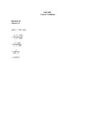
Item Number: 1<br />
Key: D<br />
Solution<br />
Because the autocorrelation function is zero starting with lag 2, this must be an MA(1) model.<br />
Then,<br />
−θ<br />
− .4 = ρ = , −.4 − .4 θ =−θ ,.4 θ − θ + .4 = 0.<br />
1<br />
2 2<br />
1 2<br />
1 1 1 1<br />
1+<br />
θ1<br />
This quadratic equation has two roots, 0.5 and 2. Because the coefficient’s absolute value must<br />
be less than 1, only 0.5 is acceptable.<br />
C4<strong>2001</strong>A
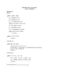
Item Number: 2<br />
Key: B<br />
Solution<br />
e λ 1<br />
The posterior distribution is π( λ|2)<br />
2! 3<br />
with parameters 3 and 3/4. The variance is 3(3/4) 2 = 27/16.<br />
−λ<br />
2<br />
−λ/3 2 −4 λ/3<br />
∝ e ∝ λ e which is a gamma distribution<br />
C4<strong>2001</strong>A
Item Number: 3<br />
Key: C<br />
Solution<br />
( 1− 3) + ( 2− 3) + ( 3− 3) + ( 4− 3) + ( 5−3)<br />
2 2 2 2 2<br />
2<br />
2<br />
= = =<br />
µ σ<br />
( 1− 3) + ( 2− 3) + ( 3− 3) + ( 4− 3) + ( 5−3)<br />
4 4 4 4 4<br />
µ<br />
4<br />
= = 6.8<br />
5<br />
µ<br />
4<br />
6.8<br />
γ<br />
2<br />
= = =<br />
4 1.7<br />
σ 4<br />
5<br />
2<br />
C4<strong>2001</strong>A
Item Number: 4<br />
Key: E<br />
Solution<br />
The calculations for each possibility are:<br />
Censored at 1 Censored at 2 Censored at 3 Censored at 4 Censored at 5<br />
Time d Y S $ d Y S $ d Y S $ d Y S $ d Y S $<br />
1 0 5 1 1 5 .80 1 5 .80 1 5 .80 1 5 .80<br />
2 1 4 .75 0 4 .80 1 4 .60 1 4 .60 1 4 .60<br />
3 1 3 .50 1 3 .53 0 3 .60 1 3 .40 1 3 .40<br />
4 1 2 .25 1 2 .27 1 2 .30 0 2 .40 1 2 .20<br />
5 1 1 0 1 1 0 1 1 0 1 1 0 0 1 .20<br />
This result may also be obtained by general reasoning. If the lapse occurs late, then the “death”<br />
times come earlier, leading to lower survival probabilities. If the lapse occurs early, then the<br />
“death” times come later, leading to higher survival probabilities.<br />
C4<strong>2001</strong>A
Item Number: 5<br />
Key: C<br />
Solution<br />
This is testing H0: β4 = β5<br />
= 0, which is a joint test on several regression coefficients.<br />
The key formula is 5.21 (p.130 of Pindyck and Rubinfeld).<br />
2<br />
We are given: R UR = 094 .<br />
Also, we know: N = 42, k = 5 (total number of coefficients to be estimated) and q = 2<br />
Using 5.21, we obtain F =<br />
b094 . − 0915 . g / 2<br />
b1 − 094 . g / b42 −5g<br />
= 77 . .<br />
C4<strong>2001</strong>A
Item Number: 6<br />
Key: C<br />
Solution<br />
The number of expected claims (e) is proportional to the number of exposure units (n). Let e =<br />
cn. Using Bühlmann credibility and partial credibility gives:<br />
25 1 25/ 25<br />
= = c =<br />
100 2 25/ c+ k 25+<br />
ck<br />
Therefore ck = 25.<br />
When we have 100 expected claims,<br />
100/ c 100 100<br />
Z = = = = 0.80.<br />
100/ c+ k 100+ ck 100+<br />
25<br />
C4<strong>2001</strong>A
Item Number: 7<br />
Key: D<br />
Solution<br />
Following Example 2.71 in Loss Models (with no denominator because this problem has no<br />
deductible), the contribution to the likelihood function for a loss (x) below 1000 is<br />
1 x / θ<br />
f ( x)<br />
= θ − e<br />
−<br />
−1000/<br />
θ<br />
while for observations censored at 1000 it is 1 − F(1000)<br />
= e . The<br />
likelihood function is:<br />
⎛ ⎞⎛ ⎞<br />
j<br />
L( θ) = ⎜ θ e ⎟⎜ e ⎟=<br />
θ e<br />
62 100<br />
−1 − x / θ −1000/ θ −62 − (28,140+<br />
38,000)/ θ<br />
∏<br />
The logarithm and its derivative are:<br />
∏<br />
⎝ j= 1 ⎠⎝ j=<br />
63 ⎠<br />
l( θ) =−62ln( θ ) −66,140θ<br />
l′ ( θ) =− 62θ + 66,140θ<br />
−1 −2<br />
−1<br />
Setting the derivative equal to zero yields θ ˆ = 66,140/62= 1067 .<br />
C4<strong>2001</strong>A
Item Number: 8<br />
Key: E<br />
Solution<br />
ˆ d<br />
1 1 1<br />
( 14<br />
i<br />
B ) = ∑ = + + = 4.65<br />
Qt ( ) 0.25+ 0.15+ 0.5 0.15+<br />
0.5 0.5<br />
ti≤14<br />
i<br />
C4<strong>2001</strong>A
Item Number: 9<br />
Key: D<br />
Solution<br />
ESSR<br />
− ESSUR<br />
F statistic = bN − kg b g<br />
q ESS<br />
N = 100<br />
k = 3<br />
q = 2<br />
Series I: F = 97<br />
Series II: F = 97<br />
Series III: F = 97<br />
b<br />
b<br />
UR<br />
g<br />
3552. 2−<br />
32338 .<br />
2 32338 .<br />
b<br />
b<br />
g<br />
13005 . − 11318 .<br />
2 11318 .<br />
b<br />
b<br />
g<br />
g<br />
g<br />
237. 0−<br />
2111 .<br />
2 2111 .<br />
b<br />
g<br />
g<br />
= 4. 78,<br />
Fail to reject<br />
= 7. 23,<br />
Reject<br />
= 595 . , Reject<br />
C4<strong>2001</strong>A
Item Number: 10<br />
Key: A<br />
Solution<br />
= E N A E X A = b2 / 3gb990g<br />
= 660<br />
= E N B E X B = b4 /<br />
276g<br />
= 368<br />
c = h = c = h c = h = b gb g = =<br />
c h c h c 1 2 h b gb gb g<br />
PcA500h 12/ 28 3/ 7 and Pc B500h<br />
4 / 7<br />
E L A<br />
E L B<br />
P L 500 A P N 1A P X 500 A 4 / 9 1/ 3 4 / 27 12/<br />
81<br />
P L = 500 B = P N = 2 B P X = X = 250 B = 4 / 9 2 / 3 2 / 3 = 16 / 81<br />
⇒ = = =<br />
( ) ( )<br />
E⎡⎣L2 L1 = 500⎤⎦<br />
= 3/7660+ 4/7368=<br />
493<br />
C4<strong>2001</strong>A
Item Number: 11<br />
Key: D<br />
Solution<br />
2 2<br />
( ) ( ) [ ] 2<br />
VHM = ⎡<br />
⎣<br />
1/2660 + 1/2368 ⎤<br />
⎦<br />
− 514 = 285,512− 264,196=<br />
21,316<br />
Total variance = 296,962<br />
EPV = Total variance – VHM = 275,646<br />
EPV<br />
1<br />
k = = 12.9314⇒ Z = = 0.07178<br />
VHM<br />
1+<br />
k<br />
Bühlmann credibility premium Z ( Z)<br />
= 500 + 514 1− = 513<br />
C4<strong>2001</strong>A
Item Number: 12<br />
Key: E<br />
Solution<br />
The distribution function is ( )<br />
yields the K-S statistic:<br />
F<br />
1<br />
x<br />
−3<br />
∫ 2(1 ) 1 . From it, the following table<br />
0<br />
2<br />
F x = + t dt = −<br />
( 1+<br />
x)<br />
x .1 .2 .5 1.0 1.3<br />
F x<br />
b g .174 .306 .556 .75 .811<br />
x −<br />
0 .2 .4 .6 .8<br />
bx<br />
g .2 .4 .6 .8 1.0<br />
n<br />
n +<br />
The K-S statistic is 0.189.<br />
F<br />
Max diff. .174 .106 .156 .15 .189<br />
C4<strong>2001</strong>A
Item Number: 13<br />
Key: B<br />
Solution<br />
2<br />
2<br />
∑c i h ∑c 2i<br />
2h<br />
Divide the first equation by Y − Y X − X<br />
2<br />
2<br />
∑cYi<br />
− Yh ∑cX3i<br />
− X3h<br />
to get the equations:<br />
and the second equation by<br />
r<br />
YX<br />
2<br />
sX<br />
s<br />
2 X3<br />
= $ 2 + $ 3 rX X = $ *<br />
2 + $ *<br />
β β β β 3r<br />
s s<br />
Y<br />
Y<br />
X X<br />
2 3 2 3<br />
r<br />
YX<br />
3<br />
sX<br />
s<br />
2<br />
X3<br />
= β $ rX X + β $ = β $ r<br />
2 3<br />
X2X<br />
+ β $<br />
3<br />
s<br />
s<br />
* *<br />
2 3 2 3<br />
Y<br />
Y<br />
Solve these equations for $ *<br />
rYX − r . . .<br />
2 YX r<br />
3 X 04 09 06<br />
2X<br />
−<br />
3<br />
β 2 =<br />
=<br />
2 2<br />
1−<br />
r 1−<br />
0.<br />
6<br />
X X<br />
2 3<br />
b gb g<br />
b g<br />
= −0.<br />
22.<br />
C4<strong>2001</strong>A
Item Number: 14<br />
Key: C<br />
Solution<br />
σ<br />
2<br />
H<br />
di<br />
15 20 13<br />
20 = ∑ = + + = 0.0144<br />
2 2 2<br />
Y 100 65 40<br />
( )<br />
ti<br />
≤20<br />
σ H b20g = 0. 0144 = 012 .<br />
i<br />
C4<strong>2001</strong>A
Item Number: 15<br />
Key: A<br />
Solution<br />
=zτ<br />
µ $ S $ btgdt<br />
τ<br />
0<br />
b g b g b g b g<br />
= 10 . × 1 + 085 . × 7 + 05885 . × 9 + 03972 . × 8 = 1542 .<br />
z<br />
D<br />
L V$ $ S$<br />
di<br />
µ = τ N M<br />
2<br />
τ<br />
∑ btgdt<br />
ti<br />
i=<br />
1<br />
QP Yib Yi − dig<br />
O<br />
2 2 2<br />
= 14424 . × 00018 . + 8474 . × 00068 . + 3178 . × 00120 .<br />
= 0.9840<br />
The 95% confidence interval is:<br />
15.42± 1.96×<br />
0.9840<br />
b<br />
135 . , 17.<br />
4<br />
g<br />
C4<strong>2001</strong>A
Item Number: 16<br />
Key: C<br />
Solution<br />
The Weibull density function is<br />
.5<br />
.5 ( x / θ )<br />
θ − −<br />
f ( x) = .5( x ) e . Therefore the likelihood function is<br />
The logarithm and its derivative are:<br />
10<br />
.5<br />
−.5<br />
−( x j/ θ)<br />
L( θ) = ∏.5( xjθ)<br />
e<br />
j=<br />
1<br />
−.5<br />
10<br />
10 −5<br />
∏ xj<br />
θ<br />
j=<br />
1<br />
⎛ ⎞<br />
= (.5)<br />
e<br />
∑<br />
⎜ ⎟<br />
⎝ ⎠<br />
∝ θ<br />
−.5<br />
−5 −488.97θ<br />
e<br />
.<br />
−.5 10 .5<br />
−θ<br />
x<br />
j = 1<br />
j<br />
l( θ) =−5lnθ−488.97θ<br />
l′ =− +<br />
−.5<br />
−1 −1.5<br />
( θ) 5θ 244.485 θ .<br />
Setting the derivative equal to zero yields<br />
2<br />
ˆ (244.485/5) 2391.<br />
θ = =<br />
C4<strong>2001</strong>A
Item Number: 17<br />
Key: E<br />
Solution<br />
The estimated variance of the forecast errors is the sum of the squares of the error terms divided<br />
by T − p − q. In this case, after 100 observations, the sum of the squares of the error terms must<br />
equal 98, because the sum divided by b100 −1−1g, or 98, is 1.0.<br />
The 101 st observation introduces a new error term equal to 188−197, or − 9. The square of that<br />
term is 81. Adding 81 to the previous sum of 98 gives a new total of 179. Dividing 179 by<br />
b101−1−1g, or 99, gives a new estimated variance of 1.8.<br />
C4<strong>2001</strong>A
Item Number: 18<br />
Key: A<br />
Solution<br />
− 5 .2 6 1.2<br />
The posterior distribution is ( |0) e λ −<br />
(.5)5 e λ −<br />
(.5).2e λ −<br />
π λ<br />
2.5 e λ −<br />
∝ ⎡<br />
⎣<br />
+ ⎤<br />
⎦<br />
= + .1 e<br />
λ . The<br />
∞<br />
−6 1.2<br />
normalizing constant can be obtained from 2.5 e λ − λ<br />
∫<br />
⎡ + .1 e ⎤dλ<br />
= .5<br />
0 ⎣<br />
⎦ and therefore the exact<br />
−6λ<br />
−1.2λ<br />
posterior density is π( λ|0) = 5 e + .2e<br />
. The expected number of claims in the next year is<br />
∞<br />
−6λ<br />
−1.2λ<br />
5 5 5<br />
the posterior mean, E( Λ |0) = ∫ λ[5 e + .2 e ] dλ<br />
= + = = .278.<br />
0<br />
36 36 18<br />
C4<strong>2001</strong>A
Item Number: 19<br />
Key: B<br />
Solution<br />
There are 365 observations, so the expected count for k accidents is<br />
produces the following table:<br />
− .6 k<br />
e (.6)<br />
365pk<br />
= 365 which<br />
k!<br />
No. of accidents Observed Expected Chi-square<br />
0 209 200.32 0.38<br />
1 111 120.19 0.70<br />
2 33 36.06 0.26<br />
3 7 7.21 1.51**<br />
4 3 1.08<br />
5 2 0.14*<br />
*This number is 365 minus the sum of the other expected counts.<br />
**The last three cells must be grouped to get the expected count above 5. The calculation for the<br />
test statistic is (12 – 8.43) 2 /8.43 = 1.51. The total of the chi-square numbers is the test statistic of<br />
2.85.<br />
C4<strong>2001</strong>A
Item Number: 20<br />
Key: E<br />
Solution<br />
The likelihood ratio test statistic is ( − 382.4+ 385.9)<br />
⋅ 2= 7.<br />
C4<strong>2001</strong>A
Item Number: 21<br />
Key: C<br />
Solution<br />
8<br />
2<br />
20<br />
2<br />
⎛Yt<br />
−α⎞ ⎛Yt<br />
−α<br />
⎞<br />
∑ ∑ to be a minimum. Setting the derivative equal to<br />
We need for S( α)<br />
= ⎜ ⎟ + ⎜ ⎟<br />
t= 1⎝ 0.4 ⎠ t=<br />
9 ⎝ 0.6 ⎠<br />
8 20<br />
1 1<br />
zero produces the equation S′ ( α) = 2( Yt<br />
− α) + 2( Yt<br />
− α) = 0.<br />
.4 t= 1 .6 t=<br />
9<br />
produces the equation:<br />
∑ ∑ Multiplying by 0.6<br />
0 = 3(8Y<br />
− 8 α) + 2(12Y<br />
−12 α)<br />
1 2<br />
0 = 24Y<br />
+ 24Y<br />
−48α<br />
1 2<br />
αˆ = .5 Y + .5Y<br />
1 2<br />
C4<strong>2001</strong>A
Item Number: 22<br />
Key: E<br />
Solution<br />
Ο=4<br />
E = (.29 − .27) + (.35 − .27) + (.41 − .27) + 7.465 ( − .27)<br />
= 1.605<br />
b<br />
Chi-square statistic = 4 − 1605 . / 1605 . = 357 .<br />
The 0.05 level of significance is 3.84, so the answer is (E).<br />
g<br />
2<br />
C4<strong>2001</strong>A
Item Number: 23<br />
Key: B<br />
Solution<br />
The Bühlmann-Straub credibility factor is<br />
n<br />
w +<br />
n +<br />
a<br />
v<br />
m<br />
which goes to<br />
n<br />
n +<br />
w<br />
a<br />
as m goes to infinity.<br />
C4<strong>2001</strong>A
Item Number: 24<br />
Key: B<br />
Solution<br />
With a lognormal error component, the linear model should be for the logarithm of the<br />
observation. A model that conforms to the description is<br />
lnY = α + α D + β X + ε .<br />
* * * *<br />
1 2 1<br />
Exponentiating both sides yields<br />
* * * *<br />
α1 α2 D β1<br />
X ε<br />
Y = e e e e<br />
and then defining an unstarred quantity as its starred version exponentiated, we have<br />
Y<br />
= αα β ε<br />
D X<br />
1 2 1<br />
.<br />
Note that when D is 1, the value of Y is multiplied by<br />
2<br />
α and so the hypothesis to test is if this<br />
value is equal to 0.8.<br />
C4<strong>2001</strong>A
Item Number: 25<br />
Key: C<br />
Solution<br />
The function of interest is f ( αβ , ) = α+ 10 β.<br />
The partial derivatives are 1 and 10 and so the<br />
variance can be estimated as<br />
⎡αˆ 2<br />
⎤⎡1<br />
⎤<br />
σˆ<br />
[ 110]<br />
Var ˆ<br />
f<br />
= ⎢ ˆ⎥⎢ 10<br />
⎥<br />
⎣β<br />
⎦⎣ ⎦<br />
⎡ 0.00055 −0.00010⎤⎡ 1⎤<br />
= [ 110]<br />
⎢<br />
0.00010 0.00002<br />
⎥⎢<br />
10<br />
⎥<br />
⎣−<br />
⎦⎣ ⎦<br />
= 0.00055− 2× 0.00010× 10+ 0.00002×<br />
100<br />
= 0.00055<br />
and so the standard deviation is the square root, or 0.02345.<br />
C4<strong>2001</strong>A
Item Number: 26<br />
Key: A<br />
Solution<br />
Following Klein and Moeschberger with the time scale shifted by 1997:<br />
T i L i R i d i Y i P[ L< l | L<<br />
3]<br />
i<br />
0 0 2 6<br />
1 0 2 5<br />
2 0 2 4 15 (99/160) ⋅ 0 = 0<br />
0 1 1 3<br />
1 1 1 2 16 (9/10) ⋅ (11/16) = 99/160<br />
0 2 0 1 10 9/10<br />
9 99<br />
P[ L= 1| L< 3] = P[ L< 2| L< 3] − P[ L< 1| L< 3]<br />
= − = 0.28125<br />
10 160<br />
C4<strong>2001</strong>A
Item Number: 27<br />
Key: E<br />
Solution<br />
From formula 15.41:<br />
yt<br />
825 784 710 918<br />
zt<br />
= , z6 = , z18 = , z30 = , z42<br />
=<br />
y%<br />
843 804 740 905<br />
t<br />
From formula 15.42:<br />
~z 6 =<br />
1<br />
4bz6 + z18 + z30 + z42g<br />
~ z<br />
1 . . . . .<br />
6 = 4<br />
09786 + 09751+ 09595+ 10144 = 09819<br />
b<br />
Adjustment factor = 12/11.9607 =1.0033<br />
g<br />
z<br />
y<br />
6<br />
a<br />
42<br />
= .9819*1.0033=<br />
0.9851<br />
918<br />
= = 932<br />
0.9851<br />
C4<strong>2001</strong>A
Item Number: 28<br />
Key: E<br />
Solution<br />
Die/Spinner Prior probability Probability of<br />
getting a 12<br />
Posterior<br />
Probability<br />
AX 1/4 3/4× 1/2= 3/8 1/4<br />
AY 1/4 3/4× 1= 3/4 1/2<br />
BX 1/4 1/4× 1/2= 1/8 1/12<br />
BY 1/4 1/4× 1= 1/4 1/6<br />
Total 1 3/2 1<br />
Die/Spinner Expected Value Posterior Probability Expected Value ×<br />
posterior probability<br />
AX (3/4)(1/2)(12+c) 1/4 1.125+3/32c<br />
AY (3/4)(12) 1/2 4.5<br />
BX (1/4)(1/2)(12+c) 1/12 0.125+1/96c<br />
BY (1/4)(12) 1/6 0.5<br />
Total 1 6.25+10/96c<br />
Because the expected value is 10, 6.25+10/96c = 10, so c = 36.<br />
C4<strong>2001</strong>A
Item Number: 29<br />
Key: D<br />
Solution<br />
Summing the ranks of the A’s (being careful to average for ties) gives<br />
(1+2+6+6+8.5+8.5+10+11+13.5+20) = 86.5 (or 123.5 working with B’s).<br />
*<br />
E R = 105, Var R = 175,so r =± 1.398giving p=<br />
0.162.<br />
( ) ( )<br />
H0 H0<br />
C4<strong>2001</strong>A
Item Number: 30<br />
Key: C<br />
Solution<br />
The maximum likelihood estimate of the mean, θ, is the sample mean, 367.9.<br />
2<br />
Two years of inflation at 5% inflates this scale parameter toθ = 1.05 (367.9) = 405.6.<br />
The expected amount paid per loss is<br />
E( X ∧1000) −EX<br />
( ∧100)<br />
= − − +<br />
−1000/405.6 −100/405.6<br />
405.6(1 e 1 e )<br />
= 283.<br />
C4<strong>2001</strong>A
Item Number: 31<br />
Key: A<br />
Solution<br />
L<br />
( â)<br />
β1 β 2<br />
β<br />
⎛<br />
3<br />
⎛ e ⎞⎛ e ⎞⎛e<br />
⎞⎞<br />
= ⎜⎜ β1 β2 β ⎟⎜<br />
3 β2<br />
β ⎟⎜<br />
3 β ⎟<br />
3<br />
e + e + e e + e e ⎟<br />
⎝⎝ ⎠⎝ ⎠⎝ ⎠⎠<br />
C4<strong>2001</strong>A
Item Number: 32<br />
Key: A<br />
Solution<br />
2 3<br />
∑∑<br />
i=<br />
1<br />
( − )<br />
mij xij xi<br />
i= 1 j=<br />
1<br />
2020<br />
vˆ = = = 505<br />
2<br />
2+<br />
2<br />
2<br />
∑<br />
( 3−1)<br />
2<br />
( − ) −ˆ ( 2−1)<br />
m x x v<br />
2<br />
4800−<br />
505 4295<br />
i i<br />
i=<br />
1<br />
ˆ = = = = 114.5333<br />
2 2 2<br />
1 2<br />
m−<br />
m<br />
100− ( 1/100) ( 25 + 75 ) 37.5<br />
∑ i<br />
m i=<br />
1<br />
a<br />
∑<br />
ˆ vˆ<br />
k = = 4.4092<br />
aˆ<br />
25<br />
Zˆ 1<br />
= = 0.850074<br />
25 + kˆ<br />
75<br />
and Zˆ 2<br />
= = 0.944475<br />
75+<br />
kˆ<br />
ZX ˆ<br />
Zˆ<br />
+ Zˆ<br />
X<br />
+ Zˆ<br />
1 1 2 2<br />
ˆ = = 105.4208<br />
µ<br />
1 2<br />
Bühlmann credibility premium Zˆ ( ) ( Z ˆ<br />
)( µ ˆ )<br />
= 97 + 1− = 98.26<br />
1 1<br />
C4<strong>2001</strong>A
Item Number: 33<br />
Key: A<br />
Solution<br />
According to a statement on page 159 of Pindyck and Rubinfeld, the estimator is unbiased.<br />
C4<strong>2001</strong>A
Item Number: 34<br />
Key: D<br />
Solution<br />
The observations are right and left truncated and the truncation depends upon the report year.<br />
For report year 1997 only claims settled at durations 1 and 2 can be observed, so the denominator<br />
must be the sum of those two probabilities. For 1998, only durations 0 and 1 can be observed<br />
and for 1999 only duration 0 can be observed. Calculation of the denominator probabilities is<br />
summarized below.<br />
Probabilities<br />
Year<br />
Year Settled<br />
Reported 1998 1999<br />
1997 b1− pgp<br />
1− p p<br />
1998 1− p<br />
Sum<br />
(Denominator)<br />
− p p + p<br />
2<br />
b g b1 g b1<br />
g<br />
b g b1− pgp<br />
b1 − p gb1+<br />
pg<br />
b g b1− pg<br />
1999 1− p<br />
The likelihood function is:<br />
( )<br />
( ) ( )<br />
( 1+<br />
p)<br />
11<br />
2<br />
( )<br />
( ) ( )<br />
( )<br />
( ) ( )<br />
( )<br />
( ) ( )<br />
( )<br />
( )<br />
3 1 5 2 4<br />
⎛ 1− p p ⎞⎛ 1− p p ⎞⎛ 1−p ⎞⎛ 1− p p ⎞ ⎛ 1−<br />
p ⎞<br />
L( p)<br />
= ⎜ 1− p p 1+ p ⎟⎜ 1− p p 1+ p ⎟⎜ 1− p 1+ p ⎟⎜ 1− p 1+ p ⎟ ⎜ 1−<br />
p ⎟<br />
⎝ ⎠⎝ ⎠⎝ ⎠⎝ ⎠ ⎝ ⎠<br />
3 1 5 2<br />
⎛ 1 ⎞⎛ p ⎞⎛ 1 ⎞⎛ p ⎞<br />
= ⎜<br />
1 p ⎟⎜<br />
1 p ⎟⎜<br />
1 p ⎟⎜<br />
1 p ⎟<br />
⎝ + ⎠⎝ + ⎠⎝ + ⎠⎝ + ⎠<br />
3<br />
p<br />
=<br />
The loglikelihood is l( p) = 3ln( p) − 11ln( 1+<br />
p)<br />
Take the derivative with respect to p to obtain the equation to solve:<br />
3 11<br />
− = 0<br />
p 1 + p<br />
b<br />
g<br />
The solution is p $ = 3 .<br />
8<br />
C4<strong>2001</strong>A
Item Number: 35<br />
Key: E<br />
Solution<br />
( ) ( )<br />
t d Y ∆ H % 4 −t<br />
H t K t*<br />
i<br />
( t)<br />
∆Vˆ<br />
⎡ ⎣<br />
H%<br />
( t)<br />
⎤ t* = ⎦ b Kbt * g<br />
∆ % ˆ ( ) Kt (*)<br />
∆V ⎡H%<br />
t ⎤<br />
⎛ ⎞<br />
⎜<br />
b<br />
⎣ ⎦ b<br />
⎟ ⎝ ⎠<br />
1 1 9 0.1111 0.01235 1.0000 0.000 0.0000 0.000000<br />
3 2 8 0.2500 0.03125 0.3333 0.741 0.0617 0.001905<br />
5 1 5 0.2000 0.04000 −0.3333 0.741 0.0494 0.002439<br />
8 2 3 0.6667 0.22222 −1.3333 0.000 0.0000 0.000000<br />
10 1 1 1.0000 1.00000 −2.0000 0.000 0.0000 0.000000<br />
h ˆ(4) = 0.1111<br />
2<br />
σ [ hˆ<br />
(4)] = 0.00434<br />
2<br />
Lower confidence limit:<br />
1.96 0.00434/0.1111<br />
0.1111e − = 0.035<br />
Upper confidence limit:<br />
1.96 0.00434/0.1111<br />
0.1111e = 0.355<br />
C4<strong>2001</strong>A
Item Number: 36<br />
Key: D<br />
Solution<br />
See page 555 of Pindyck and Rubinfeld. The variance is 1/T, not T, and the statement is then<br />
only true for large displacements.<br />
C4<strong>2001</strong>A
Item Number: 37<br />
Key: B<br />
Solution<br />
The first step is to get the posterior distribution of P given no claims:<br />
π( p|0) ∝ f(0| p) π( p)<br />
= e<br />
−+ 1 0.01p<br />
(0.01)<br />
0.01p<br />
∝ e < p <<br />
,0 100<br />
The normalizing constant can be found from<br />
∫<br />
100 100<br />
0.01p<br />
0.01p<br />
0<br />
e dp = 100e = 100( e− 1) = 171.83.<br />
0<br />
The posterior density is<br />
Then,<br />
1<br />
π = < <<br />
171.83<br />
0.01p<br />
( p|0) e ,0 p 100.<br />
1 100<br />
171.83 171.83<br />
100<br />
0.01 p<br />
.5<br />
Pr( P > 50|0) = ∫ e dp = ( e− e ) = 0.622.<br />
50<br />
C4<strong>2001</strong>A
Item Number: 38<br />
Key: B<br />
Solution<br />
µ ( p) = 1−0.01p<br />
µ = E[ µ ( p)] = E(1− 0.01 p) = 1− 0.01(50) = 0.5<br />
2<br />
100<br />
a = Var[ µ ( p)] = Var(1− 0.01 p) = 0.0001 Var( p) = 0.0001 = 1/12<br />
12<br />
vp ( ) = 1−0.01p<br />
v= Evp [ ( )] = 0.5<br />
k = v/ a= (1/2)/(1/12) = 6<br />
Z = 4/(4+ 6) = 0.4<br />
P = 0.4(5/4) + 0.6(0.5) = 0.8<br />
c<br />
The number of claims is Poisson, so the mean and variance are the Poisson parameter, 1 – 0.01p.<br />
The mean and variance of p come from the uniform distribution.<br />
C4<strong>2001</strong>A
Item Number: 39<br />
Key: E<br />
Solution<br />
For a mixture, the mean and second raw moments are a mixture of the component means and<br />
second raw moments. Therefore,<br />
E( X) = p(1) + (1 − p)(10) = 10−9p<br />
2<br />
E( X ) = p(2) + (1 − p)(200) = 200−198p<br />
Var X p p p p<br />
2 2<br />
( ) = 200−198 −(10− 9 ) = 100−18 − 81 = 4.<br />
The only positive root of the quadratic equation is p = 0.983.<br />
C4<strong>2001</strong>A
Item Number: 40<br />
Key: C<br />
Solution<br />
s<br />
2<br />
=<br />
∑<br />
2<br />
ε$<br />
i 967<br />
1934<br />
N − 2<br />
= 5<br />
= .<br />
2<br />
β$<br />
s<br />
2<br />
s 1934 .<br />
= = = 0.<br />
0967<br />
2<br />
x 2000<br />
∑<br />
i<br />
s<br />
β$<br />
= 031 .<br />
C4<strong>2001</strong>A