Download
1 / 44
440 likes | 461 Views
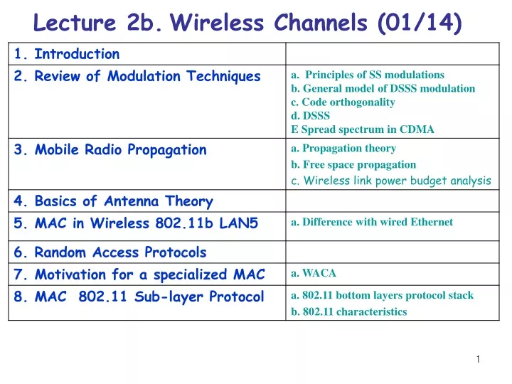
Lecture 2b. Wireless Channels (01/14). 1.Introduction. The Electromagnetic Spectrum Radio Transmission Microwave Transmission Infrared and Millimeter Waves Lightwave Transmission

E N D
1.Introduction • The Electromagnetic Spectrum • Radio Transmission • Microwave Transmission • Infrared and Millimeter Waves • Lightwave Transmission • In vacuum, all electromagnetic waves travel at the same speed, no matter what their frequency. This speed is the speed of light-c, is about 1 foot (30cm)/ns. In copper or fiber the speed slows to about 2/3 of this value and is slightly frequency dependent. • The relation between frequency , wavelength , and speed –c is . • As a rule of thumb, when is in meters and is in MHz- .
2. Review of Modulation Techniques • 1. Microwave voice/data transmissions:No AM. • Data-modulate the carrier wave using: • PM, FM, and SS modulation techniques. • 2a. Links (channels) are separated with: FDMA. • Voice data-to encode signal digitally use:PCM • 3a. Several voice signals in one channel • are separated by: TDMA
A, , and f BPSK: 0° or 180°, QPSK 0°, 90°, 180°, 270° A higher Kf value can be used in modulating the audio signal, Higher Kf value decreases the signal error rate. However, decoding an FM signal becomes very difficult at high Kf, So we cannot increase Kf to use FM transmission in a wide frequency band. In the radio spectrum, the available bandwidth exceeds the necessary data rate. For instance, FM radio stations have about 100 kHz, bandwidth of an audio signal 20 kHz. Spread spectrum techniques are necessary to for efficient use of a wide frequency band at low error rates. Modulation Techniques (cont)
Shannon’s law shows the relationship between analog Channel bandwidth and digital channel capacity: When the SNR<below 1(wireless channel is noisy channel), less than 1 bit can be transferred by each sample. If the SNR ratio = 3, and the C=<2B. Transmission Rate R is provided Equality is achieved only when SNR is infinity In practice: impossible to create an encoding scheme that allows accurate transmissions near to the Shannon limit. SS modulation allows to more closely approach the Shannon's limit, by transmitting at a low SNR.
a. Principles of SS modulation • The most important parameter in any SS system is • the processing gainGp: This value measures the ratio of Transmitted RF bandwidth W to the narrowband information rate C. A system with a low signal-to-noise ratio must have a high processing gain Gp in order to recover the originalsignal. • Types of Spread Spectrum Modulation: • Direct Sequence Spread Spectrum (DSSS) • Frequency Hopping Spread Spectrum (FHSS)
b. General model of DSSS modulations BPSK or QPSK “chipping”.
c. Code orthogonality Two vectors called orthogonal if their inner product is 0(Orthogonal in code space has the same meaning as in standard space).Code for a certain user should be orthogonal to other codes, and should have a good autocorrelation. Two vectors (2,5,0) and (0,0,17); (2,5,0)*(0,0,17)=0+0+0=0;The vectors (1,2,3) and (4,2,-6) are not (inner product -10);(1,2,3) and (4,2,-3 are “almost” orthogonal (-1which is close to zero). Barker code (+1,-1,+1,+1,-1,+1,+1+1,-1,-1,-1),has good autocorrelation, (inner product with itself is large 11). But if this Barker code is shifted1 chip, the correlation drops to a value of 1. It stays at this low until the code matches itself again perfectly. This helps to synchronize a receiver with the data stream. The matching process helps the receiver, to reconstruct the original data. DSSS
A and B, want to send data, CDMA assigns the following unique and orthogonal key sequences: key for senderA, Key for sender B. ; A wants to send the bit , sender B sends . To illustrate this example, let us assume that we code a binary 0 as -1, and binary 1 as +1. We can then apply the standard addition and multiplication rules. Both senders spread their signal using their key as chipping sequence (the term “spreading” here refers to the multiplication on the data bit with the whole chipping sequence). Both signals are then transmitted at the same time using the same frequency, the signals superimpose in space. (No interference, no noise from this simple example), If the signals have the same strength at the receiver, the following signal C is received at a receiver DSSS
Receiver now wants to receive data from sender A and, therefore, tunes in to the code of A, i.e., applies A’s code for dispreading: DSSS It is much larger than 0, the receiver detects a binary 1 (A has sent 1). Tuning in to sender B, i.e., applying B’s code gives The result is negative, so a 0 has been detected (B has sent bit 0).
d. DSSS (Cont) DSSS
DSSS (Cont) Gp is determined from:PN sequence bit rate/the data signal information rate. For example: If the information signal is transmitted at 9600 bps. The PN sequence has a bit rate of 38,400 bps. The resulting, transmitted bit rate is 38,400 bps, so In systems, where noise is small relative to the transmission signal power of each user, DSSS can be effective for reliable transmission of several simultaneous signals. DSSS
CELLULAR e. Spread Spectrum in CDMA • CDMA: uses SS (DSSS or FHSS) encoding scheme • Unique code assigned to each user; (code set partitioning) Used mostly in wireless broadcast channels (cell., satellite) • All users in the same channel share the same frequency, but each user has own “chipping” sequence (i.e., code) • Chipping sequence like a mask: used to encode the signal • Encoded signal =(original signal) X (chipping sequence) • To make CDMA work, chipping sequences must be chosen orthogonal to each other. Global System Mobile uses FM and TDMA
CDMA: two-sender interference CELLULAR 1 2
3. General model of FHSS modulation “chipping”.
FHSS 1 2 3 4 4 FHSS is an ideal for a WLAN in a noisy frequency band ! During any one hop, the signal is vulnerable to noise in that frequency band, but it will soon move to another frequency with less noise. This new band will be sufficiently removed from the previous noisy band
FHSS hops If stations use the same seed of the PN number, they stay synchronized in time. Dwell time, is an adjustable parameter, but must less than 400 msec. They will hop to the same frequencies simultaneously • FHSS advantages for WLAN • WLAN systems can overlap without • interference • • Immunity from noise and • interference • • Resistance to radio reflections • (multipath transmission) • • High data transfer capacity • • Low price for TR and R FHSS provides a security since an intruder, who does not know the hopping sequence or dwell time cannot overhear on transmissions. P 23 for Japan 79hops, each1-MHz wide FHSS offers good resistance to multipath fading GHz 2.4 2.483
Example: Bluetooth Frequency Hopping 1Mhz • frequency hopping spread spectrum • 2.402 GHz + k MHz, k=0, …, 78 • 1,600 hops per second • GFSK modulation • 1 Mb/s symbol rate • transmit power • 0 dBm (up to 20 dBm with power control) . . . 79 1 2 3 83.5 Mhz
4. TDMA • Compared to FDMA, TDMA offers a much more flexible scheme, • No certain frequency is necessary, i.e., the receiver can stay at the same frequency the whole time. • Uses one frequency. • Simple receivers and transmitters. • Many different MAC algorithms exist. • Listening to different frequency channels at the same time is quite difficult, listening to many channels separated in time means TDMA+FDMA. • Almost all MAC schemes for wired networks work according to this principle (Ethernet, Token Ring). Classical Aloha; Slotted Aloha
5.Medium Access Protocol CSMA/CA When many users are located in the same area, and use the same wireless LAN at the same time, two different MAC methods are defined for signal multiplexing: 1.Distributed Coordination Function(DCF) (no control) 2. Point Coordination Function(PCF) (BS controls cell) The basic access mechanism, called the DCF, Each unit senses the medium before it starts to transmit. If the medium is free for several microseconds, the unit can transmit for a limited time. If the medium is busy, the unit will back-off for a random time before it senses again. It does not sense the channel while transmitting,
Medium Access with CSMA/CA (Cont) The basic access mechanism: • DCF = CSMA/CA algorithm: 2 methods. 1). Physical channel sensing. 2). Virtual channel sensing • Physical channel sensing (PCS):Like Ethernet • It does not sense the channel while transmitting, • CSMA/CD needs full-duplex channel • 802.11 all stations cannot hear each other 802.11 =802.3 + Positive Acknowledge Scheme 2. MACAW-Virtual Carrier Sense (VCS)
The 802.11 MAC Protocol (MACAW) 2. MACAW-Virtual Carrier Sense (VCS)using CSMA/CA. NAV-Network Allocation Vector -keeps other stations quiet
The 802.11 MAC Protocol: fragments (MACAW) 2. DCF-The use of virtual channel sensing using CSMA/CA. stop-and-wait protocol
802.11n 200 Mbps 802.11a,g point-to-point 802.11a,g 54 Mbps 802.11b W/MAX 5-11 Mbps UMTS/CDMA, CDMA2000 4 Mbps 3G 802.15.1 1 Mbps 3G 384 Kbps IS-95, CDMA, GSM 56 Kbps IS-95, CDMA, GSM 2G Indoor Outdoor Mid range outdoor Long range outdoor 10-30 m 50-200 m 200-4 Km 5 Km-20 Km a. Link characteristics of selected wireless network standards a
6. Mobile Radio Propagation • Free space loss • Two ray model • Slow fading • Fast fading • Delay spread Ground, Space, Sky, and Satellite waves
Radio Transmission (cont) troposphere (a) In the LF ( hertz), and MF ( hertz) bands, radio waves follow the curvature of the earth (ground). (b) In the HF ( hertz) band, they bounce off the ionosphere (space). Sky
What is the period of the moon according to Kepler’s law? Example 1 Solution The moon is located approximately 384,000 km above the earth. The radius of the earth is 6378 km. Applying the formula, we get Period = (1/100) (384,000 + 6378)1.5 = 2,439,090 s = 1 month According to Kepler’s law, what is the period of a satellite that is located at an orbit approximately 35,786 km above the earth? Example 2 Applying the formula, we get Period = (1/100) (35,786 + 6378)1.5 = 86,579 s = 24 h A satellite like this is said to be stationary to the earth. The orbit, as we will see, is called a geosynchronous orbit. Solution
a. Propagation mechanisms • Reflection:propagation wave reflected by object larger than wavelength results Large-scale fading. • Diffraction:wave obstructed by surface with sharp, irregular edges. • Scattering:wave hits loose objects smaller than wavelength; signal scattered in bunch of outgoing weaker signals are result Small-scale fading.
Reflection and diffraction of radio signals Scattering
multipath signals, Intersymbol interference In a time-dispersive medium the transmission rate R for a digital transmission is limited by the delay spread
b. Free space propagation • Consider an isotropic point source with power Pt. At distance d the radiated power is uniformly distributed over surface of a sphere. • Thus, received power Pr at distance d: • Ae = receiver antenna effective area • Gt= transmitter antenna antenna gain
Free Space Path lossLp Free space losses could be calculated by: Note: loss increases with carrier frequency. Lp = path loss (average propagation loss over wide area): Determined by distance, carrier frequency, land profile
Free-space path loss (Cont) 1500 MHz 150 MHz
c. Wireless Link Power Budget Analysis When operating at 3 Mbps, a WLAN system has transmission power of 15 dBm, and the receiver power must be at least –72 dBm. The communication power budget is therefore: To find how transmission distance and frequency affect the power budget, we can calculate the free space isotropic loss. This is the path loss incurred by an electromagnetic wave as it propagates in a straight line through a vacuum from one isotropic antenna to another. At any point around the antenna, the power density is:
Wireless Link Power Budget Analysis (cont) The power received is the product of the receiving antenna’s effective area and the power density: The free space isotropic loss is simply the inverse of the power, and is usually expressed in decibels: r: distance in meters : wavelength in meters f : frequency in Hertz m/second.
7. Basics of Antenna Theory • Antenna reciprocity -A transmitting antenna will transfer energy to the atmosphere with the same efficiency with which it transfers energy from the atmosphere to its terminals, Antenna reciprocity. • Isotropic -If an antenna is a point source that radiates power equally in all directions. • Power density at any point of sphere would be total radiated power, divided by the area of this sphere:
An isotropic antenna would radiate equally in all directions For transmission antenna, the directivity of the antenna is the ratio of max power density to isotropic power density. This ratio is usually expressed in decibels: The power density is always dependent on the orientation of the receiver, which is measured in polar coordinates. The direction of maximum power density is assigned to =0, =0.This point is also called theforesight of the antenna.
Transmission antenna (cont) A radiation diagramdescribes the ratio of the antenna’s power density at any orientation around the antenna to the isotropic power density: or gainof the antenna in this direction.
Receiving antenna (cont) • Effective areaof the antenna measures how well the antenna captures power, and is simply the ratio of the power received by the antennatothe power density at the point where the antenna is located. • The effective areaof the antenna can be much larger than the antenna geometric area. Because of the principle of reciprocity, the effective area of an antenna is related to the antenna gain by the following formula:
The polarization of the electromagnetic wave Polarization describes the direction of the electrical field of the electromagnetic wave There is also a perpendicular magnetic field, but we describe polarization in terms of the electric field. An antenna generally has a preferred polarization direction, and it is important that the polarization of the transmitting antenna matches the polarization of the receiving antenna.
Directional antenna radiation pattern. 3 dB beamwidth, the angle between points that are 3dB below the max power output. Omnidirectional antenna radiation pattern