

Analyzing County-Level COVID-19 Vaccination Rates in Texas: A New Lindley Regression Model

Departamento de Estatísca, Universidade Federal de Pernambuco, Cidade Universitária, Recife 52070-040, Brazil
*
Author to whom correspondence should be addressed.
COVID 2023, 3(12), 1761-1780; https://doi.org/10.3390/covid3120122
Submission received: 9 November 2023
/
Revised: 30 November 2023
/
Accepted: 2 December 2023
/
Published: 4 December 2023
(This article belongs to the Special Issue Analysis of Modeling and Statistics for COVID-19)
Abstract
:This work aims to study the factors that explain the COVID-19 vaccination rate through a generalized odd log-logistic Lindley regression model with a shape systematic component. To accomplish this, a dataset of the vaccination rate of 254 counties in the state of Texas, US, was used, and simulations were performed to investigate the accuracy of the maximum likelihood estimators in the proposed regression model. The mathematical properties investigated provide important information about the characteristics of the distribution. Diagnostic analysis and deviance residuals are addressed to examine the fit of the model. The proposed model shows effectiveness in identifying the key variables of COVID-19 vaccination rates at the county level, which can contribute to improving vaccination campaigns. Moreover, the findings corroborate with prior studies, and the new distribution is a suitable alternative model for future works on different datasets.
1. Introduction
The COVID-19 pandemic, caused by the novel coronavirus SARS-CoV-2, has had a profound impact on the world in the past few years. It has affected nearly every aspect of human life, causing significant disruptions to healthcare systems, economies, and social structures across the globe. The developments in the fight against the pandemic, mainly the vaccination, provided a crucial tool to protect individuals and communities against the virus and help to mitigate its spread.
Vaccination efforts are ongoing worldwide to combat the COVID-19 pandemic. In November 2023, over 13.5 billion (https://ourworldindata.org/covid-vaccinations, accessed on 21 November 2023) doses of COVID-19 vaccines have been administered globally. The US government has taken significant steps to ensure vaccine availability and accessibility, including funding vaccine production, distribution, and administration. Vaccination rates have been highest among older adults and healthcare workers, but efforts are ongoing to ensure that all eligible individuals have access to the vaccine. Despite challenges such as vaccine hesitancy and supply chain issues, vaccination efforts are critical to reducing the spread of the coronavirus and protecting public health.
According to data from Our World in Data, in November 2023, the US has administered over 676 million doses of COVID-19 vaccines, with more than of the eligible population having received at least one dose and over fully vaccinated (https://covid.cdc.gov/covid-data-tracker, accessed on 21 November 2023). This puts the US ahead of many other countries in terms of vaccination rates, but disparities in vaccination coverage remain among different age groups and communities. Globally, vaccination rates vary widely across countries, with some countries still struggling to acquire and distribute enough vaccines.
Consequently, the use of statistical techniques to analyze pandemic data has been widespread in the US and other countries. A comprehensive study by [1] examines the correlation between vaccination rates and social vulnerability at the county-level, revealing significant disparities in vaccination coverage across counties. Despite limited data on vaccination safety and efficacy during pregnancy, a recent study by [2] found that vaccination coverage increased across all racial and ethnic groups during the study period. Other studies by [3,4,5] revealed a correlation with determinant factors and the COVID-19 vaccination rate.
In this instance, the study aims to determine the factors that explain the COVID-19 vaccination rate by constructing a new regression model based on the generalized odd log-logistic Lindley (GOLLL) distribution. In their study, ref. [6] elucidated the advantages of the introduced family of distributions and its applicability across various fields, highlighting its superiority over well-known generators. For example, ref. [7] proposed a parametric and a partially linear regression model called genralized odd log-logistic Birnbaum–Saunders distribution, and ref. [8] defined the generalized odd log-logistic Maxwell mixture model to analyze COVID-19 Chinese data.
This particular distribution offers advantages compared to other competing models, as elaborated in the upcoming sections. Researchers have made significant contributions to the field by introducing and studying various generalizations of the Lindley distribution. Some notable examples of these generalizations include: the study of the Lomax-Lindley distribution in lifetime data [9], the perspective of the Lindley distribution on the unit interval [10], the application of the Marshall-Olkin Lindley distribution in reliability data [11], and the application of the modified-Lindley distribution in three real data sets [12].
Several studies have explored the relationships between various factors that are determinants of vaccination rates, such as demographics, social-economics, and comorbidities, among others. The construction of new models that capture the complexity of the data is crucial to addressing research gaps related to COVID-19. Due to the extra shape parameters, the new distribution has great flexibility in modeling a wide range of data shapes, and link covariates to explain the response variable. The novel GOLLL regression aims to be an efficient model for identifying the factors that influence vaccination and can be considered an alternative for future work to help vaccination efforts.
Therefore, the focus of this study is the analysis of the COVID-19 completed primary vaccination series at a county-level within the state of Texas. The main objective is to investigate the influence of explanatory variables on the response variable, with a specific focus on examining the impact of vaccination in the US. Through this study, the goal is to make a significant contribution to the literature on this topic and provide valuable insights into the factors that influence the response variable.
The paper is organized as follows. Section 2 defines the GOLLL distribution and its main features. A linear representation and some of its mathematical properties are presented. The maximum likelihood estimation method is utilized, and some simulations examine the accuracy of the estimators. In Section 3, a new GOLLL regression model with a systematic structure for the shape parameter is constructed, and the consistency of the estimators is examined. Some measures for model checking are provided. In Section 4, an application of the proposed model to COVID-19 vaccination rate data is considered, and its performance is compared with other models. Diagnostic analysis and deviance residuals confirme that the model is the best fit to explain the current data. In addition, in Section 5, the study supports its conclusions with valuable findings that corroborate those from other studies. Future works can verify the proposed model in other scenarios (states, countries, etc.). Finally, Section 6 summarizes the key results of the study.
2. Materials and Methods
2.1. The Proposal Model
Recently, the development of new distributions using well-known distributions aims to capture accurately the underlying distribution of the data and obtain more precise estimates or key quantities of interest.
In this context, the generalized odd log-logistic-G (GOLL-G) family, pioneered by [6], is a versatile class of continuous distributions for modeling various types of data. In their study, ref. [6] elucidated the advantages of the introduced family of distributions and its applicability across various fields, highlighting its superiority over well-known generators. This particular distribution offers advantages compared to other competing models, as elaborated in the upcoming sections.
This family is based on the transformer-transformer (T-X) generator defined by [13]. Consider a baseline cdf , where denotes an unknown parameter vector. The GOLL-G cdf is defined by integrating the log-logistic density function, namely
where > 0 and > 0 are two extra shape parameters.
The pdf corresponding to (1) can be expressed as
where is the baseline pdf. Its hazard rate function (hrf) is easily found as .
These equations define some characteristics of the GOLL-G family, allowing it to effectively model a wide range of data types (skewed, bimodal, asymmetric, etc.) The parameters and play an important role in shaping the distribution. In addition, Equations (1) and (2) do not involve complex mathematical functions, unlike the gamma and beta classes.
The Lindley distribution with shape parameter is defined by the cumulative distribution function (cdf) and probability density function (pdf) (for )
and
respectively.
The new distribution, namely generalized odd log-logistic Lindley (GOLLL), is characterized by inserting Equation (3) in (1), the cdf of the GOLLL distribution follows as
Three special cases of the GOLLL model are given below:
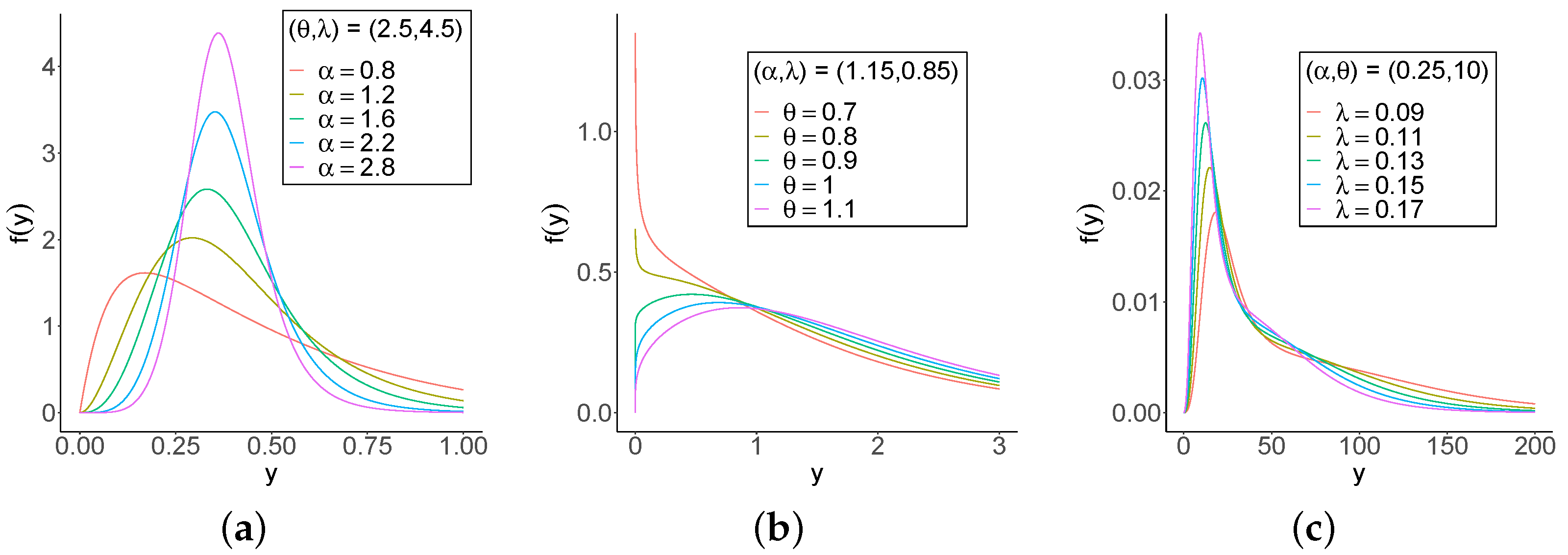
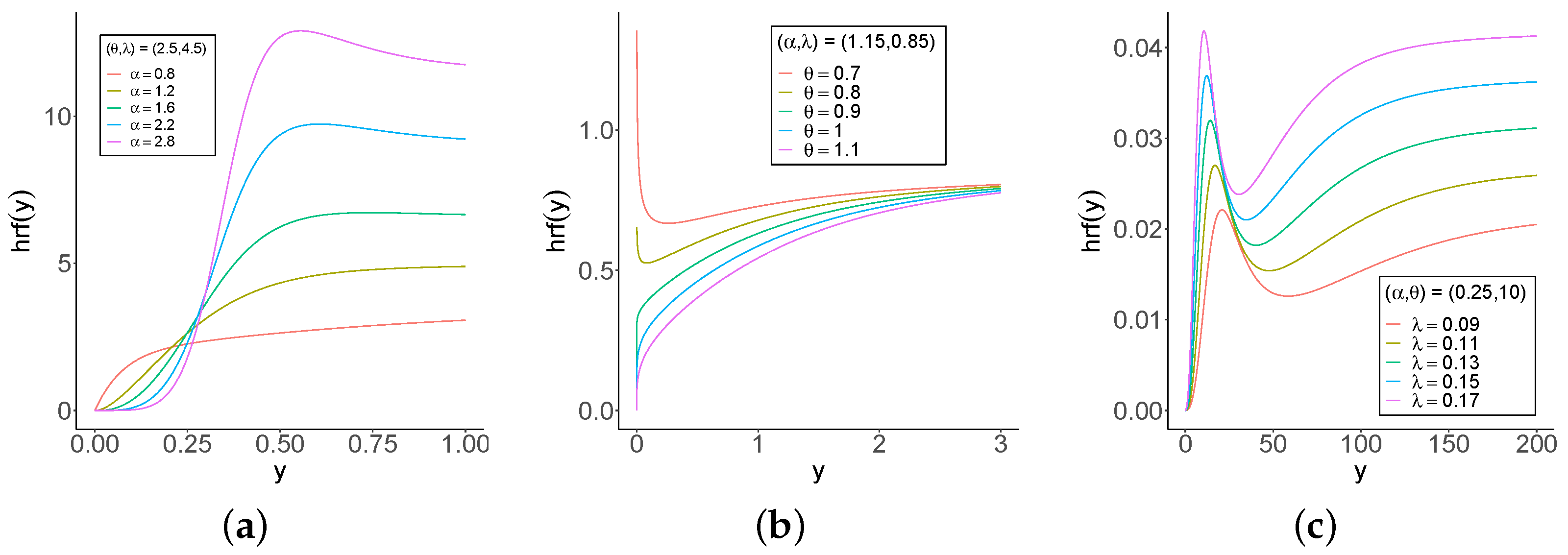
Figure 1 and Figure 2 provide plots of the pdf and hrf of Y for selected parameters. One of the standout characteristic of the GOLLL distribution is its flexibility in generating a vast array of hazard shapes. Figure 2 includes but are not limited to increasing-decreasing-increasing, inverse J-shape, increasing-decreasing, and various other patterns shapes. This exceptional versatility transforms the model into an immensely powerful tool for effectively modeling complex data sets that encompass a wide range of diverse hazard rate patterns.
2.2. Properties
No closed-form mathematical properties of the GOLLL distribution exist. Initially, introducing the EL rv with power parameter and density is done, following from Equations (3) and (4)
Therefore, the pdf of Y can be expressed as a linear representation of EL densities as follows.
2.3. Quantile Function
2.4. Moments
Theorem 1.
The nth ordinary moment of Y is given by
where
2.5. Estimation
Let be a random sample from GOLLL. The log-likelihood function for the parameter vector is given by
For simplicity, let
Then, the components of the score vector, for , are
and
2.6. Simulations
We generate 1000 samples of sizes 50, 100, 200, 400, 800, and 1000, to evaluate the accuracy of the estimators under two scenarios: for scenario 1, and for scenario 2. The average estimates (AEs), biases, and mean square errors (MSEs) are calculated for each sample size, and the findings are reported in Table 2. The measures are
for .
The results indicate that the AEs converge to the true parameters, and the biases and MSEs decay when n increases, thus indicating that the consistency criterion holds.
3. The GOLLL Regression Model
In recent years, new regression models have been proposed to handle various types of data without any transformation. The development accommodates non-normal data and captures the complexity and diversity of real data sets, providing accurate results. Ref. [23] proved the applicability of the utilized family in real engineering data sets. Another work [24] studied the COVID-19 ICU survival times in a Brazilian hospital.
In this situation, new models represent an important step to improve the analysis of different outcomes. Therefore, using the proposed GOLLL distribution, a new regression model is constructed as a tool to investigate any dataset that does not satisfy normality assumptions.
3.1. Definition
The systematic component of the GOLLL regression model takes into account the fact that the parameter in Equation (6) varies across observations () as
where is a twice continuously differentiable log-linear link function, and is the p-dimensional parameter vector associated with the explanatory variables . The components of are assumed to be independent. Therefore, the non-linear function plays the link with the covariates and the new regression model.
Consider a sample of n independent observations . The log-likelihood function for the parameter vector in this regression model has the form
3.2. Simulations of the Regression Model
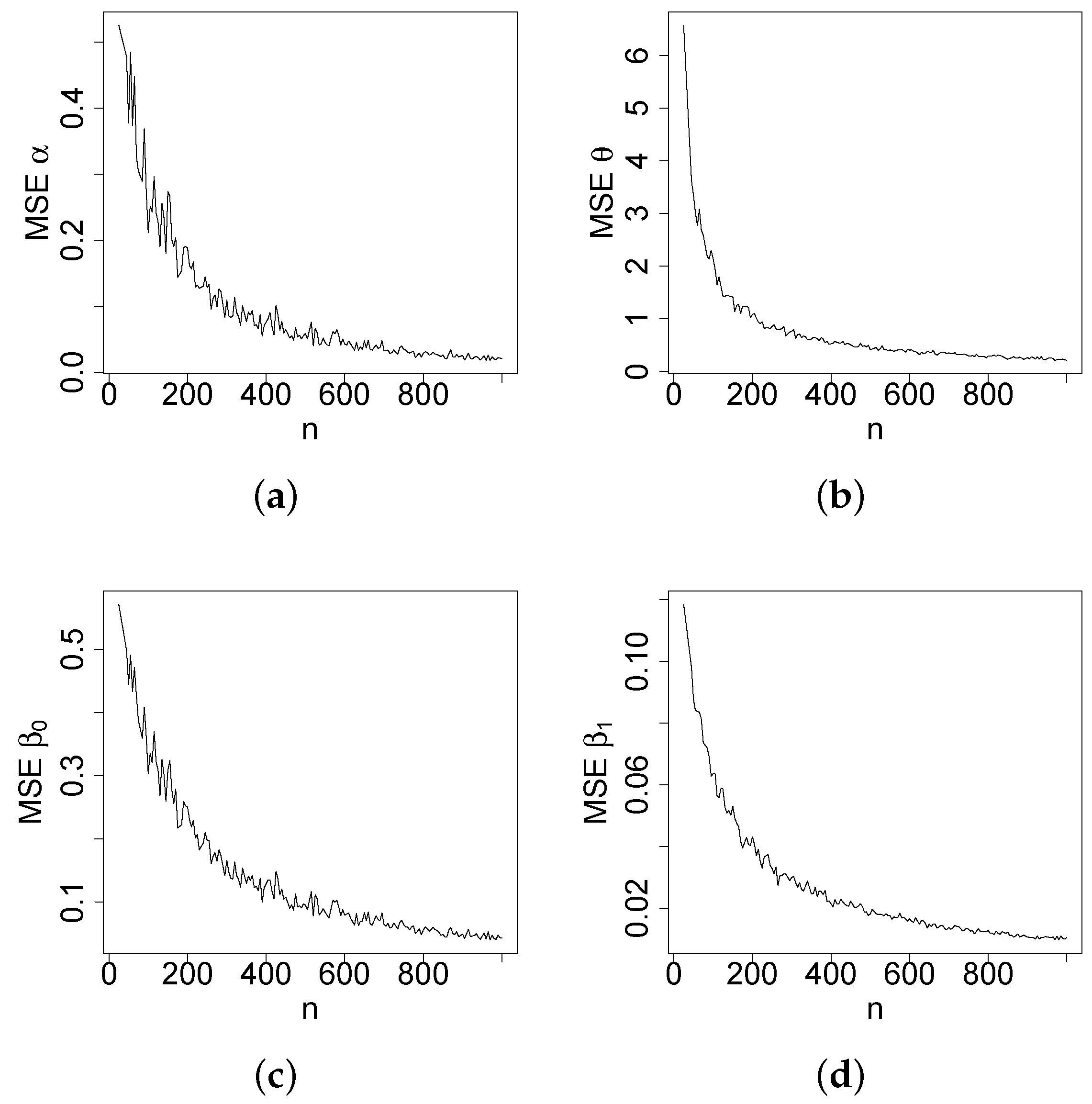
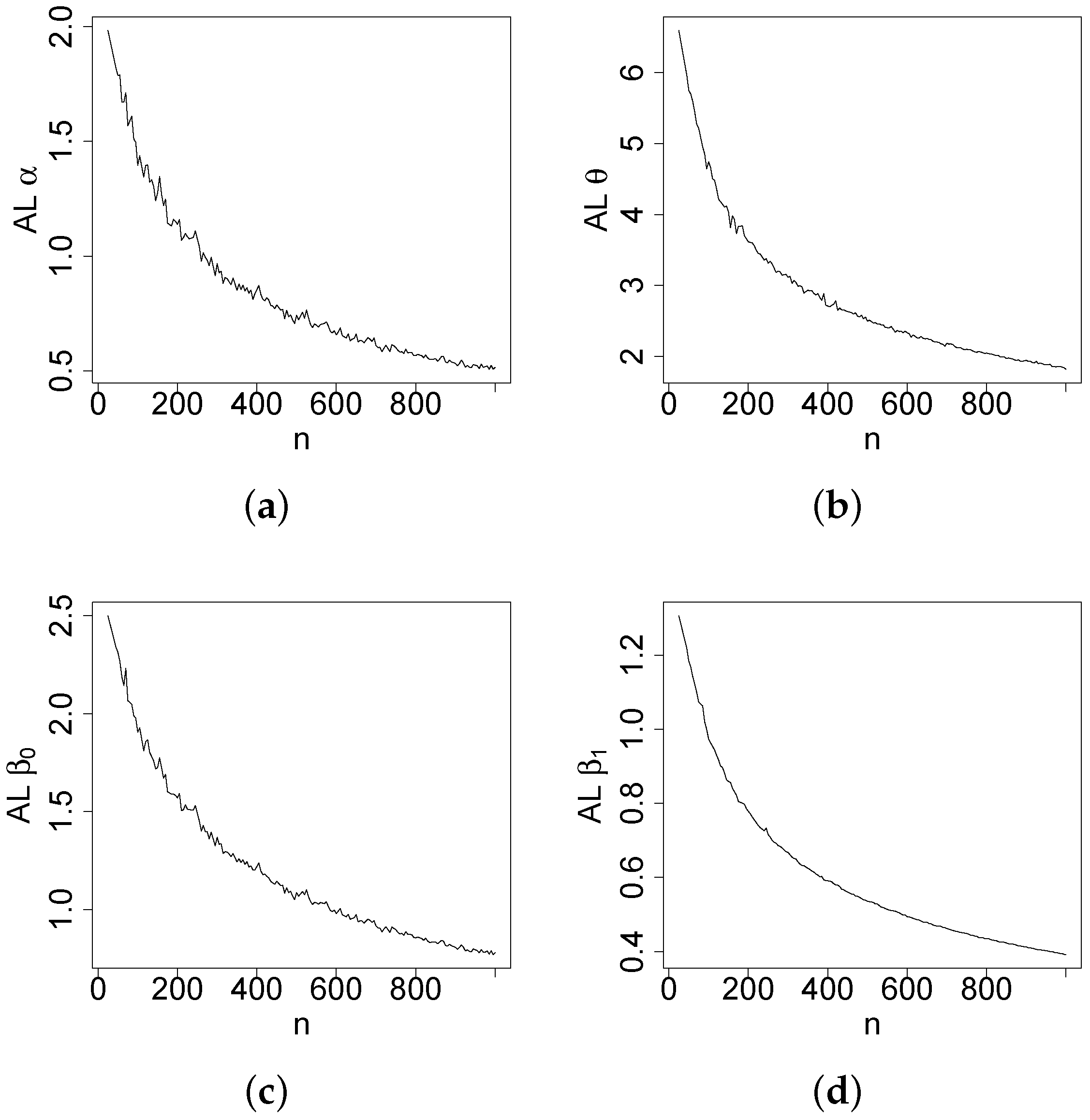
The accuracy of the MLEs in the GOLLL regression model can be assessed using the measures: bias, MSE, estimated average length (AL), and coverage probability (CP). The measures are
and
for .
One-thousand samples of sizes are generated from Equation (8) by setting , , , and . The Monte Carlo simulation provides a versatile approach to analyzing the parameters of the model, enabling researchers to explore the behavior of a distribution under various conditions.
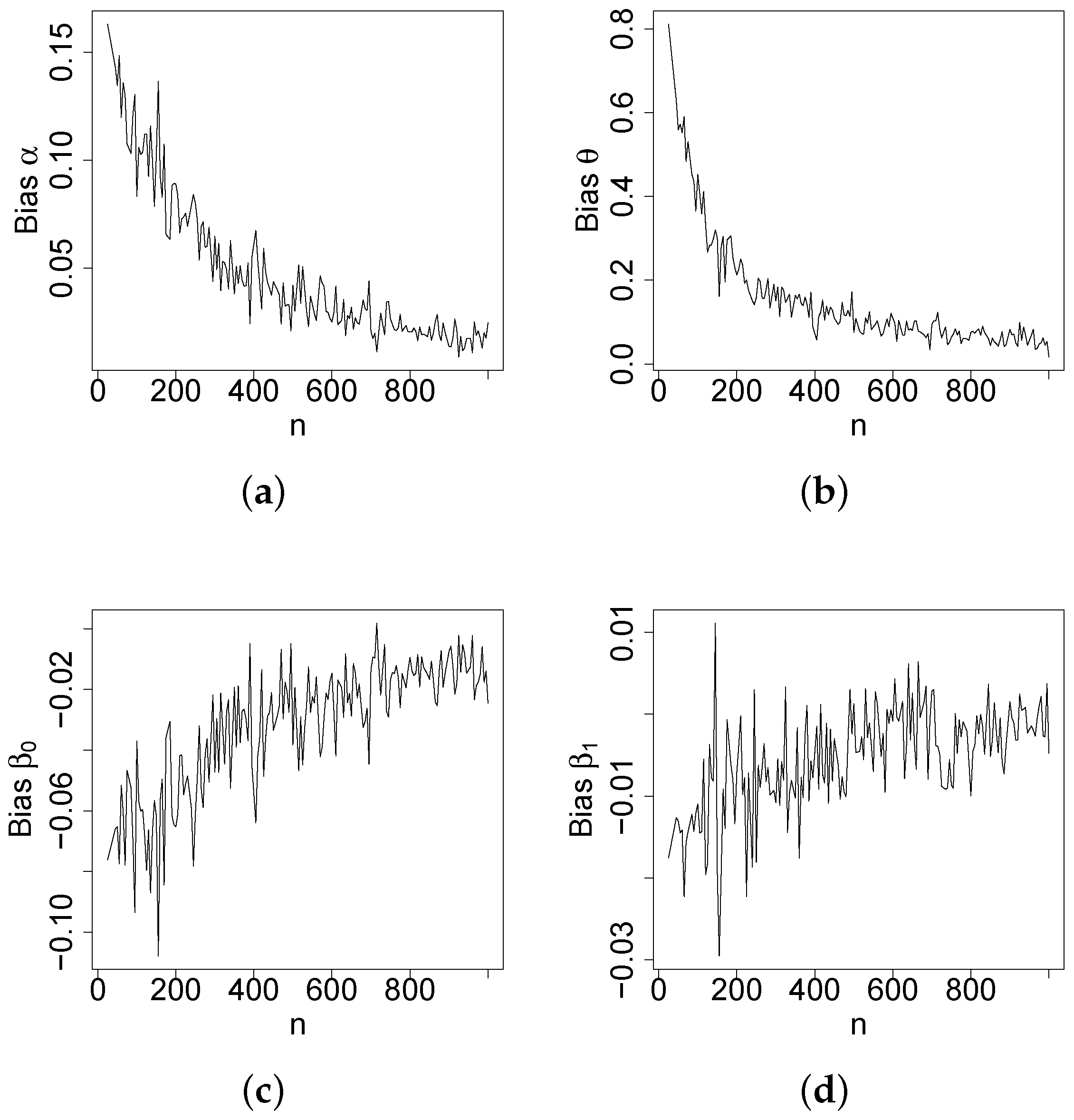
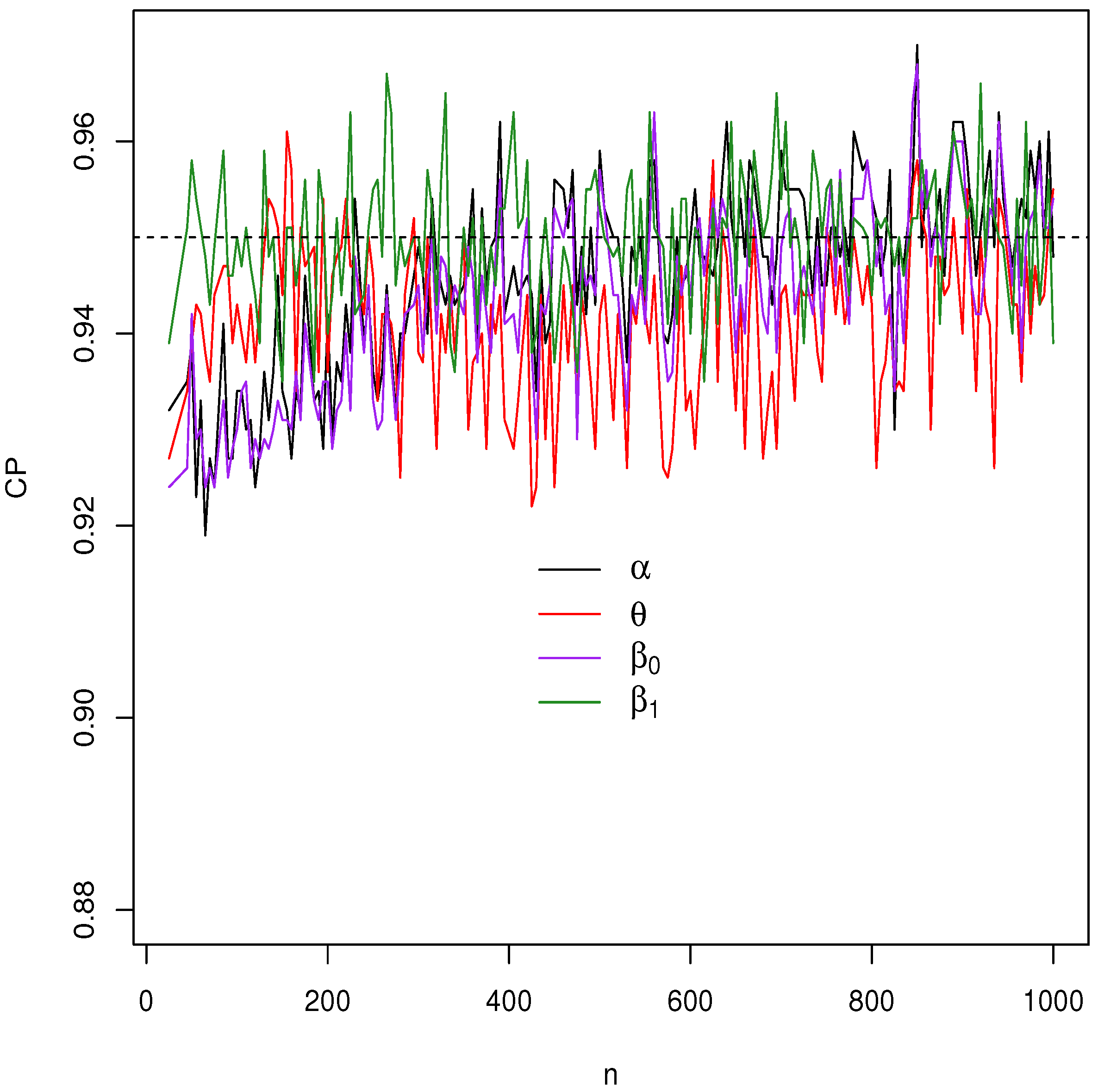
Figure 4, Figure 5, Figure 6 and Figure 7 report how the measure values change with respect to the sample size. The biases, MSEs, and ALs decay toward zero when n increases. Additionally, the CPs approach the true value of if n increases. These findings provide strong evidence of the consistency of the MLEs. The simulation contributed to the reliability and comprehensiveness of the new regression model.
3.3. Model Checking
Diagnostic measures and residual analysis are employed to know if the model accurately represents the data. This involves investigating whether the sample contains any outliers or influential observations that may affect the model’s performance.
Measures based on case deletion are considered in the systematic component to identify influential observations in the regression model
Here, the effect of excluding the ith observation is examined on the parameter estimates. Hence, the log-likelihood function for from model (13) by deleting the ith observation is , and the MLE of the parameter vector is .
The influence of the ith observation is measured by comparing the difference between the estimated parameter and the original MLE . If excluding the ith observation leads to a substantial change in the estimated parameters, then this observation is influential.
A popular influence measure is the generalized Cook distance (GCD), namely
where is the estimated observed information matrix.
Another commonly used influence measure is the likelihood distance (LD), namely
In addition to global influence measures, analyzing residuals can also be an effective way to assess model adequacy and check for incompatibilities with the response distribution. The deviance residuals for the GOLLL regression are
where are the martingale residuals (see [25]), and takes value if the argument is positive/negative.
4. Application
Initially, a comparative analysis of the GOLLL model against some alternative models is conducted. The EL, beta Lindley (BL) [26], Kumaraswamy Lindley (KwL) [27], and gamma-Lindley (GL) [28] distributions are given by
The parameters of all distributions are positive real numbers, and is the Lindley distribution. For all fitted models, the goodness.fit function, using the BFGS method from the AdequacyModel package [29], computes the MLEs (SEs in parentheses). The selection of the best fitted model is based on several well-known measures, including Cramér-von Mises (), Anderson-Darling (), and Kolmogorov-Smirnov (KS) (p-values in parentheses).
4.1. COVID-19 Vaccination Rates on County-Level
To demonstrate the usefulness of the new GOLLL regression model over other competitive models, we provide an application that utilizes county-level COVID-19 vaccination rates in the state of Texas, USA.
The data set refers to 254 percentages of the population in counties with a completed vaccination (aged adjust) to COVID-19 extracted from CDC (https://covid.cdc.gov/covid-data-tracker/#datatracker-home, accessed on 22 February 2023). This data set is used since Texas is the state with the highest number of counties in the US. Further investigation with other data sets (states, countries, and counties) should be addressed to examine the accuracy of the new model.
Additional research has examined the impact of covariates on the COVID-19 vaccination. Ref. [30] analyzed the COVID-19 vaccination coverage associated with social vulnerability and urbanity. Ref. [31] verified the impact of some variables in vaccination coverage and suggested that interventions be undertaken to improve COVID-19 vaccine acceptance and future uptake. The study conducted by [32] utilized machine learning to study the vaccination rate in the USA. The findings provide insights to increase vaccination acceptance and combat the COVID-19 pandemic. Other investigations, Refs. [33,34] demonstrate some predictors for vaccine hesitancy using variables such as social-demographics and comorbidities and conclude a strong association. Therefore, the inclusion of the study variables is based on past research, comparisons, and investigations of possible new associations to aid vaccination campaigns.
The explanatory variables were extracted from County Health Rankings (https://www.countyhealthrankings.org/, data from 2020, accessed on 22 February 2023) are outlined below (for ):
- VR: Population rate with complete primary series of COVID-19 vaccination (response variable);
- HP: Total number of hospitals reporting vaccination;
- PR: Poverty rate (percentage of individuals with income below the poverty line);
- MS: Metropolitan status ( non-metropolitan, metropolitan);
- HR: High school completion rate (proportion of individuals aged 25 and above who have completed high school or its equivalent);
- BA: Broadband access (percentage of households that have access to broadband internet);
- HT: Heart disease rate (percentage of individuals that have chronic heart disease).
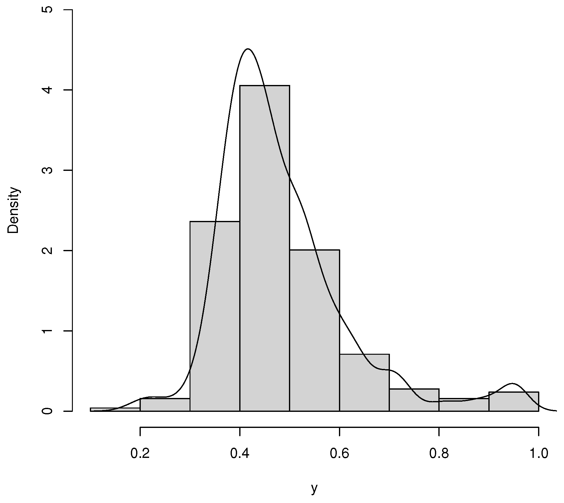
Table 3 reports the descriptive statistics for the data set, and the histogram is given in Figure 8. The average rate of vaccination in counties was 0.483 in the period of the study. The standard deviation is 0.132, which can be explained by the range of 0.189 and 0.950, respectively, the minimum and the maximum. Furthermore, the skewness and kurtosis are positive.
First, the analysis involves modeling only the response variable by fitting the GOLLL, OLLL, EL, L, BL, KwL, and GL distributions. The MLEs, SEs, and the previous statistics (with the p-values of KS) are reported in Table 4 for the fitted distributions to the COVID-19 vaccination rate data. The GOLLL distribution is the most suitable model for the current data based on these measures.
Three LR tests compare the GOLLL distribution with its nested models. The numbers in Table 5 indicate that the inclusion of extra parameters is significant for accurately modeling the current data.
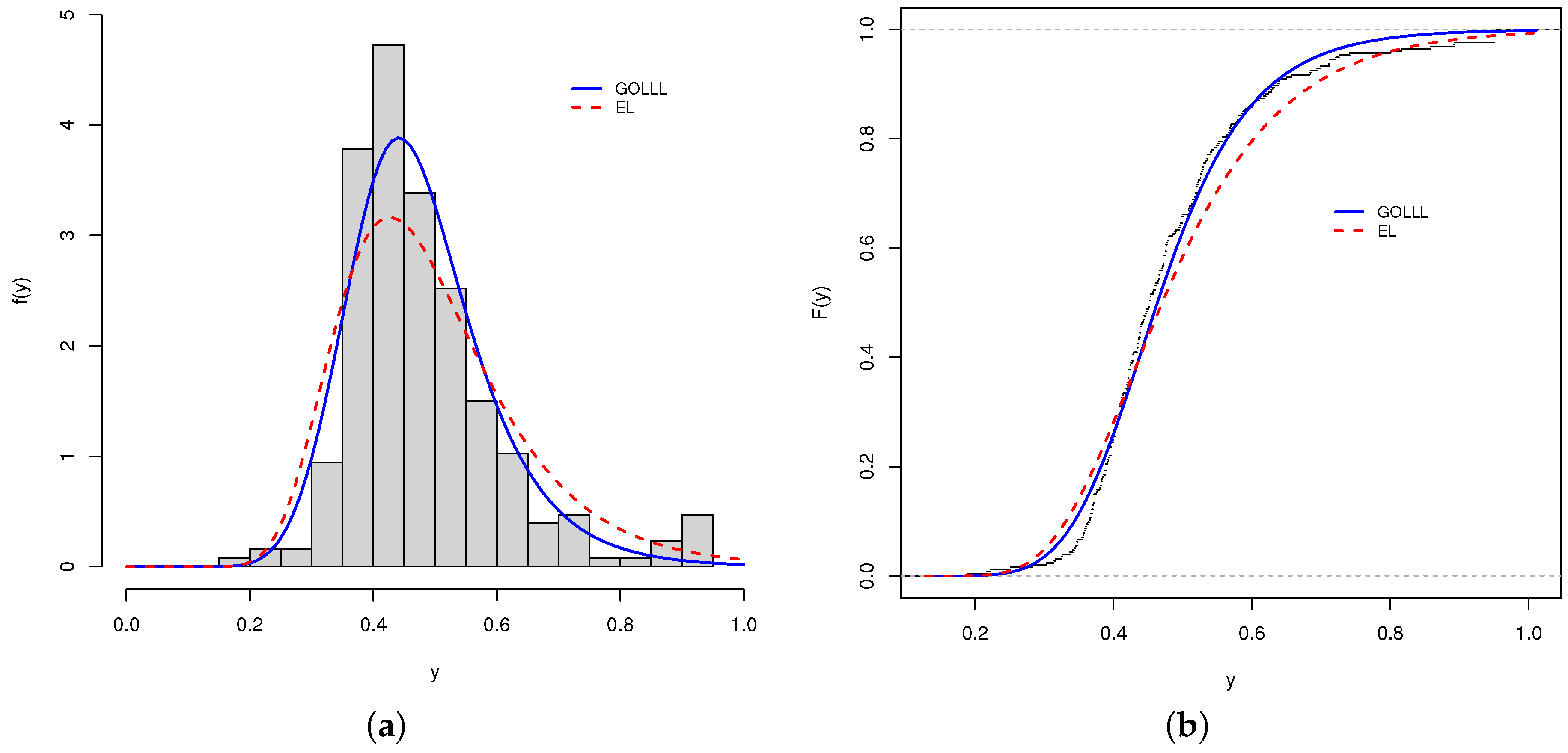
The histogram and fitted densities of the two best models are illustrated in Figure 9a. Further, the estimated cdfs of these models are reported in Figure 9b. Although the model presents a good fit to the current data, it is not enough to know whether the model will be suitable for other datasets at different time or space scales. Future research can test other datasets in different states and at different spatial scales or county levels to investigate the accuracy of the new model.
4.2. Results New Regression
Next, utilizing the new regression model proposed, the systematic component is considered (for )
Table 6 reports the MLEs, SEs, and p-values for the fitted GOLLL regression model to the current data. The numbers support that all six explanatory variables are significant (at the level of ).
4.3. Diagnostic and Residual Analysis
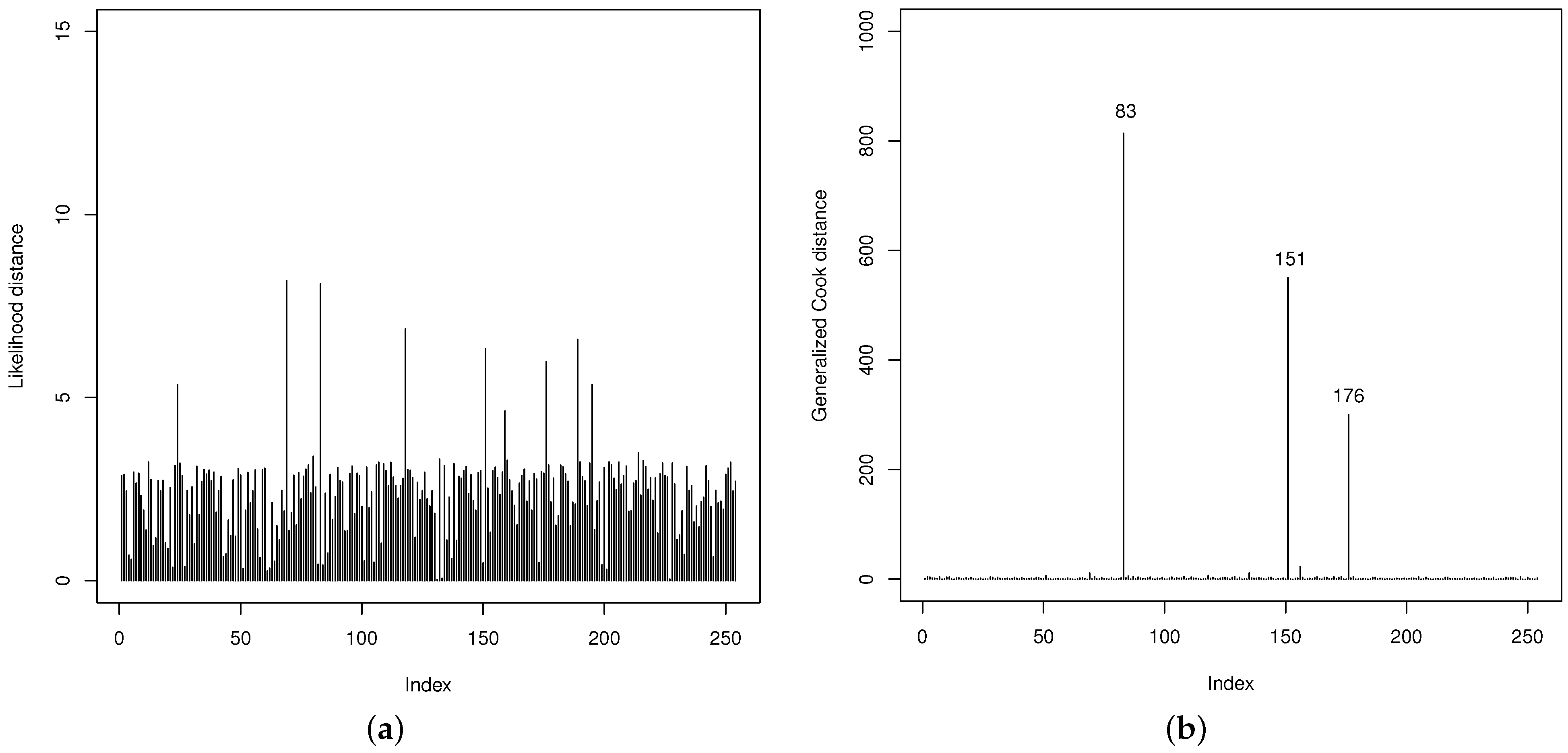
Thereafter, the quality of the fit of the GOLLL regression model is examined. The LD and GCD measures in Figure 10 are useful to identify potentially influential observations. They show that the 83th, 151th, and 176th observations (referring to the counties below) are possibly influential. However, their impacts on the regression model are not particularly significant.
- 83th: Gaines county with VR: , HP: 1, PR: , MS: 0, HR: , BA: and HT: ;
- 151th: Loving county with VR: , HP: 0, PR: , MS: 0, HR: , BA: and HT: ;
- 176th: Newton county with VR: , HP: 0, PR: , MS: 1, HR: , BA: and HT: .
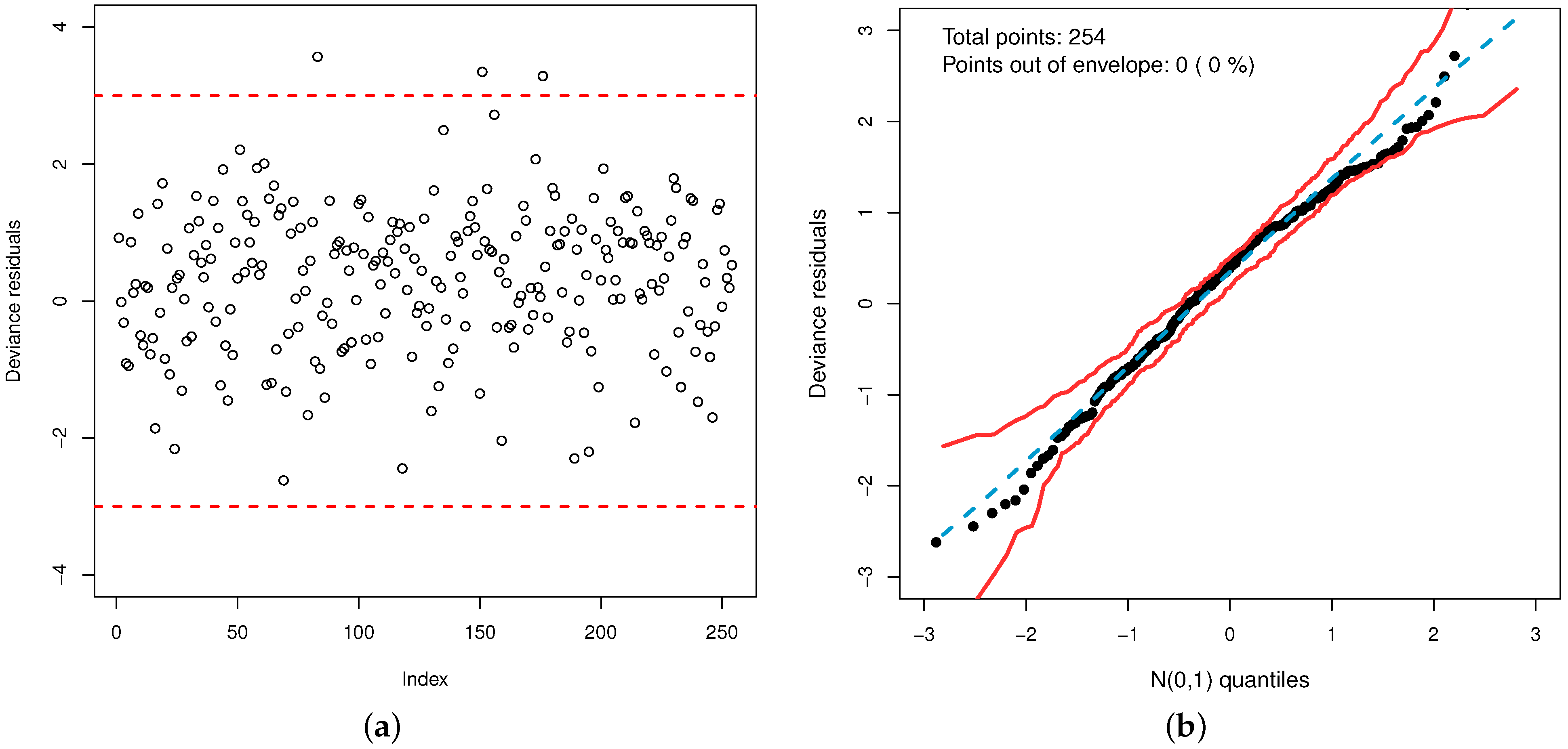
Additionally, the plot of the deviance residuals in Figure 11a shows that they fall randomly within the bands. The normal probability plot with simulated envelope in Figure 11b proves the accuracy of the model to fit the data set. So, the GOLLL regression model provides a good fit.
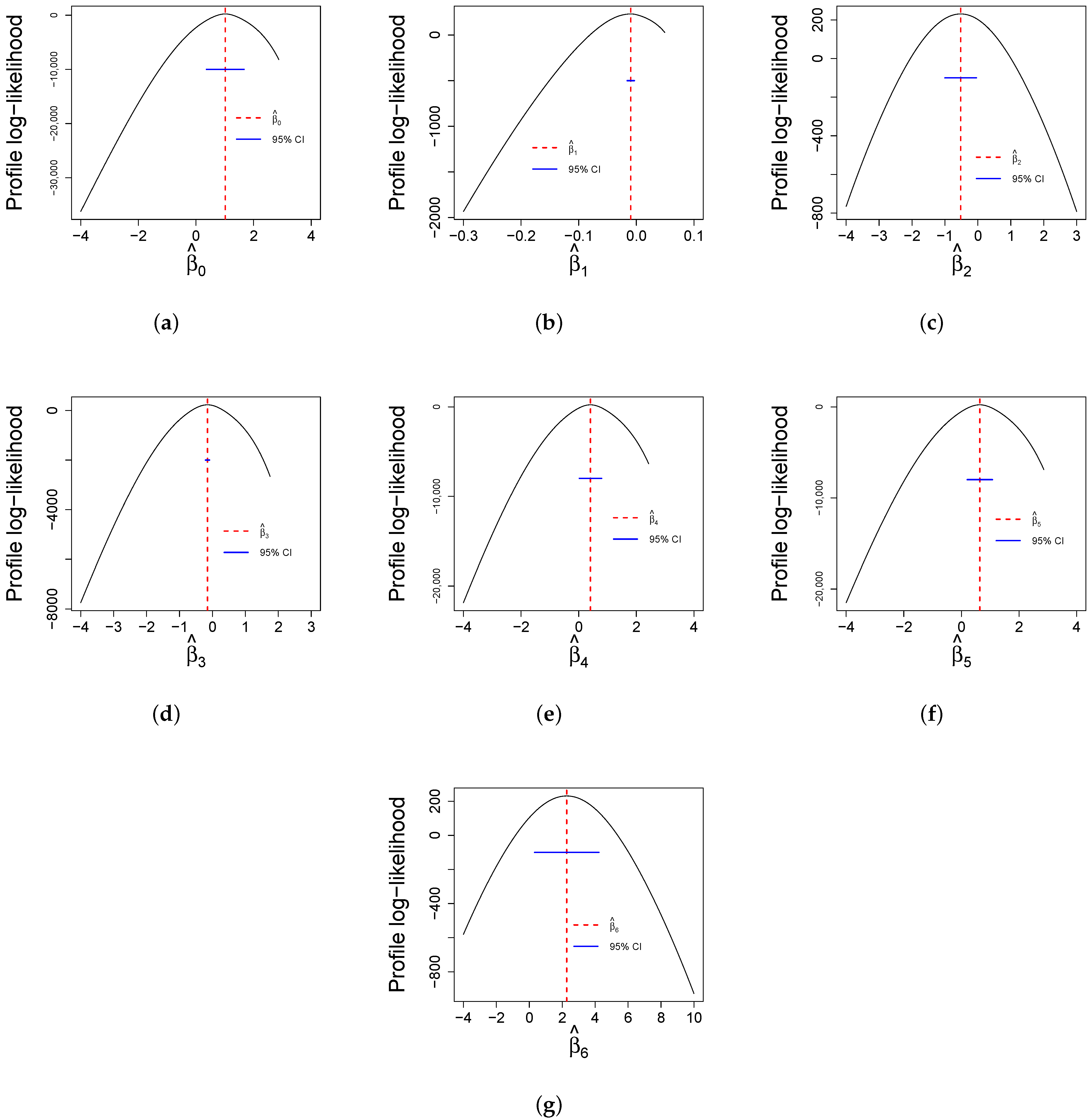
Finally, Figure 12 reports profile log-likelihood plots for the parameters while keeping all other estimates constant. These plots are useful for determining confidence intervals for estimates and the reliability of statistical analyses. The curves of all parameters provide the accuracy and uncertainty associated with parameter estimates.
5. Discussion
The model checks reveal that the GOLLL regression model is suitable to explain the vaccination rates in Texas counties. From the parameter estimates reported in Table 6, the GOLLL regression model becomes
Several facts can be drawn from Equation (18). For each covariate, the study reveals findings that corroborate with other research and indicate the importance of the model for future applications with diverse other vaccination data.
- All variables are statistically significant at a significance level of ;
- The HP variable shows a slight negative estimate, and this negative change is statistically significant;
- The PR variable is significant, and its estimate is negative. COVID-19 increased poverty and inequality worldwide [35,36]. Individuals living in poverty may lack access to reliable transportation, face barriers to accessing healthcare facilities, and have limited resources for paying out-of-pocket costs associated with vaccination [37,38]. The study of [39] revealed the lack of access to the COVID-19 vaccine in the lowest county’s poverty rates across the American state of Illinois. Other study [40] showed a strong negative correlation with poverty and vaccine coverage in the 189 countries’ research. This can result in lower vaccination rates among populations living in poverty, which is supported by data from the proposed model and prior studies;
- The MS variable has a negative estimate, which indicates that the vaccination rate is lower in metropolitan urban areas. The differences in vaccination rates between urban and rural communities are likely driven by various factors, such as differences in access to healthcare resources, vaccine distribution challenges, and mainly vaccine hesitancy [41]. Patterns in COVID-19 vaccination coverage by urbanity are addressed by [30]. It indicated lower vaccination rates in rural than urban areas, which corroborates with the study; Further, the study of [42] presented disparities in COVID-19 vaccination coverage between urban and rural counties and explained it by educational attainment, healthcare infrastructure, and Trump vote share.
- The HR variable is significant with a positive coefficient. Thus, counties with higher high school graduation rates tend to have higher vaccination rates as well, which can be attributed to more access to accurate information regarding vaccines to access better healthcare and vaccination services [43]. Other studies [44,45,46] revealed that high school is a key difference in coverage, access, and hesitancy vaccination;
- The BA variable has a positive estimate, which shows the internet has played a significant role in the COVID-19 vaccination effort. Websites and social media platforms have been used to disseminate information about vaccine availability, eligibility, and safety. The study’s results suggest that counties with greater access to broadcast media have a higher COVID-19 vaccination rate, which highlights the disparities in access to the internet and technology among some communities. This finding is consistent with the research presented in [47]. Alternative studies [48,49], showed that lack of internet access is a barrier to vaccination. In New York City and some counties in North Carolina, the COVID-19 vaccine hesitancy increases if there is difficulty accessing the internet;
- The HT variable has a highly positive estimate. Several studies [50,51,52] have demonstrated the heightened risk of individuals with chronic heart disease contracting and experiencing severe symptoms from COVID-19, as well as increased rates of hospitalization and mortality. For these reasons, many states in the US have implemented targeted outreach efforts to ensure that these populations have access to the vaccine. Hence, the study’s results indicate that counties with high rates of chronic heart disease have a correspondingly higher rate of vaccination. This finding highlights the importance of the government’s focus on prioritizing at-risk populations [53]. Subsequent studies [54,55], illustrated the efficacy and safety of the COVID-19 vaccine based on the presence of comorbidities, including heart disease.
6. Conclusions
This article investigated the factors that explain the COVID-19 vaccination rate using the generalized odd log-logistic Lindley regression model with a shape systematic component. Some mathematical properties of this model were provided, and the maximum likelihood method was used to estimate the parameters. A Monte Carlo simulation evaluated the parameters of the proposed regression model, which revealed the consistency of the estimators and the approach to the nominal level of the coverage probabilities. Diagnostic analysis and deviance residuals proved the suitability of the new model.
The analysis of COVID-19 vaccination rates at the county level in Texas, US, uncovered significant findings. The total number of hospitals reporting vaccination is a slight predictor of vaccination, and it is suggested to be considered in future work for further investigations. Poverty rate and metropolitan status are evidenced in this work as determinants. The first one discussed in [35,36,37,38], among others, reveals the lack of access to the COVID-19 vaccine among individuals living in poverty. The second one examined in [30,41,42] presented disparities in COVID-19 vaccination coverage between urban and rural counties, corroborating with this study. The education level was also identified as a determinant of increasing the vaccination rate. Supporting studies by [43,44,46] indicated that the high school rate is a significant variable in coverage, access, and hesitancy vaccination. Another important variable is broadband access. The internet, supported by websites and social media platforms, disseminates information about vaccines, as suggested by prior studies [47,48,49], and is consistent with the findings of this study. Several studies [50,51,52] worldwide demonstrated how comorbidities influence COVID-19. Countries prioritized the availability of vaccines for people in the risk group, as highlighted in [53]. Subsequent studies [54,55], illustrate findings similar to the current study, including heart disease.
The new model showed that it was more flexible than some competitive models. Hence, it is possible to conclude that the proposed model can provide better insights into the relationship between the explanatory variables and the response variable and serve as an alternative model to evaluate other research. It is recommended to apply the regression model introduced in other states, countries, or cities and verify if the same covariates would be significant in future works.
Author Contributions
Conceptualization, N.S.S.d.C. and G.M.C.; methodology, N.S.S.d.C., M.d.C.S.d.L. and G.M.C.; software, N.S.S.d.C.; validation, N.S.S.d.C., M.d.C.S.d.L. and G.M.C.; formal analysis, N.S.S.d.C., M.d.C.S.d.L. and G.M.C.; investigation, N.S.S.d.C., M.d.C.S.d.L. and G.M.C.; data curation, N.S.S.d.C.; writing—original draft preparation, N.S.S.d.C. and M.d.C.S.d.L.; writing—review and editing, N.S.S.d.C., M.d.C.S.d.L. and G.M.C.; visualization, N.S.S.d.C., M.d.C.S.d.L. and G.M.C.; supervision, N.S.S.d.C., M.d.C.S.d.L. and G.M.C.; project administration, N.S.S.d.C. and M.d.C.S.d.L. All authors have read and agreed to the current version of the manuscript.
Funding
This research received no external funding.
Institutional Review Board Statement
Not applicable.
Informed Consent Statement
Not applicable.
Data Availability Statement
The authors confirm that the data supporting the findings of this study are available within the article.
Conflicts of Interest
The authors declare no conflict of interest.
Abbreviations
The following abbreviations are used in this manuscript:
| Anderson Darling | |
| AE | average estimate |
| AL | average estimate length |
| cdf | cumulative distribution function |
| COVID-19 | corona virus disease 2019 |
| CP | coverage probability |
| L | Lindley distribution |
| EL | exponentiated Lindley distribution |
| GCD | generalized Cook distance |
| GL | gamma-Lindley distribution |
| GOLL-G | generalized odd log-logistic distribution |
| GOLLL | generalized odd log-logistic Lindley distribution |
| KS | Kolmorogov-Sminorv |
| KwE | Kumaraswamy Lindley distribution |
| LD | loglikelihood distance |
| LR | likelihood ratio |
| MLE | maximum likelihood estimate |
| MSE | mean squared error |
| OLLL | odd log-logistic Lindley distribution |
| probability distribution function | |
| T-X | transformer-transformer generator |
| Cramér-von Misses |
References
- Hughes, M.M.; Wang, A.; Grossman, M.K.; Pun, E.; Whiteman, A.; Deng, L.; Hallisey, E.; Sharpe, J.D.; Ussery, E.N.; Stokley, S.; et al. County-Level COVID-19 Vaccination Coverage and Social Vulnerability—United States, 14 December 2020–1 March 2021. In Morbidity and Mortality Weekly Report; Centers for Disease Control and Prevention: Atlanta, GA, USA, 2021; Volume 70, pp. 431–436. [Google Scholar] [CrossRef]
- Razzaghi, H.; Meghani, M.; Pingali, C.; Crane, B.; Naleway, A.; Weintraub, E.; Kenigsberg, T.A.; Lamias, M.J.; Irving, S.A.; Kauffman, T.L.; et al. COVID-19 Vaccination Coverage Among Pregnant Women during Pregnancy—Eight Integrated Health Care Organizations, United States, 14 December 2020–8 May 2021. In Morbidity and Mortality Weekly Report; Centers for Disease Control and Prevention: Atlanta, GA, USA, 2021; Volume 70, pp. 7895–7899. [Google Scholar] [CrossRef]
- Kriss, J.L.; Hung, M.C.; Srivastav, A.; Black, C.L.; Lindley, M.C.; Lee, J.T.; Koppaka, R.; Tsai, Y.; Lu, P.J.; Yankey, D.; et al. COVID-19 Vaccination Coverage, by Race and Ethnicity— National Immunization Survey Adult COVID Module, United States, December 2020–November 2021. In Morbidity and Mortality Weekly Report; Centers for Disease Control and Prevention: Atlanta, GA, USA, 2022; Volume 71, pp. 757–763. [Google Scholar] [CrossRef]
- Albrecht, D. Vaccination, Politics and COVID-19 Impacts. BMC Public Health 2022, 22, 96. [Google Scholar] [CrossRef] [PubMed]
- Reimer, N.K.; Atari, M.; Karimi-Malekabadi, F.; Trager, J.; Kennedy, B.; Graham, J.; Dehghani, M. Moral Values Predict County-Level COVID-19 Vaccination Rates in the United States. Am. Psychol. 2022, 77, 743–759. [Google Scholar] [CrossRef] [PubMed]
- Cordeiro, G.M.; Alizadeh, M.; Ozel, G.; Hosseini, B.; Ortega, E.M.M.; Altun, E. The Generalized Odd Log-Logistic Family of Distributions: Properties, Regression Models and Applications. J. Stat. Comput. Simul. 2017, 87, 908–932. [Google Scholar] [CrossRef]
- Vasconcelos, J.C.S.; Cordeiro, G.M.; Ortega, E.M.M.; Saulo, H. Parametric and partially linear regressions for agricultural economy data. Commun. Stat.—Theory Methods 2022, 1–22. [Google Scholar] [CrossRef]
- Prataviera, F.; Hashimoto, E.M.; Ortega, E.M.M.; Cordeiro, G.M.; Cancho, V.G.; Vila, R. A new flexible regression model with application to recovery probability COVID-19 patients. J. Appl. Stat. 2023, 1–19. [Google Scholar] [CrossRef]
- Tarvirdizade, B. The Lomax-Lindley Distribution: Properties and Applications to Lifetime Data. Commun. Fac. Sci. Univ. Ank. Ser. Math. Stat. 2021, 70, 965–983. [Google Scholar] [CrossRef]
- Karakaya, K.; Korkmaz, M.C.; Chesneau, C.; Hamedani, G.G. A New Alternative Unit-Lindley Distribution with Increasing Failure Rate. Sci. Iran. 2022, in press. [Google Scholar] [CrossRef]
- Hameed, A.N.; Saieed, H.A.J. Construction of Marshall-Olkin Lindley Distribution with Application. In Proceedings of the 8th International Conference on Contemporary Information Technology and Mathematics (ICCITM), Mosul, Iraq, 31 August–1 September 2022; pp. 437–441. [Google Scholar] [CrossRef]
- Coşkun, K.U.Ş.; Korkmaz, M.Ç.; Kinaci, İ.; Karakaya, K.; AkdoĞan, Y. Modified-Lindley Distribution and its Applications to the Real Data. Commun. Fac. Sci. Univ. Ank. Ser. Math. Stat. 2022, 71, 252–272. [Google Scholar] [CrossRef]
- Alzaatreh, A.; Lee, C.; Famoye, F. A New Method for Generating Families of Continuous Distributions. Metron 2013, 71, 63–79. [Google Scholar] [CrossRef]
- Gleaton, J.U.; Lynch, J.D. Properties of Generalized Log-Logistic Families of Lifetime Distributions. J. Probab. Stat. Sci. 2006, 4, 51–64. Available online: https://www.researchgate.net/publication/283595537_Properties_of_generalized_log-logistic_families_of_lifetime_distributions (accessed on 21 November 2023).
- Gupta, R.C.; Gupta, R.D. Proportional Reversed Hazard Rate Model and its Applications. J. Stat. Plan. Inference 2007, 137, 3525–3536. [Google Scholar] [CrossRef]
- Ozel, G.; Alizadeh, M.; Cakmakyapan, S.; Hamedani, G.G.; Ortega, E.M.M.; Cancho, V.G. The Odd Log-Logistic Lindley Poisson Model for Lifetime Data. Commun.-Stat.-Simul. Comput. 2017, 46, 331–359. [Google Scholar] [CrossRef]
- Nadarajah, S.; Bakouch, H.S.; Tahmasbi, R. A Generalized Lindley Distribution. Sankhya B 2011, 73, 331–359. [Google Scholar] [CrossRef]
- Lindley, D.V. Fiducial Distributions and Bayes Theorem. J. R. Stat. Soc. Ser. B 1958, 20, 102–107. Available online: http://www.jstor.org/stable/2983909 (accessed on 21 November 2023). [CrossRef]
- Galton, F. Enquiries into Human Faculty and Its Development; Macmillan & Company: London, UK, 1883; Available online: https://psycnet.apa.org/doi/10.1037/14178-000 (accessed on 21 November 2023).
- Moors, J.J.A. A Quantile Alternative for Kurtosis. J. R. Stat. Soc. Ser. D 1988, 37, 25–32. [Google Scholar] [CrossRef]
- Ranjbar, V.; Alizadeh, M.; Altun, E. Extended Generalized Lindley Distribution: Properties and Applications. J. Math. Ext. 2019, 13, 117–142. Available online: https://ijmex.com/index.php/ijmex/article/viewFile/755/377 (accessed on 21 November 2023).
- R Core Team. R Core Team: A Language and Environment for Statistical Computing; R Foundation for Statistical Computing: Vienna, Austria, 2023. [Google Scholar]
- Prataviera, F.; Ortega, E.M.; Cordeiro, G.M. A New Bimodal Maxwell Regression Model with Engineering Applications. Appl. Math. Inf. Sci. 2020, 14, 817–831. [Google Scholar] [CrossRef]
- da Costa, N.S.; Cordeiro, G.M. A New Normal Regression with Medical Applications. Appl. Math. Inf. Sci. 2023, 17, 309–322. [Google Scholar] [CrossRef]
- Pregibon, D. Logistic Regression Diagnostics. Ann. Stat. 1981, 9, 705–724. [Google Scholar] [CrossRef]
- Merovci, F.; Sharma, V.K. The beta-Lindley Distribution: Properties and Applications. J. Appl. Math. 2014, 2014, 198951. [Google Scholar] [CrossRef]
- Çakmakyapan, S.; Kadilar, G.O. A New Customer Lifetime Duration Distribution: The Kumaraswamy Lindley Distribution. Int. J. Trade Econ. Financ. 2014, 5, 4–12. [Google Scholar] [CrossRef]
- Zeghdoudi, H.; Nedjar, S. Gamma Lindley Distribution and its Application. J. Appl. Probab. Stat. 2016, 11, 129–138. [Google Scholar]
- Marinho, P.R.D.; Silva, R.B.; Bourguignon, M.; Cordeiro, G.M.; Nadarajah, S. AdequacyModel: An R package for probability distributions and general purpose optimization. PLoS ONE 2019, 14, e0221487. [Google Scholar] [CrossRef] [PubMed]
- Barry, V.; Dasgupta, S.; Weller, D.L.; Kriss, J.L.; Cadwell, B.L.; Rose, C.; Pingali, C.; Musial, T.; Sharpe, J.D.; Flores, S.A.; et al. Patterns in COVID-19 Vaccination Coverage, by Social Vulnerability and Urbanicity—United States, 14 December 2020–1 May 2021. MMWR Morb. Mortal. Wkly. Rep. 2021, 70, 818–824. [Google Scholar] [CrossRef]
- Wang, Q.; Yang, L.; Jin, H.; Lin, L. Vaccination against COVID-19: A systematic review and meta-analysis of acceptability and its predictors. Prev. Med. 2021, 150, 106694. [Google Scholar] [CrossRef] [PubMed]
- Osman, S.H.I.; Sabit, A. Predictors of COVID-19 vaccination rate in USA: A machine learning approach. Mach. Learn. Appl. 2022, 10, 100408. [Google Scholar] [CrossRef] [PubMed]
- Muthukrishnan, J.; Vardhan, V.; Mangalesh, S.; Koley, M.; Shankar, S.; Yadav, K.; Khera, A. Vaccination status and COVID-19 related mortality: A hospital based cross sectional study. Med. J. Armed Forces India 2021, 77, S278–S282. [Google Scholar] [CrossRef] [PubMed]
- Savoia, E.; Piltch-Loeb, R.; Goldberg, B.; Miller-Idriss, C.; Hughes, B.; Montrond, A.; Kayyem, J.; Testa, M.A. Predictors of COVID-19 Vaccine Hesitancy: Socio-Demographics, Co-Morbidity, and Past Experience of Racial Discrimination. Vaccines 2021, 9, 767. [Google Scholar] [CrossRef]
- Buheji, M.; da Costa Cunha, K.; Beka, G.; Mavric, B.; De Souza, Y.L.; da Costa Silva, S.S.; Yein, T.C. The Extent of COVID-19 Pandemic Socio-Economic Impact on Global Poverty. A Global Integrative Multidisciplinary Review. Am. J. Econ. 2020, 10, 213–224. [Google Scholar] [CrossRef]
- Deaton, A. COVID-19 and Global Income Inequality. LSE Public Policy Rev. 2021, 1, 1. [Google Scholar] [CrossRef]
- Hyder, A.A.; Hyder, M.A.; Nasir, K.; Ndebele, P. Inequitable COVID-19 Vaccine Distribution and its Effects. Bull. World Health Organ. 2021, 99, 406A. [Google Scholar] [CrossRef] [PubMed]
- Parolin, Z.; Lee, E.K. The role of poverty and racial discrimination in exacerbating the health consequences of COVID-19. Lancet Reg. Health 2022, 7, 100178. [Google Scholar] [CrossRef] [PubMed]
- Liao, T.F. Social and economic inequality in coronavirus disease 2019 vaccination coverage across Illinois counties. Sci. Rep. 2021, 11, 18443. [Google Scholar] [CrossRef] [PubMed]
- de Oliveira, B.R.B.; da Penha Sobral, A.I.G.; Marinho, M.L.M.; Sobral, M.F.F.; de Souza Melo, A.; Duarte, G.B. Determinants of access to the SARS-CoV-2 vaccine: A preliminary approach. Int. J. Equity Health 2021, 20, 183. [Google Scholar] [CrossRef] [PubMed]
- Murthy, B.P.; Sterrett, N.; Weller, D.; Zell, E.; Reynolds, L.; Toblin, R.L.; Harris, L.Q. A Disparities in COVID-19 vaccination coverage between urban and rural counties—United States. Morb. Mortal. Wkly. Rep. 2015, 70, 759–764. [Google Scholar] [CrossRef] [PubMed]
- Sun, Y.; Monnat, S.M. Rural-urban and within-rural differences in COVID-19 vaccination rates. J. Rural. Health 2022, 38, 916–922. [Google Scholar] [CrossRef] [PubMed]
- Khairat, S.; Zou, B.; Adler-Milstein, J. Factors and Reasons Associated with Low COVID-19 Vaccine Uptake among Highly Hesitant Communities in the US. Am. J. Infect. Control 2022, 50, 262–267. [Google Scholar] [CrossRef]
- Malik, A.A.; McFadden, S.M.; Elharake, J.; Omer, S.B. Determinants of COVID-19 vaccine acceptance in the US. EClinicalMedicine 2020, 26, 100495. [Google Scholar] [CrossRef]
- Agarwal, R.; Dugas, M.; Ramaprasad, J.; Luo, J.; Li, G.; Gao, G. Socioeconomic privilege and political ideology are associated with racial disparity in COVID-19 vaccination. Proc. Natl. Acad. Sci. USA 2021, 118, e2107873118. [Google Scholar] [CrossRef]
- Coughenour, C.; Gakh, M.; Sharma, M.; Labus, B.; Chien, L.C. Assessing determinants of COVID-19 vaccine hesitancy in Nevada. Health Secur. 2021, 19, 592–604. [Google Scholar] [CrossRef]
- Goel, R.K.; Nelson, M.A. COVID-19 Internet Vaccination Information and Vaccine Administration: Evidence from the United States. J. Econ. Financ. 2021, 45, 716–734. [Google Scholar] [CrossRef]
- Michaels, I.H.; Pirani, S.J.; Carrascal, A. Disparities in Internet Access and COVID-19 Vaccination in New York City. Prev. Chronic Dis. 2021, 18, 210143. [Google Scholar] [CrossRef] [PubMed]
- Doherty, I.A.; Pilkington, W.; Brown, L.; Billings, V.; Hoffler, U.; Kumar, D. COVID-19 vaccine hesitancy in underserved communities of North Carolina. PLoS ONE 2021, 16, e0248542. [Google Scholar] [CrossRef]
- Clerkin, K.J.; Fried, J.A.; Raikhelkar, J.; Sayer, G.; Griffin, J.M.; Masoumi, A.; Jain, S.S.; Burkhoff, D.; Kumaraiah, D.; Rabbani, L. COVID-19 and Cardiovascular Disease. Circulation 2010, 141, 1648–1655. [Google Scholar] [CrossRef]
- Zhang, J.; Dong, X.; Cao, Y.; Yuan, Y.; Yang, Y.; Yan, Y.; Akdis, C.A.; Gao, Y. Associations of 4 Geographic Social Vulnerability Indices with US COVID-19 Incidence and Mortalit. Allergy 2020, 75, 1730–1741. [Google Scholar] [CrossRef] [PubMed]
- Guan, W.; Liang, W.; Zhao, Y.; Liang, H.; Chen, Z.; Li, Y.; Liu, X.; Chen, R.; Tang, C.; Wang, T. Comorbidity and its Impact on 1590 Patients with COVID-19 in China: A Nationwide Analysis. Eur. Respir. J. 2020, 55, 2000547. [Google Scholar] [CrossRef]
- Osuagwu, U.L.; Langsi, R.; Ovenseri-Ogbomo, G.; Mashige, K.P.; Abu, E.K.; Envuladu, E.A.; Agho, K.E. Analysis of Perception, Reasons, and Mtivations for COVID-19 Vaccination in People with Diabetes Across Sub-Saharan Africa: A Mixed-Method Approach. Int. J. Environ. Res. Public Health 2022, 19, 7875. [Google Scholar] [CrossRef]
- Choi, W.S.; Cheong, H.J. COVID-19 Vaccination for People with Comorbidities. Infect. Chemother. 2021, 153, 155–158. [Google Scholar] [CrossRef]
- Yelin, I.; Katz, R.; Herzel, E.; Berman-Zilberstein, T.; Ben-Tov, A.; Kuint, J.; Kishony, R. Associations of the BNT162b2 COVID-19 vaccine effectiveness with patient age and comorbidities. Medrxiv 2021, 3. [Google Scholar] [CrossRef]
Figure 1.
GOLLL pdf. (a) Varying , fixed and (b) Varying , fixed and . (c) Varying , fixed and .

Figure 2.
GOLLL hrf (a) Varying , fixed and (b) Varying , fixed and . (c) Varying , fixed and .

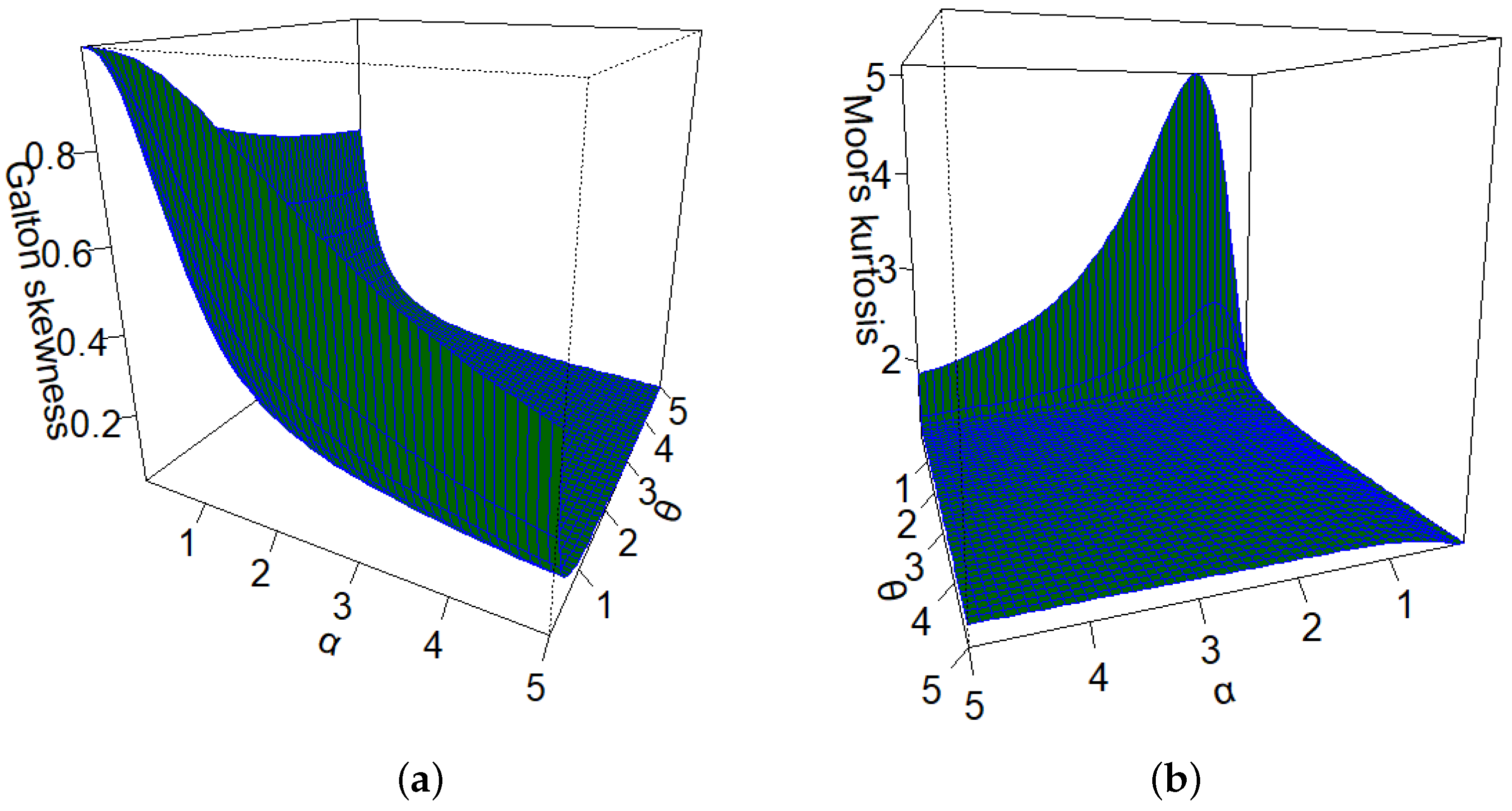
Figure 3.
(a) Galton’s skewness. (b) Moors’ kurtosis.

Figure 4.
Plots of the biases of the estimates. (a) . (b) . (c) . (d) .

Figure 5.
Plots of the MSEs of the estimates. (a) . (b) . (c) . (d) .

Figure 6.
Plots of the ALs of the estimates. (a) . (b) . (c) . (d) .

Figure 7.
Plots of the CPs of the estimates.

Figure 8.
Histogram and empirical density of COVID-19 vaccination rates.

Figure 9.
Fitted models. (a) Histogram and estimated pdfs. (b) Empirical and estimated cdfs.

Figure 10.
The GOLLL regression. (a) LD. (b) GCD.

Figure 11.
(a) Deviance residual plot (Circles—residuals and Lines—Bands of three standard deviations). (b) Normal probability plot of ’s with envelope.
Figure 11.
(a) Deviance residual plot (Circles—residuals and Lines—Bands of three standard deviations). (b) Normal probability plot of ’s with envelope.

Figure 12.
Profile log-likelihood functions from the fitted GOLLL regression model to COVID-19 data with confidence intervals. Parameters: (a) . (b) . (c) . (d) . (e) . (f) . (g) .
Figure 12.
Profile log-likelihood functions from the fitted GOLLL regression model to COVID-19 data with confidence intervals. Parameters: (a) . (b) . (c) . (d) . (e) . (f) . (g) .


Table 1.
Sub-models.
| Sub-Model | ||
|---|---|---|
| - | 1 | Generalized log-logistic family [14] |
| 1 | - | Proportional reversed hazard rate family [15] |
| 1 | 1 | Baseline |
Table 2.
Simulation.
| Scenario 1 | |||||||||
|---|---|---|---|---|---|---|---|---|---|
| Par | n = 50 | n = 100 | n = 200 | ||||||
| AE | Bias | MSE | AE | Bias | MSE | AE | Bias | MSE | |
| 0.561 | 0.061 | 0.126 | 0.507 | 0.007 | 0.010 | 0.538 | 0.0038 | 0.061 | |
| 1.019 | 0.269 | 0.588 | 0.778 | 0.028 | 0.035 | 0.883 | 0.133 | 0.238 | |
| 1.529 | 0.279 | 0.919 | 1.280 | 0.030 | 0.074 | 1.389 | 0.139 | 0.420 | |
| Par | n = 400 | n = 800 | n = 1000 | ||||||
| AE | Bias | MSE | AE | Bias | MSE | AE | Bias | MSE | |
| 0.515 | 0.015 | 0.025 | 0.560 | 0.060 | 0.212 | 0.511 | 0.011 | 0.013 | |
| 0.822 | 0.072 | 0.099 | 1.280 | 0.530 | 1.467 | 0.778 | 0.028 | 0.043 | |
| 1.328 | 0.078 | 0.194 | 1.774 | 0.524 | 1.719 | 1.278 | 0.028 | 0.087 | |
| Scenario 2 | |||||||||
| Par | n = 50 | n = 100 | n = 200 | ||||||
| AE | Bias | MSE | AE | Bias | MSE | AE | Bias | MSE | |
| 1.466 | 0.016 | 0.534 | 1.457 | 0.007 | 0.040 | 1.453 | 0.003 | 0.249 | |
| 0.393 | 0.143 | 0.214 | 0.255 | 0.005 | 0.002 | 0.308 | 0.058 | 0.047 | |
| 1.694 | 0.744 | 4.627 | 0.981 | 0.031 | 0.066 | 1.282 | 0.332 | 1.280 | |
| Par | n = 400 | n = 800 | n = 1000 | ||||||
| AE | Bias | MSE | AE | Bias | MSE | AE | Bias | MSE | |
| 1.431 | −0.019 | 0.097 | 1.546 | 0.096 | 1.399 | 1.444 | −0.006 | 0.047 | |
| 0.271 | 0.021 | 0.007 | 0.608 | 0.358 | 0.855 | 0.258 | 0.008 | 0.002 | |
| 1.087 | 0.137 | 0.251 | 2.556 | 1.606 | 13.543 | 1.007 | 0.057 | 0.085 | |
Table 3.
Descriptive statistics.
| Statistics | |||||||
|---|---|---|---|---|---|---|---|
| Variable | Mean | Median | SD | Skewness | Kurtosis | Min. | Max. |
| VR | 0.483 | 0.452 | 0.132 | - 1.485 | 6.021 | 0.189 | 0.950 |
| HP | 1.717 | 1.000 | 4.282 | - 6.666 | 56.447 | 0.000 | 45.000 |
| PR | 0.161 | 0.152 | 0.061 | -1.022 | 4.878 | 0.026 | 0.395 |
| HR | 0.818 | 0.830 | 0.085 | −2.056 | 12.509 | 0.220 | 0.970 |
| BA | 0.769 | 0.770 | 0.084 | −0.388 | 3.301 | 0.480 | 0.970 |
| HT | 0.082 | 0.082 | 0.017 | -0.248 | 2.906 | 0.045 | 0.134 |
Table 4.
Findings from the fitted models.
| Model | Parameters | KS | ||||
|---|---|---|---|---|---|---|
| 1.490 | 18.003 | 7.814 | 0.306 | 2.076 | 0.059 | |
| (0.0002) | (0.0001) | (0.0003) | (0.338) | |||
| OLLL() | 4.985 | 1 | 2.084 | 0.444 | 2.774 | 0.067 |
| (0.264) | (-) | (0.025) | (0.202) | |||
| EL() | 1 | 35.255 | 9.127 | 0.321 | 2.275 | 0.097 |
| (-) | (5.861) | (0.400) | (0.015) | |||
| L() | 1 | 1 | 2.640 | 0.702 | 4.480 | 0.450 |
| (-) | (-) | (0.136) | (<0.0001) | |||
| BL() | 30.015 | 1.810 | 7.245 | 0.397 | 2.696 | 0.079 |
| (7.324) | (0.503) | (1.155) | (0.082) | |||
| KwL() | 20.113 | 2.156 | 6.676 | 0.493 | 3.235 | 0.081 |
| (4.372) | (0.514) | (0.764) | (0.069) | |||
| GL() | 7.807 | 0.005 | 0.307 | 0.793 | 5.013 | 0.126 |
| (0.751) | (<0.001) | (0.022) | (<0.0001) | |||
Table 5.
LR tests.
| Models | Statistic w | p-Value |
|---|---|---|
| GOLLL vs. OLLL | 5.194 | <0.0227 |
| GOLLL vs. EL | 15.127 | <0.0001 |
| GOLLL vs. L | 498.805 | <0.0001 |
Table 6.
Fitted GOLLL regression to COVID-19 vaccination rates.
| Parameter | Estimate | SE | p-Value |
|---|---|---|---|
| 0.347 | |||
| HP | −0.010 | 0.003 | |
| PR | −0.524 | 0.243 | |
| MS | −0.149 | 0.031 | 0.001 |
| HR | 0.197 | ||
| BA | 0.223 | ||
| HT | 0.995 |
Disclaimer/Publisher’s Note: The statements, opinions and data contained in all publications are solely those of the individual author(s) and contributor(s) and not of MDPI and/or the editor(s). MDPI and/or the editor(s) disclaim responsibility for any injury to people or property resulting from any ideas, methods, instructions or products referred to in the content. |
© 2023 by the authors. Licensee MDPI, Basel, Switzerland. This article is an open access article distributed under the terms and conditions of the Creative Commons Attribution (CC BY) license (https://creativecommons.org/licenses/by/4.0/).
Share and Cite
MDPI and ACS Style
da Costa, N.S.S.; de Lima, M.d.C.S.; Cordeiro, G.M. Analyzing County-Level COVID-19 Vaccination Rates in Texas: A New Lindley Regression Model. COVID 2023, 3, 1761-1780. https://doi.org/10.3390/covid3120122
AMA Style
da Costa NSS, de Lima MdCS, Cordeiro GM. Analyzing County-Level COVID-19 Vaccination Rates in Texas: A New Lindley Regression Model. COVID. 2023; 3(12):1761-1780. https://doi.org/10.3390/covid3120122
Chicago/Turabian Styleda Costa, Nicollas S. S., Maria do Carmo S. de Lima, and Gauss M. Cordeiro. 2023. "Analyzing County-Level COVID-19 Vaccination Rates in Texas: A New Lindley Regression Model" COVID 3, no. 12: 1761-1780. https://doi.org/10.3390/covid3120122