Article

Assessing Land Use/Land Cover Changes and Urban Heat Island Intensification: A Case Study of Kamrup Metropolitan District, Northeast India (2000–2032)

1
Centre for Climate Change and Water Research, Suresh Gyan Vihar University, Jaipur 302017, India
2
Centre for Sustainable Development, Suresh Gyan Vihar University, Jaipur 302017, India
3
Graduate School of Agricultural and Life Sciences, The University of Tokyo, Tokyo 113-8654, Japan
4
Institute for Global Environmental Strategies, Hayama 240-0115, Japan
5
Department of Geography, School of Environment and Earth Sciences, Central University, Punjab 151401, India
*
Authors to whom correspondence should be addressed.
Earth 2023, 4(3), 503-521; https://doi.org/10.3390/earth4030026
Submission received: 3 June 2023 / Revised: 3 July 2023 / Accepted: 6 July 2023 / Published: 10 July 2023

Abstract

:
Amid global concerns regarding climate change and urbanization, understanding the interplay between land use/land cover (LULC) changes, the urban heat island (UHI) effect, and land surface temperatures (LST) is paramount. This study provides an in-depth exploration of these relationships in the context of the Kamrup Metropolitan District, Northeast India, over a period of 22 years (2000–2022) and forecasts the potential implications up to 2032. Employing a high-accuracy supervised machine learning algorithm for LULC analysis, significant transformations are revealed, including the considerable growth in urban built-up areas and the corresponding decline in cultivated land. Concurrently, a progressive rise in LST is observed, underlining the escalating UHI effect. This association is further substantiated through correlation studies involving the normalized difference built-up index (NDBI) and the normalized difference vegetation index (NDVI). The study further leverages the cellular automata–artificial neural network (CA-ANN) model to project the potential scenario in 2032, indicating a predicted intensification in LST, especially in regions undergoing rapid urban expansion. The findings underscore the environmental implications of unchecked urban growth, such as rising temperatures and the intensification of UHI effects. Consequently, this research stresses the critical need for sustainable land management and urban planning strategies, as well as proactive measures to mitigate adverse environmental changes. The results serve as a vital resource for policymakers, urban planners, and environmental scientists working towards harmonizing urban growth with environmental sustainability in the face of escalating global climate change.

1. Introduction

Climate change, influenced significantly by human activities, is a complex phenomenon under extensive scientific scrutiny [1]. Anthropogenic activities, primarily fossil fuel combustion and deforestation, have amplified greenhouse gas emissions—namely nitrous oxide (N2O), methane (CH4), and carbon dioxide (CO2)—which are primary contributors to global warming [2,3]. These climate change impacts pose severe threats to environmental sustainability, biome services, and overall human well-being [4].
Among the critical outcomes of climate change are changes in land use and land cover (LULC) and increases in land surface temperature (LST), which exacerbate biodiversity loss and induce urban heat islands (UHI) [5]. Consequently, these have become focal points in remote sensing research [6].
The past few decades have seen remarkable demographic, socioeconomic, and environmental transformations, mainly attributable to global urbanization [7]. This dynamic phenomenon has sweeping implications, leading to significant LULC alterations, as revealed by [8]. The transition from natural and pastoral areas to built-up environments significantly contributes to biodiversity loss and ecosystem service depletion.
Urbanization further leads to the creation of UHIs, impacting the energy balance and microclimate of cities [9]. Studies, including the work of [10], emphasize how urban morphology, such as building density and placement, intensifies the UHI effect. These changes underscore the need for a comprehensive understanding of urbanization’s repercussions for effective urban planning and sustainable development strategies [11].
Unchecked LULC changes and rapid urbanization significantly influence Earth’s thermodynamic, hydrological, and radioactive phenomena, potentially exacerbating climate change impacts and intensifying heat waves [12,13]. In the absence of sufficient monitoring, the growth of built-up areas often occurs at the expense of green cover, worsening the UHI effect through a substantial rise in LST [14,15]. This unrestrained urban growth, resulting in significant LST increases, bears wide-ranging impacts on the UHI effect, ecosystems, and local and regional climates [16].
The UHI phenomenon, significantly influenced by urbanization-induced LST increases, has considerable implications for local temperature, regional weather patterns, and biodiversity [17]. UHI effects are prevalent in built-up regions due to the presence of heat-absorbing and radiating impermeable surfaces, bringing numerous adverse impacts on urban populations [18]. To understand and quantify UHI impacts, researchers often employ LST estimates from remote sensors with high spatiotemporal resolutions [19].
Achieving sustainable environmental improvement in cities necessitates an in-depth understanding of changing LULC trends [20]. Given the transient nature of LULC, understanding these changes requires comprehensive knowledge at appropriate scales, bolstered by reliable time-series data [21]. Establishing a clear relationship between LULC alterations and changing urban climates is crucial for understanding the environmental effects induced by these changes [22].
Researchers worldwide have employed a variety of mathematical indices to understand changing LULC patterns [23]. The normalized difference vegetation index (NDVI) and normalized differential water index (NDWI) are such measures that utilize the red and NIR bands and NIR and MIR bands of satellite imagery, respectively. They provide valuable information about vegetation status and water scarcity, aiding in LULC change evaluations and water availability studies [24,25,26].
Despite the wealth of research in this area, knowledge gaps persist, highlighting the need for further investigations. This study intends to bridge this gap by examining the LULC and LST changes in the Kamrup Metropolitan District region of Northeast India from 2000 to 2022 and projecting future scenarios for the year 2032. In doing so, the aim is to gain insights into the LULC dynamics and temperature trends in the study area, and how these changes relate to the increasing phenomenon of UHIs. This study also seeks to evaluate the effectiveness of the supervised machine learning algorithm in classifying LULC over the years and to assess the reliability of the CA-ANN model’s predictions for LULC and LST in 2032. The findings of this research are anticipated to contribute valuable knowledge to urban planning, environmental management, and climate change mitigation strategies.

2. Study Area

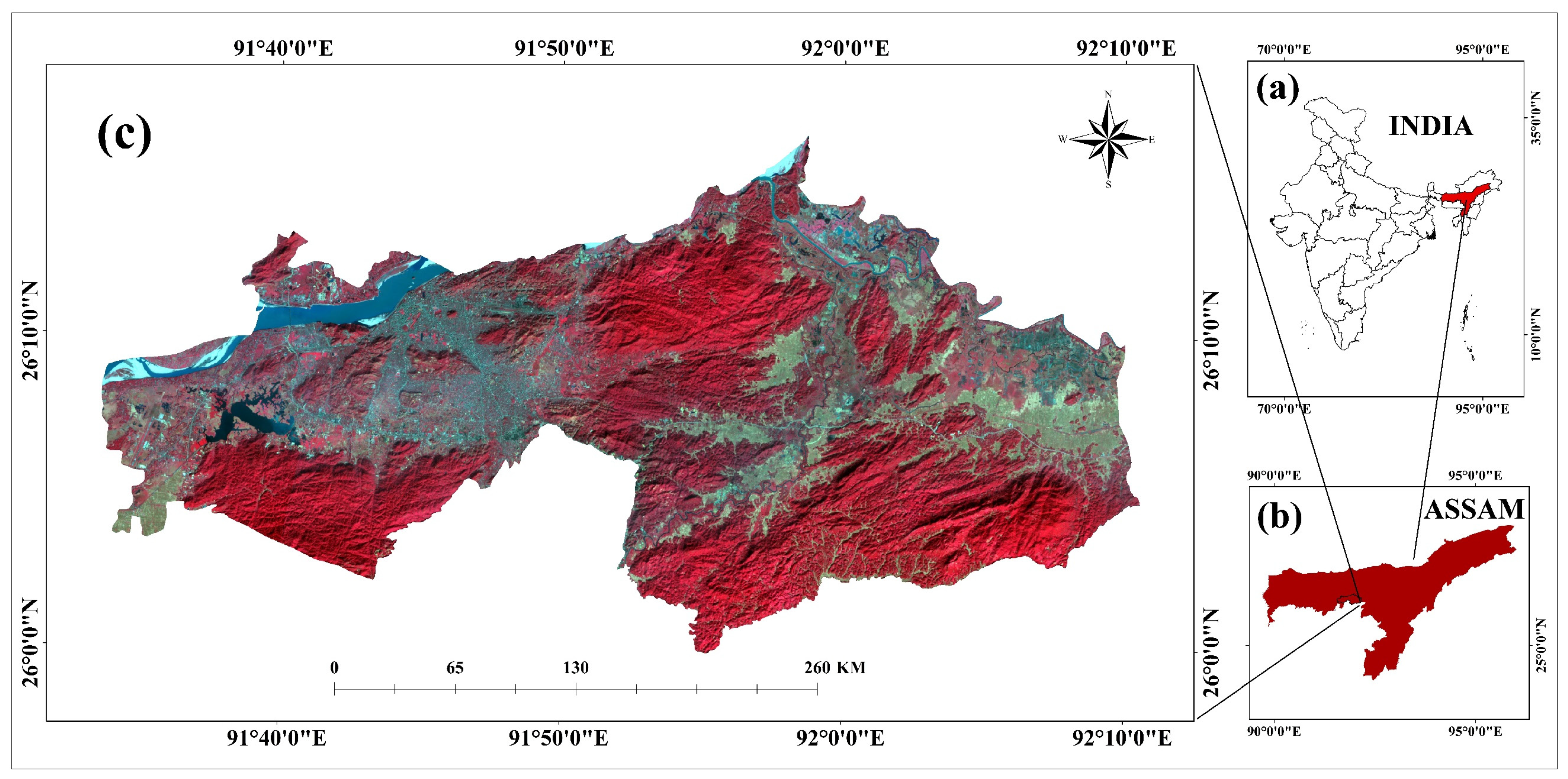
Situated in the northeastern region of India, the state of Assam encompasses the Kamrup Metropolitan District, defined by the geographical coordinates of 26.05° N latitude and 91.60° E longitude (Figure 1). Spanning a substantial expanse in the southwest of Assam, the district is characterized by its diverse topography, comprising plains, mountains, and river valleys. The district shares its boundaries with other Assam districts, such as Kamrup Rural, Nalbari, and Darrang.
Recent years have witnessed accelerated urbanization within Kamrup Metropolitan, evidenced by an 18.34% increase in its urban population since the 2001 Census, according to the Census of India (2011). This rapid urban expansion has driven an increase in urban communities, growth in built-up areas, and a surge in population density, now averaging 2010 individuals per square kilometer. Such urbanization can be attributed to rural–urban migration, economic opportunities, and infrastructure development, all of which underline the district’s significant urban transformation.
A significant part of the Kamrup Metropolitan district corresponds to the jurisdiction of the Guwahati Metropolitan Development Authority, with the city of Guwahati acting as the district’s administrative center. As a major urban hub and the capital of Assam, Guwahati’s geographical coordinates span from 91°33′ E to 91°52′ E longitude and 26°2′ N to 26°16′ N latitude. The study area encompasses the Guwahati Municipal Corporation (GMC) zone, which covers 176.2 km2. Here, escalating urbanization has prompted an expansion of built-up areas, often at the cost of plant cover and water bodies, such as wetlands [27].
Despite their importance in moderating surface temperatures, these ecological attributes have considerably declined due to urbanization. Guwahati’s distinct physical features, including mountains, rivers, lakes, and wetlands, contribute to the regional variances in its prevailing mild, humid subtropical climate. The region experiences significant annual rainfall averaging 1082 mm, predominantly during the southwest monsoon period from May to September.
Given the study’s context, the city’s demographics are of prime importance. Guwahati has experienced the most rapid urbanization compared to other northeastern Indian municipalities. The city is nestled between the southern bank of the Brahmaputra River and the lower reaches of the Shillong Plateau. Since becoming the capital of Assam in 1972, Guwahati’s population growth has surged. The GMC’s population has exponentially grown from 43,615 in 1951 to 962,334 in 2011, as per the Census of India 2011. This sharp population increase has led to substantial unplanned urbanization, impacting land use and land cover (LULC) patterns, local climate, and urban health [28,29].

3. Materials and Methods

As presented in Table 1, this study utilized Landsat imagery possessing a moderate resolution of 30 m. Both land use and land cover (LULC) mapping, as well as land surface temperature (LST) layers, were derived from these satellite images. Furthermore, high-resolution imagery from Google Earth was incorporated to evaluate the accuracy of the LULC classification.

3.1. LULC Classification

In the region of interest, five land use and land cover classes were identified: built-up areas, agricultural land, uncultivated land, vegetation, and water bodies. To conduct various modeling tasks, such as image processing, producing categorized land cover and land use maps, and executing spatial analysis, we used ARC Geographic Information Systems (GIS) package, version 10. We classified Landsat 5 and 8 satellite imagery using the supervised method of maximum likelihood classification. To resample the classified images, we maintained a consistent spatial resolution of 30 m × 30 m [30,31]. This specific pixel size was selected to preserve spatial features in the images and ensure no information was lost. Thematic raster maps for each variable were created and analyzed using the Arc Info GIS program, utilizing cells sized 30 m × 30 m. In this supervised classification, each image pixel was assigned to the category most similar to its spectral signature, which corresponded to recognized land cover types, such as urban and forest. We chose several training sites for each class to represent it, based on consistency with Landsat images, Google Earth, and Google Maps.

3.2. LST Retrieval

The split-window algorithm was employed for extracting the land surface temperature and was chosen for its high accuracy [32]. Thermal infrared bands used by Landsat 8 to image the Earth’s surface were used for LST computation. These bands measure the thermal radiation emitted by the Earth’s surface. However, atmospheric constituents, such as water vapor and aerosols, influence Landsat 8′s thermal bands. Therefore, an atmospheric correction is performed to remove these effects from the LST calculation. This correction utilizes supplementary meteorological data, such as relative humidity and temperature profiles, to model and exclude atmospheric input from the thermal bands [33,34].
Top-of-atmosphere (TOA) reflectance calculation: For LST estimation, understanding surface reflectance across various spectral bands is essential. TOA reflectance is calculated using data from Landsat 8 in both the visible and near-IR bands. The raw digital data from the visible and near-infrared bands are converted into TOA reflectance values using atmospheric correction techniques, which use the Landsat surface reflectance code (LaSRC). The conversion uses the following equation:
Lλ = (ML × Qcal) + AL
where L is the spectral radiation (W/m2/sr/m). ML is the multiplicative rescaling factor for a given band. Quantized and calibrated standard product pixel values are known as Qcal. AL is the additive rescaling factor for a certain band. The information of the Landsat 8 satellite image includes the ML and AL values.
Radiance to brightness temperature conversion: Landsat 8′s thermal bands provide radiance measurements that must be converted into brightness temperature. This conversion takes into account the sensor-specific calibration factors and the radiative transfer equation. The conversion is performed using the following equation:
Tb = K2/ln(1 + (K1/L))
where Tb = brightness temperature in Kelvin; K1, K2 = calibration constants specific to the thermal band; L = measured radiance value. The calibration constants (K1 and K2) can be obtained from the metadata associated with the Landsat 8 image.
NDVI calculation: The NDVI method employs the relationship between vegetation cover and surface emissivity. Areas with high vegetation cover are assumed to have low emissivity, whereas regions with little vegetation cover, such as urban or bare earth areas, have high emissivity. NDVI is calculated using Landsat 8 OLI’s red and near-infrared bands. The NDVI formula is as follows:
NDVI = (NIR − Red)/(NIR + Red)
NIR denotes the spectrum’s reflectance in the near-IR spectrum (spectrum 5). The colour red denotes the spectral reflectance in the red band (Band 4).
Calculation of proportion of vegetation (Pv): The calculation of vegetation proportion (Pv) is critical in LST estimations, particularly in the split-window method. Pv accounts for the cooling effect of vegetation and increases LST retrieval accuracy by considering the fractional coverage of greenery within a pixel or region. Pv is calculated as follows:
Pv = Square ((NDVI − NDVImin)/(NDVImax − NDVImin))
Squaring the normalized difference term improves the distinction amongst vegetation and non-vegetation zones. Through squaring the value, the existence of vegetation is highlighted, making the reaction more sensitive to fluctuations in plant cover.
Surface emissivity: Emissivity is crucial in estimating land surface temperature (LST), as it helps convert recorded thermal radiation into temperature readings. It is represented by the following equation:
ε = 0.004 * Pv + 0.986
where Pv denotes the ratio of vegetation on the ground surface. The constant value 0.004 is employed for scaling the influence of vegetation to total emissivity. The degree of emissivity of non-vegetated backdrops is represented by the constant number 0.986.
LST calculation: LST estimation is a procedure that uses remote sensing data from the Landsat 8 satellite to compute the average temperature of the Earth’s outermost layer. The estimation uses the following formula:
LST = (BT/(1 + (0.00115 * BT/1.4388) * Ln(ε)))
This is a simplified version of the Planck’s law-based technique for estimating land surface temperature (LST) using brightness temperature (BT) and emissivity (ε). BT denotes the computed brightness temperature in the thermal infrared bands. Ln(ε) indicates the natural logarithmic of the land surface’s emissivity (ε). The constant employed in the equation is the coefficient 0.00115. It is the conversion factor used to scale the BT value. The constant 1.4388 indicates the link between wavelengths and temperature and originates from Planck’s law.

3.3. Correlation Analysis

The Pearson correlation coefficient (r) is a statistical measure used to quantify the strength and direction of the linear correlation between two continuous variables. It evaluates how closely the data points for the two variables cluster around a straight line. Pearson correlation coefficients range between −1 and +1. The Pearson correlation coefficient is calculated using the following formula:
r = (Σ((X_i − X_mean) × (Y_i − Y_mean)))/(n × X_std × Y_std),
where Σ is the summation operator. Individual data points for the two variables are represented by X_i and Y_i. The mean value (averages) of the two variables X and Y are represented by X_mean and Y_mean, respectively. The standard deviations of the two variables X and Y are represented by X_std and Y_std, respectively. The total quantity of data points is represented by n.

3.4. Calculation of Indices

The land use/land cover (LULC) indices, including the NDBI (normalized difference built-up index) and NDVI (normalized difference vegetation index), are calculated using remote sensing data from the red, near-infrared (NIR), and short-wave infrared (SWIR) bands. These indices, frequently used to examine land cover properties, whereas the calculation of NDVI is shown above, the NDBI is calculated using the following formula: [35,36].
NDBI = (SWIR − NIR)/(SWIR + NIR)

3.5. Urban Heat Island Index

Assessing the overall UHI effect across a region using land surface temperature (LST) data over an extended period is challenging, as the severity of the urban heat island (UHI) anomaly can significantly vary over time within a particular location. To address this issue, the UHI index was proposed as a technique for making more accurate predictions [37]. It can be calculated using the following equation:
UHI index = LSTi − LSTmin/LSTmax − LSTmin
where LSTi denotes the spatial spread of land surface temperature (LST) given a certain picture in this equation, whereas LSTmax and LSTmin reflect the maximum and lowest LST values inside that image. The UHI index is used to normalize LST values ranging from 0 to 1. A higher index value corresponds to a greater LST. The index value for built-up regions and bare soil, in particular, surpasses 0.6. Vegetation has an index value of 0.3 to 0.6, whereas water bodies have an index value of 0.3 or below. In a nutshell, the UHI index allows for the comparison and categorization of LST figures, enabling the identification of distinct thermal features across various kinds of land cover, such as built-up regions, plants, and water bodies.

3.6. CA-ANN Modelling

The prediction of LST for the year 2032 was made using the QGIS MOLUSCE plugin module and the cellular automata–artificial neural network (CA-ANN) [38]. This model, adept at documenting the complex relationships and dynamics between land cover parameters, environmental conditions, and human activities, simulates and predicts spatial patterns and changes over time by combining the capabilities of cellular automata and artificial neural networks. The CA-ANN model’s ability to integrate GIS and remote sensing data offers significant insights into understanding and predicting the temporal and spatial trends of land cover transitions [39,40].

4. Results

4.1. LULC Change Analysis

We employed a supervised machine learning algorithm for the extraction of four distinct land use and land cover (LULC) classes spanning the years 2000, 2014, and 2022 [41]. To ascertain the accuracy of the LULC maps’ classification, we randomly selected 100 data points for each year (as depicted in Table 2). The LULC maps’ classification proved to be highly accurate, with an overall accuracy exceeding 85% across all three years [42]. Additionally, the Kappa coefficient, which assesses the concordance between the classified maps and reference data, yielded values surpassing 0.88 throughout the study period (refer to Table 2). This attests to the reliability and consistency of the LULC classification for the time frame under analysis [43].
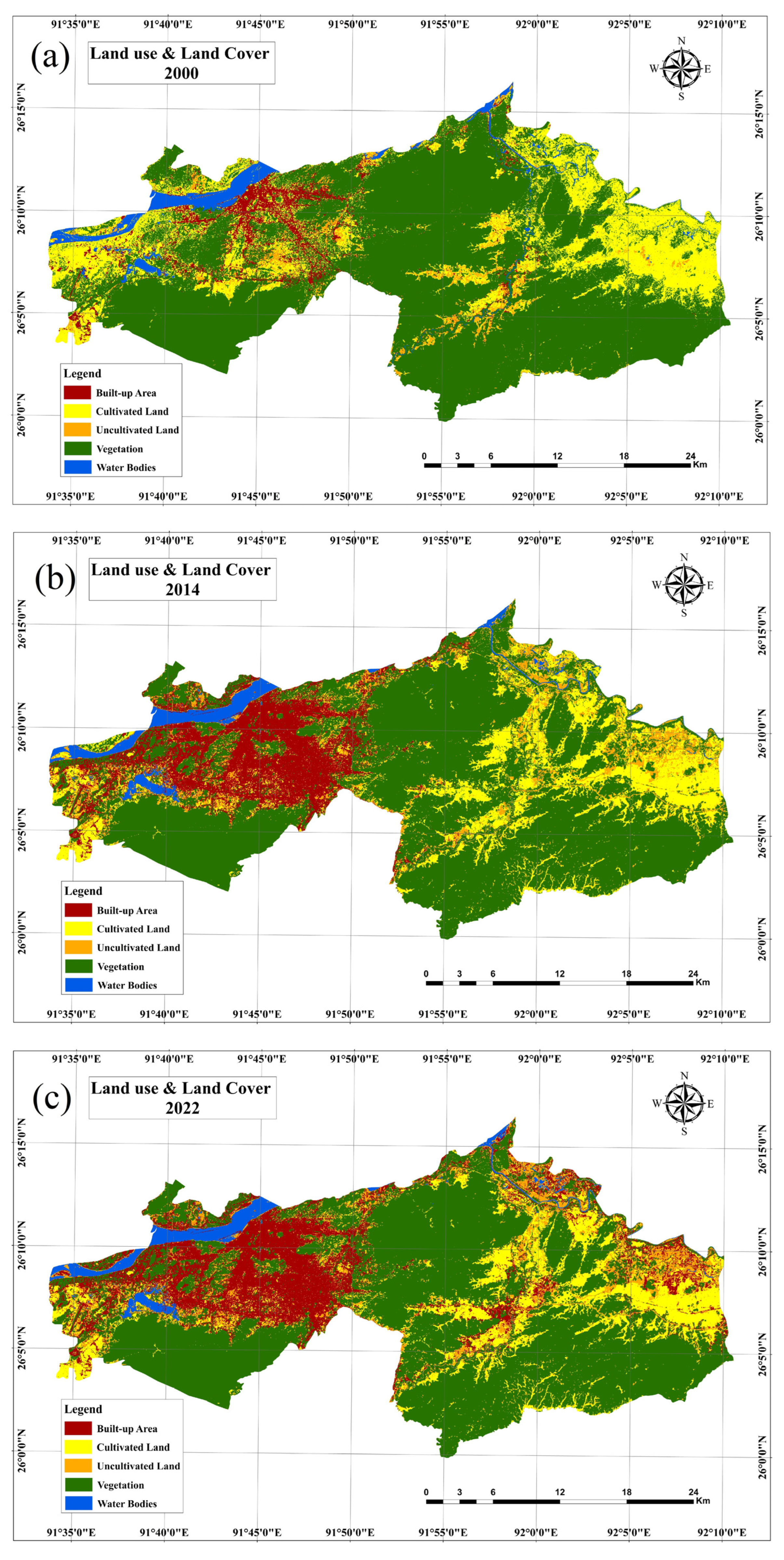
In 2000, cultivated land was the most extensive land cover class, spanning 208.11 square kilometers. However, its area significantly diminished to 134 square kilometers in 2014 and further dwindled to 121.01 square kilometers in 2022. Conversely, the area of uncultivated land increased over this period, growing from 31.58 square kilometers in 2000 to 95 square kilometers in 2014, albeit slightly declining to 94.89 square kilometers in 2022 (Table 3).
Vegetation, encompassing forests, grasslands, and other natural vegetation types, initially covered an expansive 668.99 square kilometers in 2000. This coverage, however, declined to 600 square kilometers in 2014 and further contracted to 459.92 square kilometers by 2022. Additionally, built-up areas, which accounted for 48.63 square kilometers in 2000, witnessed significant growth to 130 square kilometers in 2014 and 166.43 square kilometers in 2022.
The extent of water bodies, comprising lakes, rivers, and reservoirs, was 33.36 square kilometers in 2000, and it remained relatively stable, with a slight decrease to 32 square kilometers in 2014 and 31.67 square kilometers in 2022.
Two key trends emerged from 2000 to 2022. Firstly, the built-up area experienced significant expansion, while the vegetation cover and water bodies underwent contraction. The built-up area surged by a noteworthy percentage over this period, with an average annual growth rate of 9.81 square kilometers per year. Conversely, vegetation cover and water bodies decreased by negative percentages (−35.25% and −5.06%, respectively) from 2000 to 2022, with an average annual decline rate of −17.42 and −0.14 square kilometers per year, respectively. These dynamic trends underscore the evolving nature of the land surface, characterized by the proliferation of built-up areas at the cost of natural land covers and water bodies (as illustrated in Figure 2). The implications of these changes warrant further investigation to assess their potential impact on the ecosystem and local communities [44,45,46].

4.2. Land Surface Temperature (LST) Analysis

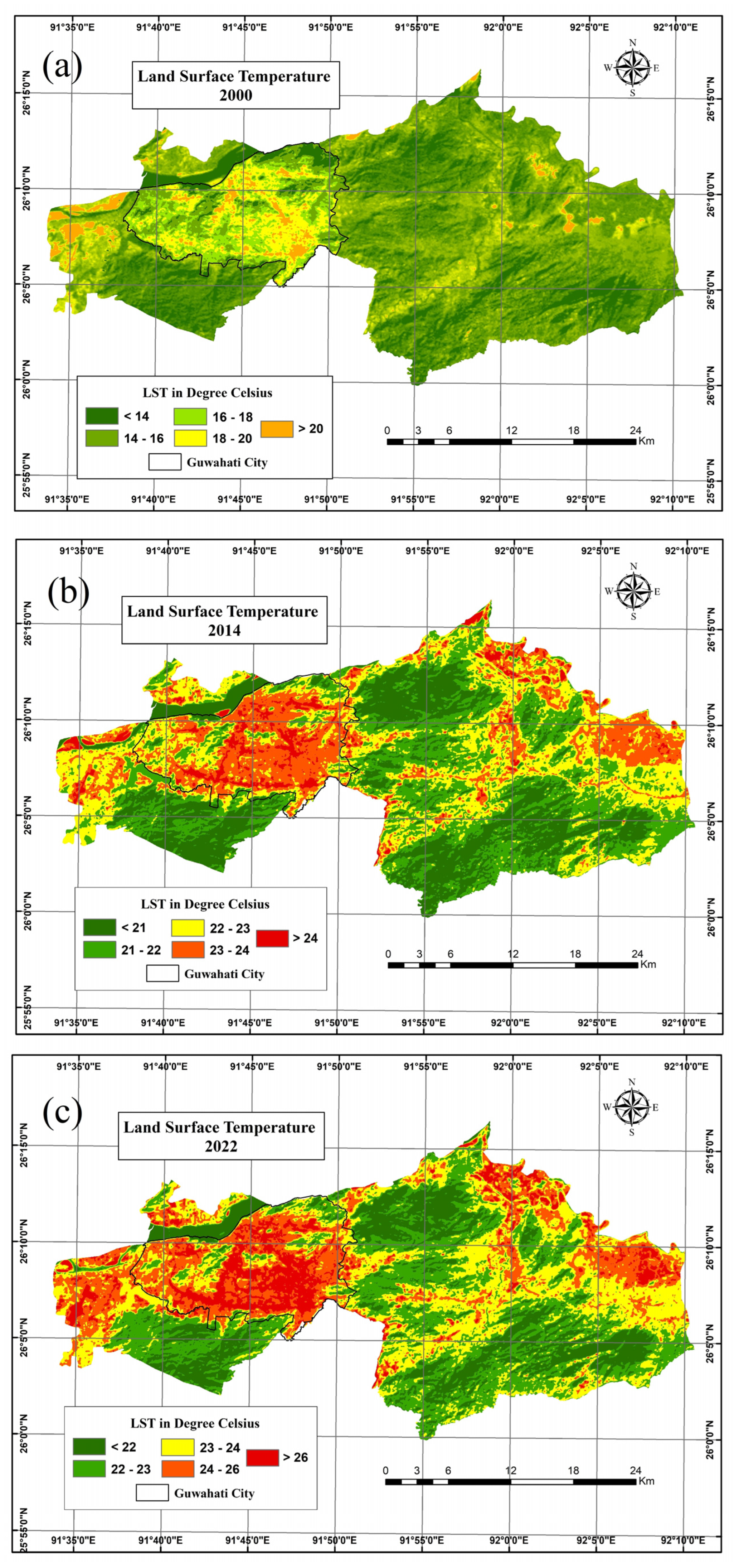
The spatiotemporal distribution of land surface temperature (LST) was evaluated utilizing a combination of equations and Landsat thermal bands throughout the study duration. Figure 3 provides a visual interpretation of the annual LST distribution from 2000 to 2022, demonstrating an escalating trend. The maximum temperature recorded in 2000 was 23.65 °C, significantly increasing to 67.45 °C in 2022, with an annual average shift of 1.990 °C. Correspondingly, the minimum temperature registered in 2000 was 11.85 °C, exhibiting a remarkable rise to 59.26 °C in 2022, with an annual average shift of 2.166 °C. These observations underscore the increasing trend in temperatures during the study period, implicating the potential influence of various factors on LST dynamics [47].
In 2022, the mean LST was noted as 23.652 °C, representing the average land surface temperature. The year’s peak temperature was recorded at 31.322 °C, whereas the lowest temperature was at 18.569 °C. When compared to 2014, a minor decrease in the mean LST was observed. The mean LST in 2014 was 22.606 °C, signifying a slightly higher average temperature than in 2000. The highest and lowest temperatures in 2014 were 29.897 °C and 16.373 °C, respectively. In comparison to the year 2000, there was a substantial increment in the mean LST. The mean LST in 2000 was 16.249 °C, significantly lower than the subsequent years. The maximum and minimum temperatures in 2000 were recorded as 23.657 °C and 11.856 °C, respectively. Overall, these statistics depict a persistent rise in LST from 2000 to 2022, punctuated by a significant increase in mean temperatures. The maximum temperatures also portray an escalating trend, suggesting possible alterations in temperature patterns [47].

4.3. Validation

To verify the accuracy of the prediction results, we initially utilized the cellular automata–artificial neural network (CA-ANN) model to predict land use/land cover (LULC) and land surface temperature (LST) for the 2020s. We subsequently compared the forecasted and estimated maps using the QGIS-MOLUSCE Plugin and Terrset (v 2020) Software programs, employing diverse kappa settings (Table 4, Table 5, Table 6 and Table 7) [48,49]. The assessment results were generally favorable, considering all kappa parameters, accuracy percentages, and overall kappa values surpassing 0.75 and 0.80, respectively. Moreover, the mean error value across all parameters was approximately 20%, further corroborating the reliability of our findings. Additionally, a cross-tabulation was conducted to enhance our understanding of the validation results, which is elaborated upon in Section 4.4.

4.4. Cross-Tabulation

Using SIMULATED_IMAGE_2022_ (columns) vs. REFERENCE_IMAGE_2022_ (rows), we performed a cross-tabulation.

4.5. Forecasted Land Surface Temperature (LST)

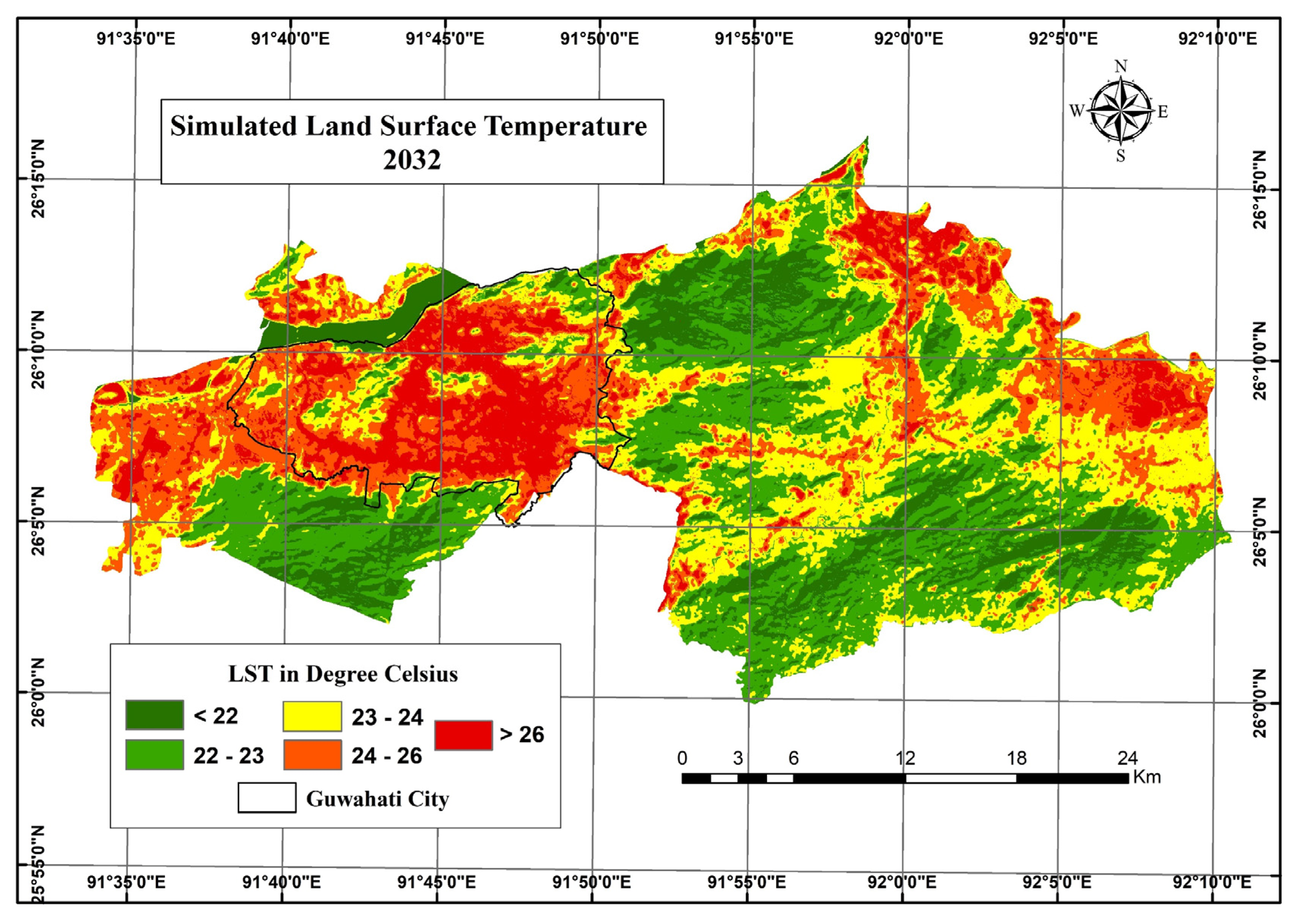
A predictive model was developed based on the prior land surface temperature (LST) dataset to forecast potential LST conditions for the year 2032 (Figure 4). As per the model’s predictions, the creation of higher temperature zones is more probable in the northern and northwestern regions, primarily in areas experiencing extensive urban expansion [47]. The model projects maximum and minimum LST values exceeding 26 °C and below 19 °C, respectively (Table 8). This simulation aligns with the observed increase in LST from 2000 to 2022, largely attributed to the expansion of built-up areas, thereby considerably affecting LST values.
The intensified urban heat island (UHI) effect and the surge in LST are directly linked to the broadening urban footprints and depletion of vegetative cover [47]. The contributing factors for escalating temperatures and UHI impact are multifold, and include urbanization, alterations to the greenhouse gas effect, global warming, and modifications in surface features [50,51,52]. The projected LST scenarios underline the grave concerns associated with this rising trend, such as the heightened UHI effect.

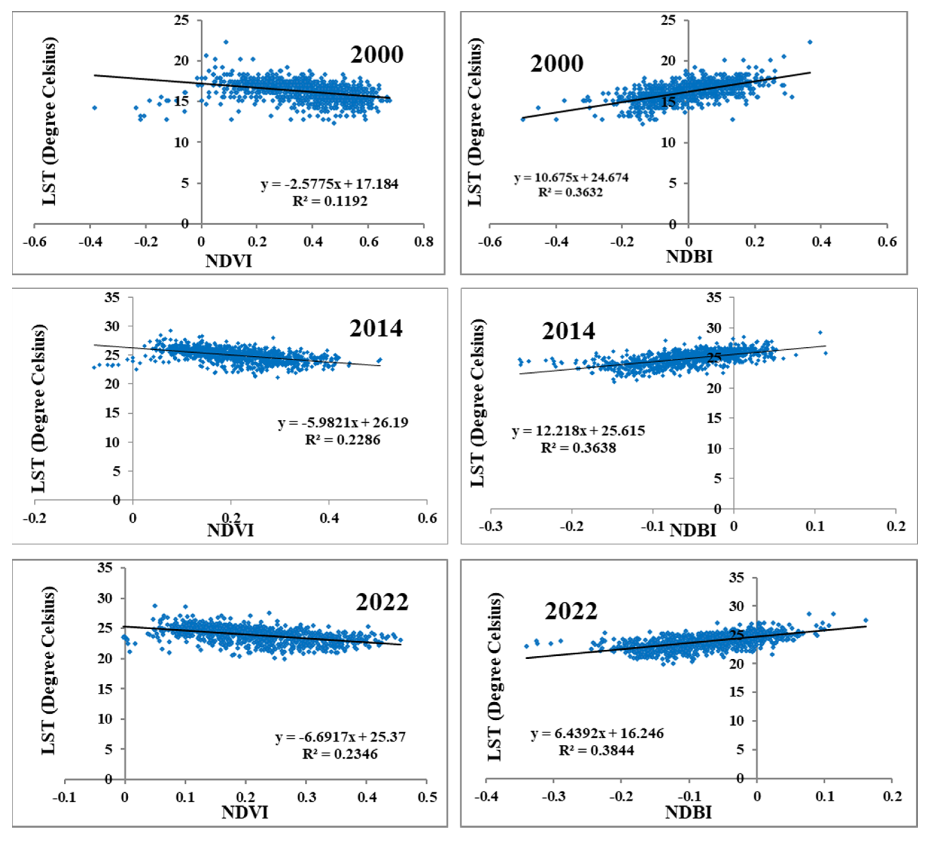
4.6. Interplay between Land Use/Land Cover (LULC) Indices

The presented correlation coefficients (R2) (refer to Figure 5) that detail the relationship between the normalized difference built-up index (NDBI) and land surface temperature (LST) for the years 2000, 2014, and 2022 exhibit compelling patterns. There is a subtle uptick in the correlation coefficient from 2000 to 2022, denoting an intensifying relationship. The linear regression models for each year suggest a consistent positive relationship between LST and NDBI, albeit with variable slopes and intercepts.
In 2000, the positive slope of 10.675x signals a strong influence of LST on NDBI, with an intercept of 24.674. The R2 value of 0.3632 implies that approximately 36.32% of the NDBI variability can be accounted for by LST during this year. Similarly, in 2014 and 2022, the models project positive slopes of 12.218x and 6.4392x, respectively, indicating an ongoing positive relationship between LST and NDBI, albeit with divergent magnitudes. The intercepts for 2014 and 2022 stand at 25.615 and 16.246, respectively. The respective R2 values of 0.3638 and 0.3844 imply that roughly 36.38% and 38.44% of the NDBI variability can be ascribed to LST during these years. This suggests that the influence of built-up areas on temperature patterns has become more significant, with NDBI serving as a more potent predictor of LST variations.
Conversely, an analysis of the relationship between LST and the normalized difference vegetation index (NDVI) for the Kamrup Metro Region across 2000, 2014, and 2022 reveals a different dynamic. The models demonstrate a negative relationship between LST and NDVI, with fluctuating slopes and intercepts. In 2000, the equation projects a steeper negative slope of −5.9821x, suggesting a considerable impact of LST on NDVI, with an intercept of 26.19. Nevertheless, the R2 value of 0.1192 indicates that only around 11.92% of the NDVI variability can be accounted for by LST during this year.
In 2014 and 2022, the models present negative slopes of −6.6917x and −2.5775x, respectively, signifying a weakening relationship between LST and NDVI. The intercepts for 2014 and 2022 stand at 25.37 and 17.184, respectively. The respective R2 values of 0.2286 and 0.2346 suggest that around 22.86% and 23.46% of the NDVI variability can be ascribed to LST during these years. These findings indicate that although vegetation coverage (measured by NDVI) might influence temperature patterns, other factors, such as urbanization, surface characteristics, and localized climatic conditions, likely play a more decisive role in governing LST fluctuations [53,54].

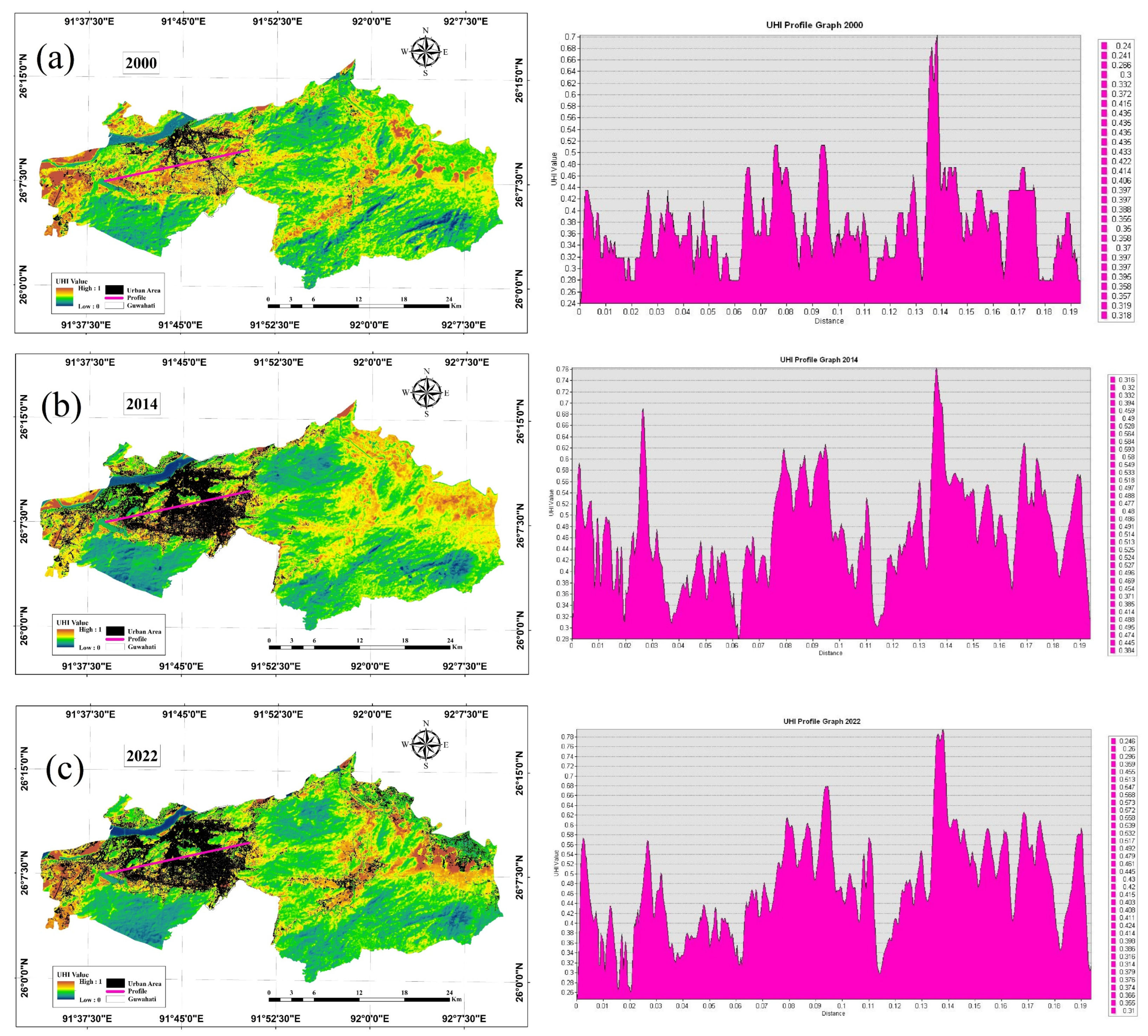
4.7. Urban Heat Island Profile

The urban heat island (UHI) profile, as depicted in Figure 6, is based on a west–east transect drawn across the city of Guwahati, an area characterized by high concentrations of built-up regions. The temperature distribution along this line demonstrates that urban centers typically exhibit higher temperatures compared to their surrounding suburban counterparts. However, a detailed examination reveals a series of temperature peaks and valleys, highlighting distinct thermal variations across the city.
These fluctuations are directly linked to the city’s unique geographic features. The valleys, which correspond to areas with relatively cooler temperatures, are often associated with farmlands, bodies of water, and parks enriched with green spaces. Nearby vegetation-covered areas also play a pivotal role in creating these cooler zones.
In 2000, the highest UHI values appear at a distance of 0.7 on the transect, interspersed with several valleys or dips in the graph at distances of 0.02, 0.06, and 0.18. These dips record UHI values of less than 0.3, implying the presence of significant vegetation cover.
As we progress from 2000 to 2014, there is a noticeable increase in temperatures. The peak at a distance of 0.14 escalates to a UHI value of 0.76, while the valleys at distances of 0.02, 0.06, and 0.18 simultaneously rise to values of 0.31, 0.34, and 0.38, respectively. This uptrend continues into 2022, with the UHI value at a distance of 0.14 surging to 0.78.
The 2014 and 2022 profiles portray an increasing formation of heat islands. This trend is marked by a growth in the number of temperature peaks (high temperatures) and a decrease in the number of valleys (low temperatures), indicating an escalating UHI effect as urban areas expand and vegetation cover reduces. This development is corroborated by the land use/land cover (LULC) analysis conducted from 2000 to 2022.

5. Discussion

The projected future scenario of the Kamrup Metro Region can be extrapolated from the various factors explored in this study. The land use/land cover (LULC) changes revealed a notable transformation in the land surface composition over time, characterized by an expansion of built-up areas at the expense of natural land cover and water bodies [55,56,57,58]. This trend not only demonstrates an ongoing process of urbanization but also suggests its likely continuation in the future.
The land surface temperature (LST) analysis further underscored a persistent and significant uptick in land surface temperatures, especially a remarkable rise in mean temperatures from 2000 to 2022. This escalation in temperature is intrinsically tied to the proliferation of built-up areas, thus, spotlighting the urban heat island (UHI) effect [59]. Predicted LST scenarios for 2032 suggest the emergence of hotter zones, predominantly in the northern and northwestern regions, which are undergoing significant urban development. These predictions signal an impending amplification of the UHI effect, raising serious concerns about its implications for the region’s socio-economic and environmental sustainability.
Moreover, the correlation analysis between the LULC indices exposed a critical insight. While the built-up areas are gaining more influence on temperature patterns, vegetation cover seems to have a diminishing effect on temperature modulation. This trend suggests a systemic imbalance between urbanization and environmental preservation, reinforcing the consequential rise in temperatures and UHI effect [60].
Collectively, these results indicate that the Kamrup Metro Region is on a trajectory towards increased urbanization, heightened temperatures, and amplified UHI effect. The potential impacts of this pathway are vast, encompassing changes in local climate, increased energy consumption, public health risks, and threats to biodiversity, among others [61,62,63].
These findings underscore the urgency of implementing sustainable land management and urban planning strategies [64]. Efforts must focus on preserving and restoring natural land cover to counterbalance the adverse effects of urban sprawl and climate change [65]. Green infrastructure, such as urban green spaces, green roofs, and street trees, could play a crucial role in mitigating the UHI effect. Moreover, sustainable urban planning can promote compact development, reducing the need for land conversion and, thus, preserving natural habitats. Policymakers and urban planners should also prioritize climate resilience in their strategies, considering the vulnerability of urban areas to climate change.
This study serves as a clarion call for a balance between urban growth and environmental preservation, illuminating the critical need for sustainable solutions to manage urban heat islands and mitigate climate change impacts. It underscores the imperative to bridge the divide between economic development and environmental conservation, as the future of the Kamrup Metro Region hangs in the balance.

6. Conclusions

The interplay between land use and land cover (LULC) and land surface temperature (LST) in the Kamrup Metropolitan District region of Northeast India has been deeply examined in this study. The research unfolded through the timescale from 2000 to 2022, offering a well-founded look into the future with projections until 2032. While the conclusions derived are multi-layered and extensive, they are also intricately tied to the limits of the study, opening doors for future research directions. The methodology anchored on a supervised machine learning approach demonstrated that robust and accurate results are achievable. This approach presented reliable mappings of LULC transformations, highlighting an evident shift from cultivated land to built-up areas, painting a picture of growing urbanization. Similarly, the upward trend of LST underscored a warming landscape influenced strongly by urban development and decreasing green cover. The robustness of the CA-ANN model used for future LULC and LST predictions was validated, despite the inherent uncertainties in predictive modeling. However, it is worth acknowledging that the model’s accuracy depends heavily on the quality of input data and how representative it is of future conditions, signaling a potential area for enhancement in future studies. Future projections pointed towards heightened LST, particularly in areas projected for urban growth. This correlation between urban expansion and increasing LST was supported by the relationships between LST, NDBI, and NDVI. The study found that the impact of built-up areas on temperature variations overpowered that of vegetation cover, underscoring the significant role of urbanization in escalating temperatures. The analysis of the urban heat island (UHI) effect extended the discussion further by revealing that urban centers exhibited higher temperatures than their suburban counterparts. The fluctuating peaks and valleys in the temperature profile aligned with the spread of built-up areas and shrinking vegetation, providing evidence of the manifestation and intensification of the UHI effect. While the study provides critical insights into the ongoing urbanization process, increasing temperatures, and growing UHI effects, it also points out several limitations and gaps. The reliance on remote sensing data, although powerful, also carries uncertainties related to data quality and resolution. Furthermore, while the machine learning model provides accurate predictions, it also introduces an inherent degree of uncertainty due to its stochastic nature. These limitations not only indicate the need for caution while interpreting the results but also point towards future research directions. In addition, the study leaves some questions unanswered. While it highlights the importance of vegetation in mitigating UHI effect, the detailed role of different types of vegetation and green infrastructure is left unexplored. Additionally, how urban planning strategies can effectively utilize these natural resources to combat the UHI effect warrants further research. Overall, the study provides a comprehensive understanding of the changing LULC and LST dynamics in the Kamrup Metro Region. It emphasizes the significance of sustainable land management and urban planning strategies in mitigating the adverse effects of urban expansion. At the same time, it throws light on areas needing further exploration, ultimately guiding the region towards a sustainable and climate-resilient future.

Author Contributions

Conceptualization, U.C. and S.K.S.; methodology, U.C.; software, U.C.; validation, S.K. and A.K.; formal analysis, S.K.S. and G.M.; investigation, P.K. and U.C; resources, S.K.; data curation, G.M.; writing—original draft preparation, U.C., and G.M.; writing—review and editing, A.K., S.K. and G.M; visualization, G.M.; supervision, S.K.S. and G.M. All authors have read and agreed to the published version of the manuscript.

Funding

This study received no external funding.

Data Availability Statement

The is available on reasonable request from the first author.

Acknowledgments

The authors would like to thank two anonymous reviewers for their valuable feedback and insights that greatly contributed to the improvement of this manuscript.

Conflicts of Interest

The authors declare no conflict of interest.

References

  1. Cook, J.; Nuccitelli, D.; A Green, S.; Richardson, M.; Winkler, B.; Painting, R.; Way, R.; Jacobs, P.; Skuce, A. Quantifying the Consensus on Anthropogenic Global Warming in the Scientific Literature. Environ. Res. Lett. 2013, 8, 024024. [Google Scholar] [CrossRef] [Green Version]
  2. Pall, P.; Aina, T.; Stone, D.A.; Stott, P.A.; Nozawa, T.; Hilberts, A.G.J.; Lohmann, D.; Allen, M.R. Anthropogenic Greenhouse Gas Contribution to Flood Risk in England and Wales in Autumn 2000. Nature 2011, 470, 382–385. [Google Scholar] [CrossRef] [PubMed]
  3. Solomon, S.; Qin, D.; Manning, M.; Chen, Z.; Marquis, M.; Averyt, K.B.; Tignor, M.; Miller, H.L. Climate Change 2007: The Physical Science Basis. Contribution of Working Group I to the Fourth Assessment Report of the Intergovernmental Panel on Climate Change; Cambridge University Press: Cambridge, UK, 2007. [Google Scholar]
  4. Raimi, M.O.; Odubo, T.V.; Omidiji, A.O. Creating the Healthiest Nation: Climate Change and Environmental Health Impacts in Nigeria: A Narrative Review. Sustain. Environ. 2020, 6, 61. [Google Scholar] [CrossRef]
  5. Singh, P.; Kikon, N.; Verma, P. Impact of Land Use Change and Urbanization on Urban Heat Island in Lucknow City, Central India. A Remote Sensing Based Estimate. Sustain. Cities Soc. 2017, 32, 100–114. [Google Scholar] [CrossRef]
  6. Abdulla, K.; Dey, N.N.; Al Rakib, A.; Rahaman, Z.A.; Nasher, N.M.; Bhatt, A. Modeling the Relationship between Land Use/Land Cover and Land Surface Temperature in Dhaka, Bangladesh Using Ca-Ann Algorithm. Environ. Chall. 2021, 4, 100190. [Google Scholar] [CrossRef]
  7. Elvidge, C.D.; Kalita, H.; Choudhury, U.; Rehman, S.; Tripathy, B.R.; Kumar, P. Inter-Calibration and Urban Light Index of DMSP-OLS Night-Time Data for Evaluating the Urbanization Process in Australian Capital Territory; Springer: Berlin/Heidelberg, Germany, 1970. [Google Scholar]
  8. Seto, K.C.; Güneralp, B.; Hutyra, L.R. Global Forecasts of Urban Expansion to 2030 and Direct Impacts on Biodiversity and Carbon Pools. Proc. Natl. Acad. Sci. USA 2012, 109, 16083–16088. [Google Scholar] [CrossRef] [PubMed]
  9. Jallu, S.B.; Shaik, R.U.; Srivastav, R.; Pignatta, G. Assessing the Effect of Covid-19 Lockdown on Surface Urban Heat Island for Different Land Use /Cover Types Using Remote Sensing. Energy Nexus 2022, 5, 100056. [Google Scholar] [CrossRef]
  10. Oke, T.R. The Energetic Basis of the Urban Heat Island. Q. J. R. Meteorol. Soc. 1982, 108, 1–24. [Google Scholar] [CrossRef]
  11. Lo, C.; Quattrochi, D.A. Land-Use and Land-Cover Change, Urban Heat Island Phenomenon, and Health Implications. Photogramm. Eng. Remote Sens. 2003, 69, 1053–1063. [Google Scholar] [CrossRef]
  12. Wellmann, T.; Lausch, A.; Andersson, E.; Knapp, S.; Cortinovis, C.; Jache, J.; Scheuer, S.; Kremer, P.; Mascarenhas, A.; Kraemer, R.; et al. Remote Sensing in Urban Planning: Contributions towards Ecologically Sound Policies? Landsc. Urban Plan. 2020, 204, 103921. [Google Scholar] [CrossRef]
  13. Wang, S.W.; Gebru, B.M.; Lamchin, M.; Kayastha, R.B.; Lee, W.-K. Land Use and Land Cover Change Detection and Prediction in the Kathmandu District of Nepal Using Remote Sensing and GIS. Sustainability 2020, 12, 3925. [Google Scholar] [CrossRef]
  14. Arshad, S.; Ahmad, S.R.; Abbas, S.; Asharf, A.; Siddiqui, N.A.; Islam, Z.U. Quantifying the Contribution of Diminishing Green Spaces and Urban Sprawl to Urban Heat Island Effect in a Rapidly Urbanizing Metropolitan City of Pakistan. Land Use Policy 2022, 113, 105874. [Google Scholar] [CrossRef]
  15. Ranagalage, M.; Estoque, R.C.; Murayama, Y. An Urban Heat Island Study of the Colombo Metropolitan Area, Sri Lanka, Based on Landsat Data (1997–2017). ISPRS Int. J. Geo-Inf. 2017, 6, 189. [Google Scholar] [CrossRef] [Green Version]
  16. Arnfield, A.J. Two Decades of Urban Climate Research: A Review of Turbulence, Exchanges of Energy and Water, and the Urban Heat Island. Int. J. Climatol. 2003, 23, 1–26. [Google Scholar] [CrossRef]
  17. Soydan, O. Effects of Landscape Composition and Patterns on Land Surface Temperature: Urban Heat Island Case Study for Nigde, Turkey. Urban Clim. 2020, 34, 100688. [Google Scholar] [CrossRef]
  18. Abrar, R.; Sarkar, S.K.; Nishtha, K.T.; Talukdar, S.; Shahfahad; Rahman, A.; Islam, A.R.M.T.; Mosavi, A. Assessing the Spatial Mapping of Heat Vulnerability under Urban Heat Island (UHI) Effect in the Dhaka Metropolitan Area. Sustainability 2022, 14, 4945. [Google Scholar] [CrossRef]
  19. Xiao, R.-B.; Ouyang, Z.-Y.; Zheng, H.; Li, W.-F.; Schienke, E.W.; Wang, X.-K. Spatial Pattern of Impervious Surfaces and Their Impacts on Land Surface Temperature in Beijing, China. J. Environ. Sci. 2007, 19, 250–256. [Google Scholar] [CrossRef]
  20. Weng, Q.; Lu, D.; Schubring, J. Estimation of Land Surface Temperature–Vegetation Abundance Relationship for Urban Heat Island Studies. Remote Sens. Environ. 2004, 89, 467–483. [Google Scholar] [CrossRef]
  21. Baeza, S.; Paruelo, J.M. Land Use/Land Cover Change (2000–2014) in the Rio de La Plata Grasslands: An Analysis Based on Modis Ndvi Time Series. Remote Sens. 2020, 12, 381. [Google Scholar] [CrossRef] [Green Version]
  22. Grimm, N.B.; Foster, D.; Groffman, P.; Grove, J.M.; Hopkinson, C.S.; Nadelhoffer, K.J.; Pataki, D.E.; Peters, D.P. The Changing Landscape: Ecosystem Responses to Urbanization and Pollution across Climatic and Societal Gradients. Front. Ecol. Environ. 2008, 6, 264–272. [Google Scholar] [CrossRef] [Green Version]
  23. Edan, M.H.; Maarouf, R.M.; Hasson, J. Predicting the Impacts of Land Use/Land Cover Change on Land Surface Temperature Using Remote Sensing Approach in Al Kut, Iraq. Phys. Chem. Earth Parts A/B/C 2021, 123, 103012. [Google Scholar] [CrossRef]
  24. Fensholt, R.; Sandholt, I.; Stisen, S. Evaluating Modis, Meris, and Vegetation Vegetation Indices Using in Situ Measurements in a Semiarid Environment. IEEE Trans. Geosci. Remote Sens. 2006, 44, 1774–1786. [Google Scholar] [CrossRef]
  25. Feng, Y.; Du, S.; Myint, S.W.; Shu, M. Do Urban Functional Zones Affect Land Surface Temperature Differently? A Case Study of Beijing, China. Remote Sens. 2019, 11, 1802. [Google Scholar] [CrossRef] [Green Version]
  26. McFeeters, S.K. The Use of the Normalized Difference Water Index (NDWI) in the Delineation of Open Water Features. Int. J. Remote Sens. 1996, 17, 1425–1432. [Google Scholar] [CrossRef]
  27. Bhuyan, C. Spatio Temporal Analysis of Urban Expansion and Its Impact on Land Use Land Cover: A Case Study of Guwahati Metropolitan Area. Clar.-Int. Multidiscip. J. 2018, 7, 55. [Google Scholar] [CrossRef]
  28. Talukdar, K.K.; Arsac, A.C. Land Surface Temperature Retrieval of Guwahati City and Suburbs, Assam, India Using Landsat Data. Int. J. Eng. Res. Technol. 2020, 9, 882–887. [Google Scholar] [CrossRef]
  29. Alsharif, A.A.A.; Pradhan, B. Urban Sprawl Analysis of Tripoli Metropolitan City (Libya) Using Remote Sensing Data and Multivariate Logistic Regression Model. J. Indian Soc. Remote Sens. 2013, 42, 149–163. [Google Scholar] [CrossRef]
  30. Liu, Y.-L.; Yan, S.-Y. Study on the Integration of GIS and Remote Sensing Data in Grouping-Interpretation System for Remote Sensing Image. SPIE Proc. 2004, 5573, 452–460. [Google Scholar] [CrossRef]
  31. Rwanga, S.S.; Ndambuki, J.M. Accuracy Assessment of Land Use/Land Cover Classification Using Remote Sensing and GIS. Int. J. Geosci. 2017, 08, 611–622. [Google Scholar] [CrossRef] [Green Version]
  32. Ulivieri, C.; Castronuovo, M.; Francioni, R.; Cardillo, A. A Split Window Algorithm for Estimating Land Surface Temperature from Satellites. Adv. Space Res. 1994, 14, 59–65. [Google Scholar] [CrossRef]
  33. Kumar, B.P.; Babu, K.R.; Anusha, B.; Rajasekhar, M. Geo-Environmental Monitoring and Assessment of Land Degradation and Desertification in the Semi-Arid Regions Using Landsat 8 Oli / TIRS, LST, and NDVI Approach. Environ. Chall. 2022, 8, 100578. [Google Scholar] [CrossRef]
  34. Jacob, B.; Chen, J.; Huang, Y.; Cohen, I. Pearson Correlation Coefficient. In Noise Reduction in Speech Processing; Springer: Berlin/Heidelberg, Germany, 1970. [Google Scholar]
  35. Muhaimin, M.; Fitriani, D.; Adyatma, S.; Arisanty, D. Mapping Build-up Area Density Using Normalized Difference Built-up Index (Ndbi) and Urban Index (UI) Wetland in the City Banjarmasin. IOP Conf. Ser. Earth Environ. Sci. 2022, 1089, 012036. [Google Scholar] [CrossRef]
  36. Huang, S.; Tang, L.; Hupy, J.P.; Wang, Y.; Shao, G.F. A Commentary Review on the Use of Normalized Difference Vegetation Index (NDVI) in the Era of Popular Remote Sensing. J. For. Res. 2020, 32, 1–6. [Google Scholar] [CrossRef]
  37. Aneesh, M.; Khandelwal, S.; Kaul, N. Spatial and Temporal Variations of Urban Heat Island Effect and the Effect of Percentage Impervious Surface Area and Elevation on Land Surface Temperature: Study of Chandigarh City, India. Sustain. Cities Soc. 2016, 26, 264–277. [Google Scholar] [CrossRef]
  38. Ahmad, Y.S.; Sahu, P.; Kalubarme, M.H.; Kansara, B.B. Monitoring Land Use Changes and Its Future Prospects Using Cellular Automata Simulation and Artificial Neural Network for Ahmedabad City, India. GeoJournal 2020, 87, 765–786. [Google Scholar] [CrossRef]
  39. Li, X.; Yeh, A.G.-O. Modelling Sustainable Urban Development by the Integration of Constrained Cellular Automata and GIS. Int. J. Geogr. Inf. Sci. 2000, 14, 131–152. [Google Scholar] [CrossRef]
  40. Bhatta, B.; Saraswati, S.; Bandyopadhyay, D. Urban Sprawl Measurement from Remote Sensing Data. Appl. Geogr. 2010, 30, 731–740. [Google Scholar] [CrossRef]
  41. Lahon, D.; Sahariah, D.; Debnath, J.; Nath, N.; Meraj, G.; Kumar, P.; Hashimoto, S.; Farooq, M. Assessment of Ecosystem Service Value in Response to LULC Changes Using Geospatial Techniques: A Case Study in the Merbil Wetland of the Brahmaputra Valley, Assam, India. ISPRS Int. J. Geo-Inf. 2023, 12, 165. [Google Scholar] [CrossRef]
  42. Singh, S.; Singh, S.K.; Prajapat, D.K.; Pandey, V.; Kanga, S.; Kumar, P.; Meraj, G. Assessing the Impact of the 2004 Indian Ocean Tsunami on South Andaman’s Coastal Shoreline: A Geospatial Analysis of Erosion and Accretion Patterns. J. Mar. Sci. Eng. 2023, 11, 1134. [Google Scholar] [CrossRef]
  43. Debnath, J.; Sahariah, D.; Saikia, A.; Meraj, G.; Nath, N.; Lahon, D.; Annayat, W.; Kumar, P.; Chand, K.; Singh, S.K.; et al. Shifting Sands: Assessing Bankline Shift Using an Automated Approach in the Jia Bharali River, India. Land 2023, 12, 703. [Google Scholar] [CrossRef]
  44. Bera, A.; Meraj, G.; Kanga, S.; Farooq, M.; Singh, S.K.; Sahu, N.; Kumar, P. Vulnerability and Risk Assessment to Climate Change in Sagar Island, India. Water 2022, 14, 823. [Google Scholar] [CrossRef]
  45. Meraj, G. Assessing the Impacts of Climate Change on Ecosystem Service Provisioning in Kashmir Valley India. Ph.D. Thesis, Suresh Gyan Vihar University, Jaipur, India, 2021. Available online: http://hdl.handle.net/10603/354338 (accessed on 15 October 2022).
  46. Meraj, G. Ecosystem service provisioning–underlying principles and techniques. SGVU J. Clim. Chang. Water 2020, 7, 56–64. [Google Scholar]
  47. Kanga, S.; Meraj, G.; Johnson, B.A.; Singh, S.K.; PV, M.N.; Farooq, M.; Kumar, P.; Marazi, A.; Sahu, N. Understanding the Linkage between Urban Growth and Land Surface Temperature—A Case Study of Bangalore City, India. Remote Sens. 2022, 14, 4241. [Google Scholar] [CrossRef]
  48. Nath, N.; Sahariah, D.; Meraj, G.; Debnath, J.; Kumar, P.; Lahon, D.; Chand, K.; Farooq, M.; Chandan, P.; Singh, S.K.; et al. Land Use and Land Cover Change Monitoring and Prediction of a UNESCO World Heritage Site: Kaziranga Eco-Sensitive Zone Using Cellular Automata-Markov Model. Land 2023, 12, 151. [Google Scholar] [CrossRef]
  49. Sajan, B.; Mishra, V.N.; Kanga, S.; Meraj, G.; Singh, S.K.; Kumar, P. Cellular Automata-Based Artificial Neural Network Model for Assessing Past, Present, and Future Land Use/Land Cover Dynamics. Agronomy 2022, 12, 2772. [Google Scholar] [CrossRef]
  50. Tomar, P.; Singh, S.K.; Kanga, S.; Meraj, G.; Kranjčić, N.; Đurin, B.; Pattanaik, A. GIS-Based Urban Flood Risk Assessment and Management—A Case Study of Delhi National Capital Territory (NCT), India. Sustainability 2021, 13, 12850. [Google Scholar] [CrossRef]
  51. Singh, S.; Singh, H.; Sharma, V.; Shrivastava, V.; Kumar, P.; Kanga, S.; Sahu, N.; Meraj, G.; Farooq, M.; Singh, S.K. Impact of Forest Fires on Air Quality in Wolgan Valley, New South Wales, Australia—A Mapping and Monitoring Study Using Google Earth Engine. Forests 2022, 13, 4. [Google Scholar] [CrossRef]
  52. Chand, K.; Kuniyal, J.C.; Kanga, S.; Guleria, R.P.; Meraj, G.; Kumar, P.; Farooq, M.; Singh, S.K.; Nathawat, M.S.; Sahu, N.; et al. Aerosol Characteristics and Their Impact on the Himalayan Energy Budget. Sustainability 2022, 14, 179. [Google Scholar] [CrossRef]
  53. Singh, H.; Meraj, G.; Singh, S.; Shrivastava, V.; Sharma, V.; Farooq, M.; Kanga, S.; Singh, S.K.; Kumar, P. Status of Air Pollution during COVID-19-Induced Lockdown in Delhi, India. Atmosphere 2022, 13, 2090. [Google Scholar] [CrossRef]
  54. Meraj, G.; Kanga, S.; Ambadkar, A.; Kumar, P.; Singh, S.K.; Farooq, M.; Johnson, B.A.; Rai, A.; Sahu, N. Assessing the Yield of Wheat Using Satellite Remote Sensing-Based Machine Learning Algorithms and Simulation Modeling. Remote Sens. 2022, 14, 3005. [Google Scholar] [CrossRef]
  55. Meraj, G.; Khan, T.; Romshoo, S.A.; Farooq, M.; Rohitashw, K.; Sheikh, B.A. An Integrated Geoinformatics and Hydrological Modelling-Based Approach for Effective Flood Management in the Jhelum Basin, NW Himalaya. Proceedings 2019, 7, 8. [Google Scholar] [CrossRef]
  56. Meraj, G.; Kanga, S.; Kranjčić, N.; Đurin, B.; Singh, S.K. Role of Natural Capital Economics for Sustainable Management of Earth Resources. Earth 2021, 2, 622–634. [Google Scholar] [CrossRef]
  57. Kanga, S.; Singh, S.K.; Meraj, G.; Kumar, A.; Parveen, R.; Kranjčić, N.; Đurin, B. Assessment of the Impact of Urbanization on Geoenvironmental Settings Using Geospatial Techniques: A Study of Panchkula District, Haryana. Geographies 2022, 2, 1–10. [Google Scholar] [CrossRef]
  58. Shyam, M.; Meraj, G.; Kanga, S.; Sudhanshu; Farooq, M.; Singh, S.K.; Sahu, N.; Kumar, P. Assessing the Groundwater Reserves of the Udaipur District, Aravalli Range, India, Using Geospatial Techniques. Water 2022, 14, 648. [Google Scholar] [CrossRef]
  59. Dijoo, Z.K. Urban Heat Island Effect Concept and Its Assessment Using Satellite-Based Remote Sensing Data. In Geographic Information Science for Land Resource Management; Wiley: New York, NY, USA, 2021; pp. 81–98. [Google Scholar]
  60. Bashir, O.; Bangroo, S.A.; Guo, W.; Meraj, G.T.; Ayele, G.; Naikoo, N.B.; Shafai, S.; Singh, P.; Muslim, M.; Taddese, H.; et al. Simulating Spatiotemporal Changes in Land Use and Land Cover of the North-Western Himalayan Region Using Markov Chain Analysis. Land 2022, 11, 2276. [Google Scholar] [CrossRef]
  61. Rather, M.A.; Meraj, G.; Farooq, M.; Shiekh, B.A.; Kumar, P.; Kanga, S.; Singh, S.K.; Sahu, N.; Tiwari, S.P. Identifying the Potential Dam Sites to Avert the Risk of Catastrophic Floods in the Jhelum Basin, Kashmir, NW Himalaya, India. Remote Sens. 2022, 14, 1538. [Google Scholar] [CrossRef]
  62. Fayaz, M.; Meraj, G.; Khader, S.A.; Farooq, M.; Kanga, S.; Singh, S.K.; Kumar, P.; Sahu, N. Management of Landslides in a Rural–Urban Transition Zone Using Machine Learning Algorithms—A Case Study of a National Highway (NH-44), India, in the Rugged Himalayan Terrains. Land 2022, 11, 884. [Google Scholar] [CrossRef]
  63. Ahmed, R.; Rawat, M.; Wani, G.F.; Ahmad, S.T.; Ahmed, P.; Jain, S.K.; Meraj, G.; Mir, R.A.; Rather, A.F.; Farooq, M. Glacial Lake Outburst Flood Hazard and Risk Assessment of Gangabal Lake in the Upper Jhelum Basin of Kashmir Himalaya Using Geospatial Technology and Hydrodynamic Modeling. Remote Sens. 2022, 14, 5957. [Google Scholar] [CrossRef]
  64. Meraj, G.; Farooq, M.; Singh, S.K.; Islam, M.; Kanga, S. Modeling the sediment retention and ecosystem provisioning services in the Kashmir valley, India, Western Himalayas. Model. Earth Syst. Environ. 2021, 8, 3859–3884. [Google Scholar] [CrossRef]
  65. Meraj, G.; Singh, S.K.; Kanga, S.; Islam, M. Modeling on comparison of ecosystem services concepts, tools, methods and their ecological-economic implications: A review. Model. Earth Syst. Environ. 2021, 8, 15–34. [Google Scholar] [CrossRef]
Figure 1. False colour composite (FCC) Landsat 8 OLI image representing the location of the study area, Kamrup Metropolitan District. (a) India, (b) the state of Assam, and (c) study area.
Earth 04 00026 g001
Figure 2. Land use and land cover classification for the years (a) 2000, (b) 2014, and (c) 2022.
Earth 04 00026 g002
Figure 3. Land surface temperature estimation for the years (a) 2000, (b) 2014, and (c) 2022.
Earth 04 00026 g003
Figure 4. Simulated land surface temperature (LST) using CA-ANN algorithm for the year 2023.
Earth 04 00026 g004
Figure 5. The above figure represents the correlation analysis between LST with NDVI and NDBI for 2000, 2014, and 2022.
Earth 04 00026 g005
Figure 6. Urban heat island data along with the graphical representation of the profile surface, (a) 2000. (b) 2014, and (c) 2022.
Earth 04 00026 g006
Table 1. Landsat 5 and 8 data (sensors and resolution).
DateSensorsPath/RowResolution
2 November 2000Landsat 5 TM137/4230
9 November 2014Landsat 8 OLI137/4230
15 November 2022Landsat 8 OLI137/4230
Table 2. Accuracy assessment using kappa statistics for LULC (2000, 2014, and 2022).
User’s Accuracy (%)Producer’s Accuracy (%)Overall Accuracy (%)Kappa
YearsBuilt-UpCultivated LandUncultivated LandVegetationWater BodyBuilt-UpCultivated LandUncultivated LandVegetationWater Body
200098.690.98099.46878999.8591.282.390970.942
20149299.3499.269599.4499.299.6794.117099.76960.935
202271.287.599.8999.6799.7899.693.3372.7298.3666.66940.897
Table 3. LULC Change Detection from 2000 to 2022 in Square Kilometer.
Class Name/YearArea in 2000 (sq. km)Area in 2014 (sq. km)Area in 2022 (sq. km)
Cultivated land208.12134121
Uncultivated land31.589594.88
Vegetation668.98600459.92
Built-up48.63130166.42
Water body33.363231.67
Table 4. Validation statistics for the derived LST 2022.
Validation Parameters of QGIS MOLUSCE Plugin Using CA-ANN
Year% of correctnessKappa (Overall)Kappa (Histo)Kappa (loc)
LST 202275.590.850.770.83
Earth 04 00026 i001
Table 5. Pixel Cross-tabulation.
Category012345Total
01,042,55141811241,042,590
1 (<21 °C)0145,02835,115643269490181,545
2 (21–22 °C)0101,867191,00211,956219568305,612
3 (22–23 °C)0390745,318239,02535497156298,955
4 (23–24 °C)0120729543,730154,0288687213,860
5 (>24 °C)00231598112,49182,154100,857
Total1,042,551250,926278,979301,346170,55899,0592,143,419
Chi-square = 6,606,358.5000, degree of freedom (df) = 25, p-Level = 0.0000, Cramer’s V = 0.7851
Table 6. Proportional Cross-tabulation.
Category012345Total
00.48640.00000.00000.00000.00000.00000.4864
1 (<21 °C)0.00000.06770.01640.00030.00010.00020.0847
2 (21–22 °C)0.00000.04750.08910.00560.00010.00030.1426
3 (22–23 °C)0.00000.00180.02110.11150.00170.00330.1395
4 (23–24 °C)0.00000.00010.00340.02040.07190.00410.0998
5 (>24 °C)0.00000.00000.00010.00280.00580.03830.0471
Total0.48640.11710.13020.14060.07960.04621.0000
Table 7. Kappa index of agreement (KIA).
Using Reference Image 2022
as the reference image
CategoryKIA
00.9999
10.7722
20.5689
30.7667
40.696
50.8056
Using Simulated Image_2022
as the reference image
CategoryKIA
00.9999
10.7722
20.5689
30.7667
40.696
50.8056
Overall kappa: 0.8084
Table 8. Values showing the LST (mean, max, min) from 2000 to 2022 along with simulated 2032.
LST2000201420222032
MEAN16.24962.60623.65223.956
MAX23.65729.89731.32232.147
MIN11.85616.37318.56919.623
Disclaimer/Publisher’s Note: The statements, opinions and data contained in all publications are solely those of the individual author(s) and contributor(s) and not of MDPI and/or the editor(s). MDPI and/or the editor(s) disclaim responsibility for any injury to people or property resulting from any ideas, methods, instructions or products referred to in the content.

