Deep Learning Models Outperform Generalized Machine Learning Models in Predicting Winter Wheat Yield Based on Multispectral Data from Drones

Abstract

Timely and accurate monitoring of winter wheat yields is beneficial for the macro-guidance of agricultural production and for making precise management decisions throughout the winter wheat reproductive period. The accuracy of crop yield prediction can be improved by combining unmanned aerial vehicle (UAV)-based multispectral data with deep learning algorithms. In this study, 16 yield-sensitive vegetation indices were constructed, and their correlations were analyzed based on UAV multispectral data of winter wheat at the heading, flowering, and filling stages. Seven input variable sets were obtained based on the combination of data from these three periods, and four generalized machine learning algorithms (Random Forest (RF), K-Nearest Neighbor (KNN), Bagging, and Gradient Boosting Regression (GBR)) and one deep learning algorithm (1D Convolutional Neural Network (1D-CNN)) were used to predict winter wheat yield. The results showed that the RF model had the best prediction performance among the generalised machine learning models. The CNN model achieved the best prediction accuracy based on all seven sets of input variables. Generalised machine learning models tended to underestimate or overestimate yields under different irrigation treatments, with good prediction performance for observed yields < 7.745 t·ha⁻¹. The CNN model showed the best prediction performance based on most input variable groups across the range of observed yields. Most of the differences between observed and predicted values (Y_i) for the CNN models were distributed between −0.1 t·ha⁻¹ and 0.1 t·ha⁻¹, and the model was relatively stable. Therefore, the CNN model is recommended in this study for yield prediction and as a reference for future precision agriculture research.

1. Introduction

Winter wheat is a vital food crop in both northern China and worldwide, where the demand for winter wheat is increasing due to the growing world population and rapid economic development [1]. Therefore, accurate winter wheat yield predictions are crucial to ensuring food security and promoting agricultural production. Winter wheat yield forecasting has long been an important area of research in agriculture. Traditional yield forecasting methods are mainly based on manual surveys and statistics. This involves collecting a range of information, including growth and meteorological data, followed by data analysis and modelling [2]. This approach is not only time-consuming and laborious but also challenging to ensure accuracy. In recent years, the continuous progress of science and technology has opened up new opportunities for winter wheat yield prediction with the application of new technologies such as remote sensing technology, which has great potential in this field.

Compared with traditional methods, remote sensing technology has great potential for winter wheat yield prediction. With the continuous development of modern technology, remote sensing technology is being increasingly used in various fields, such as environmental monitoring [3] and agricultural precision management [4]. Manual methods of remote sensing data collection are not only inefficient but also costly [5]. Satellite remote sensing has advantages such as a wide collection area and good resolution; however, its actual impact is often unsatisfactory due to its long acquisition time and susceptibility to weather, cloud cover, and sensor technology [6]. In contrast, the emerging technology of UAV remote sensing platforms can carry a variety of sensors with high resolution, flexibility, convenience, and low cost. These platforms can overcome the limitations of satellite remote sensing technology and quickly and efficiently obtain data on the growth status [7] and soil moisture [8] of winter wheat at different fertility stages. Artificial intelligence and big data analysis can be used to process and analyse the data [9], resulting in more accurate yield predictions. The UAV remote sensing platform with multispectral sensors has been used to non-destructively assess LAI [10], biomass [11], yield [12], chlorophyll content [13], and N-use efficiency [14] of different materials with good results.

Machine learning algorithms are widely used in agriculture, using mathematical and statistical methods to enable computers to learn from data and improve performance without explicit instruction [15]. For maize yield prediction, the RF algorithm has demonstrated high accuracy, outperforming support vector machines and artificial neural network models [16]. At the tuber formation stage for potatoes, the RF algorithm performed best in predicting above-ground biomass while providing satisfactory accuracy at the tuber expansion stage [17]. The K-Nearest Neighbor algorithm has also shown good predictive performance for cassava yield prediction [18]. In the study of chlorophyll content in winter wheat, the Bagging model demonstrated significant accuracy, although it did not perform the best in prediction performance [19]. In addition, the GBR model has shown the best performance in predicting daily evapotranspiration for irrigation planning, providing new ideas for future agricultural water management allocation [20]. Given the demonstrated success of these machine learning algorithms in previous studies, they are well suited for use in winter wheat yield prediction.

Deep learning models, especially 1D CNN models, have gained popularity in various scientific fields [21]. 1D CNN models have the capability of representational learning, which allows them to perform translation invariant classification through the hierarchical structure of the input information [22]. They can be utilised for lossless maize yield prediction and are well-suited for feature extraction and classification [23]. CNNs can also extract effective feature structures from complex spectral data, providing greater model expressiveness and higher performance than traditional models [24]. These characteristics make CNNs highly promising for improving the precision of winter wheat yield prediction, especially during the heading stage, which is a suitable time for data collection [25]. 1D CNNs have been shown to be a promising approach for the detection of water pH, offering higher prediction accuracy and better modelling convenience compared to traditional algorithms without the need for complex pre-processing of input variables [26]. In soil phosphorus content prediction, 1D-CNN is also expected to significantly improve the ability to predict effective phosphorus in soil [27]. Therefore, the 1D-CNN model was chosen for the winter wheat yield prediction.

Although many studies have been conducted on winter wheat yield, few have investigated the construction of winter wheat yield prediction models by combining data from multiple fertility stages and using different machine learning and deep learning algorithms. Therefore, the main objectives of this study were: (1) to evaluate the feasibility of yield prediction using vegetation index data from three fertility stages; (2) to evaluate the predictive performance of yield prediction models based on combinations of vegetation indices from different fertility stages; and (3) to analyse the stability of different models by examining the distribution of differences between observed and predicted yield values Y_i. The results of this study will demonstrate the reliability of using different fertility vegetation indices as input variables for yield prediction, providing an efficient and economical method for future yield prediction research.

2. Materials and Methods

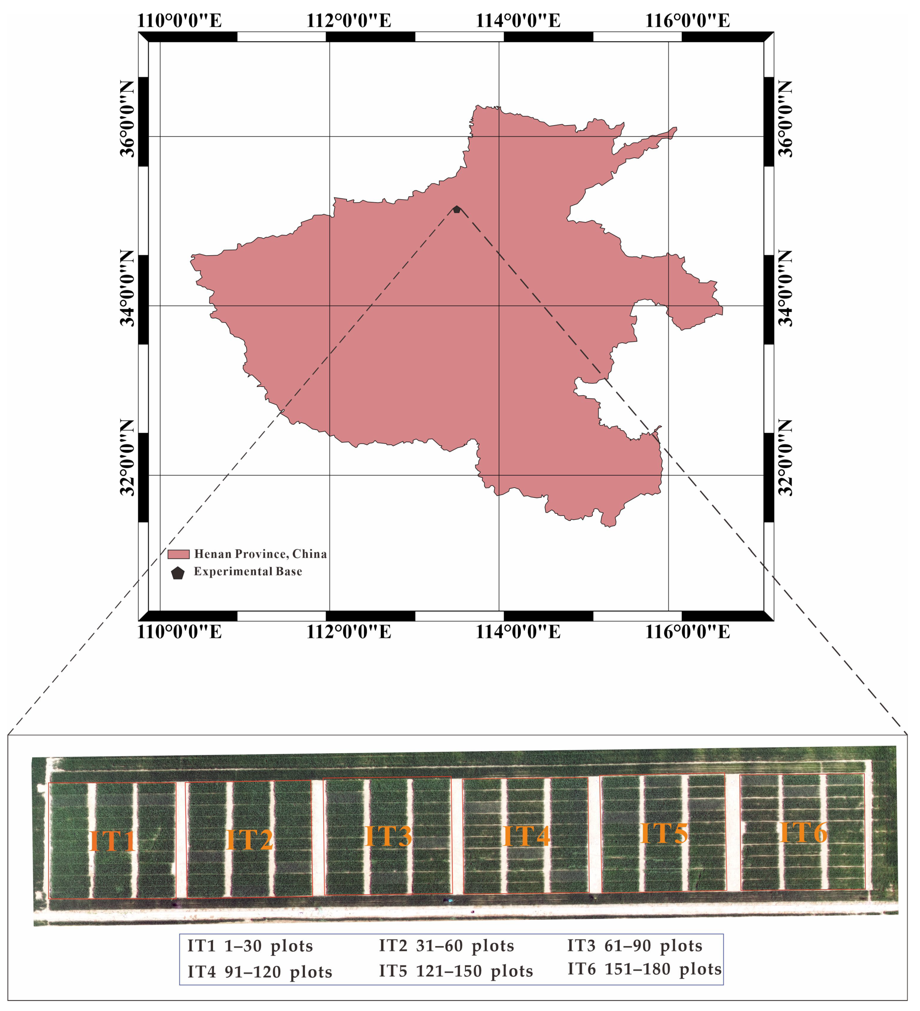
2.1. Experimental Area and Design

This study was conducted at the comprehensive experimental base of the Chinese Academy of Agricultural Sciences in Xinxiang County, Xinxiang City, Henan Province (Figure 1). The study area is located at 113°45′38″ N longitude and 35°8′10″ N latitude, with an altitude of 88 m above sea level and a subtropical monsoon climate characterised by an average annual temperature of 14 °C and an average annual rainfall of 650 mm.

The trial was conducted during the 2021–2022 season and consisted of 180 test plots with six irrigation treatments: IT1 (300 mm, full irrigation water), IT2 (240 mm, 80% full irrigation water), IT3 (180 mm, 60% full irrigation water), IT4 (120 mm, 40% full irrigation water), IT5 (60 mm, 20% full irrigation water), and IT6 (rainfed). These treatments corresponded to plot serial numbers 1–30, 31–60, 61–90, 91–120, 121–150, and 151–180. Ten wheat varieties commonly grown in the North China Plain were planted, with three replications of each variety set up for each treatment. Each treatment consisted of 30 test plots, measuring 4 m long and 1.4 m wide, with adjacent plots spaced 0.4 m apart to the left and right and 1 m apart to the front and back. The trial was sown at the end of October 2021 and harvested by test plot on 5 June 2022, with yield data collected for a total of 180 plots.

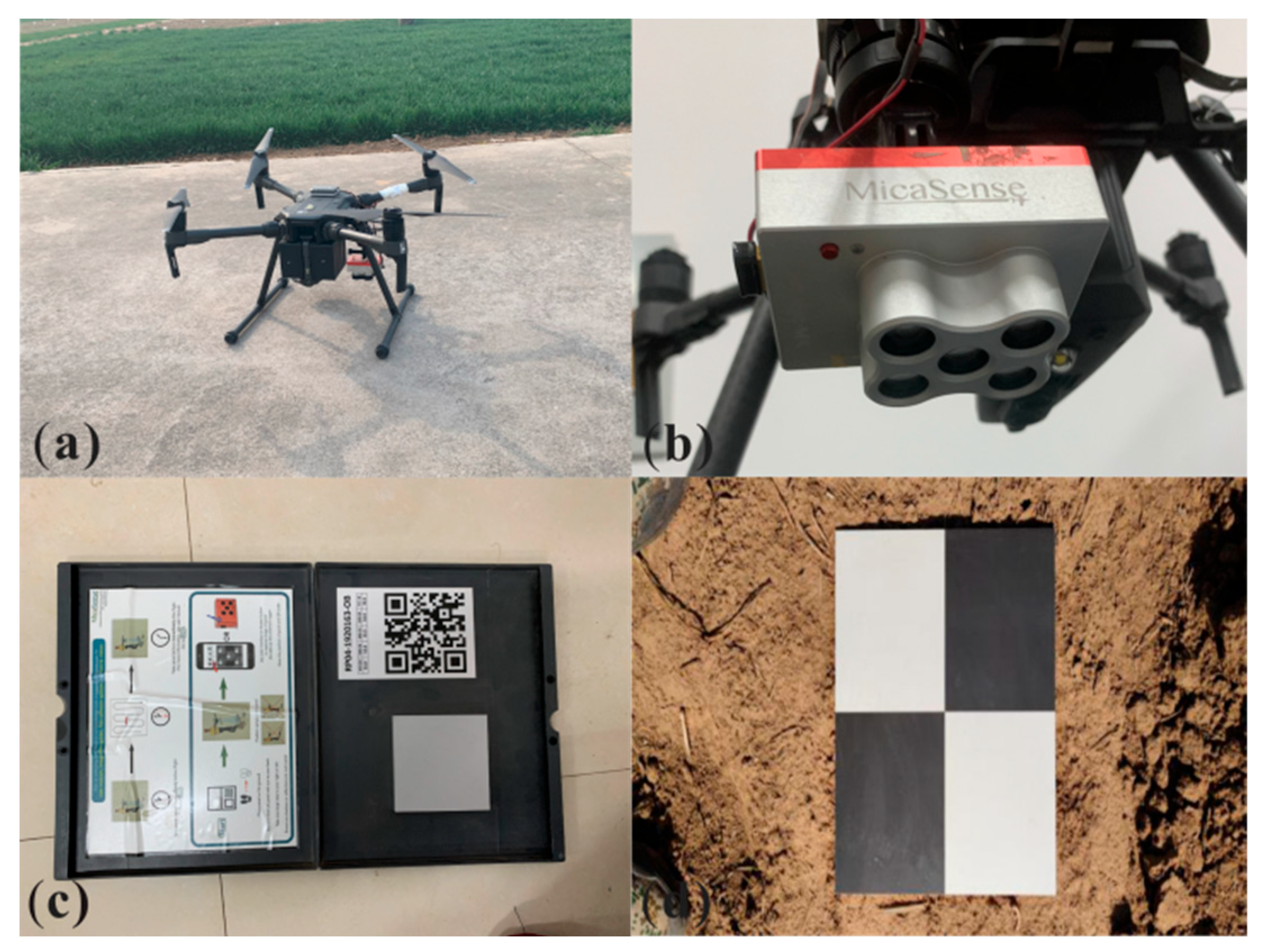
2.2. Spectral Data Acquisition and Processing

The spectral data used in the experiment were obtained from a DJI M210 equipped with the Micasense RedEdgeMX multispectral camera (Figure 2a,b). The DJI M210 is a four-axis multi-rotor vehicle with good stability and flight control, an average endurance of about 30 min, and a maximum horizontal flight speed of 18 m/s. The Red-Edge MX sensor on board the UAV captures five wavelength bands (red, green, blue, near-infrared, and red edge) with centre wavelengths of 668 nm, 560 nm, 475 nm, 840 nm, and 717 nm, respectively. The sensor has a resolution of 1280 × 960 for each band and a field of view of 47.2°. To account for possible cloud and light intensity variations during the mission, the multispectral camera is equipped with a radiometric calibration whiteboard (Figure 2c) and an on-board irradiance sensor, which are used for sensor calibration during post-image processing. The data used in the study were acquired at three fertility stages: heading stage, flowering stage, and filling stage, on 20 April, 6 May, and 26 May, respectively. The missions were flown between 11:00 a.m. and 2:00 p.m. to avoid shadow interference and at an altitude of 30 m with a heading overlap rate of 85% and a bypass rate of 80%. 12 ground control points (Figure 2d) were established for easy later geo-correction, and the sensors used a vertical ground plane with an equal time interval photo mode to collect data.

2.3. UAV Image Pre-Processing

In this study, multispectral data were collected at three different stages (T1, T2, and T3) of the crop growth cycle, corresponding to the heading, flowering, and filling periods, respectively. The collected data for each period was then transferred to a computer and imported into Pix4DMapper Pro software (version 4.4.12) (Pix4D S.A., Prilly, Switzerland), where three projects were created. Project parameters were set to align the images using a feature point-matching algorithm. First, a sparse point cloud of the flight area was generated from the UAV image and position data. A spatial grid was then created based on the sparse point cloud, and the spatial coordinate information of the 12 GCPs was added. Next, a sparse point cloud with precise positions was generated, and the surface geometry of the flight area was reconstructed. Finally, a high-resolution digital orthophoto (DOM) and a digital surface model (DSM) of the flight area were generated, and the processed images were exported as TIFF files. The multispectral HD digital orthophotography was divided into plots using ArcMap 10.5 (Environmental Systems Research, Inc., Redlands, CA, USA). A shapefile was created, divided into 180 plots with IDs corresponding to the number of each experimental plot. Using the Zonal Statistics as Table function in the ArcMap software (version 10.8), the average value of each plot was calculated for each of the five bands, and the five spectral bands corresponding to each plot were identified and exported.

2.4. Acquisition of Vegetation Index

Spectral reflectance alone cannot directly reflect the growth condition and health status of vegetation, as it is simply the ratio of the intensity of reflected light to the intensity of incident light from vegetation. However, vegetation indices can better reflect the growth condition and health status of vegetation by combining waveband information according to different spectral reflectances. Many vegetation indices have been widely used with high reproducibility and accuracy. In this study, we calculated 16 vegetation indices based on the UAV multispectral data we acquired for three fertility periods, which are sensitive to the yield of winter wheat. All feature information can be found in

Table 1. Information about the Vegetation Index.

Vegetation Index	Formulas	References	Applications
Normalised Difference Vegetation Index	$NDVI=(NIR-R)/(NIR+R)$	[28]	Agriculture, Vegetation
Normalised Difference Red-Edge	$NDRE=(NIR-RE)/(NIR+RE)$	[29]	Vegetation
Blue-normalised difference vegetation index	$BNDVI=(NIR-B)/(NIR+B)$	[30]	Vegetation
Green NDVI	$GNDVI=(NIR-G)/(NIR+G)$	[31]	Vegetation
Blue-wide dynamic range vegetation index	$BWDRVI=(0.1\ast NIR-B)/(0.1\ast NIR+B)$	[30]	Vegetation
Coloration index	$CI=(R-B)/R$	[32]	Vegetation
Transformed Vegetation Index	$TVI=\sqrt{NDVI+0.5}$	[33]	Vegetation
Wide Dynamic Range Vegetation Index	$WDRVI=(0.1\ast NIR-R)/(0.1\ast NIR+R)$	[34]	Vegetation
Green ratio vegetation index	$GRVI=NIR/G$	[35]	Vegetation
Red-Green Ratio	$RGR=R/G$	[36]	Vegetation
RedEdge Ratio Index 1	$RRI1=NIR/RE$	[29]	Remote sensing
RedEdge Ratio Index 2	$RRI2=RE/R$	[29]	Remote sensing
Soil and Atmospherically Resistant Vegetation Index	$\begin{array}{l}SARVI=2.5\ast (NIR-R)/\\ (1+NIR+6\ast R-7.5\ast B)\end{array}$	[37]	Soil, Vegetation
Adjusted transformed soil-adjusted Vegetation Index	$\begin{array}{l}ATSAVI=1.22\ast (NIR-1.22\ast R-1.22)/\\ (1.22\ast NIR+R-1.22\ast 0.03+0.08\ast (1+{1.22}^2))\end{array}$	[38]	Soil, Vegetation
Chlorophyll Index Green	$CI\mathrm{g}=(NIR/G)-1$	[33]	Vegetation
Chlorophyll IndexRedEdge	$CI\mathrm{re}=(NIR/RE)-1$	[33]	Vegetation

.

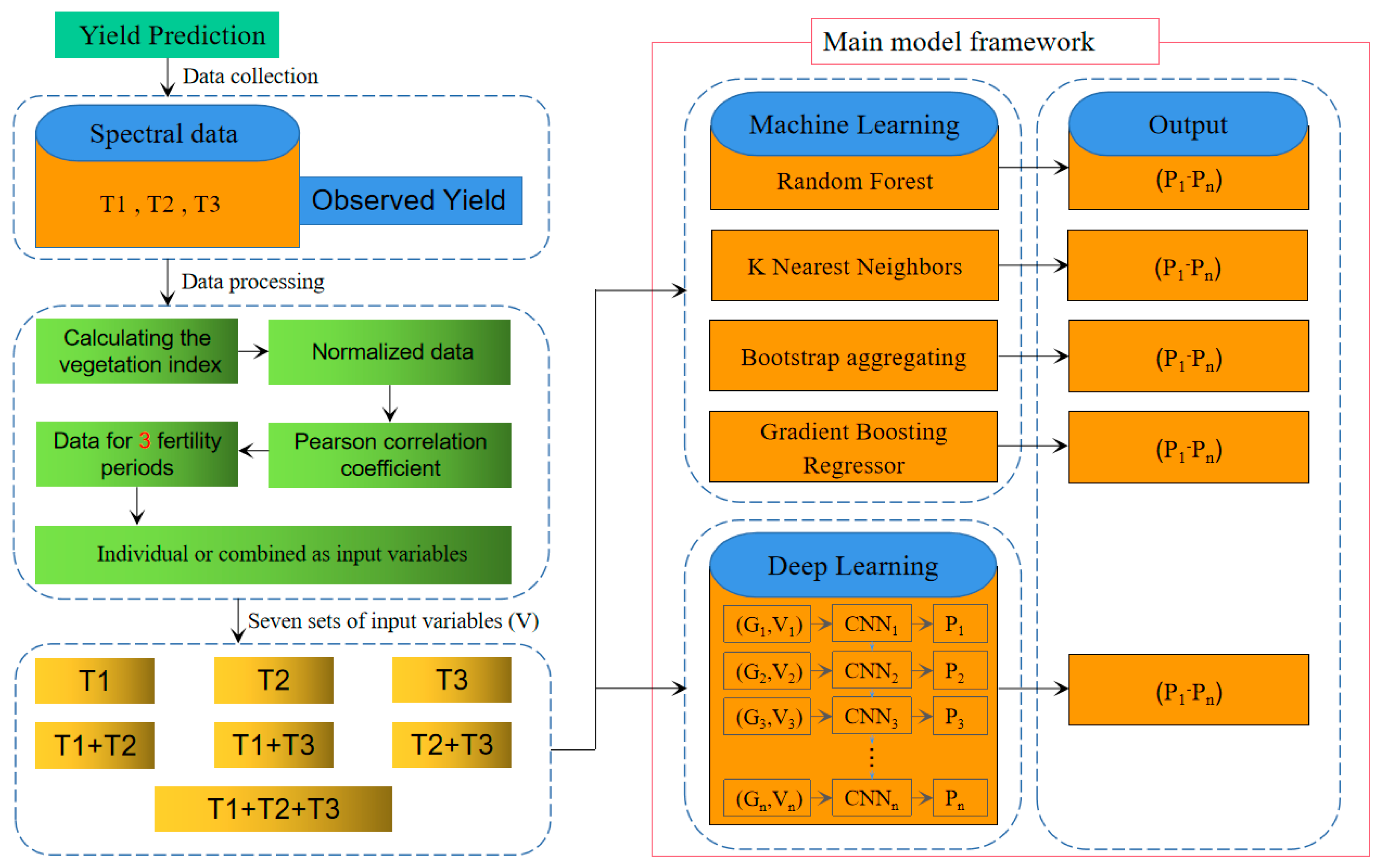
2.5. Framework for Yield Prediction Models

After obtaining the necessary data for this study, suitable deep learning and generalised machine learning models were selected to predict winter wheat yields (Figure 3). First, the multispectral vegetation index data collected during the three fertility periods were standardised, and the correlation between these indices and yield was analysed. In this study, minimum-maximum scaling is used to find the period maximum and minimum values for each feature, and the range of values of the data is scaled to between [0, 1] using the following formula:

$$x=(x-x_{\min })/(x_{\max }-x_{\min })$$

where x is the original data feature, x_min is the minimum value of the feature, and x_max is the maximum value of the feature.

Based on the correlation and significant characteristics of each vegetation index, all 16 vegetation indices constructed had a good correlation with yield and could be used as input variables for the predictive models. In addition, different combinations of fertility vegetation indices were investigated in the construction of the prediction model, and the three fertility vegetation index datasets were combined as input variables for the model based on the research needs. To evaluate the performance of the models, the input variables were randomly divided using a five-fold cross-validation method, where each fold was used as the validation set and the remaining four folds were used as the training set. All the acquired data were used as training and validation samples, and the final accuracy of the model was determined by calculating the mean value of the five results. Further details of the generalised machine learning and deep learning yield prediction models can be found in the flowchart. The yield prediction models were constructed using Python 3.8. In this study, grid search was chosen to screen the hyperparameters of the model by combining the defined hyperparameters and candidate values in a grid, also known as a Cartesian product, and then using cross-validation to evaluate the performance of each hyperparameter combination and selecting the best performing hyperparameter combination as the optimal combination to train the model to obtain the final model performance metrics.

2.5.1. Generalized Machine Learning Models

According to the results of previous research, we found that RF, KNN, GBR, Bagging, and CNN have shown the best predictive performance in prediction research in the field of agriculture, respectively, which is recognised by the public, so these five algorithms were chosen to construct yield prediction models in this study.

RF is an ensemble learning method based on decision trees. It works by constructing multiple decision trees, each trained with a random subset of features and datasets, and then combining the predictions of all the trees to obtain the final prediction [39,40,41]. RF is widely used in many machine learning applications due to its ability to automatically select features, handle high-dimensional data, and provide good robustness and interpretability.

KNN is a non-parametric regression algorithm based on distance metrics [42]. Its core idea is to predict the target value by finding the K nearest neighbours in the feature space. The performance of KNN depends on the choice of K value and the distance metric used. KNN works well with small datasets but can become less efficient when dealing with larger datasets [43].

GBR is an iterative integrated learning method that improves prediction performance by training multiple weak regression models and combining them [44]. GBR first trains a simple regression model, and then in each iteration, it trains a new regression model based on the error of the previous one. It then combines the output of all the models by weighting and averaging them to obtain the final prediction result, which is highly flexible and accurate [45].

Bagging is an integrated learning method based on the bootstrap sampling method. It trains multiple models by randomly sampling the training dataset and averaging their outputs to obtain the final prediction [46]. Bagged regression is effective in reducing model variance and generalisation error and performs well on large datasets [47]. The sampling technique allows a sample to be resampled multiple times with a replacement.

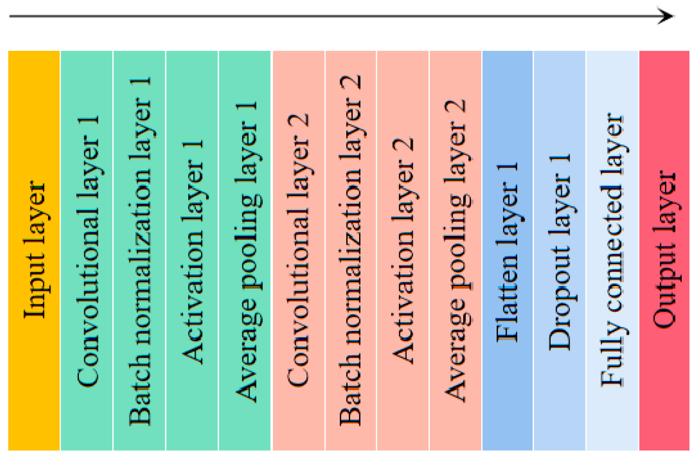
2.5.2. Deep Learning Models

A 1D CNN is a deep learning model based on convolutional operations and composed of several types of layers suitable for processing one-dimensional data [48]. The network typically includes an input layer, a convolutional layer, a pooling layer, a fully connected layer, a hidden layer, and an output layer, along with additional hidden layers such as batch normalisation, activation functions, and dropout. The convolutional layer is the core layer that extracts features from the input data by performing convolutional operations and contains a convolutional kernel whose size is usually a positive integer. In addition, the convolutional layer contains N filters of the same size. Pooling is used to reduce the dimensionality of the features in a 1D CNN, which reduces computational complexity and improves network robustness while preventing overfitting [49]. In a 1D CNN, the pooling layer typically follows the convolutional layer. The fully connected layer is a common neural network layer used to map the network output into a specific output space. Every neuron in a fully connected layer is connected to all the neurons in the previous layer. The batch normalisation layer is an optimisation method that normalises the input data of each batch, which speeds up the training process of the network. The activation function layer maps the linear output of the neural network into a non-linear space, which improves the performance of the network [50]. In a 1D CNN, the Dropout layer is a regularisation method used to prevent overfitting by randomly dropping a percentage of neurons in the network [51].

In this study, we constructed a 1D CNN model to predict winter wheat yield. The model architecture consists of 1 input layer, 2 convolutional layers, 2 batch normalisation layers, 2 activation function layers, 1 flattening layer, 1 dropout layer, 2 average pooling layers, 1 fully connected layer, and 1 output layer, as shown in Figure 4. The input to the 1D CNN model is one-dimensional vegetation index data. The number of filters in the two convolutional layers is 2 and 4, respectively, and the size of the convolutional kernel is 3. The batch normalisation layer is used to normalise small batches of data and normalise the output to a standard normal distribution, which prevents overfitting of the model and improves computational speed. We added a dropout layer that randomly drops nodes to further reduce model overfitting. The pool size is set to 2 × 1 with a step size of 1. The activation function used for the two activation function layers is ReLU. The output layer is a fully connected, dense layer with 1 node.

2.6. Model Evaluation Indicators

In this study, we used Pearson’s correlation coefficient to assess the relationship between vegetation indices and yield at each fertility period. In addition, we used the coefficient of determination (R²) and the root mean square error (RMSE), which are commonly used indicators to evaluate the performance of regression models, to assess the accuracy of our prediction models. In general, a higher Pearson correlation coefficient indicates a stronger correlation between yield and vegetation index, while a larger R² value (closer to 1) indicates a better ability of the model to explain the data. A smaller RMSE (closer to 0) indicates a better predictive ability of the model, which means that there is less error between the observed and predicted values. The formula for calculating R² and RMSE is shown below:

$$r_{(X,Y)}=\frac{Cov(X,Y)}{\sqrt{Var(X)Var(Y)}}$$

(1)

where $Cov(X,Y)$ represents the covariance of $X$ and $Y$, $Var(X)$ is the variance of $X$, and $Var\left(Y\right)$ is the variance of $Y$.

$$R^2=1-\frac{{\displaystyle {\sum }_{i=1}^n{({\stackrel{⌢}{y}}_i-y_i)}^2}}{{\displaystyle {\sum }_{i=1}^n{(y_i-\overline{y})}^2}}$$

(2)

$$RMSE=\sqrt{\frac{{\displaystyle {\sum }_{i=1}^n{({\hat{y}}_i-y_i)}^2}}{N}}$$

(3)

where $y_i$ is the observed value, ${\hat{y}}_i$ is the predicted value, $\overline{y}$ is the mean of the observed values, and N is the sample size.

3. Results

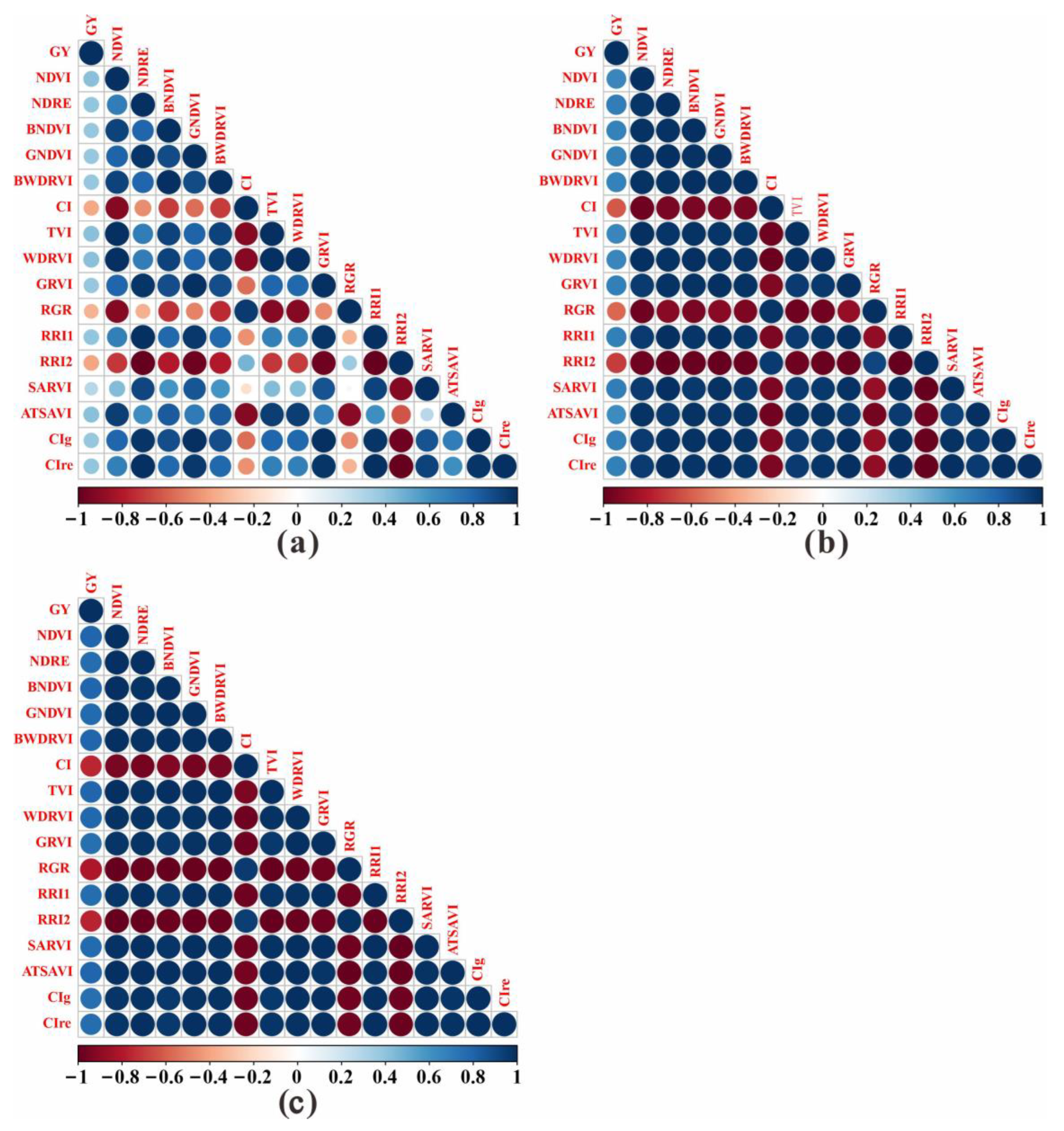
3.1. Correlation Analysis and Acquisition of Input Variable Sets

In this study, we selected 16 vegetation indices that showed a significant correlation with yield (Figure 5) and analysed the relationship between yield and the vegetation index variables of the three fertility periods in an integrated manner using a correlation matrix. The upper triangle of the matrix shows the correlation coefficients between yield and each of the 16 vegetation indices, while the lower triangle shows the amount of change in the correlation between yield and the 16 vegetation indices. As shown in Figure 5, it was observed that the correlation between yield and each vegetation index increased as the fertility stage of winter wheat progressed from the heading stage to the filling stage. ATSAVI and WDRVI had the best correlation with yield at the heading stage (Figure 5a), both reaching a value of 0.42, followed by NDVI, NDRE, TVI, RRI1, RRI2, and CIre, all with absolute correlation values with yield above 0.4. During flowering (Figure 5b), the correlation between vegetation indices and yield increased, except for RGR, which had an absolute correlation value of 0.58. The correlation between all vegetation indices and yield was above 0.62, with SARVI showing the best correlation with yield at 0.7. During the filling stage (Figure 5c), the correlation between vegetation indices and yield increased significantly, with absolute values above 0.76. CI, RGR, and RRI2 of the 16 vegetation indices showed a negative correlation with yield, while the rest of the vegetation indices showed a positive correlation with yield.

The multispectral features acquired at different fertility periods are complementary, and the sensitivity of vegetation indices constructed based on the reflectance of different spectral bands of the multispectral spectrum at different fertility periods varies. By analysing the spectra of different fertility periods, the complementarity between the spectra can be used to improve the accuracy of UAV remote sensing monitoring. Therefore, in this study, the vegetation indices of three fertility periods were used as input variable groups, and then the vegetation indices of two fertility periods were combined to obtain a total of seven input variable groups: (a) T1; (b) T2; (c) T3; (d) T1 and T2; (e) T1 and T3; (f) T2 and T3; (g) T1, T2, and T3.

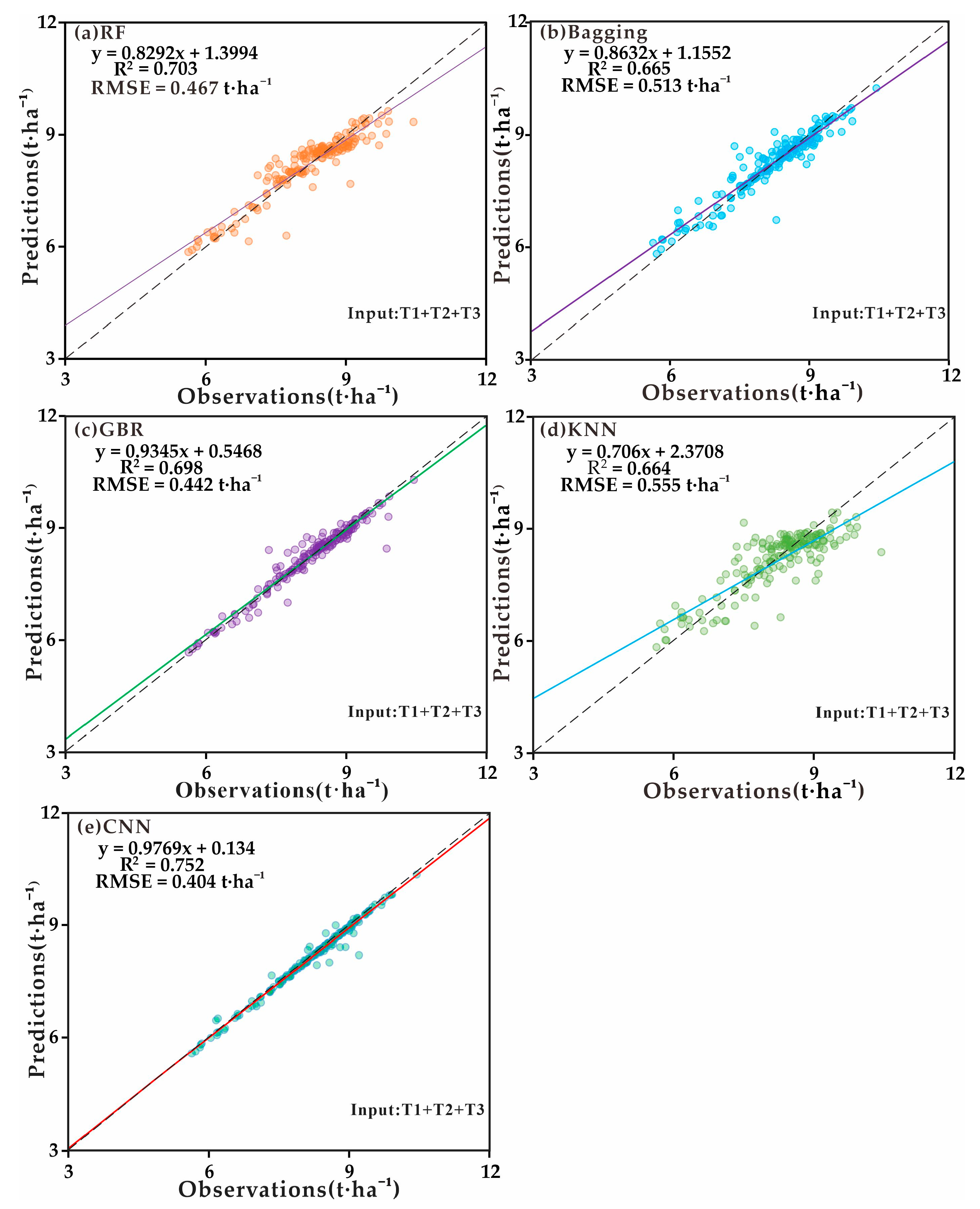
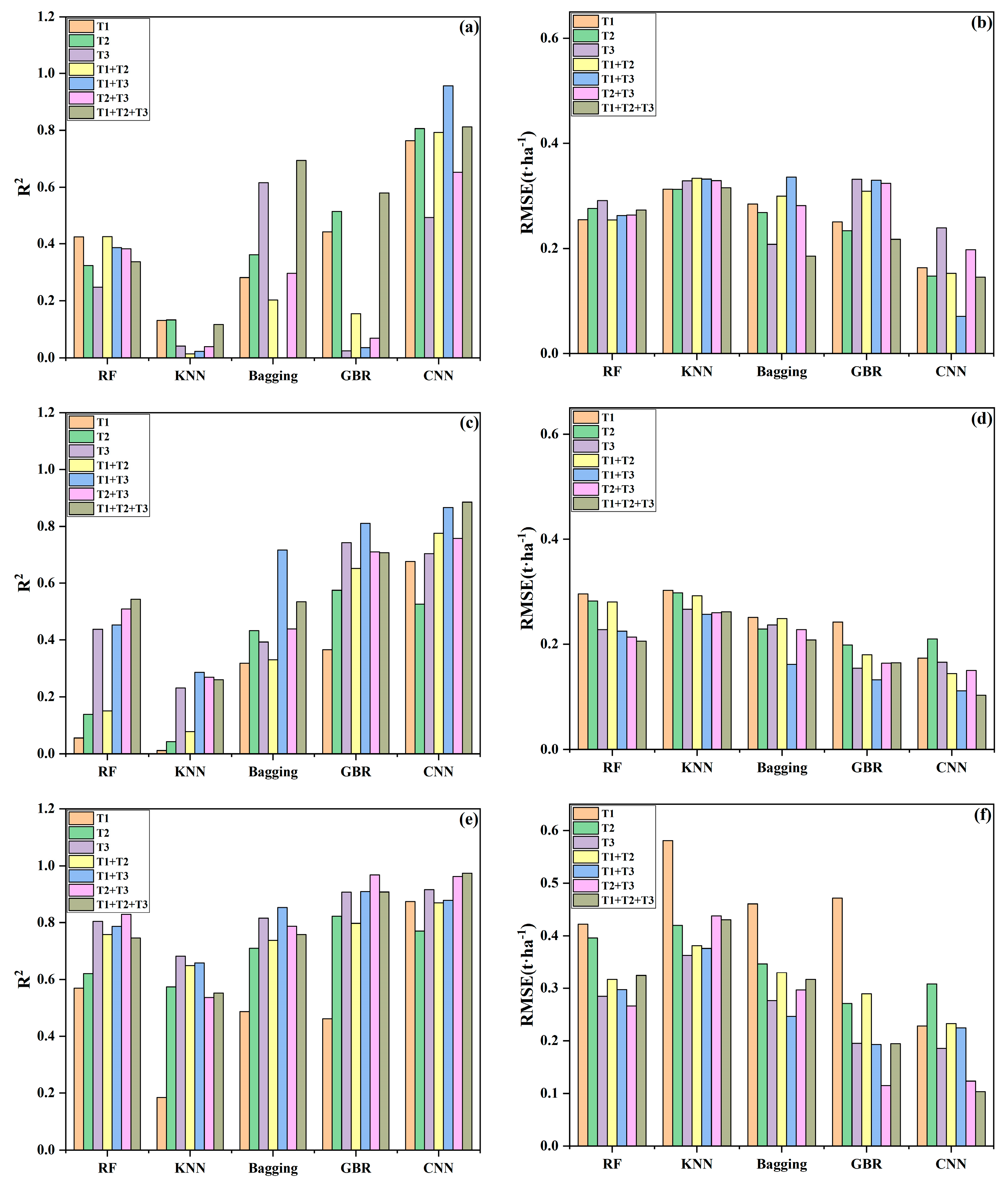
3.2. The Performance of Five Models on Yield Prediction

The RF model had the highest R² of 0.703 for input variable group g (T1, T2, and T3) (Figure 6); however, the lowest RMSE of 0.409 t·ha⁻¹ for input variable group f (T2 and T3) (

Table 2. Yield prediction model accuracy ((a) T1; (b) T2; (c) T3; (d) T1 and T2; (e) T1 and T3; (f) T2 and T3; (g) T1, T2, and T3).

Variable Sets	RF		Bagging		GBR		KNN		CNN		Means
	R2	RMSE (t·ha−1)	R2	RMSE (t·ha−1)	R2	RMSE (t·ha−1)	R2	RMSE (t·ha−1)	R2	RMSE (t·ha−1)	R2	RMSE (t·ha−1)
(a)	0.458	0.593	0.384	0.711	0.397	0.842	0.377	0.672	0.472	0.733	0.418	0.710
(b)	0.506	0.623	0.505	0.566	0.494	0.676	0.469	0.695	0.540	0.654	0.517	0.643
(c)	0.614	0.500	0.594	0.556	0.601	0.586	0.589	0.602	0.627	0.526	0.605	0.554
(d)	0.594	0.513	0.554	0.643	0.546	0.735	0.509	0.764	0.636	0.497	0.568	0.630
(e)	0.648	0.477	0.632	0.662	0.647	0.648	0.615	0.677	0.674	0.445	0.643	0.582
(f)	0.681	0.409	0.641	0.516	0.673	0.560	0.649	0.477	0.720	0.442	0.673	0.481
(g)	0.703	0.467	0.665	0.513	0.698	0.442	0.664	0.555	0.752	0.404	0.697	0.476
Means	0.611	0.512	0.568	0.595	0.579	0.641	0.553	0.635	0.631	0.529

). In general, R² increased as the number of input variables increased, and RMSE tended to decrease before increasing, as shown in Figure 6. However, except for input variable group d (T1 and T2), where the prediction accuracy was lower than that of input variable group c (T3), the inclusion of too many input variables had a negative impact on the prediction accuracy of the RF model.

The KNN model showed the highest yield prediction R² of 0.664 (Figure 6) for the input variable group g (T1, T2, and T3) and the lowest RMSE of 0.477 t·ha⁻¹ for input variable group f (T2 and T3) (Table 2). However, the RMSE was higher for both input variable groups d (T1 and T2) and e (T1 and T3) with larger errors, indicating that the combination of two fertility data sets had an effect on the predictions of the KNN model.

The Bagging model gave the highest yield prediction accuracy (R² = 0.665, RMSE = 0.513 t·ha⁻¹) for input variable group g (T1, T2, and T3) (Table 2). While input variable group d (T1 and T2) had a higher R² than input variable groups a (T1) or b (T2), its RMSE was higher than input variable group b (T2) (RMSE = 0.566 t·ha⁻¹), indicating a larger error. Similarly, input variable group e (T1 and T3) had a higher R² than input variable groups a (T1) or b (T3), but its RMSE was higher than that of input variable group b (T3) (RMSE = 0.556 t·ha⁻¹), indicating that increasing the number of input variables also negatively affected the predictive accuracy of the Bagging model.

The GBR model produced a maximum R² and minimum RMSE of 0.698 and 0.442 t·ha⁻¹ for input variable group g (T1, T2, and T3), respectively (Table 2). It can be observed that the accuracy of the model gradually improved with increasing fertility, with the highest accuracy at input variable group c (T3), where R² improved to 0.601 and RMSE reduced to 0.586 t·ha⁻¹, as input variable groups progressed from a (T1), b (T2), or c (T3). However, input variable groups d (T1 and T2) or e (T1 and T3) both had a higher RMSE than variable group c (T3), indicating that combining two fertility data sets as input features to the GBR model resulted in a larger error (Figure 6).

As for the CNN model, the best yield prediction accuracy (R² = 0.752, RMSE = 0.404 t·ha⁻¹) was obtained for the input variable group g (T1, T2, and T3) (Table 2). In general, the R² of the CNN model increased with increasing input variables, and the RMSE gradually decreased, indicating a gradient improvement in the accuracy of the model (Figure 6).

The mean values of R² and RMSE were calculated for different input variable groups to observe the predictive performance of different models (Table 2). The mean value of R² for input variable group g (T1, T2, and T3) was the highest at 0.697, and the mean value of RMSE was also the lowest at 0.476 t·ha⁻¹ (Table 2). In conclusion, all five models had the best prediction accuracy for input variable groups g (T1, T2, and T3), and the CNN models obtained the best model accuracy for different input variable groups. The average accuracy of the five models based on different input variable groups was then calculated (Table 2). It was found that the average ranking of the predicted R² for each model was: CNN > RF > GBR > Bagging > KNN, and the mean ranking of the predicted RMSE for each model was: CNN < RF < Bagging < KNN < GBR. The CNN model was still found to have the best accuracy, with the RF model having the second-best accuracy. The GBR model had the largest RMSE and produced a larger error. By comparing the RMSEs under different input variable groups, it was found that larger errors were produced under input variable groups a (T1) or b (T2) with RMSEs of 0.842 t·ha⁻¹ and 0.676 t·ha⁻¹, respectively, indicating the poor performance of GBR in predicting individual early fertility stages of winter wheat, as also evidenced by the RMSEs for input variable groups d (T1 and T2). Thus, RF was shown to be a suitable generalised machine learning model when different-sized input variable groups were considered to construct the prediction model, while the prediction performance of the deep learning CNN model was shown to be superior to that of the machine learning models.

In summary, both the generalised machine learning-based model and the deep learning model obtained the best prediction accuracy with the input (g) combination of variables as shown in

Table 3. Accuracy of each irrigation treatment for the optimal yield prediction model.

Treatment	RF		Bagging		GBR		KNN		CNN
	R2	RMSE (t·ha−1)	R2	RMSE (t·ha−1)	R2	RMSE (t·ha−1)	R2	RMSE (t·ha−1)	R2	RMSE (t·ha−1)
IT1	0.256	1.05	0.553	0.531	0.552	0.556	0.411	0.811	0.684	0.917
IT2	0.732	0.201	0.61	0.299	0.605	0.232	0.538	0.207	0.543	0.642
IT3	0.345	0.381	0.547	0.269	0.573	0.252	0.614	0.416	0.682	0.446
IT4	0.459	0.309	0.724	0.144	0.795	0.148	0.663	0.242	0.735	0.464
IT5	0.827	0.207	0.655	0.368	0.514	0.392	0.726	0.626	0.62	0.496
IT6	0.337	0.474	0.612	0.473	0.706	0.309	0.673	0.425	0.902	0.59

. It was found that the RF, Bagging, GBR, KNN, and CNN models obtained the highest accuracy at IT5, IT4, IT4, IT5, and IT6, respectively, indicating that the models were more capable of predicting yield under moisture deficit conditions and were more suitable for yield prediction.

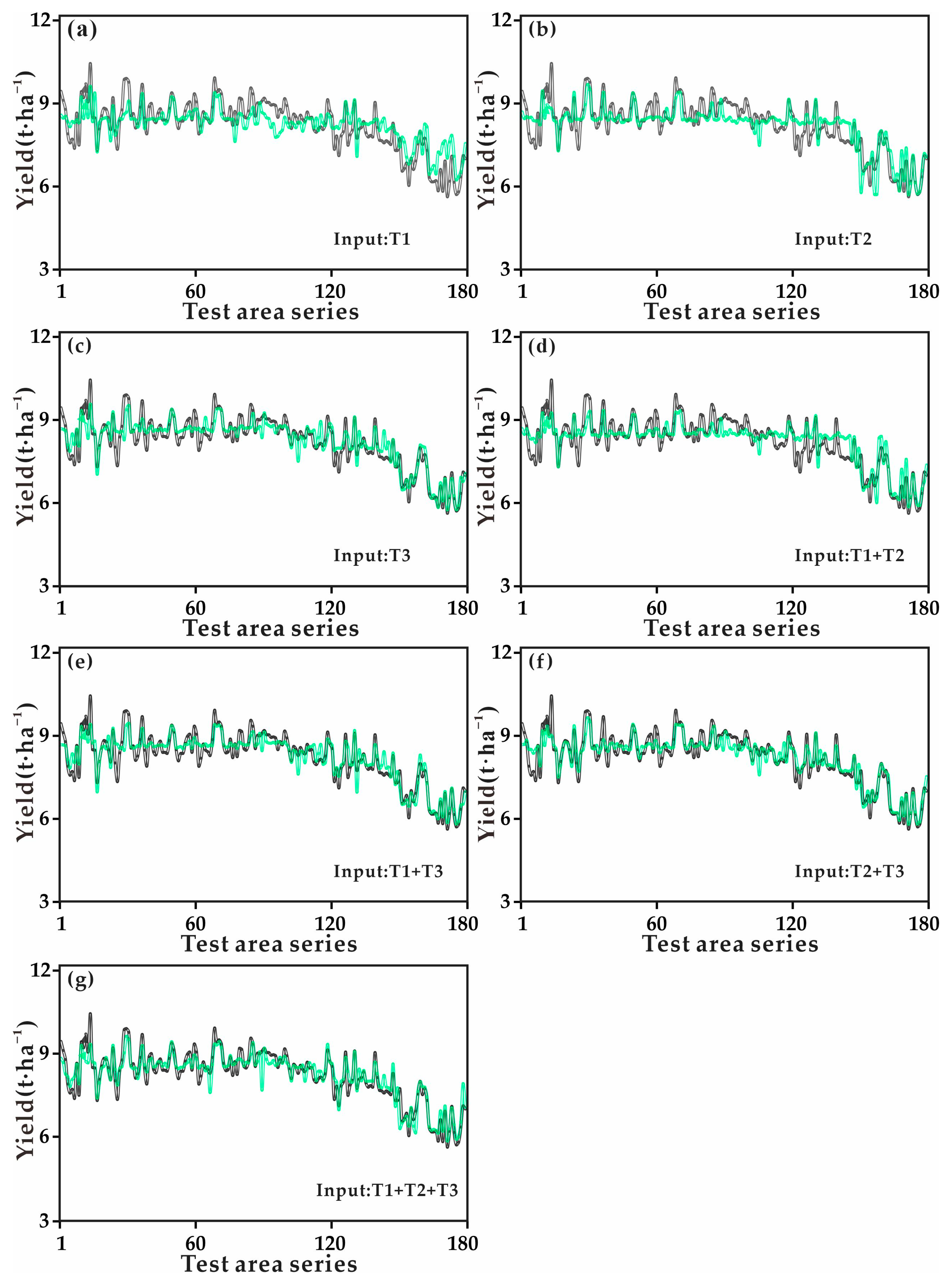
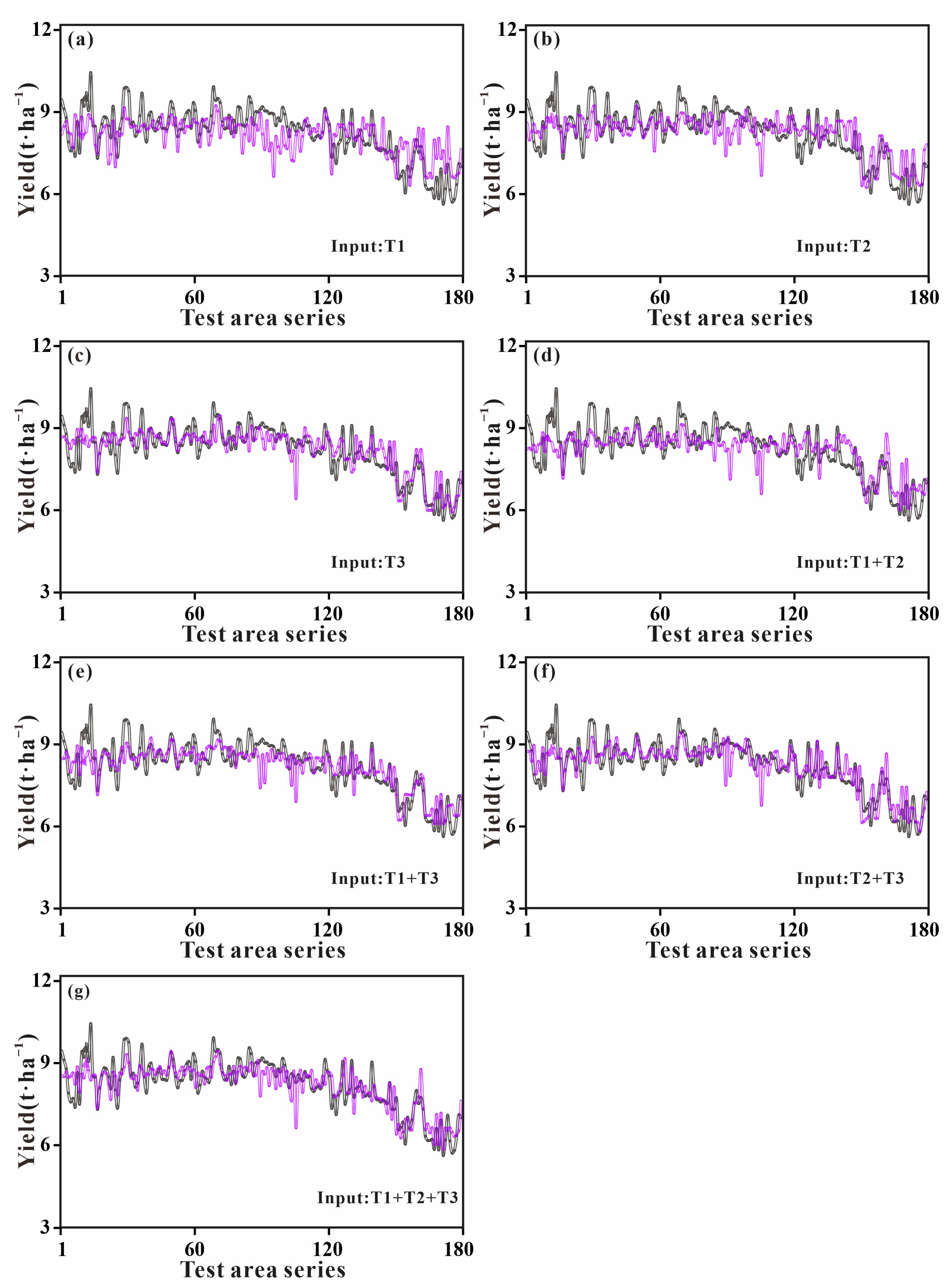
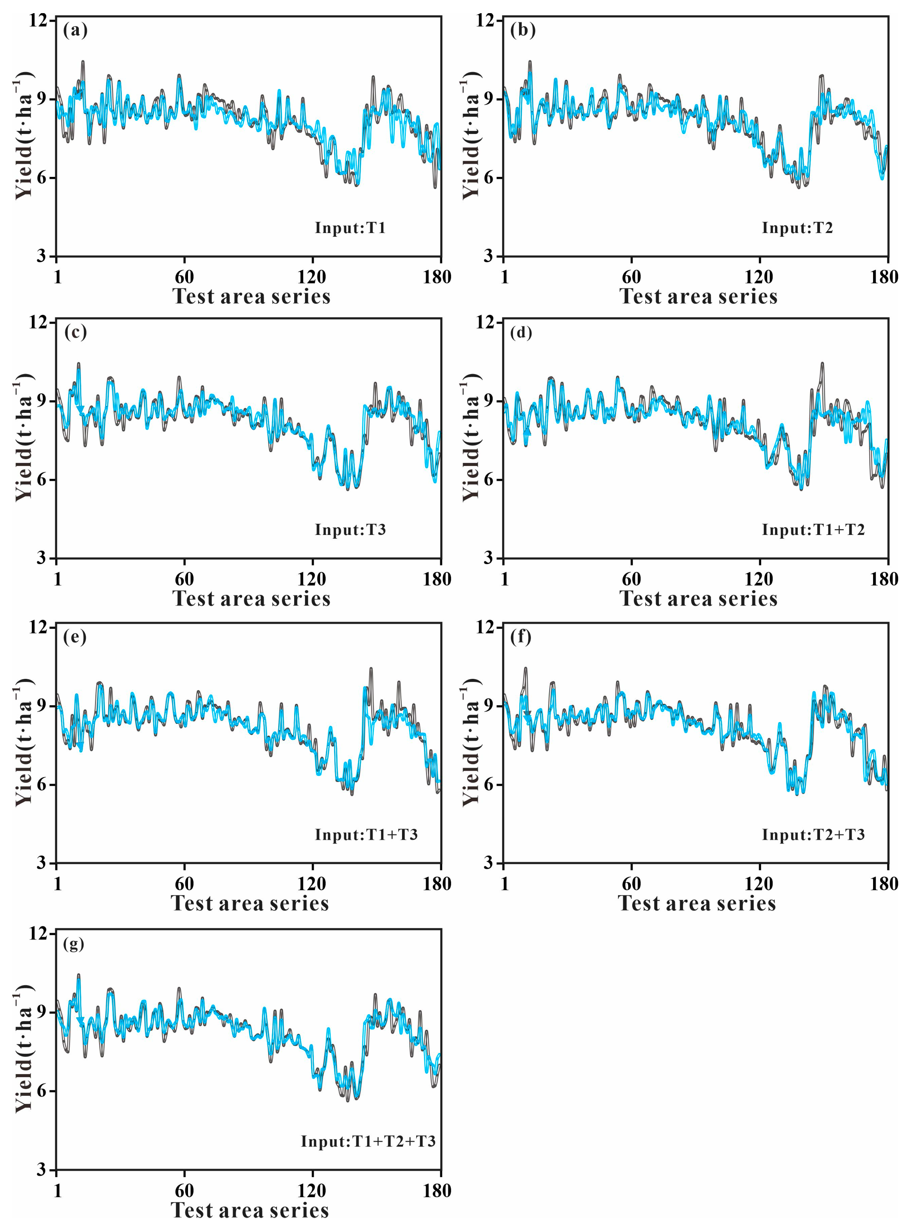
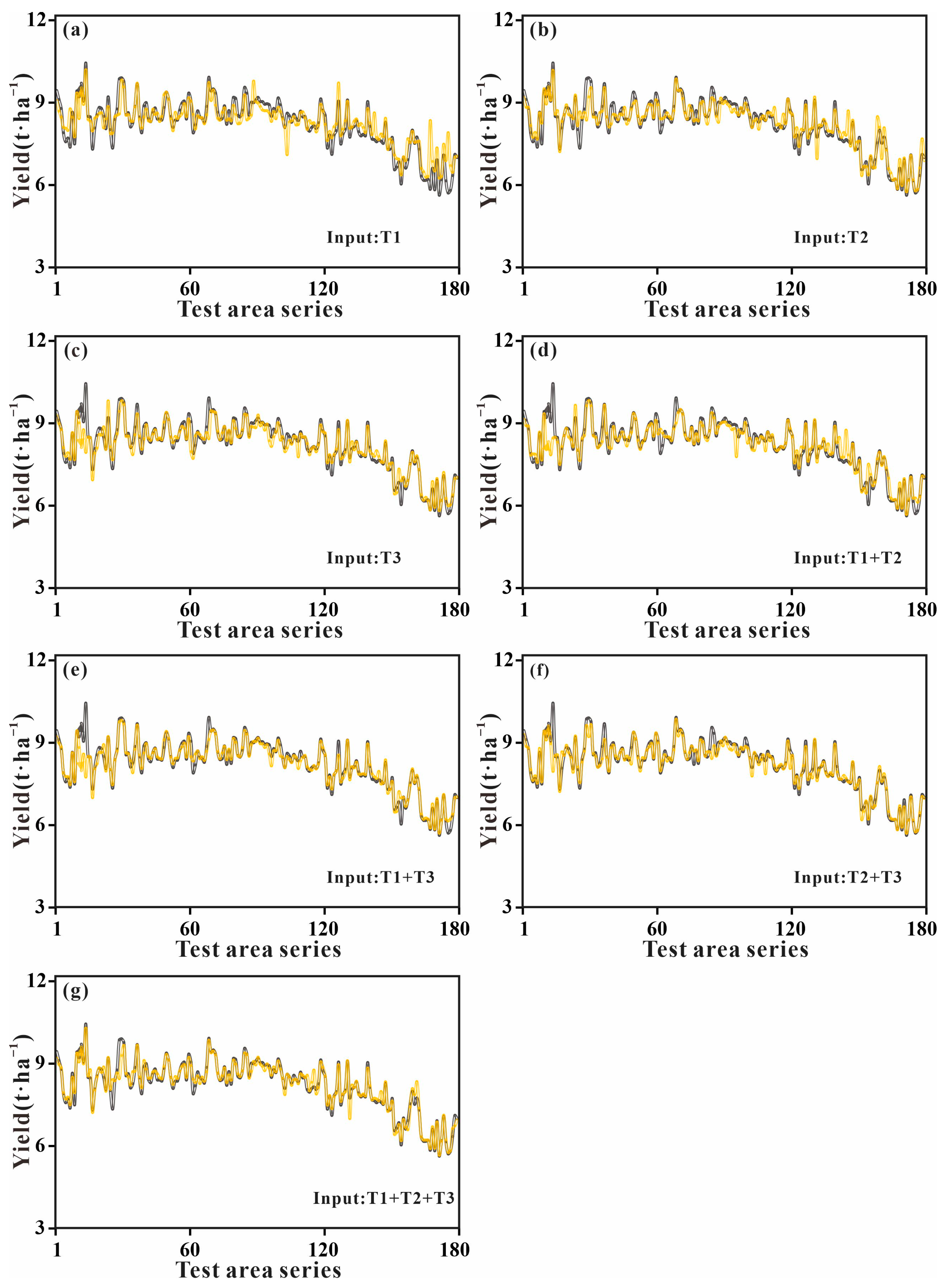
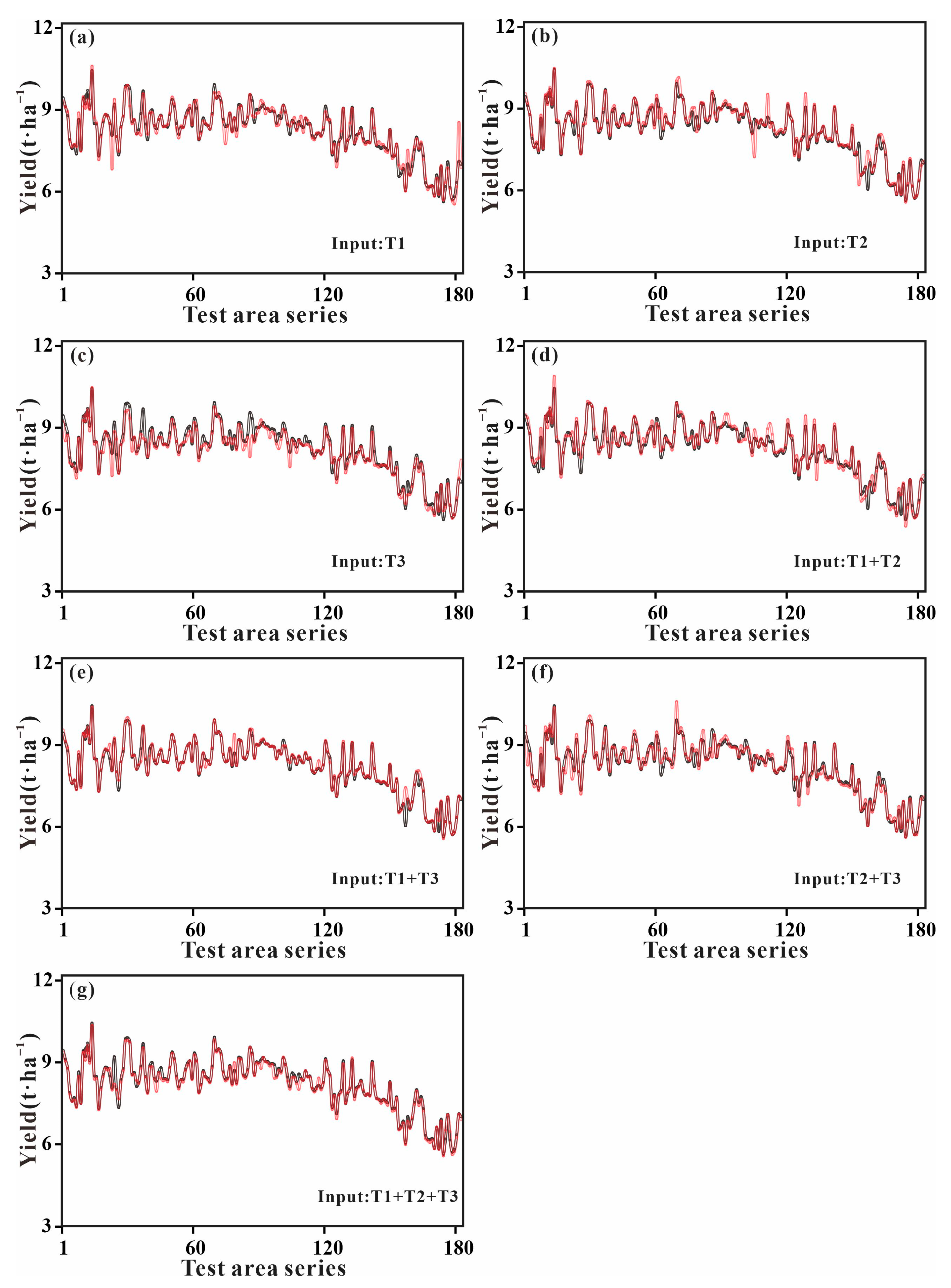
3.3. Analyzing the Dynamics of Predicting Yield

The different models did not consistently predict winter wheat yield dynamics, especially for wheat under different treatments (Figure 7, Figure 8, Figure 9, Figure 10 and Figure 11). The RF, KNN, and GBR models predicted significantly lower yield values than observed values in the range of 1–120 plots (IT1, IT2, IT3, and IT4) and significantly higher yield values in the range of 121–180 plots (IT5 and IT6). In addition, the RF model predicted higher yield values for input variable group d (T1). The Bagging model showed less volatility and fluctuated within the range of 1–180 plots. The CNN model outperformed the other prediction models in terms of yield prediction under different irrigation treatments, regardless of the variation in the input variable groups.

To evaluate the dynamic prediction performance of yields in different yield ranges, the observed yield data were divided into three groups: the upper quartile (observed yield > 8.865 t·ha⁻¹), the middle quartile (7.745 t·ha⁻¹ < observed yield < 8.865 t·ha⁻¹), and the lower quartile (observed yield < 7.745 t·ha⁻¹). Analyzing the variation of R² and RMSE for the five models (Figure 12), the CNN model showed the best prediction performance when the observed yield was below 7.745 t·ha⁻¹, except for the input variable group (b). The generalised machine learning model, GBR, performed second best and showed good yield prediction performance, except for the input variable group (a). The RF, KNN, and Bagging models, although not showing the best prediction performance, also showed good prediction performance when predicting lower observed yields. Therefore, the CNN model is more suitable for predicting lower observed yields, while the GBR is the most suitable generalised machine learning model for predicting lower observed yields.

The CNN showed the best prediction performance for observed yields between 7.745–8.865 t·ha⁻¹, except for input variable groups (b) and (c), while the GBR had the second-best prediction performance. The CNN model achieved the lowest RMSE of 0.103 t·ha⁻¹ for the input variable group (g). Therefore, the CNN model is more suitable for predicting observed yields in the middle range of the data.

For observed yields > 8.865 t·ha⁻¹ (quadratic precision plots c and d), the CNN model had the highest R² for the input variable group (g) and the lowest RMSE for the input variable group (e) among the CNN models. Among the generalised machine learning models, the GBR showed better prediction performance for input variable groups (a), (b), and (g); the Bagging model showed better prediction performance for input variable group (c); and the RF model showed better prediction performance for input variable groups (d), (e), and (f).

Overall, the CNN models showed the best prediction performance for different observed yield ranges based on most input variables and can be used to predict yields in different ranges of winter wheat. In addition, the generalised machine learning models showed good prediction performance at lower observed yields, with the second-best prediction performance in the medium yield range and unsatisfactory prediction performance at higher observed yields. This suggests that the generalised machine learning models are not suitable for predicting higher observed yields (observed yields > 8.865 t·ha⁻¹).

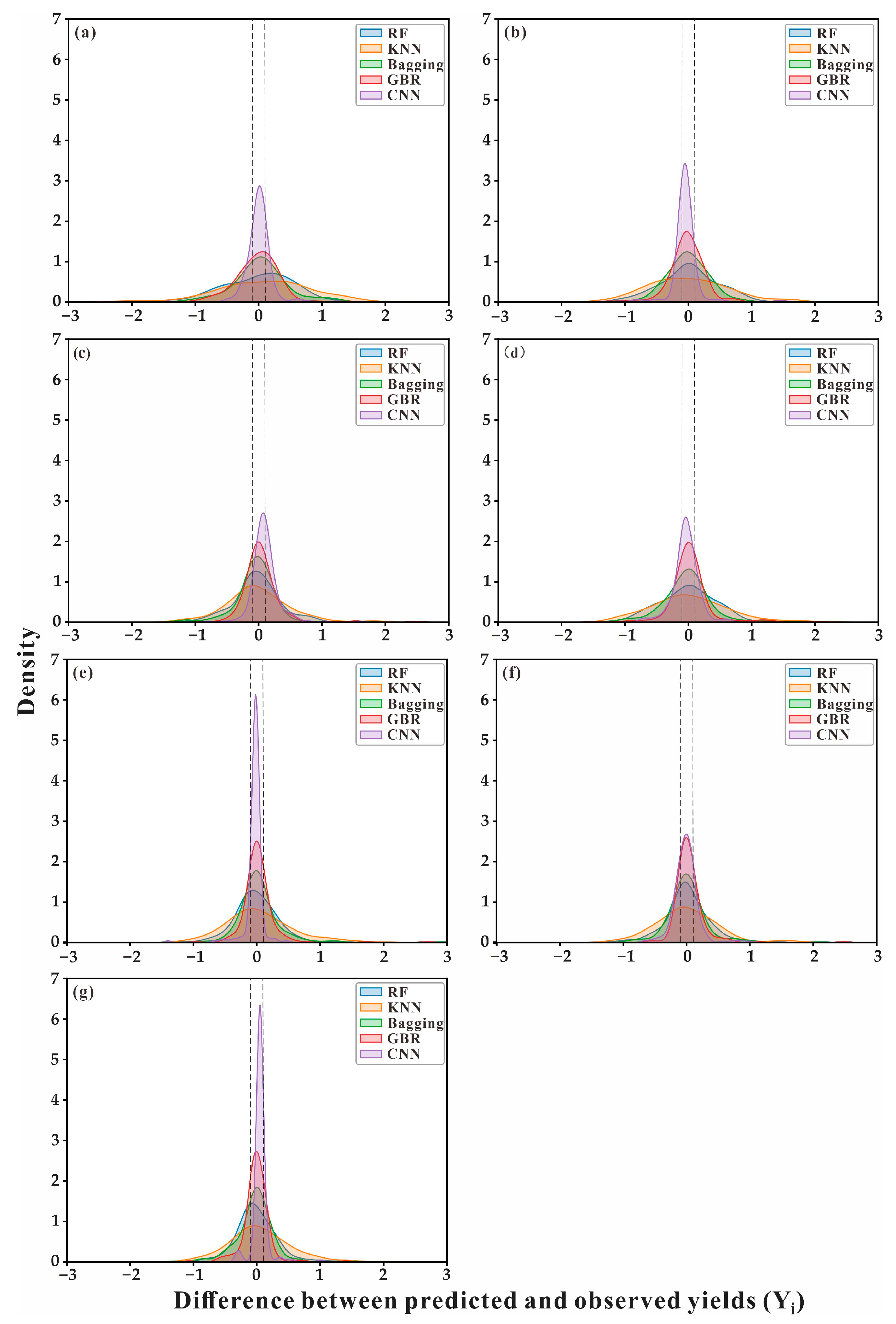
3.4. Distribution of Differences between Observed and Predicted Yields

This study shows the distribution of differences between predicted and observed yields (Y_i = observed yield value-predicted yield value) for different groups of variables and models (Figure 13). The Y_i density of the generalised machine learning models increased significantly in the range of −0.1 to 0.1 t·ha⁻¹ as the wheat growth stage progressed when using individual fertility data as input variables. In input variable group (c), the GBR model had a significantly higher Y_i density (48.89%) than the RF (27.22%), KNN (20%), and Bagging (35%), with the CNN model at 52.22%, all higher than the generalised machine learning model. In input variable group (e), the deep learning model (88.89% for CNN) had a significantly higher kernel density between −0.1 and 0.1 t·ha⁻¹ than the generalised machine learning models (27.78% for RF, 20.26% for KNN, 45.56% for Bagging, and 66.11% for GBR). For the input variable group (g), the deep learning model (82.78% for CNN) also had higher Y_i densities in both the −0.1 and 0.1 t·ha⁻¹ ranges than the generalised machine learning models (28.89% for RF, 23.89% for KNN, 41.67% for Bagging, and 60% for GBR). Mean values of Y_i densities were calculated for different sets of input variables and models, and the deep learning models (66.27% for CNN) showed significantly better Y_i densities in the range of −0.1 and 0.1 t·ha⁻¹ ranges than the generalised machine learning models (26.19% for RF, 17.06% for KNN, 35.47% for Bagging, and 50.32% for GBR). In summary, the deep learning models outperformed the generalised machine learning models for all prediction models constructed using different numbers of input variables, and the CNN models were closer to the actual values.

4. Discussion

Winter wheat yield trends show variability over time and are influenced by various factors such as water availability, climate conditions, soil type, geographical region, and the growing demand for grain production to feed a growing population. Predicting future wheat yield trends is a challenging task. In this study, 16 multispectral vegetation indices were selected as input variables for yield prediction models that have high yield sensitivity during the heading, flowering, and filling stages. Instead of using multispectral band reflectance directly, vegetation indices were preferred as input variables because they are widely used to study vegetation growth status and change and have high application value and accuracy. The absolute values of the correlations between the vegetation indices selected for this study and yield gradually increased with the development of the reproductive period. At the filling stage, all the vegetation indices showed extremely strong correlations, with the absolute values of the correlations between NDVI, BNDVI, TVI, RGR, and ATSAVI all reaching more than 0.8, which is consistent with the findings of Jewan [52]. The yield prediction model constructed from the vegetation indices of a single fertility period showed that the higher the correlation between vegetation indices and yield, the higher the accuracy of the constructed model. The correlation between vegetation indices and yield at the filling stage was above 0.7, and the maximum value of R² of the model reached 0.627, which is larger than the maximum R² of 0.472 of the model at the heading stage, consistent with the findings of Bian [15]. These results indicate that the best predictions for individual growth stages occur at the filling stage. It is also noteworthy that the correlation between ATSAVI and yield was poor at 0.289 at the heading stage but above 0.7 at both the flowering and filling stages. This may be due to the limited canopy cover of wheat at the heading stage, where spectral reflectance is disturbed by background factors such as bare soil, resulting in a low correlation with the constructed vegetation index.

Generalised machine learning models are widely used in precision agriculture, particularly in predicting phenotypic information about crops, such as crop yield [53]. This study shows that generalised machine learning models are not only influenced by different crop fertility periods but also by the number of input variables. Overall, the RF model showed the best prediction performance among the four generalised machine learning models, while the KNN model showed the worst performance. As shown in the accuracy table, when a single fertility vegetation index was used as an input variable for three fertility periods, the RF model improved the mean R² value by 6.36%, 5.75%, and 10.04% compared to the Bagging, GBR, and KNN models, respectively. When two fertility vegetation indices were used as the input variable set, the RF model had mean R² values of 5.3%, 3.09%, and 8.5% higher than the Bagging, GBR, and KNN models, respectively. However, the GBR model outperformed the RF model in predicting yield and observed yield when the range 8.865 t·ha⁻¹ > observed yield > 7.745 t·ha⁻¹ was considered. The GBR model also showed good accuracy in the range of observed yield > 8.865 t·ha⁻¹. This is probably due to the fact that this experiment included six irrigation treatments and the data distribution had some regularity, resulting in a high accuracy of the regression between the model predicted and observed values (Fig.). RF models are often able to capture non-parametric or non-linear relationships between predictors or yields and input variables, making their predictions more stable and reliable. Therefore, the RF model is a more desirable model for yield prediction in generalised machine learning models [54]. In his study, Zhong found that the R² of both the RF model and the Bagging model was above 0.91; however, the error of the RF model was lower than that of the Bagging model [55]. In a study to predict the yield of alfalfa in the current season, Feng showed that the accuracy of the RF model was better than that of the KNN model, and the R² of both models was above 0.8 [53]. However, in our study, the mean R² of the RF model was 7.57%, 5.43%, and 10.49% higher than that of the Bagging, GBR, and KNN models, respectively. The mean R² values were in the range of 0.55–0.62, indicating that the GBR model outperformed the Bagging and KNN models. This highlights that the prediction accuracy of generalised machine learning models is affected by different application scenarios and datasets.

In this study, both generalised machine learning models and CNN models from deep learning were used to predict winter wheat yield. The CNN model showed the best prediction performance for all seven sets of input variables, ranging from single fertility data as input variables to a combination of three fertility data as input variables. Compared to the best-performing generalised machine learning model with the same combination of inputs, the R² of the CNN model improved by 3.11%, 6.6%, 2.08%, and 6.91%, respectively. These results are consistent with Ghanbari [56], who found in his study on sediment core size mapping that the CNN model outperformed the best RF model in the generalised machine learning model in terms of prediction performance. When the observed yield was <7.745 t·ha⁻¹, each generalised machine learning model showed better prediction accuracy, and overall, the CNN model still had the best prediction performance. These results are consistent with those of He [57], who found similar results when predicting the minimum greenhouse temperature, both showing that the deep learning model had the best prediction performance among the machine learning models. In their study on winter wheat yield prediction, Tanabe [25] found that the CNN model they constructed outperformed the linear regression model and performed best at the heading stage, which was considered to be the most appropriate data collection stage for winter wheat. However, our experimental results showed that the prediction accuracy of the model was better at the filling stage than at the heading and flowering stages, indicating that the results of the prediction model may be influenced by the variety of winter wheat, the region, the climate, and the experimental conditions. Srivastava [58] analysed the performance of machine learning and deep learning methods in winter wheat yield prediction and found that the CNN model outperformed all other baseline models (with a 7–14% reduction in RMSE), which was also demonstrated in our study. However, the reduction in RMSE of the CNN model varied from 1.44–18.77%, further illustrating that the performance of the prediction models in winter wheat yield prediction is influenced by a number of factors.

This experiment suggests that the RF, KNN, and GBR models underestimate yield in the 1–120 plot range and overestimate yield in the 121–180 plot range. Furthermore, for the 4 irrigation treatments IT1, IT2, IT3, and IT4 in the 1–120 plot range, it is shown that the RF, KNN, and GBR models underestimate yield for treatments with more than 40% adequate irrigation and overestimate yield for treatments with less than 40% adequate irrigation. In a separate study, He [59] also found that the spatial downscaling method for precipitation in an adaptive random forest underestimates extreme precipitation. This suggests that different experimental settings and machine learning methods may lead to over- or underestimation of monitoring metrics. The difference between observed and predicted yields, denoted as Y_i, reflects the accuracy of a model’s prediction. The smaller the value of Y_i, the closer the predicted yield value is to the observed yield value, and the better the model matches the actual situation. Hu [60] developed a yield prediction model based on a non-linear function that relates infrared water stress indicators to winter wheat yield. The error between the predicted yield values and the actual yield values was small, demonstrating the feasibility of the model in predicting yield. Our experiments showed that the CNN model constructed with seven input variables had the highest percentage, reaching up to 88.89% when Y_i was in the range of −0.1 and 0.1 t·ha⁻¹. However, the generalised machine learning model did not perform well in this error range, indicating that the CNN model had the best prediction accuracy as the error between its predicted yield values and the observed yield values was small. Nevertheless, the GBR model also improved the percentage of Y_i in the range of −0.1 and 0.1 as the input variable set data increased, achieving a maximum of 66.11%, thereby improving the prediction accuracy of the model. This result demonstrated the good predictive ability of the GBR model in the generalised machine learning model. Leng [61] demonstrated that in predicting and optimising the specific surface area of biochar, the nitrogen content of biochar, and biochar yield, the GBR model generally had better predictive ability than the RF model. Although the RF model slightly outperformed the GBR model in this study, the predictive ability of the GBR model was more stable in terms of the distribution of Y_i. This stability may be due to the fact that the GBR model automatically adjusts the error through continuous iteration during the training process, thereby reducing the influence of outliers on the results, resulting in high accuracy and generalisation ability for the GBR model.

In this study, only one deep learning model, CNN, was investigated. Future research will consider the inclusion of recurrent neural network models and long- and short-term memory network models for yield prediction. In addition, this study only used UAV multispectral data to construct vegetation indices as input variables for the model. In the next study, the inclusion of hyperspectral, RGB, and thermal infrared data for multi-source data fusion may be considered to improve yield prediction.

5. Conclusions

This study investigated the accuracy and potential of four generalised machine learning models and one deep learning model for winter wheat yield prediction. Seven different sets of input variables consisting of multispectral data from three fertility stages were used as input features for the models. The results showed that multi-fertility data fusion improved the predictive performance of the models, with the CNN model having better performance in yield prediction. Furthermore, the generalised machine learning models showed a tendency to overestimate or underestimate yield under different irrigation treatments, generating large errors. In contrast, the difference between observed and predicted values (Y_i) of the deep learning model (CNN) was relatively stable and remained within a high percentage of the error range of −0.1 to 0.1 t·ha⁻¹. Therefore, the CNN model is recommended for yield prediction in this study. Overall, the CNN model successfully estimated the winter wheat yield under different irrigation treatments and provided a basis for future evaluation of the winter wheat yield under different conditions. Future work should consider experimenting with different growing environments to improve the stability and usefulness of the method. In addition, the inclusion of recurrent neural network models and long- and short-term memory network models, as well as the fusion of multiple data sources, such as hyperspectral, RGB, and thermal infrared data, should be considered for further research.

References

1. Shen, Y.; Mercatoris, B.; Cao, Z.; Kwan, P.; Guo, L.; Yao, H.; Cheng, Q. Improving Wheat Yield Prediction Accuracy Using LSTM-RF Framework Based on UAV Thermal Infrared and Multispectral Imagery. Agriculture 2022, 12, 8926. [Google Scholar] [CrossRef]
2. Deng, C.; Froese, R.E.; Zhang, S.; Lu, Y.; Xu, X.; Li, Q. Development of improved and comprehensive growth and yield models for genetically improved stands. Ann. For. Sci. 2020, 77, 89. [Google Scholar] [CrossRef]
3. Wang, X.; Chen, R.; Kan, H. Application of remote sensing technology in atmospheric pollutant monitoring: A review of recent studies. J. Environ. Health 2011, 28, 924–927. [Google Scholar]
4. Huang, Y.; Chen, Z.; Yu, T.; Huang, X.; Gu, X. Agricultural remote sensing big data: Management and applications. J. Integr. Agric. 2018, 17, 1915–1931. [Google Scholar] [CrossRef]
5. Tunca, E.; Koksal, E.S.; Cetin, S.; Ekiz, N.M.; Balde, H. Yield and leaf area index estimations for sunflower plants using unmanned aerial vehicle images. Environ. Monit. Assess. 2018, 190, 68211. [Google Scholar] [CrossRef]
6. Sha, Z.; Wang, Y.; Bai, Y.; Zhao, Y.; Jin, H.; Na, Y.; Meng, X. Comparison of leaf area index inversion for grassland vegetation through remotely sensed spectra by unmanned aerial vehicle and field-based spectroradiometer. J. Plant Ecol. 2019, 12, 395–408. [Google Scholar] [CrossRef] [Green Version]
7. Zhu, H.; Liu, H.; Xu, Y.; Yang, G. UAV-based hyperspectral analysis and spectral indices constructing for quantitatively monitoring leaf nitrogen content of winter wheat. Appl. Optics 2018, 57, 7722–7732. [Google Scholar] [CrossRef]
8. Chen, S.; Chen, J.; Zhang, Z.; Bian, J.; Wang, Y.; Shi, S. Retrieving soil water content of winter wheat during heading period by multi-spectral remote sensing of unmanned aerial vehicle (UAV). Water Sav. Irrig. 2018, 5, 39–43. [Google Scholar]
9. Heidarian Dehkordi, R.; El Jarroudi, M.; Kouadio, L.; Meersmans, J.; Beyer, M. Monitoring Wheat Leaf Rust and Stripe Rust in Winter Wheat Using High-Resolution UAV-Based Red-Green-Blue Imagery. Remote Sens. 2020, 12, 3696. [Google Scholar] [CrossRef]
10. Revill, A.; Florence, A.; MacArthur, A.; Hoad, S.; Rees, R.; Williams, M. Quantifying Uncertainty and Bridging the Scaling Gap in the Retrieval of Leaf Area Index by Coupling Sentinel-2 and UAV Observations. Remote Sens. 2020, 12, 184311. [Google Scholar] [CrossRef]
11. Wang, D.; Li, R.; Zhu, B.; Liu, T.; Sun, C.; Guo, W. Estimation of Wheat Plant Height and Biomass by Combining UAV Imagery and Elevation Data. Agriculture 2023, 13, 9. [Google Scholar] [CrossRef]
12. Zhang, J.; Wang, W.; Krienke, B.; Cao, Q.; Zhu, Y.; Cao, W.; Liu, X. In-season variable rate nitrogen recommendation for wheat precision production supported by fixed-wing UAV imagery. Precis. Agric. 2022, 23, 830–853. [Google Scholar] [CrossRef]
13. Yang, X.; Yang, R.; Ye, Y.; Yuan, Z.; Wang, D.; Hua, K. Winter wheat SPAD estimation from UAV hyperspectral data using cluster-regression methods. Int. J. Appl. Earth Obs. Geoinf. 2021, 105, 102618. [Google Scholar] [CrossRef]
14. Sahoo, R.N.; Gakhar, S.; Rejith, R.G.; Ranjan, R.; Meena, M.C.; Dey, A.; Mukherjee, J.; Dhakar, R.; Arya, S.; Daas, A.; et al. Unmanned Aerial Vehicle (UAV)-Based Imaging Spectroscopy for Predicting Wheat Leaf Nitrogen. Photogramm. Eng. Remote Sens. 2023, 89, 107–116. [Google Scholar] [CrossRef]
15. Bian, C.; Shi, H.; Wu, S.; Zhang, K.; Wei, M.; Zhao, Y.; Sun, Y.; Zhuang, H.; Zhang, X.; Chen, S. Prediction of Field-Scale Wheat Yield Using Machine Learning Method and Multi-Spectral UAV Data. Remote Sens. 2022, 14, 1474. [Google Scholar] [CrossRef]
16. Marques Ramos, A.P.; Osco, L.P.; Garcia Furuya, D.E.; Goncalves, W.N.; Santana, D.C.; Ribeiro Teodoro, L.P.; Da Silva Junior, C.A.; Capristo-Silva, G.F.; Li, J.; Rojo Baio, F.H.; et al. A random forest ranking approach to predict yield in maize with uav-based vegetation spectral indices. Comput. Electron. Agric. 2020, 178, 105791. [Google Scholar] [CrossRef]
17. Yang, H.; Li, F.; Wang, W.; Yu, K. Estimating Above-Ground Biomass of Potato Using Random Forest and Optimized Hyperspectral Indices. Remote Sens. 2021, 13, 2339. [Google Scholar] [CrossRef]
18. Selvaraj, M.G.; Valderrama, M.; Guzman, D.; Valencia, M.; Ruiz, H.; Acharjee, A. Machine learning for high-throughput field phenotyping and image processing provides insight into the association of above and below-ground traits in cassava (Manihot esculenta Crantz). Plant Methods 2020, 16, 871. [Google Scholar] [CrossRef]
19. Wang, W.; Cheng, Y.; Ren, Y.; Zhang, Z.; Geng, H. Prediction of Chlorophyll Content in Multi-Temporal Winter Wheat Based on Multispectral and Machine Learning. Front. Plant Sci. 2022, 13, 896408. [Google Scholar] [CrossRef]
20. Ponraj, A.S.; Vigneswaran, T. Daily evapotranspiration prediction using gradient boost regression model for irrigation planning. J. Supercomput. 2020, 76, 5732–5744. [Google Scholar] [CrossRef]
21. Lee, C.C.; Koo, V.C.; Lim, T.S.; Lee, Y.P.; Abidin, H. A multi-layer perceptron-based approach for early detection of BSR disease in oil palm trees using hyperspectral images. Heliyon 2022, 8, e092524. [Google Scholar] [CrossRef] [PubMed]
22. Hu, M.; Pan, Y.; Zhang, N.; Xu, X. A Review on Zernike Coefficient-Solving Algorithms (CSAs) Used for Integrated Optomechanical Analysis (IOA). Photonics 2023, 10, 177. [Google Scholar] [CrossRef]
23. Yang, W.; Nigon, T.; Hao, Z.; Paiao, G.D.; Fernandez, F.G.; Mulla, D.; Yang, C. Estimation of corn yield based on hyperspectral imagery and convolutional neural network. Comput. Electron. Agric. 2021, 184, 106092. [Google Scholar] [CrossRef]
24. Wang, C.; Wu, X.; Li, L.; Wang, Y.; Li, Z. Convolutional Neural Network Application in Prediction of Soil Moisture Content. Spectrosc. Spectr. Anal. 2018, 38, 36–41. [Google Scholar]
25. Tanabe, R.; Matsui, T.; Tanaka, T.S.T. Winter wheat yield prediction using convolutional neural networks and UAV-based multispectral imagery. Field Crop. Res. 2023, 291, 108786. [Google Scholar] [CrossRef]
26. Li, D.; Li, L. Detection of Water pH Using Visible Near-Infrared Spectroscopy and One-Dimensional Convolutional Neural Network. Sensors 2022, 22, 5809. [Google Scholar] [CrossRef]
27. Kawamura, K.; Nishigaki, T.; Andriamananjara, A.; Rakotonindrina, H.; Tsujimoto, Y.; Moritsuka, N.; Rabenarivo, M.; Razafimbelo, T. Using a One-Dimensional Convolutional Neural Network on Visible and Near-Infrared Spectroscopy to Improve Soil Phosphorus Prediction in Madagascar. Remote Sens. 2021, 13, 1519. [Google Scholar] [CrossRef]
28. Dang, Y.P.; Pringle, M.J.; Schmidt, M.; Dalal, R.C.; Apan, A. Identifying the spatial variability of soil constraints using multi-year remote sensing. Field Crop. Res. 2011, 123, 248–258. [Google Scholar] [CrossRef]
29. Ehammer, A.; Fritsch, S.; Conrad, C.; Lamers, J.; Dech, S. Statistical derivation of fPAR and LAI for irrigated cotton and rice in arid Uzbekistan by combining multi-temporal RapidEye data and ground measurements. In Remote Sensing for Agriculture, Ecosystems, and Hydrology Xii; SPIE: Toulouse, France, 2010; Volume 7824, p. 782409. [Google Scholar]
30. Hancock, D.W.; Dougherty, C.T. Relationships between blue- and red-based vegetation indices and leaf area and yield of alfalfa. Crop Sci. 2007, 47, 2547–2556. [Google Scholar] [CrossRef]
31. Wang, F.; Huang, J.; Tang, Y.; Wang, X. New Vegetation Index and Its Application in Estimating Leaf Area Index of Rice. Rice Sci. 2007, 14, 195–203. [Google Scholar] [CrossRef]
32. Saha, S.K.; Tiwari, S.K.; Kumar, S. Integrated Use of Hyperspectral Remote Sensing and Geostatistics in Spatial Prediction of Soil Organic Carbon Content. J. Indian Soc. Remote Sens. 2022, 50, 129–141. [Google Scholar] [CrossRef]
33. Hunt, E.R., Jr.; Daughtry, C.S.T.; Eitel, J.U.H.; Long, D.S. Remote Sensing Leaf Chlorophyll Content Using a Visible Band Index. Agron. J. 2011, 103, 1090–1099. [Google Scholar] [CrossRef] [Green Version]
34. Ahamed, T.; Tian, L.; Zhang, Y.; Ting, K.C. A review of remote sensing methods for biomass feedstock production. Biomass Bioenerg. 2011, 35, 2455–2469. [Google Scholar] [CrossRef]
35. Gitelson, A.A.; Kaufman, Y.J.; Stark, R.; Rundquist, D. Novel algorithms for remote estimation of vegetation fraction. Remote Sens. Environ. 2002, 80, 76–87. [Google Scholar] [CrossRef] [Green Version]
36. Gamon, J.A.; Surfus, J.S. Assessing leaf pigment content and activity with a reflectometer. New Phytol. 1999, 143, 105–117. [Google Scholar] [CrossRef]
37. Lymburner, L.; Beggs, P.J.; Jacobson, C.R. Estimation of canopy-average surface-specific leaf area using Landsat TM data. Photogramm. Eng. Remote Sens. 2000, 66, 183–191. [Google Scholar]
38. He, Y.; Guo, X.; Wilmshurst, J.F. Comparison of different methods for measuring leaf area index in a mixed grassland. Can. J. Plant Sci. 2007, 87, 803–813. [Google Scholar] [CrossRef]
39. Bali, N.; Singla, A. Deep Learning Based Wheat Crop Yield Prediction Model in Punjab Region of North India. Appl. Artif. Intell. 2021, 35, 1304–1328. [Google Scholar] [CrossRef]
40. Elavarasan, D.; Vincent, D.R.; Sharma, V.; Zomaya, A.Y.; Srinivasan, K. Forecasting yield by integrating agrarian factors and machine learning models: A survey. Comput. Electron. Agric. 2018, 155, 257–282. [Google Scholar] [CrossRef]
41. Ren, L.; Yang, L.; Wang, H.; Yang, F.; Chen, W.; Zhang, L.; Xu, J. Spatial prediction of soil organic matter in apple region based on random forest. J. Arid Land Resour. Environ. 2018, 32, 141–146. [Google Scholar]
42. Gonzalez-Sanchez, A.; Frausto-Solis, J.; Ojeda-Bustamante, W. Predictive ability of machine learning methods for massive crop yield prediction. Span. J. Agric. Res. 2014, 12, 313–328. [Google Scholar] [CrossRef] [Green Version]
43. Uddin, S.; Haque, I.; Lu, H.; Moni, M.A.; Gide, E. Comparative performance analysis of K-nearest neighbour (KNN) algorithm and its different variants for disease prediction. Sci. Rep. 2022, 12, 62561. [Google Scholar] [CrossRef] [PubMed]
44. Liu, J.; Xiao, A.; Lei, G.; Dong, G.; Wu, M. Intelligent predicting of salt pond’s ion concentration based on support vector regression and neural network. Neural Comput. Appl. 2020, 32, 16901–16915. [Google Scholar] [CrossRef]
45. Weleszczuka, J.; Kosinska-Selbi, B.; Cholewinskaa, P. Prediction of Polish Holstein’s economical index and calving interval using machine learning. Livest. Sci. 2022, 264, 105039. [Google Scholar] [CrossRef]
46. Sirsat, M.S.; Cernadas, E.; Fernandez-Delgado, M.; Barro, S. Automatic prediction of village-wise soil fertility for several nutrients in India using a wide range of regression methods. Comput. Electron. Agric. 2018, 154, 120–133. [Google Scholar] [CrossRef]
47. Suen, Y.L.; Melville, P.; Mooney, R.J. Combining bias and variance reduction techniques for regression trees. In Machine Learning: ECML 2005, Proceedings of the 16th European Conference on Machine Learning, Porto, Portugal, 3–7 October 2005; Gama, J., Camacho, R., Brazdil, P., Jorge, A., Torgo, L., Eds.; Springer: Berlin/Heidelberg, Germany, 2005; Volume 3720, pp. 741–749. [Google Scholar]
48. Olmos-de-Aguilera, C.; Campos, P.G.; Risso, N. Error reduction in long-term mine planning estimates using deep learning models. Expert Syst. Appl. 2023, 217, 119487. [Google Scholar] [CrossRef]
49. Huang, Y.; Yuan, B.; Wang, X.; Dai, Y.; Wang, D.; Gong, Z.; Chen, J.; Shen, L.; Fan, M.; Li, Z. Industrial wastewater source tracing: The initiative of SERS spectral signature aided by a one-dimensional convolutional neural network. Water Res. 2023, 232, 119662. [Google Scholar] [CrossRef]
50. Bera, S.; Shrivastava, V.K.; Satapathy, S.C. Advances in Hyperspectral Image Classification Based on Convolutional Neural Networks: A Review. CMES-Comp. Model. Eng. Sci. 2022, 133, 219–250. [Google Scholar] [CrossRef]
51. Zhu, J.; Jiang, X.; Rong, Y.; Wei, W.; Wu, S.; Jiao, T.; Chen, Q. Label-free detection of trace level zearalenone in corn oil by surface-enhanced Raman spectroscopy (SERS) coupled with deep learning models. Food Chem. 2023, 414, 135705. [Google Scholar] [CrossRef]
52. Jewan, S.Y.Y.; Pagay, V.; Billa, L.; Tyerman, S.D.; Gautam, D.; Sparkes, D.; Chai, H.H.; Singh, A. The feasibility of using a low-cost near-infrared, sensitive, consumer-grade digital camera mounted on a commercial UAV to assess Bambara groundnut yield. Int. J. Remote Sens. 2022, 43, 393–423. [Google Scholar] [CrossRef]
53. Feng, L.; Zhang, Z.; Ma, Y.; Du, Q.; Williams, P.; Drewry, J.; Luck, B. Alfalfa Yield Prediction Using UAV-Based Hyperspectral Imagery and Ensemble Learning. Remote Sens. 2020, 12, 2028. [Google Scholar] [CrossRef]
54. Sun, Y.; Zhang, Y.; Lu, L.; Wu, Y.; Zhang, Y.; Kamran, M.A.; Chen, B. The application of machine learning methods for prediction of metal immobilization remediation by biochar amendment in soil. Sci. Total Environ. 2022, 829, 154668. [Google Scholar] [CrossRef]
55. Zhong, K.; Xiao, Y.; Zhao, X.; Yin, L.; Shu, C.; Tian, Y. Predictive ability of four statistical models for determining the influence of coal thermophysical properties during the initial phase of coal spontaneous combustion. Fuel 2021, 292, 120348. [Google Scholar] [CrossRef]
56. Ghanbari, H.; Antoniades, D. Convolutional neural networks for mapping of lake sediment core particle size using hyperspectral imaging. Int. J. Appl. Earth Obs. Geoinf. 2022, 112, 102906. [Google Scholar] [CrossRef]
57. He, Z.; Jiang, T.; Jiang, Y.; Luo, Q.; Chen, S.; Gong, K.; He, L.; Feng, H.; Yu, Q.; Tan, F.; et al. Gated recurrent unit models outperform other Machine learning models in prediction of minimum temperature in greenhouse Based on local weather data. Comput. Electron. Agric. 2022, 202, 107416. [Google Scholar] [CrossRef]
58. Srivastava, A.K.; Safaei, N.; Khaki, S.; Lopez, G.; Zeng, W.; Ewert, F.; Gaiser, T.; Rahimi, J. Winter wheat yield prediction using convolutional neural networks from environmental and phenological data. Sci. Rep. 2022, 12, 32151. [Google Scholar] [CrossRef]
59. He, X.; Chaney, N.W.; Schleiss, M.; Sheffield, J. Spatial downscaling of precipitation using adaptable random forests. Water Resour. Res. 2016, 52, 8217–8237. [Google Scholar] [CrossRef]
60. Hu, Z.; Zhang, L.; Wang, Y.; Shamaila, Z.; Zeng, A.; Song, J.; Liu, Y.; Wolfram, S.; Joachim, M.; He, X. Application of BP Neural Network in Predicting Winter Wheat Yield Based on Thermography Technology. Spectrosc. Spectr. Anal. 2013, 33, 1587–1592. [Google Scholar]
61. Leng, L.; Yang, L.; Lei, X.; Zhang, W.; Ai, Z.; Yang, Z.; Zhan, H.; Yang, J.; Yuan, X.; Peng, H.; et al. Machine learning predicting and engineering the yield, N content, and specific surface area of biochar derived from pyrolysis of biomass. Biochar 2022, 4, 631. [Google Scholar] [CrossRef]
Figure 1. Test area and plots.
Drones 07 00505 g001
Figure 2. UAV remote sensing platform and ground control point. (a) DJI M210, (b) Red-Edge MX multispectral sensor, (c) Radiation calibrated whiteboard, (d) ground control point (GCP).
Drones 07 00505 g002
Figure 3. Winter Wheat Yield Prediction Flowchart. G1—Gn are the yield observation data series; V1—Vn are the input variable data series; and P1—Pn are the final predicted output data series.
Drones 07 00505 g003
Figure 4. 1D-CNN Process.
Drones 07 00505 g004
Figure 5. Correlation analysis between vegetation index and yield. (a) heading stage, (b) flowering stage, (c) grain filling stage.
Drones 07 00505 g005
Figure 6. Performance of the best yield prediction model for each model.
Drones 07 00505 g006
Figure 7. Comparison of observed and predicted values of RF models based on different combinations of input variables under the test area series. Indicators (ag) denote (a) T1; (b) T2; (c) T3; (d) T1 and T2; (e) T1 and T3; (f) T2 and T3; (g) T1, T2, and T3. The green line represents the predicted yield, and the black line represents the observed yield.
Drones 07 00505 g007
Figure 8. Comparison of observed and predicted values of KNN models based on different combinations of input variables in the test area series. Indicators (ag) denote (a) T1; (b) T2; (c) T3; (d) T1 and T2; (e) T1 and T3; (f) T2 and T3; (g) T1, T2, and T3. The purple line represents the predicted yield, and the black line represents the observed yield.
Drones 07 00505 g008
Figure 9. Comparison of observed and predicted values of Bagging models based on different combinations of input variables under test area series. Indicators (ag) denote (a) T1; (b) T2; (c) T3; (d) T1 and T2; (e) T1 and T3; (f) T2 and T3; (g) T1, T2, and T3. The blue line represents the predicted yield, and the black line represents the observed yield.
Drones 07 00505 g009
Figure 10. Comparison of observed and predicted values of GBR models based on different combinations of input variables under the test area series. Indicators (ag) denote (a) T1; (b) T2; (c) T3; (d) T1 and T2; (e) T1 and T3; (f) T2 and T3; (g) T1, T2, and T3. The yellow line represents the predicted yield, and the black line represents the observed yield.
Drones 07 00505 g010
Figure 11. Comparison of observed and predicted values of 1D CNN models based on different combinations of input variables under the test area series. Indicators (ag) denote (a) T1; (b) T2; (c) T3; (d) T1 and T2; (e) T1 and T3; (f) T2 and T3; (g) T1, T2, and T3. The red line represents the predicted yield, and the black line represents the observed yield.
Drones 07 00505 g011
Figure 12. Performance of five models in predicting yield dynamics during the model testing phase. The observed yield values were sorted and classified into three ranges: (a,b) observed yield > 8.865 t·ha−1, upper quartile; (c,d) 7.745 t·ha−1 < observed yield < 8.865 t·ha−1, (e,f) middle; observed yield < 7.745 t·ha−1, lower quartile. (a,c,e) denote R2, and (b,d,f) denote RMSE.
Drones 07 00505 g012
Figure 13. Distribution of observed/predicted yield differences based on five different models (RF, KNN, Bagging, GBR, and CNN) for eight different input combinations. Indicators (ag) denote (a) T1; (b) T2; (c) T3; (d) T1 and T2; (e) T1 and T3; (f) T2 and T3; (g) T1, T2, and T3. The x-axis represents the difference between the predicted value and the observed value (Yi = observed - predicted), and the y-axis represents the frequency density for different Yi values. The two vertical dashed lines show Yi values of −0.1 and 0.1. The density of Yi lies between 0 and 1.
Drones 07 00505 g013