Amino Acid k-mer Feature Extraction for Quantitative Antimicrobial Resistance (AMR) Prediction by Machine Learning and Model Interpretation for Biological Insights


Abstract
:Simple Summary
Abstract
1. Introduction
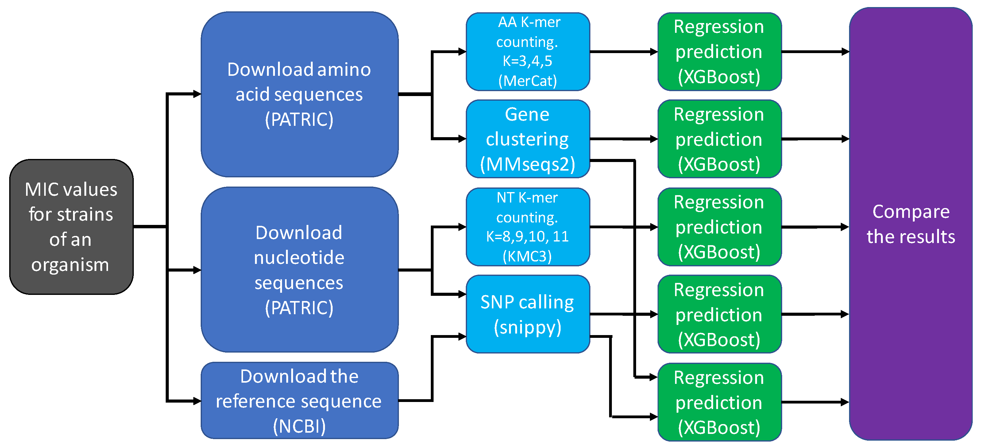
2. Methods
2.1. Data Acquisition and Pre-Processing
2.2. Feature Extraction Methods
2.2.1. Nucleotide k-mers
2.2.2. Amino Acid k-mers
2.2.3. Gene Content
2.2.4. SNP Calling
2.2.5. Gene Content and SNP Calling
2.3. Feature Matrix and Target Values
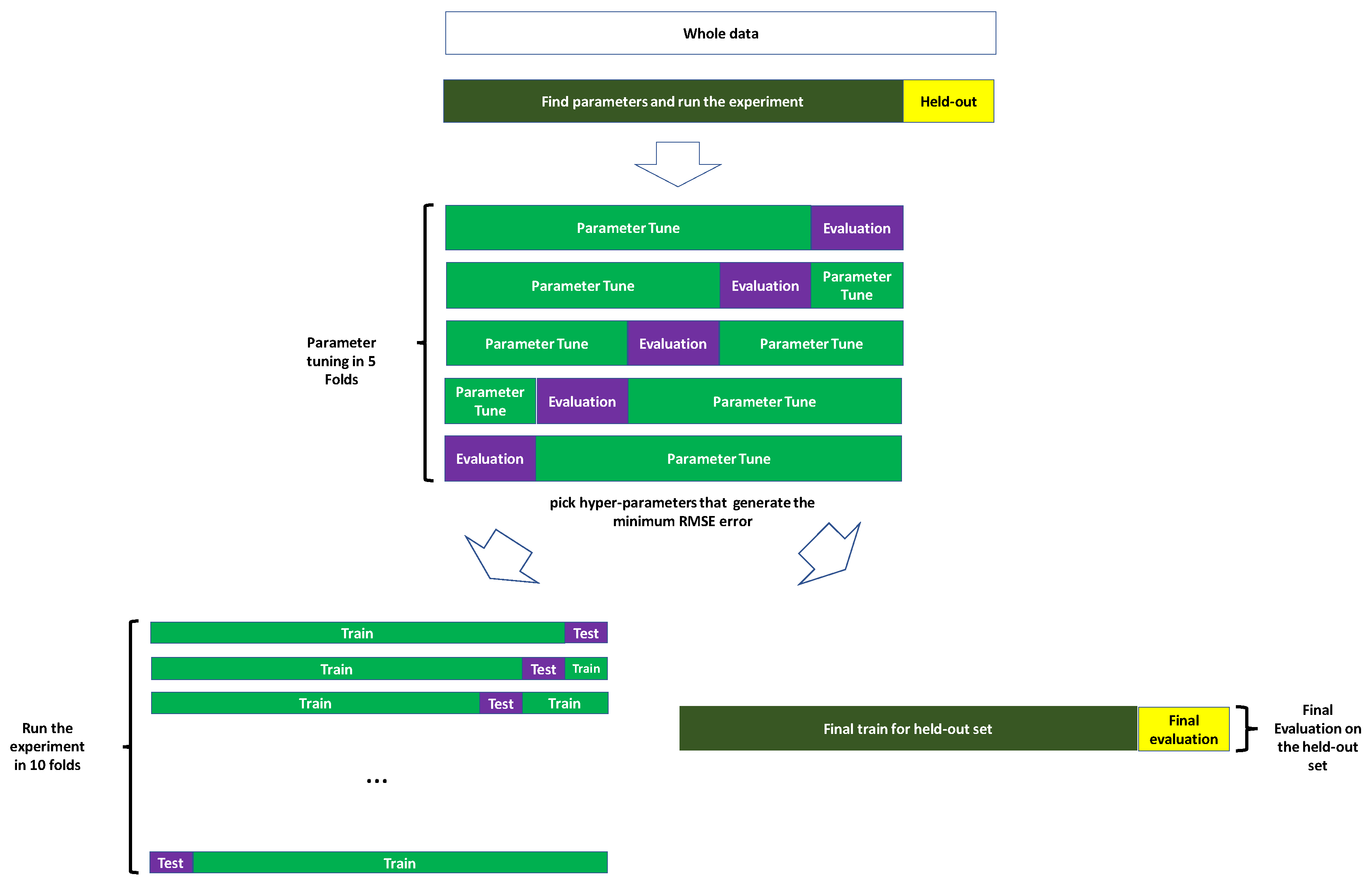
2.4. Measuring the Prediction Performance
2.5. Machine Learning
2.5.1. Hyper-Parameter Tuning For XGBoost
2.5.2. Training the Model
2.5.3. Feature Selection
- A concise model using only important features can be built.
- The features can be used to gain biological insights.
2.5.3.1. Feature Selection Pipeline
| Algorithm 1 Feature selection. |
|
2.5.3.2. Training the Model with the Selected Features
2.5.3.3. Tuning the Hyper-Parameter
2.5.3.4. Interpreting the Top Features
- Validation: When the model finds top features that we already know are important AMR determinants, we know that the model has been trained and is working properly.
- Discovery of new AMR determinants: In an accurate model, the top features that are derived from the data can be used for discovering new AMR genes/SNPs.
2.6. Software Implementation and Availability
3. Results
3.1. Performances of Different Feature Extraction Methods
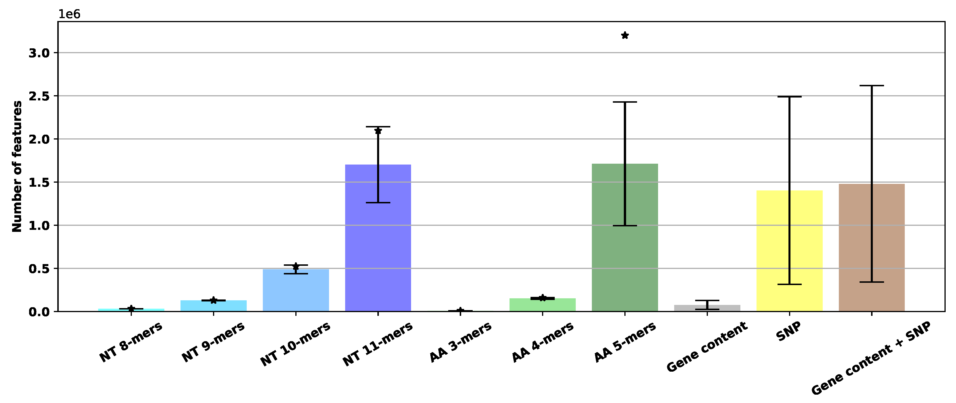
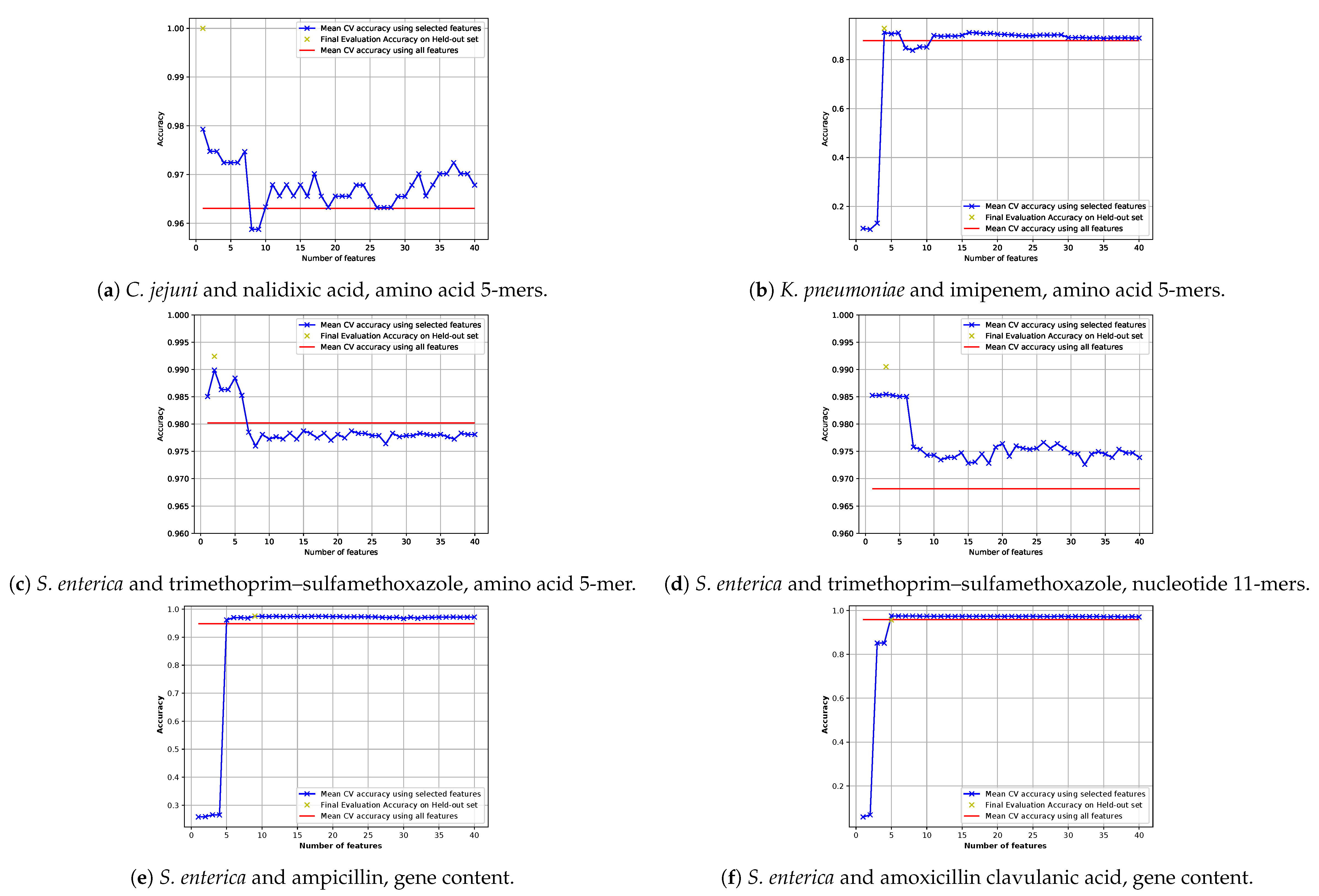
3.1.1. Comparison of Required Numbers of Features
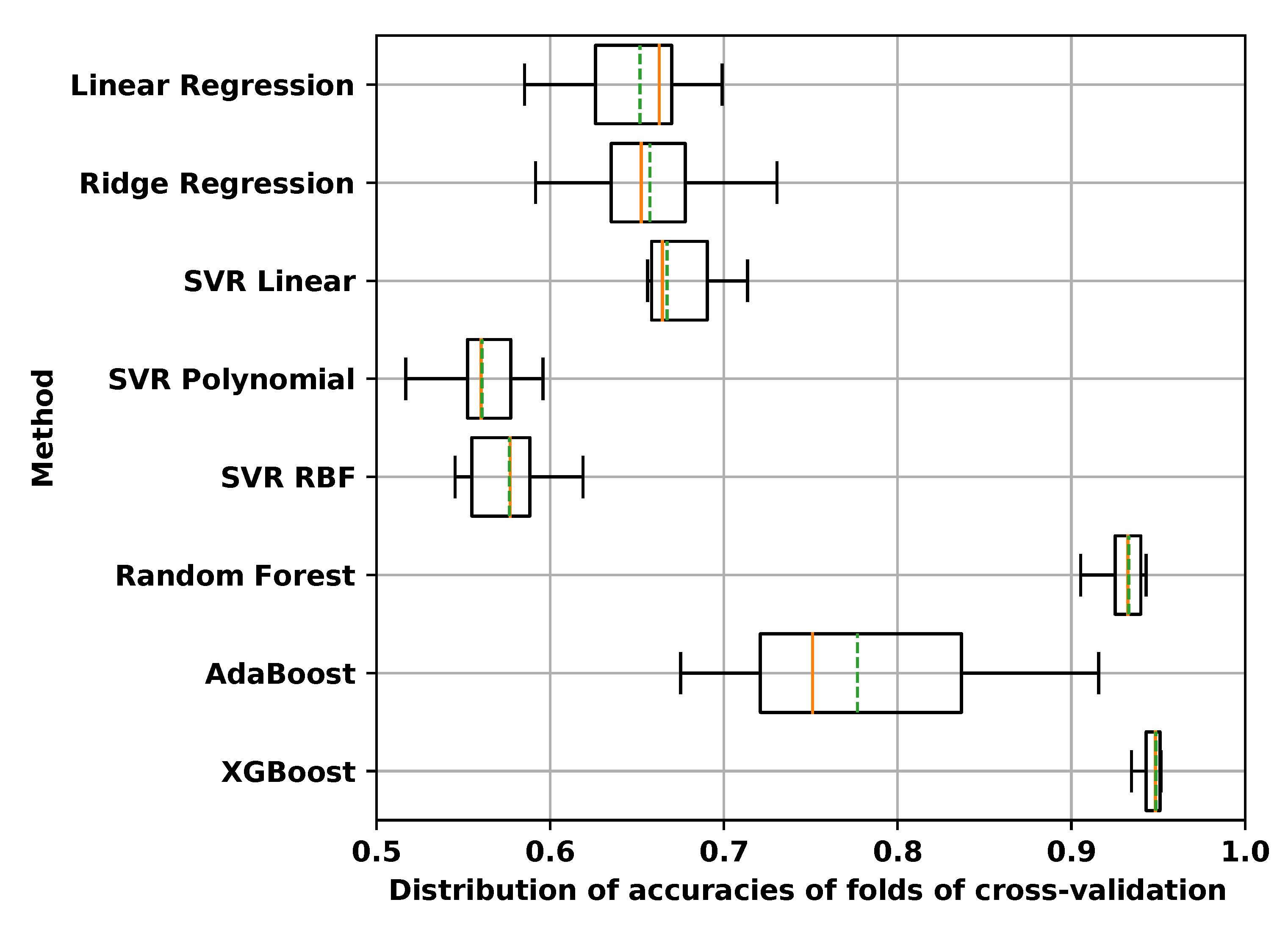
3.1.2. Comparison of Regression Packages
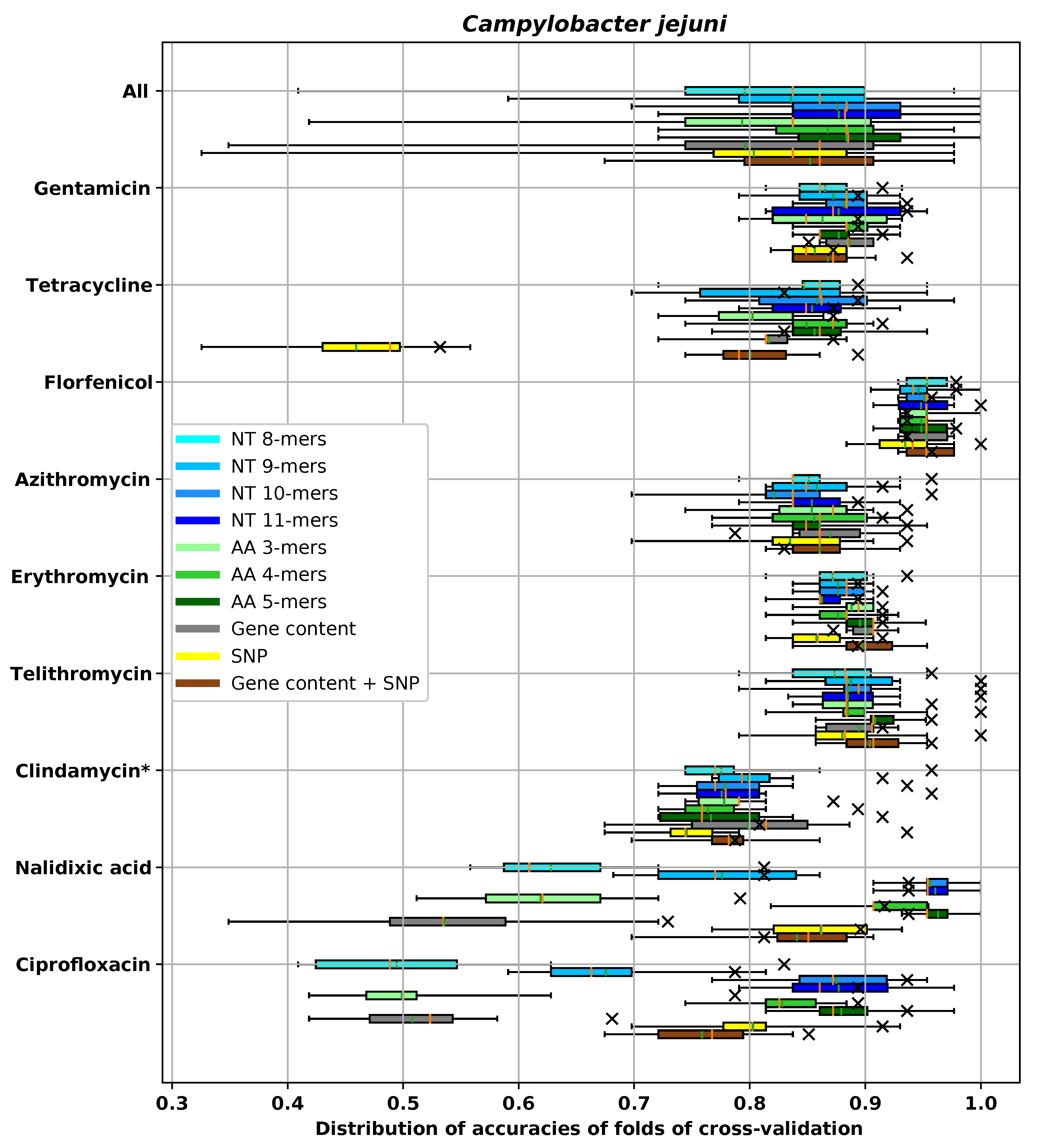
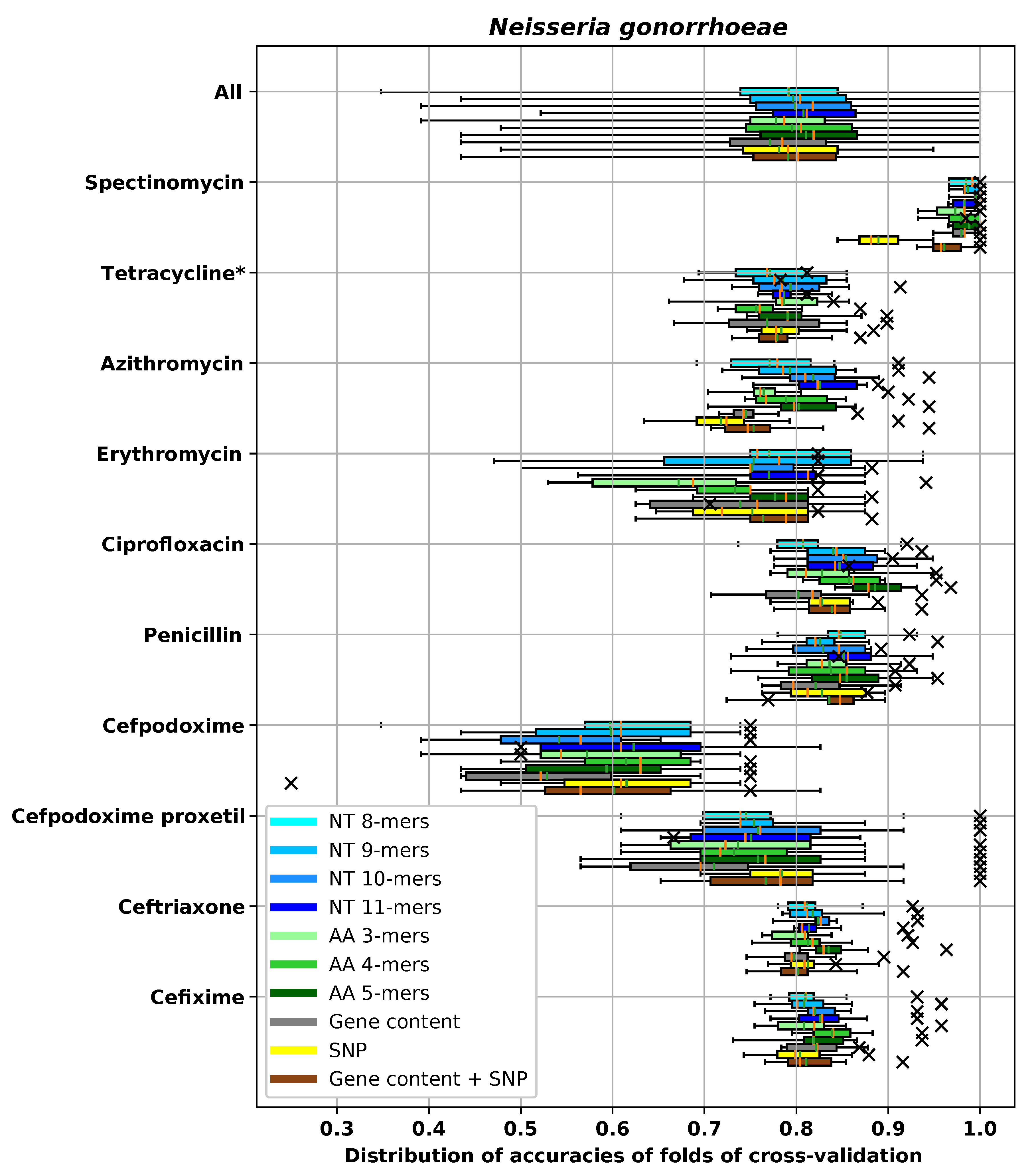
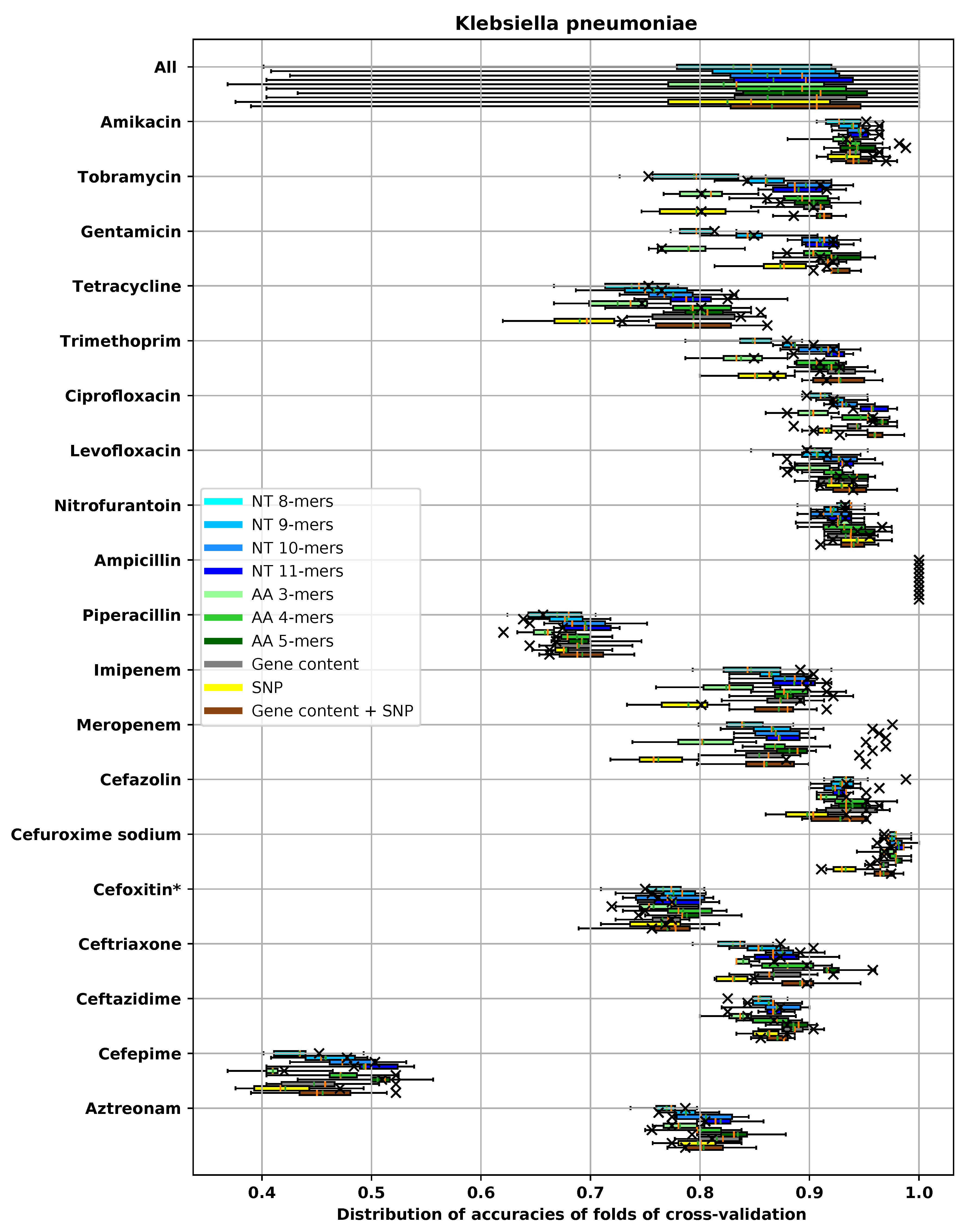
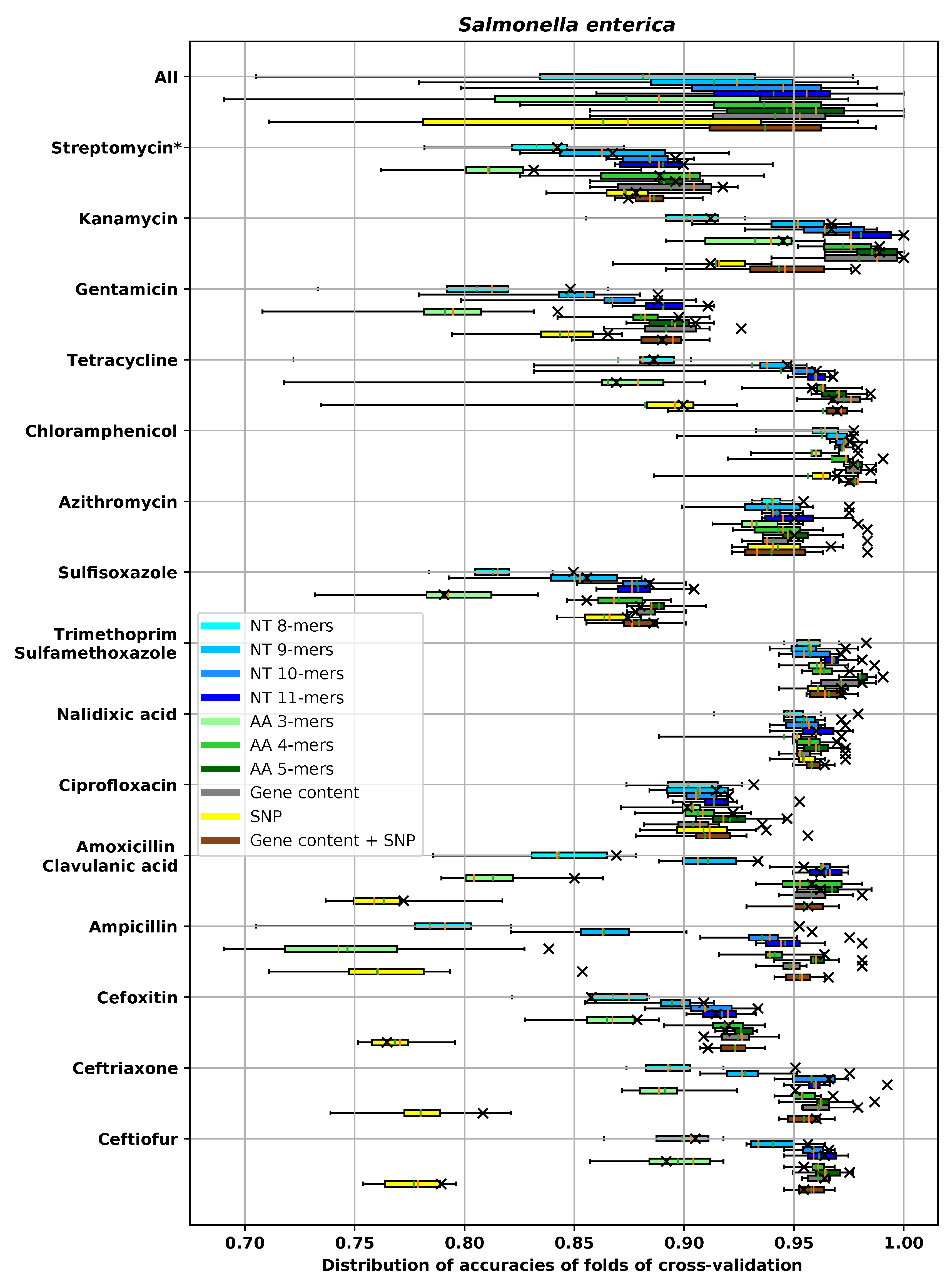
3.1.3. Accuracy of Different Feature Extraction Methods Using XGBoost
3.1.4. Searching Top Amino Acid and Nucleotide k-mers in NCBI Database
3.2. Analysis of AMR Determinants for Specific Antibiotics Families
3.2.1. Resistance to Tetracycline
Two Types of the tet(D) Gene
3.2.2. Resistance to Quinolone Antibiotics
3.2.3. Resistance to Aminoglycoside Antibiotics
3.2.4. Resistance to β-Lactam Antibiotics
Carbapenem Antibiotics
Cephalosporin Antibiotics
Other β-Lactam Antibiotics
3.2.5. Resistance to Chloramphenicol
3.2.6. Resistance to Sulfonamide
3.2.7. Resistance to Macrolide Antibiotics
4. Discussion
4.1. Requirement of Gene Assembly
4.2. Predicting AMr Accurately
4.3. Comparison of Required Number of Features
4.4. Interpretability of the Model
- Validation: mechanisms predicted to be important in an interpretable model can be compared to previously known AMR mechanisms, so that we know the model is working properly.
- Discovery: predictions of an interpretable model can be used to discover new AMR mechanisms that have not been discovered before.
5. Conclusions
Supplementary Materials
Author Contributions
Funding
Acknowledgments
Conflicts of Interest
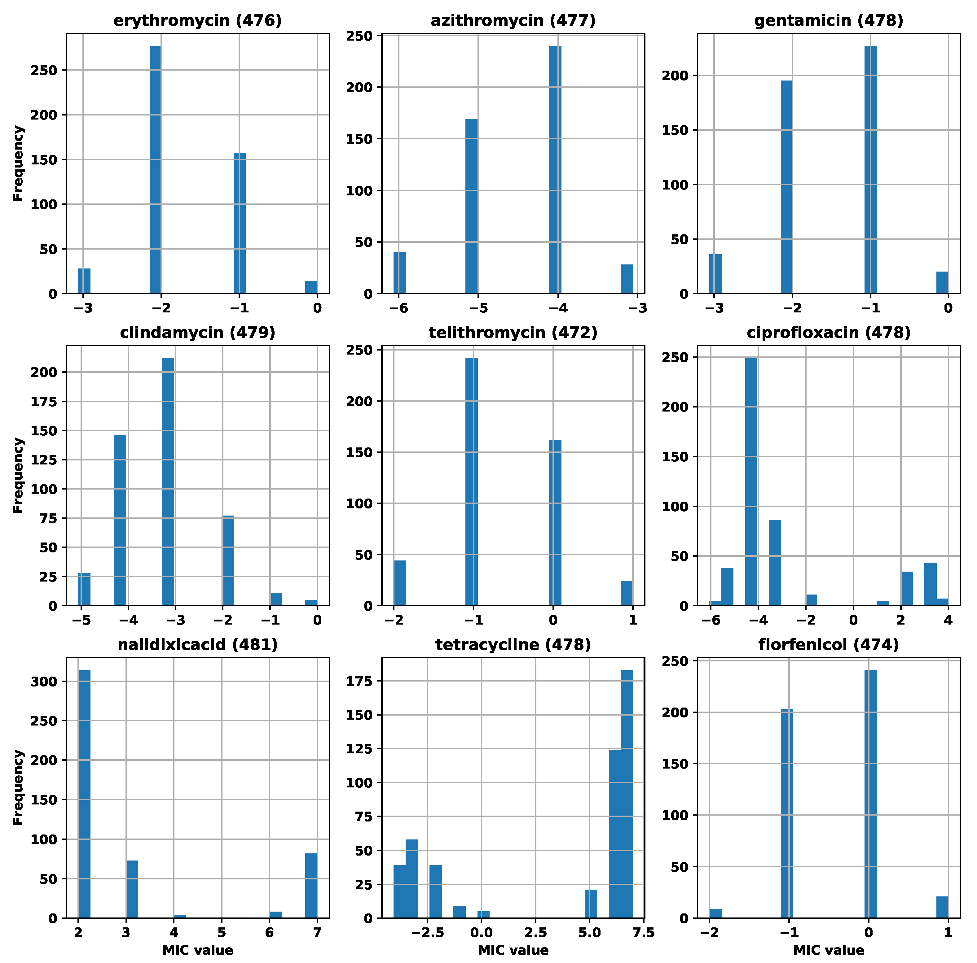
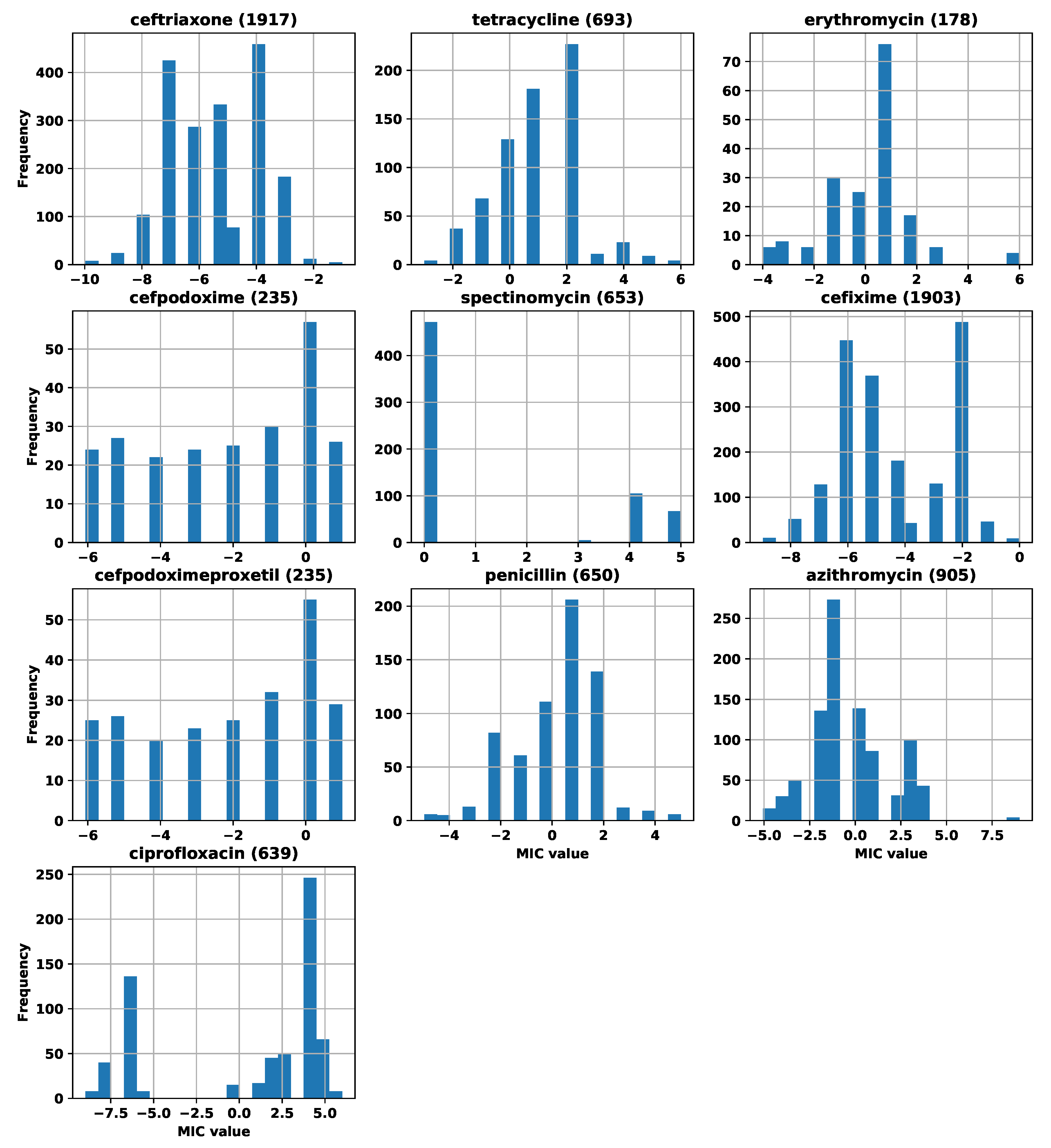
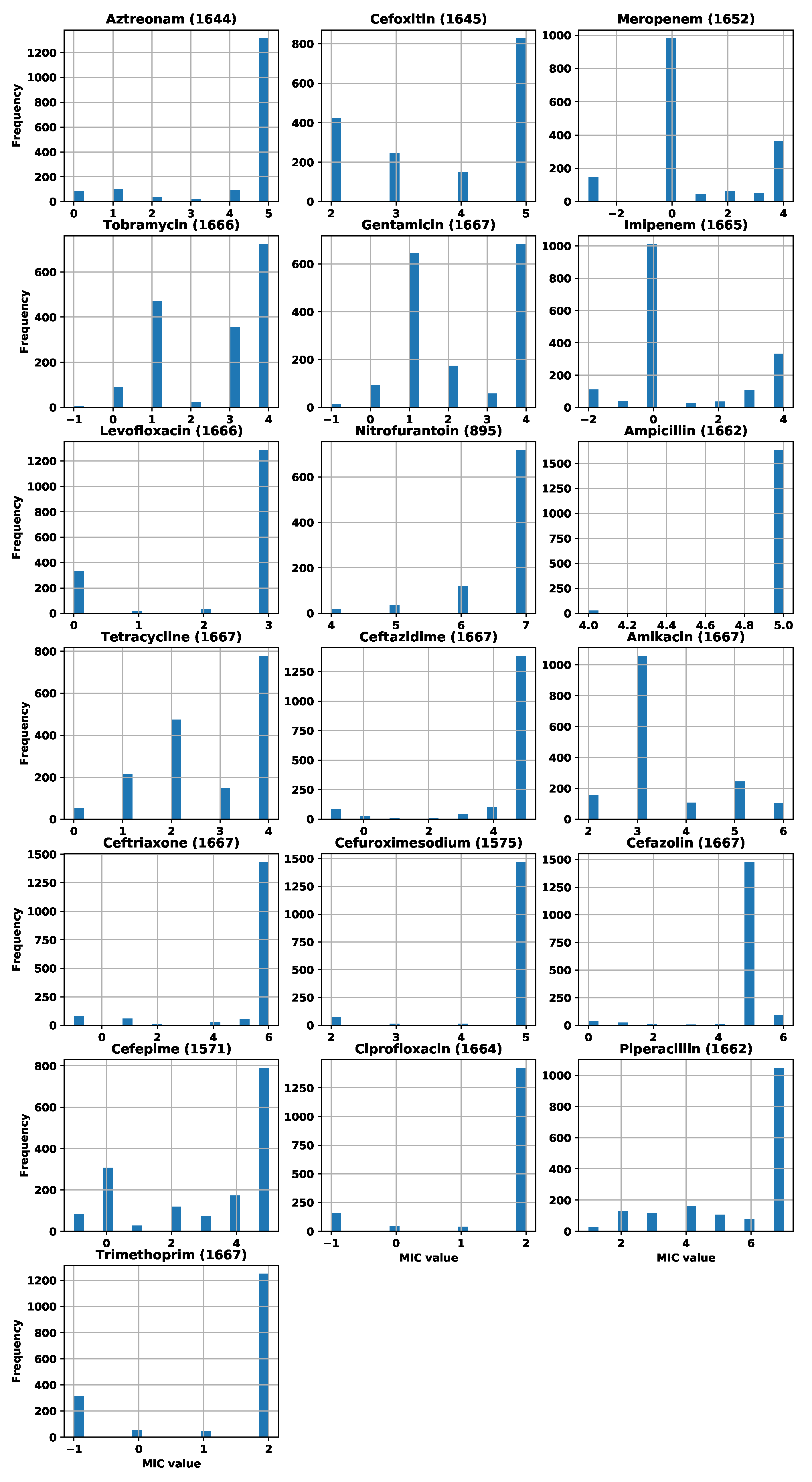
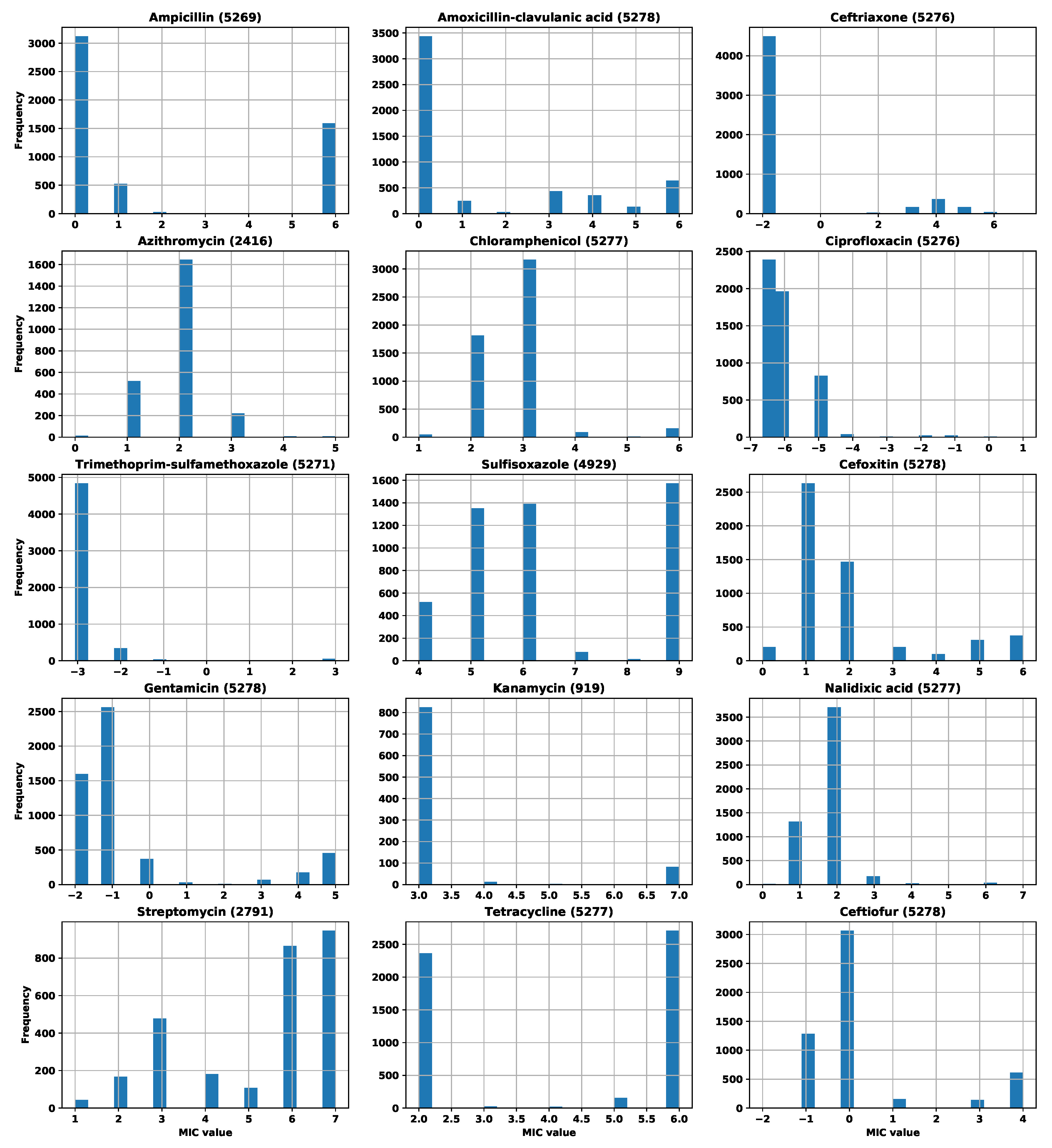
Appendix A. Number of Strains and MIC Distributions

| Antibiotic | Initial Number of Strains | Number of Strains after Filtering |
|---|---|---|
| erythromycin | 481 | 476 |
| azithromycin | 481 | 477 |
| gentamicin | 481 | 478 |
| clindamycin | 481 | 479 |
| telithromycin | 481 | 472 |
| ciprofloxacin | 481 | 478 |
| nalidixic acid | 481 | 481 |
| tetracycline | 481 | 478 |
| florfenicol | 481 | 474 |
| Antibiotic | Initial Number of Strains | Number of Strains after Filtering |
|---|---|---|
| ceftriaxone | 1926 | 1917 |
| tetracycline | 696 | 693 |
| erythromycin | 179 | 178 |
| cefpodoxime | 236 | 235 |
| spectinomycin | 655 | 653 |
| cefixime | 1907 | 1903 |
| cefpodoximeproxetil | 236 | 235 |
| penicillin | 655 | 650 |
| azithromycin | 911 | 905 |
| ciprofloxacin | 655 | 639 |
| Antibiotic | Initial Number of Strains | Number of Strains after Filtering |
|---|---|---|
| Aztreonam | 1644 | 1644 |
| Cefoxitin | 1645 | 1645 |
| Meropenem | 1660 | 1652 |
| Tobramycin | 1666 | 1666 |
| Gentamicin | 1667 | 1667 |
| Imipenem | 1666 | 1665 |
| Levofloxacin | 1666 | 1666 |
| Nitrofurantoin | 895 | 895 |
| Ampicillin | 1666 | 1662 |
| Tetracycline | 1667 | 1667 |
| Ceftazidime | 1667 | 1667 |
| Amikacin | 1667 | 1667 |
| Ceftriaxone | 1667 | 1667 |
| Cefuroximesodium | 1575 | 1575 |
| Cefazolin | 1667 | 1667 |
| Cefepime | 1571 | 1571 |
| Ciprofloxacin | 1664 | 1664 |
| Piperacillin | 1662 | 1662 |
| Trimethoprim | 1667 | 1667 |
| Antibiotic | Initial Number of Strains | Number of Strains after Filtering |
|---|---|---|
| Ampicillin | 5277 | 5269 |
| Amoxicillin-clavulanic acid | 5278 | 5278 |
| Ceftriaxone | 5278 | 5276 |
| Azithromycin | 2416 | 2416 |
| Chloramphenicol | 5277 | 5277 |
| Ciprofloxacin | 5277 | 5276 |
| Trimethoprim-sulfamethoxazole | 5277 | 5271 |
| Sulfisoxazole | 4929 | 4929 |
| Cefoxitin | 5278 | 5278 |
| Gentamicin | 5278 | 5278 |
| Kanamycin | 924 | 919 |
| Nalidixic acid | 5278 | 5277 |
| Streptomycin | 2791 | 2791 |
| Tetracycline | 5277 | 5277 |
| Ceftiofur | 5278 | 5278 |


Appendix B. Comparison of Number of Features for Nucleotide and Amino Acid k-mers
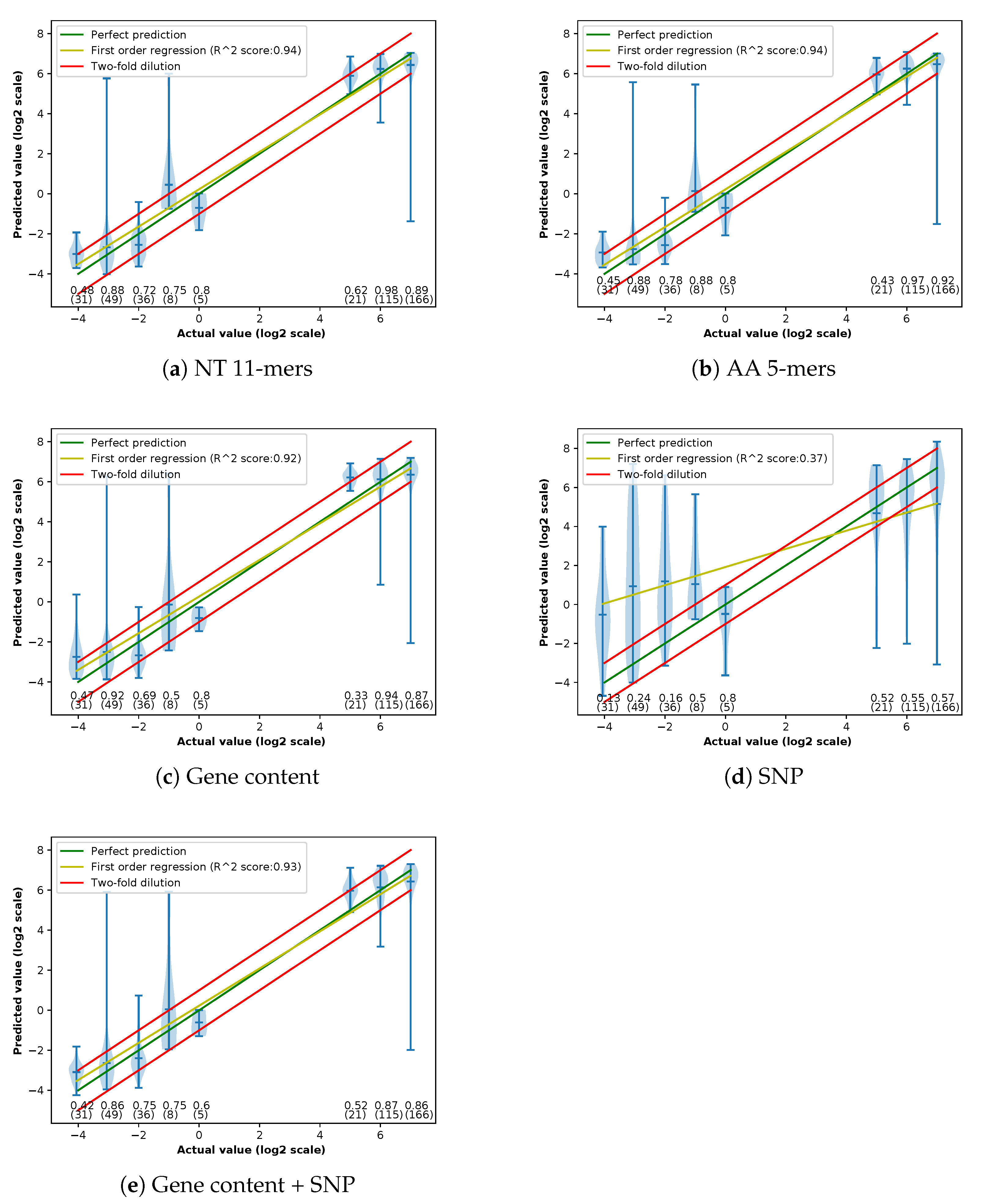
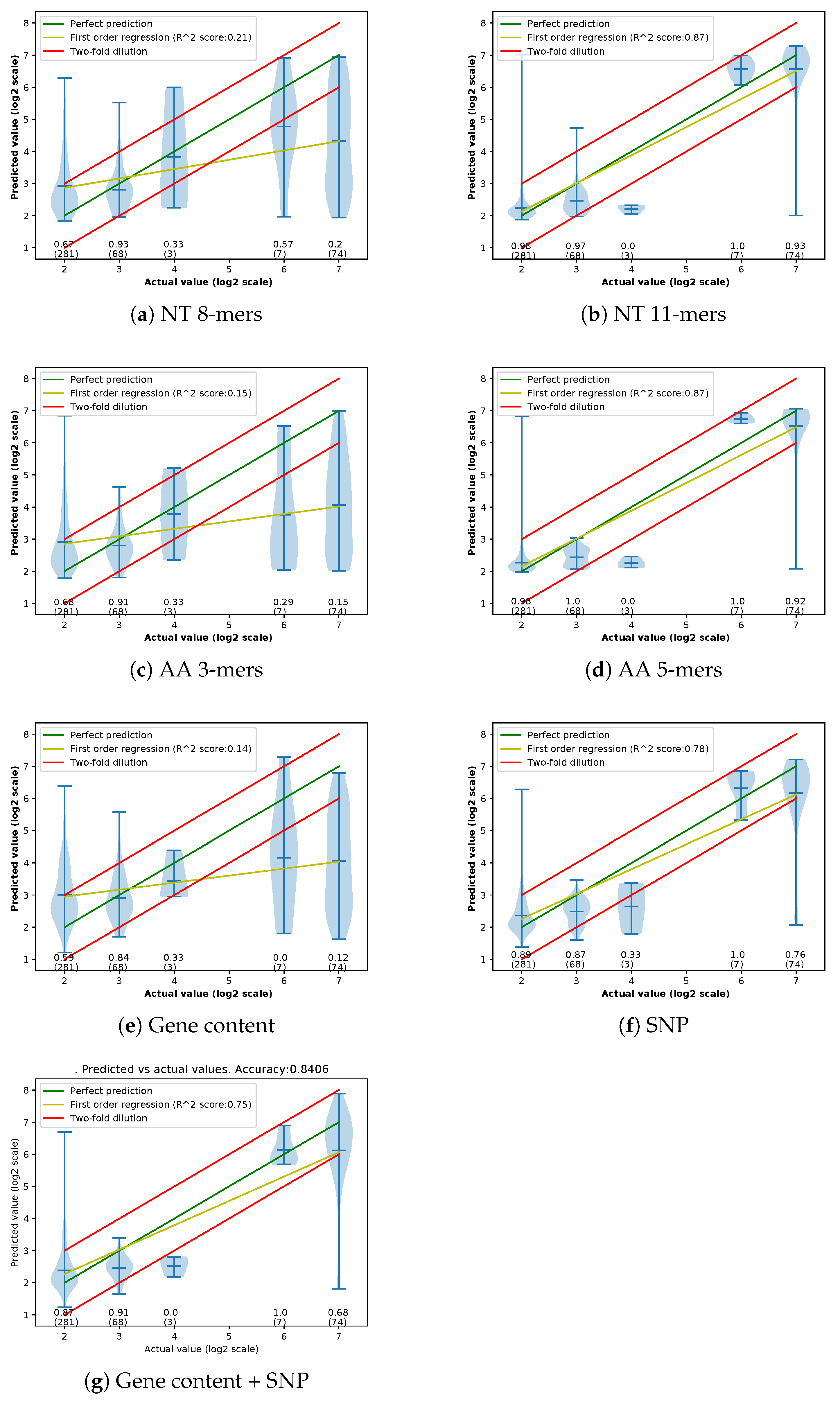
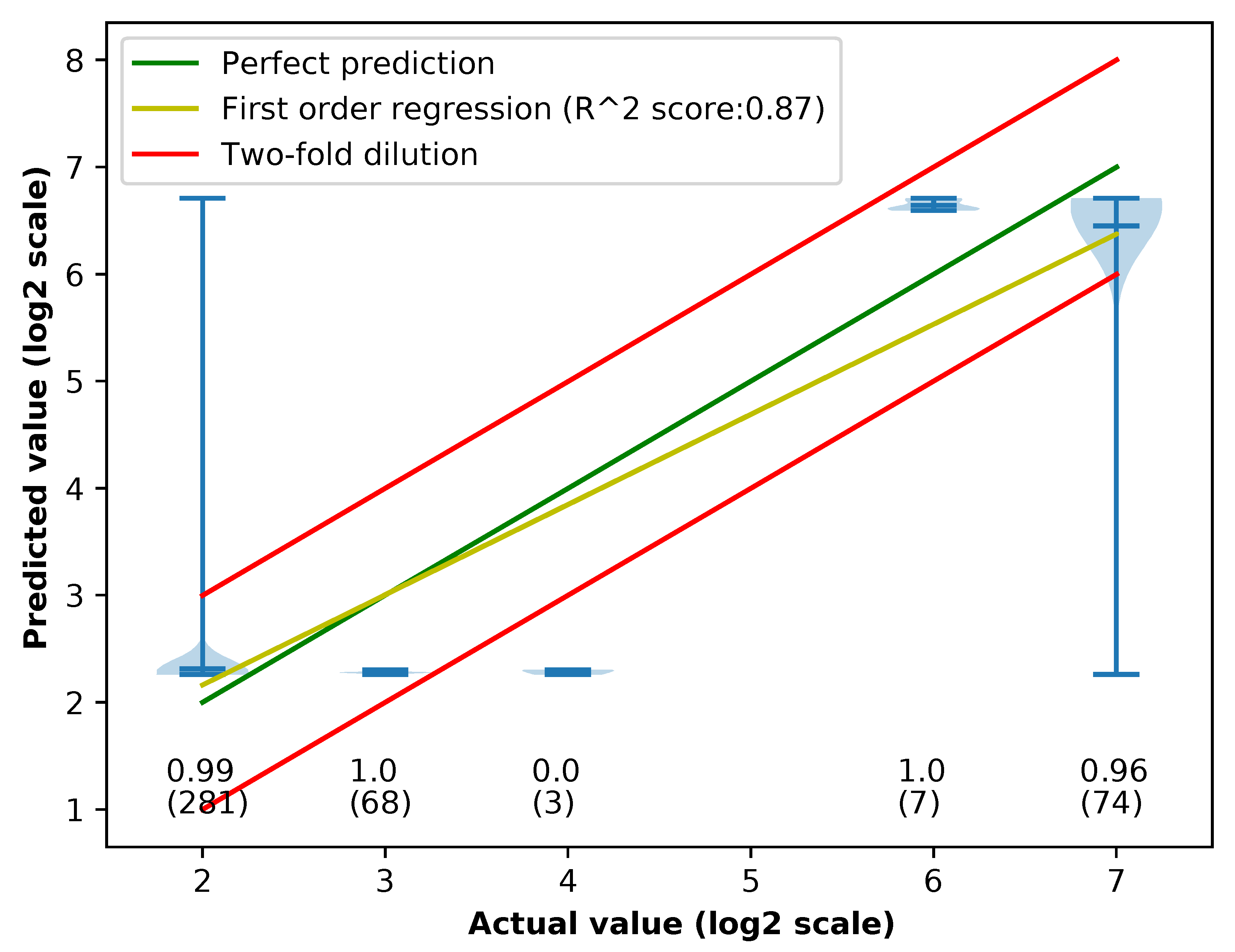
Appendix C. Violin Plots of Error in Different Methods


Appendix D. Important Features Found by the Models
| Amino Acid 5-mers | Gene Content | |||||||
|---|---|---|---|---|---|---|---|---|
| 5-mer | Gene Product | Number of +/− Strains | Mean (STD) MIC of +/− Strains | p-Value | Gene Product | Number of +/− Strains | Mean (STD) MIC of +/− Strains | p-Value |
| DGLTT | tetracycline resistance transcriptional repressor TetR | 635/1032 | 15.0 (3.3)/6.3 (5.1) | Permease of the drug/metabolite transporter (DMT) superfamily | 341/1326 | 15.8 (1.6)/8.0 (5.9) | ||
| HYGIL | tetracycline efflux MFS transporter Tet(A) | 642/1025 | 15.0 (3.3)/6.2 (5.0) | Tetracycline resistance regulatory protein TetR | 282/1385 | 14.5 (4.0)/8.6 (6.0) | ||
| IQWLI | undecaprenyl- phosphate galactose phosphotransferase WbaP | 113/1554 | 12.1 (5.7)/9.4 (6.2) | hypothetical protein (fig573.12878.peg.5387) | 115/1552 | 7.0 (6.8)/9.8 (6.1) | ||
| LRHCC | 41/1626 | 5.2 (4.3)/9.7 (6.2) | Tetracycline resistance, MFS efflux pump => Tet(D) | 73/1594 | 5.9 (4.6)/9.8 (6.2) | |||
| Tetracycline resistance regulatory protein TetR | 367/1300 | 15.8 (1.6)/7.9 (5.8) | ||||||
| Tetracycline resistance, MFS efflux pump => Tet(A) | 366/1301 | 15.8 (1.6)/7.9 (5.8) | ||||||
| Tetracycline resistance, MFS efflux pump => Tet(D) | 250/1417 | 15.7 (1.8)/8.5 (6.0) | ||||||
| Class A beta-lactamase (EC 3.5.2.6) => CTX-M family, extended-spectrum | 1003/664 | 11.3 (5.9)/7.0 (5.6) | ||||||
| hypothetical protein (fig573.12921.peg.5397) | 14/1653 | 2.4 (3.8)/9.7 (6.1) | ||||||
| Putative aminotransferase | 11/1656 | 5.9 (6.5)/9.6 (6.2) | 0.0061 | |||||
| FIG002577: Putative lipoprotein precursor | 205/1462 | 13.8 (4.3)/9.0 (6.2) | ||||||
| hypothetical protein (fig573.12941.peg.329) | 18/1649 | 4.2 (5.3)/9.7 (6.1) | ||||||
| Amino Acid 5-mers | Gene Content | |||||||
|---|---|---|---|---|---|---|---|---|
| 5-mer | Gene Product | Number of +/− Strains | Mean (STD) MIC of +/− Strains | p-Value | Gene Product | Number of +/− Strains | Mean (STD) MIC of +/− Strains | p-Value |
| PYEET | aminoglycoside N-acetyltransferase AAC(3)-IIe | 627/1039 | 9.8 (5.7)/9.0 (6.5) | 0.0016 | Mobile element protein | 324/1342 | 15.6 (2.0)/7.8 (6.0) | |
| QFLRK | OXA-1 family class D beta-lactamase | 764/902 | 14.2 (3.7)/5.2 (4.9) | Class D beta-lactamase (EC 3.5.2.6) => OXA-1 family | 379/1287 | 13.4 (3.9)/8.1 (6.3) | ||
| GSEMC | 160/1506 | 6.2 (6.5)/9.7 (6.1) | Chloramphenicol O-acetyltransferase (EC 2.3.1.28) => CatB family | 354/1312 | 13.3 (3.9)/8.3 (6.4) | |||
| DASMV | aminoglycoside N-acetyltransferase AAC(3)-IIe | 1476/190 | 9.7 (6.3)/6.5 (4.9) | Aminoglycoside N(6’)-acetyltransferase (EC 2.3.1.82) => AAC(6’)-Ib/AAC(6’)-II | 681/985 | 14.0 (3.7)/6.1 (5.6) | ||
| Mobile element protein | 58/1608 | 12.0 (5.9)/9.2 (6.3) | 0.0015 | |||||
| hypothetical protein (fig573.14286.peg.4244) | 379/1287 | 7.3 (5.2)/9.9 (6.4) | ||||||
| hypothetical protein (fig573.14233.peg.3013) | 431/1235 | 15.2 (3.0)/7.3 (5.8) | ||||||
| Aminoglycoside 3”-nucleotidyltransferase (EC 2.7.7.-) => ANT(3”)-Ia (AadA family) | 84/1582 | 13.9 (4.7)/9.1 (6.2) | ||||||
| hypothetical protein (fig573.12921.peg.5397) | 14/1652 | 2.1 (3.9)/9.4 (6.2) | ||||||
| hypothetical protein (fig573.14286.peg.510) | 619/1047 | 5.9 (5.1)/11.3 (6.0) | ||||||
| hypothetical protein (fig573.13822.peg.6818) | 17/1649 | 5.8 (5.3)/9.4 (6.3) | 0.025 | |||||
| Mobile element protein | 38/1628 | 5.9 (4.5)/9.4 (6.3) | 0.00096 | |||||
| hypothetical protein (fig573.12887.peg.5713) | 220/1446 | 14.2 (3.7)/8.6 (6.2) | ||||||
| Amino Acid 5-mers | Gene Content | |||||||
|---|---|---|---|---|---|---|---|---|
| 5-mer | Gene Product | Number of +/− Strains | Mean (STD) MIC of +/− Strains | p-Value | Gene Product | Number of +/− Strains | Mean (STD) MIC of +/− Strains | p-Value |
| SEPTR | 169/1497 | 1.8 (4.4)/4.8 (6.1) | 1.2e-76 | Heat shock protein 60 kDa family chaperone GroEL | 11/1655 | 16.0 (0.0)/4.4 (6.0) | ||
| TCGVY | carbapenem- hydrolyzing class A beta-lactamase KPC | 487/1179 | 12.2 (5.3)/1.3 (2.1) | hypothetical protein (fig573.12981.peg.5967) | 31/1635 | 3.1 (5.8)/4.5 (6.0) | ||
| CIRDR | 162/1504 | 1.6 (4.0)/4.8 (6.1) | Anaerobic dimethyl sulfoxide reductase chain B (EC 1.8.5.3), iron-sulfur binding subunit | 261/1405 | 2.4 (4.7)/4.8 (6.2) | |||
| GWIKI | 16S rRNA (guanine(1405)- N(7))- methyltransferase | 15/1651 | 13.1 (5.1)/4.4 (6.0) | hypothetical protein (fig573.14374.peg.5559) | 11/1655 | 14.9 (3.4)/4.4 (6.0) | ||
| LDFPD | BNR-4 repeat-containing protein | 16/1650 | 12.1 (6.1)/4.4 (6.0) | 0.00011 | Periplasmic divalent cation tolerance protein CutA | 11/1655 | 16.0 (0.0)/4.4 (6.0) | |
| WELEL | KPC family carbapenem- hydrolyzing class A beta-lactamase | 491/1175 | 12.2 (5.4)/1.3 (2.1) | hypothetical protein (fig573.12878.peg.5387) | 115/1551 | 1.6 (4.1)/4.7 (6.1) | ||
| Transposase | 477/1189 | 12.3 (5.3)/1.3 (2.3) | ||||||
| Class A beta-lactamase (EC 3.5.2.6) => KPC family, carbapenem-hydrolyzing | 488/1178 | 12.2 (5.4)/1.3 (2.2) | ||||||
| Transposase InsH for insertion sequence element IS5 | 10/1656 | 0.2 (0.0)/4.5 (6.0) | ||||||
| Mobile element protein | 9/1657 | 1.4 (2.3)/4.5 (6.0) | 0.0074 | |||||
| hypothetical protein (fig573.13500.peg.3164) | 186/1480 | 1.3 (2.2)/4.9 (6.2) | ||||||
| hypothetical protein (fig573.14417.peg.5283) | 6/1660 | 11.0 (7.1)/4.4 (6.0) | 0.025 | |||||
| Mobile element protein | 479/1187 | 12.3 (5.3)/1.3 (2.2) | ||||||
| Mobile element protein | 56/1610 | 1.4 (2.1)/4.6 (6.1) | 0.036 | |||||
| IS, phage, Tn; Transposon-related functions | 10/1656 | 14.8 (3.6)/4.4 (6.0) | ||||||
| Amino Acid 5-mers | Gene Content | |||||||
|---|---|---|---|---|---|---|---|---|
| 5-mer | Gene Product | Number of +/− Strains | Mean (STD) MIC of +/− Strains | p-Value | Gene Product | Number of +/− Strains | Mean (STD) MIC of +/− Strains | p-Value |
| ANKSY | CMY-2 family class C beta-lactamase | 714/4458 | 46.0 (18.7)/3.1 (3.3) | 0.0 | Outer membrane porin OmpD | 4172/1106 | 8.8 (16.5)/10.3 (17.4) | |
| TWITV | CMY-2 family class C beta-lactamase | 713/4459 | 45.9 (18.7)/3.1 (3.4) | 0.0 | Mobile element protein | 840/4438 | 38.2 (23.2)/3.6 (6.2) | 0.0 |
| GNTHP | 9/5163 | 11.6 (18.7)/9.0 (16.6) | 0.048 | Class C beta-lactamase (EC 3.5.2.6) => CMY/CMY-2/CFE/LAT family | 736/4542 | 45.7 (18.7)/3.2 (3.7) | 0.0 | |
| VRTFP | 110/5062 | 4.4 (7.8)/9.1 (16.7) | 0.00044 | Putative outer membrane lipoprotein | 6/5272 | 16.0 (0.0)/9.1 (16.7) | 0.00088 | |
| QNTRI | 12/5160 | 20.3 (23.0)/9.0 (16.6) | 0.049 | Small multidrug resistance (SMR) efflux transporter => SugE, quaternary ammonium compounds | 696/4582 | 46.0 (18.6)/3.5 (5.4) | 0.0 | |
| HTWIT | CMY-2 family class C beta-lactamase | 713/4459 | 45.9 (18.7)/3.1 (3.4) | 0.0 | FIG01046993: hypothetical protein | 440/4838 | 42.5 (23.5)/6.1 (12.0) | |
| Cobalamin synthase (EC 2.7.8.26) | 5/5273 | 33.6 (26.8)/9.1 (16.7) | 0.0048 | |||||
| Amino Acid 5-mers | Gene Content | |||||||
|---|---|---|---|---|---|---|---|---|
| 5-mer | Gene Product | Number of +/− Strains | Mean (STD) MIC of +/− Strains | p-Value | Gene Product | Number of +/− Strains | Mean (STD) MIC of +/− Strains | p-Value |
| WMRDD | class A beta-lactamase | 56/5221 | 62.9 (8.3)/19.7 (28.6) | Class A beta-lactamase (EC 3.5.2.6) => TEM family | 815/4462 | 63.2 (7.1)/12.3 (23.9) | 0.0 | |
| TDFLR | class A beta-lactamase | 143/5134 | 45.5 (28.7)/19.4 (28.5) | Class A beta-lactamase (EC 3.5.2.6) => HER family | 56/5221 | 62.9 (8.3)/19.7 (28.6) | ||
| ASWVH | CMY-2 family class C beta-lactamase | 745/4532 | 62.9 (8.1)/13.1 (24.6) | 0.0 | Mobile element protein | 294/4983 | 63.8 (3.7)/17.6 (27.6) | |
| AMSQN | response regulator transcription factor | 10/5267 | 45.4 (28.4)/20.1 (28.8) | 0.0051 | hypothetical protein (fig590.14012.peg.5176) | 106/5171 | 63.4 (6.0)/19.2 (28.4) | |
| TMSDN | TEM family class A beta-lactamase | 1091/4186 | 57.2 (19.5)/10.5 (22.3) | 0.0 | Class A beta-lactamase (EC 3.5.2.6) => CARB/PSE family, carbenicillin-hydrolyzing | 42/5235 | 61.1 (13.1)/19.8 (28.7) | |
| RDIGY | 26/5251 | 49.6 (26.3)/20.0 (28.8) | Integrase | 5/5272 | 64.0 (0.0)/20.1 (28.8) | 0.002 | ||
| NTAAN | type IV conjugative transfer system coupling protein TraD | 868/4409 | 62.9 (8.3)/11.7 (23.5) | 0.0 | DNA replication protein | 26/5251 | 49.6 (26.3)/20.0 (28.8) | |
| VIYQG | CMY-2 family class C beta-lactamase | 751/4526 | 62.5 (9.5)/13.1 (24.6) | 0.0 | Class C beta-lactamase (EC 3.5.2.6) => CMY/CMY-2/CFE/LAT family | 736/4541 | 63.1 (7.5)/13.2 (24.7) | 0.0 |
| YWDYN | TolC family protein | 42/5235 | 61.1 (13.1)/19.8 (28.7) | ABC transporter involved in cytochrome c biogenesis, ATPase component CcmA | 4/5273 | 64.0 (0.0)/20.1 (28.8) | 0.0056 | |
| hypothetical protein (fig590.17530.peg.3704) | 4/5273 | 64.0 (0.0)/20.1 (28.8) | 0.0056 | |||||
| Amino Acid 5-mers | Gene Content | |||||||
|---|---|---|---|---|---|---|---|---|
| 5-mer | Gene Product | Number of +/− Strains | Mean (STD) MIC of +/− Strains | p-Value | Gene Product | Number of +/− Strains | Mean (STD) MIC of +/− Strains | p-Value |
| WAYTL | chloramphenicol/florfenicol efflux MFS transporter FloR | 146/5131 | 63.3 (6.1)/6.8 (3.7) | Chloramphenicol resistance, MFS efflux pump => CmlA family | 26/5251 | 56.0 (14.9)/8.2 (9.4) | ||
| TAWPV | CmlA family chloramphenicol efflux MFS transporter | 169/5108 | 57.7 (17.3)/6.8 (3.3) | Chloramphenicol/florfenicol resistance, MFS efflux pump => FloR family | 146/5131 | 63.3 (6.1)/6.8 (3.7) | ||
| CDGFH | type A chloramphenicol O-acetyltransferase | 6/5271 | 64.0 (0.0)/8.3 (9.8) | hypothetical protein (fig590.14843.peg.2228) | 4061/1216 | 9.4 (10.9)/5.2 (4.9) | ||
| QGSGN | Select seq gbEAX8474651.1 RHS repeat protein | 1308/3969 | 6.4 (9.9)/9.0 (10.0) | Small multidrug resistance (SMR) efflux transporter => QacE, quaternary ammonium compounds | 13/5264 | 47.4 (18.9)/8.3 (9.8) | ||
| YMVML | chloramphenicol/florfenicol efflux MFS transporter FloR | 146/5131 | 63.3 (6.1)/6.8 (3.7) | Transposase, IS3/IS911 family | 692/4585 | 6.5 (5.8)/8.7 (10.5) | ||
| MDIYL | chloramphenicol/florfenicol efflux MFS transporter FloR | 146/5131 | 63.3 (6.1)/6.8 (3.7) | Glycosyltransferase | 1179/4098 | 6.6 (10.3)/8.9 (9.9) | ||
| FRMAM | amino acid adenylation domain-containing protein | 6/5271 | 64.0 (0.0)/8.3 (9.8) | Transcriptional regulator, LysR family | 107/5170 | 64.0 (0.0)/7.2 (6.1) | ||
| PVFTM | type A chloramphenicol O-acetyltransferase | 9/5268 | 45.8 (25.9)/8.3 (9.8) | Tetracycline resistance regulatory protein TetR | 38/5239 | 61.3 (11.6)/8.0 (8.9) | ||
| FAKFF | type IV secretion system protein TraC | 7/5270 | 17.1 (19.3)/8.4 (10.0) | 0.0094 | Inner membrane protein of type IV secretion of T-DNA complex, TonB-like, VirB10 | 6/5271 | 17.3 (20.9)/8.4 (10.0) | 0.041 |
| Cytochrome c-type heme lyase subunit nrfE, nitrite reductase complex assembly | 1960/3317 | 10.3 (13.4)/7.3 (7.1) | ||||||
| Type I secretion system ATPase, LssB family LapB | 41/5236 | 5.3 (2.0)/8.4 (10.0) | ||||||
| hypothetical protein (fig590.13820.peg.5180) | 48/5229 | 52.2 (22.0)/8.0 (8.9) | ||||||
| YbjA protein | 4/5273 | 64.0 (0.0)/8.4 (9.9) | ||||||
| Chloramphenicol O-acetyltransferase (EC 2.3.1.28) => CatA1/CatA4 family | 4/5273 | 64.0 (0.0)/8.4 (9.9) | ||||||
| Transcriptional regulator, LysR family | 2478/2799 | 8.3 (8.7)/8.5 (11.1) | ||||||
| Mobile element protein | 119/5158 | 59.9 (14.5)/7.2 (5.9) | ||||||
| Phosphomannomutase (EC 5.4.2.8) | 1180/4097 | 6.6 (10.3)/8.9 (9.9) | ||||||
| Mercuric transport protein, MerT | 450/4827 | 18.8 (22.3)/7.4 (7.2) | ||||||
| Amino Acid 5-mers | Gene Content | |||||||
|---|---|---|---|---|---|---|---|---|
| 5-mer | Gene Product | Number of +/− Strains | Mean (STD) MIC of +/− Strains | p-Value | Gene Product | Number of +/− Strains | Mean (STD) MIC of +/− Strains | p-Value |
| LDPGM | sulfonamide- resistant dihydropteroate synthase Sul1 | 1565/3364 | 501.2 (69.6)/52.1 (59.6) | 0.0 | Mobile element protein | 22/4907 | 512.0 (0.0)/193.3 (217.8) | |
| GMGFF | sulfonamide- resistant dihydropteroate synthase Sul1 | 1552/3377 | 505.0 (56.1)/52.1 (59.4) | 0.0 | Dihydropteroate synthase type-2 (EC 2.5.1.15) @ Sulfonamide resistance protein | 578/4351 | 506.7 (49.0)/153.3 (197.6) | |
| hypothetical protein (fig590.17526.peg.3772) | 802/4127 | 506.2 (51.5)/134.2 (184.1) | ||||||
| Aminoglycoside 3”-nucleotidyltransferase (EC 2.7.7.-) => ANT(3”)-Ia (AadA family) | 138/4791 | 508.8 (38.0)/185.7 (214.6) | ||||||
| Dihydropteroate synthase type-2 (EC 2.5.1.15) @ Sulfonamide resistance protein | 985/3944 | 506.4 (50.7)/116.9 (169.1) | 0.0 | |||||
| DNA recombination protein RmuC | 18/4911 | 512.0 (0.0)/193.6 (217.9) | ||||||
| Muconolactone isomerase (EC 5.3.3.4),putative | 818/4111 | 485.0 (108.4)/137.0 (186.3) | ||||||
Appendix E. Performance Evaluation
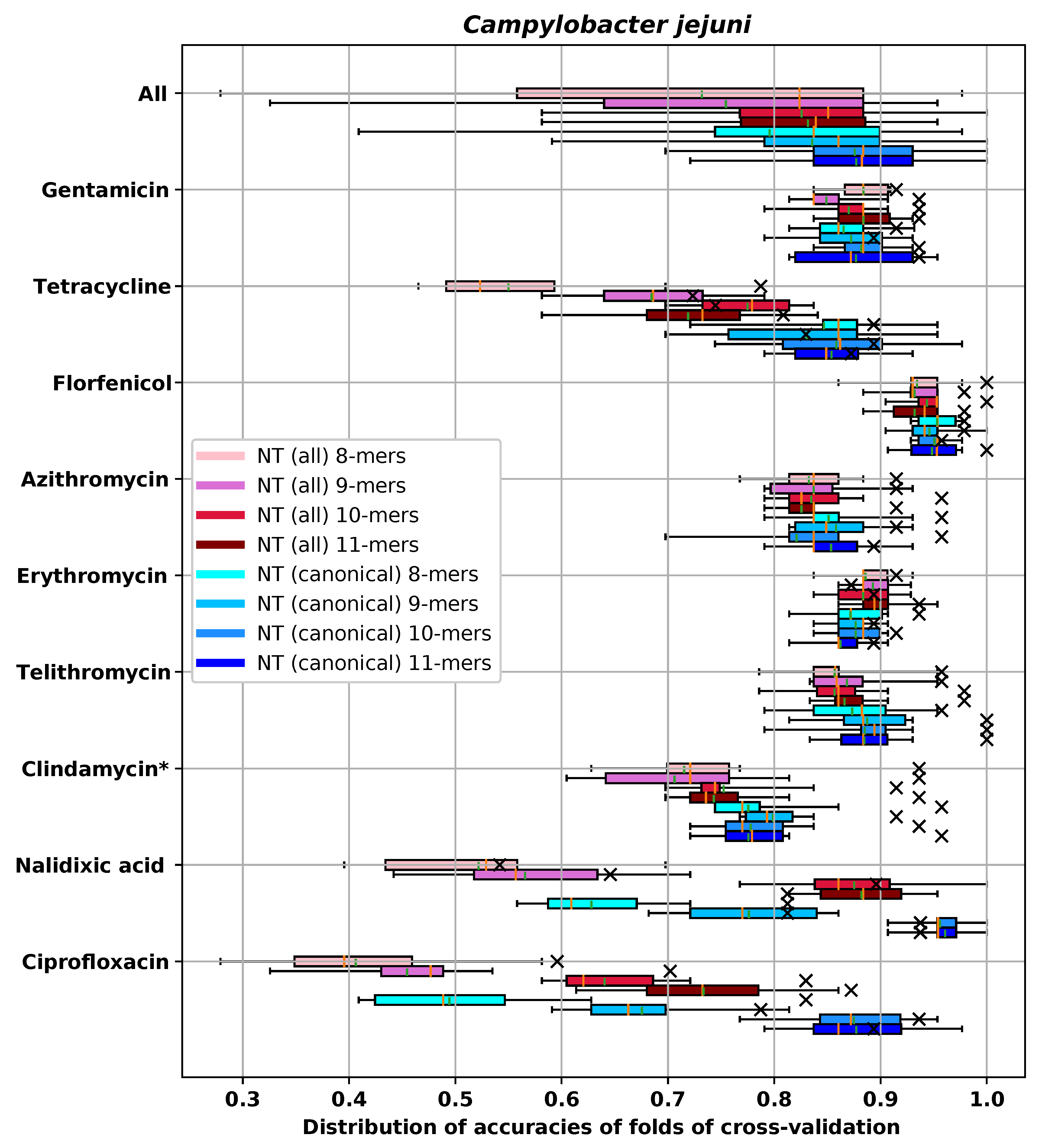
Appendix E.1. C. Jejuni
| RMSE-CV | RMSE-H | DD1-CV | DD1-H | DD2-CV | DD2-H | ME-CV | ME-H | VME-CV | VME-H | |
|---|---|---|---|---|---|---|---|---|---|---|
| NT 8-mers | 0.65 (0.027) | 0.457 | 0.872 (0.03) | 0.936 | 0.991 (0.011) | 1.000 | 0.0 (0.0) | 0.0 | 0.0 (0.0) | 0.0 |
| NT 9-mers | 0.626 (0.038) | 0.587 | 0.877 (0.021) | 0.894 | 0.995 (0.009) | 0.979 | 0.0 (0.0) | 0.0 | 0.0 (0.0) | 0.0 |
| NT 10-mers | 0.607 (0.038) | 0.554 | 0.877 (0.025) | 0.915 | 1.0 (0.0) | 1.000 | 0.0 (0.0) | 0.0 | 0.0 (0.0) | 0.0 |
| NT 11-mers | 0.622 (0.035) | 0.586 | 0.862 (0.025) | 0.894 | 0.998 (0.007) | 1.000 | 0.0 (0.0) | 0.0 | 0.0 (0.0) | 0.0 |
| AA 3-mers | 0.615 (0.03) | 0.553 | 0.888 (0.023) | 0.915 | 0.995 (0.009) | 1.000 | 0.0 (0.0) | 0.0 | 0.0 (0.0) | 0.0 |
| AA 4-mers | 0.604 (0.034) | 0.581 | 0.877 (0.029) | 0.915 | 0.998 (0.007) | 1.000 | 0.0 (0.0) | 0.0 | 0.0 (0.0) | 0.0 |
| AA 5-mers | 0.598 (0.042) | 0.566 | 0.895 (0.03) | 0.915 | 1.0 (0.0) | 1.000 | 0.0 (0.0) | 0.0 | 0.0 (0.0) | 0.0 |
| Gene content | 0.6 (0.041) | 0.605 | 0.902 (0.014) | 0.872 | 1.0 (0.0) | 1.000 | 0.0 (0.0) | 0.0 | 0.0 (0.0) | 0.0 |
| SNP | 0.624 (0.046) | 0.593 | 0.858 (0.026) | 0.915 | 0.998 (0.007) | 0.979 | 0.0 (0.0) | 0.0 | 0.0 (0.0) | 0.0 |
| Gene content + SNP | 0.612 (0.048) | 0.596 | 0.898 (0.033) | 0.894 | 1.0 (0.0) | 1.000 | 0.0 (0.0) | 0.0 | 0.0 (0.0) | 0.0 |
| RMSE-CV | RMSE-H | DD1-CV | DD1-H | DD2-CV | DD2-H | ME-CV | ME-H | VME-CV | VME-H | |
|---|---|---|---|---|---|---|---|---|---|---|
| NT 8-mers | 0.698 (0.052) | 0.503 | 0.851 (0.039) | 0.957 | 0.993 (0.011) | 0.979 | 0.0 (0.0) | 0.0 | 0.0 (0.0) | 0.0 |
| NT 9-mers | 0.696 (0.061) | 0.549 | 0.858 (0.04) | 0.915 | 0.993 (0.015) | 0.979 | 0.0 (0.0) | 0.0 | 0.0 (0.0) | 0.0 |
| NT 10-mers | 0.729 (0.06) | 0.49 | 0.821 (0.05) | 0.957 | 0.993 (0.011) | 1.000 | 0.0 (0.0) | 0.0 | 0.0 (0.0) | 0.0 |
| NT 11-mers | 0.717 (0.042) | 0.538 | 0.853 (0.036) | 0.894 | 0.998 (0.007) | 1.000 | 0.0 (0.0) | 0.0 | 0.0 (0.0) | 0.0 |
| AA 3-mers | 0.699 (0.073) | 0.484 | 0.853 (0.051) | 0.936 | 0.995 (0.009) | 1.000 | 0.0 (0.0) | 0.0 | 0.0 (0.0) | 0.0 |
| AA 4-mers | 0.689 (0.058) | 0.572 | 0.856 (0.052) | 0.915 | 0.998 (0.007) | 0.979 | 0.0 (0.0) | 0.0 | 0.0 (0.0) | 0.0 |
| AA 5-mers | 0.683 (0.054) | 0.581 | 0.86 (0.053) | 0.936 | 0.998 (0.007) | 1.000 | 0.0 (0.0) | 0.0 | 0.0 (0.0) | 0.0 |
| Gene content | 0.687 (0.054) | 0.693 | 0.87 (0.032) | 0.787 | 1.0 (0.0) | 1.000 | 0.0 (0.0) | 0.0 | 0.0 (0.0) | 0.0 |
| SNP | 0.729 (0.059) | 0.582 | 0.835 (0.069) | 0.936 | 0.998 (0.007) | 1.000 | 0.0 (0.0) | 0.0 | 0.0 (0.0) | 0.0 |
| Gene content + SNP | 0.7 (0.063) | 0.707 | 0.86 (0.036) | 0.830 | 1.0 (0.0) | 0.979 | 0.0 (0.0) | 0.0 | 0.0 (0.0) | 0.0 |
| RMSE-CV | RMSE-H | DD1-CV | DD1-H | DD2-CV | DD2-H | ME-CV | ME-H | VME-CV | VME-H | |
|---|---|---|---|---|---|---|---|---|---|---|
| NT 8-mers | 0.657 (0.062) | 0.507 | 0.865 (0.036) | 0.915 | 0.993 (0.011) | 1.0 | 0.0 (0.0) | 0.0 | 0.0 (0.0) | 0.0 |
| NT 9-mers | 0.664 (0.057) | 0.502 | 0.872 (0.039) | 0.894 | 0.988 (0.021) | 1.0 | 0.0 (0.0) | 0.0 | 0.0 (0.0) | 0.0 |
| NT 10-mers | 0.665 (0.062) | 0.505 | 0.882 (0.029) | 0.936 | 0.991 (0.011) | 1.0 | 0.0 (0.0) | 0.0 | 0.0 (0.0) | 0.0 |
| NT 11-mers | 0.653 (0.073) | 0.499 | 0.877 (0.053) | 0.936 | 0.993 (0.011) | 1.0 | 0.0 (0.0) | 0.0 | 0.0 (0.0) | 0.0 |
| AA 3-mers | 0.656 (0.055) | 0.504 | 0.863 (0.051) | 0.894 | 0.991 (0.015) | 1.0 | 0.0 (0.0) | 0.0 | 0.0 (0.0) | 0.0 |
| AA 4-mers | 0.644 (0.058) | 0.547 | 0.886 (0.024) | 0.894 | 0.993 (0.011) | 1.0 | 0.0 (0.0) | 0.0 | 0.0 (0.0) | 0.0 |
| AA 5-mers | 0.654 (0.065) | 0.528 | 0.877 (0.03) | 0.915 | 0.993 (0.011) | 1.0 | 0.0 (0.0) | 0.0 | 0.0 (0.0) | 0.0 |
| Gene content | 0.622 (0.05) | 0.665 | 0.886 (0.019) | 0.851 | 0.998 (0.007) | 1.0 | 0.0 (0.0) | 0.0 | 0.0 (0.0) | 0.0 |
| SNP | 0.673 (0.071) | 0.5 | 0.856 (0.024) | 0.872 | 0.986 (0.024) | 1.0 | 0.0 (0.0) | 0.0 | 0.0 (0.0) | 0.0 |
| Gene content + SNP | 0.64 (0.053) | 0.547 | 0.868 (0.028) | 0.936 | 0.993 (0.011) | 1.0 | 0.0 (0.0) | 0.0 | 0.0 (0.0) | 0.0 |
| RMSE-CV | RMSE-H | DD1-CV | DD1-H | DD2-CV | DD2-H | ME-CV | ME-H | VME-CV | VME-H | |
|---|---|---|---|---|---|---|---|---|---|---|
| NT 8-mers | 0.913 (0.077) | 0.49 | 0.775 (0.036) | 0.957 | 0.954 (0.031) | 1.0 | 0.0 (0.0) | 0.0 | 0.009 (0.011) | 0.021 |
| NT 9-mers | 0.855 (0.075) | 0.614 | 0.799 (0.026) | 0.915 | 0.968 (0.028) | 0.979 | 0.0 (0.0) | 0.0 | 0.007 (0.011) | 0.043 |
| NT 10-mers | 0.87 (0.1) | 0.624 | 0.778 (0.034) | 0.936 | 0.972 (0.017) | 0.979 | 0.0 (0.0) | 0.0 | 0.007 (0.011) | 0.043 |
| NT 11-mers | 0.867 (0.077) | 0.585 | 0.776 (0.033) | 0.957 | 0.968 (0.033) | 0.979 | 0.0 (0.0) | 0.0 | 0.009 (0.011) | 0.043 |
| AA 3-mers | 0.892 (0.057) | 0.685 | 0.778 (0.023) | 0.872 | 0.968 (0.021) | 0.979 | 0.0 (0.0) | 0.0 | 0.007 (0.01) | 0.043 |
| AA 4-mers | 0.866 (0.086) | 0.674 | 0.764 (0.032) | 0.894 | 0.968 (0.029) | 0.979 | 0.0 (0.0) | 0.0 | 0.007 (0.01) | 0.043 |
| AA 5-mers | 0.848 (0.066) | 0.628 | 0.766 (0.043) | 0.915 | 0.977 (0.023) | 0.979 | 0.0 (0.0) | 0.0 | 0.007 (0.01) | 0.043 |
| Gene content | 0.813 (0.073) | 0.835 | 0.798 (0.062) | 0.809 | 0.982 (0.02) | 0.979 | 0.0 (0.0) | 0.0 | 0.007 (0.01) | 0.043 |
| SNP | 0.908 (0.085) | 0.59 | 0.746 (0.035) | 0.936 | 0.956 (0.03) | 0.979 | 0.0 (0.0) | 0.0 | 0.009 (0.011) | 0.021 |
| Gene content + SNP | 0.859 (0.066) | 0.837 | 0.785 (0.046) | 0.787 | 0.977 (0.023) | 0.957 | 0.0 (0.0) | 0.0 | 0.009 (0.011) | 0.043 |
| RMSE-CV | RMSE-H | DD1-CV | DD1-H | DD2-CV | DD2-H | ME-CV | ME-H | VME-CV | VME-H | |
|---|---|---|---|---|---|---|---|---|---|---|
| NT 8-mers | 0.631 (0.047) | 0.394 | 0.873 (0.046) | 0.957 | 0.991 (0.012) | 1.0 | 0.0 (0.0) | 0.0 | 0.0 (0.0) | 0.0 |
| NT 9-mers | 0.639 (0.038) | 0.344 | 0.887 (0.036) | 1.000 | 0.995 (0.009) | 1.0 | 0.0 (0.0) | 0.0 | 0.0 (0.0) | 0.0 |
| NT 10-mers | 0.629 (0.043) | 0.389 | 0.885 (0.036) | 1.000 | 0.993 (0.015) | 1.0 | 0.0 (0.0) | 0.0 | 0.0 (0.0) | 0.0 |
| NT 11-mers | 0.624 (0.042) | 0.366 | 0.885 (0.033) | 1.000 | 0.993 (0.011) | 1.0 | 0.0 (0.0) | 0.0 | 0.0 (0.0) | 0.0 |
| AA 3-mers | 0.624 (0.025) | 0.401 | 0.885 (0.027) | 0.957 | 0.995 (0.009) | 1.0 | 0.0 (0.0) | 0.0 | 0.0 (0.0) | 0.0 |
| AA 4-mers | 0.625 (0.037) | 0.385 | 0.885 (0.033) | 1.000 | 0.993 (0.011) | 1.0 | 0.0 (0.0) | 0.0 | 0.0 (0.0) | 0.0 |
| AA 5-mers | 0.606 (0.03) | 0.465 | 0.908 (0.025) | 0.957 | 0.995 (0.009) | 1.0 | 0.0 (0.0) | 0.0 | 0.0 (0.0) | 0.0 |
| Gene content | 0.615 (0.043) | 0.595 | 0.894 (0.026) | 0.915 | 0.995 (0.01) | 1.0 | 0.0 (0.0) | 0.0 | 0.0 (0.0) | 0.0 |
| SNP | 0.641 (0.055) | 0.308 | 0.88 (0.043) | 1.000 | 0.993 (0.015) | 1.0 | 0.0 (0.0) | 0.0 | 0.0 (0.0) | 0.0 |
| Gene content + SNP | 0.604 (0.034) | 0.535 | 0.904 (0.03) | 0.957 | 0.995 (0.009) | 1.0 | 0.0 (0.0) | 0.0 | 0.0 (0.0) | 0.0 |
| RMSE-CV | RMSE-H | DD1-CV | DD1-H | DD2-CV | DD2-H | ME-CV | ME-H | VME-CV | VME-H | |
|---|---|---|---|---|---|---|---|---|---|---|
| NT 8-mers | 2.35 (0.259) | 1.708 | 0.494 (0.072) | 0.830 | 0.736 (0.052) | 0.915 | 0.035 (0.019) | 0.000 | 0.095 (0.03) | 0.064 |
| NT 9-mers | 1.629 (0.202) | 0.915 | 0.675 (0.069) | 0.787 | 0.863 (0.038) | 0.936 | 0.016 (0.021) | 0.000 | 0.032 (0.023) | 0.000 |
| NT 10-mers | 0.936 (0.291) | 0.618 | 0.875 (0.057) | 0.936 | 0.979 (0.016) | 1.000 | 0.005 (0.009) | 0.000 | 0.007 (0.011) | 0.000 |
| NT 11-mers | 0.929 (0.312) | 0.587 | 0.877 (0.057) | 0.894 | 0.977 (0.018) | 1.000 | 0.005 (0.009) | 0.000 | 0.009 (0.011) | 0.000 |
| AA 3-mers | 2.357 (0.295) | 1.7 | 0.499 (0.052) | 0.787 | 0.691 (0.058) | 0.872 | 0.03 (0.023) | 0.000 | 0.091 (0.029) | 0.064 |
| AA 4-mers | 1.053 (0.282) | 0.698 | 0.828 (0.041) | 0.894 | 0.951 (0.026) | 0.979 | 0.002 (0.007) | 0.000 | 0.014 (0.015) | 0.000 |
| AA 5-mers | 0.883 (0.32) | 0.563 | 0.879 (0.043) | 0.936 | 0.981 (0.02) | 1.000 | 0.002 (0.007) | 0.000 | 0.007 (0.011) | 0.000 |
| Gene content | 2.414 (0.181) | 2.095 | 0.508 (0.056) | 0.681 | 0.724 (0.044) | 0.851 | 0.014 (0.029) | 0.021 | 0.109 (0.036) | 0.064 |
| SNP | 1.134 (0.355) | 0.611 | 0.803 (0.056) | 0.915 | 0.947 (0.031) | 0.979 | 0.002 (0.007) | 0.000 | 0.014 (0.018) | 0.000 |
| Gene content + SNP | 1.208 (0.298) | 0.797 | 0.759 (0.05) | 0.851 | 0.928 (0.024) | 0.957 | 0.002 (0.007) | 0.000 | 0.012 (0.016) | 0.000 |
| RMSE-CV | RMSE-H | DD1-CV | DD1-H | DD2-CV | DD2-H | ME-CV | ME-H | VME-CV | VME-H | |
|---|---|---|---|---|---|---|---|---|---|---|
| NT 8-mers | 1.693 (0.136) | 1.485 | 0.628 (0.05) | 0.812 | 0.804 (0.043) | 0.896 | 0.044 (0.024) | 0.0 | 0.081 (0.016) | 0.083 |
| NT 9-mers | 1.077 (0.165) | 1.124 | 0.776 (0.066) | 0.812 | 0.928 (0.036) | 0.938 | 0.009 (0.015) | 0.0 | 0.025 (0.013) | 0.042 |
| NT 10-mers | 0.66 (0.223) | 0.563 | 0.956 (0.024) | 0.938 | 0.984 (0.018) | 1.0 | 0.005 (0.009) | 0.0 | 0.007 (0.01) | 0.000 |
| NT 11-mers | 0.643 (0.228) | 0.659 | 0.961 (0.026) | 0.938 | 0.986 (0.015) | 0.979 | 0.005 (0.009) | 0.0 | 0.007 (0.01) | 0.000 |
| AA 3-mers | 1.765 (0.187) | 1.432 | 0.619 (0.067) | 0.792 | 0.772 (0.066) | 0.917 | 0.032 (0.021) | 0.0 | 0.099 (0.023) | 0.083 |
| AA 4-mers | 0.783 (0.168) | 0.841 | 0.915 (0.041) | 0.917 | 0.968 (0.021) | 0.958 | 0.005 (0.009) | 0.0 | 0.009 (0.011) | 0.042 |
| AA 5-mers | 0.647 (0.215) | 0.639 | 0.963 (0.021) | 0.938 | 0.986 (0.015) | 0.979 | 0.005 (0.009) | 0.0 | 0.007 (0.01) | 0.021 |
| Gene content | 1.788 (0.111) | 1.573 | 0.536 (0.1) | 0.729 | 0.779 (0.067) | 0.896 | 0.025 (0.016) | 0.0 | 0.09 (0.026) | 0.083 |
| SNP | 0.847 (0.248) | 0.779 | 0.861 (0.051) | 0.896 | 0.975 (0.026) | 0.958 | 0.007 (0.011) | 0.0 | 0.014 (0.023) | 0.021 |
| Gene content + SNP | 0.912 (0.241) | 0.762 | 0.841 (0.063) | 0.812 | 0.968 (0.034) | 0.958 | 0.005 (0.009) | 0.0 | 0.014 (0.023) | 0.021 |
| RMSE-CV | RMSE-H | DD1-CV | DD1-H | DD2-CV | DD2-H | ME-CV | ME-H | VME-CV | VME-H | |
|---|---|---|---|---|---|---|---|---|---|---|
| NT 8-mers | 1.145 (0.584) | 2.533 | 0.847 (0.07) | 0.894 | 0.956 (0.041) | 0.915 | 0.012 (0.016) | 0.043 | 0.007 (0.015) | 0.021 |
| NT 9-mers | 1.016 (0.482) | 2.525 | 0.831 (0.078) | 0.83 | 0.977 (0.018) | 0.894 | 0.005 (0.009) | 0.043 | 0.005 (0.009) | 0.021 |
| NT 10-mers | 1.007 (0.513) | 2.126 | 0.858 (0.069) | 0.894 | 0.97 (0.031) | 0.936 | 0.007 (0.011) | 0.021 | 0.005 (0.009) | 0.021 |
| NT 11-mers | 0.97 (0.435) | 2.424 | 0.854 (0.042) | 0.872 | 0.979 (0.016) | 0.936 | 0.005 (0.009) | 0.043 | 0.005 (0.009) | 0.021 |
| AA 3-mers | 1.183 (0.508) | 2.417 | 0.803 (0.046) | 0.872 | 0.956 (0.03) | 0.915 | 0.009 (0.015) | 0.043 | 0.007 (0.011) | 0.021 |
| AA 4-mers | 0.909 (0.359) | 2.463 | 0.849 (0.051) | 0.915 | 0.986 (0.015) | 0.936 | 0.005 (0.009) | 0.043 | 0.002 (0.007) | 0.021 |
| AA 5-mers | 0.923 (0.45) | 2.533 | 0.856 (0.051) | 0.83 | 0.977 (0.028) | 0.936 | 0.005 (0.009) | 0.043 | 0.005 (0.009) | 0.021 |
| Gene content | 1.181 (0.425) | 2.239 | 0.817 (0.041) | 0.872 | 0.963 (0.021) | 0.936 | 0.005 (0.009) | 0.043 | 0.005 (0.009) | 0.021 |
| SNP | 3.445 (0.544) | 4.4 | 0.459 (0.07) | 0.532 | 0.617 (0.065) | 0.638 | 0.109 (0.039) | 0.17 | 0.06 (0.028) | 0.085 |
| Gene content + SNP | 1.111 (0.389) | 2.279 | 0.801 (0.034) | 0.894 | 0.963 (0.015) | 0.936 | 0.007 (0.011) | 0.043 | 0.005 (0.009) | 0.021 |
| RMSE-CV | RMSE-H | DD1-CV | DD1-H | DD2-CV | DD2-H | ME-CV | ME-H | VME-CV | VME-H | |
|---|---|---|---|---|---|---|---|---|---|---|
| NT 8-mers | 0.535 (0.024) | 0.355 | 0.953 (0.018) | 0.979 | 1.0 (0.0) | 1.0 | 0.0 (0.0) | 0.0 | 0.0 (0.0) | 0.0 |
| NT 9-mers | 0.528 (0.043) | 0.381 | 0.946 (0.026) | 0.979 | 1.0 (0.0) | 1.0 | 0.0 (0.0) | 0.0 | 0.0 (0.0) | 0.0 |
| NT 10-mers | 0.521 (0.048) | 0.388 | 0.951 (0.017) | 0.957 | 0.998 (0.007) | 1.0 | 0.0 (0.0) | 0.0 | 0.0 (0.0) | 0.0 |
| NT 11-mers | 0.52 (0.036) | 0.369 | 0.948 (0.023) | 1.000 | 1.0 (0.0) | 1.0 | 0.0 (0.0) | 0.0 | 0.0 (0.0) | 0.0 |
| AA 3-mers | 0.513 (0.036) | 0.402 | 0.953 (0.021) | 0.936 | 1.0 (0.0) | 1.0 | 0.0 (0.0) | 0.0 | 0.0 (0.0) | 0.0 |
| AA 4-mers | 0.52 (0.039) | 0.39 | 0.949 (0.017) | 0.936 | 1.0 (0.0) | 1.0 | 0.0 (0.0) | 0.0 | 0.0 (0.0) | 0.0 |
| AA 5-mers | 0.51 (0.037) | 0.397 | 0.949 (0.023) | 0.979 | 1.0 (0.0) | 1.0 | 0.0 (0.0) | 0.0 | 0.0 (0.0) | 0.0 |
| Gene content | 0.511 (0.037) | 0.501 | 0.953 (0.018) | 0.936 | 1.0 (0.0) | 1.0 | 0.0 (0.0) | 0.0 | 0.0 (0.0) | 0.0 |
| SNP | 0.537 (0.042) | 0.272 | 0.934 (0.033) | 1.000 | 1.0 (0.0) | 1.0 | 0.0 (0.0) | 0.0 | 0.0 (0.0) | 0.0 |
| Gene content + SNP | 0.516 (0.036) | 0.454 | 0.955 (0.02) | 0.957 | 1.0 (0.0) | 1.0 | 0.0 (0.0) | 0.0 | 0.0 (0.0) | 0.0 |
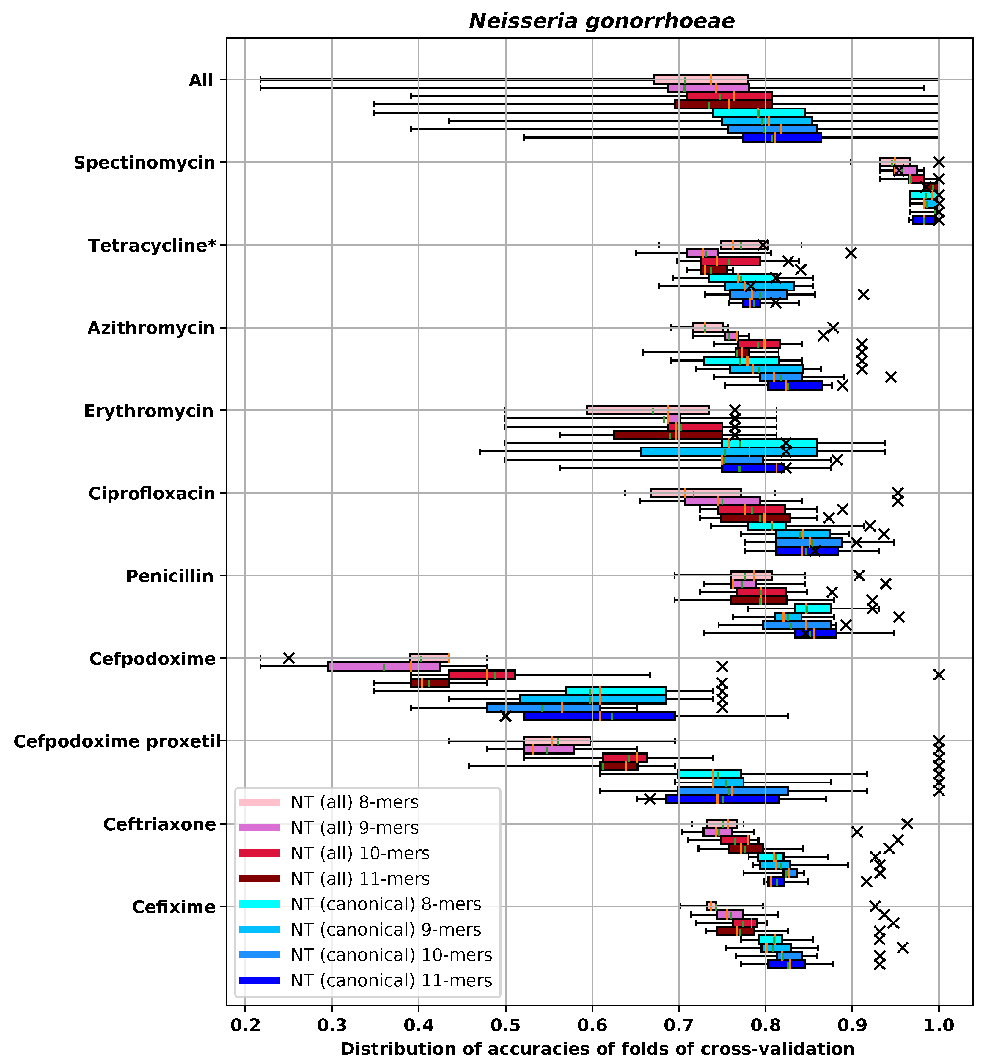
Appendix E.2. N. gonorrhoeae
| RMSE-CV | RMSE-H | DD1-CV | DD1-H | DD2-CV | DD2-H | ME-CV | ME-H | VME-CV | VME-H | |
|---|---|---|---|---|---|---|---|---|---|---|
| NT 8-mers | 0.87 (0.08) | 0.59 | 0.812 (0.026) | 0.927 | 0.959 (0.016) | 0.979 | 0.0 (0.0) | 0.0 | 0.0 (0.0) | 0.0 |
| NT 9-mers | 0.839 (0.074) | 0.538 | 0.818 (0.031) | 0.932 | 0.968 (0.014) | 0.995 | 0.0 (0.0) | 0.0 | 0.0 (0.0) | 0.0 |
| NT 10-mers | 0.846 (0.076) | 0.604 | 0.823 (0.019) | 0.932 | 0.966 (0.017) | 0.990 | 0.0 (0.0) | 0.0 | 0.0 (0.0) | 0.0 |
| NT 11-mers | 0.83 (0.068) | 0.571 | 0.814 (0.017) | 0.916 | 0.97 (0.013) | 0.990 | 0.0 (0.0) | 0.0 | 0.0 (0.0) | 0.0 |
| AA 3-mers | 0.891 (0.046) | 0.492 | 0.799 (0.026) | 0.921 | 0.957 (0.009) | 0.990 | 0.0 (0.0) | 0.0 | 0.0 (0.0) | 0.0 |
| AA 4-mers | 0.84 (0.075) | 0.596 | 0.812 (0.033) | 0.927 | 0.966 (0.01) | 0.984 | 0.0 (0.0) | 0.0 | 0.0 (0.0) | 0.0 |
| AA 5-mers | 0.796 (0.067) | 0.463 | 0.835 (0.023) | 0.963 | 0.974 (0.012) | 0.995 | 0.0 (0.0) | 0.0 | 0.0 (0.0) | 0.0 |
| Gene content | 0.873 (0.068) | 0.683 | 0.797 (0.024) | 0.895 | 0.961 (0.015) | 0.984 | 0.0 (0.0) | 0.0 | 0.0 (0.0) | 0.0 |
| SNP | 0.852 (0.071) | 0.673 | 0.812 (0.031) | 0.843 | 0.963 (0.018) | 0.995 | 0.0 (0.0) | 0.0 | 0.0 (0.0) | 0.0 |
| Gene + SNP | 0.86 (0.075) | 0.59 | 0.801 (0.033) | 0.916 | 0.965 (0.015) | 0.995 | 0.0 (0.0) | 0.0 | 0.0 (0.0) | 0.0 |
| RMSE-CV | RMSE-H | DD1-CV | DD1-H | DD2-CV | DD2-H | ME-CV | ME-H | VME-CV | VME-H | |
|---|---|---|---|---|---|---|---|---|---|---|
| NT 8-mers | 1.001 (0.141) | 0.774 | 0.771 (0.052) | 0.812 | 0.944 (0.018) | 0.971 | 0.006 (0.008) | 0.000 | 0.0 (0.0) | 0.0 |
| NT 9-mers | 0.979 (0.142) | 0.824 | 0.785 (0.053) | 0.783 | 0.939 (0.032) | 0.986 | 0.008 (0.008) | 0.000 | 0.0 (0.0) | 0.0 |
| NT 10-mers | 0.963 (0.131) | 0.694 | 0.794 (0.042) | 0.913 | 0.939 (0.032) | 0.971 | 0.005 (0.007) | 0.000 | 0.0 (0.0) | 0.0 |
| NT 11-mers | 0.967 (0.112) | 0.905 | 0.787 (0.023) | 0.812 | 0.942 (0.029) | 0.928 | 0.005 (0.007) | 0.000 | 0.0 (0.0) | 0.0 |
| AA 3-mers | 0.999 (0.134) | 0.861 | 0.787 (0.051) | 0.841 | 0.941 (0.029) | 0.928 | 0.005 (0.007) | 0.000 | 0.0 (0.0) | 0.0 |
| AA 4-mers | 1.029 (0.063) | 0.834 | 0.757 (0.026) | 0.87 | 0.936 (0.02) | 0.928 | 0.005 (0.007) | 0.000 | 0.0 (0.0) | 0.0 |
| AA 5-mers | 0.971 (0.116) | 0.838 | 0.791 (0.039) | 0.899 | 0.936 (0.02) | 0.957 | 0.003 (0.006) | 0.014 | 0.0 (0.0) | 0.0 |
| Gene content | 0.979 (0.132) | 0.666 | 0.768 (0.064) | 0.899 | 0.947 (0.033) | 0.986 | 0.005 (0.01) | 0.000 | 0.0 (0.0) | 0.0 |
| SNP | 1.034 (0.121) | 0.679 | 0.784 (0.031) | 0.884 | 0.926 (0.023) | 0.986 | 0.01 (0.011) | 0.000 | 0.0 (0.0) | 0.0 |
| Gene + SNP | 0.955 (0.107) | 0.724 | 0.779 (0.029) | 0.87 | 0.952 (0.026) | 0.971 | 0.005 (0.007) | 0.000 | 0.0 (0.0) | 0.0 |
| RMSE-CV | RMSE-H | DD1-CV | DD1-H | DD2-CV | DD2-H | ME-CV | ME-H | VME-CV | VME-H | |
|---|---|---|---|---|---|---|---|---|---|---|
| NT 8-mers | 1.196 (0.383) | 1.367 | 0.77 (0.115) | 0.824 | 0.938 (0.048) | 0.882 | - | - | - | - |
| NT 9-mers | 1.2 (0.426) | 1.314 | 0.753 (0.135) | 0.824 | 0.932 (0.051) | 0.941 | - | - | - | - |
| NT 10-mers | 1.166 (0.365) | 1.316 | 0.752 (0.1) | 0.882 | 0.932 (0.043) | 0.882 | - | - | - | - |
| NT 11-mers | 1.279 (0.362) | 1.476 | 0.77 (0.098) | 0.824 | 0.913 (0.064) | 0.941 | - | - | - | - |
| AA 3-mers | 1.371 (0.428) | 0.356 | 0.672 (0.1) | 0.941 | 0.864 (0.06) | 1.000 | - | - | - | - |
| AA 4-mers | 1.228 (0.311) | 1.595 | 0.733 (0.055) | 0.824 | 0.913 (0.03) | 0.882 | - | - | - | - |
| AA 5-mers | 1.17 (0.35) | 1.247 | 0.776 (0.057) | 0.882 | 0.938 (0.038) | 0.941 | - | - | - | - |
| Gene content | 1.263 (0.367) | 1.008 | 0.739 (0.088) | 0.706 | 0.913 (0.041) | 0.941 | - | - | - | - |
| SNP | 1.226 (0.402) | 0.669 | 0.752 (0.081) | 0.824 | 0.926 (0.067) | 1.000 | - | - | - | - |
| Gene + SNP | 1.277 (0.395) | 0.846 | 0.764 (0.061) | 0.882 | 0.913 (0.057) | 0.941 | - | - | - | - |
| RMSE-CV | RMSE-H | DD1-CV | DD1-H | DD2-CV | DD2-H | ME-CV | ME-H | VME-CV | VME-H | |
|---|---|---|---|---|---|---|---|---|---|---|
| NT 8-mers | 1.731 (0.328) | 1.064 | 0.597 (0.11) | 0.75 | 0.827 (0.062) | 0.75 | 0.0 (0.0) | 0.0 | 0.0 (0.0) | 0.0 |
| NT 9-mers | 1.699 (0.283) | 0.607 | 0.598 (0.099) | 0.75 | 0.831 (0.077) | 1.00 | 0.0 (0.0) | 0.0 | 0.0 (0.0) | 0.0 |
| NT 10-mers | 1.785 (0.283) | 1.037 | 0.542 (0.092) | 0.75 | 0.766 (0.079) | 1.00 | 0.0 (0.0) | 0.0 | 0.0 (0.0) | 0.0 |
| NT 11-mers | 1.698 (0.318) | 1.2 | 0.623 (0.102) | 0.50 | 0.809 (0.094) | 0.75 | 0.0 (0.0) | 0.0 | 0.0 (0.0) | 0.0 |
| AA 3-mers | 1.654 (0.307) | 1.558 | 0.572 (0.117) | 0.50 | 0.814 (0.056) | 0.75 | 0.0 (0.0) | 0.0 | 0.0 (0.0) | 0.0 |
| AA 4-mers | 1.625 (0.286) | 0.841 | 0.615 (0.073) | 0.75 | 0.823 (0.052) | 1.00 | 0.0 (0.0) | 0.0 | 0.0 (0.0) | 0.0 |
| AA 5-mers | 1.734 (0.261) | 1.402 | 0.593 (0.097) | 0.75 | 0.813 (0.059) | 0.75 | 0.0 (0.0) | 0.0 | 0.0 (0.0) | 0.0 |
| Gene content | 1.722 (0.281) | 0.903 | 0.528 (0.088) | 0.75 | 0.783 (0.065) | 1.00 | 0.0 (0.0) | 0.0 | 0.0 (0.0) | 0.0 |
| SNP | 1.662 (0.319) | 1.086 | 0.615 (0.086) | 0.25 | 0.827 (0.051) | 1.00 | 0.0 (0.0) | 0.0 | 0.0 (0.0) | 0.0 |
| Gene + SNP | 1.618 (0.34) | 1.126 | 0.602 (0.118) | 0.75 | 0.831 (0.069) | 0.75 | 0.0 (0.0) | 0.0 | 0.0 (0.0) | 0.0 |
| RMSE-CV | RMSE-H | DD1-CV | DD1-H | DD2-CV | DD2-H | ME-CV | ME-H | VME-CV | VME-H | |
|---|---|---|---|---|---|---|---|---|---|---|
| NT 8-mers | 0.352 (0.082) | 0.082 | 0.985 (0.016) | 1.000 | 0.995 (0.008) | 1.0 | 0.0 (0.0) | 0.0 | 0.0 (0.0) | 0.0 |
| NT 9-mers | 0.337 (0.101) | 0.109 | 0.986 (0.013) | 1.000 | 0.995 (0.011) | 1.0 | 0.0 (0.0) | 0.0 | 0.0 (0.0) | 0.0 |
| NT 10-mers | 0.305 (0.049) | 0.161 | 0.995 (0.011) | 1.000 | 0.998 (0.005) | 1.0 | 0.0 (0.0) | 0.0 | 0.0 (0.0) | 0.0 |
| NT 11-mers | 0.323 (0.057) | 0.148 | 0.983 (0.013) | 1.000 | 0.995 (0.008) | 1.0 | 0.0 (0.0) | 0.0 | 0.0 (0.0) | 0.0 |
| AA 3-mers | 0.38 (0.117) | 0.109 | 0.973 (0.022) | 1.000 | 0.995 (0.008) | 1.0 | 0.0 (0.0) | 0.0 | 0.0 (0.0) | 0.0 |
| AA 4-mers | 0.332 (0.088) | 0.227 | 0.98 (0.021) | 0.985 | 0.997 (0.007) | 1.0 | 0.0 (0.0) | 0.0 | 0.0 (0.0) | 0.0 |
| AA 5-mers | 0.332 (0.137) | 0.154 | 0.988 (0.015) | 1.000 | 0.997 (0.01) | 1.0 | 0.0 (0.0) | 0.0 | 0.0 (0.0) | 0.0 |
| Gene content | 0.36 (0.08) | 0.177 | 0.98 (0.015) | 1.000 | 0.997 (0.007) | 1.0 | 0.0 (0.0) | 0.0 | 0.0 (0.0) | 0.0 |
| SNP | 0.722 (0.183) | 0.224 | 0.889 (0.033) | 1.000 | 0.968 (0.025) | 1.0 | 0.0 (0.0) | 0.0 | 0.0 (0.0) | 0.0 |
| Gene + SNP | 0.402 (0.119) | 0.153 | 0.961 (0.022) | 1.000 | 0.997 (0.007) | 1.0 | 0.0 (0.0) | 0.0 | 0.0 (0.0) | 0.0 |
| RMSE-CV | RMSE-H | DD1-CV | DD1-H | DD2-CV | DD2-H | ME-CV | ME-H | VME-CV | VME-H | |
|---|---|---|---|---|---|---|---|---|---|---|
| NT 8-mers | 0.94 (0.076) | 0.637 | 0.81 (0.025) | 0.932 | 0.952 (0.014) | 0.989 | 0.0 (0.0) | 0.0 | 0.0 (0.0) | 0.0 |
| NT 9-mers | 0.944 (0.122) | 0.617 | 0.808 (0.029) | 0.958 | 0.953 (0.016) | 0.979 | 0.0 (0.0) | 0.0 | 0.0 (0.0) | 0.0 |
| NT 10-mers | 0.959 (0.069) | 0.635 | 0.82 (0.027) | 0.932 | 0.949 (0.011) | 0.974 | 0.0 (0.0) | 0.0 | 0.0 (0.0) | 0.0 |
| NT 11-mers | 0.91 (0.105) | 0.537 | 0.825 (0.03) | 0.932 | 0.956 (0.018) | 0.995 | 0.0 (0.0) | 0.0 | 0.0 (0.0) | 0.0 |
| AA 3-mers | 0.981 (0.12) | 0.456 | 0.809 (0.031) | 0.958 | 0.938 (0.02) | 0.984 | 0.0 (0.0) | 0.0 | 0.0 (0.0) | 0.0 |
| AA 4-mers | 0.895 (0.09) | 0.62 | 0.839 (0.029) | 0.937 | 0.953 (0.014) | 0.979 | 0.0 (0.0) | 0.0 | 0.0 (0.0) | 0.0 |
| AA 5-mers | 0.938 (0.098) | 0.535 | 0.819 (0.039) | 0.937 | 0.951 (0.015) | 0.979 | 0.0 (0.0) | 0.0 | 0.0 (0.0) | 0.0 |
| Gene content | 0.902 (0.084) | 0.754 | 0.821 (0.031) | 0.868 | 0.961 (0.014) | 0.974 | 0.0 (0.0) | 0.0 | 0.0 (0.0) | 0.0 |
| SNP | 0.943 (0.11) | 0.689 | 0.804 (0.036) | 0.879 | 0.953 (0.021) | 0.989 | 0.0 (0.0) | 0.0 | 0.0 (0.0) | 0.0 |
| Gene + SNP | 0.916 (0.078) | 0.66 | 0.811 (0.027) | 0.916 | 0.957 (0.011) | 0.968 | 0.0 (0.0) | 0.0 | 0.0 (0.0) | 0.0 |
| RMSE-CV | RMSE-H | DD1-CV | DD1-H | DD2-CV | DD2-H | ME-CV | ME-H | VME-CV | VME-H | |
|---|---|---|---|---|---|---|---|---|---|---|
| NT 8-mers | 1.146 (0.268) | 0.096 | 0.745 (0.079) | 1.000 | 0.935 (0.039) | 1.0 | 0.0 (0.0) | 0.0 | 0.0 (0.0) | 0.0 |
| NT 9-mers | 1.162 (0.196) | 0.096 | 0.754 (0.049) | 1.000 | 0.922 (0.038) | 1.0 | 0.0 (0.0) | 0.0 | 0.0 (0.0) | 0.0 |
| NT 10-mers | 1.119 (0.26) | 0.174 | 0.758 (0.099) | 1.000 | 0.913 (0.055) | 1.0 | 0.0 (0.0) | 0.0 | 0.0 (0.0) | 0.0 |
| NT 11-mers | 1.148 (0.236) | 0.849 | 0.75 (0.073) | 0.667 | 0.922 (0.043) | 1.0 | 0.0 (0.0) | 0.0 | 0.0 (0.0) | 0.0 |
| AA 3-mers | 1.143 (0.256) | 0.194 | 0.736 (0.085) | 1.000 | 0.914 (0.073) | 1.0 | 0.0 (0.0) | 0.0 | 0.0 (0.0) | 0.0 |
| AA 4-mers | 1.143 (0.282) | 0.143 | 0.732 (0.084) | 1.000 | 0.913 (0.062) | 1.0 | 0.0 (0.0) | 0.0 | 0.0 (0.0) | 0.0 |
| AA 5-mers | 1.117 (0.29) | 0.230 | 0.758 (0.092) | 1.000 | 0.922 (0.054) | 1.0 | 0.0 (0.0) | 0.0 | 0.0 (0.0) | 0.0 |
| Gene content | 1.122 (0.278) | 0.210 | 0.71 (0.108) | 1.000 | 0.918 (0.05) | 1.0 | 0.0 (0.0) | 0.0 | 0.0 (0.0) | 0.0 |
| SNP | 1.088 (0.267) | 0.180 | 0.784 (0.059) | 1.000 | 0.913 (0.034) | 1.0 | 0.0 (0.0) | 0.0 | 0.0 (0.0) | 0.0 |
| Gene + SNP | 1.104 (0.296) | 0.162 | 0.766 (0.079) | 1.000 | 0.931 (0.056) | 1.0 | 0.0 (0.0) | 0.0 | 0.0 (0.0) | 0.0 |
| RMSE-CV | RMSE-H | DD1-CV | DD1-H | DD2-CV | DD2-H | ME-CV | ME-H | VME-CV | VME-H | |
|---|---|---|---|---|---|---|---|---|---|---|
| NT 8-mers | 0.867 (0.093) | 0.648 | 0.848 (0.043) | 0.923 | 0.947 (0.019) | 0.985 | 0.0 (0.0) | 0.0 | 0.0 (0.0) | 0.0 |
| NT 9-mers | 0.903 (0.108) | 0.63 | 0.826 (0.034) | 0.954 | 0.944 (0.022) | 0.985 | 0.0 (0.0) | 0.0 | 0.0 (0.0) | 0.0 |
| NT 10-mers | 0.899 (0.125) | 0.583 | 0.829 (0.048) | 0.892 | 0.944 (0.025) | 1.000 | 0.0 (0.0) | 0.0 | 0.0 (0.0) | 0.0 |
| NT 11-mers | 0.894 (0.133) | 0.725 | 0.851 (0.057) | 0.846 | 0.945 (0.02) | 0.985 | 0.0 (0.0) | 0.0 | 0.0 (0.0) | 0.0 |
| AA 3-mers | 0.886 (0.133) | 0.59 | 0.836 (0.041) | 0.923 | 0.949 (0.026) | 0.954 | 0.0 (0.0) | 0.0 | 0.0 (0.0) | 0.0 |
| AA 4-mers | 0.83 (0.124) | 0.552 | 0.838 (0.064) | 0.908 | 0.956 (0.031) | 0.969 | 0.0 (0.0) | 0.0 | 0.0 (0.0) | 0.0 |
| AA 5-mers | 0.754 (0.112) | 0.529 | 0.855 (0.059) | 0.954 | 0.969 (0.017) | 0.969 | 0.0 (0.0) | 0.0 | 0.0 (0.0) | 0.0 |
| Gene content | 0.876 (0.102) | 0.61 | 0.821 (0.05) | 0.908 | 0.957 (0.035) | 1.000 | 0.0 (0.0) | 0.0 | 0.0 (0.0) | 0.0 |
| SNP | 0.923 (0.176) | 0.846 | 0.828 (0.046) | 0.877 | 0.942 (0.031) | 0.938 | 0.0 (0.0) | 0.0 | 0.0 (0.0) | 0.0 |
| Gene + SNP | 0.854 (0.149) | 0.788 | 0.836 (0.047) | 0.769 | 0.959 (0.028) | 1.000 | 0.0 (0.0) | 0.0 | 0.0 (0.0) | 0.0 |
| RMSE-CV | RMSE-H | DD1-CV | DD1-H | DD2-CV | DD2-H | ME-CV | ME-H | VME-CV | VME-H | |
|---|---|---|---|---|---|---|---|---|---|---|
| NT 8-mers | 1.271 (0.175) | 1.229 | 0.771 (0.052) | 0.911 | 0.906 (0.021) | 0.933 | 0.0 (0.0) | 0.0 | 0.0 (0.0) | 0.0 |
| NT 9-mers | 1.146 (0.226) | 0.815 | 0.793 (0.05) | 0.911 | 0.928 (0.018) | 0.967 | 0.0 (0.0) | 0.0 | 0.0 (0.0) | 0.0 |
| NT 10-mers | 1.093 (0.273) | 0.744 | 0.818 (0.046) | 0.944 | 0.935 (0.033) | 0.978 | 0.0 (0.0) | 0.0 | 0.0 (0.0) | 0.0 |
| NT 11-mers | 1.064 (0.202) | 0.636 | 0.826 (0.041) | 0.889 | 0.944 (0.025) | 0.989 | 0.0 (0.0) | 0.0 | 0.0 (0.0) | 0.0 |
| AA 3-mers | 1.31 (0.203) | 0.829 | 0.764 (0.028) | 0.900 | 0.912 (0.022) | 0.956 | 0.0 (0.0) | 0.0 | 0.0 (0.0) | 0.0 |
| AA 4-mers | 1.195 (0.239) | 0.747 | 0.789 (0.041) | 0.922 | 0.913 (0.027) | 0.989 | 0.0 (0.0) | 0.0 | 0.0 (0.0) | 0.0 |
| AA 5-mers | 1.245 (0.251) | 0.414 | 0.802 (0.046) | 0.944 | 0.92 (0.024) | 1.0 | 0.0 (0.0) | 0.0 | 0.0 (0.0) | 0.0 |
| Gene content | 1.225 (0.152) | 0.821 | 0.745 (0.02) | 0.867 | 0.911 (0.017) | 0.967 | 0.0 (0.0) | 0.0 | 0.0 (0.0) | 0.0 |
| SNP | 1.39 (0.161) | 0.712 | 0.718 (0.042) | 0.911 | 0.891 (0.017) | 0.978 | 0.0 (0.0) | 0.0 | 0.0 (0.0) | 0.0 |
| Gene + SNP | 1.241 (0.214) | 0.77 | 0.753 (0.038) | 0.944 | 0.912 (0.026) | 0.978 | 0.0 (0.0) | 0.0 | 0.0 (0.0) | 0.0 |
| RMSE-CV | RMSE-H | DD1-CV | DD1-H | DD2-CV | DD2-H | ME-CV | ME-H | VME-CV | VME-H | |
|---|---|---|---|---|---|---|---|---|---|---|
| NT 8-mers | 1.691 (0.594) | 1.44 | 0.807 (0.047) | 0.921 | 0.902 (0.05) | 0.984 | 0.012 (0.018) | 0.000 | 0.01 (0.009) | 0.016 |
| NT 9-mers | 1.4 (0.565) | 0.448 | 0.84 (0.043) | 0.937 | 0.941 (0.031) | 1.000 | 0.01 (0.012) | 0.000 | 0.007 (0.009) | 0.000 |
| NT 10-mers | 1.521 (0.5) | 0.547 | 0.854 (0.051) | 0.905 | 0.944 (0.023) | 0.968 | 0.01 (0.012) | 0.000 | 0.01 (0.012) | 0.000 |
| NT 11-mers | 1.563 (0.548) | 1.696 | 0.847 (0.049) | 0.857 | 0.939 (0.032) | 0.905 | 0.012 (0.008) | 0.032 | 0.012 (0.014) | 0.000 |
| AA 3-mers | 1.987 (0.836) | 1.526 | 0.828 (0.052) | 0.952 | 0.892 (0.052) | 0.968 | 0.016 (0.018) | 0.000 | 0.019 (0.02) | 0.016 |
| AA 4-mers | 1.403 (0.775) | 1.424 | 0.858 (0.033) | 0.952 | 0.939 (0.038) | 0.984 | 0.009 (0.012) | 0.000 | 0.009 (0.014) | 0.016 |
| AA 5-mers | 1.665 (0.698) | 1.235 | 0.885 (0.033) | 0.968 | 0.953 (0.036) | 0.984 | 0.017 (0.019) | 0.000 | 0.012 (0.011) | 0.016 |
| Gene content | 1.772 (0.567) | 0.484 | 0.802 (0.048) | 0.937 | 0.91 (0.032) | 1.000 | 0.017 (0.017) | 0.000 | 0.014 (0.017) | 0.000 |
| SNP | 1.54 (0.507) | 1.622 | 0.828 (0.03) | 0.889 | 0.929 (0.028) | 0.952 | 0.01 (0.012) | 0.000 | 0.004 (0.007) | 0.016 |
| Gene + SNP | 1.504 (0.422) | 0.745 | 0.838 (0.034) | 0.937 | 0.934 (0.03) | 0.968 | 0.009 (0.016) | 0.000 | 0.007 (0.012) | 0.000 |
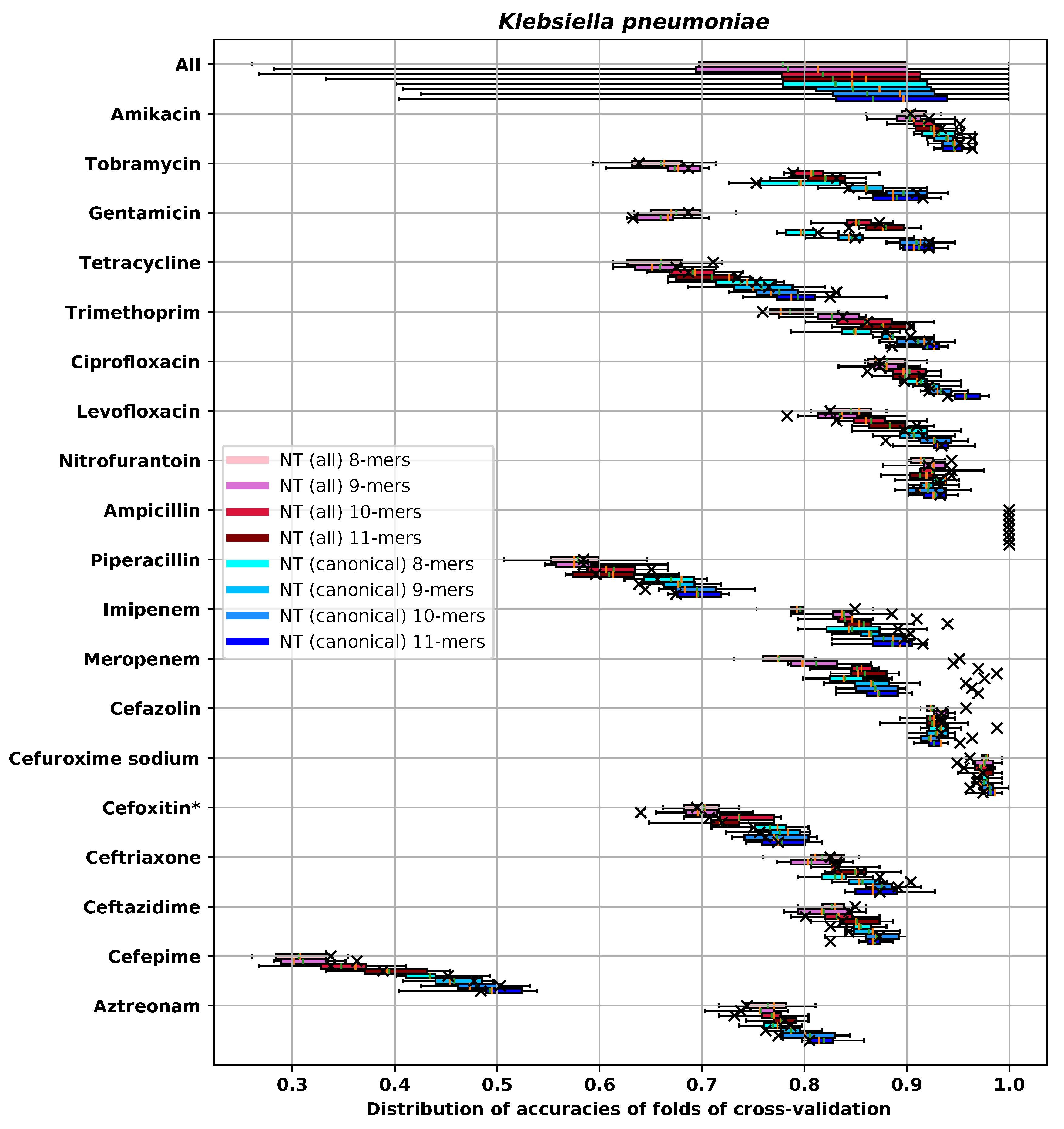
Appendix E.3. K. pneumoniae
| RMSE-CV | RMSE-H | DD1-CV | DD1-H | DD2-CV | DD2-H | ME-CV | ME-H | VME-CV | VME-H | |
|---|---|---|---|---|---|---|---|---|---|---|
| NT 8-mers | 1.128 (0.056) | 1.258 | 0.77 (0.017) | 0.787 | 0.903 (0.014) | 0.878 | 0.046 (0.008) | 0.067 | 0.007 (0.005) | 0.012 |
| NT 9-mers | 1.093 (0.081) | 1.22 | 0.787 (0.017) | 0.762 | 0.91 (0.015) | 0.866 | 0.045 (0.006) | 0.067 | 0.005 (0.004) | 0.006 |
| NT 10-mers | 1.057 (0.062) | 1.135 | 0.805 (0.026) | 0.774 | 0.914 (0.015) | 0.896 | 0.043 (0.008) | 0.049 | 0.007 (0.006) | 0.006 |
| NT 11-mers | 1.046 (0.08) | 1.064 | 0.819 (0.019) | 0.805 | 0.915 (0.017) | 0.902 | 0.043 (0.01) | 0.049 | 0.008 (0.009) | 0.006 |
| AA 3-mers | 1.129 (0.047) | 1.175 | 0.782 (0.018) | 0.774 | 0.896 (0.021) | 0.884 | 0.048 (0.01) | 0.055 | 0.005 (0.005) | 0.012 |
| AA 4-mers | 1.076 (0.081) | 1.161 | 0.801 (0.024) | 0.756 | 0.911 (0.012) | 0.890 | 0.043 (0.011) | 0.061 | 0.005 (0.006) | 0.006 |
| AA 5-mers | 1.022 (0.082) | 1.145 | 0.834 (0.024) | 0.793 | 0.922 (0.017) | 0.902 | 0.043 (0.014) | 0.055 | 0.005 (0.004) | 0.006 |
| Gene content | 1.037 (0.045) | 1.145 | 0.816 (0.021) | 0.811 | 0.918 (0.009) | 0.884 | 0.043 (0.014) | 0.061 | 0.003 (0.003) | 0.006 |
| SNP | 1.124 (0.085) | 1.199 | 0.798 (0.026) | 0.774 | 0.898 (0.016) | 0.884 | 0.047 (0.008) | 0.055 | 0.006 (0.008) | 0.006 |
| Gene + SNP | 1.106 (0.073) | 1.177 | 0.803 (0.024) | 0.787 | 0.901 (0.015) | 0.902 | 0.046 (0.011) | 0.079 | 0.008 (0.009) | 0.0 |
| RMSE-CV | RMSE-H | DD1-CV | DD1-H | DD2-CV | DD2-H | ME-CV | ME-H | VME-CV | VME-H | |
|---|---|---|---|---|---|---|---|---|---|---|
| NT 8-mers | 0.889 (0.049) | 0.907 | 0.766 (0.026) | 0.750 | 0.951 (0.017) | 0.945 | 0.001 (0.004) | 0.006 | 0.032 (0.012) | 0.037 |
| NT 9-mers | 0.894 (0.043) | 0.938 | 0.776 (0.026) | 0.756 | 0.948 (0.013) | 0.927 | 0.001 (0.002) | 0.000 | 0.04 (0.01) | 0.049 |
| NT 10-mers | 0.887 (0.061) | 0.918 | 0.773 (0.031) | 0.762 | 0.949 (0.017) | 0.945 | 0.001 (0.002) | 0.000 | 0.034 (0.009) | 0.037 |
| NT 11-mers | 0.9 (0.051) | 0.865 | 0.778 (0.024) | 0.774 | 0.945 (0.014) | 0.951 | 0.001 (0.002) | 0.000 | 0.037 (0.011) | 0.043 |
| AA 3-mers | 0.898 (0.039) | 0.976 | 0.758 (0.023) | 0.720 | 0.956 (0.014) | 0.945 | 0.001 (0.002) | 0.000 | 0.028 (0.013) | 0.037 |
| AA 4-mers | 0.865 (0.054) | 0.91 | 0.785 (0.028) | 0.750 | 0.955 (0.015) | 0.951 | 0.0 (0.0) | 0.000 | 0.029 (0.01) | 0.037 |
| AA 5-mers | 0.854 (0.053) | 0.887 | 0.788 (0.024) | 0.744 | 0.955 (0.011) | 0.951 | 0.001 (0.002) | 0.000 | 0.034 (0.013) | 0.043 |
| Gene content | 0.87 (0.047) | 0.866 | 0.766 (0.02) | 0.774 | 0.959 (0.016) | 0.963 | 0.0 (0.0) | 0.000 | 0.03 (0.013) | 0.018 |
| SNP | 0.885 (0.057) | 0.93 | 0.765 (0.034) | 0.768 | 0.959 (0.015) | 0.927 | 0.001 (0.002) | 0.000 | 0.032 (0.01) | 0.049 |
| Gene + SNP | 0.87 (0.065) | 0.905 | 0.77 (0.032) | 0.756 | 0.955 (0.016) | 0.951 | 0.001 (0.003) | 0.000 | 0.03 (0.009) | 0.037 |
| RMSE-CV | RMSE-H | DD1-CV | DD1-H | DD2-CV | DD2-H | ME-CV | ME-H | VME-CV | VME-H | |
|---|---|---|---|---|---|---|---|---|---|---|
| NT 8-mers | 0.934 (0.094) | 0.44 | 0.84 (0.024) | 0.976 | 0.948 (0.01) | 0.994 | 0.011 (0.009) | 0.000 | 0.004 (0.004) | 0.000 |
| NT 9-mers | 0.849 (0.128) | 0.564 | 0.867 (0.028) | 0.958 | 0.95 (0.015) | 0.982 | 0.012 (0.008) | 0.006 | 0.004 (0.004) | 0.006 |
| NT 10-mers | 0.846 (0.096) | 0.627 | 0.87 (0.024) | 0.964 | 0.951 (0.01) | 0.976 | 0.013 (0.008) | 0.012 | 0.003 (0.003) | 0.006 |
| NT 11-mers | 0.824 (0.126) | 0.528 | 0.873 (0.021) | 0.97 | 0.952 (0.018) | 0.988 | 0.012 (0.009) | 0.006 | 0.003 (0.003) | 0.006 |
| AA 3-mers | 0.996 (0.101) | 0.527 | 0.803 (0.034) | 0.952 | 0.933 (0.021) | 0.988 | 0.016 (0.01) | 0.000 | 0.01 (0.006) | 0.012 |
| AA 4-mers | 0.868 (0.098) | 0.529 | 0.869 (0.021) | 0.97 | 0.948 (0.014) | 0.982 | 0.015 (0.007) | 0.012 | 0.007 (0.006) | 0.000 |
| AA 5-mers | 0.794 (0.122) | 0.527 | 0.882 (0.023) | 0.958 | 0.956 (0.021) | 0.988 | 0.015 (0.009) | 0.006 | 0.004 (0.004) | 0.006 |
| Gene content | 0.845 (0.125) | 0.634 | 0.854 (0.03) | 0.945 | 0.95 (0.018) | 0.982 | 0.015 (0.011) | 0.000 | 0.005 (0.004) | 0.012 |
| SNP | 1.18 (0.109) | 0.85 | 0.762 (0.024) | 0.879 | 0.892 (0.02) | 0.945 | 0.026 (0.009) | 0.012 | 0.009 (0.005) | 0.006 |
| Gene + SNP | 0.889 (0.114) | 0.594 | 0.861 (0.031) | 0.952 | 0.945 (0.021) | 0.988 | 0.02 (0.011) | 0.000 | 0.006 (0.005) | 0.012 |
| RMSE-CV | RMSE-H | DD1-CV | DD1-H | DD2-CV | DD2-H | ME-CV | ME-H | VME-CV | VME-H | |
|---|---|---|---|---|---|---|---|---|---|---|
| NT 8-mers | 0.841 (0.075) | 0.925 | 0.795 (0.046) | 0.753 | 0.965 (0.012) | 0.934 | 0.0 (0.0) | 0.0 | 0.015 (0.008) | 0.054 |
| NT 9-mers | 0.73 (0.079) | 0.748 | 0.861 (0.03) | 0.843 | 0.972 (0.015) | 0.97 | 0.0 (0.0) | 0.0 | 0.015 (0.009) | 0.024 |
| NT 10-mers | 0.669 (0.079) | 0.693 | 0.897 (0.025) | 0.91 | 0.976 (0.012) | 0.952 | 0.0 (0.0) | 0.0 | 0.015 (0.008) | 0.042 |
| NT 11-mers | 0.644 (0.08) | 0.698 | 0.89 (0.027) | 0.916 | 0.981 (0.011) | 0.97 | 0.0 (0.0) | 0.0 | 0.011 (0.007) | 0.024 |
| AA 3-mers | 0.808 (0.046) | 0.802 | 0.803 (0.026) | 0.801 | 0.971 (0.011) | 0.976 | 0.0 (0.0) | 0.0 | 0.013 (0.008) | 0.018 |
| AA 4-mers | 0.667 (0.076) | 0.739 | 0.889 (0.033) | 0.861 | 0.976 (0.008) | 0.976 | 0.0 (0.0) | 0.0 | 0.014 (0.011) | 0.018 |
| AA 5-mers | 0.641 (0.055) | 0.671 | 0.904 (0.027) | 0.873 | 0.981 (0.007) | 0.982 | 0.0 (0.0) | 0.0 | 0.01 (0.006) | 0.012 |
| Gene content | 0.649 (0.063) | 0.668 | 0.9 (0.021) | 0.904 | 0.982 (0.009) | 0.976 | 0.0 (0.0) | 0.0 | 0.012 (0.007) | 0.018 |
| SNP | 0.856 (0.089) | 0.891 | 0.797 (0.037) | 0.801 | 0.953 (0.019) | 0.964 | 0.001 (0.002) | 0.0 | 0.023 (0.014) | 0.024 |
| Gene + SNP | 0.625 (0.081) | 0.7 | 0.909 (0.017) | 0.886 | 0.979 (0.013) | 0.97 | 0.0 (0.0) | 0.0 | 0.012 (0.008) | 0.024 |
| RMSE-CV | RMSE-H | DD1-CV | DD1-H | DD2-CV | DD2-H | ME-CV | ME-H | VME-CV | VME-H | |
|---|---|---|---|---|---|---|---|---|---|---|
| NT 8-mers | 0.879 (0.043) | 0.812 | 0.799 (0.02) | 0.813 | 0.943 (0.011) | 0.952 | 0.001 (0.002) | 0.000 | 0.038 (0.01) | 0.042 |
| NT 9-mers | 0.781 (0.055) | 0.762 | 0.847 (0.027) | 0.849 | 0.958 (0.015) | 0.964 | 0.001 (0.002) | 0.000 | 0.027 (0.011) | 0.030 |
| NT 10-mers | 0.676 (0.068) | 0.585 | 0.909 (0.021) | 0.922 | 0.966 (0.01) | 0.982 | 0.002 (0.003) | 0.000 | 0.022 (0.006) | 0.018 |
| NT 11-mers | 0.629 (0.053) | 0.546 | 0.912 (0.018) | 0.922 | 0.973 (0.01) | 0.982 | 0.001 (0.002) | 0.000 | 0.019 (0.006) | 0.018 |
| AA 3-mers | 0.869 (0.07) | 0.851 | 0.789 (0.028) | 0.765 | 0.951 (0.023) | 0.964 | 0.001 (0.003) | 0.006 | 0.028 (0.014) | 0.018 |
| AA 4-mers | 0.664 (0.075) | 0.646 | 0.905 (0.022) | 0.880 | 0.973 (0.012) | 0.982 | 0.001 (0.003) | 0.000 | 0.017 (0.004) | 0.012 |
| AA 5-mers | 0.608 (0.081) | 0.57 | 0.924 (0.026) | 0.910 | 0.975 (0.01) | 0.988 | 0.001 (0.003) | 0.000 | 0.015 (0.007) | 0.012 |
| Gene content | 0.634 (0.044) | 0.557 | 0.913 (0.017) | 0.922 | 0.975 (0.011) | 0.982 | 0.001 (0.002) | 0.000 | 0.019 (0.007) | 0.018 |
| SNP | 0.766 (0.075) | 0.657 | 0.873 (0.027) | 0.916 | 0.951 (0.018) | 0.964 | 0.001 (0.003) | 0.000 | 0.033 (0.012) | 0.030 |
| Gene + SNP | 0.636 (0.039) | 0.587 | 0.926 (0.011) | 0.904 | 0.972 (0.008) | 0.988 | 0.0 (0.0) | 0.000 | 0.021 (0.007) | 0.012 |
| RMSE-CV | RMSE-H | DD1-CV | DD1-H | DD2-CV | DD2-H | ME-CV | ME-H | VME-CV | VME-H | |
|---|---|---|---|---|---|---|---|---|---|---|
| NT 8-mers | 0.91 (0.131) | 0.758 | 0.847 (0.037) | 0.892 | 0.94 (0.024) | 0.97 | 0.019 (0.014) | 0.006 | 0.005 (0.004) | 0.000 |
| NT 9-mers | 0.845 (0.095) | 0.773 | 0.865 (0.019) | 0.904 | 0.949 (0.019) | 0.964 | 0.019 (0.01) | 0.012 | 0.005 (0.008) | 0.000 |
| NT 10-mers | 0.831 (0.098) | 0.725 | 0.877 (0.026) | 0.898 | 0.954 (0.018) | 0.958 | 0.019 (0.011) | 0.006 | 0.002 (0.004) | 0.000 |
| NT 11-mers | 0.819 (0.099) | 0.771 | 0.886 (0.027) | 0.916 | 0.951 (0.023) | 0.97 | 0.019 (0.013) | 0.012 | 0.005 (0.007) | 0.000 |
| AA 3-mers | 0.97 (0.099) | 0.74 | 0.824 (0.032) | 0.898 | 0.933 (0.022) | 0.97 | 0.02 (0.015) | 0.0 | 0.009 (0.007) | 0.000 |
| AA 4-mers | 0.827 (0.099) | 0.63 | 0.883 (0.024) | 0.916 | 0.953 (0.017) | 0.982 | 0.021 (0.011) | 0.006 | 0.005 (0.004) | 0.006 |
| AA 5-mers | 0.799 (0.104) | 0.751 | 0.878 (0.027) | 0.922 | 0.958 (0.02) | 0.964 | 0.019 (0.014) | 0.012 | 0.005 (0.006) | 0.006 |
| Gene content | 0.825 (0.084) | 0.708 | 0.874 (0.029) | 0.892 | 0.956 (0.017) | 0.97 | 0.021 (0.012) | 0.018 | 0.003 (0.004) | 0.000 |
| SNP | 1.053 (0.087) | 0.93 | 0.789 (0.03) | 0.801 | 0.921 (0.021) | 0.964 | 0.034 (0.016) | 0.018 | 0.006 (0.007) | 0.012 |
| Gene + SNP | 0.82 (0.105) | 0.78 | 0.872 (0.026) | 0.916 | 0.956 (0.02) | 0.964 | 0.02 (0.012) | 0.018 | 0.006 (0.008) | 0.006 |
| RMSE-CV | RMSE-H | DD1-CV | DD1-H | DD2-CV | DD2-H | ME-CV | ME-H | VME-CV | VME-H | |
|---|---|---|---|---|---|---|---|---|---|---|
| NT 8-mers | 0.584 (0.108) | 0.599 | 0.905 (0.027) | 0.898 | 0.977 (0.02) | 0.988 | 0.0 (0.0) | 0.0 | 0.0 (0.0) | 0.0 |
| NT 9-mers | 0.57 (0.077) | 0.539 | 0.907 (0.021) | 0.916 | 0.979 (0.014) | 0.988 | 0.0 (0.0) | 0.0 | 0.0 (0.0) | 0.0 |
| NT 10-mers | 0.553 (0.093) | 0.627 | 0.927 (0.02) | 0.880 | 0.979 (0.014) | 0.976 | 0.0 (0.0) | 0.0 | 0.0 (0.0) | 0.0 |
| NT 11-mers | 0.523 (0.113) | 0.494 | 0.932 (0.019) | 0.934 | 0.977 (0.018) | 0.982 | 0.0 (0.0) | 0.0 | 0.0 (0.0) | 0.0 |
| AA 3-mers | 0.613 (0.07) | 0.605 | 0.901 (0.018) | 0.886 | 0.976 (0.015) | 0.976 | 0.0 (0.0) | 0.0 | 0.0 (0.0) | 0.0 |
| AA 4-mers | 0.559 (0.068) | 0.656 | 0.92 (0.014) | 0.880 | 0.978 (0.01) | 0.970 | 0.0 (0.0) | 0.0 | 0.0 (0.0) | 0.0 |
| AA 5-mers | 0.51 (0.086) | 0.548 | 0.937 (0.021) | 0.928 | 0.979 (0.011) | 0.970 | 0.0 (0.0) | 0.0 | 0.0 (0.0) | 0.0 |
| Gene content | 0.56 (0.06) | 0.553 | 0.918 (0.018) | 0.940 | 0.98 (0.012) | 0.976 | 0.0 (0.0) | 0.0 | 0.0 (0.0) | 0.0 |
| SNP | 0.549 (0.06) | 0.576 | 0.929 (0.017) | 0.910 | 0.977 (0.009) | 0.970 | 0.0 (0.0) | 0.0 | 0.0 (0.0) | 0.0 |
| Gene + SNP | 0.514 (0.113) | 0.538 | 0.938 (0.022) | 0.940 | 0.98 (0.014) | 0.970 | 0.0 (0.0) | 0.0 | 0.0 (0.0) | 0.0 |
| RMSE-CV | RMSE-H | DD1-CV | DD1-H | DD2-CV | DD2-H | ME-CV | ME-H | VME-CV | VME-H | |
|---|---|---|---|---|---|---|---|---|---|---|
| NT 8-mers | 0.575 (0.069) | 0.504 | 0.929 (0.019) | 0.933 | 0.985 (0.007) | 1.000 | 0.0 (0.0) | 0.0 | 0.004 (0.006) | 0.000 |
| NT 9-mers | 0.58 (0.065) | 0.516 | 0.922 (0.014) | 0.933 | 0.986 (0.007) | 1.000 | 0.0 (0.0) | 0.0 | 0.002 (0.005) | 0.000 |
| NT 10-mers | 0.613 (0.075) | 0.646 | 0.921 (0.027) | 0.91 | 0.979 (0.011) | 0.989 | 0.0 (0.0) | 0.0 | 0.007 (0.01) | 0.011 |
| NT 11-mers | 0.576 (0.046) | 0.581 | 0.928 (0.015) | 0.933 | 0.984 (0.008) | 0.989 | 0.0 (0.0) | 0.0 | 0.005 (0.008) | 0.011 |
| AA 3-mers | 0.58 (0.037) | 0.531 | 0.927 (0.019) | 0.921 | 0.984 (0.008) | 1.000 | 0.001 (0.004) | 0.0 | 0.002 (0.005) | 0.000 |
| AA 4-mers | 0.565 (0.051) | 0.46 | 0.932 (0.027) | 0.966 | 0.983 (0.006) | 1.000 | 0.001 (0.004) | 0.0 | 0.002 (0.005) | 0.000 |
| AA 5-mers | 0.535 (0.044) | 0.469 | 0.944 (0.02) | 0.944 | 0.988 (0.008) | 1.000 | 0.0 (0.0) | 0.0 | 0.001 (0.004) | 0.000 |
| Gene content | 0.558 (0.044) | 0.482 | 0.933 (0.016) | 0.955 | 0.985 (0.007) | 1.000 | 0.0 (0.0) | 0.0 | 0.001 (0.004) | 0.000 |
| SNP | 0.528 (0.055) | 0.549 | 0.943 (0.02) | 0.921 | 0.989 (0.007) | 1.000 | 0.0 (0.0) | 0.0 | 0.001 (0.004) | 0.000 |
| Gene + SNP | 0.539 (0.066) | 0.555 | 0.94 (0.015) | 0.91 | 0.988 (0.01) | 1.000 | 0.0 (0.0) | 0.0 | 0.001 (0.004) | 0.000 |
| RMSE-CV | RMSE-H | DD1-CV | DD1-H | DD2-CV | DD2-H | ME-CV | ME-H | VME-CV | VME-H | |
|---|---|---|---|---|---|---|---|---|---|---|
| NT 8-mers | 0.111 (0.013) | 0.084 | 1.0 (0.0) | 1.0 | 1.0 (0.0) | 1.0 | 0.0 (0.0) | 0.0 | 0.0 (0.0) | 0.0 |
| NT 9-mers | 0.108 (0.012) | 0.11 | 1.0 (0.0) | 1.0 | 1.0 (0.0) | 1.0 | 0.0 (0.0) | 0.0 | 0.0 (0.0) | 0.0 |
| NT 10-mers | 0.12 (0.008) | 0.083 | 1.0 (0.0) | 1.0 | 1.0 (0.0) | 1.0 | 0.0 (0.0) | 0.0 | 0.0 (0.0) | 0.0 |
| NT 11-mers | 0.107 (0.012) | 0.106 | 1.0 (0.0) | 1.0 | 1.0 (0.0) | 1.0 | 0.0 (0.0) | 0.0 | 0.0 (0.0) | 0.0 |
| AA 3-mers | 0.111 (0.014) | 0.096 | 1.0 (0.0) | 1.0 | 1.0 (0.0) | 1.0 | 0.0 (0.0) | 0.0 | 0.0 (0.0) | 0.0 |
| AA 4-mers | 0.108 (0.007) | 0.105 | 1.0 (0.0) | 1.0 | 1.0 (0.0) | 1.0 | 0.0 (0.0) | 0.0 | 0.0 (0.0) | 0.0 |
| AA 5-mers | 0.113 (0.009) | 0.098 | 1.0 (0.0) | 1.0 | 1.0 (0.0) | 1.0 | 0.0 (0.0) | 0.0 | 0.0 (0.0) | 0.0 |
| Gene content | 0.107 (0.008) | 0.118 | 1.0 (0.0) | 1.0 | 1.0 (0.0) | 1.0 | 0.0 (0.0) | 0.0 | 0.0 (0.0) | 0.0 |
| SNP | 0.115 (0.002) | 0.143 | 1.0 (0.0) | 1.0 | 1.0 (0.0) | 1.0 | 0.0 (0.0) | 0.0 | 0.0 (0.0) | 0.0 |
| Gene + SNP | 0.109 (0.012) | 0.104 | 1.0 (0.0) | 1.0 | 1.0 (0.0) | 1.0 | 0.0 (0.0) | 0.0 | 0.0 (0.0) | 0.0 |
| RMSE-CV | RMSE-H | DD1-CV | DD1-H | DD2-CV | DD2-H | ME-CV | ME-H | VME-CV | VME-H | |
|---|---|---|---|---|---|---|---|---|---|---|
| NT 8-mers | 0.95 (0.042) | 0.966 | 0.738 (0.039) | 0.753 | 0.949 (0.012) | 0.928 | 0.0 (0.0) | 0.0 | 0.025 (0.01) | 0.036 |
| NT 9-mers | 0.897 (0.053) | 0.899 | 0.758 (0.04) | 0.765 | 0.957 (0.01) | 0.970 | 0.001 (0.002) | 0.0 | 0.025 (0.009) | 0.018 |
| NT 10-mers | 0.846 (0.043) | 0.761 | 0.775 (0.032) | 0.831 | 0.971 (0.009) | 0.970 | 0.001 (0.003) | 0.0 | 0.017 (0.01) | 0.018 |
| NT 11-mers | 0.844 (0.056) | 0.792 | 0.793 (0.037) | 0.825 | 0.966 (0.01) | 0.964 | 0.001 (0.003) | 0.0 | 0.021 (0.009) | 0.036 |
| AA 3-mers | 0.95 (0.044) | 0.894 | 0.725 (0.036) | 0.747 | 0.96 (0.015) | 0.952 | 0.001 (0.003) | 0.0 | 0.011 (0.011) | 0.024 |
| AA 4-mers | 0.847 (0.04) | 0.844 | 0.791 (0.041) | 0.801 | 0.959 (0.008) | 0.958 | 0.001 (0.003) | 0.0 | 0.023 (0.006) | 0.030 |
| AA 5-mers | 0.798 (0.047) | 0.722 | 0.804 (0.025) | 0.855 | 0.977 (0.01) | 0.970 | 0.0 (0.0) | 0.0 | 0.014 (0.01) | 0.024 |
| Gene content | 0.79 (0.048) | 0.795 | 0.794 (0.041) | 0.837 | 0.977 (0.007) | 0.970 | 0.001 (0.003) | 0.0 | 0.014 (0.004) | 0.030 |
| SNP | 1.022 (0.068) | 0.997 | 0.69 (0.041) | 0.729 | 0.949 (0.014) | 0.946 | 0.001 (0.002) | 0.0 | 0.015 (0.009) | 0.030 |
| Gene + SNP | 0.812 (0.049) | 0.785 | 0.793 (0.041) | 0.861 | 0.969 (0.007) | 0.964 | 0.001 (0.003) | 0.0 | 0.021 (0.009) | 0.024 |
| RMSE-CV | RMSE-H | DD1-CV | DD1-H | DD2-CV | DD2-H | ME-CV | ME-H | VME-CV | VME-H | |
|---|---|---|---|---|---|---|---|---|---|---|
| NT 8-mers | 1.016 (0.097) | 0.955 | 0.855 (0.014) | 0.825 | 0.929 (0.016) | 0.916 | 0.017 (0.008) | 0.018 | 0.008 (0.006) | 0.000 |
| NT 9-mers | 0.975 (0.134) | 0.861 | 0.863 (0.016) | 0.843 | 0.937 (0.009) | 0.94 | 0.011 (0.011) | 0.012 | 0.008 (0.005) | 0.000 |
| NT 10-mers | 0.953 (0.132) | 0.719 | 0.871 (0.025) | 0.873 | 0.935 (0.019) | 0.964 | 0.007 (0.007) | 0.018 | 0.012 (0.008) | 0.000 |
| NT 11-mers | 0.906 (0.1) | 0.834 | 0.869 (0.009) | 0.825 | 0.948 (0.014) | 0.946 | 0.006 (0.007) | 0.012 | 0.007 (0.008) | 0.000 |
| AA 3-mers | 1.1 (0.093) | 0.928 | 0.839 (0.022) | 0.843 | 0.921 (0.014) | 0.928 | 0.017 (0.01) | 0.012 | 0.008 (0.008) | 0.000 |
| AA 4-mers | 0.977 (0.112) | 0.778 | 0.865 (0.02) | 0.867 | 0.938 (0.014) | 0.952 | 0.01 (0.007) | 0.012 | 0.01 (0.01) | 0.000 |
| AA 5-mers | 0.877 (0.122) | 0.712 | 0.885 (0.016) | 0.88 | 0.955 (0.014) | 0.97 | 0.006 (0.006) | 0.018 | 0.011 (0.008) | 0.000 |
| Gene content | 0.889 (0.112) | 0.706 | 0.885 (0.017) | 0.904 | 0.947 (0.017) | 0.964 | 0.007 (0.006) | 0.018 | 0.005 (0.004) | 0.000 |
| SNP | 1.06 (0.101) | 1.021 | 0.862 (0.017) | 0.88 | 0.925 (0.014) | 0.928 | 0.01 (0.006) | 0.030 | 0.015 (0.008) | 0.006 |
| Gene + SNP | 0.959 (0.105) | 0.911 | 0.871 (0.014) | 0.855 | 0.939 (0.015) | 0.934 | 0.007 (0.008) | 0.018 | 0.009 (0.006) | 0.012 |
| RMSE-CV | RMSE-H | DD1-CV | DD1-H | DD2-CV | DD2-H | ME-CV | ME-H | VME-CV | VME-H | |
|---|---|---|---|---|---|---|---|---|---|---|
| NT 8-mers | 0.522 (0.045) | 0.408 | 0.931 (0.02) | 0.952 | 0.989 (0.007) | 0.994 | 0.0 (0.0) | 0.0 | 0.007 (0.005) | 0.006 |
| NT 9-mers | 0.505 (0.057) | 0.384 | 0.939 (0.014) | 0.964 | 0.989 (0.009) | 1.000 | 0.0 (0.0) | 0.0 | 0.007 (0.005) | 0.000 |
| NT 10-mers | 0.476 (0.058) | 0.375 | 0.945 (0.015) | 0.952 | 0.991 (0.007) | 1.000 | 0.0 (0.0) | 0.0 | 0.006 (0.006) | 0.000 |
| NT 11-mers | 0.478 (0.063) | 0.341 | 0.946 (0.012) | 0.964 | 0.989 (0.008) | 1.000 | 0.0 (0.0) | 0.0 | 0.006 (0.005) | 0.000 |
| AA 3-mers | 0.521 (0.07) | 0.431 | 0.931 (0.022) | 0.934 | 0.989 (0.01) | 1.000 | 0.0 (0.0) | 0.0 | 0.007 (0.005) | 0.000 |
| AA 4-mers | 0.488 (0.07) | 0.361 | 0.942 (0.014) | 0.982 | 0.989 (0.009) | 1.000 | 0.0 (0.0) | 0.0 | 0.006 (0.006) | 0.000 |
| AA 5-mers | 0.48 (0.063) | 0.323 | 0.944 (0.019) | 0.988 | 0.991 (0.006) | 1.000 | 0.0 (0.0) | 0.0 | 0.005 (0.005) | 0.000 |
| Gene content | 0.5 (0.07) | 0.369 | 0.942 (0.014) | 0.964 | 0.987 (0.012) | 1.000 | 0.0 (0.0) | 0.0 | 0.007 (0.005) | 0.000 |
| SNP | 0.549 (0.057) | 0.455 | 0.934 (0.021) | 0.958 | 0.986 (0.008) | 0.994 | 0.0 (0.0) | 0.0 | 0.008 (0.005) | 0.006 |
| Gene + SNP | 0.494 (0.067) | 0.363 | 0.945 (0.018) | 0.97 | 0.989 (0.007) | 0.994 | 0.0 (0.0) | 0.0 | 0.007 (0.005) | 0.006 |
| RMSE-CV | RMSE-H | DD1-CV | DD1-H | DD2-CV | DD2-H | ME-CV | ME-H | VME-CV | VME-H | |
|---|---|---|---|---|---|---|---|---|---|---|
| NT 8-mers | 1.139 (0.137) | 0.73 | 0.83 (0.021) | 0.873 | 0.913 (0.021) | 0.97 | 0.012 (0.008) | 0.000 | 0.0 (0.0) | 0.0 |
| NT 9-mers | 0.999 (0.125) | 0.682 | 0.857 (0.019) | 0.904 | 0.929 (0.017) | 0.958 | 0.009 (0.008) | 0.006 | 0.001 (0.002) | 0.0 |
| NT 10-mers | 0.891 (0.131) | 0.68 | 0.875 (0.016) | 0.892 | 0.949 (0.014) | 0.958 | 0.006 (0.006) | 0.000 | 0.001 (0.003) | 0.0 |
| NT 11-mers | 0.862 (0.129) | 0.789 | 0.873 (0.026) | 0.873 | 0.947 (0.019) | 0.946 | 0.003 (0.004) | 0.006 | 0.0 (0.0) | 0.0 |
| AA 3-mers | 1.136 (0.112) | 0.92 | 0.839 (0.008) | 0.867 | 0.909 (0.013) | 0.958 | 0.016 (0.01) | 0.012 | 0.0 (0.0) | 0.0 |
| AA 4-mers | 0.937 (0.2) | 0.674 | 0.88 (0.025) | 0.898 | 0.946 (0.023) | 0.97 | 0.011 (0.009) | 0.000 | 0.003 (0.004) | 0.0 |
| AA 5-mers | 0.749 (0.142) | 0.444 | 0.916 (0.026) | 0.958 | 0.963 (0.016) | 0.988 | 0.003 (0.003) | 0.000 | 0.001 (0.002) | 0.0 |
| Gene content | 0.893 (0.096) | 0.651 | 0.867 (0.027) | 0.922 | 0.937 (0.01) | 0.97 | 0.015 (0.008) | 0.000 | 0.0 (0.0) | 0.0 |
| SNP | 1.255 (0.121) | 0.923 | 0.831 (0.017) | 0.849 | 0.898 (0.01) | 0.946 | 0.031 (0.009) | 0.018 | 0.0 (0.0) | 0.0 |
| Gene + SNP | 0.89 (0.123) | 0.84 | 0.891 (0.026) | 0.898 | 0.951 (0.015) | 0.952 | 0.006 (0.007) | 0.000 | 0.0 (0.0) | 0.0 |
| RMSE-CV | RMSE-H | DD1-CV | DD1-H | DD2-CV | DD2-H | ME-CV | ME-H | VME-CV | VME-H | |
|---|---|---|---|---|---|---|---|---|---|---|
| NT 8-mers | 0.335 (0.069) | 0.391 | 0.978 (0.007) | 0.968 | 0.99 (0.006) | 0.987 | 0.0 (0.0) | 0.0 | 0.001 (0.002) | 0.000 |
| NT 9-mers | 0.34 (0.065) | 0.366 | 0.975 (0.009) | 0.968 | 0.992 (0.005) | 0.994 | 0.001 (0.002) | 0.0 | 0.0 (0.0) | 0.000 |
| NT 10-mers | 0.325 (0.079) | 0.471 | 0.981 (0.009) | 0.962 | 0.992 (0.007) | 0.981 | 0.0 (0.0) | 0.0 | 0.0 (0.0) | 0.000 |
| NT 11-mers | 0.322 (0.048) | 0.361 | 0.982 (0.009) | 0.975 | 0.991 (0.006) | 0.994 | 0.0 (0.0) | 0.0 | 0.0 (0.0) | 0.000 |
| AA 3-mers | 0.362 (0.064) | 0.378 | 0.968 (0.011) | 0.968 | 0.992 (0.008) | 0.987 | 0.0 (0.0) | 0.0 | 0.0 (0.0) | 0.000 |
| AA 4-mers | 0.323 (0.048) | 0.422 | 0.978 (0.006) | 0.968 | 0.992 (0.005) | 0.987 | 0.0 (0.0) | 0.0 | 0.0 (0.0) | 0.000 |
| AA 5-mers | 0.327 (0.05) | 0.475 | 0.98 (0.008) | 0.962 | 0.993 (0.004) | 0.981 | 0.001 (0.002) | 0.0 | 0.0 (0.0) | 0.006 |
| Gene content | 0.377 (0.059) | 0.424 | 0.968 (0.008) | 0.955 | 0.989 (0.007) | 0.987 | 0.0 (0.0) | 0.0 | 0.0 (0.0) | 0.000 |
| SNP | 0.499 (0.063) | 0.477 | 0.933 (0.014) | 0.911 | 0.982 (0.012) | 0.994 | 0.0 (0.0) | 0.0 | 0.0 (0.0) | 0.000 |
| Gene + SNP | 0.398 (0.069) | 0.371 | 0.968 (0.011) | 0.975 | 0.986 (0.009) | 0.987 | 0.0 (0.0) | 0.0 | 0.0 (0.0) | 0.000 |
| RMSE-CV | RMSE-H | DD1-CV | DD1-H | DD2-CV | DD2-H | ME-CV | ME-H | VME-CV | VME-H | |
|---|---|---|---|---|---|---|---|---|---|---|
| NT 8-mers | 0.658 (0.132) | 0.249 | 0.932 (0.011) | 0.988 | 0.966 (0.015) | 1.0 | 0.005 (0.005) | 0.000 | 0.013 (0.008) | 0.0 |
| NT 9-mers | 0.627 (0.125) | 0.442 | 0.928 (0.015) | 0.934 | 0.966 (0.014) | 0.994 | 0.003 (0.003) | 0.000 | 0.021 (0.013) | 0.018 |
| NT 10-mers | 0.662 (0.1) | 0.403 | 0.921 (0.014) | 0.964 | 0.965 (0.009) | 0.994 | 0.001 (0.003) | 0.000 | 0.019 (0.009) | 0.006 |
| NT 11-mers | 0.628 (0.083) | 0.475 | 0.927 (0.011) | 0.952 | 0.968 (0.01) | 0.982 | 0.001 (0.002) | 0.000 | 0.024 (0.01) | 0.024 |
| AA 3-mers | 0.814 (0.069) | 0.582 | 0.915 (0.01) | 0.934 | 0.951 (0.009) | 0.976 | 0.007 (0.006) | 0.000 | 0.021 (0.012) | 0.006 |
| AA 4-mers | 0.658 (0.102) | 0.416 | 0.939 (0.02) | 0.952 | 0.963 (0.013) | 0.988 | 0.002 (0.003) | 0.000 | 0.014 (0.011) | 0.012 |
| AA 5-mers | 0.592 (0.136) | 0.445 | 0.939 (0.017) | 0.964 | 0.971 (0.015) | 0.988 | 0.001 (0.003) | 0.000 | 0.015 (0.01) | 0.006 |
| Gene content | 0.627 (0.154) | 0.569 | 0.937 (0.024) | 0.952 | 0.969 (0.014) | 0.982 | 0.003 (0.005) | 0.000 | 0.011 (0.007) | 0.012 |
| SNP | 0.847 (0.094) | 0.628 | 0.898 (0.023) | 0.934 | 0.947 (0.012) | 0.958 | 0.008 (0.005) | 0.006 | 0.037 (0.02) | 0.042 |
| Gene + SNP | 0.719 (0.161) | 0.406 | 0.928 (0.024) | 0.952 | 0.958 (0.02) | 0.994 | 0.009 (0.007) | 0.000 | 0.017 (0.013) | 0.018 |
| RMSE-CV | RMSE-H | DD1-CV | DD1-H | DD2-CV | DD2-H | ME-CV | ME-H | VME-CV | VME-H | |
|---|---|---|---|---|---|---|---|---|---|---|
| NT 8-mers | 1.961 (0.075) | 1.744 | 0.434 (0.028) | 0.452 | 0.679 (0.021) | 0.726 | 0.03 (0.008) | 0.013 | 0.018 (0.012) | 0.006 |
| NT 9-mers | 1.91 (0.067) | 1.73 | 0.458 (0.027) | 0.478 | 0.698 (0.024) | 0.701 | 0.024 (0.007) | 0.006 | 0.018 (0.008) | 0.006 |
| NT 10-mers | 1.871 (0.064) | 1.796 | 0.481 (0.03) | 0.503 | 0.721 (0.016) | 0.72 | 0.025 (0.013) | 0.006 | 0.018 (0.005) | 0.006 |
| NT 11-mers | 1.842 (0.079) | 1.677 | 0.493 (0.039) | 0.484 | 0.722 (0.019) | 0.732 | 0.028 (0.012) | 0.013 | 0.015 (0.014) | 0.000 |
| AA 3-mers | 1.982 (0.077) | 1.793 | 0.41 (0.024) | 0.420 | 0.665 (0.042) | 0.72 | 0.027 (0.009) | 0.006 | 0.014 (0.011) | 0.006 |
| AA 4-mers | 1.863 (0.089) | 1.617 | 0.472 (0.031) | 0.522 | 0.716 (0.025) | 0.777 | 0.027 (0.013) | 0.006 | 0.014 (0.01) | 0.000 |
| AA 5-mers | 1.786 (0.066) | 1.583 | 0.506 (0.033) | 0.510 | 0.74 (0.032) | 0.783 | 0.025 (0.015) | 0.006 | 0.011 (0.009) | 0.000 |
| Gene content | 1.814 (0.059) | 1.556 | 0.448 (0.031) | 0.522 | 0.713 (0.022) | 0.745 | 0.023 (0.008) | 0.013 | 0.005 (0.006) | 0.000 |
| SNP | 1.947 (0.109) | 1.67 | 0.421 (0.036) | 0.471 | 0.676 (0.039) | 0.732 | 0.025 (0.016) | 0.006 | 0.013 (0.013) | 0.006 |
| Gene + SNP | 1.856 (0.112) | 1.554 | 0.455 (0.036) | 0.522 | 0.711 (0.045) | 0.796 | 0.028 (0.012) | 0.006 | 0.01 (0.006) | 0.006 |
| RMSE-CV | RMSE-H | DD1-CV | DD1-H | DD2-CV | DD2-H | ME-CV | ME-H | VME-CV | VME-H | |
|---|---|---|---|---|---|---|---|---|---|---|
| NT 8-mers | 0.529 (0.059) | 0.579 | 0.914 (0.019) | 0.898 | 0.985 (0.01) | 0.970 | 0.0 (0.0) | 0.0 | 0.0 (0.0) | 0.0 |
| NT 9-mers | 0.514 (0.043) | 0.553 | 0.927 (0.014) | 0.922 | 0.984 (0.009) | 0.976 | 0.0 (0.0) | 0.0 | 0.0 (0.0) | 0.0 |
| NT 10-mers | 0.473 (0.051) | 0.541 | 0.933 (0.015) | 0.922 | 0.99 (0.009) | 0.988 | 0.0 (0.0) | 0.0 | 0.0 (0.0) | 0.0 |
| NT 11-mers | 0.392 (0.056) | 0.433 | 0.958 (0.014) | 0.940 | 0.993 (0.006) | 0.994 | 0.0 (0.0) | 0.0 | 0.0 (0.0) | 0.0 |
| AA 3-mers | 0.571 (0.058) | 0.66 | 0.901 (0.02) | 0.880 | 0.978 (0.01) | 0.970 | 0.0 (0.0) | 0.0 | 0.0 (0.0) | 0.0 |
| AA 4-mers | 0.444 (0.033) | 0.407 | 0.947 (0.017) | 0.958 | 0.99 (0.006) | 0.988 | 0.0 (0.0) | 0.0 | 0.0 (0.0) | 0.0 |
| AA 5-mers | 0.349 (0.056) | 0.405 | 0.966 (0.008) | 0.958 | 0.996 (0.004) | 0.994 | 0.0 (0.0) | 0.0 | 0.0 (0.0) | 0.0 |
| Gene content | 0.441 (0.062) | 0.548 | 0.944 (0.016) | 0.886 | 0.992 (0.007) | 0.982 | 0.0 (0.0) | 0.0 | 0.0 (0.0) | 0.0 |
| SNP | 0.526 (0.058) | 0.541 | 0.917 (0.017) | 0.904 | 0.985 (0.008) | 0.982 | 0.0 (0.0) | 0.0 | 0.0 (0.0) | 0.0 |
| Gene + SNP | 0.411 (0.05) | 0.479 | 0.959 (0.015) | 0.928 | 0.987 (0.01) | 0.982 | 0.0 (0.0) | 0.0 | 0.0 (0.0) | 0.0 |
| RMSE-CV | RMSE-H | DD1-CV | DD1-H | DD2-CV | DD2-H | ME-CV | ME-H | VME-CV | VME-H | |
|---|---|---|---|---|---|---|---|---|---|---|
| NT 8-mers | 1.377 (0.048) | 1.36 | 0.67 (0.027) | 0.657 | 0.844 (0.028) | 0.837 | 0.003 (0.003) | 0.0 | 0.026 (0.013) | 0.024 |
| NT 9-mers | 1.33 (0.067) | 1.306 | 0.678 (0.023) | 0.639 | 0.856 (0.016) | 0.843 | 0.003 (0.003) | 0.0 | 0.027 (0.016) | 0.006 |
| NT 10-mers | 1.334 (0.072) | 1.306 | 0.695 (0.028) | 0.645 | 0.856 (0.021) | 0.873 | 0.003 (0.004) | 0.0 | 0.022 (0.012) | 0.018 |
| NT 11-mers | 1.296 (0.078) | 1.269 | 0.696 (0.021) | 0.675 | 0.865 (0.021) | 0.861 | 0.001 (0.002) | 0.0 | 0.019 (0.012) | 0.012 |
| AA 3-mers | 1.36 (0.101) | 1.198 | 0.658 (0.015) | 0.62 | 0.839 (0.023) | 0.892 | 0.003 (0.004) | 0.0 | 0.017 (0.014) | 0.0 |
| AA 4-mers | 1.262 (0.072) | 1.246 | 0.688 (0.019) | 0.669 | 0.872 (0.022) | 0.873 | 0.001 (0.003) | 0.0 | 0.013 (0.012) | 0.006 |
| AA 5-mers | 1.241 (0.075) | 1.264 | 0.693 (0.021) | 0.669 | 0.882 (0.015) | 0.88 | 0.003 (0.003) | 0.0 | 0.014 (0.009) | 0.012 |
| Gene content | 1.218 (0.099) | 1.296 | 0.689 (0.028) | 0.645 | 0.881 (0.024) | 0.88 | 0.001 (0.003) | 0.0 | 0.011 (0.01) | 0.012 |
| SNP | 1.318 (0.098) | 1.385 | 0.678 (0.019) | 0.663 | 0.86 (0.027) | 0.843 | 0.003 (0.004) | 0.0 | 0.02 (0.014) | 0.024 |
| Gene + SNP | 1.243 (0.097) | 1.285 | 0.693 (0.027) | 0.663 | 0.878 (0.024) | 0.831 | 0.003 (0.003) | 0.0 | 0.013 (0.008) | 0.006 |
| RMSE-CV | RMSE-H | DD1-CV | DD1-H | DD2-CV | DD2-H | ME-CV | ME-H | VME-CV | VME-H | |
|---|---|---|---|---|---|---|---|---|---|---|
| NT 8-mers | 0.719 (0.069) | 0.7 | 0.848 (0.027) | 0.88 | 0.973 (0.011) | 0.958 | 0.0 (0.0) | 0.0 | 0.0 (0.0) | 0.0 |
| NT 9-mers | 0.66 (0.056) | 0.621 | 0.887 (0.017) | 0.904 | 0.972 (0.012) | 0.988 | 0.0 (0.0) | 0.0 | 0.0 (0.0) | 0.0 |
| NT 10-mers | 0.601 (0.065) | 0.551 | 0.911 (0.022) | 0.922 | 0.975 (0.01) | 0.982 | 0.0 (0.0) | 0.0 | 0.0 (0.0) | 0.0 |
| NT 11-mers | 0.601 (0.061) | 0.632 | 0.92 (0.019) | 0.886 | 0.973 (0.012) | 0.97 | 0.0 (0.0) | 0.0 | 0.0 (0.0) | 0.0 |
| AA 3-mers | 0.763 (0.048) | 0.728 | 0.837 (0.027) | 0.849 | 0.968 (0.013) | 0.97 | 0.0 (0.0) | 0.0 | 0.0 (0.0) | 0.0 |
| AA 4-mers | 0.621 (0.055) | 0.611 | 0.908 (0.018) | 0.91 | 0.975 (0.009) | 0.982 | 0.0 (0.0) | 0.0 | 0.0 (0.0) | 0.0 |
| AA 5-mers | 0.588 (0.066) | 0.554 | 0.917 (0.02) | 0.928 | 0.976 (0.01) | 0.982 | 0.0 (0.0) | 0.0 | 0.0 (0.0) | 0.0 |
| Gene content | 0.579 (0.07) | 0.583 | 0.927 (0.02) | 0.91 | 0.976 (0.013) | 0.982 | 0.0 (0.0) | 0.0 | 0.0 (0.0) | 0.0 |
| SNP | 0.736 (0.057) | 0.697 | 0.852 (0.027) | 0.867 | 0.965 (0.012) | 0.976 | 0.0 (0.0) | 0.0 | 0.0 (0.0) | 0.0 |
| Gene + SNP | 0.602 (0.081) | 0.605 | 0.928 (0.025) | 0.916 | 0.969 (0.015) | 0.976 | 0.0 (0.0) | 0.0 | 0.0 (0.0) | 0.0 |
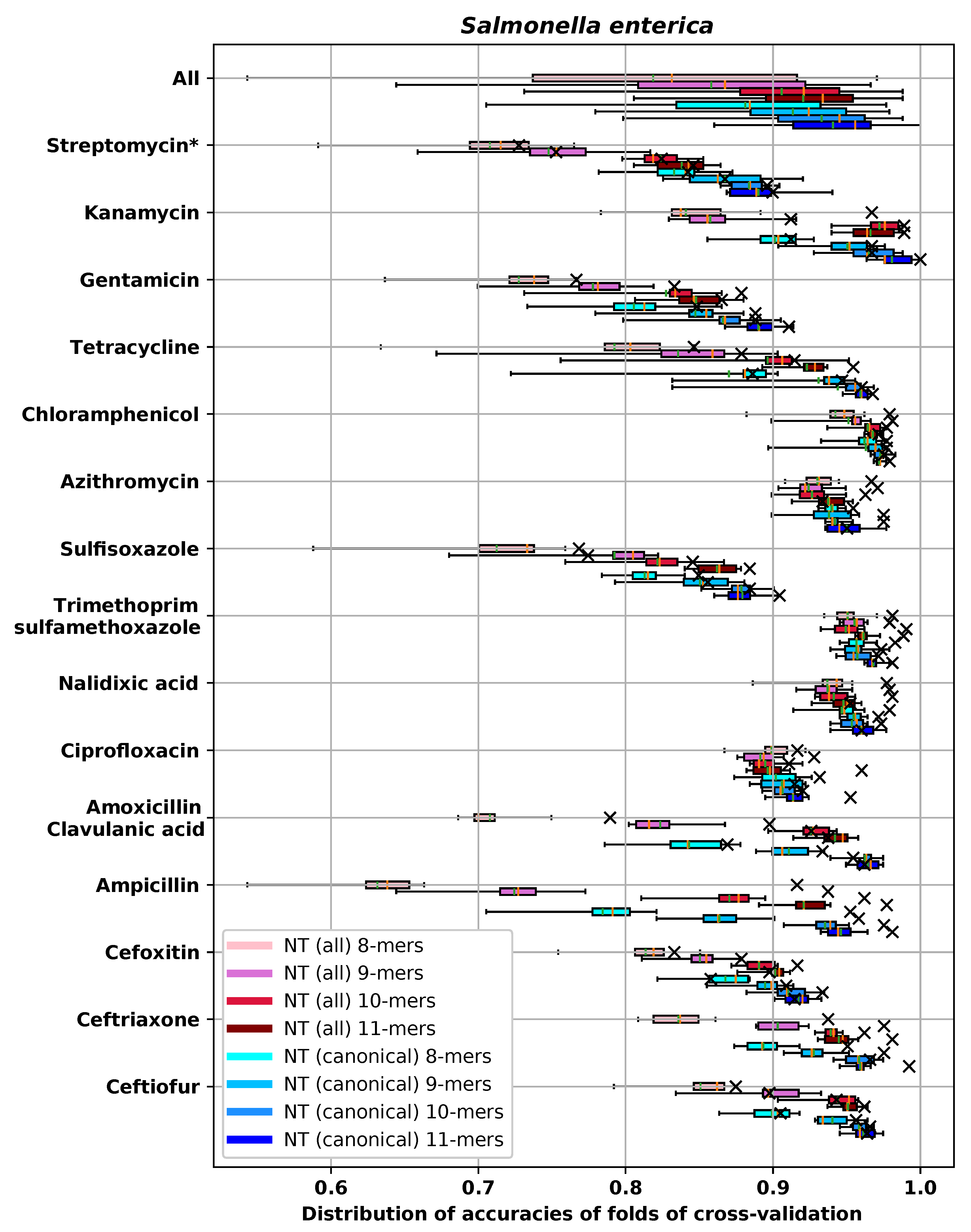
Appendix E.4. S. enterica
| RMSE-CV | RMSE-H | DD1-CV | DD1-H | DD2-CV | DD2-H | ME-CV | ME-H | VME-CV | VME-H | |
|---|---|---|---|---|---|---|---|---|---|---|
| NT 8-mers | 0.961 (0.097) | 0.881 | 0.843 (0.026) | 0.869 | 0.943 (0.015) | 0.949 | 0.002 (0.002) | 0.000 | 0.013 (0.005) | 0.009 |
| NT 9-mers | 0.768 (0.106) | 0.694 | 0.911 (0.015) | 0.934 | 0.97 (0.006) | 0.975 | 0.002 (0.002) | 0.000 | 0.008 (0.004) | 0.006 |
| NT 10-mers | 0.626 (0.106) | 0.73 | 0.962 (0.009) | 0.954 | 0.984 (0.007) | 0.983 | 0.001 (0.002) | 0.006 | 0.004 (0.004) | 0.006 |
| NT 11-mers | 0.608 (0.135) | 0.625 | 0.964 (0.008) | 0.962 | 0.986 (0.007) | 0.985 | 0.002 (0.002) | 0.000 | 0.003 (0.003) | 0.006 |
| AA 3-mers | 1.01 (0.083) | 0.902 | 0.813 (0.021) | 0.85 | 0.935 (0.013) | 0.958 | 0.002 (0.002) | 0.000 | 0.013 (0.006) | 0.011 |
| AA 4-mers | 0.65 (0.136) | 0.615 | 0.957 (0.015) | 0.958 | 0.984 (0.009) | 0.981 | 0.002 (0.002) | 0.000 | 0.003 (0.003) | 0.004 |
| AA 5-mers | 0.643 (0.129) | 0.563 | 0.967 (0.009) | 0.962 | 0.984 (0.007) | 0.987 | 0.003 (0.002) | 0.000 | 0.004 (0.003) | 0.004 |
| Gene content | 0.634 (0.132) | 0.509 | 0.958 (0.01) | 0.981 | 0.984 (0.007) | 0.994 | 0.002 (0.002) | 0.002 | 0.004 (0.002) | 0.002 |
| SNP | 1.449 (0.081) | 1.37 | 0.763 (0.022) | 0.772 | 0.877 (0.017) | 0.879 | 0.003 (0.002) | 0.002 | 0.055 (0.011) | 0.036 |
| Gene + SNP | 0.627 (0.115) | 0.693 | 0.955 (0.012) | 0.956 | 0.985 (0.005) | 0.977 | 0.002 (0.002) | 0.000 | 0.003 (0.003) | 0.008 |
| RMSE-CV | RMSE-H | DD1-CV | DD1-H | DD2-CV | DD2-H | ME-CV | ME-H | VME-CV | VME-H | |
|---|---|---|---|---|---|---|---|---|---|---|
| NT 8-mers | 1.25 (0.094) | 0.577 | 0.784 (0.03) | 0.952 | 0.906 (0.022) | 0.983 | 0.003 (0.003) | 0.000 | 0.031 (0.01) | 0.004 |
| NT 9-mers | 1.009 (0.096) | 0.665 | 0.864 (0.021) | 0.958 | 0.942 (0.011) | 0.977 | 0.003 (0.003) | 0.000 | 0.016 (0.006) | 0.01 |
| NT 10-mers | 0.817 (0.111) | 0.456 | 0.935 (0.012) | 0.975 | 0.976 (0.005) | 0.989 | 0.003 (0.003) | 0.002 | 0.011 (0.006) | 0.002 |
| NT 11-mers | 0.763 (0.097) | 0.593 | 0.946 (0.011) | 0.981 | 0.98 (0.004) | 0.99 | 0.004 (0.002) | 0.002 | 0.008 (0.005) | 0.006 |
| AA 3-mers | 1.32 (0.122) | 0.906 | 0.747 (0.038) | 0.838 | 0.892 (0.022) | 0.952 | 0.004 (0.003) | 0.000 | 0.036 (0.013) | 0.01 |
| AA 4-mers | 0.824 (0.114) | 0.669 | 0.941 (0.012) | 0.964 | 0.975 (0.01) | 0.979 | 0.005 (0.002) | 0.000 | 0.01 (0.005) | 0.01 |
| AA 5-mers | 0.758 (0.116) | 0.526 | 0.959 (0.008) | 0.981 | 0.983 (0.006) | 0.99 | 0.005 (0.003) | 0.000 | 0.008 (0.005) | 0.004 |
| Gene content | 0.787 (0.1) | 0.484 | 0.948 (0.007) | 0.981 | 0.979 (0.006) | 0.992 | 0.004 (0.002) | 0.000 | 0.01 (0.005) | 0.006 |
| SNP | 1.532 (0.073) | 1.079 | 0.76 (0.025) | 0.854 | 0.875 (0.02) | 0.93 | 0.004 (0.003) | 0.000 | 0.06 (0.009) | 0.034 |
| Gene + SNP | 0.762 (0.086) | 0.583 | 0.953 (0.007) | 0.966 | 0.979 (0.006) | 0.989 | 0.003 (0.002) | 0.002 | 0.01 (0.004) | 0.006 |
| RMSE-CV | RMSE-H | DD1-CV | DD1-H | DD2-CV | DD2-H | ME-CV | ME-H | VME-CV | VME-H | |
|---|---|---|---|---|---|---|---|---|---|---|
| NT 8-mers | 0.527 (0.025) | 0.454 | 0.94 (0.005) | 0.954 | 0.996 (0.004) | 1.000 | 0.0 (0.0) | 0.0 | 0.003 (0.002) | 0.000 |
| NT 9-mers | 0.532 (0.032) | 0.406 | 0.938 (0.018) | 0.975 | 0.996 (0.003) | 1.000 | 0.0 (0.0) | 0.0 | 0.003 (0.002) | 0.000 |
| NT 10-mers | 0.526 (0.025) | 0.404 | 0.942 (0.006) | 0.975 | 0.998 (0.002) | 0.996 | 0.0 (0.0) | 0.0 | 0.003 (0.002) | 0.000 |
| NT 11-mers | 0.509 (0.028) | 0.516 | 0.95 (0.014) | 0.950 | 0.997 (0.002) | 1.000 | 0.0 (0.0) | 0.0 | 0.003 (0.002) | 0.000 |
| AA 3-mers | 0.531 (0.03) | 0.447 | 0.933 (0.013) | 0.979 | 0.996 (0.003) | 1.000 | 0.0 (0.0) | 0.0 | 0.003 (0.002) | 0.004 |
| AA 4-mers | 0.514 (0.03) | 0.405 | 0.943 (0.013) | 0.983 | 0.998 (0.003) | 1.000 | 0.0 (0.0) | 0.0 | 0.003 (0.002) | 0.000 |
| AA 5-mers | 0.506 (0.035) | 0.471 | 0.95 (0.011) | 0.950 | 0.998 (0.002) | 1.000 | 0.0 (0.0) | 0.0 | 0.003 (0.002) | 0.004 |
| Gene content | 0.51 (0.032) | 0.388 | 0.941 (0.009) | 0.983 | 0.999 (0.002) | 0.996 | 0.0 (0.0) | 0.0 | 0.001 (0.002) | 0.000 |
| SNP | 0.521 (0.03) | 0.424 | 0.943 (0.016) | 0.967 | 0.996 (0.003) | 1.000 | 0.0 (0.0) | 0.0 | 0.003 (0.002) | 0.000 |
| Gene + SNP | 0.522 (0.027) | 0.356 | 0.94 (0.015) | 0.983 | 0.996 (0.003) | 1.000 | 0.0 (0.0) | 0.0 | 0.003 (0.002) | 0.000 |
| RMSE-CV | RMSE-H | DD1-CV | DD1-H | DD2-CV | DD2-H | ME-CV | ME-H | VME-CV | VME-H | |
|---|---|---|---|---|---|---|---|---|---|---|
| NT 8-mers | 0.774 (0.045) | 0.831 | 0.868 (0.019) | 0.858 | 0.975 (0.008) | 0.97 | 0.001 (0.001) | 0.004 | 0.011 (0.004) | 0.009 |
| NT 9-mers | 0.684 (0.048) | 0.63 | 0.895 (0.015) | 0.909 | 0.985 (0.007) | 0.994 | 0.001 (0.001) | 0.004 | 0.005 (0.003) | 0.000 |
| NT 10-mers | 0.65 (0.067) | 0.528 | 0.91 (0.015) | 0.934 | 0.989 (0.007) | 0.998 | 0.002 (0.002) | 0.000 | 0.004 (0.003) | 0.000 |
| NT 11-mers | 0.629 (0.051) | 0.597 | 0.917 (0.01) | 0.915 | 0.99 (0.004) | 0.994 | 0.001 (0.001) | 0.002 | 0.004 (0.003) | 0.000 |
| AA 3-mers | 0.765 (0.046) | 0.793 | 0.865 (0.017) | 0.879 | 0.976 (0.005) | 0.968 | 0.001 (0.002) | 0.002 | 0.007 (0.003) | 0.011 |
| AA 4-mers | 0.617 (0.052) | 0.77 | 0.919 (0.013) | 0.92 | 0.992 (0.005) | 0.979 | 0.001 (0.001) | 0.008 | 0.003 (0.003) | 0.008 |
| AA 5-mers | 0.621 (0.061) | 0.622 | 0.926 (0.006) | 0.919 | 0.99 (0.005) | 0.996 | 0.002 (0.002) | 0.004 | 0.004 (0.003) | 0.000 |
| Gene content | 0.624 (0.037) | 0.58 | 0.924 (0.01) | 0.909 | 0.99 (0.005) | 0.992 | 0.002 (0.001) | 0.000 | 0.004 (0.003) | 0.002 |
| SNP | 1.163 (0.058) | 1.211 | 0.768 (0.013) | 0.765 | 0.915 (0.014) | 0.907 | 0.001 (0.001) | 0.004 | 0.045 (0.012) | 0.038 |
| Gene + SNP | 0.622 (0.046) | 0.621 | 0.923 (0.009) | 0.911 | 0.991 (0.005) | 0.987 | 0.001 (0.001) | 0.002 | 0.004 (0.003) | 0.002 |
| RMSE-CV | RMSE-H | DD1-CV | DD1-H | DD2-CV | DD2-H | ME-CV | ME-H | VME-CV | VME-H | |
|---|---|---|---|---|---|---|---|---|---|---|
| NT 8-mers | 0.724 (0.079) | 0.739 | 0.899 (0.016) | 0.905 | 0.974 (0.012) | 0.975 | 0.001 (0.001) | 0.004 | 0.01 (0.006) | 0.009 |
| NT 9-mers | 0.61 (0.053) | 0.574 | 0.94 (0.013) | 0.956 | 0.988 (0.007) | 0.992 | 0.002 (0.002) | 0.004 | 0.004 (0.002) | 0.004 |
| NT 10-mers | 0.573 (0.053) | 0.452 | 0.958 (0.006) | 0.966 | 0.992 (0.004) | 1.0 | 0.002 (0.002) | 0.000 | 0.005 (0.003) | 0.0 |
| NT 11-mers | 0.548 (0.053) | 0.522 | 0.961 (0.009) | 0.964 | 0.993 (0.004) | 0.994 | 0.002 (0.002) | 0.004 | 0.004 (0.003) | 0.002 |
| AA 3-mers | 0.71 (0.075) | 0.7 | 0.897 (0.021) | 0.892 | 0.977 (0.009) | 0.983 | 0.002 (0.002) | 0.000 | 0.007 (0.004) | 0.008 |
| AA 4-mers | 0.56 (0.065) | 0.583 | 0.96 (0.006) | 0.954 | 0.992 (0.005) | 0.992 | 0.002 (0.003) | 0.002 | 0.005 (0.003) | 0.006 |
| AA 5-mers | 0.546 (0.057) | 0.553 | 0.965 (0.008) | 0.975 | 0.993 (0.004) | 0.992 | 0.003 (0.003) | 0.000 | 0.004 (0.003) | 0.008 |
| Gene content | 0.553 (0.051) | 0.537 | 0.961 (0.005) | 0.964 | 0.993 (0.005) | 0.994 | 0.002 (0.002) | 0.002 | 0.005 (0.003) | 0.004 |
| SNP | 1.161 (0.058) | 1.147 | 0.777 (0.014) | 0.789 | 0.909 (0.014) | 0.911 | 0.003 (0.003) | 0.000 | 0.042 (0.011) | 0.047 |
| Gene + SNP | 0.549 (0.051) | 0.646 | 0.958 (0.007) | 0.954 | 0.993 (0.003) | 0.985 | 0.001 (0.001) | 0.006 | 0.004 (0.003) | 0.008 |
| RMSE-CV | RMSE-H | DD1-CV | DD1-H | DD2-CV | DD2-H | ME-CV | ME-H | VME-CV | VME-H | |
|---|---|---|---|---|---|---|---|---|---|---|
| NT 8-mers | 0.965 (0.141) | 0.615 | 0.893 (0.014) | 0.951 | 0.953 (0.011) | 0.979 | 0.004 (0.003) | 0.002 | 0.012 (0.007) | 0.004 |
| NT 9-mers | 0.782 (0.107) | 0.408 | 0.928 (0.012) | 0.975 | 0.975 (0.007) | 0.994 | 0.003 (0.002) | 0.000 | 0.007 (0.003) | 0.002 |
| NT 10-mers | 0.647 (0.122) | 0.541 | 0.958 (0.011) | 0.966 | 0.986 (0.006) | 0.989 | 0.003 (0.002) | 0.002 | 0.006 (0.004) | 0.004 |
| NT 11-mers | 0.671 (0.132) | 0.292 | 0.959 (0.006) | 0.992 | 0.986 (0.005) | 0.998 | 0.003 (0.003) | 0.000 | 0.006 (0.003) | 0.002 |
| AA 3-mers | 0.919 (0.077) | 0.674 | 0.891 (0.016) | 0.951 | 0.957 (0.007) | 0.975 | 0.004 (0.002) | 0.002 | 0.009 (0.003) | 0.004 |
| AA 4-mers | 0.66 (0.12) | 0.531 | 0.954 (0.006) | 0.968 | 0.985 (0.005) | 0.989 | 0.003 (0.002) | 0.002 | 0.006 (0.004) | 0.004 |
| AA 5-mers | 0.673 (0.123) | 0.292 | 0.963 (0.009) | 0.987 | 0.986 (0.005) | 0.994 | 0.003 (0.003) | 0.000 | 0.006 (0.003) | 0.000 |
| Gene content | 0.644 (0.1) | 0.402 | 0.961 (0.008) | 0.979 | 0.987 (0.004) | 0.994 | 0.002 (0.002) | 0.002 | 0.006 (0.003) | 0.000 |
| SNP | 1.588 (0.098) | 1.580 | 0.78 (0.021) | 0.808 | 0.875 (0.016) | 0.89 | 0.006 (0.004) | 0.006 | 0.046 (0.009) | 0.051 |
| Gene + SNP | 0.648 (0.133) | 0.700 | 0.955 (0.008) | 0.96 | 0.985 (0.006) | 0.979 | 0.003 (0.002) | 0.000 | 0.006 (0.004) | 0.011 |
| RMSE-CV | RMSE-H | DD1-CV | DD1-H | DD2-CV | DD2-H | ME-CV | ME-H | VME-CV | VME-H | |
|---|---|---|---|---|---|---|---|---|---|---|
| NT 8-mers | 0.495 (0.035) | 0.437 | 0.962 (0.012) | 0.977 | 0.994 (0.002) | 1.000 | 0.001 (0.001) | 0.000 | 0.001 (0.001) | 0.000 |
| NT 9-mers | 0.473 (0.03) | 0.45 | 0.963 (0.022) | 0.977 | 0.995 (0.002) | 0.998 | 0.001 (0.001) | 0.002 | 0.001 (0.001) | 0.000 |
| NT 10-mers | 0.456 (0.025) | 0.436 | 0.973 (0.005) | 0.975 | 0.997 (0.001) | 0.998 | 0.0 (0.001) | 0.000 | 0.001 (0.001) | 0.000 |
| NT 11-mers | 0.45 (0.019) | 0.413 | 0.972 (0.002) | 0.979 | 0.997 (0.002) | 1.000 | 0.0 (0.001) | 0.000 | 0.001 (0.001) | 0.000 |
| AA 3-mers | 0.507 (0.045) | 0.449 | 0.958 (0.01) | 0.979 | 0.993 (0.003) | 1.000 | 0.0 (0.001) | 0.000 | 0.002 (0.002) | 0.000 |
| AA 4-mers | 0.459 (0.029) | 0.445 | 0.967 (0.016) | 0.991 | 0.997 (0.002) | 0.998 | 0.0 (0.001) | 0.002 | 0.001 (0.002) | 0.000 |
| AA 5-mers | 0.435 (0.023) | 0.423 | 0.979 (0.005) | 0.977 | 0.998 (0.002) | 0.998 | 0.0 (0.001) | 0.000 | 0.001 (0.001) | 0.002 |
| Gene content | 0.443 (0.028) | 0.427 | 0.977 (0.005) | 0.985 | 0.998 (0.002) | 0.996 | 0.0 (0.0) | 0.002 | 0.001 (0.002) | 0.002 |
| SNP | 0.521 (0.048) | 0.486 | 0.956 (0.024) | 0.97 | 0.99 (0.003) | 0.994 | 0.002 (0.003) | 0.000 | 0.002 (0.002) | 0.002 |
| Gene + SNP | 0.446 (0.025) | 0.449 | 0.978 (0.005) | 0.975 | 0.997 (0.002) | 0.998 | 0.0 (0.001) | 0.000 | 0.001 (0.001) | 0.002 |
| RMSE-CV | RMSE-H | DD1-CV | DD1-H | DD2-CV | DD2-H | ME-CV | ME-H | VME-CV | VME-H | |
|---|---|---|---|---|---|---|---|---|---|---|
| NT 8-mers | 0.64 (0.048) | 0.54 | 0.902 (0.016) | 0.932 | 0.987 (0.004) | 0.991 | 0.0 (0.0) | 0.0 | 0.0 (0.001) | 0.0 |
| NT 9-mers | 0.628 (0.045) | 0.58 | 0.906 (0.015) | 0.915 | 0.987 (0.005) | 0.991 | 0.0 (0.0) | 0.0 | 0.001 (0.001) | 0.0 |
| NT 10-mers | 0.604 (0.039) | 0.51 | 0.907 (0.009) | 0.92 | 0.989 (0.003) | 0.992 | 0.0 (0.0) | 0.0 | 0.001 (0.001) | 0.0 |
| NT 11-mers | 0.561 (0.034) | 0.458 | 0.913 (0.008) | 0.953 | 0.991 (0.003) | 0.994 | 0.0 (0.0) | 0.0 | 0.0 (0.001) | 0.0 |
| AA 3-mers | 0.65 (0.035) | 0.585 | 0.903 (0.014) | 0.901 | 0.987 (0.003) | 0.991 | 0.0 (0.001) | 0.0 | 0.0 (0.001) | 0.0 |
| AA 4-mers | 0.617 (0.038) | 0.489 | 0.906 (0.014) | 0.922 | 0.987 (0.003) | 0.996 | 0.0 (0.0) | 0.0 | 0.0 (0.001) | 0.0 |
| AA 5-mers | 0.541 (0.036) | 0.437 | 0.921 (0.012) | 0.947 | 0.992 (0.003) | 0.998 | 0.0 (0.0) | 0.0 | 0.0 (0.0) | 0.0 |
| Gene content | 0.618 (0.061) | 0.517 | 0.904 (0.01) | 0.935 | 0.987 (0.004) | 0.994 | 0.0 (0.0) | 0.0 | 0.0 (0.0) | 0.0 |
| SNP | 0.611 (0.036) | 0.542 | 0.909 (0.017) | 0.937 | 0.989 (0.004) | 0.992 | 0.0 (0.0) | 0.0 | 0.001 (0.001) | 0.0 |
| Gene + SNP | 0.572 (0.057) | 0.495 | 0.91 (0.015) | 0.956 | 0.99 (0.004) | 0.992 | 0.0 (0.0) | 0.0 | 0.0 (0.0) | 0.0 |
| RMSE-CV | RMSE-H | DD1-CV | DD1-H | DD2-CV | DD2-H | ME-CV | ME-H | VME-CV | VME-H | |
|---|---|---|---|---|---|---|---|---|---|---|
| NT 8-mers | 1.123 (0.097) | 0.978 | 0.806 (0.033) | 0.848 | 0.932 (0.016) | 0.956 | 0.001 (0.001) | 0.002 | 0.024 (0.008) | 0.006 |
| NT 9-mers | 0.989 (0.083) | 0.77 | 0.847 (0.026) | 0.888 | 0.958 (0.009) | 0.985 | 0.002 (0.002) | 0.002 | 0.014 (0.007) | 0.002 |
| NT 10-mers | 0.901 (0.077) | 0.846 | 0.866 (0.026) | 0.888 | 0.97 (0.01) | 0.968 | 0.002 (0.002) | 0.0 | 0.011 (0.004) | 0.006 |
| NT 11-mers | 0.787 (0.063) | 0.972 | 0.89 (0.014) | 0.911 | 0.981 (0.006) | 0.975 | 0.001 (0.001) | 0.004 | 0.005 (0.003) | 0.011 |
| AA 3-mers | 1.172 (0.108) | 0.94 | 0.791 (0.033) | 0.843 | 0.928 (0.018) | 0.962 | 0.002 (0.002) | 0.008 | 0.026 (0.009) | 0.004 |
| AA 4-mers | 0.866 (0.085) | 0.773 | 0.88 (0.017) | 0.898 | 0.975 (0.008) | 0.981 | 0.002 (0.001) | 0.002 | 0.009 (0.003) | 0.000 |
| AA 5-mers | 0.797 (0.051) | 0.745 | 0.895 (0.013) | 0.905 | 0.983 (0.004) | 0.991 | 0.002 (0.002) | 0.002 | 0.005 (0.003) | 0.004 |
| Gene content | 0.81 (0.06) | 0.766 | 0.892 (0.015) | 0.926 | 0.981 (0.005) | 0.989 | 0.001 (0.001) | 0.004 | 0.006 (0.003) | 0.000 |
| SNP | 1.093 (0.088) | 1.057 | 0.843 (0.021) | 0.865 | 0.952 (0.009) | 0.964 | 0.005 (0.005) | 0.006 | 0.018 (0.005) | 0.013 |
| Gene + SNP | 0.795 (0.055) | 0.914 | 0.889 (0.017) | 0.89 | 0.982 (0.005) | 0.972 | 0.001 (0.001) | 0.004 | 0.005 (0.003) | 0.011 |
| RMSE-CV | RMSE-H | DD1-CV | DD1-H | DD2-CV | DD2-H | ME-CV | ME-H | VME-CV | VME-H | |
|---|---|---|---|---|---|---|---|---|---|---|
| NT 8-mers | 0.788 (0.155) | 0.714 | 0.901 (0.021) | 0.912 | 0.957 (0.024) | 0.956 | 0.005 (0.006) | 0.000 | 0.023 (0.017) | 0.022 |
| NT 9-mers | 0.525 (0.167) | 0.484 | 0.951 (0.02) | 0.967 | 0.981 (0.016) | 0.978 | 0.0 (0.0) | 0.000 | 0.011 (0.014) | 0.011 |
| NT 10-mers | 0.423 (0.148) | 0.345 | 0.965 (0.018) | 0.967 | 0.989 (0.008) | 1.000 | 0.0 (0.0) | 0.000 | 0.006 (0.008) | 0.000 |
| NT 11-mers | 0.401 (0.188) | 0.155 | 0.981 (0.013) | 1.000 | 0.988 (0.011) | 1.000 | 0.001 (0.004) | 0.000 | 0.01 (0.012) | 0.000 |
| AA 3-mers | 0.641 (0.157) | 0.554 | 0.932 (0.024) | 0.945 | 0.97 (0.021) | 0.978 | 0.002 (0.005) | 0.000 | 0.014 (0.014) | 0.022 |
| AA 4-mers | 0.458 (0.102) | 0.393 | 0.972 (0.013) | 0.989 | 0.985 (0.007) | 0.989 | 0.001 (0.004) | 0.000 | 0.008 (0.006) | 0.011 |
| AA 5-mers | 0.321 (0.179) | 0.15 | 0.986 (0.013) | 0.989 | 0.993 (0.01) | 1.000 | 0.0 (0.0) | 0.000 | 0.006 (0.008) | 0.000 |
| Gene content | 0.402 (0.14) | 0.126 | 0.98 (0.019) | 1.000 | 0.99 (0.009) | 1.000 | 0.0 (0.0) | 0.000 | 0.007 (0.008) | 0.000 |
| SNP | 0.788 (0.175) | 0.752 | 0.914 (0.022) | 0.912 | 0.953 (0.021) | 0.945 | 0.006 (0.008) | 0.011 | 0.028 (0.026) | 0.011 |
| Gene + SNP | 0.503 (0.086) | 0.256 | 0.943 (0.025) | 0.978 | 0.987 (0.01) | 1.000 | 0.0 (0.0) | 0.000 | 0.007 (0.01) | 0.000 |
| RMSE-CV | RMSE-H | DD1-CV | DD1-H | DD2-CV | DD2-H | ME-CV | ME-H | VME-CV | VME-H | |
|---|---|---|---|---|---|---|---|---|---|---|
| NT 8-mers | 0.556 (0.026) | 0.394 | 0.947 (0.013) | 0.979 | 0.99 (0.003) | 1.000 | 0.0 (0.0) | 0.0 | 0.007 (0.003) | 0.000 |
| NT 9-mers | 0.546 (0.023) | 0.498 | 0.955 (0.006) | 0.972 | 0.991 (0.002) | 0.994 | 0.0 (0.001) | 0.0 | 0.007 (0.002) | 0.006 |
| NT 10-mers | 0.511 (0.023) | 0.434 | 0.953 (0.009) | 0.973 | 0.993 (0.002) | 0.998 | 0.0 (0.0) | 0.0 | 0.005 (0.002) | 0.002 |
| NT 11-mers | 0.475 (0.036) | 0.452 | 0.96 (0.011) | 0.96 | 0.996 (0.003) | 1.000 | 0.0 (0.001) | 0.0 | 0.002 (0.001) | 0.000 |
| AA 3-mers | 0.559 (0.035) | 0.512 | 0.945 (0.019) | 0.972 | 0.99 (0.002) | 0.991 | 0.0 (0.0) | 0.0 | 0.007 (0.002) | 0.008 |
| AA 4-mers | 0.523 (0.037) | 0.454 | 0.957 (0.006) | 0.97 | 0.994 (0.004) | 0.992 | 0.0 (0.0) | 0.0 | 0.005 (0.003) | 0.004 |
| AA 5-mers | 0.475 (0.031) | 0.431 | 0.961 (0.008) | 0.973 | 0.995 (0.003) | 1.000 | 0.0 (0.0) | 0.0 | 0.003 (0.002) | 0.000 |
| Gene content | 0.539 (0.03) | 0.429 | 0.953 (0.005) | 0.973 | 0.992 (0.004) | 0.994 | 0.0 (0.0) | 0.0 | 0.007 (0.002) | 0.004 |
| SNP | 0.535 (0.044) | 0.438 | 0.954 (0.007) | 0.973 | 0.99 (0.003) | 0.998 | 0.0 (0.0) | 0.0 | 0.006 (0.002) | 0.000 |
| Gene + SNP | 0.513 (0.036) | 0.501 | 0.958 (0.005) | 0.964 | 0.995 (0.002) | 0.994 | 0.0 (0.0) | 0.0 | 0.005 (0.003) | 0.002 |
| RMSE-CV | RMSE-H | DD1-CV | DD1-H | DD2-CV | DD2-H | ME-CV | ME-H | VME-CV | VME-H | |
|---|---|---|---|---|---|---|---|---|---|---|
| NT 8-mers | 0.87 (0.064) | 0.835 | 0.833 (0.028) | 0.842 | 0.956 (0.01) | 0.971 | 0.02 (0.011) | 0.022 | 0.021 (0.012) | 0.025 |
| NT 9-mers | 0.77 (0.074) | 0.731 | 0.867 (0.03) | 0.867 | 0.972 (0.012) | 0.978 | 0.012 (0.007) | 0.018 | 0.021 (0.013) | 0.022 |
| NT 10-mers | 0.742 (0.052) | 0.723 | 0.884 (0.014) | 0.896 | 0.975 (0.009) | 0.968 | 0.01 (0.006) | 0.014 | 0.023 (0.01) | 0.025 |
| NT 11-mers | 0.731 (0.073) | 0.692 | 0.89 (0.021) | 0.9 | 0.976 (0.012) | 0.975 | 0.008 (0.005) | 0.011 | 0.021 (0.012) | 0.039 |
| AA 3-mers | 0.891 (0.077) | 0.824 | 0.811 (0.032) | 0.832 | 0.953 (0.017) | 0.961 | 0.022 (0.016) | 0.018 | 0.023 (0.014) | 0.011 |
| AA 4-mers | 0.741 (0.097) | 0.712 | 0.89 (0.034) | 0.889 | 0.974 (0.014) | 0.975 | 0.009 (0.008) | 0.004 | 0.026 (0.016) | 0.029 |
| AA 5-mers | 0.721 (0.072) | 0.724 | 0.891 (0.014) | 0.896 | 0.974 (0.011) | 0.975 | 0.008 (0.005) | 0.007 | 0.026 (0.01) | 0.025 |
| Gene content | 0.724 (0.078) | 0.7 | 0.894 (0.024) | 0.918 | 0.978 (0.01) | 0.982 | 0.008 (0.005) | 0.007 | 0.025 (0.015) | 0.029 |
| SNP | 0.754 (0.06) | 0.749 | 0.873 (0.019) | 0.878 | 0.973 (0.01) | 0.978 | 0.013 (0.007) | 0.007 | 0.014 (0.012) | 0.025 |
| Gene + SNP | 0.723 (0.047) | 0.778 | 0.886 (0.013) | 0.875 | 0.977 (0.008) | 0.971 | 0.007 (0.005) | 0.007 | 0.019 (0.013) | 0.036 |
| RMSE-CV | RMSE-H | DD1-CV | DD1-H | DD2-CV | DD2-H | ME-CV | ME-H | VME-CV | VME-H | |
|---|---|---|---|---|---|---|---|---|---|---|
| NT 8-mers | 0.896 (0.053) | 0.812 | 0.813 (0.014) | 0.85 | 0.954 (0.014) | 0.963 | 0.001 (0.002) | 0.000 | 0.051 (0.015) | 0.020 |
| NT 9-mers | 0.798 (0.063) | 0.713 | 0.85 (0.025) | 0.856 | 0.971 (0.01) | 0.982 | 0.001 (0.001) | 0.002 | 0.032 (0.014) | 0.014 |
| NT 10-mers | 0.741 (0.051) | 0.69 | 0.879 (0.014) | 0.884 | 0.978 (0.009) | 0.982 | 0.0 (0.001) | 0.000 | 0.018 (0.007) | 0.012 |
| NT 11-mers | 0.721 (0.047) | 0.702 | 0.879 (0.013) | 0.904 | 0.98 (0.005) | 0.978 | 0.001 (0.001) | 0.000 | 0.014 (0.005) | 0.012 |
| AA 3-mers | 0.951 (0.081) | 0.869 | 0.792 (0.027) | 0.791 | 0.945 (0.014) | 0.972 | 0.001 (0.002) | 0.002 | 0.063 (0.02) | 0.028 |
| AA 4-mers | 0.738 (0.031) | 0.826 | 0.87 (0.015) | 0.856 | 0.979 (0.007) | 0.97 | 0.0 (0.001) | 0.002 | 0.019 (0.004) | 0.010 |
| AA 5-mers | 0.713 (0.035) | 0.736 | 0.888 (0.009) | 0.88 | 0.982 (0.004) | 0.976 | 0.001 (0.001) | 0.000 | 0.011 (0.006) | 0.014 |
| Gene content | 0.715 (0.044) | 0.712 | 0.885 (0.009) | 0.878 | 0.983 (0.006) | 0.986 | 0.0 (0.0) | 0.000 | 0.014 (0.003) | 0.010 |
| SNP | 0.805 (0.055) | 0.739 | 0.864 (0.013) | 0.874 | 0.971 (0.007) | 0.976 | 0.001 (0.001) | 0.000 | 0.021 (0.008) | 0.016 |
| Gene + SNP | 0.721 (0.041) | 0.71 | 0.879 (0.013) | 0.886 | 0.982 (0.005) | 0.98 | 0.0 (0.001) | 0.004 | 0.015 (0.006) | 0.014 |
| RMSE-CV | RMSE-H | DD1-CV | DD1-H | DD2-CV | DD2-H | ME-CV | ME-H | VME-CV | VME-H | |
|---|---|---|---|---|---|---|---|---|---|---|
| NT 8-mers | 0.821 (0.135) | 0.699 | 0.87 (0.051) | 0.886 | 0.948 (0.027) | 0.968 | 0.023 (0.015) | 0.019 | 0.001 (0.001) | 0.000 |
| NT 9-mers | 0.647 (0.1) | 0.665 | 0.931 (0.034) | 0.947 | 0.972 (0.012) | 0.973 | 0.012 (0.007) | 0.017 | 0.001 (0.002) | 0.000 |
| NT 10-mers | 0.592 (0.087) | 0.556 | 0.944 (0.038) | 0.96 | 0.979 (0.006) | 0.983 | 0.007 (0.004) | 0.009 | 0.001 (0.001) | 0.000 |
| NT 11-mers | 0.563 (0.061) | 0.48 | 0.959 (0.006) | 0.968 | 0.982 (0.006) | 0.989 | 0.007 (0.003) | 0.002 | 0.001 (0.002) | 0.000 |
| AA 3-mers | 0.802 (0.111) | 0.81 | 0.865 (0.052) | 0.869 | 0.957 (0.016) | 0.954 | 0.02 (0.009) | 0.03 | 0.003 (0.003) | 0.000 |
| AA 4-mers | 0.562 (0.07) | 0.548 | 0.962 (0.014) | 0.958 | 0.982 (0.005) | 0.985 | 0.008 (0.002) | 0.006 | 0.001 (0.001) | 0.000 |
| AA 5-mers | 0.545 (0.076) | 0.402 | 0.969 (0.008) | 0.985 | 0.982 (0.006) | 0.992 | 0.007 (0.004) | 0.004 | 0.0 (0.001) | 0.000 |
| Gene content | 0.509 (0.081) | 0.604 | 0.973 (0.01) | 0.968 | 0.985 (0.006) | 0.979 | 0.005 (0.002) | 0.015 | 0.0 (0.0) | 0.000 |
| SNP | 0.869 (0.13) | 0.768 | 0.882 (0.051) | 0.899 | 0.941 (0.027) | 0.956 | 0.028 (0.019) | 0.015 | 0.001 (0.001) | 0.002 |
| Gene + SNP | 0.539 (0.066) | 0.597 | 0.963 (0.024) | 0.97 | 0.984 (0.006) | 0.979 | 0.006 (0.003) | 0.009 | 0.001 (0.001) | 0.000 |
| RMSE-CV | RMSE-H | DD1-CV | DD1-H | DD2-CV | DD2-H | ME-CV | ME-H | VME-CV | VME-H | |
|---|---|---|---|---|---|---|---|---|---|---|
| NT 8-mers | 0.578 (0.05) | 0.284 | 0.957 (0.007) | 0.983 | 0.988 (0.002) | 0.996 | 0.0 (0.001) | 0.000 | 0.008 (0.002) | 0.002 |
| NT 9-mers | 0.557 (0.083) | 0.469 | 0.957 (0.011) | 0.973 | 0.989 (0.004) | 0.994 | 0.0 (0.0) | 0.000 | 0.008 (0.003) | 0.004 |
| NT 10-mers | 0.506 (0.067) | 0.323 | 0.957 (0.01) | 0.972 | 0.989 (0.002) | 0.998 | 0.0 (0.0) | 0.000 | 0.007 (0.002) | 0.000 |
| NT 11-mers | 0.394 (0.063) | 0.327 | 0.968 (0.006) | 0.981 | 0.994 (0.003) | 0.998 | 0.001 (0.001) | 0.002 | 0.003 (0.003) | 0.000 |
| AA 3-mers | 0.573 (0.072) | 0.232 | 0.96 (0.008) | 0.987 | 0.988 (0.003) | 1.000 | 0.0 (0.001) | 0.000 | 0.009 (0.002) | 0.000 |
| AA 4-mers | 0.443 (0.077) | 0.247 | 0.964 (0.008) | 0.975 | 0.991 (0.004) | 0.998 | 0.0 (0.001) | 0.000 | 0.005 (0.003) | 0.002 |
| AA 5-mers | 0.349 (0.064) | 0.224 | 0.98 (0.005) | 0.991 | 0.996 (0.002) | 1.000 | 0.0 (0.001) | 0.000 | 0.001 (0.001) | 0.000 |
| Gene content | 0.346 (0.055) | 0.324 | 0.971 (0.01) | 0.981 | 0.996 (0.002) | 0.998 | 0.0 (0.001) | 0.000 | 0.002 (0.002) | 0.002 |
| SNP | 0.532 (0.09) | 0.364 | 0.961 (0.009) | 0.972 | 0.989 (0.003) | 0.994 | 0.0 (0.0) | 0.000 | 0.007 (0.003) | 0.006 |
| Gene + SNP | 0.436 (0.091) | 0.319 | 0.966 (0.009) | 0.972 | 0.992 (0.004) | 0.994 | 0.0 (0.0) | 0.000 | 0.005 (0.003) | 0.006 |
Appendix F. Canonical and Non-Canonical Nucleotide k-mers


Appendix G. Measuring Feature Stability in Different Methods
| Method | Score |
|---|---|
| NT 8-mers | 0.98275 |
| NT 9-mers | 0.99636 |
| NT 10-mers | 0.99919 |
| NT 11-mers | 0.99978 |
| AA 3-mers | 0.90825 |
| AA 4-mers | 0.99675 |
| AA 5-mers | 0.99973 |
| Gene content | 0.99536 |
| SNP | 0.99952 |
| Gene content + SNP | 0.99973 |
Appendix H. Performances of the Selected-Feature Model Pipelines
| Method | Average (STD Accuracy of All Feature Pipeline) | Ratio of Datasets Where Selected-Feature Pipeline Reaches a Better Accuracy | Average (STD) of Required Features to Reach a Better Accuracy |
|---|---|---|---|
| NT 8-mers | 0.8316 (0.1112) | 0.9811 | 11.3774 (9.2456) |
| NT 9-mers | 0.8545 (0.0985) | 0.9245 | 10.6604 (10.7842) |
| NT 10-mers | 0.8723 (0.0993) | 0.8679 | 14.283 (12.7817) |
| NT 11-mers | 0.8784 (0.0943) | 0.9245 | 13.4528 (12.509) |
| AA 3-mers | 0.8233 (0.116) | 0.9057 | 13.5094 (12.438) |
| AA 4-mers | 0.8716 (0.0979) | 0.9057 | 11.6038 (11.0288) |
| AA 5-mers | 0.8849 (0.0963) | 0.717 | 17.8491 (15.4607) |
| Gene content | 0.8561 (0.1258) | 0.6604 | 21.0566 (16.1986) |
| SNP | 0.8239 (0.1101) | 0.6792 | 19.7547 (16.4511) |
| Gene content + SNP | 0.8696 (0.1005) | 0.717 | 19.3962 (15.838) |
Appendix I. Resources Used for Example Datasets
| Method | Number of Features | Number of Cores | Maximum Memory Usage | Wall-Clock |
|---|---|---|---|---|
| NT 8-mers | 32,808 | 2 | 3 GB | 00:25:19 |
| NT 9-mers | 124,591 | 2 | 20 GB | 00:41:28 |
| NT 10-mers | 404,690 | 2 | 28 GB | 01:25:03 |
| NT 11-mers | 1,029,088 | 2 | 41 GB | 03:13:57 |
| AA 3-mer | 8035 | 2 | 2 GB | 00:22:47 |
| AA 4-mer | 140,093 | 2 | 25 GB | 00:53:54 |
| AA 5-mer | 935,293 | 2 | 38 GB | 03:28:11 |
| Gene content | 14,981 | 2 | 2 GB | 00:24:24 |
| SNP | 331,936 | 2 | 30 GB | 01:08:55 |
| Gene content + SNP | 346,917 | 2 | 31 GB | 00:56:31 |
| Method | Number of Features | Number of Cores | Maximum Memory Usage | Wall-Clock |
|---|---|---|---|---|
| NT 8-mers | 32,896 | 2 | 3 GB | 00:27:54 |
| NT 9-mers | 131,012 | 2 | 23 GB | 00:45:16 |
| NT 10-mers | 507,346 | 10 | 30 GB | 00:58:07 |
| NT 11-mers | 1,588,941 | 10 | 90 GB | 02:22:14 |
| AA 3-mer | 8818 | 2 | 2 GB | 00:23:38 |
| AA 4-mer | 149,817 | 2 | 25 GB | 00:37:49 |
| AA 5-mer | 1,057,709 | 5 | 54 GB | 01:37:41 |
| Gene content | 36,458 | 2 | 3 GB | 00:30:07 |
| SNP | 300,296 | 2 | 32 GB | 01:09:56 |
| Gene content + SNP | 336,754 | 2 | 33 GB | 01:18:53 |
| Method | Number of Features | Number of Cores | Maximum Memory Usage | Wall-Clock |
|---|---|---|---|---|
| NT 8-mers | 32,896 | 2 | 7 GB | 01:02:34 |
| NT 9-mers | 131,072 | 2 | 23 GB | 01:57:17 |
| NT 10-mers | 524,798 | 10 | 91 GB | 03:08:46 |
| NT 11-mers | 2,095,237 | 22 | 309 GB | 07:29:17 |
| AA 3-mer | 8091 | 2 | 2 GB | 00:46:07 |
| AA 4-mer | 159,859 | 2 | 27 GB | 01:39:31 |
| AA 5-mer | 2,463,537 | 10 | 283 GB | 06:10:21 |
| Gene content | 129,175 | 2 | 13 GB | 00:49:22 |
| SNP | 2,508,568 | 10 | 238 GB | 03:58:14 |
| Gene content + SNP | 2,637,743 | 10 | 251 GB | 04:29:25 |
| Method | Number of Features | Number of Cores | Maximum Memory Usage | Wall-Clock |
|---|---|---|---|---|
| NT 8-mers | 32,896 | 2 | 19 GB | 02:39:14 |
| NT 9-mers | 131,072 | 6 | 73 GB | 04:52:28 |
| NT 10-mers | 524,799 | 21 | 282 GB | 06:47:57 |
| NT 11-mers | 2,092,713 | 62 | 1002 GB | 22:52:44 |
| AA 3-mer | 9090 | 2 | 5 GB | 01:40:46 |
| AA 4-mer | 164,507 | 4 | 86 GB | 03:30:33 |
| AA 5-mer | 2,389,091 | 62 | 876 GB | 20:32:39 |
| Gene content | 128,290 | 4 | 39 GB | 01:56:19 |
| SNP | 2,472,276 | 10 | 739 GB | 00:51:39 |
| Gene content + SNP | 2,600,566 | 10 | 815 GB | 01:34:59 |
Appendix J. Chemical Structure of Antibiotics
| Classification | Antibiotic Name | Structure |
| Aminoglycosides | streptomycin |  |
| Aminoglycosides | amikacin |  |
| Aminoglycosides | kanamycin |  |
| Aminoglycosides | tobramycin |  |
| Aminoglycosides | spectinomycin |  |
| Aminoglycosides | gentamicin |  |
| Tetracyclines | tetracycline |  |
| Amphenicols | chloramphenicol |  |
| Amphenicols | florfenicol |  |
| Macrolides | azithromycin |  |
| Macrolides | erythromycin |  |
| Macrolides | telithromycin |  |
| Lincosamides | clindamycin |  |
| Antifolates | trimethoprim |  |
| Antifolates | sulfisoxazole |  |
| Quinolones | nalidixic acid |  |
| Quinolones | ciprofloxacin |  |
| Quinolones | levofloxacin |  |
| Nitrofurans | nitrofurantoin |  |
| Penicillins | penicillin |  |
| Penicillins | amoxicillin |  |
| Penicillins | ampicillin |  |
| Penicillins | piperacillin |  |
| Carbapenems | imipenem |  |
| Carbapenems | meropenem |  |
| Cephalosporins/Cephamycins | cefazolin |  |
| Cephalosporins/Cephamycins | ceftriaxone |  |
| Cephalosporins/Cephamycins | cefepime |  |
| Cephalosporins/Cephamycins | cefoxitin |  |
| Cephalosporins/Cephamycins | cefixime |  |
| Cephalosporins/Cephamycins | ceftazidime/clavulanic acid |  |
| Cephalosporins/Cephamycins | cefpodoxime proxetil |  |
| Cephalosporins/Cephamycins | ceftiofur |  |
| Monobactams | aztreonam |  |
References
- Cassini, A.; Högberg, L.D.; Plachouras, D.; Quattrocchi, A.; Hoxha, A.; Simonsen, G.S.; Colomb-Cotinat, M.; Kretzschmar, M.E.; Devleesschauwer, B.; Cecchini, M.; et al. Attributable deaths and disability-adjusted life-years caused by infections with antibiotic-resistant bacteria in the EU and the European Economic Area in 2015: A population-level modelling analysis. Lancet Infect. Dis. 2019, 19, 56–66. [Google Scholar] [CrossRef] [Green Version]
- Walker, B.; Barrett, S.; Polasky, S.; Galaz, V.; Folke, C.; Engstrom, G.; Ackerman, F.; Arrow, K.; Carpenter, S.; Chopra, K.; et al. Looming Global-Scale Failures and Missing Institutions. Science 2009, 325, 1345–1346. [Google Scholar] [CrossRef] [PubMed]
- Aslam, B.; Wang, W.; Arshad, M.I.; Khurshid, M.; Muzammil, S.; Rasool, M.H.; Nisar, M.A.; Alvi, R.F.; Aslam, M.A.; Qamar, M.U.; et al. Antibiotic resistance: A rundown of a global crisis. Infect. Drug Resist. 2018, 11, 1645–1658. [Google Scholar] [CrossRef] [PubMed] [Green Version]
- Hoffman, S.J.; Caleo, G.M.; Daulaire, N.; Elbe, S.; Matsoso, P.; Mossialos, E.; Rizvi, Z.; Røttingen, J.A. Strategies for achieving global collective action on antimicrobial resistance. Bull. World Health Organ. 2015, 93, 867–876. [Google Scholar] [CrossRef] [PubMed]
- Spellberg, B.; Srinivasan, A.; Chambers, H.F. New Societal Approaches to Empowering Antibiotic Stewardship. JAMA 2016, 315, 1229. [Google Scholar] [CrossRef] [Green Version]
- World Health Organization. No Time to Wait: Securing the Future from Drug-Resistant Infections; World Health Organization: Geneva, Switzerland, 2019. [Google Scholar]
- O’Neill, J. Antimicrobial Resistance:Tackling a Crisis for the Health and Wealth of Nations; Review on Antimicrobial Resistance: London, UK, 2014. [Google Scholar]
- Dadgostar, P. Antimicrobial Resistance: Implications and Costs. Infect. Drug Resist. 2019, 12, 3903–3910. [Google Scholar] [CrossRef] [Green Version]
- Mingeot-Leclercq, M.P.; Tulkens, P.M. Aminoglycosides: Nephrotoxicity. Antimicrob. Agents Chemother. 1999, 43, 1003–1012. [Google Scholar] [CrossRef] [Green Version]
- Westphal, J.F.; Vetter, D.; Brogard, J.M. Hepatic side-effects of antibiotics. J. Antimicrob. Chemother. 1994, 33, 387–401. [Google Scholar] [CrossRef]
- Cockerill, F.R. Genetic Methods for Assessing Antimicrobial Resistance. Antimicrob. Agents Chemother. 1999, 43, 199–212. [Google Scholar] [CrossRef] [Green Version]
- Khan, Z.A.; Siddiqui, M.F.; Park, S. Current and Emerging Methods of Antibiotic Susceptibility Testing. Diagnostics 2019, 9, 49. [Google Scholar] [CrossRef] [Green Version]
- Wiegand, I.; Hilpert, K.; Hancock, R.E.W. Agar and broth dilution methods to determine the minimal inhibitory concentration (MIC) of antimicrobial substances. Nat. Protoc. 2008, 3, 163–175. [Google Scholar] [CrossRef]
- Deelder, W.; Christakoudi, S.; Phelan, J.; Benavente, E.D.; Campino, S.; McNerney, R.; Palla, L.; Clark, T.G. Machine Learning Predicts Accurately Mycobacterium tuberculosis Drug Resistance From Whole Genome Sequencing Data. Front. Genet. 2019, 10, 922. [Google Scholar] [CrossRef] [PubMed]
- Nguyen, M.; Brettin, T.; Long, S.W.; Musser, J.M.; Olsen, R.J.; Olson, R.; Shukla, M.; Stevens, R.L.; Xia, F.; Yoo, H.; et al. Developing an in silico minimum inhibitory concentration panel test for Klebsiella pneumonia. Sci. Rep. 2018, 8, 421. [Google Scholar] [CrossRef] [Green Version]
- Hendriksen, R.S.; Bortolaia, V.; Tate, H.; Tyson, G.H.; Aarestrup, F.M.; McDermott, P.F. Using Genomics to Track Global Antimicrobial Resistance. Front. Public Health 2019, 7, 242. [Google Scholar] [CrossRef] [Green Version]
- Chen, C.H.; Lu, Y.; Sin, M.L.Y.; Mach, K.E.; Zhang, D.D.; Gau, V.; Liao, J.C.; Wong, P.K. Antimicrobial Susceptibility Testing Using High Surface-to-Volume Ratio Microchannels. Anal. Chem. 2010, 82, 1012–1019. [Google Scholar] [CrossRef] [Green Version]
- Paule, S.M.; Hacek, D.M.; Kufner, B.; Truchon, K.; Thomson, R.B.; Kaul, K.L.; Robicsek, A.; Peterson, L.R. Performance of the BD GeneOhm Methicillin-Resistant Staphylococcus aureus Test before and during High-Volume Clinical Use. J. Clin. Microbiol. 2007, 45, 2993–2998. [Google Scholar] [CrossRef] [PubMed] [Green Version]
- Eyre, D.W.; Silva, D.D.; Cole, K.; Peters, J.; Cole, M.J.; Grad, Y.H.; Demczuk, W.; Martin, I.; Mulvey, M.R.; Crook, D.W.; et al. WGS to predict antibiotic MICs for Neisseria gonorrhoeae. J. Antimicrob. Chemother. 2017, 72, 1937–1947. [Google Scholar] [CrossRef] [PubMed] [Green Version]
- Pataki, B.Á.; Matamoros, S.; van der Putten, B.C.; Remondini, D.; Giampieri, E.; Aytan-Aktug, D.; Hendriksen, R.S.; Lund, O.; Csabai, I.; Schultsz, C.S. Understanding and predicting ciprofloxacin minimum inhibitory concentration in Escherichia coli with machine learning. bioRxiv 2020. [Google Scholar] [CrossRef]
- Guitor, A.K.; Raphenya, A.R.; Klunk, J.; Kuch, M.; Alcock, B.; Surette, M.G.; McArthur, A.G.; Poinar, H.N.; Wright, G.D. Capturing the Resistome: A Targeted Capture Method To Reveal Antibiotic Resistance Determinants in Metagenomes. Antimicrob. Agents Chemother. 2019, 64, e01324-19. [Google Scholar] [CrossRef] [PubMed] [Green Version]
- Davis, J.J.; Boisvert, S.; Brettin, T.; Kenyon, R.W.; Mao, C.; Olson, R.; Overbeek, R.; Santerre, J.; Shukla, M.; Wattam, A.R.; et al. Antimicrobial Resistance Prediction in PATRIC and RAST. Sci. Rep. 2016, 6, 27930. [Google Scholar] [CrossRef]
- Drouin, A.; Giguère, S.; Déraspe, M.; Marchand, M.; Tyers, M.; Loo, V.G.; Bourgault, A.M.; Laviolette, F.; Corbeil, J. Predictive computational phenotyping and biomarker discovery using reference-free genome comparisons. BMC Genom. 2016, 17, 754. [Google Scholar] [CrossRef] [PubMed] [Green Version]
- Nguyen, M.; Long, S.W.; McDermott, P.F.; Olsen, R.J.; Olson, R.; Stevens, R.L.; Tyson, G.H.; Zhao, S.; Davis, J.J. Using Machine Learning to Predict Antimicrobial MICs and Associated Genomic Features for Nontyphoidal Salmonella. J. Clin. Microbiol. 2018, 57, e01260-18. [Google Scholar] [CrossRef] [PubMed] [Green Version]
- Su, M.; Satola, S.W.; Read, T.D. Genome-Based Prediction of Bacterial Antibiotic Resistance. J. Clin. Microbiol. 2018, 57, e01405-18. [Google Scholar] [CrossRef] [Green Version]
- Wattam, A.R.; Davis, J.J.; Assaf, R.; Boisvert, S.; Brettin, T.; Bun, C.; Conrad, N.; Dietrich, E.M.; Disz, T.; Gabbard, J.L.; et al. Improvements to PATRIC, the all-bacterial Bioinformatics Database and Analysis Resource Center. Nucleic Acids Res. 2016, 45, D535–D542. [Google Scholar] [CrossRef] [PubMed]
- McArthur, A.G.; Waglechner, N.; Nizam, F.; Yan, A.; Azad, M.A.; Baylay, A.J.; Bhullar, K.; Canova, M.J.; Pascale, G.D.; Ejim, L.; et al. The Comprehensive Antibiotic Resistance Database. Antimicrob. Agents Chemother. 2013, 57, 3348–3357. [Google Scholar] [CrossRef] [PubMed] [Green Version]
- Zankari, E.; Hasman, H.; Cosentino, S.; Vestergaard, M.; Rasmussen, S.; Lund, O.; Aarestrup, F.M.; Larsen, M.V. Identification of acquired antimicrobial resistance genes. J. Antimicrob. Chemother. 2012, 67, 2640–2644. [Google Scholar] [CrossRef]
- Zankari, E.; Allesøe, R.; Joensen, K.G.; Cavaco, L.M.; Lund, O.; Aarestrup, F.M. PointFinder: A novel web tool for WGS-based detection of antimicrobial resistance associated with chromosomal point mutations in bacterial pathogens. J. Antimicrob. Chemother. 2017, 72, 2764–2768. [Google Scholar] [CrossRef] [Green Version]
- Gupta, S.K.; Padmanabhan, B.R.; Diene, S.M.; Lopez-Rojas, R.; Kempf, M.; Landraud, L.; Rolain, J.M. ARG-ANNOT, a New Bioinformatic Tool to Discover Antibiotic Resistance Genes in Bacterial Genomes. Antimicrob. Agents Chemother. 2013, 58, 212–220. [Google Scholar] [CrossRef] [Green Version]
- Vogwill, T.; Kojadinovic, M.; MacLean, R.C. Epistasis between antibiotic resistance mutations and genetic background shape the fitness effect of resistance across species of Pseudomonas. Proc. R. Soc. B Biol. Sci. 2016, 283, 20160151. [Google Scholar] [CrossRef] [Green Version]
- Porse, A.; Jahn, L.J.; Ellabaan, M.M.H.; Sommer, M.O.A. Dominant resistance and negative epistasis can limit the co-selection of de novo resistance mutations and antibiotic resistance genes. Nat. Commun. 2020, 11, 1199. [Google Scholar] [CrossRef] [Green Version]
- Wong, A. Epistasis and the Evolution of Antimicrobial Resistance. Front. Microbiol. 2017, 8, 246. [Google Scholar] [CrossRef] [PubMed] [Green Version]
- Shi, J.; Yan, Y.; Links, M.G.; Li, L.; Dillon, J.A.R.; Horsch, M.; Kusalik, A. Antimicrobial resistance genetic factor identification from whole-genome sequence data using deep feature selection. BMC Bioinform. 2019, 20, 535. [Google Scholar] [CrossRef] [PubMed]
- Her, H.L.; Wu, Y.W. A pan-genome-based machine learning approach for predicting antimicrobial resistance activities of the Escherichia coli strains. Bioinformatics 2018, 34, i89–i95. [Google Scholar] [CrossRef] [PubMed]
- Moradigaravand, D.; Palm, M.; Farewell, A.; Mustonen, V.; Warringer, J.; Parts, L. Prediction of antibiotic resistance in Escherichia coli from large-scale pan-genome data. PLoS Comput. Biol. 2018, 14, e1006258. [Google Scholar] [CrossRef] [Green Version]
- Naidenov, B.; Lim, A.; Willyerd, K.; Torres, N.J.; Johnson, W.L.; Hwang, H.J.; Hoyt, P.; Gustafson, J.E.; Chen, C. Pan-Genomic and Polymorphic Driven Prediction of Antibiotic Resistance in Elizabethkingia. Front. Microbiol. 2019, 10, 1446. [Google Scholar] [CrossRef] [Green Version]
- Khaledi, A.; Weimann, A.; Schniederjans, M.; Asgari, E.; Kuo, T.H.; Oliver, A.; Cabot, G.; Kola, A.; Gastmeier, P.; Hogardt, M.; et al. Predicting antimicrobial resistance in Pseudomonas aeruginosa with machine learning-enabled molecular diagnostics. EMBO Mol. Med. 2020, 12, e10264. [Google Scholar] [CrossRef]
- Hyun, J.C.; Kavvas, E.S.; Monk, J.M.; Palsson, B.O. Machine learning with random subspace ensembles identifies antimicrobial resistance determinants from pan-genomes of three pathogens. PLoS Comput. Biol. 2020, 16, e1007608. [Google Scholar] [CrossRef] [Green Version]
- Lees, J.A.; Mai, T.T.; Galardini, M.; Wheeler, N.E.; Horsfield, S.T.; Parkhill, J.; Corander, J. Improved Prediction of Bacterial Genotype-Phenotype Associations Using Interpretable Pangenome-Spanning Regressions. mBio 2020, 11, e01344-20. [Google Scholar] [CrossRef]
- Aytan-Aktug, D.; Clausen, P.T.L.C.; Bortolaia, V.; Aarestrup, F.M.; Lund, O. Prediction of Acquired Antimicrobial Resistance for Multiple Bacterial Species Using Neural Networks. mSystems 2020, 5, e00774-19. [Google Scholar] [CrossRef] [Green Version]
- Li, Y.; Metcalf, B.J.; Chochua, S.; Li, Z.; Gertz, R.E.; Walker, H.; Hawkins, P.A.; Tran, T.; Whitney, C.G.; McGee, L.; et al. Penicillin-Binding Protein Transpeptidase Signatures for Tracking and Predicting β-Lactam Resistance Levels inStreptococcus pneumoniae. mBio 2016, 7, e00756-16. [Google Scholar] [CrossRef] [Green Version]
- Li, Y.; Metcalf, B.J.; Chochua, S.; Li, Z.; Gertz, R.E.; Walker, H.; Hawkins, P.A.; Tran, T.; McGee, L.; Beall, B.W. Validation of β-lactam minimum inhibitory concentration predictions for pneumococcal isolates with newly encountered penicillin binding protein (PBP) sequences. BMC Genom. 2017, 18, 621. [Google Scholar] [CrossRef] [PubMed] [Green Version]
- Andrews, J.M. Determination of minimum inhibitory concentrations. J. Antimicrob. Chemother. 2001, 48, 5–16. [Google Scholar] [CrossRef] [PubMed] [Green Version]
- Rodloff, A.; Bauer, T.; Ewig, S.; Kujath, P.; Müller, E. Susceptible, Intermediate, and Resistant—The Intensity of Antibiotic Action. Dtsch. Aerzteblatt Online 2008, 105, 657–662. [Google Scholar] [CrossRef] [PubMed]
- CLSI. Performance Standards for Antimicrobial Susceptibility Testing, 30th ed.; CLSI supplement M100; CLSI: Annapolis Junction, MD, USA, 2020. [Google Scholar]
- Heil, E.L.; Johnson, J.K. Impact of CLSI Breakpoint Changes on Microbiology Laboratories and Antimicrobial Stewardship Programs. J. Clin. Microbiol. 2016, 54, 840–844. [Google Scholar] [CrossRef] [Green Version]
- Chowdhury, A.S.; Call, D.R.; Broschat, S.L. PARGT: A software tool for predicting antimicrobial resistance in bacteria. Sci. Rep. 2020, 10, 11033. [Google Scholar] [CrossRef]
- Lingle, J.I.; Santerre, J. Using Machine Learning for Antimicrobial Resistant DNA Identification. SMU Data Sci. Rev. 2019, 2, 12. [Google Scholar]
- Yang, Y.; Niehaus, K.E.; Walker, T.M.; Iqbal, Z.; Walker, A.S.; Wilson, D.J.; Peto, T.E.A.; Crook, D.W.; Smith, E.G.; Zhu, T.; et al. Machine learning for classifying tuberculosis drug-resistance from DNA sequencing data. Bioinformatics 2017, 34, 1666–1671. [Google Scholar] [CrossRef] [Green Version]
- Yang, Y.; Walker, T.M.; Walker, A.S.; Wilson, D.J.; Peto, T.E.A.; Crook, D.W.; Shamout, F.; Arandjelovic, I.; Comas, I.; Farhat, M.R.; et al. DeepAMR for predicting co-occurrent resistance of Mycobacterium tuberculosis. Bioinformatics 2019, 35, 3240–3249. [Google Scholar] [CrossRef]
- Liu, Z.; Deng, D.; Lu, H.; Sun, J.; Lv, L.; Li, S.; Peng, G.; Ma, X.; Li, J.; Li, Z.; et al. Evaluation of Machine Learning Models for Predicting Antimicrobial Resistance of Actinobacillus pleuropneumoniae from Whole Genome Sequences. Front. Microbiol. 2020, 11, 48. [Google Scholar] [CrossRef]
- National Center for Biotechnology Information (NCBI). Available online: https://www.ncbi.nlm.nih.gov (accessed on 3 September 2020).
- Chen, T.; Guestrin, C. XGBoost. In Proceedings of the 22nd ACM SIGKDD International Conference on Knowledge Discovery and Data Mining, San Francisco, CA, USA, 13–17 August 2016; ACM: New York, NY, USA, 2016. [Google Scholar] [CrossRef] [Green Version]
- Brettin, T.; Davis, J.J.; Disz, T.; Edwards, R.A.; Gerdes, S.; Olsen, G.J.; Olson, R.; Overbeek, R.; Parrello, B.; Pusch, G.D.; et al. RASTtk: A modular and extensible implementation of the RAST algorithm for building custom annotation pipelines and annotating batches of genomes. Sci. Rep. 2015, 5, 8365. [Google Scholar] [CrossRef] [PubMed] [Green Version]
- Kokot, M.; Dlugosz, M.; Deorowicz, S. KMC 3: Counting and manipulating k-mer statistics. Bioinformatics 2017, 33, 2759–2761. [Google Scholar] [CrossRef] [PubMed] [Green Version]
- Deorowicz, S.; Kokot, M.; Grabowski, S.; Debudaj-Grabysz, A. KMC 2: Fast and resource-frugal k-mer counting. Bioinformatics 2015, 31, 1569–1576. [Google Scholar] [CrossRef] [PubMed] [Green Version]
- White, R.A.W., III; Panyala, A.; Glass, K.; Colby, S.; Glaesemann, K.R.; Jansson, C.; Jansson, J.K. MerCat: A versatile k-mer counter and diversity estimator for database-independent property analysis obtained from metagenomic and/or metatranscriptomic sequencing data. PeerJ Prepr. 2017, 5, e2825v1. [Google Scholar] [CrossRef]
- Steinegger, M.; Söding, J. MMseqs2 enables sensitive protein sequence searching for the analysis of massive data sets. Nat. Biotechnol. 2017, 35, 1026–1028. [Google Scholar] [CrossRef] [PubMed] [Green Version]
- Steinegger, M.; Söding, J. Clustering huge protein sequence sets in linear time. Nat. Commun. 2018, 9, 2542. [Google Scholar] [CrossRef] [PubMed] [Green Version]
- Darling, A.E.; Mau, B.; Perna, N.T. progressiveMauve: Multiple Genome Alignment with Gene Gain, Loss and Rearrangement. PLoS ONE 2010, 5, e11147. [Google Scholar] [CrossRef] [Green Version]
- Garrison, E.; Marth, G. Haplotype-based variant detection from short-read sequencing. arXiv 2012, arXiv:1207.3907. [Google Scholar]
- Page, A.J.; Taylor, B.; Delaney, A.J.; Soares, J.; Seemann, T.; Keane, J.A.; Harris, S.R. SNP-sites: Rapid efficient extraction of SNPs from multi-FASTA alignments. Microb. Genom. 2016, 2, e000056. [Google Scholar] [CrossRef] [Green Version]
- Li, H.; Handsaker, B.; Wysoker, A.; Fennell, T.; Ruan, J.; Homer, N.; Marth, G.; Abecasis, G.; Durbin, R.; 1000 Genome Project Data Processing Subgroup. The Sequence Alignment/Map format and SAMtools. Bioinformatics 2009, 25, 2078–2079. [Google Scholar] [CrossRef] [PubMed] [Green Version]
- Bush, S.J.; Foster, D.; Eyre, D.W.; Clark, E.L.; De Maio, N.; Shaw, L.P.; Stoesser, N.; Peto, T.E.A.; Crook, D.W.; Walker, A.S. Genomic diversity affects the accuracy of bacterial single-nucleotide polymorphism–calling pipelines. GigaScience 2020, 9, giaa007. [Google Scholar] [CrossRef] [Green Version]
- Seemann, T. Snippy:Rapid haploid variant calling and core SNP phylogeny. Available online: https://github.com/tseemann/snippy (accessed on 3 September 2020).
- Virtanen, P.; Gommers, R.; Oliphant, T.E.; Haberland, M.; Reddy, T.; Cournapeau, D.; Burovski, E.; Peterson, P.; Weckesser, W.; Bright, J.; et al. SciPy 1.0: Fundamental Algorithms for Scientific Computing in Python. Nat. Methods 2020, 17, 261–272. [Google Scholar] [CrossRef] [PubMed] [Green Version]
- U.S. Department of Health and Human Services Food and Drug Administration Center for Devices and Radiological Health. Guidance for Industry and FDA Class II Special Controls Guidance Document: Antimicrobial Susceptibility Test (AST) Systems; U.S. Department of Health and Human Services Food and Drug Administration Center for Devices and Radiological Health: Silver Spring, MD, USA, 2009.
- National Antimicrobial Resistance Monitoring System for Enteric Bacteria (NARMS), Centers for Disease Control and Prevention. Antibiotics Tested by NARMS; National Antimicrobial Resistance Monitoring System for Enteric Bacteria (NARMS), Centers for Disease Control and Prevention: Atlanta, GA, USA, 2019.
- Geurts, P.; Ernst, D.; Wehenkel, L. Extremely randomized trees. Mach. Learn. 2006, 63, 3–42. [Google Scholar] [CrossRef] [Green Version]
- Freund, Y.; Schapire, R.E. A Decision-Theoretic Generalization of On-Line Learning and an Application to Boosting. J. Comput. Syst. Sci. 1997, 55, 119–139. [Google Scholar] [CrossRef] [Green Version]
- XGBoost Documentation. Available online: xgboost.readthedocs.io (accessed on 3 September 2020).
- Pedregosa, F.; Varoquaux, G.; Gramfort, A.; Michel, V.; Thirion, B.; Grisel, O.; Blondel, M.; Prettenhofer, P.; Weiss, R.; Dubourg, V.; et al. Scikit-learn: Machine Learning in Python. J. Mach. Learn. Res. 2011, 12, 2825–2830. [Google Scholar]
- Akiba, T.; Sano, S.; Yanase, T.; Ohta, T.; Koyama, M. Optuna. In Proceedings of the 25th ACM SIGKDD International Conference on Knowledge Discovery & Data Mining, Anchorage, AK, USA, 4–8 August 2019; ACM: New York, NY, USA, 2019. [Google Scholar] [CrossRef]
- Bergstra, J.; Bardenet, R.; Bengio, Y.; Kégl, B. Algorithms for hyper-parameter optimization. In Proceedings of the Conference on Neural Information Processing Systems (NIPS 2011), Sierra Nevada, Spain, 16–17 December 2011. [Google Scholar]
- Lundberg, S.M.; Lee, S.I. A unified approach to interpreting model predictions. In Advances in Neural Information Processing Systems 30; Guyon, I., Luxburg, U.V., Bengio, S., Wallach, H., Fergus, R., Vishwanathan, S., Garnett, R., Eds.; Curran Associates, Inc.: Red Hook, NY, USA, 2017; pp. 4765–4774. [Google Scholar]
- Lundberg, S.M.; Erion, G.; Chen, H.; DeGrave, A.; Prutkin, J.M.; Nair, B.; Katz, R.; Himmelfarb, J.; Bansal, N.; Lee, S.I. From local explanations to global understanding with explainable AI for trees. Nat. Mach. Intell. 2020, 2, 2522–5839. [Google Scholar] [CrossRef] [PubMed]
- Kruskal, W.H.; Wallis, W.A. Use of Ranks in One-Criterion Variance Analysis. J. Am. Stat. Assoc. 1952, 47, 583–621. [Google Scholar] [CrossRef]
- Camacho, C.; Coulouris, G.; Avagyan, V.; Ma, N.; Papadopoulos, J.; Bealer, K.; Madden, T.L. BLAST+: Architecture and applications. BMC Bioinform. 2009, 10, 421. [Google Scholar] [CrossRef] [Green Version]
- Wieczorek, K.; Osek, J. Antimicrobial Resistance Mechanisms among Campylobacter. BioMed Res. Int. 2013, 2013, 340605. [Google Scholar] [CrossRef] [Green Version]
- Dasti, J.I.; Groß, U.; Pohl, S.; Lugert, R.; Weig, M.; Schmidt-Ott, R. Role of the plasmid-encoded tet(O) gene in tetracycline-resistant clinical isolates of Campylobacter jejuni and Campylobacter coli. J. Med Microbiol. 2007, 56, 833–837. [Google Scholar] [CrossRef] [Green Version]
- Connell, S.R. Mechanism of Tet(O)-mediated tetracycline resistance. EMBO J. 2003, 22, 945–953. [Google Scholar] [CrossRef] [Green Version]
- Munita, J.M.; Arias, C.A. Mechanisms of Antibiotic Resistance. Microbiol. Spectr. 2016, 4, 481–511. [Google Scholar] [CrossRef] [PubMed] [Green Version]
- Taitt, C.R.; Leski, T.A.; Erwin, D.P.; Odundo, E.A.; Kipkemoi, N.C.; Ndonye, J.N.; Kirera, R.K.; Ombogo, A.N.; Walson, J.L.; Pavlinac, P.B.; et al. Antimicrobial resistance of Klebsiella pneumoniae stool isolates circulating in Kenya. PLoS ONE 2017, 12, e0178880. [Google Scholar] [CrossRef] [Green Version]
- Ramos, J.L.; Martinez-Bueno, M.; Molina-Henares, A.J.; Terán, W.; Watanabe, K.; Zhang, X.; Gallegos, M.T.; Brennan, R.; Tobes, R. The TetR Family of Transcriptional Repressors. Microbiol. Mol. Biol. Rev. 2005, 69, 326–356. [Google Scholar] [CrossRef] [PubMed] [Green Version]
- Pezzella, C.; Ricci, A.; DiGiannatale, E.; Luzzi, I.; Carattoli, A. Tetracycline and Streptomycin Resistance Genes, Transposons, and Plasmids in Salmonella enterica Isolates from Animals in Italy. Antimicrob. Agents Chemother. 2004, 48, 903–908. [Google Scholar] [CrossRef] [PubMed] [Green Version]
- Pitt, R.; Sadouki, Z.; Town, K.; Fifer, H.; Mohammed, H.; Hughes, G.; Woodford, N.; Cole, M.J. Detection of tet(M) in high-level tetracycline-resistant Neisseria gonorrhoeae. J. Antimicrob. Chemother. 2019, 74, 2115–2116. [Google Scholar] [CrossRef] [PubMed] [Green Version]
- Hooper, D.C.; Jacoby, G.A. Mechanisms of drug resistance: Quinolone resistance. Ann. N. Y. Acad. Sci. 2015, 1354, 12–31. [Google Scholar] [CrossRef] [PubMed] [Green Version]
- Wang, J.C. DNA Topoisomerases. Annu. Rev. Biochem. 1996, 65, 635–692. [Google Scholar] [CrossRef]
- Garneau-Tsodikova, S.; Labby, K.J. Mechanisms of resistance to aminoglycoside antibiotics: Overview and perspectives. MedChemComm 2016, 7, 11–27. [Google Scholar] [CrossRef] [Green Version]
- Ramirez, M.S.; Tolmasky, M.E. Aminoglycoside modifying enzymes. Drug Resist. Updat. 2010, 13, 151–171. [Google Scholar] [CrossRef] [Green Version]
- Sugumar, M.; Kumar, K.M.; Manoharan, A.; Anbarasu, A.; Ramaiah, S. Detection of OXA-1 β-Lactamase Gene of Klebsiella pneumoniae from Blood Stream Infections (BSI) by Conventional PCR and In-Silico Analysis to Understand the Mechanism of OXA Mediated Resistance. PLoS ONE 2014, 9, e91800. [Google Scholar] [CrossRef]
- Pandey, N.; Cascella, M. Beta Lactam Antibiotics; StatPearls: St. Petersburg, FL, USA, 2020. [Google Scholar]
- Papp-Wallace, K.M.; Endimiani, A.; Taracila, M.A.; Bonomo, R.A. Carbapenems: Past, Present, and Future. Antimicrob. Agents Chemother. 2011, 55, 4943–4960. [Google Scholar] [CrossRef] [Green Version]
- Reyes, J.; Aguilar, A.C.; Caicedo, A. Carbapenem-Resistant Klebsiella pneumoniae: Microbiology Key Points for Clinical Practice. Int. J. Gen. Med. 2019, 12, 437–446. [Google Scholar] [CrossRef] [PubMed] [Green Version]
- El-Shaboury, S.R.; Saleh, G.A.; Mohamed, F.A.; Rageh, A.H. Analysis of cephalosporin antibiotics. J. Pharm. Biomed. Anal. 2007, 45, 1–19. [Google Scholar] [CrossRef] [PubMed]
- Moosdeen, F. The Evolution of Resistance to Cephalosporins. Clin. Infect. Dis. 1997, 24, 487–493. [Google Scholar] [CrossRef] [PubMed]
- Bishop, R.E. The bacterial lipocalins. Biochim. Biophys. Acta Protein Struct. Mol. Enzymol. 2000, 1482, 73–83. [Google Scholar] [CrossRef]
- Álvarez-Rodríguez, I.; Arana, L.; Ugarte-Uribe, B.; Gómez-Rubio, E.; Martín-Santamaría, S.; Garbisu, C.; Alkorta, I. Type IV Coupling Proteins as Potential Targets to Control the Dissemination of Antibiotic Resistance. Front. Mol. Biosci. 2020, 7, 201. [Google Scholar] [CrossRef]
- Turnbull, A.L.; Surette, M.G. l-Cysteine is required for induced antibiotic resistance in actively swarming Salmonella enterica serovar Typhimurium. Microbiology 2008, 154, 3410–3419. [Google Scholar] [CrossRef] [PubMed] [Green Version]
- Oguri, T.; Schneider, B.; Reitzer, L. Cysteine Catabolism and Cysteine Desulfhydrase (CdsH/STM0458) in Salmonella enterica Serovar Typhimurium. J. Bacteriol. 2012, 194, 4366–4376. [Google Scholar] [CrossRef] [Green Version]
- Horiyama, T.; Yamaguchi, A.; Nishino, K. TolC dependency of multidrug efflux systems in Salmonella enterica serovar Typhimurium. J. Antimicrob. Chemother. 2010, 65, 1372–1376. [Google Scholar] [CrossRef]
- Depardieu, F.; Podglajen, I.; Leclercq, R.; Collatz, E.; Courvalin, P. Modes and Modulations of Antibiotic Resistance Gene Expression. Clin. Microbiol. Rev. 2007, 20, 79–114. [Google Scholar] [CrossRef] [Green Version]
- Pestka, S. Chloramphenicol. In Mechanism of Action of Antimicrobial and Antitumor Agents; Springer: Berlin/Heidelberg, Germany, 1975; pp. 370–395. [Google Scholar]
- Schwarz, S.; Kehrenberg, C.; Doublet, B.; Cloeckaert, A. Molecular basis of bacterial resistance to chloramphenicol and florfenicol. FEMS Microbiol. Rev. 2004, 28, 519–542. [Google Scholar] [CrossRef] [Green Version]
- Bissonnette, L.; Champetier, S.; Buisson, J.P.; Roy, P.H. Characterization of the nonenzymatic chloramphenicol resistance (cmlA) gene of the In4 integron of Tn1696: Similarity of the product to transmembrane transport proteins. J. Bacteriol. 1991, 173, 4493–4502. [Google Scholar] [CrossRef] [PubMed] [Green Version]
- Ali-Osman, F.; Berger, M.S.; Rairkar, A.; Stein, D.E. Enhanced repair of a cisplatin-damaged reporter chloramphenicol-O-acetyltransferase gene and altered activities of DNA polymerases α and β, and DNA ligase in cells of a human malignant glioma following In Vivo cisplatin therapy. J. Cell. Biochem. 1994, 54, 11–19. [Google Scholar] [CrossRef]
- Murray, I.A.; Shaw, W.V. O-Acetyltransferases for chloramphenicol and other natural products. Antimicrob. Agents Chemother. 1997, 41, 1–6. [Google Scholar] [CrossRef] [Green Version]
- Williams, C.T.; Musicha, P.; Feasey, N.A.; Adams, E.R.; Edwards, T. ChloS-HRM, a novel assay to identify chloramphenicol-susceptible Escherichia coli and Klebsiella pneumoniae in Malawi. J. Antimicrob. Chemother. 2019, 74, 1212–1217. [Google Scholar] [CrossRef] [Green Version]
- Wallden, K.; Rivera-Calzada, A.; Waksman, G. Microreview: Type IV secretion systems: Versatility and diversity in function. Cell. Microbiol. 2010, 12, 1203–1212. [Google Scholar] [CrossRef] [Green Version]
- Fu, Y.; Cai, Q.; Wang, Y.; Li, W.; Yu, J.; Yang, G.; Lin, W.; Lin, X. Four LysR-type transcriptional regulator family proteins (LTTRs) involved in antibiotic resistance in Aeromonas hydrophila. World J. Microbiol. Biotechnol. 2019, 35, 127. [Google Scholar] [CrossRef] [PubMed]
- Connor, E.E. Sulfonamide antibiotics. Prim. Care Update OB/GYNS 1998, 5, 32–35. [Google Scholar] [CrossRef]
- Zhu, L.; Lin, J.; Kuang, Z.; Vidal, J.E.; Lau, G.W. Deletion analysis ofStreptococcus pneumoniaelate competence genes distinguishes virulence determinants that are dependent or independent of competence induction. Mol. Microbiol. 2015, 97, 151–165. [Google Scholar] [CrossRef] [PubMed] [Green Version]
- Joyner, S.S.; Fling, M.E.; Stone, D.; Baccanari, D.P. Characterization of an R-plasmid dihydrofolate reductase with a monomeric structure. J. Biol. Chem. 1984, 259, 5851–5856. [Google Scholar]
- Leclercq, R. Mechanisms of Resistance to Macrolides and Lincosamides: Nature of the Resistance Elements and Their Clinical Implications. Clin. Infect. Dis. 2002, 34, 482–492. [Google Scholar] [CrossRef] [PubMed] [Green Version]
- Tiwari, S.; Jamal, S.B.; Hassan, S.S.; Carvalho, P.V.S.D.; Almeida, S.; Barh, D.; Ghosh, P.; Silva, A.; Castro, T.L.P.; Azevedo, V. Two-Component Signal Transduction Systems of Pathogenic Bacteria as Targets for Antimicrobial Therapy: An Overview. Front. Microbiol. 2017, 8, 1878. [Google Scholar] [CrossRef]
- Sanz-García, F.; Alvarez-Ortega, C.; Olivares-Pacheco, J.; Blanco, P.; Martínez, J.L.; Hernando-Amado, S. Analysis of the Pseudomonas aeruginosa Aminoglycoside Differential Resistomes Allows Defining Genes Simultaneously Involved in Intrinsic Antibiotic Resistance and Virulence. Antimicrob. Agents Chemother. 2019, 63, e00185-19. [Google Scholar] [CrossRef] [Green Version]
- Nikaido, H.; Takatsuka, Y. Mechanisms of RND multidrug efflux pumps. Biochim. Biophys. Acta Proteins Proteom. 2009, 1794, 769–781. [Google Scholar] [CrossRef] [PubMed] [Green Version]
- Dunne, W.M.; Westblade, L.F.; Ford, B. Next-generation and whole-genome sequencing in the diagnostic clinical microbiology laboratory. Eur. J. Clin. Microbiol. Infect. Dis. 2012, 31, 1719–1726. [Google Scholar] [CrossRef]
- Goldberg, B.; Sichtig, H.; Geyer, C.; Ledeboer, N.; Weinstock, G.M. Making the Leap from Research Laboratory to Clinic: Challenges and Opportunities for Next-Generation Sequencing in Infectious Disease Diagnostics. mBio 2015, 6, e01888-15. [Google Scholar] [CrossRef] [Green Version]
- Bishop, C. Pattern Recognition and Machine Learning; Springer: New York, NY, USA, 2006. [Google Scholar]
- Shporer, S.; Chor, B.; Rosset, S.; Horn, D. Inversion symmetry of DNA k-mer counts: Validity and deviations. BMC Genom. 2016, 17, 696. [Google Scholar] [CrossRef] [Green Version]
- Michael, J.; Kearns, U.V.V. An Introduction to Computational Learning Theory; MIT Press: Cambridge, MA, USA, 1994. [Google Scholar]
- Nogueira, S.; Sechidis, K.; Brown, G. On the Stability of Feature Selection Algorithms. J. Mach. Learn. Res. 2018, 18, 1–54. [Google Scholar]
- Kalousis, A.; Prados, J.; Hilario, M. Stability of feature selection algorithms: A study on high-dimensional spaces. Knowl. Inf. Syst. 2006, 12, 95–116. [Google Scholar] [CrossRef] [Green Version]
- Zwillinger, D. CRC Standard Probability and Statistics Tables and Formulae; Chapman & Hall/CRC: Boca Raton, FL, USA, 2000. [Google Scholar]
- Davis, J.J.; Wattam, A.R.; Aziz, R.K.; Brettin, T.; Butler, R.; Butler, R.M.; Chlenski, P.; Conrad, N.; Dickerman, A.; Dietrich, E.M.; et al. The PATRIC Bioinformatics Resource Center: Expanding data and analysis capabilities. Nucleic Acids Res. 2020, 48, D606–D612. [Google Scholar] [CrossRef] [Green Version]


| Hyper-Parameter | Ranges | Sampling |
|---|---|---|
| Learning rate | [, 0.5] | Log uniform |
| Maximum tree depth | [3, 10] | Uniform integer |
| Minimum child weight | [2, 8] | Uniform |
| Lambda | [0, 10] | Uniform |
| Gamma | [0, 3] | Uniform |
| Column sub-sampling | [0.25, 1] | Uniform |
| Maximum delta step | [0, 10] | Uniform |
| Number of estimators | [50, 100] | Uniform integer |
| Amino Acid 5-mers | Gene Content | |||||||
|---|---|---|---|---|---|---|---|---|
| 5-mer | Gene Product | Number of +/− Strains | Mean (STD) MIC of +/− Strains | p-Value | Gene Product | Number of +/− Strains | Mean (STD) MIC of +/− Strains | p-Value |
| TDFLR | class A beta-lactamase | 143/5135 | 12.7 (12.7)/11.1 (20.8) | Class A beta-lactamase (EC 3.5.2.6) => CARB/PSE family, carbenicillin-hydrolyzing | 42/5236 | 15.3 (2.8)/11.1 (20.7) | ||
| AWLWQ | 49/5229 | 12.2 (9.7)/11.1 (20.7) | Class A beta-lactamase (EC 3.5.2.6) => HER family | 56/5222 | 15.2 (10.5)/11.1 (20.7) | |||
| NTAAN | type IV conjugative transfer system coupling protein TraD | 868/4410 | 16.6 (15.8)/10.0 (21.3) | Class C beta-lactamase (EC 3.5.2.6) => CMY/CMY-2/CFE/LAT family | 736/4542 | 58.6 (13.0)/3.4 (6.5) | 0.0 | |
| NQNYG | cysteine synthase family protein | 42/5236 | 15.3 (2.8)/11.1 (20.7) | Class A beta-lactamase (EC 3.5.2.6) => TEM family | 815/4463 | 16.8 (16.2)/10.1 (21.1) | ||
| YWDYN | TolC family protein | 42/5236 | 15.3 (2.8)/11.1 (20.7) | Transposase, IS3/IS911 family | 14/5264 | 16.2 (14.6)/11.1 (20.6) | 0.0007 | |
| PLKAD | 745/4533 | 58.2 (13.5)/3.4 (6.3) | 0.0 | Tetracycline resistance regulatory protein TetR | 38/5240 | 15.2 (2.9)/11.1 (20.7) | ||
| AHTWI | CMY-2 family class C beta-lactamase | 743/4535 | 58.3 (13.3)/3.4 (6.3) | 0.0 | Mobile element protein | 294/4984 | 17.3 (17.0)/10.7 (20.7) | |
| QHFRV | pilin outer membrane usher protein SafC | 812/4466 | 16.4 (15.7)/10.2 (21.2) | DNA translocase FtsK | 6/5272 | 33.7 (30.4)/11.1 (20.6) | 0.043 | |
| VIDMA | CMY-2 family class C beta-lactamase | 872/4406 | 51.4 (21.2)/3.1 (6.0) | 0.0 | ABC transporter involved in cytochrome c biogenesis, ATPase component CcmA | 4/5274 | 56.0 (13.9)/11.1 (20.6) | 0.0006 |
| QNEQK | CMY-2 family class C beta-lactamase | 744/4534 | 58.3 (13.4)/3.4 (6.3) | 0.0 | ||||
| ASWVH | CMY-2 family class C beta-lactamase | 745/4533 | 58.3 (13.4)/3.4 (6.2) | 0.0 | ||||
| WQEVF | 5/5273 | 39.0 (30.6)/11.1 (20.6) | 0.016 | |||||
| TIPPD | ParB/ RepB/ Spo0J family partition | 59/5219 | 14.6 (10.6)/11.1 (20.7) | |||||
| NT k-mers | AA k-mers | Gene Content | SNP | Gene Content + SNP | |
|---|---|---|---|---|---|
| Advantages | |||||
| Ability to capture AMr determinants | Yes | Yes | Only for some datasets | Only for some datasets | Yes |
| Ability to interpret the model by uniquely finding product of the top features | Only for very long k-mers that possibly require a large memory | Yes | Yes | Yes | Yes |
| Requirements | |||||
| Assembly of the genes | Not required | Required | Required | Not required | Required |
| C. jejuni | N. gonorrhoeae | K. pneumoniae | S. enterica | |
|---|---|---|---|---|
| 1 | AA 5-mers | AA 5-mers | AA 5-mers | AA 5-mers |
| 2 | NT 11-mers | NT 11-mers | NT 11-mers | Gene content |
| 3 | NT 10-mers | NT 10-mers | Gene content + SNP | NT 11-mers |
| 4 | AA 4-mers | NT 9-mers | AA 4-mers | Gene content + SNP |
| 5 | Gene content + SNP | AA 4-mers | Gene content | AA 4-mers |
| 6 | NT 9-mers | NT 8-mers | NT 10-mers | NT 10-mers |
| 7 | SNP | Gene content + SNP | NT 9-mers | NT 9-mers |
| 8 | Gene content | SNP | NT 8-mers | NT 8-mers |
| 9 | NT 8-mers | AA 3-mers | SNP | AA 3-mers |
| 10 | AA 3-mers | Gene content | AA 3-mers | SNP |
Publisher’s Note: MDPI stays neutral with regard to jurisdictional claims in published maps and institutional affiliations. |
© 2020 by the authors. Licensee MDPI, Basel, Switzerland. This article is an open access article distributed under the terms and conditions of the Creative Commons Attribution (CC BY) license (http://creativecommons.org/licenses/by/4.0/).
Share and Cite
ValizadehAslani, T.; Zhao, Z.; Sokhansanj, B.A.; Rosen, G.L. Amino Acid k-mer Feature Extraction for Quantitative Antimicrobial Resistance (AMR) Prediction by Machine Learning and Model Interpretation for Biological Insights. Biology 2020, 9, 365. https://doi.org/10.3390/biology9110365
ValizadehAslani T, Zhao Z, Sokhansanj BA, Rosen GL. Amino Acid k-mer Feature Extraction for Quantitative Antimicrobial Resistance (AMR) Prediction by Machine Learning and Model Interpretation for Biological Insights. Biology. 2020; 9(11):365. https://doi.org/10.3390/biology9110365
Chicago/Turabian StyleValizadehAslani, Taha, Zhengqiao Zhao, Bahrad A. Sokhansanj, and Gail L. Rosen. 2020. "Amino Acid k-mer Feature Extraction for Quantitative Antimicrobial Resistance (AMR) Prediction by Machine Learning and Model Interpretation for Biological Insights" Biology 9, no. 11: 365. https://doi.org/10.3390/biology9110365