Development of Two-Dimensional Non-Hydrostatic Wave Model Based on Central-Upwind Scheme

Abstract

In this study, a two-dimensional depth-integrated non-hydrostatic wave model is developed. The model solves the governing equations with hydrostatic and non-hydrostatic pressure separately. The velocities under hydrostatic pressure conditions are firstly obtained and then modified using the biconjugate gradient stabilized method. The hydrostatic front approximation (HFA) method is used to deal with the wave breaking issue, and after the wave breaks, the non-hydrostatic model is transformed into the hydrostatic shallow water model, where the non-hydrostatic pressure and vertical velocity are set to zero. Several analytical solutions and laboratory experiments are used to verify the accuracy and robustness of the developed model. In general, the numerical simulations are in good agreement with the theoretical or experimental results, which indicates that the model is able to simulate large-scale wave motions in practical engineering applications.

1. Introduction

In the past several decades, due to the rapid development of coastal zones as well as the occurrence of a large number of coastal natural disasters (such as wind storm and tsunami), the research on wave propagations in coastal areas has attracted more attention all over the world. With the development of computer technology and the better understanding of wave mechanisms, the wave model is widely used to simulate the evolution of nonlinear and dispersive waves from deep water to shallow water. A high-precision wave model can accurately predict the wave motions in the coastal areas, so as to effectively understand the change of coastal topography, protect coastal buildings and reduce the loss of life and property caused by coastal natural disasters. It is, therefore, of great practical significance to establish a high-precision and accurate wave model.

The depth-integrated models based on Boussinesq-type equations (BTEs) are widely used to simulate wave motions [1,2,3,4,5,6,7]. However, since there are several high-order partial derivative terms included, the discretization of the BTEs is very complex, and the computational cost is expensive [8]. Furthermore, the BTEs are derived under the assumption of no rotation and no viscosity and are unable to simulate the interaction of waves with rotational currents [9]. A semi-empirical method or additional terms may be needed to deal with the issue of wave breaking [10].

In order to overcome the shortcomings of the two-dimensional depth-integrated wave model, an alternative model, based on the three-dimensional Reynolds-averaged Navier-Stokes (RANS) equation, is proposed to simulate wave motions under various conditions, including deep water wave, shallow water wave, linear wave and nonlinear wave [11]. With the uses of RANS, it is crucial to accurately capture the free surface. Nowadays, the principal free surface tracking techniques include the MAC method (marker and cell) [12], level-set method [12], and VOF (volume of fluid) method [13]. By using these methods, the three-dimensional wave model based on the RANS equation can effectively simulate the three-dimensional process of wave breaking, overturning, air aeration and interaction between waves and structures [14,15]. However, the model has a high demand for the numerical stability and computational resources. As a result, the three-dimensional wave model based on the RANS equation is mainly used in laboratory-scale wave simulations.

Recently, the nonlinear shallow water equations (NLSWEs) with a non-hydrostatic pressure distribution have shown potential to accurately simulate the nonlinear and disperse waves. According to the number of layers of the vertical grid, the mathematical models of a non-hydrostatic wave can be classified as multi-layer models (three-dimensional non-hydrostatic model) [16,17,18] and single-layer models (two-dimensional depth-averaged non-hydrostatic model) [8,10,19,20,21,22,23]. For the depth-averaged non-hydrostatic model, the governing equations are solved with the splitting method, in which the NLSWEs with hydrostatic assumption are solved first, and the hydrostatic solutions are corrected by including the nonhydrostatic pressure. These models use shock capture numerical schemes to solve NLSWEs and the adopted numerical scheme can effectively simulate the wave breaking. At present, most of the existing two-dimensional non-hydrostatic wave models adopt the Godunov-type upwind scheme, which is also called Riemann solvers scheme (e.g., Roe, HLL, and HLLC schemes). For Riemann solvers scheme, a complicated Riemann problem across each cell face needs to be solved at each time step and the computational cost is high.

The Godunov-type central scheme is another approach to solve NLSWEs. Based upon the Godunov-type central scheme, the first-order precision Lax-Friedrichs (LxF) scheme [24,25] and Nessyahu-Tadmor (NT) scheme [26] are proposed. To further reduce the numerical dissipation of the NT scheme, Kurganov and Tadmor [27] propose a new Godunov-type central scheme, i.e., central-upwind scheme. The main idea of the scheme is to estimate the width of the Riemann fan more accurately by using the local maximum propagation speed of the wave. Meanwhile, because of the propagation direction of the waves taken into account, it has the upwind property, which is also the reason why the scheme is called the central-upwind scheme. The new scheme does not need to solve the complex and time-consuming Riemann problem, and it has the advantages of simple calculation, high accuracy and strong shock-capturing ability. With the same accuracies, the computing speed of central-upwind scheme is roughly 1.4× and 1.25× faster than the HLLC and Roe schemes, respectively [28]. The central-upwind scheme has been used and validated in shallow water models, but its application in non-hydrostatic models is rarely reported. Wu et al. [29] developed a 2D depth-integrated model to simulate flood propagation over an irregular topography. It adopts central-upwind scheme to solve the shallow water equations explicitly, which guarantees the positivity of water depth, and satisfies the C-property. However, due to the hydrostatic pressure assumption and the lack of dispersion, this model is not appropriate for wave modeling. The principal purpose of this paper is to extend the model by Wu et al. [29] to a non-hydrostatic model for simulating wave propagation. The newly developed non-hydrostatic model is tested against the existing analytical solutions and laboratory experiments for its accuracy and robustness.

2. Description of the Model

2.1. Governing Equations

The governing equations for the two-dimensional non-hydrostatic wave model can be obtained from the vertical integration of the three-dimensional Reynolds-averaged Navier–Stokes equations (RANS) model. The governing equations including the mass and momentum conservation for the three-dimensional RANS model can be expressed as:

$$\frac{\partial u}{\partial x}+\frac{\partial v}{\partial y}+\frac{\partial w}{\partial z}=0$$

(1)

$$\frac{\partial u}{\partial t}+\frac{\partial uu}{\partial x}+\frac{\partial uv}{\partial y}+\frac{\partial uw}{\partial z}=-\frac{1}{\rho }\frac{\partial P}{\partial x}+\frac{1}{\rho }(\frac{\partial {\tau }_{xx}}{\partial x}+\frac{\partial {\tau }_{xy}}{\partial y}+\frac{\partial {\tau }_{xz}}{\partial z})$$

(2)

$$\frac{\partial v}{\partial t}+\frac{\partial uv}{\partial x}+\frac{\partial vv}{\partial y}+\frac{\partial vw}{\partial z}=-\frac{1}{\rho }\frac{\partial P}{\partial y}+\frac{1}{\rho }(\frac{\partial {\tau }_{xy}}{\partial x}+\frac{\partial {\tau }_{yy}}{\partial y}+\frac{\partial {\tau }_{yz}}{\partial z})$$

(3)

$$\frac{\partial w}{\partial t}+\frac{\partial uw}{\partial x}+\frac{\partial vw}{\partial y}+\frac{\partial ww}{\partial z}=-\frac{1}{\rho }\frac{\partial P}{\partial z}+\frac{1}{\rho }(\frac{\partial {\tau }_{xz}}{\partial x}+\frac{\partial {\tau }_{yz}}{\partial y}+\frac{\partial {\tau }_{zz}}{\partial z})-g$$

(4)

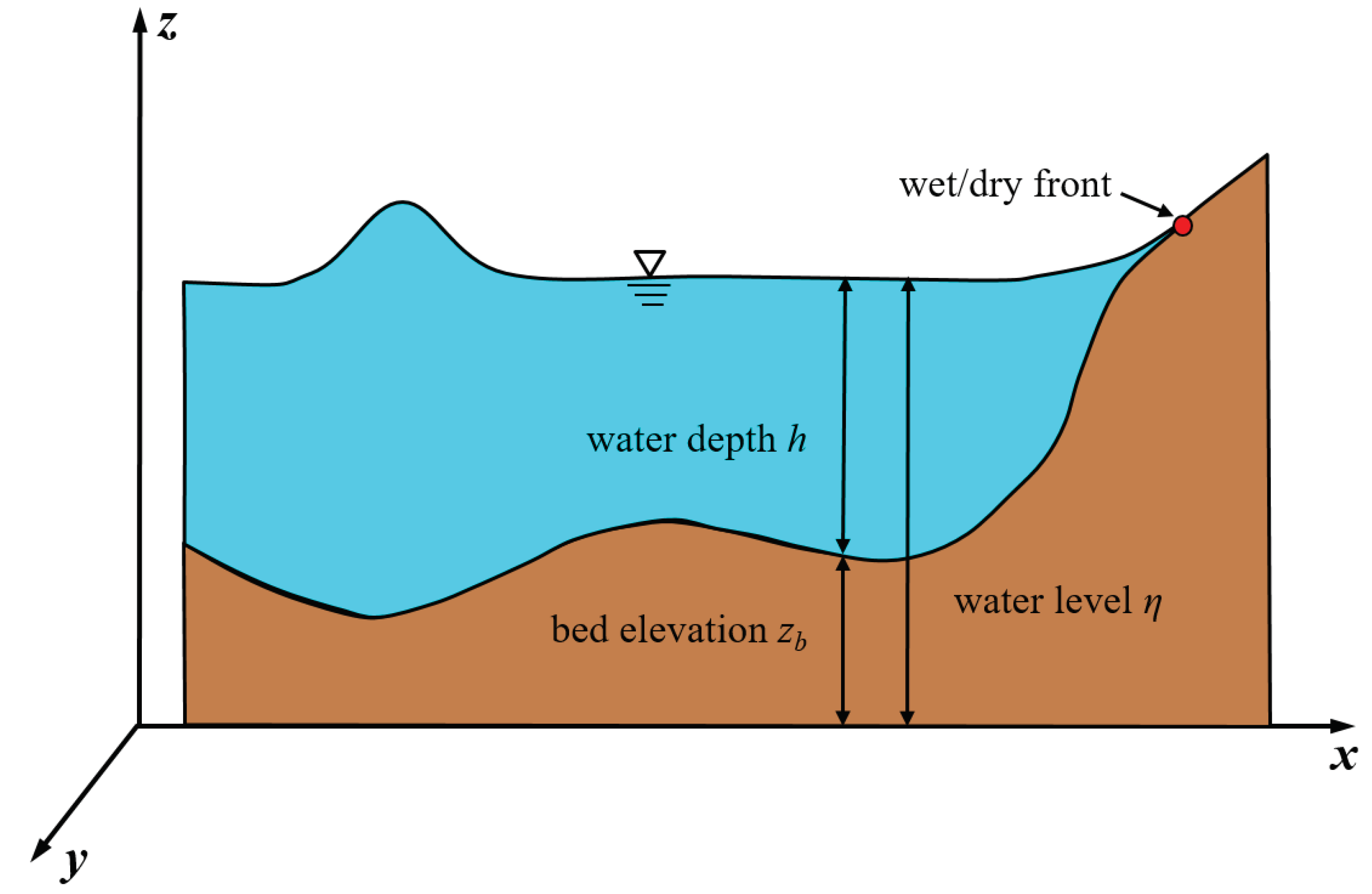
where u, v, and w are the mean velocities in the x, y, and z directions shown in Figure 1, respectively; t is time; $\rho$ is the fluid density; g represents the gravitational acceleration. Assume that the Reynolds stresses are dominant over the fluid shear stresses and ${\tau }_{ij}$(i, $j=x$, y, z) are the turbulent stresses. P is the mean pressure. The pressure can be divided as the hydrostatic part p and non-hydrostatic part $\mathsf{\Gamma }$, which is:

$$P=p+\mathsf{\Gamma }$$

(5)

where p linearly increases with water depth.

According to the assumption made in Stelling and Zijlema [9], the non-hydrostatic $\mathsf{\Gamma }$ and vertical velocity w changes linearly with water depth. The depth-averaged non-hydrostatic pressure $\overline{\mathsf{\Gamma }}$ and vertical velocity $\overline{w}$ is thus shown as follows:

$$\overline{\mathsf{\Gamma }}=\frac{1}{2}({\mathsf{\Gamma }}_s+{\mathsf{\Gamma }}_b)$$

(6)

$$\overline{w}=\frac{1}{2}(w_s+w_b)$$

(7)

where subscripts s and b mean surface and bottom, respectively. In general, non-hydrostatic pressure at the surface ${\mathsf{\Gamma }}_s$ is set to 0.

Assuming that the bed elevation is fixed ($\partial z_b/\partial t=0$), then the kinematic surface and bottom boundary conditions are:

$$w_s=\frac{d\eta }{dt}=\frac{\partial \eta }{\partial t}+u_s\frac{\partial \eta }{\partial x}+v_s\frac{\partial \eta }{\partial y}$$

(8)

$$w_b=\frac{d{z}_b}{dt}=u_b\frac{\partial z_b}{\partial x}+v_b\frac{\partial z_b}{\partial y}$$

(9)

where $\eta$ is the water surface fluctuation; $z_b$ is bottom elevation, which is assumed constant for fixed bottom conditions. The relationship between $\eta$, h, and $z_b$ is shown in Figure 1.

By inserting Equation (5) into Equations (2)–(4), integrating the equations along the vertical direction, and introducing Equations (6) to (9) and the turbulent stress at the bottom boundary ${({\tau }_{xz})}_b=\rho g\overline{u}\sqrt{{\overline{u}}^2+{\overline{v}}^2}{n}^2/h^{1/3}$ ${({\tau }_{yz})}_b=\rho g\overline{v}\sqrt{{\overline{u}}^2+{\overline{v}}^2}{n}^2/h^{1/3}$, the depth-averaged governing equations for the two-dimensional non-hydrostatic model are:

$$\frac{\partial \eta }{\partial t}+\frac{\partial h\overline{u}}{\partial x}+\frac{\partial h\overline{v}}{\partial y}=0$$

(10)

$$\frac{\partial h\overline{u}}{\partial t}+\frac{\partial (h{\overline{u}}^2+\frac{1}{2}g{h}^2)}{\partial x}+\frac{\partial h\overline{v}\overline{u}}{\partial y}=-gh\frac{\partial z_b}{\partial x}-\frac{g\overline{u}\sqrt{{\overline{u}}^2+{\overline{v}}^2}{n}^2}{h^{1/3}}-\frac{h}{2\rho }\frac{\partial {\mathsf{\Gamma }}_b}{\partial x}-\frac{{\mathsf{\Gamma }}_b}{2\rho }\frac{\partial (\eta +z_b)}{\partial x}$$

(11)

$$\frac{\partial h\overline{v}}{\partial t}+\frac{\partial h\overline{v}\overline{u}}{\partial x}+\frac{\partial (h{\overline{v}}^2+\frac{1}{2}g{h}^2)}{\partial y}=-gh\frac{\partial z_b}{\partial y}-\frac{g\overline{v}\sqrt{{\overline{u}}^2+{\overline{v}}^2}{n}^2}{h^{1/3}}-\frac{h}{2\rho }\frac{\partial {\mathsf{\Gamma }}_b}{\partial y}-\frac{{\mathsf{\Gamma }}_b}{2\rho }\frac{\partial (\eta +z_b)}{\partial y}$$

(12)

$$\frac{\partial \overline{w}}{\partial t}=\frac{{\mathsf{\Gamma }}_b}{\rho h}$$

(13)

where overbar “–” denotes the average quantity, and n is the Manning’s coefficient. For convenience, the overbar “–” symbol will be dropped afterward, and u and v represent the averaged velocity in the x and y directions in the following section.

In order to present this numerical method clearly and compactly, Equations (10)–(12) are rewritten in vector forms:

$$\frac{\partial \mathit{q}}{\partial t}+\frac{\partial \mathit{f}}{\partial x}+\frac{\partial \mathit{g}}{\partial y}=\mathit{s}$$

(14)

$$\mathit{q}=\left[\begin{array}{c}\eta \\ hu\\ hv\end{array}\right]\mathit{f}=\left[\begin{array}{c}hu\\ h{u}^2+\frac{1}{2}g{h}^2\\ huv\end{array}\right]\mathit{g}=\left[\begin{array}{c}hv\\ huv\\ h{v}^2+\frac{1}{2}g{h}^2\end{array}\right]$$

$$\mathit{s}={\mathit{s}}_h+{\mathit{s}}_f+{\mathit{s}}_p=\left[\begin{array}{c}0\\ -gh\frac{\partial z_b}{\partial x}\\ -gh\frac{\partial z_b}{\partial y}\end{array}\right]+\left[\begin{array}{c}0\\ -\frac{gu\sqrt{u^2+v^2}{n}^2}{h^{1/3}}\\ -\frac{gv\sqrt{u^2+v^2}{n}^2}{h^{1/3}}\end{array}\right]+\left[\begin{array}{c}0\\ -\frac{h}{2\rho }\frac{\partial {\mathsf{\Gamma }}_b}{\partial x}-\frac{{\mathsf{\Gamma }}_b}{2\rho }\frac{\partial (\eta +z_b)}{\partial x}\\ -\frac{h}{2\rho }\frac{\partial {\mathsf{\Gamma }}_b}{\partial y}-\frac{{\mathsf{\Gamma }}_b}{2\rho }\frac{\partial (\eta +z_b)}{\partial y}\end{array}\right]$$

where $\mathit{q}$ is a vector of the conserved variables; $\mathit{f}$ and $\mathit{g}$ are the flux vectors in the x and y direction, respectively; $\mathit{s}$ is the source term vectors including the bed slope term ${\mathit{s}}_h$, bed friction term ${\mathit{s}}_f$, and non-hydrostatic pressure term ${\mathit{s}}_p$.

2.2. Numerical Methods

The calculation of the two-dimensional non-hydrostatic wave model is divided into two steps. The first step is to solve the governing equations for hydrostatic pressure, and the non-hydrostatic pressure is then calculated.

2.2.1. Calculation of the Hydrostatic Pressure Term

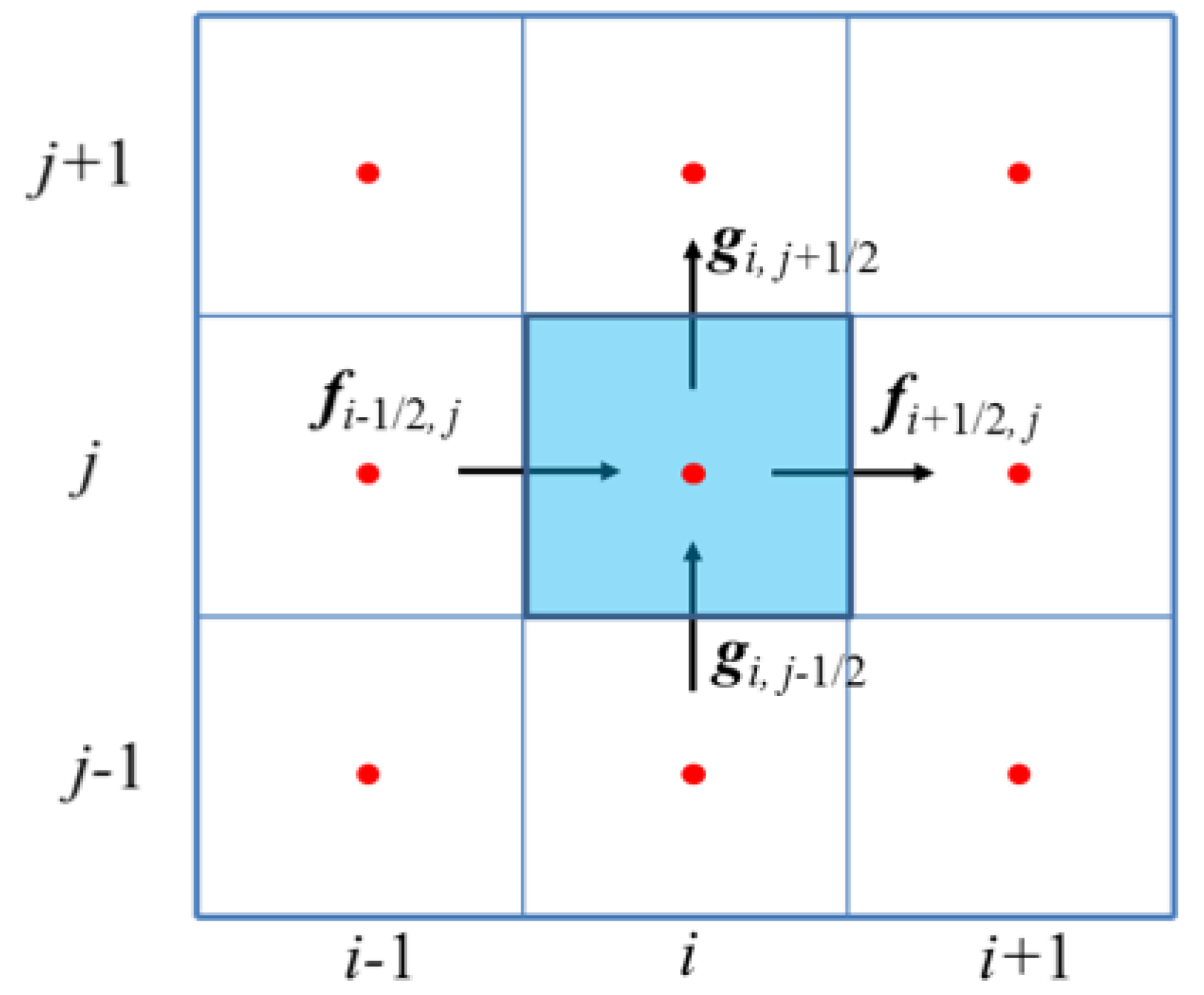
The governing equations for hydrostatic pressure means that the source term $\mathit{s}$ in Equation (14) only include the bed slope term ${\mathit{s}}_h$ and bed friction term ${\mathit{s}}_f$. Therefore, the governing equations are actually the nonlinear shallow water equations (NLSWEs). In this study, the mathematical model is discretized using a finite volume method based on a rectangular mesh with a non-staggered (collocated) grid system, as shown in Figure 2.

Integrating Equation (14) over the (i, j) control volume, applying the Green’s theorem, and using the second order Runge-Kutta method for the time derivative, the discretization of Equation (14) is:

$${\mathit{q}}_{i,j}^{o+1}={\mathit{q}}_{i,j}^o+0.5\Delta t[D({\mathit{q}}_{i,j}^o)+D({\mathit{q}}_{i,j}^{o+1/2})]$$

(15)

$${\mathit{q}}_{i,j}^{o+1/2}={\mathit{q}}_{i,j}^o+\Delta tD({\mathit{q}}_{i,j}^o)$$

(16)

where superscript o is the o-th time step; subscripts i, j are the grid indexes; $\Delta t$ is the time step, and the operator $D({\mathit{q}}_{i,j})$ is defined as:

$$D({\mathit{q}}_{i,j})=-\frac{({\mathit{f}}_{i+1/2,j}-{\mathit{f}}_{i-1/2,j})}{\Delta x}-\frac{({\mathit{g}}_{i,j+1/2}-{\mathit{g}}_{i,j-1/2})}{\Delta y}+({\mathit{s}}_{hi,j}+{\mathit{s}}_{fi,j})$$

(17)

where $\Delta x$ and $\Delta y$ are the cell lengths in x and y directions, ${\mathit{f}}_{i+1/2,j}$ and ${\mathit{f}}_{i-1/2,j}$ are the fluxes at faces $(i+1/2,j)$ and $(i-1/2,j)$. ${\mathit{g}}_{i,j+1/2}$ and ${\mathit{g}}_{i,j-1/2}$ are the fluxes at faces $(i,j+1/2)$ and $(i,j-1/2)$. ${\mathit{s}}_{hi,j}$ and ${\mathit{s}}_{fi,j}$ represent the source terms evaluated at the cell center.

To preserve the well-balanced property, the nonnegative reconstruction procedure proposed by Liang [30] is used in the present model (see the detail in Appendix A). Moreover, the model adopts a MUSCL interpolation with minmod limiter to achieve second order accuracy in space. Further details of MUSCL interpolation are given in Appendix A. To solve Equation (15), the central-upwind scheme is used to calculate convective fluxes at cell interfaces, which is written as:

$${\mathit{f}}_{cu}=\frac{a^{+}{\mathit{f}}^L-a^{-}{\mathit{f}}^R}{a^{+}-a^{-}}+\frac{a^{+}{a}^{-}}{a^{+}-a^{-}}({\mathit{q}}^R-{\mathit{q}}^L)$$

(18)

where superscript L and R represent the reconstructed states at the left and right side of the cell interface, respectively, and $a^{+}$ and $a^{-}$ denote one-sided local wave speeds, which are estimated as:

$$a^{+}=\max (V^R+\sqrt{g{h}^R},V^L+\sqrt{g{h}^L},0)a^{-}=\min (V^R-\sqrt{g{h}^R},V^L-\sqrt{g{h}^L},0)$$

(19)

where V is the velocity at the cell interface. For the treatment of wet/dry front, the bed slope term ${\mathit{s}}_h$ and bed friction term ${\mathit{s}}_f$, one can refer to Appendix A or Wu et al. [29] for more details.

2.2.2. Calculation of the Non-Hydrostatic Pressure Term

The calculation of the non-hydrostatic pressure term ${\mathit{s}}_p$ is to modify the velocity obtained from the hydrostatic pressure calculation. The equations for velocity corrections are:

$$\frac{{(hu)}_{i,j}^{o+1}-{(hu)}_{i,j}^m}{\Delta t}=-\frac{h_{i,j}^m}{2\rho }{(\frac{\partial {\mathsf{\Gamma }}_b}{\partial x})}_{i,j}^{o+1}-\frac{1}{2\rho }{(\frac{\partial (\eta +z_b)}{\partial x})}_{i,j}^m{({\mathsf{\Gamma }}_b)}_{i,j}^{o+1}$$

(20)

$$\frac{{(hv)}_{i,j}^{o+1}-{(hv)}_{i,j}^m}{\Delta t}=-\frac{h_{i,j}^m}{2\rho }{(\frac{\partial {\mathsf{\Gamma }}_b}{\partial y})}_{i,j}^{o+1}-\frac{1}{2\rho }{(\frac{\partial (\eta +z_b)}{\partial y})}_{i,j}^m{({\mathsf{\Gamma }}_b)}_{i,j}^{o+1}$$

(21)

$$\frac{{(w_s)}_{i,j}^{o+1}+{(w_b)}_{i,j}^{o+1}-{(w_s)}_{i,j}^o-{(w_b)}_{i,j}^o}{2\Delta t}=\frac{{({\mathsf{\Gamma }}_b)}_{i,j}^{o+1}}{\rho h_{i,j}^m}$$

(22)

where superscript m represents the results from the hydrostatic calculation.

From the above equations, it can be known that the key to obtain the velocity under non-hydrostatic conditions is to calculate the non-hydrostatic pressure ${({\mathsf{\Gamma }}_b)}_{i,j}^{o+1}$ at the new time step $o+1$. In Equation (22), ${(w_b)}_{i,j}^{o+1}$ can be calculated according to Equation (9), which is:

$${(w_b)}_{i,j}^{o+1}\approx u_{i,j}^m\frac{{(z_b)}_{i+1,j}-{(z_b)}_{i-1,j}}{2\Delta x}+v_{i,j}^m\frac{{(z_b)}_{i,j+1}-{(z_b)}_{i,j-1}}{2\Delta y}$$

(23)

By re-discretizing Equations (20) and (21) at the cell interfaces, the following equations can be obtained:

$$\frac{{(hu)}_{i+1/2,j}^{o+1}-{(hu)}_{i+1/2,j}^m}{\Delta t}=-\frac{h_{i+1/2,j}^m}{2\rho }\frac{{({\mathsf{\Gamma }}_b)}_{i+1,j}^{o+1}-{({\mathsf{\Gamma }}_b)}_{i,j}^{o+1}}{\Delta x}-\frac{1}{2\rho }{(\frac{\partial (\eta +z_b)}{\partial x})}_{i+1/2,j}^m\frac{{({\mathsf{\Gamma }}_b)}_{i,j}^{o+1}+{({\mathsf{\Gamma }}_b)}_{i+1,j}^{o+1}}{2}$$

(24a)

$$\frac{{(hu)}_{i-1/2,j}^{o+1}-{(hu)}_{i-1/2,j}^m}{\Delta t}=-\frac{h_{i-1/2,j}^m}{2\rho }\frac{{({\mathsf{\Gamma }}_b)}_{i,j}^{o+1}-{({\mathsf{\Gamma }}_b)}_{i-1,j}^{o+1}}{\Delta x}-\frac{1}{2\rho }{(\frac{\partial (\eta +z_b)}{\partial x})}_{i-1/2,j}^m\frac{{({\mathsf{\Gamma }}_b)}_{i,j}^{o+1}+{({\mathsf{\Gamma }}_b)}_{i-1,j}^{o+1}}{2}$$

(24b)

$$\frac{{(hv)}_{i,j+1/2}^{o+1}-{(hv)}_{i,j+1/2}^m}{\Delta t}=-\frac{h_{i,j+1/2}^m}{2\rho }\frac{{({\mathsf{\Gamma }}_b)}_{i,j+1}^{o+1}-{({\mathsf{\Gamma }}_b)}_{i,j}^{o+1}}{\Delta y}-\frac{1}{2\rho }{(\frac{\partial (\eta +z_b)}{\partial y})}_{i,j+1/2}^m\frac{{({\mathsf{\Gamma }}_b)}_{i,j}^{o+1}+{({\mathsf{\Gamma }}_b)}_{i,j+1}^{o+1}}{2}$$

(24c)

$$\frac{{(hv)}_{i,j-1/2}^{o+1}-{(hv)}_{i,j-1/2}^m}{\Delta t}=-\frac{h_{i,j-1/2}^m}{2\rho }\frac{{({\mathsf{\Gamma }}_b)}_{i,j}^{o+1}-{({\mathsf{\Gamma }}_b)}_{i,j-1}^{o+1}}{\Delta y}-\frac{1}{2\rho }{(\frac{\partial (\eta +z_b)}{\partial y})}_{i,j-1/2}^m\frac{{({\mathsf{\Gamma }}_b)}_{i,j}^{o+1}+{({\mathsf{\Gamma }}_b)}_{i,j-1}^{o+1}}{2}$$

(24d)

Assumming that

$${(hu)}_{i+1/2,j}^{o+1}\approx h_{i+1/2,j}^m{u}_{i+1/2,j}^{o+1}$$

(25a)

$${(hu)}_{i-1/2,j}^{o+1}\approx h_{i-1/2,j}^m{u}_{i-1/2,j}^{o+1}$$

(25b)

After some mathematical manipulations, the velocity in x direction at interface ($i+1/2,j$) and ($i-1/2,j$) can be written as

$$u_{i+1/2,j}^{o+1}=u_{i+1/2,j}^m-\frac{\Delta t}{2\rho }\frac{{({\mathsf{\Gamma }}_b)}_{i+1,j}^{o+1}-{({\mathsf{\Gamma }}_b)}_{i,j}^{o+1}}{\Delta x}-\frac{\Delta t}{2\rho h_{i+1/2,j}^m}{(\frac{\partial (\eta +z_b)}{\partial x})}_{i+1/2,j}^m\frac{{({\mathsf{\Gamma }}_b)}_{i,j}^{o+1}+{({\mathsf{\Gamma }}_b)}_{i+1,j}^{o+1}}{2}$$

(26a)

$$u_{i-1/2,j}^{o+1}=u_{i-1/2,j}^m-\frac{\Delta t}{2\rho }\frac{{({\mathsf{\Gamma }}_b)}_{i,j}^{o+1}-{({\mathsf{\Gamma }}_b)}_{i-1,j}^{o+1}}{\Delta x}-\frac{\Delta t}{2\rho h_{i-1/2,j}^m}{(\frac{\partial (\eta +z_b)}{\partial x})}_{i-1/2,j}^m\frac{{({\mathsf{\Gamma }}_b)}_{i,j}^{o+1}+{({\mathsf{\Gamma }}_b)}_{i-1,j}^{o+1}}{2}$$

(26b)

The similar procedure is applied to obtain $v_{i,j+1/2}^{o+1}$ and $v_{i,j-1/2}^{o+1}$.

Bottom non-hydrostatic pressure at the new time step can be evaluated through Equation (1), and the corresponding implicit discretized equations are:

$$\frac{u_{i+1/2,j}^{o+1}-u_{i-1/2,j}^{o+1}}{\Delta x}+\frac{v_{i,j+1/2}^{o+1}-v_{i,j-1/2}^{o+1}}{\Delta y}+\frac{{(w_s)}_{i,j}^{o+1}-{(w_b)}_{i,j}^{o+1}}{h_{i,j}^m}=0$$

(27)

Inserting Equations (23) and (26) into Equation (27), the linear equations (Poisson equations) for ${\mathsf{\Gamma }}_b$ are given below:

$$A_{i,j}{({\mathsf{\Gamma }}_b)}_{i-1,j}^{o+1}+B_{i,j}{({\mathsf{\Gamma }}_b)}_{i,j}^{o+1}+C_{i,j}{({\mathsf{\Gamma }}_b)}_{i+1,j}^{o+1}+D_{i,j}{({\mathsf{\Gamma }}_b)}_{i,j-1}^{o+1}+E_{i,j}{({\mathsf{\Gamma }}_b)}_{i,j+1}^{o+1}=S_{i,j}$$

(28)

where the coefficients are:

$$A_{i,j}=-\frac{\Delta t}{2\rho {\Delta }^{2}x}-\frac{\Delta t}{2\rho {\Delta }^{2}x}\frac{{\eta }_{i,j}^m+{(z_b)}_{i,j}-{\eta }_{i-1,j}^m-{(z_b)}_{i-1,j}}{h_{i,j}^m+h_{i-1,j}^m}$$

(29a)

$$\begin{array}{cc}\hfill B_{i,j}=& \frac{2\Delta t}{\rho {(h_{i,j}^m)}^2}+\frac{\Delta t}{\rho {\Delta }^{2}x}+\frac{\Delta t}{\rho {\Delta }^{2}y}\hfill \\ \hfill +& \frac{\Delta t}{2\rho {\Delta }^{2}x}[\frac{{\eta }_{i+1,j}^m+{(z_b)}_{i+1,j}-{\eta }_{i,j}^m-{(z_b)}_{i,j}}{h_{i,j}^m+h_{i+1,j}^m}-\frac{{\eta }_{i,j}^m+{(z_b)}_{i,j}-{\eta }_{i-1,j}^m-{(z_b)}_{i-1,j}}{h_{i,j}^m+h_{i-1,j}^m}]\hfill \\ \hfill +& \frac{\Delta t}{2\rho {\Delta }^{2}y}[\frac{{\eta }_{i,j+1}^m+{(z_b)}_{i,j+1}-{\eta }_{i,j}^m-{(z_b)}_{i,j}}{h_{i,j}^m+h_{i,j+1}^m}-\frac{{\eta }_{i,j}^m+{(z_b)}_{i,j}-{\eta }_{i,j-1}^m-{(z_b)}_{i,j-1}}{h_{i,j}^m+h_{i,j-1}^m}]\hfill \end{array}$$

(29b)

$$C_{i,j}=-\frac{\Delta t}{2\rho {\Delta }^{2}x}+\frac{\Delta t}{2\rho {\Delta }^{2}x}\frac{{\eta }_{i+1,j}^m+{(z_b)}_{i+1,j}-{\eta }_{i,j}^m-{(z_b)}_{i,j}}{h_{i,j}^m+h_{i+1,j}^m}$$

(29c)

$$D_{i,j}=-\frac{\Delta t}{2\rho {\Delta }^{2}y}+\frac{\Delta t}{2\rho {\Delta }^{2}y}\frac{{\eta }_{i,j}^m+{(z_b)}_{i,j}-{\eta }_{i,j-1}^m-{(z_b)}_{i,j-1}}{h_{i,j}^m+h_{i,j-1}^m}$$

(29d)

$$E_{i,j}=-\frac{\Delta t}{2\rho {\Delta }^{2}y}+\frac{\Delta t}{2\rho {\Delta }^{2}y}\frac{{\eta }_{i,j+1}^m+{(z_b)}_{i,j+1}-{\eta }_{i,j}^m-{(z_b)}_{i,j}}{h_{i,j}^m+h_{i,j+1}^m}$$

(29e)

$$S_{i,j}=-\frac{u_{i+1/2,j}^m-u_{i-1/2,j}^m}{\Delta x}-\frac{v_{i,j+1/2}^m-v_{i,j-1/2}^m}{\Delta y}+\frac{2{(w_b)}_{i,j}^{o+1}-{(w_s)}_{i,j}^o-{(w_b)}_{i,j}^o}{h_{i,j}^m}$$

(29f)

In this study, the biconjugate gradient stabilized method is adopted to solve ${({\mathsf{\Gamma }}_b)}_{i,j}^{o+1}$ in Equation (28), and ${({\mathsf{\Gamma }}_b)}_{i,j}^{o+1}$ is then inserted into Equations (20)–(22) to obtain the velocity $u^{o+1}$, $v^{o+1}$ and $w_s^{o+1}$.

2.2.3. Stability Criterion and Boundary Conditions

Since the current numerical scheme is explicit, its stability is determined by the Courant-Friedrichs-Lewy (CFL) criterion. In order to ensure the stability of the model at each time step, the Courant number $N_{CFL}$ has to be kept less than 0.25 [29]. In this study, the Courant number $N_{CFL}$ is set to be less than 0.20 for all simulations, which is

$$N_{CFL}=\frac{a\Delta t}{\min (\Delta x,\Delta y)}\le 0.2$$

(30)

where a is given by:

$$a=\underset{i,j}{\max }\{a^{+},-a^{-}\}$$

(31)

The ghost-cell is used for the boundary conditions. For the open boundary conditions, flow variables in the ghost cells are usually determined by solving a boundary Riemann problem, which is dependent on the local flow regime. For wall boundary conditions, the velocity normal to the boundary and the water surface gradient are both set to zero at the boundary. For wave inlet boundaries, the variables on the ghost cells are set according to the corresponding analytical formula. For no reflecting boundaries, the sponge layer technique introduced by Larsen and Dancy [31] is employed to fully absorb the incident wave. The following damping coefficient function is used:

$$C_s={\alpha }_s^{r_s^{i-1}},i=1,2,3,\cdots ,n$$

(32)

where ${\alpha }_s$ and $r_s$ are two parameters. n is the number of grid. As suggested by Chen et al. [32], ${\alpha }_s=2$, $r_s=0.88-0.92$ and $n=50-100$ are used in this study.

2.2.4. Manipulation of Wave Breaking Conditions

To deal with the wave breaking conditions, the model adopts the hydrostatic front approximation (HFA) method proposed by Smit et al. [33]. When the temporal variation rate of water levels $\partial \eta /\partial t$ at cells is larger than ${\alpha }_1\sqrt{gh}$ (${\alpha }_1$ is an empirical coefficient and set to 0.6 as Smit et al. [33] suggested in this study), the cell is labeled as wave breaking and the hydrostatic computation is implemented. Therefore, for the wave breaking cells, the non-hydrostatic pressure $\mathsf{\Gamma }$ and vertical velocity w are set to zero.

3. Model Verification

The numerical method presented in the above section is tested with several analytical solutions and laboratory experiments in this section. For all tests, the gravitational acceleration $g=9.8\mathrm{m}/{\mathrm{s}}^2$ and water density $\rho =1000\mathrm{kg}/{\mathrm{m}}^3$.

3.1. Case 1: Propagation of One-Dimensional Solitary Wave in Constant Depth

The first test case is the solitary wave propagation in constant water depth. Solitary wave propagation is extensively used to validate the dispersion characteristics of Boussinesq and non-hydrostatic numerical models. The computational domain is $1000\mathrm{m}$ long and $10\mathrm{m}$ deep with a smooth and flat bottom. The solitary wave is initially at $x_0=200\mathrm{m}$ with wave height $H=2.0\mathrm{m}$. According to the potential flow theorem, the corresponding water level, horizontal and vertical velocities can be obtained, which are [9]:

$$\eta (x,t)=d+H{\mathrm{sech}}^2\left[\sqrt{\frac{3H}{4d^3}}(x-ct-x_0)\right]$$

(33)

$$u(x,t)=\frac{c[\eta (x,t)-d]}{h(x,t)}$$

(34)

$$w_s(x,t)=-\eta (x,t)\frac{\partial u(x,t)}{\partial x}$$

(35)

where d is the still water depth, and $c=\sqrt{g(H+d)}$ is the celerity for the solitary wave.

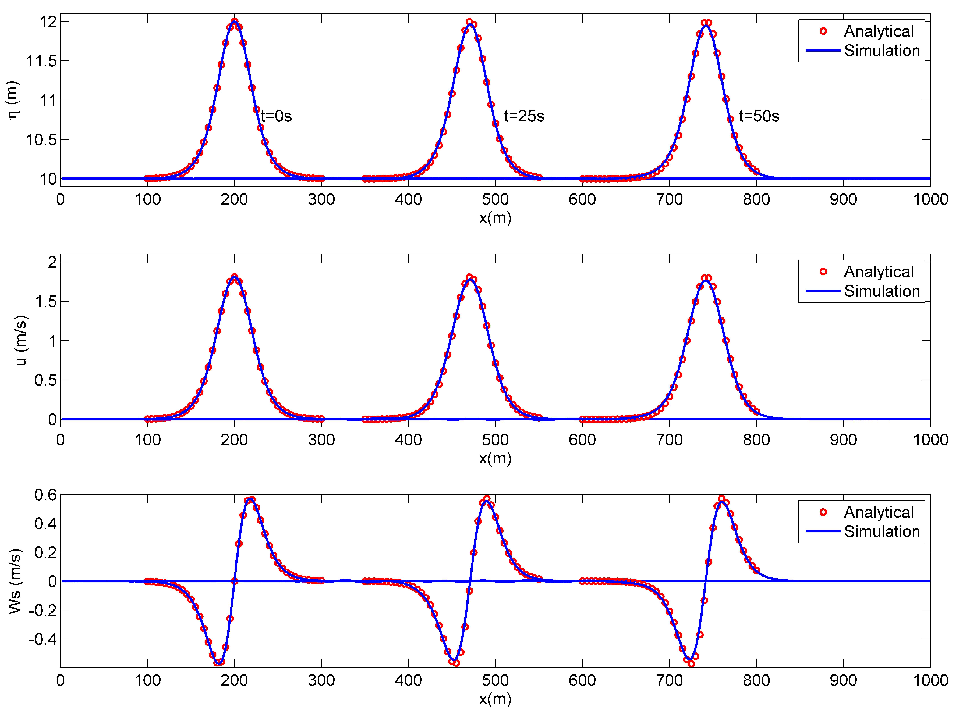
The computational domain is discretized by $2000\times 3$ uniform and rectangular grids with $\Delta x=\Delta y=0.5\mathrm{m}$. The time step $\Delta t$ is adjusted during the simulation based on the Courant number, which is taken as $0.2$. The simulation time is $50\mathrm{s}$. Equations (33)–(35) give the initial water level and velocities at $t=0$. The left and right sides of the computation domain are set as no wave reflection boundaries. Figure 3 shows the comparisons of simulated results (surface elevations and velocities at the surface) and analytic solutions at $t=0$, 25 and $50\mathrm{s}$. The simulations agree well with the analytic results, which means that the developed model can successfully capture the wave feature, and the numerical diffusion almost has no significant impact on the simulations.

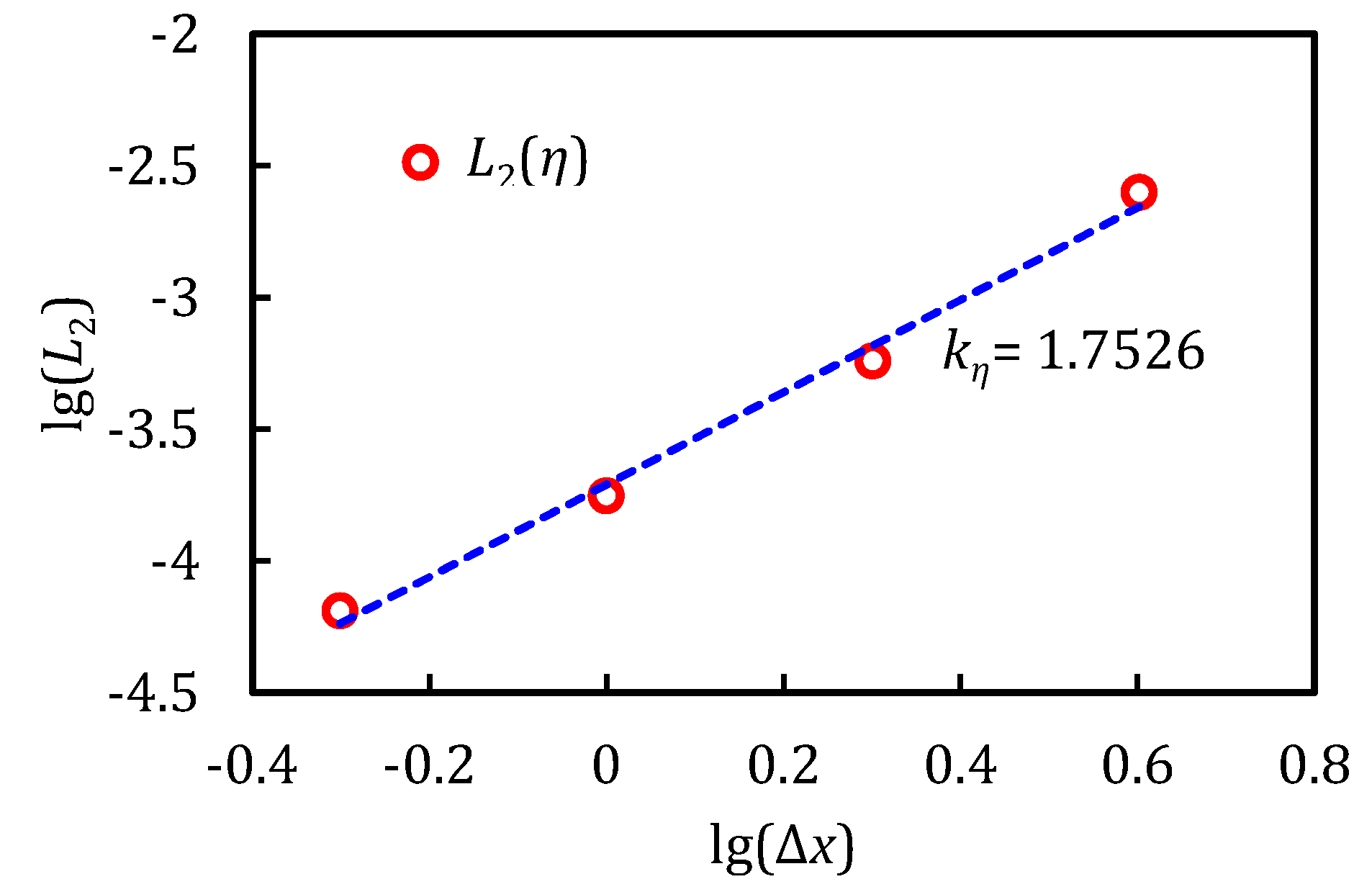
In order to evaluate the order of the accuracy of the model, four different grids with the mesh size of $\Delta x=0.5\mathrm{m}$, $1.0\mathrm{m}$, $2.0\mathrm{m}$ and $4.0\mathrm{m}$ are considered in this study. Figure 4 gives $L_2$ error norms in $\eta$ at $t=50\mathrm{s}$ as a function of grid size $\Delta x$, which is defined as:

$$L_2(\eta )=\frac{1}{N}\sqrt{{\displaystyle \sum _{i=1}^N}{({\eta }_a-{\eta }_i)}^2}$$

(36)

where N is the total number of computational cells, ${\eta }_a$ is the analytical solution. It can be found that the numerical errors are decreased by increasing the number of grids and the accuracy of the present model is close to second-order.

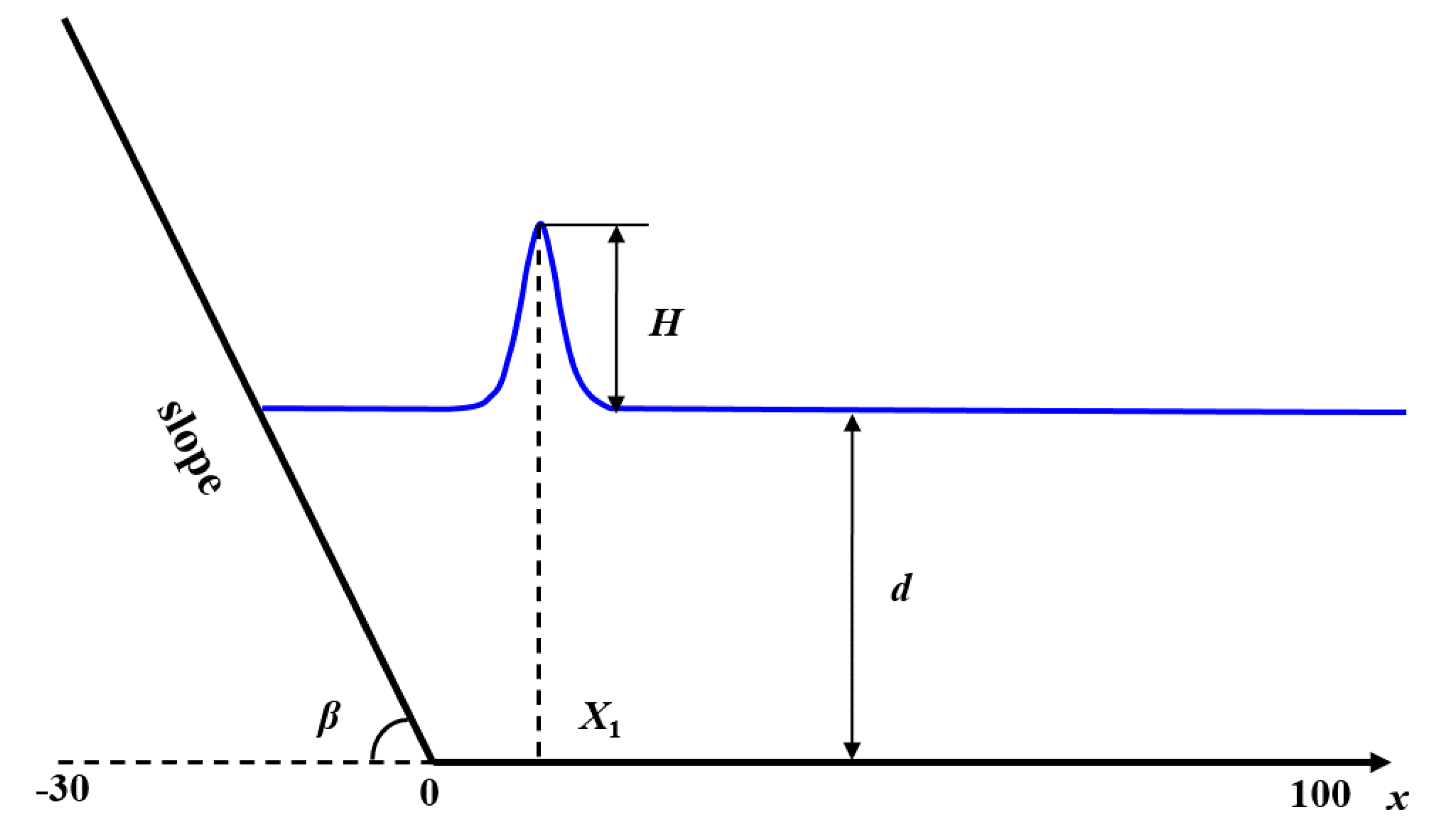
3.2. Case 2: Runup of One-Dimensional Solitary Wave

The experiment for runup of one-dimensional solitary wave conducted by Synolakis [34] is used widely to test the capability of numerical models on dealing with wave breaking and wetting-drying. Figure 5 provides the setup and bottom geometry of the experiment, where H is the wave height of the solitary wave, d is the still water depth, $X_1$ is the location of wave crest and $\beta$ ($={2.884}^{°}$) is the beach slope. The computational domain $x\in [-30,100]$ with the corresponding bathymetry:

$$z_b(x)=\left\{\begin{array}{ll}-x\tan \beta & x\le \cot \beta \\ -1& x>\cot \beta \end{array}\right]$$

(37)

The still water depth d is $1\mathrm{m}$. At $t=0$, the initial surface elevation is as follows:

$$\eta (x)=1+\frac{H}{d}{\mathrm{sech}}^2[\gamma (x-X_1)]$$

(38)

where $\gamma =\sqrt{3H/4d}$ and $X_1=\sqrt{4d/3H}\mathrm{arcosh}(\sqrt{1/0.05})$. The initial horizontal velocity u is:

$$u(x)=-\sqrt{g/d}·\eta (x)$$

(39)

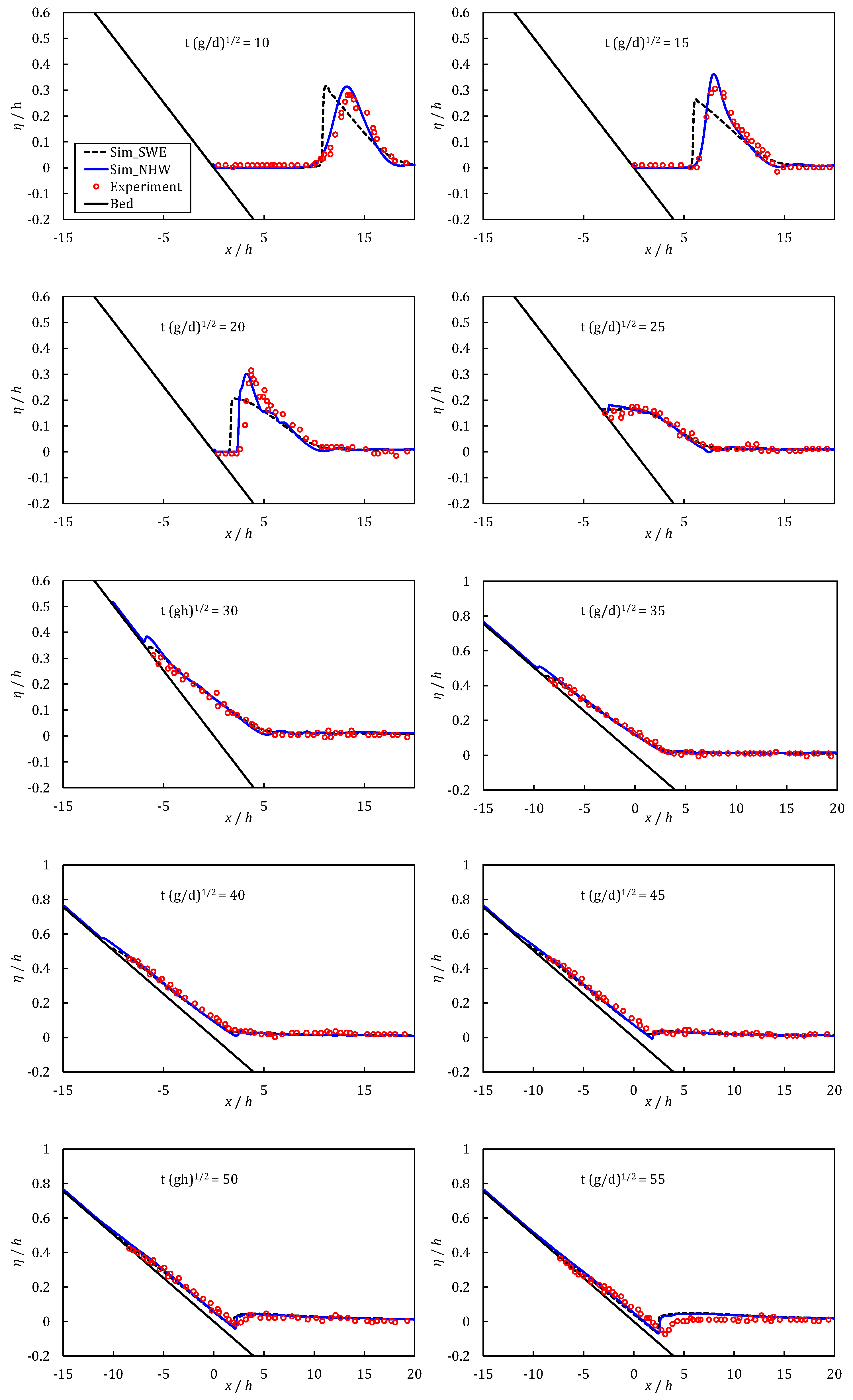
The right-side boundary condition is free outflow, and the Manning’s coefficient n for the whole computational domain is designated as $0.01\mathrm{s}/{\mathrm{m}}^{1/3}$. The grid size is $0.1\times 0.1\mathrm{m}$, and the time step is adaptive. In this study, the numerical simulations using the non-hydrostatic model and shallow water model are compared with the experimental results at $H/d=0.3$.

Figure 6 presents the comparisons of the surface elevation variations at different dimensionless times. At the initial stage, when the incident wave propagates to the shoal, the solitary wave gradually becomes asymmetric, i.e., the wave front steepens, and the wave leeward turns into milder, and the wave height increases as the water depth decreases. It can be seen from Figure 6 that the wave front calculated by the shallow water equation (SWE) is steeper than the experimental results, which is markedly different from the results obtained from the non-hydrostatic wave model (NHW). On the other hand, the NHW method can simulate dispersion characteristics of wave rather well, and the simulation result is in good agreement with the experimental measurements. The main reason for obvious differences in the shallow water model is that it does not contain high-order diffusion terms, leading to its inability to accurately simulate the dispersion effect for the wave motions.

When $t{(g/d)}^{1/2}=25$, because of the shoaling effect, the solitary wave breaks and keeps moving up to the beach. At $t{(g/d)}^{1/2}=40$, the wave climbs to the highest point and then begins to run down. During rundown periods, the flow on the slope becomes supercritical. Since the flow is subcritical over constant depth regions, a hydraulic jump will occur at the toe of the slope. From Figure 6, it can be seen that after wave breaking, the numerical results from the SWE and NHW models are similar. This is because the hydrostatic front approximation (HFA) method is used on wave breaking issues. The essence of the method is that when the wave breaks, the non-hydrostatic model is transformed into the hydrostatic shallow water model, and the non-hydrostatic pressure $\mathsf{\Gamma }$ and vertical velocity w are set to zero. In general, the non-hydrostatic model presented in this study can successfully simulate the breaking solitary wave runup and rundown along a beach.

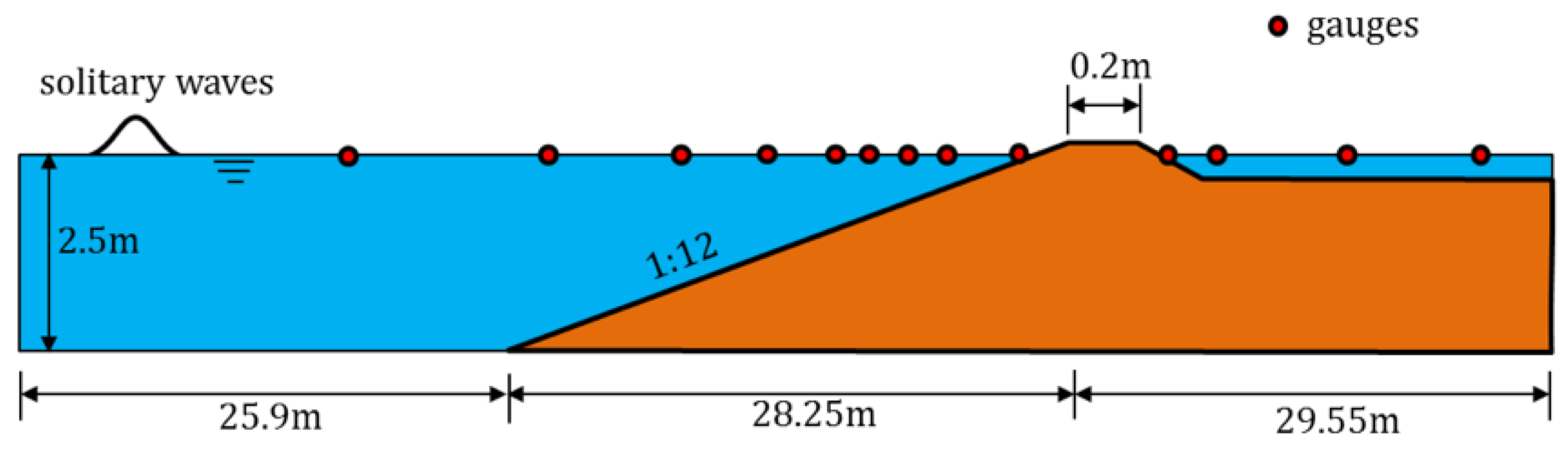
3.3. Case 3: Propagation of Solitary Wave over Fringing Reef

Fringing reef is a kind of coral reef widely existing in tropical and subtropical areas. It connects directly to the coastline and stretches out hundreds to several kilometers. An ideal reef consists of fore reef and reef flat. When the wave passes through the reef, under the action of the slope in front of the reef and the horizontal reef flat, the wave breaks and decays. Therefore, fringing reef plays a protective role in the coastline.

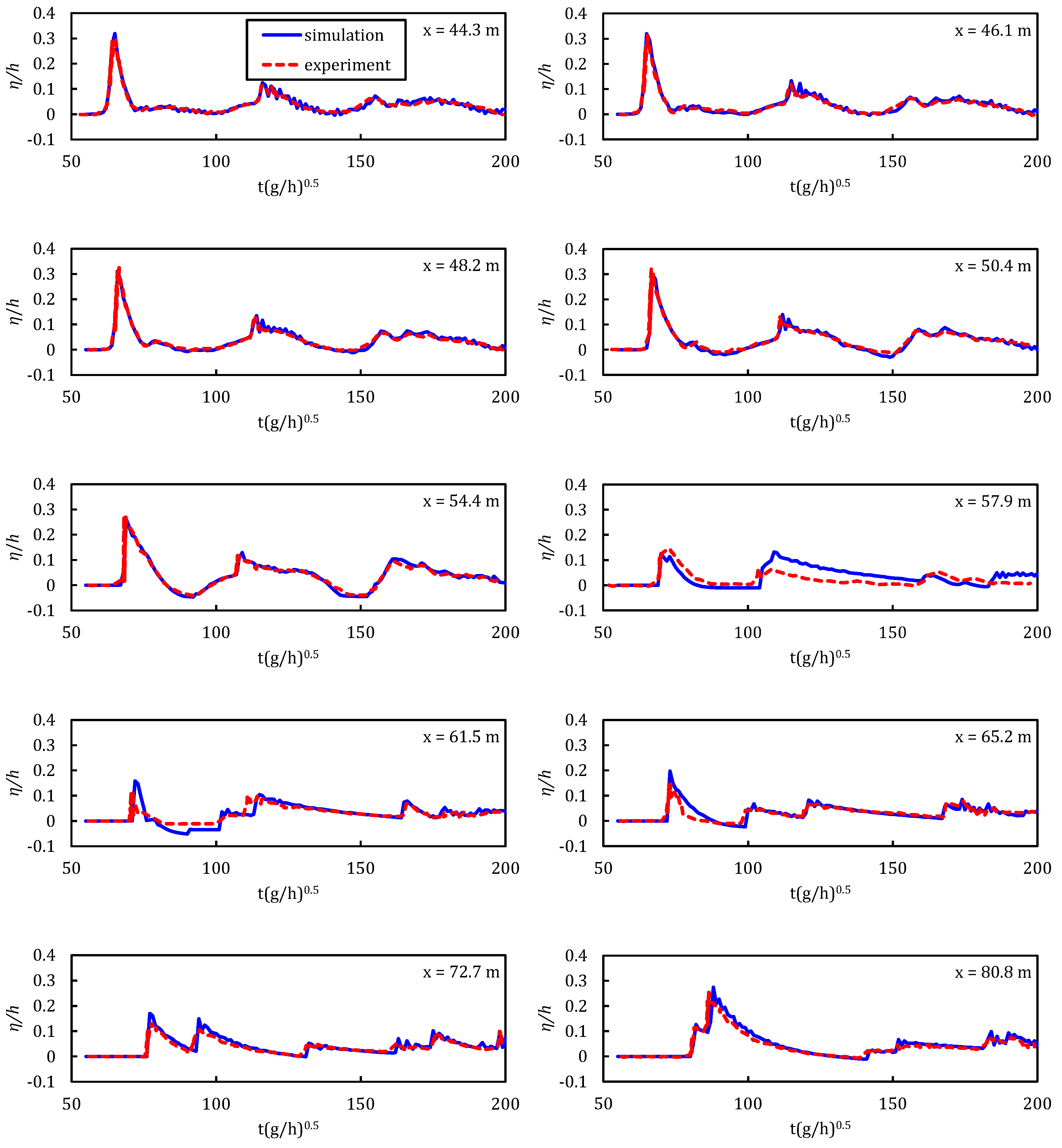
In this study, the propagation and deformation of the solitary wave over the reef is used to examine the ability of the model to deal with wave breaking and wetting and drying. Roeber and Cheung [35] carried out a laboratory experiment to study the propagation and deformation of the solitary wave over the reef. The experimental setup and corresponding geometry is shown in Figure 7. The water is $2.5\mathrm{m}$ deep and the reef flat is submerged by a depth of $0.14\mathrm{m}$. The reef slope is 1:12 with a crest $0.065\mathrm{m}$ above the water level. The wave height of the input solitary wave is $0.75\mathrm{m}$. When the solitary wave propagates into the shallow water, a plunging breaker is developed over the reef. Several water level gauges (red dots on Figure 7) are employed to provide temporal and spatial water level variations.

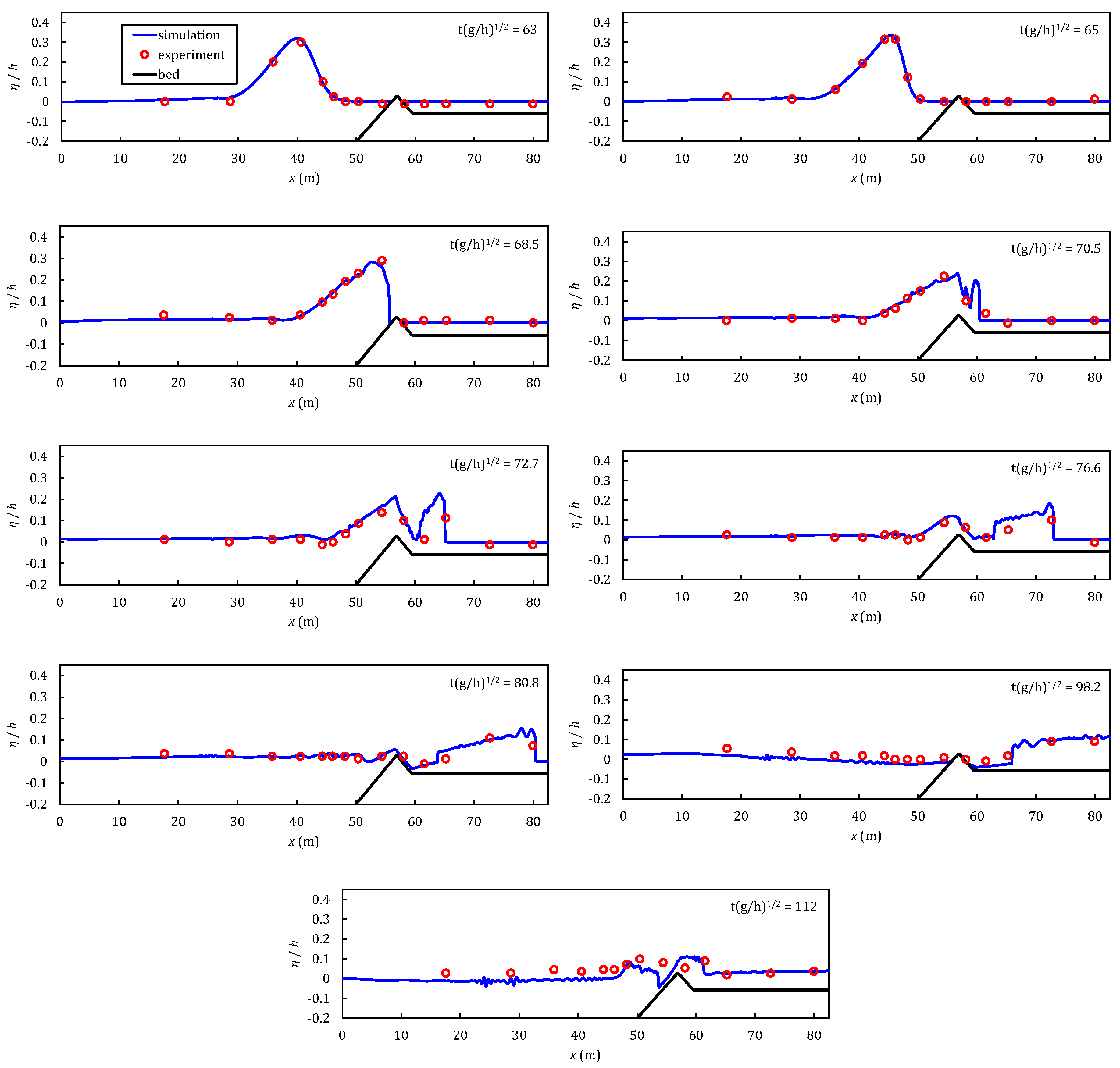
The numerical model uses a grid size $\Delta x=0.05\mathrm{m}$ and a Manning coefficient of $n=0.016\mathrm{s}/{\mathrm{m}}^{1/3}$ to represent the finished concrete surface of the reef model. The time step $\Delta t$ is adaptive to ensure the model stability. As previous examples, the HFA method is used on wave breaking issues. Figure 8 provides the comparison between numerical results and measurements. At $t{(g/d)}^{1/2}=63$ when the solitary wave reaches the reef slope, its wave height increases, and its wave form gradually become asymmetric, i.e., the wave front becomes steeper. At $t{(g/d)}^{1/2}=67$, the wave breaks. When $t{(g/d)}^{1/2}=70.5$, the breaking wave enters the reef flat and leads to a hydraulic jump. At $t{(g/d)}^{1/2}=83$, the wave reaches the right boundary and reflects back to the left side. The reflection wave then jumps over the reef crest and propagates to the upstream. From the comparisons at different times, the computational results are in acceptable agreement with the measurements, which proves that the developed model is able to accurately simulate the processes of solitary wave propagation, breaking and reflection. Figure 9 shows good agreements between the simulated and measured time series of free surface elevation at several wave gauges along the flume centerline, which further confirm the capabilities of the present model to simulate wave motion accurately. It should be noted that the wave amplitudes at 61.5 and 65.2 m are overpredicted by our model, which are also found in the simulation results in Kazolea et al. [36]. A possible explanation is that the flow in this area is very complex and the depth-averaged wave models may not be suitable for this situation.

3.4. Case 4: Runup of Solitary Wave on a Circular Island

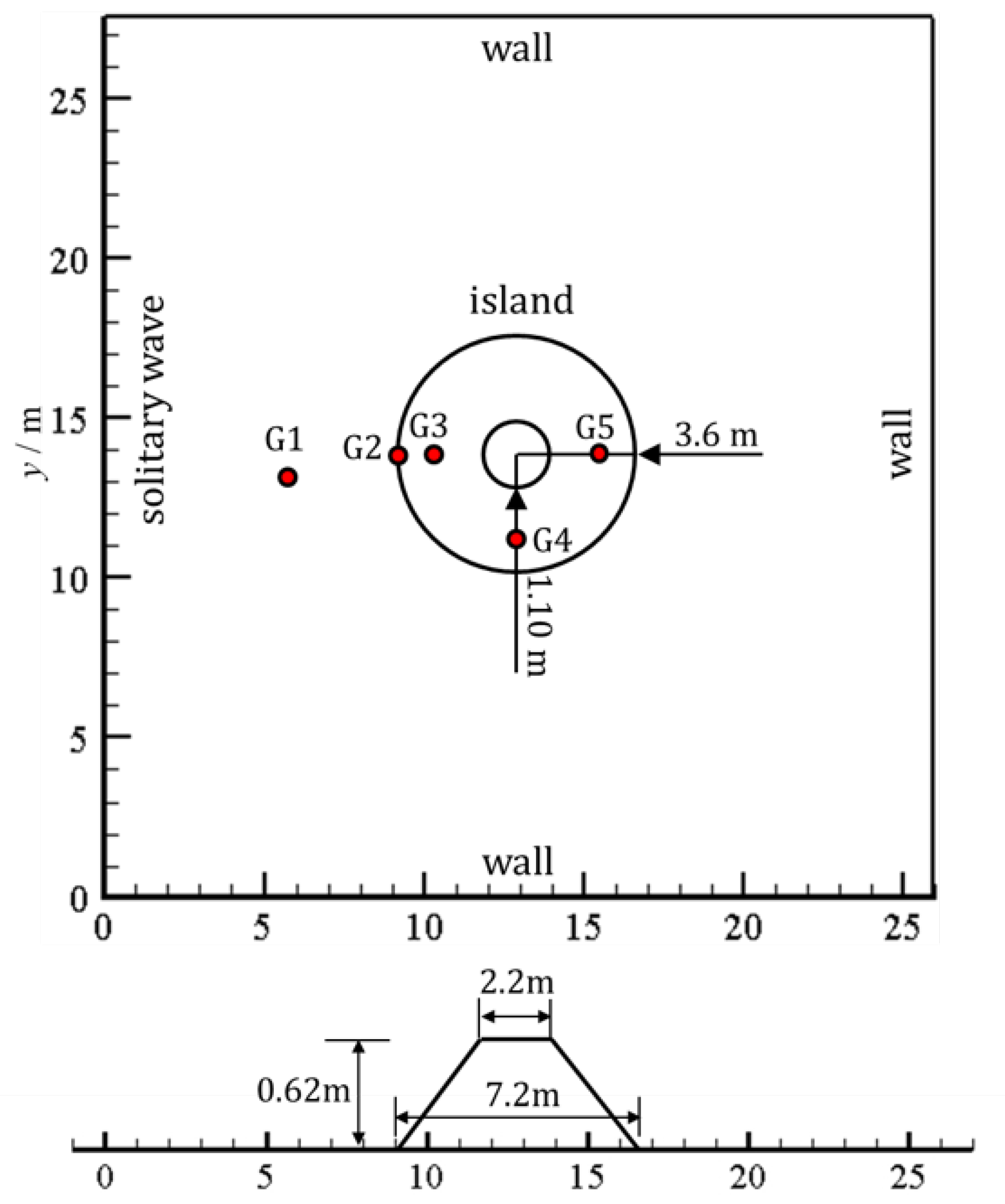
To test the model’s capability of simulating solitary wave runup over a 3D uneven bottom, laboratory experiments conducted by Briggs et al. [37] are used. The model setup and bottom geometry are shown in Figure 10. The physical model of a conical island was constructed in the center of a $30\mathrm{m}$ wide by $25\mathrm{m}$ long flat-bottom wave basin. The island had the shape of a truncated, circular cone with diameters of $7.2\mathrm{m}$ at the toe and $2.2\mathrm{m}$ at the crest, and the height of the cone was $0.625\mathrm{m}$. Data of water surface elevations and wave runup were recorded.

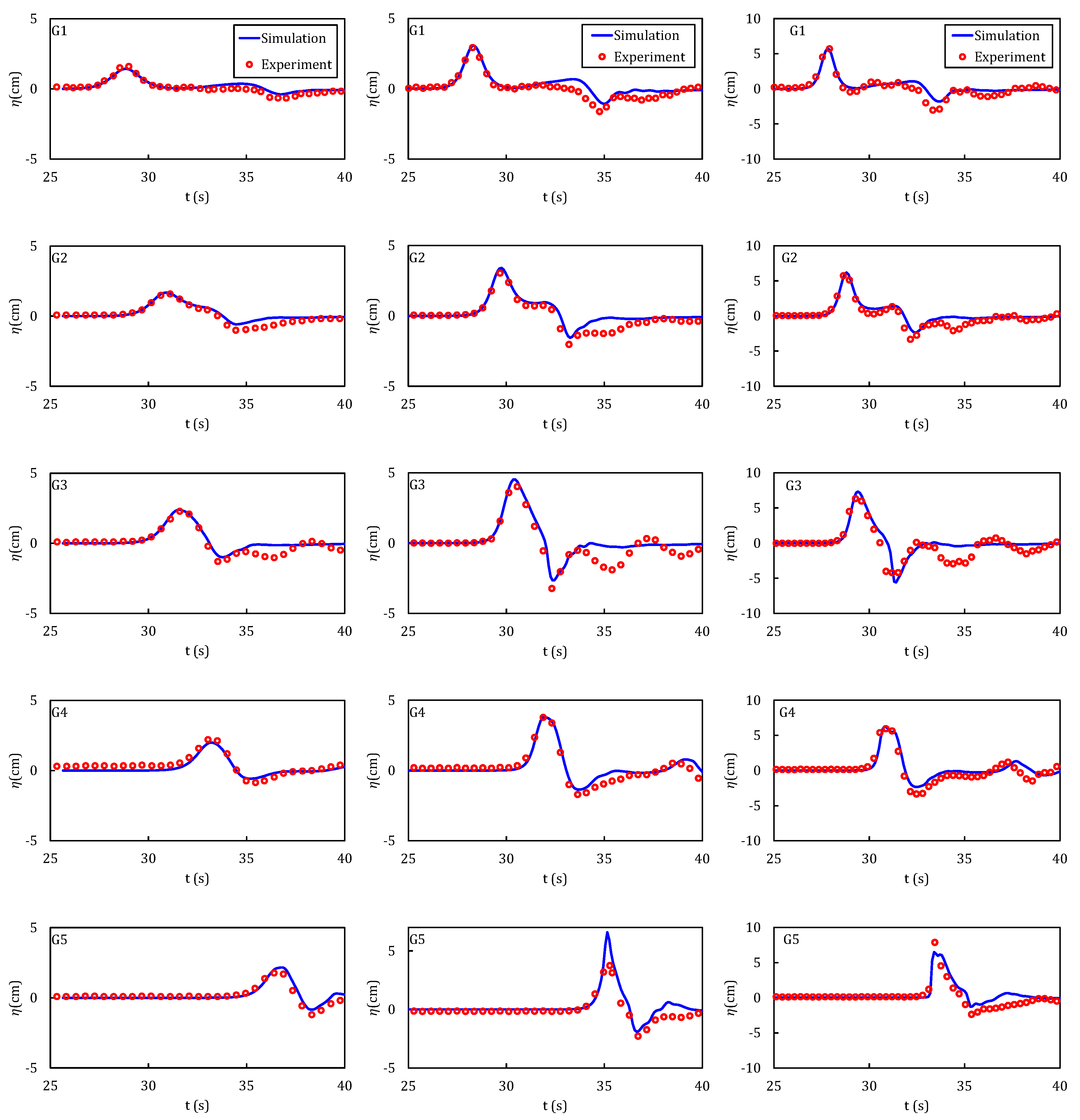
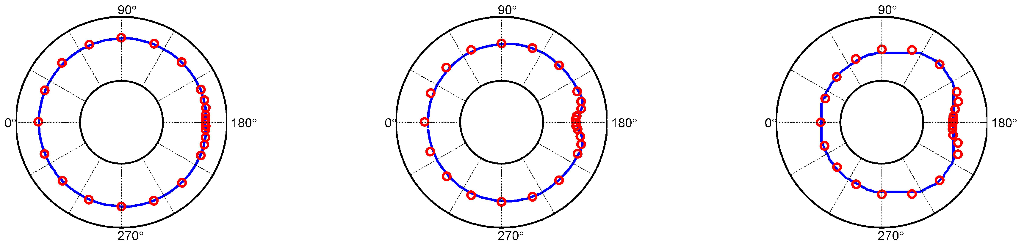
The model is tested under three experimental conditions, which are $H/d=0.045$, $0.096$, and $0.181$, respectively, where the water depth d ($=0.32\mathrm{m}$) is constant. The grid size for the computational domain is $\Delta x=\Delta y=0.05\mathrm{m}$ with the total grid number of 340,000. Since the model is constructed with smooth concrete, the Manning n value is set to zero. The time step is adaptive, and the total simulation time is $40\mathrm{s}$. Figure 11 gives the comparisons of the water level fluctuations between the simulation and measurements. It can be found that overall the simulated water surface fluctuations agree well with the measured data. Figure 12 provides the maximum wave runup along the truncated cone, and shows the simulated values against the measurements. It is, therefore, reasonable to conclude based on the above results, that the model is also able to reproduce the measured wave propagation and runup over a 3D uneven bottom accurately.

3.5. Case 5: Breaking and Runup of Solitary Wave over a Three-Dimensional Complex Bathymetry

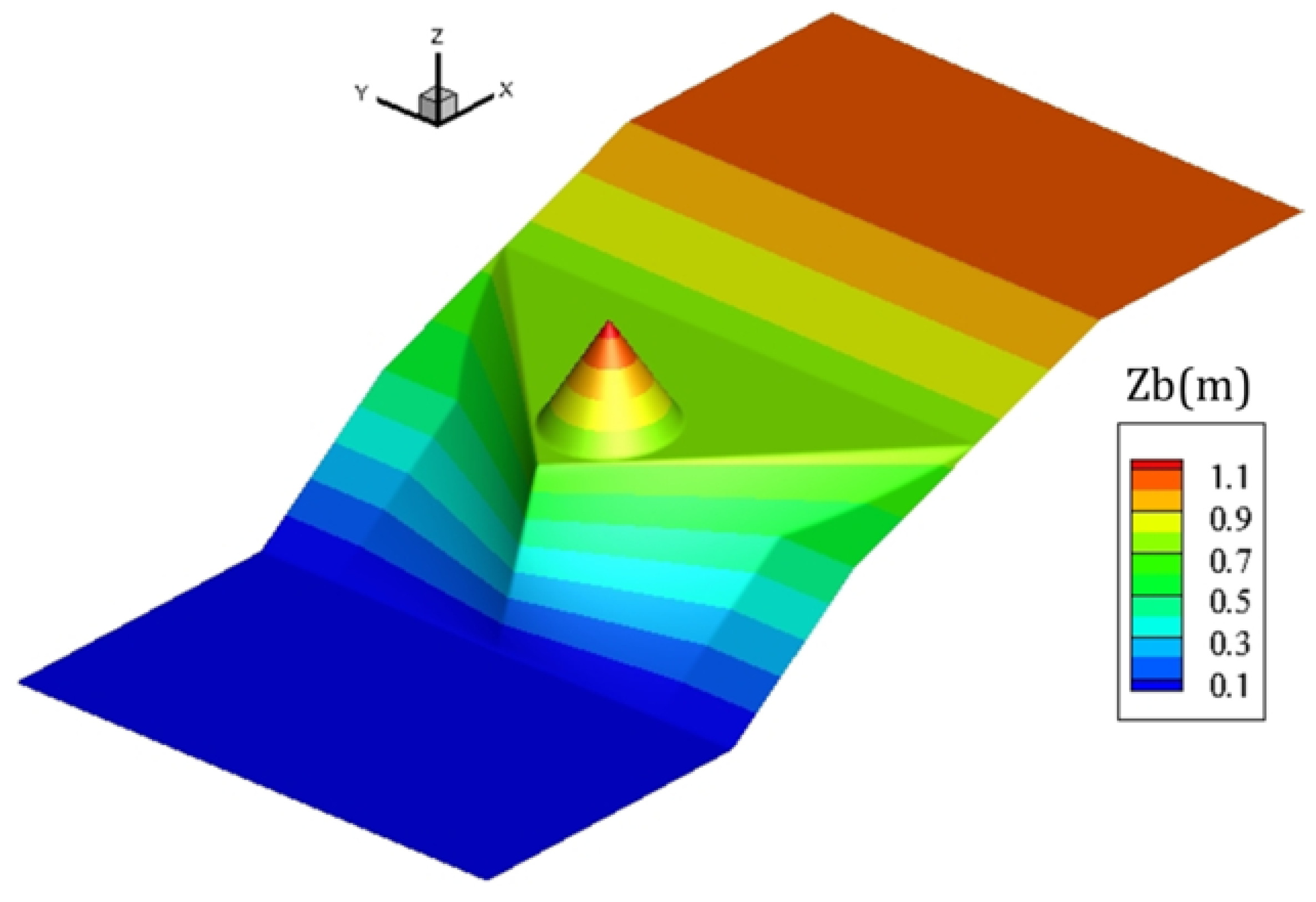
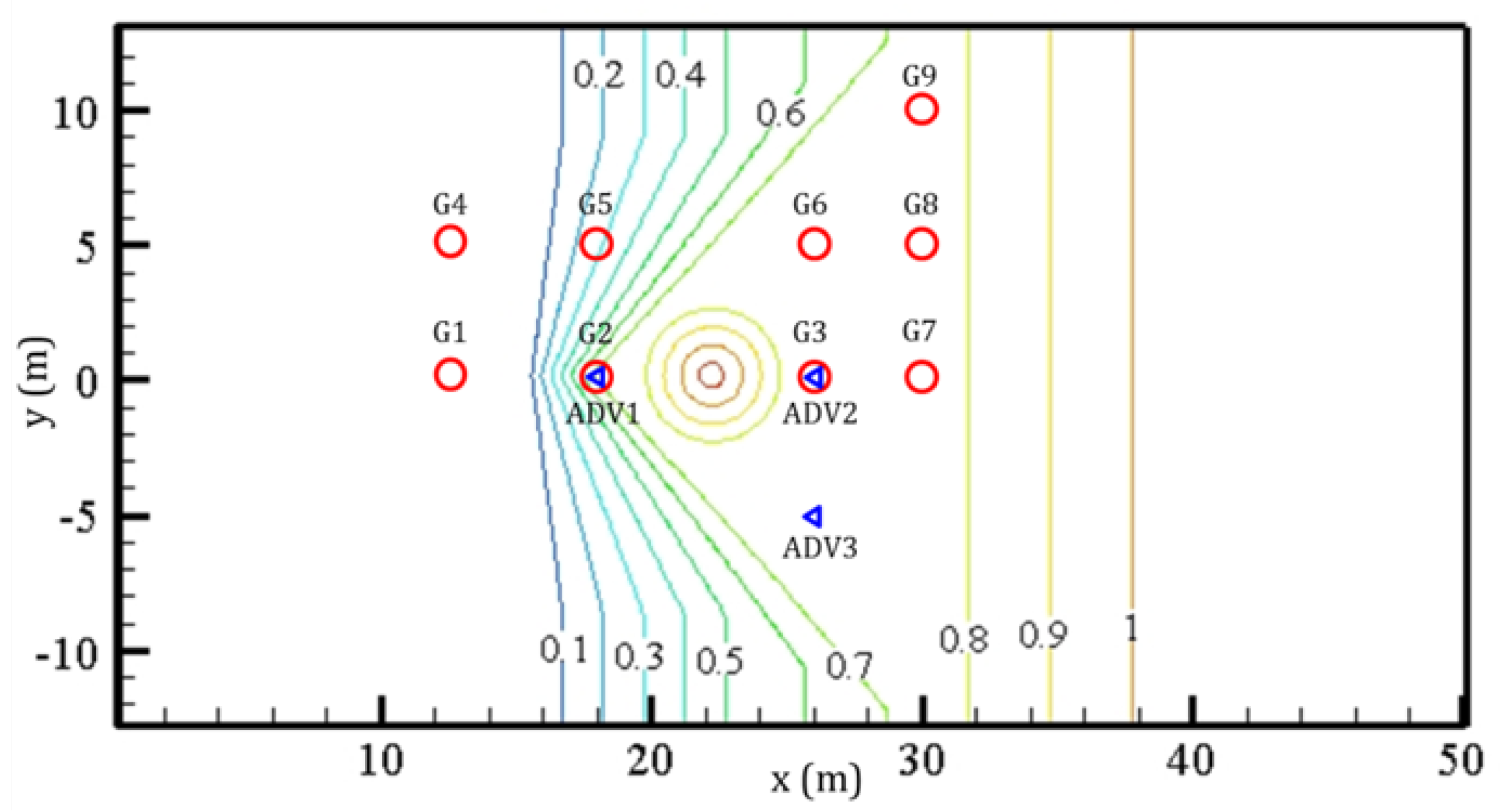
In this section, the simulated case aims to test the model’s capability on simulating solitary wave breaking, runup and rundown over a three-dimensional complex bathymetry, which consists of a 1:30 slope, a triangular shaped shelf with a conical island located at the offshore point of the shelf as shown in Figure 13 and Figure 14. Laboratory experiments were conducted in a $48.8\mathrm{m}$ long, $26.5\mathrm{m}$ wide and $2.1\mathrm{m}$ deep wave basin [38]. A piston-type wave maker generates a solitary wave from the left side in Figure 13, and the other three sides are wall. In the entire wave basin, there are nine wave gauges (G1-G9) used to measure free surface elevation and three acoustic Doppler Velocimeters (ADV1-ADV3) adopted to provide velocity data, as shown in Figure 14.

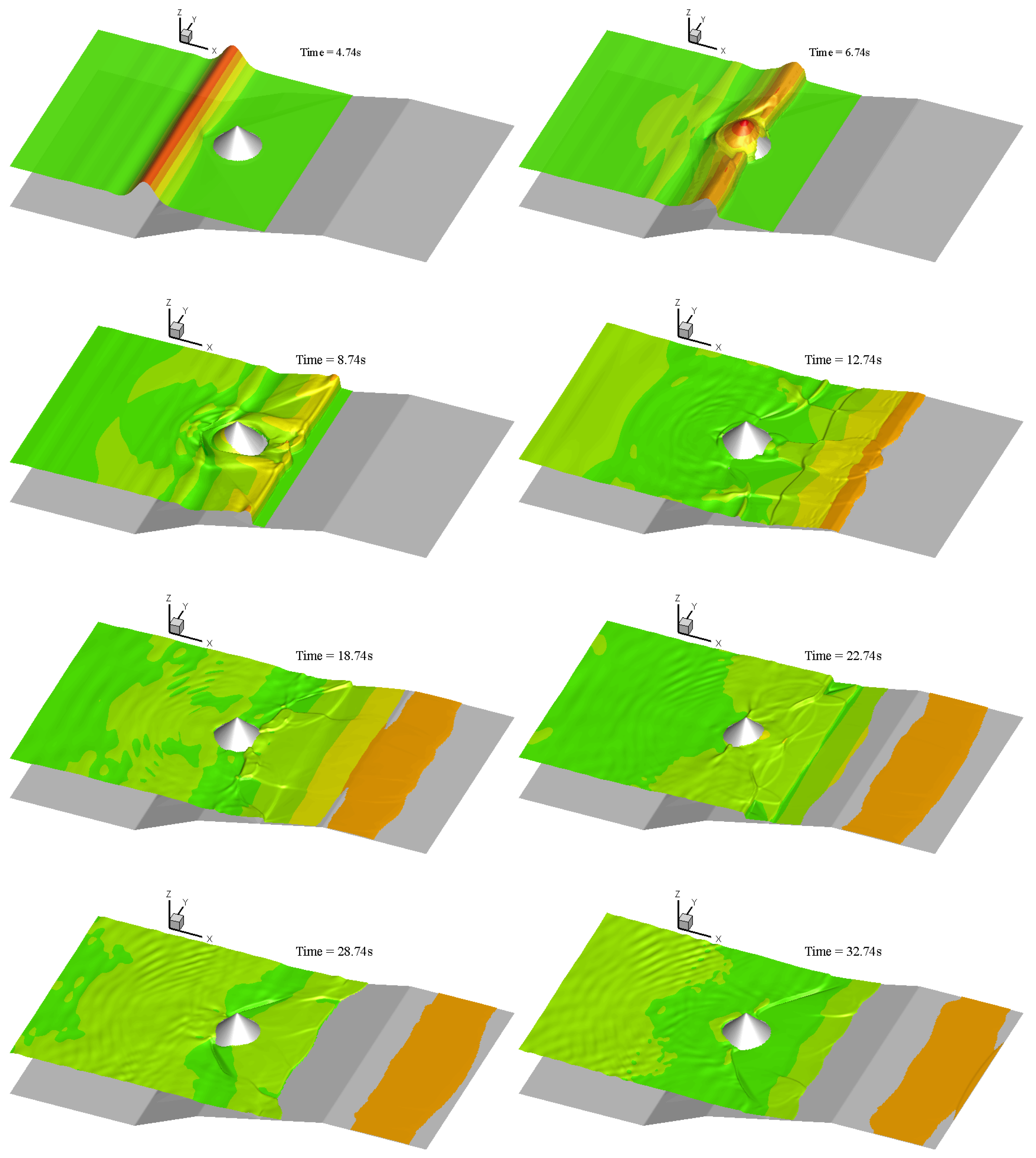
The water depth in the basin is kept constant at $0.78\mathrm{m}$, and the incident wave height is $0.39\mathrm{m}$. The computational domain includes $500\times 260$ rectangular cells ($\Delta x=\Delta y=0.1\mathrm{m}$), and the Manning’s coefficient is assigned as $0.014\mathrm{s}/{\mathrm{m}}^{1/3}$. Figure 15 shows the water level fluctuations over the entire domain at different times. As seen in Figure 15, the solitary wave propagates from the left side to the right side. At $t=5\mathrm{s}$, the wave encounters triangular-shaped shelf and begins to climb on the shelf. When $t=6.75\mathrm{s}$, the wave passes over the conical island, the shoaling effect causes the wave to become asymmetric, and then the wave breaking occurs. After the wave breaking, the wave keeps climbing over the shelf, reaches the right boundary, and then reflects back at $t=29\mathrm{s}$.

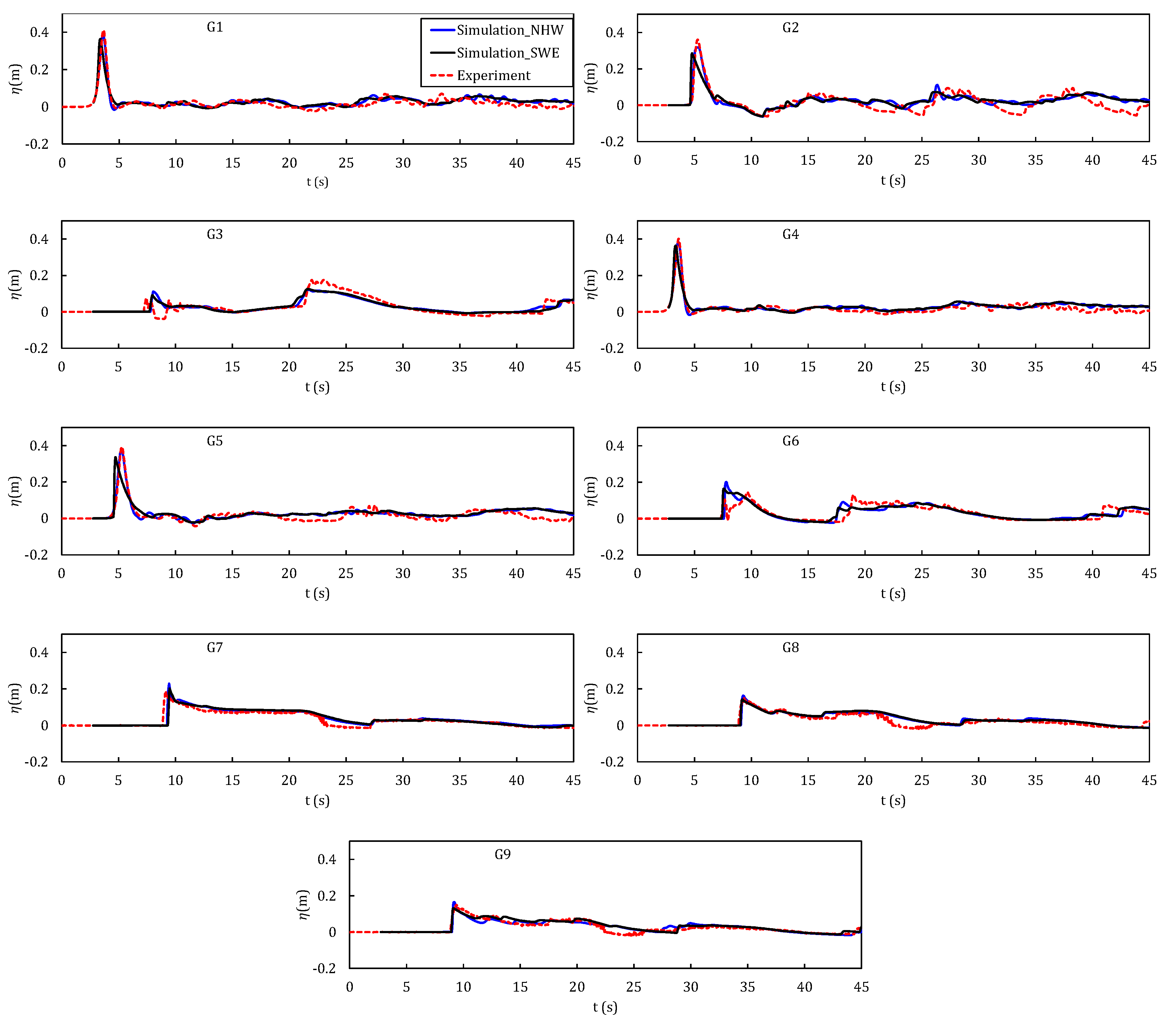
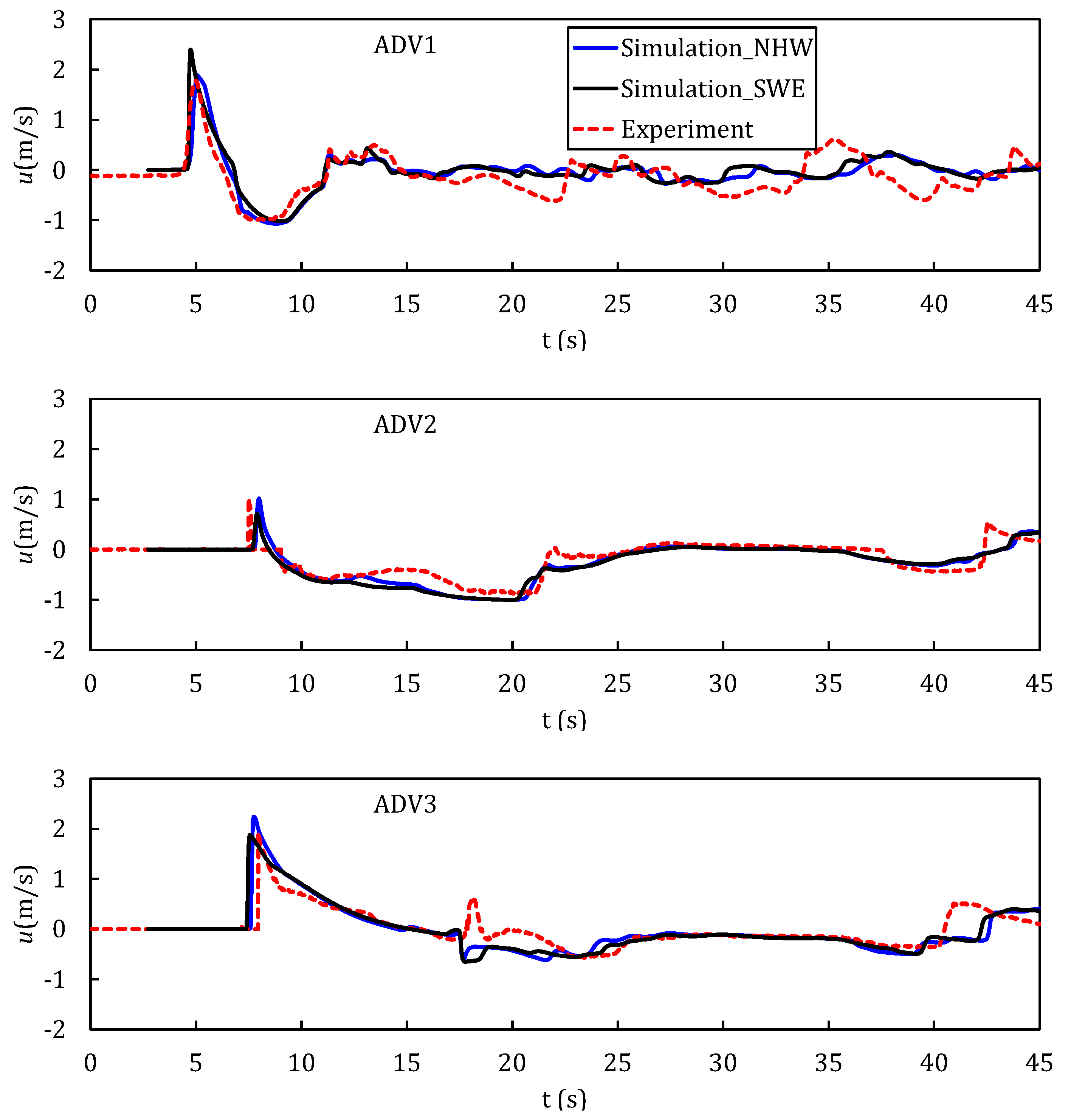
Figure 16 presents the simulated water level using the NHW and SWE model, respectively. For G1, G2, G4, and G5 stations, the wave amplitude calculated by the SWE model is lower than the experimental results. By considering the wave dispersion effects, the NHW model could simulate wave amplitudes more accurately and simulated results agree with the measurement fairly well. For G3 and G6 stations, there are certain deviations between the simulations and measurements, which also exist in other studies [19,20,21]. For G7, G8, and G9 stations (near the side wall), the simulations are fairly close to the measurements, which implies that the model can also accurately simulate the wave reflection from the side wall regions. Figure 17 performs the temporal velocity variations at the x direction for three velocity measurement stations using NHW and SWE model, respectively. Both the NHW and SWE model can capture most of the features of the velocities at ADV1-ADV3. In general, the developed NHW model exhibits reasonable agreement with the measurements of the solitary wave propagating over a three-dimensional complex bathymetry. The source code of the model, which is compiled with the Visual Studio 2008 and C++ language, executed on a single CPU core. The CPU time is about $2.015\mathrm{h}$ on a desktop computer with Intel i5-3470 CPU 3.2 GHz, 8 GB memory.

4. Conclusions

In this study, a two-dimensional depth-integrated non-hydrostatic wave model is developed. The model solves the governing equations with hydrostatic and non-hydrostatic pressure separately. To obtain the velocities under hydrostatic pressure conditions, the finite volume method with central-upwind scheme is adopted. For including the non-hydrostatic effect, the biconjugate gradient stabilized method is adopted to solve the non-hydrostatic pressure, and then the velocities can be corrected. The HFA method is used to deal with the wave breaking issue, and after the wave breaks, the non-hydrostatic model is transformed into the hydrostatic shallow water model, where the non-hydrostatic pressure and vertical velocity are set to zero.

Several analytical solutions and laboratory experiments are used to verify the accuracy and robustness of the developed model. In general, the numerical simulations are in good agreement with the theoretical or experimental results, which indicates that the model can be used to simulate large-scale wave motions in practical engineering applications. This model can only be used for the calculation of weakly nonlinear and dispersive waves, while for the simulation of highly nonlinear and dispersive waves, a multi-layer (three-dimensional) non-hydrostatic model is needed, which is our future work.

References

- Peregrine, D.H. Long waves on a beach. J. Fluid Mech. 1967, 27, 815–827. [Google Scholar] [CrossRef]
- Madsen, P.A.; Murray, R.; Sørensen, O.R. A new form of the Boussinesq equations with improved linear dispersion characteristics. Coast. Eng. 1991, 15, 371–388. [Google Scholar] [CrossRef]
- Madsen, P.A.; Bingham, H.; Schäffer, H. Boussinesq-type formulations for fully nonlinear and extremely dispersive water waves: Derivation and analysis. Proc. R. Soc. Lond. Ser. A Math. Phys. Eng. Sci. 2003, 459, 1075–1104. [Google Scholar] [CrossRef]
- Nwogu, O. Alternative form of Boussinesq equations for nearshore wave propagation. J. Waterw. Port Coast. Ocean Eng. 1993, 119, 618–638. [Google Scholar] [CrossRef] [Green Version]
- Wei, G.; Kirby, J.T.; Grilli, S.T.; Subramanya, R. A fully nonlinear Boussinesq model for surface waves. Part 1. Highly nonlinear unsteady waves. J. Fluid Mech. 1995, 294, 71–92. [Google Scholar] [CrossRef]
- Kennedy, A.B.; Chen, Q.; Kirby, J.T.; Dalrymple, R.A. Boussinesq modeling of wave transformation, breaking, and runup. I: 1D. J. Waterw. Port Coast. Ocean Eng. 2000, 126, 39–47. [Google Scholar] [CrossRef] [Green Version]
- Kirby, J.T. Boussinesq Models and Their Application to Coastal Processes across a Wide Range of Scales. Ph.D. Thesis, American Society of Civil Engineers, Reston, VA, USA, 2016. [Google Scholar]
- Yamazaki, Y.; Kowalik, Z.; Cheung, K.F. Depth-integrated, non-hydrostatic model for wave breaking and run-up. Int. J. Numer. Methods Fluids 2009, 61, 473–497. [Google Scholar] [CrossRef]
- Stelling, G.; Zijlema, M. An accurate and efficient finite-difference algorithm for non-hydrostatic free-surface flow with application to wave propagation. Int. J. Numer. Methods Fluids 2003, 43, 1–23. [Google Scholar] [CrossRef]
- Wei, Z.; Jia, Y. A depth-integrated non-hydrostatic finite element model for wave propagation. Int. J. Numer. Methods Fluids 2013, 73, 976–1000. [Google Scholar] [CrossRef]
- Li, B.; Fleming, C.A. Three-dimensional model of Navier-Stokes equations for water waves. J. Waterw. Port Coast. Ocean Eng. 2001, 127, 16–25. [Google Scholar] [CrossRef]
- Harlow, F.H.; Welch, J.E. Numerical calculation of time-dependent viscous incompressible flow of fluid with free surface. Phys. Fluids 1965, 8, 2182–2189. [Google Scholar] [CrossRef]
- Hirt, C.W.; Nichols, B.D. Volume of fluid (VOF) method for the dynamics of free boundaries. J. Comput. Phys. 1981, 39, 201–225. [Google Scholar] [CrossRef]
- Christensen, E.D.; Deigaard, R. Large eddy simulation of breaking waves. Coast. Eng. 2001, 42, 53–86. [Google Scholar] [CrossRef]
- Lara, J.; Garcia, N.; Losada, I. RANS modelling applied to random wave interaction with submerged permeable structures. Coast. Eng. 2006, 53, 395–417. [Google Scholar] [CrossRef]
- Zijlema, M.; Stelling, G.; Smit, P. SWASH: An operational public domain code for simulating wave fields and rapidly varied flows in coastal waters. Coast. Eng. 2011, 58, 992–1012. [Google Scholar] [CrossRef]
- Ma, G.; Shi, F.; Kirby, J.T. Shock-capturing non-hydrostatic model for fully dispersive surface wave processes. Ocean Model. 2012, 43, 22–35. [Google Scholar] [CrossRef]
- Pan, W.; Kramer, S.C.; Piggott, M.D. Multi-layer non-hydrostatic free surface modelling using the discontinuous Galerkin method. Ocean Model. 2019, 134, 68–83. [Google Scholar] [CrossRef]
- Wei, Z.; Jia, Y. Simulation of nearshore wave processes by a depth-integrated non-hydrostatic finite element model. Coast. Eng. 2014, 83, 93–107. [Google Scholar] [CrossRef]
- Lu, X.; Dong, B.; Mao, B.; Zhang, X. A two-dimensional depth-integrated non-hydrostatic numerical model for nearshore wave propagation. Ocean Model. 2015, 96, 187–202. [Google Scholar] [CrossRef]
- Fang, K.; Liu, Z.; Zou, Z. Modelling coastal water waves using a depth-integrated, non-hydrostatic model with shock-capturing ability. J. Hydraul. Res. 2015, 53, 119–133. [Google Scholar] [CrossRef]
- Aricò, C.; Re, C.L. A non-hydrostatic pressure distribution solver for the nonlinear shallow water equations over irregular topography. Adv. Water Resour. 2016, 98, 47–69. [Google Scholar] [CrossRef] [Green Version]
- Ginting, B.M.; Ginting, H. Extension of artificial viscosity technique for solving 2D non-hydrostatic shallow water equations. Eur. J. Mech. B Fluids 2020, 80, 92–111. [Google Scholar] [CrossRef]
- Friedrichs, K.O. Symmetric hyperbolic linear differential equations. Commun. Pure Appl. Math. 1954, 7, 345–392. [Google Scholar] [CrossRef]
- Lax, P.D. Weak solutions of nonlinear hyperbolic equations and their numerical computation. Commun. Pure Appl. Math. 1954, 7, 159–193. [Google Scholar] [CrossRef]
- Nessyahu, H.; Tadmor, E. Non-oscillatory central differencing for hyperbolic conservation laws. J. Comput. Phys. 1990, 87, 408–463. [Google Scholar] [CrossRef] [Green Version]
- Kurganov, A.; Tadmor, E. New high-resolution central schemes for nonlinear conservation laws and convection–diffusion equations. J. Comput. Phys. 2000, 160, 241–282. [Google Scholar] [CrossRef] [Green Version]
- Ginting, B.M.; Mundani, R.P. Comparison of Shallow Water Solvers: Applications for Dam-Break and Tsunami Cases with Reordering Strategy for Efficient Vectorization on Modern Hardware. Water 2019, 11, 639. [Google Scholar] [CrossRef] [Green Version]
- Wu, G.F.; He, Z.G.; Zhao, L.; Liu, G.H. A well-balanced positivity preserving two-dimensional shallow flow model with wetting and drying fronts over irregular topography. J. Hydrodyn. 2018, 30, 618–631. [Google Scholar] [CrossRef]
- Liang, Q. Flood simulation using a well-balanced shallow flow model. J. Hydraul. Eng. 2010, 136, 669–675. [Google Scholar] [CrossRef]
- Larsen, J.; Dancy, H. Open boundaries in short wave simulations—A new approach. Coast. Eng. 1983, 7, 285–297. [Google Scholar] [CrossRef] [Green Version]
- Chen, Q.; Madsen, P.A.; Basco, D.R. Current effects on nonlinear interactions of shallow-water waves. J. Waterw. Port Coast. Ocean Eng. 1999, 125, 176–186. [Google Scholar] [CrossRef]
- Smit, P.; Zijlema, M.; Stelling, G. Depth-induced wave breaking in a non-hydrostatic, near-shore wave model. Coast. Eng. 2013, 76, 1–16. [Google Scholar] [CrossRef]
- Synolakis, C.E. The runup of solitary waves. J. Fluid Mech. 1987, 185, 523–545. [Google Scholar] [CrossRef]
- Roeber, V.; Cheung, K.F. Boussinesq-type model for energetic breaking waves in fringing reef environments. Coast. Eng. 2012, 70, 1–20. [Google Scholar] [CrossRef]
- Kazolea, M.; Delis, A.I.; Synolakis, C.E. Numerical treatment of wave breaking on unstructured finite volume approximations for extended Boussinesq-type equations. J. Comput. Phys. 2014, 271, 281–305. [Google Scholar] [CrossRef]
- Briggs, M.J.; Synolakis, C.E.; Harkins, G.S.; Green, D.R. Laboratory experiments of tsunami runup on a circular island. Pure Appl. Geophys. 1995, 144, 569–593. [Google Scholar] [CrossRef]
- Swigler, D.T. Laboratory Study Investigating the Three-Dimensional Turbulence and Kinematic Properties Associated with a Breaking Solitary Wave. Ph.D. Thesis, Texas A & M University, Uvalde, TX, USA, 2010. [Google Scholar]
- Kurganov, A.; Petrova, G. A second-order well-balanced positivity preserving central-upwind scheme for the Saint-Venant system. Commun. Math. Sci. 2007, 5, 133–160. [Google Scholar] [CrossRef] [Green Version]
- Audusse, E.; Bouchut, F.; Bristeau, M.O.; Klein, R.; Perthame, B.T. A fast and stable well-balanced scheme with hydrostatic reconstruction for shallow water flows. SIAM J. Sci. Comput. 2004, 25, 2050–2065. [Google Scholar] [CrossRef]
Figure 1.
Sketch of the computational domain.
Figure 2.
Two-dimensional finite-volume mesh.
Figure 3.
Comparisons between simulated results and analytic solutions at , 25 and for solitary wave propagation in constant depth.
Figure 4.
L2 error norms in as function of for solitary wave propagation in constant depth.
Figure 5.
The experimental set-up for a solitary wave climbing up a sloping beach.
Figure 6.
Comparisons of results from shallow water equation (SWE), non-hydrostatic wave model (NHW) models and measurements at different times for breaking solitary wave runup and rundown.
Figure 7.
The experimental setup and bottom geometry for propagation of solitary wave over fringing reef.
Figure 8.
Comparisons between simulated and experimental surface elevations for propagation of solitary wave over fringing reef.
Figure 9.
Comparison of simulated and measured time series free surface elevations for a solitary wave propagation over an exposed reef crest.
Figure 10.
The experimental setup and bottom geometry for runup of a solitary wave on a circular island (Note: Red dots denote wave gauges).
Figure 11.
Comparisons of numerical simulation and experiments for runup of a solitary wave on a circular island. The first column is the relative wave height at condition ; the second column is the relative wave height at condition ; the third column is the relative wave height at condition .
Figure 12.
Comparisons of the maximum wave runup between the simulation and measurement for runup of a solitary wave on a circular island. Left, middle, right panels represent the relative wave height at condition , , and , respectively.
Figure 13.
The geometry in Swigler’s (2009) experiments.
Figure 14.
Contours and locations of measuring points (“circle” symbols are the gauges for water surface fluctuation measurement, and “triangle” symbols are the acoustic Doppler Velocimeters (ADVs) for velocity measurement).
Figure 15.
Water level fluctuations at different times for breaking and runup of a solitary wave over a three-dimensional complex bathymetry.
Figure 16.
Comparisons of temporal water level fluctuations at different gauge stations.
Figure 17.
Comparisons of temporal velocity variations at the x direction for breaking and runup of a solitary wave over a three-dimensional complex bathymetry.
© 2020 by the authors. Licensee MDPI, Basel, Switzerland. This article is an open access article distributed under the terms and conditions of the Creative Commons Attribution (CC BY) license (http://creativecommons.org/licenses/by/4.0/).
Share and Cite
MDPI and ACS Style
Wu, G.; Lin, Y.-T.; Dong, P.; Zhang, K. Development of Two-Dimensional Non-Hydrostatic Wave Model Based on Central-Upwind Scheme. J. Mar. Sci. Eng. 2020, 8, 505. https://doi.org/10.3390/jmse8070505
AMA Style
Wu G, Lin Y-T, Dong P, Zhang K. Development of Two-Dimensional Non-Hydrostatic Wave Model Based on Central-Upwind Scheme. Journal of Marine Science and Engineering. 2020; 8(7):505. https://doi.org/10.3390/jmse8070505
Chicago/Turabian StyleWu, Gangfeng, Ying-Tien Lin, Ping Dong, and Kefeng Zhang. 2020. "Development of Two-Dimensional Non-Hydrostatic Wave Model Based on Central-Upwind Scheme" Journal of Marine Science and Engineering 8, no. 7: 505. https://doi.org/10.3390/jmse8070505
Note that from the first issue of 2016, this journal uses article numbers instead of page numbers. See further details here.