Real-Time Processing and High-Quality Imaging of Navigation Strip Data Using SSS Based on AUVs

Abstract

In light of the prevailing approach in which data from side-scan sonar (SSS) from Autonomous Underwater Vehicles (AUVs) are primarily processed and visualized post mission, failing to meet the requirements in terms of timeliness for on-the-fly image acquisition, this paper introduces a novel method for real-time processing and superior imaging of navigation strip data from SSS aboard AUVs. Initially, a comprehensive description of the real-time processing sequence is provided, encompassing the integration of multi-source navigation data using Kalman filtering, and high-pass filtering of attitude and heading data to exclude anomalies, as well as the use of bidirectional filtering techniques within and between pings, ensuring real-time quality control of raw data. In addition, this study adopts the semantic segmentation Unet network for automatic real-time tracking of seafloor lines, devises a real-time correction strategy for radial distortion based on historical echo data, and utilizes the alternating direction multiplier method for real-time noise reduction in strip images. With the combined application of these four pivotal techniques, we adeptly address the primary challenges in real-time navigation data processing. In conclusion, marine tests conducted in Bohai Bay substantiate the efficacy of the methodologies delineated in this research, offering a fresh paradigm for real-time processing and superior visualization of SSS navigation strip data on AUVs.

1. Introduction

SSS obtains high-resolution sonar images via line scanning, primarily for underwater target detection and seabed topography surveys [1,2,3]. Traditionally, SSS operation has primarily been carried out by mother ships equipped with SSS equipment [4,5], employing a towed approach. However, this method cannot deeply penetrate sensitive and remote areas for task execution, thus greatly restricting its operational scope.

In recent years, AUVs, with their long range and high autonomy, have been assigned tasks in sensitive, remote waters [6]. Furthermore, due to their deep submergence capacity and strong attitude control characteristics, AUVs can provide a stable platform for SSS, reducing the distance between the transducer and the seabed, thus enhancing the resolution of the data [7,8]. Therefore, AUV-mounted SSS shows broad application prospects in areas such as underwater target detection, seabed topographic mapping, underwater cruise warning, underwater matched navigation, and more. However, due to the limitations of underwater acoustic communication, large amounts of SSS data can only be processed after the AUV has been recovered, thus failing to meet the need for real-time image acquisition and processing for navigation strip data [9]. In certain critical missions, such as real-time detection and identification of specific underwater obstacles or potential targets, there may be a need for an AUV to perform real-time strip data processing and imaging based on the data collected by its side-scan sonar. Such real-time processing can provide timely information feedback for the AUV navigation and decision making. Therefore, there is an urgent need for research on real-time processing and high-quality imaging based on SSS navigation strip data obtained from AUVs.

For clarity, the term “strip” typically refers to the sonar data of each ping from the side-scan sonar. In addition, “navigation strip data using SSS” refers to the data collected by the side-scan sonar system on an AUV during its voyage on a ping-by-ping basis.

Traditional post-processing of SSS strip data includes decoding of the original binary observation files and extraction of raw data, quality control of raw observation data, generation of strip waterfall images, tracking of seabed lines, correction of radiation distortion, slant range correction, image denoising, and geographic coding [10,11]. Due to the complexity of the marine water and seabed environments, raw SSS data can be severely affected by noise and other factors, exhibiting issues like radiation distortion and geometric distortion, severely affecting the effects of SSS data processing and the quality of imaging, reducing the reliability of tasks such as underwater target detection, underwater matched navigation, and so on [12,13]. To enhance the quality of SSS images, many scholars have conducted a considerable amount of research [14,15,16,17].

For example, Zhao et al. [18] considered the continuous change and symmetric distribution of the seabed line and proposed a comprehensive seabed line tracking method that was still able to achieve robust tracking results in complex measurement environments. Wang Xiao [19] analyzed the characteristics of the SSS waterfall image and proposed a seabed line threshold tracking method. Wang et al. [20] proposed a seabed line extraction method in consideration of the spatial distribution characteristics of the seabed line. This method consists of two steps: point density clustering and chain search, and has strong anti-interference ability in complex measurement environments. Wang Aixue [21], based on the distribution characteristics of echo intensity in time and space, proposed a strip image equalization method based on statistical parameters. Buscombe [22] achieved the correction of radiation distortion of lightweight SSS echo images based on a simplified model of shallow-sea sonar-target geometry, acoustic backscatter, and sound wave attenuation, promoting the popularization and application of lightweight SSS systems in seabed habitat surveys. Shih et al. [23] proposed a seabed line tracking method combining image filtering, image segmentation, and edge detection techniques, achieving high accuracy. Although the aforementioned methods have improved the quality of SSS strip images to a certain extent, they are all post-processing methods and are not applicable to real-time processing, and cannot meet the needs of real-time processing and high-quality imaging of navigation strip data mounted on AUVs.

In summary, the main approach for handling data obtained from AUV-mounted SSS is post-processing and imaging, which does not satisfy the requirements of the real-time detection of targets or the in-transit acquisition of seabed topography images [24,25]. Hence, this paper studies the real-time processing and high-quality imaging of SSS navigation strip data based on AUVs. The structure of this paper is as follows:

Firstly, we introduce the research background and related work, clarifying the uniqueness and necessity of this study. Subsequently, the research methodologies and strategies are detailed. Based on this foundation, the major contributions of our study can be summarized as follows:

• We construct and analyze a real-time processing flow, addressing the limitations of existing post-processing strategies when applied in real-time contexts.
• A comprehensive real-time data quality management strategy is introduced, providing methods for optimizing key data and performing efficient filtering.
• Utilizing a strategy based on the Unet network, we achieve heightened efficiency and accuracy in automatic seafloor line tracking.
• Innovatively, we propose the use of statistical characteristics from historical echo data for real-time correction of radial distortion.
• We introduce a technique based on the Alternating Direction Multiplier Method, offering a novel approach to real-time noise reduction for strip images.
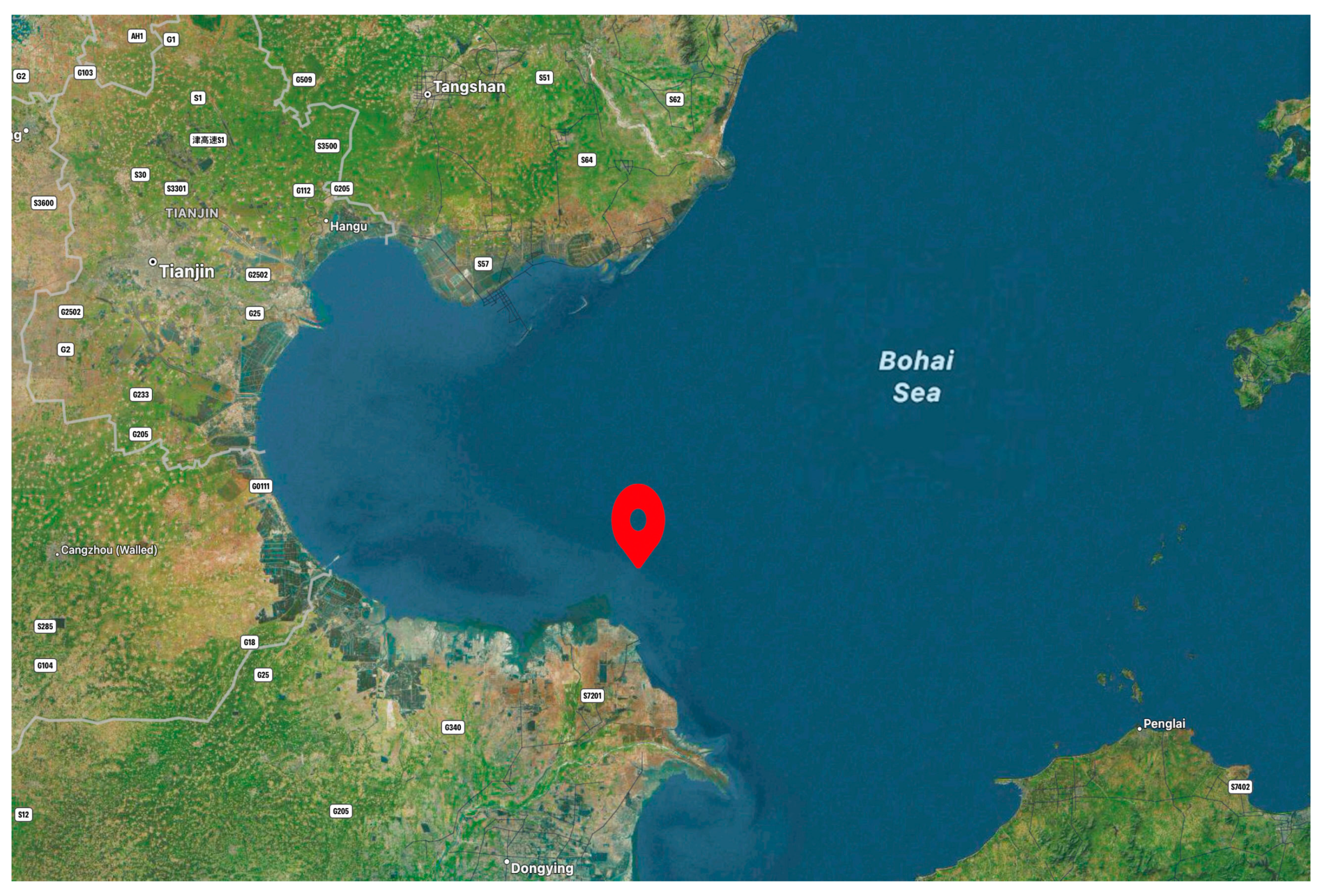
• Through on-site experiments in Bohai Bay, the robustness and practicality of our proposed methods are thoroughly validated.

The conclusion of the article analyzes the experimental results, providing a summary and recommendations.

2. Key Technologies for Real-Time Processing and High-Quality Imaging of the Navigational Strip

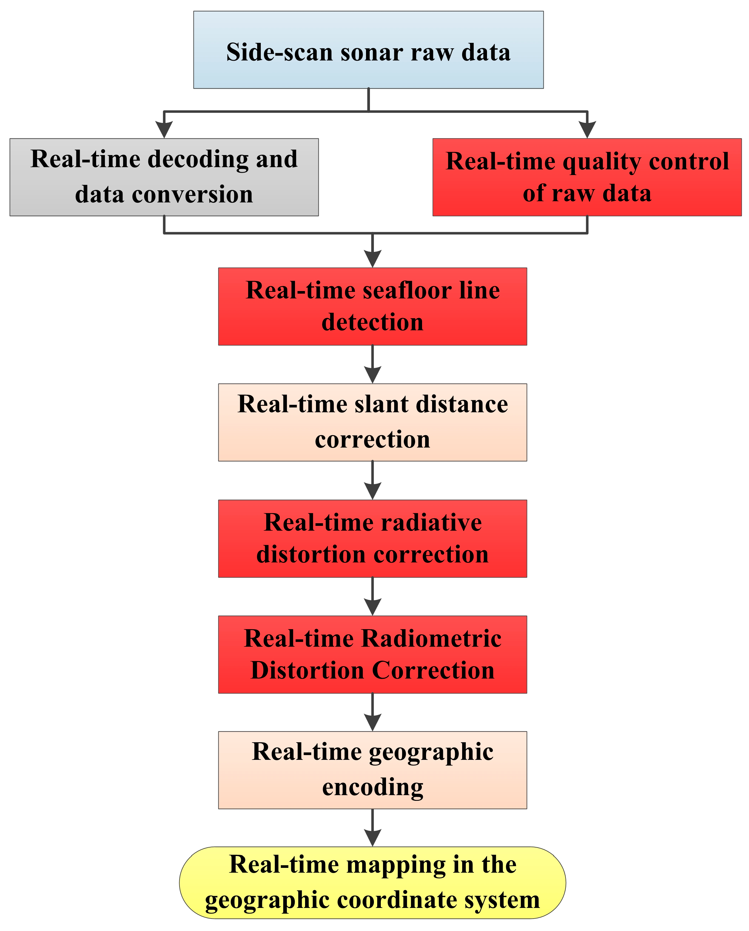
2.1. SSS Data Real-Time Processing Workflow and Existing Problems

For common tasks such as obtaining underwater topographic images, post-processing is fully able to meet the requirements of navigational strip image acquisition [26,27]. For special tasks, however, like real-time underwater target detection by AUVs, post-processing evidently fails to satisfy the need for real-time acquisition of in situ SSS images [28]. Accordingly, based on the actual circumstances of underwater navigational strip data acquisition by AUVs, a workflow for real-time processing of SSS data is proposed, as shown in Figure 1.

Figure 1 presents a flowchart of real-time processing of SSS data, where the specific process includes real-time decoding and conversion of the raw data, quality control, seafloor line tracking [29], slant range correction, radial distortion correction, noise reduction, and geographical coding and mapping. This procedure is similar to the post-processing flow, but it must be conducted in real-time while the AUV is operating, ensuring that the data for each ping are directly and effectively processed, rather than waiting for the line data for the entire survey to be fully collected in order to perform post-processing.

It is important to emphasize that in this section, our definition of “real time” refers to processing the SSS data on a per-ping basis, in contrast than the traditional method of processing an entire survey line. In real-time data processing, certain areas need to be addressed due to their challenges with respect to real-time processing.

(1)

Real-Time Quality Control of Raw Observation Data

As this is dynamic measurement, navigation data obtained using the navigation and positioning system mounted on the AUV (comprising INS, DVL, pressure sensors, etc.), echo intensity data on the real-time scan line obtained by the SSS system, etc., present problems due to the multiple data types involved and the large data volume. In post-processing, these raw observational data are often filtered using manual intervention, manual thresholds, or automatic filtering methods. For automatic filtering, unlike post-processing, real-time data series only include previous observation values, and do not incorporate subsequent observation information, and it is impossible to set a threshold manually according to data quality. Thus, existing post-processing filtering methods are not applicable.

(2)

Seabed Line Tracking

In post-processing, seabed line tracking is mainly performed by adopting the threshold method, and the threshold needs to be set based on human experience [14,15,16]. Obviously, the manual threshold method is not able to meet the needs of real-time processing, and a new automatic seabed line detection method needs to be established.

(3)

Radiant Distortion Correction

In post-processing methods, radiant distortion correction is achieved by calculating the base value in a local window of d × l, and then converting the gray value of the d-wide along-track sequence to the base value through a proportionality constant. This algorithm considers the problem of grayscale consistency in the local window, but does not take into account the variation in the grayscale base value of the entire strip. The determination of the grayscale base value of the entire strip can only be performed after obtaining the entire strip image, so real-time radiant distortion correction cannot be achieved.

(4)

Real-Time Denoising of Navigational Strip Images

The SSS system is a high-resolution imaging system, with the number of echoes received by a single ping reaching tens of thousands, and a pulse repetition frequency of 10~20 Hz. The resulting volume of navigational strip data is very high. Based on median and mean filtering methods commonly used in post-processing [30,31,32], full image traversal for filtering will undoubtedly consume a considerable amount of time, making it difficult to meet the real-time denoising needs of navigational strip images.

2.2. Key Technology Research

2.2.1. Real-Time Quality Control of Raw Data

The original data observed by SSS mainly include echo intensity data and data from navigation, attitude, DVL, depth gauge, and pressure gauge, etc. Real-time preprocessing and filtering are applied to these data to obtain high-quality raw observation information.

Echo Intensity Data Filtering

Echo intensity is one of the main parameters observed by the SSS system and is the basis for forming navigational strip images, so it is crucial to ensure its quality. Assuming the changes in seabed sediments and topography are uniform within a single ping swath, the echo intensity of a single ping from SSS exhibits a gradient. Based on this, a sliding filter method based on statistical characteristics is proposed within the ping sequence to eliminate the influence of abnormal echo intensities in the ping echo sequence.

Assume the echo intensity series within a ping is BS = {BS₁, BS₂, BS₃,…, BS_n}, with a set window length of m. Then, in the m-window, the real-time filter parameters are calculated using the following model.

$$\begin{array}{c}B{S}_0=\frac{1}{m}{\displaystyle \sum _{j=1}^{m}B{S}_j}\\ \mathrm{\Delta }B{S}_j=B{S}_j-B{S}_0\\ \sigma =\sqrt{\frac{{\displaystyle \sum _{j=1}^m{(B{S}_j-B{S}_0)}^2}}{m-1}}\end{array}$$

(1)

Based on the following principles, the echo intensity within the window is filtered.

$$\{\begin{array}{c}\mathrm{\Delta }B{S}_j\le 3\times \sigma \begin{array}{cc}\begin{array}{cc}& then\end{array}& retain\end{array}\\ \mathrm{\Delta }B{S}_j>3\times \sigma \begin{array}{cc}& then\end{array}\begin{array}{cc}& remove\end{array}\end{array}$$

(2)

Within the range of BS₁ to BS_n, we slide a window of length ‘m’ at intervals of m/2, conducting the filtering process within this window to eliminate the influence of abnormal echo intensities, ensuring the quality of the original echo strength. To adapt to different terrains and noise environments, we adjust the value of ‘m’ accordingly. For areas with low noise and relatively flat terrains, we recommend selecting a smaller window size, such as m = 5, for faster processing. Conversely, in noisy areas with complex terrains, a larger window size, like m = 20, is suggested to ensure more robust noise reduction and better representation of terrain variations. This guarantees the quality of the echo intensity within each ping. Similar work is carried out in multiple ping sequences formed by the same beam, ensuring the consistency of echo intensity changes along the survey track. This combination of lateral filtering (within pings) and longitudinal filtering (between pings) not only ensures that the echo intensity consistently reflects the scanning object but also further ensures the high quality of echo intensity data.

INS, DVL, Depth/Height Data Filtering

• Quality control of data provided by INS

Position and attitude data are provided by INS. After initialization, the Strapdown Inertial INS obtains the navigation information for the AUV by integrating the angular velocity and specific force information output from the Inertial Measurement Unit (IMU) using the navigation algorithm. The navigation and attitude information output by INS mainly consists of attitude updates (Roll, Pitch, Yaw), heading updates (Heading), velocity updates (v_x, v_y), and position updates (X, Y). Quality control of the INS system data mainly consists of: quality control of position and speed data, quality control of attitude data, and quality control of azimuth data.

INS can output the acceleration and the velocity of the carrier, and can obtain the AUV’s planar position via “point-azimuth” calculation.

$$\{\begin{array}{l}{X}_t=X_0+v_0\cos \left(\theta \right)\left(t-t_0\right)\\ Y_t=Y_0+v_0\sin \left(\theta \right)\left(t-t_0\right)\end{array}$$

(3)

In this equation, (X_t, Y_t) are the plane coordinates at the abnormal time t, and (X₀, Y₀) are the plane positions corresponding to the time t₀ before the appearance of abnormal values; v₀ is the speed of AUV at the time t₀; and θ is the azimuth of AUV at the time t₀.

The Kalman filter is used to fuse the acceleration, velocity, and position information in order to perform real-time position, velocity, and acceleration data filtering. The Kalman filter model for discrete linear systems is as follows:

$$\{\begin{array}{l}X\left(t\right)={\mathrm{\Phi }}_{t,t-1}X\left(t-1\right)+{\mathsf{\Gamma }}_{t,t-1}\omega \left(t-1\right)\\ Z\left(t\right)=H_{t}X\left(t\right)+\mathrm{\Delta }\left(t\right)\end{array}$$

(4)

In the above formula, X(t) represents the n-dimensional state matrix of a certain discrete linear system at time t, Φ_t,t−1 is the state transition matrix of the system, X_(t−1) represents the state matrix of the system at time t−1, Γ_t,t−1 represents the process noise input matrix of the system, and ω_(t−1) is the process noise of the system at time t−1, which generally follows a Gaussian distribution. Z(t) represents the observation value at time t, H_t is the conversion relationship between the state matrix X(t) and the observation matrix Z(t) at time t, and Δ(t) represents the observation noise of the system at time t, which generally follows a Gaussian distribution.

The Kalman filter includes two steps: time prediction and measurement update. Time prediction estimates the state X(t) at time t by combining the observation values Z(1), Z(2), …, Z(t−1) before time t. The state estimate obtained from time prediction is denoted as $\widehat{X}\left(t,t-1\right)$. The time prediction process is given by Equation (5), where $D_{\widehat{X}}\left(t,t-1\right)$ and $D_{\omega }\left(t-1\right)$ represent the prediction variance and process error variance matrix, respectively.

$$\{\begin{array}{l}\widehat{X}\left(t,t-1\right)={\mathrm{\Phi }}_{t,t-1}\widehat{X}\left(t-1\right)\\ \mathrm{\Delta }\widehat{X}\left(t,t-1\right)={\mathrm{\Phi }}_{t,t-1}\mathrm{\Delta }\widehat{X}\left(t-1\right)+{\mathsf{\Gamma }}_{t,t-1}\omega \left(t-1\right)\\ D_{\widehat{X}}\left(t,t-1\right)={\mathrm{\Phi }}_{t,t-1}{D}_{\widehat{X}}\left(t-1\right){\mathrm{\Phi }}_{t,t-1}^T+{\mathsf{\Gamma }}_{t,t-1}{D}_{\omega }\left(t-1\right){\mathsf{\Gamma }}_{t,t-1}^T\end{array}$$

(5)

The measurement update of the Kalman filter estimates the state X(t) at time t by combining the observation values Z(1), Z(2), …, Z(t−1), Z(t) at time t and its previous t−1 times. This estimate is denoted as $\widehat{X}\left(t\right)$. The measurement update process is given by Equation (6), where K_t and $V_Z\left(t,t-1\right)$ are the gain matrix and innovation matrix at time t, respectively, $\mathrm{\Delta }\widehat{X}\left(t\right)$ is the filter error, and $D_{\widehat{X}}\left(t\right)$ and $D_{\mathrm{\Delta }}\left(t\right)$ are the filter variance and observation variance, respectively.

$$\{\begin{array}{l}\widehat{X}\left(t\right)=\widehat{X}\left(t,t-1\right)+K_t{V}_Z\left(t,t-1\right)\\ K_t=D_{\widehat{X}}\left(t,t-1\right)H_t^T{\left[H_t{D}_{\widehat{X}}\left(t,t-1\right)H_t^T+D_{\mathrm{\Delta }}\left(t\right)\right]}^{-1}\\ V_Z\left(t,t-1\right)=Z\left(t\right)-H_t\widehat{X}\left(t,t-1\right)\\ \mathrm{\Delta }\widehat{X}\left(t\right)=\left(I-K_t{H}_t\right)\mathrm{\Delta }\widehat{X}\left(t,t-1\right)-K_t\mathrm{\Delta }\left(t\right)\\ D_{\widehat{X}}\left(t\right)=\left(I-K_t{H}_t\right)D_{\widehat{X}}\left(t,t-1\right){\left(I-K_t{H}_t\right)}^T+K_t{D}_{\mathrm{\Delta }}\left(t\right)K_t^T\end{array}$$

(6)

As shown in Equation (6), in the process of repairing long-term abnormal plane coordinates, the state matrix X(t) at time t is composed of the plane coordinates $\left(X_t,Y_t\right)$, motion velocity $\left(v_t^x,v_t^y\right)$, and acceleration $\left(a_t^x,a_t^y\right)$ provided by the INS system at that time. The observation matrix Z(t) at the same time is also composed of the above measurement information.

$$\{\begin{array}{l}X\left(t\right)={\left[\begin{array}{cccccc}{X}_t& Y_t& v_t^x& v_t^y& a_t^x& a_t^y\end{array}\right]}^T\\ Z\left(t\right)={\left[\begin{array}{cccccc}{X}_t& Y_t& v_t^x& v_t^y& a_t^x& a_t^y\end{array}\right]}^T\end{array}$$

(7)

where the superscript “T” represents the transpose of the matrix. The state equation of the system is given by Equation (8).

$$\{\begin{array}{l}{X}_t=X_{t-1}+v_t^x\mathrm{\Delta }t+\frac{1}{2}{a}_t^x\mathrm{\Delta }{t}^2\\ Y_t=Y_{t-1}+v_t^y\mathrm{\Delta }t+\frac{1}{2}{a}_t^y\mathrm{\Delta }{t}^2\\ v_t^x=v_{t-1}^x+a_t^x\mathrm{\Delta }t\\ v_t^y=v_{y_{t-1}}+a_t^y\mathrm{\Delta }t\end{array}$$

(8)

Based on the above equation, the state transition matrix ${\mathrm{\Phi }}_{t,t-1}$, noise input matrix ${\mathsf{\Gamma }}_{t,t-1}$ and transformation matrix H_t in Equation (9) are as follows:

$$\begin{array}{c}{\mathrm{\Phi }}_{t,t-1}=\left[\begin{array}{cccccc}1& 0& \mathrm{\Delta }t& 0& \mathrm{\Delta }{t}^2/2& 0\\ 0& 1& 0& \mathrm{\Delta }t& 0& \mathrm{\Delta }{t}^2/2\\ 0& 0& 1& 0& \mathrm{\Delta }t& 0\\ 0& 0& 0& 1& 0& \mathrm{\Delta }t\\ 0& 0& 0& 0& 1& 0\\ 0& 0& 0& 0& 0& 1\end{array}\right],\\ {\mathsf{\Gamma }}_{t,t-1}=\left[\begin{array}{cc}\mathrm{\Delta }{t}^3/6& 0\\ 0& \mathrm{\Delta }{t}^3/6\\ \mathrm{\Delta }{t}^2/2& 0\\ 0& \mathrm{\Delta }{t}^2/2\\ \mathrm{\Delta }t& 0\\ 0& \mathrm{\Delta }t\end{array}\right]\\ H_t={\left[\begin{array}{cccccc}1& 0& 0& 0& 0& 0\\ 0& 1& 0& 0& 0& 0\\ 0& 0& 1& 0& 0& 0\\ 0& 0& 0& 1& 0& 0\\ 0& 0& 0& 0& 1& 0\\ 0& 0& 0& 0& 0& 1\end{array}\right]}^T\end{array}$$

(9)

2.

Quality control of DVL system data

The DVL system provides the velocity information for the AUV during navigation. However, in practical scenarios, due to the complexities of the underwater environment and the dynamic behaviors of the AUV, such as its buoyancy adjustments and directional changes, velocity measurement deviations can occur, known as gross DVL errors. While some of these large gross DVL errors can be detected and eliminated using the constraints of AUV kinematics and information from the INS system, these errors often remain elusive and unaddressed when using low-cost INS systems.

To address this challenge, we considered using side-scan sonar images to assist in detecting and rectifying these DVL gross errors. Specifically, we employed the Scale-Invariant Feature Transform (SIFT) algorithm to detect and describe keypoints in consecutive side-scan sonar frames. The SIFT algorithm is a feature extraction method based on the scale and rotation invariance of images that is capable of extracting stable keypoints even under varying scales, rotations, and illumination conditions.

The SIFT algorithm starts by constructing the scale space of the image, identifying extremal points in this space as potential keypoints:

$$L(x,y,\sigma )=G(x,y,\sigma )\times I(x,y)$$

(10)

where L is the scale space function, G is the Gaussian function, I is the input image, and σ is the scale parameter.

After identifying the keypoints, SIFT also calculates their orientation information and generates distinct descriptors based on the gradient direction and magnitude of the pixels surrounding the keypoint.

In our application, using the SIFT algorithm allows us to extract and match keypoints from consecutive side-scan sonar frames. These keypoints provide relative motion information of the AUV, as the lateral data within a single side-scan sonar frame have a fixed spatial relationship. By comparing these matched keypoints, we can estimate their lateral movement between consecutive frames, thereby deriving the lateral velocity of the AUV. The specific operation steps of the corresponding method are given in Figure 2.

3.

Quality control of depth gauge/altimeter data

The depth gauge can provide the distance from the water body to the sea surface, and the altimeter can provide the distance from the water body to the sea floor. Both are measured using sound waves. Anomalous echoes caused by water grass, suspended matter, swimming fish schools, and complex seabed terrain may cause transducer bottom detection failure.

Continuous terrain can be used as a reference, and Kalman filtering can be used to detect and correct abnormal depth data; alternatively, based on the principle of continuous terrain changes, the sliding bottleneck method can be used to detect abnormal depth data (terrain data) in order to achieve quality control of depth gauge/altimeter data.

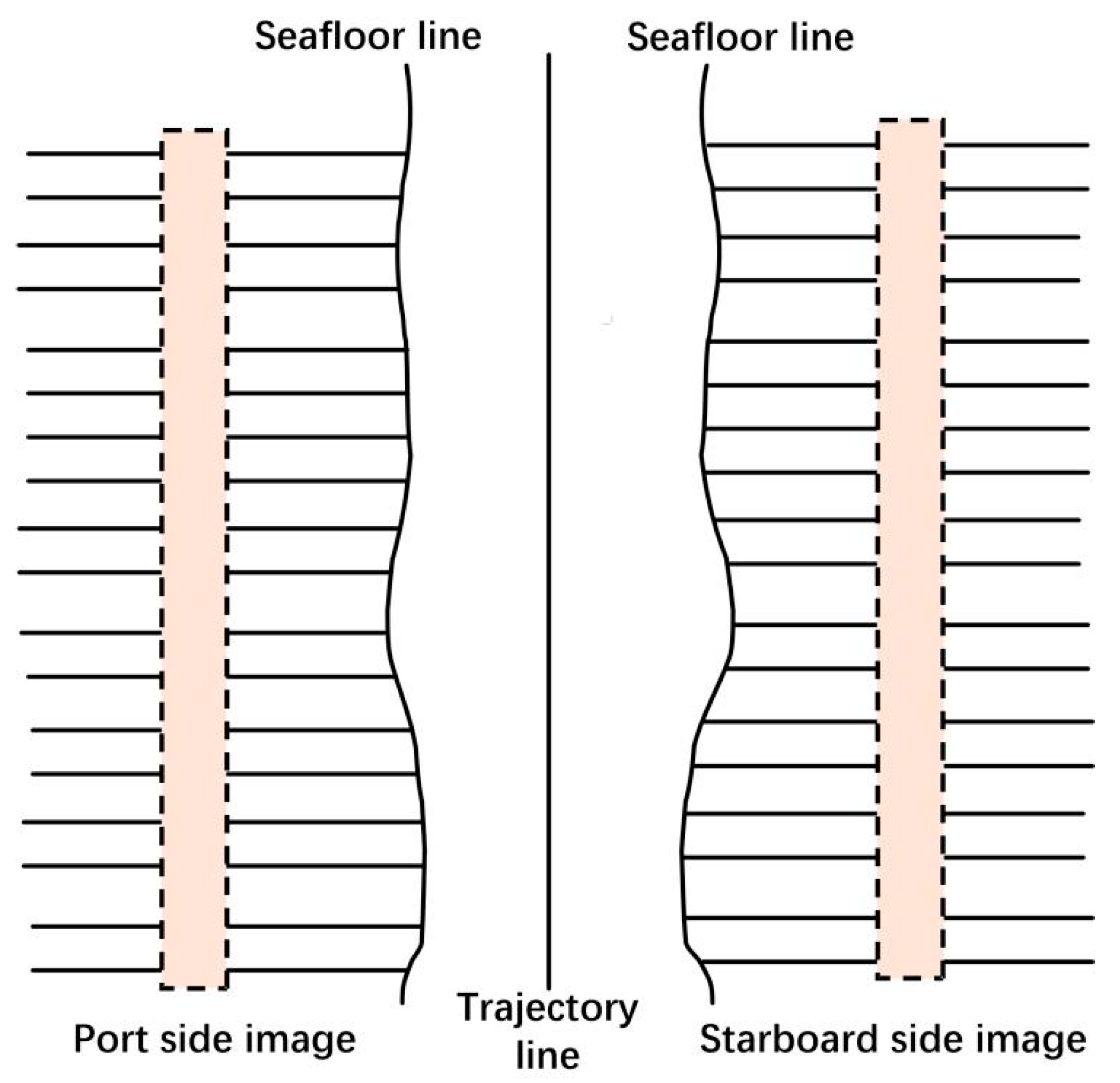
2.2.2. Real-Time Automatic Tracking of Seafloor Lines

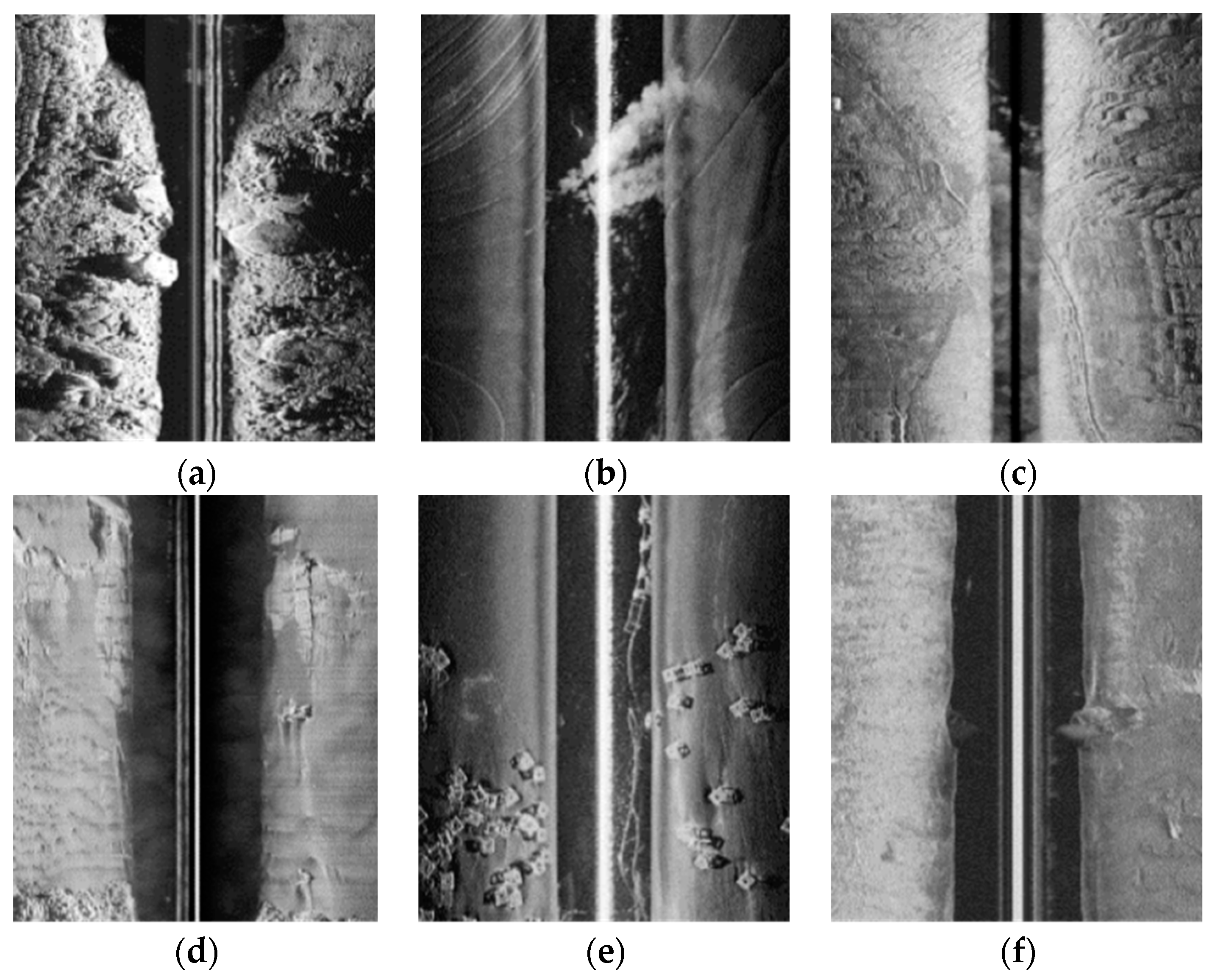
Analysis of Image Characteristics and Factors Affecting Seafloor Tracking

SSS works by emitting sound waves through transducers installed on the left and right sides. A strip image is composed of left-side scan data, central water column area, and right-side scan data. Because SSS uses slant-range imaging, severe geometric distortion occurs in the direction of the vertical track line in the original SSS waterfall image. This needs to be corrected using a series of methods, and geographic coding is performed on the basis of the corrected results. The scan data from the ship’s coordinate system are converted into the geodetic coordinate system. Accurate extraction of the SSS seafloor line is an important prerequisite for a series of subsequent operations.

In an ideal state, when sound waves propagate in water, they do not generate echoes. Only when the sound wave reaches the sea floor will it generate a strong echo. Therefore, by traversing the echo intensity sequence received by the transducer and looking for the first echo point that is greater than a preset threshold, it is easy to determine the position of the first sea bottom echo point in each piece of ping data. However, in the actual measurement process, many factors affect the accuracy of seafloor line extraction, as shown in Figure 3. The main factors impacting it are as follows:

• AUV wake

When the SSS is mounted on the hull of the AUV, the SSS will be affected by bubble turbulence or waves caused by the movement of the propeller while the AUV is traveling (causing changes in the density of the water). These bubbles produce a strong reflection of sound waves, and since the bubbles appear with the ship, they cause higher echo values within a certain range parallel to the trajectory in the waterfall chart (characterized as a grayscale peak), which can easily be misidentified as the seafloor line.

2.

Surface echo

If the backlobe beam of the transducer is not well suppressed, it will cause a part of the energy to be emitted upwards, and at a certain underwater depth, the sea level (water surface) will reflect this part of the energy, causing two strong echoes in the waterfall chart. This can also easily be misidentified as the seafloor line.

3.

Suspended matter and water quality in water

When there are suspended substances of a certain range and concentration under the SSS transducer, such as floating objects or fish schools, the beam emitted by the transducer will be reflected by the suspended substances, rendering it unable to reach the seabed surface. An echo image of the suspended substance will be formed in the waterfall chart, interfering with the accuracy of seafloor line tracking; additionally, when the water quality is poor, the reflection of sound waves by the water will be severe, resulting in complex echoes in the water column area, causing the boundary line between the water column area and the seabed to be relatively blurry.

4.

Strong absorption and contrast bottom texture

Different seabed textures have different abilities to reflect sound waves. When the seabed directly under the SSS is a bottom texture with strong absorption, most of the sound energy will be absorbed, and the first received seabed echo will be obscured by environmental noise, making it difficult to distinguish the boundary line between the seabed and the water column area, leading to a relative enlargement of the water column area. Similarly, when the seabed directly under the SSS is a bottom texture with strong reflection, the sound wave signal received by the SSS will be too strong, causing the peak of the seafloor line to be larger, and the position of the seafloor line will be biased towards the water column area, causing the water column area to shrink in relative terms. In addition, when the bottom texture directly under the SSS is very different from the side bottom texture, it will cause a relative offset of the boundary line between the bottom textures in the image, which is represented as the offset of the seafloor line in the waterfall chart, ultimately affecting the tracking accuracy of the seafloor line.

5.

Interference pulse

The SSS transducer begins to receive echoes at the moment in which the sound wave pulse is transmitted, and the interference pulse is also a signal with a very high intensity. The first signal received by the SSS transducer may be the interference signal emitted by the side lobe. Due to the short time interval between the transmission and receipt of sound waves, strong interference pulses will be generated near the zero line, and the interference pulse will also be characterized as a grayscale peak in the image, leading to incorrect seafloor line tracking.

6.

Real-time gain

In the process of data collection, in order to reduce the impact of radiation distortion on the imaging quality, data are often subjected to real-time gain. After applying gain, the energy in the water column area is more prominent, further blurring the boundary between the water column area and the seabed. In addition, the difference in quantization methods used in the process of generating waterfall charts from the original echo intensity also results in signal enhancement in the water column area, affecting the precise tracking of the seafloor line.

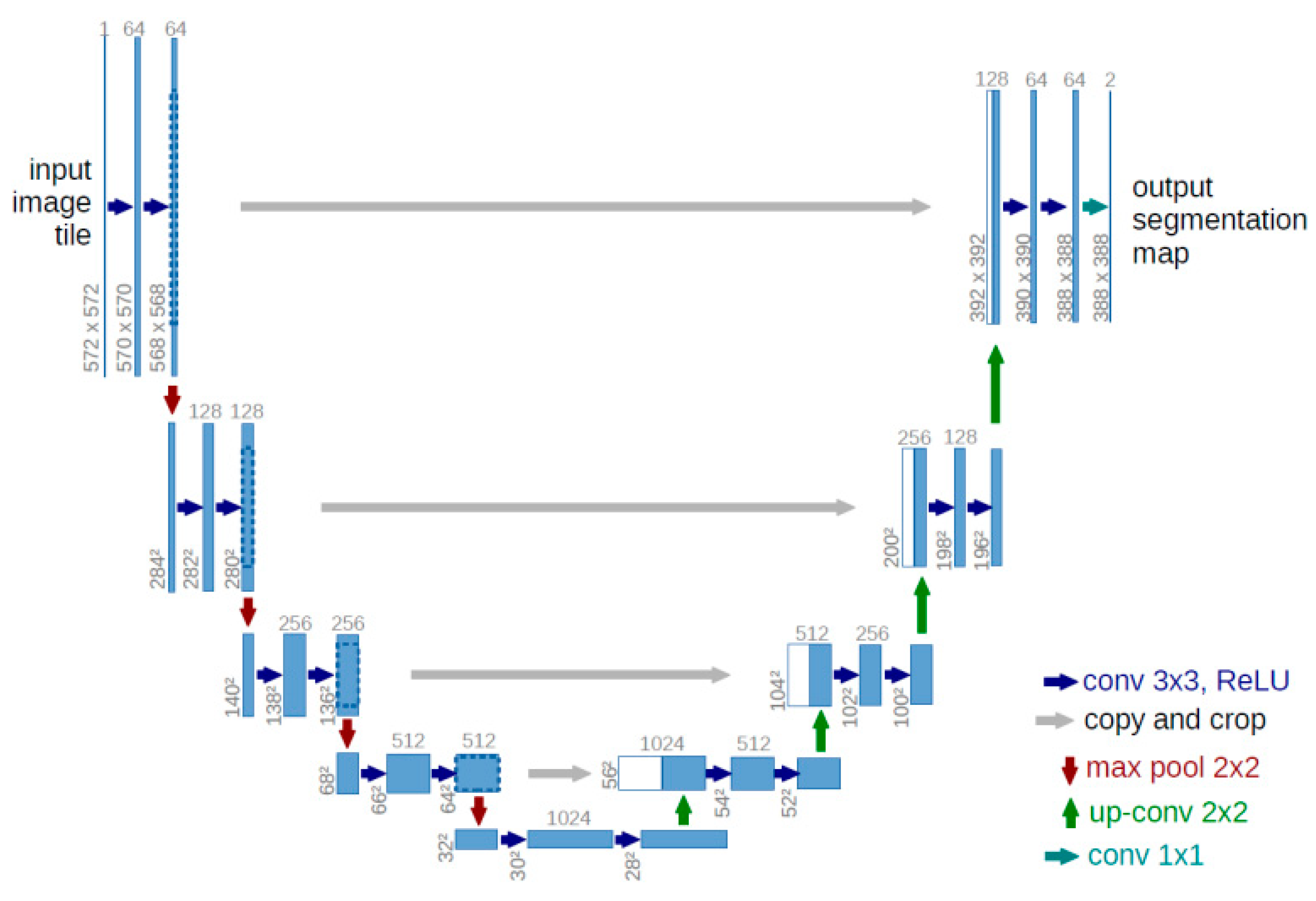
Building the Seafloor Line Semantic Segmentation Model

• Semantic segmentation model taking into consideration the symmetry of the seafloor line

Traditional seafloor line extraction methods often obtain the critical point between the seafloor and water body based on grayscale thresholds. To avoid the impact of various interference factors on seafloor line extraction, this paper uses a semantic segmentation model to segment the seafloor and water bodies.

A semantic segmentation network classifies each pixel in an image to achieve segmentation between image targets and the background area. Currently, there are many mature semantic segmentation models, and their accuracy and effectiveness have been verified on large public datasets. In order to achieve high segmentation accuracy and efficiency, the Unet network structure is introduced as the basic model, and its network structure is shown in Figure 4.

Unet consists of a contracting path (left) and an expansive path (right). The contracting path is a typical convolution network architecture, which contains a repeated structure with two 3 × 3 convolutional layers (no padding), a nonlinear ReLU layer, and a 2 × 2 max pooling layer (stride of 2) in each repeat (shown as blue and red arrows in the figure). The expansive path also uses a similar arrangement: each step first uses a deconvolution (up-convolution), which halves the number of feature channels and doubles the size of the feature map each time (green arrow in the figure). After the deconvolution, the result is concatenated with the feature map from the corresponding step in the contracting path (white/blue blocks). The feature map from the contracting path is slightly larger, so it is trimmed before concatenation (dark blue dashed line on the left). The concatenated map then undergoes two more 3 × 3 convolutions (blue arrows on the right). The final convolutional layer has a kernel size of 1 × 1 and transforms the 64-channel feature map into a result with a certain number of categories (number of classifications, 2 for binary) (cyan arrow in the figure).

2.

Building the loss function in consideration of the symmetry of the seafloor line

Symmetry is an important feature of the seafloor line, and traditional seafloor line tracking algorithms often use this feature to optimize the tracking results. Although existing semantic segmentation networks can encode rich environmental context information, they do not have the explicit ability to learn the symmetry of the seafloor line. Therefore, when there is strong interference in the water column area of a continuous ping on one side of the waterfall image, existing networks are not able to effectively use the information regarding the symmetrical position to correctly segment the image. To reduce the interference of strong echoes in the water column area and to enable the network to simultaneously integrate information from symmetrical positions in the waterfall image, this paper further builds a loss function that considers the symmetry of the seafloor line.

In the original network, the model uses a loss function with boundary weight. Its formula is as follows:

$$E={\displaystyle \sum _{x\in \mathrm{\Omega }}w(x)\log (p_{l(x)}(x))}$$

(11)

where p is the softmax loss function, l is the pixel point label value, and w(x) is the weight function:

$$w(x)=w_c(x)+w_0\cdot \exp \left(-\frac{{(d_1(x)+d_2(x))}^2}{2{\sigma }^2}\right)$$

(12)

The purpose of the above loss function is to cause the model to pay more attention to the pixel points at the boundary, improving the segmentation effect. In order to let the model learn the symmetry feature of the image, add a loss module is added that can consider the symmetry feature, the expression of which is as follows:

$$E={\displaystyle \sum _{x\in \mathrm{\Omega }}w(x)\log (p_{l(x)}(x))}+{\displaystyle \sum _{x\in \mathrm{\Omega }}\log (p(x_1)-p(x_2))}$$

(13)

where X₁ and X₂, respectively, represent the seafloor line extraction results of the port and starboard sides. The symmetry distribution feature of the seafloor line is learned by the model by constraining the difference between the seafloor line extraction results of the port and starboard sides.

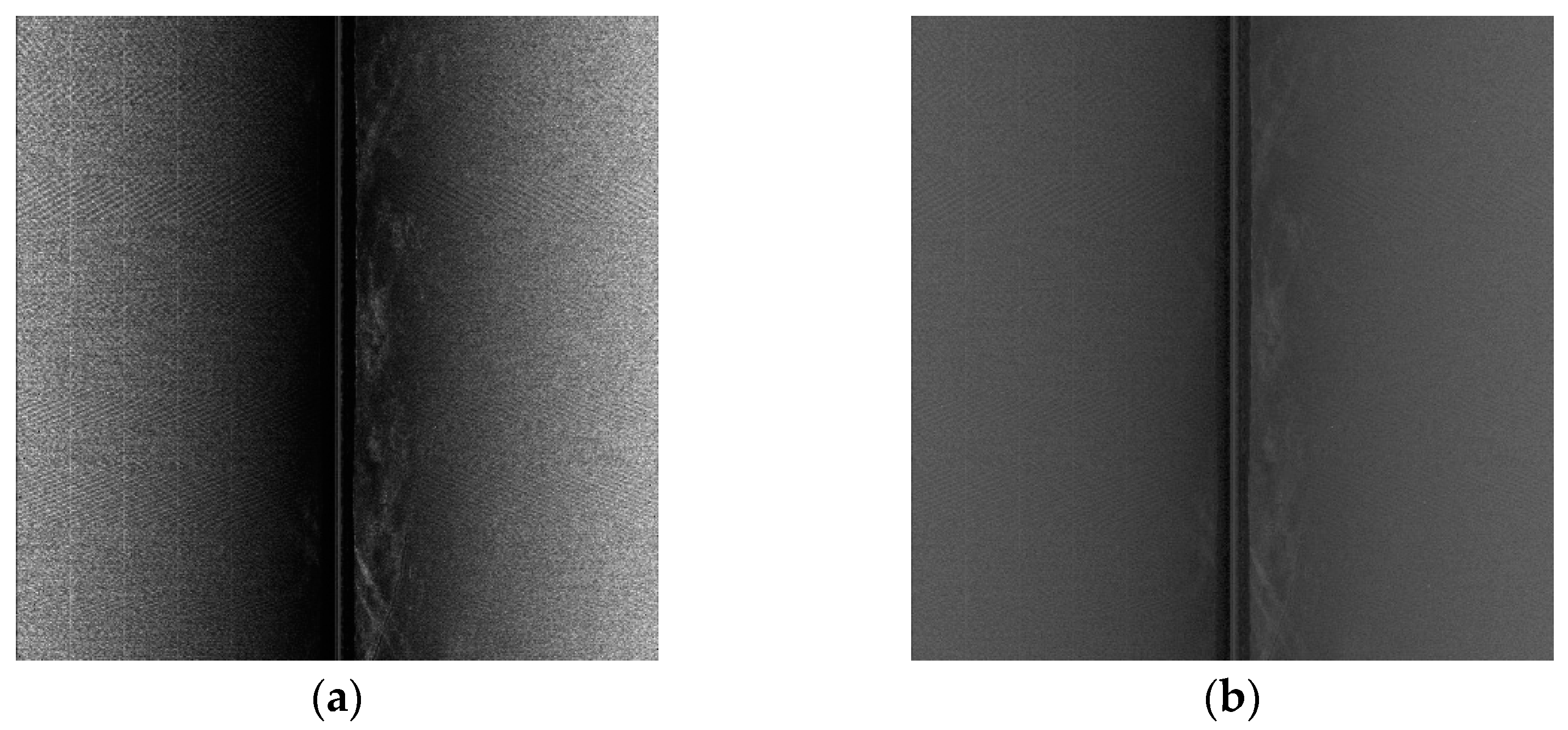
2.2.3. Real-Time Radiometric Distortion Correction

The key to correcting radiometric distortion in SSS images involves determining the baseline and adjusting for the gain variation of the SSS during surveying. For this reason, we propose a radiometric distortion correction method based on prior knowledge.

The change in SSS echo intensity is related to the height of the AUV from the seabed. According to the energy equation, when the initial energy level is fixed, as the height of the AUV above the seabed increases, the echo intensity of the image decreases due to the increase in transmission loss. Therefore, based on historical SSS images, the average echo intensity BS₀ can be calculated at different heights, and data pairs of AUV height and BS₀ can be formed.

$$\{({BS}_{10}, D_1), ({BS}_{20}, D_2), \dots , ({BS}_{n0}, D_n)\}$$

(14)

For an AUV height D_i, the corresponding echo intensity average BS_i0 is obtained by calculating the average echo intensity of two areas in the corresponding image.

As shown in Figure 5, the average echo intensity of the left side image area, −32°~−28°, and the right side image area, 28°~32°, is used as the echo intensity baseline for the corresponding depth D_i. Supposing there are m echo intensities at this height for the AUV in this area, then:

$$B{S}_0^i=\frac{1}{m}{\displaystyle \sum _{j=1}^{m}B{S}_j}$$

(15)

Based on the above sequence, a relationship model is established between the baseline and the AUV height:

$$B{S}_0^{}(D)=a_0+a_{0}D+a_0{D}_{}^2$$

(16)

Using the above model, the AUV height obtained from the previous seafloor line tracking can be substituted into the above formula to obtain the baseline for the SSS at different AUV heights. After obtaining the baseline for radiometric distortion correction, the correction curve is determined. Still taking the echo intensity data of the current ping and the previous 10 pings, averaging the same beam, a correction sequence corresponding to the angle θ is obtained, as follows:

$$\{(B{S}^q{{}^1}_0, q_1), (B{S}^q{{}^2}_0, q_2), \dots , (B{S}^q{{}^k}_0, q_k)\}$$

(17)

Therefore, for a ping sequence, there exists a sequence

$$\{(B{S}^q{}^1, q_1), (B{S}^q{}^2, q_2), \dots , (B{S}^q{}^k, q_k)\}$$

(18)

Combined with the above baseline and correction sequence, the echo intensity correction corresponding to the angle θ in this ping is as follows:

$$\left(B{S}^{\theta }\right)=B{S}_0(D)+(B{S}^{\theta }-B{S}_0^{\theta })$$

(19)

All echo intensity data in the ping are processed in a similar manner to complete the real-time correction of this ping’s radiometric distortion, as shown in Figure 6.

Simultaneously, it can be seen in Figure 7 that after combined radiometric distortion correction, the grayscale changes uniformly within the strip on the left and right sides, the image quality improves, and the visual image quality improves significantly.

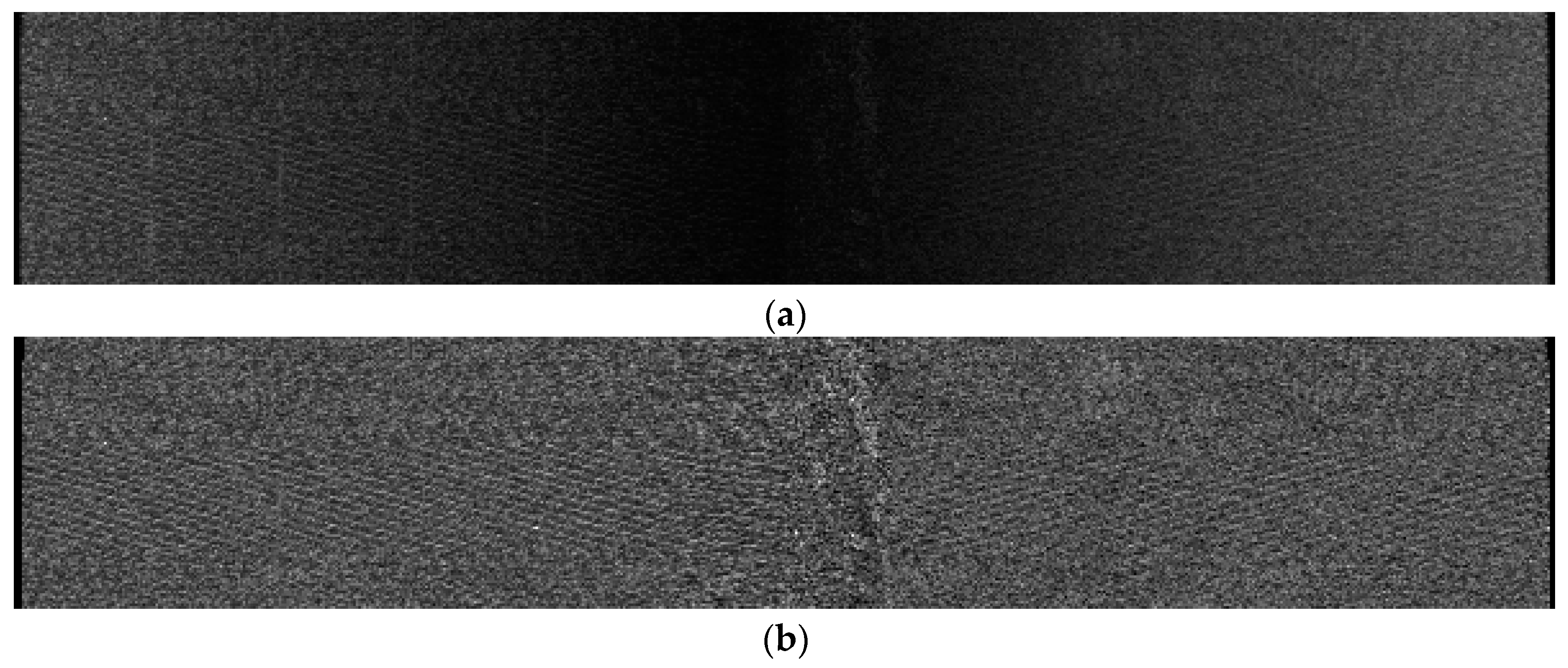
2.2.4. Real-Time Noise Reduction

The presence of noise in SSS measurement data is inevitable. Noise reduces the quality of the data, resulting in many irregular spots in the image, severely affecting the quality of the underwater terrain image. The purpose of SSS denoising is to eliminate or weaken the impact of noise on high-quality mapping while retaining as many of the image features as possible.

The key to denoising SSS images is to suppress noise while preserving valid information. Real-time denoising image processing needs to consider both denoising effects and efficiency. The Alternating Direction Method of Multipliers (ADMM) can quickly denoise SSS images while retaining image details, and can still achieve better visual effects for images with large amounts of texture.

ADMM is a computational framework for solving convex optimization problems. It has the advantages of a fast processing speed and good convergence performance. ADMM decomposes large global problems into smaller, easier-to-solve local sub-problems when dealing with large-scale distributed optimization problems, and then coordinates the solutions of local sub-problems to obtain the solution to the large global problem. The general form of ADMM is as follows:

$$\underset{x,z}{\min } f(x)+g(z)$$

(20)

$$s.t.Ax+Bz=C$$

(21)

where $x\in R^n$ and $z\in R^m$ are the optimization variables, $A\in R^{p\times n}$ and $B\in R^{p\times m}$ are the equality constraints, and f, g both are the objective functions are all convex functions.

The core of the ADMM algorithm is the augmented Lagrangian method (ALM) of the original dual algorithm. The Lagrangian method can be used to solve optimization problems with multiple constraint conditions. This method converts an optimization problem with n variables and k constraint conditions into a problem where a set of equations with n + k variables is to be solved. The augmented Lagrangian method adds a penalty term on this basis to speed up the convergence of the algorithm. The augmented Lagrangian form of ADMM is as follows:

$$L(x,z,\lambda )=f(x)+g(z)+{\lambda }^T(Ax+Bz-C)+\rho /2\ast \left|\right|Ax+Bz-C|{|}_2^2$$

(22)

Using the dual ascent method, we fix two of the variables and update the third, obtaining the iterative optimization process as follows:

$$\mathrm{Step}1: x^{k+1}=\arg {\min }_{x}L(x,z^k,{\lambda }^k)$$

(23)

$$\mathrm{Step}2: z^{k+1}=\arg {\min }_{z}L(x^{k+1},z,{\lambda }^k)$$

(24)

$$\mathrm{Step}3: {\lambda }^{k+1}={\lambda }^k+\rho (Ax+Bz-C)$$

(25)

The above three steps are performed repeatedly until convergence.

3. Experiments and Analysis

3.1. Data Preparation

To verify the correctness of the real-time processing method for AUV-equipped SSS for swath data proposed above, an AUV equipped with an SSS measurement device was used in a water area of 3000 m × 660 m in Bohai Bay, with a water depth change of 845 m and a lot of suspended matter. The SSS system adopts Analog and Digital (DSSS), which contains two frequencies: 100 kHz and 410 kHz. The single side-scan amplitude of the SSS was set to 150 m, the common coverage rate between swaths was 60%, and five measurement lines were laid out in the measurement area, allowing full measurement coverage of the entire water area. During the measurement process, the AUV speed was controlled to vary between 0.5 and 3.5 knots, the water depth varied between approximately 5 m and 9 m with the speed change, and the measurement positions were distributed as shown in Figure 8. The data processing module used was an NVIDIA Jetson Orin NX, the hardware environment was the Windows operating system, and the CPU was a 1024-core NVIDIA Ampere architecture GPU with 32 Tensor Cores. The CPU was a six-core Arm Cortex-A78AE v8.2 64-bit CPU.

3.2. Analysis and Evaluation of Key Technologies in Strip Data Processing

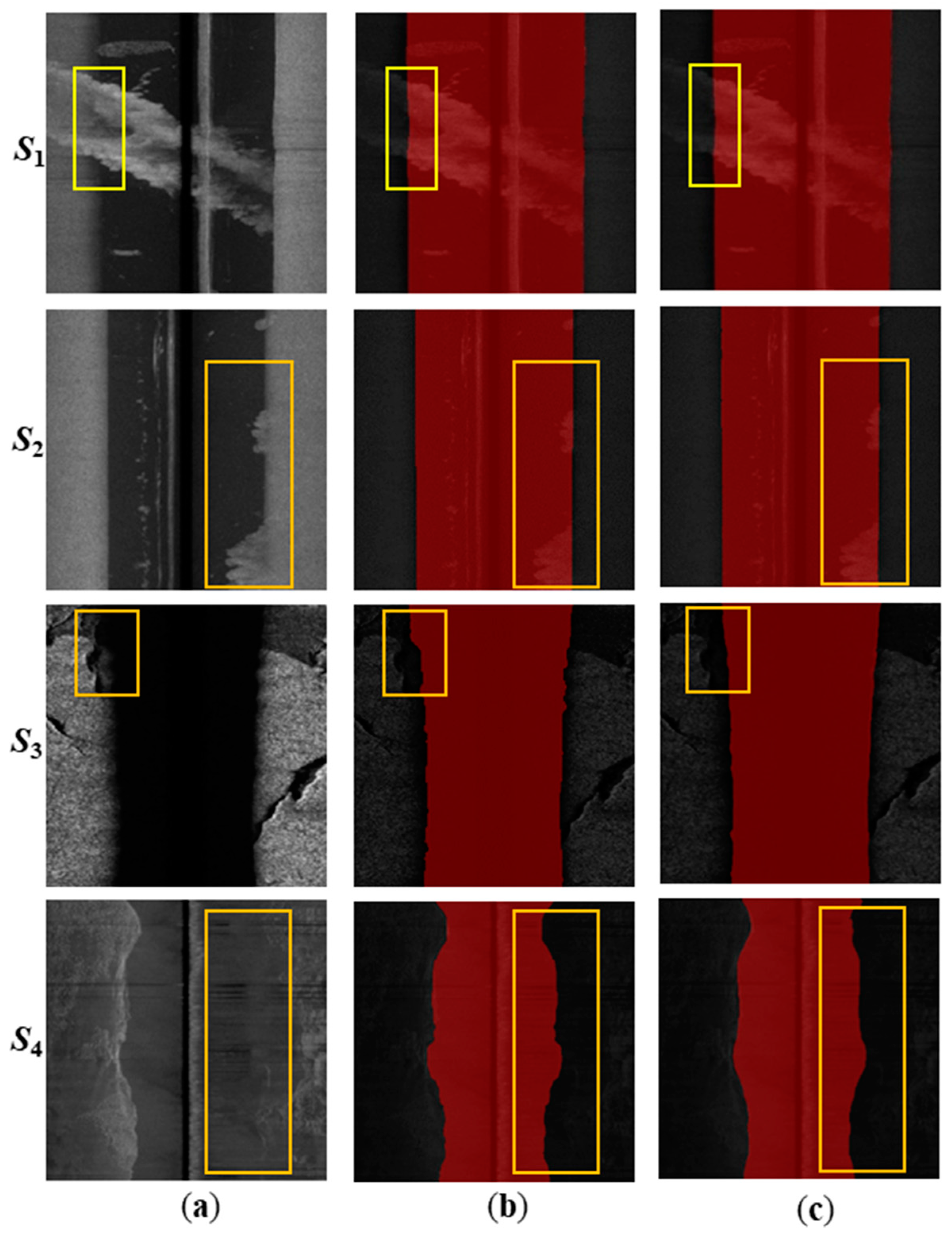
3.2.1. Automatic Seabed Line Tracking

To verify the correctness of the seabed line tracking algorithm, we decoded and performed quality control on each strip’s original observation file in the eXtended Triton Format (XTF) of the SSS. XTF is a prevalent format used for underwater sonar data storage, and provides a standardized method for storing and exchanging various types of sonar data. After obtaining the original waterfall images of each strip, automatic seabed line tracking was carried out in consideration of the distribution characteristics of the waterfall images.

First, we built a semantic segmentation model training dataset. The original SSS waterfall image is quite large, making it difficult to use directly as model input. It can be truncated in the direction of the vertical track line, and there can be some overlap between adjacent truncations. A total of 818 images were obtained, of which 759 were used as the training set and 159 as the test set. The model was trained over 200 batches. The tracking results of the model on the waterfall images with different interferences are shown in Figure 9.

In the S₁ sample, there are a large amount of suspended particles in the water column area. Despite the bottom echo in some pings in the port side image being drowned out by the strong echo produced by the suspended particles, the model can still achieve good results due to the neural network’s strong context acquisition ability. In the S₂ sample, the seabed line in the port side image is very clear, and both models are able to correctly segment the port side image. Some of the seabed lines in the starboard image are covered by strong echoes in the continuous ping, but the model can still correctly segment the starboard side, because it can simultaneously integrate the echo information from the port and starboard sides. The bottom material is strongly absorbing in the S₃ sample, making it difficult to distinguish the boundary between the seabed area and the water column area in some pings in the port-side image. The model still achieves good segmentation results. In the S₄ sample, there is serious noise interference, which results in a low contrast between the water column area and the seabed area in the image. The model is able to estimate the range of the water column area in the starboard image based on the distribution of the water column area in the port side image, thereby obtaining a more accurate segmentation result.

The accuracy of seabed tracking directly affects the correction effect of image radiometric distortion and the measurement accuracy of the seabed target shape. Therefore, it is necessary to evaluate the accuracy of the obtained seabed lines. Accuracy evaluation can be checked on the basis of the completeness of the target contour.

When the SSS images possess a fixed scan amplitude, the width of the original strip waterfall image will be equal, and the width of the water column area image will vary with the distance between the towfish and the seabed. When the towfish depth is constant, the width of the water column area will be high in deep water areas and low in shallow water areas. The water column area is caused by the propagation time of sound waves in the water body and must be eliminated by using the towfish height or water column area width obtained from seabed tracking, with the assistance of slant range correction. If there is a target on the seabed directly below the towfish, and the seabed tracking is correct, theoretically, the target images on the left and right sides will be compressed to the same extent after slant range correction, and the target image contour formed will be continuous, as shown in Figure 10c; otherwise, it will be discontinuous, as shown in Figure 10b. Therefore, the continuity of the target contour after slant range correction can be used to evaluate the correctness of seabed tracking.

One of the stripe images in the Bohai Bay area was tracked for the seabed line, using both the traditional threshold method and the seabed line automatic tracking method proposed in this paper, while considering the distribution characteristics of waterfall images. The tracked seabed lines are shown in Figure 11. As can be seen from the two boxed areas in Figure 11a, the traditional threshold method results in abnormal seabed line tracking when there are suspended objects underwater and the seabed possesses weak absorption, which is mainly due to the fact that the threshold method detects the seabed based on echo intensity or grayscale changes. The method in this paper integrates the semantic information of the seabed in the previous and subsequent pings, considers symmetry, and is effectively able to track the correct seabed on the basis of previous and subsequent pings, combining connectivity and symmetry, solving the problem of abnormal tracking at the location of suspended objects and weakly absorbing bottom material. Therefore, the correct seabed line tracking is presented in the boxed area in Figure 11a, and requires only 0.4 s, which means that not only is the automatic tracking of the seabed line better realized compared with the traditional method, but good real-time performance, robustness and correctness is also achieved.

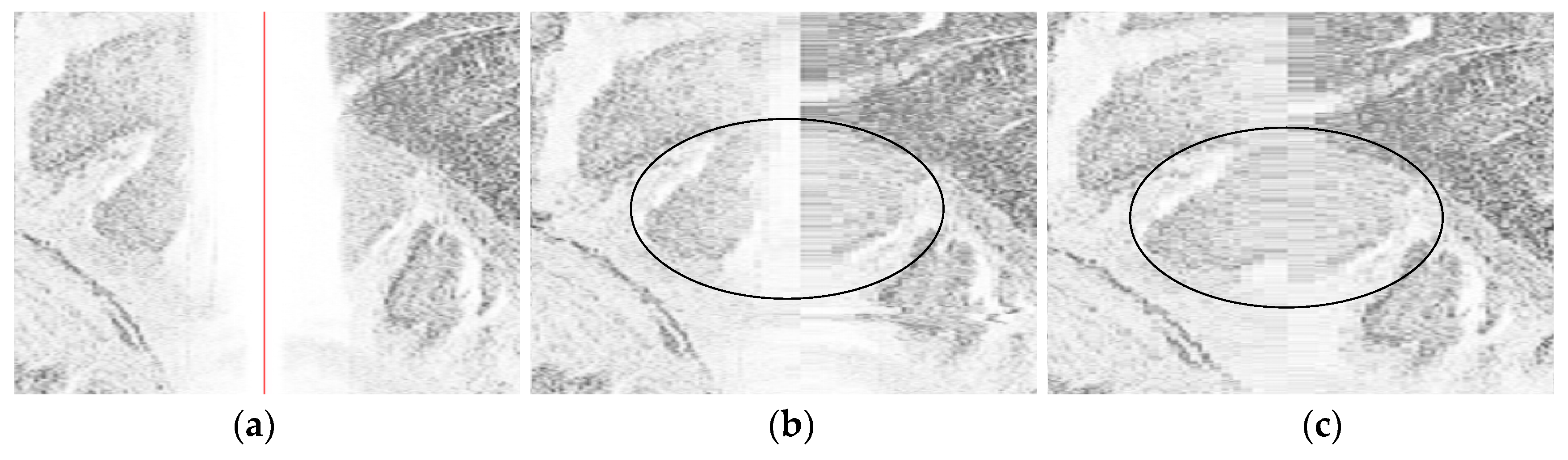
3.2.2. Radiometric Distortion Correction

In order to verify the effectiveness of the radiometric distortion correction proposed in this paper, the waterfall image after seabed line tracking in the Bohai Bay area was selected for radiometric distortion correction. Figure 12a is the original waterfall image, showing that:

(1) There is an area in the central of the strip with a high amount of light, mainly due to the shorter sound wave propagation distance in the central area and the lower amount of energy loss, resulting in stronger echo intensity. This is manifested on the image as an area with a high amount of light, which does not correctly reflect the distribution of seabed material.

(2) In the transverse direction (orthogonal to the navigation track) of the strip image, with increasing sound wave propagation distance, the echo energy loss at the edge becomes greater, and the echo intensity becomes weaker, which is manifested in the image as darker color.

The random carry empirical compensation model can correct the above problems, but this correction is often not thorough due to the difference between the parameters of the empirical model and the actual water area, and the problem of uneven grayscale in the transverse direction still exists. The radiometric distortion correction method proposed in this paper is able to effectively eliminate the incomplete compensation problem caused by propagation loss of transverse echo intensity (grayscale). Figure 13b shows the results after correction using the method proposed in this paper. It can be seen that after slant distance correction and radiometric distortion correction, the grayscale of the image becomes more uniform in the transverse direction, correctly reflecting the distribution of the seabed material and the changes in geomorphological features. In addition, the time required to correct the radiation distortion is only 1 s, which meets the requirements of real-time processing.

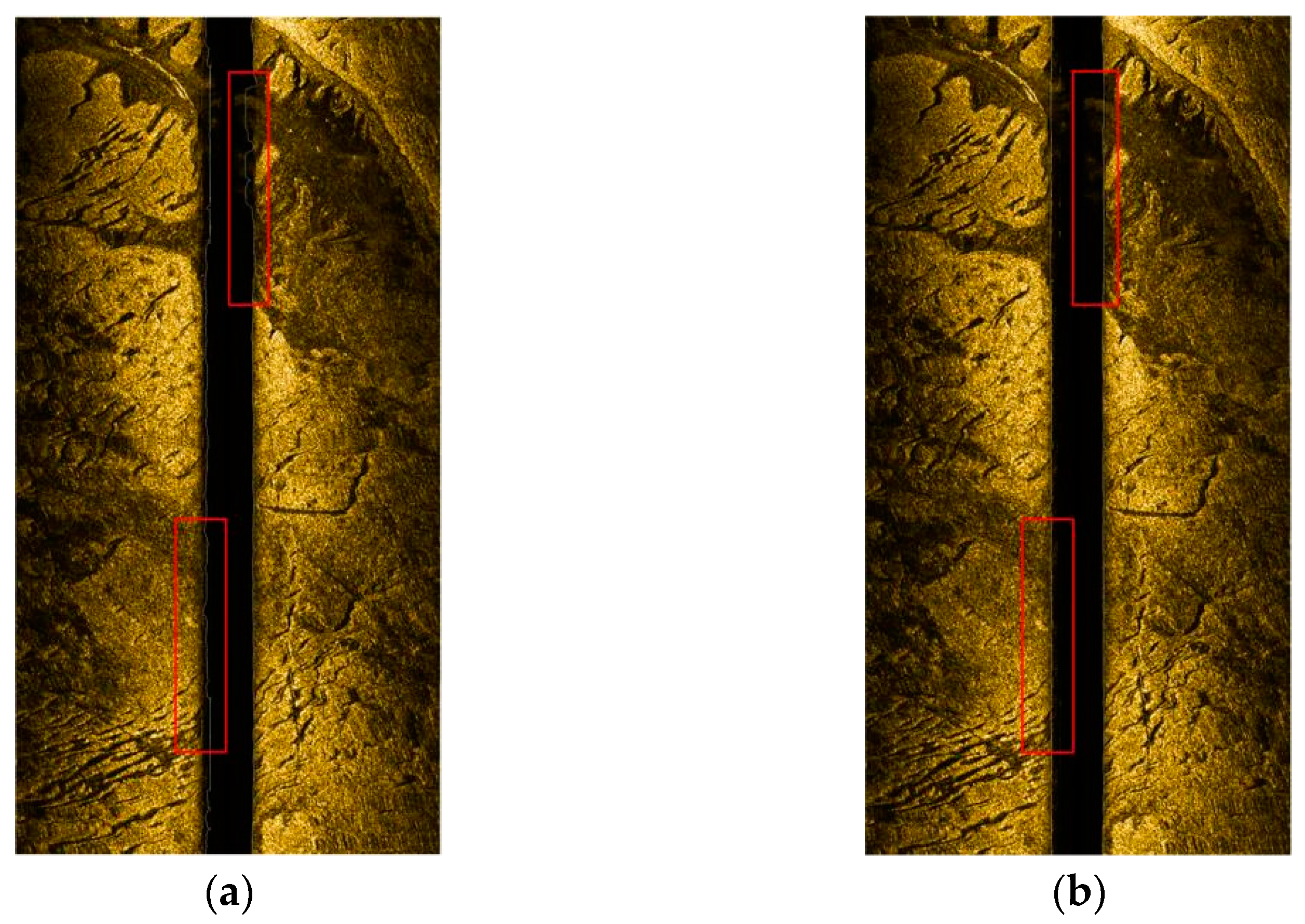
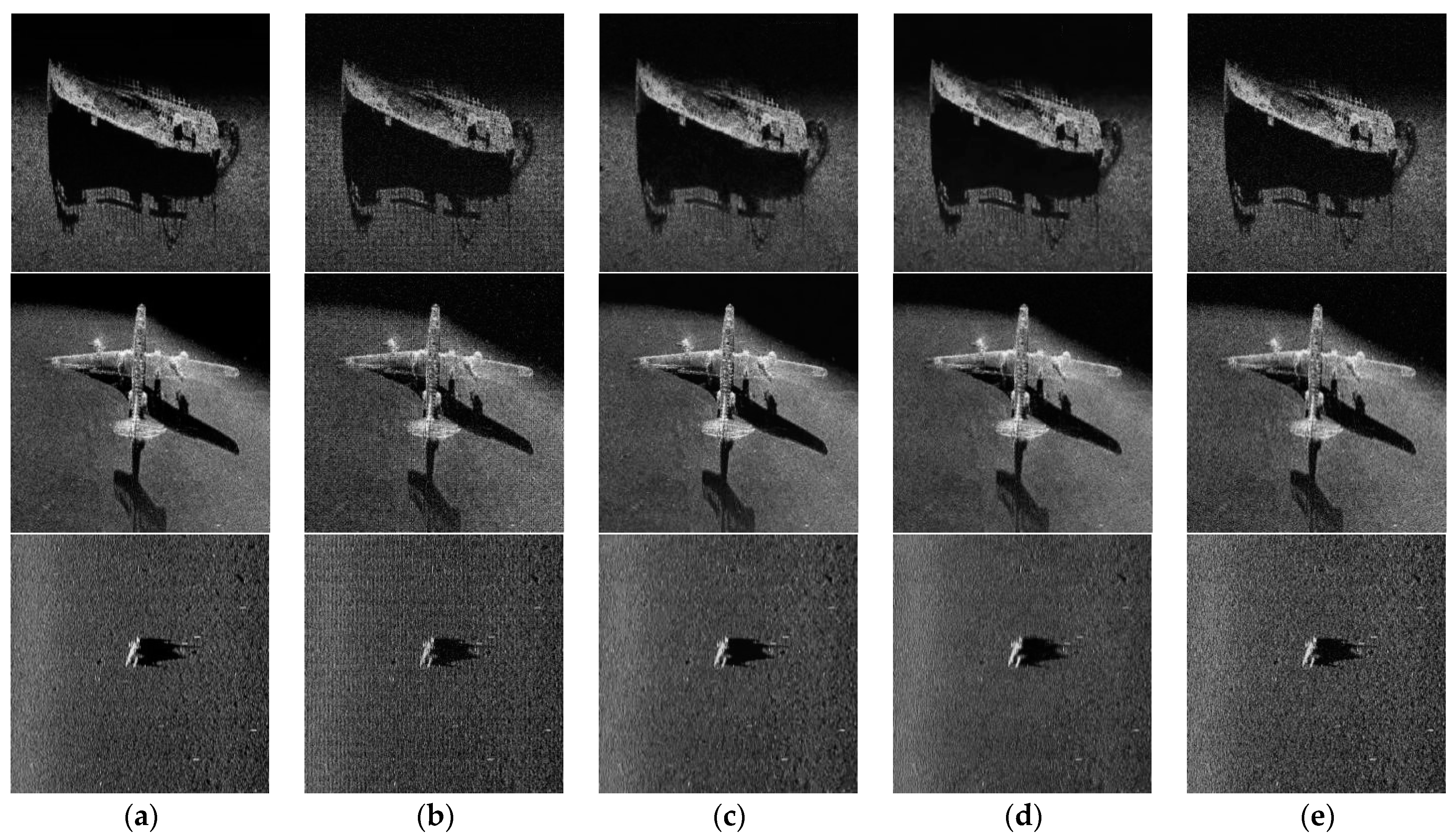
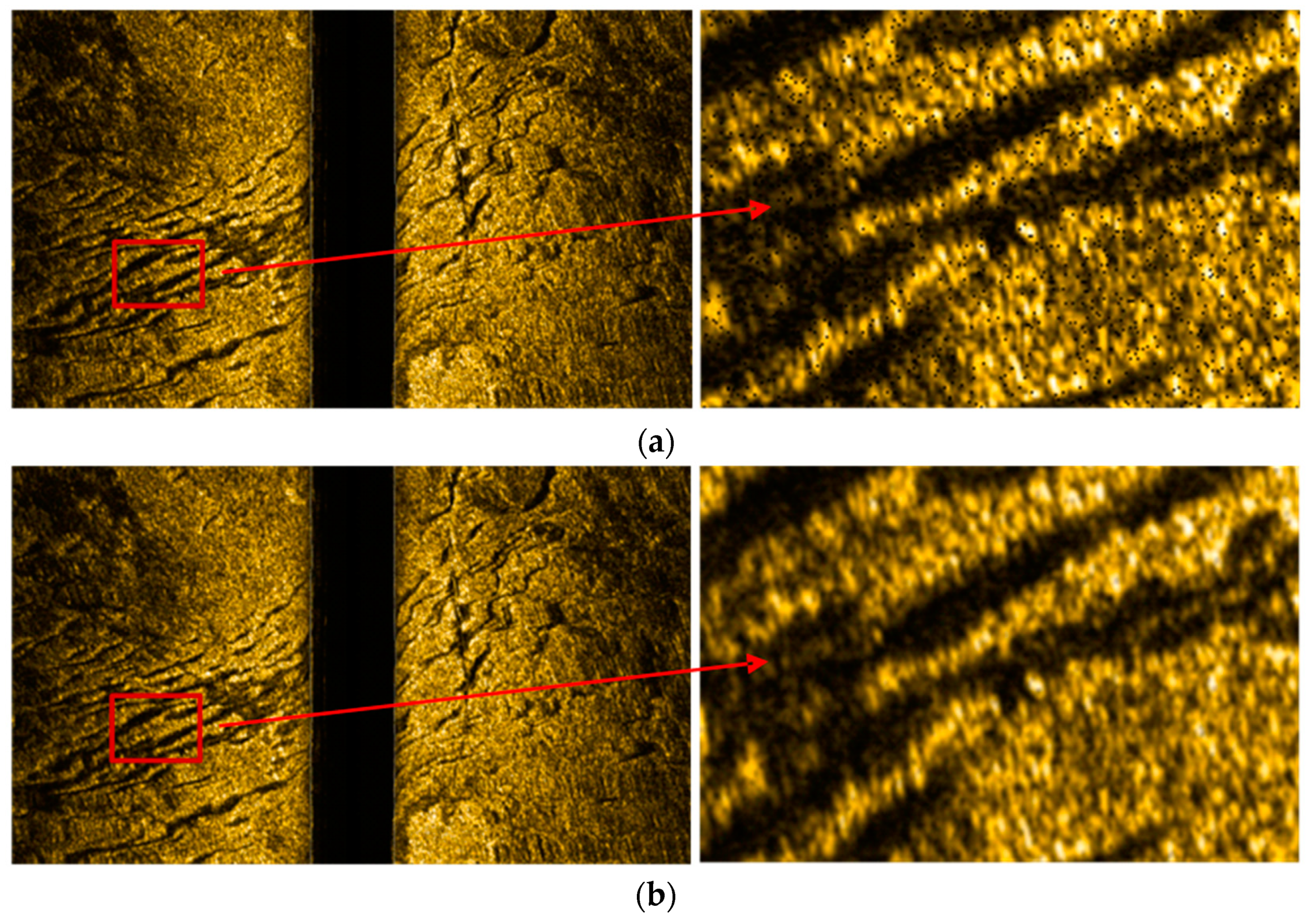
3.2.3. Real-Time Noise Reduction

The results of the SSS image noise reduction experiment are evaluated from two main perspectives: qualitative and quantitative.

Qualitative evaluations are mainly performed based on subjective vision, and quantitative evaluations mainly use the peak signal-to-noise ratio (PSNR) of the image to evaluate the distortion performance of image noise reduction. The PSNR represents the logarithmic value of the mean square error between the original image and the processed image relative to ${(2^n-1)}^2$; the formula is as follows:

$$\{\begin{array}{l}MSE=\frac{1}{H\cdot W}{\displaystyle \sum _{i=1}^H{\displaystyle \sum _{j=1}^W{(X(i,j)-Y(i,j))}^2}}\\ PSNR=10{\log }_{10}(\frac{{(2^n-1)}^2}{MSE})\end{array}$$

(26)

In the formula, MSE represents the mean square error between the denoised image X and the original image Y. H and W are the heights and widths of the two images, respectively; n is the number of bits per pixel, the unit of PSNR is dB, and the higher the value, the smaller the image distortion.

This experiment used three different images for testing, namely, a shipwreck image, an airplane wreckage image, and a frogman image. Of these, the shipwreck image is a local image obtained via SSS imaging, containing less noise, but with rich texture detail. This is used to test the effect of the algorithm on image texture detail during the noise reduction process. the airplane wreckage image is a local image obtained via SSS imaging; the texture is unclear, but the contour is obvious. It is used to test the impact on weak targets during the noise reduction process. In the frogman image, due to the water quality and the smaller size of the frogman, the resolution of the image is lower. It is used to test the effect of the noise reduction algorithm on low-resolution images. In addition, in order to better analyze the effect of image denoising from a qualitative perspective, grayscale images are used for display to avoid the influence of pseudocolor on image judgment, as well as to better compare the differences in denoising performance between algorithms.

Based on an analysis of the above experimental results in

Table 1. Comparison of peak signal-to-noise ratios (PSNRs) after image denoising.

Experimental Image	Methods	PSNR
Aircraft wreckage	ADMM	25.4163
	flexISP	23.4488
	DeepJoint	21.3642
Shipwreck	ADMM	26.7860
	flexISP	24.2550
	DeepJoint	22.1005
Frogman	ADMM	21.3677
	flexISP	21.3410
	DeepJoint	19.3762

, of these four methods, DeepJoint exhibits the poorest denoising capability, while the ADMM method excels, having the best denoising performance. When considering the signal-to-noise ratio of the image, the ADMM method exhibits the highest similarity after post-processing, with the results being more aligned with human perception from a visual standpoint. The shipwreck image predominantly contains Gaussian random noise. While DeepJoint suppresses this noise to a certain extent, it also compromises the detailed texture of the shipwreck, leading to a blurred image. The signal-to-noise ratio of the processed image is noticeably lower than that of the other methods, indicating that it possesses the most significant image distortion. The ADMM method demonstrates superior noise removal with minimal distortion, showing improvements of 4.69 and 6.79 compared to flexISP and DeepJoint, respectively. The airplane wreckage image, conversely, has comparatively limited texture information and is of lower resolution. Following denoising with DeepJoint and flexISP, the image appears blurrier. However, the ADMM method manages to remove noise while preserving the delineation between ground objects and the seafloor, with improvements of 1.97 and 4.05, respectively, being observed over flexISP and DeepJoint. The frogman image is inherently blurred, and under low resolution, the blurring of the image edges by DeepJoint and flexISP becomes more pronounced. The denoising by ADMM is more distinct, but to a certain degree, the visual distortion is also more apparent, showing improvements of 0.027 and 1.99, respectively, compared to flexISP and DeepJoint. In summary, ADMM can eliminate or mitigate the impact of noise while ensuring minimal distortion of side-scan sonar images with varying resolutions, degrees of clarity, and sizes. Most notably, its noise reduction aligns most closely with human visual perception.

The real-time noise reduction method proposed in this paper was used to perform real-time noise reduction corrections on the waterfall map; a comparison of the results before and after is shown in Figure 14.

From the comparative analysis of the effect of noise reduction in the above images, it can be seen that the method proposed in this paper can effectively eliminate the noise in the SSS waterfall image, while retaining the texture information and background information of the image itself; the noise reduction effect is good, and the time required is only 0.6 s.

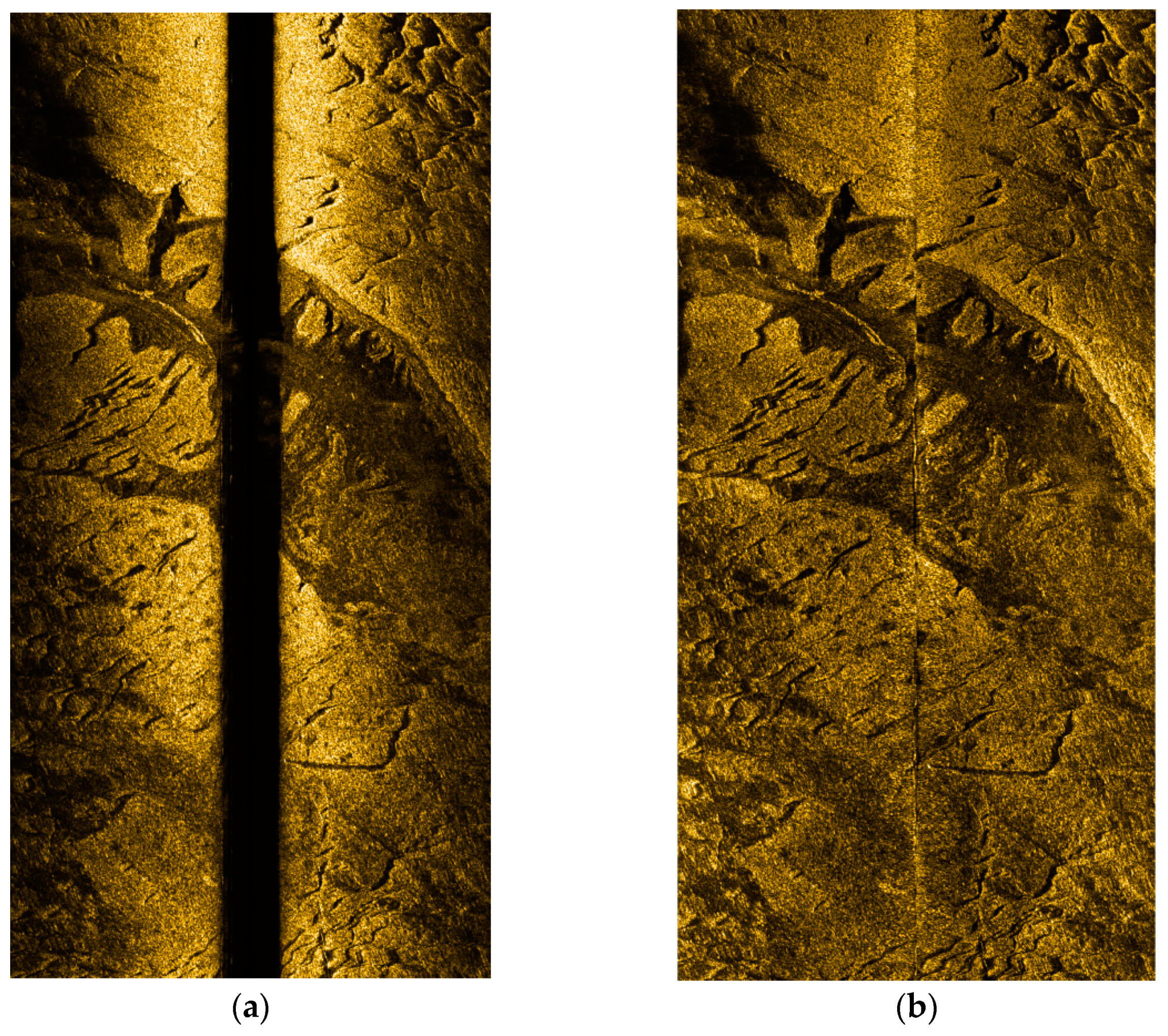
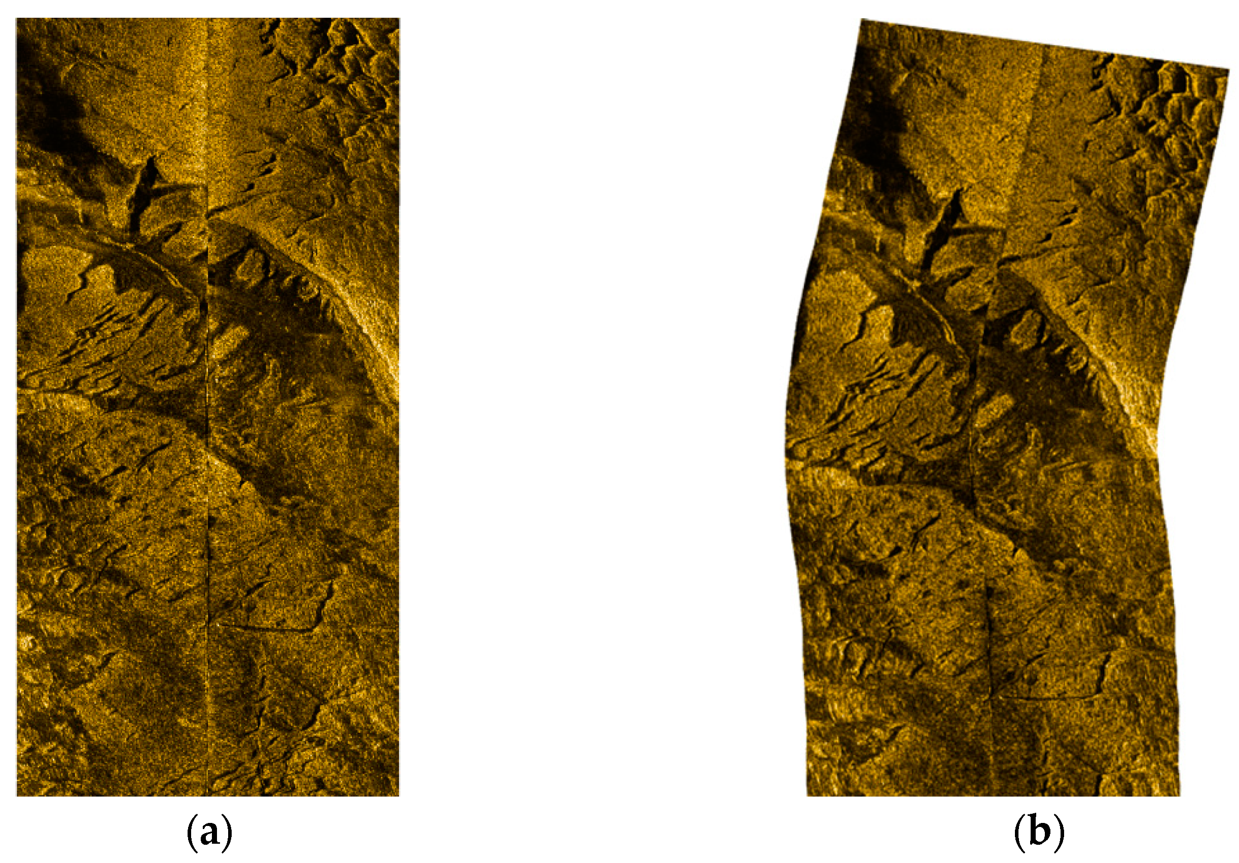
3.2.4. Geographic Coding and Swath Image Stitching

After the real-time bottom line tracking, radiation distortion correction, and noise reduction processing of the original data, a high-quality single-swath along-track image was obtained. In order to further obtain a high-quality swath image with geographic coordinates and realize large-area image stitching based on geographic coding, the waterfall map is corrected for slant distance on the basis of the seabed line extraction results. After the waterfall image has been corrected for slant distance, theoretically, the pixel in the center of each row corresponds to the position directly below the AUV. The geographic coordinates of the pixel in the middle of each row can be determined on the basis of the AUV’s position. Each row of pixels is perpendicular to the current heading of the AUV, and the width from each pixel to the center is all plane distance. Based on the above relationship, the position of each echo in terms of geographic coordinates can be calculated, and the geographic coding of a single swath image can be achieved, as shown in Figure 15.

After real-time processing of the original data of the SSS, a high-quality SSS swath image with geographic coordinates was finally obtained. In order to obtain a large-area seafloor sonar image, it is necessary to mosaic multiple swath images after geographic coding to form a large-area seafloor topographic image. The five swath images measured in this area were processed as described above to obtain geographic coded images, and then the stitching of all swath images was performed in real time, and the resulting seafloor topographic image of the area is shown in Figure 16. The cumulative amount of time required for a single strip was about 3 s, and the total time was about 15 s.

4. Conclusions and Recommendation

In this paper, research was performed on a real-time processing and high-quality mapping method for SSS swath data obtained from an AUV, providing a process for real-time data processing, and solving the four key difficulties related to the real-time processing of SSS data, namely, real-time quality control of the original data, real-time automatic tracking of seabed lines, real-time correction of radiation distortion, and real-time image denoising. Real-time processing and acquisition of SSS swath images from an AUV was achieved, laying the foundation for the smooth implementation of highly time-sensitive tasks such as underwater real-time target detection. The primary contributions of this paper can be summarized as follows:

• Overview of post-processing procedures and methods for side-scan sonar data: A detailed analysis was conducted on the main issues faced by current methods when performing real-time processing.
• Real-time quality control of original observational data: A new control procedure was proposed, including the fusion of INS and DVL navigation data using Kalman filtering, bi-directional filtering methods for echo intensity, and a data filtering method using sliding average or comparison with seabed line tracking for altimeter and pressure gauge data.
• Automatic seabed line tracking: Based on the characteristics of waterfall images, a method based on the Unet network was designed. For real-time processing of single-swath data in the Bohai Bay, this method took only 0.4 s, achieving a high level of accuracy that was consistent with the post-processing results.
• Real-time correction of radiometric distortion: A method was introduced for automatically determining the baseline based on historical echo data. For real-time single-swath data in the Bohai Bay, this method was able to achieve angle-related radiometric distortion correction within 1 s.
• Real-time noise elimination: A method based on the Alternating Direction Multiplier Method (ADMM) was introduced for real-time noise elimination. For real-time processing of single-swath data in the Bohai Bay, this method took only 0.6 s, significantly improving the signal-to-noise ratio of swath images compared to traditional methods.

Overall, in actual experiments performed in the Bohai Bay, the processing time for real-time single-swath data was approximately 3 s, and the total processing time for five survey lines was also around 3 s, largely meeting the demands for real-time processing.

However, having achieved our current results in real-time processing, areas can be recognized that still need further refinement and enhancement:

• Further Optimization of Real-time Processing: Although we achieved real-time data processing, there is still room for improvement in processing efficiency and immediacy. Our method might face challenges especially in scenarios with large data volumes and complex conditions. Future work should further optimize our algorithm for such scenarios.
• Generalizability and Robustness of the Algorithm: While our real-time processing method performs excellently under certain specific scenarios, its general applicability and robustness remain to be addressed. Future research should focus on ensuring consistent and efficient performance across various scenes and environmental conditions.
• Integration with Other Advanced Technologies: Considering the advancements in modern deep learning and AI technologies, integrating our method with these cutting-edge technologies should be explored to further improve the accuracy and efficiency of data processing.
• Holistic System-Level Considerations: In real-time processing, beyond the algorithm itself, there is a need to consider the synergistic operation of the entire system, including sensor selection, data transmission, and storage, all of which can influence the effectiveness of real-time processing.

To better serve practical marine research and resource exploration applications, we recommend that future studies consider the aforementioned directions in greater depth, aiming to achieve more efficient, accurate, and robust real-time processing methods.

References

1. Arshad, M.R. Recent advancement in sensor technology for underwater applications. Indian J. Mar. Sci. 2009, 38, 267–273. [Google Scholar]
2. Anderson, J.T.; Van Holliday, D.; Kloser, R.; Reid, D.G.; Simard, Y. Acoustic seabed classification: Current practice and future directions. ICES J. Mar. Sci. 2008, 65, 1004–1011. [Google Scholar] [CrossRef]
3. Coiras, E.; Petillot, Y.; Lane, D.M. An expectation-maximization framework for the estimation of bathymetry from side-scan sonar images. In Proceedings of the IEEE Europe OCEANS Conference, Brest, France, 20–23 June 2005; pp. 261–264. [Google Scholar]
4. Johnson, S.G.; Deaett, M.A. The application of automated recognition techniques to side-scan sonar imagery. IEEE J. Ocean. Eng. 1994, 19, 138–144. [Google Scholar] [CrossRef]
5. Petillot, Y.R.; Reed, S.R.; Bell, J.M. Real time AUV pipeline detection and tracking using side scan sonar and multi-beam echo-sounder. In Proceedings of the OCEANS ‘02 MTS/IEEE, Biloxi, MI, USA, 29–31 October 2002; Volume 1, pp. 217–222. [Google Scholar]
6. Sahoo, A.; Dwivedy, S.K.; Robi, P. Advancements in the field of autonomous underwater vehicle. Ocean. Eng. 2019, 181, 145–160. [Google Scholar] [CrossRef]
7. Yu, S.C. Development of real-time acoustic image recognition system using by autonomous marine vehicle. Ocean. Eng. 2008, 35, 90–105. [Google Scholar] [CrossRef]
8. Wu, Y.; Zhao, Y.; Lang, S. Development of Autonomous Underwater Vehicles Technology. Strateg. Study CAE 2020, 22, 26–31. [Google Scholar] [CrossRef]
9. Tang, Y.; Wang, L.; Jin, S.; Zhao, J.; Huang, C.; Yu, Y. AUV-Based Side-Scan Sonar Real-Time Method for Underwater-Target Detection. J. Mar. Sci. Eng. 2023, 11, 690. [Google Scholar] [CrossRef]
10. Coiras, E.; Petillot, Y.; Lane, D.M. Multiresolution 3-D Reconstruction From Side-Scan Sonar Images. IEEE Trans. Image Process. 2007, 16, 382–390. [Google Scholar] [CrossRef]
11. Blondel, P. The Handbook of Sidescan Sonar; Springer Science & Business Media: Berlin/Heidelberg, Germany, 2009; pp. 249–276. [Google Scholar] [CrossRef]
12. Bochkovskiy, A.; Wang, C.Y.; Liao, H.Y. YOLOv4: Optimal Speed and Accuracy of Object Detection. arXiv 2020, arXiv:2004.10934. [Google Scholar]
13. Peng, C.; Fan, S.; Cheng, X.; Cao, Y.; Zeng, G. An Improved Side Scan Sonar Image Processing Framework for Autonomous Underwater Vehicle Navigation. In Proceedings of the 15th International Conference on Underwater Networks & Systems, Guangdong, China, 22–24 November 2021; p. 1. [Google Scholar]
14. Yan, J.; Meng, J.; Zhao, J. Bottom Detection from Backscatter Data of Conventional Side Scan Sonars through 1D-UNet. Remote Sens. 2021, 13, 1024. [Google Scholar] [CrossRef]
15. Zheng, G.; Zhang, H.; Li, Y.; Zhao, J. A Universal Automatic Bottom Tracking Method of Side Scan Sonar Data Based on Semantic Segmentation. Remote. Sens. 2021, 13, 1945. [Google Scholar] [CrossRef]
16. Yu, H.; Li, Z.; Li, D.; Shen, T. Bottom Detection Method of Side-Scan Sonar Image for AUV Missions. Complexity 2020, 2020, 1. [Google Scholar] [CrossRef]
17. Zhao, J.; Yan, J.; Zhang, H.; Meng, J. A New Radiometric Correction Method for Side-Scan Sonar Images in Consideration of Seabed Sediment Variation. Remote. Sens. 2017, 9, 575. [Google Scholar] [CrossRef]
18. Zhao, J.H.; Wang, X.; Zhang, H.M.; Wang, A.X. A Comprehensive Bottom-Tracking Method for Sidescan Sonar Image Influenced by Complicated Measuring Environment. IEEE J. Ocean. Eng. 2017, 42, 619–631. [Google Scholar] [CrossRef]
19. Wang, X.; Wu, Q.H.; Wang, A.X. A Comprehensive Radiometric Distortion Correction Method for Side-scan Sonar. J. Geod. Geodyn. 2018, 38, 1174–1179. [Google Scholar]
20. Wang, A.X.; Church, I.; Gou, J.; Zhao, J.H. Sea bottom line tracking in side-scan sonar image through the combination of points density clustering and chains seeking. J. Mar. Sci. Technol. 2020, 25, 849–865. [Google Scholar] [CrossRef]
21. Wang, A.X. 3D Seabed Terrain Recovery Based on Side-Scan Sonar Images; Wuhan University: Wuhan, China, 2014. [Google Scholar]
22. Buscombe, D. Shallow water benthic imaging and substrate characterization using recreational-grade sidescan-sonar. Environ. Model. Softw. 2017, 89, 1–18. [Google Scholar] [CrossRef]
23. Shih, C.C.; Horng, M.F.; Tseng, Y.R.; Su, C.F.; Chen, C.Y. An Adaptive Bottom Tracking Algorithm for Side-Scan Sonar Seabed Mapping. In Proceedings of the 2019 IEEE Underwater Technology (Ut), Taiwan, China, 16–19 April 2019. [Google Scholar]
24. Zerr, B.; Mailfert, G.; Bertholom, A.; Ayreault, H. Sidescan Sonar Image Processing for AUV Navigation. Eur. Ocean. 2005, 1, 124–130. [Google Scholar]
25. Langer, D.; Hebert, M. Building qualitative elevation maps from side scan sonar data for autonomous underwater navigation. In Proceedings of the IEEE International Conference on Robotics and Automation, Sacramento, CA, USA, 9–11 April 1991; Volume 3, pp. 2478–2483. [Google Scholar]
26. Chen, G.Y.; Bui, T.D. Image denoising with neighbour dependency and customized wavelet and threshold. Pattern Recognit 2005, 38, 115–124. [Google Scholar] [CrossRef]
27. Acosta, G.G.; Villar, S.A. Accumulated CA-CFAR process in 2-D for online object detection from sidescan sonar data. IEEE J. Ocean. Eng. 2015, 40, 558–569. [Google Scholar] [CrossRef]
28. Ding, G.; Song, Y.; Guo, J.; Feng, C.; Li, G.; Yan, T.; He, B. Side-scan sonar image segmentation using kernel based extreme learning machine. In Proceedings of the 2017 IEEE Underwater Technology (UT), Busan, Republic of Korea, 21–24 February 2017; pp. 1–5. [Google Scholar] [CrossRef]
29. Long, Z.Y. A sea surface detection and eliminating method of side-scan sonar image. Hydrogr. Surv. Charting 2022, 42, 13–17. [Google Scholar]
30. Huang, X.D. A new image fusion method based on Laplacian pyramid in wavelet field. Electron. Sci. Technol. 2014, 27, 170–173. [Google Scholar]
31. Ye, X.; Li, P.; Deng, Y. A side scan sonar image denoising algorithm based on compound of fuzzy weighted average and Kalman filter. In Proceedings of the 2012 IEEE International Conference on Mechatronics and Automation, Chengdu, China, 5–8 August 2012; pp. 720–724. [Google Scholar]
32. Tin, H.W.; Leu, S.W.; Wang, F.T.; Wen, C.C.; Chang, S.H. Denoising Algorithm Based on Fractal-Wavelet coding and its Application to Side-scan Sonar Image. In Proceedings of the 2013 International Symposium on Physics and Mechanics of New Materials and Underwater Applications (PHENMA 2013), Kaohsiung, Taiwan, 5–8 June 2013; p. 30. [Google Scholar]
Figure 1. Real-time processing workflow for SSS strip data.
Jmse 11 01769 g001
Figure 2. DVL anomaly handling based on SSS images.
Jmse 11 01769 g002
Figure 3. Factors affecting seafloor line tracking. (a) Wake; (b) suspended matter; (c) water quality change; (d) strong and weak absorption bottom texture; (e) seafloor physical target; (f) interference pulse.
Jmse 11 01769 g003
Figure 4. Unet network structure.
Jmse 11 01769 g004
Figure 5. Determining the SSS echo intensity baseline on the basis of historical images.
Jmse 11 01769 g005
Figure 6. Images before and after radiometric distortion correction. (a) Original waterfall image; (b) image after radiometric distortion correction.
Jmse 11 01769 g006
Figure 7. Images before and after radiometric distortion correction. (a) Slant range correction of the original image; (b) slant range correction after radiometric distortion correction.
Jmse 11 01769 g007
Figure 8. Position of the measurement area.
Jmse 11 01769 g008
Figure 9. Model segmentation results. (a) Sample image; (b) manual annotation; (c) model segmentation results. The effects of different factors affecting seafloor line tracking are marked by yellow boxes.
Jmse 11 01769 g009
Figure 10. Example of the influence of seabed tracking on the edge contour of the image after slant distance correction. (a) Original image; (b) incorrect seabed tracking; (c) correct seabed tracking.
Jmse 11 01769 g010
Figure 11. Seabed line extraction results. (a) Results of the traditional threshold method; (b) results of the method proposed in this paper.
Jmse 11 01769 g011
Figure 12. Comparison of stripe images before and after radiometric distortion correction. (a) Before radiometric distortion correction; (b) after slant distance correction and radiometric distortion correction.
Jmse 11 01769 g012
Figure 13. Effects of different image denoising methods on different images. (a) True value; (b) noise; (c) ADMM; (d) FlexISP; (e) DeepJoint.
Jmse 11 01769 g013
Figure 14. Before and after comparison of the effect of noise reduction. (a) Image before noise reduction; (b) image after noise reduction.
Jmse 11 01769 g014
Figure 15. Images before and after swath geographic coding. (a) Swath planar image; (b) swath geographic coding image.
Jmse 11 01769 g015
Figure 16. Multi-swath image stitching and seabed topography image of the measurement area.
Jmse 11 01769 g016