
Interactions between Surface Waves, Tides, and Storm-Induced Currents over Shelf Waters of the Northwest Atlantic


1
Department of Oceanography, Dalhousie University, Halifax, NS B3H 4R2, Canada
2
Department of Mathematics, Hong Kong University of Science and Technology, Hong Kong, China
3
Department of Oceanography, Hong Kong University of Science and Technology, Hong Kong, China
*
Authors to whom correspondence should be addressed.
J. Mar. Sci. Eng. 2023, 11(3), 555; https://doi.org/10.3390/jmse11030555
Submission received: 9 February 2023
/
Revised: 2 March 2023
/
Accepted: 3 March 2023
/
Published: 6 March 2023
(This article belongs to the Special Issue Numerical Modelling of Atmospheres and Oceans)
Abstract
:A coupled wave–tide–circulation model is used to investigate wave–current interactions (WCIs) over the shelf waters of the Northwest Atlantic (NWA) during Hurricane Earl (2010). WCIs have substantial impacts on hydrodynamics in the upper ocean. The significant wave heights are modulated by WCIs, particularly over regions with strong current gradients, with a reduction up to ~2.1 m (20%) during the storm. Noticeable decreases in surface elevations and tidal currents occur in regions with strong tides such as the Gulf of Maine, mainly due to the wave-enhanced bottom stress. Over regions with weak tidal currents, wave effects on currents are dominated by two competitive processes between wave-induced forces and wave-enhanced mixing. The former strengthens surface currents (up to ~0.55 m/s) and increases the peak storm surge (up to ~0.48 m). The latter is responsible for the reduction in storm-induced surface currents (up to ~0.94 m/s) and anticyclonic modulation of current directions. Vertically, WCIs extend the strong vertical current shear and shift it downward during the storm, which enhances the local mixing and changes the structures of near-inertial oscillations (NIOs). Moreover, tidal currents also change the magnitudes of the NIOs and subtidal currents and affect the intensity of WCIs.
1. Introduction
The most common oceanographic phenomena over coastal and shelf waters (CSWs) include surface gravity waves, ocean currents, tides, and storm surges [1]. Ocean currents vary slowly in space and time with typical spatial scales between O(0.1 km) and O(104 km) and temporal scales between O(1 h) and O(100 years). Tides and storm surges last several hours to days. In comparison, the typical scales of surface waves are in the ranges of 1–1000 m and 1–30 s. Despite their distinctive temporal and spatial scales, these motions can have nonlinear interactions with each other. Wave–current interactions (WCIs) can have first-order impacts in coastal regions [2]. Accurate prediction of these processes remains a great challenge partially due to the complexity of their interactions [2,3]. Quantifying their interactions is thus fundamental and essential for a better understanding of coastal dynamics, which is crucial for many applications in coastal engineering, ship navigation, sediment transport, and biogeochemical processes [4,5,6].
In the presence of ocean currents, WCIs can induce large changes in the wave height, frequency, and direction [3,7,8]. Currents can modify wave frequencies and propagation speeds due to the Doppler effect. Spatially varying ocean currents can induce wavenumber shift and wave refraction [7,8]. Ocean currents also cause the relative wind effect that modifies the relative speeds of winds above the sea surface [9]. In addition, bottom topography is an important factor affecting surface waves over shallow waters [10,11,12,13]. Tides and storm surges change the local water depth and thus affect wave dissipation and propagation over shallow waters [14]. As part of the marine atmospheric boundary layer, surface waves mediate air–sea momentum, heat, and gas fluxes by changing the sea surface roughness [15,16]. Surface waves also generate excessive momentum fluxes on currents through the vortex force [17] or radiation stress [18], which are referred to as wave-induced forces. In the vortex force formulation, the wave-induced forces consist of conservative and nonconservative wave effects. The wave-induced conservative forces include an adjustment of the pressure gradient and the processes due to the Stokes drift (). The Stokes drift interacts with the mean current vorticity forming a Stokes-vortex force () and yields a Stokes–Coriolis force () on the Eulerian momentum balance [19], where is the Coriolis parameter. The wave-induced nonconservative forces are caused by the momentum transfer from wave dissipation processes such as whitecapping and wave breaking [17,19]. In the upper ocean, surface waves facilitate vertical mixing mainly through wave breaking and Langmuir circulation [20,21]. At the ocean bottom, wave activities strengthen the level of turbulence and enhance the bottom stress, which is particularly important over coastal regions [22,23].
Many studies have been made on WCIs over CSWs in recent decades. Xie et al. [24] showed that wave-enhanced bottom stress weakened the near-bottom currents by up to 0.6–0.8 m/s during Hurricane Fran (1996) over the coastal regions of the South Atlantic Bight. The wave-enhanced bottom stress was also found to extensively weaken the bottom currents in the inner Texas–Louisiana shelf [22] and the tidal currents over an energetic tidal area in Western Europe [25]. Conversely, wave-induced forces can generate additional ocean currents through conservative processes related to the Stokes drift and nonconservative processes of wave dissipation [17,19]. Weber and Melsom [26] suggested that wave-induced currents are comparable with the Ekman currents at the surface, which was confirmed by Perrie et al. [27] in the Labrador Shelf. Zou and Xie [28] found that the depth-mean currents over the Georges Bank can be strengthened by ~20% due to wave-induced currents at the storm peak. Wang et al. [29] showed that wave-driven currents can be up to ~1 m/s due to intense wave breaking in Lunenburg Bay during Hurricane Juan (2003). The wave-induced forces were also found to escalate surge elevations in many coastal areas [30,31,32,33]. Kim et al. [30] showed that the wave set-up contributed to the peak storm surge by up to ~40% near the coast of Japan during Typhoon Anita (1970). Liu and Huang [32] showed that the wave set-up had a maximum contribution of 35% to the storm surge near the coast of Taiwan. In addition to the wave set-up due to the wave-induced forces, Bertin et al. [34] showed that wave-enhanced wind stress also contributes to the storm surge for a young sea state and the wave-enhanced bottom stress slightly reduces the storm surge. The wave-enhanced mixing was shown to reduce the sea surface temperature (SST) and deepen the mixed layer, particularly during tropical storms [35,36]. Wang and Sheng [36] showed that surface waves enhanced the storm-induced surface cooling by up to 1.2 °C along the storm track of Hurricane Juan (2003).
Previous studies have also suggested the importance of WCIs over lakes [37] and marginal and enclosed seas [38,39,40]. Although the WCIs were found to have significant impacts in the upper ocean, the dominant mechanisms of WCIs under different ocean conditions can be considerably different and require further investigation. Wave-induced forces, such as wave-breaking acceleration, are usually the primary processes for the WCIs in the surf zone [41,42,43]. Beyond the surf zone, the vertical stratification is relatively strong such that wave-enhanced mixing can play a significant role by mixing up the cool subsurface waters [36,44]. Over energetic tidal areas, the wave-enhanced bottom stress can be crucial in changing tidal currents and can affect subtidal currents [24,45]. Lin et al. [46] recently developed a coupled wave–circulation model for the Northwest Atlantic (NWA) incorporating all the processes of WCIs mentioned above and systematically showed that the processes of WCIs, in combination, produce significant changes in the upper ocean. In the NWA, which has complex dynamics, each process was found to play an important role in some specific areas. Therefore, the exclusion of some important physical processes in many previous studies may lead to different conclusions. Lin et al. [46] examined the WCIs over the deep ocean during two consecutive hurricanes using the coupled model for the NWA. The three-dimensional (3D) WCIs over the CSWs of the NWA under the combined forcing of tidal currents and storm-induced subtidal currents, however, are not well studied. This study, which is a companion study of our previous work [46], provides the first insight analysis on the 3D interactions between surface waves, tides, storm-induced subtidal currents, and near-inertial oscillations (NIOs) over the CSWs of the NWA. Moreover, this study investigates the impacts of these processes and their interactions on the coastal and shelf dynamics and the mechanisms governing the interactions.
The rest of this paper is structured as follows. Section 2 introduces the study region and period. Section 3 presents the methodology used in this study, including the coupled wave–tide–circulation model and observational data. Section 4 shows the model validation. Section 5 investigates the current modulations of surface waves and the impacts of waves on circulation. Section 6 presents the discussion and conclusions.
2. Study Region and Period
The study region is the CSWs and adjacent deep waters of the NWA, covering the regions from Cape Hatteras in the south to the Newfoundland and Labrador Shelves (NLS) in the north (Figure 1a). The topography over the study region is highly variable with a complex array of banks, ridges, and gullies. From south to north, the study region comprises the Middle Atlantic Bight (MAB), Georges Bank, Gulf of Maine (GoM), Scotian Shelf, Gulf of St. Lawrence (GSL), Grand Banks, and NLS. In addition to the constraint by the bottom topography, the general circulation over this region is affected by local winds, tides, river runoff, and large-scale circulation, such as the Gulf Stream and Labrador Current [47]. There are large tidal ranges and strong tidal currents over some CSWs of the NWA, such as the Bay of Fundy, GoM, and northwestern GSL [48]. In the Bay of Fundy, the tidal range is the highest in the world, reaching approximately 16 m because of its geometry [49]. River discharges, especially those from the St. Lawrence River and Hudson River, contribute significantly to the buoyancy flux over the CSWs of the NWA. In the passage of a storm, strong winds generate large surface waves and intense currents in the upper ocean and induce NIOs. With the strong tidal currents, complex circulation patterns, storm-induced currents, and waves, these processes and their interactions jointly affect the hydrodynamics over the study region.
The study period is between 20 August and 20 September 2010, during which Hurricane Earl swept through the continental shelves of the NWA in early September. Earl originated from a tropical wave on 23 August and became a hurricane on 29 August when it approached east of the Lesser Antilles [50]. The storm reached its peak as a Category 4 hurricane when it centered over the southeast of North Carolina on 2 September. Earl then rapidly weakened as it turned northward, remained a Category 1 hurricane to the east of Cape Hatteras early on 3 September, and became a tropical storm over the MAB later on 3 September. The storm restrengthened to a hurricane after passing Georges Bank and made landfall in Nova Scotia on 4 September. Earl became extratropical after passing Prince Edward Island (PEI) and transited through the GSL and NLS on 5 September. Eventually, the storm disappeared in the Labrador Sea (Figure 1).
The choice of Hurricane Earl as a case study in this paper is motivated by the following considerations. Firstly, Earl was one of the major hurricanes that substantially affected the continental shelves of the NWA as it passed by most shelf regions. Secondly, Earl was extensively studied previously in terms of the structure and evolution of the hurricane [51], physical and biological responses of the ocean [52], and air–sea fluxes [53]. However, most of these previous studies did not incorporate the effects of WCIs and focused mainly on the tropical regions rather than the continental shelves ranging from the MAB to NLS.
This study aims to examine the important role of WCIs over the CSWs of the NWA during Hurricane Earl.
3. Methodology
3.1. Coupled Wave–Tide–Circulation Model
The coupled wave–tide–circulation model for the NWA (CWTCM-NWA) is based on the Regional Ocean Modeling System (ROMS, version 3.8) and the Simulating Waves Nearshore model (SWAN, version 41.31), within the Coupled Ocean–Atmosphere–Waves–Sediment Transport (COAWST) modeling platform [54]. The ROMS solves the Reynolds-averaged Navier–Stokes equations on a free surface and terrain-following grid using the Boussinesq and hydrostatic approximations [55]. In the configuration of the CWTCM-NWA, the ROMS incorporates following four mechanisms of wave effects on currents. The wave-induced forces on currents are specified using the vortex force formulation, including the conservative and nonconservative wave effects [17,19]. The wave effect on the sea surface roughness is included using the formula developed recently by Lin and Sheng [16], in which the nondimensional sea surface roughness has different dependencies on the wave age under different sea states. The turbulent closure scheme uses the Generic Length Scale, which includes wave-enhanced mixing by injecting additional turbulence kinetic energy (TKE) [41]. The bottom stress is estimated using the wave–current interaction method proposed by Madsen [56].
The ROMS uses a horizontal resolution of 1/12° and 40 vertical terrain-following layers. The atmospheric forcing is obtained from the fifth generation of atmospheric reanalysis (ERA5) [57]. To well represent the hurricane wind, the wind data from the Hurricane Wind Analysis System (HWIND) during Hurricane Earl are additionally blended into the ERA5 wind using the method suggested by Fan et al. [58]. The tidal forcing uses the Atlantic Ocean database created with the Oregon State University Tidal Inversion Software [59]. The subtidal open boundary conditions and initial conditions are taken from the Global Ocean Reanalysis and Simulation (GLORYS, www.mercator-ocean.eu/en/ocean-science/glorys, accessed on 1 March 2023). The model includes freshwater discharges from 49 rivers based on the data from the United States Geological Survey (USGS, www.usgs.gov, accessed on 1 March 2023) and Environment and Climate Change Canada (ECCC, www.canada.ca/en/environment-climate-change, accessed on 1 March 2023).
The SWAN is a third-generation spectral wave model based on the wave action balance equation [60]:
where is the wave action density defined as , is the wave energy, is the relative wave frequency, is the wave direction, and are the propagation speeds in the frequency and directional spaces, respectively, is the wave group velocity vector, is the wavenumber vector, is the total mean water depth, is a coordinate in the wave direction, and is a coordinate perpendicular to . The ocean current () is the depth-weighted current velocity in the near-surface layer using the formula suggested by Kirby and Chen [61]. The SWAN incorporates physics for wave generation (), wave dissipation (), nonlinear quadruplet () and triad () wave–wave interactions, depth-induced wave breaking (), bottom friction (), and current effects on waves in spatial (Equation (2)) and spectral (Equations (3) and (4)) spaces. The relative wind effect is also considered by subtracting the ocean currents from the winds.
In the configuration of the CWTCM-NWA, the SWAN is driven by the same wind forcing at the same spatial resolution as the ROMS. Ocean currents and surface elevations are specified in the SWAN using results from the ROMS. The open boundaries in the SWAN are forced by wave spectra from a global wave model provided by the French Research Institute for Exploitation of the Sea (IFREMER, iowaga.ifremer.fr/Products). In the SWAN model, the wind input and wave dissipation are computed using the package ST6 [62,63]. The nonlinear quadruplet () and triad () wave–wave interactions are computed using the Discrete Interaction Approximation of Hasselmann et al. [64] and the Lumped Triad Approximation of Eldeberky [65], respectively. The depth-induced wave breaking is computed following Lin and Sheng [66]. The bottom friction is calculated using the eddy viscosity model of Madsen et al. [67]. The wave model has 36 directional bands and 35 frequencies, ranging from 0.04 to 1.0 Hz. In the CWTCM-NWA, the SWAN uses a time step of 300 s, while the ROMS uses a barotropic time step of 6 s and a baroclinic time step of 120 s, to take advantage of using a short time step for the depth-mean dynamic equations and a longer time step for the 3D dynamic equations [55]. The SWAN and ROMS exchange data fields at a time interval of 1200 s. Details on the formulations for WCIs and configurations of the coupled wave–circulation model were presented by Lin et al. [46].
Three basic experiments were conducted for this study, including the wave-only (WO), circulation-only (CO), and fully coupled (FC) model runs (i.e., CWTCM-NWA). To examine the interactions of waves with tidal and subtidal currents, two experiments without the tidal forcing were conducted (i.e., CONT and FCNT in Table 1). Four additional process-oriented experiments were conducted to identify the primary physical processes in the WCIs. In each additional experiment, a specific physical process of wave effects on currents was turned off. Configurations of these nine model runs are summarized in Table 1, together with the abbreviations of each model run.
3.2. Observational Data
The satellite data used in this study included the altimeter wave data obtained from the Australian Ocean Data Network portal, based on the global significant wave heights (SWHs) from 13 altimeters. These altimeter wave data were quality controlled and consistently calibrated against buoys and cross-validated between satellites [68]. All available altimeter wave data tracking through the study region between 20 August and 20 September 2010 were used, with a total of ~390 tracks (Figure 2c).
In situ observations used include wave variables measured at 17 buoy stations, surface elevations measured at 10 tidal gauges, temperature profiles measured by Argo floats, and ocean currents observed at two stations (Figure 1). Argo is an international program that measures global ocean temperature and salinity using drifting profiling floats. The Argo data were found to have high accuracy in comparison with the shipboard measurements [69]. The used Argo data include 160 vertical temperature profiles over the study region during the study period. The salinity data measured by the Argo floats are not presented here as the change in the salinity of the upper layer is not significant over deep waters [46]. The observed currents at two stations (N01 and M01) during the study period were obtained from the University of Maine Ocean Observing System [70]. Station N01 is located on the eastern side of the Northeast Channel connecting the GoM with the open ocean. Station M01 is over the Jordan Basin in the inner GoM (Figure 1). The current velocities were measured at these two stations from near-surface to near-bottom using the downward-facing acoustic Doppler current profilers (ADCP) [70].
4. Model Validation
The performance of the CWTCM-NWA was recently assessed by Lin et al. [46]. The coupled model was shown to improve the accuracy in predicting SWHs, wave periods, wave spectra, surface elevations, SST, and sea surface salinity. The model performance is further assessed in this study using three additional sets of observational data, including the SWHs from altimeters, temperature profiles made by the Argo floats, and current velocities at two ADCP stations (Section 3.2).
4.1. Surface Wave
We first assess the performance of the CWTCM-NWA for wave simulations by linearly interpolating the simulated significant wave heights (SWHs or ) along the altimeter tracks and comparing them with altimeter measurements in scatterplots (Figure 2a,b). The observed SWHs along all the available altimeter tracks during the study period are shown in Figure 2c. Four error metrics defined in Appendix A are used to quantify the model performance, including the root mean square error (RMSE), relative bias (RB), scatter index (SI), and correlation coefficient (R). Values of these error metrics are shown in the four left panels of Figure 2. Most of the simulated SWHs in run WO agree reasonably well with the altimeter data, with a SI of ~19.4% and a correlation coefficient of ~0.943, although the model results in this run generally overestimate the energetic sea states for 5.0 m (Figure 2a). In comparison, run FC has higher accuracy with a smaller SI of 18.8% and a slightly higher correlation coefficient of ~0.945 (Figure 2b). The scatterplot in Figure 2d demonstrates that run WO reproduces reasonably well the small waves with the observed SWHs less than 4.0 m but overestimates the large observed waves at these 17 wave buoys. In comparison, run FC reduces the overestimations of run WO (Figure 2e) and has a smaller SI value of ~23.3% compared with ~24.4% in run WO.
As shown in Figure 2, however, the overall improvement of run FC over run WO is marginal. This is because most of the wave observations were made during relatively gentle sea states when both runs FC and WO have reasonably good skills. The advantage of run FC over run WO becomes clear for the energetic sea states when the WCIs are intense, which is essential in scientific studies and engineering applications. To further illustrate the performance of these two runs, the bin-averaged values of SI for SWHs are calculated using the altimeter data (Figure 2f) and buoy observations (Figure 2g), respectively. The SI represents a normalized mean error, and a smaller value of SI denotes a better agreement with observations [66]. The sea states during the study period were relatively gentle with the majority (90%) of 3.5 m, while large storm waves were mostly observed by the altimeters that have wide spatial coverage. For 3.5 m (90%), run FC (black plus) produces more accurate predictions with lower values of SI compared with run WO (green circle). The improvement by including WCIs is significant for large waves, for which run FC has much smaller model errors than run WO. The reductions indicate the importance of WCIs in temporal and spatial modulations of surface waves. More details will be discussed in Section 5.1.
4.2. Water Temperature
All the available Argo floats during the study period occurred mainly in the deep waters over the study region, with some floats over the NLS (Figure 3a). The observed temperatures of surface waters during this period were relatively warm and ~30 °C along the main path of the Gulf Stream and adjacent deep waters over the southern part of the study region, and relatively cool and less than ~15 °C in the NLS. Since the WCIs significantly affect the upper ocean hydrodynamics [36,46], the observed temperatures in the upper ~250 m are compared with model results in terms of scatterplots. Although the data points are scattered in Figure 3b,c, most of them lie closely above the perfect fitting line (black dashed line) with temperatures of ~5 °C. On average, run CO slightly overestimates the observed temperatures with an RB of ~3.4% and an SI of ~15.8%. In comparison, run FC reduces the overestimation and performs better with an RB of ~3.0% and an SI of ~15.1%.
We next compare the model results with Argo observations for the temperature profiles at six selected locations over the shelf region, continental slope, and deep waters (Figure 3d,i). For the observed profile at site d in the deep waters near the Gulf Stream (Figure 3d), the surface mixed layer had a depth of ~50 m with temperature values of ~28 °C, and the thermocline below extended to a depth of more than several hundred meters. In comparison, for the observed profiles at sites e–h affected by the Labrador Current over the NLS (Figure 3e,h), the observed mixed layer depth (MLD) was shallower within ~20 m. The thermocline at these three sites was within the top ~50 m, where the observed temperature rapidly transited to approximately 5 °C at a depth of ~150 m (Figure 3e,h). These important observed features are generally reproduced in both runs CO and FC, but run FC performs better than run CO in simulating variations of water temperature in the upper ocean. This can be explained by the fact that surface waves deepen the MLD and cool the sea surface waters. In particular, close to the boundary at site i (Figure 3i), run FC well reproduces the observed temperature profile by including the wave-induced inflow of the relatively cold water. The important role of WCIs in ocean currents and water temperature will be further discussed in Section 5.2.
4.3. Ocean Current
To assess the model performance in simulating ocean currents at different frequencies, spectral analyses are conducted for the time series of observed and simulated near-surface and near-bottom currents at stations N01 and M01 during the study period (Figure 4). The power spectra are calculated using the fast Fourier transform and smoothed using a Parzen window with a bandwidth of 0.03 cycles per day (cpd) [8,71]. Analysis of the observed currents shows that the zonal velocity () is dominant at station N01 over the Northeast Channel and the meridional velocity () dominates at station M01 over the Jordan Basin. Figure 4 shows the dominant current components at these two stations. The observed currents at these two stations were dominated by the peak at the semidiurnal (M2) tidal frequency, followed by a notable peak at the near-inertial frequency in the near-surface layer. Meanwhile, the observed currents have large power spectra at subtidal frequencies (<0.5 cpd), which correspond to the subtidal currents driven by Hurricane Earl. The outstanding M2 peaks at these two stations at both depths are reasonably well predicted in both runs CO and FC. Run FC reduces the overestimations of the M2 peaks in run CO, which is mainly attributed to the reduction of tidal energy due to the wave-enhanced bottom stress (see Section 5.2). In comparison with run CO, run FC also performs better in simulating the NIOs, particularly in the near-surface layer. Both model runs (CO and FC), however, underestimate the power spectra at high frequencies (>2.2 cpd), which can be partially attributed to the insufficient resolutions of the model forcing and model grid [72]. Overall, run FC has higher accuracy in predicting the subtidal currents and dominant tidal currents, although it still underestimates the relatively weak currents at high frequencies.
5. Results
5.1. Temporal and Spatial Modulations of Surface Waves
To quantify the current effects on waves, we first examine the simulated SWHs in runs FC and WO and compare them with observations at three typical buoy stations during the study period. The positions of these three buoy stations (44137, 44008, and 44027) are shown in Figure 1. Buoy 44137 is on the right-hand side (RHS) of Earl’s track over the continental rise. At this location, the storm waves predicted in run FC are less energetic with the peak SWH of ~10.2 m compared with ~11.0 m in run WO and agree better with the observed value. The reduction of SWHs on the RHS was also discussed in previous studies [36,46,73,74], partially due to the relative wind effect caused by the storm-induced currents. More details will be discussed in Section 6. Similarly, the peak SWHs become smaller at buoy 44027 (Figure 5c) in the inner GoM by including WCIs. At buoy 44008 (Figure 5b), which is close to the hurricane track, the effect of WCIs is relatively weak for the peak SWHs. At these two buoys (Figure 5b,c), notable oscillations of observed SWHs occurred after the peak winds, which are reproduced in run FC. The oscillations are due to the WCIs associated with the strong NIOs in the wake of Hurricane Earl (also shown in Figure 6). In addition to changes by the storm-induced currents, surface waves are also modulated by tidal currents in the energetic tidal regions, such as near buoys 44008 and 44027. Buoy 44008 is near the Great South Channel between Nantucket Shoals and Georges Bank, while buoy 44027 is in the inner GoM close to the Bay of Fundy. At these two buoys, the intense flood-ebb tidal currents modulate waves at tidal frequencies (also shown in Figure 6). At all the 17 buoy stations during the study period, the SWHs are modulated by currents in a range of −1.0~0.55 m (−16.8%~13.3%) for > 3.0 m, indicating again the importance of WCIs. It should be noted that the absolute (in meter) and relative changes (in percentage) do not necessarily occur at the same time or place.
To identify the temporal modulations of waves by currents at different frequencies, the same spectral analyses are conducted for time series of observed and simulated SWHs at buoys 44008 and 44027 (Figure 6). The power spectra of the depth-weighted meridional currents () at these two stations are also shown in Figure 6a,b, and the coherence spectra between and are shown in Figure 6c,d. It should be noted that the depth-weighted currents in the relatively deep waters are close to the surface currents [61]. At both stations, surface waves have peak energy at low frequencies corresponding to a synoptic time scale of 3–10 days, as surface waves are driven by the storm (red lines in Figure 6a,b). Based on the model results in run FC, the currents at these two stations are dominated by the strong M2 tidal currents, with relatively weak K1 tidal currents and NIOs (blue lines in Figure 6a,b), which are similar to the observed currents at nearby stations (N01 and M01 in Figure 4). At buoy 44008 (Figure 6a), the spectra of SWHs in run WO (green line) show overestimations at subtidal frequencies and underestimations at higher frequencies. In comparison, the spectra in run FC (black line) closely follow the observations at subtidal frequencies and reproduce the fluctuations between diurnal (K1) and semidiurnal (M2) tidal frequencies. The coherence spectra above the significance level indicate the modulations of waves by currents at subtidal, near-inertial, and M2 frequencies (Figure 6c). In particular, run FC captures the sharp peak spectrum of SWHs at the M2 frequency (Figure 6a), which indicates the modulation of waves by the M2 tide with a high correlation of ~0.92 (Figure 6c). The wind-driven currents are roughly in the following directions of waves and reduce the power of SWHs at subtidal frequencies. The NIOs and flood-ebb tidal currents introduce substantial variabilities of SWHs between K1 and M2 tidal frequencies, where the SWHs have higher power spectra in run FC compared with run WO (Figure 6a).
Modulations of SWHs by the NIOs were first reported by Gemmrich and Garrett [75] using the buoy observations in the Northeastern Pacific and then by Wang and Sheng [36] during two hurricanes in the North Atlantic. Gemmrich and Garrett [75] reported an extra variance of ~0.003 in the near-inertial peak at an offshore buoy. In this study, the variance of SWHs in the near-inertial peak () at buoy 44008 has an increase of ~0.005 due to the WCIs (Figure 6a), which is in the same magnitude as the reported value (~0.003 ). Statistically, this increase can be more significant from the integral of the near-inertial frequency band (0.85–1.15), in which the variance of SWHs almost doubles from ~0.051 in run WO to ~0.093 in run FC. In comparison, the variance of SWHs in the semidiurnal tidal frequency band (0.85–1.15 M2) increases from ~0.003 in run WO to ~0.022 in run FC at this location. This indicates the importance of NIOs in modulating surface waves during a relatively short time covering a storm. Modulations of waves by currents at different frequencies are also evident at buoy 44027 with similar patterns but relatively weak intensity (Figure 6b,d).
We next investigate the modulations of surface waves by currents along two altimeter tracks (A1 in Figure 7 and A2 in Figure 8). The model results are interpolated in time and space matching the observations along these two altimeter tracks. The satellite measurements along track A1, extending from the deep ocean waters to the Scotian Shelf, were made at 0700 UTC 5 September when the storm passed by the GSL, and the observed SWHs had relatively large values up to ~5.0 m (Figure 7). Currents lead to significant spatial variability of SWHs along track A1, and simulated SWHs in run FC agree much better with the observations than those in run WO. The current effects on waves depend on not only the current magnitudes and directions but also the current gradients [7,8,76,77]. Uniform currents simply lead to a Doppler shift of the wave frequency, which modifies the wave phase and group speeds [76]. The spatial current gradients determine the intensity of the wave convergence, frequency shift, and wave refraction induced by currents [7,8,76,77]. Therefore, intense modulations of waves by currents occur over areas with large current gradients along track A1. In the deep waters along track A1, the SWHs are modulated significantly by the eddies, with a reduction up to ~0.83 m near ~40.5° N, where the currents are roughly in the same directions as the surface waves and have large spatial gradients. When waves encounter the following (opposite) currents, wave energy becomes lower (higher) in order to conserve the wave action flux [76]. Therefore, the SWHs are increased by the opposite storm-induced currents up to ~0.57 m further north toward the Scotian Shelf.
At 1500 UTC 5 September, the satellite measurements were made along track A2 from the deep waters to the GoM extending to the northwestern GSL (Figure 8b). Similarly, remarkable changes in the SWHs occur over the areas with strong current gradients. The effect of the Gulf Stream on waves along track A2 is evident since the SWHs are increased near ~36° N and decreased near ~38° N. In the GoM, where the tidal currents are relatively strong, waves are increased by the ebb tides as they are generally in opposite directions (Figure 8b). Significant variations of SWHs along the altimeter tracks associated with currents were also discussed previously [7,77]. Marechal and Ardhuin [77] showed that the Agulhas Current causes focusing of wave energy and produces a wave field resembling the mesoscale and submesoscale features of currents. This is similar to the case in this study over the Gulf Stream that the associated meanders and eddies modulate the SWHs (Figure 7 and Figure 8). The slight underestimations of SWHs along these two tracks are mainly attributed to the underestimations of the wind speeds and the relatively coarse model resolution (~7 km). Marechal and Ardhuin [77] suggested that simulation using high-resolution currents can provide accurate representations of the SWHs and SWH gradients along satellite tracks. Nevertheless, our model results show the important role of WCIs in modulating surface waves. An analysis of observed SWHs along all the altimeter tracks during the study period demonstrates that the SWHs are modulated by currents in a range of −1.40~0.77 m (−21.6%~22.2%) for > 3.0 m. Therefore, the temporal and spatial modulations of surface waves induced by different currents at a specific time or location can be prominent and of great importance (Figure 5, Figure 6, Figure 7 and Figure 8).
5.2. Impact of Waves at Sea Surface
In this section, we investigate the impact of waves on surface elevations, surface currents, and water temperature, and how surface waves affect these variables under tidal and subtidal forcings. Figure 9a,b show the observed surface elevations () and simulated values in runs CO and FC at two tide gauge stations (Yarmouth and Port aux Basques). Station Yarmouth (T02) is located in southwestern Nova Scotia over the GoM, where the tidal amplitudes are large with a value of ~1.8 m for the dominant M2 tide. The overestimation of tidal ranges at this location in run CO is reduced by including WCIs in run FC during the study period (Figure 9a). Station Port aux Basques (T05) is close to the storm track near the entrance of the GSL, where tides are weak. Differences in between runs FC and CO at this station are relatively small during the calm conditions and become larger during the storm, with an increasing peak storm surge by ~0.05 m due to WCIs (Figure 9b).
To explore how the surface elevations are affected by the WCIs, we use differences in between run FC and runs CO, NBS, NWF, and NWS to represent the effects of total wave-related processes, wave-enhanced bottom stress, wave-induced forces, and wave-dependent wind stress, respectively (Figure 9c,d). At Yarmouth (Figure 9c), the wave-enhanced bottom stress (black) dominates the total variations of due to WCIs (green) and the wave-induced forces (blue) cause the set-down of during the storm. Surface waves enhance the stress in the coupled wave–current bottom boundary layer, which reduces the tidal amplitudes and the volume flux into the GoM. At Port aux Basques (Figure 9d), the wave-enhanced bottom stress (black) remains the dominant process during calm weather conditions. During the storm, the wave-induced forces (blue) contribute mostly to the peak storm surge and the following set-down, followed by the wave-dependent wind stress (cyan). The wave-enhanced bottom stress (black) adversely affects the wave-induced set-up and hinders the set-down following the peak surge. Differences between runs FCNT and CONT (magenta) represent the effects of all wave-related processes excluding the tidal forcing. The magenta lines have much smaller values than the green lines, indicating that the variations of are generally controlled by the wave–tide interactions at these two stations. The interactions between waves and storm surges become dominant at Port aux Basques during the storm. Furthermore, the magenta lines are close to the blue lines in Figure 9c,d, demonstrating the dominant role of wave-induced forces in the interactions between waves and the subtidal forcing.
We next calculate the maximum surface elevations () at each model grid during the study period (Figure 10a) and use differences in () between model runs (Figure 10b,c) to quantify the spatial variations of due to the WCIs. Reliable estimations of changes in caused by surface waves are important for assessing storm surge-related hazards, such as coastal flood and erosion [31,78,79]. As shown in Figure 10a, in run FC has large values over the GoM and northwestern GSL, due mainly to large tidal elevations. There are large values of over the seaward side of the core of the Gulf Stream corresponding to the intense northeastward geostrophic flow, which was reported in previous studies [80,81]. Large values also occur over some eddies associated with the Gulf Stream, which is contributed to by the anticyclonic eddies with locally higher surface heights than the ambient [81]. Conversely, low values appear over the deep waters off the NLS, where the southward winds set up an offshore surface slope and contribute to the southward Labrador Current (Figure 1) during the study period [82].
It should be noted that differences between runs FC and CO represent the effects of WCIs incorporating interactions of waves with both tidal and subtidal currents (middle column in Figure 10). Differences between runs FCNT and CONT represent the effects of WCIs excluding the tidal forcing (right column in Figure 10). Due to the WCIs, the values are negative over the entire GoM, with a maximum negative value of −0.69 m near Yarmouth (Figure 10b), which are dominated by the interactions between waves and tides mainly due to the wave-enhanced bottom stress (Figure 9). Conversely, the values in the MAB are positive with a maximum positive value of ~0.14 m. The values are also positive in the GSL, with the maximum values of ~0.48 m over coastal waters off northwestern PEI and ~0.16 m over coastal waters off northeastern Anticosti Island (Figure 10b). The positive values over these regions are dominated by the interactions between waves and subtidal currents (Figure 10c) and become smaller when the tidal forcing is included (Figure 10b). Over the other shelf regions from the Scotian Shelf to NLS, however, the values are relatively small, indicating the minor effect of the WCIs over these regions. Large differences over the deep waters around the New England seamounts are caused by the different characteristics of eddies between different model runs.
We next examine the maximum speed of surface currents () during the study period. Over the deep waters, in run FC (Figure 10d) is contributed to by the energetic Gulf Stream, together with the storm-induced currents. In the GoM, strong currents occur over the Nantucket Shoals, Georges Bank, southwest of Nova Scotia, and Bay of Fundy. Strong currents also occur over the Great South Channel and Northeast Channel, through which the GoM connects with the open ocean. There are large values of on the RHS of the storm track extending from the Scotian Shelf to GSL through the Laurentia Channel. These strong currents pose a potential hazard for ship navigation, particularly over the major shipping channels. Surface currents over areas with large waves can be affected significantly by WCIs. Along the RHS of the storm track before reaching the northern Scotian Shelf, has negative values up to −0.94 m/s over the central Scotian Shelf (Figure 10e), indicating substantial reductions in (up to ~46%) due to the WCIs. In comparison, the values are positive up to ~0.55 m/s over the coastal waters off northern PEI, indicating the increase in (up to ~9%) due to the WCIs. Wave modulations of surface currents over these regions are mainly governed by two competitive processes between wave-induced forces and wave-enhanced mixing. The former strengthens surface currents and the latter diminishes the current intensity in the upper ocean (see Section 6). The wave-enhanced mixing is dominant in the relatively deep water where the upper ocean is stratified and becomes less effective in the shallow and enclosed GSL where the water has relatively weak stratification. Results in Figure 10e,f indicate that these changes are dominated by the interactions between waves and subtidal currents. The wave–tide interactions become important in areas with strong tidal currents, such as the GoM, where the wave-enhanced bottom stress dominates the reductions in .
One of the important features of the ocean response to a storm is the SST cooling in the wake of the storm. Figure 10g shows the minimum SST () during the study period in run FC. The values are relatively low close to the storm track, particularly over the Scotian Shelf, which is caused by the storm-induced mixing. The general feature of is affected by the warm waters transported by the Gulf Stream in the south and the cold waters transported by the Labrador Current in the north. The effects of WCIs on are shown in Figure 10h,i in terms of differences between model runs (). The WCIs enhance the intensity of surface cooling induced by the storm, with a reduction in up to ~3.5 °C over the Scotian Shelf where the storm made landfall (Figure 10h). Figure 10h,i show similar patterns that has negative values over most coastal and shelf waters as waves mixed up the relatively cold waters in the subsurface layer. This indicates that the changes in are dominated by the interactions between waves and subtidal processes induced by the storm. In the GoM, the values can be positive (Figure 10h) since the reduced tidal currents by the WCIs reduce vertical mixing.
5.3. Interactions between Waves, Tidal Currents, and Storm-Induced Currents
The above analyses show that surface waves can interact with tidal and subtidal currents and affect hydrodynamics at the sea surface. These processes and their interactions also modulate the 3D currents and thermal structures in the vertical [46,83]. Figure 11a,b show the meridional current () profiles at buoy 44008 in runs CO and FC, respectively. At this location, with a water depth of ~65 m, the intense flood-ebb tidal currents are dominated by the meridional currents that transport waters in and out of the GoM through the Great South Channel. For simplicity of discussion, the study period is separated into three short periods: the pre-storm (28 August–3 September), intra-storm (3–6 September), and post-storm periods (6–12 September). During the pre-storm and post-storm periods (i.e., calm weather conditions), the 3D currents at buoy 44008 are dominated by the barotropic and nearly vertically uniform tidal currents, which are then altered by the storm-induced currents (Figure 11a). As the storm comes from the south, the storm-induced currents gradually weaken the southward (negative) flow and strengthen the northward (positive) flow from the surface down to a greater depth (black dotted line). As the storm moves to the north of the buoy site, the subtidal currents remain northward in the lower layer but turn southward in the upper layer. Therefore, the northward (southward) flow becomes weaker (stronger) in the upper layer, and the opposite occurs in the lower layer. As the storm passes by, the flow is superimposed with NIOs and gradually returns to the tidal-dominated regime (blue dotted line). Interactions between tidal and storm-induced currents result in an interface with the strong current shears in the middle layer (black and blue dotted lines) and enhance vertical mixing over the area (see Figure 12).
The meridional currents in run FC (Figure 11b) and the differences () between runs FC and CO (Figure 11c) at buoy 44008 are generally out of phase during the calm conditions. This indicates that the WCIs weaken the tidal currents at this location, which corresponds to the reduction in the tidal amplitudes over the GoM due to the wave-enhanced bottom stress (Figure 9). In response to the WCIs, the tide–storm interactions mentioned above are modified such that the interface with strong current shear become more significant and shifts down to a greater depth under a weaker tidal condition in run FC (Figure 11a,b). The currents thus have large differences () near the interface in addition to the reduction of the storm-induced currents in the surface layer (Figure 11c). As the storm passes by, fluctuates in the vertical direction and gradually returns to the regime dominated by wave–tide interactions.
Results in Figure 11d,e show the existence of relatively weak NIOs with a period of ~18.4 h (see Figure 12c) during the pre-storm period at this location, and the NIOs become remarkable as the storm approaches. In other words, the NIOs are mainly induced by the storm and gradually become weaker with the passage of the storm. The NIOs strengthen the storm-induced current shear developing from the upper layer to the middle layer. Therefore, there are similar interfaces with strong current shears (black and blue dotted lines) in the middle layer, even though the tidal forcing is excluded. In the upper layer, the values of in Figure 11e and in Figure 11f have opposite signs, indicating the weakening of NIOs by the WCIs. The weaker NIOs in run FCNT penetrate to a greater depth than in run CONT, leading to a downward shifting of the interface by the WCIs. However, the WCIs do not necessarily weaken the NIOs in the lower layer (Figure 12e).
To further examine the interactions between surface waves, tidal currents, and storm-induced currents, spectral analyses are conducted for time series of simulated surface currents in different model runs at two buoys (44008 and 44255) over the shelf waters (Figure 12). At buoy 44008, the surface zonal () and meridional () currents in runs CO and FC show a strong M2 tidal peak and a weak K1 tidal peak and have peak energy at low frequencies corresponding to the storm-induced currents with a synoptic time scale of 3–10 days (Figure 12a,c). Additionally, the surface currents have a NIO peak at ~1.3 cpd corresponding to a period of ~18.4 h. When the tidal forcing is excluded, and in runs CONT (blue) and FCNT (brown) feature two peaks at the near-inertial and subtidal frequencies. However, the power spectra of these two peaks are not identical to their counterparts in runs CO and FC, which indicates changes in the subtidal and near-inertial currents induced by tides under the coupled nonlinear coastal system. In particular, the flood-ebb tidal currents may hinder the oscillating movement of NIOs and thus weaken the NIOs. The NIOs also become weaker in response to the WCIs, as indicated by the differences between runs FC and CO or between runs FCNT and CONT. The other important effect of WCIs is to weaken the power spectra of and at the dominant M2 tidal frequency, which is consistent with the weakening tidal currents in Figure 11c. In contrast, the storm-induced subtidal currents at this location become stronger with higher peak energy due to the WCIs.
Buoy 44255 is in the south of Newfoundland, close to the storm track. Surface currents at this location are dominated by the NIOs with a period of ~16.3 h, followed by the subtidal currents, and the tidal currents are relatively weak (Figure 12b,d). Different from results at buoy 44008, the WCIs weaken the subtidal currents and the NIOs at buoy 44255. Therefore, the effects of WCIs on currents are not spatially uniform and can vary over different areas or at different water depths. The mechanisms governing the WCIs will be discussed in Section 6.
To examine vertical variations of WCIs, the near-inertial velocity profiles are computed using a band-pass filter of 0.85–1.15 to the time series of currents following previous studies [8,84]. Figure 12e,f show profiles of the averaged magnitudes of NIOs at buoys 44008 and 44255 during the post-storm period when the NIOs are strong. The averaged NIOs in run FC have a maximum magnitude of ~0.26 m/s at the surface at buoy 44255. The relatively intense NIOs interact with surface waves and modulate the wave heights after the passage of the storm (Figure 5). The feedback of waves on the NIOs at these two stations is to weaken the NIOs in the upper layer but strengthen them in the middle layer. This is caused by the downward shifting of the strong current shear due to the WCIs, which redistributes the energy of NIOs around the interface in the middle layer. If the tidal forcing is excluded, the changes in the NIOs due to the WCIs have similar patterns but vary in magnitudes, which again demonstrates the important role of tides in the coupled wave–tide–circulation system. At these two buoys, the changes in the averaged magnitudes of the NIOs caused by the WCIs and tides can be up to ~0.10 m/s.
Interactions between surface waves, tides, and storm-induced currents result in significant modulations in the 3D thermal structures (Figure 13). The time-averaged temperature profiles during three periods in different model runs are shown in Figure 13d. During the pre-storm period, the MLD fluctuates under the tidal forcing, as indicated by the contour of = 20 °C in Figure 13a,b. Surface waves enhance the mixing and result in a cooler surface layer down to ~50 m and a slightly warmer bottom layer in run FC compared with run CO (Figure 13c,d). WCIs deepen the MLD and make the thermocline thinner in the pre-storm period. The effect of WCIs is similar during the post-storm period but with a more significant reduction of water temperature in the mixed layer and a deeper MLD (Figure 13d). During the storm, the strong current shears (Figure 11) greatly enhance the local mixing and result in a sharp temperature decrease in the surface layer with a deeper MLD (Figure 13a,b). The effect of WCIs is to strengthen this process by penetrating more heat to the thermocline due to the downward shifting of the strong current shears, which results in a cooler water temperature in the surface layer and a warmer water temperature below (Figure 13d). Without tides (blue and brown lines in Figure 13d), temperature becomes warmer in the upper ~50 m and cooler near the bottom compared with the counterparts with tides (green and black lines in Figure 13d) during all three periods due to weaker mixing over this region. Nevertheless, the WCIs can cause substantial changes in temperature but with different magnitudes in model runs without tides.
6. Discussion and Conclusions
The above analyses demonstrated the important roles of different processes in the coupled wave–tide–circulation system. Surface waves can interact with different currents, including large-scale ocean circulation, tidal currents, storm-induced subtidal currents, and NIOs. These processes and their interactions are not isolated and are highly nonlinear, which jointly govern the hydrodynamics over CSWs. For example, the wave–tide interaction weakens the tidal currents in the GoM, which affects the tide–storm interaction and eventually modulates the waves, circulation, and thermal structures (Figure 11, Figure 12 and Figure 13). To have a holistic understanding of the coupled wave–tide–circulation system, we investigate the effect of WCIs when the storm approached the GoM. Figure 14a,c show the SWHs and surface currents in run FC when the storm made landfall in Nova Scotia (1500 UTC 4 September), respectively. Large waves generated by Hurricane Earl are biased to the RHS of the storm track and propagate northeastward. On the left-hand side of the storm, waves generally propagate northward or northwestward to the coast. Surface currents feature a cyclonic circulation near the Scotian Shelf. Besides the Gulf Stream, the most intense currents occur near Georges Bank, where the storm-induced currents superpose on the seaward ebb tides in the GoM and jointly affect the WCIs.
Figure 14b shows differences in SWHs between runs FC and WO, and mean wave directions and periods in runs FC (black arrow) and WO (green arrow). Surface waves are significantly modulated by currents along the storm track with a reduction of SWHs up to ~1.3 m (19.0%) on the RHS, which is mainly caused by storm-induced currents. This is consistent with the analyses in Figure 5. Considering the entire storm period, the reduction of SWHs can be up to ~2.1 m (20%) during Hurricane Earl. The wind and current directions are shown in Figure 14c. The storm-induced currents (black arrow) generally follow the wind directions (magenta arrow) and thus reduce the wind input to waves, leading to reductions of SWHs. Reductions of SWHs were discussed in previous studies for many other storms [36,46,73,74]. Wang and Sheng [36] suggested that current-induced wave convergence (Equation (2)) and wave refraction (Equation (4)) also play important roles in this reduction, in addition to the relative wind effect. In other words, current effects on waves largely depend on the current magnitudes and gradients. Therefore, the most remarkable reductions in the SWHs do not occur over the areas with the largest SWHs but lag the storm center over the strong current gradients. Surface waves propagate northward in the opposite direction of seaward surface currents in the GoM. The SWHs are supposed to increase but turn out to decrease near the Georges Bank, as waves generated in the previous stage are largely reduced by the storm-induced currents and less wave energy propagates to this area. This demonstrates that the effects of WCIs can accumulate and lead to a greater impact. It means that ocean currents can modify surface waves with a nonlocal effect and further complicate the processes of WCIs [7,77]. On the other hand, wave directions are modulated by currents towards the cyclonic direction (compare black arrows with green arrows in Figure 14b) on both sides of the storm track due to the current-induced wave refraction, except for some areas where waves are modulated by the meanders associated with the Gulf Stream.
Figure 14d,f show changes in surface currents between different model runs, representing the effects of all wave-related processes (FC-CO), wave-enhanced mixing (FC-NVM), and wave-induced forces (FC-NWF), respectively. The essential features of the overall wave effects are the reduction in current magnitudes and the anticyclonic modulation of current directions for the storm-induced currents (Figure 14d), mainly due to the wave-enhanced mixing (Figure 14e). Intense wave breaking during the storm injects substantial TKE and reduces the current intensity at the sea surface. The wave-enhanced mixing is dominant over the relatively deep waters, where the subsurface cool waters can be mixed up with relatively warm surface waters. Conversely, its effect becomes weaker in the GoM, particularly over the Nantucket Shoals and Georges Bank, where the water is relatively well-mixed by strong tidal currents. The strong mixing caused by waves can be remarkable, with a reduction in surface currents up to ~0.55 m/s over the Scotian Shelf, which even surpasses the overall wave effects (Figure 14e).
However, the effect of wave-enhanced mixing can be competitively reduced by the wave-induced forces through the momentum exchanges with currents (Figure 14f). The momentum exchanges strengthen the surface currents over the GoM and Scotian Shelf, where surface currents have a maximum increase of ~0.56 m/s. Far from the hurricane center over the MAB and its surrounding deep water, the variations of surface currents are also governed by wave-induced forces (Figure 14d,f). Specifically, the southward along-shore currents over the MAB become weaker. The NIOs in the wake of the storm track become slightly stronger. The wave-enhanced bottom stress plays an essential role in the GoM by reducing the tidal currents, which is responsible for the significant reduction in currents over Georges Bank and the Bay of Fundy (Figure 14d). The above mechanisms govern the variations of surface currents during the entire study period and thus the distribution of shown in Figure 10. These mechanisms are consistent with the case during Hurricane Igor found in Lin et al. [46]. Therefore, the effects of WCIs on ocean currents vary in space and in different water depths, as the dominant wave-related process can vary under different ocean environments. Moreover, ocean currents tend to increase in the areas where the SWHs are strengthened (Figure 14b,d), such that the trap of wave energy contributes to the additional wave-induced forces on currents. This implies the importance of a fully coupled wave–current system in which the current effects on waves can in turn affect the currents and vice versa.
In summary, a coupled 3D wave–tide–circulation modeling system for the NWA (CWTCM-NWA) was used to investigate the WCIs over the CSWs of the NWA. The study period covered calm and extreme weather conditions from 20 August to 20 September 2010 when Hurricane Earl swept the study region. The performance of the CWTCM-NWA was validated previously by Lin et al. [46]. In this study, the modelling system performance was further assessed using in situ and satellite observations in terms of SWHs, water temperature, and ocean currents. The coupled model was found to improve the model’s accuracy and well represent the important physics of WCIs under complicated coastal dynamics with the joint forcing of waves, tides, storm-induced currents, NIOs, and the effects of large-scale circulation.
WCIs have substantial impacts and significantly affect the extreme states of ocean currents and waves. Accurate predictions of ocean currents and waves by including the WCIs during extreme events are required for many engineering applications and scientific studies. The reduction of SWHs caused by the WCIs can be up to ~2.1 m (20%) during Hurricane Earl and mainly appears on the RHS of the storm track. Meanwhile, the directions of storm waves are modulated toward the cyclonic direction. In the coupled model with the WCIs, the maximum surface elevation () becomes lower in the entire GoM with a maximum reduction of ~0.69 m near Yarmouth. In comparison, increases by up to ~0.48 m over coastal waters off northern PEI as a result of higher storm surges during Hurricane Earl. Correspondingly, the WCIs increase the maximum surface current () to the north of PEI by up to ~0.55 m/s but reduce along the RHS of the storm track by up to ~0.94 m/s near the Sable Island in the central Scotian Shelf. Surface cooling induced by Hurricane Earl is intensified by the WCIs, with a reduction in the minimum SST () up to ~3.5 °C over the Scotian Shelf.
The profound effects of WCIs occur not only at the sea surface but also at a great depth. During Hurricane Earl, the strong vertical current shear is extended and shifted down to a greater depth in response to the WCIs. WCIs thus enhance the mixing and deepen the MLD by penetrating more heat into the thermocline, which results in a much cooler water temperature in the surface layer and a warmer water temperature below. The spectra analysis demonstrated that the WCIs reduce the tidal currents and affect the NIOs and subtidal currents from the surface to a great depth. Moreover, tidal currents can change the magnitudes of the NIOs and subtidal currents and affect the intensity of the WCIs. These processes and their interactions integrate into a coupled system controlling the coastal dynamics.
The mechanisms governing the WCIs mentioned above were also investigated. Surface waves are modulated by tides at tidal frequencies, NIOs at the local near-inertial frequency, storm-induced currents at subtidal frequencies, and local topography. Spatially, large current effects on waves generally occur over areas with large current magnitudes or gradients. Strong following currents can reduce the wind input to waves as a result of the relative wind effect, which is particularly important for the reduction of SWHs along the storm track. The current gradients determine the intensity of wave convergence, frequency shift, and wave refraction induced by ocean currents. In the GoM, the reductions of surface elevations and tidal currents due to the WCIs are mainly controlled by the enhanced bottom stress in the presence of waves. The increasing peak storm surge, together with the set-down and set-up of surface elevations, are mainly attributed to the excess momentum fluxes from waves. In regions with relatively weak tides, the changes in ocean currents due to the WCIs are governed by two competitive processes between the wave-induced forces and wave-enhanced mixing. The former strengthens surface currents and the latter diminishes the current intensity in the upper ocean. In addition, wave-enhanced mixing usually plays a dominant role in relatively stratified waters but is less important over well-mixed waters. The reduction in storm-induced surface currents and the anticyclonic modulation of current directions are mainly due to the wave-enhanced mixing, although its effects are compensated by the wave-induced forces.
Author Contributions
Conceptualization, S.L. and J.S.; methodology, S.L.; formal analysis, S.L.; writing—original draft preparation, S.L.; writing—review and editing, S.L. and J.S. All authors have read and agreed to the published version of the manuscript.
Funding
This work was supported by the Ocean Frontier Institute, the Marine Environmental Observation Prediction and Response Network, the Natural Sciences and Engineering Research Council of Canada, and the Marine Planning and Conservation Program of Fisheries and Oceans Canada.
Institutional Review Board Statement
Not applicable.
Informed Consent Statement
Not applicable.
Data Availability Statement
The altimeter measurements of wave heights are from the Australian Ocean Data Network portal (portal.aodn.org.au, accessed on 1 March 2023). The Argo profiles are available through the International Argo Program (argo.ucsd.edu, accessed on 1 March 2023). The observations of currents at the ADCP stations are available at the University of Maine Ocean Observing System (gyre.umeoce.maine.edu, accessed on 1 March 2023).
Acknowledgments
This study utilized computational resources maintained by Compute Canada (now the Digital Research Alliance of Canada). We appreciate the constructive comments from three anonymous reviewers.
Conflicts of Interest
The authors declare no conflict of interest.
Appendix A. Error Metrics for Model Performance
We used four metrics to quantify the model performance in this study: the root mean square error (RMSE), relative bias (RB), scatter index (SI), and correlation coefficient (R) [46,66]:
where is the total number of data, and indicate the modeled and observed values, respectively, and the overbar denotes an average.
References
- Moon, I.-J. Impact of a coupled ocean wave-tide-circulation system on coastal modeling. Ocean Model. 2005, 8, 203–236. [Google Scholar] [CrossRef]
- Cavaleri, L.; Abdalla, S.; Benetazzo, A.; Bertotti, L.; Bidlot, J.R.; Breivik, O.; Carniel, S.; Jensen, R.E.; Portilla-Yandun, J.; Rogers, W.E.; et al. Wave modelling in coastal and inner seas. Prog. Oceanogr. 2018, 167, 164–233. [Google Scholar] [CrossRef]
- Babanin, A.V.; van der Weshuijsen, A.; Chalikov, D.; Rogers, W.E. Advanced wave modeling, including wave-current interaction. J. Mar. Res. 2017, 75, 239–262. [Google Scholar] [CrossRef]
- Zhang, X.; Simons, R.; Zheng, J.; Zhang, C. A review of the state of research on wave-current interaction in nearshore areas. Ocean Eng. 2022, 243, 110202. [Google Scholar] [CrossRef]
- Pao, C.; Chen, J.; Su, S.; Huang, Y.; Huang, W.; Kuo, C. The effect of wave-induced current and coastal structure on sediment transport at the Zengwen River mouth. J. Mar. Sci. Eng. 2021, 9, 333. [Google Scholar] [CrossRef]
- La Nafie, Y.A.; de los Santos, C.B.; Brun, F.G.; van Katwijk, M.M.; Bouma, T.J. Waves and high nutrient loads jointly decrease survival and separately affect morphological and biomechanical properties in the seagrass Zostera noltii. Limnol. Oceanogr. 2012, 57, 1664–1672. [Google Scholar] [CrossRef] [Green Version]
- Ardhuin, F.; Gille, S.T.; Menemenlis, D.; Rocha, C.B.; Rascle, N.; Chapron, B.; Gula, J.; Molemaker, J. Small-scale open ocean currents have large effects on wind wave heights. J. Geophys. Res. 2017, 122, 4500–4517. [Google Scholar] [CrossRef] [Green Version]
- Wang, P.; Sheng, J. Tidal modulation of surface gravity waves in the Gulf of Maine. J. Phys. Oceanogr. 2018, 48, 2305–2323. [Google Scholar] [CrossRef]
- Ardhuin, F.; Roland, A.; Dumas, F.; Bennis, A.C.; Sentchev, A.; Forget, P.; Wolf, J.; Girard, F.; Osuna, P.; Benoit, M. Numerical wave modeling in conditions with strong currents: Dissipation, refraction, and relative wind. J. Phys. Oceanogr. 2012, 42, 2101–2120. [Google Scholar] [CrossRef]
- Benilov, E.S.; Flanagan, J.D.; Howlin, C.P. Evolution of packets of surface gravity waves over smooth topography. J. Fluid Mech. 2005, 533, 171–181. [Google Scholar] [CrossRef] [Green Version]
- Benilov, E.; Howlin, C. Evolution of packets of surface gravity waves over strong smooth topography. Stud. Appl. Math. 2006, 116, 289–301. [Google Scholar] [CrossRef]
- Rajan, G.K.; Bayram, S.; Henderson, D.M. Periodic envelopes of waves over non-uniform depth. Phys. Fluids 2016, 28, 042106. [Google Scholar] [CrossRef]
- Rajan, G.K.; Henderson, D.M. The linear stability of a wavetrain propagating on water of variable depth. SIAM J. Appl. Math. 2016, 76, 2030–2041. [Google Scholar] [CrossRef]
- Dietrich, J.C.; Zijlema, M.; Westerink, J.J.; Holthuijsen, L.H.; Dawson, C.; Luettich, R.A.; Jensen, R.E.; Smith, J.M.; Stelling, G.S.; Stone, G.W. Modeling hurricane waves and storm surge using integrally-coupled, scalable computations. Coast. Eng. 2011, 58, 45–65. [Google Scholar] [CrossRef]
- Cavaleri, L.; Fox-Kemper, B.; Hemer, M. Wind waves in the coupled climate system. B. Am. Meteorol. Soc. 2012, 93, 1651–1661. [Google Scholar] [CrossRef]
- Lin, S.; Sheng, J. Revisiting dependences of the drag coefficient at the sea surface on wind speed and sea state. Cont. Shelf. Res. 2020, 207, 104188. [Google Scholar] [CrossRef]
- McWilliams, J.C.; Restrepo, J.M.; Lane, E.M. An asymptotic theory for the interaction of waves and currents in coastal waters. J. Fluid Mech. 2004, 511, 135–178. [Google Scholar] [CrossRef]
- Mellor, G. A combined derivation of the integrated and vertically resolved, coupled wave-current equations. J. Phys. Oceanogr. 2015, 45, 1453–1463. [Google Scholar] [CrossRef]
- Uchiyama, Y.; McWilliams, J.C.; Shchepetkin, A.F. Wave-current interaction in an oceanic circulation model with a vortex-force formalism: Application to the surf zone. Ocean Model. 2010, 34, 16–35. [Google Scholar] [CrossRef]
- McWilliams, J.C.; Huckle, E.; Liang, J.H.; Sullivan, P.P. The wavy Ekman layer: Langmuir circulations, breaking waves, and Reynolds stress. J. Phys. Oceanogr. 2012, 42, 1793–1816. [Google Scholar] [CrossRef]
- Wu, L.C.; Rutgersson, A.; Sahlee, E. Upper-ocean mixing due to surface gravity waves. J. Geophys. Res. 2015, 120, 8210–8228. [Google Scholar] [CrossRef] [Green Version]
- Rong, Z.; Hetland, R.; Zhang, W.; Zhang, X. Current-wave interaction in the Mississippi-Atchafalaya river plume on the Texas-Louisiana shelf. Ocean Model. 2014, 84, 67–83. [Google Scholar] [CrossRef] [Green Version]
- Mao, M.; Xia, M. Wave-current dynamics and interactions near the two inlets of a shallow lagoon-inlet-coastal ocean system under hurricane conditions. Ocean Model. 2018, 129, 124–144. [Google Scholar] [CrossRef]
- Xie, L.; Pietrafesa, L.J.; Wu, K. A numerical study of wave-current interaction through surface and bottom stresses: Coastal ocean response to Hurricane Fran of 1996. J. Geophys. Res. 2003, 106, 16841–16855. [Google Scholar] [CrossRef] [Green Version]
- Bennis, A.C.; Furgerot, L.; Du Bois, P.B.; Dumas, F.; Odaka, T.; Lathuiliere, C.; Filipot, J.-F. Numerical modelling of three-dimensional wave-current interactions in complex environment: Application to Alderney Race. Appl. Ocean Res. 2020, 95, 102021. [Google Scholar] [CrossRef]
- Weber, J.E.; Melsom, A. Volume flux induced by wind and waves in a saturated sea. J. Geophys. Res. 1993, 98, 4739–4745. [Google Scholar] [CrossRef]
- Perrie, W.; Tang, C.L.; Hu, Y.; DeTracy, B.M. The impact of waves on surface currents. J. Phys. Oceanogr. 2003, 33, 2126–2140. [Google Scholar] [CrossRef]
- Zou, Q.; Xie, D. Tide-surge and wave interaction in the Gulf of Maine during an extratropical storm. Ocean Dynam. 2016, 66, 1715–1732. [Google Scholar] [CrossRef]
- Wang, P.; Sheng, J.; Hannah, C. Assessing the performance of formulations for nonlinear feedback of surface gravity waves on ocean currents over coastal waters. Cont. Shelf Res. 2017, 146, 102–117. [Google Scholar] [CrossRef]
- Kim, S.Y.; Yasuda, T.; Mase, H. Wave set-up in the storm surge along open coasts during Typhoon Anita. Coast. Eng. 2010, 57, 631–642. [Google Scholar] [CrossRef]
- Hsiao, S.C.; Chen, H.; Chen, W.B.; Chang, C.H.; Lin, L.Y. Quantifying the contribution of nonlinear interactions to storm tide simulations during a super typhoon event. Ocean Eng. 2019, 194, 106661. [Google Scholar] [CrossRef]
- Liu, W.; Huang, W. Investigating typhoon-induced storm surge and waves in the coast of Taiwan using an integrally-coupled tide-surge-wave model. Ocean Eng. 2020, 212, 107571. [Google Scholar] [CrossRef]
- Mo, D.; Li, J.; Hou, Y. Assessing the impact of wave-current interactions on storm surges and waves during cold air outbreaks in the northern East China Sea. J. Mar. Sci. Eng. 2021, 9, 824. [Google Scholar] [CrossRef]
- Bertin, X.; Li, K.; Roland, A.; Bidlot, J.R. The contribution of short-waves in storm surges: Two case studies in the Bay of Biscay. Cont. Shelf Res. 2015, 96, 1–15. [Google Scholar] [CrossRef]
- Zhang, X.; Chu, P.; Li, W.; Liu, C.; Zhang, L.; Shao, C.; Zhang, X.; Chao, G.; Zhao, Y. Impact of Langmuir turbulence on the thermal response of the ocean surface mixed layer to Supertyphoon Haitang (2005). J. Phys. Oceanogr. 2018, 48, 1651–1674. [Google Scholar] [CrossRef]
- Wang, P.; Sheng, J. A comparative study of wave-current interactions over the eastern Canadian shelf under severe weather conditions using a coupled wave-circulation model. J. Geophys. Res. 2016, 121, 5252–5281. [Google Scholar] [CrossRef]
- Mao, M.; Xia, M. Dynamics of wave-current-surge interactions in Lake Michigan: A model comparison. Ocean Model. 2017, 110, 1–20. [Google Scholar] [CrossRef] [Green Version]
- Clementi, E.; Oddo, P.; Drudi, M.; Pinardi, N.; Korres, G.; Grandi, A. Coupling hydrodynamic and wave models: First step and sensitivity experiments in the Mediterranean Sea. Ocean Dyn. 2017, 67, 1293–1312. [Google Scholar] [CrossRef] [Green Version]
- Staneva, J.; Alari, V.; Breivik, Ø.; Bidlot, J.R.; Mogensen, K. Effects of wave-induced forcing on a circulation model of the North Sea. Ocean Dyn. 2017, 67, 81–101. [Google Scholar] [CrossRef]
- Causio, S.; Ciliberti, S.A.; Clementi, E.; Coppini, G.; Lionello, P. A modelling approach for the assessment of wave-currents interaction in the Black Sea. J. Mar. Sci. Eng. 2021, 9, 893. [Google Scholar] [CrossRef]
- Kumar, N.; Voulgaris, G.; Warner, J.C.; Olabarrieta, M. Implementation of the vortex force formalism in the coupled ocean-atmosphere-wave-sediment transport (COAWST) modeling system for inner shelf and surf zone applications. Ocean Model. 2012, 47, 65–95. [Google Scholar] [CrossRef]
- Prakash, K.R.; Pant, V. On the wave-current interaction during the passage of a tropical cyclone in the Bay of Bengal. Deep Sea Res. Part II Top. Stud. Oceanogr. 2020, 172, 104658. [Google Scholar] [CrossRef]
- Mengual, B.; Bertin, X.; Place, F.; Pezerat, M.; Coulombier, T.; Mendes, D.; Fortunato, A.B. Wave-current interactions at the Tagus Estuary Mouth (Portugal) under storm wave conditions. Ocean Model. 2022, 175, 102035. [Google Scholar] [CrossRef]
- Bruciaferri, D.; Tonani, M.; Lewis, H.W.; Siddorn, J.R.; Saulter, A.; Castillo Sanchez, J.M.; McConnell, N. The impact of ocean-wave coupling on the upper ocean circulation during storm events. J. Geophys. Res. 2021, 126, e2021JC017343. [Google Scholar] [CrossRef]
- Olabarrieta, M.; Warner, J.C.; Kumar, N. Wave-current interaction in Willapa Bay. J. Geophys. Res. 2011, 116, C12014. [Google Scholar] [CrossRef] [Green Version]
- Lin, S.; Sheng, J.; Ohashi, K.; Song, Q. Wave-current interactions during Hurricanes Earl and Igor in the northwest Atlantic. J. Geophys. Res. 2021, 126, e2021JC017609. [Google Scholar] [CrossRef]
- Wu, Y.; Tang, C.; Hannah, C. The circulation of eastern Canadian seas. Prog. Oceanogr. 2012, 106, 28–48. [Google Scholar] [CrossRef]
- Han, G.; Paturi, S.; de Young, B.; Yi, Y.; Shum, C. A 3-D Data-assimilative tidal model of the northwest Atlantic. Atmos. Ocean. 2010, 48, 39–57. [Google Scholar] [CrossRef]
- Garrett, C. Tidal resonance in the Bay of Fundy and Gulf of Maine. Nature 1972, 238, 441–443. [Google Scholar] [CrossRef]
- Cangialosi, J. Tropical cyclone report: Hurricane Earl. Natl. Hurric. Cent. Rep. 2011, 29, AL072010. [Google Scholar]
- Rogers, R.F.; Reasor, P.D.; Zhang, J. Multiscale structure and evolution of Hurricane Earl (2010) during rapid intensification. Mon. Weather Rev. 2015, 143, 536–562. [Google Scholar] [CrossRef]
- Shi, W.; Wang, M. Satellite observations of asymmetrical physical and biological responses to Hurricane Earl. Geophys. Res. Lett. 2011, 38, e2010GL046574. [Google Scholar] [CrossRef]
- Jaimes, B.; Shay, L.K.; Uhlhorn, E.W. Enthalpy and momentum fluxes during Hurricane Earl relative to underlying ocean features. Mon. Weather Rev. 2015, 143, 111–131. [Google Scholar] [CrossRef]
- Warner, J.C.; Armstrong, B.; He, R.; Zambon, J.B. Development of a coupled ocean-atmosphere-wave-sediment transport (COAWST) modeling system. Ocean Model. 2010, 35, 230–244. [Google Scholar] [CrossRef] [Green Version]
- Shchepetkin, A.F.; McWilliams, J.C. The regional oceanic modeling system (ROMS): A split-explicit, free-surface, topography-following-coordinate oceanic model. Ocean Model. 2005, 9, 347–404. [Google Scholar] [CrossRef]
- Madsen, O.S. Spectral wave-current bottom boundary layer flows. In Coastal Engineering 1994; American Society of Civil Engineers: Reston, VA, USA, 1995; pp. 384–398. [Google Scholar] [CrossRef]
- Hersbach, H.; Bell, B.; Berrisford, P.; Hirahara, S.; Horányi, A.; Muñoz-Sabater, J.; Nicolas, J.; Peubey, C.; Radu, R.; Schepers, D.; et al. The ERA5 global reanalysis. Q. J. R. Meteorol. Soc. 2020, 146, 1999–2049. [Google Scholar] [CrossRef]
- Fan, Y.; Ginis, I.; Hara, T.; Wright, C.W.; Walsh, E.J. Numerical simulations and observations of surface wave fields under an extreme tropical cyclone. J. Phys. Oceanogr. 2009, 39, 2097–2116. [Google Scholar] [CrossRef]
- Egbert, G.D.; Erofeeva, S.Y. Efficient inverse modeling of barotropic ocean tides. J. Atmos. Ocean. Technol. 2002, 19, 183–204. [Google Scholar] [CrossRef]
- Booij, N.; Ris, R.C.; Holthuijsen, L.H. A third-generation wave model for coastal regions: 1. Model description and validation. J. Geophys. Res. 1999, 104, 7649–7666. [Google Scholar] [CrossRef] [Green Version]
- Kirby, J.T.; Chen, T.-M. Surface waves on vertically sheared flows: Approximate dispersion relations. J. Geophys. Res. 1989, 94, 1013–1027. [Google Scholar] [CrossRef] [Green Version]
- Rogers, W.E.; Babanin, A.V.; Wang, D.W. Observation-consistent input and whitecapping dissipation in a model for wind-generated surface waves: Description and simple calculations. J. Atmos. Ocean. Technol. 2012, 29, 1329–1346. [Google Scholar] [CrossRef]
- Lin, S.; Sheng, J.; Xing, J. Performance evaluation of parameterizations for wind input and wave dissipation in the spectral wave model for the northwest Atlantic Ocean. Atmos. Ocean. 2020, 58, 258–286. [Google Scholar] [CrossRef]
- Hasselmann, S.; Hasselmann, K.; Allender, J.H.; Barnett, T.P. Computations and parameterizations of the non-linear energy transfer in a gravity-wave spectrum. Part II: Parameterizations of the non-linear energy transfer for application in wave models. J. Phys. Oceanogr. 1985, 15, 1378–1391. [Google Scholar] [CrossRef]
- Eldeberky, Y. Nonlinear Transformation of Wave Spectra in the Nearshore Zone. Ph.D. Thesis, Department of Civil Engineering, Delft University of Technology, Delft, The Netherlands, 1997. [Google Scholar]
- Lin, S.; Sheng, J. Assessing the performance of wave breaking parameterizations in shallow waters in spectral wave models. Ocean Model. 2017, 120, 41–59. [Google Scholar] [CrossRef]
- Madsen, O.S.; Poon, Y.K.; Graber, H.C. Spectral wave attenuation by bottom friction: Theory. In Proceedings of the 21th International Conference on Coastal Engineering, Costa del sol, Spain, 20–25 June 1988; pp. 492–504. [Google Scholar]
- Ribal, A.; Young, I.R. 33 years of globally calibrated wave height and wind speed data based on altimeter observations. Sci. Data 2019, 6, 1–15. [Google Scholar] [CrossRef] [Green Version]
- Wong, A.P.; Wijffels, S.E.; Riser, S.C.; Pouliquen, S.; Hosoda, S.; Roemmich, D.; Gilson, J.; Johnson, G.C.; Martini, K.; Murphy, D.J.; et al. Argo data 1999–2019: Two million temperature-salinity profiles and subsurface velocity observations from a global array of profiling floats. Front. Mar. Sci. 2020, 7, 700. [Google Scholar] [CrossRef]
- Pettigrew, N.R.; Fikes, C.P.; Beard, M.K. Advances in the ocean observing system in the Gulf of Maine: Technical capabilities and scientific results. In Proceedings of the OCEANS’10 IEEE, Sydney, Australia, 24–27 May 2010. [Google Scholar] [CrossRef]
- Priestley, M.B. Spectral Analysis and Time Series; Academic Press: London, UK, 1981. [Google Scholar]
- Solano, M.; Canals, M.; Leonardi, S. Barotropic boundary conditions and tide forcing in split-explicit high resolution coastal ocean models. J. Ocean Eng. Sci. 2020, 5, 249–260. [Google Scholar] [CrossRef]
- Wang, D.P.; Oey, L.Y. Hindcast of waves and currents in Hurricane Katrina. B. Am. Meteorol. Soc. 2008, 89, 487–496. [Google Scholar] [CrossRef] [Green Version]
- Sun, Y.; Perrie, W.; Toulany, B. Simulation of wave-current interactions under hurricane conditions using an unstructured-grid model: Impacts on ocean waves. J. Geophys. Res. 2018, 123, 3739–3760. [Google Scholar] [CrossRef]
- Gemmrich, J.; Garrett, C. The signature of inertial and tidal currents in offshore wave records. J. Phys. Oceanogr. 2012, 42, 1051–1056. [Google Scholar] [CrossRef] [Green Version]
- Ardhuin, F. Ocean Waves in Geosciences; Laboratoire d’Oceanographie Physique et Spatiale : Brest, France, 2020. [Google Scholar] [CrossRef]
- Marechal, G.; Ardhuin, F. Surface Currents and Significant Wave Height Gradients: Matching Numerical Models and High-Resolution Altimeter Wave Heights in the Agulhas Current Region. J. Geophys. Res. 2021, 126, e2020JC016564. [Google Scholar] [CrossRef]
- Wu, R.; Wu, S.; Chen, T.; Yang, Q.; Han, B.; Zhang, H. Effects of wave–current interaction on the eastern China coastal waters during Super Typhoon Lekima (2019). J. Phys. Oceanogr. 2021, 51, 1611–1636. [Google Scholar] [CrossRef]
- Yang, J.; Li, L.; Zhao, K.; Wang, P.; Wang, D.; Sou, I.M.; Yang, Z.; Hu, J.; Tang, X.; Mok, K.M.; et al. A comparative study of Typhoon Hato (2017) and Typhoon Mangkhut (2018)-Their impacts on coastal inundation in Macau. J. Geophys. Res. 2019, 124, 9590–9619. [Google Scholar] [CrossRef]
- Andres, M. Spatial and temporal variability of the Gulf Stream near Cape Hatteras. J. Geophys. Res. 2021, 126, e2021JC017579. [Google Scholar] [CrossRef]
- Kang, D.; Curchitser, E.N. Gulf Stream eddy characteristics in a high-resolution ocean model. J. Geophys. Res. 2013, 118, 4474–4487. [Google Scholar] [CrossRef]
- Ma, Z.; Han, G. Reconstruction of the surface inshore Labrador Current from SWOT sea surface height measurements. Remote Sens. 2019, 11, 1264. [Google Scholar] [CrossRef] [Green Version]
- Belcher, S.E.; Grant, A.L.; Hanley, K.E.; Fox-Kemper, B.; Van Roekel, L.; Sullivan, P.P.; Large, W.G.; Brown, A.; Hines, A.; Calvert, D.; et al. A global perspective on Langmuir turbulence in the ocean surface boundary layer. Geophys. Res. Lett. 2012, 39, e2012GL052932. [Google Scholar] [CrossRef] [Green Version]
- Chen, G.; Xue, H.; Wang, D.; Xie, Q. Observed near-inertial kinetic energy in the northwestern South China Sea. J. Geophys. Res. 2013, 118, 4965–4977. [Google Scholar] [CrossRef]
Figure 1.
(a) Model domain and bathymetry of the NWA. The red and blue lines show the schematic view of the Gulf Stream and Labrador Current, respectively. The solid line with circles shows the storm track and its color represents the strength of the storm (extratropical storm, ET; tropical storm, TS; Category 1 Hurricane, H1; Category 2 Hurricane, H2). Abbreviations: Middle Atlantic Bight (MAB), Gulf of Maine (GoM), Prince Edward Island (PEI), Gulf of St. Lawrence (GSL), and Newfoundland and Labrador Shelves (NLS). (b) Observational stations for the wave buoy (black cross), tide gauge (red plus), and ADCP (purple triangle).

Figure 2.
Scatterplots for SWHs between model results ((a,d): run WO, (b,e): run FC) and observations ((a,b): altimeters, (d,e): buoys). Values for the RMSE, RB, SI, and R are shown in each panel. The dashed black lines indicate the perfect fit. Colors represent the density of data points. (c) The SWHs along all the available altimeter tracks during the study period (from 20 August to 20 September 2010). Bin-averaged values of SI for runs FC and WO compared with the (f) altimeter and (g) buoy data in terms of wave states (). Dashed red lines in panels (f,g) indicate the SWHs at specific cumulative frequencies (10–99.9%).

Figure 3.
(a) Locations of Argo profiles with near-surface water temperature. Scatterplots for the water temperature between model results ((b): run CO, (c): run FC) and observations from the Argo profiles during the study period (from 20 August to 20 September 2010). (d–i) Vertical profiles of simulated and observed water temperature at six Argo locations.

Figure 4.
Power spectra for time series of the zonal velocity near the (a) surface and (c) bottom layers at station N01 and the meridional velocity near the (b) surface and (d) bottom layers at station M01 based on observations (OB) and mode results (runs CO and FC). Dashed lines mark the tidal (K1 and M2) and inertial frequencies ().

Figure 5.
Comparison of the observed SWHs (OB) and simulated values (WO and FC) at (a–c) three wave buoys during the study period. Values of the RMSE for runs WO and FC are also shown.
Figure 5.
Comparison of the observed SWHs (OB) and simulated values (WO and FC) at (a–c) three wave buoys during the study period. Values of the RMSE for runs WO and FC are also shown.

Figure 6.
Power spectra of time series of the SWHs () and depth-weighted meridional currents () at buoy (a) 44008 and (b) 44027 and the corresponding (c,d) coherence spectra between and . Dotted lines denote the 5% significance level for zero coherence.
Figure 6.
Power spectra of time series of the SWHs () and depth-weighted meridional currents () at buoy (a) 44008 and (b) 44027 and the corresponding (c,d) coherence spectra between and . Dotted lines denote the 5% significance level for zero coherence.

Figure 7.
(a) Distributions of SWHs (left axis) and depth-weighted currents (right axis) along track A1. (b) The altimeter track A1 (thick gray line) overlays on the current magnitudes (color shading). The wave (magenta arrow) and current directions (blue arrow) in run FC are also shown. Lengths of the magenta and blue arrows represent mean wave periods and current speeds, respectively.

Figure 8.
Similar to Figure 7 but for the altimeter track A2. (a) Distributions of SWHs (left axis) and depth-weighted currents (right axis) along track A2. (b) The altimeter track A2 (thick gray line) overlays on the current magnitudes (color shading). The wave (magenta arrow) and current directions (blue arrow) in run FC are also shown. Lengths of the magenta and blue arrows represent mean wave periods and current speeds, respectively.

Figure 9.
Comparison of the observed surface elevations (OB) and simulated values in runs CO and FC at (a,b) two tide gauges. Values of the RMSE for runs CO and FC are also shown. Changes in between different model runs (see Table 1) at (c,d) are shown at these two tide gauges.
Figure 9.
Comparison of the observed surface elevations (OB) and simulated values in runs CO and FC at (a,b) two tide gauges. Values of the RMSE for runs CO and FC are also shown. Changes in between different model runs (see Table 1) at (c,d) are shown at these two tide gauges.

Figure 10.
Swath maps of the (a) maximum surface elevations, (d) maximum surface currents, and (g) minimum sea surface temperature in run FC during the study period and the corresponding differences (b,e,h) between runs FC and CO and (c,f,i) between runs FCNT and CONT. The black line represents the storm track.

Figure 11.
Time series of (a,b,d,e) meridional current profiles at buoy 44008 in different model runs and the differences (c) between runs FC and CO and (f) between runs FCNT and CONT. Red dashed lines mark the time (0500 UTC 4 September) when the storm reached the buoy. Dotted lines in (a–c) mark the interface with strong current shears.

Figure 12.
Power spectra of time series of (a,b) zonal and (c,d) meridional surface currents at buoys 44008 (left column) and 44255 (right column) in runs CO, FC, CONT, and FCNT. The dashed lines show the tidal frequencies (K1 and M2) and inertial frequency (). (e,f) Profiles of the averaged magnitudes of NIOs at these two stations during the post-storm period (6–12 September).

Figure 13.
Time-depth distributions of temperature at buoy 44008 in runs (a) CO and (b) FC and differences (c) between runs FC and CO. Thick lines in (a,b) show contours of temperature. (d) Time-averaged temperature profiles in different model runs during the pre-storm, intra-storm, and post-storm periods.

Figure 14.
Distributions of (a) SWHs (color) and (c) surface currents (color) in run FC at 1500 UTC 4 September. Mean wave directions (arrow) and periods (length of the arrow) are also shown in (a). Surface current vectors (black arrow) and wind vectors (magenta arrow) are also shown in (c). (b) Changes in SWHs (color) and mean wave directions between runs FC (black arrow) and WO (green arrow). (d–f) Changes in surface currents between different model runs.


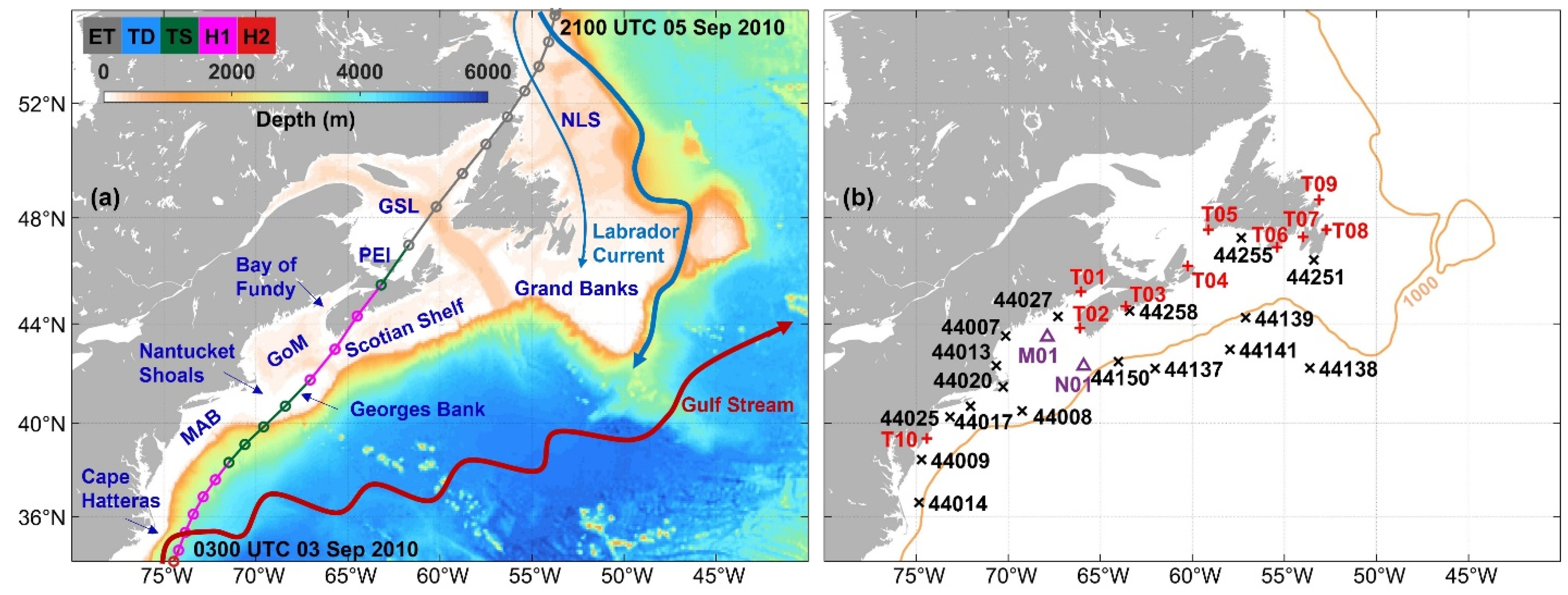
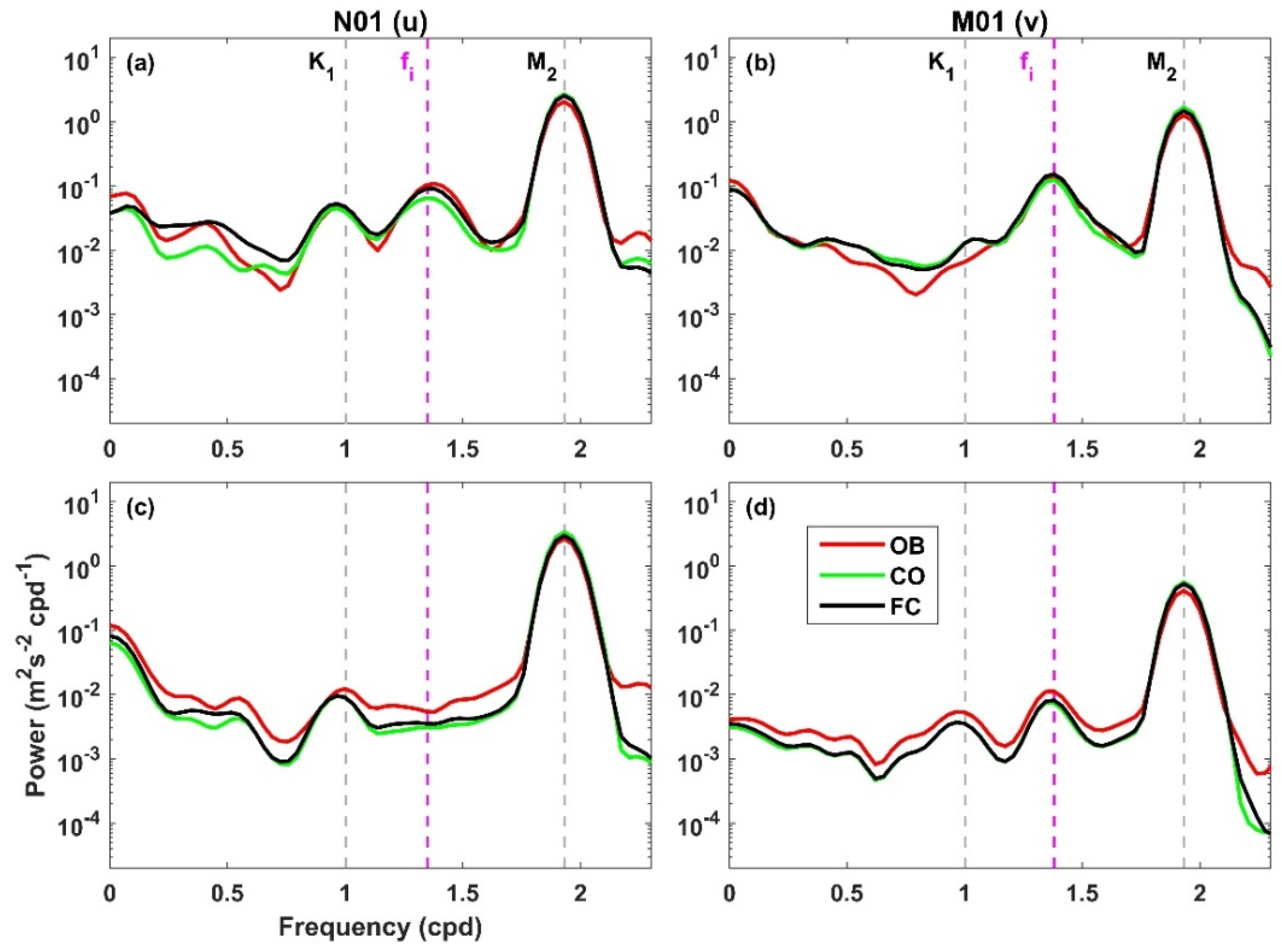
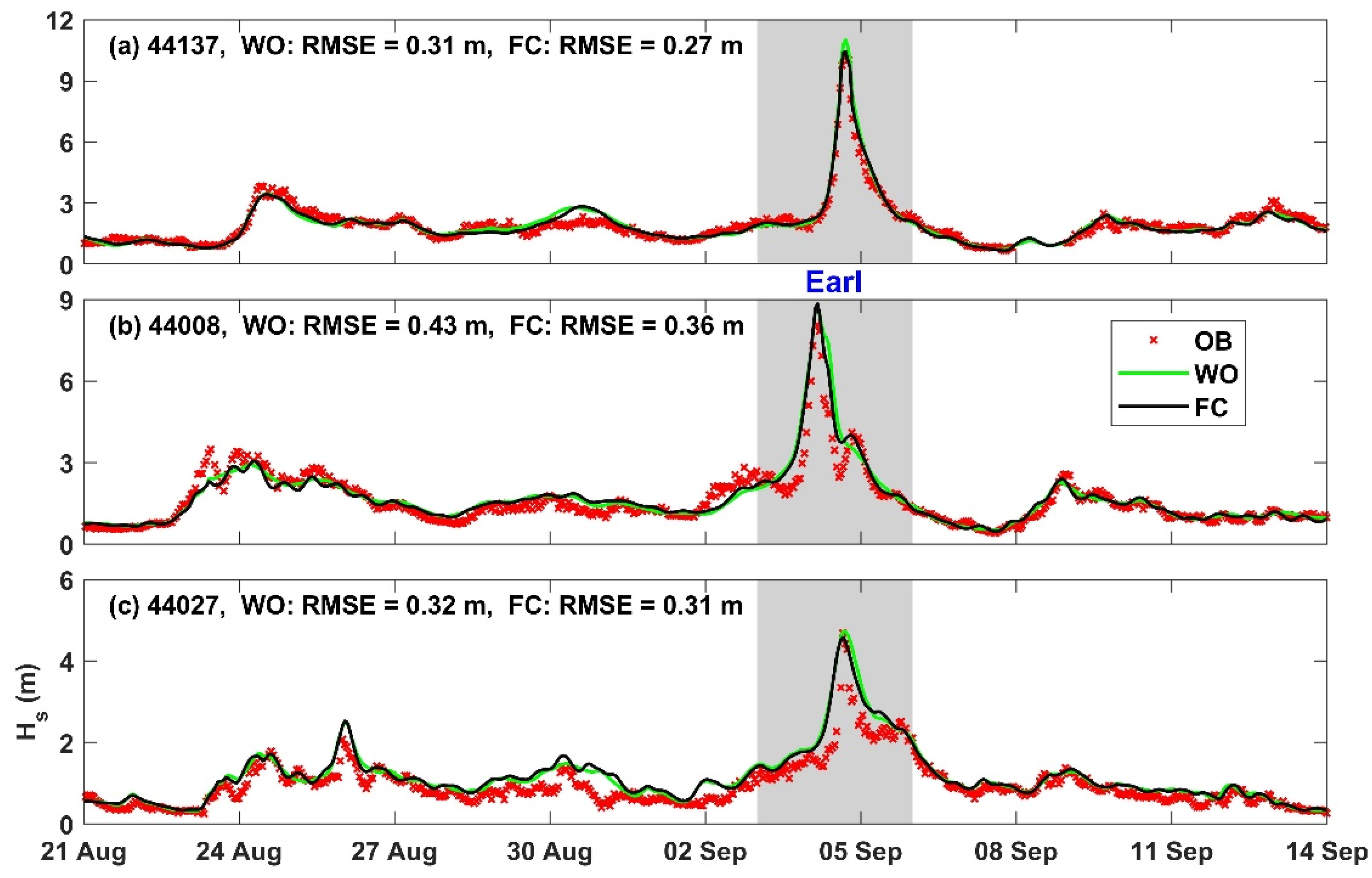
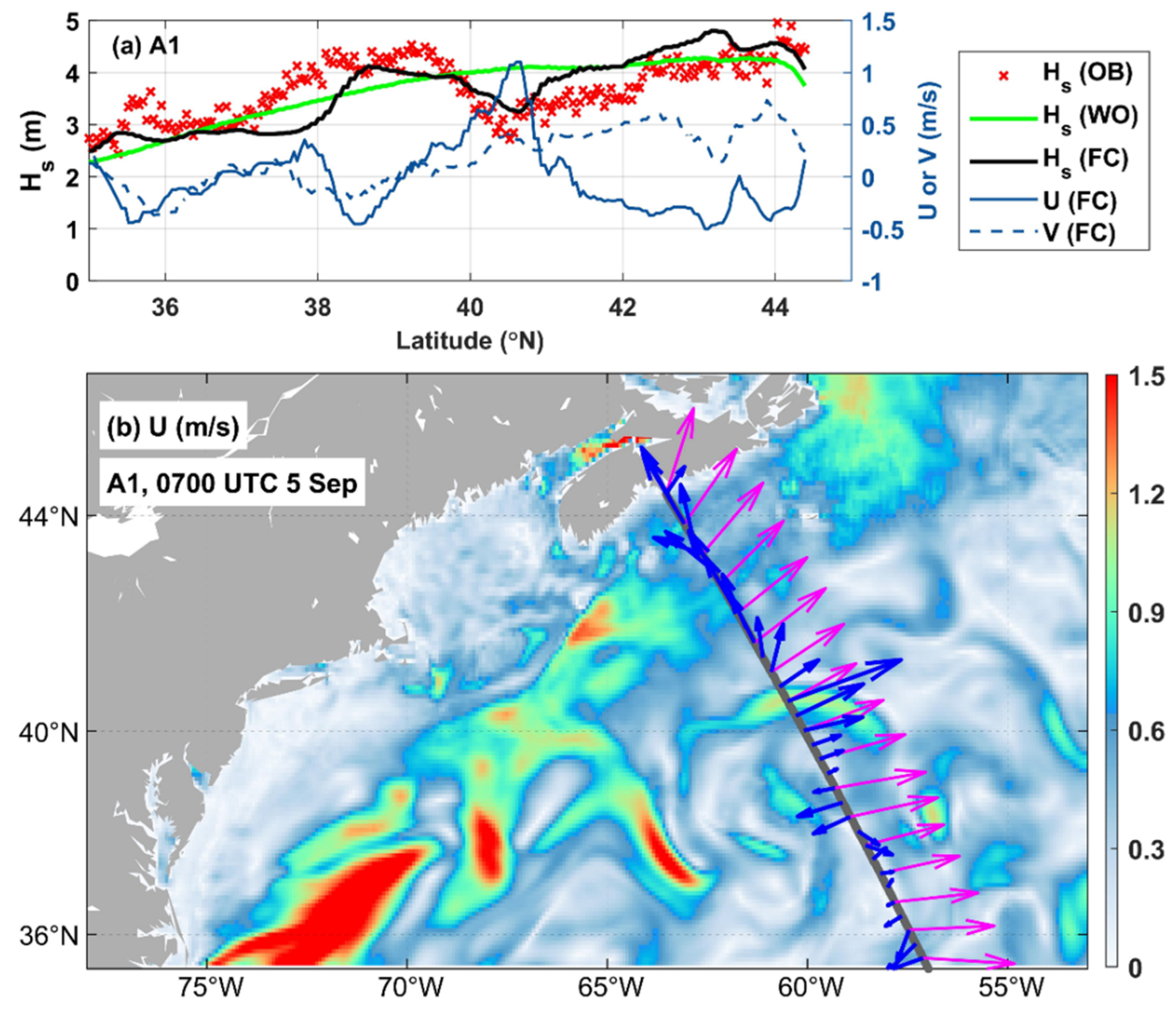
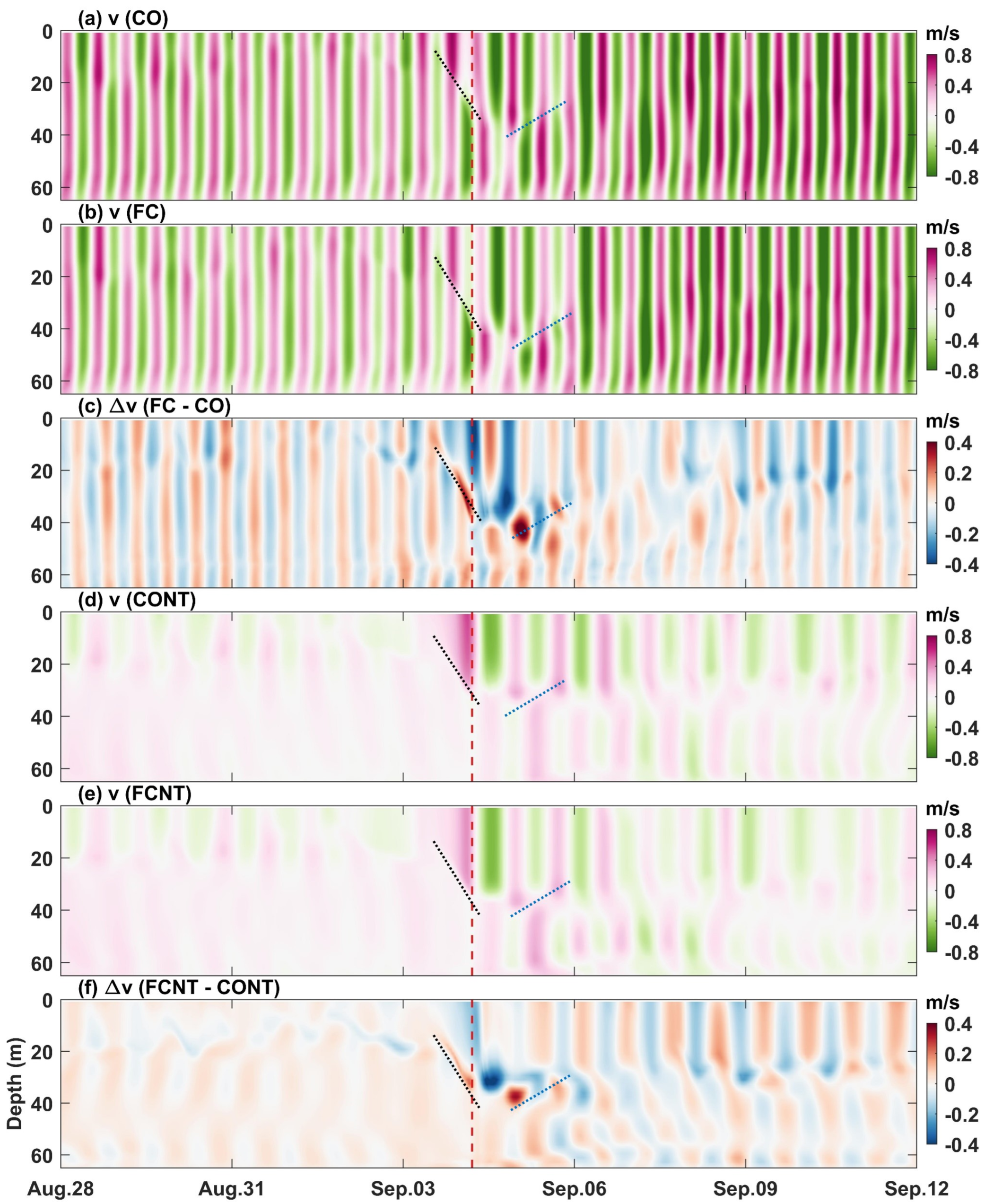
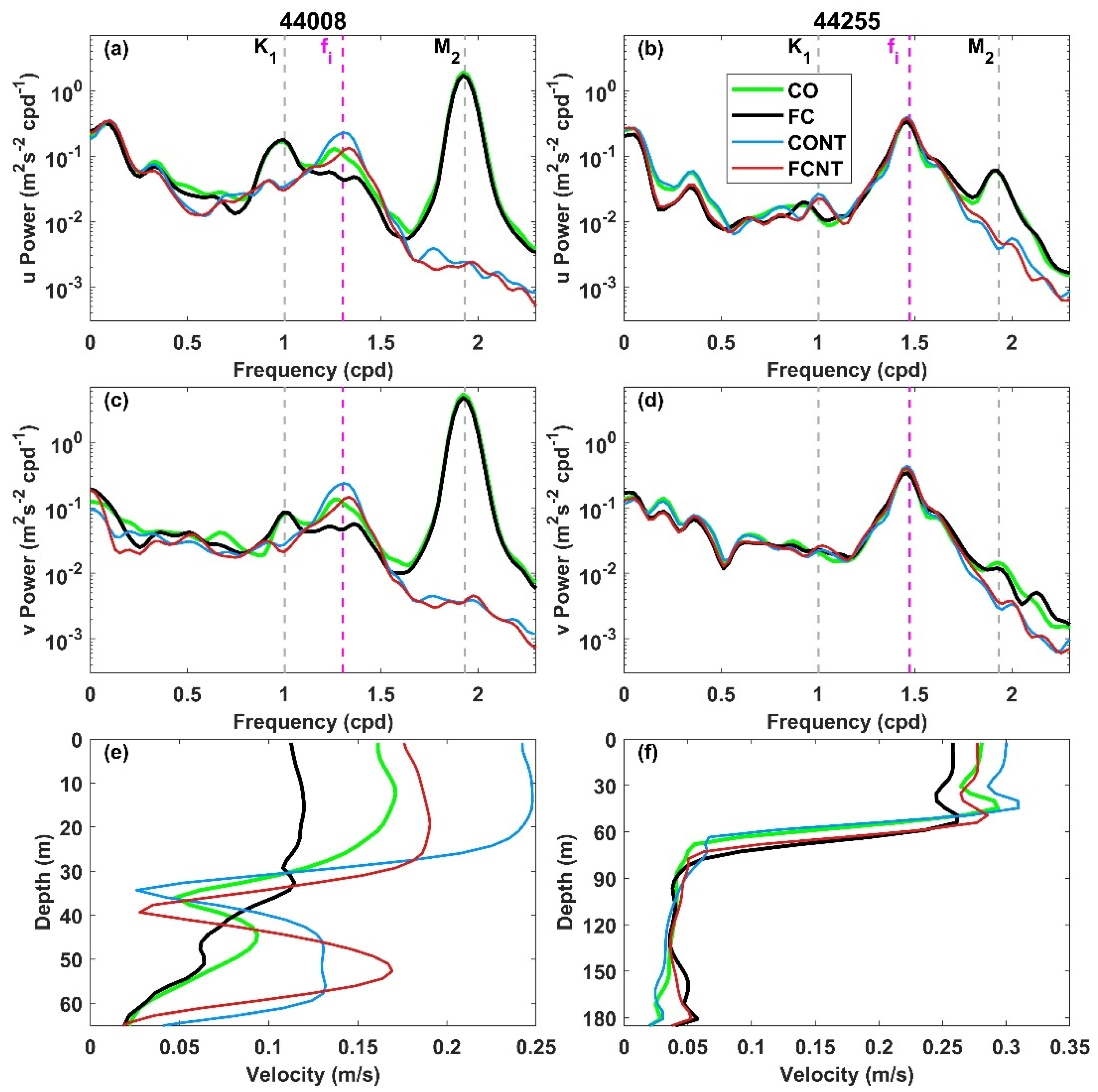
Table 1.
Model configurations for a series of numerical experiments using CWTCM-NWA.
| Run | Description | Wave- Induced Forces | Wave- Enhanced Mixing | Wave- Enhanced Bottom Stress | Wave- Dependent Wind Stress |
|---|---|---|---|---|---|
| WO | Wave-Only model | - | - | - | - |
| CO | Circulation-Only model | - | - | - | - |
| FC | Fully Coupled model | + | + | + | + |
| CONT | Circulation-Only model without tides | - | - | - | - |
| FCNT | Fully Coupled model without tides | + | + | + | + |
| NWF | Coupled model without wave-indued forces | - | + | + | + |
| NVM | Coupled model without wave effects on vertical mixing | + | - | + | + |
| NBS | Coupled model without wave effects on bottom stress | + | + | - | + |
| NWS | Coupled model without wave effects on wind stress | + | + | + | - |
Disclaimer/Publisher’s Note: The statements, opinions and data contained in all publications are solely those of the individual author(s) and contributor(s) and not of MDPI and/or the editor(s). MDPI and/or the editor(s) disclaim responsibility for any injury to people or property resulting from any ideas, methods, instructions or products referred to in the content. |
© 2023 by the authors. Licensee MDPI, Basel, Switzerland. This article is an open access article distributed under the terms and conditions of the Creative Commons Attribution (CC BY) license (https://creativecommons.org/licenses/by/4.0/).
Share and Cite
MDPI and ACS Style
Lin, S.; Sheng, J. Interactions between Surface Waves, Tides, and Storm-Induced Currents over Shelf Waters of the Northwest Atlantic. J. Mar. Sci. Eng. 2023, 11, 555. https://doi.org/10.3390/jmse11030555
AMA Style
Lin S, Sheng J. Interactions between Surface Waves, Tides, and Storm-Induced Currents over Shelf Waters of the Northwest Atlantic. Journal of Marine Science and Engineering. 2023; 11(3):555. https://doi.org/10.3390/jmse11030555
Chicago/Turabian StyleLin, Shangfei, and Jinyu Sheng. 2023. "Interactions between Surface Waves, Tides, and Storm-Induced Currents over Shelf Waters of the Northwest Atlantic" Journal of Marine Science and Engineering 11, no. 3: 555. https://doi.org/10.3390/jmse11030555
Note that from the first issue of 2016, this journal uses article numbers instead of page numbers. See further details here.