
Correction of Temperature from Infrared Cameras for More Precise As-Is 3D Thermal Models of Buildings

1
3D Visual Computing & Robotics Lab, University of Castilla-La Mancha, 13071 Ciudad Real, Spain
2
Department of Civil and Building Engineering, University of Castilla-La Mancha, 13071 Ciudad Real, Spain
3
Department of Applied Mechanics and Project Engineering, University of Castilla-La Mancha, 13071 Ciudad Real, Spain
*
Author to whom correspondence should be addressed.
Appl. Sci. 2023, 13(11), 6779; https://doi.org/10.3390/app13116779
Submission received: 5 April 2023
/
Revised: 18 May 2023
/
Accepted: 30 May 2023
/
Published: 2 June 2023
(This article belongs to the Special Issue New Insights into Heat and Mass Transfer)
Abstract
:Featured Application
The corrections presented in this paper can be applied in order to obtain a reliable empirical calculus of energy parameters in buildings by means of infrared imaging techniques.
Abstract
This paper studies how to create precise 3D thermal maps of building interiors by correcting the raw apparent temperature values yielded by the thermal cameras. This matter has not, to date, been dealt with in the literature, which leads us to conclude that the current methodologies that obtain thermal point clouds are incomplete and imprecise. Without a suitable correction, any further energy parameter calculation obtained from the thermal point cloud is incorrect. This paper presents a method that deals with important aspects to be corrected, such as the repeatability of thermal cameras, the use of the true emissivity of the materials sensed, and the inclusion of the reflected radiant energy caused by the environment. The method has been successfully tested in several indoor scenes using a thermal scanning platform. The results show that significant corrections of up to 8% of the raw temperature values must be carried out in the final thermal model, thus justifying the need for the correction. As an application of the method, an empirical calculation and a comparison of transmittances with and without temperature corrections are presented at the end of the paper. In this case, the relative errors with respect to the average nominal U-value decrease from 94% to 11%. The general conclusion is that precise calculations of energy parameters in which infrared cameras are involved must take these corrections to temperature into account.
1. Apparent Temperature in 3D Thermal Point Clouds
Papers advising the insertion of thermal data into building information models (BIMs) and digital twins of buildings have appeared more frequently in the last 5–10 years [1,2,3,4,5]. Nevertheless, thermal point clouds (TPC) have recently been included in papers and conferences as a new challenging topic with tremendous potential in future applications in architecture, engineering and construction (AEC). In this environment, the term “as-is” 3D thermal model has been adopted as a record of the geometric and thermal measurements of an existing building at a specific time. These measurements are synthesized into a scalar geometric model, in which a point in the space has an assigned temperature. When compared with 2D thermographs, which provide a very limited and partial thermal representation of a building [4], TPC platforms yield integrated 3D geometry and temperature, which can later be extended to building energy models (BEMs) [6].
Very few works have appeared in the field of mobile thermal scanning platforms to date. The existing platforms concern terrestrial robots or unmanned aerial vehicle (UAV) platforms [6,7,8,9,10,11] which, with a greater or lesser extension, collect thermal data from the indoors or outdoors of buildings. In all these works, the temperature provided by the infrared camera, which is later inserted into each of the points of the TPC, is not corrected as regards different factors that affect the temperature value. Therefore, it is possible to state that these TPC are, in some respects, incorrect.
When employed in a three-dimensional environment, thermal data are obviously obtained using thermal cameras. It is, therefore, necessary to include aspects regarding the errors and corrections of these infrared cameras, which are later included in the point clouds. Unfortunately, no previous work had dealt with the calibration of temperature in IR cameras when specifically applied to thermal point clouds. Apart from intrinsic calibration procedures, such as radiometric, blackbody and geometric distortion calibrations, some sort of extrinsic calibration must be carried out before considering that the apparent temperature provided by the IR camera is true. It is well known that the accuracy of IR cameras depends, to a greater or lesser extent, on the following factors: the correct emissivity of the objects; the distance to and orientation of the surface measured [12]; the repetitiveness of temperature in successive shots, or the temperature of the circuits of the camera. A brief reference is made to the studies that deal with some of these noise sources in the following paragraphs.
Some authors discuss the radiometric calibration of thermal cameras used together with SfM (structure from motion) digitization techniques and the geometric reconstruction of point clouds obtained using depth images. For example, Lin et al. [13] deal with two problems that should be considered when calibrating thermal cameras. These are temporal non-uniformity, which refers to the changes produced in the irradiance of the object, along with the temperature of the sensor that is dependent on time, and spatial non-uniformity, which is caused by the different responses in the pixels of the CCD (charge coupled device). In this respect, the authors of [14] present a thermal camera that allows the adjustment of different factors concerning the temperature and ambient humidity. However, they point out that these have relatively little effect in the case of close-range applications, with building facades not exceeding 26 m in height and continuous facade lengths of up to 100 m. The paper by Zhu et al. [15] comprises a study concerning the thermal inaccuracies that occur in cameras that are used to perform videogrammetry. A plane displacement function is proposed in order to adjust the temperatures measured, and several tests are subsequently carried out with different orientations of the camera so as to avoid the thermal drift caused by movement. A similar method is proposed in [16]. This system uses a beam splitter together with a convex lens and a photographic mask, all of which compensate for the thermal instability of the camera. In [17], the authors deal with the geometric distortion of 2D images but do not consider other sources of noise in the thermal calibration. In their work, Malmivirta et al. [18] perform a blackbody calibration and then apply a calibration technique based on deep learning. This method is able to minimize internal thermal changes within the camera. It is particularly useful in applications that require continuous thermal measurement, in which the camera tends to overheat during use. In [19], several experiments are carried out with a handheld camera and a UAV (unmanned aerial vehicle), showing how the temperature measured with the sensor varies and takes up to 60 min to stabilize, which adds complexity to the measurement procedure.
Although it can be considered a current issue, there is hardly any literature on the subject of the variability and correction of the temperature of IR cameras when used to create 3D thermal clouds inside buildings. The objective of this paper is, therefore, to show an automatic correction procedure that eventually yields a more reliable 3D thermal model of the scene.
2. An Overview of the Approach
A thermal camera detects a mixture of radiant energy with contributions originating from the sensed object, the object’s surroundings (reflection) and the atmosphere (ambient). All these radiant contributions determine the total radiation power incident on the detector and, therefore, the temperature value provided by the camera. Many other parameters also affect the IR images generated by the detector inside the camera to a greater or lesser extent. Some of these are the following: the temperature of the external optics of the camera, the instability of the camera, the emissivity of the sensed object, the distance from the camera to the object, the observation angle and the size of the object.
Our context is that of the indoors of buildings in standard conditions, in other words, scenarios with short distances, low camera observation angles, non-extreme relative humidity, non-extreme interior temperature and good insulation. Factors such as distance from the camera to the object, observation angle, relative humidity, ambient temperature and atmospheric temperature are not, therefore, included in our research. However, apart from the black body calibration, which is conducted only once before using the thermal camera, we have considered the following important aspects: the temperature of the optics and electronic circuits of the camera, the emissivity of the sensed object and external radiation. These factors have a clear influence on the temperature value yielded by the IR camera.
The correction of the original temperature (i.e., provided by the camera) is performed in two stages. In the first stage, we deal with the factors related to problems concerning the camera becoming hot and the effect of repetitiveness, which generate the apparent temperature. This aspect is presented in Section 3. Factors that are external to the camera, such as the emissivity of the object and external radiation, are discussed in Section 4, in which we also show how the real temperature is obtained. In order to show an application of our method, Section 5 deals with the empirical estimation of the transmittance (U-value). A representative test carried out in a case study is presented in Section 6. Temperatures before and after successive corrections are compared, and the calculation of the respective transmittance values on two walls are also shown. Finally, the conclusions of the work are presented in Section 7.
3. Stage I: Dealing with the Repeatability of the Thermal Camera: The Apparent Temperature
When creating a thermal point cloud, one of the problems that arise is the variability in the temperature of the thermal camera, an issue that has been ignored in virtually all the references discussed in Section 1, with the exception of [18,19]. However, although the most recent related references were published in 2021, signifying that it can be considered a current issue, hardly any other literature on thermal data and its accuracy, when applied to the creation of 3D thermal clouds inside buildings, has appeared in the last year.
In our case, the effect of the variability or repeatability of infrared cameras means that the temperature value of the same pixel for shots with the same viewpoint separated by a short interval of time (seconds) can vary appreciably. It may also mean that adjacent thermal images in a full revolution of the IR camera have significant and inconsistent global temperature gradients. The eventual effect of this random variation is that the thermal cloud lacks the temperature precision required and has thermal inconsistencies in space. Examples of these variations will be provided in Section 5.
In order to correct this problem, a single scanner measurement (3D coordinates) but with a number n of consecutive thermal images of the same viewpoint of the scene are taken. In our system, this entails the system performing n complete turns (usually from 6 to 10) of 360º, taking 10 thermal frames in each turn. These data are then used to carry out a statistical procedure for the n frames corresponding to each camera rotation, in which atypical images that we denominate as outliers will certainly be identified. The pseudocode of the outlier image filtering algorithm is shown in Algorithm 1.
The thresholds Up1 and Up2 have been established by means of empirical procedures after testing the results on 260 images. The value of Up1 follows the criterion of a Matlab function that detects outliers in a dataset. This function returns true for all elements (in this case, images) with more than three standard deviations from the mean. The value of Up2 has been established as 3% of the total number of pixels in the image.
| Algorithm 1: Algorithm for the detection of outlier images and the creation of valid average thermal images. |
| Inputs: a × n Ir_images: (a = number of sessions, n = number of camera positions) Pixel_Threshold: Maximum deviation with respect to the variance: Image_Threshold: Maximum percentage of outlier pixels in : % Do for each session of the Ir_camera. FOR i = 1 TO a % Do for each pixel (x,y) of FOR 0 < x < dimx & 0 < y < dimy Temperature array assigned to (x,y) → % Do for each position of the Ir_camera FOR j = 1 TO n % Label a pixel (x,y) in as valid (0) or outlier (1): → IF ELSE END END END % Do for each position of the Ir_camera FOR j = 1 TO n % Label as valid or outlier IF is valid ELSE is outlier END % Obtain the average thermal image of the i-th position of the Ir_camera and valid) END |
This algorithm evaluates whether or not an image is classified as an outlier within a set of n images that should, in theory, be very close in terms of pixel temperature. This process is first based on the labelling at a pixel level, whereby each pixel in each image is labelled as an outlier pixel or as a valid pixel. Depending on the percentage of the outlier pixels in an image, the image is ultimately labelled as an outlier image or as a valid image. After performing this process, an average image is generated with the set of valid images. The temperature contained in this average image will, from here on, be denominated as the apparent temperature.
4. Stage II: Obtaining the True Temperature of an Object
From this point on, a surface of any structural element that has been recognised in the point cloud model of the scene will be denominated as an “object”; that is, the object classes are the following: the structural element (SE) (floor, ceiling and wall), the window frame or the door frame. It will, in turn, be assumed that a scene or zone will consist of a standard room (with doors and windows).
We shall additionally assume that the thermal point cloud has been corrected for the repeatability effect (as shown in Section 3) and that it has been segmented into points corresponding to the floor, ceiling and each of the walls. We initially created a raw 3D point cloud in which each point has four associated values (RGB + Temperature). This point cloud is then segmented into smaller point clouds corresponding to the floor, ceiling and each of the walls. Orthoimages are subsequently obtained by projecting each segment from a specific point of view (for example, perpendicular to a certain wall) and creating the corresponding 2D images. The pixel of an image consequently maintains its associated RGB and temperature values. In the first case, we obtain a Colour Orthoimage (CO), and in the second, a thermal orthoimage (TO), which contains apparent temperatures. It is also assumed that the thermal camera has worked by default with emissivity one throughout this process.
In this section, the temperatures of the objects contained in a TO are corrected by taking into account the emissivity and radiation effects. From here on, the corrected temperature will be denominated as the real temperature.
Several targets comprising electrical tape and wrinkled pieces of aluminium foil are spread on the existing objects in the scene beforehand. Assuming that the target is a rectangle, the length of the sides of the electric tape and aluminium piece are in the ranges of 4 to 10 and 10 to 20 pixels, respectively, which in real dimensions are of 8 to 20 and 20 to 40 cm. As will be shown in the following subsections, these targets are necessary in order to make corrections derived from the reflected radiation and calculate the real emissivity of the objects.
Let us suppose an object O, detected and delimited in the colour and thermal orthoimages, which belongs to a certain facing on which an apparent average temperature of has been detected. The apparent temperature correction is performed by employing the following steps.
4.1. Step 1: Reflected Apparent Temperature
The reflected apparent temperature can be measured for one or several wrinkled pieces of aluminium foil placed on the object. This region can be delimited in CO when a high-frequency filter is applied to it. The aluminium target is usually placed in the geometric centre of each object (e.g., the centre of a wall). This piece is located automatically by means of a high-pass filter algorithm. This filter makes an image appear sharper and also emphasizes fine details in the image. After applying this filter, the wrinkled piece of aluminium foil will appear in the image as a region with rapid intensity changes within a non-texture background and will be easily detected. If there is more than one target on the surface of an object, the average temperature is calculated.
When the emissivity is fixed to 1, it is assumed that radiation originating from outside or from other SEs is emitted by a diffuse reflector. The assumption of that distance from the camera to the object is ideally 0, thus making it possible to assume a null atmospheric effect. The average temperature of the dual region in T0, , is, therefore, then taken as the valid Reflected Apparent Temperature of object O.
4.2. Step 2: Real Temperature of a Piece of Electrical Tape near the Object O
Since the emissivity of electrical tape is known (), its real temperature can be obtained by means of Equation (2), in which represents the temperature measured by the thermal camera. is again calculated after segmenting the area corresponding to the tape in CO. In this case, a simple colour segmentation algorithm provides the solution. The closest segment to the object O is delimited in CO, and the average temperature corresponding to the dual region in TO is taken as the real temperature of the electrical tape.
4.3. Step 3: Emissivity of Object O
The emissivity of the object O is obtained from Equation (3). In this case, it is necessary to measure the temperature provided by the thermal camera in the proximity of the electrical tape. This can be performed by exploring the temperature of a narrow ring around the tape region detected previously in Step 2. The average temperature in this ring is again defined as the apparent temperature of the region near the object and the tape, .
4.4. Step 4: Real Temperature of Object O
Since it is assumed that the region that covers the complete object O in TO has been calculated beforehand, the average apparent temperature of the object, , is easily obtained. Equation (4) provides the value of the final real temperature of object O.
5. Obtaining Transmittances with Real Temperatures
As an application of our method, the corrected temperatures are eventually used to empirically estimate the transmittance (U-value) of the objects on walls (such as door frames, window frames and wall areas). As will be shown in Section 6.4, the experimentation regarding this approach has been conducted under the recommended premises (following ISO 9869:2014, 2018, [20]) of large and stable indoor-outdoor temperature gradients, and without heating and cooling systems.
It is possible to classify the experimental U-value assessment methods into methods that do and do not employ the heat flux measurement. With regard to the latter method, the temperature-based methods shown in [21] utilise both the indoor surface temperature and the indoor and outdoor ambient temperature in order to calculate the U-value of the walls. As it is considered that the real temperature is attained by using infrared cameras, it is assumed that this can be included as a new thermography-based method that is extended to the 3D dimension. A literature review on infrared thermography (IRT) based methods was performed by the authors of [22], who stated that infrared thermography-based methods are rapid and reliable under certain specific conditions but that the technique must continue to be refined. Many different approaches and formulas with which to calculate the U-value in this context have been published. The formulation appertaining to Jankovic al. [23] has been employed herein, as follows.
The transmittance of an object is defined as the inverse function of the thermal resistance of the object (Equation (5)), which is decomposed into convective and radiative components. Equation (7) corresponds to the convective part of Equation (6), in which the surface convection coefficient is usually taken from a standard tabulated value (normally 7.69 W/m2 °C), whereas and correspond to internal and external temperatures measured by local sensors.
The radiative component of the thermal resistance of the object is calculated from Equation (8). In addition to again containing and , this equation also includes the emissivity of the object, , which is calculated from Equation (3), and the Stefan Wolfman constant 5.67 × 10⁻⁸ W/m2 K4.
6. Experimental Results
6.1. Thermal Scanning Platform
The methodology that performs the temperature correction has been tested in the indoors of buildings composed of several rooms (or zones) using our thermal scanning platform. As a case study, the results obtained for two different zones are shown throughout this section.
The scanning platform, which is composed of a 3D scanner, a colour camera and a thermal camera, makes it possible to generate panoramic thermal point clouds by following a procedure presented in [24]. The scanner scans a space of 360° × 320° (v × h) and has a range of accuracy of 4 mm at 10 m (Z resolution) and 7 mm at 20 m. The resolutions are of 3, 18 and 65 million points for fast, standard and high-density modes, respectively. The fact that it is programmed using its own SDKs makes it possible to customise the data acquisition process.
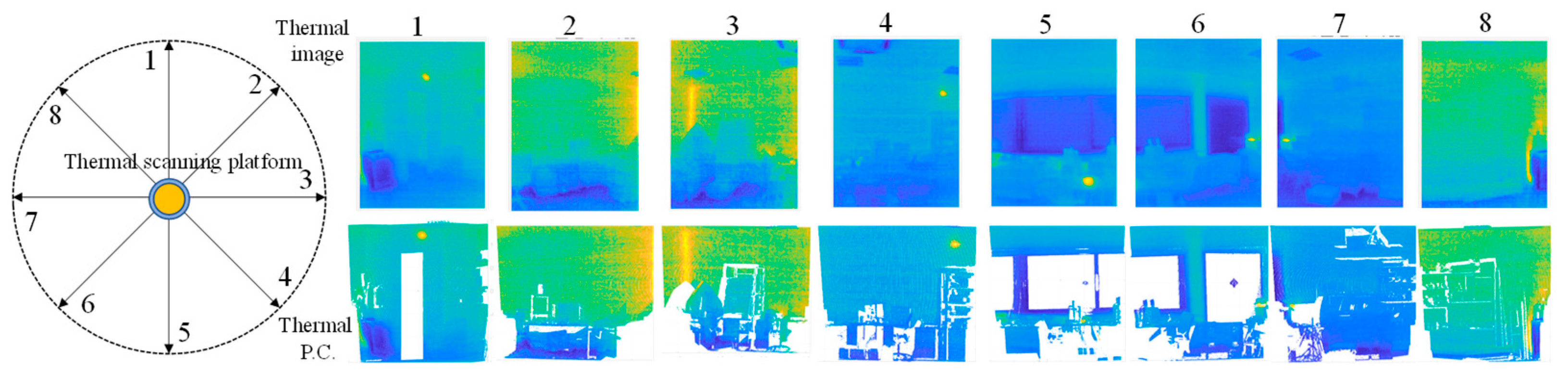
The RGB camera has a resolution of 2592 × 1944 pixels with an FoV of 60° × 45° (V × Hz). The thermal camera takes 10 images of 120 × 160 pixels with a reduced field of view of 71° × 56° (v × h), thus equally covering 360° × 71°. These ten images are subsequently used to assign temperatures to 3D points. It functions in a temperature range of between −10 °C and 65 °C, and its thermal sensitivity is 0.05 °C. Figure 1 shows the assignment of thermal images to 3D points for each IR image in Zone 0 (lab). The thermal image and the portion of the point cloud with the assigned temperature are displayed in pairs.
The platform is programmed under ROS Melodic Morenia on Ubuntu 18.04.05 LTS with C++ and Matlab R2022a scripts.
Apart from the correction processes presented in this paper, the thermal camera has previously been corrected with a black-body device and subsequently calibrated with the help of contact devices with a precision of below 0.2 °C, all of which is performed in order to measure the offset and conversion of the radiance value that the thermal camera provides. This process has been performed with 200 measurements of temperature, obtaining an average precision of 0.06 °C.
6.2. Detecting Outlier Images and Obtaining Average Thermal Images: Results of Stage I
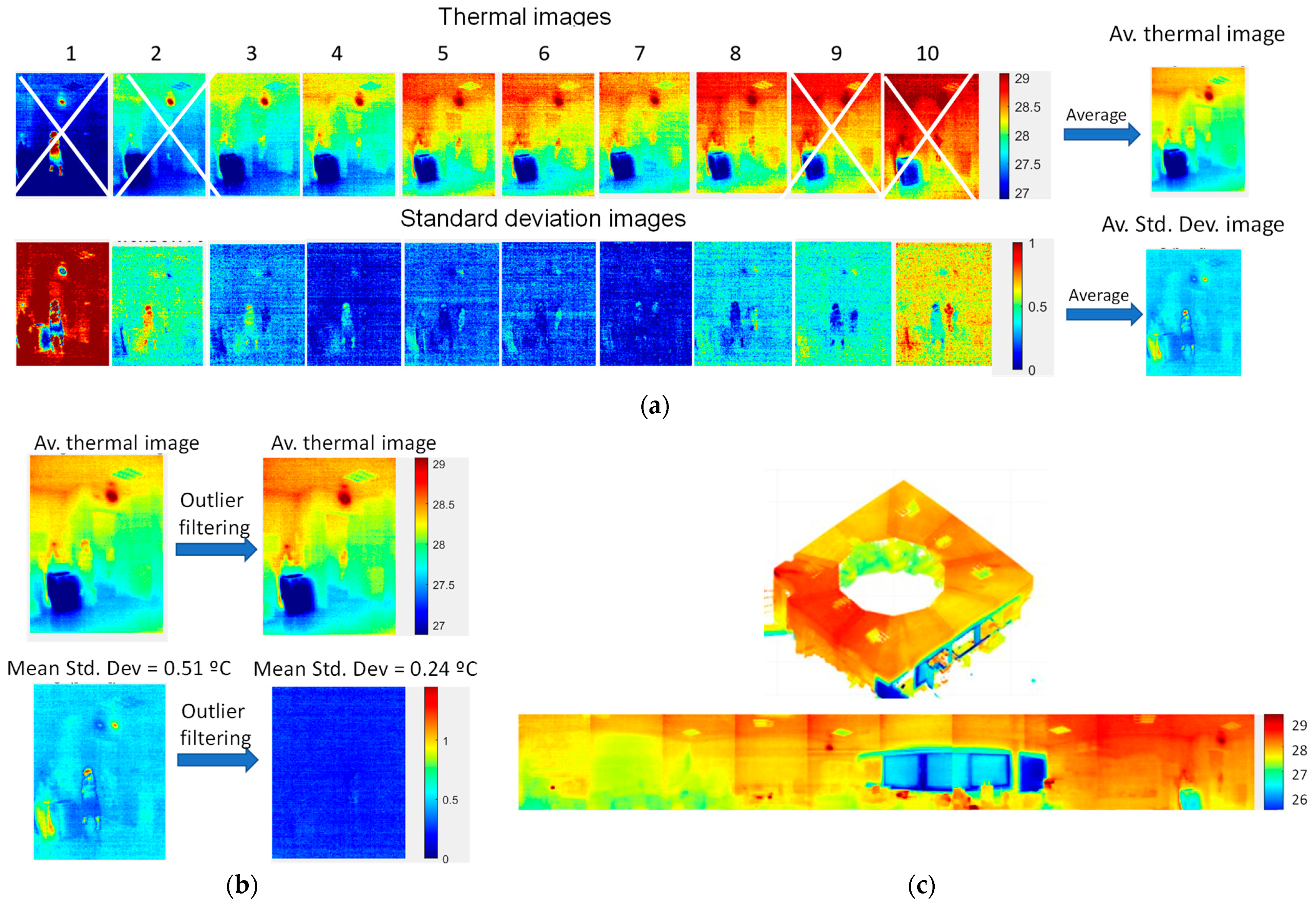
As explained in Section 3, the thermal camera variability issue is solved by repeating thermal images from the same viewpoint and then detecting and removing the outlier images. Figure 2a provides an example of this process. In this case, ten thermal images for the first rotation of the platform are analysed. The discrepancy between the temperatures can be clearly appreciated since it reaches up to 1.5 °C in repetitions 1 and 10. Below are the standard deviation images with respect to the original mean thermal image. In this example, the outlier detection algorithm concludes that images 1, 2, 9 and 10 are outlier images. The average image of repetitions 3, 4, 5, 6, 7 and 8 is, therefore, taken as the corrected and representative thermal image corresponding to the first rotation of the thermal camera. Figure 2b presents the average original and standard deviation images before and after carrying out the outlier image filtering process. As can be seen, the average standard deviation image now has a mean value of 0.24 °C, which is a considerable improvement to the earlier value of 0.51 °C. The average image will later be used to calculate a partial thermal cloud corresponding to the first rotation of the platform.
The same process is carried out for the images corresponding to the remaining nine rotations, thus obtaining the corresponding ten partial thermal point clouds. Note that the temperatures contained in these average thermal images are apparent temperatures that will later be corrected with the calculated emissivity and the reflected radiation effects. Figure 2c shows a composition containing all the apparent temperature images, presented as a panoramic image, and the apparent thermal cloud calculated with them.
6.3. Obtaining Real Temperatures: Results of Stage 2
The apparent thermal point cloud (ATPC) is used to calculate the real thermal point cloud (RTPC). As mentioned in Section 4, the ATPC is segmented into points belonging to the walls, ceiling and floor (assuming that the scene is a standard room), and the corresponding colour orthoimages (COs) and apparent thermal orthoimages (ATOs) are obtained automatically.
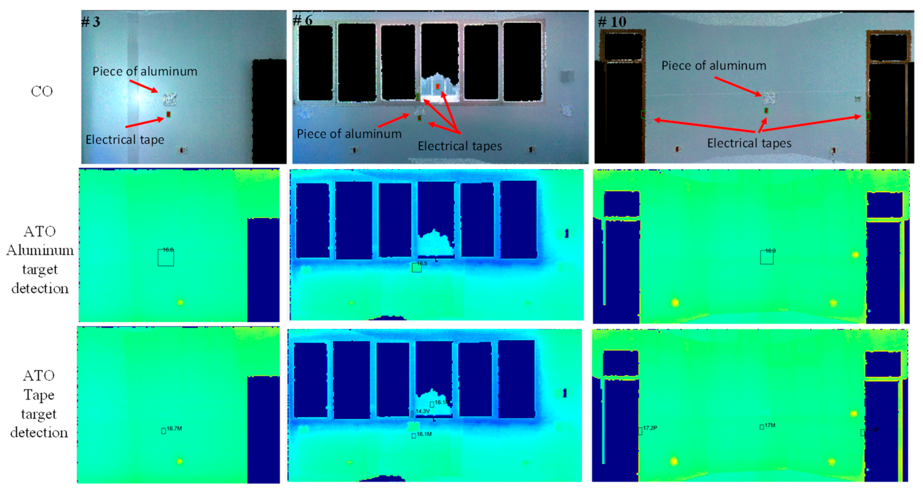
Upon processing COs and ATOs, as explained in the four steps shown in Section 4, the real thermal orthoimages are eventually obtained. Figure 3 illustrates the COs and TOs corresponding to SEs #3, #6, #9 and #10 of Zone 1 (Room East1), in which wrinkled pieces of aluminium foil and electrical tape have been placed on four faces of the room. All these targets are automatically recognised and delimited in the COs. The dual ATOs are then used to first calculate the reflected apparent temperature by means of Equation (1). The real temperatures of pieces of electrical tape near a door frame (if any), a window frame (if any) and wall areas are calculated according to Equation (2). Figure 4 shows how the aluminium foil and electrical tape targets are automatically detected. The emissivity of the objects “window frame”, “door frame” and “wall area” is obtained from Equation (3) using the mean temperature of narrow rings around the corresponding targets. Finally, the real temperatures of all the objects are calculated using Equation (4).
Table 1 shows the values of the apparent and real temperatures measured on the aluminium foil (T) and the electrical tape targets (AT and RT) on all the walls in the scene, which are denominated as structural elements (SE). As can be seen, SE # 10 contains two doors, and SE # 6 contains windows. In general, it is possible to state that increases of less than 0.2º are detected between the apparent and the real temperatures of the targets.
Table 2 presents the correction of temperatures for the objects “door-frame”, “window-frame” and “wall-area” for each of the SEs of the room. Differences of up to 0.41 °C can be observed in this case. While differences for door frames are insignificant, window frames and especially the wall areas yield greater differences in the range of from 0.1 to 0.4 °C.
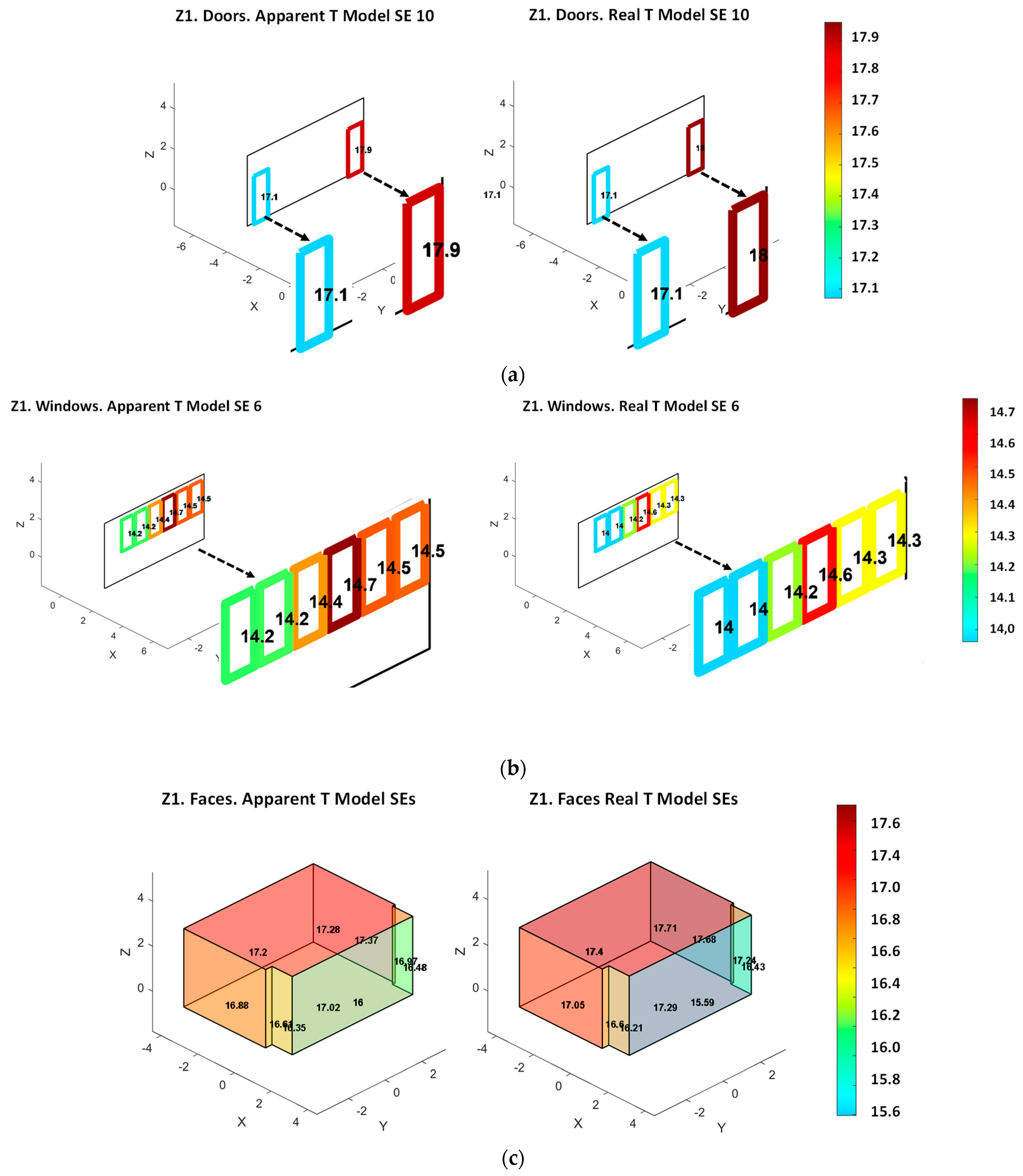
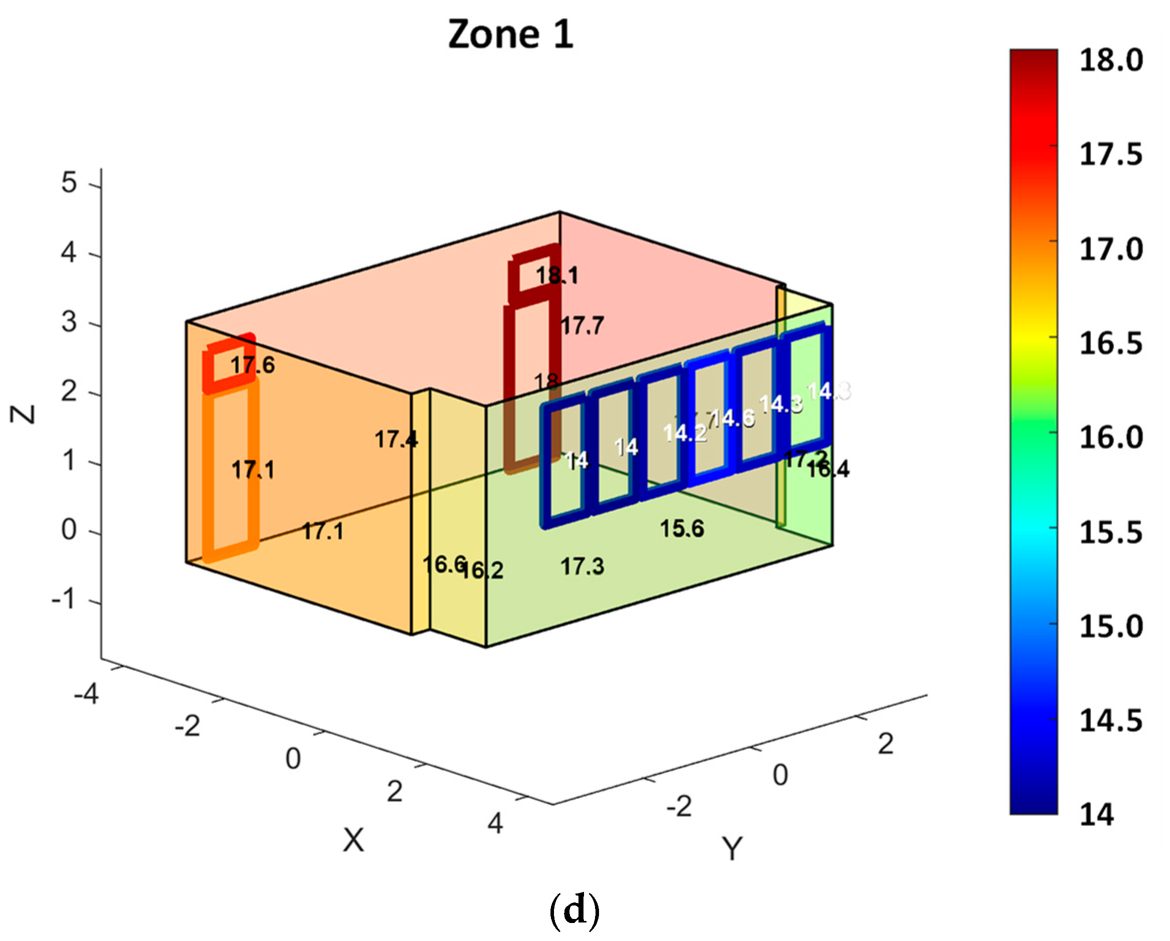
Finally, Figure 4 illustrates the correction of the temperature before and after performing the correction of temperature explained in Section 4. Figure 4a,b show the results for doors in SE #10 and windows in SE #6, whereas Figure 4c represents the thermal model that includes the faces corresponding to the floor, ceiling and walls. Figure 4d shows the final corrected model with all the objects and assigned temperatures.
In order to better visualize the differences in temperature, we show the simplified thermal model in which the average temperature is assigned to each object class. Moreover, the range of the colour code for each part of Figure 4 has been fitted to the minimum and maximum temperature, thus allowing the differences between apparent and real temperatures to be clearly seen. Note that both the wall areas and the external window-frames undergo the highest correction.
6.4. Total Temperature Variations
Table 3 summarizes the results obtained for the variation in temperature for the aforementioned objects after considering the corrections from Stages I and II. In this table, we consider the variations between original vs. apparent temperatures (|ΔI|) and apparent vs. real temperatures (|ΔII|). The third column is the total sum of both corrections (|Δtotal|). The row below each structural element corresponds to the contribution (percentage) of each specific correction.
It is clear that the first correction has the greatest impact on the final temperature, achieving a total average impact of 62.1%, whereas the second factor covers 37.9% of the total variation. The quality of the measurements that the infrared camera provides is, therefore, the main issue to be minimized. Overall, the corrections are in the range of 0.07 °C to 1.11 °C, which signifies a variation with respect to the original temperature provided by the infrared camera of up to 7.9%.
6.5. Calculation of Transmittances
As an example of the application of our approach, we present the results obtained when estimating the transmittance, which is an indoor surface heat transfer coefficient, on the basis of experiments carried out on two walls of a building. Although the transmittance is usually in the range of 1.5–2.5 W/m2K, without insulation, we expected to attain values in the range of 0.1–0.5 W/m2K, as occurs in most of the buildings in Europe.
As is already known, U-values are obtained by employing a large variety of empirical methods, but some authors [26,27] consider that certain energy parameters, such as the surface heat transfer coefficient, cannot yet be estimated at a reasonable level of uncertainty. Estimations are in the range of 60% for instantaneous values, while this decreases to an average of 12–20% for 8-h and always increases for low-temperature gradients. Furthermore, there is a relevant impact on the overall uncertainty of the U-value with sensor quality. In our case, this refers to the thermal camera used in the experimentation.
Lastly, ISO 9869-2:2018, 2018 provides a standardized method that incorporates infrared imaging into the on-site, experimental assessment of U-values on the walls of buildings. This method is limited to walls with a low thermal mass, and measurement campaigns span several days, during which only night-time measurements are used for calculation. However, some authors state that a reliable value of the U-value can be extracted in short measurement times [28].
Our experiments were conducted on the first floor of the Business Incubator Centre Building at the University of Castilla La Mancha by following the U-value measurement guidance, which requires a relevant (large and stable) indoor-outdoor temperature gradient (following [20]). Moreover, the measurements were performed without heating and cooling systems. The U-values were calculated for the objects “window-frames” and “wall areas” of the structural elements #SE6 of Zone 1 (East01) and #SE11 of Zone 5 (Weast02). These are two exterior structural elements with different orientations (east and west, respectively). In all cases, we took 5-h average values with indoor-outdoor gradients of around 10 °C.
The constructive and thermal characteristics that constitute these spaces correspond to the standards for the place and the date of construction of the building. The first and fourth columns of Table 4 present the average nominal transmittances (Ut) corresponding to the window-frames and wall areas of this building, which must be taken as approximate values. This information is included merely in order to evaluate the variation with respect to the empirical values computed from Equations (5)–(8).
The results obtained when using the original temperatures provided by the thermal camera are shown in the columns denoted as Uo. In this case, Equations (1)–(4) were omitted, and the variable T_(object_r) was replaced with the original temperature (that provided by the thermal camera) without correcting Equation (7). In addition, for these cases, the standard emissivity of materials similar to existing ones were taken, in our case, aluminium (window-frames) and plaster (wall area). Column Uc corresponds to the U-values calculated after making corrections I and II. Finally, relative errors Eo and Ec with respect to the nominal values are included.
These results show a significant variation in the empirical U-values without and with the correction proposed in this paper. It is clear that the relative errors decrease when corrections I and II are carried out.
7. Conclusions
The objective of this paper is to show a methodology that corrects the apparent temperature provided by a thermal camera which, together with a 3D scanner, generates the thermal point cloud of an indoor scene. As shown in Section 1, this problem has not yet been properly dealt with in the current literature, and it is, therefore, possible to conclude that the few works focused on obtaining thermal clouds in buildings provide apparent temperatures.
The difference between the apparent temperature and the real temperature of objects in the construction field (i.e., walls, floors, ceilings, doors and windows) is conditioned by multiple factors and may be significant. In our tests, the specific original temperature values provided by the thermal camera have been corrected by up to 1.5 °C (with an average of 0.47 °C) from the original data captured by the thermal camera.
This paper proposes an automatic temperature correction approach that covers the most important effects in our framework. We specifically address variations owing to the internal effects of the IR camera, which lead to an uncontrolled variability in temperature, the calculation of the real emissivity of the objects and the reflected radiation effect. The experimentation carried out in order to test the method shows that, particularly in the case of the first effect, and to a lesser extent in that of the remaining two, the temperature correction is necessary. This is particularly the case if the eventual objective is to calculate quantitative measures of energy parameters, such as transmittance and others.
Several experimental tests have been presented using 3D thermal point clouds taken from a 3D thermal digitizing platform. This system provides dense thermal point clouds that facilitate more reliable average temperature values than mere point temperature records. All this has allowed us, in a first step, to undertake thermal frame filtering procedures, thus improving the quality of the measurement provided by the thermal camera. Furthermore, the dense information contained in the data clouds obtained has allowed us to carry out image processing techniques on the thermal orthoimages, detecting and delimiting objects on the walls in the scene. These techniques were then used to carry out a second correction.
As shown at the end of the paper, the inclusion of an application regarding the empirical calculation of the transmittance of several existing objects on a wall could be extended to other energy parameters in which a reliable temperature value is required and that is obtained from infrared cameras. In the case study described, it will be noted that there is an improvement in the values obtained after making the corrections presented.
8. Limitations and Future Work
This paper proposes an automatic temperature correction approach that requires very robust algorithms in the stages concerning the detection of aluminium and electric tapes. This image processing stage could fail in the case of textured and inhabited indoor buildings. Another disadvantage is that, owing to the fact that the thermal camera variability issue is solved by repeating thermal images from the same viewpoint and then detecting and removing the outlier images, the data-collection stage takes quite a long time, and a larger volume of data is obtained when compared to single sessions.
This work will be improved in the coming months. In the first place, we aim to extend the experimentation carried out with the method for scenes with more extreme temperature ranges, which will be both low (below 5 °C) and high (above 30 °C), and the temperature correction is expected to be much higher. Moreover, we intend to attain a higher degree of automation throughout the process, especially as regards the creation of thermal orthoimages of walls and the recognition and assignment of the average temperatures of the objects detected.
The future developments of this research will lead us to provide a more precise thermal characterisation of the indoors of buildings by using automatic hardware and software tools. On the one hand, the use of robotics platforms will allow us to accomplish thermal scanning sessions without human interaction, thus reducing time and gaining accuracy. On the other, more efficient and robust algorithms that process higher amount of data will be necessary for larger scenarios.
Author Contributions
Conceptualization, A.A., V.P. and F.J.C.; methodology, V.P and F.J.C.; software, A.A.; validation, A.A. and A.R.; formal analysis, A.A.; investigation, V.P. and F.J.C.; resources, A.R.; writing—original draft preparation, A.A.; writing—review and editing, A.A.; visualisation, A.A.; supervision, A.A.; funding acquisition, A.A. and F.J.C. All authors have read and agreed to the published version of the manuscript.
Funding
This research was funded by the European Regional Development Fund (SBPLY/19/180501/ct) and the Ministry of Science and Innovation (PID2019-108271RB-C31).
Institutional Review Board Statement
Not applicable.
Informed Consent Statement
Not applicable.
Data Availability Statement
Not applicable.
Conflicts of Interest
The authors declare no conflict of interest.
References
- Dinis, F.M.; Poças Martins, J.; Guimarães, A.S.; Rangel, B. BIM and Semantic Enrichment Methods and Applications: A Review of Recent Developments. Arch. Comput. Methods Eng. 2021, 29, 879–895. [Google Scholar] [CrossRef]
- Gisbert, F.; Bono, V.; Luis, J.; Soriano, C.; Fiel, V.; Abad, V. State of the art of thermal modelling of buildings from point clouds and infrared thermography. In Proceedings of the 25th International Congress on Project Management and Engineering, Alcoi, Spain, 6–9 July 2021; pp. 6–9. [Google Scholar]
- Wysocki, O.; Xu, Y.; Stilla, U. Unlocking point cloud potential: Fusing MLS point clouds with semantic 3D building models while considering uncertainty. In Proceedings of the ISPRS Annals of the Photogrammetry, Remote Sensing and Spatial Information Sciences, New York, NY, USA, 11–14 October 2021; Volume 8, pp. 45–52. [Google Scholar]
- Hou, Y.; Chen, M.; Volk, R.; Soibelman, L. Investigation on performance of RGB point cloud and thermal information data fusion for 3D building thermal map modeling using aerial images under different experimental conditions. J. Build. Eng. 2022, 45, 103380. [Google Scholar] [CrossRef]
- Qureshi, A.H.; Alaloul, W.S.; Manzoor, B.; Saad, S.; Alawag, A.M.; Alzubi, K.M. Implementation Challenges of Automated Construction Progress Monitoring Under Industry 4.0 Framework Towards Sustainable Construction. In Proceedings of the 2021 Third International Sustainability and Resilience Conference: Climate Change, Sakheer, Bahrain, 15–16 November 2021; IEEE: New York, NY, USA, 2022; pp. 322–326. [Google Scholar]
- Borrmann, D.; Nüchter, A.; Dakulović, M.; Maurović, I.; Petrović, I.; Osmanković, D.; Velagić, J. A mobile robot based system for fully automated thermal 3D mapping. Adv. Eng. Inform. 2014, 28, 425–440. [Google Scholar] [CrossRef]
- Adán, A.; Prieto, S.A.; Quintana, B.; Prado, T.; García, J. An Autonomous Thermal Scanning System with Which to Obtain 3D Thermal Models of Buildings. In Advances in Informatics and Computing in Civil and Construction Engineering; Springer International Publishing: Berlin/Heidelberg, Germany, 2019; pp. 489–496. [Google Scholar]
- Westfeld, P.; Mader, D.; Maas, H.G. Generation of TIR-attributed 3D point clouds from UAV-based thermal imagery. Photogramm. Fernerkund. Geoinf. 2015, 2015, 381–393. [Google Scholar] [CrossRef] [PubMed]
- Iwaszczuk, D.; Hoegner, L.; Stilla, U. Quality-based building-texture selection from different sensors. In Proceedings of the 2015 Joint Urban Remote Sensing Event, JURSE 2015, Lausanne, Switzerland, 30 March–1 April 2015; Institute of Electrical and Electronics Engineers Inc.: Piscataway, NJ, USA, 2015. [Google Scholar]
- Hoegner, L.; Stilla, U. Mobile thermal mapping for matching of infrared images with 3D building models and 3D point clouds. Quant. Infrared Thermogr. J. 2018, 15, 252–270. [Google Scholar] [CrossRef]
- Adán, A.; López-Rey, A.; Ramón, A. Obtaining 3D Dense Thermal Models of Interiors of Buildings Using Mobile Robots. In Proceedings of the ROBOT2022: Fifth Iberian Robotics Conference, Zaragoza, Spain, 23–25 November 2022; Tardioli, D., Matellán, V., Heredia, G., Silva, M.F., Marques, L., Eds.; Springer International Publishing: Cham, Switzerland, 2023; pp. 3–14. [Google Scholar]
- Kylili, A.; Fokaides, P.A.; Christou, P.; Kalogirou, S.A. Infrared thermography (IRT) applications for building diagnostics: A review. Appl. Energy 2014, 134, 531–549. [Google Scholar] [CrossRef]
- Lin, D.; Maas, H.G.; Westfeld, P.; Budzier, H.; Gerlach, G. An advanced radiometric calibration approach for uncooled thermal cameras. Photogramm. Rec. 2018, 33, 30–48. [Google Scholar] [CrossRef]
- Lin, D.; Jarzabek-Rychard, M.; Tong, X.; Maas, H.G. Fusion of thermal imagery with point clouds for building façade thermal attribute mapping. ISPRS J. Photogramm. Remote Sens. 2019, 151, 162–175. [Google Scholar] [CrossRef]
- Zhou, H.F.; Li, Z.Y.; Lu, L.J.; Ni, Y.Q. Mitigating thermal-induced image drift for videogrammetric technique in support of structural monitoring applications. Struct. Control Health Monit. 2021, 29, e2869. [Google Scholar] [CrossRef]
- Xing, L.; Dai, W.; Zhang, Y. Improving displacement measurement accuracy by compensating for camera motion and thermal effect on camera sensor. Mech. Syst. Signal Process. 2022, 167, 108525. [Google Scholar] [CrossRef]
- Daakir, M.; Zhou, Y.; Pierrot Deseilligny, M.; Thom, C.; Martin, O.; Rupnik, E. Improvement of photogrammetric accuracy by modeling and correcting the thermal effect on camera calibration. ISPRS J. Photogramm. Remote Sens. 2019, 148, 142–155. [Google Scholar] [CrossRef] [Green Version]
- Malmivirta, T.; Hamberg, J.; Lagerspetz, E.; Li, X.; Peltonen, E.; Flores, H.; Nurmi, P. Hot or not? robust and accurate continuous thermal imaging on FLIR cameras. In Proceedings of the 2019 IEEE International Conference on Pervasive Computing and Communications, PerCom 2019, Kyoto, Japan, 11–15 March 2019; Institute of Electrical and Electronics Engineers Inc.: Piscataway, NJ, USA, 2019. [Google Scholar]
- Wan, Q.; Brede, B.; Smigaj, M.; Kooistra, L. Factors influencing temperature measurements from miniaturized thermal infrared (Tir) cameras: A laboratory-based approach. Sensors 2021, 21, 8466. [Google Scholar] [CrossRef] [PubMed]
- ISO 9869-22018; Thermal Insulation—Building Elements—In Situ Measurement of Thermal Resistance and Thermal Transmittance—Part 2: Infrared Method for Frame Structure Dwelling. ISO: Geneva, Switzerland, 2018.
- Teni, M.; Krstić, H.; Kosiński, P. Review and comparison of current experimental approaches for in-situ measurements of building walls thermal transmittance. Energy Build. 2019, 203, 109417. [Google Scholar] [CrossRef]
- Nardi, I.; Lucchi, E.; de Rubeis, T.; Ambrosini, D. Quantification of heat energy losses through the building envelope: A state-of-the-art analysis with critical and comprehensive review on infrared thermography. Build. Environ. 2018, 146, 190–205. [Google Scholar] [CrossRef] [Green Version]
- Jankovic, A.; Antunovic, B.; Preradovic, L. Alternative method for on site evaluation of thermal transmittance. Facta Univ. Ser. Mech. Eng. 2017, 15, 341–351. [Google Scholar] [CrossRef] [Green Version]
- Prieto, S.A.; Quintana, B.; Adán, A.; Vázquez, A.S. As-is building-structure reconstruction from a probabilistic next best scan approach. Rob. Auton. Syst. 2017, 94, 186–207. [Google Scholar] [CrossRef]
- Adan, A.; Prado, T.; Prieto, S.A.; Quintana, B. Fusion of thermal imagery and LiDAR data for generating TBIM models. In Proceedings of the 2017 IEEE SENSORS, Glasgow, UK, 29 October–1 November 2017; Institute of Electrical and Electronics Engineers Inc.: Piscataway, NJ, USA, 2017; pp. 1–3. [Google Scholar]
- Garay, R.; Uriarte, A.; Apraiz, I. Performance assessment of thermal bridge elements into a full scale experimental study of a building façade. Energy Build. 2014, 85, 579–591. [Google Scholar] [CrossRef] [Green Version]
- Garay-Martinez, R.; Arregi, B.; Lumbreras, M. Surface heat transfer coefficients in building envelopes: Uncertainty levels in experimental methods. J. Build. Phys. 2023, 17442591221150250. [Google Scholar] [CrossRef]
- Tejedor, B.; Gaspar, K.; Casals, M.; Gangolells, M. Analysis of the applicability of non-destructive techniques to determine in situ thermal transmittance in passive house façades. Appl. Sci. 2020, 10, 8337. [Google Scholar] [CrossRef]
Figure 1.
Assignment of temperature to the point clouds for each rotation of the thermal camera. Spins are numbered from 1 to 8.
Figure 1.
Assignment of temperature to the point clouds for each rotation of the thermal camera. Spins are numbered from 1 to 8.

Figure 2.
Outlier thermal image detection for turn i = 1. (a) Original thermal images (up) and standard deviation images (down). (b) Average thermal image and standard deviation average images before and after applying the correction algorithm. Note that the mean standard deviation is reduced from 0.51 °C to 0.24 °C when outlier images 1, 2, 9 and 10 are eliminated. (c) Resulting in average thermal images for all camera turns and an apparent thermal point cloud of Zone 1.

Figure 3.
Examples of the detection of targets in colour orthoimages and identification of the corresponding temperatures in the dual thermal orthoimages.
Figure 3.
Examples of the detection of targets in colour orthoimages and identification of the corresponding temperatures in the dual thermal orthoimages.

Figure 4.
(a–c) Visualization of apparent (left) and real (right) 3D thermal models for (a) door-frames, (b) window-frames and (c) wall areas. (d) Final corrected thermal temperature models. In each case, the colour palette has been set, adjusted to the minimum and maximum values.
Figure 4.
(a–c) Visualization of apparent (left) and real (right) 3D thermal models for (a) door-frames, (b) window-frames and (c) wall areas. (d) Final corrected thermal temperature models. In each case, the colour palette has been set, adjusted to the minimum and maximum values.


Table 1.
Values of reflected temperature (first column) and apparent and real temperatures of the targets on door frames, window frames and wall areas in Zone 1. SE stands for structural element (floor (SE1), ceiling (SE2) and wall (SE3 to SE10)).
Table 1.
Values of reflected temperature (first column) and apparent and real temperatures of the targets on door frames, window frames and wall areas in Zone 1. SE stands for structural element (floor (SE1), ceiling (SE2) and wall (SE3 to SE10)).
| Targets → | T Alum. | AT Door | RT Door | |Δ| Door | AT Wind. | RT Wind. | |Δ| Wind. | AT Wall | RT Wall | |Δ| Wall |
|---|---|---|---|---|---|---|---|---|---|---|
| SE 1 | ||||||||||
| SE 2 | ||||||||||
| SE 3 | 16.61 | 16.60 | 16:65 | 0.05 | ||||||
| SE 4 | ||||||||||
| SE 5 | ||||||||||
| SE 6 | 16.54 | 14.32 | 14.14 | 0.08 | 16.18 | 16.03 | 0.15 | |||
| SE 7 | ||||||||||
| SE 8 | ||||||||||
| SE 9 | 17.38 | 17.45 | 0.07 | |||||||
| SE 10 | 16.9 | 17.15 | 17.26 | 0.11 | 16.92 | 16.96 | 0.04 |
Table 2.
Apparent (AT) and real temperatures (RT) for detected door frames, window frames and wall areas in Zone 1. SE stands for structural element (floor (SE1), ceiling (SE2) and faces (SE3 to SE10)).
Table 2.
Apparent (AT) and real temperatures (RT) for detected door frames, window frames and wall areas in Zone 1. SE stands for structural element (floor (SE1), ceiling (SE2) and faces (SE3 to SE10)).
| Targets→ | AT Door | RT Door | |Δ| Door | AT Wind | RT Wind | |Δ| Wind | AT Wall | RT Wall | |Δ| Wall |
|---|---|---|---|---|---|---|---|---|---|
| SE 1 | 17.02 | 17.29 | 0.27 | ||||||
| SE 2 | 17.28 | 17.70 | 0.42 | ||||||
| SE 3 | 16.87 | 17.05 | 0.18 | ||||||
| SE 4 | 16.60 | 16.61 | 0.01 | ||||||
| SE 5 | 16.34 | 16.20 | 0.14 | ||||||
| SE 6 | 14.46 | 14.28 | 0.18 | 16.00 | 15.59 | 0.41 | |||
| 14.47 | 14.29 | 0.18 | |||||||
| 14.71 | 14.55 | 0.16 | |||||||
| 14.40 | 14.21 | 0.19 | |||||||
| 14.18 | 13.96 | 0.22 | |||||||
| 14.17 | 13.96 | 0.21 | |||||||
| SE 7 | 16.47 | 16.43 | 0.04 | ||||||
| SE 8 | 16.96 | 17.24 | 0.28 | ||||||
| SE 9 | 17.37 | 17.67 | 0.30 | ||||||
| SE 10 | 17.07 | 17.08 | 0.01 | 17.51 | 17.55 | 0.04 | 17.20 | 17.39 | 0.19 |
| 17.89 | 17.95 | 0.06 | 18.05 | 18.12 | 0.07 |
Table 3.
Corrections I and II of temperatures for detected door frames, window frames and wall areas in Zone 1. SE stands for structural element (floor (SE1), ceiling (SE2) and faces (SE3 to SE10)).
Table 3.
Corrections I and II of temperatures for detected door frames, window frames and wall areas in Zone 1. SE stands for structural element (floor (SE1), ceiling (SE2) and faces (SE3 to SE10)).
| |ΔI| Door | |ΔII| Door | |Δtotal| Door | |ΔI| Win | |ΔII| Win | |Δtotal| Win | |ΔI| Wall | |ΔII| Wall | |Δtotal| Wall | |
|---|---|---|---|---|---|---|---|---|---|
| SE1 | 0.38 | 0.27 | 0.65 | ||||||
| % | 58.5 | 41.5 | |||||||
| SE2 | 0.12 | 0.42 | 0.54 | ||||||
| % | 22.2 | 77.8 | |||||||
| SE3 | 0.53 | 0.18 | 0.71 | ||||||
| % | 74.6 | 25.4 | |||||||
| SE4 | 0.5 | 0.01 | 0.51 | ||||||
| % | 98.0 | 2.0 | |||||||
| SE5 | 0.96 | 0.14 | 1.10 | ||||||
| % | 87.3 | 12.7 | |||||||
| SE6 | 1.40 | 0.19 | 1.59 | 0.70 | 0.41 | 1.11 | |||
| % | 88.0 | 12.0 | 63.1 | 36.9 | |||||
| SE7 | 0.03 | 0.04 | 0.07 | ||||||
| % | 42.9 | 57.1 | |||||||
| SE8 | 0.26 | 0.28 | 0.54 | ||||||
| % | 48.1 | 51.9 | |||||||
| SE9 | 0.43 | 0.3 | 0.73 | ||||||
| % | 58.9 | 41.1 | |||||||
| S10 | 0.37 | 0.03 | 0.41 | 0.42 | 0.05 | 0.48 | 0.4 | 0.19 | 0.59 |
| % | 91.6 | 9.6 | 88.5 | 11.5 | 67.8 | 37.2 |
Table 4.
Comparison of transmittance values (W/m2 °K) in #SE6 of Zone 1 and #SE11 of Zone 5. To = Outside air temperature (°C), Ti = Inside air temperature (°C), R = Relative humidity (%), Ut = average nominal U-value, Uo = calculated U-value without correction and Uc = calculated U-value with corrections I and II.
| To (°C) | Ti (°C) | R (%) | Ut | U0 | Eo (%) | Uc | Ec (%) | ||
|---|---|---|---|---|---|---|---|---|---|
| #SE6 Zone1 | |||||||||
| 7.5 | 17.5 | 42 | Window-frame | 2.1 | 0.83 | 60.4 | 1.67 | 20.4 | |
| Wall-area | 1.32 | 0.07 | 94.6 | 0.97 | 26.5 | ||||
| #SE11 Zone5 | |||||||||
| 7.4 | 17.6 | 41 | Window-frame | 2.10 | 1.56 | 25.7 | 1.87 | 10.9 | |
| Wall-area | 1.32 | 0.07 | 94.6 | 0.93 | 29.0 |
Disclaimer/Publisher’s Note: The statements, opinions and data contained in all publications are solely those of the individual author(s) and contributor(s) and not of MDPI and/or the editor(s). MDPI and/or the editor(s) disclaim responsibility for any injury to people or property resulting from any ideas, methods, instructions or products referred to in the content. |
© 2023 by the authors. Licensee MDPI, Basel, Switzerland. This article is an open access article distributed under the terms and conditions of the Creative Commons Attribution (CC BY) license (https://creativecommons.org/licenses/by/4.0/).
Share and Cite
MDPI and ACS Style
Adán, A.; Pérez, V.; Ramón, A.; Castilla, F.J. Correction of Temperature from Infrared Cameras for More Precise As-Is 3D Thermal Models of Buildings. Appl. Sci. 2023, 13, 6779. https://doi.org/10.3390/app13116779
AMA Style
Adán A, Pérez V, Ramón A, Castilla FJ. Correction of Temperature from Infrared Cameras for More Precise As-Is 3D Thermal Models of Buildings. Applied Sciences. 2023; 13(11):6779. https://doi.org/10.3390/app13116779
Chicago/Turabian StyleAdán, Antonio, Víctor Pérez, Amanda Ramón, and Francisco J. Castilla. 2023. "Correction of Temperature from Infrared Cameras for More Precise As-Is 3D Thermal Models of Buildings" Applied Sciences 13, no. 11: 6779. https://doi.org/10.3390/app13116779
Note that from the first issue of 2016, this journal uses article numbers instead of page numbers. See further details here.